liquidity and growth

Liquidity and Growth∗

Aleksander BerentsenDepartment of Economics, University of Basel, Switzerland

([email protected])

Mariana Rojas BreuDepartment of Economics, University of Basel, Switzerland

([email protected])

Shouyong ShiDepartment of Economics, University of Toronto, Canada

([email protected])

This version: January 2009

Abstract

Many countries simultaneously suffer from high rates of inflation, lowgrowth rates of per capita income and poorly developed financial sectors.In this paper, we integrate a microfounded model of money and financeinto a model of endogenous growth to examine the effects of inflationand financial development. We address two quantitative issues. Oneis the effects of an exogenous improvement in the productivity of thefinancial sector on welfare and per capita growth. The other is the effectsof inflation on welfare and growth, with an emphasis on how these effectsdepend on a country’s financial development. Consistent with the data,the growth gains of reducing the inflation rate by 10% are highly nonlinear:for a low inflation rate (10%) the gain is 0.4 percentage points while for ahigh rate (40%) the gain is only 0.13 percentage points. In contrast, thegrowth gain of an exogenous increase in financial market development isindependent of the level of inflation.

Keywords: Money; Credit, Innovation; Growth.JEL Classification:

∗The third author gratefully acknowledges the financial support from the Bank of CanadaFellowship and the Social Sciences and Humanities Research Council of Canada. The opinionexpressed here is my own and it does not represent the view of the Bank of Canada. Thesecond author gratefully acknowledges financial support from Région Ile de France.

1

1 IntroductionMany countries simultaneously suffer from high rates of inflation, low growthrates of per capita income and poorly developed financial sectors. For example,during the period from 1960-1995, Bolivia had an average annual inflation rateof 50%, a low growth rate of per capita income of 0.36%, and a share of thefinancial sector in GDP that was about 5 time smaller than the share in the US.In this paper, we integrate a microfounded model of money and finance intoa model of endogenous growth to examine the effects of inflation and financialdevelopment. After calibrating the model, we address two quantitative issues.One is the quantitative effects of an exogenous improvement in the productivityof the financial sector on welfare and the growth rate of per capita income.The other is the quantitative effects of inflation on welfare and growth, with anemphasis on how these effects depend on a country’s financial development.These issues are motivated by the empirical literature that has documented

that financial development has a robust and positive effect on economic growthand that inflation has robust and negative effects on financial development andgrowth (e.g., Levine, Loayza and Beck, 2000, Boyd, Levine and Smith, 2001,and King and Levine, 1993a,b). These effects are sizable, even after controllingfor country-specific factors such as the level of a country’s development, politicalfactors, trade and price distortions, and fiscal policy. For example, the regres-sion coefficients in Levine, Loayza and Beck (2000) suggest that an exogenousimprovement in financial intermediation from the level in India to the sampleaverage in the period 1960-1995 (i.e., an increase of 28%) can increase annualgrowth rate of per capita income by 0.6 percentage point. The regression coef-ficients in Boyd, Levine and Smith (2001) suggest that an increase in inflationby the median value in the sample (9%) can reduce financial intermediation by26% in low-inflation countries.

Table 1 (Data): Inflation, growth and financial development

Inflation Per cap. growth Bank credit Liquid LiabilitiesLow inflation 5.71 2.41 0.44 0.58Med inflation 9.21 1.91 0.27 0.43High inflation 31.6 1.28 0.18 0.28

Table 1 displays the relationship between inflation, real per capita growth,and two measures of financial sector size: bank credit (claims on private sectorby deposit money banks as share of GDP) and liquid liabilities (liquid liabilitiesas share of GDP). To construct Table 1, we have used the same cross-countrydata as Levine, Loayza and Beck (2000) and sorted the 73 countries into inflationtertiles. We then calculated for each country type the average inflation rate, theaverage real per capita growth rate, the average of bank credit and the averageof liquid liabilities. Bank credit and liquid liabilities are measures of financialsector size and are used in many studies as indicator for financial development.Table 1 clearly indicates that countries with high real GDP per capita growth

2

tend to have both larger financial sectors and lower rates of inflation. Thissuggest that one needs to examine the effects of both - financial sector size andinflation - on economic growth.Although these empirical findings are suggestive, it is not clear how to inter-

pret them. One possible interpretation is that the statistical relationships arecausal. That is, low inflation rates foster financial market development, financialmarket development promotes economic growth, and hence low rates of infla-tion promote economic growth (Altig, 2003). If so, then the empirical findingssuggest that monetary policy can help financial market development, which inturn can increase economic growth. The competing interpretation is that thestatistical relationships may not indicate any causality, because financial devel-opment is endogenous; In particular, a poorly developed financial sector maybe a result of a weak real economy.1

In contrast to such ambiguity in the interpretation, a general equilibriummodel makes the causality explicit. Thus, it is important to use a general equi-librium model to quantify the effects of inflation and financial market develop-ment on economic growth. Moreover, the empirical literature cannot evaluatethe welfare consequences of inflation and financial development. How large arethe welfare cost of inflation? Does the cost depend on the degree of financialdevelopment? These questions are important for designing policies, and theycan explicitly be addressed by a general equilibrium model, as we do in thispaper.We construct a model of endogenous growth with microfoundations for the

demand for money and for financial intermediation. A search model with largehouseholds, as developed by Shi (1997), is used to give fiat money a useful role inthe equilibrium, and the model is extended to allow for financial intermediationand a balanced growth path. A representative household in the model consistsof a continuum of members who are allocated to different tasks. They can workin an innovation sector, a goods sector, a financial sector, or enjoy leisure. Theoutcome of the innovation sector determines productivity of the goods sector.Long-run growth is sustained by non-diminishing marginal productivity in theinnovation sector and depends positively on the fraction of labor allocated toinnovation. Following the tradition of the money and search literature, weassume random matching and anonymity in the innovation sector which, due toa double coincidence of real wants problem, makes money essential for trade inthe innovation sector. Moreover, innovators have heterogeneous liquidity needsand financial intermediaries emerge endogenously to offer liquidity services. Asin Berentsen, Camera and Waller (2007), these intermediaries behave like bankssince they take deposits and make loans.We use the model to quantify the effects of financial market reform and infla-

tion on growth and welfare. The model is consistent with the above mentionedstylized facts. First, an exogenous increase in financial sector size - generatedby higher efficiency of financial intermediaries - increases per capita growth and

1For this classic debate on whether financial development has a causal effect on growth orwhether finance simply responds to changing demand from the real sector, see Levine 2004for a discussion of this debate.

3

welfare. Second, the model generates a negative relationship between inflationand financial sector size. Third, the model displays a negative relation betweeninflation and real growth.To quantify the welfare and growth effects of financial market reform and

inflation, we calibrate our model to the average low-inflation country and per-form several counterfactual experiments. First, for each country type we askhow much would the representative household pay in terms of consumption fora zero inflation policy. Second, we calculate the welfare and growth effects ofa financial market reform. Table 2 reports our main simulation results. Forexample, the average low inflation country could increase its per capita growthrate by 0.2628 percentage points by following a zero percent inflation rate. Incontrast, financial market reform would increase its per capita growth rate by0.1033 percentage points. For the average high inflation country, the growthgains are much larger. Such a country could increase its per capita growth rateby 0.857 percentage points by following a zero percent inflation rate. In con-trast, financial market reform would increase its per capita growth rate by only0.0999 percentage points.

Table 2 (Results): Price stability vs financial market reform

Low (5.71%) Mid (9.21%) High (31.6%)Welfare Growth Welfare Growth Welfare Growth

Zero inflation 1.0894 0.2628 1.686 0.3846 4.2702 0.857Market reform 1.0208 0.1033 1.0283 0.1027 0.9655 0.0999

Table 2 reveals that the growth benefits of a zero inflation policy are muchhigher than those of financial market reform for all country types (note thatTable 2 reports an upper bound on the possible gains from financial marketreform since it reports the gain of a reform that yields a perfectly efficient fi-nancial market). Our results demonstrate that the poor growth performance byhigh-inflation countries is mainly caused by inflation. They support the theorythat low inflation rates foster financial market development, financial market de-velopment promotes economic growth, and hence low rates of inflation promoteeconomic growth (Altig, 2003). Nevertheless, they also support financial mar-ket reform because more efficient financial intermediation generates substantialwelfare gains. As Table 2 reveals, the welfare gains of financial market reformare approximately 1% for all country types.

Literature on finance and growth There are numerous theoretical and em-pirical contributions that investigate the relation between finance and growth.2

2Early empirical studies on the relation of finance and growth are Goldsmith (1969), Shaw(1973) and MCKinnon (1973). More recent theoretical and empirical contributions are Green-wood and Jovanovic (1990), Levine (1991), King and Levine (1993a,b), Bencivenga and Smith(1993), Jones and Manuelli (1995), Acemoglu and Zilibotti (1997), Acemoglu, Aghion, and

4

A comprehensive and very useful survey is Levine (2004). Levine (2004) charac-terizes the literature according to the functions that the financial intermediariesperform. The functions are: (1) production of information for investors whichimproves the allocation of capital and hence growth; (2) monitor investmentsand improve corporate governance which improves the use of capital and hencegrowth; (3) risk amelioration which affects portfolio decisions which can affectreal growth; (4) pooling of savings which improves real activities because it al-lows, for example, to finance large investment project; and (5) easing exchangewhich allows for a greater degree of specialization which fosters growth. Theupshot of all these financial activities is that they allow for a better resourceallocation which can improve economic growth.Our paper combines elements of (3) and (5). Our financial intermediaries

take deposits and make loans and thereby they reallocate liquidity to where itis needed. Hence, financial intermediation facilitates exchange (5). Our paperis also related to (3) because the financial intermediaries effectively act as arisk sharing arrangement. Households after choosing their money holdings facetrading shocks which results in an inefficient allocation of money holding acrossbuyers in the innovation sector. The financial intermediaries allow householdto readjust their money holdings after the shocks occur which improves theallocation in the innovation sector leading to higher growth.

Literature on inflation and growth There is a large literature that studiesthe effect of inflation on growth and welfare in endogenous growth models.3

These models typically combine a variant of an endogenous growth model witha cash in advance constraint or with a shopping time model to generate a demandfor money. The models are then used to obtain estimates of the cost of inflationand/or the effect on growth. The first attempts along these lines are Gomme(1993), Ireland (1994), Dotsey and Ireland (1996), or Chari, Jones and Manuelli(1996).4

The common result in this literature is that inflation has a negligible effect

Zilibotti (2003), Aghion, Angeletos, Banerjee and Manova (2004). It is not useful here todiscuss the huge number of empirical papers on this subject. For a litereature review, we referthe reader to Levine (2004) or Boyd and Champ (2004).

3Recent surveys on the cost of inflation are Craig and Rocheteau (2005) and Gillman andKejak (2005). Craig and Rocheteau focus their discussion on stationary models while Gillmanand Kejak’s interest is on models with a balanced growth path. Gylfason and Herbertsson(2001) and Chari, Jones and Manuelli (1996) compare the various empirical studies. Chari,Jones and Manuelli (1996), for example, after reviewing the empirical literature, suggest thata 10 percentage point increase in the average inflation rate is associated with a decreasein the average growth rate between 0.2 and 0.7 percentage points. The robustness of thisrelationship is questioned though. In particular, Bruno and Easterly (1998) point out thata positive correlation between inflation and real growth depends on the inclusion of highinflation countries.

4Other articles that introduce credit by using a cash/credit model along the lines of Lucasand Stokey (1983) are Gillman (1993), Schreft (1992), Gillman, Kejak, and Valentinyi (1999),Gillman and Kejak (2002), Gillman and Nakov (2003), and Gillman, Harris, and Matyas(2003). In a recent survey Gillman and Kejak (2005) compare several models of endoge-nous growth and their ability to produce reasonable growth effects. They find that for someendogenous growth models parameterization exist that produce realistic growth effects.

5

on per capita growth (e.g. Gomme (1993), Dotsey and Ireland (1996) or Chari,Jones and Manuelli (1996)). These models have in common that the financialsector provides consumption loans. In contrast, in our model money is neededto finance innovation goods which more directly affects the productivity in theeconomy. Our modelling choice results in large and nonlinear growth effectsof inflation that are consistent with the empirical evidence. For example, wefind that the growth gain of reducing the inflation rate from 10% to 0% is 0.4percentage points while a reduction from 40% to 30% only yields a gain of 0.13percentage points. The small growth effects in the previously mentioned papers,therefore, provide evidence that financial intermediation that provides credit toconsumers is not important for growth (it is however important for welfare asDotsey and Ireland (1996) show). Hence, the key to understand the effects oninflation on growth is the need for liquidity and intermediation in the innovationsector.Many of the previous studies calculate the growth effects and welfare benefits

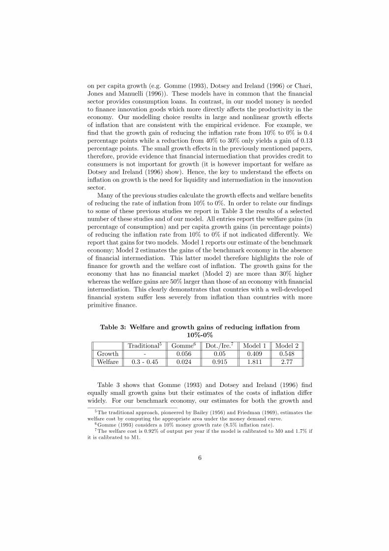
of reducing the rate of inflation from 10% to 0%. In order to relate our findingsto some of these previous studies we report in Table 3 the results of a selectednumber of these studies and of our model. All entries report the welfare gains (inpercentage of consumption) and per capita growth gains (in percentage points)of reducing the inflation rate from 10% to 0% if not indicated differently. Wereport that gains for two models. Model 1 reports our estimate of the benchmarkeconomy; Model 2 estimates the gains of the benchmark economy in the absenceof financial intermediation. This latter model therefore highlights the role offinance for growth and the welfare cost of inflation. The growth gains for theeconomy that has no financial market (Model 2) are more than 30% higherwhereas the welfare gains are 50% larger than those of an economy with financialintermediation. This clearly demonstrates that countries with a well-developedfinancial system suffer less severely from inflation than countries with moreprimitive finance.

Table 3: Welfare and growth gains of reducing inflation from10%-0%

Traditional5 Gomme6 Dot./Ire.7 Model 1 Model 2Growth - 0.056 0.05 0.409 0.548Welfare 0.3 - 0.45 0.024 0.915 1.811 2.77

Table 3 shows that Gomme (1993) and Dotsey and Ireland (1996) findequally small growth gains but their estimates of the costs of inflation differwidely. For our benchmark economy, our estimates for both the growth and

5The traditional approach, pioneered by Bailey (1956) and Friedman (1969), estimates thewelfare cost by computing the appropriate area under the money demand curve.

6Gomme (1993) considers a 10% money growth rate (8.5% inflation rate).7The welfare cost is 0.92% of output per year if the model is calibrated to M0 and 1.7% if

it is calibrated to M1.

6

welfare gains are much higher. We get higher estimates because in our modelmoney and finance facilitates trade of innovation goods that directly affect pro-ductivity in the goods sector. The welfare gains are also larger than thosepresented by Fisher (1981) and Lucas (1981).8 They are higher since the tra-ditional approach does not capture the cost of inflation that origins in a lowerreal growth rate.The proofs of all lemmas and propositions in this paper appear in the Ap-

pendix, unless specified otherwise.

2 The modelConsider a discrete-time economy with many households. The number of house-holds in each type is large and normalized to one. All households have the samediscount factor β ∈ (0, 1). Denote R ≡ (1− β) /β. The households of eachtype are specialized in producing a good which they do not consume; instead,they consume a set of goods produced by other types of households. Goods areperishable between periods. We pick an arbitrary household as the representa-tive household and use lower-case letters to denote its decisions. The decisionsof other households and the aggregate variables are denoted with capital-caseletters. The representative household takes all capital-case variables as given.The utility function in each period is u (qb, s, n), where s is the measure

of shoppers, qb indicates consumption goods per shopper, so that sqb is con-sumption, and n is leisure. For the model to generate balanced growth, we letu(qb, s, n) = ln(sqb)+ln(n

θsϑ).9 The representative household consists of a largenumber of members, who share consumption and regard the household’s utilityas the common objective.10 The measure of members in a household is normal-ized to one. The household divides the members into five groups: a fractionl of members are innovators; a fraction k work in the intermediation/financialsector; a fraction h produce consumption-goods; a fraction n enjoy leisure anda fraction s are buyers in the consumption-goods market. This allocation ofmembers to the five activities (or time) is one of the links between inflation andeconomic growth which we want to focus on in this paper.We define the production function of consumption goods as q (h) where the

input h is the fraction of agents who are producers in the consumption-goodsmarket. We assume that the function q (h) is linear so that q (h) = ah0h, where

8Fisher (1981) and Lucas (1981) estimate the cost of inflation by calculating the appropriatewelfare cost under the money demand curve. Fisher (1981) estimates the cost of increasing therate of inflation from 0% to 10% to be 0.3% and Lucas (1981) to be 0.45%. For a discussionof this estimation procedures and more recent estimates (e.g. Lucas 2000) see Craig andRocheteau (2005).

9 Shouyong: The shopping time does not do anything to this version of the model and sowe could take it out. But if we include it we need that s provides some utility to avoid thatthe household chooses s = 0 (one agent does all the shopping).10The device of a household is used here to maintain tractability, as it enables us to smooth

the matching risk within a household and hence to obtain a degenerate distribution of moneyholdings across households. See Shi (1997).

7

a is the level of productivity of the household’s technology to be described laterand h0 is a constant, with h0 > 0.11

Innovators produce innovation goods which are not useful for their ownhousehold but may be useful for other households. Hence, innovation goodsare traded in a frictional market where innovators meet at random in bilateralmeetings. When two innovators meet, the first agent desires the innovationgood produced by the second agent with probability σ; with the same probabil-ity, the second agent desires the innovation good produced by the first agent.No double-coincidence meeting occurs. In a single coincidence meeting, thebuyer makes a take-it-or-leave-it offer to the seller which consists of an amountof money to be paid by the buyer and a quantity y of the innovation good to beproduced by the seller. Producing y represents a disutility equal to c (y) to theseller, with c (0) = 0, c0 > 0, c00 > 0 and c0 (0) = 0. We will assume the followingfunctional form: c (y) = c0y

α with α > 1 and c0 > 0.Finally, two additional features of the innovation market are important.

First, agents are anonymous and no form of record-keeping is feasible in theinnovations market. Therefore, a medium of exchange is needed for transac-tions to take place. This medium is fiat money, a perfectly storable objectwhich is intrinsically worthless. The need for liquidity to improve the house-holds’ technology is the second link between inflation and economic growth thatwe intend to address. Second, in order to generate a role for financial interme-diation we assume - as in Rocheteau and Wright (2005) or in Berentsen, Mentioand Wright (2008) - that innovators get into the innovation market only prob-abelistically: only one half of the innovators can enter the innovation market.This assumption generates different liquidity needs among innovators. Thosewho cannot enter have "idle" money which they would like to lend earn interestand those who can enter demand more liquidity and are willing to pay for it aswe show below in more detail.If a is the current productivity of the household’s technology in producing

goods, then the productivity of the technology in the next period is:

a+1 = a+ aσ (l/2) y.

The subscripts“+1” indicate the next period throughout the paper. One inter-pretation of a is that it is the stock of human capital, as in Lucas (1988). Likemany endogenous growth models, our model generates long-run growth fromthe non-diminishing marginal productivity of a in the innovation process. Wespecify the innovation sector to deliver long-run growth, rather than using theso-called AK model, because we want to emphasize the allocation of time be-tween different sectors. The modeling is also convenient for finding identificationrestrictions in the calibration, as illustrated later.We assume that in the market for consumption goods a form of record-

keeping is available, so that buyers get credit. Hence, they do not need a mediumof exchange to carry out transactions, but they may buy goods provided that the

11Shouyong: Wecould also model a concave production function q (h) = ah0hη . However,this would require an additional target.

8

household repays them at the end of the period. The purpose of this assumptionis to focus on the role of liquidity in the innovation market, which is supposed toaffect growth, instead of studying how liquidity affects the consumption- goodsmarket. Moreover, we assume that the participants of the goods market takeprices as given. This particular pricing mechanism streamlines the character-ization of the equilibrium and simplifies the algebra; however, we could usealternative pricing mechanisms, such as a form of bilateral bargaining as we dofor trades among innovators.

2.1 The social planner’s allocation

To provide a benchmark against which to measure the efficiency of the equilib-rium, let us first consider the allocation of a social planner. Assume that thesocial planner can dictate all quantities and the allocation of time subject tofeasibility constraints. In this case, there is no need for a credit market, and sok = 0. Denote the planner’s allocation as P = qb, q, y, l, n, h, s, where qb isthe quantity of goods given to a buyer, q is the quantity of goods produced bya household, y is the amount of innovations produced in each bilateral singlecoincidence meeting and l, n, h and s correspond to the allocation of time ineach period. Denote the maximized social welfare function as W (a). Then, theplanner’s allocation solves:

W (a) = maxP

u (qb, s, n)− σ (l/2) c (y) + βW (a+1)

subject to the following constraints:

sqb 6 q (1)

q 6 ah0h (2)

l + n+ s+ h 6 1 (3)

a+1 = a+ aσ (l/2) y (4)

The first term in the welfare function is a household’s total utility from con-sumption and leisure and the second term is the disutility from the productionof innovation goods by (l/2) members who produce with probability σ. Theconstraints (1) and (2) state that the total amount of goods consumed must beequal to the total amount produced, which is determined by the fraction h ofagents and the level of productivity a. The constraint (3) states that the sumof members allocated to the different activities must be equal to 1. Equation(4) is the law of motion of productivity.Denote the solution to the above problem by adding the superscript P to the

variables. The following proposition describes the socially optimal allocation:

Proposition 1 A unique social optimum exists, which is the solution to the

9

following equations:

πp = (α− 1) c (yp) (σ/2) (5)

πp = θ/np = 1/hp = ϑ/sp (6)

1/R = c0 (yp) [1 + (σ/2) lpyp] (7)

1 = lP + nP + sP + hP (8)

The socially efficient rate of growth is:

gp = 1 + σ (lp/2) yP (9)

The quantity yP is increasing in β, θ and ϑ and decreasing in σ. Moreover, wecan verify dlP /dβ > 0, dnP/dβ < 0, dhP /dβ < 0, dsP /dβ < 0 and dqP/dβ < 0.Therefore, the optimal growth rate is increasing in β.The equation (5) comes from the first-order condition on l whereas (6) comes

from the first-order conditions for n, h and s, respectively. (7) results from com-bining the envelope condition on a and the first-order condition on y. Finally,(8) is the constraint (2) which binds in the planner’s solution.

2.2 Financial intermediation

Now we return to the market economy and describe financial intermediation. Be-cause the household allocates money to the innovators before they learn whetherthey have they can enter the innovation market, innovators have different liquid-ity needs after the entry selection is revealed. This generates a role for financialintermediaries that reallocate liquidity from those innovators that have no accessto the innovation market to those that have access. The intermediation/financialsector is perfectly competitive in the sense that there is free entry of banks.Financial intermediaries have no ability to keep records on transactions in

the innovation market. This assumption prevents banks from issuing creditthat supersedes money or directly intermediating the trade in the innovationmarket. However, banks are able to keep financial records on monetary loansand repayments, at a cost. So, borrowing and lending are in terms of money.If a buyer fails to repay a loan, the bank can confiscate money holdings of thebuyer’s household, which ensures that loans are always repaid. Banks take thedeposit rate as given and compete in the loan market. Depositors have perfectinformation about the banks’ financial state and trading histories, which inducesthe banks to always repay the depositors.12

We assume that the production function in the financial sector is such thatlabor input required to produce loans is proportional to the number of loans.13

That is,l/2 = φK. (10)

12Our assumptions of perfect monitoring by the banks on the borrowers and by the deposi-tors on the banks simplify the analysis and enable us to focus on growth. For a relaxation ofthis assumption, see Berentsen, Camera and Waller (2007).13There are several possible alternative specifications. For example, we could also assume

that the labor needed is proportional to the real stock of loans; i.e., B /p = aφK.

10

where l/2 is the number of loans, φmeasures the productivity of the financialsystem and K is the aggregate measure of agents per household working in thefinancial sector. We refer to the case φ→∞ as a perfect loan market, i.e. onein which financial intermediation requires no resources.We indicate the economy-wide average of the amount of borrowing and lend-

ing per household as B and Bd, respectively. The wage bill paid to the financialworkers is the cost of operating the loans in nominal terms. Let w denote thenominal wage rate in the economy. Then, the total nominal cost of loans is wK.A financial intermediary covers the cost of loans with a spread between the loanrate, r , and the deposit rate, rd. Therefore, banks’ profits are

r B − rdBd − wK,

where r B is the interest paid by borrowers to banks, rdBd is the interestpaid by banks to depositors and wK is the wage bill paid to workers in thefinancial sector. In a competitive equilibrium with free entry of banks, banks’profits are zero, so that

r B − rdBd = wK. (11)

Financial intermediaries take the loan rate and the deposit rate as given.There is no strategic interaction among financial intermediaries or between fi-nancial intermediaries and agents. In particular, there is no bargaining overterms of the loan contract.For clarity, let us describe the sequence of events in a period as follows. At

the beginning of the period, each household chooses (l, k, n, s, h), and dividesits holdings of money among the innovators. Then, shoppers and innovatorsleave the household. Each innovator learns if he can enter the market for in-novation goods and decides whether to borrow from or lend to intermediaries.Then, bilateral meetings occur among innovators. Simultaneously, shoppersbuy consumption goods in the final goods market. Once trades are completed,all members return home and give their holdings of money, innovation goodsand consumption goods to the household. Before the period ends, all debts aresettled and households receive a lump-sum monetary transfer from the govern-ment.

2.3 The representative household’s decisions

At the beginning of the period, the household chooses the division of the mem-bers into workers in the financial sector, k, innovators, l, producers h, memberswho enjoy leisure, n, and buyers who enjoy leisure as well s. It allocates moneyamong innovators by giving m/l units of money to each of them. The house-hold decides the quantity of consumption goods per buyer qb and determinesthe offer made by innovators who buy in the innovation market, which consistsof a quantity y of the innovation good and an amount d of money to be givenin exchange. After leaving the household, innovators face equal probability ofentering and not entering the market for innovation goods. This friction createsa role for the financial system, since innovators who enter the market may have

11

incentives to borrow money whereas innovators who cannot enter want to de-posit their money holdings. We indicate by b and bd the amounts borrowed anddeposited by an innovator, respectively. At the end of the period, the householdchooses future holdings of money, m+1, and the future productivity, a+1. Thedecision variables of the household are then:

z ≡ [qb, l, n, k, h, s, d, y, b , bd,m+1, a+1] .

Let m denote a representative household’s holdings of money at the begin-ning of a period. The household’s value function is V (a,m). Define:

ω ≡ β∂V (a+1,m+1)

∂m+1and λ ≡ β

∂V (a+1,m+1)

∂a+1.

The variable ω is the shadow value of money next period and λ the shadowvalue of future productivity, both of which are discounted to the current period.The representative household’s problem is to choose z to solve the following

problem:

V (a,m) = maxz

u (qb, s, n)− σ (l/2) c (Y ) + βV (a+1,m+1)


1 ≥ l + k + s+ h+ n (π) (12)

d ≤ m/l + b [σ (l/2)μ] (13)

bd ≤ m/l [(l/2)ψ] (14)

dΩ ≥ c (y) [σ (l/2) ς] (15)

a+1 = a+ σ (l/2) ya (16)

m+1 −m = p (h0ah− sqb) + σ (l/2) (−d+D) (17)

+(l/2) (bdrd − b r ) + wk + T

where T is a lump-sum transfer or tax and p is the nominal price of con-sumption goods. The first term in the objective function represents the utility ofconsuming the goods brought by buyers to the household and enjoying leisure.The second term is the disutility from producing innovation goods and the thirdterm is the discounted future value. Notice that the amount of production byan innovator is not subject to the decision of the household since it is proposedby buyers in each meeting (we denote the amount produced with a capital letterY ).The constraint (12) is the time constraint of the household. The constraint

(13) specifies that an innovator who buys from another innovator cannot spendmore money than the sum of his money holdings, m/l, and the money borrowed,b . According to (14), the amount of deposits of an agent is bounded by hismoney holdings. (15) is the seller’s participation constraint: for a seller to bewilling to produce y, the value of the money received, dΩ, must be at least ashigh as the disutility c (y). The constraint (16) is the law of motion of produc-tivity described earlier. The law of motion of the household’s holding of money

12

is (17). The term p (sqb − ph0ah) is the net income from trading in the finalgoods market. The term σ (l/2) (−d+D) is the net income from trading in theinnovation goods market since (σ/2) innovators spend an amount d to buy inno-vation goods (σ/2) of them receive an amount D when selling innovation goods.The term (l/2) (bdrd − b r ) is the net income from borrowing and lending sincean equal number of innovators borrow money and deposit money. Finally, thehousehold receives wage payments for workers in the financial sector, wk, andlump-sum monetary transfers from the government, T .In the bilateral bargaining in the market for innovation goods we assume

that the buyer has all the bargaining power. Therefore, the buyer solves:

maxd,y

(aλy − dω)

s.t. dΩ ≥ c (y) , d ≤ m/l + b

The pay-off to the buyer is the gain from acquiring a quantity y of goods toimprove the household’s productivity, measured by aλy, minus the value of themoney paid to the seller, dω. When solving this problem, the buyer must satisfythe seller’s participation constraint and the cash constraint.

2.4 Equilibrium definition and optimal conditions

We focus on the monetary equilibrium which is symmetric in the sense that thedecisions are the same for all households. Throughout this paper, monetarypolicy is such that monetary transfer maintains the gross rate of money growthat a constant level γ ≥ β.With the above focus, a monetary equilibrium consists of the representa-

tive household’s decisions, z, other household’s decisions, Z, and interest rates,rd ≥ 0 and r ≥ 0, which meet the following requirements: (i) z solves the rep-resentative household’s maximization problem above; (ii) the decisions are sym-metric across households: z = Z; (iii) the credit market and the consumption-good markets clear; and iv) the seller’s participation constraint in the innovationmarket is non-negative.We state the market clearing condition for consumption goods as:

h0ah = sqb (18)

The first-order condition on qb is:

1

qb= ωps (19)

That is, the higher utility from increasing qb and, hence, consumption, shouldbe offset by the value of money used to settle the purchase.Denote σ (l/2)μ and (l/2)ψ the multipliers associated to (13) and (14),

respectively. The first-order conditions on bd and b are as follows:

ψ = rdω (20)

σμ = r ω (21)

13

The shadow prices associated to the deposit constraint and the cash constraintare given by the deposit and borrowing interest rates, respectively. We indicateby σ (l/2) ς the multiplier associated to (15). The first-order condition on d andy are the following:

ω (ς − 1)− μ = 0

aλ− c0 (y) ς = 0

Using (21), we rewrite them as follows:

ς =r

σ+ 1 (22)

aλ = c0 (y)³rσ+ 1´

(23)

Next, we calculate the optimal conditions regarding the allocation of time.We call π the multiplier associated to (12). The first-order condition on l is:

−σ (1/2) c (Y )− π − (1/2) (σμ+ ψ) (m/l) + λa (σ/2) y

+σ (1/2) (−d+D) + (1/2)ω (bdrd − b r ) = 0

This condition says that the marginal cost of allocating an additional mem-ber of the household to the innovation market is given by a higher cost ofproducing innovation goods, the opportunity cost of not allocating an extramember to the rest of the activities and a decrease in the amount of moneyallocated to each innovator. It also says that the marginal benefit of an addi-tional innovator comes from a higher productivity in the future. In addition,allocating an extra member to the innovation sector affects the money holdingsof the household at the end of the period, as it is described by the other terms:it increases the money spent and received in the market for innovation goodsand entails higher interest for the household’s deposits as well as higher interestpayments.In a symmetric equilibrium, y = Y and d = D. These equalities allow us to

write the first-order condition on l as follows:

−σ (1/2) c (y)−π−(1/2) (σμ+ ψ) (m/l)+λa (σ/2) y+(1/2)ω (bdrd − b r ) = 0(24)

The first-order condition on n is:

π = θ/n (25)

Similarly, the first-order condition on s is:

1 + ϑ

s− π − ωpqb = 0

According to (25), the opportunity cost of a member enjoying leisure should beequal to the marginal utility that he provides to the household. In the conditionfor s the utility from a greater quantity of goods for consumption and the value

14

of money to buy them are considered as well. This condition may be simplifiedas follows, using (19):

π = ϑ/s

The optimal condition for k is:

π = ωw (26)

The first-order condition on h is:

π = ωph0a

Using (19) and (18), it reduces to:

π = 1/h

Finally, we calculate the envelope conditions for a and m. The envelopecondition for a is

λ−1/β = λ [1 + σ (l/2) y] + ωph0h (27)

The envelope condition for m is:

ω−1/β = ω + (1/2) (σμ+ ψ) (28)

Envelope conditions state that the current value of an asset (m or a) is equalto the future value of the asset plus the additional value of the asset in the cur-rent exchange. According to (27), a marginal unit of productivity results in[1 + σ (l/2) y] units of future productivity, the value of which is λ [1 + σ (l/2) y].In addition, a marginal unit of productivity saves production cost in the ex-change, as it is computed in the second term of the condition for a. Similarly, in(28), μ is the shadow value of money that reflects how the household’s constrainton money is alleviated when an additional unit of money is acquired.

3 Balanced GrowthIn this section, we characterize the balanced growth path of the economy. Abalanced growth path is defined as an equilibrium in which productivity, a,grows at a constant gross rate g, and interest rates are non-negative and finiteconstants (i.e., 0 ≤ rd ≤ r <∞). It is clear from (16) that

g = 1 + σ (l/2) y. (29)

Lemma 1 The balanced growth path has the following properties: (i) l, k, h, sand n are constants in (0, 1) with l+ k + h+ n+ s = 1; (ii) qb grows at rate g;(iii) the marginal value of money, ω, decreases at rate γ; and (iv) the marginalvalue of productivity, λ, falls at rate g. Interest rates, rd and r , satisfy:

(γ − β) /β = (r + rd) /2 (30)

(r − rd)φ = (α− 1) (σ + r ) (31)

15

The equilibrium solution for π, y, l, n, s, k, h is determined by:

π = (α− 1) c (y) (σ/2 + r /2) (32)

π = θ/n = 1/h = ϑ/s (33)

1/R = c0 (y) [1 + σ (l/2) y] (1 + r /σ) (34)

1 = l + n+ s+ h+ k (35)

l/2 = φk (36)

The value of money and consumption satisfy ωm = (l/2) c (y) and sqb = h0ah.Moreover, drd/dγ > 0, dr /dγ > 0 and dy/dγ < 0.

Equation (30) comes from (28), which is the envelope condition of moneyholdings. The condition (31) comes from the zero-profit condition of intermedia-tion. Equation (32) comes from the first-order condition for l whereas equationsin (33) come from the first-order conditions for n, h and s, respectively. Theequation in (34) is the envelope condition for a which comes from (27). Finally,(35) is the time constraint of the household and (36) replicates the productionfunction of the financial sector.The reminder of this section needs more work....Denote gC and gN the real growth rates that prevail in an economy with

credit market and in an economy without credit market, respectively. Similarly,let yC and yN be the respective quantities of y traded in these economies.

Lemma 2 When γ > β and there is no credit market, the equilibrium allocationπ, y, l, n, s, h satisfies the following equations:

π = (α− 1) c (y) [σ/2 + (γ − β) /β] (37)

π = θ/n = 1/h = ϑ/s (38)

1/R = c0 (y) [1 + σ (l/2) y] [1 + 2 (γ − β) / (βσ)] (39)

1 = l + s+ h+ n (40)

Moreover, c0¡yC¢gC > c0

¡yN¢gN for γ > β.

To examine how monetary policy affects long-run growth, let us first analyzean economy with a perfect loan market (i.e., with φ→∞) and then an economywith an imperfect loan market (i.e., with φ < ∞). Taking the limit φ → ∞ inLemma 1, it is straightforward to prove the following proposition on an economywith a perfect loan market:

Proposition 2 For γ > β and φ → ∞, the equilibrium allocation (rd, r ,-π, y, l, n, s, k, h) satisfies rd = r = r = (γ − β) /β and k = 0. Moreover,π, y, l, n, s, h satisfy

π = (α− 1) c (y) [σ/2 + (γ − β) / (2β)] (41)

π = θ/n = 1/h = ϑ/s (42)

1/R = c0 (y) [1 + (σ/2) ly] [1 + (γ − β) /(βσ)] (43)

1 = l + s+ h+ n (44)

16

The balanced growth path depends on money growth as follows: dr/dγ > 0dy/dγ < 0.

Corollary 1 For any γ > β, the quantity of innovation goods traded in an econ-omy with a perfect credit market is strictly larger than in an economy withoutcredit market.

4 Quantitative AnalysisIn this section we calibrate the model to quantify the welfare and growth effectsof inflation and an improvement in the productivity of financial intermediation.

4.1 Calibration

We choose the following functional forms:

u(qb, n, s) = ln (sqb) + ln¡sϑnθ

¢, c(y) = c0y

α,

With the above functional forms, the parameters to be identified are asfollows: (i) preference parameters: (β, θ, ϑ, h0, c0, α); (ii) technology parameters:(φ, σ); (iii) policy parameters: the money growth rate γ. To identify theseparameters, we calibrate the model to US data. Table 4 lists the identificationrestrictions and the identified values of the parameters.

Table 4: Calibration and parameter values

parameters values identification restrictionsβ 0.9824 deposit rate = 0.075γ 0.0826 inflation rate = 0.057σ 0.0225 bank credit= 0.44h0 1 normalization to 1α 27.628 working time/total time = 0.2c0 3.454 ∗ 10−18 shopping time/working time= 0.1116φ 112.225 loan officers/employment = 0.0025ϑ 0.256 per capita growth rate = 0.024θ 8.911 R&D expenditure to GDP ratio= 0.02

The identification restrictions come from two sources. First, the inflationrate, bank credit and per capita growth rate matches the ones of the averagelow inflation country (see Table 2).14 Second, all other restrictions are fromUS data: the deposit rate matches the average interest rate on the US 3-monthdeposit certificates from 1965 -1995;15 as in King and Rebelo (1993), we choosethe balanced-growth fraction of time working to be 20%; according to a report

14We use the measure of the size of the financial sector, priv, from Levine, Loayza and Beck(2000). The measure priv contains all claims on the private sector of banks that take depositsdivided by GDP. From Table 2, the average priv among low-inflation countries is priv = 0.44.15A certificate of deposit is a time deposit. It is insured and thus virtually risk-free.

17

on occupational employment and wages by the Bureau of Labor Statistics (BLS,2006), in May 2005 the fraction of loan officers to total employment was 0.0025;16

from the time-use diary reported in Juster and Stafford (1991), the ratio ofshopping time to working time is 11.16%; from the OECD data reported inGrossman and Helpman (1995, p10), the average ratio of R&D expenditure toGDP is about 2% in the US.In the Appendix we detail the calibration procedure which uses these re-

strictions to compute the parameter values listed in Table 4.

Table 5: Calibration

Inflation Growth SizeData Model Data Model Data Model

Low 0.057 0.057 0.024 0.024 0.44 0.441Mid 0.092 0.092 0.019 0.023 0.271 0.359High 0.316 0.316 0.013 0.018 0.18 0.154

Table 5 compares the model’s predictions on inflation, the growth rate andthe size of the financial sector with the data. We have calibrated the model tothe average low-inflation country which explains why the model and the dataare the same in the row labelled "Low".Our model predicts an non-linear relationship between the financial sector

measure bank credit and inflation as Figure 1 shows. At low levels of inflationan increase in inflation reduces the size of the financial sector more than at highlevel of inflation.16According to this report, in May 2005, 332690 people were working as loan officers and

the total employment was 130307850. The ratio 0.0025 is similar to the 0.0028 reported inDotsey and Ireland (1996)

18

Figure 1: Bank credit and inflation

0 20 40 60 80Average inflation

20

40

60

80

100

120knaB

tiderc(%

foPDG)

High Inflation

Med Inflation

Low Inflation

Model simulation

A highly interesting aspect of the model, consistent with the data, is the non-linear relationship between inflation and real growth. At high rates of inflation,10% reduction in inflation has almost no growth effects while at low rates ofinflation a 10% reduction of inflation has large growth effects. We will discussthis property of the model in subsection 4.5.

4.2 Welfare analysis

With the identified model, we now quantify the cost of inflation, Π, and thebenefit of an exogenous improvement in financial productivity, φ. We focus onthe balanced growth path.Following the literature (e.g. Lucas, 2000 or Lagos and Wright, 2005), we

measure the welfare cost of inflation at Π relative to Π0 by asking how muchconsumption in percentage agents would be willing to give up in order to changeinflation from Π to Π0. Similarly, we measure the welfare benefit of an improve-ment in financial productivity from φ to φ0 by asking how much consumptionin percentage agents would be willing to give up for the improvement. To ex-press these measures formally, let Π be any given inflation rate, φ any level ofthe exogenous component of financial productivity, and (1 −∆) any rate of aconsumption tax. Slightly abusing an earlier notation, we write the household’sexpected discounted utility under (Π,∆, φ) as:

W (Π,∆, φ) =∞Xt=1

βt−1£ln (∆sqb,t) + ln

¡nθsϑ

¢− σ (l/2) c (y)

¤where all the quantities (y, qb, l, n, s) take their equilibrium values when ∆ = 1.

19

Note that qb is indexed by t because it evolves over time according to the growthrate g. This expression can be rewritten as follows:

W (Π,∆, φ) =1

1− β

∙ln¡nθsϑ

¢+ ln (∆sqb,1)− σ (l/2) c (y) +

β

1− βln (g)

¸For any fixed φ, the welfare cost of inflation at Π relative to Π0 is the value of∆ that solves W (Π0,∆, φ) =W (Π, 1, φ). Similarly, for any fixed Π, the welfarebenefit of improving the exogenous component of financial productivity from φto φ0 is the value of ∆ that solves W (Π,∆, φ0) =W (Π, 1, φ).

4.3 The growth and welfare effects of inflation

Table 6 characterizes the balanced-growth equilibrium calibrated to the averagelow-inflation country. It compares this equilibrium to those obtained with zeroinflation, the average inflation rate of the medium-inflation countries (9.21%),and the average inflation rate of the high-inflation countries (31.6%).17 It alsoreports for each country type, the welfare and per capita growth gains frommoving to a zero inflation rate policy.

Table 6: Effects of inflation

0% 5.71% 9.21% 31.6%Time innovating 0.1228 0.1122 0.1072 0.0872Time working in finance 0.0005 0.0005 0.0005 0.0004Shoppingtime 0.0221 0.0223 0.0224 0.023Leisure 0.7684 0.7777 0.7821 0.7997Time producing 0.0862 0.0873 0.0878 0.0898

Interestrate wedge 0.0374 0.0545 0.0654 0.1403Bank credit HprivL 0.676 0.4408 0.3589 0.154Participationrate 0.0614 0.0561 0.0536 0.0436

Innovation goods HyL 4.7999 4.7396 4.7115 4.6021GDP 1.0379 1.0261 1.0219 1.0113

Growth rate 0.0268 0.0241 0.0229 0.0182Growth loss Hpercentage pointsL 0. 0.2627 0.3848 0.8598

Welfare loss H%of consumptionL 0. 1.0528 1.6221 4.024

An increase in inflation changes total labor supply and its composition. Ta-ble 6 shows that as the inflation rate rises, the household reduces the time spentin the innovation sector. It also slightly reduces the time working in finance. In

17The welfare and growth gains reported for the medium inflation country correspondsroughly to gains obtained from the standard exercise of reducing the rate of inflation from 10percent to zero percent.

20

contrast, the household increases leisure, shopping time and the time producingconsumption goods. Thus, any additional labor allocated to either leisure, pro-duction or shopping as a result of higher inflation comes mainly from reducinglabor in the innovation sector. The substitution of labor out of innovation andinto leisure, shopping and production reduces the per capita growth rate.The effects of inflation on growth are large. For the average medium-inflation

country, reducing its inflation from the average (9.2%) to zero increases thelong-run growth rate by 0.385 percentage points. For the average high-inflationcountry, reducing its average inflation to zero increases the long-run growth rateby 0.86 percentage points. These large effects of inflation on per capita growthfall into the range of empirical estimates obtained from cross-country studies(see the references in the Introduction). They distinguish the quantitative per-formance of our model from those of previous models such as Gomme (1993) orDotsey and Ireland (1996), who find that reducing inflation to zero in a similarexperiment increases growth by only 0.05 percentage points.Higher rates of inflation also affect the financial market. Table 6 shows that

the interest rate wedge increases with inflation. At 9.2 percent inflation thewedge is 6.5%. The wedge becomes 14% for the average high inflation country.Participation in the financial market, measured by the fraction of innovators whotake out loans, and the ratio of loans to GDP strongly decrease with inflationshowing a reduction of the financial market size. Finally, aggregate output andthe amount of innovation goods traded decrease as inflation increases.

4.4 Decomposing the welfare and growth effects: alloca-tion of time

Table 6 shows that the welfare cost of inflation are 1.053% of consumptionfor the average low-inflation country, 1.622% for the average medium inflationcountry and 4.024% for the average high-inflation country. Moreover, inflationhas large negative effects on growth. In this subsection, we investigate howthe distortions of inflation on various margins of labor supply contribute to thewelfare and growth effects of inflation.

21

Table 7: Constant labor in the innovation sector






First, let us examine whether the choice of labor in innovation is importantfor the effects of inflation. To do so, Table 7 considers a version of the modelwith exogenous time devoted to innovation. This version of the model keepsthe fraction of agents working in innovation constant at its calibrated valuel∗ = 0.1122.18 In contrast to Table 6, the allocation of time in Table 7 isinelastic. The quantity of innovation goods traded in the innovation sector y isonly slightly smaller in Table 7 than in Table 6. As a result, the growth lossesof inflation are substantially smaller when l is constant. Moreover, the realoutput and the measure priv turn out to be less sensitive to inflation. Anothercontrast of Table 7 with Table 6 is that the welfare cost of inflation is smaller.For example, 9.21% inflation costs 1.379% of consumption under constant l,rather than 1.622% as under endogenous l. This clearly indicates that the effectof inflation on the choice for l matters for generating the welfare cost estimatesreported in Table 6.

18Tables 6-10 are constructed as follows. First, we replace one equilibrium condition bysetting x = x∗ where x is the variable under consideration and x∗ its calibrated value. Second,we simulate the model for different values of inflation. For example, for table 6, x = l andx∗ = l∗.Note that we do not recalibrate the model since this not necessary. A recalibration of the

model for each experiment - using the same targets - would yield the same values for thecalibrated parameters as in the baseline case. The reason is that x is held constant at itsequilibrium value obtained from the baseline calibration.

22

Table 8: Constant leisure






Second, let us analyze whether the leisure choice is important for the effectsof inflation. To do so, Table 8 considers a version of the model where theamount of leisure is fixed at the calibrated level n∗ = 0.777. It is clear fromTable 8 that the allocation of time is again rather inelastic, because a largepart of it (i.e., leisure) is fixed. A comparison with Table 6 makes it moreevident that the increase in leisure in the general model is at the expense ofinnovation rather than reducing the time producing, shopping or trading, sincethe resources assigned to these three activities are similar in Tables 6 and 8.This explains the large differences in the growth effects between the completemodel and the version with n constant: in the former case, growth losses aremore than 4 times higher for the three groups of countries. In addition, fromTable 8 it is noticeable that endogenizing the choice of leisure is importantfor determining the welfare cost of inflation, since this is smaller for n fixed.Actually, its estimate is very close to the one for l fixed, which is consistent withthe fact that, when inflation changes, households adjust their choices basicallythrough leisure and innovation.

23

Table 9: Constant shopping time



Innovationgoods HyL 4.7999 4.7396 4.7115 4.602GDP 1.0378 1.0261 1.022 1.0114



Table 9 shows the simulation results with constant shopping time s∗ =0.0223. If we compare the results with the benchmark model (Table 6) onecan see that the differences are small. The reason is that the s is not very sen-sitive to changes in inflation. Moreover, its calibrated value is low.19 Finally,we have also studied a version of the model where the time for production ofconsumption goods h is held constant. We obtain similar results as shown inTable 9 and we therefore omit to present them.

4.5 Why is there a non-linear relation between inflationand growth?

As we mentioned before the effects of inflation on per capita growth are highlynonlinear. At high rates of inflation, 10% reduction in inflation has almost nogrowth effects while at low rates of inflation a 10% reduction of inflation haslarge growth effects (see Figure 1 below). In this section we show that the non-linearity is driven by the choice of y which is affected by inflation and not bythe allocation of time. Inflation decreases the value of money and hence thewillingness of a seller to produce goods in a bilateral meeting. Therefore, thequantity y traded per buyer in the innovation sector decreases with inflation.In order to estimate the importance of this channel, Table 10 presents a versionof the model in which y is taken as exogenous. It is kept at its calibrated valuey∗ = 4.7396 for all inflation rates considered.

19This result is different from the findings by Love and Wen (1999), who attribute importantwelfare effects of inflation to the time-costs of transacting featured by their model.

24

Table x: constant y

0% 5.71% 9.21% 31.6%Time innovating 0.1202 0.1122 0.1074 0.0781Time working in finance 0.0005 0.0005 0.0005 0.0003Time trading 0.0221 0.0223 0.0224 0.0232Leisure 0.7706 0.7777 0.7819 0.8077Time producing 0.0865 0.0873 0.0878 0.0906

Interestrate wedge 0.0528 0.0545 0.0555 0.0615Priv 0.4714 0.4408 0.4223 0.3092Participationrate 0.0601 0.0561 0.0537 0.0391

y 4.7396 4.7396 4.7396 4.7396GDP 1.028 1.0261 1.0249 1.018

Growthrate 0.0259 0.0241 0.0231 0.0167Growth loss (percentage points) 0. 0.1738 0.2783 0.9117

Welfare loss (%of consumption) 0. 0.1145 0.2256 1.5538

Interestingly, the growth loss when y is constant is similar to the estimate ofthe general model for the high-inflation countries, but it is considerably smallerfor the low-inflation and medium-inflation countries. For the low-inflation coun-tries, the loss in the growth rate is equivalent to 0.174 percentage points for yfixed against 0.263 percentage points for y endogenous. These figures are 0.278and 0.385 percentage points, respectively, for the medium inflation countries.This result clearly suggests that the non-linear relationship between inflationand growth predicted by the model is due to changes in y across inflation rates.To illustrate this, we have plotted in Figure 2 the growth gains predicted by themodel that result from a reduction in inflation of 10 percentage points at eachinflation rate. In the same figure, we have plotted the growth gains predictedby the version of the model with y constant. Comparing both curves, it is clearthat the non-linearity of the relation between inflation and per capita growth isentirely driven by the choice of y that changes in inflation.In previous models (Gomme, 1993; Dotsey and Ireland, 1996; and others) the

only mechanism which affected the per capita growth rate was the allocation oftime. These authors found very small growth effects of inflation and, moreover,these effects were linear. If we hold constant y at its calibrated value in ourmodel, so that only the allocation of time affects the growth rate, we still havelarge effects of inflation on growth but they become linear. Thus, our modelnot only predicts large effects of inflation on growth but, in addition, they arehighly non-linear. The reason why we get these non-linear effects is that thecost of producing y is convex and, further, the bargaining solution for y dependson the value of money, which is not linear in the inflation rate.

25

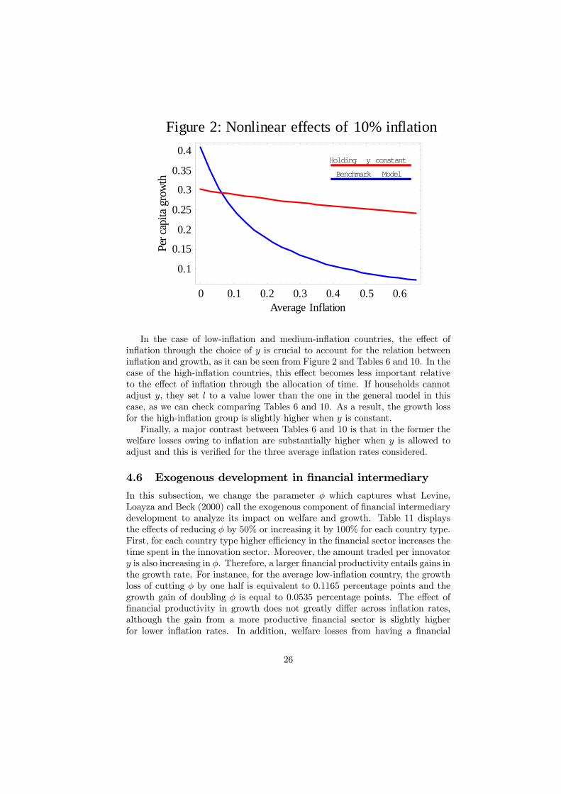
Figure 2: Nonlinear effects of 10% inflation

0 0.1 0.2 0.3 0.4 0.5 0.6Average Inflation

0.1

0.15

0.2

0.25

0.3

0.35

0.4reP

atipachtworg

Benchmark Model

Holding y constant

In the case of low-inflation and medium-inflation countries, the effect ofinflation through the choice of y is crucial to account for the relation betweeninflation and growth, as it can be seen from Figure 2 and Tables 6 and 10. In thecase of the high-inflation countries, this effect becomes less important relativeto the effect of inflation through the allocation of time. If households cannotadjust y, they set l to a value lower than the one in the general model in thiscase, as we can check comparing Tables 6 and 10. As a result, the growth lossfor the high-inflation group is slightly higher when y is constant.Finally, a major contrast between Tables 6 and 10 is that in the former the

welfare losses owing to inflation are substantially higher when y is allowed toadjust and this is verified for the three average inflation rates considered.

4.6 Exogenous development in financial intermediary

In this subsection, we change the parameter φ which captures what Levine,Loayza and Beck (2000) call the exogenous component of financial intermediarydevelopment to analyze its impact on welfare and growth. Table 11 displaysthe effects of reducing φ by 50% or increasing it by 100% for each country type.First, for each country type higher efficiency in the financial sector increases thetime spent in the innovation sector. Moreover, the amount traded per innovatory is also increasing in φ. Therefore, a larger financial productivity entails gains inthe growth rate. For instance, for the average low-inflation country, the growthloss of cutting φ by one half is equivalent to 0.1165 percentage points and thegrowth gain of doubling φ is equal to 0.0535 percentage points. The effect offinancial productivity in growth does not greatly differ across inflation rates,although the gain from a more productive financial sector is slightly higherfor lower inflation rates. In addition, welfare losses from having a financial

26

productivity that is half the calibrated productivity are similar among countrytypes and represent about 1% of consumption.

Table 11: Exogenous increase in productivity

fê2 2f fê2 2f fê2 2fTime innovating 0.1074 0.1144 0.1024 0.1094 0.0822 0.0894Time working in finance 0.001 0.0003 0.0009 0.0002 0.0007 0.0002Shoppingtime 0.0224 0.0223 0.0226 0.0224 0.0231 0.0229Leisure 0.7815 0.776 0.7859 0.7803 0.0007 0.0002Time producing 0.0877 0.0871 0.0882 0.0876 0.0902 0.0895

Interestrate wedge 0.1251 0.0256 0.1502 0.0307 0.3232 0.0658Bank credit HprivL 0.365 0.4798 0.2961 0.3913 0.1252 0.169Participationrate 0.0537 0.0572 0.0512 0.0547 0.0411 0.0447

Innovationgoods HyL 4.7151 4.7506 4.687 4.7226 4.5777 4.6131GDP 1.0278 1.025 1.024 1.0207 1.0138 1.0099

Growth rate 1.0057 1.0061 1.0054 1.0058 1.0042 1.0046Growth loss HppL 0.1165 -0.0535 0.1159 -0.0532 0.1128 -0.0517

Welfare loss H%of cL 1.0632 -0.5115 1.0656 -0.5147 0.9826 -0.4814

Low inflation Medium inflation High inflation

27

AppendixProof of Proposition 1The planner chooses P = qb, q, y, l, n, h, s to maximize the following welfare

function:W (a) = max

Pu (qb, s, n)− σ (l/2) c (y) + βW (a+1) (45)


sqb ≤ q (46)

q ≤ ah0h (47)

1 ≥ l + n+ s+ h (48)

a+1 = a+ aσ (l/2) y (49)

We rewrite (45) using (46), (47) and the functional form of u (qb, s, n):

W (a) = maxPln (ah0h) + ln

¡sϑnθ

¢− σ (l/2) c (y) + βW (a+1)

subject to the constraints:

1 ≥ l + n+ s+ h

a+1 = a+ aσ (l/2) y

The first-order condition on y is:

λa = c0 (y) (50)

The first-order conditions for n, h and s are as follows:

π = θ/n (51)

π = 1/h (52)

π = ϑ/s (53)

The first-order condition on l is:

λay − c (y) = (2/σ)π

Using (50), it becomesπ = (α− 1) c (y) (σ/2) (54)

The envelope condition for a is:

λ−1β

= λ [1 + σ (l/2) y] + 1/a

We rewrite it using (50):

1/R = c0 (y) [1 + σ (l/2) y] (55)

28

Finally, constraint (48) binds in the planner’s choice, so that:

1 = l + n+ s+ h (56)

Equations (51)-(56) form the planner’s solution stated in Proposition 1. Tosee that a unique solution to the above system exists, we rewrite (55). First, wereplace l with (56) and then n, h and s with (51), (52) and (53) as follows:

1/R = c0 (y)

∙1 + (σ/2) y

µ1− θ + ϑ+ 1

π

¶¸Then, we replace π using (54) and rearrange to get:

c0 (y) [1 + (σ/2) y] = 1/R+α (θ + ϑ+ 1)

α− 1 (57)

From (57) we obtain the solution for the optimal value of y. The left-handside in (57) is monotonously increasing in y, is equal to 0 when y = 0 andapproaches +∞ as y approaches +∞. Since the right-hand side is constant,given σ, β, α, ϑ and θ, a unique solution for y exists. The solution for n comesfrom (51) and it is unique since the solution for y is unique. Analogously, thesolutions for h, s and l, which are recursively obtained from (52), (53) and (56),are unique. Finally, it is straightforward to verify that y is increasing in β, θand ϑ and decreasing in σ and that dn/dβ < 0, dh/dβ < 0, ds/dβ < 0 anddl/dβ > 0.Proof of Lemma 1To get a two-equation system in rd and r , we first rewrite the envelope

condition on m (28) using the first-order conditions on bd and b (20) and (21)to get (30). Second, we rewrite the banks’ zero-profit condition (11). Thetotal amount of borrowing is equal to the total amount of deposits, so thatB = Bd. In addition, B is equal to (l/2) b = (l/2) bd, which we can rewrite as(l/2) (m/l). Therefore, (11) becomes:

ω (m/l)φ (r − rd) = π (58)

where we have used the production function of loans (10) and the first-ordercondition on k (26). We set ω (m/l) = ω (d/2) = c (y) /2 to get:

c (y)φ (r − rd) /2 = π (59)

Besides, we rewrite the first-order condition on l (24) using (20), (21) and(23)

(α− 1) (r + σ) (1/2) c (y) = π (60)

Combining (59) and (60) yields the second equation in r and rd (31). (32)and (33) have already been derived whereas (27) is the envelope condition for athat results from using (23). To see that ωm = (l/2) c (y) simply combine (58)

29

with (59). To see that drd/dγ > 0 and dr /dγ > 0 we pin down r and rd from(30) and (31) as follows:

rd = 2 (γ − β) /β − r (61)

r =(α− 1)σ + 2φ (γ − β) /β

2φ− (α− 1) (62)

From (61) and (62), we know that the solution for r and rd is unique. Inaddition, we verify:

dr /dγ =2φ/β

2φ− (α− 1) > 0

drddγ

= 2/βφ− (α− 1)2φ− (α− 1) =

2φ (σ + rd)

β [2φ− (α− 1)] (σ + r )> 0

where we have used (31). To verify that dy/dγ < 0 we use the system inLemma 1 to get an equation in y. First , we get an expression for l from thetime constraint (35), replacing h, n and s with the first-order conditions onthem stated in (33) and k with the production function of loans (36):

l =1− (θ + ϑ+ 1) /π

1 + 1/ (2φ)

Then, we replace l in the envelope condition for a (34). We also use (60) toreplace π and (62) to replace r :

1/R+α (θ + ϑ+ 1)

(α− 1) [1 + 1/ (2φ)] = c0 (y)

µ1 +

(σ/2) y

1 + 1/ (2φ)

¶1 + (γ − β) / (σβ)

1− (α− 1) /2φ

From this equation it is straightforward to compute dy/dγ < 0. It is alsopossible to verify that a unique solution for y exists. As a result, the solution isunique for π, l, n, s and h.Proof of Lemma 2In the absence of credit market, the representative household solves the

following problem:

V (a,m) = maxz

u (qb, s, n)− σ (l/2) c (Y ) + βV (a+1,m+1)


1 ≥ l + s+ h+ n (π)

d ≤ m/l [σ (l/2)μ]

dΩ ≥ c (y) [σ (l/2) ς]

a+1 = a+ σ (l/2) ya

m+1 −m = p (h0ah− sqb) + σ (l/2) (−d+D) + T

30

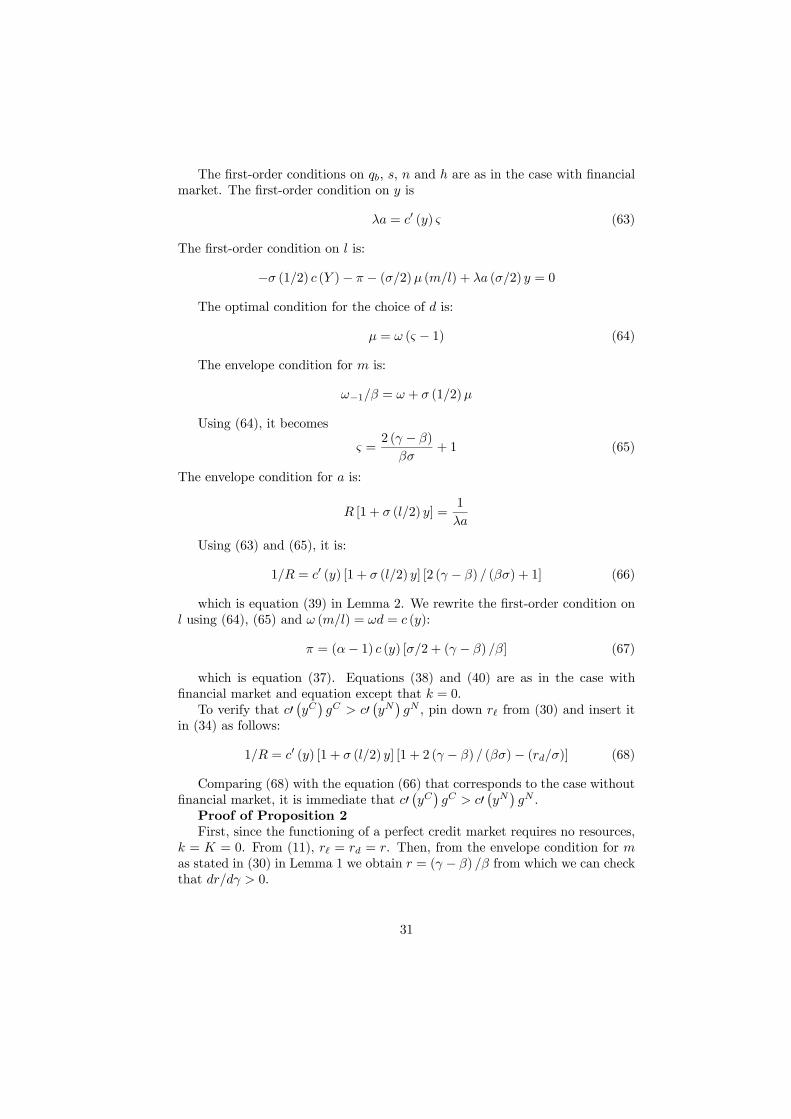
The first-order conditions on qb, s, n and h are as in the case with financialmarket. The first-order condition on y is

λa = c0 (y) ς (63)

The first-order condition on l is:

−σ (1/2) c (Y )− π − (σ/2)μ (m/l) + λa (σ/2) y = 0

The optimal condition for the choice of d is:

μ = ω (ς − 1) (64)

The envelope condition for m is:

ω−1/β = ω + σ (1/2)μ

Using (64), it becomes

ς =2 (γ − β)

βσ+ 1 (65)

The envelope condition for a is:

R [1 + σ (l/2) y] =1

λa

Using (63) and (65), it is:

1/R = c0 (y) [1 + σ (l/2) y] [2 (γ − β) / (βσ) + 1] (66)

which is equation (39) in Lemma 2. We rewrite the first-order condition onl using (64), (65) and ω (m/l) = ωd = c (y):

π = (α− 1) c (y) [σ/2 + (γ − β) /β] (67)

which is equation (37). Equations (38) and (40) are as in the case withfinancial market and equation except that k = 0.To verify that c0

¡yC¢gC > c0

¡yN¢gN , pin down r from (30) and insert it

in (34) as follows:

1/R = c0 (y) [1 + σ (l/2) y] [1 + 2 (γ − β) / (βσ)− (rd/σ)] (68)

Comparing (68) with the equation (66) that corresponds to the case withoutfinancial market, it is immediate that c0

¡yC¢gC > c0

¡yN¢gN .

Proof of Proposition 2First, since the functioning of a perfect credit market requires no resources,

k = K = 0. From (11), r = rd = r. Then, from the envelope condition for mas stated in (30) in Lemma 1 we obtain r = (γ − β) /β from which we can checkthat dr/dγ > 0.

31

(42) and (44) are straightforward. To get (41), we replace r = r = (γ − β) /βin the analogous equation in Lemma 1 (32). To get (43), we also replace r in(34). That dy/dγ < 0 may be shown as in the system in Lemma 1. When thefinancial market is perfect, the equation that solves for y reduces to:

c0 (y) [1 + (σ/2) y] [1 + (γ − β) / (βσ)] = 1/R+α (θ + ϑ+ 1)

α− 1 (69)

Proof of Corollary 1To get to an equation in y in the case with no credit market, we rewrite (66)

replacing l with the time constraint (40) and then n, h and s as we did above,so that we have:

1/R = c0 (y)

∙1 + (σ/2)

µ1− θ + ϑ+ 1

π

¶y

¸[2 (γ − β) / (βσ) + 1]

Then, we replace π with (67):

c0 (y) [1 + (σ/2) y] [1 + 2 (γ − β) / (βσ)] = 1/R+α (θ + ϑ+ 1)

α− 1

Comparing the solution for y from this equation without credit market withthe one in (69) it is immediate to check that y is higher in an economy with aperfect credit market than in an economy with no credit market.The calibration procedureWe use the following calibration strategy:1) We first determine the allocation of time between leisure, goods produc-

tion, shopping, innovation and working in the financial sector by using threetargets: the ratio of shopping time to working time, 11.16%, the balanced-growth fraction of working time, 20% and the fraction of people working as loanofficers to total employment, 0.0025. This yields n∗, s∗ and k∗.2) We set the model’s net real growth rate, (g− 1), equal to the average US

per capita real growth rate. This yields g∗.3) We calibrate the growth rate of the money supply as γ∗ = (1 + Π)g∗,

where Π is the average US net inflation rate.20 We set the deposit rate equal tothe average interest rate of 3-month deposit certificates and the loan rate equalto the sum of the deposit rate and the wedge in interest rates (set to 7%). Then,from (30) we get β∗.5) We normalize h∗0 = 1. A change in h∗0 does not affect the calibration

results.6) We are left with five parameters to identify: c0, α, σ, θ, ϑ. We start by

getting y as a function of σ and l with the growth equation (29):

y = 2 (g − 1) / (σl) (70)

20The relation between inflation Π and money growth γ−1 is given by: γ = (1 +Π) g. Ourcalibration implies a money growth rate of 7.6%. For comparison, the growth rate of M0 was7.2% between 1960-1995, and the growth rates of M1 and M2 were 5% and 7%, respectively.

32

From the production function of loans (36) we pin down φ as a function ofl:

φ = l/ (2k)

We insert this expression for φ in the zero-profit condition for financial in-termediation (31) to get σ as a function of l, α and values already known:

σ = l (r − rd) [2k (α− 1)]−1 − r (71)

Next, we use the R&D expenditure to output ratio, ρ. In the model, ρ is

ρ =σ (l/2) d

σ (l/2) + ph0ah=

σ (l/2) c (y)

σ (l/2) c (y) + 1(72)

From the R&D ratio (72), we express c0 as a function of a, y and σ:

c0 =2ρ

σlyα (1− ρ)(73)

Then, we replace h in the time constraint (35) using the first-order conditionon h replicated in (33):

1 = l + n+ s+1

π+ k

With (32), it becomes:

1 = l + n+ s+ k +1

(α− 1) c (y) (σ/2 + r /2)(74)

In addition, we use the envelope condition on a:

1/R = c0 (y) [1 + σ (l/2) y] (1 + r /σ) (75)

In (75) and (74), we replace y, σ and c0 using (70), (71) and (73) to gettwo equations in l and α that give l∗ and α∗. Then, with(70), (71) and (73 weobtain c∗0, σ

∗ and y∗. Finally, we get π∗ from (32). This allows us to get ϑ∗ andθ∗ using the first-order conditions on s and n stated in (33).

33

References[1] Aiyagari, S. R., R. A. Braun, and Z. Eckstein (1998): “Transaction Ser-

vices, Inflation, and Welfare,” Journal of Political Economy, 106(6), 1274–1301.

[2] Barro, R. (2001): “Human Capital and Growth,” American Economic Re-view, pp. 1-7.

[3] Berentsen, A., Camera, G. and C. Waller, 2007, “Money, credit and bank-ing,” Journal of Economic Theory, 135, 171-195.

[4] Boyd, J., Levine, R., Smith, B., 1998. Capital market imperfections in amonetary growth model. Economic Theory 11, 241-273.

[5] Blanchard, O.J. and C.M. Kahn, 1980, “The solution of linear differencemodels under rational expectations,” Econometrica 48, 1305-1311.

[6] Bruno, M., Easterly, W., 1998. Inflation crises and long-run growth. Journalof Monetary Economics 41, 3-26.

[7] Bureau of Labor Statistics, 2006, “Occupational employment and wages,May 2005,” United States Department of Labor, Washington D.C.

[8] Chari, V.V., Jones, L., Manuelli, R., 1995. The growth effects of monetarypolicy. Federal Reserve Bank of Minneapolis Quarterly Review 19, 18-31.

[9] Chari, V., L. E. Jones, and R. E. Manuelli (1996): “Inflation, Growth,and Financial Intermediation,” Federal Reserve Bank of St. Louis Review,78(3).

[10] Dotsey, M., and P. Ireland (1996):

[11] Dotsey, M., and P. D. Sarte (2000): “Inflation Uncertainty and Growthin a Cash-in-Advance Economy,” Journal of Monetary Economics, 45(3),631-655.

[12] Gillman, M. and Kejak M., 2005. Contrasting Models of the Effect of In-flation on Growth. Journal of Economic Surveys.

[13] Gillman, M., M. Kejak, and A. Valentinyi (1999): “Inflation and Growth:Non-Linearities and Financial Development,” Transition Economics Series13, Institute of Advanced Studies, Vienna.

[14] Gomme, P., 1993. Money and growth revisited. Journal of Monetary Eco-nomics 32, 51-77.

[15] Gylfason, T., and T. Herbertsson (2001): “Does Inflation Matter forGrowth?,” Japan and the World Economy, 13(4), 405–428.

[16] Haslag, J. H. (1998): “Monetary Policy, Banking, and Growth,” EconomicInquiry, 36, 489–500.

34

[17] Grossman, G.M. and E. Helpman, 1995, Innovation and Growth in theGlobal Economy, MIT press, Cambridge, Massachusetts.

[18] Ireland, P., 1994, “Money and growth: an alternative approach,” AmericanEconomic Review 84, 47-65.

[19] Krueger, D. and F. Perri, 2005. Does Income Inequality Lead to Consump-tion Inequality? Evidence and Theory. Mimeo.

[20] Juster, F.T. and F. Stafford, 1991, “The allocation of time: empirical find-ings, behavioral models, and problems of measurement,” Journal of Eco-nomic Literature 24, 471 522.

[21] Lagos, R. and R. Wright, 2005, “A unified framework for monetary theoryand policy evaluation,” Journal of Political Economy 113, 463-484.

[22] Levine, R., Loayza N. and T. Beck, 2000. Financial intermediation andgrowth: Causality and causes. Journal of Monetary Economics 46 (2000)31-77.

[23] Levine, R., Zervos, S., 1993. What have we learned about policy and growthfrom cross-country regressions? American Economic Review 83, 426-430.

[24] Levine, R., Renelt, D., 1992. A sensitivity analysis of cross-country growthregressions. American Economic Review 82, 942-963.

[25] Love, D. and J.F. Wen,1999. Inflation, welfare, and the time-costs of trans-acting. The Canadian Journal of Economics 32, 171-194.

[26] Lucas, R.E., Jr., 1988, “On the mechanism of economic development,”Journal of Monetary Economics 22, 3-42.

[27] Shi, S., 1997, “A divisible search model of fiat money,” Econometrica 65,75-102.

[28] Shi, S., 2001, “Liquidity, bargaining, and multiple equilibria in a searchmonetary model,” Annals of Economics and Finance 2, 325-351.

[29] Tobin, J. (1965): “Money and Economic Growth,” Econometrica, 33(4,part 2), 671–684.

35

liquidity and growth

Documents