linear algebra ii - fachbereich mathematik – tu darmstadt
TRANSCRIPT
Linear Algebra II
Martin Otto
Summer Term 2018

Contents
1 Eigenvalues and Diagonalisation 71.1 Eigenvectors and eigenvalues . . . . . . . . . . . . . . . . . . . 101.2 Polynomials . . . . . . . . . . . . . . . . . . . . . . . . . . . . 16
1.2.1 Algebra of polynomials . . . . . . . . . . . . . . . . . . 171.2.2 Division of polynomials . . . . . . . . . . . . . . . . . . 201.2.3 Polynomials over the real and complex numbers . . . . 24
1.3 Upper triangle form . . . . . . . . . . . . . . . . . . . . . . . . 251.4 The Cayley–Hamilton Theorem . . . . . . . . . . . . . . . . . 271.5 Minimal polynomial and diagonalisation . . . . . . . . . . . . 321.6 Jordan Normal Form . . . . . . . . . . . . . . . . . . . . . . . 36
1.6.1 Block decomposition, part 1 . . . . . . . . . . . . . . . 371.6.2 Block decomposition, part 2 . . . . . . . . . . . . . . . 391.6.3 Jordan normal form . . . . . . . . . . . . . . . . . . . . 45
2 Euclidean and Unitary Spaces 492.1 Euclidean and unitary vector spaces . . . . . . . . . . . . . . . 51
2.1.1 The standard scalar products in Rn and Cn . . . . . . 512.1.2 Cn as a unitary space . . . . . . . . . . . . . . . . . . . 532.1.3 Bilinear and semi-bilinear forms . . . . . . . . . . . . . 552.1.4 Scalar products in euclidean and unitary spaces . . . . 58
2.2 Further examples . . . . . . . . . . . . . . . . . . . . . . . . . 622.3 Orthogonality and orthonormal bases . . . . . . . . . . . . . . 64
2.3.1 Orthonormal bases . . . . . . . . . . . . . . . . . . . . 642.3.2 Orthogonality and orthogonal complements . . . . . . 662.3.3 Orthogonal and unitary maps . . . . . . . . . . . . . . 69
2.4 Endomorphisms in euclidean or unitary spaces . . . . . . . . . 742.4.1 The adjoint map . . . . . . . . . . . . . . . . . . . . . 752.4.2 Diagonalisation of self-adjoint maps and matrices . . . 76
3
4 Linear Algebra II — Martin Otto 2018
2.4.3 Normal maps and matrices . . . . . . . . . . . . . . . . 78
3 Bilinear and Quadratic Forms 813.1 Matrix representations of bilinear forms . . . . . . . . . . . . . 813.2 Simultaneous diagonalisation . . . . . . . . . . . . . . . . . . . 82
3.2.1 Symmetric bilinear forms vs. self-adjoint maps . . . . . 833.2.2 Principal axes . . . . . . . . . . . . . . . . . . . . . . . 843.2.3 Positive definiteness . . . . . . . . . . . . . . . . . . . 88
3.3 Quadratic forms and quadrics . . . . . . . . . . . . . . . . . . 893.3.1 Quadrics in Rn . . . . . . . . . . . . . . . . . . . . . . 923.3.2 Projective space Pn . . . . . . . . . . . . . . . . . . . . 963.3.3 Appendix: an example from classical mechanics . . . . 100
LA II — Martin Otto 2018 5
Notational conventions
In this second part, we adopt the following conventions and notational sim-plifications over and above conventions established in part I.
• all bases are understood to be labelled bases, with individual basisvectors listed as for instance in B = (b1, . . . ,bn).
• we extend the idea of summation notation to products, writing forinstance
n∏i=1
λi for λ1 · . . . · λn.
and also to sums and direct sums of subspaces, as in
k∑i=1
Ui for U1 + · · ·+ Uk
andk⊕i=1
Ui for U1 ⊕ · · · ⊕ Uk.
• in rings (like Hom(V, V )) we use exponentiation notation for iteratedproducts, always identifying the power to exponent zero with the unitelement (neutral element w.r.t. multiplication). For instance, if ϕ is anendomorphism of V , we write
ϕk for ϕ ◦ · · · ◦ ϕ︸ ︷︷ ︸k times
where ϕ0 = idV .

6 Linear Algebra II — Martin Otto 2018
Chapter 1
Eigenvalues andDiagonalisation
One of the core topics of linear algebra concerns the choice of suitable basesfor the representation of linear maps. For an endomorphism ϕ : V → V of then-dimensional F-vector space V , we want to find a basis B = (b1, . . . ,bn) ofV that is specially adapted to make the matrix representation Aϕ = [[ϕ]]BB ∈F(n,n) as simple as possible for the analysis of the map ϕ itself. This chapterstarts from the study of eigenvectors of ϕ. Such an eigenvector is a vectorv 6= 0 that is mapped to a scalar multiple of itself under ϕ. So ϕ(v) = λvfor some λ ∈ F, the corresponding eigenvalue. If v is an eigenvector (witheigenvalue λ), it spans a one-dimensional subspace U = {µv : µ ∈ F} ⊆ V ,which is invariant under ϕ (or preserved by ϕ) in the sense that ϕ(u) = λu ∈U for all u ∈ U . In other words, in the direction of v, ϕ acts as a rescalingwith factor λ.
But for instance over the standard two-dimensional R-vector space R2,an endomorphism need not have any eigenvectors. Consider the exampleof a rotation through an angle 0 < α < π; this linear map preserves no1-dimensional subspaces at all. In contrast, we shall see later that any en-domorphism of R3 must have at least one eigenvector. In the case of a non-trivial rotation, for instance, the axis of rotation gives rise to an eigenvectorwith eigenvalue 1.
In fact eigenvalues and eigenvectors often have further significance, eithergeometrically or in terms of the phenomena modelled by a linear map. Togive an example, consider the homogeneous linear differential equation of the
7
8 Linear Algebra II — Martin Otto 2018
harmonic oscillatord2
dt2f(t) + cf(t) = 0
with a positive constant c ∈ R and for C∞ functions f : R → R (modelling,for instance, the position of a mass attached to a spring as a function oftime t). One may regard this as the problem of finding the eigenvectorsfor eigenvalue −c of the linear operator d2
dt2that maps a C∞ function to its
second derivative. In this case, there are two linearly independent solutionsf(t) = sin(
√c t) and f(t) = cos(
√c t) which span the solution space of this
differential equation. The eigenvalue −c of d2
dt2that we look at here is related
to the frequency of the oscillation (which is√c/2π).
In quantum mechanics, states of a physical system are modelled as vectorsof a C-vector space (e.g., of wave functions). Associated physical quantities(observables) are described by linear (differential) operators on such states,which are endomorphisms of the state space. The eigenvectors of these op-erators are the possible values for measurements of those observables. Hereone seeks bases of the state space made up from eigenvectors (eigenstates)associated with particular values for the quantity under consideration viatheir eigenvalues. W.r.t. such a basis an arbitrary state can be representedas a linear combination (superposition) of eigenstates, accounting for com-ponents which each have their definite value for that observable, but mixedin a composite state with different possible outcomes for its measurement.
If V has a basis consisting of eigenvectors of an endomorphism ϕ : V →V , then w.r.t. that basis, ϕ is represented by a diagonal matrix, with theeigenvalues as entries on the diagonal, and all other entries equal to 0. Matrixarithmetic is often much simpler for diagonal matrices, and it therefore makessense to apply a corresponding basis transformation to achieve diagonal formwhere this is possible.
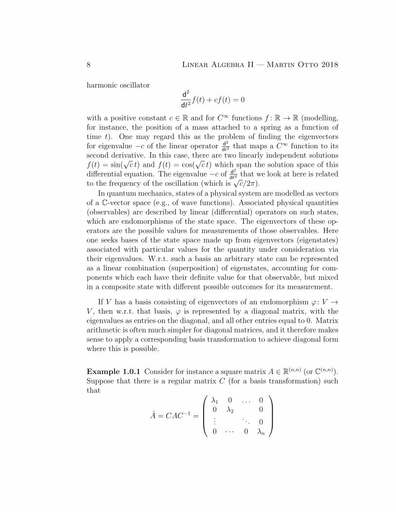
Example 1.0.1 Consider for instance a square matrix A ∈ R(n,n) (or C(n,n)).Suppose that there is a regular matrix C (for a basis transformation) suchthat
A = CAC−1 =
λ1 0 . . . 00 λ2 0...
. . . 00 · · · 0 λn
LA II — Martin Otto 2018 9
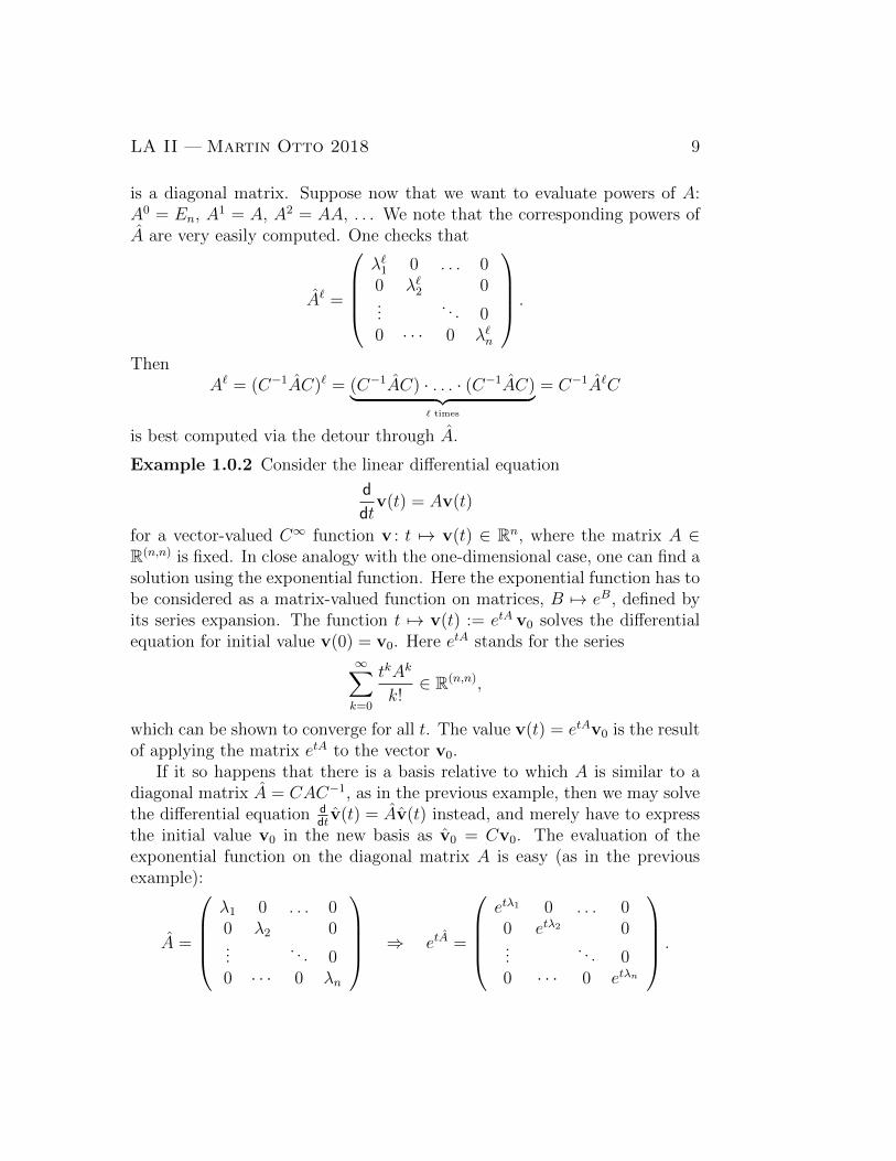
is a diagonal matrix. Suppose now that we want to evaluate powers of A:A0 = En, A1 = A, A2 = AA, . . . We note that the corresponding powers ofA are very easily computed. One checks that
A` =
λ`1 0 . . . 00 λ`2 0...
. . . 00 · · · 0 λ`n
.
ThenA` = (C−1AC)` = (C−1AC) · . . . · (C−1AC)︸ ︷︷ ︸
` times
= C−1A`C
is best computed via the detour through A.
Example 1.0.2 Consider the linear differential equation
d
dtv(t) = Av(t)
for a vector-valued C∞ function v : t 7→ v(t) ∈ Rn, where the matrix A ∈R(n,n) is fixed. In close analogy with the one-dimensional case, one can find asolution using the exponential function. Here the exponential function has tobe considered as a matrix-valued function on matrices, B 7→ eB, defined byits series expansion. The function t 7→ v(t) := etA v0 solves the differentialequation for initial value v(0) = v0. Here etA stands for the series
∞∑k=0
tkAk
k!∈ R(n,n),
which can be shown to converge for all t. The value v(t) = etAv0 is the resultof applying the matrix etA to the vector v0.
If it so happens that there is a basis relative to which A is similar to adiagonal matrix A = CAC−1, as in the previous example, then we may solvethe differential equation d
dtv(t) = Av(t) instead, and merely have to express
the initial value v0 in the new basis as v0 = Cv0. The evaluation of theexponential function on the diagonal matrix A is easy (as in the previousexample):
A =
λ1 0 . . . 00 λ2 0...
. . . 00 · · · 0 λn
⇒ etA =
etλ1 0 . . . 00 etλ2 0...
. . . 00 · · · 0 etλn
.
10 Linear Algebra II — Martin Otto 2018
We correspondingly find that the solution (in the adapted basis) is
v(t) = etA v0,
which then transforms back into the original basis according to
v(t) =[C−1etAC]v0.
Convention: in this chapter, unless otherwise noted, we fix a finite-dimen-sional F-vector space V of dimension greater than 0 throughout. We shalloccasionally look at specific examples and specify concrete fields F.
1.1 Eigenvectors and eigenvalues
Recall from chapter 3 in part I that Hom(V, V ) stands for the space of alllinear maps ϕ : V → V (vector space homomorphisms from V to V , i.e.,endomorphisms). Recall that w.r.t. to the natural addition and scalar mul-tiplication operations, Hom(V, V ) forms an F-vector space; while w.r.t. ad-dition and composition it forms a ring. This structure is isomorphic to thecorresponding structure on the space F(n,n) of all n × n matrices over F,which forms an F-vector space w.r.t. component-wise addition and scalarmultiplication; and a ring w.r.t. addition and matrix multiplication. Isomor-phisms between Hom(V, V ) and F(n,n) are induced by choices of bases for V .For any fixed labelled basis B = (b1, . . . ,bn) of V , the association betweenϕ ∈ Hom(V, V ) and A = [[ϕ]]BB provides a bijection that is compatible withall the above operations, and hence forms both a vector space isomorphismand a ring isomorphism.
Recall also from chapter 3 in part I how different choices of bases for V ,say B = (b1, . . . ,bn) and B = (b1, . . . , bn), induce different matrix represen-tations of endomorphisms. The relationship between the matrices A = [[ϕ]]BBand A = [[ϕ]]B
Bis governed by the regular change of basis matrix C and its
inverse C−1
A = CAC−1.
Here C = [[idV ]]BB
is the matrix representation of the identity w.r.t. bases B
in the domain and B in the range; C−1 correspondingly is [[idV ]]BB. Recall
LA II — Martin Otto 2018 11
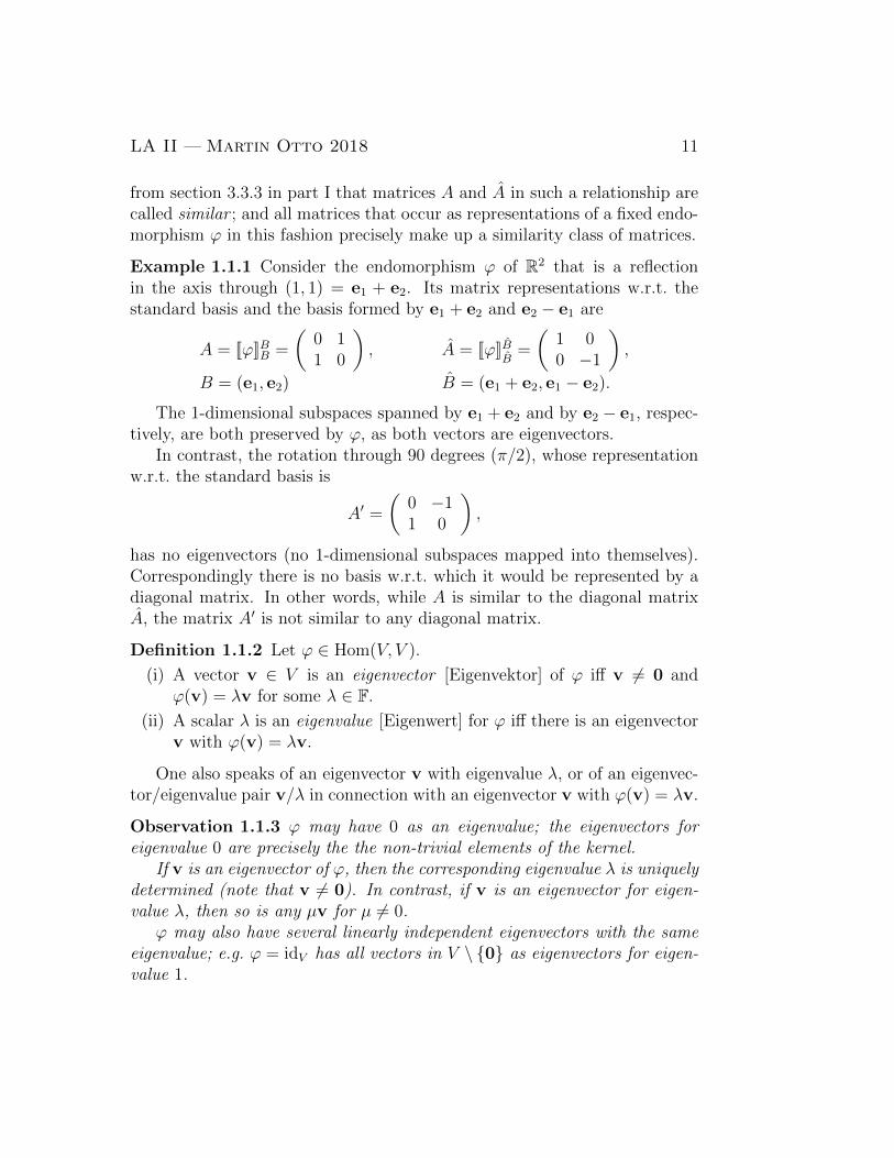
from section 3.3.3 in part I that matrices A and A in such a relationship arecalled similar ; and all matrices that occur as representations of a fixed endo-morphism ϕ in this fashion precisely make up a similarity class of matrices.
Example 1.1.1 Consider the endomorphism ϕ of R2 that is a reflectionin the axis through (1, 1) = e1 + e2. Its matrix representations w.r.t. thestandard basis and the basis formed by e1 + e2 and e2 − e1 are
A = [[ϕ]]BB =
(0 11 0
), A = [[ϕ]]B
B=
(1 00 −1
),
B = (e1, e2) B = (e1 + e2, e1 − e2).
The 1-dimensional subspaces spanned by e1 + e2 and by e2 − e1, respec-tively, are both preserved by ϕ, as both vectors are eigenvectors.
In contrast, the rotation through 90 degrees (π/2), whose representationw.r.t. the standard basis is
A′ =
(0 −11 0
),
has no eigenvectors (no 1-dimensional subspaces mapped into themselves).Correspondingly there is no basis w.r.t. which it would be represented by adiagonal matrix. In other words, while A is similar to the diagonal matrixA, the matrix A′ is not similar to any diagonal matrix.
Definition 1.1.2 Let ϕ ∈ Hom(V, V ).
(i) A vector v ∈ V is an eigenvector [Eigenvektor] of ϕ iff v 6= 0 andϕ(v) = λv for some λ ∈ F.
(ii) A scalar λ is an eigenvalue [Eigenwert] for ϕ iff there is an eigenvectorv with ϕ(v) = λv.
One also speaks of an eigenvector v with eigenvalue λ, or of an eigenvec-tor/eigenvalue pair v/λ in connection with an eigenvector v with ϕ(v) = λv.
Observation 1.1.3 ϕ may have 0 as an eigenvalue; the eigenvectors foreigenvalue 0 are precisely the the non-trivial elements of the kernel.
If v is an eigenvector of ϕ, then the corresponding eigenvalue λ is uniquelydetermined (note that v 6= 0). In contrast, if v is an eigenvector for eigen-value λ, then so is any µv for µ 6= 0.
ϕ may also have several linearly independent eigenvectors with the sameeigenvalue; e.g. ϕ = idV has all vectors in V \ {0} as eigenvectors for eigen-value 1.
12 Linear Algebra II — Martin Otto 2018
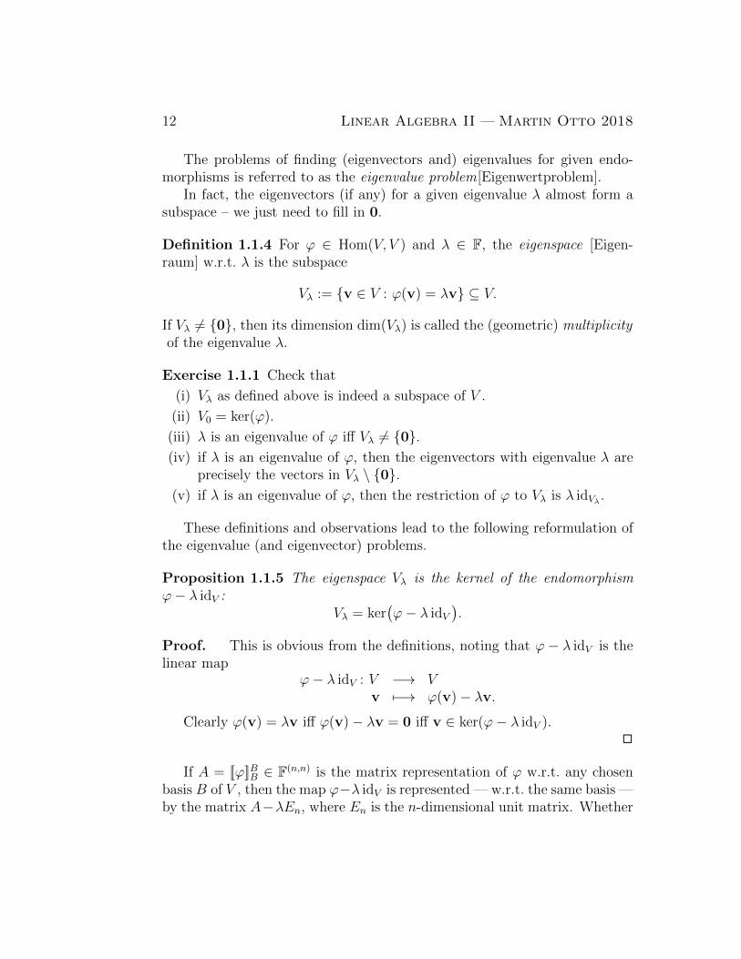
The problems of finding (eigenvectors and) eigenvalues for given endo-morphisms is referred to as the eigenvalue problem[Eigenwertproblem].
In fact, the eigenvectors (if any) for a given eigenvalue λ almost form asubspace – we just need to fill in 0.
Definition 1.1.4 For ϕ ∈ Hom(V, V ) and λ ∈ F, the eigenspace [Eigen-raum] w.r.t. λ is the subspace
Vλ := {v ∈ V : ϕ(v) = λv} ⊆ V.
If Vλ 6= {0}, then its dimension dim(Vλ) is called the (geometric) multiplicityof the eigenvalue λ.
Exercise 1.1.1 Check that
(i) Vλ as defined above is indeed a subspace of V .
(ii) V0 = ker(ϕ).
(iii) λ is an eigenvalue of ϕ iff Vλ 6= {0}.(iv) if λ is an eigenvalue of ϕ, then the eigenvectors with eigenvalue λ are
precisely the vectors in Vλ \ {0}.(v) if λ is an eigenvalue of ϕ, then the restriction of ϕ to Vλ is λ idVλ .
These definitions and observations lead to the following reformulation ofthe eigenvalue (and eigenvector) problems.
Proposition 1.1.5 The eigenspace Vλ is the kernel of the endomorphismϕ− λ idV :
Vλ = ker(ϕ− λ idV
).
Proof. This is obvious from the definitions, noting that ϕ − λ idV is thelinear map
ϕ− λ idV : V −→ Vv 7−→ ϕ(v)− λv.
Clearly ϕ(v) = λv iff ϕ(v)− λv = 0 iff v ∈ ker(ϕ− λ idV ).2
If A = [[ϕ]]BB ∈ F(n,n) is the matrix representation of ϕ w.r.t. any chosenbasis B of V , then the map ϕ−λ idV is represented — w.r.t. the same basis —by the matrix A−λEn, where En is the n-dimensional unit matrix. Whether
LA II — Martin Otto 2018 13
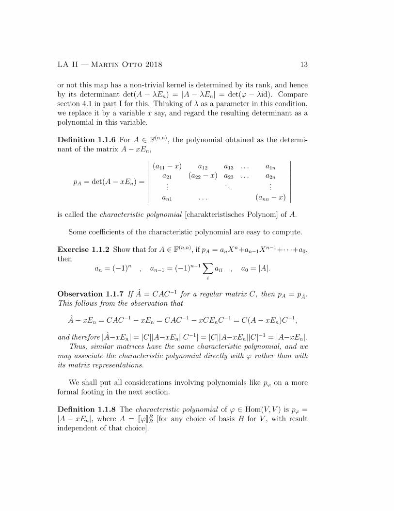
or not this map has a non-trivial kernel is determined by its rank, and henceby its determinant det(A − λEn) = |A − λEn| = det(ϕ − λid). Comparesection 4.1 in part I for this. Thinking of λ as a parameter in this condition,we replace it by a variable x say, and regard the resulting determinant as apolynomial in this variable.
Definition 1.1.6 For A ∈ F(n,n), the polynomial obtained as the determi-nant of the matrix A− xEn,
pA = det(A− xEn) =
∣∣∣∣∣∣∣∣∣(a11 − x) a12 a13 . . . a1na21 (a22 − x) a23 . . . a2n...
. . ....
an1 . . . (ann − x)
∣∣∣∣∣∣∣∣∣is called the characteristic polynomial [charakteristisches Polynom] of A.
Some coefficients of the characteristic polynomial are easy to compute.
Exercise 1.1.2 Show that for A ∈ F(n,n), if pA = anXn+an−1X
n−1+· · ·+a0,then
an = (−1)n , an−1 = (−1)n−1∑i
aii , a0 = |A|.
Observation 1.1.7 If A = CAC−1 for a regular matrix C, then pA = pA.This follows from the observation that
A− xEn = CAC−1 − xEn = CAC−1 − xCEnC−1 = C(A− xEn)C−1,
and therefore |A−xEn| = |C||A−xEn||C−1| = |C||A−xEn||C|−1 = |A−xEn|.Thus, similar matrices have the same characteristic polynomial, and we
may associate the characteristic polynomial directly with ϕ rather than withits matrix representations.
We shall put all considerations involving polynomials like pϕ on a moreformal footing in the next section.
Definition 1.1.8 The characteristic polynomial of ϕ ∈ Hom(V, V ) is pϕ =|A − xEn|, where A = [[ϕ]]BB [for any choice of basis B for V , with resultindependent of that choice].
14 Linear Algebra II — Martin Otto 2018
Theorem 1.1.9 For any ϕ ∈ Hom(V, V ) and λ ∈ F: λ is an eigenvalue ofϕ iff pϕ(λ) = 0, i.e., if λ is a zero of the characteristic polynomial pϕ.
Proof. Let B be any basis of V , and A = [[ϕ]]BB be the correspondingmatrix representation of ϕ. By the above, λ is an eigenvalue iff Vλ 6= {0} iffker(ϕ−λ idV ) 6= {0} iff A−λEn is not regular iff |A−λEn| = 0 iff pA(λ) = 0iff pϕ(λ) = 0.
2
Definition 1.1.10 Let ϕ ∈ Hom(V, V ). A subspace U ⊆ V is called aninvariant subspace for ϕ, or invariant under ϕ, if ϕ(u) ∈ U for all u ∈ U .
Observation 1.1.11 Any eigenspace Vλ of ϕ is an invariant subspace of ϕ.
Exercise 1.1.3 Consider a rotation in R3 through angle α about the axisspanned by a ∈ R3 \ {0} [w.l.o.g. fix a = e3]. Determine all all its invariantsubspaces
(i) for 0 < α < π.
(ii) for α = π.
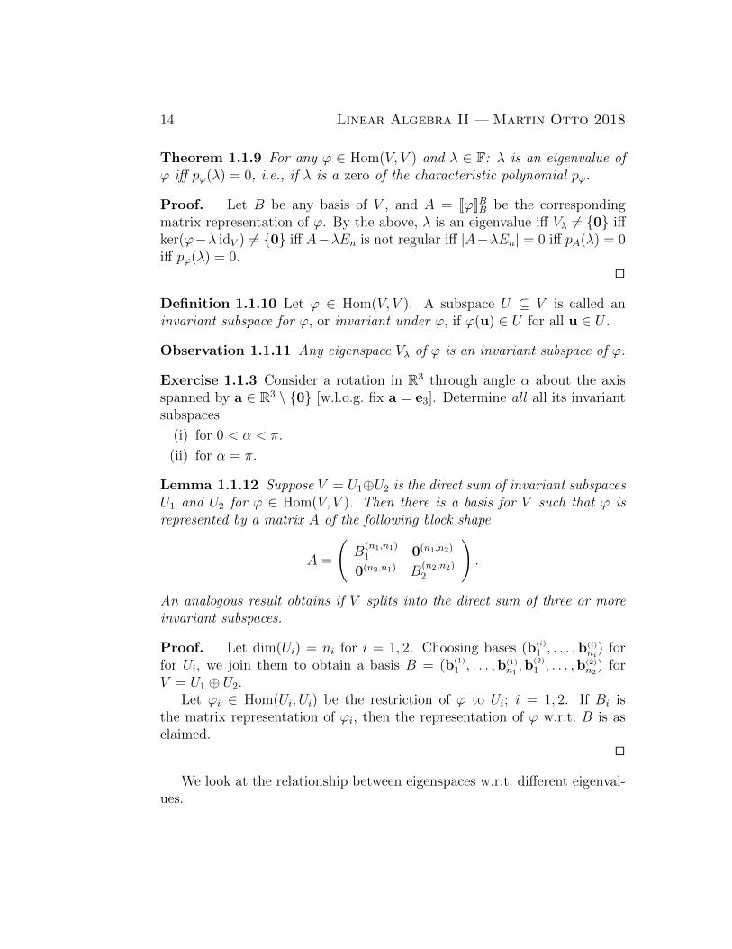
Lemma 1.1.12 Suppose V = U1⊕U2 is the direct sum of invariant subspacesU1 and U2 for ϕ ∈ Hom(V, V ). Then there is a basis for V such that ϕ isrepresented by a matrix A of the following block shape
A =
(B
(n1,n1)1 0(n1,n2)
0(n2,n1) B(n2,n2)2
).
An analogous result obtains if V splits into the direct sum of three or moreinvariant subspaces.
Proof. Let dim(Ui) = ni for i = 1, 2. Choosing bases (b(i)
1 , . . . ,b(i)ni
) forfor Ui, we join them to obtain a basis B = (b(1)
1 , . . . ,b(1)n1,b(2)
1 , . . . ,b(2)n2
) forV = U1 ⊕ U2.
Let ϕi ∈ Hom(Ui, Ui) be the restriction of ϕ to Ui; i = 1, 2. If Bi isthe matrix representation of ϕi, then the representation of ϕ w.r.t. B is asclaimed.
2
We look at the relationship between eigenspaces w.r.t. different eigenval-ues.
LA II — Martin Otto 2018 15
Proposition 1.1.13 Let ϕ ∈ Hom(V, V ) and suppose λ1, . . . , λm are distincteigenvalues of ϕ. Then the sum of the corresponding eigenspaces Vλi fori = 1, . . . ,m is direct, i.e., Vλ1 + Vλ2 + · · ·+ Vλm = Vλ1 ⊕ Vλ2 ⊕ · · · ⊕ Vλm.
Proof. By induction on m > 2. Consider the case of m = 2. We need toshow that Vλ1 ∩Vλ2 = {0}. Let v ∈ Vλ1 ∩Vλ2 . Then, as v ∈ Vλ1 , ϕ(v) = λ1v;and, as also v ∈ Vλ2 , ϕ(v) = λ2v. Hence λ1v = λ2v and (λ1 − λ2)v = 0. Asλ1 6= λ2, this implies v = 0.
The induction step is similar. Assume the claim is true for a sum of lessthan m distinct eigenspaces. We then show that also Vλ1 ∩
∑mi=2 Vλi = {0}.
Notice, that by the inductive hypotheses, we already have that∑m
i=2 Vλi =⊕mi=2 Vλi , which in particular implies that any v ∈
∑mi=2 Vλi has a unique
decomposition as v =∑m
i=2 ui with ui ∈ Vλi .So let v ∈ Vλ1 ∩
∑mi=2 Vλi . Then v =
∑mi=2 ui with ui ∈ Vλi and by
linearity, ϕ(v) =∑m
i=2 ϕ(ui) =∑m
i=2 λiui. On the other hand, as v ∈ Vλ1 ,ϕ(v) = λ1v. Hence
∑mi=2(λ1 − λi)ui = 0. Uniqueness of decompositions in⊕m
i=2 Vλi , applied to 0, implies that (λ1 − λi)ui = 0 for i = 2, . . . ,m, and asλi 6= λ1, it follows that the ui are all equal to 0. Therefore v = 0.
2
Remark 1.1.14 If dim(V ) = n, it follows that ϕ ∈ Hom(V, V ) can haveat most n distinct eigenvalues. This is because each eigenvalue λ gives riseto a non-trivial eigenspace Vλ 6= {0} of dimension dim(Vλ) > 1. As thesum of distinct eigenspaces is direct, the dimension of this sum is the sum oftheir dimensions. If ϕ has m distinct eigenvalues, therefore, the sum of thecorresponding eigenspaces has dimension at least m. So m 6 n follows.
We can already describe some cases in which ϕ ∈ Hom(V, V ) can bediagonalised , i.e., is represented by a diagonal matrix for a suitable choice ofbasis.
Proposition 1.1.15 Let dim(V ) = n. Then each one of the following con-ditions guarantees that there is a basis of V w.r.t. which ϕ is represented bya diagonal matrix (ϕ is diagonalisable):
(i) ϕ has n distinct eigenvalues.
(ii) pϕ has n distinct zeroes.
(iii) ϕ has m distinct eigenvalues λ1, . . . , λm such that∑m
i=1 dim(Vλi) = n.
16 Linear Algebra II — Martin Otto 2018
Proof. (i) and (ii) are equivalent by Theorem 1.1.9. Both describe aspecial case of condition (iii), namely where m = n and hence dim(Vλi) = 1.
So we concentrate on (iii). Firstly, the Vλi are invariant subspaces, andtheir direct sum is equal to V by the assumption about dimensions. ByLemma 1.1.12, it suffices to argue that the restriction ϕi of ϕ to Vλi admitsa diagonal representation. Any basis for Vλi will do, as by definition of Vλi ,ϕi = λi id is represented by λiEni if ni = dim(Vλi).
2
1.2 Polynomials
The role of the characteristic polynomial in connection with Theorem 1.1.9suggests that an algebraic understanding of polynomials in one variable holdsthe key to a more detailed analysis of diagonalisability. This section providesthe basis for this.
Definition 1.2.1 Let F be a field. A polynomial [Polynom] over F in onevariable X is a formal sum p =
∑mi=0 aiX
i with coefficients ai ∈ F. We writeF[X] for the set of all polynomials in variable X over F.
Convention: X0 is identified with 1 ∈ F, X1 with X, and any X i fori > 2 will be regarded as an m-fold product of X, once we endow F[X] witha multiplication operation. We speak of the exponent i in X i as the poweror order of X in that term. The coefficient ai in p =
∑mi=0 aiX
i is called thecoefficient of order or power i. The non-zero coefficient of the highest orderin p is called the leading coefficient [Leitkoeffizient] of p.
We identify all polynomials whose coefficients are all 0 (i.e., we do notdistinguish between 0, 0+0X, 0+0X+0X2, etc), and regard them as differentrepresentations of the null polynomial or zero polynomial, written just 0. Thenull polynomial is the only polynomial without a leading coefficient.
A polynomial is called normalised if it is the null polynomial or else if itsleading coefficient is 1.
Definition 1.2.2 The degree [Grad] of the polynomial p =∑m
i=0 aiXi ∈
F[X], denoted d(p) is the power of the leading coefficient, if p is not the nullpolynomial. For the null polynomial we put d(0) := −∞. 1
1This convention will have the advantage that it gives a degree to the null polynomialthat is smaller than that of any other polynomial (even up to addition of any n ∈ N).
LA II — Martin Otto 2018 17
Polynomials of degree 0 and the null polynomial, i.e., polynomials p =a0X
0 = a0 are called constant polynomials and identified with a0 ∈ F. Inthis way we regard F as a subset of F[X].
Polynomials of degree 1, p = a0 + a1X with a1 6= 0, are called linear ;those of degree 2, p = a0 + a1X + a2X
2 with a2 6= 0, quadratic; etc.
It is important to note that we do not identify a polynomial p =∑
i aiXi
in F[X] with the polynomial function
p : F −→ Fλ 7−→ p(λ) :=
∑i aiλ
i (∗)
which is an element of Pol(F) ⊆ F(F,F) (familiar as an F-vector space fromlast term).
In fact we need to keep the two notions separate, especially when dealingwith finite fields. We saw, for instance, that over F2 the polynomial functionsp(x) = x2 and p′(x) = x are the same; we do not, however, identify thepolynomials X and X2 in F2[X]. We shall see below that F[X] as well asPol(F) carry structure as F-vector spaces and as rings. With respect to bothstructures the association between formal polynomials and the polynomialfunctions they induce, is structure preserving in the sense of a (vector spaceor ring) homomorphism, but is not injective.
Consider, for instance, the F2-vector spaces Pol(F2) and F2[X]. Pol(F2) =F(F2,F2) has dimension 2 (four elements), but F2[X] will be infinite-dimen-sional. In particular, p0 = 1, p1 = X, p2 = X2, . . . , are all distinct and infact linearly independent in F2[X].
Exercise 1.2.1 Check thatˇ : F[X]→ Pol(F) is bijective for F = R, but notfor any Fp (p a prime).
We shall later look at evaluations of polynomials p ∈ F[X] not just overF, but also over the ring Hom(V, V ), or over the ring F(n,n). Writing p(ϕ) orp(A) (which give values to be defined below) we may regard these as values ofcorresponding ‘polynomial functions’ analogous to p but over domains otherthan F. Generally we shall suppress the p notation in all these cases and alsoreturn to writing just p(λ) for the value of p on argument λ.
1.2.1 Algebra of polynomials
Addition of polynomials. Addition of formal polynomials in F[X] is de-fined in component-wise fashion. If p =
∑mi=0 aiX
i and q =∑n
i=0 biXi, we
18 Linear Algebra II — Martin Otto 2018
may firstly assume that n = m by extending the polynomial of lower degreewith coefficients 0 as necessary. We then put
p+ q =( m∑i=0
aiXi)
+( m∑i=0
biXi)
:=m∑i=0
(ai + bi)Xi.
Note that d(p + q) 6 max(d(p), d(q)). The degree may indeed dropthrough cancellation of coefficients: in particular, if bi = −ai for all i, thenthey add up to the null polynomial.
In fact F[X] carries the structure of an F-vector space, with a corre-spondingly defined component-wise scalar multiplication. Since F ⊆ F[X]via constant polynomials, this multiplication may, however, also be consid-ered as a special case of the more general multiplication between polynomialsto be considered below.
Exercise 1.2.2 Define component-wise scalar multiplication similarly, andverify that this, together with addition, turns F[X] into an F-vector spacewith null vector 0 (the null polynomial).
Multiplication of polynomials. We define a multiplication operation onF[X] as follows. If p =
∑mi=0 aiX
i and q =∑n
i=0 biXi, we put
p · q =( m∑i=0
aiXi)( n∑
i=0
biXi)
:=m+n∑k=0
( ∑i+j=k
ai · bj)Xk.
Note that this multiplication gives what one would expect when applyingdistributivity and commutativity rules together with the obvious X iXj :=X i+j and re-grouping terms w.r.t. to orders Xk.
Observation 1.2.3 Multiplication of polynomials is additive w.r.t. degrees:d(pq) = d(p) + d(q).
In case at least one of p or q is the null polynomial, we extend the con-vention regarding d(0) = −∞ by the “natural” crutches that −∞ + n =n+ (−∞) = −∞+ (−∞) = −∞.
Proposition 1.2.4 (F[X],+, ·, 0, 1) forms a commutative ring with neutralelement 0 (the null polynomial) for addition, and neutral element 1 (theconstant polynomial 1) for multiplication.
LA II — Martin Otto 2018 19
Proof. Check the axioms, compare section 1.3.3 in part I.2
A scalar multiplication F× F[X]→ F[X] is obtained as the restriction ofthe above multiplication of polynomials to the case where the first polynomialis a constant polynomial p = a0 ∈ F.
Proposition 1.2.5 W.r.t. addition and the induced scalar multiplication ofpolynomials, F[X] forms an F-vector space with null vector 0 (the null poly-nomial).
Proof. Check the axioms.2
Proposition 1.2.6 The mapˇ : F[X]→ Pol(F) is compatible with the oper-ations of addition and multiplication and thus constitutes
(a) an F-vector space homomorphism w.r.t. to the vector space structure ofF[X] and Pol(F).
(b) a ring homomorphism w.r.t. to the ring structure of F[X] and Pol(F).
Exercise 1.2.3 Show that the F-vector space F[X] is infinite-dimensional,by showing that the pi = X i for i ∈ N are linearly independent.
Compare this with Pol(F), for instance for F = F2.
The following says that the product of two non-zero polynomials cannotbe zero in F[X]. Rings with this property are called integral domains [In-tegritatsbereiche]. That not all rings share this property, can be seen forinstance in Zq for q not a prime. Fields on the other hand always satisfy thiscondition (why?).
Proposition 1.2.7 For any p, q ∈ F[X]: pq = 0 ⇒ p = 0 or q = 0.
Proof. This is a consequence of Observation 1.2.3 on degrees under mul-tiplication. In more detail: suppose p, q 6= 0; then d(p), d(q) > 0 and thecorresponding coefficients ad(p) in p and bd(q) in q are both different from 0.Hence the coefficient of order d = d(p) +d(q), which is ad(p) · bd(q), is differentfrom zero, whence d(pq) > 0 and the product cannot be the null polynomial.
2
Exercise 1.2.4 Show that the only elements of F[X] that have an inversew.r.t. multiplication are the non-zero constant polynomials (i.e., those inF \ {0} ⊆ F[X]).
20 Linear Algebra II — Martin Otto 2018
1.2.2 Division of polynomials
An interesting topic in rings generally is divisibility . Over the familiar ring(Z,+, ·, 0, 1) of the integers, the investigation of divisibility gives rise to thenotions of division with remainder, greatest common divisors, and primenumbers, among others. We shall encounter similar notions in the ring F[X].
The ring F[X] fails to be a field (check that X ∈ F[X] does not havea multiplicative inverse). Therefore, the question of whether for given p, qthere is a polynomial r such that q · r = p is non-trivial.
We first define division with remainder for polynomials.
Definition 1.2.8 Let p, q ∈ F[X], q 6= 0. Then s ∈ F[X] is the result ofdividing p by q with remainder r ∈ F[X] if
p = sq + r where d(r) < d(q).
Lemma 1.2.9 For p, q ∈ F[X] as above, p can be divided by q with remain-der, with unique results s, r ∈ F[X].
Proof. We first consider the case that d(p) < d(q). Then s = 0 and r = pare admissible results. To see that they are uniquely determined, note that ifs 6= 0 then necessarily d(sq) > d(q). As d(r) < d(q) is a requirement, we findthat necessarily d(sq + r) = d(sq) > d(q) (look at the leading coefficients).But then d(sq + r) > d(p) shows that p 6= sq + r.
We now prove the general case by induction on d(p) > 0. The base case,for d(p) = 0, is easy. So we assume d(p) > 1 and that the claim has beenestablished for all p′ of degree less than n = d(p). If d(q) > n we are doneby the above. So let d(q) := m 6 n. Let p =
∑ni=0 aiX
i and q =∑m
j=0 bjXj.
If p = sq + r with d(r) < d(q) then d(s) must be k := n −m. So we knowthat any result must be of the form s = ckX
k + s′ where d(s′) < k, ck 6= 0.
Now sq + r = (ckXk + s′)q + r has leading coefficient ckbm of order
m + k = n. Necessarily therefore ck = an/bm. The task of finding s and rsuch that p = sq + r with d(r) < d(q) now reduces to finding s′ and r′ suchthat p′ = s′q + r′ with d(r′) < d(q) for p′ = p − (an/bm)Xkq. Since p′ is apolynomial of degree d(p′) < n, there is a unique solution according to theinductive hypothesis.
2
LA II — Martin Otto 2018 21
Definition 1.2.10 For p, q ∈ F[X], q 6= 0: q divides p, denoted q|p, iffp = sq for some s ∈ F[X] (with remainder 0). We explicitly also include thecase where p = 0: any non-zero polynomial divides the null polynomial 0. Apolynomial that divides p is called a divisor.
We do not regard the null polynomial as a divisor of any polynomial.
Note that whenever q divides p then so does cq for any c ∈ F\{0}: divisorsare best considered up to multiplication with non-zero constant polynomialsbecause divisibility in the field F is trivial.
Exercise 1.2.5 Show for p, q ∈ F[X]: if p|q and q|p then p and q are constantmultiples of each other, i.e., p = cq and q = c−1p for some c ∈ F \ {0}. Hint:look at the degrees.
We now link divisibility by simple degree 1 polynomials (linear factors,roots) to the existence of zeroes. While zeroes are defined in terms of theassociated polynomial function, we thus link them to divisibility in F[X].
Definition 1.2.11 Let p ∈ F[X] and λ ∈ F.
(i) λ ∈ F is a zero [Nullstelle] of p iff p(λ) = 0.
(ii) p has the linear factor [Linearfaktor] (X−λ), or p has the root [Wurzel]λ, iff (X − λ) divides p, i.e., iff p = (X − λ)s for some s ∈ F[X].
(iii) If λ is a root of p, then the algebraic multiplicity of λ is the maximalm such that (X − λ)m divides p.
Proposition 1.2.12 For p ∈ F[X] of degree at least 1, and for any λ ∈ F:λ is a zero of p iff p has (X − λ) as a linear factor.
Proof. Clearly, if p = (X−λ)s, then p(x) = (x−λ)s(x) and thus p(λ) = 0.Conversely, assume that p(λ) = 0. As d(p) > 1, we may divide p by
q = (X − λ) with remainder: p = (X − λ)s + r where d(r) < 1 means thatr ∈ F. Hence p(x) = (x − λ)s(x) + r and p(λ) = r. So r = 0 as λ is a zeroof p, and therefore (X − λ) divides p.
2
Exercise 1.2.6 Determine for which λ ∈ R the linear factor X − λ dividesthe polynomial p = X3 + 2X2 + 4X + 8 ∈ R[X]. One way of doing this isto compare coefficients in p and (X − λ)(X2 +αX + β) and making suitablecase distinctions regarding possible values for α, β, λ.
22 Linear Algebra II — Martin Otto 2018
Primes are numbers that are not non-trivially divisible, or numbers thatare irreducible by integer division. Irreducible polynomials are similarly de-fined. Trivial divisibility here concerns products involving a constant poly-nomial.
Definition 1.2.13 A polynomial p of degree p > 1 is called irreducible [ir-reduzibel] iff it is not divisible by any polynomial q of degree 0 < d(q) < p.
Example 1.2.14 Any degree 1 polynomial, and in particular any linear fac-tor (X − λ), is irreducible.
Example 1.2.15 Over the real field R, there are also irreducible polynomi-als of degree 2, like p = X2 + 1. The same polynomial is reducible whenviewed as a polynomial over the field C: X2 + 1 = (X − i)(X + i) in C[X].Any polynomial of odd degree over R has a zero (its graph crosses the x-axis) and hence, by the last Proposition, is divisible by a linear factor; henceany polynomial of odd degree greater than 1 over R is reducible. More onirreducibility in C[X] and R[X] is presented in section 1.2.3 below.
Exercise 1.2.7 Consider F2[X]. Show that any non-linear polynomial
(i) without the constant term 1, or
(ii) with an odd number of powers X i for i > 1 (with or without theconstant term 1)
is reducible in F2[X]. Find all irreducible polynomials of degree up to 4.[Note that all irreducible polynomials must describe the constant polynomialfunction 1, which is represented not just by the constant polynomial 1.]
The following notion is helpful in analysing divisibility questions in rings.
Definition 1.2.16 Let (A,+, ·, 0, 1) be a commutative ring. A non-emptysubset I ⊆ A is an ideal [Ideal] if it is closed under addition and undermultiplication with arbitrary ring elements:
(i) a, b ∈ I ⇒ a+ b ∈ I.
(ii) a ∈ I, r ∈ A ⇒ ra ∈ I.
An ideal I ⊆ A is a principal ideal [Hauptideal] if I = Ia := {ra : r ∈ A}consists of all the multiples of a fixed element a (the generator of I).
LA II — Martin Otto 2018 23
Proposition 1.2.17 Any ideal I ⊆ F[X] is a principal ideal, i.e., every idealI in F[X] possesses a generator p such that I = Ip = {pr : r ∈ F[X]}. Suchp is uniquely determined by I up to multiplication by constants c ∈ F; inparticular there is a unique normalised p such that I = Ip.
Proof. Let I ⊆ F[X] be an ideal. If I = {0}, then 0 generates I.Otherwise let p ∈ I be an element of minimal degree in I \{0}. We claim
that I = Ip for any such p ∈ I. Clearly Ip ⊆ I, as I is closed under arbitraryproducts with polynomials.
Let us show that I ⊆ Ip. Let q ∈ I. We may assume that q 6= 0 as 0 ∈ Ipanyway. We may divide q by p with remainder, q = ps+ r with d(r) < d(p).But r = q − ps ∈ I, and hence d(r) < d(p) implies that r = 0 by the choiceof p, and hence q ∈ Ip.
For uniqueness up to constants: if I 6= {0} and I = Ip = Iq then p|q andq|p imply that they are constant multiples of each other.
2
Definition 1.2.18 A greatest common divisor of two polynomials r, s ∈F[X] is any polynomial p ∈ F[X] such that p|r, p|s and for any other q ∈ F[X]that divides both r and s we have q|p. If the constant polynomial 1 is agreatest common divisor of r and s, then r and s are called relatively prime[teilerfremd].
Exercise 1.2.8 Show that any two distinct linear factors (X−λ1) and (X−λ2) in F[X] are relatively prime.
Lemma 1.2.19 Any two non-constant polynomials possess a greatest com-mon divisor q. This greatest common divisor r is unique up to multiplicationby constants c ∈ F \ {0}. If p is a greatest common divisor of s, t, thenp = gs+ ht for suitable g, h ∈ F[X].
Proof. For given s, t consider I := {gs + ht : g, h ∈ F[X]}. One checksthat I ⊆ F[X] is an ideal. By the previous lemma, I = Ip for some p ∈ F[X].We show that this p is a greatest common divisor of s and t.
Clearly p|s and p|t as s, t ∈ I = Ip. If q|s and q|t then, by distributivity,q divides any element gs+ ht of I, hence in particular also p.
For uniqueness up to constant factors, observe that any two greatestcommon divisors must divide each other.
2
24 Linear Algebra II — Martin Otto 2018
A fundamental property of primes with respect to (integer) divisibility isthat if a prime divides a product of two numbers then it must divide at leastone of those factors. A similar phenomenon obtains here.
Proposition 1.2.20 Let q be irreducible, q, r, s ∈ F[X]. If q divides rs thenq divides r or q divides s.
Proof. Let q be irreducible and assume that q divides rs, w.l.o.g., rs 6= 0.As q is irreducible it is not constant, therefore at least one of r and s mustalso be non-constant. W.l.o.g. assume that d(s) > 1. Let p be a greatestcommon divisor of s and q. From the last lemma we know that p is of theform p = gs+ hq for suitable g, h ∈ F[X].
As p|q there is t ∈ F[X] such that q = pt. But as q is irreducible, eitherp or t must be constant.
If t = c is constant, then q|p and hence q|s.If p = c is constant, then c = gs+ hq for suitable g, h ∈ F[X]. Therefore
1 = (c−1g)s + (c−1h)q and r = 1r = (c−1g)rs + (c−1h)qr is divisible by q,since rs and qr are both divisible by q.
2
Remark 1.2.21 From the above, one can conclude that similar to the primedecomposition in the ring of integers, the ring F[X] admits (an essentiallyunique) decomposition into irreducible polynomials. Any polynomial p ∈F[X]\{0} has a representation as a product of irreducible polynomials. Thisdecomposition is unique up to permutations and up to constants.
1.2.3 Polynomials over the real and complex numbers
What can we say about roots (or zeroes) of polynomials in F[X]? The answerlargely depends on F. We collect the crucial facts for the familiar classicalfields of the real and complex numbers, R and C. These results go beyondthe scope of this course.
Theorem 1.2.22 (Fundamental theorem of algebra)Any non-constant polynomial in C[X] has a zero. Consequently, any non-constant polynomial p ∈ C[X] of degree d(p) = n > 1 splits into linear factorsp = z0(X − z1) · · · (X − zn) for constants zi ∈ C.
LA II — Martin Otto 2018 25
The first statement implies the second, via Proposition 1.2.12 and induc-tion on the degree n.
Over R the situation is different. There are polynomials without zeroes,of any even degree. For instance, p = (X2 + 1)m has degree n = 2m and nozeroes. Any non-constant polynomial of odd degree, on the other hand, doeshave a zero and hence is divisible by a corresponding linear factor. [Thiscan be derived via the intermediate value theorem, but also follows along thelines of the algebraic argument given below.] It turns out that the irreduciblepolynomials in R[X] are precisely the linear factors (of degree 1) and thosedegree 2 polynomials without zeroes, viz. the constant multiples of quadraticpolynomials p = X2 + bX + c = (X + b/2)2 + (c− b2/4) for which c > b2/4.
Theorem 1.2.23 The irreducible polynomials in R[X] are precisely the lin-ear polynomials and those quadratic polynomials that have no zeroes.
The argument that any other non-constant real polynomial is reducibleessentially follows from Theorem 1.2.22. Using Proposition 1.2.12 it remainsto show that no polynomial p of even degree n = 2m > 2 is irreducible. Forthis we consider R[X] as a subset R[X] ⊆ C[X]. Over C, p splits into linearfactors. Up to a constant factor, p = (X − z1) · · · (X − zn) for zi ∈ C. Butbecause p ∈ R[X], p = p where p is obtained by complex conjugation of allcomplex numbers in p, sending zj = xj + iyj to zj = xj − iyj. It thereforefollows that all roots zj 6∈ R of p come in complex conjugate pairs, i.e., pis a product of real linear factors and pairs of complex linear factors of theform (X − z)(X − z). Any such pair, however, is still also a real polynomialof degree 2. If z = x + iy then (X − z)(X − z) = X2 − (z + z)X + zz =X2− 2xX + (x2 + y2) ∈ R[X]. I.e., p splits into polynomials of degree 2 evenin R[X]. Some of these may indeed be irreducible over R.
1.3 Upper triangle form
The irreducible factors of the characteristic polynomial determine whether ϕcan be represented by an upper triangle matrix or not.
A matrix A = (aij) ∈ F(n,n) is an upper triangle matrix if aij = 0 for1 6 j < i 6 n. This means that all non-zero entries are on the diagonal orabove. [An echelon matrix is a special case of an upper triangle matrix.]
Proposition 1.3.1 The following are equivalent for ϕ ∈ Hom(V, V ) withcharacteristic polynomial pϕ:
26 Linear Algebra II — Martin Otto 2018
(i) pϕ splits into linear factors.
(ii) there is a basis for V such that ϕ is represented by an upper trianglematrix A.
Note in particular, that by the fundamental theorem of algebra, any en-domorphism of a C-vector space admits a representation by an upper trianglematrix.
Proof. (ii)⇒ (i) is straightforward from the definition of pϕ(x) = pA(x) =|A − xEn|. Recall that the determinant of an upper triangle matrix equalsthe product of the diagonal entries, in this case of the linear factors (aii−X).
For (i)⇒ (ii) we proceed by induction on the dimension n of V . The caseof n = 1 is trivial.
For the induction step, assume n > 1 and that the claim is true in di-mension n− 1.
Let (X − λ) be a linear factor of p = pϕ, p = (X − λ)p′. As λ is a zeroof pϕ, there is an eigenvector b1 with eigenvalue λ: ϕ(b1) = λb1. We chooseb1 as our first basis vector.
Extending to a basis B = (b1,b2, . . . ,bn) of V , we obtain a matrix repre-sentation A = [[ϕ]]BB in which a11 = λ and all other entries in the first columnequal to 0.
A = [[ϕ]]BB =
λ a12 . . . a1n0... A′
0
Let V ′ = span(b2, . . . ,bn) and V1 = span(b1) so that V = V1 ⊕ V ′. Note
that B′ = (b2, . . . ,bn) is a basis for V ′.Define auxiliary linear maps ϕ′ ∈ Hom(V ′, V ′) and ψ ∈ Hom(V ′, V1)
as follows. For v ∈ V ′, the vector ϕ(v) ∈ V = V1 ⊕ V ′ has a uniquedecomposition into a sum of vectors from V1 and V ′, respectively. Define ϕ′
and ψ such that for v ∈ V ′:
ϕ(v) = ψ(v) + ϕ′(v) where ψ(v) ∈ V1 and ϕ′(v) ∈ V ′.
One checks that ϕ′ and ψ are indeed linear. W.r.t. basis B′ of V ′, ϕ′ isrepresented by the matrix A′ which is A with first row and first columnremoved.
LA II — Martin Otto 2018 27
If we expand pϕ(x) = |A − xEn| w.r.t. the first column, we find thatpϕ = (λ−X)p′, with p′ = pA′ = pϕ′ the characteristic polynomial of ϕ′.
Now p′ splits into linear factors since p = (X−λ)p′ does. By the inductivehypothesis, V ′ has a basis (b′2, . . . ,b
′n) w.r.t. which ϕ′ is represented by an
upper triangle matrix. In terms of ϕ′ and the b′i this means that for 2 6 i 6 n:
ϕ′(b′i) ∈ span(b′2, . . . ,b′i).
Finally the basis (b1,b′2, . . . ,b
′n) is a basis for V that is as desired for ϕ.
Indeed, for i = 1, ϕ(b1) = λb1 ∈ span(b1); and for 2 6 i 6 n,
ϕ(b′i) = ϕ′(b′i) +ψ(b′i) ∈ span(b′2, . . . ,b′i) + span(b1) = span(b1,b
′2, . . . ,b
′i).
2
Remark: In the situation of the induction step, the auxiliary map ϕ′ canbe found as a quotient map. Let U be the one-dimensional subspace U =span(v1). Then an alternative view of ϕ′ is as the map
ϕ′ : V/U −→ V/Uv + U 7−→ ϕ(v) + U.
One checks that this map is well defined, and corresponds to the above via anisomorphism of V/U = (V ′ ⊕ U)/U with V ′. Compare section 2.6 in part I.
Corollary 1.3.2 Let V be an n-dimensional C-vector space, ϕ∈ Hom(V, V ).Then there is a basis B for V such that ϕ is represented by an upper trianglematrix A w.r.t. to B.
The situation is obviously very different over R. We again look at thesimple example of a rotation through π/2 in R2. As this map does not havea single eigenvector, there is no first basis vector for achieving triangle form.
1.4 The Cayley–Hamilton Theorem
The Cayley–Hamilton Theorem is one of the key results in the analysis ofeigenvalues and eigenspaces. It makes a surprising connection between thecharacteristic polynomial pϕ ∈ F[X], whose zeroes are the eigenvalues, with
28 Linear Algebra II — Martin Otto 2018
the linear map that we obtain when we substitute ϕ itself for X in pϕ, or Afor X in pϕ where A is a matrix representation of ϕ. .
So far we have thought of evaluating polynomials p ∈ F[X] over F — thisis precisely what p : F → F stood for. But it also makes sense to evaluatea polynomial p ∈ F[X] on an endomorphism of an F-vector space or on asquare matrix over F. The required operations of scalar multiplication (ofmatrices or endomorphisms), of multiplication (of matrices) or composition(of endomorphisms), and of addition (of matrices or endomorphisms) are welldefined, and moreover obey the familiar laws of arithmetic in a ring.
Remark 1.4.1 The rings Hom(V, V ) or F(n,n) are not commutative — ingeneral we cannot expect that ϕ ◦ ψ = ψ ◦ ϕ or that AB = BA. We shallhere not notice this lack of commutativity, because we shall always workw.r.t. a fixed endomorphism ϕ (or matrix A) and its powers, because welook at polynomials in a single variable. All the ring arithmetic we shallencounter, therefore, takes place within sub-rings of the form{
p(ϕ) : p ∈ F[X]}⊆ Hom(V, V )
or{p(A) : p ∈ F[X]
}⊆ F(n,n).
In restriction to these, composition and matrix multiplication, respectively,are commutative.
Definition 1.4.2 Let V be an F-vector space. The evaluation map for poly-nomials p ∈ F[X] on Hom(V, V ) is defined to be compatible with the ringarithmetic of F[X] and Hom(V, V ), based on the following:
p(ϕ) = 0 (null endomorphism) for p = 0 (null polynomial)p(ϕ) = c idV for p = c ∈ F (a constant polynomial)p(ϕ) = ϕ for p = X.
Similarly, for the evaluation map on matrices in F(n,n), based on
p(A) = 0 (null matrix) for p = 0p(A) = cEn for p = c ∈ Fp(A) = A for p = X.
Note that the extension to arbitrary polynomials p ∈ F[X] is uniquelydetermined by these stipulations and the requirement of compatibility with
LA II — Martin Otto 2018 29
the ring structure. For instance, consider p = aX3 + bX + c for a, b, c ∈ F. Ifϕ ∈ Hom(V, V ), then p(ϕ) = a idV ◦ϕ◦ϕ◦ϕ+b idV ◦ϕ+c idV = aϕ3+bϕ+c idV ;and if A ∈ F(n,n), then p(A) = aEnAAA+ bEnA+ cEn = aA3 + bA+ cEn.
Moreover, if A happens to be the matrix representation of ϕ w.r.t. tosome basis B of V , then p(A) is the matrix representation, w.r.t. to B, ofp(ϕ).
Exercise 1.4.1 Check the last compatibility claim systematically by ver-ifying it first for the basic cases (null and constant polynomials, and thepolynomial X) and then showing that it is preserved under multiplicationand addition of polynomials.
Before we proceed to the main theorem and its proof, we recall an im-portant fact about matrices and determinants from last term, and convinceourselves that it lifts to the level of ring arithmetic in F[X] we need here.
Recall from chapter 4 in part I the matrices A[ij] obtained by deleting rowi and column j in A ∈ F(n,n). We used the determinants of these (up to a+/− sign) as the coefficients in a matrix A′ towards the construction of theinverse of A. More precisely, the coefficient in row i and column j of A′ was
a′ij = (−1)i+j|A[ji]|.
For this matrix we showed that
AA′ = A′A = |A|En.
Looking at the proof, which was just a calculation based on multilinearityand antisymmetry of the determinant, we see that the same identity alsoobtains if the matrices involved have entries from some commutative ringrather than from a field. Up to that point we had had no occasion to usemultiplicative inverses. (Of course, in order to obtain the inverse A−1 =|A|−1A′ in the case of a regular matrix A we did work over a field.) We shalluse the following in the proof of the Cayley–Hamilton Theorem below.
Observation 1.4.3 Define the determinant function on n×n matrices overa commutative ring by the familiar
∑σ∈Sn sign(σ) · · · formula. Consider a
matrix A over that ring with coefficients aij, 1 6 i, j 6 n, from that ring,and let, for 1 6 i, j 6 n,
a′ij = (−1)i+j|A[ji]|.
30 Linear Algebra II — Martin Otto 2018
Then, for 1 6 i, j 6 n:
n∑k=1
aika′ki = |A| and
n∑k=1
aika′kj = 0 for i 6= j.
Exercise 1.4.2 Review the proof of the corresponding fact over a field F, insection 4.2 of part I, and transfer it to the current situation. Discuss whethercommutativity is essential.
Theorem 1.4.4 (Cayley–Hamilton Theorem) Let pϕ be the character-istic polynomial of ϕ ∈ Hom(V, V ). Then
pϕ(ϕ) = 0 (the null endomorphism).
Similarly, for A ∈ F(n,n) with characteristic polynomial pA:
pA(A) = 0 (the null matrix).
Proof. The two statements are equivalent. We look at the matrix formu-lation. Let pA =
∑nj=0 αjX
j.Recall that pA = |A − XEn|. Let C = A − XEn be the matrix with
entries
aij − δijX
in row i and column j, where δij = 1 for i = j and 0 otherwise. Note that Chas entries in F[X]. Let C ′ be the related matrix whose entry in row i andcolumn j is
(−1)i+j|C[ji]|,
where the determinant is evaluated in the ring F[X] (!). By Observation 1.4.3above,
(A−XEn)C ′ = CC ′ = |C|En = pAEn.
Note that any entry (−1)i+j|C[ji]| in C ′ is a polynomial of degree less thann, since C[ji] is an (n− 1)× (n− 1) matrix whose entries are polynomials ofdegree up to 1. One may therefore expand C ′ in terms of powers of X in theform
C ′ =n−1∑i=0
DiXi,
LA II — Martin Otto 2018 31
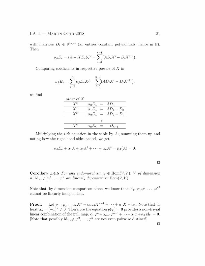
with matrices Di ∈ F(n,n) (all entries constant polynomials, hence in F).Then
pAEn = (A−XEn)C ′ =n−1∑i=0
(ADiXi −DiX
i+1).
Comparing coefficients in respective powers of X in
pAEn =n∑j=0
αjEnXj =
n−1∑i=0
(ADiXi −DiX
i+1),
we findorder of X
X0 α0En = AD0
X1 α1En = AD1 −D0
X2 α2En = AD2 −D1
......
Xn αnEn = −Dn−1
Multiplying the i-th equation in the table by Ai, summing them up andnoting how the right-hand sides cancel, we get
α0En + α1A+ α2A2 + · · ·+ αnA
n = pA(A) = 0.
2
Corollary 1.4.5 For any endomorphism ϕ ∈ Hom(V, V ), V of dimensionn: idV , ϕ, ϕ
2, . . . , ϕn are linearly dependent in Hom(V, V ).
Note that, by dimension comparison alone, we know that idV , ϕ, ϕ2, . . . , ϕn
2
cannot be linearly independent.
Proof. Let p = pϕ = αnXn + αn−1X
n−1 + · · · + α1X + α0. Note that atleast αn = (−1)n 6= 0. Therefore the equation p(ϕ) = 0 provides a non-triviallinear combination of the null map, αnϕ
n+αn−1ϕn−1+· · ·+α1ϕ+α0 idV = 0.
[Note that possibly idV , ϕ, ϕ2, . . . , ϕn are not even pairwise distinct!]
2
32 Linear Algebra II — Martin Otto 2018
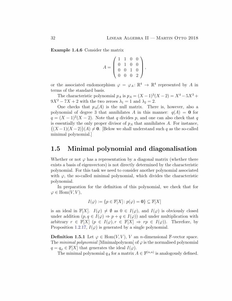
Example 1.4.6 Consider the matrix
A =
1 1 0 00 1 0 00 0 1 00 0 0 2
,
or the associated endomorphism ϕ = ϕA : R4 → R4 represented by A interms of the standard basis.
The characteristic polynomial pA is pA = (X − 1)3(X − 2) = X4− 5X3 +9X2 − 7X + 2 with the two zeroes λ1 = 1 and λ2 = 2.
One checks that pA(A) is the null matrix. There is, however, also apolynomial of degree 3 that annihilates A in this manner: q(A) = 0 forq = (X − 1)2(X − 2). Note that q divides p, and one can also check that qis essentially the only proper divisor of pA that annihilates A. For instance,((X−1)(X−2)
)(A) 6= 0. [Below we shall understand such q as the so-called
minimal polynomial.]
1.5 Minimal polynomial and diagonalisation
Whether or not ϕ has a representation by a diagonal matrix (whether thereexists a basis of eigenvectors) is not directly determined by the characteristicpolynomial. For this task we need to consider another polynomial associatedwith ϕ, the so-called minimal polynomial, which divides the characteristicpolynomial.
In preparation for the definition of this polynomial, we check that forϕ ∈ Hom(V, V ),
I(ϕ) := {p ∈ F[X] : p(ϕ) = 0} ⊆ F[X]
is an ideal in F[X]. I(ϕ) 6= ∅ as 0 ∈ I(ϕ), and I(ϕ) is obviously closedunder addition (p, q ∈ I(ϕ) ⇒ p + q ∈ I(ϕ)) and under multiplication witharbitrary r ∈ F[X] (p ∈ I(ϕ), r ∈ F[X] ⇒ rp ∈ I(ϕ)). Therefore, byProposition 1.2.17, I(ϕ) is generated by a single polynomial.
Definition 1.5.1 Let ϕ ∈ Hom(V, V ), V an n-dimensional F-vector space.The minimal polynomial [Minimalpolynom] of ϕ is the normalised polynomialq = qϕ ∈ F[X] that generates the ideal I(ϕ).
The minimal polynomial qA for a matrix A ∈ F(n,n) is analogously defined.
LA II — Martin Otto 2018 33
The following is essentially a corollary of the Cayley–Hamilton Theorem.
Proposition 1.5.2 The minimal polynomial qϕ divides the characteristicpolynomial pϕ. They have the same zeroes (roots) but possibly the algebraicmultiplicity of some roots is smaller in qϕ.
Proof. qϕ|pϕ follows from the definition and the fact that pϕ ∈ I byCayley–Hamilton.
Any root in qϕ gives rise to an irreducible linear factor which must there-fore also be a linear factor in pϕ, compare Proposition 1.2.20.
Conversely, a root λ of pϕ is an eigenvalue of ϕ. For a correspondingeigenvector v we have ϕk(v) = λkv. As (qϕ(ϕ))(v) = (qϕ(λ idV ))(v) = 0,this implies qϕ(λ) = 0. Hence λ is a zero of qϕ as well.
2
The following shows that, as far as upper triangle presentations are con-cerned, the minimal polynomial holds the same information as the charac-teristic polynomial, compare Proposition 1.3.1.
Proposition 1.5.3 Suppose ϕ ∈ Hom(V, V ) is such that its minimal poly-nomial qϕ splits into linear factors. Then ϕ is representable by an uppertriangle matrix.
Proof. The proof is very similar to the corresponding part of the proofof Proposition 1.3.1, and we discuss only the crucial variations.
If qϕ splits into linear factors, then pϕ also has a linear factor, and hencean eigenvector v1. We split V as V = U ⊕ V ′, where U = span(v1). Inorder to piece together the desired representation, we want to find a suitablerepresentation for ϕ over V ′, ignoring any components in U . We thereforeconsider the quotient V/U and the quotient map
ϕ′ : V/U −→ V/Uv + U 7−→ ϕ(v) + U.
As the quotient V/U = (U ⊕ V ′)/U is isomorphic to V ′, we may thereforeidentify ϕ′ with an endomorphism of V ′. In order to apply the inductivehypothesis to ϕ′ ∈ Hom(V ′, V ′) (or Hom(V/U, V/U)), we need that also qϕ′
splits into linear factors.
34 Linear Algebra II — Martin Otto 2018
This follows, as qϕ′|qϕ. One checks that for any polynomial r ∈ F[X] andv ∈ V :
[r(ϕ′)](v + U) = [r(ϕ)](v) + U.
In particular, [qϕ(ϕ′)](v +U) = [qϕ(ϕ)](v) +U = 0+U shows that qϕ(ϕ′)is the null map. Therefore, qϕ′ |qϕ, and qϕ′ must also split into linear factors.
The rest of the argument, i.e., the piecing together of an upper trianglerepresentation of ϕ′ for a suitable basis of V ′ with the extra basis vector v1,is exactly as in the proof of Proposition 1.3.1.
2
Combining this with Proposition 1.3.1, we obtain the following.
Corollary 1.5.4 For any ϕ ∈ Hom(V, V ): pϕ splits into linear factors iff qϕsplits into linear factors.
We link the minimal polynomial to diagonalisability of endomorphisms(matrices). This further clarifies the situation which was partially describedin Proposition 1.1.15 above.
Lemma 1.5.5 If ϕ ∈ Hom(V, V ) is diagonalisable, i.e., if V has a basisconsisting of eigenvectors of ϕ, then qϕ splits into linear factors of algebraicmultiplicity 1: qϕ =
∏mi=1(X − λi) if λ1, . . . , λm are the pairwise distinct
eigenvalues of ϕ.
Proof. It suffices to show that q(ϕ) = 0 for q =∏m
i=1(X − λi), since thereal qϕ divides any such q and must have these zeroes. (The point is that nohigher multiplicities are necessary.)
Let B be a basis of eigenvectors, b ∈ B an eigenvector with eigenvalueλi. Writing q =
∏mj=1(X − λj) as q = (X − λi)q′i = q′i(X − λi), we see that
q(ϕ) = (q′i(ϕ)) ◦ (ϕ− λi idV ). Hence (q(ϕ))(b) = (q′i(ϕ))(0) = 0.
Since this argument carries through for every basis vector in B, q(ϕ) isindeed the null map.
2
Towards the converse of the lemma, we look at products of polynomialsthat are relatively prime.
LA II — Martin Otto 2018 35
Lemma 1.5.6 Let q1, . . . , qm ∈ F[X] be relatively prime. If q =∏m
i=1 qi then
ker(q(ϕ)) =m⊕i=1
ker(qi(ϕ)).
Proof. We consider the case of two factors. Let q = q1q2.
The inclusions ker(qi(ϕ)) ⊆ ker(q(ϕ)) are easy. For instance, for v ∈ker(qi(ϕ)), we have that (q(ϕ))(v) = ((q1q2)(ϕ))(v) = ((q2q1)(ϕ))(v) =(q2(ϕ) ◦ q1(ϕ))(v) = (q2(ϕ))(0) = 0.
So ker(q1(ϕ)) + ker(q2(ϕ)) ⊆ ker(q(ϕ)).
For directness of the sum and for the opposite inclusion we use the factthat 1 = gq1 + hq2 for suitable g, h ∈ F[X], since q1 and q2 are relativelyprime (compare Lemma 1.2.19).
For v ∈ ker(q1(ϕ)) ∩ ker(q2(ϕ)) this implies that
v = idV (v) = (g(ϕ) ◦ q1(ϕ) + h(ϕ) ◦ q2(ϕ))(v) = (g(ϕ))(0) + (h(ϕ))(0) = 0.
So the sum is direct.
For v ∈ ker(q(ϕ)), we may write v as v = (g(ϕ) ◦ q1(ϕ))(v) + (h(ϕ) ◦q2(ϕ))(v). Then (g(ϕ) ◦ q1(ϕ))(v) ∈ ker(q2(ϕ)) and (h(ϕ) ◦ q2(ϕ))(v) ∈ker(q1(ϕ)) prove that v ∈ ker(q1(ϕ)) + ker(q2(ϕ)).
Consider for instance the first of these: (q2(ϕ))((g(ϕ) ◦ q1(ϕ))(v)) =((q2gq1)(ϕ))(v) = (gq(ϕ))(v) = (g(ϕ) ◦ q(ϕ))(v) = (g(ϕ))(0) = 0.
It is now straightforward to extend the claim to any number of factors qiby induction.
2
Theorem 1.5.7 For any ϕ ∈ Hom(V, V ) with minimal polynomial qϕ, thefollowing are equivalent
(i) ϕ is diagonalisable, i.e., V has a basis consisting of eigenvectors of ϕ.
(ii) qϕ splits into linear factors of algebraic multiplicity 1:
qϕ =m∏i=1
(X − λi),
where λ1, . . . , λm are the pairwise distinct eigenvalues of ϕ.
36 Linear Algebra II — Martin Otto 2018
Proof. The implication (i) ⇒ (ii) was shown in Lemma 1.5.5.For the converse consider now q = qϕ splitting into distinct linear factors
as in the theorem. These linear factors are irreducible and hence relativelyprime. Therefore, by the last lemma,
V = ker(q(ϕ)) =m⊕i=1
ker(ϕ− λi idV ) =m⊕i=1
Vλi .
Proposition 1.1.15 now tells us that ϕ can indeed be diagonalised.2
1.6 Jordan Normal Form
As far as nice representations for an arbitrary endomorphism ϕ ∈ Hom(V, V )of a finite dimensional F-vector space V are concerned, we already know thefollowing — using criteria in terms of the characteristic polynomial pϕ andthe minimal polynomial qϕ:
ϕ may be diagonalised, i.e., V possesses a basis of eigenvectors,iff the minimal polynomial qϕ splits into distinct linear factors.
[That even pϕ splits up in this fashion is a sufficient condition for qϕ todo likewise, but not a necessary condition: ϕ may have eigenspaces ofdimensions greater than 1.]
ϕ may be represented by an upper triangle matrixiff qϕ splits into (not necessarily distinct) linear factorsiff pϕ splits into (not necessarily distinct) linear factors.
[This is always the case over C, by the fundamental theorem of algebra.]
In terms of a matrix A ∈ F(n,n), and its characteristic and minimal poly-nomials pA and qA, equivalently:
A is similar to a diagonal matrixiff the minimal polynomial qA splits into distinct linear factors.
A is similar to an upper triangle matrixiff qA (and pA) split into (not necessarily distinct) linear factors.
LA II — Martin Otto 2018 37
Regarding the relationship between pϕ and qϕ (or pA and qA), we knowthat they have exactly the same zeroes, and hence the same linear factors,but the algebraic multiplicities may be lower in qϕ than in pϕ.
So in the case in which the characteristic polynomial pϕ splits into (notnecessarily distinct) linear factors,
pϕ = (−1)nk∏i=1
(X − λi)ni ,
where λ1, . . . , λk are pairwise distinct, the minimal polynomial qϕ is of theform
qϕ =k∏i=1
(X − λi)n′i ,
with multiplicities 1 6 n′i 6 ni.Only if the n′i are all 1, may ϕ be diagonalised.The question to be addressed in this section is the following. What more,
apart from merely upper triangle form can be guaranteed if qϕ does split intolinear factors, but if some of these occur with multiplicity greater than 1.
We shall proceed in stages towards the best possible representation ofan endomorphism whose characteristic polynomial splits into linear factors(as is always the case over C-vector spaces). These stages correspond to theidentification of suitable invariant subspaces, into which V decomposes as adirect sum. We analyse ϕ further in restriction to these invariant subspaces,repeating the process as necessary. Putting the pieces together in the end,we obtain a representation of ϕ in Jordan normal form, which is as close todiagonal form as possible in this general situation.
Convention: For this entire section, again, V is a fixed finite-dimensionalF-vector space, dim(V ) > 0 , and ϕ ∈ Hom(V, V ) an endomorphism.
1.6.1 Block decomposition, part 1
Let p = pϕ = (−1)n∏k
i=1(X − λi)ni = (−1)n∏k
i=1 pi with pairwise distinctλi, such that the polynomials
pi = (X − λi)ni
are relatively prime. Put
V (i) := ker(pi(ϕ)) = ker((ϕ− λi idV )ni) ⊆ V.
38 Linear Algebra II — Martin Otto 2018
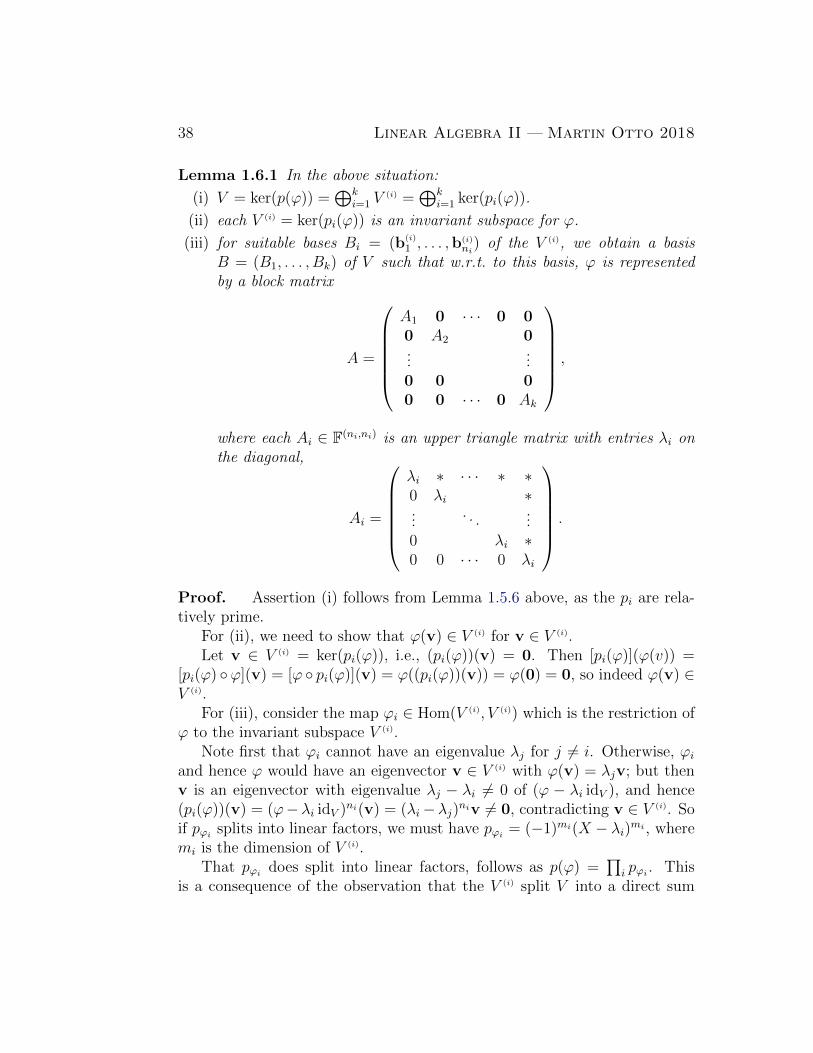
Lemma 1.6.1 In the above situation:
(i) V = ker(p(ϕ)) =⊕k
i=1 V(i) =
⊕ki=1 ker(pi(ϕ)).
(ii) each V (i) = ker(pi(ϕ)) is an invariant subspace for ϕ.
(iii) for suitable bases Bi = (b(i)
1 , . . . ,b(i)ni
) of the V (i), we obtain a basisB = (B1, . . . , Bk) of V such that w.r.t. to this basis, ϕ is representedby a block matrix
A =
A1 0 · · · 0 00 A2 0...
...0 0 00 0 · · · 0 Ak
,
where each Ai ∈ F(ni,ni) is an upper triangle matrix with entries λi onthe diagonal,
Ai =
λi ∗ · · · ∗ ∗0 λi ∗...
. . ....
0 λi ∗0 0 · · · 0 λi
.
Proof. Assertion (i) follows from Lemma 1.5.6 above, as the pi are rela-tively prime.
For (ii), we need to show that ϕ(v) ∈ V (i) for v ∈ V (i).Let v ∈ V (i) = ker(pi(ϕ)), i.e., (pi(ϕ))(v) = 0. Then [pi(ϕ)](ϕ(v)) =
[pi(ϕ) ◦ϕ](v) = [ϕ ◦ pi(ϕ)](v) = ϕ((pi(ϕ))(v)) = ϕ(0) = 0, so indeed ϕ(v) ∈V (i).
For (iii), consider the map ϕi ∈ Hom(V (i), V (i)) which is the restriction ofϕ to the invariant subspace V (i).
Note first that ϕi cannot have an eigenvalue λj for j 6= i. Otherwise, ϕiand hence ϕ would have an eigenvector v ∈ V (i) with ϕ(v) = λjv; but thenv is an eigenvector with eigenvalue λj − λi 6= 0 of (ϕ − λi idV ), and hence(pi(ϕ))(v) = (ϕ−λi idV )ni(v) = (λi−λj)niv 6= 0, contradicting v ∈ V (i). Soif pϕi splits into linear factors, we must have pϕi = (−1)mi(X − λi)mi , wheremi is the dimension of V (i).
That pϕi does split into linear factors, follows as p(ϕ) =∏
i pϕi . Thisis a consequence of the observation that the V (i) split V into a direct sum
LA II — Martin Otto 2018 39
of invariant subspaces, see (i) and (ii). Therefore, for any choice of basesBi for V (i), with corresponding representations Ai for ϕi, ϕ is representedw.r.t. the combined basis B = (B1, . . . , Bk) by a block diagonal matrix ofthe form of A in (iii) (see Lemma 1.1.12 above; but here we do not knowanything about the Ai yet). This implies that p = pϕ = pA = |A−XEn| =∏
i |Ai − XEmi | =∏
i pϕi , whence also the pϕi split into linear factors. Itthen follows that mi = ni = dim(V (i)).
Let finally then the basis Bi of V (i) be chosen according to Proposi-tion 1.3.1. This gives the desired form for the Ai.
2
Corollary 1.6.2 If pϕ = (−1)n∏k
i=1(X−λi)ni for pairwise distinct λi, thenV (i) = ker
((ϕ − λi idV )ni
)is an invariant subspace of dimension ni, and V
is the direct sum of these V (i).
1.6.2 Block decomposition, part 2
We turn to what emerged as the situation for ϕi above, i.e., for ϕ in restrictionto one of the invariant subspaces V (i).
We therefore now assume that p = pϕ = (−1)n(X−λ)n has a single linearfactor corresponding to the eigenvalue λ, of multiplicity n = dim(V ).
Note that the minimal polynomial qϕ must be of form qϕ = (X − λ)m forsome 1 6 m 6 n. We know that ϕ is diagonalisable iff m = 1. So, whathappens if m > 1? We study the situation with the help of the endomorphism
ψ = ϕ− λ idV .
Clearly pϕ(ϕ) = (−1)nψn and hence V = ker(ψn) by the Cayley–HamiltonTheorem. Moreover, the degree m of the minimal polynomial qϕ is the min-imal number m such that V = ker(ψm).
We therefore consider the subspaces
Uj := ker(ψj) ⊆ V for j = 0, . . . , n.
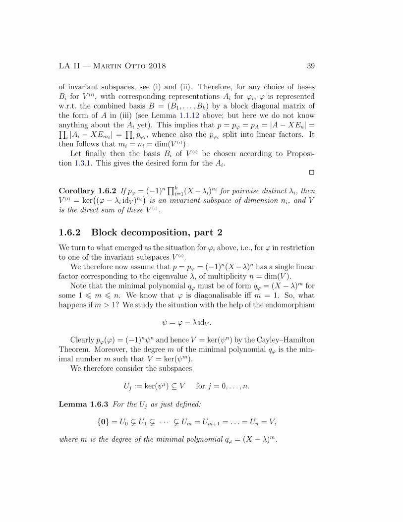
Lemma 1.6.3 For the Uj as just defined:
{0} = U0 U1 · · · Um = Um+1 = . . . = Un = V,
where m is the degree of the minimal polynomial qϕ = (X − λ)m.
40 Linear Algebra II — Martin Otto 2018
Um = V
Um−1
U2
U1 = Vλ
...
Proof. U0 = {0} as ψ0 = idV .U0 U1 as U1 = ker(ψ) = ker(ϕ− λ idV ) = Vλ is a non-trivial eigenspace
because λ is an eigenvalue of ϕ.Clearly Uj ⊆ Uj+1 for all j. Further, Uj = Uj+1 ⇒ Uj+1 = Uj+2, and
hence the sequence of the Uj becomes constant as soon as it does not strictlyincrease once. This is because
v ∈ Uj+2 \ Uj+1 iff ψ(v) ∈ Uj+1 \ Uj.
In particular, for the smallest m with Um = Um+1 it follows that alsoUm = V . It remains to argue that this smallest m is the degree of qϕ. Bythe definition of the minimal polynomial qϕ, ker(qϕ(ϕ)) = V and qϕ|q for anyother q such that ker(q(ϕ)) = V . Hence, as qϕ = ψ` for some `, the firstcondition tells us that ` > m, while the second implies that ` 6 m.
2
We can think now of V as stratified w.r.t. the chain of subspaces Uj.With a vector v ∈ V we associate its height h(v) w.r.t. this stratificationaccording to
h(v) := j iff v ∈ Uj \ Uj−1.The range of these heights is between 0 (v = 0 only) and the degree m
of qϕ. Note that for h(v) > 1:
h(ψ(v)) = h(v)− 1.
We first look at a vector v of height ` > 0, and at its iterated ψ-images,ψ(v), ψ(ψ(v)),. . . , which create a sequence of vectors of decreasing heights`, `− 1, . . . , 0.
LA II — Martin Otto 2018 41
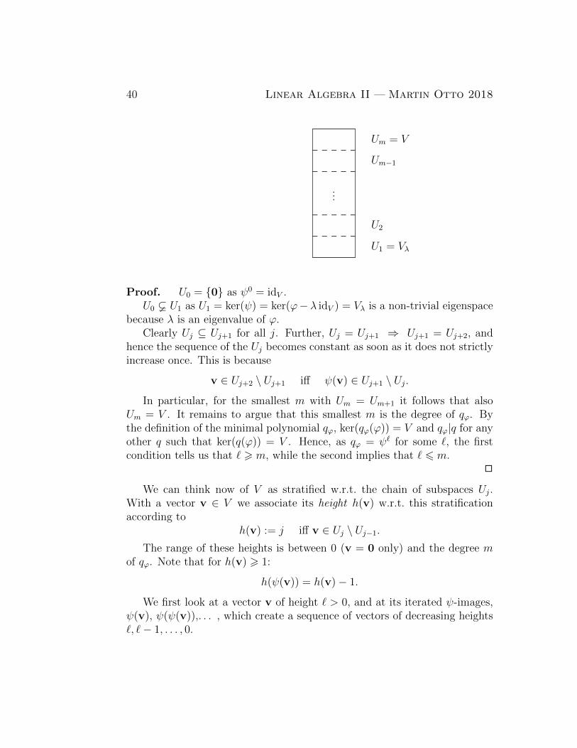
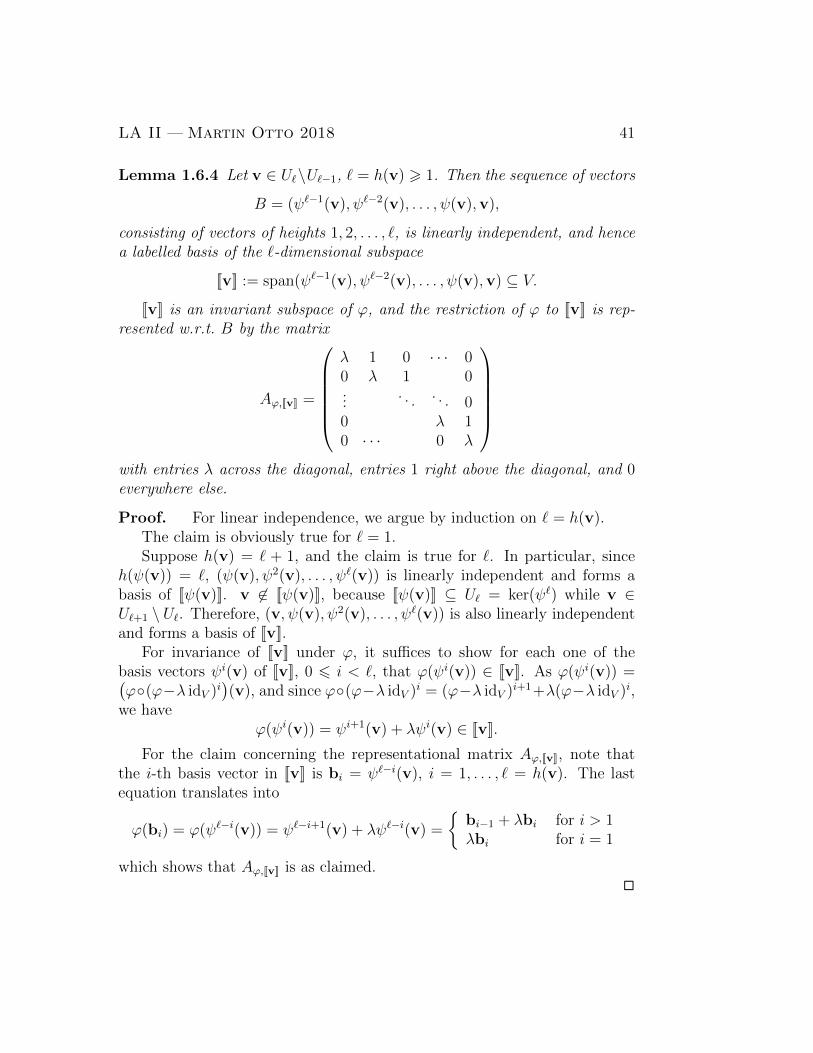
Lemma 1.6.4 Let v ∈ U`\U`−1, ` = h(v) > 1. Then the sequence of vectors
B = (ψ`−1(v), ψ`−2(v), . . . , ψ(v),v),
consisting of vectors of heights 1, 2, . . . , `, is linearly independent, and hencea labelled basis of the `-dimensional subspace
[[v]] := span(ψ`−1(v), ψ`−2(v), . . . , ψ(v),v) ⊆ V.
[[v]] is an invariant subspace of ϕ, and the restriction of ϕ to [[v]] is rep-resented w.r.t. B by the matrix
Aϕ,[[v]] =
λ 1 0 · · · 00 λ 1 0...
. . . . . . 00 λ 10 · · · 0 λ
with entries λ across the diagonal, entries 1 right above the diagonal, and 0everywhere else.
Proof. For linear independence, we argue by induction on ` = h(v).The claim is obviously true for ` = 1.Suppose h(v) = ` + 1, and the claim is true for `. In particular, since
h(ψ(v)) = `, (ψ(v), ψ2(v), . . . , ψ`(v)) is linearly independent and forms abasis of [[ψ(v)]]. v 6∈ [[ψ(v)]], because [[ψ(v)]] ⊆ U` = ker(ψ`) while v ∈U`+1 \ U`. Therefore, (v, ψ(v), ψ2(v), . . . , ψ`(v)) is also linearly independentand forms a basis of [[v]].
For invariance of [[v]] under ϕ, it suffices to show for each one of thebasis vectors ψi(v) of [[v]], 0 6 i < `, that ϕ(ψi(v)) ∈ [[v]]. As ϕ(ψi(v)) =(ϕ◦(ϕ−λ idV )i
)(v), and since ϕ◦(ϕ−λ idV )i = (ϕ−λ idV )i+1+λ(ϕ−λ idV )i,
we haveϕ(ψi(v)) = ψi+1(v) + λψi(v) ∈ [[v]].
For the claim concerning the representational matrix Aϕ,[[v]], note thatthe i-th basis vector in [[v]] is bi = ψ`−i(v), i = 1, . . . , ` = h(v). The lastequation translates into
ϕ(bi) = ϕ(ψ`−i(v)) = ψ`−i+1(v) + λψ`−i(v) =
{bi−1 + λbi for i > 1λbi for i = 1
which shows that Aϕ,[[v]] is as claimed.2
42 Linear Algebra II — Martin Otto 2018
Um
Um−1
Um−2
U1 = Vλ
•v
•ψ(v)
•ψ2(v)
•ψh(v)−1(v)
◦
◦
◦
◦
◦
◦
◦
��
��
��
��
��
��
��
��
��
��
��
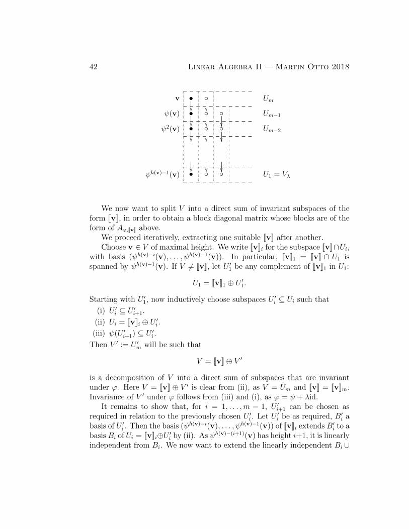
We now want to split V into a direct sum of invariant subspaces of theform [[v]], in order to obtain a block diagonal matrix whose blocks are of theform of Aϕ,[[v]] above.
We proceed iteratively, extracting one suitable [[v]] after another.Choose v ∈ V of maximal height. We write [[v]]i for the subspace [[v]]∩Ui,
with basis (ψh(v)−i(v), . . . , ψh(v)−1(v)). In particular, [[v]]1 = [[v]] ∩ U1 isspanned by ψh(v)−1(v). If V 6= [[v]], let U ′1 be any complement of [[v]]1 in U1:
U1 = [[v]]1 ⊕ U ′1.
Starting with U ′1, now inductively choose subspaces U ′i ⊆ Ui such that
(i) U ′i ⊆ U ′i+1.
(ii) Ui = [[v]]i ⊕ U ′i .(iii) ψ(U ′i+1) ⊆ U ′i .
Then V ′ := U ′m will be such that
V = [[v]]⊕ V ′
is a decomposition of V into a direct sum of subspaces that are invariantunder ϕ. Here V = [[v]] ⊕ V ′ is clear from (ii), as V = Um and [[v]] = [[v]]m.Invariance of V ′ under ϕ follows from (iii) and (i), as ϕ = ψ + λid.
It remains to show that, for i = 1, . . . ,m − 1, U ′i+1 can be chosen asrequired in relation to the previously chosen U ′i . Let U ′i be as required, B′i abasis of U ′i . Then the basis (ψh(v)−i(v), . . . , ψh(v)−1(v)) of [[v]]i extends B′i to abasisBi of Ui = [[v]]i⊕U ′i by (ii). As ψh(v)−(i+1)(v) has height i+1, it is linearlyindependent from Bi. We now want to extend the linearly independent Bi ∪
LA II — Martin Otto 2018 43
{ψh(v)−(i+1)(v)} to a basis Bi+1 of Ui+1 using new basis vectors b for whichψ(b) ∈ U ′i . Then B′i+1 := Bi+1 \ {ψh(v)−(i+1)(v), ψh(v)−i(v), . . . , ψh(v)−1(v)}can serve as a basis for the desired U ′i+1. Such an extension is possible dueto the following claim.
Claim 1.6.5 Ui+1 ⊆ [[v]]i+1 + {w ∈ Ui+1 : ψ(w) ∈ U ′i}.
Proof. Consider w ∈ Ui+1 \ Ui. Since h(w) = i + 1, h(ψ(w)) = i and,by (ii) for U ′i , ψ(w) = v′ + u′ for suitable v′ ∈ [[v]]i and u′ ∈ U ′i . Letv′ =
∑16j6i λjψ
h(v)−j(v). Putting v′′ :=∑
16j6i λjψh(v)−j−1(v), we have
v′′ ∈ [[v]]i+1 and ψ(v′′) = v′. Now w = v′′ + (w − v′′) and ψ(w − v′′) =ψ(w) − ψ(v′′) = ψ(w) − v′ = u′ ∈ U ′i shows that w ∈ [[v]]i+1 + {w ∈Ui+1 : ψ(w) ∈ U ′i}.
2
The process of eliminating one [[v]] (of maximal remaining height in V ′)after the other can be iterated as long as there remains a non-trivial comple-ment V ′. We thus obtain the following.
Lemma 1.6.6 If pϕ = (−1)n(X − λ)n and qϕ = (X − λ)m, then V canbe decomposed into a direct sum of invariant subspaces of the form [[v]] =span(v, ψ(v), . . . , ψh(v)−1(v)) for suitable v, such that the dimensions of thesesubspaces are m = `1 > · · · > `s > 1, with
∑j `j = n. Here s is the
dimension of the eigenspace Vλ.W.r.t. a basis obtained from the bases (ψh(v)−1(v), . . . ,v) of these sub-
spaces [[v]], as described in Lemma 1.6.4, ϕ is represented by a block diagonalmatrix with blocks of the form Aϕ,[[v]] described there.
Proof. Suitable [[v]] are successively obtained according to the above.Note that the first v, of maximal height m in V , gives rise to an invariantsubspace [[v]] of dimension m. All consecutive iterations of the process pro-duce contributions of weakly decreasing heights and dimensions, all greaterthan 0.
If V =⊕s
j=1[[vj]], then dim(V ) = n =∑
j dim([[vj]]). As any [[vj]] ∩U1 = [[vj]] ∩ Vλ has dimension 1, there are s = dim(Vλ) many successivecontributions; each involving (the span of) just one eigenvector ψh(vj)−1(vj).
The desired representation of ϕ follows with Lemma 1.1.12 (block de-composition in direct sums of invariant subspaces) and Lemma 1.6.4 (desiredshape for the blocks).
2
44 Linear Algebra II — Martin Otto 2018
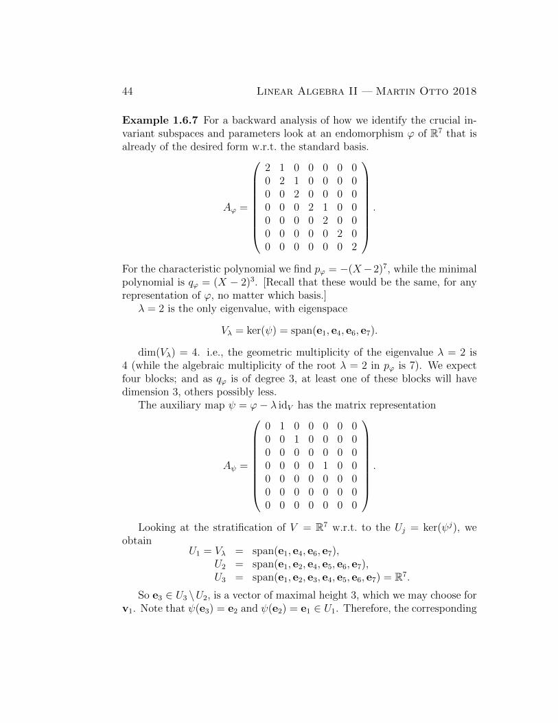
Example 1.6.7 For a backward analysis of how we identify the crucial in-variant subspaces and parameters look at an endomorphism ϕ of R7 that isalready of the desired form w.r.t. the standard basis.
Aϕ =
2 1 0 0 0 0 00 2 1 0 0 0 00 0 2 0 0 0 00 0 0 2 1 0 00 0 0 0 2 0 00 0 0 0 0 2 00 0 0 0 0 0 2
.
For the characteristic polynomial we find pϕ = −(X−2)7, while the minimalpolynomial is qϕ = (X − 2)3. [Recall that these would be the same, for anyrepresentation of ϕ, no matter which basis.]
λ = 2 is the only eigenvalue, with eigenspace
Vλ = ker(ψ) = span(e1, e4, e6, e7).
dim(Vλ) = 4. i.e., the geometric multiplicity of the eigenvalue λ = 2 is4 (while the algebraic multiplicity of the root λ = 2 in pϕ is 7). We expectfour blocks; and as qϕ is of degree 3, at least one of these blocks will havedimension 3, others possibly less.
The auxiliary map ψ = ϕ− λ idV has the matrix representation
Aψ =
0 1 0 0 0 0 00 0 1 0 0 0 00 0 0 0 0 0 00 0 0 0 1 0 00 0 0 0 0 0 00 0 0 0 0 0 00 0 0 0 0 0 0
.
Looking at the stratification of V = R7 w.r.t. to the Uj = ker(ψj), weobtain
U1 = Vλ = span(e1, e4, e6, e7),U2 = span(e1, e2, e4, e5, e6, e7),U3 = span(e1, e2, e3, e4, e5, e6, e7) = R7.
So e3 ∈ U3 \U2, is a vector of maximal height 3, which we may choose forv1. Note that ψ(e3) = e2 and ψ(e2) = e1 ∈ U1. Therefore, the corresponding
LA II — Martin Otto 2018 45
invariant subspace is [[e3]] = span(e1, e2, e3) — giving rise to the first block,
Aϕ,[[v1]] =
2 1 00 2 10 0 2
.
[[e3]] ∩ U1 = span(e1). As a complement for [[e3]] ∩ U1 we may chooseU ′1 = span(e4, e6, e7). The invariant subspace V ′ that is a complement of[[e3]] in V , is V ′ = span(e4, e5, e6, e7).
The restriction ϕ′ of ϕ to V ′ is represented w.r.t. the standard basis(e4, e5, e6, e7) for V ′, by
Aϕ′ =
2 1 0 00 2 0 00 0 2 00 0 0 2
.
Repeating the process for ϕ′ in V ′, one can choose v2 = e5 as a vector ofmaximal height in V ′; its height being 2: ψ(e5) = e4 ∈ U1. [One can checkthat pϕ′ = (X − 2)4 and qϕ′ = (X − 2)2.]
A corresponding invariant subspace is [[e5]] = span(e4, e5) — giving riseto the second block,
Aϕ,[[v2]] =
(2 10 2
).
A complement for [[v2]] ∩ U1 = span(e4) in U ′1 is U ′′1 = span(e6, e7). NowV ′′ = U ′′1 as there are no more vectors of height greater than 1. [The restric-tion ϕ′′ to V ′′ = span(e6, e7) has pϕ′′ = (X − 2)2 and qϕ′′ = (x− 2).] Henceϕ′′ is diagonal, and the remaining two blocks are both of of size 1.
1.6.3 Jordan normal form
Retracing our steps to the beginning, and combining the results for the firstand second block decompositions, we obtain the full statement of the Jordannormal form as follows.
Theorem 1.6.8 Let ϕ ∈ Hom(V, V ) such that pϕ splits into linear factors,
pϕ = (−1)nk∏i=1
(X − λi)ni .
46 Linear Algebra II — Martin Otto 2018
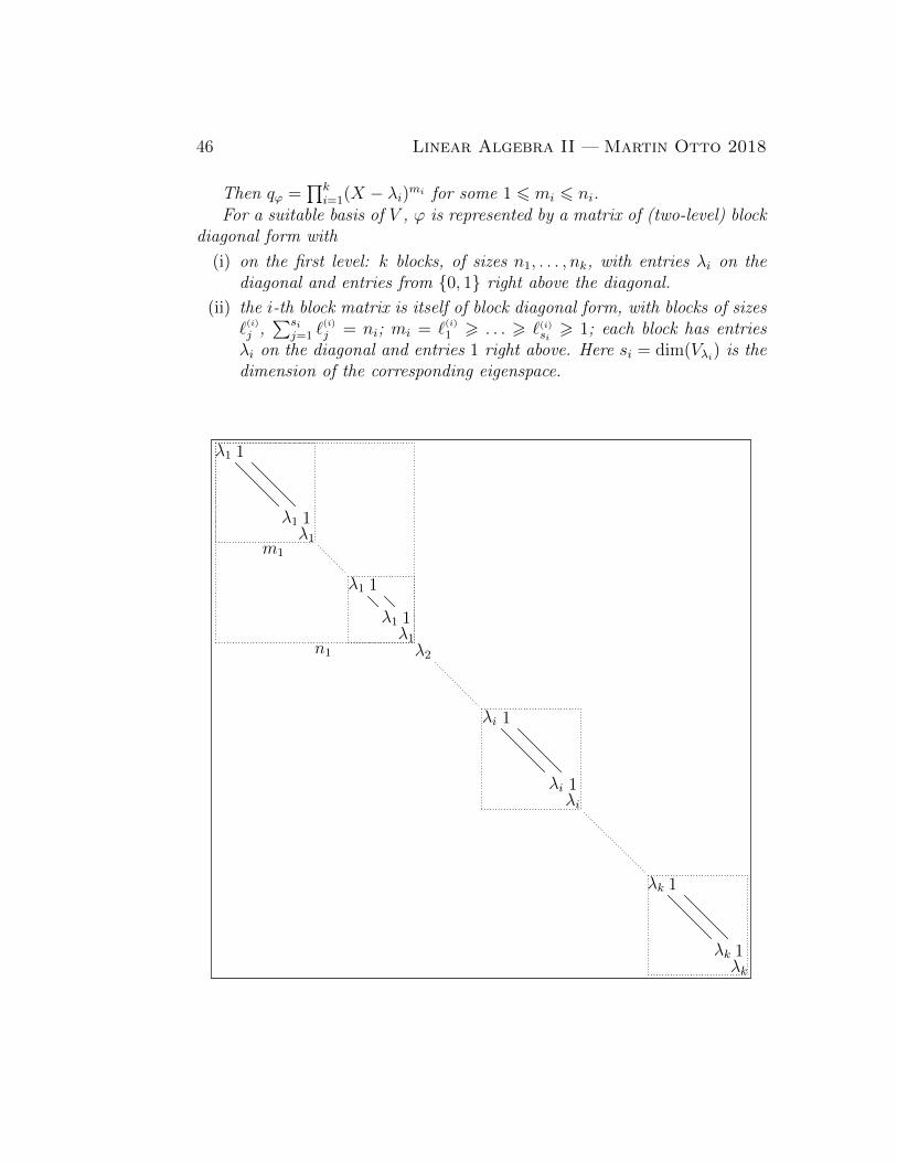
Then qϕ =∏k
i=1(X − λi)mi for some 1 6 mi 6 ni.For a suitable basis of V , ϕ is represented by a matrix of (two-level) block
diagonal form with
(i) on the first level: k blocks, of sizes n1, . . . , nk, with entries λi on thediagonal and entries from {0, 1} right above the diagonal.
(ii) the i-th block matrix is itself of block diagonal form, with blocks of sizes`(i)j ,
∑sij=1 `
(i)
j = ni; mi = `(i)1 > . . . > `(i)si > 1; each block has entriesλi on the diagonal and entries 1 right above. Here si = dim(Vλi) is thedimension of the corresponding eigenspace.
λ1
λ1λ1
m1
n1
1
1
λ1
λ1λ1
1
1
λ2
λk
λkλk
1
1
λi
λiλi
1
1
LA II — Martin Otto 2018 47
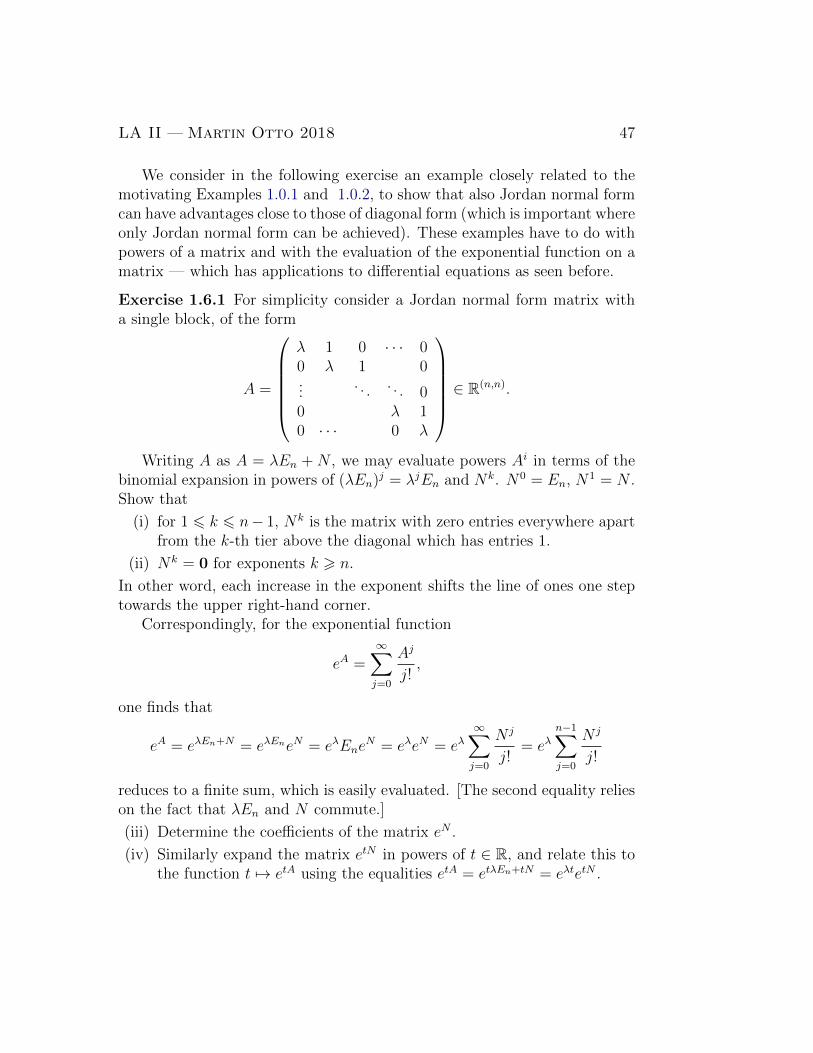
We consider in the following exercise an example closely related to themotivating Examples 1.0.1 and 1.0.2, to show that also Jordan normal formcan have advantages close to those of diagonal form (which is important whereonly Jordan normal form can be achieved). These examples have to do withpowers of a matrix and with the evaluation of the exponential function on amatrix — which has applications to differential equations as seen before.
Exercise 1.6.1 For simplicity consider a Jordan normal form matrix witha single block, of the form
A =
λ 1 0 · · · 00 λ 1 0...
. . . . . . 00 λ 10 · · · 0 λ
∈ R(n,n).
Writing A as A = λEn + N , we may evaluate powers Ai in terms of thebinomial expansion in powers of (λEn)j = λjEn and Nk. N0 = En, N1 = N .Show that
(i) for 1 6 k 6 n− 1, Nk is the matrix with zero entries everywhere apartfrom the k-th tier above the diagonal which has entries 1.
(ii) Nk = 0 for exponents k > n.
In other word, each increase in the exponent shifts the line of ones one steptowards the upper right-hand corner.
Correspondingly, for the exponential function
eA =∞∑j=0
Aj
j!,
one finds that
eA = eλEn+N = eλEneN = eλEneN = eλeN = eλ
∞∑j=0
N j
j!= eλ
n−1∑j=0
N j
j!
reduces to a finite sum, which is easily evaluated. [The second equality relieson the fact that λEn and N commute.]
(iii) Determine the coefficients of the matrix eN .
(iv) Similarly expand the matrix etN in powers of t ∈ R, and relate this tothe function t 7→ etA using the equalities etA = etλEn+tN = eλtetN .

48 Linear Algebra II — Martin Otto 2018
Chapter 2
Euclidean and Unitary Spaces
In this chapter we study vector spaces (over R and C) with additional metricstructure that allows us to speak of lengths [Lange, Betrag] of vectors andangles [Winkel] between vectors. The additional algebraic structure, over andabove the underlying vector space structure, is that of a (real or complex)scalar product [Skalarprodukt] that associates a scalar with every pair ofvectors.
It is clear that the vector space structure on its own does not support anygeometric notion of length: after all, re-scalings of the form ϕ : v 7→ λv, forarbitrary λ ∈ F\{0} are vector space automorphisms. Homomorphisms thatpreserve not just the vector space structure, but also the additional metricstructure, will correspondingly be length-preserving or isometric homomor-phisms, or isometries . We shall study these structure preserving maps inconnection with the structure of real and complex vectors spaces equippedwith a scalar product.
An R-vector space with a real-valued scalar product is called a euclideanspace, while a C-vector space with a C-valued scalar product is a uni-tary space. The main topics of this chapter are euclidean and unitary vec-tor spaces; corresponding bases with special metric properties (orthonormalbases); lengths, angles and orthogonality in such spaces; isometries of eu-clidean and unitary spaces; corresponding matrix groups; the representationsof vector space endomorphisms w.r.t. orthonormal bases; and diagonalisationof natural classes of homomorphisms and matrices that have special proper-ties in relation to the given scalar product.
49
50 Linear Algebra II — Martin Otto 2018
Column vectors and row vectors We now have occasion to fix a con-vention with regard to row and column vectors. We make the following stip-ulation for this whole chapter: all vectors in the standard spaces Fn (here:F = R or F = C) are written as column vectors. In other words, we identifyv ∈ Fn with an element of F(n,1) (slim matrices: n rows, one column). Therow vector corresponding to v is explicitly obtained as the transpose of v:
v =
v1...vn
∈ Fn = F(n,1) versus vt = (v1, . . . , vn) ∈ F(1,n).
Correspondingly, w.r.t. to some basis B = (b1, . . . ,bn) of the n-dimensionalF-vector space V , we think of the coefficients of a vector v =
∑ni=1 λibi as
forming the column vector
[[v]]B =
λ1...λn
∈ F(n,1) and write [[v]]tB for (λ1, . . . , λn).
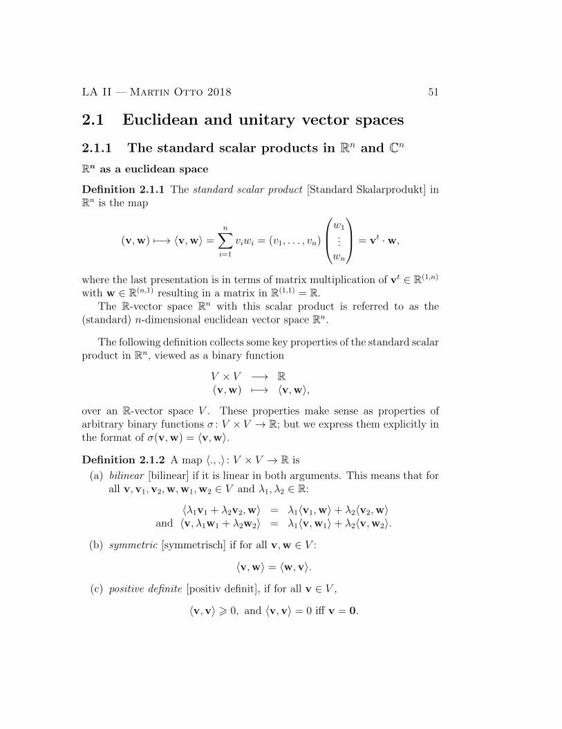
LA II — Martin Otto 2018 51
2.1 Euclidean and unitary vector spaces
2.1.1 The standard scalar products in Rn and Cn
Rn as a euclidean space
Definition 2.1.1 The standard scalar product [Standard Skalarprodukt] inRn is the map
(v,w) 7−→ 〈v,w〉 =n∑i=1
viwi = (v1, . . . , vn)
w1...wn
= vt ·w,
where the last presentation is in terms of matrix multiplication of vt ∈ R(1,n)
with w ∈ R(n,1) resulting in a matrix in R(1,1) = R.The R-vector space Rn with this scalar product is referred to as the
(standard) n-dimensional euclidean vector space Rn.
The following definition collects some key properties of the standard scalarproduct in Rn, viewed as a binary function
V × V −→ R(v,w) 7−→ 〈v,w〉,
over an R-vector space V . These properties make sense as properties ofarbitrary binary functions σ : V × V → R; but we express them explicitly inthe format of σ(v,w) = 〈v,w〉.
Definition 2.1.2 A map 〈., .〉 : V × V → R is
(a) bilinear [bilinear] if it is linear in both arguments. This means that forall v,v1,v2,w,w1,w2 ∈ V and λ1, λ2 ∈ R:
〈λ1v1 + λ2v2,w〉 = λ1〈v1,w〉+ λ2〈v2,w〉and 〈v, λ1w1 + λ2w2〉 = λ1〈v,w1〉+ λ2〈v,w2〉.
(b) symmetric [symmetrisch] if for all v,w ∈ V :
〈v,w〉 = 〈w,v〉.
(c) positive definite [positiv definit], if for all v ∈ V ,
〈v,v〉 > 0, and 〈v,v〉 = 0 iff v = 0.
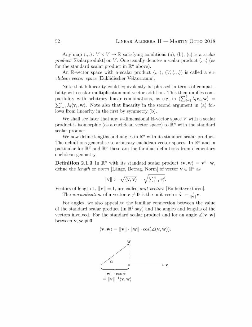
52 Linear Algebra II — Martin Otto 2018
Any map 〈., .〉 : V × V → R satisfying conditions (a), (b), (c) is a scalarproduct [Skalarprodukt] on V . One usually denotes a scalar product 〈., .〉 (asfor the standard scalar product in Rn above).
An R-vector space with a scalar product 〈., .〉, (V, 〈., .〉) is called a eu-clidean vector space [Euklidischer Vektorraum].
Note that bilinearity could equivalently be phrased in terms of compati-bility with scalar multiplication and vector addition. This then implies com-patibility with arbitrary linear combinations, as e.g. in 〈
∑ki=1 λivi,w〉 =∑k
i=1 λi〈vi,w〉. Note also that linearity in the second argument in (a) fol-lows from linearity in the first by symmetry (b).
We shall see later that any n-dimensional R-vector space V with a scalarproduct is isomorphic (as a euclidean vector space) to Rn with the standardscalar product.
We now define lengths and angles in Rn with its standard scalar product.The definitions generalise to arbitrary euclidean vector spaces. In Rn and inparticular for R2 and R3 these are the familiar definitions from elementaryeuclidean geometry.
Definition 2.1.3 In Rn with its standard scalar product 〈v,w〉 = vt · w,define the length or norm [Lange, Betrag, Norm] of vector v ∈ Rn as
‖v‖ :=√〈v,v〉 =
√∑ni=1 v
2i .
Vectors of length 1, ‖v‖ = 1, are called unit vectors [Einheitsvektoren].The normalisation of a vector v 6= 0 is the unit vector v := 1
‖v‖v.
For angles, we also appeal to the familiar connection between the valueof the standard scalar product (in R2 say) and the angles and lengths of thevectors involved. For the standard scalar product and for an angle ](v,w)between v,w 6= 0:
〈v,w〉 = ‖v‖ · ‖w‖ · cos(](v,w)).
◦ v
w
α︸ ︷︷ ︸‖w‖ · cosα
= ‖v‖−1〈v,w〉
//
;;
LA II — Martin Otto 2018 53
Definition 2.1.4 The (pointed) angle between vectors v,w ∈ Rn \ {0} isdefined by
](v,w) := arccos( 〈v,w〉‖v‖‖w‖
)∈ [0, π].
Two vectors v and w are said to be orthogonal [orthogonal], denotedv⊥w, if 〈v,w〉 = 0.
Clearly for v,w 6= 0, v⊥w iff ](v,w) = π/2.
2.1.2 Cn as a unitary space
For the complex analogue Cn, the standard scalar product also needs toreturn a non-negative real number for the induced norm ‖v‖ =
√〈v,v〉,
rather than an arbitrary complex number. Recall that the absolute value ofa complex number z = x+iy is |z| =
√x2 + y2 =
√zz. Complex conjugation
is used to the same effect in the following definition of the standard scalarproduct on Cn.
We adopt the notation u for the vector obtained from u ∈ Cn by compo-nent-wise complex conjugation:
u =
u1...un
∈ Cn 7−→ u =
u1...un
∈ Cn.Note that the map u 7→ u is not linear over Cn. While it is compatible
with vector addition in Cn, it is not compatible with scalar multiplication:instead of C-linear w.r.t. scalars it is conjugated-linear, mapping λu to λurather than to λu.
We shall also often need the row vector corresponding to u, which isthe transpose ut. For the combined operation of (component-wise) complexconjugation and transposition we use the standard notation
u =
u1...un
7−→ u+ := ut = (u1, . . . , un),
which really is a special case of the adjoint operation (on matrices) to bedefined in Definition 2.1.8 below.
54 Linear Algebra II — Martin Otto 2018
Definition 2.1.5 The standard scalar product 1 in Cn is the map
(v,w) 7−→ 〈v,w〉 =n∑i=1
viwi = (v1, . . . , vn)
w1...wn
= vt ·w = v+w.
The C-vector space Cn with this scalar product is referred to as the(standard) n-dimensional unitary vector space Cn.
Again we collect properties of this standard scalar product, viewed as abinary function
V × V −→ C(v,w) 7−→ 〈v,w〉,
which could also be phrased for any binary function σ : V × V → C.
Definition 2.1.6 A map 〈., .〉 : V × V → C is
(a) semi-bilinear (also: sesquilinear) [semi-bilinear, sesquilinear] if for allv,v1,v2,w,w1,w2 ∈ V and λ1, λ2 ∈ C
(i) (linear in its second argument)
〈v, λ1w1 + λ2w2〉 = λ1〈v,w1〉+ λ2〈v,w2〉.
(ii) (conjugated-linear in the first argument)
〈λ1v1 + λ2v2,w〉 = λ1〈v1,w〉+ λ2〈v2,w〉.
(b) hermitian [hermitesch], if for all v,w ∈ V
〈v,w〉 = 〈w,v〉.
(c) positive definite [positiv definit], if for all v ∈ V
〈v,v〉 > 0 in R, and 〈v,v〉 = 0 iff v = 0.
Any σ satisfying conditions (a), (b), (c) is a (complex) scalar product onV , usually denoted 〈., .〉.
A C-vector space V with a scalar product 〈., .〉, (V, 〈., .〉), is called aunitary vector space [unitarer Vektorraum].
1Beware that there are two conventions in the literature, as to whether a complex scalarproduct is linear in its first or in its second argument. We here follow the convention oflinearity in the second argument.
LA II — Martin Otto 2018 55
Note that 〈v,v〉 ∈ R follows from (b), as we have for all z ∈ C that z ∈ Riff z = z. Also, (ii) in (a) follows from (i) together with (b).
Lengths and orthogonality in Cn are defined w.r.t. the standard scalarproduct in complete analogy with Rn.
Definition 2.1.7 In Cn with its standard scalar product 〈v,w〉 = v+w, thelength or norm of vector v ∈ Cn is
‖v‖ :=√〈v,v〉 =
√∑ni=1 vivi =
√∑ni=1 |vi|2.
Vectors of length 1, ‖v‖ = 1, are called unit vectors [Einheitsvektoren].Vectors v,w ∈ Cn are called orthogonal iff 〈v,w〉 = 0.
2.1.3 Bilinear and semi-bilinear forms
Before further exploration of scalar products in R- and C-vector spaces, webriefly consider bilinear and semi-bilinear forms in general and in particularlink them to matrices for their representation w.r.t. to chosen bases. Keepin mind that scalar products are special bilinear/semi-bilinear forms.
Bilinear forms in R-vector spaces
Let V be an n-dimensional R-vector space. Recall that a map σ : V ×V → Ris called a bilinear form [Bilinearform] if it is linear in each argument.
With respect to a basis B = (b1, . . . ,bn) of V , a bilinear form σ on V isuniquely determined by the values
aij := σ(bi,bj) ∈ R,
since, by bilinearity, for v =∑
i λibi and w =∑
i µibi, we get
σ(v,w) = σ(∑
i λibi,∑
i µibi) =∑i,j
λiµjσ(bi,bj) =∑i,j
λiµjaij.
Associate with σ the matrix A = [[σ]]B = (aij) ∈ R(n,n) as its representa-tion with respect to basis B,
[[σ]]B := (aij) ∈ R(n,n) where aij = σ(bi,bj).
56 Linear Algebra II — Martin Otto 2018
Then, in terms of coefficients w.r.t. basis B, and for vectors v =∑
i λibiand w =
∑i µibi:
σ(v,w) =∑
i,j λiµjaij = (λ1, . . . , λn)
a11 · · · a1n...
...an1 . . . ann
µ1
...µn
= [[v]]tB [[σ]]B [[w]]B.
Application of σ corresponds to a matrix product that multiplies the rowand column vectors corresponding to v and w, respectively, from the left andright into matrix A = [[σ]]B.
The matrix that represents the standard scalar product w.r.t. to the stan-dard basis of Rn, is just the unit matrix En.
Exercise 2.1.1 Show that a bilinear form σ on V is symmetric, i.e., thatσ(v,w) = σ(w,v) for all v,w ∈ V , iff the matrix A = [[σ]]B that representsσ w.r.t. some (any) basis B is symmetric in the sense that A = At.
A usefull alternative view of the representation
σ(v,w) = [[v]]tB[[σ]]B[[w]]B =∑i,j
λiµjaij = (λ1, . . . , λn) A
µ1...µn
,
where A[[σ]]B = (aij) = (σ(bi,bj)) is the following. Regard the column vectorA(µ1, . . . , µn)t as the representation of the image of w under the linear mapϕ for which [[ϕ]]BB = A:
w 7−→ ϕ(w) w.r.t. basis B: [[w]]B =
µ1...µn
7−→ [[ϕ(w)]]B = A
µ1...µn
.
In these terms, σ(v,w) is the standard scalar product of [[v]]B and [[ϕ(w)]]B:
σ(v,w) = (λ1, . . . , λn) A
µ1...µn
= 〈[[v]]B, [[ϕ(w)]]B〉 = [[v]]tB[[ϕ]]BB[[w]]B.
LA II — Martin Otto 2018 57
Semi-bilinear forms in a C-vector space
Let V be an n-dimensional C-vector space, σ : V × V → C a semi-bilinearform (cf. Definition 2.1.6 (a)). With respect to a basis B = (b1, . . . ,bn)of a C-vector space V , a semi-bilinear form σ is represented by the matrixA = [[σ]]B ∈ C(n,n) whose entries are
aij := σ(bi,bj) ∈ C.
By semi-bilinearity, for v =∑
i λibi and w =∑
i µibi, we get
σ(v,w) = σ(∑
i λibi,∑
i µibi) =∑
i,j λiµjσ(bi,bj) =∑
i,j λiµjaij
= (λ1, . . . , λn)
a11 · · · a1n...
...an1 . . . ann
µ1
...µn
= (λ1, . . . , λn) A
µ1...µn
= [[v]]+B[[σ]]B[[w]]B.
So, application of σ corresponds to a matrix product that multiplies therow and column vectors corresponding to the complex conjugate of v and w,respectively, from the left and right into matrix A = [[σ]]B. Again, the unitmatrix represents the standard scalar product (w.r.t. any basis).
Definition 2.1.8 For a matrix A ∈ C(n,n) its adjoint matrix [Adjungierte]is defined as the matrix A+ = (A)t = At, the result of taking the complexconjugate of all entries and applying transposition. For A = (aij), the entriesa+ij of A+ are a+ij = aji.
A matrix A ∈ C(n,n) is called hermitian or self-adjoint [hermitisch, selbst-adjungiert] iff A = A+.
Exercise 2.1.2 Show that a semi-bilinear form σ on V is hermitian iff thematrix A = [[σ]]B that represents σ w.r.t. some (any) basis B is hermitian.
Observation 2.1.9 The following rules apply w.r.t. the operations of com-plex conjugation and transposition of matrices in C(n,n):
(i) A+B = A+B and AB = AB.
(ii) (A+B)t = At +Bt and (AB)t = BtAt (order inverted!).
(iii) (A+B)+ = A+ +B+ and (AB)+ = B+A+ (order inverted!).
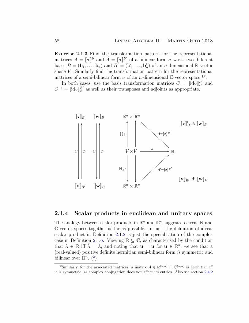
58 Linear Algebra II — Martin Otto 2018
Exercise 2.1.3 Find the transformation pattern for the representationalmatrices A = [[σ]]B and A = [[σ]]B
′of a bilinear form σ w.r.t. two different
bases B = (b1, . . . ,bn) and B′ = (b′1, . . . ,b′n) of an n-dimensional R-vector
space V . Similarly find the transformation pattern for the representationalmatrices of a semi-bilinear form σ of an n-dimensional C-vector space V .
In both cases, use the basis transformation matrices C = [[idV ]]BB′ andC−1 = [[idV ]]B
′B as well as their transposes and adjoints as appropriate.
[[v]]B [[w]]B
[[v]]B′ [[w]]B
Rn × Rn
Rn × Rn
V ×V R
[[v]]tB A [[w]]B
[[v]]tB′ A′ [[w]]B′
C
��
C′
OO
C
��
C′
OO
[[·]]B
OO OO
[[·]]B′
�� ��
σ //
A=[[σ]]B
A′=[[σ]]B′
>>
2.1.4 Scalar products in euclidean and unitary spaces
The analogy between scalar products in Rn and Cn suggests to treat R andC-vector spaces together as far as possible. In fact, the definition of a realscalar product in Definition 2.1.2 is just the specialisation of the complexcase in Definition 2.1.6. Viewing R ⊆ C, as characterised by the conditionthat λ ∈ R iff λ = λ, and noting that u = u for u ∈ Rn, we see that a(real-valued) positive definite hermitian semi-bilinear form is symmetric andbilinear over Rn. (2)
2Similarly, for the associated matrices, a matrix A ∈ R(n,n) ⊆ C(n,n) is hermitian iffit is symmetric, as complex conjugation does not affect its entries. Also see section 2.4.2
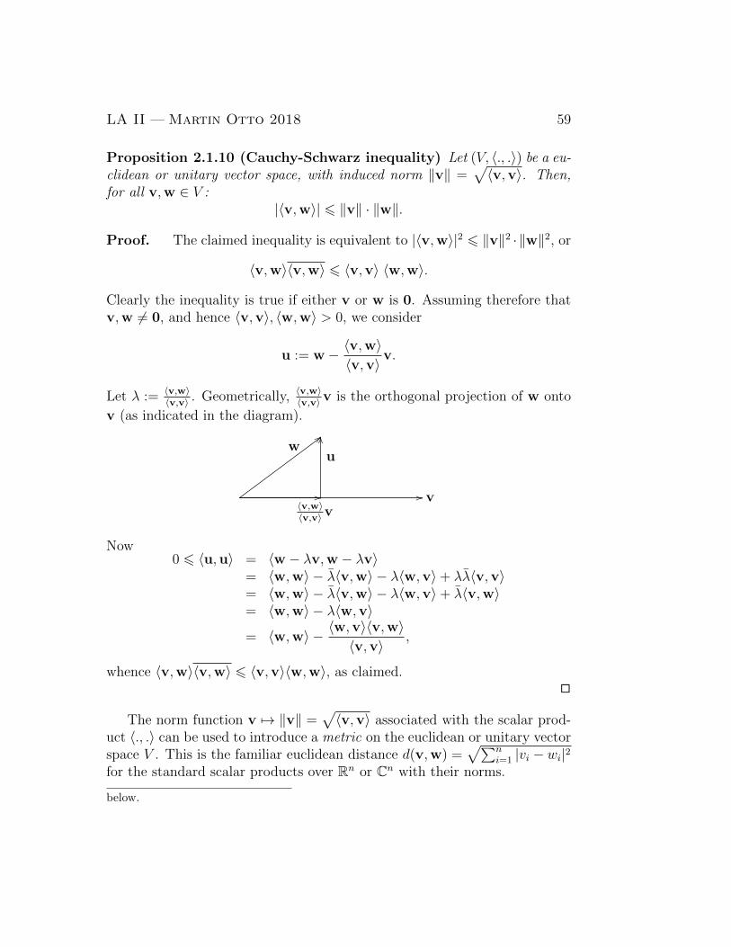
LA II — Martin Otto 2018 59
Proposition 2.1.10 (Cauchy-Schwarz inequality) Let (V, 〈., .〉) be a eu-clidean or unitary vector space, with induced norm ‖v‖ =
√〈v,v〉. Then,
for all v,w ∈ V :|〈v,w〉| 6 ‖v‖ · ‖w‖.
Proof. The claimed inequality is equivalent to |〈v,w〉|2 6 ‖v‖2 · ‖w‖2, or
〈v,w〉〈v,w〉 6 〈v,v〉 〈w,w〉.
Clearly the inequality is true if either v or w is 0. Assuming therefore thatv,w 6= 0, and hence 〈v,v〉, 〈w,w〉 > 0, we consider
u := w − 〈v,w〉〈v,v〉
v.
Let λ := 〈v,w〉〈v,v〉 . Geometrically, 〈v,w〉〈v,v〉 v is the orthogonal projection of w onto
v (as indicated in the diagram).
v
w
〈v,w〉〈v,v〉 v
u
OO
//
;;
//
Now0 6 〈u,u〉 = 〈w − λv,w − λv〉
= 〈w,w〉 − λ〈v,w〉 − λ〈w,v〉+ λλ〈v,v〉= 〈w,w〉 − λ〈v,w〉 − λ〈w,v〉+ λ〈v,w〉= 〈w,w〉 − λ〈w,v〉
= 〈w,w〉 − 〈w,v〉〈v,w〉〈v,v〉
,
whence 〈v,w〉〈v,w〉 6 〈v,v〉〈w,w〉, as claimed.2
The norm function v 7→ ‖v‖ =√〈v,v〉 associated with the scalar prod-
uct 〈., .〉 can be used to introduce a metric on the euclidean or unitary vectorspace V . This is the familiar euclidean distance d(v,w) =
√∑ni=1 |vi − wi|2
for the standard scalar products over Rn or Cn with their norms.
below.
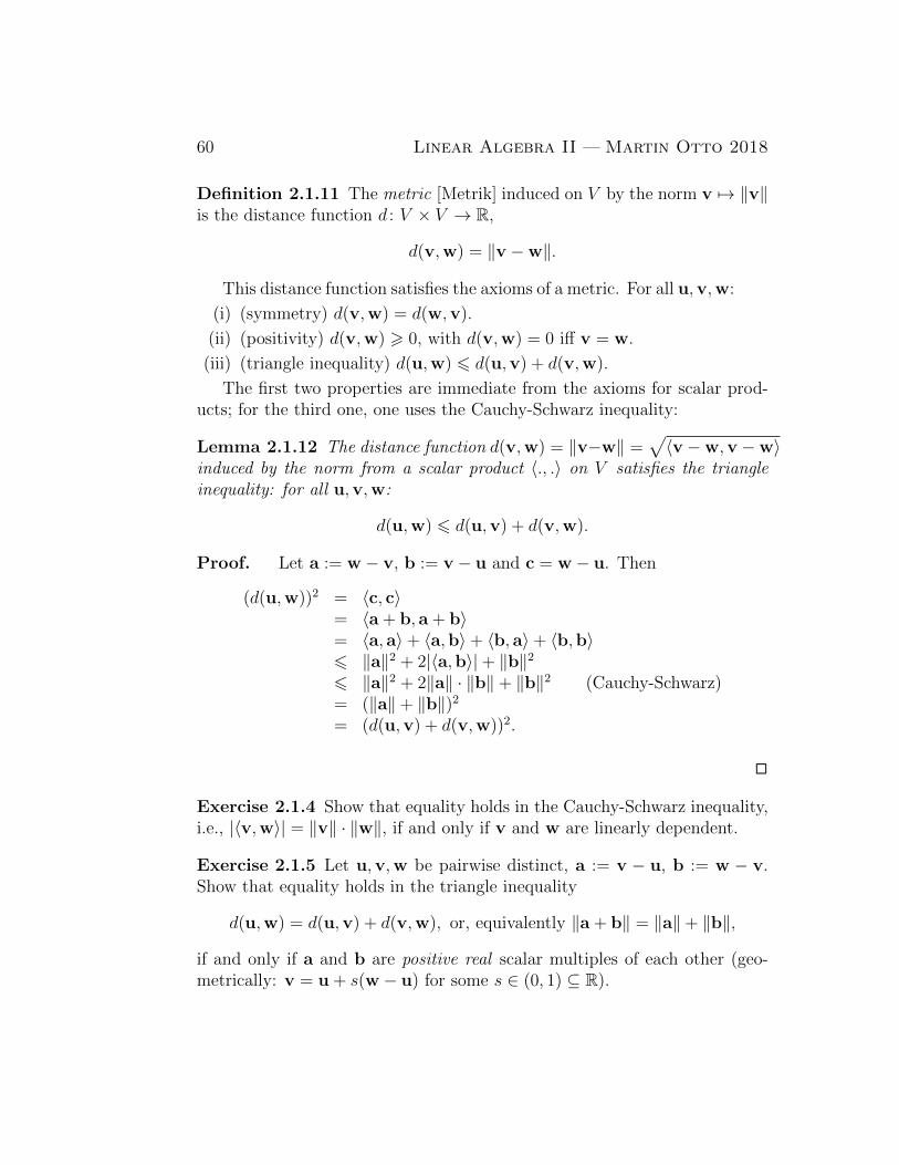
60 Linear Algebra II — Martin Otto 2018
Definition 2.1.11 The metric [Metrik] induced on V by the norm v 7→ ‖v‖is the distance function d : V × V → R,
d(v,w) = ‖v −w‖.
This distance function satisfies the axioms of a metric. For all u,v,w:
(i) (symmetry) d(v,w) = d(w,v).
(ii) (positivity) d(v,w) > 0, with d(v,w) = 0 iff v = w.
(iii) (triangle inequality) d(u,w) 6 d(u,v) + d(v,w).
The first two properties are immediate from the axioms for scalar prod-ucts; for the third one, one uses the Cauchy-Schwarz inequality:
Lemma 2.1.12 The distance function d(v,w) = ‖v−w‖ =√〈v −w,v −w〉
induced by the norm from a scalar product 〈., .〉 on V satisfies the triangleinequality: for all u,v,w:
d(u,w) 6 d(u,v) + d(v,w).
Proof. Let a := w − v, b := v − u and c = w − u. Then
(d(u,w))2 = 〈c, c〉= 〈a + b, a + b〉= 〈a, a〉+ 〈a,b〉+ 〈b, a〉+ 〈b,b〉6 ‖a‖2 + 2|〈a,b〉|+ ‖b‖26 ‖a‖2 + 2‖a‖ · ‖b‖+ ‖b‖2 (Cauchy-Schwarz)= (‖a‖+ ‖b‖)2= (d(u,v) + d(v,w))2.
2
Exercise 2.1.4 Show that equality holds in the Cauchy-Schwarz inequality,i.e., |〈v,w〉| = ‖v‖ · ‖w‖, if and only if v and w are linearly dependent.
Exercise 2.1.5 Let u,v,w be pairwise distinct, a := v − u, b := w − v.Show that equality holds in the triangle inequality
d(u,w) = d(u,v) + d(v,w), or, equivalently ‖a + b‖ = ‖a‖+ ‖b‖,
if and only if a and b are positive real scalar multiples of each other (geo-metrically: v = u + s(w − u) for some s ∈ (0, 1) ⊆ R).
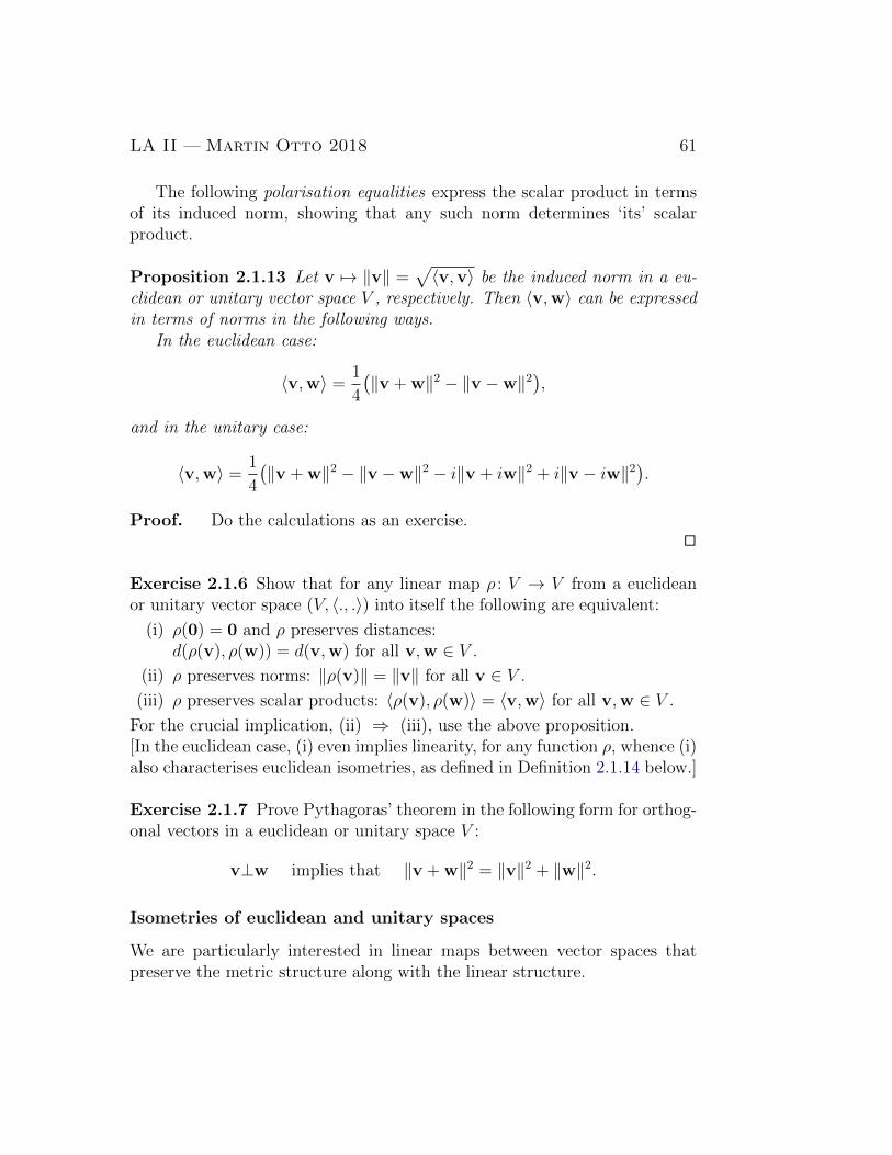
LA II — Martin Otto 2018 61
The following polarisation equalities express the scalar product in termsof its induced norm, showing that any such norm determines ‘its’ scalarproduct.
Proposition 2.1.13 Let v 7→ ‖v‖ =√〈v,v〉 be the induced norm in a eu-
clidean or unitary vector space V , respectively. Then 〈v,w〉 can be expressedin terms of norms in the following ways.
In the euclidean case:
〈v,w〉 =1
4
(‖v + w‖2 − ‖v −w‖2
),
and in the unitary case:
〈v,w〉 =1
4
(‖v + w‖2 − ‖v −w‖2 − i‖v + iw‖2 + i‖v − iw‖2
).
Proof. Do the calculations as an exercise.2
Exercise 2.1.6 Show that for any linear map ρ : V → V from a euclideanor unitary vector space (V, 〈., .〉) into itself the following are equivalent:
(i) ρ(0) = 0 and ρ preserves distances:d(ρ(v), ρ(w)) = d(v,w) for all v,w ∈ V .
(ii) ρ preserves norms: ‖ρ(v)‖ = ‖v‖ for all v ∈ V .
(iii) ρ preserves scalar products: 〈ρ(v), ρ(w)〉 = 〈v,w〉 for all v,w ∈ V .
For the crucial implication, (ii) ⇒ (iii), use the above proposition.[In the euclidean case, (i) even implies linearity, for any function ρ, whence (i)also characterises euclidean isometries, as defined in Definition 2.1.14 below.]
Exercise 2.1.7 Prove Pythagoras’ theorem in the following form for orthog-onal vectors in a euclidean or unitary space V :
v⊥w implies that ‖v + w‖2 = ‖v‖2 + ‖w‖2.
Isometries of euclidean and unitary spaces
We are particularly interested in linear maps between vector spaces thatpreserve the metric structure along with the linear structure.
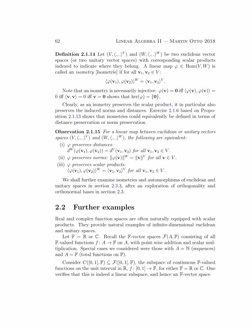
62 Linear Algebra II — Martin Otto 2018
Definition 2.1.14 Let (V, 〈., .〉V ) and (W, 〈., .〉W ) be two euclidean vectorspaces (or two unitary vector spaces) with corresponding scalar productsindexed to indicate where they belong. A linear map ϕ ∈ Hom(V,W ) iscalled an isometry [Isometrie] if for all v1,v2 ∈ V :
〈ϕ(v1), ϕ(v2)〉W = 〈v1,v2〉V .
Note that an isometry is necessarily injective: ϕ(v) = 0 iff 〈ϕ(v), ϕ(v)〉 =0 iff 〈v,v〉 = 0 iff v = 0 shows that ker(ϕ) = {0}.
Clearly, as an isometry preserves the scalar product, it in particular alsopreserves the induced norms and distances. Exercise 2.1.6 based on Propo-sition 2.1.13 shows that isometries could equivalently be defined in terms ofdistance preservation or norm preservation.
Observation 2.1.15 For a linear map between euclidean or unitary vectorsspaces (V, 〈., .〉V ) and (W, 〈., .〉W ), the following are equivalent:
(i) ϕ preserves distances:dW (ϕ(v1), ϕ(v2)) = dV (v1,v2) for all v1,v2 ∈ V .
(ii) ϕ preserves norms: ‖ϕ(v)‖W = ‖v‖V for all v ∈ V .
(iii) ϕ preserves scalar products:〈ϕ(v1), ϕ(v2)〉W = 〈v1,v2〉V for all v1,v2 ∈ V .
We shall further examine isometries and automorphisms of euclidean andunitary spaces in section 2.3.3, after an exploration of orthogonality andorthonormal bases in section 2.3.
2.2 Further examples
Real and complex function spaces are often naturally equipped with scalarproducts. They provide natural examples of infinite-dimensional euclideanand unitary spaces.
Let F = R or C. Recall the F-vector spaces F(A,F) consisting of allF-valued functions f : A→ F on A, with point-wise addition and scalar mul-tiplication. Special cases we considered were those with A = N (sequences)and A = F (total functions on F).
Consider C([0, 1],F) ⊆ F([0, 1],F), the subspace of continuous F-valuedfunctions on the unit interval in R, f : [0, 1]→ F, for either F = R or C. Oneverifies that this is indeed a linear subspace, and hence an F-vector space.
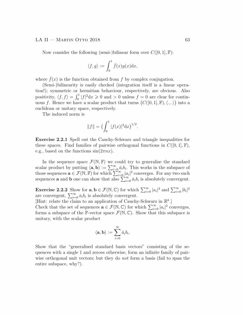
LA II — Martin Otto 2018 63
Now consider the following (semi-)bilinear form over C([0, 1],F):
〈f, g〉 :=
∫ 1
0
f(x)g(x)dx,
where f(x) is the function obtained from f by complex conjugation.(Semi-)bilinearity is easily checked (integration itself is a linear opera-
tion!); symmetric or hermitian behaviour, respectively, are obvious. Also
positivity, 〈f, f〉 =∫ 1
0|f |2dx > 0 and > 0 unless f = 0 are clear for contin-
uous f . Hence we have a scalar product that turns(C([0, 1],F), 〈., .〉
)into a
euclidean or unitary space, respectively.The induced norm is
‖f‖ =(∫ 1
0
|f(x)|2dx)1/2
.
Exercise 2.2.1 Spell out the Cauchy-Schwarz and triangle inequalities forthese spaces. Find families of pairwise orthogonal functions in C([0, 1],F),e.g., based on the functions sin(2πnx).
In the sequence space F(N,F) we could try to generalise the standardscalar product by putting 〈a,b〉 :=
∑∞i=0 aibi. This works in the subspace of
those sequences a ∈ F(N,F) for which∑∞
i=0 |ai|2 converges. For any two suchsequences a and b one can show that also
∑∞i=0 aibi is absolutely convergent.
Exercise 2.2.2 Show for a,b ∈ F(N,C) for which∑∞
i=0 |ai|2 and∑∞
i=0 |bi|2are convergent,
∑∞i=0 aibi is absolutely convergent.
[Hint: relate the claim to an application of Cauchy-Schwarz in Rk.]Check that the set of sequences a ∈ F(N,C) for which
∑∞i=0 |ai|2 converges,
forms a subspace of the F-vector space F(N,C). Show that this subspace isunitary, with the scalar product
〈a,b〉 :=∞∑i=0
aibi.
Show that the “generalised standard basis vectors” consisting of the se-quences with a single 1 and zeroes otherwise, form an infinite family of pair-wise orthogonal unit vectors; but they do not form a basis (fail to span theentire subspace, why?).
64 Linear Algebra II — Martin Otto 2018
2.3 Orthogonality and orthonormal bases
2.3.1 Orthonormal bases
Definition 2.3.1 A set (or family) S of vectors in a euclidean or unitaryvector space V is said to be an orthonormal system [Orthonormalsystem] ifit consist of pairwise orthogonal unit vectors: ‖u‖ = 1 for all u ∈ S andu⊥u′ for all u 6= u′ in S.
An orthonormal system that is a basis (of V or of some subspace U ⊆ V )is called an orthonormal basis [Orthonormalbasis].
Clearly the standard bases of Rn and Cn are orthonormal bases for thestandard scalar products.
The coefficients of vectors w.r.t. an orthonormal basis can be expressedin terms of the scalar product very easily.
Lemma 2.3.2 Let B = (b1, . . . ,bn) be an orthonormal basis of V . For allv ∈ V :
v =n∑i=1
〈bi,v〉bi, i.e., [[v]]B =
〈b1,v〉...
〈bn,v〉
.
Proof. Simply express v as a linear combination v =∑
i λibi and applyscalar products with bj to determine the coefficients λj:
〈bj,v〉 = 〈bj,∑i
λibi〉 =∑i
λi〈bj,bi〉 = λj.
2
Corollary 2.3.3 A basis B = (b1, . . . ,bn) of V is orthonormal iff the matrixrepresentation of the scalar product 〈., .〉 as a (semi-)bilinear form w.r.t. Bis the unit matrix: [[σ]]B = En for σ(v,w) := 〈v,w〉.
In other words: in terms of coefficients w.r.t. an orthonormal basis, thescalar product 〈., .〉 of V is computed just like the standard scalar productin the corresponding standard space Rn or Cn.
LA II — Martin Otto 2018 65
Gram-Schmidt orthonormalisation
The following is an existence theorem for orthonormal bases. We restrictattention to finite-dimensional euclidean or unitary vector spaces (V, 〈., .〉).The constructive proof provides a method to obtain an orthonormal basisfrom an arbitrary given basis.
Theorem 2.3.4 Let (V, 〈., .〉) be an n-dimensional euclidean or unitary vec-tor space with basis B = (b1, . . . ,bn).
Then there is an orthonormal basis B = (b1, . . . , bn) for V such that for1 6 k 6 n, span(b1, . . . ,bk) = span(b1, . . . , bk).
Proof. The proof is by the Gram-Schmidt procedure that successivelyconstructs the new basis vectors form the given ones. Formally we proceedby induction on k, constructing a sequence B1 ⊆ B1 ⊆ · · · ⊆ Bk such thatBk = (b1, . . . , bk) is an orthonormal basis of Uk := span(b1, . . . ,bk) ⊆ V .
Base case: k = 1. Let b1 := 1‖b1‖b1. Clearly B1 := {b1} is as desired.
In the induction step we assume that Bk = (b1, . . . , bk) is an orthonormalbasis of Uk and need to find a next unit vector bk+1 such that
(i) bk+1 ∈ Uk+1 = Uk + span(bk+1) = span(Bk) + span(bk+1).
(ii) ‖bk+1‖ = 1 and bk+1⊥ span(Bk), i.e., bk+1⊥ bi for i = 1, . . . , k.
Note that (i) and (ii) together imply that Bk+1 := (Bk, bk+1) spans Uk+1 andthat it is an orthonormal basis of this subspace.
Put
u :=k∑i=1
〈bi,bk+1〉bi.
Geometrically, u is the orthogonal projection of bk+1 onto Uk = span(Bk)(see section 2.3.2 below). Clearly u ∈ Uk and (bk+1 − u)⊥Uk, as for everybasis vector bj of Uk:
〈bj,bk+1−u〉 = 〈bj,bk+1〉−k∑i=1
〈bi,bk+1〉〈bj, bi〉 = 〈bj,bk+1〉−〈bj,bk+1〉 = 0.
It follows that
bk+1 :=bk+1 − u
‖bk+1 − u‖
66 Linear Algebra II — Martin Otto 2018
is as desired. (Note that bk+1 − u cannot be 0 because bk+1 is not a linearcombination over Bk.)
2
The above technique adapts to give corresponding basis extension con-structions, like the following. Its use is demonstrated below in connectionwith orthogonal complements and projections.
Corollary 2.3.5 Let U ⊆ V be a subspace of the finite-dimensional eu-clidean or unitary vector space V . Then any orthonormal basis B0 for U canbe extended to an orthonormal basis B of V .
In the language of Definition 2.3.6 below, we shall see that the basis vec-tors in B1 := B\B0 form an orthonormal basis of the orthogonal complement[orthogonales Komplement] U⊥ of U .
Proof. Let B0 = (b1, . . . ,bm) and let B′ = (b1, . . . ,bm,bm+1, . . . ,bn) beany extension of B0 to a basis of V . Applying Gram-Schmidt to B′ we firstlyreproduce bi = bi for i = 1, . . . ,m as these are already orthonormal; thevectors bm+1, . . . , bn then extend B0 as required.
2
2.3.2 Orthogonality and orthogonal complements
Again, we restrict attention to finite-dimensional euclidean or unitary spaces.
Definition 2.3.6 Let U,U1, U2 ⊆ V be subspaces of the finite-dimensionaleuclidean or unitary vector space (V, 〈., .〉).
(i) U1 and U2 are orthogonal [orthogonal], denoted U1⊥U2, if for all u1 ∈ U1
and u2 ∈ U2, 〈u1,u2〉 = 0.
(ii) The orthogonal complement [orthogonales Komplement] of the sub-space U ⊆ V is the subspace U⊥ := {v ∈ V : v⊥u for all u ∈ U}.
We also write u⊥U to indicate that the single vector u (or the subspacespanned by it) is orthogonal on the subspace U .
Exercise 2.3.1 Show that u⊥U iff u⊥b for every basis vector b from somebasis B of U . Check that U⊥ = {v ∈ V : v⊥u for all u ∈ U} is a subspaceof V .
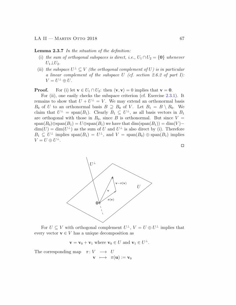
LA II — Martin Otto 2018 67
Lemma 2.3.7 In the situation of the definition:
(i) the sum of orthogonal subspaces is direct, i.e., U1 ∩U2 = {0} wheneverU1⊥U2.
(ii) the subspace U⊥ ⊆ V (the orthogonal complement of U) is in particulara linear complement of the subspace U (cf. section 2.6.2 of part I):V = U⊥ ⊕ U .
Proof. For (i) let v ∈ U1 ∩ U2: then 〈v,v〉 = 0 implies that v = 0.For (ii), one easily checks the subspace criterion (cf. Exercise 2.3.1). It
remains to show that U + U⊥ = V . We may extend an orthonormal basisB0 of U to an orthonormal basis B ⊇ B0 of V . Let B1 = B \ B0. Weclaim that U⊥ = span(B1). Clearly B1 ⊆ U⊥, as all basis vectors in B1
are orthogonal with those in B0, since B is orthonormal. But since V =span(B0)⊕span(B1) = U⊕span(B1) we have that dim(span(B1)) = dim(V )−dim(U) = dim(U⊥) as the sum of U and U⊥ is also direct by (i). ThereforeB1 ⊆ U⊥ implies span(B1) = U⊥, and V = span(B0) ⊕ span(B1) impliesV = U ⊕ U⊥.
2
◦0
U⊥
Uv
GG
π(v)
;;
v−π(v)
SS
For U ⊆ V with orthogonal complement U⊥, V = U ⊕ U⊥ implies thatevery vector v ∈ V has a unique decomposition as
v = v0 + v1 where v0 ∈ U and v1 ∈ U⊥.
The corresponding map π : V −→ Uv 7−→ π(u) := v0
68 Linear Algebra II — Martin Otto 2018
is linear and surjective with kernel U⊥ (check these!). It is called the orthog-onal projection [Orthogonalprojektion] onto U .
Exercise 2.3.2 Show that the orthogonal projection π onto U is a projec-tion, i.e., that π ◦π = π, and that it is uniquely determined by this conditiontogether with the requirement that its image is U and that (v − π(v))⊥Ufor all v.
Exercise 2.3.3 Show that the orthogonal projections of an n-dimensionaleuclidean or unitary space V are precisely those endomorphisms of V thatare represented w.r.t. suitable orthonormal basis by block diagonal matriceswith blocks Ek (0 6 k 6 n) and 0.
Exercise 2.3.4 Consider two subspaces U,W ⊆ V of a euclidean or unitaryspace V , with orthogonal projections πU and πW onto U and W , respectively.Under which conditions is πU ◦ πW an orthogonal projection? Under whichconditions do πU and πW commute?
Observation 2.3.8 An alternative characterisation of orthogonal projectionsis in terms of “best approximations”. Let U ⊆ V be a subspace of a finite-dimensional euclidean or unitary space V , π the orthogonal projection ontoU . Then π(v) is uniquely determined as that vector u in U for which ‖v−u‖is minimal.
Proof. Let π(v) = v0 ∈ U , v − π(v) = v1 ∈ U⊥. We need to show thatfor any u ∈ U , ‖v − u‖ > ‖v1‖ with equality only for u = v0. Express u asu = v0 + w for w ∈ U . Then ‖v− u‖2 = 〈v− u,v− u〉 = 〈v− v0 −w,v−v0−w〉 = 〈v1−w,v1−w〉 = 〈v1,v1〉+ 〈w,w〉 by orthogonality of v1 ∈ U⊥and w ∈ U . Hence ‖v− u‖2 = ‖v1‖2 + ‖w‖2 > ‖v1‖2 with equality only forw = 0.
2
Exercise 2.3.5 Show the following identities in a finite-dimensional euclideanor unitary vector space V , for arbitrary subspaces U,U1, U2 ⊆ V :
(i)(U⊥)⊥ = U .
(ii) (U1 ∩ U2)⊥ = U⊥1 + U⊥2 .
LA II — Martin Otto 2018 69
Exercise 2.3.6 Show that any linear map η : V → F, i.e., any linear form(member of the dual space V ∗ = Hom(V,F)), for a finite-dimensional eu-clidean or unitary space (V, 〈., .〉), can be represented in the form
η : v 7−→ 〈a,v〉
for a suitable a ∈ V . This correspondence induces a canonical isomorphismbetween V ∗ and V for finite-dimensional euclidean or unitary spaces.
2.3.3 Orthogonal and unitary maps
Orthogonal and unitary maps are the automorphisms of euclidean and uni-tary spaces, respectively. So they are vector space automorphisms that arealso isometries of the scalar product (or of the induced norm and metric).
Let us first consider isomorphisms between two euclidean or unitaryspaces, i.e., isometric vector space isomorphisms.
Lemma 2.3.9 Let (V, 〈., .〉V ) and (W, 〈., .〉W ) be two euclidean or two uni-tary spaces. Then the following are equivalent for ϕ ∈ Hom(V,W ):
(i) ϕ is an isomorphism of the euclidean/unitary spaces, i.e., an isometricvector space isomorphism.
(ii) For some (any) orthonormal basis B of V , ϕ(B) = (ϕ(b))b∈B is anorthonormal basis of W .
Proof. Recall that ϕ is a vector space isomorphism iff it transforms abasis of V into a basis of W . It remains to deal with the metric part, ac-cording to Definition 2.1.14. By definition, an isometry preserves the scalarproduct, and hence norms and orthogonality. It therefore maps orthonormalsystems into orthonormal systems. Conversely, the values of the scalar prod-uct are uniquely determined by its values 〈bi,bj〉 on pairs of basis vectors. If,therefore, an orthonormal basis is mapped into an orthonormal basis, thenδij = 〈ϕ(bi), ϕ(bj)〉W = 〈bi,bj〉V = δij guarantee that ϕ preserves scalarproducts. Compare also Corollary 2.3.3.
2
Corollary 2.3.10 Every n-dimensional euclidean vector space V is isomor-phic (isometrically isomorphic) to the n-dimensional standard euclidean spaceRn, and similarly for unitary V and Cn.
70 Linear Algebra II — Martin Otto 2018
Proof. Choose an orthonormal basis in the given euclidean or unitaryspace. The vector space isomorphism that associates these basis vectorswith the standard basis vectors in Rn or Cn, respectively, is an isometry.
2
Definition 2.3.11 Let (V, 〈., .〉) be a euclidean or unitary space, respec-tively. A linear map ϕ ∈ Hom(V, V ) is an orthogonal map [orthogonaleAbbildung] or a unitary map [unitare Abbildung], respectively, if
(i) it is bijective, i.e., a vector space automorphism of V , and
(ii) an isometry of (V, 〈., .〉), i.e., preserves the scalar product.
See Observation 2.1.15 for equivalent characterisations in terms of dis-tance or norm preservation in place of (ii). Orthogonal and unitary mapsalso in particular preserve orthogonality, and in fact can also be characterisedby the property in the lemma above, that they transform orthonormal basesinto orthonormal bases.
Also note that while injectivity of ϕ follows from (ii), surjectivity onlyfollows in the finite-dimensional case. An infinite-dimensional euclidean orunitary space with an orthonormal basis B = (b0,b1,b2, . . .) for instance,has an isometry ϕ : bi 7→ bi+1 for which b0 6∈ image(ϕ).
Example 2.3.12 The following are very common orthogonal maps in theeuclidean spaces R2 and R3:
(i) all rotations about the origin in R2 or about an axis through the originin R3.
(ii) reflections in a line through the origin in R2 or in a plane through theorigin in R3.
Despite their name, orthogonal projections are not orthogonal maps! (Why?)
Exercise 2.3.7 Clearly the identity idV is orthogonal (unitary). Show thatthe composition of any two orthogonal (unitary) maps of (V.〈., .〉) is orthogo-nal (unitary), and that the inverse of an orthogonal (unitary) map is orthog-onal (unitary). Hence, these sets of maps form groups with composition.
Definition 2.3.13 The subgroups of the group Aut(V ) of all vector spaceautomorphisms consisting of just the orthogonal or unitary maps of (V, 〈., .〉)are called the orthogonal group [orthogonale Gruppe] O(V ) (in the euclideancase, over R) and the unitary group U(V ) [unitare Gruppe] (in the unitarycase, over C).
LA II — Martin Otto 2018 71
Orthogonal and unitary matrices
For the unitary case recall that we write A+ for the matrix obtained from Aby simultaneous complex conjugation and transposition. If A = (aij), thenthe entries in A+ are a+ij = aji.
Definition 2.3.14 A regular matrix A ∈ R(n,n) is called orthogonal [orthog-onal] iff At = A−1 (its transpose is its inverse: AAt = AtA = En).
A regular matrix A ∈ C(n,n) is called unitary [unitar] iff A+ = A−1 (itsadjoint is its inverse: AA+ = A+A = En).
Exercise 2.3.8 Show that a matrix A ∈ R(n,n) is orthogonal iff its columnvectors form an orthonormal basis w.r.t. the standard scalar product, iff itsrow vectors form an orthonormal basis w.r.t. the standard scalar product.
Exercise 2.3.9 Show that any change of basis transformation between or-thonormal bases in the standard unitary or euclidean spaces Cn or Rn, re-spectively, are described by unitary or orthogonal matrices, respectively.
Orthogonal (unitary) matrices are precisely the matrix representations oforthogonal (unitary) maps w.r.t. orthonormal bases. They are in particularthe representations of orthogonal (unitary) maps in the standard euclidean(unitary) spaces w.r.t. their standard bases.
Proposition 2.3.15 Let B = (b1, . . . ,bn) be an orthonormal basis of theeuclidean (unitary) space (V, 〈., .〉). Let ϕ ∈ Aut(V ) a vector space automor-phism of V , represented by the matrix A = [[ϕ]]BB ∈ R(n,n) (respectively inC(n,n)). Then the following are equivalent
(i) A is orthogonal (unitary).
(ii) ϕ is orthogonal (unitary).
Proof. We treat the unitary case (its specialisation to real matrices givesthe euclidean analogue). Let A = (aij) be a regular matrix, a+ij = aji be theentries in A+ and recall that we write δij to describe the entries in En, δij = 0for i 6= j and δii = 1.
Now ϕ is an isometry iff ϕ(B) = (ϕ(b1), . . . , ϕ(bn)) is orthonormal, i.e.,iff 〈ϕ(bi), ϕ(bj)〉 = δij. As [[ϕ]]BB = A, ϕ(bi) =
∑k akibk and therefore
〈ϕ(bi), ϕ(bj)〉 = 〈∑
k akibk,∑
` a`jb`〉=
∑k,` akia`j〈bk,b`〉
=∑
k,` akia`jδk` =∑
k akiakj=
∑k a
+ikakj
72 Linear Algebra II — Martin Otto 2018
is the entry in position i, j of A+A. Hence, ϕ = ϕA is an isometry iff〈ϕ(bi), ϕ(bj)〉 = δij iff A+A = En.
2
It follows that the orthogonal, repectively unitary, matrices form groups,in fact subgroups of the general linear groups GLn(R) and GLn(C), respec-tively.
Definition 2.3.16 The matrix groups of orthogonal and unitary matricesare denoted O(n) = O(Rn) ⊆ GLn(R) and U(n) = U(Cn) ⊆ GLn(C).
Isometries of Rn
Isometries of the standard euclidean space Rn are necessarily bijective, andhence orthogonal maps. W.r.t. the standard basis (which is an orthonormalbasis) an isometry ϕ is represented by an orthogonal matrix A = Aϕ ∈ O(n).We now explore the geometric possibilities.
Consider any invariant subspace U ⊆ V of ϕ. By injectivity, ϕ mustmap U onto U (dimension!), and as ϕ preserves orthogonality, U⊥ is alsoan invariant subspace of ϕ. It follows that any invariant subspace of anorthogonal (or unitary) map gives rise to a decomposition into invariantsubspaces that are orthogonal complements and hence allow a diagonal blockdecomposition w.r.t. orthogonal subspaces.
It remains to find invariant subspaces.
(A) If ϕ has an eigenvalue λ, then |λ| = 1 (as ϕ preserves norms). Soλ ∈ {1,−1}. If b is a corresponding eigenvector, then U = span(b) and U⊥
are invariant subspaces. For λ = 1, ϕ is trivial in the direction of b. Forλ = −1, ϕ operates as a reflection in the hyperplane U⊥, combined with theisometric operation of ϕ inside U⊥.
(B) Suppose that ϕ has no (real) eigenvalue. This means that the char-acteristic polynomial p = pϕ = pA has no real zeroes. We then know that nmust be even, and that p must have an irreducible factor which is a prod-uct of two complex conjugate linear factors of p in C[X]. Let this factor be(X − λ)(X − λ) for λ ∈ C \ R, λ = x+ iy, y 6= 0. Consider the map
ϕC : Cn −→ Cnv 7−→ Av
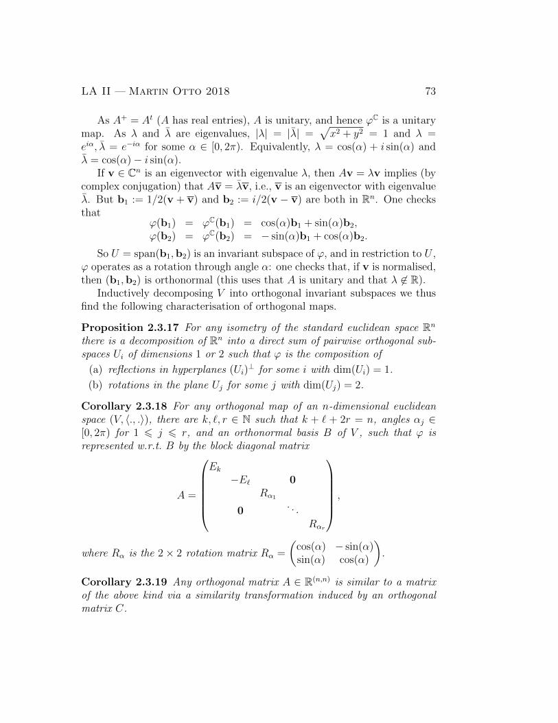
LA II — Martin Otto 2018 73
As A+ = At (A has real entries), A is unitary, and hence ϕC is a unitarymap. As λ and λ are eigenvalues, |λ| = |λ| =
√x2 + y2 = 1 and λ =
eiα, λ = e−iα for some α ∈ [0, 2π). Equivalently, λ = cos(α) + i sin(α) andλ = cos(α)− i sin(α).
If v ∈ Cn is an eigenvector with eigenvalue λ, then Av = λv implies (bycomplex conjugation) that Av = λv, i.e., v is an eigenvector with eigenvalueλ. But b1 := 1/2(v + v) and b2 := i/2(v − v) are both in Rn. One checksthat
ϕ(b1) = ϕC(b1) = cos(α)b1 + sin(α)b2,ϕ(b2) = ϕC(b2) = − sin(α)b1 + cos(α)b2.
So U = span(b1,b2) is an invariant subspace of ϕ, and in restriction to U ,ϕ operates as a rotation through angle α: one checks that, if v is normalised,then (b1,b2) is orthonormal (this uses that A is unitary and that λ 6∈ R).
Inductively decomposing V into orthogonal invariant subspaces we thusfind the following characterisation of orthogonal maps.
Proposition 2.3.17 For any isometry of the standard euclidean space Rnthere is a decomposition of Rn into a direct sum of pairwise orthogonal sub-spaces Ui of dimensions 1 or 2 such that ϕ is the composition of
(a) reflections in hyperplanes (Ui)⊥ for some i with dim(Ui) = 1.
(b) rotations in the plane Uj for some j with dim(Uj) = 2.
Corollary 2.3.18 For any orthogonal map of an n-dimensional euclideanspace (V, 〈., .〉), there are k, `, r ∈ N such that k + ` + 2r = n, angles αj ∈[0, 2π) for 1 6 j 6 r, and an orthonormal basis B of V , such that ϕ isrepresented w.r.t. B by the block diagonal matrix
A =
Ek−E` 0
Rα1
0. . .
Rαr
,
where Rα is the 2× 2 rotation matrix Rα =
(cos(α) − sin(α)sin(α) cos(α)
).
Corollary 2.3.19 Any orthogonal matrix A ∈ R(n,n) is similar to a matrixof the above kind via a similarity transformation induced by an orthogonalmatrix C.
74 Linear Algebra II — Martin Otto 2018
A familiar geometric distinction between a rotation on the one hand, anda reflection in a line of R2 or in a plane of R3 on the other hand, concernstheir behaviour w.r.t. orientation[Orientierung]. An orthonormal basis B =(b1, . . . ,bn) of Rn is said to be positively oriented if
det(b1, . . . ,bn) = 1,
negatively oriented if this determinant is −1.
Exercise 2.3.10 Show that
(i) |A| ∈ {1,−1} for any orthogonal matrix A ∈ R(n,n).
(ii) det(b1, . . . ,bn) ∈ {−1, 1} for any orthonormal basis B = (b1, . . . ,bn)of the standard euclidean space Rn.
Definition 2.3.20 An orthogonal map of the standard space Rn is orien-tation preserving [orientierungserhaltend] if it maps the standard basis (orany other positively oriented orthonormal basis) into a positively orientedorthonormal basis.
An orthogonal matrix A ∈ O(n) ⊆ GLn(R) is called a special orthogonalmatrix if |A| = 1. The special orthogonal matrices form a subgroup of O(n),called the special orthogonal group[spezielle orthogonale Gruppe], denotedSO(n).
Exercise 2.3.11 Show that the special orthogonal matrices are preciselythe representations of the orientation preserving orthogonal maps w.r.t. or-thonormal bases. (Compare Proposition 2.3.15.)
Exercise 2.3.12 Classify all orthogonal maps of R2 and R3 according toProposition 2.3.17 and orientation preservation.
2.4 Endomorphisms in euclidean or unitary
spaces
In this section we study the diagonalisability of endomorphisms of a finite-dimensional euclidean or unitary space. We are interested in matrix repre-sentations of ϕ w.r.t. orthonormal bases and corresponding similarity trans-formations. Recall that a similarity transformation A 7→ A that represents achange from one orthonormal basis of V to another is based on an orthogonalor unitary matrix C for which A = CAC−1.
LA II — Martin Otto 2018 75
2.4.1 The adjoint map
Definition 2.4.1 Let (V, 〈., .〉) be a euclidean or unitary space, ϕ : V → Van endomorphism of V . The endomorphism ϕ+ : V → V is called an adjointof ϕ [adjungierte Abbildung] if for all v,w ∈ V :
〈ϕ(v),w〉 = 〈v, ϕ+(w)〉.
ϕ ∈ Hom(V, V ) is called self-adjoint (or, in the real case, also symmetric)[selbstadjungiert, reell: symmetrisch] if ϕ is its own adjoint.
Observation 2.4.2 For any orthogonal or unitary ϕ, its inverse is its ad-joint.
Proof. Let ϕ ∈ Hom(V, V ) be an isometry, v,w ∈ V . Let w′ :=ϕ−1(w), then the isometry condition that 〈ϕ(v), ϕ(w′)〉 = 〈v,w′〉 impliesthat 〈ϕ(v),w〉 = 〈v, ϕ−1(w)〉.
2
Example 2.4.3 Let V be a finite-dimensional euclidean or unitary space,U ⊆ V a subspace, and consider the orthogonal projection π of V onto U .For an adjoint π+ we need
(i) image(π+) ⊆ (U⊥)⊥ = U .For v ∈ U⊥ and any w ∈ V : 〈v, π+(w)〉 = 〈π(v),w〉 = 〈0,w〉 = 0.
(ii) U⊥ ⊆ ker(π+).For w ∈ U⊥ and any v ∈ V : 〈v, π+(w)〉 = 〈π(v),w〉 = 0.
(iii) π+ ◦ π+ = π+ (i.e., π+ needs to be a projection too).Fix w ∈ W ; then 〈v, π+(π+(w))〉 = 〈π(v), π+(w)〉 = 〈π(π(v)),w〉 =〈π(v),w〉 = 〈v, π+(w)〉 for all v ∈ V implies that π+(π+(w)) = π+(w).
One checks that indeed π+ = π is an adjoint, and that orthogonal projectionsare self-adjoint.
Exercise 2.4.1 Show that ϕ+ is an adjoint of ϕ iff ϕ is an adjoint of ϕ+.
Recall Definition 2.1.8, of self-adjoint (or hermitian) complex matricesA = A+ ∈ C(n,n); their real counterparts, or specialisations, are the symmet-ric real matrices A = At ∈ R(n,n) (note that A+ = At for real A, whence areal self-adjoint matrix is symmetric).
76 Linear Algebra II — Martin Otto 2018
Proposition 2.4.4 For finite-dimensional V : any ϕ ∈ Hom(V, V ) possessesan adjoint and this adjoint is uniquely determined.
In terms of an orthonormal basis B = (b1, . . . ,bn) of V , the adjoint ϕ+
of ϕ is represented by the adjoint matrix of the matrix that represents ϕ:
[[ϕ+]]BB = ([[ϕ]]BB)+.
W.r.t. orthonormal bases, self-adjoint/symmetric endomorphisms are rep-resented by self-adjoint (hermitian)/symmetric matrices.
Proof. We first show uniqueness. Let ψ, ψ′ both be adjoint maps for ϕ.Then
〈ϕ(v),w〉 = 〈v, ψ(w)〉 = 〈v, ψ′(w)〉 for all v ∈ Vimplies that (ψ(w)− ψ′(w))⊥V , hence ψ(w)− ψ′(w) = 0 and ψ = ψ′.
For existence, let B = (b1, . . . ,bn) be an orthonormal basis of V , A =[[ϕ]]BB the matrix representing ϕ. Then the endomorphism ψ whose represen-tation w.r.t. B is A+, is easily seen to satisfy the conditions for an adjoint.Consider v =
∑i λibi and w =
∑j µjbj. Then ϕ(v) =
∑ik akiλibk and
ψ(w) =∑
j` a+`jµjb` =
∑j` aj`µjb`. Therefore
〈ϕ(v),w〉 = 〈∑ik
akiλibk,∑j
µjbj〉 =∑ikj
λiakiµjδkj =∑ij
λiajiµj
and
〈v, ψ(w)〉 = 〈∑i
λibi,∑j`
aj`µjb`〉 =∑ij`
λiaj`µjδi` =∑ij
λiajiµj.
So the equality 〈ϕ(v),w〉 = 〈v, ψ(w)〉 proves that ψ is an adjoint (and hencethe adjoint of ϕ), as well as the claim about its matrix representation.
2
2.4.2 Diagonalisation of self-adjoint maps and matrices
Proposition 2.4.5 Let ϕ = ϕ+ be a self-adjoint endomorphism of the finite-dimensional unitary C-vector space (V, 〈., .〉). Then all eigenvalues of ϕ arereal, and ϕ can be diagonalised w.r.t. an orthonormal basis of V .
Similarly, any self-adjoint (i.e., symmetric) endomorphism of a finite-dimensional euclidean R-vector space is diagonalisable w.r.t. an orthonormalbasis.
LA II — Martin Otto 2018 77
Proof. Let v be an eigenvector with eigenvalue λ ∈ C of ϕ. Then〈ϕ(v),v〉 = λ‖v‖2 = 〈v, ϕ(v)〉 = λ‖v‖2 shows that λ = λ, whence λ ∈ R.
The characteristic polynomial pϕ always splits into linear factors in C[X].As we now see that all these linear factors are of the form (X−λ) for λ ∈ R,pϕ splits into linear factors in R[X] also in the symmetric (real self-adjoint)case.
We claim that (in the euclidean as well as in the unitary case) the orthog-onal complement of an invariant subspace of ϕ is again an invariant subspace.Let U ⊆ V be invariant under ϕ, and let v ∈ U⊥. Then
〈ϕ(v),u〉 = 〈v, ϕ(u)〉 = 0 for all u ∈ U,
since ϕ(u) ∈ U and v⊥U . Hence also ϕ(v) ∈ U⊥.If v is an eigenvector of ϕ, therefore, V = span(v)⊕(span(v))⊥ is a decom-
position into orthogonal complements that are invariant. W.l.o.g. ‖v‖ = 1and we may choose b1 := v as the first basis vector for the desired orthonor-mal basis that diagonalises ϕ. Putting V ′ := (span(v))⊥ and letting ϕ′ bethe restriction of ϕ to V ′, we see that ϕ′ is again self-adjoint, and that we canproceed inductively to select new normalised eigenvectors, each orthogonalon the subspace spanned by the previous. This gives an orthonormal basisw.r.t. which ϕ is represented by a real diagonal matrix (which in particularis self-adjoint of course).
2
Corollary 2.4.6 Any self-adjoint (hermitian) matrix A ∈ C(n,n) is similarto a real diagonal matrix, by means of a similarity transformation based ona unitary matrix: for suitable unitary C, the matrix CAC−1 is diagonal andin R(n,n).
Similarly, any symmetric A ∈ R(n,n) is similar to a diagonal matrix, bymeans of a similarity transformation based on an orthogonal matrix.
Proof. Let A = A+ be given. Consider Cn with its standard scalar prod-uct as a unitary space, and let ϕ = ϕA be the endomorphism that corre-sponds to A w.r.t. the standard basis B0. Then ϕ is self-adjoint, since A isself-adjoint and since the standard basis is orthonormal. By the proposition,there is another orthonormal basis B of Cn such that [[ϕ]]BB is diagonal withreal entries. The basis transformation between the standard basis and thenew B is unitary, as both bases are orthonormal. Hence
[[ϕ]]BB = CAC−1,
78 Linear Algebra II — Martin Otto 2018
where C = [[id]]B0B is the unitary matrix whose column vectors consist of the
coefficients of the standard basis vectors w.r.t. the new orthonormal basis B,[[ej]]B.
In the real case, the corresponding basis transformation similarly is de-scribed by an orthogonal matrix C.
2
2.4.3 Normal maps and matrices
Propositions 2.4.5 and 2.3.17 both essentially used the fact that the orthogo-nal complement of the invariant subspace spanned by an eigenvector wasagain an invariant subspace. The following classes of normal endomor-phisms and matrices provide a common generalisation that includes uni-tary/orthogonal as well as self-adjoint/symmetric maps or matrices.
Definition 2.4.7 (i) An endomorphism ϕ ∈ Hom(V, V ) of a euclidean orunitary space (V, 〈., .〉) is called normal [normal] if ϕ and its adjointϕ+ commute:
ϕ+ ◦ ϕ = ϕ ◦ ϕ+.
(ii) A matrix A ∈ C(n,n) is called normal if it commutes with its adjoint:
A+A = AA+.
Lemma 2.4.8 Let (V, 〈., .〉) be euclidean or unitary with orthonormal basisB = (b1, . . . ,bn). Let ϕ ∈ Hom(V, V ) be represented w.r.t. B by the matrixA = [[ϕ]]BB Then the following are equivalent:
(i) ϕ is normal.
(ii) A is normal.
Proof. Straightforward calculation, similar to the corresponding part inthe proof of Proposition 2.4.4.
2
The following combines observations about the correspondence of uni-tary/orthogonal or self-adjoint/symmetric maps with the corresponding ma-trices. Also observe that trivially, A commutes with A and, for regular A,also with A−1.
LA II — Martin Otto 2018 79
Observation 2.4.9 The following classes of matrices in particular are nor-mal:
(i) unitary (in the euclidean case, for F = R: orthogonal) matrices.
(ii) self-adjoint (in the euclidean case, for F = R: symmetric) matrices.
Analogously, the following classes of endomorphisms are normal:
(i) unitary and orthogonal maps, respectively.
(ii) self-adjoint and symmetric maps, respectively.
Diagonalisation over C
Theorem 2.4.10 Let (V, 〈., .〉) be a finite-dimensional unitary space, ϕ ∈Hom(V, V ) normal. Then ϕ is diagonalisable w.r.t. an orthonormal basis for(V, 〈., .〉).
Proof. Note that, as we are working over C, ϕ does have an eigenvalueλ. We claim that the (non-trivial) eigenspace Vλ ⊆ V of ϕ is an invariantsubspace also for ϕ+. Let v ∈ Vλ, i.e., ϕ(v) = λv. We need to show thatalso ϕ+(v) ∈ Vλ. By normality, ϕ(ϕ+(v)) = ϕ+(ϕ(v)) = ϕ+(λv) = λϕ+(v)shows that indeed ϕ+(v) ∈ Vλ.
Therefore, ϕ+ will also have an eigenvector w ∈ Vλ (look at the restrictionof ϕ+ to Vλ). Any such w therefore is a simultaneous eigenvector of bothϕ and ϕ+: ϕ(w) = λw and ϕ+(w) = γw. As γ‖w‖2 = 〈w, ϕ+(w)〉 =〈ϕ(w),w〉 = λ‖w‖2, it follows that γ = λ.
We next argue that for any such simultaneous eigenvector w, both W =span(w) and its orthogonal complement V ′ := W⊥ are invariant subspacesfor ϕ and ϕ+. This is clear for W ; so consider W⊥, and for instance invarianceunder ϕ. For a ∈ W⊥ we need to show that ϕ(a) ∈ W⊥, i.e., that ϕ(a)⊥W ,or that 〈ϕ(a),w〉 = 0. But 〈ϕ(a),w〉 = 〈a, ϕ+(w)〉 = γ〈a,w〉 = 0 sincea⊥w. Similarly, for invariance under ϕ+, use that 〈ϕ+(a),w〉 = 〈a, ϕ(w)〉 =λ〈a,w〉.
Hence, the desired orthonormal basis B = (b1, . . . ,bn) is found induc-tively, as follows. For a first basis vector b1 pick any normalised simultane-ous eigenvector w of ϕ and ϕ+. Let W = span(b1) and V ′ := W⊥ so thatV = W ⊕ V ′, W⊥V ′ are orthogonal complements.
As W and W⊥ are both invariant under ϕ and ϕ+, the restrictions of ϕand ϕ+ to V ′ are adjoints of each other, and normal. Any extension of b1 toan (orthonormal) basis of V by an (orthonormal) basis of V ′ will lead to a
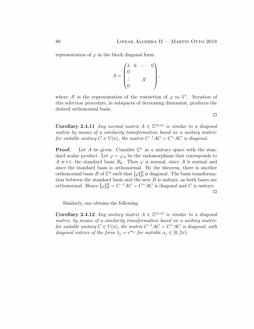
80 Linear Algebra II — Martin Otto 2018
representation of ϕ in the block diagonal form
A =
λ 0 · · · 00... A′
0
,
where A′ is the representation of the restriction of ϕ to V ′. Iteration ofthis selection procedure, in subspaces of decreasing dimension, produces thedesired orthonormal basis.
2
Corollary 2.4.11 Any normal matrix A ∈ C(n,n) is similar to a diagonalmatrix by means of a similarity transformation based on a unitary matrix:for suitable unitary C ∈ U(n), the matrix C−1AC = C+AC is diagonal.
Proof. Let A be given. Consider Cn as a unitary space with the stan-dard scalar product. Let ϕ = ϕA be the endomorphism that corresponds toA w.r.t. the standard basis B0. Then ϕ is normal, since A is normal andsince the standard basis is orthonormal. By the theorem, there is anotherorthonormal basis B of Cn such that [[ϕ]]BB is diagonal. The basis transforma-tion between the standard basis and the new B is unitary, as both bases areorthonormal. Hence [[ϕ]]BB = C−1AC = C+AC is diagonal and C is unitary.
2
Similarly, one obtains the following.
Corollary 2.4.12 Any unitary matrix A ∈ C(n,n) is similar to a diagonalmatrix, by means of a similarity transformation based on a unitary matrix:for suitable unitary C ∈ U(n), the matrix C−1AC = C+AC is diagonal, withdiagonal entries of the form λj = eiαj for suitable αj ∈ [0, 2π).
Chapter 3
Bilinear and Quadratic Forms
In this chapter we restrict attention to finite-dimensional R-vector spaces andeuclidean spaces. Unless stated otherwise, let (V, 〈., .〉) be an n-dimensionaleuclidean space.
3.1 Matrix representations of bilinear forms
Recall from section 2.1.3 how we represent a bilinear form σ : V × V → Rover an n-dimensional R-vector space V w.r.t. a basis B = (b1, . . . ,bn) bythe matrix A = [[σ]]B = (aij) with entries
aij = σ(bi,bj).
If v =∑
i λibi and w =∑
j µjbj, then σ is evaluated on these argumentsaccording to
σ(v,w) =∑ij
λiaijµj = (λ1, . . . , λn)A
µ1...µn
= [[v]]tB[[σ]]B[[w]]B.
If B′ = (b′1, . . . ,b′n) is another basis, and if the corresponding basis trans-
formation from B′ to B is described by the matrix C = (cij) = [[idV ]]B′
B suchthat b′i =
∑k ckibk, then the matrix A′ = [[σ]]B
′= (a′ij) that represents σ
81
82 Linear Algebra II — Martin Otto 2018
w.r.t. B′ has entries
a′ij = σ(b′i,b′j) = σ(
∑k ckibk,
∑` c`jb`)
=∑
k` ckic`jσ(bk,b`) =∑
k` ckiak`c`j=
(CtAC
)ij,
or [[σ]]B′
= ([[idV ]]B′
B )t[[σ]]B[[idV ]]B′
B .
Observation 3.1.1 As representations of bilinear forms matrices A ∈ R(n,n)
transform under changes of basis according to
A 7−→ CtAC,
for C ∈ GLn(R) (regular matrices).Note how this differs from the transformation pattern for matrices as
representations of endomorphisms, which is A 7→ C−1AC. If C, however, isorthogonal (C ∈ O(n), cf. Definitions 2.3.14 and 2.3.16: Ct = C−1), thenthese two transformations coincide.
Exercise 3.1.1 Show that the relation ≈ on R(n,n) defined as A ≈ A′ iffA′ = CtAC for some C ∈ GLn(R) is an equivalence relation. What aresufficient criteria for A 6≈ A′?
3.2 Simultaneous diagonalisation
We have seen in the previous chapter that certain endomorphisms of a eu-clidean space (V, 〈., .〉) can be diagonalised w.r.t. an orthonormal basis. An-other way of saying that is that the underlying scalar product 〈., .〉 and thegiven endomorphism ϕ : V → V can simultaneously be diagonalised: anorthonormal basis (by definition) leads to a diagonal matrix for the represen-tation of the scalar product, namely the unit matrix En; and at the same timeprovides a diagonal matrix for the representation of ϕ. In particular that wasseen to be possible for self-adjoint endomorphisms, see Proposition 2.4.5.
A similar question can be asked about the given scalar product and a sec-ond symmetric bilinear form σ on V : when is it possible to find one basis thatsimultaneously represents both, 〈., .〉 and σ by diagonal matrices? Equiva-lently, when can σ be represented by a diagonal matrix w.r.t. an orthonormalbasis of (V, 〈., .〉)? These questions in fact reduce to what we already knowabout self-adjoint diagonalisation of endomorphism.
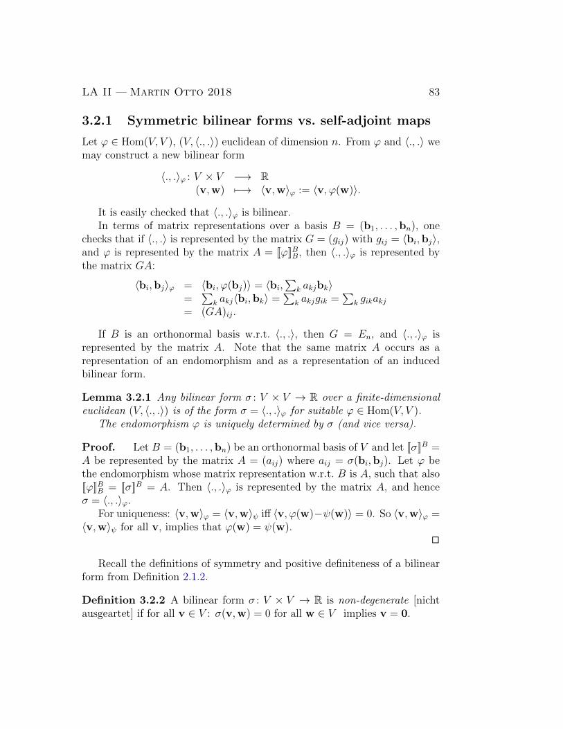
LA II — Martin Otto 2018 83
3.2.1 Symmetric bilinear forms vs. self-adjoint maps
Let ϕ ∈ Hom(V, V ), (V, 〈., .〉) euclidean of dimension n. From ϕ and 〈., .〉 wemay construct a new bilinear form
〈., .〉ϕ : V × V −→ R(v,w) 7−→ 〈v,w〉ϕ := 〈v, ϕ(w)〉.
It is easily checked that 〈., .〉ϕ is bilinear.In terms of matrix representations over a basis B = (b1, . . . ,bn), one
checks that if 〈., .〉 is represented by the matrix G = (gij) with gij = 〈bi,bj〉,and ϕ is represented by the matrix A = [[ϕ]]BB, then 〈., .〉ϕ is represented bythe matrix GA:
〈bi,bj〉ϕ = 〈bi, ϕ(bj)〉 = 〈bi,∑
k akjbk〉=
∑k akj〈bi,bk〉 =
∑k akjgik =
∑k gikakj
= (GA)ij.
If B is an orthonormal basis w.r.t. 〈., .〉, then G = En, and 〈., .〉ϕ isrepresented by the matrix A. Note that the same matrix A occurs as arepresentation of an endomorphism and as a representation of an inducedbilinear form.
Lemma 3.2.1 Any bilinear form σ : V × V → R over a finite-dimensionaleuclidean (V, 〈., .〉) is of the form σ = 〈., .〉ϕ for suitable ϕ ∈ Hom(V, V ).
The endomorphism ϕ is uniquely determined by σ (and vice versa).
Proof. Let B = (b1, . . . ,bn) be an orthonormal basis of V and let [[σ]]B =A be represented by the matrix A = (aij) where aij = σ(bi,bj). Let ϕ bethe endomorphism whose matrix representation w.r.t. B is A, such that also[[ϕ]]BB = [[σ]]B = A. Then 〈., .〉ϕ is represented by the matrix A, and henceσ = 〈., .〉ϕ.
For uniqueness: 〈v,w〉ϕ = 〈v,w〉ψ iff 〈v, ϕ(w)−ψ(w)〉 = 0. So 〈v,w〉ϕ =〈v,w〉ψ for all v, implies that ϕ(w) = ψ(w).
2
Recall the definitions of symmetry and positive definiteness of a bilinearform from Definition 2.1.2.
Definition 3.2.2 A bilinear form σ : V × V → R is non-degenerate [nichtausgeartet] if for all v ∈ V : σ(v,w) = 0 for all w ∈ V implies v = 0.
84 Linear Algebra II — Martin Otto 2018
Note that positive definiteness implies non-degeneracy, but non-degen-eracy is strictly weaker and in particular makes sense also for forms thatproduce negative values for some σ(v,v).
Lemma 3.2.3 Over a finite dimensional euclidean space (V, 〈., .〉) and forany ϕ ∈ Hom(V, V ):
(i) 〈., .〉ϕ is non-degenerate iff ϕ is regular (rank(ϕ) = dim(V )).
(ii) 〈., .〉ϕ is symmetric iff ϕ is self-adjoint.
Proof. For (i): 〈v,w〉ϕ = 0 iff 〈v, ϕ(w)〉 = 0 iff v⊥ϕ(w). Hence 〈v,w〉ϕ =0 for all w iff v⊥ image(ϕ).
If ϕ is regular, then image(ϕ) = V and v⊥ image(ϕ) implies v = 0.Otherwise, any v ∈ image(ϕ)⊥ \ {0} demonstrates that 〈., .〉ϕ is degener-
ate.
For (ii), recall that the adjoint ϕ+ of ϕ is defined by the condition that
〈v, ϕ+(w)〉 = 〈ϕ(v),w〉,
which now gives
〈w,v〉ϕ = 〈w, ϕ(v)〉 = 〈ϕ(v),w〉 = 〈v, ϕ+(w)〉 = 〈v,w〉ϕ+ .
Uniqueness in Lemma 3.2.1 shows that 〈., .〉ϕ is symmetric iff ϕ = ϕ+. Alter-natively, one may also consider the matrix representations w.r.t. an orthonor-mal basis and use the fact that symmetry of a bilinear form correspondsto symmetry of its matrix representation (w.r.t. arbitrary bases); and thatself-adjoint endomorphisms are represented by self-adjoint (i.e., symmetric)matrices w.r.t. orthonormal bases.
2
Exercise 3.2.1 Show that ϕ is regular iff ϕ+ is regular.
3.2.2 Principal axes
Definition 3.2.4 Let B = (b1, . . . ,bn) be a basis of V , and σ a bilinear formwhich is represented by a diagonal matrix w.r.t. basis B: σ(bi,bj) = λiδijfor suitable λj ∈ R. Then the one-dimensional subspaces spanned by basisvectors bi are called principal axes [Hauptachsen] for σ.
LA II — Martin Otto 2018 85
Note that principal axes of σ are characterised by pairwise ‘orthogonalityw.r.t. σ’. It turns out that any symmetric bilinear form σ has such principalaxes. Moreover these can always be chosen orthogonal w.r.t. a given scalarproduct in V .
A non-trivial application in physics involves the diagonalisation of themoment of inertia of a rigid body, which is crucial for its equations of motionin classical mechanics; this is discussed in the appendix, see section 3.3.3.
Theorem 3.2.5 Any symmetric bilinear form σ over a finite-dimensionaleuclidean space (V, 〈., .〉) can be diagonalised w.r.t. an orthonormal basis of(V, 〈., .〉). I.e., there is an orthonormal basis B = (b1, . . . ,bn) of (V, 〈., .〉)such that σ is represented by a diagonal matrix w.r.t. B: σ(bi,bj) = λiδijfor suitable λi.
Proof. The claim reduces to our results on diagonalisation of self-adjoint(symmetric) endomorphisms, if we go via a presentation of σ as σ = 〈., .〉ϕfor a self-adjoint ϕ.
By Proposition 2.4.5, we have an orthonormal basis B = (b1, . . . ,bn) of(V, 〈., .〉) such that the endomorphism ϕ is represented by a diagonal matrixD = [[ϕ]]BB:
D =
λ1 0. . .
0 λn
.
Since 〈., .〉 is represented by En w.r.t. B, σ = 〈., .〉ϕ is also represented by Dw.r.t. B.
2
If we consider diagonalisation w.r.t. bases that are not necessarily or-thonormal, then the actual diagonal entries λi are clearly not determined byσ. A rescaling of basis vector bi to b′i = αbi, α 6= 0, changes λi into α2λi.However, the sign distribution of the λi is an invariant.
Theorem 3.2.6 (Sylvester) Let σ be a symmetric bilinear form over thefinite-dimensional R-vector space V . For any basis B = (b1, . . . ,bn) of Vsuch that σ is represented by a diagonal matrix with entries σ(bi,bj) = λiδijfor suitable λi, the numbers of λi that are positive, negative, and equal to 0,respectively, are uniquely determined by σ (independent of B).
86 Linear Algebra II — Martin Otto 2018
Proof. Let s be the number of positive λi, t the number of negative λi,and consequently d := n − s − t the number of i for which λi = 0. W.l.o.g.assume that σ(bi,bi) > 0 for i = 1, . . . , s; σ(bi,bi) < 0 for i = s+1, . . . , s+t;σ(bi,bi) = 0 for i = s+ t+ 1, . . . , n.
One checks that d, the number of λi = 0, is the dimension of the subspace
U0 = {u ∈ V : σ(u,v) = 0 for all v ∈ V },
hence independent of B.We claim that the number s of positive λi is the dimension of a maximal
subspace U+ ⊆ V on which the restriction of σ is positive definite. ClearlyV has an s-dimensional subspace on which σ is positive definite, namelyspan(b1, . . . ,bs). It therefore suffices to show that if σ is positive definite inrestriction to U ⊆ V , then dim(U) 6 s. Otherwise U ∩ span(bs+1, . . . ,bn) 6={0}. But then there is a u ∈ U \ {0} for which σ(u,u) 6 0, contradictingpositive definiteness.
Since we have found basis independent characterisations for the numbersn− s− t and s, and since t is uniquely determined by n and these, the claimis proved.
2
Definition 3.2.7 The signature [Signatur] of a symmetric bilinear form is
(+s,−t, 0d) = (+, . . . ,+︸ ︷︷ ︸s
,−, . . . ,−︸ ︷︷ ︸t
, 0, . . . , 0︸ ︷︷ ︸d=n−s−t
)
where the numbers s, t, d are determined according to the theorem as thenumber of λi in any diagonal representation of σ that are positive, negative,or equal to 0, respectively.
Exercise 3.2.2 Show that σ is non-degenerate iff its signature consists of 1and −1 only, without 0.
Corollary 3.2.8 For a symmetric bilinear form σ of signature (+s,−t, 0d)over (V, 〈., .〉): there is a basis consisting of pairwise orthogonal basis vectorssuch that σ is represented by the diagonal matrix
A =
Es −Et0
.
LA II — Martin Otto 2018 87
Proof. Diagonalise σ w.r.t. an orthonormal basis B, according to Theo-rem 3.2.5. A further rescaling of these basis vectors according to
bi :=
1√
σ(bi,bi)bi if σ(bi,bi) > 0
1√−σ(bi,bi)
bi if σ(bi,bi) < 0
bi if σ(bi,bi) = 0
and permutation of the bi if necessary, produces the desired result.2
In terms of matrices, the above considerations correspond to the following.
Proposition 3.2.9 Let A ∈ R(n,n) be symmetric (At = A). Then there isan orthogonal matrix C ∈ O(n) ⊆ GLn(R) such that CtAC = C−1AC isdiagonal.
With C ∈ GLn(R) one correspondingly achieves diagonal CtAC with en-tries from {1,−1, 0}. The numbers of entries 1, −1 and 0, respectively, inany such representation are uniquely determined.
Proof. Regard A as the representation of a corresponding symmetric bi-linear form σA : (v,w) 7→ vtAw. This means that A represents σA w.r.t. thestandard basis of Rn, which is an orthonormal basis of the standard scalarproduct. By Theorem 3.2.5, there is also an orthonormal basis such that σAis represented by a diagonal matrix D. Since the change of basis involvedmaps one orthonormal basis into another, the transformation is effected byan orthogonal matrix C ∈ O(n). We therefore have D = CtAC = C−1ACdiagonal as claimed.
The second point is similarly obtained with the help of Corollary 3.2.8and Theorem 3.2.6.
2
Exercise 3.2.3 Compare Definition 3.2.10 below for positive definiteness ofa symmetric matrix G ∈ R(n,n).
Show that for two symmetric matrices A,G ∈ R(n,n) such that G ∈ R(n,n)
is also positive definite, there is some C ∈ GLn(R) such that CtAC andCtGC are both diagonal.[Hint: regard G as the representation of a scalar product over Rn, and thenproceed as above.]
88 Linear Algebra II — Martin Otto 2018
3.2.3 Positive definiteness
Recall that a bilinear form σ on V is positive definite if σ(v,v) > 0 for allv ∈ V and if σ(v,v) = 0 implies v = 0.
Definition 3.2.10 For a symmetric matrix A ∈ R(n,n), A = (aij)16i,j6n:
(i) A is positive definite if the bilinear form (v,w) 7→ vtAw is positivedefinite on Rn, i.e., if vtAv > 0 for all v ∈ Rn and vtAv = 0 only forv = 0.
(ii) The k-th principal minor [Hauptminor] of A, for k = 1, . . . , n, is thematrix
Ak = (aij)16i,j6k ∈ R(k,k),
the restriction of A to the first k rows and columns.
Part (i) of the definition is just such that a symmetric bilinear σ thatis represented by the symmetric matrix A w.r.t. some basis of V is positivedefinite iff A is positive definite.
The following establishes criteria that can be useful in determining whethera given bilinear form or symmetric matrix is positive definite.
Proposition 3.2.11 The following are equivalent for any symmetric matrixA ∈ R(n,n):
(i) A is positive definite.
(ii) There is an orthogonal matrix C such that CtAC(= C−1AC) is diago-nal with positive entries on the diagonal.
(iii) All eigenvalues of A are positive (A viewed as the representation of anendomorphism of Rn).
(iv) All principal minors of A have positive determinant: |Ak| > 0 for k =1, . . . , n.
Proof. Clearly the symmetric bilinear form represented by some diagonalmatrix is positive definite iff the diagonal entries are all positive.
As any symmetric bilinear form and symmetric matrix can be diagonalisedby means of an orthogonal change of basis transformation, the equivalencebetween (i),(ii) and (iii) is clear. [Note that CtAC = C−1AC means that Ais diagonalised in both its roles, as a representation of a symmetric bilinearform and as a representation of an endomorphism!]
LA II — Martin Otto 2018 89
(i) ⇒ (iv). Let σ be the symmetric bilinear form on Rn defined byσ(v,w) = vtAw (the symmetric bilinear form over Rn represented by Aw.r.t. the standard basis). Then Ak represents the restriction of σ to the k-dimensional subspace spanned by the first k standard basis vectors of Rn. IfA and hence σ are positive definite, so are these restrictions. Now Ak can bediagonalised by means of an orthogonal C ∈ O(k). Let CtAkC = C−1AkC bediagonal with diagonal entries λ1, . . . , λk. By positive definiteness, all λi > 0.Hence 0 <
∏ki=1 λi = |C−1AkC| = |Ak|.
(iv) ⇒ (i) is shown by induction on n. Base case, n = 1. In this case,A = a ∈ R and (iv) says that a > 0, hence positive definite.
Induction step n → n + 1. Let A ∈ R(n+1,n+1) be symmetric and letσ be the symmetric bilinear form over Rn+1 represented by A w.r.t. thestandard basis. Consider the n-th principal minor An of A, which representsthe restriction of σ to the n-dimensional subspace of Rn+1 spanned by thefirst n standard basis vectors. Since |Ak| > 0 for k = 1, . . . , n, the inductionhypothesis implies that this restriction of σ is positive definite.
Let U+ ⊆ Rn+1 be a maximal subspace on which σ is positive definiteand containing the first n standard basis vectors. Suppose there is also anon-trivial subspace U0 such that σ(u,u) 6 0 for all u ∈ U0. It follows thatU0 ∩ U+ = {0}, as any v ∈ (U0 ∩ U+) \ {0} would have to have σ(v,v) > 0and σ(v,v) 6 0. So dim(U0) 6 1.
Therefore diagonalising A with an orthogonal C ∈ O(n + 1), we get adiagonal matrix A′ = CtAC = C−1AC with at most one diagonal entry thatis non-positive. If A′ had indeed one diagonal entry λ 6 0 then |A′| 6 0. But|A′| = |C−1AC| = |A| = |An| > 0 by assumption. Therefore all the diagonalentries of A′ are positive, and σ is positive definite.
2
3.3 Quadratic forms and quadrics
Let σ : V × V → R be a symmetric bilinear form. With it associate theinduced function
Q : V −→ Rv 7−→ Q(v) := σ(v,v).
Such a function is called a quadratic form, as defined below.Note that for positive definite σ, this is just the square of the positive
definite norm associated with σ.
90 Linear Algebra II — Martin Otto 2018
Definition 3.3.1 A function Q : V → R over the R-vector space V is aquadratic form [quadratische Form] if
(i) for all v ∈ V and λ ∈ R: Q(λv) = λ2Q(v).
(ii) the map
σQ : V × V −→ R(v,w) 7−→ σQ(v,w) := 1/2(Q(v + w)−Q(v)−Q(w))
is (symmetric and) bilinear.
Clearly there is a one-to-one correspondence between quadratic forms andsymmetric bilinear forms: according to (ii) in the definition, a quadratic formQ has an associated symmetric bilinear form σQ.
Observation 3.3.2 For a quadratic form Q there is precisely one symmetricbilinear form σ such that Q(v) = σ(v,v) for all v ∈ V .
Proof. Clearly σ := σQ as in (ii) of the definition is as desired. Foruniqueness observe that Q(v) = σ(v,v) for symmetric σ implies that
Q(v + w) = σ(v + w,v + w) = σ(v,v) + σ(w,w) + σ(v,w) + σ(w,v)= Q(v) +Q(w) + 2σ(v,w).
Hence σ(v,w) = 1/2(Q(v + w)−Q(v)−Q(w)) is recovered from Q.2
The matrix representation of the quadratic form Q w.r.t. basis B =(b1, . . . ,bn) is the symmetric matrix that represents σQ, with entries
qij = σQ(bi,bj) =1
2(Q(bi + bj)−Q(bi)−Q(bj)).
Example 3.3.3 The quadratic form associated with the standard scalarproduct in Rn is Q((x1, . . . , xn)) =
∑i x
2i , the square of the standard eu-
clidean norm.For c ∈ R, the quadratic equation
Q(x) =∑i
x2i = c
defines
LA II — Martin Otto 2018 91
(i) for c > 0: a sphere of radius√c in Rn.
Especially, for c = 1, the unit sphere Sn−1 ⊆ Rn.
(ii) for c < 0: the empty set.
(iii) for c = 0: the singleton set {0}.
Example 3.3.4 For the symmetric bilinear form σ((x, y), (x′, y′)) = xx′−yy′over R2, the associated quadratic form is Q(x, y) = x2 − y2.
For c ∈ R, the quadratic equation
Q(x) = x2 − y2 = c
defines
(i) for c 6= 0: a hyperbola (with two branches), symmetric w.r.t. the x- andy-axes:
Xc = {(x, y) ∈ R2 : x2 − y2 = c} = {(x, y) ∈ R2 : x+ y =c
x− y},
with asymptotic lines x+ y = 0 and x− y = 0.
(ii) for c = 0: the union of the two lines x+ y = 0 and x− y = 0.
We now use the principal axes of the associated bilinear form σQ in orderto analyse the geometry of Q. W.l.o.g. we consider Rn with the standardscalar product.
Proposition 3.3.5 Let Q be a quadratic form on Rn. Then there are anorthonormal basis B = (b1, . . . ,bn) of (Rn, 〈., .〉) and numbers λ1, . . . , λn ∈ Rsuch that for x =
∑i xibi:
Q(x) =n∑i=1
λi x2i .
Proof. Direct from Theorem 3.2.5, for σ := σQ.2
Geometrically, a rescaling of the basis vectors from some orthonormalbasis (with positive real factors) corresponds to distortions in the directionof the orthogonal axes given by these basis vectors. Just as in Corollary 3.2.8,we thus find that, up to such a rescaling and with a permutation of the basisvectors, any quadratic form is representable as follows.
92 Linear Algebra II — Martin Otto 2018
Corollary 3.3.6 For every quadratic form Q over Rn there are a basis ofpairwise orthogonal (but not necessarily normalised) vectors bi and numberss, t ∈ N such that k := s+ t 6 n, such that in terms of coordinates w.r.t. thisbasis, Q is given by
Q(x1, . . . , xn) =s∑i=1
x2i −k∑
i=s+1
x2i .
The signature of the quadratic form Q is defined, in accordance withthe definition for symmetric bilinear forms, to be (+s,−t, 0d), for s, t andd = n− s− t as in the corollary.
In connection with equations of motion of rigid body in R3, to be discussedin the appendix, see section 3.3.3, the rotational kinetic energy is expressedby a (positive definite) quadratic form that maps the momentary angularvelocity to the rotational energy, and this quadratic form is derived fromthe symmetric bilinear form induced by the moment of inertia, which (as alinear map) also relates the angular velocity to the angular momentum: therelationship between these two roles of the moment of inertia is as discussedin section 3.2.1 above.
3.3.1 Quadrics in Rn
Definition 3.3.7 A quadric [Quadrik] X ⊆ Rn is a subset defined by aquadratic equation
X ={x ∈ Rn : xtAx + btx + c = 0
},
where A ∈ R(n,n) is a symmetric matrix, b ∈ Rn and c ∈ R.
We may think of a quadric X as being defined in terms of an associatedquadratic form Q(x) = xtAx with matrix representation A, a linear formη(x) = btx = 〈b,x〉, and a constant term c ∈ R.
Exercise 3.3.1 Show that any quadratic equation over Rn, of the form∑16i,j6n
αijxixj +∑16i6n
βixi + γ = 0
for arbitrary αij, βi, γ ∈ R, can be represented in the form xtAx+btx+c = 0for a suitable symmetric matrix A and suitable b and c.
LA II — Martin Otto 2018 93
Example 3.3.8 We classify the quadrics without linear terms (b = 0)
X = {x ∈ R3 : Q(x) = c} ⊆ R3,
up to bijective linear transformations. Note that quadrics without linearterms are invariant under central reflection in 0, so that 0 may play a specialrole as a centre of symmetry (absence of linear terms is not invariant undertranslations). It turns out that the signature of the quadratic form and acase distinction w.r.t. c = 0, c > 0, or c < 0 determines the type of X (upto linear transformations). Since a simultaneous change of sign in c and inthe signature leaves X invariant, need consider only the signatures (+,+,+),(+,+,−), (+,+, 0), (+,−, 0), (+, 0, 0) and (0, 0, 0). We thus look at thesecases:
Signature (+,+,+). σQ is positive definite. In a suitable orthonormal basisQ(x, y, z) = αx2 + βy2 + γz2, where α, β, γ > 0.
For c < 0 the quadric is empty; for c = 0 it consists of just the null vector.For c > 0 the quadric
X = {(x, y, z) ∈ R3 : αx2 + βy2 + γz2 = c}
is an ellipsoid , which may be regarded as the image of the unit sphere S2 ⊆ R3
under the transformation
(x, y, z) 7−→ (√c/α x,
√c/β y,
√c/γ z).
Up to linear transformations, X is the unit sphere.
Signature (+,+,−). In a suitable orthonormal basis Q(x, y, z) = αx2+βy2−γz2, where α, β, γ > 0.
Through normalisation with factors√|c|/α,
√|c|/β,
√|c|/γ, the quadric
transforms intoX = {(x, y, z) : x2 + y2 − z2 = c},
where c ∈ {0, 1,−1}. Note that X is rotation symmetric about the z-axis;note that x2 + y2 is the square of the radial distance of (x, y, z) from thez-axis.
For c = 0, X is the cone {x = (x, y, z) : x2 + y2 = z2}.For c = 1, X = {(x, y, z) : x2 + y2 = 1 + z2} is the surface generated by
rotation about the z-axis from the hyperbola [Hyperbel] in the x-z-plane
{(x, z) ∈ R2 : x2 = 1 + z2} = {(x, z) ∈ R2 : x+ z =1
x− z}.
94 Linear Algebra II — Martin Otto 2018
This is called a single-sheet hyperboloid (‘single-sheet’ because it has one con-nected component). Interestingly, the same surface is generated by rotationof the line
{(1, 0, 0) + λ(0, 1, 1) : λ ∈ R}about the z-axis.
For c = −1, X = {(x, y, z) : x2 + y2 = z2 − 1} is the surface generated byrotation about the z-axis from the hyperbola in the x-z-plane
{(x, z) ∈ R2 : z2 − x2 = 1} = {(x, z) ∈ R2 : z + x =1
z − x},
a two-sheet hyperboloid (‘two-sheet’ because of the two connected compo-nents).
Signature (+,+, 0). In a suitable orthonormal basis Q(x, y, z) = αx2 + βy2,where α, β > 0.
For c < 0, the quadric X is empty, for c = 0 it consists of the z-axis.For c > 0, the quadric is an elliptic cylinder , erected in the direction of
the z-axis over the ellipse {(x, y) : αx2 + βy2 = 0} in the x-y-plane. Up tolinear transformations it is equivalent to the standard cylinder
X = {(x, y, z) : x2 + y2 = 1}.
Signature (+,−, 0). In a suitable orthonormal basis Q(x, y, z) = αx2 − βy2,where α, β > 0, and after transformation with corresponding factors,
X = {(x, y, z) : x2 − y2 = c},
where c ∈ {0,−1, 1}.For c = 0, X is the union of the two planes defined by x = y and x = −y,
respectively.For c = 1 or −1, X is a cylinder erected in the z-direction over suitable
hyperbolas in the x-y-plane.
Signature (+, 0, 0). In a suitable orthonormal basis Q(x, y, z) = αx2, α > 0.For c = 0 the quadric X consists of the y-z-plane, defined by x = 0.For c < 0, X = ∅.For c > 0, X consists of two parallel planes, defined by x = ±
√c/α.
Signature (0, 0, 0). Q(x, y, z) = 0; for c = 0 the quadric X is the whole space,otherwise it is empty.
LA II — Martin Otto 2018 95
We shall further classify also all quadrics with linear terms over R2 below.For that however, it will be convenient to regard them in the context ofprojective spaces, which will simplify the analysis.
Consider the general quadric
X ={x ∈ Rn : xtAx + btx + c = 0}.
For the geometric study of X as a subset of Rn, we now consider asequivalence transformations all linear transformations (arbitrary choice ofbasis) and translations (arbitrary choice of an origin). In other words, wework up to affine rather than just up to linear transformations for the sakeof a more uniform analysis.
Let Q(x) = xtAx be the associated quadratic form, (+s,−t, 0n−s−t) thesignature of Q. Put k := s+ t. By a suitable choice of basis (orthogonal butnot necessarily orthonormal) in Rn, we may assume that A is diagonal withnon-zero entries aii = 1 for i = 1, . . . , s and aii = −1 for i = s+ 1, . . . , k. Sow.o.l.g.
X ={x ∈ Rn :
∑si=1 x
2i −
∑ki=s+1 x
2i +
∑ni=1 bixi + c = 0
}.
We now use a translation to further simplify the linear term∑
i bixi. Atranslation through vector −u for u = (u1, . . . , un) ∈ Rn transforms X into{x : x + u ∈ X}, defined by the equation∑s
i=1(xi + ui)2 −
∑ki=s+1(xi + ui)
2 +∑n
i=1 bi(xi + ui) + c = 0,
which is equivalent to∑si=1 x
2i −
∑ki=s+1 x
2i [quadratic]
+∑s
i=1(bi + 2ui)xi +∑k
i=s+1(bi − 2ui)xi +∑n
i=k+1 bixi [linear]
+∑s
i=1 u2i −
∑ki=s+1 u
2i +
∑ni=1 biui + c [constant]
= 0.
So we see that we can eliminate linear terms in xi for i = 1, . . . , k by choosingui := −bi/2 for i = 1, . . . , s and ui := bi/2 for i = s + 1, . . . , k. This puts Xinto the form{
x ∈ Rn :∑s
i=1 x2i −
∑ki=s+1 x
2i +
∑ni=k+1 bixi + c = 0
},
with new bi and c.
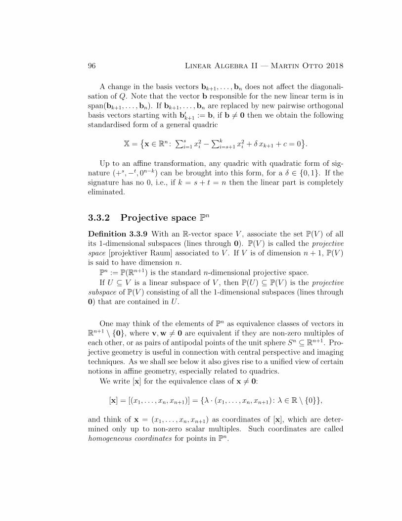
96 Linear Algebra II — Martin Otto 2018
A change in the basis vectors bk+1, . . . ,bn does not affect the diagonali-sation of Q. Note that the vector b responsible for the new linear term is inspan(bk+1, . . . ,bn). If bk+1, . . . ,bn are replaced by new pairwise orthogonalbasis vectors starting with b′k+1 := b, if b 6= 0 then we obtain the followingstandardised form of a general quadric
X ={x ∈ Rn :
∑si=1 x
2i −
∑ki=s+1 x
2i + δ xk+1 + c = 0
}.
Up to an affine transformation, any quadric with quadratic form of sig-nature (+s,−t, 0n−k) can be brought into this form, for a δ ∈ {0, 1}. If thesignature has no 0, i.e., if k = s + t = n then the linear part is completelyeliminated.
3.3.2 Projective space Pn
Definition 3.3.9 With an R-vector space V , associate the set P(V ) of allits 1-dimensional subspaces (lines through 0). P(V ) is called the projectivespace [projektiver Raum] associated to V . If V is of dimension n + 1, P(V )is said to have dimension n.
Pn := P(Rn+1) is the standard n-dimensional projective space.
If U ⊆ V is a linear subspace of V , then P(U) ⊆ P(V ) is the projectivesubspace of P(V ) consisting of all the 1-dimensional subspaces (lines through0) that are contained in U .
One may think of the elements of Pn as equivalence classes of vectors inRn+1 \ {0}, where v,w 6= 0 are equivalent if they are non-zero multiples ofeach other, or as pairs of antipodal points of the unit sphere Sn ⊆ Rn+1. Pro-jective geometry is useful in connection with central perspective and imagingtechniques. As we shall see below it also gives rise to a unified view of certainnotions in affine geometry, especially related to quadrics.
We write [x] for the equivalence class of x 6= 0:
[x] = [(x1, . . . , xn, xn+1)] = {λ · (x1, . . . , xn, xn+1) : λ ∈ R \ {0}},
and think of x = (x1, . . . , xn, xn+1) as coordinates of [x], which are deter-mined only up to non-zero scalar multiples. Such coordinates are calledhomogeneous coordinates for points in Pn.
LA II — Martin Otto 2018 97
en+1
◦
[v]
[u]
A
U•
◦
0
OO
For xn+1 6= 0, [x] possesses a unique representative with xn+1 = 1 in theaffine hyperplane
A = {(x′, 1) : x′ ∈ Rn} ⊆ Rn+1.
The remaining points in Pn correspond to lines through 0 that do notintersect A (parallel to A), or inside the linear subspace U corresponding toA. These points form a projective subspace P(U) ⊆ Pn which is isomorphic toPn−1 = P(Rn) if we identify U with Rn according to U = {(x′, 0) : x′ ∈ Rn}.
The projective space Pn = P(Rn+1) may thus be visualised as the disjointunion of the n-dimensional affine hyperplane A and a “projective hyperplaneat infinity” [unendlich ferne Ebene]. In the case of the projective planeP2 = P(R3), this corresponds to its representation as the disjoint union ofan affine plane and a “line at infinity .” [Just like any other 1-dimensionalprojective subspace, the line at infinity has the topological type of the circleS1, rather than that of a real line.]
Quadrics, affine and projective
A general quadric over Rn+1, with linear and constant terms, does not de-fine a subset of Pn in a natural way, because the defining equation is nothomogeneous. It therefore does not in general define a set of lines in Rn+1,or of points in Pn. More generally, a system of equations over Rn+1 definesa subset in projective space, if each equation is homogeneous in the sense ofhaving the same degree in the coefficients xi in all terms. For a quadric in
98 Linear Algebra II — Martin Otto 2018
Rn+1 to define a subset of Pn, its linear and constant terms must be 0. Wetherefore consider quadrics of the form
X = {x ∈ Rn+1 : Q(x) = 0},
which we take to define the projective set of points
P(X) = {[x] ∈ Pn : x ∈ X \ {0}} ⊆ Pn.
A general quadric, with linear and constant terms over Rn, though, canalways be extended to a homogeneous quadric over Rn+1. We simply usethe extra coordinate xn+1 to pad all terms that are of sub-quadratic degree.From the general quadric
X ={x ∈ Rn :
∑si=1 x
2i −
∑ki=s+1 x
2i + δ xk+1 + c = 0
}⊆ Rn
we pass to the homogeneous, projective quadric
X :={
(x, xn+1) ∈ Rn+1 :∑s
i=1 x2i −
∑ki=s+1 x
2i + δ xk+1xn+1 + cx2n+1 = 0
}in Rn+1, which defines a subset of Pn in terms of homogeneous coordinates.
The effect of this is that the intersection of the new quadric in Rn+1 withthe affine hyperplane A defined by xn+1 = 1, exactly corresponds to the given(inhomogeneous) quadric:
X = X ∩ A.General quadrics are thus seen to be the affine parts of projective quadrics.
Conic sections
Returning to the general quadrics in two-dimensional (projective and affine)planes, we are thus led to analyse them in terms of the projective quadrics,or the homogeneous quadrics in R3 which are of the form
Q(x, y, z) = 0.
There are only just a few types, depending on the signature of the quadraticform: (+,+,+), (+,+,−), (+,+, 0), (+,−, 0), (+, 0, 0) and (0, 0, 0). We mayresort to our classification above, looking just at the cases c = 0.
For non-degenerate Q, the only non-trivial case to be considered is thatof signature (+,+,−). Up to linear transformations as detailed above,
X = {(x, y, z) : x2 + y2 = z2}
LA II — Martin Otto 2018 99
defines a cone, which is clearly a union of lines through 0 in R3. All non-degenerate general quadrics in the affine plane are thus seen to be conicsections [Kegelschnitte] in the sense of being (linearly equivalent to) theintersections of the image of the standard cone X under some linear trans-formation with the affine hyperplane A = {(x, y, z) : z = 1} ⊆ R3.
The only distinguishing feature between the different affine incarnationsis determined by where the projective line at infinity intersects X \ {0}. Welet U be the x-y-plane, parallel to A; P(U) the line at infinity. There are thefollowing cases:
• no intersection: P(U) ∩ X = ∅. U cuts the cone in the origin only.The affine part is an ellipse (or, up to affine transformations within A,equivalent to the unit circle S1).
• one point of intersection: |P(U) ∩ X| = 1. U cuts the cone in preciselyone line on its mantle. The affine part is a parabola (or, up to affineequivalence the standard parabola y = x2).
• two points of intersection: |P(U)∩X| = 2. U cuts the cone in preciselytwo lines on its mantle. The affine part is a hyperbola (or, up to affineequivalence the standard hyperbola x+ y = 1
x−y ).
Remark 3.3.10 In a similar way, and one dimension up, qualitatively differ-ent three-dimensional affine quadrics as for instance the single-sheet hyper-boloid and its relative, the saddle surface {(x, y, z) : x2−y2 = z} are seen to bedifferent affine sections of the projective quadric X =
{[x] : x4x3− x1x2 = 0}
of signature (+,+,−,−). The three other prominent three-dimensional affinequadrics, the two-sheet hyperboloid, the ellipsoid and the paraboloid are alsojust distinct affine views of the same projective point set, viz., of the projec-tive quadric with signature (+,+,+,−).
Exercise 3.3.2 Determine the projective hull X of the above-mentionedthree-dimensional affine quadrics and determine the underlying signatures.In order to demonstrate the distinctions between the two mentioned families– single-sheet hyperboloids and saddle surfaces on one hand, and two-sheethyperboloids, the ellipsoids and paraboloids on the other – show that theformer are generated by families of affine lines, while the latter do not con-tain any lines. It follows that members of the second family cannot occuras projective images of members from the first family (why?). Within eachfamily, describe the different affine views in terms of different choices for theplane at infinity.
100 Linear Algebra II — Martin Otto 2018
3.3.3 Appendix: an example from classical mechanics
Consider the motion of a rigid body, whose centre of gravity is at rest, instandard euclidean 3-space (R3, 〈., .〉). We choose a fixed frame of referencewith the null vector at the body’s centre of mass, and choose an orthonormalbasis B = (b1,b2,b3) as a system of coordinates for points in space. Then thecurrent position of the rigid body at time t can be described by the isometryϕt ∈ SO(3) that transforms its original position (the frame B = (b1,b2b3))at time 0 into its current position (the frame B(t) = (b1(t),b2(t),b3(t)) ascarried along with the motion of the rigid body). In other words, the isometryϕt transforms the fixed frame of reference B = (b1,b2,b3) = B(0) of the ex-ternal observer into the moving frame of reference B(t) = (b1(t),b2(t),b3(t))that an inhabitant of the rigid body would regard as stationary. Note that[[ϕt]]
BB has column vectors [[b1(t)]]B, [[b2(t)]]B, [[b3(t)]]B and is therefore orthog-
onal, i.e., an isometry.The momentary velocities of points in the rigid body (relative to the
external frame) are obtained as time derivatives as follows. If x is a fixedlocation in B(0) (a particle of the rigid body), then this point moves alongthe trajectory r(t) = ϕt(x) and its momentary velocity at time t is
r(t) = ϕt(x) = ϕt(ϕ−1t (r(t))) =
(ϕt ◦ ϕ−1t
)(r(t)),
where ϕt is the time derivative of the curve t 7→ ϕt in SO(3) at time t.Differential calculus and linear algebra show that the momentary motion attime t as seen from the external observer can be described as a momentaryrotation about a momentary axis of rotation as follows.
The idea is to describe this momentary rotation (and, depending on it,the velocities of particles in the body) in terms of an angular velocity vectorω(t) such that span(ω(t)) is the current axis of rotation, and the length ω(t)of ω(t) is the scalar angular velocity.1
The current axis of rotation, span(ω(t)), is geometrically determined as
span(ω(t)) = ker(ϕt ◦ ϕ−1t ) = ϕt(ker(ϕt))
as the following simple analysis shows. Applying the derivative w.r.t. thetime parameter t to the constant function id = ϕt ◦ ϕ−1t = ϕt ◦ (ϕt)
+, we
1The absolute value of the scalar angular velocity is the time derivative of the angle inpolar coordinates; its sign need to match the orientation of ω(t).
LA II — Martin Otto 2018 101
obtain (by a component-wise application of the product rule to coefficients inmatrix representations, and using the fact that the time derivative commuteswith transposition)
0 = (id) = ϕt ◦ ϕ+t + ϕt ◦ (ϕt)
+ = ϕt ◦ ϕ−1t + ϕt ◦ (ϕt)+.
It follows that ϕt◦ϕ−1t is an anti-symmetric (skew-symmetric) endomorphismof (R3, 〈., .〉):
(ϕt ◦ ϕ−1t )+ = −(ϕt ◦ (ϕt)+)+ = −ϕt ◦ ϕ+
t = −ϕt ◦ ϕ−1t .
This implies that ϕt ◦ ϕ−1t is either null or has a 1-dimensional kernel,which then uniquely determines the momentary axis of rotation span(ω(t)).Moreover, the orthogonal complement of span(ω(t)) is also an invariant sub-space of ϕt◦ϕ−1t and, by anti-symmetry, ϕt◦ϕ−1t operates on (span(ω(t)))⊥ asa rotation through π/2 and a rescaling, which determines the scalar angularvelocity ω(t). W.r.t. to the vector product in R3, we find
(ϕt ◦ ϕ−1t )(r(t)) = r(t) = ϕt(x) = ω(t)× r = ω(t)× ϕt(x).
In the absence of external forces, the laws of classical mechanics put twoconstraints on the dynamics of this motion: conservation of kinetic energyK(t) and of angular momentum L(t). Therefore the dependence of thesequantities on ϕt and ω(t) governs the equations of motion.
The contribution to the angular momentum of an individual unit massparticle at a fixed position x in the rigid body (and thus at position r(t) =ϕt(x) relative to B(0)) is
r(t)× r(t) = ϕt(x)× (ω(t)× ϕ(x)) = ϕt(x× (ϕ−1t (ω(t))× x)
),
which is linear in ω(t). Our insights into change of basis transformationsshow that the time-independent linear map
I : ϕ−1t (ω(t)) 7−→ ϕ−1t (L(t))
represents the map ω(t) 7−→ L(t) in terms of the moving frame of referenceB(t). It is called the moment of inertia and only depends on the distributionof mass within the rigid body. Moreover, this endomorphism is self-adjointor symmetric w.r.t. the standard scalar product.
102 Linear Algebra II — Martin Otto 2018
Another map, ω(t) 7−→ K(t), similarly expresses the kinetic energy interms of just ϕ−1t (ω(t)) and the static moment of inertia I. It has the formatof a quadratic form:
ω(t) 7−→ K(t) = 〈ω(t),L(t)〉 = 〈ϕ−1t (ω(t)), ϕ−1t (L(t))〉= 〈ϕ−1t (ω(t)), I(ϕ−1t (ω(t)))〉,
which is time-independent w.r.t. to the moving frame B(t). As the last lineshows, in terms of the moving frame of reference B(t), K corresponds to thesymmetric bilinear form induced by I,
σI = 〈u,v〉I : (u,v) 7−→ 〈u, Iv〉.
The moment of inertia, therefore appears in the role of a self-adjointendomorphism (mapping angular velocity to angular momentum) as wellas in the role of a symmetric bilinear form (with quadratic form mappingangular momentum to kinetic energy), in exactly the manner discussed insection 3.2.1.
As our general analysis showed, endomorphisms of Rn that are self-adjoint(symmetric) can always be diagonalised w.r.t. an orthonormal basis – equiv-alently, the associated symmetric bilinear and the induced quadratic formscan be diagonalised w.r.t. pairwise orthogonal principal axes. In our case thismeans that I admits a diagonal representation
[[I]]BB =
λ1 0 00 λ2 00 0 λ3
= [[σI ]]B
w.r.t. the right choice of orthonormal basis B = (b1,b2,b3) = B(0) (whichis carried along with ϕt to produce B(t), in which I is statically representedin this diagonal form). The eigenvalues λi are determined as the zeroesof the characteristic polynomial pI = det(I − λid), and in our case are allpositive: for physical reasons, the symmetric bilinear form σI is positivedefinite. If the λi are pairwise distinct, then the three distinguished axesspanned by corresponding eigenvectors are uniquely determined and definethree pairwise orthogonal axes (static only in the moving frame of referenceB(t), fixed relative to the rigid body). These are the principal axes of inertiaof the rigid body.
The current axis of rotation span(ω) is aligned with the angular momen-tum L if, and only if, ϕ−1t (ω) is an eigenvector of I. So, in the generic case
LA II — Martin Otto 2018 103
with three distinct eigenvalues, there are just three admissible axes of rotationthat can be static relative to the rigid body: if ϕ−1t (ω) is not an eigenvectorof I, then conservation of angular momentum implies that L rather than ωis constant. Combining this with the constraint imposed by conservation ofkinetic energy, one can see that among the three axes that are admissibleas stationary axes of rotation, only the ones with the extremal eigenvaluesconstitute a stable equilibrium. The axis of the intermediate eigenvalue cantilt away in two independent directions without violating either conservationof energy or angular momentum.
The analysis shows that the two conservation conditions constrain ϕ−1t (ω)(i.e., ω w.r.t. the moving frame) to an ellipsoid (for constant K(t)) and toa sphere (for constant L(t) in the external frame). In the distinguishedorthonormal basis B = (b1,b2,b3) that diagonalises I and for ϕ−1t (ω) =∑
i ωibi, the condition
K = σI(ϕ−1t (ω), ϕ−1t (ω)) = 〈ϕ−1t (ω), Iϕ−1t (ω)〉 =
∑i λiω
2i = c
defines an ellipsoid with principal axes spanned by the basis vectors bi. Asphere that meets a concentric ellipsoid in the end points of one of its principalaxes locally has the following intersection pattern with the ellipsoid:
(i) a single point (stable) in the case of the longest principal axis (minimaleigenvalue): the whole ellipsoid lies inside the sphere;
(ii) a single point (stable) in the case of the shortest principal axis (maximaleigenvalue): the whole sphere lies inside the ellipsoid;
(iii) two crossing curves of intersection (unstable) in the case of the inter-mediate axis: the ellipsoid is partly inside, partly outside the sphere.
These phenomena are easily displayed in simple experiments.

104 Linear Algebra II — Martin Otto 2018
Index
adjoint (Adjungierte), 57, 75, 76adjoint map (adjungierte Abbildung),
75, 76adjoint matrix (adjungierte Matrix ), 57affine hyperplane (affine Hyperebene),
97algebraic multiplicity (algebraische
Multiplizitat), 21angle (Winkel), 49, 53
bilinear form (Bilinearform), 51, 55,81, 82, 84
block decomposition (Blockzerlegung),14, 37–39, 45, 72, 73
Cauchy–Schwarz (Cauchy–Schwarz ), 59Cayley–Hamilton (Cayley–Hamilton),
30characteristic polynomial
(charakteristisches Polynom),13, 30, 33, 34
column vector (Spaltenvektor), 49cone (Kegel), 93conic section (Kegelschnitt), 99constant polynomial (konstantes
Polynom), 17cylinder (Zylinder), 94
degree (Grad), 16diagonal matrix (Diagonalmatrix ), 15diagonalisation (Diagonalisierung), 15,
34, 35, 79, 80, 82, 84–87, 91divisibility (Teilbarkeit), 20
division with remainder (Division mitRest), 20
eigenspace (Eigenraum), 12eigenvalue (Eigenwert), 7, 11eigenvalue problem
(Eigenwertproblem), 12eigenvector (Eigenvektor), 7, 11ellipsoid (Ellipsoid), 93euclidean space (euklidischer Raum),
49, 52
fundamental theorem of algebra(Fundamentalsatz derAlgebra), 24
geometric multiplicity (geometrischeMultiplizitat), 12
Gram–Schmidt (Gram–Schmidt), 65greatest common divisor (großter
gemeinsamer Teiler), 23
hermitian (hermitesch), 54, 57hermitian matrix (hermitesche
Matrix ), 76, 77, 83homogeneous coordinates (homogene
Koordinaten), 96hyperbola (Hyperbel), 91, 93, 94, 99hyperboloid (Hyperboloid), 94hyperplane at infinity (unendlich ferne
Hyperebene), 97
ideal (Ideal), 22integral domain (Integritatsbereich), 19
105
106 Linear Algebra II — Martin Otto 2018
invariant subspace (invarianterUnterraum), 7, 14
isometric (isometrisch), 49
isometry (Isometrie), 49, 62, 73
Jordan normal form (JordanNormalform), 36, 45
leading coefficient (Leitkoeffizient), 16
length (Lange, Betrag), 49, 52, 55
line at infinity (unendlich ferneGerade), 97
linear factor (Linearfaktor), 21
linear polynomial (lineares Polynom),17
matrix representation(Matrixdarstellung), 7, 10, 81,82
metric (Metrik), 59, 60
metric structure (metrische Struktur),49
minimal polynomial(Minimalpolynom), 30, 32–34
multiplicity (Multiplizitat), 12, 21
negatively oriented (negativ orientiert),74
non-degenerate (nicht ausgeartet), 83
non-degenerate bilinear form(nicht-ausgearteteBilinearform), 84
norm (Norm), 52, 55
normal (normal), 78
normal map (normale Abbildung), 78,80
normal matrix (normale Matrix ), 78–80
normalisation (Normalisierung), 52
null polynomial (Nullpolynom), 16
orientation (Orientierung), 74
orthognal matrix (orthogonale Matrix ),87
orthogonal (orthogonal), 53, 55, 66, 71orthogonal complement (orthogonales
Komplement), 66orthogonal group (orthogonale
Gruppe), 70orthogonal map (orthogonale
Abbildung), 70orthogonal projection
(Orthogonalprojektion), 68, 75orthonormal basis (Orthonormalbasis),
64orthonormal system
(Orthonormalsystem), 64
parabola (Parabel), 99polarisation (Polarisation), 61polynomial (Polynom), 16polynomial function
(Polynomfunktion), 17positive definite (positiv definit), 51,
54, 88positively oriented (positiv orientiert),
74power (Potenz ), 16principal axes (Hauptachsen), 84, 86principal ideal (Hauptideal), 22principal minor (Hauptminor), 88projective space (projektiver Raum), 96projective subspace (projektiver
Unterraum), 96
quadratic form (quadratische Form),81, 89, 90
quadratic polynomial (quadratischesPolynom), 17
quadric (Quadrik), 89, 92
regular matrix (regulare Matrix ), 84relatively prime (teilerfremd), 23, 35
LA II — Martin Otto 2018 107
remainder (Rest), 20ring of polynomials (Polynomring), 18root (Wurzel), 21row vector (Zeilenvektor), 49
scalar product (Skalarprodukt), 49, 51,52, 54
self-adjoint map (selbstadjungierteAbbildung), 75, 76, 83, 84
self-adjoint matrix (selbstadjungierteMatrix ), 57, 76, 83
semi-bilinear (semi-bilinear), 54sesquilinear (sesquilinear), 54signature (Signatur), 86, 92simultaneous diagonalisation
(simultane Diagonalisierung),82, 84–87, 91
single-sheet hyperboloid (einschaligesHyperboloid), 94
special orthogonal group (spezielleorthogonale Gruppe), 74
standard scalar product (StandardSkalarprodukt), 51, 54
Sylvester (Sylvester), 85symmetric bilinear form (symmetrische
Bilinearform), 51, 83, 84,88–90
symmetric map (symmetrischeAbbildung), 75
symmetric matrix (symmetrischeMatrix ), 76, 77, 83, 87
transpose (Transponierte), 50two-sheet hyperboloid (zweischaliges
Hyperboloid), 94
unit vector (Einheitsvektor), 52, 55unitary group (unitare Gruppe), 70unitary map (unitare Abbildung), 70unitary matrix (unitare Matrix ), 71, 80unitary space (unitarer Raum), 49, 54
upper triangle matrix (obereDreiecksmatrix ), 25, 33
zero of polynomial (Nullstelle), 21
Index (deutsch)
Adjungierte (adjoint), 57, 75, 76adjungierte Abbildung (adjoint map),
75, 76adjungierte Matrix (adjoint matrix ), 57affine Hyperebene (affine hyperplane),
97algebraische Multiplizitat (algebraic
multiplicity), 21
Bilinearform (bilinear form), 51, 55, 81,82, 84
Blockzerlegung (block decomposition),14, 37–39, 45, 72, 73
Cauchy–Schwarz (Cauchy–Schwarz ), 59Cayley–Hamilton (Cayley–Hamilton),
30charakteristisches Polynom
(characteristic polynomial), 13,30, 33, 34
Diagonalisierung (diagonalisation), 15,34, 35, 79, 80, 82, 84–87, 91
Diagonalmatrix (diagonal matrix ), 15Division mit Rest (division with
remainder), 20
Eigenraum (eigenspace), 12Eigenvektor (eigenvector), 7, 11Eigenwert (eigenvalue), 7, 11Eigenwertproblem (eigenvalue
problem), 12Einheitsvektor (unit vector), 52, 55
einschaliges Hyperboloid (single-sheethyperboloid), 94
Ellipsoid (ellipsoid), 93euklidischer Raum (euclidean space),
49, 52
Fundamentalsatz der Algebra(fundamental theorem ofalgebra), 24
geometrische Multiplizitat (geometricmultiplicity), 12
großter gemeinsamer Teiler (greatestcommon divisor), 23
Grad (degree), 16Gram–Schmidt (Gram–Schmidt), 65
Hauptachsen (principal axes), 84, 86Hauptideal (principal ideal), 22Hauptminor (principal minor), 88hermitesch (hermitian), 54, 57hermitesche Matrix (hermitian
matrix ), 76, 77, 83homogene Koordinaten (homogeneous
coordinates), 96Hyperbel (hyperbola), 91, 93, 94, 99Hyperboloid (hyperboloid), 94
Ideal (ideal), 22Integritatsbereich (integral domain), 19invarianter Unterraum (invariant
subspace), 7, 14Isometrie (isometry), 49, 62, 73
108
LA II — Martin Otto 2018 109
isometrisch (isometric), 49
Jordan Normalform (Jordan normalform), 36, 45
Kegel (cone), 93Kegelschnitt (conic section), 99konstantes Polynom (constant
polynomial), 17
Lange, Betrag (length), 49, 52, 55Leitkoeffizient (leading coefficient), 16lineares Polynom (linear polynomial),
17Linearfaktor (linear factor), 21
Matrixdarstellung (matrixrepresentation), 7, 10, 81, 82
Metrik (metric), 59, 60metrische Struktur (metric structure),
49Minimalpolynom (minimal
polynomial), 30, 32–34Multiplizitat (multiplicity), 12, 21
negativ orientiert (negatively oriented),74
nicht ausgeartet (non-degenerate), 83nicht-ausgeartete Bilinearform
(non-degenerate bilinear form),84
Norm (norm), 52, 55normal (normal), 78normale Abbildung (normal map), 78,
80normale Matrix (normal matrix ), 78–80Normalisierung (normalisation), 52Nullpolynom (null polynomial), 16Nullstelle (zero of polynomial), 21
obere Dreiecksmatrix (upper trianglematrix ), 25, 33
Orientierung (orientation), 74
orthogonal (orthogonal), 53, 55, 66, 71
orthogonale Abbildung (orthogonalmap), 70
orthogonale Gruppe (orthogonalgroup), 70
orthogonale Matrix (orthognal matrix ),87
orthogonales Komplement (orthogonalcomplement), 66
Orthogonalprojektion (orthogonalprojection), 68, 75
Orthonormalbasis (orthonormal basis),64
Orthonormalsystem (orthonormalsystem), 64
Parabel (parabola), 99
Polarisation (polarisation), 61
Polynom (polynomial), 16
Polynomfunktion (polynomialfunction), 17
Polynomring (ring of polynomials), 18
positiv definit (positive definite), 51,54, 88
positiv orientiert (positively oriented),74
Potenz (power), 16
projektiver Raum (projective space), 96
projektiver Unterraum (projectivesubspace), 96
quadratische Form (quadratic form),81, 89, 90
quadratisches Polynom (quadraticpolynomial), 17
Quadrik (quadric), 89, 92
regulare Matrix (regular matrix ), 84
Rest (remainder), 20
110 Linear Algebra II — Martin Otto 2018
selbstadjungierte Abbildung(self-adjoint map), 75, 76, 83,84
selbstadjungierte Matrix (self-adjointmatrix ), 57, 76, 83
semi-bilinear (semi-bilinear), 54sesquilinear (sesquilinear), 54Signatur (signature), 86, 92simultane Diagonalisierung
(simultaneous diagonalisation),82, 84–87, 91
Skalarprodukt (scalar product), 49, 51,52, 54
Spaltenvektor (column vector), 49spezielle orthogonale Gruppe (special
orthogonal group), 74Standard Skalarprodukt (standard
scalar product), 51, 54Sylvester (Sylvester), 85symmetrische Abbildung (symmetric
map), 75symmetrische Bilinearform (symmetric
bilinear form), 51, 83, 84,88–90
symmetrische Matrix (symmetricmatrix ), 76, 77, 83, 87
Teilbarkeit (divisibility), 20teilerfremd (relatively prime), 23, 35Transponierte (transpose), 50
unendlich ferne Gerade (line atinfinity), 97
unendlich ferne Hyperebene(hyperplane at infinity), 97
unitare Abbildung (unitary map), 70unitare Gruppe (unitary group), 70unitare Matrix (unitary matrix ), 71, 80unitarer Raum (unitary space), 49, 54
Winkel (angle), 49, 53
Wurzel (root), 21
Zeilenvektor (row vector), 49zweischaliges Hyperboloid (two-sheet
hyperboloid), 94Zylinder (cylinder), 94