lending relationships in the interbank market
TRANSCRIPT
Lending Relationships in the Interbank Market∗
João F. Cocco†
Francisco J Gomes‡
Nuno C. Martins§
July 2005
∗We would like to thank Viral Acharya, Andrea Buraschi, Jennifer Conrad, Francesca Cornelli, Denis
Gromb, Michel Habib, Philipp Hartmann, Narayan Naik, Jose Peydro-Alcayde, Mitchell Petersen, Maximiano
Pinheiro, Raghuram Rajan, Rafael Repullo, Henri Servaes and seminar participants at the Bank of England,
Banco de Portugal, Cass Business School, European Central Bank, London Business School, London School
of Economics, the 2002 European Winter Meetings of the Econometric Society, the 2004 American Finance
Association meetings, and the 2005 Conference on Competition, Stability, and Integration in European Bank-
ing for helpful comments and suggestions. We are especially grateful to an anonymous referee for detailed and
constructive comments. The analysis, opinions and findings of this paper represent the views of the authors,
they are not necessarily those of the Banco de Portugal.†London Business School, Regent’s Park, London NW1 4SA, UK, and CEPR. Email [email protected].‡London Business School, Regent’s Park, London NW1 4SA, UK, and CEPR. Email [email protected]§Universidade Nova de Lisboa and Banco de Portugal, Av. Almirante Reis, 71, 1150-012 Lisboa, Portugal.
E-mail [email protected]
1

Abstract
We use a unique dataset to study lending relationships in the interbank market. We explic-
itly control for the endogeneity of lending relationships, and find that borrowers pay a lower
interest rate on loans from banks with whom they have a stronger relationship. Moreoever,
we find that smaller banks, banks with lower return on assets, banks with a higher propor-
tion of non-performing loans, and banks subject to more volatile liquidity shocks rely more
on lending relationships. Finally, we find evidence that smaller banks with limited access to
international markets tend to rely on lending relationships when borrowing in the domestic
interbank market. This provides evidence that banks rely on lending relationships to overcome
monitoring and default risk problems, and for insurance purposes.
1 Introduction
Many interactions between economic agents are of a frequent and repeated nature. In such
a setting agents may establish relationships, and equilibrium outcomes may be very different
from those that arise in a spot market. One important setting in which there are frequent
and repeated interactions between agents is the interbank market. Our paper studies the role
of lending relationships in this market.
Understanding lending behavior and price formation in the interbank market is important
for banks who use it to engage in unsecured borrowing and lending of funds. It is also
important for monetary authorities, since the interbank market lies at the heart of monetary
policy. Moreover, it is in this market that the overnight rate is determined, which is the
shortest-term market interest rate, and as such it has a crucial role in term structure models.
The interbank market is fragmented in nature. For direct loans, which account for most
of the lending volume, the loan’s amount and interest rate are agreed on a one-to-one basis
between borrower and lender. Other banks do not have access to the same terms, and do
not even know that the loan took place. When quotes are posted on screens, they are merely
indicative. This market structure allows banks to establish lending relationships.1
But which economic purpose do lending relationships in interbank markets serve? The
literature has focused on the function of these markets has distributors of liquidity. In the
model of Ho and Saunders (1985), the reserve position of each bank is affected by stochastic
deposits and withdrawals by customers. As a result banks trade in order to meet their reserve
requirements. Similarly, in the model of Bhattacharya and Gale (1987) banks borrow and
lend funds in order to insure against intertemporal liquidity shocks. In the model of Allen and
Gale (2000) liquidity shocks arise from uncertainty in the timing of depositors’ consumption.
Banks hold deposits with banks in other regions to insure against liquidity shocks in their
own region. Finally, in the model of Freixas, Parigi and Rochet (2000) the uncertainty and
1The issue of price formation and the properties of prices in centralized versus fragmented markets has
been the subject of much research (see for example Wolinsky, 1990, Biais, 1993, and O’Hara, 1995).
1
interbank lending arise from consumers’ uncertainty about where to consume. A common
feature to these (and other) models of the interbank market are liquidity shocks, that give
rise to borrowing and lending. Lending relationships may provide insurance against liquidity
shocks.
Another important strand of the literature focuses on the role of peer monitoring in inter-
bank markets (see the models of Rochet and Tirole, 1996, Freixas and Holthausen, 2005, and
the empirical analysis in Furfine, 2001). Peer monitoring is important because of the large
and unsecured nature of the loans. Thus, lending relationships may help overcome agency
problems.
In addition to focusing on lending relationships in the interbank market, the main novelty
of our analysis is that we recognize that the decision of whether to rely on lending relationships
is an endogenous choice, and our econometric approach treats it as such. For this reason we
are able to provide new insights into the determinants of lending relationships.
We use a unique dataset that contains information on all direct loans that took place in
the Portuguese interbank market between January 1997 and August 2001. The Portuguese
interbank market is in many respects typical and, although smaller, it is organized similarly
to the US Fed Funds market. Our dataset identifies the date, interest rate, amount, maturity,
lender and borrower of each loan. Thus, we can track loans between each and every pair
of banks, and with other banks over time. Using this information, we construct dynamic
measures of relationships based on the intensity of pair-wise lending activity. Our dataset
also includes daily information on each bank’s reserve deposits, and quarterly information
on banks’ balance sheet variables including total assets, return on assets and proportion of
non-performing loans.
We first investigate the link between the loan interest rate and relationship measures. To
address the endogeneity issue we estimate instrumental variables regressions, in which we
explore the time-series dimension of our dataset by using lagged relationship measures as
instruments. Obviously such instruments are not available in cross-sectional data, which is
typically used in the existing literature on lending relationships. Importantly, we find that
2

borrowers pay a lower interest rate on loans from banks with whom they have a stronger
lending relationship. We also find that once we control for the endogeneity of lending rela-
tionships, several other explanatory variables are no longer important for explaining the loan
interest rate.
The instrumental variables regressions allow us to identify the causal link between rela-
tionship measures and the loan interest rate, but they do not explain the determinants of
lending relationships. To do so we estimate a seemingly unrelated regressions system of equa-
tions, with the amount lent, the interest rate, and the relationship measures for lender and
borrower as dependent variables. This allows us to simultaneously study the determinants of
loan pricing, loan amount, and of lending relationships.
Our main findings are as follows. First, we find that borrowers with lower return on
assets and with a higher proportion of non-performing loans are more likely to rely on lending
relationships. These results provide empirical support for an explanation of these relationships
based on default risk and monitoring.
We use the information on each bank’s reserve deposits to construct a measure of liquidity
shocks which is equal to the daily change in these deposits. We find that borrowers with
more volatile liquidity shocks are more likely to rely on lending relationships. They tend to
do so with lenders who have less volatile liquidity shocks, and also with whom they have
less correlated shocks. In addition, borrowers are more likely to rely on lending relationships
when they experience a larger imbalance in their reserve deposits. This provides evidence that
banks rely on lending relationships for insurance.
We find that small borrowers are more likely to establish relationships and that they tend
to choose larger banks as their preferred lenders. Furthermore, large banks tend to be net
borrowers, while small banks tend to be net lenders in the market. Interestingly, this pattern
of trade is also a distinctive feature of the US Fed Funds market (Furfine, 1999, Ho and
Saunders, 1985).
Finally, we investigate how banks’ ability to access international markets affect the nature
of lending relationships in the domestic interbank market. We find that small banks and banks
3
with a higher proportion of non-performing loans tend to have limited access to international
markets, and that they tend concentrate their borrowing when borrowing funds in the domestic
interbank market. This result may be due to peer monitoring across borders being less efficient
than at the domestic level, as in the model of Freixas and Holthausen (2005).
Our results for the pricing or interbank loans are consistent with those of Furfine (2001)
for the Fed Funds market. We find that, controlling for the degree of lending relationship and
holding the size of the counterparty fixed, larger banks borrow and lend at more favorable
terms. Banks with higher return on assets lend at higher interest rates. This is consistent
with these banks having a higher opportunity cost of lending funds in the interbank market,
and requiring a higher interest rate to do so. Borrowers with a higher proportion of non-
performing loans tend to pay higher interest rates. Again controlling for the degree of lending
relationship, we find that more profitable banks lend less, and banks with a higher proportion
of non-performing loans lend more and borrow less. Thus banks that have better investment
opportunities tend to be net borrowers.
There is a large literature on lending relationships that focuses on bank-firm relationships.
It has found evidence that lending relationships help overcome constraints that arise from
monitoring and default risk between borrower and lender of funds,2 and allow banks to provide
insurance to firms in the form of interest-rate smoothing.3 Thus this literature focuses on long-
term relationships between banks and firms, by which banks acquire inside knowledge about
firm characteristics or the project that is being financed. Although somewhat related, it is
important to note that these relationships are of a different nature than the ones that we
study in our paper, which are transaction based.
The paper proceeds as follows. Section 2 describes the data, our relationship metrics and
reports some summary statistics. Section 3 studies the pricing of interbank loans. Section 4
2See Berger and Udell (1995), Lummer and McConnell (1989), Petersen and Rajan (1994), Slovin, Sushka,
and Poloncheck (1993).3See Berger and Udell (1992), Berlin and Mester (1999), Petersen and Rajan (1995), or Ongena and Smith
(2000) for a survey of the literature on bank lending relationships.
4

investigates the determinants of lending relationships. Section 5 presents additional evidence
on the determinants of lending relationships, that allows us to be more precise with respect
to their nature. Section 6 reports some robustness checks. Section 7 concludes.
2 The Data
2.1 Description
We combine information from three different datasets, which we have obtained from the Por-
tuguese Central Bank. The first dataset has information on all direct loans in the Portuguese
interbank market from January 1997 to August 2001. The Portuguese interbank market is a
typical interbank market, and although of a smaller size, it functions in a similar way to the
Fed Funds market. Each loan may be either borrower or lender initiated. When a bank wishes
to borrow or lend funds, it approaches another bank, identifies itself, and asks for prices, i.e.
interest rates, for borrowing and lending funds at a given maturity. It is very rare that banks
asking for quotes are turned down, or simply refused funds. But banks do provide different
quotes for different banks that approach them, and it is common practice for banks to shop
around for the best rates.
Our dataset is unique in that it comprises all direct loans, and contains information on
the loan’s date, amount, interest rate, and maturity, as well as the identity of the lender and
the borrower. Being able to identify the lender and borrower for each loan and to observe all
loans over a long period of time is crucial for our study of lending relationships. Even though
interbank loans are privately negotiated, they must be reported to the central bank, who is
responsible for their settlement, by debiting and crediting the reserve accounts of borrowers
and lenders.
We restrict our analysis to overnight loans, i.e. loans maturing on the next business day.
We do so because the interbank market is mainly a market for short-term borrowing and
lending of funds: during our sample period there were 44, 768 overnight loans accounting for
5
over 75 percent of the total amount lent (casual evidence suggests that this is a common
feature in most interbank markets). Even though credit risk for loans of overnight maturity
may be small, it is important to note that these are large and uncollaterized loans, with an
average loan amount of roughly twelve million euros. Therefore we expect that even small
differences across banks in credit risk are reflected on the loan interest rate.
The second dataset provides daily information on the balance in banks’ reserve accounts. It
allows us to study how banks’ reserve position affects their behavior in the interbank market.
The third dataset contains quarterly information on bank characteristics, including total
assets, financial and profitability ratios and credit risk variables. This dataset also allows us
to determine whether the bank belongs to a banking group, defined in terms of control of the
institution. We exclude loans between banks belonging to the same group, which leaves us
with a total of 37, 701 overnight loans.
2.2 Measuring Lending Relationships
We measure lending relationships by the intensity of lending activity between banks. We use
two alternative measures. Our first measure is based on how concentrated the banks’ lending
and borrowing activity is. More precisely, for every given lender (L) and every borrower (B),
we compute a lender preference index (LPI), equal to the ratio of total funds that L has
lent to B during a given year/quarter, over the total amount of funds that L has lent in the
interbank market during that same year/quarter.4 Let F j−→ki denote the amount lent by bank
j to bank k on loan i then:
LPI%L,B,q =Xi∈q
FL−→Bi /
Xi∈q
FL−→alli (1)
where q denotes year/quarter. This ratio is more likely to be high if L relies on B more than
on other banks to lend funds in the market.4We discuss our choice of time period in detail below.
6
Similarly, we compute a borrower preference index (BPI) as the ratio of total funds that
B has borrowed from L in a given year/quarter, as a fraction of the total amount of funds
that B has borrowed in the market in that same year/quarter:
BPI%L,B,q =Xi∈q
FL−→Bi /
Xi∈q
F any−→Bi . (2)
Our second measure of lending relationships is simply the (absolute) number of different
banks to which bank L lent funds during year/quarter q, and similarly the number of different
banks from which bank B borrowed funds during year/quarter q:
LPI#L,q = Number of banks to which bank L lent funds in year/quarter q (3)
BPI#B,q = Number of banks from which bank B borrowed funds in year/quarter q (4)
Thus our first measure of lending relationships is a relative measure, while our second
measure is an absolute one. Elsas, Heinemann, and Tyrell (2004) solve a model in which for
some borrowers it is optimal to rely on multiple but asymmetric financing, i.e. borrowing a
large amount from a single bank, and the remaining amount from several other banks. This
asymmetry in financing can not be captured by the absolute number of different lenders.
For this reason we have decided to use both an absolute and a relative measure of lending
relationships. As one might expect, the correlation between these measures is negative. The
correlation between the BPI% and BPI# indices is equal to −0.46, while the correlationbetween the LPI% and LPI# indices is equal to −0.42Figure 1 plots, for a given quarter and for a given borrower, its BPI% indices with different
lenders. The most important lender for this borrower during this quarter is the bank labeled
as lender one, from which it borrowed roughly a quarter of the total funds that it borrowed
during the quarter. This figure illustrates that in our data there are asymmetries in financing,
with some lenders being much more important than others.
As an illustrative example of the time-series dimension of our relationship measures, Figure
2 plots the evolution of the LPI% and BPI% indices for a pair of banks in our sample, L and
7
B. This time-series dimension of our data is important because it will allow us to deal with
the issue of the endogeneity of lending relationships. More precisely, since there is a time-
series dimension in our data we will be able to use lagged relationship measures as (exogenous)
instruments. Figure 2 also illustrates that there is time variation in our relationship measures.
In our regressions the explanatory power comes both from cross-sectional differences across
banks, as well as changes over time in bank characteristics.
We have chosen the calendar quarter to measure lending relationships. To some extent this
choice is arbitrary. A lending relationship should be fairly stable over time, but not immutable
through time. In addition, there is a practical reason to choose the calendar quarter as unit of
analysis, since some of our bank data is quarterly, namely information about the banks’ assets,
profitability and credit risk. In section 6 we show that the results are robust to alternative
ways of measuring relationships.
2.3 Profitability and Credit Risk Variables
One possible motive for lending relationships is that they may help overcome agency problems
that arise from asymmetric information between borrowers and lenders of funds. Rochet and
Tirole (1996) solve a model of the interbank market in which monitoring plays an important
role.5 For this reason we include as explanatory variables total assets, the quarterly return
on assets (ROA), and the proportion of non-performing loans (NPL). The latter is defined as
loans that are past-due for a period exceeding 90 days, over total outstanding credit granted
by the bank. Obviously, the latter includes loans granted to individuals and firms, and not
only to other banks.
5Broecker (1990), Flannery (1996), and Freixas and Holthausen (2005) also solve models of the interbank
market with asymmetric information and credit risk. Freixas and Holthausen (2005) solve such a model in an
international setting, when cross-country information is noisy.
8
2.4 Insurance variables
A second possible reason for banks to establish lending relationships is to obtain insurance
against idiosyncratic liquidity shocks, arising from withdrawals by retail depositors. A bank
may borrow the funds needed to meet unexpectedly large withdrawals from other banks in the
interbank market (see the models of Ho and Saunders, 1985, Bhattacharya and Gale, 1987,
and Freixas, Parigi and Rochet, 2000).
If lending relationships are important for insurance purposes, we might expect banks sub-
ject to more volatile liquidity shocks to rely more on them. To investigate this hypothesis we
construct a measure of volatility of liquidity shocks, equal to the standard deviation of the
daily change in the bank’s reserve deposits that is not due to loans in the interbank market.
We compute this measure for each bank and quarter, and normalize it by the bank’s average
quarterly reserves.
One may expect that lending relationships are more valuable for both borrowing and
lending banks when their liquidity shocks are less correlated. That is, when borrowing banks
need funds lending banks are more likely to have a surplus of funds. For each quarter, we
measure the correlation between each two banks’ daily change in reserve deposits that is not
due to loans in the interbank market.6
Banks may borrow funds to satisfy reserve requirements. Over a given reserve maintenance
period (or settlement period) a given bank’s average reserves must not fall below a given
proportion of its short-term liabilities (mostly customer deposits).7 It is therefore natural to
expect that banks’ reserve position, when they borrow or lend funds in the interbank market,
affect the interest rate on the loans, and with whom they interact. To investigate these effects
we construct a proxy for each bank’s reserve requirements, equal to the average of the daily
6Note that the argument that lending relationships are more valuable when banks have less correlated
shocks does not require that the correlation be negative.7Campbell (1987), Hamilton (1996), Hartmann et al. (2001), and Spindt and Hoffmeister (1988) have
noticed how shortages of liquidity at the end of the maintenance period often lead to special behavior of
overnight rates during those days.
9

deposits in the bank’s reserve account over the reserve maintenance period. We then measure
surplus deposits for bank i on day t (SDit) as the ratio between the current average level of
deposits in the reserve account (since the start of the current reserve requirement period) and
our proxy for reserve requirements:
SDit =
Xs∈{m(t):s6t}
Depositis
/nt Xs∈m(t)
Depositis
/n
(5)
where m(t) refers to the days in the same reserve maintenance period as day t, and nt and
n are the up to t and the total number of days in the maintenance period, respectively. In
words, this variable measures the average deposits in the bank’s reserve account up to day t of
the current reserve maintenance period, relative to the average deposits in the account during
the same reserve maintenance period. It captures the extent to which a bank’s requirements
imply a need for or an excess of funds. As before we compute the average value of this variable
over each quarter, for those days in which the bank intervened in the interbank market.
2.5 Summary statistics
Table 1 reports summary statistics. The first panel shows information on the Portuguese
interbank market. The average total amount lent in each quarter is 27,123 million euros, with
an average 2,217 loans. Thus, the average loan amount is roughly twelve million euros. The
average number of different borrowers (lenders) in each quarter is 37 (39).
The next two panels of Table 1 report summary statistics for borrowing and lending banks,
respectively, on total assets (Assets), quarterly return on assets (ROA), and proportion of
non-performing loans (NPL). Table 1 reports that on average borrowing banks are larger (as
measured by total assets), have a higher ROA and a smaller proportion of NPL than lending
banks. This is consistent with borrowing banks having better investment opportunities than
lending banks, which explains why they show up as borrowers in the market.
10
Table 1 also reports information on total amount and number of loans made and received
by each bank in the interbank market during the quarter. On average each borrower receives
751 million Euros in 61 loans, while each lender loans out 712 million Euros in 58 loans.8
Table 1’s last panel shows summary statistics for the relationship metrics, and for the
correlation of shocks. The average BPI% is 7.94 percent, and the average LPI% is 8.39
percent. These averages are significantly higher than the median values (3 and 4 percent
respectively), a sign of a skewed distribution. That is banks borrow/lend relatively little from
most banks, but large amounts from a few of them. This is why it is important to consider
these measures of relationships, in addition to simply the number of different borrowers and
lenders, whose summary statistics are shown in the next two rows of Table 1.
Table 1’s last row reports summary statistics for the correlation of shocks (as defined in
section 2.4). As one would expect, these correlations tend to be positive, with an average
value of 12 percent. There is also significant cross-section dispersion, with the 25th percentile
equal to 1.6 percent and the 75th percentile equal to 23.6 percent.
Table 2 shows the correlation matrix between several variables for borrowers and lenders.
The largest correlations are between total assets, total amount lent/borrowed in the interbank
market, and number of loans. Banks with more assets tend to be more active in the interbank
market both in terms of total amount borrowed/lent and number of loans. For both borrowers
and lenders of funds the LPI% andBPI% indices are negatively correlated with size, measured
by total assets, amount and number of loans. As expected, larger banks also lend and borrow
funds from a larger number of different banks: the correlations between the LPI# and BPI#
indices and total assets, amount, and number of loans are large and positive.
8The average amount and number of loans for borrowing and lending banks are not exactly equal because
there is a different number of borrowing and lending banks in the market.
11

3 Pricing of Interbank Loans
This section investigates the determinants of the interest rate on interbank market loans.
In most interbank markets the central bank sets a target rate. For this reason we focus on
explaining the difference between the interest rate on a given loan and the average interest
rate on overnight loans. Some numbers are helpful for understanding the daily variability in
interest rates in our sample. The standard deviation of interest rates on a given day is on
average 8 basis points. Moreover, this is naturally a strongly skewed distribution. While the
median standard deviation is 6 basis points, in ten percent of the days the standard deviation
of interest rates is higher than 18 basis points.
We proceed as follows. First for a loan from bank L to bank B on day t, we calculate the
difference between the interest rate (iL,B,t) and the average (market-wide) overnight interest
rate on the same day (it), divided by the standard deviation of overnight interest rates for
that day (σit). This is to account for the well-documented GARCH effects in interbank market
interest rates (Hamilton, 1996). Since our unit of observation is year/quarter, we then obtain
the average interest rate difference for all loans from bank L to bank B during year/quarter
q, with q = 1, ..., 19, as:
iqL,B =1
Tq
Xt∈q(iL,B,t − it)/σ
it (6)
where Tq denotes the number of trading days in period q.9
We first study how interest rates so defined depend on size, profitability and relationship
measures in a univariate framework. We then turn our attention to multivariate analysis that
9The exact formula is slightly more complicated, since we must account for the possibility of more than
one loan between the same pair of banks on a given day. If we let index j denote different loans between the
same pair of banks on a given day, the exact formula is:
iqB,L =1
Tq
Xt∈q
1
JL,B,t
Xj
(iL,B,t,j − it)/σit
where JL,B,t denotes the number of loans from L to B on day t.
12
include these and other explanatory variables. Finally, in section 3.3, we recognize that our
relationship measures are endogenous, and estimate instrumental variables (IV) regressions to
address the endogeneity issue. These IV regressions also allow us to identify the causal link
between relationship measures and the loan interest rate.
3.1 Univariate analysis
Table 3 reports the average interest rate (iqL,B) as a function of different characteristics of both
borrowing and lending banks. In the first panel we focus on Total Assets. There is evidence
that in the Fed Funds market larger banks tend to obtain more favorable interest rates when
borrowing or lending (Allen and Saunders, 1986, Stigum, 1990, Furfine, 2001). Table 3’s first
panel reports the interest rate differential on loans between banks in the different quartiles of
the total assets distribution (quartile 1 regroups the smallest banks). Each column regroups
lenders, while each row regroups borrowers.
The first panel of Table 3 shows that in our data larger banks tend to obtain more favorable
rates. The patterns are remarkably clear. Holding the quartile of the borrowing bank fixed,
the interest rate increases with the size of the lender. Similarly, holding the size of the lending
bank fixed, the interest rate decreases with an increase in the size of the borrower.10
Table 3’s second panel reports interest rate differentials as a function of the quartiles of the
ROA distribution (Quartile 1 includes the banks with the lowest ROA). Although the interest
rate patterns are not as clear as for total assets, more profitable borrowing banks seem to pay
a lower interest rate than less profitable ones. Similarly, more profitable lending banks tend
to receive a higher interest rate, at least when we compare quartiles 1 and 4.
Table 3’s last two panels report interest rate differentials, but now as a function of the
relationship measures. The third panel reports the interest rate differentials as a function
of BPI% and LPI%.11 The results appear to suggest that borrowers (lenders) tend to pay
10The results are similar when we use other measures of size, such as total amount lent/borrowed in the
interbank market or number of loans.11Note that in the previous two panels all loans for a given lender in a given quarter would appear in the
13
(receive) higher (lower) interest rates on loans with banks with whom they have a more
intense lending relationship. As the next section shows, the reason for this result is that the
decision of whether to rely on lending relationships is endogenous, and correlated with bank
characteristics that also affect the interest rate on the loan. The last panel of Table 4 reports
interest rate differentials as a function of BPI# and LPI#. The patterns, although not always
monotonic across quartiles, are symmetric to those in the previous panel, as one might have
expected from the negative correlation between the two measures.
3.2 Multivariate Analysis
We first estimate the unconditional correlation between the relationship metrics and the loan
interest rate:
iqL,B = α+ γBPI%,qL,B + κLPI%,qL,B + βqDq + uqL,B (7)
where q indexes year/quarter, Dq are time (year/quarter) dummies, the subscripts L and B
refer to lending and borrowing bank, respectively, and uqL,B is the residual. Column (i) of
Table 4 shows the estimation results. The results confirm the ones previously obtained in the
univariate analysis (third panel of Table 3) and the coefficients are statistically significant in
both cases.
Next we include size, ROA and NPL as additional independent variables. The regression
that we estimate is:
iqL,B = α+Xj=L,B
£β1j Si ze
qj + β2jROA
qj + β3jNPLq
j
¤+γBPI%,qL,B+κLPI%,qL,B+βqDq+uqL,B (8)
As a size measure we use the logarithm of total assets. Finally, we include as independent
variables those related to insurance motives. These include the net reserve position of borrow-
ers and lenders when they borrow or lend funds in the interbank market (surplus deposits, or
same column, depending on its total assets or ROA. In the third panel, a given lender may have a LPI with
a borrower that is in top quartile of the distribution of LPI indices, and a LPI with another borrower that
is in the bottom quartile. The interest rate differential for loans with the former shows up in Table 3 under
column Q4, whereas for the loans with the latter shows up under column Q1.
14
SD), the coefficient of variation of their liquidity shocks (CVB and CVL), and the correlation
of liquidity shocks between lender and borrower (θL,B):
iqL,B = α+Xj=L,B
£β1j Si ze
qj + β2jROA
qj + β3jNPLq
j + β4jSDqj + β5jCV
qj
¤+β6θL,B + γBPI%,qL,B + κLPI%,qL,B + βqDq + uqL,B (9)
Including the relationship metrics as exogenous variables may seem surprising, given our
previous discussion on the endogeneity of lending relationships. However, these equations are
typically estimated in the lending relationships literature. Later on we will explicitly recognize
the endogeneity problem, both with IV regressions and with SUR estimation. Comparing
these results with those obtained when controlling for endogeneity allows us to investigate
the potential biases introduced by treating the lending relationship measures as independent
variables in the interest rate equation.
Columns (ii) and (iii) of Table 4 show the estimation results. Interestingly, once we include
the logarithm of total assets, ROA, and NPL as independent variables the estimated coeffi-
cients on the relationship variables revert sign (column (ii)). Thus lenders receive a higher
interest rates on loans to borrowers with whom they have a lending relationship, and borrow-
ers pay a lower interest rate on loans from banks with whom they have a lending relationship.
This result is the opposite of the unconditional results, and shows how crucial it is to control
for bank characteristics in the pricing of interbank loans.
The signs of the estimated coefficients of the size variables, positive for lenders and negative
for borrowers, confirm that in the market larger banks receive better interest rates, whichever
side of the market they are in. The estimated positive coefficient on the ROA of borrowers is
intuitive. Borrowers with a higher ROA have a more profitable application for the funds, and
are willing to pay a higher interest rate for the funds they borrow. Similarly, the estimated
coefficient on the ROA of lenders is positive, although not statistically significant. A higher
ROA means that lenders have a higher opportunity cost of lending in the interbank market,
and require a higher interest rate to do so.
15
The effects of credit risk are captured by the proportion of non-performing loans (NPL)
variable. We find that borrowers with a higher proportion of NPL tend to pay higher interest
rates on loans in the interbank market, a result which is statistically significant at the one per-
cent level. We also estimate a positive coefficient on NPL of lenders, but it is not statistically
significant when we include the insurance variables (column (iii)).
The results in column (iii) of Table 4 show that borrowers with a lower surplus deposit
pay on average a higher interest rate on their loans. The magnitude of the coefficient is also
economically significant: a 1% shortage of funds leads to an interest rate premium of 0.12
standard deviations. The coefficient on SDqL is not statistically significant. What seems to
matter for lenders is the volatility of liquidity shocks: the more volatile they are the lower
is the interest rate that lenders receive on interbank market loans. Finally, the estimated
coefficient on θL,B is not significantly different from zero.
In columns (iv) and (v) we investigate why larger banks receive better rates. The fact that
borrowers’ size matters is intuitive and could be due to better information being available
for larger banks, or to larger banks being too-big-to-fail. However, the reason why larger
lenders receive better rates is less clear. A possible reason may be the bilateral nature of
the market. In a market with pairwise meetings such as the interbank market, the relative
bargaining power of borrower and lender of funds will affect the interest rate on the loan. If
size is correlated with bargaining power, then larger lenders (and larger borrowers) will receive
better interest rates on their loans.12
In order to investigate this, and for each lender (and borrower) in our sample, we have
calculated their respective market shares. That is: the total amount that the lender has lent
(the borrower has borrowed) in the interbank market, over the total amount lent/borrowed
by all banks in the market. Market shares thus calculated are positively correlated with bank
size, as measured by the logarithm of total assets, with coefficients of correlation equal to 0.59
(0.74) for lenders (borrowers). In columns (iv) and (v) of Table 4 we report the estimation
12See Osborne and Rubinstein (1990) for a textbook treatment of models of bilateral markets that predict
this result.
16
results when we include market shares as explanatory variables for the interest rate on the
loans. We find that lenders/borrowers with larger market shares receive better rates (column
(iv)). When in column (v) we include both market shares and the logarithm of total assets
as independent variables we find that the explanatory power of both variables is diminished,
reflecting the fact that they are co-linear.
The last column of Table 4 reports the estimation results when we use BPI# and LPI# as
relationship measures. The effects of the size, profitability, credit risk, and insurance variables
on the interest rate are similar to those reported in column (iii) and therefore we refrain from
commenting on them. Interestingly, the estimated coefficient on BPI# is not statistically
significant, while the estimated coefficients on BPI% was significant. Thus it seems that for
borrowers of funds it is important to use as a measure of the strength of the relationship a
variable that reflects the (possible) asymmetric nature of the financing, such as borrowing
a large amount from a single bank, and the remaining amount from several other banks.
Obviously this asymmetry in financing can not captured by the number of different lenders
(the BPI# variable).
3.3 Instrumental Variables Regressions
In order to address the issue of the endogeneity of the relationship measures we estimate
instrumental variables (IV) regressions. These regressions allow us to identify the causal link
between the relationship measures and the loan interest rate. This is a departure from most
of the existing literature on lending relationships, which does not address the endogeneity of
the relationship measures.
The validity of the IV approach depends crucially on the quality of the instruments used
in the first stage regression. Good instruments include those which are simultaneously pre-
determined and highly correlated with the relationship metrics. Therefore, we explore the
time-series dimension of our data set, and use the lagged relationship measures as instruments.
Obviously, such instruments are not available in cross sectional data, which is typically used
17
in the existing literature on lending relationships. The quality of these instruments can be
measured by the R-squared of the first-stage regressions: for the BPI% (LPI%) measure it is
equal to 67% (78%), and for the BPI# (LPI#) measure it is equal to 49% (52%).13
The estimation results for the second stage regressions are shown in Table 5. The t-
statistics (reported below the estimated coefficients) have been adjusted for first-stage esti-
mation error. When we compare the results in Table 5 to those in Table 4 we can draw the
following conclusions. First, the coefficients on total assets and non-performing loans remain
essentially unchanged. Larger banks tend to receive higher interest rates when they lend, and
pay lower interest rates when they borrow. Borrowers with more default risk pay on average a
higher interest rates on their loans, while the lender’s default risk is now clearly non-significant
in both regressions.
Second, the estimated coefficient on the surplus deposit of borrowers is no longer significant,
and the estimated coefficient on the coefficient of variation of lenders is only significant in (ii).
Thus the level of significance of the insurance variables is reduced once we control for the
endogeneity of lending relationships. This suggests that relationships are important because
they allow banks to obtain insurance in the interbank market. In the next section we will
study the determinants of lending relationships.
Third, the estimated coefficients on the relationship variables are significant throughout,
and have the same signs as in Table 4. Moreover, the magnitude of the estimated coefficients
is either unchanged or even slightly increased (in absolute value). This result implies that,
at least in our dataset, the endogeneity problem does not affect the inference regarding the
causal link between lending relationships and interest rates. Of course, one should be careful
about generalizing this result to other applications, since we have only shown that it holds in
our data. Furthermore, and even though the estimated coefficients on the relationship metrics
are robust to an IV approach, the inference on the coefficients of some of the insurance
13We have also estimated the IV regressions using the first lag of all the explanatory variables in equation
(9) as instruments in the first-state regression. The first stage R2 was almost unaffected and the second stage
results were the same and are therefore not reported.
18
variables changes. If these are only control variables, then this is not an issue. However,
if one is interested in the economic interpretation of those coefficients, then controlling for
endogeneity is important.
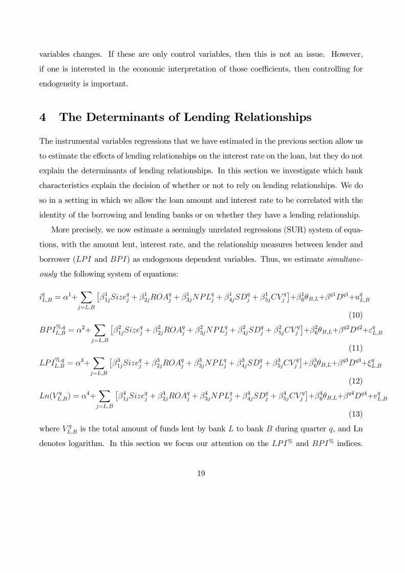
4 The Determinants of Lending Relationships
The instrumental variables regressions that we have estimated in the previous section allow us
to estimate the effects of lending relationships on the interest rate on the loan, but they do not
explain the determinants of lending relationships. In this section we investigate which bank
characteristics explain the decision of whether or not to rely on lending relationships. We do
so in a setting in which we allow the loan amount and interest rate to be correlated with the
identity of the borrowing and lending banks or on whether they have a lending relationship.
More precisely, we now estimate a seemingly unrelated regressions (SUR) system of equa-
tions, with the amount lent, interest rate, and the relationship measures between lender and
borrower (LPI and BPI) as endogenous dependent variables. Thus, we estimate simultane-
ously the following system of equations:
iqL,B = α1+Xj=L,B
£β11jSize
qj + β12jROA
qj + β13jNPLq
j + β14jSDqj + β15jCV
qj
¤+β16θB,L+β
q1Dq1+uqL,B
(10)
BPI%,qL,B = α2+Xj=L,B
£β21jSize
qj + β22jROA
qj + β23jNPLq
j + β24jSDqj + β25jCV
qj
¤+β26θB,L+β
q2Dq2+εqL,B
(11)
LPI%,qL,B = α3+Xj=L,B
£β31jSize
qj + β32jROA
qj + β33jNPLq
j + β34jSDqj + β35jCV
qj
¤+β36θB,L+β
q3Dq3+ξqL,B
(12)
Ln(V qL,B) = α4+
Xj=L,B
£β41jSize
qj + β42jROA
qj + β43jNPLq
j + β44jSDqj + β45jCV
qj
¤+β46θB,L+β
q4Dq4+vqL,B
(13)
where V qL,B is the total amount of funds lent by bank L to bank B during quarter q, and Ln
denotes logarithm. In this section we focus our attention on the LPI% and BPI% indices.
19

The results for the LPI# and BPI# are similar and reported in section 6. We estimate a
reduced form system, and therefore allow for contemporaneous correlation across the different
innovations (u, ε, ξ and v). As before, we include time dummies in all equations.
4.1 BPI and LPI equations
Table 6 shows the estimation results for BPI% and LPI% indices. The results for the BPI%
equation are shown in the second column. In this equation we try to determine which borrower
and lender characteristics explain the variation in BPI% indices. In other words, who are the
borrowers’ who have higher relationship indices, and who are the lenders with whom they
have higher indices.
The negative coefficient on the logarithm of total assets of borrowers means that small
borrowers rely more on lending relationships. The estimated coefficient on the total assets of
lender in the BPI% equation is positive and statistically significant, meaning that small bor-
rowers tend to have large banks as their preferred lenders. These results suggest a dichothomy
between large and small banks in the market, an issue that we explore further in section 5.1.
Interestingly, we find that borrowers with higher default risk are more likely to rely on
lending relationships: the estimated coefficient on NPL of borrowers is positive and significant.
In addition, borrowers with a large proportion of NPL pay higher interest rates on their loans
(the estimated coefficient on NPL in the interest rate equation is positive). From these two
results one may reasonably expect that banks which borrow funds from banks with whom
they have a lending relationship pay higher rates. This may seem inconsistent with the result
in Table 4 that loan rates tend to be lower for banks borrowing from lenders with whom they
have large relationship indices.
The key to understanding this apparent inconsistency is to note that we do not find that
unconditionally borrowers with a high default risk and large BPI indices pay lower interest
rates. In fact the reverse is true: large values for BPI indices tend to be associated with higher
interest rates (Table 3, and column (i) in Table 4). It is only when controlling for default risk
20
that the estimated coefficient on the BPI index is negative (Table 4 column (ii)), but even so
it is an order of magnitude smaller than the coefficient on the default risk variable. That is:
borrowers with a high proportion of NPL pay on average higher interest rates. However, the
interest rate premium is smaller if they borrow funds from a lender with whom they have a
high BPI.
Some calculations help to clarify this important point. Consider an increase in the pro-
portion of NPL from the 25th to the 75th percentile, while everything else remains the same.
Using the estimated coefficients in the third column of table 4 we see that the interest rate
on the loan increases by 2 basis points.14 However, if the increase in the proportion of NPL is
accompanied by an increase in the BPI index from the 25th to the 75th percentile, the increase
in interest rate is only 0.6 basis points. If instead we consider an increase in the proportion of
NPL from the 10th to the 90th percentile the increase in interest rate is 20 basis points when
the BPI index is unchanged, and 5 basis points when the BPI index also increases from the
10th to the 90th percentile.15
Several of the insurance variables are also significant. The estimated negative coefficient
on the surplus deposit of borrowers implies that they are more likely to borrow funds from
lenders with whom they have large relationship indices when they have a larger shortage of
funds. Borrowers with more volatile liquidity shocks tend to rely more on lending relationships
(the coefficient on CV qB is positive), and they tend to do so with lenders that have less volatile
liquidity shocks (the estimated coefficient on CV qL in the BPI% equation is negative and
statistically significant). This supports the idea that lending relationships are important for
insurance purposes. Finally, the correlation variable is also significant and it has a negative
coefficient, which is consistent with the mutual insurance hypothesis. Borrowers are more likely
to have lending relationships with lenders when their liquidity shocks are less correlated. In
14Due to our scaling of the dependent variable we need to multiply the increase by the standard deviation
of the interest rate.15The effect of NPL on the interest rate may be larger because default risk is likely to be correlated with
bank size, for which we are also controlling in Table 4.
21
such case the insurance benefits of the relationship are likely to be larger.
The third column of Table 6 reports the results for the LPI% equation. Similarly to the
borrowers, we find that small lenders are more likely to have higher relationships indices, and
that they tend to do so higher indices with large borrowers (the estimated coefficient on total
assets of lenders is negative and on the total assets of borrowers is positive). The estimated
coefficient on the credit risk of lenders is not statistical significant. This is consistent with the
results for the interest rate regression reported in Table 4. It is natural to expect that what
matters in a loan is the credit risk of the borrower, and not that of the lender.
In the LPI% equation, the estimated coefficient on the reserve imbalance of borrowers is
negative and statistically significant. This means that banks that borrow funds at times when
their reserve imbalance is larger tend to borrow funds from lenders which have high relationship
indices with them (recall that the reserve imbalance variable for borrowers is defined in such a
way that a lower value means a higher imbalance). Thus loans that take place when reserves
imbalances are larger tend to be associated with higher relationship indices. This result comes
from the time-series dimension of our panel.
In addition, lenders with more volatile liquidity shocks tend to have higher relationship
indices with borrowers that face less volatile liquidity shocks, although the estimated coefficient
for borrowers is not significantly different from zero. As in the BPI% equation, the estimated
coefficient on the correlation variable is negative, consistent with the mutual insurance motive
for establishing relationships.
As a whole, columns two and three of Table 6 show that it is mostly borrower characteristics
that explain variation in the BPI% and LPI% indices. Among the lender characteristics the
only two that seem to be important are the logarithm of total assets and liquidity risk. One
might have an a priori expectation that for non-secure loans such as interbank market loans,
borrowers’ characteristics are more important for explaining the terms of the loan than lenders’
characteristics. Table 6 suggests that this reasoning carries through when explaining lending
relationships.
22
4.2 Interest rate and loan volume equations
The fourth column of Table 6 shows the results for the interest rate equation. This equation
is similar to that estimated in specification (iii) of Table 4, except that now we do not include
the LPI and BPI indices as independent variables, but instead treat them as endogenous when
estimating the system of equations. The main noticeable difference relative to the results in
Table 4 is that the estimated coefficient for the borrower’s ROA is now non-significant. Given
that several papers on lending relationships rely on regressions of the price of the loan on
relationship measures and other control variables, it is re-assuring to find out that in our data
the results for this regression are robust to an approach that treats the relationship measures
as endogenous variables.
In the last column of Table 6 we report the results for loan volume (the fourth equation
in the SUR system). We find that larger banks borrow larger amounts. Interestingly, we
find that more profitable banks lend less (the estimated coefficients on ROAqL is negative).
In addition, we find that banks with a higher proportion of non-performing loans lend more
and borrow less (the estimated coefficients on NPLqL and NPLq
B are positive and negative,
respectively). The estimated coefficients for ROA and NPL are consistent with banks that
have better investment opportunities borrowing more and lending less. Finally, the estimated
coefficients on surplus deposit show that banks which have smaller imbalances tend to rely on
larger loans with any particular bank.
4.3 Correlation of residuals
At the bottom of Table 6 we show the estimated correlation matrix of residuals in the SUR
system of equations. This allows us to study the correlation between the different endoge-
nous variables. However, we should point out that since our SUR system is a reduced form
estimation, these correlations are not partial derivatives, i.e. when we look at the correlation
between the residuals in two different equations we are not holding the other endogenous
variables constant.
23
Larger residuals for the BPI equation are associated with lower interest rates, and larger
residuals for the LPI equation are associated with higher interest rates. Thus, borrowers
pay lower interest rates when they borrow funds from banks with whom they have a lending
relationship, and lenders receive a higher interest rate when they lend funds to banks with
whom they have a lending relationship. Although the signs of the correlations between the
LPI and BPI and interest rate are intuitive, the magnitude of the correlation is fairly small.
From Table 6 we see that the largest correlations are of amount lent with LPI and BPI, which
are equal to 0.44 and 0.31, respectively. This finding supports the idea that relationships have
the greatest effect on the provision of credit, and not on the price at which banks are able to
borrow or lend.
5 Further Evidence on the Determinants of Lending
Relationships
In this section we provide further evidence on the determinants of lending relationships, that
allows us to be more precise as to their exact nature.16
5.1 Small versus Large Banks
The estimation results in the previous sections show that bank size is an important determi-
nant of interbank market interest rates, and of lending relationships. In this section we explore
further the role of bank size in the market structure. In order to do so, and for each quarter
in our sample, we classify banks into large and small, based on the quarterly distribution of
bank assets. Large (small) banks are those whose assets are larger (smaller) than percentile
66 (33) of this distribution. We then compare several variables for small and large banks.
The first two rows of Table 7, Panel A report the average amount borrowed/lent per bank
16We would like to thank an anonymous referee for suggestions that have led us to investigate the questions
in this section.
24
and quarter over the whole sample period. The third row reports the net amount borrowed,
which is simply the difference between the first two. The second column shows the results for
all banks, i.e. not conditional on bank size, while columns three and four show the results for
small and large banks, respectively. On average, and per quarter, each bank in our sample
has lent/borrowed 596.5 million euros. There are significant differences between small and
large banks: large banks tend to be net borrowers, with an average net amount borrowed
roughly equal to 400 million euros, while small banks tend to be net lenders, with an average
net amount lent equal to 363 million euros.
Interestingly, this pattern of trade, in which large banks tend to be net buyers of liquidity
and small banks tend to be net sellers, is also a distinctive feature of the US Fed Funds market
(see for example Furfine, 1999, or Ho and Saunders, 1985).17 It can be rationalized by the
model of Ho and Saunders (1985). If large banks are better able to diversify their risk exposure
than small banks, then larger banks will be more rate sensitive than small banks, and the
slopes of the demand functions for interbank funds of large banks will be more price-elastic
than those of small banks. An important policy implication is that open market operations by
the central bank will be more effective when targeted at large rather than small institutions.
Table 7, Panel A also reports information on the number of loans and average loan amount.
Large (small) banks tend to transact mostly as borrowers (lenders), reflecting the fact that
they tend to be net borrowers (lenders) in the market. Unsurprisingly, average loan amount
for small banks is significantly lower than average loan amount for large banks.
The last three rows of Table 7, Panel A report the proportion of non-performing loans,
and relationship indices. Small banks tend to have a significantly higher proportion of non-
preforming loans than large banks. Furthermore, they tend to have significantly higher BPI
indices than large banks when borrowing funds. This suggests that small banks when bor-
rowing funds find it optimal to concentrate their borrowing. Interestingly, the same is not
17See also Stigum’s (1990) description of the Fed Funds market: “To cultivate correspondents that will sell
funds to them, large banks stand ready to buy whatever sums these banks offer, whether they need all these
funds or not."
25
true when lending funds, since there are no statistically significant differences in LPI indices
between small and large banks.
We have also investigate the likelihood that banks appear on both sides of the market, i.e.
as lenders and borrowers over a given time period. Panel B of Table 7 reports that 66.1%
(50.2%) of all banks have been on average active market participants on both sides of the
market at least once a month (week).
Panel B of Table 7 also reports summary statistics for bank assets and proportion of non-
performing loans as a function of how often banks appear on both sides of the market. It
shows that large banks are more likely to appear on both sides of the market, and in this way
act as intermediaries. In addition, banks that reverse their positions more frequently tend to
have a significantly lower proportion of non-performing loans. Naturally, banks with lower
credit risk are better-suited to act as intermediaries. Finally, we have investigated whether
the volatility of liquidity shocks differs depending on the frequency with which banks appear
on both sides of the market, but found no statistically significant differences.
Smaller banks are less likely to act as intermediaries, and are more likely to act as lenders.
But is it the case that when they need to borrow funds they do so from banks to whom they
usually lend funds? In order to investigate this we have estimated the probability that small
banks borrow funds from a bank to whom they usually lend funds, where the latter means a
bank in top fifty percent (one third) of the distribution of LPI indices for that small bank.
This probability is as high as 66.88% (54.58% for the one-third cutoff). The corresponding
probabilities for all banks, i.e. not conditional on bank size, are smaller and equal to 59.28%
(48.43%). Thus small banks, when reversing roles, tend to rely more on banks with whom
they usually interact on the other side of the market than the average bank in our sample.
5.2 International Linkages
Unfortunately our main dataset only includes information on loans in the domestic interbank
market. However, and in order to explore international linkages between domestic and foreign
26
banks, we have obtained data from a different dataset, namely from the Trans-European
Automated Real-time Gross settlement Express Transfer system (TARGET). This is the real-
time gross settlement system for the euro offered by the Eurosystem. It is mainly used for
the settlement of large-value euro interbank transfers. This dataset contains information on
the identity of both the sender and receiver of funds, and on the amount transferred. It has
some shortcomings. First, transfers of funds between a pair of banks may be due to a variety
of reasons, other than interbank loans. For example, if a large individual client of a foreign
bank decides to transfer funds to a domestic bank, this transfer of funds will show up in the
dataset, and cannot be distinguished from an interbank loan. Second, this dataset is only
available from 1999 onwards, or roughly the second half of the sample period.
We use this dataset to investigate how international linkages relate to the nature of lend-
ing relationships in the domestic interbank market. This is particularly interesting because
the Euro area seems to be characterized by a two-tier structure, in which only large banks
are usually able to access foreign interbank markets for liquidity, and in which small banks
tend to do their interbank business through large domestic banks (European Central Bank,
2000). With this in mind, we first construct a measure of access to international markets, by
calculating the total amount of funds that each domestic bank has received from plus sent
abroad during each quarter. We then scale this variable by bank size, as measured by total
bank assets.18
We think that this variable is a better measure of access to international markets, than
simply the difference between funds received from abroad and funds sent abroad scaled by
bank assets. This is because a domestic bank may find it easy to access international interbank
markets, but during a given time period it may neither be net borrower nor net lender in these
18We have calculated alternative measures of access to international markets equal to the total amount of
funds that each domestic bank has received from abroad during the quarter scaled by bank assets, and equal
to the total amount of funds that each domestic bank has sent abroad during the quarter scaled by bank
assets. The correlation coefficient between these two variables is 0.97, and the correlation coefficients between
them and the total amount of funds sent plus received from abroad scaled by bank assets are over 0.99.
27
markets. In this case the latter variable would be zero. We classify banks into low and high
access to international markets, according to this measure. Banks with high (low) access are
those in the top (bottom) one third of the distribution of this variable. Table 8 shows the
results for the mean of several variables for each of these two groups. The last column shows
the p-value for a t-test of equality of means.
The first row confirms the result that banks with better access to international markets
tend to be larger: the difference in total bank assets between the two groups is almost five-
fold. Interestingly, we find that banks with low access to international markets tend to have a
much higher proportion of non-performing loans. Furthermore, these banks, when borrowing
funds in the domestic interbank market, find it optimal to concentrate their loans: their BPI
indices are much higher than those with high access to international market. This result is
consistent with peer monitoring across borders being less efficient than at the domestic level,
as in the model of Freixas and Holthausen (2005). It suggests that in international unsecured
credit markets such as interbank markets, peer monitoring plays an important role in that
it allows liquidity to flow across borders. However, an alternative explanation is that large
banks are perceived by international markets as being too-big-too-fail, and for this reason
they can borrow internationally at low rates. In either case, our results suggest that domestic
regulators should direct their policies towards an improvement of the cross-border information
available, particularly so on small banks, so as to enhance cross-border market integration.
Finally, we find that banks with high access to international markets tend to have a lower
coefficient of variation of liquidity shocks, but the difference relative to banks with low access
to international markets is not statistically significant.
5.3 Time-series probabilities of repeated interactions
In order to better understand the time-series dimension of the relationship between borrowers
and lenders we estimate the probability of repeated interactions. More precisely, we estimate
the probability that a given lender (L) will lend funds to a given borrower (B) in the next k
28
days, that is from t+1 to t+ k, conditional on L having lent funds to B at t, and conditional
on both L and B lending and borrowing funds in the market in the next k days. Thus, we are
trying to answer the following question: given that B has borrowed from L at t, and given
that B needs funds again sometime within the next k trading days, how likely is it that it will
borrow from L again?
Before we turn to the estimation results let us first calculate what we should expect to
observe if the matching mechanism was completely random. The average number of loans on
a given day is 43.31, and the average daily number of active lenders in the market is 23.1.
This corresponds to an average of 1.87 loans per lender each day. Since the average daily
number of active borrowers is 17.95, if the matching was completely random the probability
of a lender lending to the same borrower at t+ 1, conditional on having done so at t and on
both lender and borrower being active in the market at t+ 1, is 10.2%.19 This probability is
roughly one fifth of the value that we have estimated in the data, and equal to 51% (Table
9, Panel A). This probability increases to 64% if we consider k equal to five, and if we take
a 30-day window the probability is as high as 87%. These probabilities are much larger than
those we would obtain with a random matching mechanism, which are 18% and 51% for a five
and a thirty-day window, respectively. The differences are statistically significant at the 1%
significance level. Thus, in the interbank market, lenders frequently use previous borrowers
and vice-versa, and much more frequently than one would obtain if the matching mechanism
was random.
With our previous analysis of bank size in mind, in Panel B of Table 9 we take this
analysis in that direction. In particular we estimate and find that the probability of repeated
interaction is higher if one of the banks is small (asset size below percentile 33) and the other
one is large (asset size above percentile 66). When both the borrower and the lender are
large the probability of repeated interaction is lower, and it is lowest when both lender and
19With probability 1/17.95 the bank lends to the same borrower in its first loan, plus with probability
(1−1/17.95) it does not lend to the same borrower in the first loan, but it does so with probability 0.87/17.95in the 0.87 remaining loan, so that the probability is 1/17.95 + (1− 1/17.95)× 0.87/17.95.
29
borrower are small. These estimated probabilities suggest that lending relationship are most
important when between small and large banks in the domestic market. In panel B of Table
9, below the estimated probabilities, we report whether these probabilities are statistically
different from one another. It is important to note that for k equal to one we do not find
that the probability of SS is significantly different than LL or LS because there are very few
observations for SS and k = 1.
6 Robustness checks
In Tables 10 through 11 we present several different robustness checks, in which we estimate
the SUR system using alternative measures of lending relationships. Table 10 reports the
estimation results for the previously constructed BPI# and LPI# indices. In interpreting
the results in this table one should recall that a higher index means that banks rely less on
lending relationships. That is the interpretation is symmetric to that of the BPI% and LPI%
indices. The results in Table 10 are similar to those in Table 6, except for the fact that in the
third column the NPL of lenders is positive and statistically significant. Thus lenders with
a higher NPL tend to rely more on lending relationships. This is the opposite of what one
might have a priori expected. However, this result is not robust to other relationship measures
(Tables 6 and 11).
We have constructed the LPI% as being equal to the total amount that bank L has lent to
bank B as a fraction of the total amount that bank L has lent in the interbank market during
the quarter. However, during the same quarter bank L may borrow funds from bank B. We
now investigate the robustness of the results to measures that take into account a two-sided
relationship factor. More precisely, the relationship measures are:
BPI2L,B,q =Xi∈q
¡FL−→Bi + FB−→L
i
¢/Xi∈q
¡F all−→Bi + FB−→all
i
¢(14)
LPI2L,B,q =Xi∈q
¡FL−→Bi + FB−→L
i
¢/Xi∈q
¡FL−→alli + F all−→L
i
¢(15)
30
Thus the borrower preference index is now defined as the total amount bank B borrowed from
plus lent to bank L divided by the total amount of funds that B has borrowed plus lent in the
market during quarter q. The estimation results for these alternative relationship measures
are reported in Table 11. Although there are some differences in magnitude and statistical
significance of some of the estimated coefficients, the results are similar to those we obtained
before.
Finally, we have constructed lender and borrower preference indices similar to LPI% and
BPI% but using number of loans instead of loan amounts. That is the lender preference index
was constructed as the number of times that L has lent funds to B during quarter q, as a
fraction of the total number of times that bank L has lent funds in the interbank market
during the same quarter. The results were similar and are not reported.
7 Conclusion and Policy Implications
Interbank markets play an important role in distributing liquidity across the financial system.
It is in this market that banks borrow and lend funds among themselves, allowing for the
transfer of liquidity from banks that have excess funds to those that are short. However, since
interbank market loans are unsecured, they also increase the exposure of lenders to borrowers.
In this paper we have studied lending relationships in a typical interbank market.
There are at least two sets of reasons why banks may benefit from lending relationships.
First, in the models of Ho and Saunders (1985), Bhattacharya and Gale (1987), and Freixas,
Parigi and Rochet (2000) banks borrow and lend funds in the interbank market to insure
against idiosyncratic liquidity shocks that arise from the behavior of retail depositors. Thus,
banks may form lending relationships for insurance purposes. Second, Rochet and Tirole
(1996) present a model of the interbank market in which asymmetric information and mon-
itoring play an important role. Thus, banks may rely on lending relationships to overcome
problems that arise from asymmetric information on credit worthiness.
We have provided evidence that supports both of these motives for the existence of lending
31
relationships. Importantly, we have done so by explicitly recognizing that these relationships
are endogenous, and addressing the issue by estimating instrumental variables regressions and
a system of seemingly unrelated regressions. We have found that smaller banks, with lower
return on assets, banks with a higher proportion of non-performing loans and banks that are
subject to more volatile liquidity shocks rely more on lending relationships, and that they tend
to form relationships with large banks, and banks that are subject to less volatile liquidity
shocks.
In order to be more precise as to the exact nature of lending relationships, we have inves-
tigated the role of bank size in the market structure. Interestingly, we have found that large
banks tend to be net buyers of liquidity and small banks tend to be net sellers. This pattern of
trade is also a distinctive feature of the US Fed Funds market (see for example Furfine, 1999,
or Ho and Saunders, 1985). It can be rationalized by the model of Ho and Saunders (1985).
If large banks are better able to diversify their risk exposure than small banks, then large
banks will be more rate sensitive than small banks, and the slopes of the demand functions
for interbank funds of large banks will be more price-elastic than those of small banks. One
important policy implication is that open market operations by the central bank will be more
effective when targeted at large rather than small institutions.
We have also investigated how access to international markets affects the nature of lending
relationships in the domestic market. We have found that large domestic banks tend to
have better access to international markets. Interestingly, we have found that banks with low
access to international markets tend to have a much higher proportion of non-performing loans.
Furthermore, these banks, when borrowing in the domestic interbank market, find it optimal
to concentrate their loans. This result is consistent with peer monitoring across borders being
less efficient than at the domestic level, as in the model of Freixas and Holthausen (2005).
It suggests that in international unsecured credit markets such as interbank markets, peer
monitoring plays an important role in that it allows liquidity to flow across borders. However,
an alternative explanation is that large banks are perceived by international markets as being
too-big-too-fail, and for this reason they can borrow internationally. In either case, our results
32

suggest that domestic regulators should direct their policies towards an improvement of the
cross-border information available, particularly so on small banks, so as to enhance cross-
border market integration.
33
8 References
Allen, Franklin and Douglas Gale, 2000, “Financial Contagion,” Journal of Political Econ-
omy, 108, pp. 1-33.
Allen, Linda, and Anthony Saunders, 1986, “The Large-small Bank Dichotomy in The Federal
Funds Market,” Journal of Banking and Finance, 10, pp. 219-230.
Berger Allen N. and Gregory F. Udell, 1992, “Some Evidence on the Empirical Significance
of Credit Rationing,” Journal of Political Economy, 100, pp. 1047-1077.
Berger Allen N. and Gregory F. Udell, 1995, “Relationship Lending and Lines of Credit in
Small Firm Finance,” Journal of Business, 68, pp. 351-381.
Berlin, Mitchell, and Loretta Mester, 1999, “Deposits and Relationship Lending,” Review of
Financial Studies, 12, pp. 579-607.
Bhattacharya, Sudipto and Douglas Gale, 1987, Preference Shocks, Liquidity, and Central
Bank Policy, in W. Barnett and K. Singelton (eds.), New Approaches to Monetary
Economics, Cambridge University Press.
Biais, Bruno, 1993, “Price Formation and Equilibrium Liquidity in Fragmented and Central-
ized Markets,” Journal of Finance, 48, pp. 157-185.
Broecker, Thorsten, 1990, “Credit-Worthiness Tests and Interbank Competition," Econo-
metrica, 58, pp. 429-452.
Campbell, John, 1987, “Money Announcements, the Demand for Bank Reserves, and the
Behavior of the Federal Funds Rate within the Statement Week,” Journal of Money,
Credit and Banking, 19, pp. 56-67.
Elsas, Ralf, Frank Heinemann, and Marcel Tyrell, 2004, “Multiple But Asymmetric Bank Fi-
nancing: The Case of Relationship Lending,” working paper, Goethe-Universitat Frank-
furt.
34
European Central Bank, 2000, “The Euro Area One Year After the Introduction of the
Euro: Key Characteristics and Changes in The Financial Structure,” Monthly Bulletin,
January, 35-49
Flannery, Mark J., 1996, “Financial Crisis, Payment System and DiscountWindow Lending,"
Journal of Money Credit and Banking, 28, pp. 804-824.
Freixas, Xavier, and Cornelia Holthausen, 2005,“Interbank Market Integration under Asym-
metric Information,” Review of Financial Studies, 18, 2, 458-490.
Freixas, Xavier, Bruno Parigi and Jean-Charles Rochet, 2000, “Systemic Risk, Interbank
Relations and Liquidity Provision by the Central Bank,” Journal of Money Credit and
Banking, 32, pp. 611-638.
Furfine, Craig, 1999, “The Microstructure of the Federal Funds Market,” Financial Markets,
Institutions, and Instruments, 8, 24-44.
Furfine, Craig, 2001, “Banks as Monitors of Other Banks: Evidence from the Overnight
Federal Funds Market,” Journal of Business, 74, 33-57.
Hamilton, James, 1996, “The Daily Market for Federal Funds,” Journal of Political Economy,
104, 26-56.
Hartmann, Philipp, Michele Manna and Andrés Manzanares, “The microstructure of the
euro money market,” October 2001, ECB Working Paper No. 80.
Ho, Thomas and Anthony Saunders, 1985, “A Micro-Model of the Federal Funds Market,”
Journal of Finance, 40, 977-990.
O’Hara, Maureen, 1995, Market Microstructure Theory. Blackwell, Cambridge.
Ongena, Steven and David C. Smith, 2000, “Bank relationships: a review.” in Zenios, S.
A. and P. Harker (eds.), Performance of Financial Institutions, Cambridge University
Press, pp. 221-258.
35
Ongena, Steven and David C. Smith, 2001, “The duration of bank relationships,” Journal of
Financial Economics, 61, pp. 449-475.
Petersen, Mitchell, and Raghuram Rajan, 1995, “The Effect of Credit Market Competition
on Lending Relationships,” Quarterly Journal of Economics, 110, 407-443.
Petersen, Mitchell and Raghuram Rajan, 1994, “The Benefits of Lending Relationships:
Evidence from Small Business Data,” Journal of Finance, 49, 3-37.
Rochet, Jean-Charles and Jean Tirole, 1996, “Interbank Lending and Systemic Risk,” Journal
of Money Credit and Banking, 28, 733-762.
Slovin, Myron B., Marie E. Sushka, and John A. Poloncheck, 1993, “The Value of Bank
Durability: Borrowers versus Bank Stakeholders,” Journal of Finance, 48, pp. 298-302.
Spindt, Paul A., and Ronald Hoffmeister, 1988, “The Micromechanics of the Federal Funds
Market: Implications for Day of the Week Effects in Funds Rate Variability,” Journal
of Financial and Quantitive Analysis, 23, 401-416.
Stigum, Marcia, 1990, The Money Market, Dow-Jones Irwin.
Upper, Christian, 2004, “Survey of The Literature on Interbank Lending,” manuscript,
Deutsche Bundesbank.
Wolinsky, Asher, 1990, “Information Revelation in a Market with Pairwise Meetings,” Econo-
metrica, 58, 1-25.
36
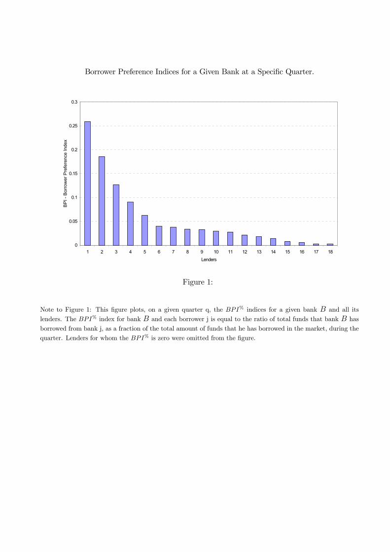
Borrower Preference Indices for a Given Bank at a Specific Quarter.
0
0.05
0.1
0.15
0.2
0.25
0.3
1 2 3 4 5 6 7 8 9 10 11 12 13 14 15 16 17 18Lenders
BP
I - B
orro
wer
Pre
fere
nce
Inde
x
Figure 1:
Note to Figure 1: This figure plots, on a given quarter q, the BPI% indices for a given bank B and all its
lenders. The BPI% index for bank B and each borrower j is equal to the ratio of total funds that bank B has
borrowed from bank j, as a fraction of the total amount of funds that he has borrowed in the market, during the
quarter. Lenders for whom the BPI% is zero were omitted from the figure.
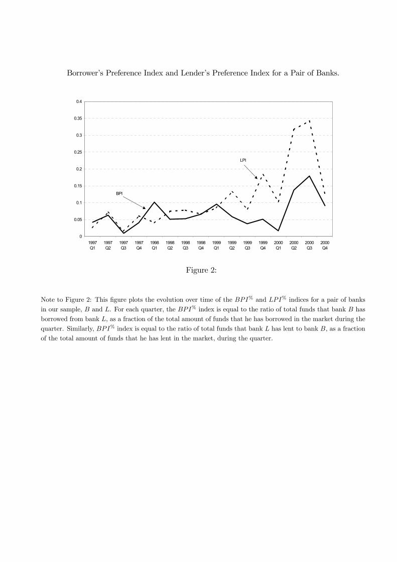
Borrower’s Preference Index and Lender’s Preference Index for a Pair of Banks.
0
0.05
0.1
0.15
0.2
0.25
0.3
0.35
0.4
1997Q1
1997Q2
1997Q3
1997Q4
1998Q1
1998Q2
1998Q3
1998Q4
1999Q1
1999Q2
1999Q3
1999Q4
2000Q1
2000Q2
2000Q3
2000Q4
BPI
LPI
Figure 2:
Note to Figure 2: This figure plots the evolution over time of the BPI% and LPI% indices for a pair of banks
in our sample, B and L. For each quarter, the BPI% index is equal to the ratio of total funds that bank B has
borrowed from bank L, as a fraction of the total amount of funds that he has borrowed in the market during the
quarter. Similarly, BPI% index is equal to the ratio of total funds that bank L has lent to bank B, as a fraction
of the total amount of funds that he has lent in the market, during the quarter.
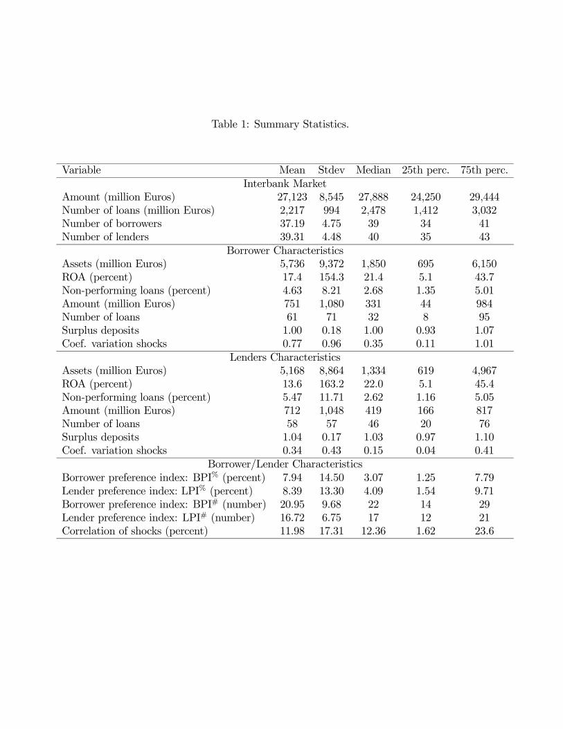
Table 1: Summary Statistics.
Variable Mean Stdev Median 25th perc. 75th perc.Interbank Market
Amount (million Euros) 27,123 8,545 27,888 24,250 29,444Number of loans (million Euros) 2,217 994 2,478 1,412 3,032Number of borrowers 37.19 4.75 39 34 41Number of lenders 39.31 4.48 40 35 43
Borrower CharacteristicsAssets (million Euros) 5,736 9,372 1,850 695 6,150ROA (percent) 17.4 154.3 21.4 5.1 43.7Non-performing loans (percent) 4.63 8.21 2.68 1.35 5.01Amount (million Euros) 751 1,080 331 44 984Number of loans 61 71 32 8 95Surplus deposits 1.00 0.18 1.00 0.93 1.07Coef. variation shocks 0.77 0.96 0.35 0.11 1.01
Lenders CharacteristicsAssets (million Euros) 5,168 8,864 1,334 619 4,967ROA (percent) 13.6 163.2 22.0 5.1 45.4Non-performing loans (percent) 5.47 11.71 2.62 1.16 5.05Amount (million Euros) 712 1,048 419 166 817Number of loans 58 57 46 20 76Surplus deposits 1.04 0.17 1.03 0.97 1.10Coef. variation shocks 0.34 0.43 0.15 0.04 0.41
Borrower/Lender CharacteristicsBorrower preference index: BPI% (percent) 7.94 14.50 3.07 1.25 7.79Lender preference index: LPI% (percent) 8.39 13.30 4.09 1.54 9.71Borrower preference index: BPI# (number) 20.95 9.68 22 14 29Lender preference index: LPI# (number) 16.72 6.75 17 12 21Correlation of shocks (percent) 11.98 17.31 12.36 1.62 23.6
Note to Table 1: This table reports summary statistics for overnight loans and main characteristics of borrowers
and lenders in the Portuguese Interbank market. The sample period is January 1997 to August 2001. Amount
is the total volume of overnight loans during a quarter (corrected for double counting) in millions of Euros and
number of loans the total number of overnight loans during a quarter. Number of borrowers (lenders) is the
number of different borrowing (lending) banks during the quarter. Assets is the value of total assets of the bank
at the beginning of each quarter in millions of Euros; ROA is the ratio between the annualized quarterly returns
and the bank’s total assets expressed in percentage terms; Non-performing loans is the percentage of past due
loans (loans that are overdue for more than 90 days) on the total value of outstanding loans granted by the bank.
Amount is the total amount of overnight loans during the quarter, in millions of Euros. Number of loans is the
number of overnight loans for lenders (borrowers) during a quarter. Surplus deposits is the quarterly average
of the ratio between the current level of deposits in the reserve account (average since the start of the current
reserve requirement period until day i) and the reserve requirements of the period. Correlation of shocks is the
correlation between the daily changes in the daily central bank deposits (not including the interbank market
operations) of the lender and the borrower. Coefficient of variation of shocks of borrower (lender) is the standard
deviation of the daily changes in the bank’s reserve deposits not due to interbank market loans scaled by bank’s
quarterly reserves. The Borrower (Lender) preference index BPI%(LPI
%) is equal to the ratio of total funds that
the bank has borrowed (lent) from a specific lender (borrower) as a fraction of the total amount of funds that
he has borrowed (lent) in the market during a quarter. The Borrower (Lender) preference index BPI#(LPI
#) is
defined as the total number of banks from (to) which the bank has borrowed (lent) funds during the quarter.
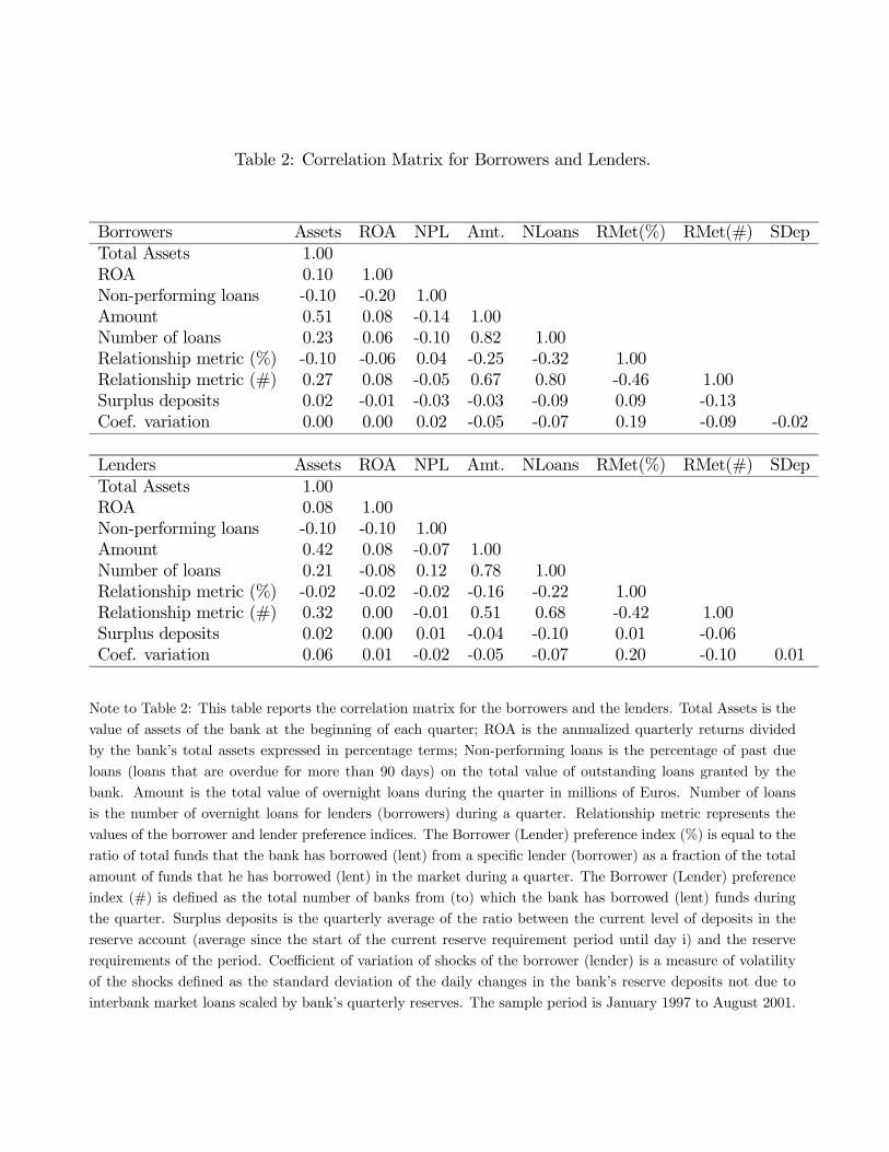
Table 2: Correlation Matrix for Borrowers and Lenders.
Borrowers Assets ROA NPL Amt. NLoans RMet(%) RMet(#) SDepTotal Assets 1.00ROA 0.10 1.00Non-performing loans -0.10 -0.20 1.00Amount 0.51 0.08 -0.14 1.00Number of loans 0.23 0.06 -0.10 0.82 1.00Relationship metric (%) -0.10 -0.06 0.04 -0.25 -0.32 1.00Relationship metric (#) 0.27 0.08 -0.05 0.67 0.80 -0.46 1.00Surplus deposits 0.02 -0.01 -0.03 -0.03 -0.09 0.09 -0.13Coef. variation 0.00 0.00 0.02 -0.05 -0.07 0.19 -0.09 -0.02
Lenders Assets ROA NPL Amt. NLoans RMet(%) RMet(#) SDepTotal Assets 1.00ROA 0.08 1.00Non-performing loans -0.10 -0.10 1.00Amount 0.42 0.08 -0.07 1.00Number of loans 0.21 -0.08 0.12 0.78 1.00Relationship metric (%) -0.02 -0.02 -0.02 -0.16 -0.22 1.00Relationship metric (#) 0.32 0.00 -0.01 0.51 0.68 -0.42 1.00Surplus deposits 0.02 0.00 0.01 -0.04 -0.10 0.01 -0.06Coef. variation 0.06 0.01 -0.02 -0.05 -0.07 0.20 -0.10 0.01
Note to Table 2: This table reports the correlation matrix for the borrowers and the lenders. Total Assets is the
value of assets of the bank at the beginning of each quarter; ROA is the annualized quarterly returns divided
by the bank’s total assets expressed in percentage terms; Non-performing loans is the percentage of past due
loans (loans that are overdue for more than 90 days) on the total value of outstanding loans granted by the
bank. Amount is the total value of overnight loans during the quarter in millions of Euros. Number of loans
is the number of overnight loans for lenders (borrowers) during a quarter. Relationship metric represents the
values of the borrower and lender preference indices. The Borrower (Lender) preference index (%) is equal to the
ratio of total funds that the bank has borrowed (lent) from a specific lender (borrower) as a fraction of the total
amount of funds that he has borrowed (lent) in the market during a quarter. The Borrower (Lender) preference
index (#) is defined as the total number of banks from (to) which the bank has borrowed (lent) funds during
the quarter. Surplus deposits is the quarterly average of the ratio between the current level of deposits in the
reserve account (average since the start of the current reserve requirement period until day i) and the reserve
requirements of the period. Coefficient of variation of shocks of the borrower (lender) is a measure of volatility
of the shocks defined as the standard deviation of the daily changes in the bank’s reserve deposits not due to
interbank market loans scaled by bank’s quarterly reserves. The sample period is January 1997 to August 2001.
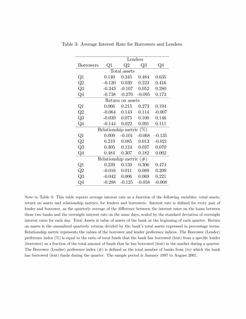
Table 3: Average Interest Rate for Borrowers and Lenders.
LendersBorrowers Q1 Q2 Q3 Q4
Total assetsQ1 0.140 0.345 0.484 0.635Q2 -0.120 0.039 0.223 0.416Q3 -0.343 -0.107 0.052 0.280Q4 -0.738 -0.270 -0.095 0.173
Return on assetsQ1 0.066 0.215 0.273 0.194Q2 -0.064 0.143 0.114 -0.007Q3 -0.039 0.075 0.100 0.146Q4 -0.144 0.022 0.091 0.111
Relationship metric (%)Q1 0.009 -0.101 -0.068 -0.135Q2 0.219 0.085 0.013 -0.021Q3 0.305 0.124 0.037 0.070Q4 0.484 0.307 0.182 0.002
Relationship metric (#)Q1 0.239 0.150 0.306 0.474Q2 -0.016 0.011 0.089 0.209Q3 -0.042 0.006 0.069 0.221Q4 -0.288 -0.125 -0.058 -0.008
Note to Table 3: This table reports average interest rate as a function of the following variables: total assets,
return on assets and relationship metrics, for lenders and borrowers. Interest rate is defined for every pair of
lender and borrower, as the quarterly average of the difference between the interest rates on the loans between
those two banks and the overnight interest rate on the same days, scaled by the standard deviation of overnight
interest rates for each day. Total Assets is value of assets of the bank at the beginning of each quarter. Return
on assets is the annualized quarterly returns divided by the bank’s total assets expressed in percentage terms.
Relationship metric represents the values of the borrower and lender preference indices. The Borrower (Lender)
preference index (%) is equal to the ratio of total funds that the bank has borrowed (lent) from a specific lender
(borrower) as a fraction of the total amount of funds that he has borrowed (lent) in the market during a quarter.
The Borrower (Lender) preference index (#) is defined as the total number of banks from (to) which the bank
has borrowed (lent) funds during the quarter. The sample period is January 1997 to August 2001.
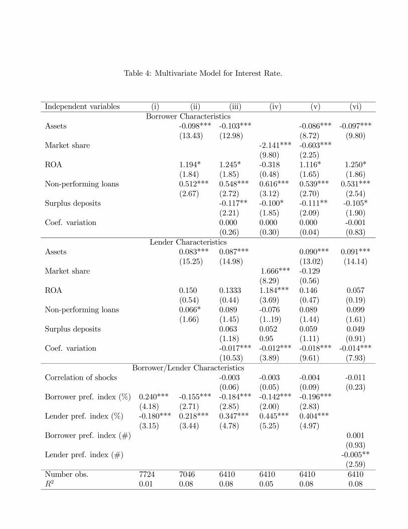
Table 4: Multivariate Model for Interest Rate.
Independent variables (i) (ii) (iii) (iv) (v) (vi)Borrower Characteristics
Assets -0.098*** -0.103*** -0.086*** -0.097***(13.43) (12.98) (8.72) (9.80)
Market share -2.141*** -0.603***(9.80) (2.25)
ROA 1.194* 1.245* -0.318 1.116* 1.250*(1.84) (1.85) (0.48) (1.65) (1.86)
Non-performing loans 0.512*** 0.548*** 0.616*** 0.539*** 0.531***(2.67) (2.72) (3.12) (2.70) (2.54)
Surplus deposits -0.117** -0.100* -0.111** -0.105*(2.21) (1.85) (2.09) (1.90)
Coef. variation 0.000 0.000 0.000 -0.001(0.26) (0.30) (0.04) (0.83)
Lender CharacteristicsAssets 0.083*** 0.087*** 0.090*** 0.091***
(15.25) (14.98) (13.02) (14.14)Market share 1.666*** -0.129
(8.29) (0.56)ROA 0.150 0.1333 1.184*** 0.146 0.057
(0.54) (0.44) (3.69) (0.47) (0.19)Non-performing loans 0.066* 0.089 -0.076 0.089 0.099
(1.66) (1.45) (1..19) (1.44) (1.61)Surplus deposits 0.063 0.052 0.059 0.049
(1.18) 0.95 (1.11) (0.91)Coef. variation -0.017*** -0.012*** -0.018*** -0.014***
(10.53) (3.89) (9.61) (7.93)Borrower/Lender Characteristics
Correlation of shocks -0.003 -0.003 -0.004 -0.011(0.06) (0.05) (0.09) (0.23)
Borrower pref. index (%) 0.240*** -0.155*** -0.184*** -0.142*** -0.196***(4.18) (2.71) (2.85) (2.00) (2.83)
Lender pref. index (%) -0.180*** 0.218*** 0.347*** 0.445*** 0.404***(3.15) (3.44) (4.78) (5.25) (4.97)
Borrower pref. index (#) 0.001(0.93)
Lender pref. index (#) -0.005**(2.59)
Number obs. 7724 7046 6410 6410 6410 6410R2 0.01 0.08 0.08 0.05 0.08 0.08
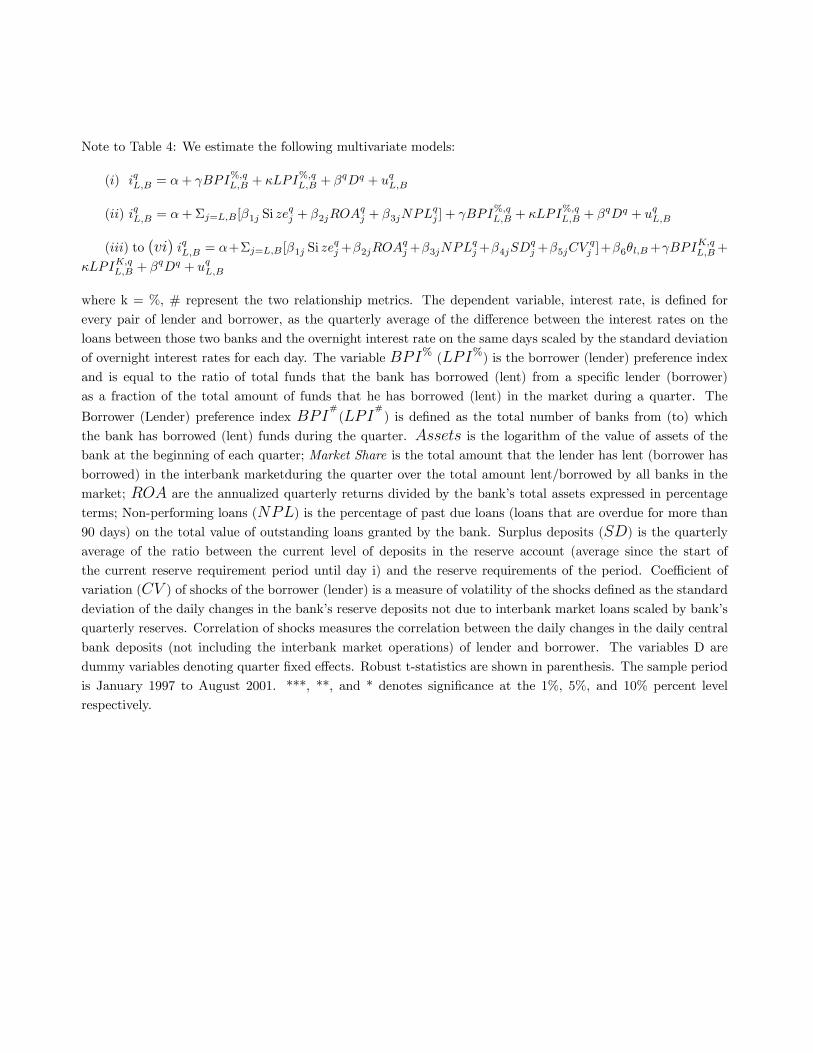
Note to Table 4: We estimate the following multivariate models:
(i) iqL,B = α+ γBPI%,qL,B + κLPI%,qL,B + βqDq + uqL,B
(ii) iqL,B = α+Σj=L,B[β1j Si zeqj + β2jROA
qj + β3jNPLqj ] + γBPI%,qL,B + κLPI%,qL,B + βqDq + uqL,B
(iii) to (vi) iqL,B = α+Σj=L,B [β1j Si zeqj+β2jROA
qj+β3jNPLqj+β4jSD
qj +β5jCV
qj ]+β6θl,B+γBPIK,q
L,B+
κLPIK,qL,B + βqDq + uqL,B
where k = %, # represent the two relationship metrics. The dependent variable, interest rate, is defined for
every pair of lender and borrower, as the quarterly average of the difference between the interest rates on the
loans between those two banks and the overnight interest rate on the same days scaled by the standard deviation
of overnight interest rates for each day. The variable BPI% (LPI%) is the borrower (lender) preference indexand is equal to the ratio of total funds that the bank has borrowed (lent) from a specific lender (borrower)
as a fraction of the total amount of funds that he has borrowed (lent) in the market during a quarter. The
Borrower (Lender) preference index BPI#
(LPI#
) is defined as the total number of banks from (to) which
the bank has borrowed (lent) funds during the quarter. Assets is the logarithm of the value of assets of the
bank at the beginning of each quarter; Market Share is the total amount that the lender has lent (borrower has
borrowed) in the interbank marketduring the quarter over the total amount lent/borrowed by all banks in the
market; ROA are the annualized quarterly returns divided by the bank’s total assets expressed in percentage
terms; Non-performing loans (NPL) is the percentage of past due loans (loans that are overdue for more than90 days) on the total value of outstanding loans granted by the bank. Surplus deposits (SD) is the quarterlyaverage of the ratio between the current level of deposits in the reserve account (average since the start of
the current reserve requirement period until day i) and the reserve requirements of the period. Coefficient of
variation (CV ) of shocks of the borrower (lender) is a measure of volatility of the shocks defined as the standarddeviation of the daily changes in the bank’s reserve deposits not due to interbank market loans scaled by bank’s
quarterly reserves. Correlation of shocks measures the correlation between the daily changes in the daily central
bank deposits (not including the interbank market operations) of lender and borrower. The variables D are
dummy variables denoting quarter fixed effects. Robust t-statistics are shown in parenthesis. The sample period
is January 1997 to August 2001. ***, **, and * denotes significance at the 1%, 5%, and 10% percent level
respectively.
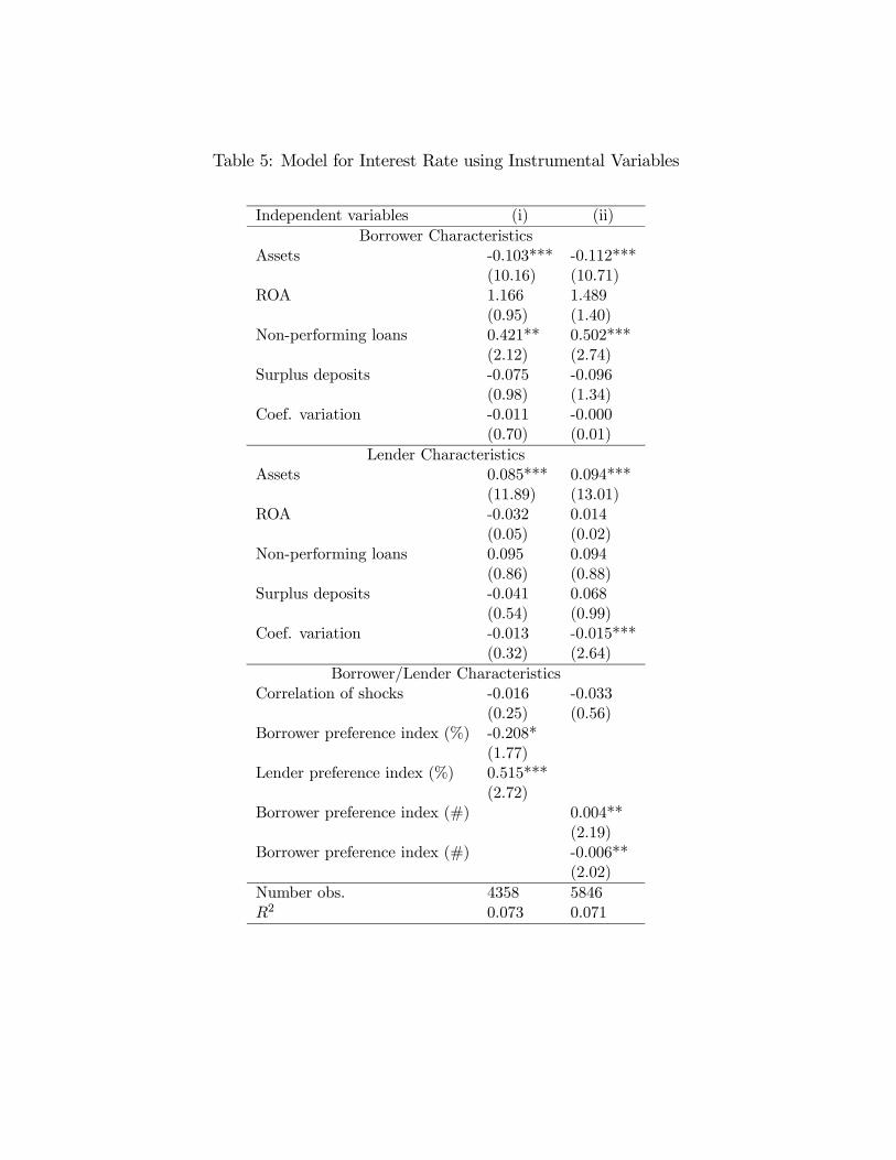
Table 5: Model for Interest Rate using Instrumental Variables
Independent variables (i) (ii)Borrower Characteristics
Assets -0.103*** -0.112***(10.16) (10.71)
ROA 1.166 1.489(0.95) (1.40)
Non-performing loans 0.421** 0.502***(2.12) (2.74)
Surplus deposits -0.075 -0.096(0.98) (1.34)
Coef. variation -0.011 -0.000(0.70) (0.01)
Lender CharacteristicsAssets 0.085*** 0.094***
(11.89) (13.01)ROA -0.032 0.014
(0.05) (0.02)Non-performing loans 0.095 0.094
(0.86) (0.88)Surplus deposits -0.041 0.068
(0.54) (0.99)Coef. variation -0.013 -0.015***
(0.32) (2.64)Borrower/Lender Characteristics
Correlation of shocks -0.016 -0.033(0.25) (0.56)
Borrower preference index (%) -0.208*(1.77)
Lender preference index (%) 0.515***(2.72)
Borrower preference index (#) 0.004**(2.19)
Borrower preference index (#) -0.006**(2.02)
Number obs. 4358 5846R2 0.073 0.071
Note to Table 5: We estimate the following model:
iqL,B = α+Σj=L,B [β1j Si zeqj +β2jROA
qj +β3jNPLqj +β4jSD
qj +β5jCV
qj ]+β6θl,B+γBPIk,qL,B+κLPIk,qL,B+
βqDq + uqL,B
using the variables BPIk,t−1L,B and LPIk,t−1L,B as instruments for BPIk,tL,B and LPIk,tL,B , respectively, and where
k = %,# are the two relationship metrics. The dependent variable, interest rate, is defined for every pair of lenderand borrower, as the quarterly average of the difference between the interest rates on the loans between thosetwo banks and the overnight interest rate on the same days scaled by the standard deviation of overnight interestrates for each day. The variable BPI% (LPI%) is the borrower (lender) preference index and is equal to theratio of total funds that the bank has borrowed (lent) from a specific lender (borrower) as a fraction of the totalamount of funds that he has borrowed (lent) in the market during a quarter. The Borrower (Lender) preferenceindex BPI
#(LPI
#) is defined as the total number of banks from (to) which the bank has borrowed (lent) funds
during the quarter. Assets is the logarithm of the value of assets of the bank at the beginning of each quarter;ROA are the annualized quarterly returns divided by the bank’s total assets expressed in percentage terms;Non-performing loans (NPL) is the percentage of past due loans (loans that are overdue for more than 90 days)on the total value of outstanding loans granted by the bank. Surplus deposits (SD) is the quarterly averageof the ratio between the current level of deposits in the reserve account (average since the start of the currentreserve requirement period until day i) and the reserve requirements of the period. Coefficient of variation (CV )of shocks of the borrower (lender) is a measure of volatility of the shocks defined as the standard deviation ofthe daily changes in the bank’s reserve deposits not due to interbank market loans scaled by bank’s quarterlyreserves. Correlation of shocks measures the correlation between the daily changes in the daily central bankdeposits (not including the interbank market operations) of lender and borrower. The variables D are dummyvariables denoting quarter fixed effects. Robust t-statistics are shown in parenthesis and are corrected for first-stage estimation error. The sample period is January 1997 to August 2001. ***, **, and * denotes significanceat the 1%, 5%, and 10% percent level respectively.
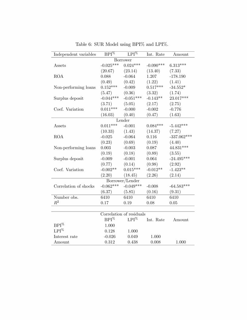
Table 6: SUR Model using BPI% and LPI%.
Independent variables BPI% LPI% Int. Rate AmountBorrower
Assets -0.025*** 0.024*** -0.090*** 6.313***(20.67) (23.14) (13.40) (7.33)
ROA 0.088 -0.064 1.207 -178.190(0.49) (0.42) (1.22) (1.41)
Non-performing loans 0.152*** -0.009 0.517*** -34.552*(5.47) (0.36) (3.32) (1.74)
Surplus deposit -0.044*** -0.051*** -0.143** 23.017***(3.71) (5.05) (2.17) (2.75)
Coef. Variation 0.011*** -0.000 -0.002 -0.776(16.03) (0.40) (0.47) (1.63)
LenderAssets 0.011*** -0.001 0.084*** -5.442***
(10.33) (1.43) (14.37) (7.27)ROA -0.025 -0.064 0.116 -337.062***
(0.23) (0.69) (0.19) (4.40)Non-performing loans 0.003 -0.003 0.087 44.831***
(0.19) (0.18) (0.89) (3.55)Surplus deposit -0.009 -0.001 0.064 -24.495***
(0.77) (0.14) (0.98) (2.92)Coef. Variation -0.002** 0.015*** -0.012** -1.423**
(2.20) (18.45) (2.26) (2.14)Borrower/Lender
Correlation of shocks -0.062*** -0.049*** -0.008 -64.583***(6.37) (5.85) (0.16) (9.31)
Number obs. 6410 6410 6410 6410R2 0.17 0.19 0.08 0.05
Correlation of residualsBPI% LPI% Int. Rate Amount
BPI% 1.000LPI% 0.128 1.000Interest rate -0.026 0.049 1.000Amount 0.312 0.438 0.008 1.000
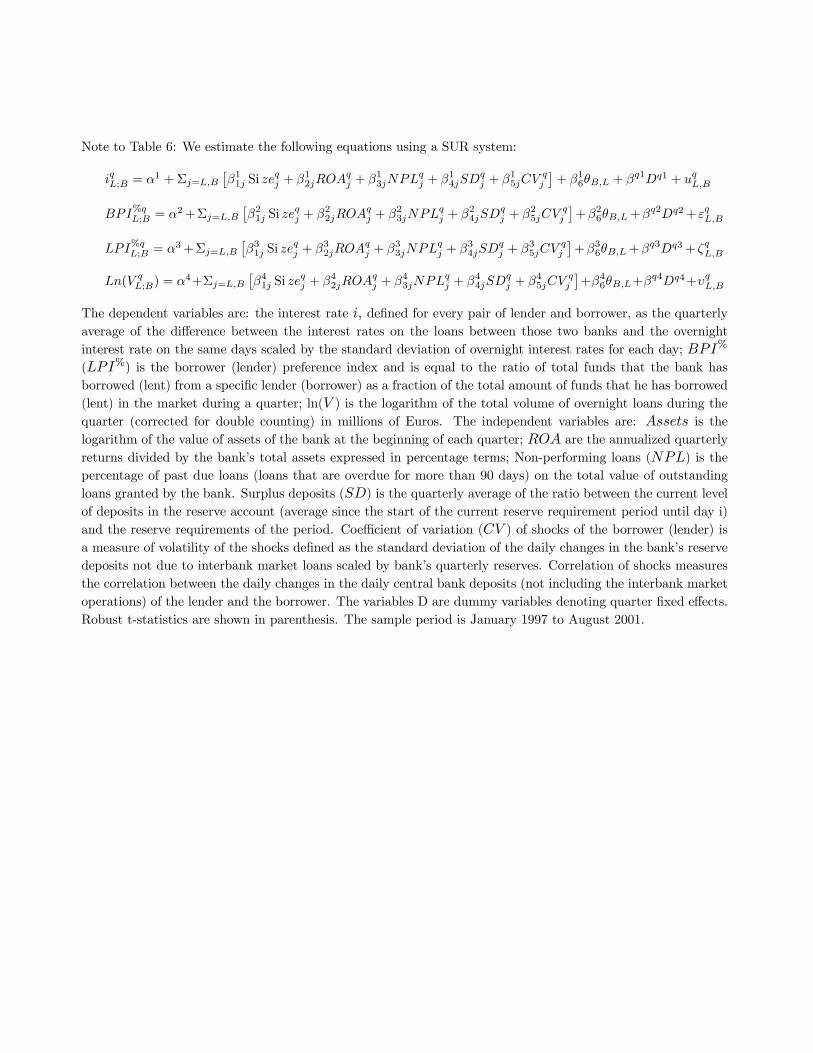
Note to Table 6: We estimate the following equations using a SUR system:
iqL;B = α1 +Σj=L,B£β11j Si ze
qj + β12jROA
qj + β13jNPLqj + β14jSD
qj + β15jCV
qj
¤+ β16θB,L + βq1Dq1 + uqL,B
BPI%qL;B = α2+Σj=L,B£β21j Si ze
qj + β22jROA
qj + β23jNPLqj + β24jSD
qj + β25jCV
qj
¤+β26θB,L+βq2Dq2+εqL,B
LPI%qL;B = α3+Σj=L,B£β31j Si ze
qj + β32jROA
qj + β33jNPLqj + β34jSD
qj + β35jCV
qj
¤+β36θB,L+βq3Dq3+ ζqL,B
Ln(V qL;B) = α4+Σj=L,B
£β41j Si ze
qj + β42jROA
qj + β43jNPLqj + β44jSD
qj + β45jCV
qj
¤+β46θB,L+β
q4Dq4+υqL,B
The dependent variables are: the interest rate i, defined for every pair of lender and borrower, as the quarterlyaverage of the difference between the interest rates on the loans between those two banks and the overnightinterest rate on the same days scaled by the standard deviation of overnight interest rates for each day; BPI%
(LPI%) is the borrower (lender) preference index and is equal to the ratio of total funds that the bank hasborrowed (lent) from a specific lender (borrower) as a fraction of the total amount of funds that he has borrowed(lent) in the market during a quarter; ln(V ) is the logarithm of the total volume of overnight loans during thequarter (corrected for double counting) in millions of Euros. The independent variables are: Assets is thelogarithm of the value of assets of the bank at the beginning of each quarter; ROA are the annualized quarterlyreturns divided by the bank’s total assets expressed in percentage terms; Non-performing loans (NPL) is thepercentage of past due loans (loans that are overdue for more than 90 days) on the total value of outstandingloans granted by the bank. Surplus deposits (SD) is the quarterly average of the ratio between the current levelof deposits in the reserve account (average since the start of the current reserve requirement period until day i)and the reserve requirements of the period. Coefficient of variation (CV ) of shocks of the borrower (lender) isa measure of volatility of the shocks defined as the standard deviation of the daily changes in the bank’s reservedeposits not due to interbank market loans scaled by bank’s quarterly reserves. Correlation of shocks measuresthe correlation between the daily changes in the daily central bank deposits (not including the interbank marketoperations) of the lender and the borrower. The variables D are dummy variables denoting quarter fixed effects.Robust t-statistics are shown in parenthesis. The sample period is January 1997 to August 2001.
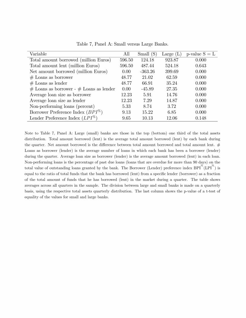
Table 7, Panel A: Small versus Large Banks.
Variable All Small (S) Large (L) p-value S = LTotal amount borrowed (million Euros) 596.50 124.18 923.87 0.000Total amount lent (million Euros) 596.50 487.44 524.18 0.643Net amount borrowed (million Euros) 0.00 -363.26 399.69 0.000# Loans as borrower 48.77 21.02 62.59 0.000# Loans as lender 48.77 66.91 35.24 0.000# Loans as borrower - # Loans as lender 0.00 -45.89 27.35 0.000Average loan size as borrower 12.23 5.91 14.76 0.000Average loan size as lender 12.23 7.29 14.87 0.000Non-performing loans (percent) 5.33 8.74 3.72 0.000Borrower Preference Index (BPI%) 9.13 15.22 6.85 0.000Lender Preference Index (LPI%) 9.65 10.13 12.06 0.148
Note to Table 7, Panel A: Large (small) banks are those in the top (bottom) one third of the total assets
distribution. Total amount borrowed (lent) is the average total amount borrowed (lent) by each bank during
the quarter. Net amount borrowed is the difference between total amount borrowed and total amount lent. #
Loans as borrower (lender) is the average number of loans in which each bank has been a borrower (lender)
during the quarter. Average loan size as borrower (lender) is the average amount borrowed (lent) in each loan.
Non-performing loans is the percentage of past due loans (loans that are overdue for more than 90 days) on the
total value of outstanding loans granted by the bank. The Borrower (Lender) preference index BPI%(LPI
%) is
equal to the ratio of total funds that the bank has borrowed (lent) from a specific lender (borrower) as a fraction
of the total amount of funds that he has borrowed (lent) in the market during a quarter. The table shows
averages across all quarters in the sample. The division between large and small banks is made on a quarterly
basis, using the respective total assets quarterly distribution. The last column shows the p-value of a t-test of
equality of the values for small and large banks.

Table 7, Panel B: Frequency of Borrowing and Lending Positions.
Frequency on both Proportion Bank Assets Non-Performingsides of the market of banks (million of euros) LoansAt least once a month 66.1% 6,058 5.53%At least once every two weeks 61.3% 6,395 4.72%At least once a week 50.2% 7,271 4.42%At least twice a week 38.7% 8,420 4.20%
Note to Table 7, Panel B: This table shows the proportion of banks that appear on both sides of the market, i.e.
as lenders and borrowers, over a given time period. The last two columns report the average bank assets and
the proportion of non-performing loans for banks that on average appear on both sides of the market over the
corresponding time period.
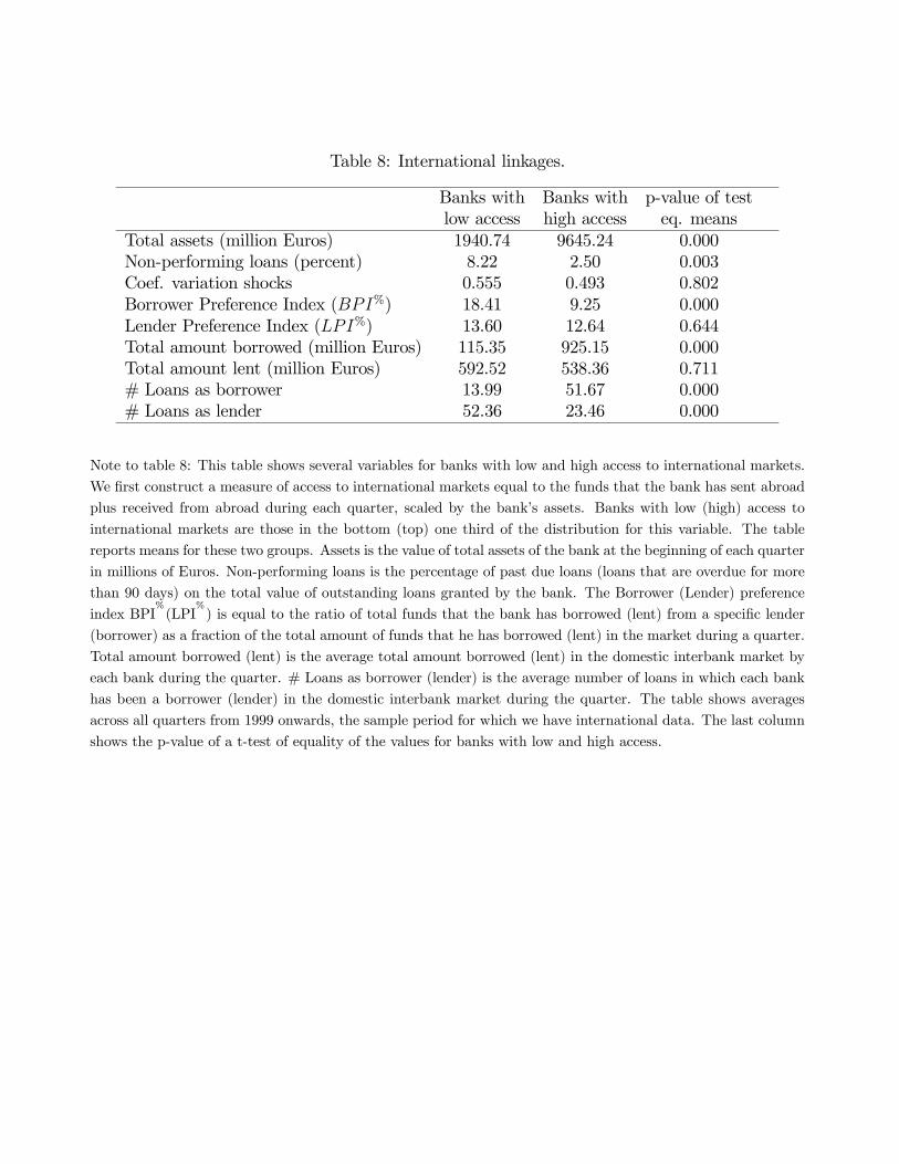
Table 8: International linkages.
Banks with Banks with p-value of testlow access high access eq. means
Total assets (million Euros) 1940.74 9645.24 0.000Non-performing loans (percent) 8.22 2.50 0.003Coef. variation shocks 0.555 0.493 0.802Borrower Preference Index (BPI%) 18.41 9.25 0.000Lender Preference Index (LPI%) 13.60 12.64 0.644Total amount borrowed (million Euros) 115.35 925.15 0.000Total amount lent (million Euros) 592.52 538.36 0.711# Loans as borrower 13.99 51.67 0.000# Loans as lender 52.36 23.46 0.000
Note to table 8: This table shows several variables for banks with low and high access to international markets.
We first construct a measure of access to international markets equal to the funds that the bank has sent abroad
plus received from abroad during each quarter, scaled by the bank’s assets. Banks with low (high) access to
international markets are those in the bottom (top) one third of the distribution for this variable. The table
reports means for these two groups. Assets is the value of total assets of the bank at the beginning of each quarter
in millions of Euros. Non-performing loans is the percentage of past due loans (loans that are overdue for more
than 90 days) on the total value of outstanding loans granted by the bank. The Borrower (Lender) preference
index BPI%(LPI
%) is equal to the ratio of total funds that the bank has borrowed (lent) from a specific lender
(borrower) as a fraction of the total amount of funds that he has borrowed (lent) in the market during a quarter.
Total amount borrowed (lent) is the average total amount borrowed (lent) in the domestic interbank market by
each bank during the quarter. # Loans as borrower (lender) is the average number of loans in which each bank
has been a borrower (lender) in the domestic interbank market during the quarter. The table shows averages
across all quarters from 1999 onwards, the sample period for which we have international data. The last column
shows the p-value of a t-test of equality of the values for banks with low and high access.
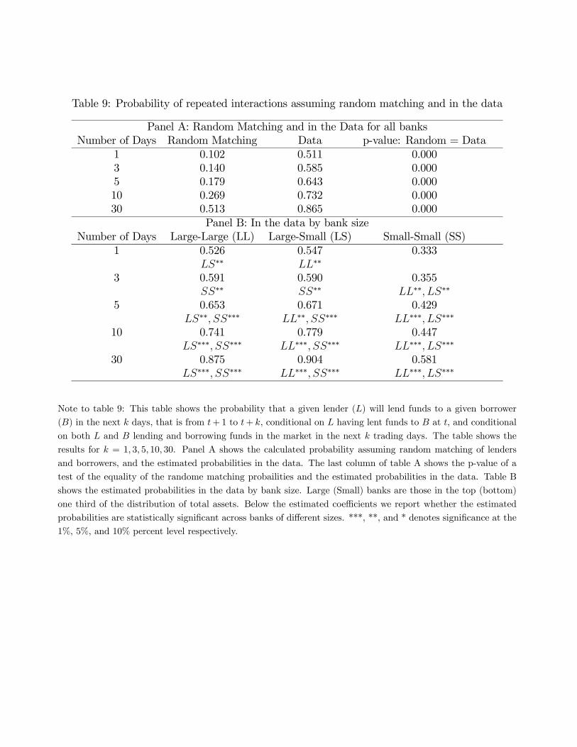
Table 9: Probability of repeated interactions assuming random matching and in the data
Panel A: Random Matching and in the Data for all banksNumber of Days Random Matching Data p-value: Random = Data
1 0.102 0.511 0.0003 0.140 0.585 0.0005 0.179 0.643 0.00010 0.269 0.732 0.00030 0.513 0.865 0.000
Panel B: In the data by bank sizeNumber of Days Large-Large (LL) Large-Small (LS) Small-Small (SS)
1 0.526 0.547 0.333LS∗∗ LL∗∗
3 0.591 0.590 0.355SS∗∗ SS∗∗ LL∗∗, LS∗∗
5 0.653 0.671 0.429LS∗∗, SS∗∗∗ LL∗∗, SS∗∗∗ LL∗∗∗, LS∗∗∗
10 0.741 0.779 0.447LS∗∗∗, SS∗∗∗ LL∗∗∗, SS∗∗∗ LL∗∗∗, LS∗∗∗
30 0.875 0.904 0.581LS∗∗∗, SS∗∗∗ LL∗∗∗, SS∗∗∗ LL∗∗∗, LS∗∗∗
Note to table 9: This table shows the probability that a given lender (L) will lend funds to a given borrower
(B) in the next k days, that is from t+1 to t+ k, conditional on L having lent funds to B at t, and conditional
on both L and B lending and borrowing funds in the market in the next k trading days. The table shows the
results for k = 1, 3, 5, 10, 30. Panel A shows the calculated probability assuming random matching of lenders
and borrowers, and the estimated probabilities in the data. The last column of table A shows the p-value of a
test of the equality of the randome matching probailities and the estimated probabilities in the data. Table B
shows the estimated probabilities in the data by bank size. Large (Small) banks are those in the top (bottom)
one third of the distribution of total assets. Below the estimated coefficients we report whether the estimated
probabilities are statistically significant across banks of different sizes. ***, **, and * denotes significance at the
1%, 5%, and 10% percent level respectively.
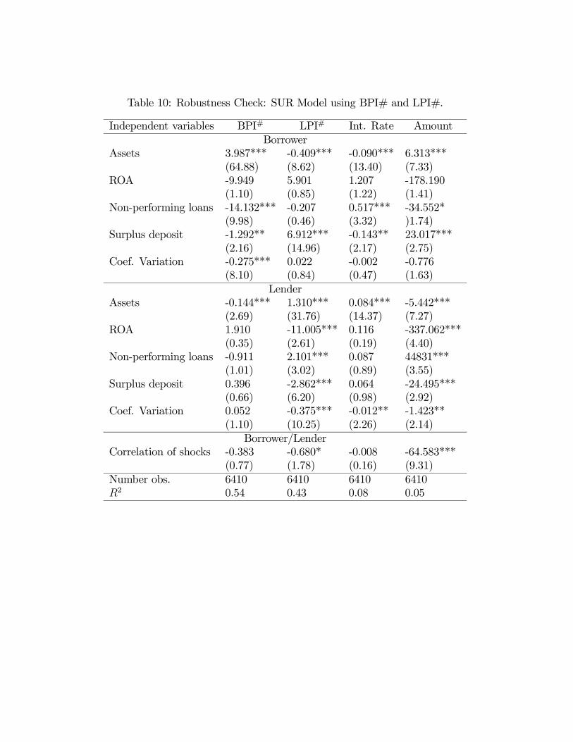
Table 10: Robustness Check: SUR Model using BPI# and LPI#.
Independent variables BPI# LPI# Int. Rate AmountBorrower
Assets 3.987*** -0.409*** -0.090*** 6.313***(64.88) (8.62) (13.40) (7.33)
ROA -9.949 5.901 1.207 -178.190(1.10) (0.85) (1.22) (1.41)
Non-performing loans -14.132*** -0.207 0.517*** -34.552*(9.98) (0.46) (3.32) )1.74)
Surplus deposit -1.292** 6.912*** -0.143** 23.017***(2.16) (14.96) (2.17) (2.75)
Coef. Variation -0.275*** 0.022 -0.002 -0.776(8.10) (0.84) (0.47) (1.63)
LenderAssets -0.144*** 1.310*** 0.084*** -5.442***
(2.69) (31.76) (14.37) (7.27)ROA 1.910 -11.005*** 0.116 -337.062***
(0.35) (2.61) (0.19) (4.40)Non-performing loans -0.911 2.101*** 0.087 44831***
(1.01) (3.02) (0.89) (3.55)Surplus deposit 0.396 -2.862*** 0.064 -24.495***
(0.66) (6.20) (0.98) (2.92)Coef. Variation 0.052 -0.375*** -0.012** -1.423**
(1.10) (10.25) (2.26) (2.14)Borrower/Lender
Correlation of shocks -0.383 -0.680* -0.008 -64.583***(0.77) (1.78) (0.16) (9.31)
Number obs. 6410 6410 6410 6410R2 0.54 0.43 0.08 0.05
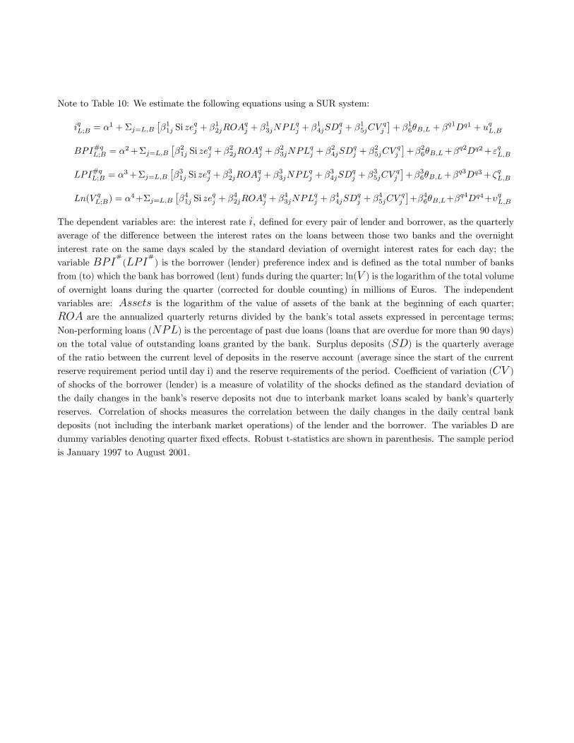
Note to Table 10: We estimate the following equations using a SUR system:
iqL;B = α1 +Σj=L,B£β11j Si ze
qj + β12jROA
qj + β13jNPLqj + β14jSD
qj + β15jCV
qj
¤+ β16θB,L + βq1Dq1 + uqL,B
BPI#qL;B = α2+Σj=L,B£β21j Si ze
qj + β22jROA
qj + β23jNPLqj + β24jSD
qj + β25jCV
qj
¤+β26θB,L+βq2Dq2+εqL,B
LPI#qL;B = α3+Σj=L,B£β31j Si ze
qj + β32jROA
qj + β33jNPLqj + β34jSD
qj + β35jCV
qj
¤+β36θB,L+βq3Dq3+ ζqL,B
Ln(V qL;B) = α4+Σj=L,B
£β41j Si ze
qj + β42jROA
qj + β43jNPLqj + β44jSD
qj + β45jCV
qj
¤+β46θB,L+β
q4Dq4+υqL,B
The dependent variables are: the interest rate i, defined for every pair of lender and borrower, as the quarterlyaverage of the difference between the interest rates on the loans between those two banks and the overnight
interest rate on the same days scaled by the standard deviation of overnight interest rates for each day; the
variable BPI#
(LPI#
) is the borrower (lender) preference index and is defined as the total number of banks
from (to) which the bank has borrowed (lent) funds during the quarter; ln(V ) is the logarithm of the total volumeof overnight loans during the quarter (corrected for double counting) in millions of Euros. The independent
variables are: Assets is the logarithm of the value of assets of the bank at the beginning of each quarter;
ROA are the annualized quarterly returns divided by the bank’s total assets expressed in percentage terms;
Non-performing loans (NPL) is the percentage of past due loans (loans that are overdue for more than 90 days)on the total value of outstanding loans granted by the bank. Surplus deposits (SD) is the quarterly averageof the ratio between the current level of deposits in the reserve account (average since the start of the current
reserve requirement period until day i) and the reserve requirements of the period. Coefficient of variation (CV )of shocks of the borrower (lender) is a measure of volatility of the shocks defined as the standard deviation of
the daily changes in the bank’s reserve deposits not due to interbank market loans scaled by bank’s quarterly
reserves. Correlation of shocks measures the correlation between the daily changes in the daily central bank
deposits (not including the interbank market operations) of the lender and the borrower. The variables D are
dummy variables denoting quarter fixed effects. Robust t-statistics are shown in parenthesis. The sample period
is January 1997 to August 2001.
Table 11: Robustness Check: Using a Two Side Relationship Metric.
Independent Two sided relationship indicesvariables BPI2 LPI2 Int. Rate Amount
BorrowerAssets -0.007*** 0.013*** -0.090*** 6.313***
(9.58) (17.61) (13.40) (7.33)ROA 0.292** -0.076 1.207 -178.190
(2.57) (0.71) (1.22) (1.41)Non-performing loans 0.035** 0.013 0.517*** -34.552*
(1.96) (0.75) (3.32) (1.74)Surplus deposits 0.013* -0.030*** -0.143** 23.017***
(1.70) (4.28) (2.17) (2.75)Coef. Variation 0.003*** -0.001 -0.002 -0.776
(7.02) (1.63) (0.47) (1.63)Lender
Assets 0.011*** -0.007*** 0.084*** -5.442***(16.88) (10.63) (14.37) (7.27)
ROA -0.050 -0.045 0.116 -337.062***(0.73) (0.70) (0.19) (4.40)
Non-performing loans 0.003 0.009 0.087 44.831***(0.29) (0.88) (0.89) (3.55)
Surplus deposits 0.006 0.002 0.064 -24.495***(0.82) (0.31) (0.98) (2.92)
Coef. Variation -0.001* 0.003*** -0.012** -1.423**(1.76) (5.10) (2.26) (2.14)Borrower/Lender
Correlation of shocks -0.067 -0.076*** -0.008 -64.583***(10.80) (12.99) (0.16) (9.31)
Number obs. 6410 6410 6410 6410R2 0.12 0.14 0.08 0.05
Note to Table 11: We estimate the following equations using a SUR system:
iqL;B = α1 +Σj=L,B£β11j Si ze
qj + β12jROA
qj + β13jNPLqj + β14jSD
qj + β15jCV
qj
¤+ β16θB,L + βq1Dq1 + uqL,B
BPI2qL;B = α2+Σj=L,B£β21j Si ze
qj + β22jROA
qj + β23jNPLqj + β24jSD
qj + β25jCV
qj
¤+β26θB,L+β
q2Dq2+εqL,B
LPI2qL;B = α3+Σj=L,B£β31j Si ze
qj + β32jROA
qj + β33jNPLqj + β34jSD
qj + β35jCV
qj
¤+β36θB,L+β
q3Dq3+ζqL,B
Ln(V qL;B) = α4+Σj=L,B
£β41j Si ze
qj + β42jROA
qj + β43jNPLqj + β44jSD
qj + β45jCV
qj
¤+β46θB,L+β
q4Dq4+υqL,B
The dependent variables are: the interest rate i,defined for every pair of lender and borrower, as the quarterlyaverage of the difference between the interest rates on the loans between those two banks and the overnight interest
rate on the same days scaled by the standard deviation of overnight interest rates for each day; BPI2 (LPI2)is the borrower (lender) preference index and is equal to the ratio of total funds that the bank has borrowed and
lent from a specific lender (borrower) as a fraction of the total amount of funds that he has borrowed and lent
in the market during a quarter; ln(V ) is the logarithm of the total volume of overnight loans during the quarter
(corrected for double counting) in millions of Euros. The independent variables are: Assets is the logarithm of
the value of assets of the bank at the end of each quarter; ROA are the annualized quarterly returns divided by
the bank’s total assets expressed in percentage terms; Non-performing loans (NPL) is the percentage of pastdue loans (loans that are overdue for more than 90 days) on the total value of outstanding loans granted by the
bank. Surplus deposits (SD) is the quarterly average of the ratio between the current level of deposits in thereserve account (average since the start of the current reserve requirement period until day i) and the reserve
requirements of the period. Coefficient of variation (CV ) of shocks of the borrower (lender) is a measure ofvolatility of the shocks defined as the standard deviation of the daily changes in the bank’s reserve deposits not
due to interbank market loans scaled by bank’s quarterly reserves. Correlation of shocks measures the correlation
between the daily changes in the daily central bank deposits (not including the interbank market operations)
of the lender and the borrower. The variables D are dummy variables denoting quarter fixed effects. Robust
t-statistics are shown in parenthesis. The sample period is January 1997 to August 2001.