learned integration of visual, vestibular, and motor cues in multiple brain regions computes head...

Learned Integration of Visual, Vestibular, and Motor Cues inMultiple Brain Regions Computes Head Direction During Visually

Guided Navigation

Bret Fortenberry, Anatoli Gorchetchnikov, and Stephen Grossberg*

ABSTRACT: Effective navigation depends upon reliable estimates ofhead direction (HD). Visual, vestibular, and outflow motor signals com-bine for this purpose in a brain system that includes dorsal tegmentalnucleus, lateral mammillary nuclei, anterior dorsal thalamic nucleus,and the postsubiculum. Learning is needed to combine such differentcues to provide reliable estimates of HD. A neural model is developedto explain how these three types of signals combine adaptively withinthe above brain regions to generate a consistent and reliable HD esti-mate, in both light and darkness, which explains the following experi-mental facts. Each HD cell is tuned to a preferred head direction. Thecell’s firing rate is maximal at the preferred direction and decreases asthe head turns from the preferred direction. The HD estimate is con-trolled by the vestibular system when visual cues are not available. Awell-established visual cue anchors the cell’s preferred direction whenthe cue is in the animal’s field of view. Distal visual cues are moreeffective than proximal cues for anchoring the preferred direction. Theintroduction of novel cues in either a novel or familiar environment cangain control over a cell’s preferred direction within minutes. Turningout the lights or removing all familiar cues does not change the cell’sfiring activity, but it may accumulate a drift in the cell’s preferred direc-tion. The anticipated time interval (ATI) of the HD estimate is greater inearly processing stages of the HD system than at later stages. The modelcontributes to an emerging unified neural model of how multiple proc-essing stages in spatial navigation, including postsubiculum head direc-tion cells, entorhinal grid cells, and hippocampal place cells, are cali-brated through learning in response to multiple types of signals as ananimal navigates in the world. VVC 2012 Wiley Periodicals, Inc.

KEY WORDS: head direction cells; learning; postsubiculum;vestibular signals; outflow motor signals; distal visual cues; spatialnavigation; visual learning; motor-vestibular calibration

INTRODUCTION

Spatial navigation is a critical means to achieve behavioral success inmany terrestrial animals. Rats use it to efficiently find food and quickly

return to a safe location. This task requires that a ratcontinuously update its current position and the direc-tion towards the safe position. A key step in this pro-cess is to estimate an animal’s direction in the envi-ronment along the entire path to the safe position.Small errors in both self-localization and directioncould accumulate over distance traveled, and therebylead the rat drastically off course. Single and multiplecell recordings in rats have produced detailed informa-tion about cells that underlie both processes: HeadDirection (HD) cells maintain directional estimates,while entorhinal grid cells and hippocampal place cellscode an animal’s position.

HD cells are found in the limbic system (Ranck,1984; Blair and Sharp, 1995; Taube, 1995; Redishet al., 1996; Stackman and Taube, 1997) and utilizeinputs from the vestibular (Blair and Sharp, 1996;Stackman and Taube, 1997; Goodridge et al., 1998),motor (Taube, 1998, 2007), and visual (Taube, 1995;Zugaro et al., 2001, 2003) systems to produce andmaintain a signal that correlates to the horizontaldirection of the head relative to the body axis.

The firing rate of a HD cell is maximal at the cell’spreferred direction and decreases as the head turnsaway from the preferred direction. There is a uniformdistribution of preferred directions among the popula-tion of HD cells (Taube, 1998). The vestibular sys-tem is the primary source of the HD signal. If thevestibular system is removed, properties of the HDcells are lost (Stackman and Taube, 1997; Taube,1998). Although the vestibular system is critical forgenerating a HD cell signal, the signal is also influ-enced by inputs from outside the vestibular system.Motor influences are revealed by experiments thatstudy the effects of passive versus active rotations(Knierim et al., 1995; Taube, 1995; Zugaro et al.,2001; Taube and Bassett, 2003). A visual landmarkcan correct the direction that has been maintained bythe vestibular and motor systems (Taube, 1995;Zugaro et al., 2001, 2003, 2004; Yoganarasimhaet al., 2006).

The activity of HD cells anticipates the directionthat is assumed by the rat’s head during head rota-tions. The timing of this anticipation is referred to asthe anticipatory time interval (ATI), and is observedin the lateral mammillary nuclei and anterior dorsalthalamic nuclei. It has been theorized that the antici-

Center for Adaptive Systems, Department of Cognitive and Neural Sys-tems, and Center of Excellence for Learning in Education, Boston Uni-versity, Boston, MassachusettsGrant sponsor: CELEST, an NSF Science of Learning Center; Grant num-ber: SBE-0354378; Grant sponsor: SyNAPSE program of the DefenseAdvanced Research Projects Agency; Grant number: HR0011-09-C-0001.*Correspondence to: Stephen Grossberg, Center for Adaptive Systems,Department of Cognitive and Neural Systems And Center of Excellencefor Learning in Education, Science and Technology Boston University,677 Beacon St, Boston, MA 02215. E-mail: [email protected] for publication 16 April 2012DOI 10.1002/hipo.22040Published online in Wiley Online Library (wileyonlinelibrary.com).

HIPPOCAMPUS 00:000–000 (2012)

VVC 2012 WILEY PERIODICALS, INC.

pation is due to motor and vestibular system interactions (Blairand Sharp, 1995; Stackman and Taube, 1997). Indeed, the ATIis greater during passive rotations than active rotations (Bassettet al., 2005).

Rate-based and spiking models have been developed toexplain how HD cell responses can be generated and main-tained using vestibular angular head velocity inputs (Blair andSharp, 1995, 1996; Redish et al., 1996; Goodridge and Tour-etzky, 2000; Boucheny et al., 2005; Song and Wang, 2005).These models have demonstrated accurate and robust HDresponses during head rotations. Some of the models also sug-gested how visual cues may influence the HD signal. All thesemodels used simple structures with only a few of the regionsknown to contain HD cells. They have not addressed howthese circuits adaptively calibrate vestibular, motor, and visualsignals to generate consistent commands in the multistage braincircuits that carry out HD computation, how different timingrates occur in the two brain hemispheres during a head rota-tion, and how motor inputs can contribute to the ATI effect.

In this paper, a neural model, called the HeadMoVVes(Head direction from Motor, Visual, and Vestibular signals)model, is developed to explain how vestibular, motor, and vis-ual cues combine through learned interactions to generate aconsistent and reliable HD estimate, under light or dark con-ditions, and to explain the following types of data: howmotor and vestibular system interactions can produce an ATIshift, why ATI shifts differ for clockwise and counter-clock-wise head rotations, why so many regions in the limbic sys-tem contain HD cells, why simpler circuitry cannot accom-plish these tasks, how visual landmarks reset the HD cell’spreferred direction, and why distal landmarks have a strongereffect on the firing properties of HD cells than proximallandmarks. These results have been briefly reported in Forten-berry et al. (2009a,b).

MATERIALS AND METHODS

This section summarizes experimental data about the proper-ties of head direction (HD) cells, previous ring attractor modelsof HD cells, and the HeadMoVVes ring attractor model that isused to explain and simulate key experimental data.

Experimental Properties of Head Direction Cells

Directional tuning

HD cells are characterized by their tuning curve during a3608 rotation. Cell firing is maximal at the preferred directionand decreases as the head rotates in either direction away fromthe preferred direction (Fig. 1). The tuning curve can eitherhave a triangular, cosine or Gaussian shape (Blair and Sharp,1995; Taube, 1995). The cell is defined by the preferred firingdirection, peak firing rate, tuning curve width, and baseline fir-ing, which is at or near zero for most cells (Taube, 1998). Thetuning curve width varies with brain region from 608 to 1508at base rate. The peak-firing rate also depends on brain regionand can range from 16 (spikes/s) to 120 (spikes/s) (Taube andBassett, 2003). The cell’s preferred direction is influenced bythe vestibular, motor, and visual systems. When visual input isnot available, the vestibular and motor systems sustain HD ac-tivity but may accumulate a slow drift of the preferred direc-tion (Knierim et al., 1998). However, a well-established visualcue can reset the preferred direction and consistently anchor itto a landmark (Taube, 1995; Zugaro et al., 2001, 2003, 2004;Yoganarasimha et al., 2006).

Hemispheric differences in HD cells

The HD system in rats receives angular head velocity (AHV)input from the nucleus prepositus hypoglossi (PPH) and the

FIGURE 1. Time slide analysis on a population of angularhead velocity (AHV) cells in the left hemisphere. The activitybelow baseline occurs during periods preceding a head rotationand the activity above baseline occurs during periods succeeding ahead rotation. The ipsiversive hemisphere (counter–clockwise)

anticipates the head rotation while the contraversive hemisphere(clockwise) is delayed. The HeadMoVVes model assumes that thedifferences are due to motor and vestibular AHV inputs, respec-tively. [Reprinted with permission from Sharp (2001)]

2 FORTENBERRY ET AL.

Hippocampus

medial vestibular nucleus (MVN), which project to the dorsaltegmental nucleus (DTN). The DTN contains both AHV cellsand AHV-HD combination cells (Stackman and Taube, 1997;Blair 1998; Taube, 1998). Sharp et al. (2001) analyzed the tim-ing of AHV cell activation in the DTN in the two hemispheresin response to head rotations in both the clockwise and coun-ter-clockwise directions. Their time slide analysis correlates thefiring rate of the AHV cells to the rat’s head rotation for recentpast, present, and near future. Cell activity is measured in16.7-ms intervals from 1,000 ms prior to a head rotation to1,000 ms after a head rotation. Figure 1 shows the result ofaveraging a population of cells in the left hemisphere for bothclockwise and counter-clockwise time slide correlates acrossfour consecutive samples of head rotations in the left hemi-spheres with a minimum turning rate of 250 deg/s. The twocurves represent two different directions of head movements.During a clockwise rotation, the left hemisphere is the contra-versive hemisphere. During a counter-clockwise rotation, theleft hemisphere is the ipsiversive hemisphere (Fig. 1). TheAHV signal in the contraversive hemisphere during a clockwiserotation lags until after the head rotation. The AHV signal inthe ipsiversive hemisphere during a counter-clockwise rotationpeaks prior to the head rotation.

The HeadMoVVes model assumes that AHV cell activationobeys the same laws for clockwise and counter-clockwise headmovements in both hemispheres of the DTN. The data for theright hemisphere in Sharp et al. (2001, Fig. 7, middle panel)show a similar qualitative effect as in the left hemisphere, butthe counterclockwise peak is attenuated. Moreover, this trendcontinues to be seen, although weaker than for the left hemi-sphere alone, in the combined hemisphere data (Fig. 7, bottompanel). Currently, the reason for this asymmetric activation isunclear. Additional data would be welcome to clarify its basis.For simplicity, the model currently assumes symmetric activa-tion if only because clockwise and counterclockwise rotationsof the head both occur, and the most parsimonious design isone that would regulate them in a similar way acrosshemispheres.

Two types of inputs: Vestibular andmotor outflow

The types of cells found in the DTN can explain the timingeffects found in the time slide analysis. The PPH of the vestib-ular system contains two types of inputs based on different haircells in the semicircular canal. Type I cells respond to ipsiver-sive head rotations and Type II cells respond to contraversivehead rotations (Gdowski and McCrea, 2000; Klam and Graf,2003). The PPH contains about twice as many Type II thanType I vestibular neurons (Blair et al., 1998; Lannnou et al.,1984). The DTN, in turn, receives vestibular information fromthe PPH. Thus, it is reasonable to assume that delayed AHVsignals to the contraversive hemisphere of the DTN are drivenby Type II vestibular neurons, while anticipatory signals to theDTN ipsiversive hemisphere are driven by another source. TheHeadMoVVes model uses motor outflow in the ipsiversive

hemisphere and does not address the functional role that TypeI vestibular neurons may have.

This source is herein assumed to be motor outflow, or corol-lary discharge, signals. The interpeduncular nucleus (IPN) hasbeen implicated as a possible source of motor outflow signalsto the DTN (Sharp et al., 2006; Taube et al., 2009). The IPNhas reciprocal connections to the DTN and has neurons sensi-tive to movement speed. Lesions of the IPN (Taube et al.,2009) attenuate the preferred direction firing rate in ADN HDneurons. Passive head rotations without motor signals have aless clear effect on cell firing rates. Some older studies (Knierimet al., 1995; Taube et al., 1990; 1995) suggested that the firingrates are attenuated, while more recent data by Shinder andTaube (2011) suggest that there is no attenuation of firing ratein the case of passive rotations.

Region-specific properties of HD cells

Most HD cells are found in lateral mammillary nuclei(LMN), anterior dorsal thalamic nucleus (ADN), postsubicu-lum (PoS), and retrosplenial cortex (RSC); see Figure 2. HDcells are also found in the entorhinal cortex (Sargolini et al.,2006) but these cells are downstream from the circuit describedhere. HD cells are found in both hemispheres and complex cir-cuitry connects the associated regions. The PoS, which appearsto be the final stage containing pure HD cells, projects into theentorhinal cortex where some pure HD cells are mixed withconjunctive cells that extend HD with spatial properties thathave been proposed to help create positional maps for guidingspatial navigation (Fuhs and Touretzky 2006; Burgess et al,2007; Mhatre et al., 2012; Pilly and Grossberg, 2012). Bilaterallesions in the LMN or DTN quench HD cells in the ADN(Blair et al., 1998; Bassett et al., 2007) and PoS (Sharp et al.,2006); see Figure 2. Unilateral LMN lesions do not eliminatethe HD cell properties in either the ADN or PoS (Blair et al.,1999). Lesions in the ADN disrupt the HD properties in thePoS (Goodridge and Taube, 1997). The PoS also receives inputfrom visual regions (Vogt and Miller, 1983; Taube, 1998) andis a good candidate for vision-driven HD preferred directionresets.

Anticipated time interval

As noted above, HD activity in the LMN and ADN antici-pates the rat’s head rotation (Blair and Sharp, 1995). Thisanticipated time interval (ATI) is more prominent in the LMN(�70 ms), reduced in the ADN (�25 ms), and disappears inthe PoS (Sharp et al., 2001; Taube, 1998, 2007). It has beentheorized that the properties of the ATI are due to motor andvestibular system interactions (Taube and Muller, 1997). In theLMN, the recordings from the ipsiversive hemisphere (thehemisphere towards which the head is rotating) showed a largerATI than the recordings from the contraversive hemisphere,but in the ADN, the ATI was the same in both hemispheresfor ipsiversive and contraversive head turns (Blair et al., 1998).

ADAPTIVE CALIBRATION OF HEAD DIRECTION 3

Hippocampus

Ring Attractor Models of Head Direction

Ring attractors have been widely used to computationallymodel HD cells (Blair and Sharp, 1995, 1996; Skaggs et al.,1995; Redish et al., 1996; Goodridge and Touretzky, 2000;Boucheny et al., 2005; Song and Wang, 2005). Such ringattractors use a circular recurrently connected network with dy-namics which produce an activity bump whose position in thering represents head direction. Properties of this HD bump arethen compared with the firing characteristics observed in HDcell recordings. Integration of angular head velocity (AHV) sig-nals shifts the activity bump around the ring. The recurrentconnections in the ring attractor can be implemented usingconnections between the dorsal thalamic nucleus (DTN) andthe lateral mammillary nucleus (LMN) (Blair et al., 1998;Song and Wang, 2005) using inhibitory connections fromDTN to LMN and excitatory connections from LMN to DTN(Fig. 2).

In HD ring attractors, vestibular AHV inputs control thedirection and speed of the activity bump shift to match therotation of the head. Because vestibular AHV input is a delayedsignal, it does not explain the anticipatory shift found in the

LMN and ADN. Previous ring attractor models have proposeddifferent mechanisms to explain this anticipatory shift. Thesemechanisms and their corresponding models are summarized inthe Discussion section. As noted above, the HeadMoVVesmodel proposes that motor outflow signals produce anticipa-tion. The model then needs to clarify how the brain adaptivelycalibrates visual, vestibular, and motor cues to become dimen-sionally consistent. To accomplish this, the model proposeshow multiple brain regions contribute to the calibrationprocess.

Model Overview

The HeadMoVVes model was tested using a computer simu-lation of HD cell responses while a virtual artificial animal, oranimat, navigates a square environment in which visual land-marks occur in proximal and distal locations. The model HDsystem was also implemented in a physical robot to demon-strate its capabilities (Fortenberry et al., 2011), but this applica-tion is beyond the scope of this article.

In the model, head turns are simulated with different accel-erations and durations of rotation. A Gaussian profile of the

FIGURE 2. HeadMoVVes model functions [left column] andmacrocircuit [right column]. The HeadMoVVes model requires themultiregion circuitry to adaptively calibrate motor, vestibular, andvisual signals into a reliable HD estimate. AHV, angular head ve-locity; DTN, dorsal tegmental nucleus; LMN, lateral mammillarynuclei; ADN, anterior dorsal thalamic nucleus; PoS, postsubicu-

lum; RSC, retrosplenial cortex; EC, enthorhinal cortex. Blackarrowheads are excitatory connections, hemi-disks are adaptiveconnections, and circles are inhibitory connections. The labels inthe top right of each brain region and letters along the connec-tions refer to the variables and weights in the Appendix mathe-matical equations.


Hippocampus

AHV input through time is produced with amplitudes ran-domly chosen between 2.5 and 2.9, which equate to 2502290deg/s, that determines the speed of a head rotation, and a headturn duration of 220–280 ms. Figure 3 shows an example ofthe input amplitude set to 2.6 with duration of 260 ms. Thetime intervals in the simulations are computed with respect tothe durations of head rotations taken from the data of Sharp(2001). In Figure 3, the actual head rotation (solid line) isplotted against time in 10 ms time steps and is shown with themotor AHV input that is shifted 25 ms earlier in time thanthe head rotation (dotted line) and the vestibular AHV inputthat is shifted 25 ms later in time than the head rotation(dash-dotted line) signals. Noise is added to the motor and ves-tibular AHV signals to model neuronal and synaptic noise. Themotor and vestibular AHV signals are sent to the DTN layerof the ring attractor (Fig. 2) and the true head velocity is usedto rotate the animat every 10 ms.

Dual hemisphere calibration

The HeadMoVVes model uses a two hemisphere systemwhere one hemisphere receives a motor outflow anticipatoryAHV input and the other receives a vestibular delayed AHVsignal in response to each head rotation. The dual hemispherecalibration allows the system to predict the true head positionduring a turn despite the time difference between these twoinputs. To accomplish this, several brain regions process the in-formation in sequence, each having a different function, so thatthe last HD region, the PoS, produces the correct timing(Fig. 2). The DTN and the LMN convert vestibular and motorAHV into a HD signal. The ADN combines the motor andvestibular HD estimates from the LMNs in both hemispheres

(Fig. 2). The PoS estimates a single HD estimate by combininginformation across both hemispheres. The visual input pro-vided to PoS is used as a final error correction signal thatanchors the internally driven HD estimate to visual landmarks.The visual, vestibular, and motor outflow signals hereby worktogether to increase the reliability of the HD estimate.

Automatic gain control using habituative gates

Vestibular and motor inputs may activate their target cellswith different gains. The signal strengths of corresponding motorand vestibular angular velocities must match to produce compa-rable HD direction shifts for the dual hemisphere interaction towork correctly. Then the two hemispheres can converge to thesame output independently of which input drives them. Howare these inputs adaptively calibrated to enable successful match-ing to occur? A habituative gating mechanism [Appendix Eqs.(A4) and (A5)] is proposed to accomplish this. Such a gatingprocess in each input pathway time-averages motor and vestibu-lar inputs over a long time scale and normalizes the input signalsin its pathway with this time-averaged value, much as happensin retinal photoreceptors (Carpenter and Grossberg, 1981;Grossberg and Hong, 2006), cortical motion perception circuits(Baloch and Grossberg, 1997; Berzhanskaya et al., 2007), andamygdala reinforcement learning circuits (Grossberg, 1972; Dra-nias et al., 2008), among other brain systems. As both motorand vestibular inputs become normalized, the signal strengths ofvestibular and motor inputs can produce matching signals duringhead rotations with variable speeds and distances.

Ring attractors in the DTN and LMN

Two ring attractors, one in each hemisphere, are used to pro-duce the head direction representation from motor and vestibu-lar AHV inputs. The position of an activity bump representsthe head direction at any time. Interactions between the dorsaltegmental nucleus (DTN) and lateral mammillary nuclei(LMN) define each ring attractor (Figs. 2 and 4). Each hemi-sphere contains two DTN layers and one LMN layer [Appen-dix Eqs. (A6)–(A12)]. One DTN layer receives vestibular AHVinput and the other receives motor AHV input. The vestibularAHV input produces a shift of the activity bump in the direc-tion opposite to the hemisphere of the attractor (left shift forthe right hemisphere and right shift for the left hemisphere).The motor AHV produces a shift of the bump in the directionthat matches the hemisphere of the attractor. In particular,motor AHV input to the right hemisphere causes the ringattractor in the right hemisphere to shift its bump to the right,whereas vestibular AHV input to the left hemisphere causes thering attractor in the left hemisphere to also shift its bump tothe right. Although both ring attractors shift to the right, theshift due to input from the right hemisphere precedes the headrotation, whereas the shift due to input from left hemisphere isdelayed. During a left head rotation, the situation is reversed.

The connections in the ring attractor that produce the activ-ity bumps and their shifts in response to motor and vestibularAHV inputs are asymmetric inhibitory connections from each

FIGURE 3. The angular head velocity (AHV) curves and tim-ing for the HeaDMoVVes model inputs. The motor AHV (dashedline) curve is the input to the ipsiversive hemisphere, the vestibularAHV (dash-dotted line) curve is the input to the contraversivehemisphere, and the head (solid line) curve is the velocity of theanimat’s head movement. The x-axis shows the angular velocity forone time step and each simulation time step corresponds to 10 msin duration.


Hippocampus

DTN layer to the LMN layer, with the direction of the asym-metry opposite for the two DTN layers, and symmetric excita-tory feedback connections from the LTM to both DTN layers(Fig. 4). The DTN layers also have symmetric recurrent inhibi-tory connections centered on DTN cells that are 1808 awayfrom the source of the connection to sharpen and stabilize thebump. All three layers continuously receive Poisson-distributedinputs that determine a baseline of activity.

The LMN-to-DTN excitatory projection connects LMN andDTN cells that represent the same head direction. A bump inthe LMN hereby produces a bump in the same position in

both DTN layers. The DTN inputs equally inhibit the sides ofthe LMN bump when the head is motionless. A head rotationsends either motor or vestibular angular velocity input to oneDTN layer, increasing the asymmetrical inhibition in onedirection, and shifts the ring in the direction with less inhibi-tion. The speed of the shift is proportional to the difference ofinhibitory input from the two asymmetrical connections.

Anterior dorsal thalamic nuclei

The ADN combines the LMN HD estimates from the twohemispheres to produce a HD estimate that has more precisetiming than one that depends only on one of the motor or ves-tibular inputs [Fig. 2; Appendix Eqs. (A13)–(A14)]. The motor-driven ipsiversive LMN estimate is anticipatory, but the vestibu-lar-driven contraversive LMN estimate is delayed for each headrotation. The ADN activity adds the two LMN signals to createan activity bump in the position that is an average of the twoLMN estimates. Adjusting the gain parameter F [see AppendixEqs. (A13) and (A14)] between 0 and 1 adjusts the gain fromthe contralateral LMN and affects the amount of anticipationfound in the ADN. The sigmoidal signal function from theLMN-to-ADN [Appendix Eq. (A15)] positionally sharpens theresulting bump and creates an ADN signal that is narrower thaneach of the LMN signals. The comparison of HD estimates inthe LMN and ADN of the model with the experimental datashows correspondence of a signal profile and ATI (see Fig. 9below).

Post subiculum: Dual hemisphere competition

The ADN sends one-to-one topography-preserving connec-tions to the PoS, as shown in Figure 5. The PoS makes directexcitatory connections and indirect inhibitory connections viainhibitory interneurons with the contralateral PoS. These con-nections together form a center-surround network with a nar-

FIGURE 4. Microcircuit of the DTN-LMN ring attractor. TwoDTN regions and one LMN region interact to form a ring attrac-tor. The inhibitory and excitatory connections between the threelayers create a single activity bump that spans multiple cells. Thetwo DTNs receive angular head velocity (AHV) inputs. The inhibi-tory connections from the two DTNs to the LMN are shifted toopposite directions. When the two inputs differ, the inhibitory off-set causes the position of the activity bump the represents headdirection to shift in the direction away from that of the larger in-hibitory input.

FIGURE 5. Microcircuit of the ADN to PoS connections.These connections embody the PoS competition. The PoS (PL,PR) in each hemisphere (L, R) receives a one-to-one excitatoryconnection from the corresponding ADN (AL, AR) cell. During ahead rotation, the HD direction in each hemisphere differs. The

excitatory (WppEx) and inhibitory (WppIn) interactions form arecurrent on-center off-surround network that forces the two PoSHD estimates to compete and merge the two ADN estimates toone position.


Hippocampus

row strong on-center and a broad weak off-surround [AppendixEqs. (A16) and (A17)]. The two reciprocally interacting center-surrounds, one in each hemisphere, drive the HD estimates inthe two PoS hemispheres to the same position.

Retrosplenial cortex: Visual landmarks

Vestibular and motor signals alone are not sufficient to esti-mate the true head position over time. Visual inputs to the PoS(Fig. 2) anchor and stabilize the HD cell’s preferred direction tothe environment [Appendix Eqs. (A18)–(A20)]. Adding visualinputs to the model needs to take account of the fact that a sin-gle visual cue can match different HD estimates depending onthe position of the rat in the environment. For example, if alandmark is positioned in the middle of the north wall of theenvironment and a rat is facing north, the landmark will appearin the rat’s right hemifield if the rat is next to the west wall andin the left hemifield if the rat is next to the east wall.

The model learns a mapping between visual landmarks andthe HD estimate in the PoS. To be able to discriminatebetween different positions of the animal when a landmark isviewed, the model contains ‘‘object-in-place’’ cells that conjunc-tively fuse information about objects and their positions in theenvironment. These cells are organized in object-place hyper-columns. Each hypercolumn responds to a unique object andeach cell within the hypercolumn responds to a unique head-centric spatial position of the object in the horizontal plane.Such a conjunctive representation of visual features and posi-tions is found in the rat brain in areas such as the retrosplenialcortex (RSC) (Vann, 2009). The RSC receives connectionsfrom cortical area V1 (Wang and Burkhalter, 2007) and theparietal cortex (Taube, 1998). The RSC connects to the ADNand the PoS (Van Groen and Wyss, 1992, 2003; Taube, 2007)and contains HD cells (Chen et al., 1994; Cho and Sharp,2001). The HeaDMoVVes model does not address the RSC-to-ADN connection because the functional role of this connec-tion is not clear, although the model RSC does project indi-rectly to the ADN via the PoS and LMN (Fig. 2). Lesions inthe RSC produce less stable HD cells whose directional selec-tivity can drift over time (Clark et al., 2010). A similar driftcan also occur during navigation with the lights turned off(Knierim et al., 1998). The model also predicts that RSClesions will have a similar effect on LMN and ADN cells dueto the projection of RSC to these areas via the PoS.

Each visual layer in the model contains 20 cells, where eachcell represents 108 of visual angle. Each landmark activates twoto three RSC cells with a strength that falls off with distancefrom the landmark position [Appendix Eq. (A18)]. The com-bined visual span of all the cells is 200 degrees (Fig. 6). Whena visual landmark appears in a prescribed position and the cor-responding cells activate, the adaptive weights from the RSC tothe PoS [Appendix Eq. (A19)] learn the mapping between theposition of the landmark and the current HD estimate in thePoS. The adaptive weights are initialized to zero to learn anovel environment. The vision cells start to affect the HD esti-mate in the PoS as the weights are established through learning.

When a vision cell is active, the weights increase if the PoS cellis active but decrease if the PoS cell is silent. Over time thelandmarks that are more stable result in a stronger connection(see Fig. 11 in the Results section). Distal landmarks learn toinfluence the PoS more than proximal landmarks, as in thedata (Taube, 1995; Zugaro et al., 2001, 2003, 2004; Yoganara-simha et al., 2006), because the relative positions of distal land-marks as the rat moves are more consistent over time.

For a landmark to predict head direction the relative position ofthe landmark must statistically have more movement when the rat’shead rotates than when the rat maintains the same head directionbut shifts to different positions in the environment. The statisticsare determined by the distance to the landmark and the size of theenvironment. As the size of the environment increases, the land-marks must be more distal to ensure that the movement of thelandmark is a statistically stronger representation of head rotationsrather than the rat’s position in the environment. This article fixesthe size of the environment and analyzes the effect the landmarkdistance has on the stability of head direction signal.

RESULTS

General Setup for Simulations With Vision

The simulated environment is a square enclosure with visuallandmarks placed either far from (distal) or close to (proximal)

FIGURE 6. The arrangement of the visual cues in the environ-ment. The animat is confined to the inside of the box. The rowsof circles on the bottom represent the different visually activatedobject hypercolumns. Each visual cue activates a position in itshypercolumn when it is in the FOV. Activation strength is repre-sented by an inverse grayscale intensity where white is zeroactivation.


Hippocampus

the enclosure (Fig. 7). The animat moves within the enclosure,turning a random direction every 2–5 s. The animat moves for-ward at a constant speed while rotating unless it runs into awall. When the animat hits a wall it rotates until it can runalong the wall. Landmarks are positioned at variable distancesin a 3608 circumference, strategically placed to reproduce thedata of Zugaro (2004) using the landmark distribution that isdescribed in the next section. For simplicity, the animat’s eyesin the simulations were fixed in the head. As a result, land-marks were directly viewed in head-centric coordinates, therebyeliminating the need to transform visual inputs from retinalcoordinates into head-centric coordinates that is necessary incase of moveable eyes.

Habituative gates

Vestibular and motor AHV inputs may differ in strength, forthe same movements, if only because the inputs are producedin different regions of the brain. As noted above, the modeluses habituative gates to transform vestibular and motor AHVinputs into signals that have similar average gains, and that canthus be matched in a consistent way. To test the performanceof the habituative gates, three simulations were performed withthe motor AHV inputs set to 0.7, 1.3, and 1.8 times that ofthe vestibular inputs and constant throughout a trial. The ves-tibular AHV and head rotation curves were produced as speci-fied in Figure 2. All learning trials begun with all the motorand vestibular habituative gates set initially to one, which is the

gate equilibrium value before inputs occur [Eq. (5); AppendixTable A2], and go through a training stage and testing stage.Training involves the animat moving randomly through theenvironment while constantly changing direction as in a ran-dom foraging task. Learning occurs until the habituative gatevalues stabilize. Vision was turned off during the training pe-riod in the simulations presented here to study the direct effectof habituative adaptation without the visual landmark correc-tion to the PoS. This is not required though, and visual learn-ing can go on continuously even while habituation is occurringbecause the habituation does not sense the effects of vision, butrather enables visual learning to stabilize after habituation sta-bilizes. After learning has been established, the performance ofthe model with habituative gates was tested and compared withthe performance of the model without habituative gates.

The habituative gates can take as long as 1,000 head rota-tions to stabilize. The HD estimate in the PoS will not matchthe animat’s head rotation until the habituative gates are stabi-lized. Figure 8 describes the results of a simulation of habitua-tive gate gain adjustment for a motor AHV gain of 0.7 timesand 1.8 times the vestibular AHV gain in parts (A) and (B),respectively. Part (A) shows the motor habituative gate stabiliz-ing near 0.5 to match the vestibular AHV gain. Part (B) showsthat the motor habituative gate stabilizes near 0.2 to decreasethe motor AHV gain to match the vestibular AHV gain. Inboth instances the vestibular habituative gates stabilize near0.38.

Postsubiculum and ATI

As noted above, HD activity in the LMN and ADN antici-pates the rat’s head rotation (Blair and Sharp, 1995). Thisanticipated time interval (ATI) is more prominent in the LMN(�70 ms), reduced in the ADN (�25 ms), and disappears inthe PoS (Sharp et al., 2001; Taube, 1998, 2007). It has beentheorized that the properties of the ATI are due to motor andvestibular system interactions (Taube and Muller, 1997). In theLMN, the recordings from the ipsiversive hemisphere (thehemisphere towards which the head is rotating) showed a largerATI than the recordings from the contraversive hemisphere,but in the ADN, the ATI was the same for ipsiversive and con-traversive head turns (Blair et al., 1998).

In the model, the postsubiculum (PoS) competition resultsin the final elimination of the ATI and enables the HD esti-mate to match the animat’s head rotation. The competitionincludes activity in both hemispheres and visual input (Fig. 2).To test this effect, a complete head rotation was plotted fromthree trials, the first with neither the PoS competition norvision, the second with the PoS competition but withoutvision, and the third with both PoS competition and vision.The two trials without vision took place in a novel environ-ment without visual landmarks. The trial with vision used sixdistal landmarks.

The visually activated adaptive weights are large enough toinfluence a shift after eight minutes of learning, but learningcontinued after that at a rate dependent on how often the vis-

FIGURE 7. The environment for the proximal-distal landmarkconflict shift study. The animat randomly moves within the graysquare enclosure during the entire study. After the animat learnsthe environment, the proximal and distal landmarks are rotated908 in different directions to determine which landmark the HDestimate follows. A trial is recorded as a distal shift when the HDestimate shifts between 70 and 1108, a proximal shift when theHD estimate shifts between 270 and 21108, or a mixed shiftwhen the HD estimate shifts less than 208 or more than 1608 ineither direction. The gray areas show the regions that constitute adistal, proximal, or mixed shift in HD estimate when the animat’soriginal position is facing down.


Hippocampus

ual landmarks were viewed. Training took place for 30 min toensure all the landmarks established strong learning curves.

Three plots were produced to show the effect of PoS compe-tition, with and without vision (Fig. 9). Without PoS competi-

tion, the PoS layers track the ADN layers from the same hemi-sphere. In particular, the ipsiversive PoS (dashed line) tracks theipsiversive ADN (triangle line), while the contraversive PoS(small dotted line) tracks the contraversive ADN (big dotted

FIGURE 8. The performance of the habituative gates. The leftcolumn describes the vestibular input (v), its habituative gate (zv),the gated vestibular input (Hv) to the DTN layer of the two ringattractors. The right column describes the corresponding quanti-ties for the motor input. Although the vestibular and motor inputs

are significantly different, their gated inputs have a normalizedgain that enables them to be matched. (A) The effect of the habit-uative gates when the motor gain is smaller than the vestibulargain. (B) The effect of the habituative gates when the motor gainis larger than the vestibular gain.


Hippocampus

line) (Figs. 9A,D). When the PoS competition is turned on,the two PoS hemispheres merge towards one another to a posi-tion near the ipsiversive ADN (Figs. 9B,E). The model predicts

that lesioning cross-hemispheric interaction within the PoSshould lead to disagreement in HD estimates between the twoPoS hemispheres, especially during rotation. This type of lesionwill cause the PoS cells to behave more like anticipatory ADNcells. When visual input is available, the two PoS hemispheres(small dotted line and dashed line) track the animat’s rotationand are no longer anticipatory. In Figures 9B,E, without visualinput from RSC, the two PoS hemispheres are aligned to theipsiversive ADN, but in Figures 9C,F, with visual input fromRSC, the two PoS hemispheres are aligned with the animat’shead position (solid line). Thus the model predicts that, with-out visual input, the activity in the two PoS hemispheres willalign but will anticipate the head rotation.

HD visual reset

Both visual inputs via the RSC and vestibular/motor inputsvia the ADN influence the PoS competition (Fig. 2). Visuallandmarks are anchored to the environment while AHV inputsfluctuate with the dynamic HD estimates in the previous timestep. As a result, the HD estimate in PoS will continually shifttowards the visually guided position. This process occurs within10–20 ms and often appears on the coarse plots as an immedi-ate jump to the visually guided position. This shift is relayedback to the LMN through the PoS-to-LMN feedback connec-tion (Fig. 2). If two landmarks within the visual field areincongruent, the shift will follow the landmark with the stron-ger learned weights. If only one landmark is present in the vis-ual field, the shift will tend to follow that landmark even if itis a weak landmark. The number of landmarks, the strength oflearned weights, and how long each landmark is in the visualfield together determine the speed of visual correction of theHD estimate. The following sections summarize simulations ofthe effects of visual cues under different circumstances.

HD estimate drift without vision

There is some evidence of a HD drift when an animal navi-gates in the dark (Knierim et al., 1998). The drift is often lessthan 458 but can drift >908 when the lights are off for morethan 3 min. The drift will show variability and drift back andforth to maintain a drift <458 before drifting to greater distan-ces. We tested if the model produced a HD drift when visionwas not available. To test this, the difference between the HDestimate and the animat’s head position was measured every 20s for 30 min. Given that a head rotation occurs every 2–5 s,the animat has �5.5 head rotations every 20 s. Forty trialswere run with 20 vision trials and 20 nonvision trials. Thehead turn direction was randomly selected, which led to rota-tions in both the clockwise and counter-clockwise direction butcould have consecutive head rotations in the same direction.The trials with and without vision followed the same paradigmas the PoS competition trials described in the previous section.

The HeadMoVVes model is reliable without vision and canrun for hours with only modest drifts occurring. In particular,out of 20 nonvision trials, 50% drifted less than 108, and 95%drifted less than 208. In one trial the drift did reach 408 as

FIGURE 9. The effect of the PoS competition. The graphsshow the timing of a rotation for both hemispheres of the ADNand PoS in comparison to the animat’s head rotation (solid blackline). All lines to the left of the solid black line are anticipatoryand all lines to the right are delayed. The left side of each image isthe complete head rotation and the right is a 50 ms magnifiedwindow. [A, D] is the effect without PoS competition. [D] the PoStracks the ADN without PoS competition. [B,E] is the effect ofPoS competition without visual input from the RSC. [E] the PoScurves merge towards the same position between. [C, F] the effectof PoS competition with vision input from the RSC. [F] the twoPoS curves tracking the position of the animat’s head rotation andare no longer anticipatory.


Hippocampus

seen in Figure 10. All vision trials showed drifts that were lessthan 88 of the true head position (Fig. 10).

Proximal and distal visual landmarkdiscrimination task

Zugaro et al. (2004) designed a task to show that the HDdirection follows distal rather than proximal landmarks whenthese cues rotate in opposite directions. The Zugaro study usedtwo landmarks placed at different distances that rotated inopposite directions. Landmark size was chosen so that objectsappeared the same size in the rat’s field of view to avoid sali-ency preferences during learning.

In model simulations, five trials were run with the landmarksplaced at different distances. All landmarks were given thesame size and saliency on the retina for all distances to avoidbiases during learning. The general layout of the trials can beseen in Figure 7. All trials set the proximal and distal land-marks at the same relative distances (1:4) as the Zugaro et al.study but at different absolute distances to test the distanceeffect of the proximal landmark. The distances of (proximal,distal) landmarks are specified by Euclidean distance in pixelsfrom the center of the enclosure. Proximal and distal landmarksin the first two trials were (50, 200) and (100, 400) pixelsfrom the center of the enclosure, with the proximal landmarkpositioned inside the enclosure. The third trial, with landmarksat (150, 600) pixels from the center of the enclosure, posi-tioned the proximal landmark just outside the enclosure. Thelast trial, with landmarks at (300, 1,200) pixels from the centerof the enclosure, positioned the proximal landmark significantlyoutside the enclosure. The hypothesis is that closer proximallandmarks have less influence on the HD cell’s preferred direc-tion. Keeping the same ratio ensures that moving the proximallandmark does not change the relative proximity of the twolandmarks.

For each trial, the animat is trained for thirty minutes, whichis a sufficient duration to establish strong visual learning, beforethree measurements were taken of the PoS HD estimate. Theleft hemisphere PoS HD estimate was arbitrarily used for alltrials because each PoS estimate produces the same position.The HD estimate is measured prior to a landmark shift inorder to determine the initial position of the HD estimate.Then the proximal and distal landmarks were rotated 908 inopposite directions. After one second a new PoS HD estimateis measured. This second measurement determined the amountof shift from the first recording. The landmarks were thenrotated back to the original position and, after one more sec-ond, a third PoS HD estimate was measured. The third HDestimate measurement determined the shift accuracy. After thisthird measurement, the initially learned weights were reinstatedto overcome any partial learning due to shifts in the landmarkpositions.

Four triangular bins (light gray regions in Fig. 7) are used todetermine the category of shift, one bin for following the distallandmark (distal), one bin for following the proximal landmark(proximal), and another two bins for a combination shift ofboth distal and proximal landmarks (mixed). The four bins are408 wide, 208 in each direction from the predicted shift in HDdirection. Runs that do not shift to one of the specified binswere removed from analysis to avoid categorizing shifts thatcannot be clearly assigned to a single bin.

The simulations of the Zugaro et al. (2004) experiments aresummarized in Table 1. The five trials were run with 40 land-mark shifts. Trial 1 with the shortest distances (50, 200) had23 out of 40 landmark shifts removed from analysis becausethe shifts did not fall within a designated bin. This was likelydue to instability of the proximal landmarks that are too closeto the animat’s positions as it navigates.

The five trials progressively moved from the HD estimateshift following the distal landmark towards following the twolandmarks more equally as the landmarks are moved fartherfrom the center. The first two trials resulted in a higher per-centage of shifts following the distal landmark than the Zugaroet al. (2004) study. These two trials are the only ones that hadthe proximal landmarks within the animat’s reachable space,within the gray box in Figure 8. The Zugaro et al. (2004)study placed the proximal landmark outside the rat’s reachablespace, which was similar to the trial 3 positioning of land-marks. Trial 3 produced the best match to the Zugaro et al.study with 58% of the shifts followed the distal landmark, ascompared with 57% in the data; 13% followed the proximallandmark, as compared to 9% in the data; and 30% followed amixture between the two, as compared with 34% in the data.Trials 4 and 5 resulted in the animat following the distal land-mark significantly less than the Zugaro et al. study. Trial 5resulted in the HD shift following the proximal and distallandmarks equally, which suggests that the reliability of land-marks is equal for all distances beyond a threshold. For thissimulation, the threshold is 300 pixels from the center of theenvironment, which is approximately twice the radius of theenvironment.

FIGURE 10. A simulation of drift in the HD estimate whenvision is available (solid line) and is not available (dotted line).When vision is available, the HD estimate sustains the same direc-tion within 88. When vision is not available a slow drift can occur.The nonvision drift is rare and is typically <108. This figure dem-onstrates the most drastic case from 20 trials.


Hippocampus

The reliability of the landmarks is reflected in the learnedweights connecting the visual landmarks to the PoS. The weightsare larger and more narrowly distributed across PoS neurons forreliable landmarks, but weaker and more diffusely distributedacross PoS neurons for unreliable landmarks. Figure 11 showsweights of six different landmarks reflecting all the distancesused in the proximal and distal discrimination task. The weightsspread across a third of the PoS neurons when the landmarkwas within the animat’s obtainable space (solid line; distance of100 pixels). Landmark 2 (dotted line; distance of 200 pixels)showed a stronger and narrower tuning curve but significantlydifferent than the other four. The rest of the landmarks (dis-tances of 300–1,200 pixels) had similar widths and amplitudes.

DISCUSSION

The HeadMoVVes model simulates the neurophysiology andanatomy of head direction (HD) cell networks in several brainregions to clarify how the brain adaptively calibrates and com-bines motor, visual, and vestibular signals to generate reliableHD estimates. Each brain region associated with HD cells ispredicted to have a specific functional role in carrying out thisprocess. The model adapts the levels of incoming motor andvestibular angular head velocity signals, converts them into HDsignals, and uses visual learning to anchor HD estimates to fa-miliar visual landmarks.

AHV cells in the DTN have both symmetrical and asymmet-rical cells. Previous HD models consider how symmetrical AHVcells contribute to HD cell properties. The HeaDMoVVes modeldemonstrates how asymmetrical cells influence HD cell proper-ties. These HD models explain how signals from symmetricAHV cells can shift the HD preferred direction during clockwiseand counter-clockwise rotations (Song and Wang, 2005). How-ever, they do not explain why or how anticipation occurs in theLMN and ADN. The asymmetric cells convey movement infor-mation in only one direction and can separate information fromvestibular and motor sources. The dual hemisphere system allowsthese two signals to be isolated and used for learning, as pro-posed in the current model. A natural next step in model devel-

opment would be to combine asymmetrical and symmetricalcells to determine whether and how both types of cells canexplain a larger range of properties.

A possible role for reciprocal PoS-RSCconnections

The model assumes that the retrosplenial cortex (RSC)brings visual inputs into the HD system. The only requiredconnection for the HeadMoVVes visual system to work is aconnection from the RSC to the PoS. This does not explain

TABLE 1.

Data and Simulations for the Proximal and Distal Visual Landmark Discrimination Task

Zugaro 2004

363144 cm

Trial 1

503200px

Trial 2

1003400px

Trial 3

1503600px

Trial 4

2003800px

Trial 5

30031200px

Mixed 34% 24% 38% 30% 45% 65%

Distal 57% 71% 60% 58% 38% 18%

Proximal 9% 6% 3% 13% 18% 18%

Data and simulations for the proximal and distal visual landmark discrimination task. The Table shows the percentage of the HD cells that followed the distal,proximal or both (mixed) landmarks after they were rotated. The first column shows the results from the Zugaro et al. (2004). The next five columns show a para-metric study of the distal to proximal landmark relationship in the model. Five different trials were run with different distances but the same ratio (1:4). Trial 3shows the closest match to the Zugaro 2004 study, while Trials 1 and 2 show the effect of moving the landmarks closer and Trials 4 and 5 show the effects of mov-ing the landmarks farther.

FIGURE 11. Learned weights from visual landmarks to thePoS left hemifield at the six distances used in the proximal anddistal visual landmark discrimination task. The curves representthe activity across the PoS neurons when the landmarks are posi-tioned at the center of the visual field. Curve height reflects weightstrength. All curves show similar tuning curves with the exceptionof the landmarks at distance 100 (solid line) and 200 (dotted line)pixels from the center of the environment. The landmarks at a dis-tance of 100 pixels is the only one within the animat’s environ-ment (width and height of environment is 240 pixels) and the tun-ing curve is spread across more PoS neurons with weaker activitythan all the other landmarks. The landmark at distance 200 pixelsis positioned just outside the environment with a curve that iscloser to the other curves but is also a more dispersed and weakercurve.


Hippocampus

why the RSC has reciprocal connections to the LMN, ADN,and PoS or why the RSC contains head direction cells.Although the model puts emphasis on the RSC as a visual gate-way to the HD system, there could be other pathways for vis-ual information to reach the HD system (Clark et al., 2010;Yoder et al., 2011). The reciprocal connections between theRSC and the PoS, as well as the existence of HD cell propertiesin the RSC, could be at least partially explained by the predic-tion of Adaptive Resonance Theory that reciprocal bottom-upand top-down connections are needed between all brain regionsthat undergo self-stabilizing real-time learning (Carpenter andGrossberg, 1993; Grossberg, 1980; Raizada and Grossberg,2003). More work is, however, needed to explain why the RSChas reciprocal connections with the LMN and ADN.

ATI due to motor and vestibular inputs

The anticipatory time interval (ATI) was produced in themodel by adjusting the anticipation and delay in the motorand vestibular inputs, respectively, to match the data fond inmulticell recording studies. The ATI has an important func-tional role in the model. As the HD signal propagates fromregion to region, the signal becomes progressively delayed.Because of this, a vestibular signal alone would provide a HDestimate that lags behind a true position of the head. Themodel utilizes the anticipatory nature of motor outflow signals,combined appropriately with delayed vestibular signals, to esti-mate the true HD. This true HD estimate emerges from inter-actions between the LMN, ADN, and PoS regions, whichexploit the different initial timing of motor and vestibularinputs, the communication across hemispheres, and the PoScompetition. The LMN has the greatest ATI due to the differ-ence in timing of motor and vestibular AHV inputs (Fig. 4).The ATI in the ADN is reduced by combining estimates fromboth hemispheres (Fig. 2). Competition, combined with infor-mation from visual landmarks, in the PoS eliminates the ATIfrom the ADN to provide an accurate HD estimate (Fig. 9).

ATI due only to vestibular inputs

An alternative explanation of ATI was proposed by Van DerMeer et al. (2007), who implemented a model that uses activityin the medial vestibular nucleus (MVN) to create the ATI effect,instead of a motor outflow signal. This model builds on aDTN-LMN attractor model and a Poisson prior probability inthe MVN to create an anticipation signal. The Poisson priorprobability affects the activity of angular head velocity (AHV)cells in the DTN. The probability is based on the frequency ofleft and right oscillatory rotations of the head. When the headmoves left and right at a particular frequency the prior probabil-ity will either increase or decrease the AHV signal to anticipatethe head rotation. In the model, different frequencies will pro-duce different ATI and the parameters can be used to maximizethe fit to recorded data from rats. The model is capable of pre-dicting 80% of data obtained from single cell recordings. Themodel does not, however, explain how in terms of plausible neu-ral mechanisms, or for what functional reason, the prior proba-

bility was produced. The HeadMoVVes model explains the ATIeffect with a different approach. It uses motor angular velocityto produce the anticipated effect found in the ADN instead ofprobabilistic oscillations. The HeadMoVVes model also goes fur-ther to propose functions for the DTN, ADN, and PoS brainregions in generating a HD estimate, and how the HD systemuses visual landmarks to anchor HD estimates to visual land-marks and thereby better stabilize them through time.

Zhang et al. (1996) proposed another way to use vestibularsignals to explain ATI. This model adds an angular head acceler-ation signal to the angular head velocity signal to produce theanticipation. The net shift of the angular head acceleration iszero because it reverses sign during the motion. Adding an angu-lar head acceleration signal to the angular head velocity speedsup the ring attractor shift to anticipate the head position duringthe positive acceleration of the head rotation then slows downthe shift during the negative deceleration to gradually eliminatethe anticipation. The amount of anticipation can be controlledby the gain of the angular head acceleration without affectingthe distance of rotation. As a result, even delayed vestibularinput can create anticipation during the accelerating phase of themovement. However, the Zhang et al. (1996) model has no wayto calibrate how vestibular signals may represent the real headdirection. In contrast, the HeadMoVVes model uses motor out-flow signals, which are corollary discharges of motor commandsthat rotate the head, as a basis for such calibration.

HD estimate drifts with and without vision:Distal and proximal landmarks

The HD estimate in the HeadMoVVes model is reliableeven if vision is not available but under some conditions a driftmay result, as in the data (Knierim, 1998). The model maydrift when visual landmarks are not present. The competitionin the PoS drives the estimates of the two hemispheres to thesame direction. If the slow drift affects the HD estimate in thetwo LMN hemispheres differently, the feedback from the PoSto the LMN (Fig. 3) ensures that the two hemispheres main-tain the same position over time.

Visual learning in the model clarifies how the HD estimatecan be anchored to visual landmarks after an animat is placed ina novel environment. Visual learning automatically distinguishesstable distal landmarks from unstable proximal landmarks. Inrats, the HD direction follows distal landmarks over proximallandmarks when there is a mismatch between them. In theZugaro et al. (2004) conflicting-landmark study, the HD direc-tion followed the distal landmarks 57% of the time and proximallandmarks 9% of the time (Table 1). The simulations presentedhere produced similar results when the environment was similarto that in the experiments, but went into further detail to predictthe effect that the proximal landmark may have on the HD cellsat different absolute distances, without changing the relative dis-tances between proximal and distal landmarks (Table 1).

Other experiments have also shown that the HD directionreliably follows the distal landmark in proximal-distal landmarkconflict tasks (Knierim, 1995; Yoganarasimha, 2006). In these


Hippocampus

experiments, the rat ran inside a circular tube ring that keptthe rat from running in the center. In these studies the proxi-mal landmark was positioned on the inner walls of the environ-ment. Although these studies do not follow the same paradigmas the Zugaro et al. (2004) study, the simulation results of theHeadMoVVes model can help to estimate how different per-centages of HD cells may follow distal landmarks dependingon the placement of proximal landmarks.

Errors in HeadMoVVes simulations of visual landmarks weresimilar to errors measured in multicell recording studies. In themodel, when visual and proprioceptive inputs do not match,the HD estimate adapted to the position of the strongestinputs. When the inputs were significantly different, their dif-ferences were resolved by a winner-take-all competition in thePoS. Only the HD estimate driven by the strongest inputremained active. When the inputs were closer (e.g., the twoPoS estimates overlap), then the two positions may merge intoa single HD estimate between them (Figs. 10C,F). This sort ofcooperative–competitive dynamics whereby two nearby gra-dients may merge if they are similar or compete to choose oneof them if they are sufficiently different has analogs in neuralmodels of many brain decision processes; e.g., choice of sacca-dic eye movement target locations (e.g., Grossberg et al., 1997)and binocular fusion or rivalry (e.g., Grossberg, 1994). Finally,if the preferred direction of the cells based on motor and ves-tibular inputs does not correspond to directions of previous vis-ual learning, then the weights between visual and propriocep-tive systems will learn a new anchoring of visual landmarks.

REFERENCES

Abbott LF, Varela K, Sen K, Nelson SB. 1997. Synaptic depressionand cortical gain control. Science 275:220–223.

Baloch AA, Grossberg S. 1997. A neural model of high-level motionprocessing: Line motion and formotion dynamics. Vis. Res.37:3037–3059.

Bassett JP, Zugaro MB, Muir GM, Golob EJ, Muller RU, Taube JS.2005. Passive movements of the head do not abolish anticipatory fir-ing properties of head direction cells. J Neurophysiol 93:1304–1316.

Bassett JP, Zugaro MB, Muir GM, Golob EJ, Muller RU, Taube JS.2005. Passive movements of the head do not abolish anticipatory fir-ing properties of head direction cells. J Neurophysiol 93:1304–1316.

Bassett JP, Zugaro MB, Tullman ML, Taube JS. 2007. Lesions of thetegmentomammillary circuit in the head direction system disruptthe head direction signal in the anterior thalamus. J Neuroscience31:7564–7577.

Berzhanskaya J, Grossberg S, Mingolla E. 2007. Laminar cortical dy-namics of visual form and motion interactions during coherentobject motion perception. Spatial Vis. 20:337–395.

Blair H, Sharp P. 1995. Anticipatory head direction signals in anteriorthalamus: Evidence for a thalamocortical circuit that integrates angularhead motion to compute head direction. J Neurosci 15:6260–6270.

Blair H, Sharp P. 1996. Visual and vestibular influences on head direc-tion cells in the anterior thalamus of the rat. Behav Neurosci10:643–660.

Blair H, Cho J, Sharp P. 1998. Role of the lateral mammillar nucleusin the rat head direction circuit: A combined single unit recordingand lesion study. Neuron 21:1387–1397.

Blair H, Cho J, Sharp P. 1999. The anterior thalamic head directionsignal is abolished by bilateral but not unilateral lesions of the lat-eral mammillary nucleus. J Neurosci 19:6673–6683.

Borg-Graham LJ, Monier C, Fregnac Y. 1998. Visual input evokestransient and strong shunting inhibition in visual cortical neurons.Nature 393:369–373.

Boucheny C, Brunel N, Arleo A. 2005. A continuous attractor net-work model without recurrent excitation: Maintenance and integra-tion in the head direction cell system. J Computational Neurosci18:205–227.

Burgess N, Barry C, O’Keefe J. 2007: An oscillatory interferencemodel of grid cell firing. Hippocampus 17:801–812.

Carpenter GA, Grossberg S. 1981. Adaptation and transmitter gatingin vertebrate photoreceptors. J Theoretical Neurobiol 1:1–42.

Carpenter GA, Grossberg S. 1993. Normal and amnesic learning, rec-ognition, and memory by a neural model of cortico-hippocampalinteractions. Trends Neurosci 16:131–137.

Chen LL, Lin LH, Green EJ, Barnes CA, McNaughton BL. 1994.Head-direction cells in the rat posterior cortex. I. Anatomical dis-tribution and behavioral modulation. Exp Brain Res 101:8–78.

Cho J, Sharp PE. 2001. Head direction, place, and movement correlatesfor cells in the rat retrosplenial cortex. Behav Neurosci 115:3–25.

Clark BJ, Bassett JP, Wang SS, Taube JS. 2010. Impaired head direc-tion cell representation in the anterodorsal thalamus after lesions ofthe retrosplenial cortex. J Neurosci 30:5289–5302.

Degris T, Sigaud O, Wiener SI, Arleo A. 2004. Rapid response ofhead direction cells to reorienting visual cues: A computationalmodel. Neurocomputing 58–60:675–682.

Dranias M, Grossberg S, Bullock D. 2008. Dopaminergic and non-dopaminergic value systems in conditioning and outcome-specificrevaluation. Brain Res. 1238:239–287.

Fuhs MC, Touretzky DS. 2006. A spin glass model of path integrationin rat medial entorhinal cortex. J Neurosci 26:4266–4276.

Fortenberry B, Gorchetchnikov A, Grossberg S. 2009a. Computinghead direction from interacting visual and vestibular cues duringvisually-based navigation. Vis Sci Soc Conf 43:514.

Fortenberry B, Gorchetchnikov A, Grossberg S. 2009b. Computinghead direction from interacting visual and vestibular cues duringvisually-based navigation in the rat. Society for Neuroscience con-ference, 196.24/FF79.

Fortenberry B, Gorchetchnikov A, Grossberg S. 2011. RoboHeaD:Computing head direction during visually-guided navigation on arobotic platform. International Conference on Cognitive andNeural Systems, Boston, MA.

Gdowski GT, McCrea RA. 2000. Neck proprioceptive inputs toprimate vestibular nucleus neurons. Exp Brain Res 135:511–526.

Gnadt W, Grossberg S. 2008. SOVEREIGN: An autonomous neuralsystem for incrementally learning planned action sequences to navi-gate towards a rewarded goal. Neural Networks 21:699–758.

Goodridge JP, Taube J. 1997. Interaction between the postsubiculumand anterior thalamus in the generation of head direction cell activ-ity. J Neurosci 17:9315–9330.

Goodridge JP, Touretzky DS. 2000. Modeling attractor deformation inthe rodent head-direction system. J Neurophysiol 83:3402–3410.

Goodridge J, Dudchenko P, Worboys K, Golob E, Taube J. 1998. Cuecontrol and head direction cells. Behav Neurosci 112:749–761.

Grossberg S. 1972. A neural theory of punishment and avoidance. II.Quantitative theory. Mathematical Biosci 15:253–285.

Grossberg S. 1973. Contour enhancement, short-term memory, andconstancies in reverberating neural networks. Studies Appl Math52:213–257.

Grossberg S. 1980. How does a brain build a cognitive code? PsycholRev 87:1–51.

Grossberg S. 1994. 3-D vision and figure-ground separation by visualcortex. Perception Psychophys 55:48–120.

Grossberg S, Hong S. 2006. A neural model of surface perception:Lightness, anchoring, and filling-in. Spatial Vis 19:263–321.


Hippocampus

Grossberg S, Roberts K, Aguilar M, Bullock D. 1997. A neural modelof multimodal adaptive saccadic eye movement control by superiorcolliculus. J Neurosci 17:9706–9725.

Hodgkin AL. 1964. The Conduction of the Nervous Impulse.Thomas: Springfield, IL.

Klam F, Graf W. 2003. Vestibular response kinematics in posterior parietalcortex neurons of macaque monkeys. Eur J Neurosci 18:995–1010.

Knierim J, Kudrimoti H, McNaughton B. 1995. Place cells, headdirection cells, and the learning of landmark stability. J Neurosci15:1648–1659.

Knierim J, Kudrimoti HS, McNaughton BL. 1998. Interactionsbetween idiothetic and external landmarks in the control of placecells and head direction cells. J Neurophysiol 80:425–446.

Lannou J, Cazin L, Precht W, Le Taillanter M. 1984. Responses ofprepositus hypoglossi neurons to optokinetic and vestibular stimu-lations in the rat. Brain Res 301:39–45.

Mhatre H, Gorchetchnikov A, Grossberg S. 2012. Grid cell hexagonalpatterns formed by fast self-organized learning within entorhinalcortex. Hippocampus 22:320–334.

Pilly P, Grossberg S. 2012. How do spatial learning and memoryoccur in the brain? Coordinated learning of entorhinal grid cellsand hippocampal place cells. J Cogn Neurosci (in press).

Raizada R, Grossberg S (2003). Towards a theory of the laminar archi-tecture of cerebral cortex: Computational clues from the visual sys-tem. Cerebral Cortex 13:100–113.

Ranck J. 1984. Head direction cells in the deep layers of dorsal presu-biculum in freely moving rats. Soc Neurosci 10:599.

Redish AD, Elga AN, Touretzky DS. 1996. A coupled attractor modelof the rodent head direction system. Network: Comp Neural Syst7:671–685.

Sargolini F, Fyhn M, Hafting T, McNaugton BL, Witter MP, MoserMB, Moser EI. 2006. Angular velocity and head direction signalsrecorded from the dorsal tegmental nucleus of gudden in the rat:Implications for path integration in the head direction cell circuit.Science 312:758–762.

Sharp PE, Blair HT, Cho J. 2001. The anatomical and computationalbasis of the rat head direction cell signal. Trends Neurosci 24:289–294.

Sharp PE, Turner-Williams S, Tuttle S. 2006. Movement-related correlatesof single cell activity in the interpeduncular nucleus and habenula ofthe rat during a pellet-chasing task. Behav Brain Res 166:55–70.

Shinder ME, Taube J. 2011. Active and passive movement areencoded equally by head direction cells in the anterodorsal thala-mus. J Neurophysiol 1022:788–800.

Skaggs WE, Knierim J, Kudrimoti HS, McNaughton BL. 1995. Amodel of the neural basis of the rat’s sense of direction. Adv NeuralInform Process Syst 7:173–180.

Song P, Wang XJ. 2005. Angular path integration by moving ‘‘hill ofactivity’’: A spiking neuron model without recurrent excitation ofthe head-direction system. J Neurosci 25:1002–1014.

Stackman RW, Taube JS. 1997. Firing properties of head directioncells in the rat anterior thalamic nucleus: Dependence on vestibularinput. J Neurosci 17:4349–4358.

Stackman RW, Golob EJ, Bassett JP, Taube JS. 2003. Passive transportdisrupts directional path integration by rat head direction cells.J. Neuroscience 90:2862–2874.

Taube J. 1995. Head direction cells recorded in the anterior thalamicnuclei of freely moving rats. J Neurosci 15:70–86.

Taube J. 1998. Head direction cells and the neurophysiological basisfor a sense of direction. Prog Neurobiol 55:225–256.

Taube J. 2007. The head direction signal: origins and sensory-motorintegration. Ann Rev Neurosci 30:181–207.

Taube J, Muller RU. 1998. Comparison of head direction cell activityin the postsubiculum and anterior thalamus of freely moving rats.Hippocampus 8:87–108.

Taube J, Bassett J. 2003. Persistent neural activity in head directioncells. Cerebral Cortex 13:1162–1172.

Tsodyks M, Pawelzik K, Markram H. 1990. Neural networks withdynamic synapses. Neural Computation 10:821–835.

van der Meer MAA, Knierim JJ, Yoganarasimha D, Wood ER,van Rossum MCW. 2007. Anticipation in the rodent headdirection system can be explained by an interaction of headmovements and vestibular firing properties. J Neurophysiol98:1883–1897.

Van Groen T, Wyss JM. 1992. Connections of the retrosplenial dys-granular cortex in the rat. J Comparative Neurol 315:200–216.

Van Groen T, Wyss JM. 2003. Connections of the retrosplenial granu-lar b cortex in the rat. J Compar Neurol 463:249–263.

Vann S, John P, Aggleton J, Maguire EA. 2009. What does the retro-splenial cortex do? Nat Rev Neurosci 10:792–802.

Vogt BA, Miller MW. 1983. Cortical connections between rat cingu-lated cortex and visual, motor, and postsubicular cortices. J Com-par Neurol 216:192–210.

Wang Q, Burkhalter A. 2007. Area map of the mouse visual cortex.J Compar Neurol 502:339–357.

Yoder RM, Clark BJ, Taube JS. 2011. Origins of landmark encodingin the brain. Trends Neurosci 34:561–571.

Yoganarasimha D, Yu X, Knierim J. 2006. Head direction cell repre-sentations maintain internal coherence during conflicting proximaland distal cue rotations: Comparison with hippocampal place cells.J Neurosci 26:622–631.

Zugaro MB, Tabuchi E, Fouquier C, Berthoz A, Wiener SI. 2001.Active locomotion increases peak firing rates of anterodorsal tha-lamic head direction cells. J Neurophysiol 86:692–702.

Zugaro M, Arleo A, Bertho A, Wiene S. 2003. Rapid spatial reorienta-tion and head direction cells. J Neurosci 23:3478–3482.

Zugaro M, Arleo A, Dejean C, Burguiere E, Khamassi M, Wiener S.2004. Rat anterodorsal thalamic head direction neurons dependupon dynamic visual signals to select anchoring landmark cues. EurJ Neurosci 20:530–536.

APPENDIX: MATHEMATICAL MODEL

Membrane Equations with Shunting Properties

The model is a network of point neurons whose single com-partment membrane voltage V(t) obeys:

CmdV ðtÞdt

¼ � V ðtÞ � Eleak½ �gleakðtÞ � V ðtÞ � Eexcit½ �gexcitðtÞ

� V ðtÞ � Einhib½ �ginhibðtÞ; ðA1Þ

(Hodgkin, 1964; Grossberg, 1973). Constant Cm is the mem-brane capacitance, the gleak term is a constant leakage conduct-ance, and time-varying conductances gexcit(t) and ginhib(t) rep-resent, respectively, the total excitatory and inhibitory inputs,determined by the model architecture in Figure 3. The E termsrepresent reversal potentials. At equilibrium, the above equationcan be written as:

V ¼ Eexcitgexcit þ Einhibginhib þ Eleakgleakð Þ= gexcit þ ginhib þ gleakð Þ:ðA2Þ

Thus, increases in the excitatory and inhibitory conductancedepolarize and hyperpolarize the membrane potential, respec-


Hippocampus

tively, and all conductances contribute to divisive normalizationof the membrane potential, as shown by the denominator. Thisdivisive effect includes the special case of pure ‘‘shunting’’ inhi-bition when the reversal potential of the inhibitory channel isclose to the neuron resting potential (Borg-Graham et al.,1998). Equation (1) can be rewritten as:

dX

dt¼ �AXX þ BX � Xð Þgexcit � CX þ Xð Þginhib; ðA3Þ

by setting X5V, AX 5 gleak, Eleak 5 0, BX 5 Eexcit, and CX 5

2Einhib. All the variables and parameters used in the equations

for the HeadMoVVes model are listed in Tables A1–A3. Allthe variables that represent cell activities in a given brain regionare noted by the capital letter that is the first letter of theregion it represents. For example, L 5 LDN, D 5 DTN, P 5

PoS, and R 5 RSC. The variables with the exception of theRSC are followed by a superscript that is either L for left hemi-sphere or R for right hemisphere. The variables may also belisted with a subscript that represents the position of the cellwithin the region. The DTN has a second superscript notationof m for motor or v for vestibular. The RSC does not use L orR because it is not differentiated between right and left hemi-spheres. However, the RSC cell activities have the superscript nthat represents a different hypercolumn corresponding to eachlandmark. The model has both adaptive and nonadaptiveweights, which are specified in Figure 3 and Table 3. Theweights are listed as W with superscripts and subscripts. Thefirst two positions of the superscripts signify the postsynapticcell and the presynaptic cell, respectively. This is sometimes fol-lowed up with an L (left) or an R (right) that specifies thehemisphere of the postsynaptic region. For example, theweights Wij

ppEX and WijppIN are the excitatory (EX) and inhibi-

tory (IN) connections that make up the center-surround com-petition from cell j to cell i in the PoS to PoS connection.

Inputs

The head direction system receives motor, mL and mR, andvestibular, vL and vR AHV inputs. A head rotation to the rightsends a motor input, mL, to the left hemisphere and a vestibu-lar signal, vR, to the right hemisphere (Fig. 2). A head rotationto the left sends a motor signal, mR, to the right hemisphereand a vestibularsignal, vL, to the left hemisphere.

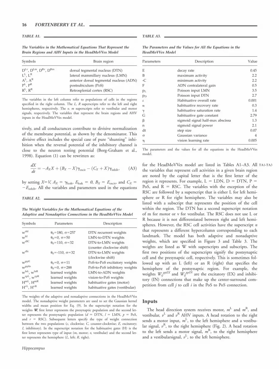
TABLE A1.

The Variables in the Mathematical Equations That Represent the

Brain Regions and AHV Inputs in the HeadMoVVes Model

Symbols Brain region

DLv, DLm, DRv, DRm dorsal tegmental nucleus (DTN)

LL, LR lateral mammillary nucleus (LMN)

AL, AR anterior dorsal tegmental nucleus (ADN)

PL, PR postsubiculum (PoS)

RL, RR Retrosplenial cortex (RSC)

The variables in the left column refer to populations of cells in the regionsspecified in the right column. The L, R superscripts refer to the left and righthemispheres, respectively. The v, m superscripts refer to vestibular and motorsignals, respectively. The variables that represent the brain regions and AHVinputs in the HeadMoVVes model.

TABLE A2.

The Weight Variables for the Mathematical Equations of the

Adaptive and Nonadaptive Connections in the HeadMoVVes Model

Symbols Parameters Description

wdd u05180, r5257 DTN recurrent weights

wld u050, r550 LMN-to-DTN weights

wdlC u05110, r532 DTN-to-LMN weights

(counter clockwise shift)

wdlc u05-110, r532 DTN-to-LMN weights

(clockwise shift)

wppE u050, r511 PoS-to-PoS excitatory weights

wppIn u050, r5288 PoS-to-PoS inhibitory weights

wlaL, wlaR learned weights LMN-to-ADN weights

wrpL, wrpR learned weights vision-to-PoS weights

HmL, HmR learned weights habituative gates (motor)

HvL, HvR learned weights habituative gates (vestibular)

The weights of the adaptive and nonadaptive connections in the HeadMoVVesmodel. The nonadaptive weight parameters are used to set the Gaussian kernelwidths and mean position for Eq. (9). In the superscript notation for theweights W, first letter represents the presynaptic population and the second let-ter represents the postsynaptic population (d 5 DTN, l 5 LMN, p 5 PoS,and r 5 RSC). Subsequent letters specify the type of weight connectionbetween the two populations (c, clockwise; C, counter-clockwise; E, excitatory;I, inhibitory). In the superscript notation for the habituative gates (H) is thefirst letter represents type of input (m, motor; v, vestibular) and the second let-ter represents the hemisphere (L, left; R, right).

TABLE A3.

The Parameters and the Values for All the Equations in the

HeadMoVVes Model

Parameters Description Value

E decay rate 0.45

B maximum activity 2.2

-C minimum activity 2.2

F ADN contralateral gain 0.5

pL Poisson input LMN 3.5

pD Poisson input DTN 2.7

e Habituative overall rate 0.001

a habituative recovery rate 0.3

g habituative saturation rate 1.4

G habituative gate constant 2.79

b sigmoid signal half-max abscissa 1.3

n sigmoid signal power 2.1

dt step size 0.07

r Gaussian variance 4

h vision learning rate 0.005

The parameters and the values for all the equations in the HeadMoVVesmodel.

TA1-TA3


Hippocampus

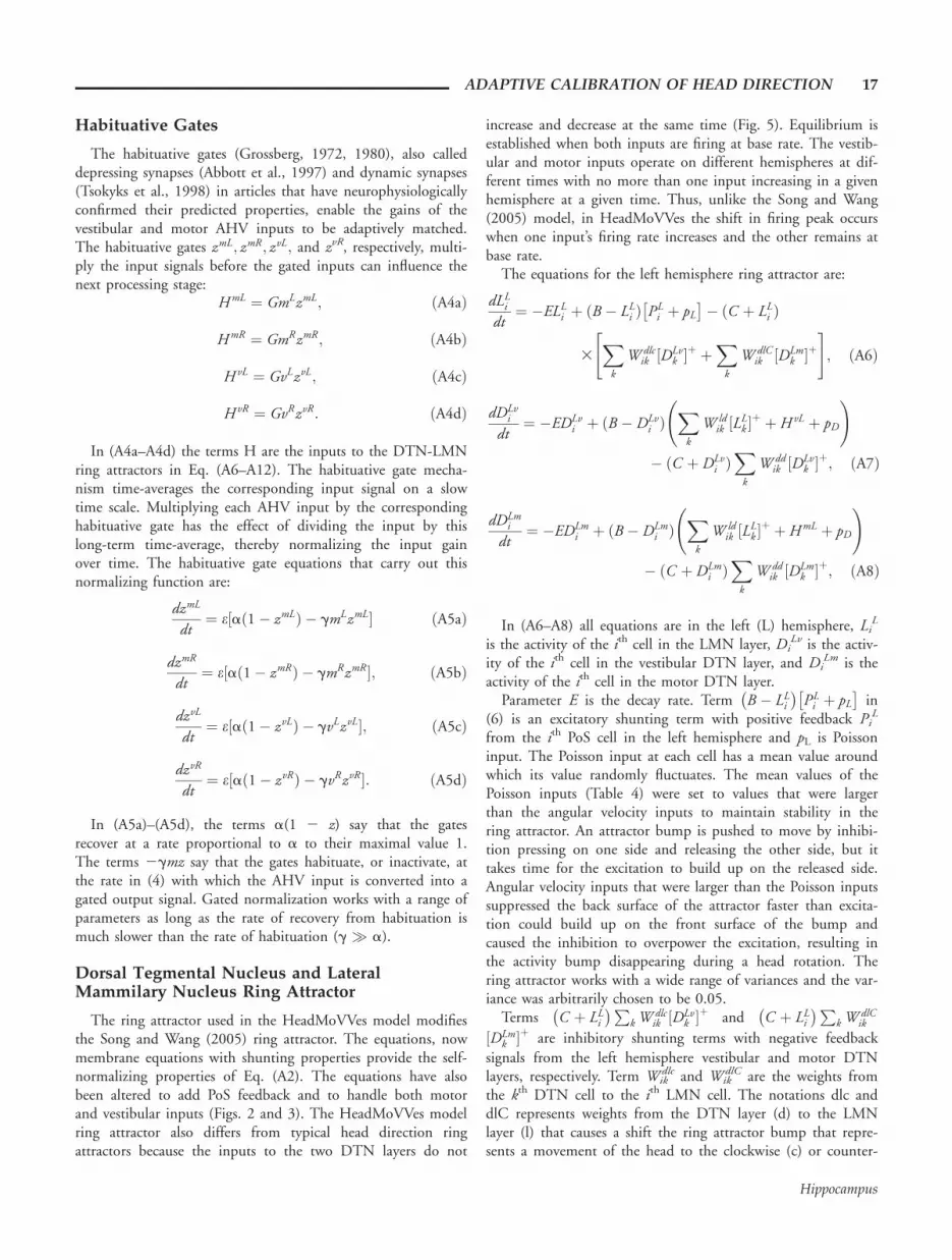
Habituative Gates

The habituative gates (Grossberg, 1972, 1980), also calleddepressing synapses (Abbott et al., 1997) and dynamic synapses(Tsokyks et al., 1998) in articles that have neurophysiologicallyconfirmed their predicted properties, enable the gains of thevestibular and motor AHV inputs to be adaptively matched.The habituative gates zmL; zmR; zvL; and zvR, respectively, multi-ply the input signals before the gated inputs can influence thenext processing stage:

HmL ¼ GmLzmL; ðA4aÞ

HmR ¼ GmRzmR ; ðA4bÞ

HvL ¼ GvLzvL; ðA4cÞ

HvR ¼ GvRzvR: ðA4dÞ

In (A4a–A4d) the terms H are the inputs to the DTN-LMNring attractors in Eq. (A6–A12). The habituative gate mecha-nism time-averages the corresponding input signal on a slowtime scale. Multiplying each AHV input by the correspondinghabituative gate has the effect of dividing the input by thislong-term time-average, thereby normalizing the input gainover time. The habituative gate equations that carry out thisnormalizing function are:

dzmL

dt¼ e½að1� zmLÞ � gmLzmL� ðA5aÞ

dzmR

dt¼ e½að1� zmRÞ � gmRzmR�; ðA5bÞ

dzvL

dt¼ e½að1� zvLÞ � gvLzvL�; ðA5cÞ

dzvR

dt¼ e½að1� zvRÞ � gvRzvR�: ðA5dÞ

In (A5a)–(A5d), the terms a(1 2 z) say that the gatesrecover at a rate proportional to a to their maximal value 1.The terms 2gmz say that the gates habituate, or inactivate, atthe rate in (4) with which the AHV input is converted into agated output signal. Gated normalization works with a range ofparameters as long as the rate of recovery from habituation ismuch slower than the rate of habituation (g � a).

Dorsal Tegmental Nucleus and LateralMammilary Nucleus Ring Attractor

The ring attractor used in the HeadMoVVes model modifiesthe Song and Wang (2005) ring attractor. The equations, nowmembrane equations with shunting properties provide the self-normalizing properties of Eq. (A2). The equations have alsobeen altered to add PoS feedback and to handle both motorand vestibular inputs (Figs. 2 and 3). The HeadMoVVes modelring attractor also differs from typical head direction ringattractors because the inputs to the two DTN layers do not

increase and decrease at the same time (Fig. 5). Equilibrium isestablished when both inputs are firing at base rate. The vestib-ular and motor inputs operate on different hemispheres at dif-ferent times with no more than one input increasing in a givenhemisphere at a given time. Thus, unlike the Song and Wang(2005) model, in HeadMoVVes the shift in firing peak occurswhen one input’s firing rate increases and the other remains atbase rate.

The equations for the left hemisphere ring attractor are:

dLLidt

¼ �ELLi þ ðB � LLi Þ PLi þ pL

� �� ðC þ LLi Þ

3Xk

W dlcik ½DLv

k �þ þXk

W dlCik ½DLm

k �þ" #

; ðA6Þ

dDLvi

dt¼ �EDLv

i þ ðB � DLvi Þ

Xk

W ldik ½LLk �

þ þHvL þ pD

!

� ðC þ DLvi ÞXk

W ddik ½DLv

k �þ; ðA7Þ

dDLmi

dt¼ �EDLm

i þ ðB � DLmi Þ

Xk

W ldik ½LLk �

þ þHmL þ pD

!

� ðC þ DLmi ÞXk

W ddik ½DLm

k �þ; ðA8Þ

In (A6–A8) all equations are in the left (L) hemisphere, LiL

is the activity of the ith cell in the LMN layer, DiLv is the activ-

ity of the ith cell in the vestibular DTN layer, and DiLm is the

activity of the ith cell in the motor DTN layer.Parameter E is the decay rate. Term B � LLi

� �PLi þ pL

� �in

(6) is an excitatory shunting term with positive feedback PiL

from the ith PoS cell in the left hemisphere and pL is Poissoninput. The Poisson input at each cell has a mean value aroundwhich its value randomly fluctuates. The mean values of thePoisson inputs (Table 4) were set to values that were largerthan the angular velocity inputs to maintain stability in thering attractor. An attractor bump is pushed to move by inhibi-tion pressing on one side and releasing the other side, but ittakes time for the excitation to build up on the released side.Angular velocity inputs that were larger than the Poisson inputssuppressed the back surface of the attractor faster than excita-tion could build up on the front surface of the bump andcaused the inhibition to overpower the excitation, resulting inthe activity bump disappearing during a head rotation. Thering attractor works with a wide range of variances and the var-iance was arbitrarily chosen to be 0.05.

Terms C þ LLi� �P

k Wdlcik ½DLv

k �þ and C þ LLi� �P

k WdlCik

½DLmk �þ are inhibitory shunting terms with negative feedback

signals from the left hemisphere vestibular and motor DTNlayers, respectively. Term Wik

dlc and WikdlC are the weights from

the kth DTN cell to the ith LMN cell. The notations dlc anddlC represents weights from the DTN layer (d) to the LMNlayer (l) that causes a shift the ring attractor bump that repre-sents a movement of the head to the clockwise (c) or counter-


Hippocampus

clockwise (C) direction, respectively. Function DLvk

� �þis the

output signal from the kth DTN cell in the left (L) hemisphere

that receives vestibular (v) input. Function DLmk

� �þis the out-

put signal from the kth DTN cell in the left (L) hemisphere

that receives motor (m) input. Notation ½n�þ ¼ maxðn; 0Þmeans that the output signal is half-wave rectified with a zerooutput threshold.

In Eqs. (A7) and (A8), the term ½LLk �þ is the kth cell in

LMN layer in the Left (L) hemisphere, HvL is the habituativegated vestibular angular velocity input to the left hemisphere,and HmL is the habituative gated motor angular velocity inputto the left hemisphere. The parameter pD is tonic input to theDTN layers that fluctuates randomly according to Poisson dis-tribution (Table 4).

The kernels for the nonadaptive weights (Wld, WdlC, Wdlc,Wdd) are specified by the following equation:

Wik ¼ ecosðuk�ui�u0Þðrp=180�Þ2

� �; ðA9Þ

in (A9), uk is the head-centric position in degrees that is repre-sented by the presynaptic cell, ui is the head-centric position indegrees that is represented by the post-synaptic cell, and u0 is thedifference in degrees between the pre- and postsynaptic cells. Allkernels with the exception of the asymmetric weights from DTNto LMN have u0 5 0. The parameters are listed in Table 3.

The ring attractor in the right hemisphere is the same asthat in the left hemisphere except that the motor and vestibularDTN connections to the LMN are switched. To generate thedifferent shift directions, the weights WILE and WIRE areswitched. The equations for the right hemisphere are thus:

dLRidt

¼ �ELRi þ ðB � LRi Þ PRi þ pL

� �� ðC þ LRi Þ

3XK

W dlcik ½DRm

k �þ þXk

W dlCik ½DRv

k �þ" #

; ðA10Þ

dDRvi

dt¼ �EDRv

i þ ðB � DRvi ÞXk

W ldik ½LRk �

þ � ðC þ DRvi Þ

3Xk

W ddik ½DRv

k �þ þHvR þ pD; ðA11Þ

dDRmi

dt¼ �EDRm

i þ ðB �DRmi ÞXk

W ldik ½LRk �

þ � ðC þ DRmi Þ

3Xk

W ddik ½DRm

k �þ þHmR þ pD; ðA12Þ

Anterior Dorsal Thalamic Nuclei

The ADN is the brain region that combines the vestibularand motor signals (Fig. 3). The equations for the ADN leftand right hemispheres are:

dALi

dt¼ �EAL

i þ ðB � ALi Þ f ðLLj Þ þ Ff ðLRi Þh i

ðA13Þ

and

dARi

dt¼ �EAR

i þ ðB � ARi Þ f ðLRj Þ þ Ff ðLLi Þh i

; ðA14Þ

where the output signal function from the LMH to the ADNis a sigmoid signal:

f ðxÞ ¼ xn

bn þ xnðA15Þ

that narrows the width of the tuning curve. In (A13) and(A14), Ai

L and AiR are the activities of the ith ADN cells in the

left (L) and right (R) hemispheres. Parameter E is the decayrate. The term is the excitatory shunting term and signals

f LLj

� �and f LRj

� �is the LMN inputs from the left and right

hemispheres. The term F � 1 is a gain factor for the contralat-eral LMN connection which ensures that the contralateralinput is no stronger than the ipsilateral input. As F is chosencloser to 1, the activity in the two ADN layers will merge tothe same position. As F is chosen closer to 0, the activity in thetwo ADN layers will diverge to a gap that matches the differ-ence in LMN layers.

Postsubiculum

The PoS is a winner-take-all competition that chooses frommotor and vestibular inputs from the ipsilateral ADN and vis-ual inputs from the RSC. The competition is accomplished byrecurrent on-center off-surround interactions with the contralat-eral PoS. The excitatory connections use narrow and strongkernel, and the inhibitory connections (through inhibitory neu-rons; Fig. 6) use a diffused and weak kernel. The equations forthe PoS (without visual RSC input) in the left and right hemi-spheres are:

dPLi

dt¼ �EPL

i þ ðB � PLi Þ�ALi þ

Xj

WppEij PR

j

�� ðC þ PL

i Þ

3Xi

WppIij PR

j ; ðA16Þ

dPRi

dt¼ �EPR

i þ ðB � PRi Þ�ARi þ

Xj

WppEij PL

j

�� ðC þ PR

i Þ

3Xi

WppIij PL

j ; ðA17Þ

In (A16 and A17), PiL is the activity in the ith PoS cell and

L and R signify the hemisphere. The term E is the decay rate.

The term ðB � PLi ÞðAL

i þP

j WppEij PR

j Þ is the excitatory shunt,

AL is the excitatory input from the ipsilateral ADN, WijppE is

the excitatory weight connection from the ith ADN cell to theith PoS cell, and PR is the activity from jth cell in the contralat-

eral PoS. The term ðC þ PLi ÞP

i WppIij PR

j is the inhibitory

shunt and WijppI is the inhibitory weight. The kernels for the

nonadaptive weights (W ppE ;W ppI ) are specified by Eq. (9).


Hippocampus

Retrosplenial Cortex

The object-in-place cells of the RSC give equal salience toall objects and do not encode object size and distance. Thewidth and strength of the object is represented by a Gaussiancurve that is centered at the position at which the animat viewsthe object in head-centric coordinates. Thus:

Rni ¼ e �ðui�u0Þ2

2r2

� �; ðA18Þ

where Rin is the RSC cell in ith cell position of the nth object.

The term ui 2 u0 is the number of degrees of the ith cell posi-tion from the center of the object. Parameter r2 defines thevariance of the Gaussian.

The RSC weights are updated by the current PoS HD esti-mate. The RSC assumes that the PoS HD estimate is accu-rate at every moment in time. The learning rule is presynap-tically gated, such that the weights will only update if theobject representing the RSC layer is visible. The weightsmove towards the product or correlation of pre- and postsy-naptic activities and anchor the visual landmark to the cur-rent PoS HD estimate, such that if the PoS cell activity islarge the weights will increase but if the PoS cell activity isweak the weights will decrease. The RSC weight update ruleis defined by:

dWrpnLij

dt¼ h PL

j Rni �W

rpnLij

h iRni ; ðA19Þ

in (A19), WrpnLij is the weight from the ith RSC cell in the nth

RSC object layer projecting to the jth PoS cell in the Left (L)hemisphere. The term h is the learning rate, Pj

L is the PoS cellat the jth position in the left hemisphere, and Ri

n is the ith

RSC cell in the nth object layer.The PoS layer with vision is the same equation as the PoS layer

without vision in equations (A16 and A17), with the exception ofthe last excitatory shunting term. The PoS receives input from ev-ery vision cell in the RSC but only a few cells are active and anygiven time. The left hemisphere PoS equation with vision:

dPLi

dt¼ �EPL

i þ ðB � PLi ÞAL

i þ ðB � PLi Þ

3Xj

wppEij PR

j � ðC þ PLi ÞXi

WppIij PR

j þ ðB � PLi Þ

3Xn

Xj

WrpnLij Rn

j : ðA20Þ

The first portion of the equation is explained in equations(16 and 17). The last term is an excitatory shunt, where W

rpnLij

is the weight from the ith RSC cell in the nth RSC object layerprojecting to the jth PoS cell in the Left (L) hemisphere andRi

n is the ith RSC cell in the nth object layer.


Hippocampus

learned integration of visual, vestibular, and motor cues in multiple brain regions computes head...

Documents