lattice gas models in contact with stochastic reservoirs: local equilibrium and relaxation to the...

commun. Math. Phys. 140,119131 (1991) Communications in

MathematicalPhysics

© Springer-Verlag 1991

Lattice Gas Models in Contact with StochasticReservoirs: Local Equilibrium and Relaxationto the Steady State*

Gregory Eyink1'2, Joel L. Lebowitz1 and Herbert Spohn2

1 Departments of Mathematics and Physics, Rutgers University, New Brunswick, NJ 08903, USA2 Theoretische Physik, Universitat Miinchen, W-8000 Munchen, Federal Republic of Germany

Received October 1, 1990

Abstract. Extending the results of a previous work, we consider a class of discretelattice gas models in a finite interval whose bulk dynamics consists of stochasticexchanges which conserve the particle number, and with stochastic dynamics atthe boundaries chosen to model infinite particle reservoirs at fixed chemicalpotentials. We establish here the local equilibrium structure of the stationarymeasures for these models. Further, we prove as a law of large numbers that thetime-dependent empirical density field converges to a deterministic limit processwhich is the solution of the initial-boundary value problem for a nonlinear diffusionequation.

1. Introduction

We continue our study of the hydrodynamics of stochastic lattice gas models ina finite interval, with stochastic dynamics at the boundaries chosen to model theinteraction with infinite particles reservoirs at fixed chemical potentials, which webegan in our earlier paper [ELS] (hereafter referred to as I). We remind thereader that the model under consideration is a continuous-time Markov processon the finite state space Ω = {0,1}Λ, where A = [ - M, M] nZ is a lattice of (2M + 1)sites. The components ηx,xeλ of the state vector ηeΩ denote the occupationnumbers of the sites x (1 = occupied, 0 = vacant). We refer the reader to I for anexplicit definition of the stochastic dynamics, only pointing out here thatfinite-range, translation-invariant, non-degenerate rates are required, satisfyinglocal detailed balance conditions and the technical "gradient" condition.

* Supported in part by NSF Grants DMR89-18903 and INT85-21407. G.E. and H.S. alsosupported by the Deutsche Forschungsgemeinschaft

120 G. Eyink, J. L. Lebowitz and H. Spohn

In I we studied the unique stationary measure of the lattice gas for large Mon a hydrodynamic scale. In particular, we proved that the empirical density fieldobeys a law of large numbers with respect to the stationary measures με

ss (ε = M ~ 1 ) ,converging weakly as ε -• 0 to a deterministic limit, which is given as the solutionof a stationary transport equation. More generally, we showed that every extensivefield defined by a bounded, local quantity obeys such a law of large numbers,converging to a deterministic limit which is an appropriate function of the localdensity. The proofs of these assertions were based on an entropy productionargument of Guo, Papanicolaou and Varadhan [GPV], adapted to the situationwith stochastic boundary dynamics.

We improve the analysis of the stationary measure, by showing that thestrongest result obtainable by the GPV type of argument is a pointwise versionof the local equilibrium property (LEP) for the stationary measure με

ss (a strongerresult than the L2 version we claimed in I). By this we mean the assertion that forany bounded, local function g(η\

for every qe(— 1,1), where p is the solution of the stationary transport equationwith boundary conditions p(± 1) = ρ(λ + ) = p + and < >p is the expectation withrespect to the infinite-volume Gibbs measure (for Hamiltonian H) at density p.Therefore, the stationary measures have the property that the expectations of anylocal function at a fixed position q on the macroscopic scale converge to thecorresponding equilibrium expectations with the local value of the density p(q).The original argument of GPV does not yield this result, since their proof dependedupon establishing small entropy production for space-time averaged measures.Our argument relies upon having sufficiently good local bounds on the entropyproduction (i.e. bounds on the entropy production of marginal distributions inlocal blocks, going to zero as ε->0) which follow automatically in theone-dimensional case from the global entropy bound and monotonicity of theentropy production. A further element of our proof is a local form of the two-blockestimate of I which permits one to "tie together" neighboring blocks. Localequilibrium was obtained previously for the special case of symmetric simpleexclusion dynamics by a duality argument [GKMP].

Next, we turn our attention to the time-dependent behavior of our stochasticdynamical system. In particular, we study the relaxation of initial local equilibriumdistributions to the final steady state on the hydrodynamic scale. The goal hereis to verify that the time-dependent empirical density field is given, in thehydrodynamic limit, by the solution of the initial-boundary value problem for thenonlinear diffusion equation: that is, by p(q, τ) which solves

dτp(q,τ) = dqlD(p(q9τ))dqp(q,τ)l (<?,τ)e[-1,1] x [0, Γ ] , (1.9)

P(q,0) = p0(q), qe[-l,ll (1.10)

p(±l9τ) = p±9 τe[0,T] (1.11)

for specified initial data po(q) and boundary values p±= p(λ±). As in the staticcase, D(p) is the bulk diffusion coefficient for the dynamics, given by a G r e e n - K u b oformula (see [ S p , D I P P ] ) .

Lattice Gas Models in Contact with Stochastic Reservoirs 121

The proof of the local equilibrium property for the stationary measures is thecontent of Sect. 2. The hydrodynamic relaxation to the steady state is discussedin Sect. 3. We freely borrow notations and definitions from I (e.g. we refer thereader to Sect. 2 of I for the definition of entropy production for our models). Theresults of Sect. 2 of I, in particular the fundamental Proposition 1 and itsconsequence Lemma 4, are the core of our present arguments, as they were of thestatic law of large numbers in I. We also continue the numbering of propositionsof I, for the ease of reference of the reader.

2. Local Equilibrium Property of the Stationary Measures

Our goal is to prove the local equilibrium property of the stationary measure inthe following precise form:

Theorem 3. For any bounded, local function g(η\

q) (2.1)ε->0

for all qe(— 1,1) (where <•> denotes expectation with respect to the infinite-volumeGibbs measure at density p). Further, for any g supported in Έτ, if </>J denotesexpectation with respect to the Gibbs measure on the semi-infinite domain ΊL + withfree boundary conditions and asymptotic density p,

Proof. We consider first the case (2.1), where we have the inequality

\s(A(g,lε'ι(q-ϊ),e,-ι(q + / ) ] ) ) - - J dq'g(β(q'))

q + l

2 l [ dqfg(p(q'))-g(p(q)), (2.3)

and we employ the notation from I that

1

Έ<J^ Σ gM {2A)

for any interval B, and

g(p) = <g>P (2.5)

Clearly, for each qe(— 1,1), the last term on the right-hand side of (2.3) goes tozero as /-*0. On the other hand, the middle term goes to zero as ε->0 by theweak convergence of the extensive functions, established in I, and the boundednessof g(η) and, consequently, of the averages A(g,B).

Finally, we prove for the first term that, for each qe(— 1,1),

Jim Jim \με

ss(glε-ιq}) - με

ss(A(β> ^'(i ~ lU'Hq + 0]))l = 0,


which yields the first statement of the theorem. To obtain this result we shallmodify the strategy of the proof for Proposition 1. We observe the inequality

% , ] ) ) l + ^ r Σ με

ss(\A(g,B0)-A(g,Bj)\), (2.6)ZL, j= -L

L

where [ε" ι{q - /), ε" ι(q + /)] = [j Bj9 L = {l/εk}, and the 2L B/s are blocks ofJ=-L

k sites each, disjoint, with [ε~ ιq\ at the center of Bo. We introduce also the blocksBj of k — 2R sites, obtained by removing the R border sites at the ends of eachBj (R the range of the interaction). We see that it suffices to prove

i) lim \με

ss(gίε-lq]) - μl(A(g,Bo))\ = 0, (2.7)

ii) lim Kmlϊmsvφμl(\A{g9Bo)-A{g9Bj)\) = 0. (2.8)fc->oo f-»0 ε->0 j

For i), we will use the fact that the limiting canonical Gibbs measures as ε -• 0are translation-invariant (in the infinite-volume limit, i.e. as fc-» + oo). To makethe argument precise, introduce a block of r spins B'o => Bo, r> fc, and let με

q r bethe marginal of με

ss on B'o, considered as a measure on configurations in a fixed

[ r r\— , - .By the main entropy production bound and monotonicity,

2 2 J Z

σB,Lμlr-]^cε. (2.9)

Hence, any weak limit point μ*r of με

qr as ε -• 0 must be a convex combination of

Γ r r~\the canonical Gibbs measures ^ c on — , - . In particular,

L 2 2JJ o))l = Πm |μjfΓto0) - μ ^ t o , Bo)) I

^ sup |vNto0)-vN(>lto,B0))|, (2.10)iV = 0,...,r

where vN is the canonical Gibbs measure on B'o with iV particles (actually, weshould also specify the fixed occupancies ηB in the boundary regions oϊBr

0 of widthR, as vNrjB - for simplicity, we have neglected this.) Because, for each r, the sup isrealized for some Nr and since there is the bound 0 ^ Nr/r ^ 1, a subsequence (ry)may be chosen so that r7 | + oo and

^ ( 2 . 1 1 )

It follows that for each fc,

δ iVr to0) - vNr (A(g,Bo))\j J

= 0, (2.12)

the latter by the translation-invariance of the Gibbs measure. This gives i).


For ii), we employ a modified version of the argument for the two-block estimatein Theorem 1. For each ε, / the supremum in (2.8) is achieved for some j ε l . Foreach ε, / we define με\ to be the joint marginal of με

ss in the two blocks Bo andΓ (k \ k Ί

B. , considered as a measure on the fixed set {0,1} x —I — R I , — R\Γ ίk \ k 1 L \2 / 2 J z

consisting of two copies of —I — R L — R , denoted Bo and Bt. Define,L \2 / 2 J z

then, as in Theorem 1, the Dirichlet form

£oi(/)—-L Σ Σ <c(x,y;η)U(ηxy)-f(riΏ2>P (2.13)

for / the density of a measure on BQΌB^ Furthermore, introduce

(2-14)

As a consequence of the main entropy estimate and the Lemma 2 of I, we have that

^ o u ^ C / ^ 3 ^const.ε + const./. (2.15)

Therefore, any limit point f*k of p£k as ε->0 and then /->() must haveσ B o U β i [ / * k ] = 0. Note, however, that the functional σBoKjBi has the same essentialproperties for BouBί as σBo has for Bo alone: it is a positive, convex function,which is strictly convex on the set of /'s which have fixed occupancies on theboundary regions of each block and fixed total (combined) number of particles inthe two boxes. Hence, there is a unique value / m i n in that domain where theminimum value σ β o U β i [ / m i n ] = 0 is attained and it is easy to verify that / m i n isthe finite version of a canonical Gibbs measure on BouBι with specifiedoccupancies outside. Therefore, the limit points /* f c are in the set of convexcombinations of such extremal elements. Hence,

lΐm lim sup με

ss(\Λ(g, Bo) - A{g, Bj)\)ί->0 ε-"0 j

ί sup vN(\A(g,B0)-A(g,B1)\). (2.16)N = 0,...,2fc-4K

We may argue as before that for each fe, the supremum is actually achieved forsome Nfce{0,...,2k — 4R} and then, since,

0 ^ — ^ 1 , (2.17)2k

along any subsequence for which vNk(\A(g,B0) — A(g,Bι)\) converges, a furthersubsequence kj may be chosen so that

Ί1 .^ r - . - , - ] • (2-18)

Then, by the L1 law of large numbers for the canonical ensemble,

ϊimvNk(\A(g,B0)-A(g,B1)\)^:hmvNk(\A{g,B0)-g(p)\)j-HX) J J-+CO J

+ foivNk(\A(g,B1)-g(p)\)j-*O0 i

= 0, (2.19)


so that the subsequence of vNk(\Λ(g,Bo) — A(g,fiJI) necessarily converges to zero.Thus,

lϊm ϊΐm ϊϊm sup με

ss(\A(g,Bo) - A{g9B1)\) = 0, (2.20)k-+0 ί->0 ε->0 j

which gives ii).The second part of the theorem, embodied in (2.2), is somewhat easier to prove.

Consider the right endpoint. We may write

for every r for which suppg £ [— r,0], where f\ r is the density with respect tothe Gibbs measure vp of the marginal of με

ss in the interval [M — r — R,M~\π,considered as a measure on configurations in a fixed interval [— r — Λ,0] z . In theproof of Proposition 1 in I, it was shown that, for each r, the limit / * r of f\ r asε->0 exists and equals the density of the Gibbs measure at density p+ on theinterval [— r — Λ,0] z , with free boundary conditions at the right endpoint andspecified distribution in the left boundary interval [— r — R, — f]π. Therefore,

μi(0M) < / * r 0 > p . (2.22)£-•0

Since r is arbitrary, we may take subsequently r-+ + oo. Since the system ofconditional distributions of μ* r converge in this limit to a consistent set ofconditional distributions on the subsets of the semi-infinite interval [— oo,0] z,satisfying the lattice DLR equations with chemical potential λ(p + ) and freeboundary conditions at the right end, and since the Gibbs measure is unique inone dimension (e.g. see [G]), it follows that

\imμε

ss(gM) = (g};+. (2.23)

This completes the proof of Theorem 3. •

We remark that the local equilibrium property is a stronger result than theweak convergence of the extensive fields. A relatively simple argument using theChebyshev inequality gives the convergence in probability to a deterministic limit,which, with tightness, gives the weak convergence (see [DIPP], Proposition 4.1).However, local equilibrium does not apparently follow from the weak convergenceresult alone (but, rather, as above, from its proof).

3. Relaxation to the Steady State

For the model introduced in I, we will now consider the stochastic process^ J c ε - 2 r , 0 ^ τ ^ T , x = — ε ~ 1 , . . . , ε " 1 , ( ε ~ 1 = M ) with the initial measures με requiredto satisfy for each δ > 0 and φe@([- 1,1]),

1

limμf

X°0(φ)- I dqφ(q)po(q)- 1

>δ = 0 (3.1)

for some fixed pQeJiu where, as in I, Jίγ = LJ°([— 1,1]) is the set of non-negativemeasurable functions on [—1,1] essentially bounded by one. In this section, Pε

denotes the path measure for the process and Eε the corresponding expectation.


We regard τi—>pε, with pε

τ(q) = η^ε- i^ ε-2 τ, as an element of D([0, Γ], Jίx\ the spaceof right continuous trajectories, with left limits equipped with the Skohorodtopology. The path measure P ε induces a path measure on D([0, T~\,Jίx)\ withoutrisk of confusion, this measure is again denote by Pε, expectations by Eε.

We define ρeL™([ — 1,1] x [0, T]) to be a weak solution of the initial-boundaryvalue problem (4.1-3) if,for every </>eC2([- 1,1]) with (/>(+l) = 0anda.e.τe[0, T],

1 1

J dqφ(q)p(q,τ)- J dqφ(q)po(q)- 1 - 1

= ]dσ\ J dqφ'\q)h{p{q,σ))-φ\ + l)h(p + )-^ φf(-l)h(p~)\ (3.2)o L-i J

For every poeJί1 and p + E [ 0 , 1] there exist solutions of (3.2), which are furthermoreunique under an additional regularity assumption, such as peL2([0, Γ] ,Hj + p)with HQ the Sobolev space of functions with L2 derivatives which vanish at q = ±1(see below). Given poeJ(l9 we define the measure P = δp on Z)([0, T\Jix\ wherep is the unique weak solution corresponding to initial data p 0 .

The main result we claim in this section is:

Theorem 4. P is the weak limit of Pε as ε->0.

As for the static result in I, the proof of Theorem 4 requires an estimate on entropyproduction which is provided by

Proposition 4. Ifμε = fεvε

p is an arbitrary measure on {0, \}Λand με is its time-averageover the interval [0, ε~ 2τ], with density given by

4rIε τ o

(L* denotes the adjoint ofL with respect to vp), then, for σ ε [/ ε ] the entropy productiondefined in (I; 2.1),

W Λ (3.4)

for some c>0; in particular, μεeS(ε) = {/ |σ ε[/] ^cε, f ^ 0 , < / > ε = 1}.

This proposition allows again the application of the fundamental Proposition 1and its consequence Lemma 4 of I to the present situation. The proof of Theorem 4itself requires the verification of two key statements:

(1) (Pε |ε > 0) is a tight family.(2) If P* is any weak limit of the family as ε->0, then P* is supported byC([0, T]9J(ι)nL2(l09Γ\9Hl + β) and for every φeC\- 1,1] with 0 ( ± 1 ) = O andevery τe[0, Γ],

dqφ(q)lp(q,τ)-po(q)~]- 1

= }dσ\ Jo L-i

-a.s . . (3.5)


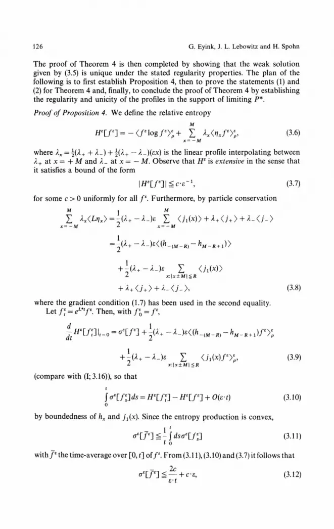
The proof of Theorem 4 is then completed by showing that the weak solutiongiven by (3.5) is unique under the stated regularity properties. The plan of thefollowing is to first establish Proposition 4, then to prove the statements (1) and(2) for Theorem 4 and, finally, to conclude the proof of Theorem 4 by establishingthe regularity and unicity of the profiles in the support of limiting P*.

Proof of Proposition 4. We define the relative entropy

^ + Σ ^<ff x /% (3.6)

where λx = j(λ++λ-) + j(λ+— /l_)(εx) is the linear profile interpolating betweenλ+ at x = + M and λ- at x = — M. Observe that Hε is extensive in the sense thatit satisfies a bound of the form

\Win\^cε-\ (3.7)

for some c>0 uniformly for all fε. Furthermore, by particle conservation

x=-M 2- x=-M

= - μ + -

+ \(λ+-λ_)ε X2 x:\x±M\^R

(3.8)

where the gradient condition (1.7) has been used in the second equality.Let f\ = eL*'fe. Then, with fε

0 = fε,

+ l-(λ+-λ_)ε Σ <ji(x)/e>', (3.9)^ x:\x±M\^R

(compare with (I; 3.16)), so that

+ O(β-t) (3.10)0

by boundedness of hx and j^x). Since the entropy production is convex,

\%ps\ (3.11)t o

with/ε the time-average over [0, t] of/ε. From (3.11), (3.10) and (3.7) it follows that

~ + c ε, (3.12)ε ί


and, in particular,

( \ (3.13)

with t = ε~2τ. This is just the conclusion of Proposition 4. •

We now verify the key statements (1) and (2) for Theorem 4.

Ad (1): This can be accomplished by a standard machinery. We note that forφe@{\_- 1,1]) and ε sufficiently small (so that φ(εx) = 0 for |x ± M| g R)

ε~ 1

ε~2LXε(φ) = ε £ ε~2(φ(εx + ε) + φ(εx - ε) - 2φ(εx))hx(η)x=-ε~ι

= Xε(h;φ") + O(ε) (3.14)

and

ε ~ 2 ( L X \ φ f - 2X\φ)-LX*{φ)) = X (φ(εx) - φ(εx + ε ) ) 2 φ , x + l η)x=-ε~ι

= εXε(c;(φ')2) + O(ε2). (3.15)

Letε~ ι

Xε

t(Φ) = ε Σ Φ(εx)ηε^τ(x)- (3 1 6 )x= — ε~ x

The associated martingale, M\(φ\ is given by

X°τ(φ) - Xl(φ) = J dσε-2LX\φ)(ηt^σ) + M'τ(φ) (3.17)0

with the quadratic variation

E%M*τ(φ)2) = ε~2]dσE*(LX*σ(φ)2 -2X*σ{φ)LX*σ{φ)). (3.18)0

Let

fUτ(φ) = ε-2LX*(φ) (3.19)

and

f2yt(φ) = t-\LX*τ(φf - 2X](φ)LX'τ(φ)). (3.20)

Then, by (3.14) and (3.15), there exists a constant c, independent of ε and φ, such that

E'(γ\<t(φ)2)£c J ά ? < W (3.21)- 1

and

Eε(7lτ(φ)2) ^ M J dqφ\q)2Y. (3.22)

This implies tightness of the family (Pε |ε > 0) [M, DIPP].


Furthermore, any weak limit P* is supported on the set of continuoustrajectories C([0, T\J(^) because X\(φ) changes in a jump at most by H^'ILe2.

Ad (2): It is useful here to consider the fields Xε'k(φ) "cut-off" a finite microscopicdistance k from the boundaries:

φ(εx)ηx. (3.23)x=-ε~ι+k

If we consider φeC2([- 1,1]) with φ(± 1) = 0 but permit φ'{± 1) φ 0, then (3.14)must be replaced by

s-2LXε>k(φ) = ε ε~2(φ(εx + ε) + φ(εx - ε) - 2φ(εx))hx(η)

- sk)hM_k + 1 - φ{\ - εk + ε)hM_ J

Defining as above

y$*(φ) =

we find similarly the bound

= X%h;φ") + 0'(l)[(/c - l)fcM.k - khM_k+ J

M + J k _ 1 - ( f c - l ) Λ _ M + J + O

f (φ)2 - 2X<-k{φ) LXΐk(φ))9

<kΦ'(q)

(3.24)

(3.25)

(3-26)

It is important here to observe that this bound is independent of k. Since thequadratic variation of Mε*(φ) vanishes as ε ->0, we have, by Kolmogorov's Lemma,that

(3.27)

ε - 0lim EH sup I X?(φ) - Xf{φ) - j dσ[_Xf{h; φ")

- l)hM_k(ηε-2σ) -

uniformly in keΈ+. Hence, we also have, for each keZ+, that

lim£Ί sup0<τ<T

X?(φ)-X?(φ)-}dσ\x**(h;φ»)o L

1 k ! 1 w 1

'(1): Σ - Σ (0-1)K m = R Wl j = R

b'(-i)1- y ~mγ\jh

with

1 m'ί

Σ - Σ χtAΦ\m=Rmj=R

= 0 (3.28)

(3.29)


In terms of the average με of the initial measure με over the time-interval [0, ε 2 T],we have the bound

Eε[ sup

Λ k-l

— Σχ=-ε-ι+j

τί ε ^

- 0 ' -j fc-l , m - l ε - ' ( l - ί )

r Σ - Σ « ΣK t t l

Σ I,

m = R

1

kΣ -"Σm = R Wl j = R

fc-1 fc- 1 4 m ~( 2 4 m ~ ^

— Σ (Λ-^-t-SίP-M + r Σ - Σ(3.30)

using the summation by parts identity

j m—1 /j m-1

~ Σ Λm j=R

(3.31)

We see that this upper bound gives zero as first ε->0 and then fc-» oo, by usingProposition 1 and 4 and as well that

lim hmμ'fc 0

Λ+ ( M_Λ-Λ(/>±) (3.32)

which follows from Proposition 4 and the argument used to establish Proposition 1.We infer that

sup Xτ(φ)-X0(φ)-]dσ\ j dqφ"(q)h(p(q9σ))o L-i

= 0. (3.33)

This implies immediately the main statement (3.5) of (2).The regularity peL2([0, Γ], i/* 4- p) in the support of P* can be inferred from

1^0

dq(p'{q, τ))2)^ const. Γ,

hi

(3.34)

(3.35)


and/T /« - l + ί \ 2 \

lim£*(\dτ - f dqp(q,τ)-p\ =0, (3.36)

which are the consequences of Lemma 4 for a general μεeS(ε).Finally, we complete the proof of Theorem 2 by demonstrating the uniqueness

of weak solutions of (3.5) under the above regularity assumptions. Define R, forany p e L ? ( [ - 1 , 1 ] ) , by

R(x,y) = ]dqp(q). (3.37)X

1 1

We introduce the notation (F,G)= j dx j dyF{x,y)G(x9y).ΊhQn>iϊ peDdQ.T^Jί^- 1 - 1

Z1 ([ — 1,1]2), and R(τ) is associated to pτ{q) = p(q, τ) via (3.37), it follows that

l i p η(R(τ), Φ ) = f ^ f <iy jdqp(q,τ) \Φ(x,y)

-i - i Lx J

= J dqp(q,τ)φ(q)9 (3.38)- 1

with

= J dxfdyΦ(x,y)-fdx f dyΦ(x9y). (3.39)- 1 9 q - 1

Observe that φ e C 2 ( [ - 1,1]), </>(± l) = 0 and

0'te)= J dyΦ(q,y)- J dχφ(x^) . (3.40)- 1 - 1

If p is in the support of P*, it then follows that1

(R(τ),Φ)= I dqφ(q)Po(q)- 1

+ }dσ\ J dίr(ί)Λ(p(ί,σ)) + 0'(-l)Λ(p-)-^(l)Λ(p+)l (by (2))o L-i J

= ί d«0(ί)po(ί)-ί<iσ ί dqφ'(q)h(Py(q,σ), (3.41)- 1 0 - 1

by an integration by parts and the regularity assumption on p. Exploiting (3.40)gives finally

τ 1 1

(R(τ),Φ) = (R0,Φ) + fdσ f dx J dyΦ(x,y)[Λ(p)Ό;,σ)-*(/»)'(*.σ)], (3-42)0 - 1 - 1

i.e.

τ

, y; τ) = R0(x, y) + J A7[fc(py(y, σ) - h(p)'(x, σ)] (3.43)


in the L2-sense. Clearly, R(τ) is absolutely continuous in τ as a map into

L 2 ( [ - l , l ] 2 ) a n d

^R{x^τ) = h{p)\y,τ)-h{p)\x,τ\ a.e. τe[0,T], (3.44)dτ

with identity in the L2 sense.

Now consider for two weak solutions pγ and p2 of (3.5) the quantity

= Rί(τ)-R2(τ). (3.45)

From what we have shown above it follows that

^\\W(τ)\\2

2 = 2 j dx j dy(Rι(x,y;τ)-R2(x,y;τ))dτ -1 -1

• [(ft(Pi)'to τ) - h(P2)'(y, τ ) ) " (Λ(Pi)'(x,τ) - Λ(p2)'(x, τ))]

= - 8 f dMPi(y,τ)-p2(y,τ))(Λ(Pi(y,τ))-h(p2(y,τ)))^0. (3.46)- 1

the latter equality obtained by an integration by parts and the inequality by the

monotonicity of h. Since W(0) = 0, we conclude that for all τe[0, T]

W(τ) = 0 (3.47)

in an L2-sense; in particular, for all τe[0, T], a.e. (x9y)e[— 1,1]2,

)]=0. (3.48)

Therefore, p1= p2-This concludes the proof of Theorem 2. •

References

[DIPP] DeMasi, A., Ianiro, N., Pellegrinotti, A., Presutti, E.: A survey of the hydrodynamicalbehavior of many-particle systems. In: Nonequilibrium phenomena II. Lebowitz, J. L.,Montroll, E. W. (eds.), pp. 123-294. Amsterdam: North-Holland 1984

[ELS] Eyink, G., Lebowitz, J. L., Spohn, H.: Hydrodynamics of stationary nonequilibriumstates for some stochastic lattice gas models. Commun. Math. Phys. 132, 253-283(1990)

[GKMP] Galves, A., Kΐpnis, C, Marchioro, C, Presutti, E.: Nonequilibrium measures whichexhibit a temperature gradient: Study of a model. Commun. Math. Phys. 81, 127-148(1981)

[G] Georgii, H.-O.: Gibbs measures and phase transitions. Berlin, New York: Walter deGruyter 1988

[GPV] Guo, M. Z., Papanicolaou, G. C, Varadhan, S. R. S.: Nonlinear diffusion limit for asystem with nearest neighbor interactions. Commun. Math. Phys. 118, 31-59 (1988)

[M] Mitoma, I.: Tightness of probability measures on C([0,1],S") and D([0,1],S'). Ann.Probl. 11, 989-999 (1983)

[Sp] Spohn, H.: Large scale dynamics of interacting particles. To appear in Texts andMonographs in Physics. Berlin, Heidelberg, New York: Springer 1990

Communicated by A. Jaffe

lattice gas models in contact with stochastic reservoirs: local equilibrium and relaxation to the...

Documents