arX

iv:1

212.

1559

v2 [

astr

o-ph

.SR

] 1

0 D

ec 2

012

Accepted for publication on Advances in Astronomy

Latitudinal Dependence of Cosmic Rays Modulation

at 1 AU and Interplanetary-Magnetic-Field Polar

Correction

P Bobik1, G Boella2, MJ Boschini2,3, C Consolandi2,4, S Della

Torre2,5, M Gervasi2,4, D Grandi2, K Kudela1, S Pensotti2,4, PG

Rancoita2, D Rozza2,5, M Tacconi2,4

1 Institute of Experimental Physics, Kosice (Slovak Republic)2 INFN Milano-Bicocca, Milano (Italy)3 CILEA, Segrate (Milano, Italy)4 University of Milano-Bicocca, Milano (Italy)5 University of Insubria, Como (Italy)

E-mail: piergiorgio.rancoita@mib.infn.it

Abstract. The cosmic rays differential intensity inside the heliosphere, for energy below 30GeV/nuc, depends on solar activity and interplanetary magnetic field polarity. This variation,termed solar modulation, is described using a 2-D (radius and colatitude) Monte Carlo approachfor solving the Parker transport equation that includes diffusion, convection, magnetic driftand adiabatic energy loss. Since the whole transport is strongly related to the interplanetarymagnetic field (IMF) structure, a better understanding of his description is needed in orderto reproduce the cosmic rays intensity at the Earth, as well as outside the ecliptic plane. Inthis work an interplanetary magnetic field model including the standard description on eclipticregion and a polar correction is presented. This treatment of the IMF, implemented in theHelMod Monte Carlo code (version 2.0), was used to determine the effects on the differentialintensity of Proton at 1AU and allowed one to investigate how latitudinal gradients of protonintensities, observed in the inner heliosphere with the Ulysses spacecraft during 1995, can beaffected by the modification of the IMF in the polar regions.

1. Introduction

The Solar Modulation, due to the solar activity, affects the Local Interstellar Spectrum (LIS)of Galactic Cosmic Rays (GCR) typically at energies lower than 30 GeV/nucl. This process,described by means of the Parker equation (e.g., see [1, 2] and Chapter 4 of [3]), is originatedfrom the interaction of GCRs with the interplanetary magnetic field (IMF) and its irregularities.The IMF is the magnetic field that is carried outwards during the solar wind expansion. Theinterplanetary conditions vary as a function of the solar cycle which approximately lasts elevenyears. In a solar cycle, when the maximum activity occurs, the IMF reverse his polarity. Thus,similar solar polarity conditions are found almost every 22 years [4]. In the HelMod MonteCarlo code version 1.5 (e.g., see Ref. [2]), the “classical” description of IMF, as proposed byParker [5], was implemented together with the polar corrections of the solar magnetic fieldsuggested subsequently in [6, 7]. This IMF was used inside the HelMod [2] code to investigatethe solar modulation observed at Earth and to partially account for GCR latitudinal gradients,

– 2 –

i.e., those observed with the Ulysses spacecraft [8, 9]. In order to fully account for both thelatitudinal gradients and latitudinal position of the proton-intensity minimum observed duringthe Ulysses fast scan in 1995, the HelMod Code was updated to the version 2.0 to include anew treatment of the parallel and diffusion coefficients following that one described in Ref. [10].In the present formulation, the parallel component of the diffusion tensor depends only on theradial distance from the Sun, while it is independent of solar latitude.

2. The Interplanetary Magnetic Field

Nowadays, we know that there is a Solar Wind plasma (SW) that permeates the interplanetaryspace and constitutes the interplanetary medium. In IMF models the magnetic-field lines aresupposed to be embedded in the non-relativistic streaming particles of the SW, which carriesthe field with them into interplanetary space, producing the large scale structure of the IMF andthe heliosphere. The “classical” description of the IMF was proposed originally by Parker (e.g.,see [2, 5, 11, 12, 13, 14] and Chapter 4 of [3]). He assumed i) a constant solar rotation withangular velocity (ω), ii) a simple spherically symmetric emission of the SW and iii) a constant(or approaching an almost constant) SW speed (Vsw) at larger radial distances (r), e.g., forr > rb ≈ 10R⊙ (where R⊙ is the Solar radius), since beyond rb the wind speed varies slowlywith the distance. The “classical” IMF can be analytically expressed as [15]

BPar =A

r2(er − Γeϕ)[1 − 2H(θ − θ′)], (1)

where A is a coefficient that determines the IMF polarity and allows |BPar| to be equal to B⊕,i.e., the value of the IMF at Earth’s orbit as extracted from NASA/GSFC’s OMNI data setthrough OMNIWeb [16, 17]; er and eϕ are unit vector components in the radial and azimuthaldirections, respectively; θ is the colatitude (polar angle); θ′ is the polar angle determiningthe position of the Heliospheric Current Sheet (HCS)[18]; H is the Heaviside function: thus,[1− 2H(θ− θ′)] allows BPar to change sign in the two regions above and below the HCS [18] ofthe heliosphere; finally,

Γ = tanΨ =ω(r − rb) sin θ

Vsw

(2)

with Ψ the spiral angle. In the present model ω is assumed to be independent of the heliographiclatitude and equal to the sidereal rotation at the Sun’s equator. The magnitude of Parker fieldis thus:

BPar =A

r2

√

1 + Γ2. (3)

In 1989 [6], Jokipii and Kota have argued that the solar surface, where the feet of the fieldlines lie, is not a smooth surface, but a granular turbulent surface that keeps changing withtime, especially in the polar regions. This turbulence may cause the footpoints of the polar fieldlines to wander randomly, creating transverse components in the field, thus causing temporal

Period Years

I) A < 0 Ascending 1964.79–1968.87, 1986.70–1989.54, 2008.95–2009.95II) A < 0 Descending 1964.53–1964.79, 1979.95–1986.70, 2000.28–2008.95III) A > 0 Ascending 1976.20–1979.95, 1996.37–2000.28IV) A > 0 Descending 1968.87–1976.20, 1989.54–1996.37

Table 1. Definition of Ascending and Descending periods

– 3 –

0 10 20 30 40 50 60 70 80 90 100

0.1%

1%

10%

0° 10°20°30°40°50°60°70°80°90°0.0

5.0x10-61.0x10-51.5x10-52.0x10-52.5x10-53.0x10-53.5x10-54.0x10-54.5x10-55.0x10-5

b)

Rel

ativ

e di

ffere

nce

(BP

ol/B

Par-1

)

Solar Distance [AU]a)

20°; 1.2%

25°; 0.4%

30°; 0.2%

Latitude

Forbidden

m

Colatitude

Allowed

90° 80° 70° 60° 50° 40° 30° 20° 10° 0°

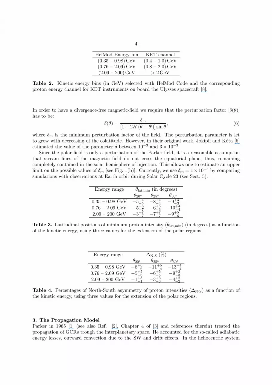
Figure 1. (a) Maximum percentage difference between BPol and BPar as a function of thesolar distance inside the colatitude regions 20◦ ≤ θ ≤ 160◦ (θ20◦), 25

◦ ≤ θ ≤ 155◦ (θ25◦) and30◦ ≤ θ ≤ 150◦ (θ30◦). (b) Maximum value allowed of δm as a function of colatitude: valuesin the “allowed” region guarantee that stream lines originated from the polar magnetic field donot cross the equatorial plane. Since Eq. (5) is symmetric with respect to the solar equatorialplane, values greater than 90◦ of colatitude lead to same results of those presented.

deviations from the smooth Parker geometry. The net effect of this is a highly irregular andcompressed field line. In other words, the magnitude of the mean magnetic field at the poles isgreater than in the case of the smooth magnetic field of a pure Parker spiral. Jokipii and Kota [6]have therefore suggested that the Parker spiral field may be generalized by the introduction of aperturbation parameter [δ(θ)] which amplifies the field strength at large radial distances. Withthis modification the magnitude of IMF, Eq.(3), becomes [6]:

BPol =A

r2

√

1 + Γ2 +

(

r

rb

)2

δ(θ)2. (4)

The difference of the IMF obtained from Eq. (3) and Eq. (4) is less than ∼1% for colatitudes20◦ ≤ θ ≤ 160◦ (e.g, see Fig. 1a) and increases for colatitudes approaching the polar regions(e.g., see Figure 2 of [2]).

In the present treatment, the heliosphere is divided into polar regions and a equatorial regionwhere different description of IMF are applied. In the equatorial region the Parker’s IMF,Eq. (3), is used, while in the polar regions we used a modified IMF that allows a magnitude asin Eq. (4):

BPol =A

r2

[

er +r

rbδ(θ)eθ −

ω(r − rb) sin θ

Vsweϕ

]

[1− 2H (θ − θ′)] Polar regions

BPar =A

r2

[

er −ω(r − rb) sin θ

Vsweϕ

]

[1− 2H (θ − θ′)] Equatorial region,

(5)

where equatorial regions are those with colatitude X◦ ≤ θ ≤ (180◦ − X◦). The symbol θX◦

indicates the corresponding polar regions.

– 4 –

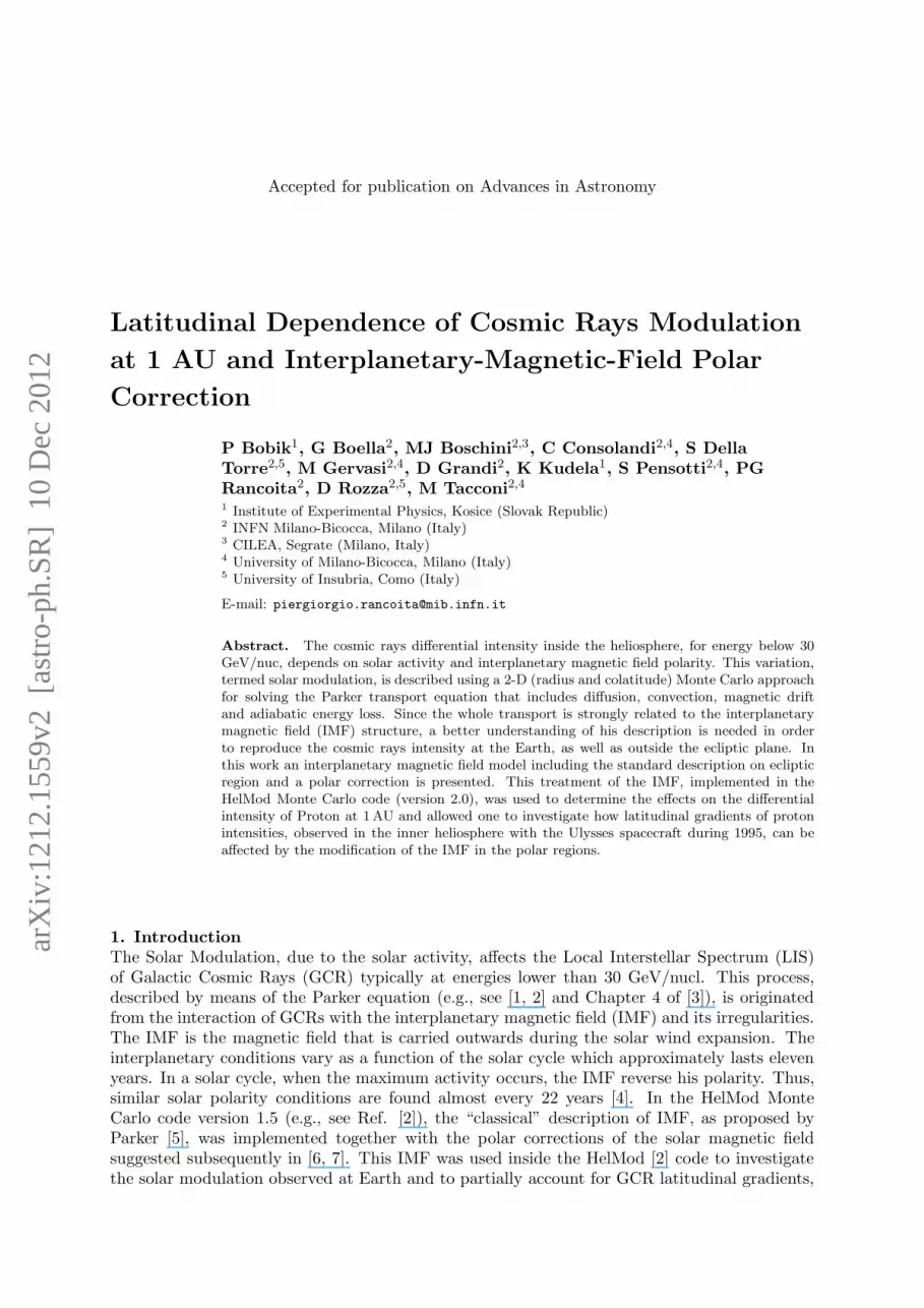
HelMod Energy bin KET channel(0.35 – 0.98) GeV (0.4 – 1.0)GeV(0.76 – 2.09) GeV (0.8 – 2.0)GeV(2.09 – 200)GeV > 2GeV

Table 2. Kinetic energy bins (in GeV) selected with HelMod Code and the correspondingproton energy channel for KET instruments on board the Ulysses spacecraft [8].

In order to have a divergence-free magnetic-field we require that the perturbation factor [δ(θ)]has to be:

δ(θ) =δm

[1− 2H (θ − θ′)] sin θ, (6)

where δm is the minimum perturbation factor of the field. The perturbation parameter is letto grow with decreasing of the colatitude. However, in their original work, Jokipii and Kota [6]estimated the value of the parameter δ between 10−3 and 3× 10−3.

Since the polar field is only a perturbation of the Parker field, it is a reasonable assumptionthat stream lines of the magnetic field do not cross the equatorial plane, thus, remainingcompletely contained in the solar hemisphere of injection. This allows one to estimate an upperlimit on the possible values of δm [see Fig. 1(b)]. Currently, we use δm = 1× 10−5 by comparingsimulations with observations at Earth orbit during Solar Cycle 23 (see Sect. 5).

Energy range θlat,min (in degrees)θ20◦ θ25◦ θ30◦

0.35 – 0.98 GeV −5+4−5 −8+4

−4 −9+3−3

0.76 – 2.09 GeV −5+6−7 −6+5

−6 −10+4−4

2.09 – 200 GeV −3+7−7 −7+7

−7 −9+5−6

Table 3. Latitudinal positions of minimum proton intensity (θlat,min) (in degrees) as a functionof the kinetic energy, using three values for the extension of the polar regions.

Energy range ∆N-S (%)θ20◦ θ25◦ θ30◦

0.35 – 0.98 GeV −8+6−6 −11+5

−4 −13+4−4

0.76 – 2.09 GeV −5+5−6 −6+5

−5 −9+3−3

2.09 – 200 GeV −1+3−1 −3+3

−3 −4+2−2

Table 4. Percentages of North-South asymmetry of proton intensities (∆N-S) as a function ofthe kinetic energy, using three values for the extension of the polar regions.

3. The Propagation Model

Parker in 1965 [1] (see also Ref. [2], Chapter 4 of [3] and references therein) treated thepropagation of GCRs trough the interplanetary space. He accounted for the so-called adiabaticenergy losses, outward convection due to the SW and drift effects. In the heliocentric system

– 5 –

Energy range ∆max (%)θ20◦ θ25◦ θ30◦

0.35 – 0.98 GeV −34+5−5 −35+4

−4 −36+4−3

0.76 – 2.09 GeV −22+6−7 −23+5

−4 −25+3−3

2.09 – 200 GeV −8+4−3 −9+3

−3 −10+2−2

Table 5. Differences in percentage between the maximum and minimum proton intensities(∆max) as a function of the kinetic energy, using three values for the extension of the polarregions.

the Parker equation is then expressed (e.g. see [2, 19]):

∂U

∂t=

∂

∂xi

(

KSij

∂U

∂xj

)

− ∂

∂xi[(Vsw,i + vd,i)U] +

1

3

∂Vsw,i

∂xi

∂

∂T(αrelTU) (7)

where U is the number density of particles per unit of particle kinetic energy T , at the timet. Vsw,i is the solar wind velocity along the axis xi [20], K

Sij is the symmetric part of diffusion

tensor [1], vd is the drift velocity that takes into account the drift of the particles due to thelarge scale structure of the magnetic field [21, 22, 23] and, finally,

αrel =T + 2mrc

2

T +mrc2,

where mr is the rest mass of the GCR particle. The last term of Eq. (7) accounts for adiabaticenergy losses [1, 24]. The number density U is related to the differential intensity J as ([2, 25],Chapter 4 of [3] and references therein):

J =vU

4π, (8)

where v is the speed of the GCR particle.Equation (7) was solved using the HelMod code (see the discussion in Ref. [2]). This treatment

(i) follows that introduced in Refs. [26, 27, 28, 29, 30, 10] and (ii) determines the differentialintensity of GCRs using a set of approximated stochastic differential equations (SDEs) whichprovides a solution equivalent to that from Eq. (7). The equivalence between the Parker equation,that is a Fokker-Planck type equation, and the SDEs is demonstrated in [28, 31]. In the presentwork, we use a 2D (radius and colatitude) approximation for the particle transport. The modelincludes the effects of solar activity during the propagation from the effective boundary of theheliosphere down to Earth’s position.

– 6 –

0.70

0.75

0.80

0.85

0.90

0.95

1.00

1.05

1.10

1.15 80° 60° 40° 20° 0° -20° -40° -60° -80° 80° 60° 40° 20° 0° -20° -40° -60° -80° 80° 60° 40° 20° 0° -20° -40° -60° -80°

0.70

0.75

0.80

0.85

0.90

0.95

1.00

1.05

1.10

1.15

0.65

0.70

0.75

0.80

0.85

0.90

0.95

1.00

1.05

1.10

1.15

Latitude

Nor

mal

ized

Inte

nsity

0.35 - 0.98 GeV20° 25°

Latitude

0.35 - 0.98 GeV 30°

Latitude

0.35 - 0.98 GeV

20°

Nor

mal

ized

Inte

nsity

0.76 - 2.09 GeV 25°

0.76 - 2.09 GeV 30°

0.76 - 2.09 GeV

20°

Nor

mal

ized

Inte

nsity

>2.09 GeV

0° 20° 40° 60° 80° 100°120°140°160°Colatitude

25°

>2.09 GeV

0° 20° 40° 60° 80° 100°120°140°160°Colatitude

30°

>2.09 GeV

0° 20° 40° 60° 80° 100°120°140°160°180°Colatitude

Figure 2. Latitudinal relative intensity at r =1AU, obtained at different solar colatitudes forprotons in the energy range defined in the Table 2 and using three definitions of polar regions:θ20◦ , θ25◦ and θ30◦ .

The set of SDEs for the 2D approximation of Eq. (7) in heliocentric spherical coordinates is

∆r =1

r2∂

∂r(r2KS

rr)∆t− ∂

∂µ(θ)

[

KSrµ

√

1− µ2(θ)

r

]

∆t

+(Vsw + vd,r)∆t+(

2KSrr

)1/2ωr

√∆t, (9a)

∆µ(θ) = − 1

r2∂

∂r

[

rKSµr

√

1− µ2(θ)]

∆t+∂

∂µ(θ)

[

KSµµ

1− µ2(θ)

r2

]

∆t

−1

rvd,µ

√

1− µ2(θ)∆t−2KS

rµ

r

[

1− µ2(θ)

2KSrr

]1/2

ωr

√∆t

+1

r

{

[1− µ2(θ)]KS

µµKSrr − (KS

rµ)2

0.5KSrr

}1/2

ωµ

√∆t, (9b)

∆T = −αrelT

3r2∂Vswr

2

∂r∆t, (9c)

– 7 –

0.700.750.800.850.900.951.001.051.101.15 80° 60° 40° 20° 0° -20° -40° -60° -80°

0.700.750.800.850.900.951.001.051.101.15

0.650.700.750.800.850.900.951.001.051.101.15

0.35 - 0.98 GeV

Latitude

Nor

mal

ized

Inte

nsity

0.76 - 2.09 GeV

Nor

mal

ized

Inte

nsity

30°

>2.09 GeV

R,0°

R,1°

R,2°

Nor

mal

ized

Inte

nsity

Colatitude0° 20° 40° 60° 80° 100° 120° 140° 160° 180°

Figure 3. For the polar regions θ < 30◦ and θ > 150◦, latitudinal relative intensity at r =1AU,accounting for GCR particles with 0◦ < θ < 180◦ (θR,0), 1

◦ < θ < 179◦ (θR,1) and 2◦ < θ < 178◦

(θR,2), respectively, are shown as a function of the proton kinetic energy and solar colatitude.Results with 10◦ < θ < 170◦ (θR,10) are comparable with those obtained with θR,2.

– 8 –

where µ(θ) = cos θ and ωi is a random number following a Gaussian distribution with a meanof zero and a standard deviation of one. The procedure for determining the SDEs can be foundin [2].

In a coordinate system with one axis parallel to the average magnetic field and the other twoperpendicular to this the symmetric part of the diffusion tensor KS

ij is (see e.g. [32]):

KSij =

K|| 0 00 K⊥,r 00 0 K⊥,θ

(10)

with K|| the diffusion coefficient describing the diffusion parallel to the average magnetic field,and K⊥,r and K⊥,θ are the diffusion coefficients describing the diffusion perpendicular to theaverage magnetic field in the radial and polar directions, respectively. In this work K|| is thatone proposed by Strauss and collaborators in Ref. [10] (see also [33, 34, 35]):

K|| =β

3K0

P

1GV

(

1 +r

1 AU

)

, (11)

where K0 is the diffusion parameter - described in Section 2.1 of [2] -, which depends on solaractivity and polarity, β is the particle speed in unit of speed of light, P = pc/|Z|e is the particlerigidity expressed in GV and, finally, r is the heliocentric distance from the Sun in AU.

In the current treatment, K|| has a radial dependence proportional to r, but no latitudinaldependence. Mc Donald and collaborators (see Ref. [36]) remarked that i) a spatial dependenceof K|| - like the one proposed here - can affect the latitudinal gradients at high latitude andii) it is consistent with that originally suggested in Ref. [6]. Furthermore, the perpendiculardiffusion coefficient is taken to be proportional to K|| with a ratio K⊥,i/K|| = 0.13 for both rand θ i-coordinates. The latter value is discussed in Sect. 5.

In addition, the practical relationship between K0 and monthly Smoothed Sunspot Numbers(SSN) [37] values - discussed in Section 2.1 of [2] - is currently updated using the most recentdata from Ref. [38]. As in Ref. [2], the K0 data are subdivided into four sets, i.e., ascending anddescending phases for both negative and positive solar magnetic-field polarities (Table 1). It hasto be remarked that after each maximum the sign of the magnetic field (i.e., the A parameterin Eq. (5)) is reversed. The updated practical relationships between K0 in AU2GV−1 s−1 andSSN values for 1.4 ≤SSN≤ 165 for the four periods (from I up to IV, listed in Table 1) are

I) K0 = 0.000297−2.9·10−6SSN+8.1·10−9SSN2+1.46·10−10SSN3−8.4·10−13SSN4 (12a)

II) K0 =

{

0.000304846 − 5.8 · 10−6SSN if SSN <= 200.00195SSN

− 2.3 · 10−10SSN2 + 9.1 · 10−5 if SSN > 20(12b)

III) K0 = 0.0002391 − 8.453 · 10−7SSN (12c)

IV) K0 = 0.000247 − 1.175 · 10−6SSN. (12d)

The rms (root mean square) values of the percentage difference between values obtained withEqs. (12) from those determined using the procedure discussed in Section 2.1 of [2] applied to thedata from Ref. [38] were found to be 6.0%, 10.1%, 7.0% and 13.2% for the period I (ascendingphase with A < 0), II (descending phase with A < 0), III (ascending phase with A > 0) and IV(descending phase with A > 0), respectively.

4. The Magnetic Field in the Polar Regions

Section 2 describes an IMF following the Parker Field with a small region around the polesin which such a field is modified. As already mentioned (see e.g.[6, 39, 40, 41, 42, 43]), thecorrection is needed to better reproduce the complexity of the magnetic field in those regions.

– 9 –

δm (×10−5) ρk “R” model “L” model No Drift0.0 0.10 14.1 11.0 33.41.0 0.10 11.7 8.7 33.22.0 0.10 11.6 8.3 33.73.0 0.10 11.6 8.3 33.71.0 0.11 6.4 9.0 27.72.0 0.11 7.8 9.0 28.33.0 0.11 7.5 8.8 29.21.0 0.12 6.3 7.1 23.52.0 0.12 6.3 7.3 24.73.0 0.12 7.1 6.9 24.41.0 0.13 6.3 6.4 20.12.0 0.13 6.6 7.6 20.43.0 0.13 6.7 7.7 20.51.0 0.14 7.3 7.0 15.92.0 0.14 7.3 7.2 16.43.0 0.14 7.2 6.5 16.8

Table 6. Average values (last three columns) of ηrms (in percentage, %) as a function ofδm (×10−5) and ρk, for BESS–1997, AMS–1998, PAMELA-2006/08, obtained from Eq. (16)without enhancement of the diffusion tensor along the polar direction (ρE = 1), using “R” and“L” models for the tilt angle and No Drift approximation. The differential intensities werecalculated accounting for particles inside the heliospheric regions for which solar latitudes arelower than |5.7◦|.

Moreover, Ulysses spacecraft (see e.g. [44, 45, 46]) explored the heliosphere outside the eclipticplane up to ±80◦ of solar latitude at a solar distance from ∼ 1 up to ∼ 5AU. Using theseobservations, the presence of latitudinal gradient in the proton intensity could be determined(e.g., see Figure 2 of Ref. [9] and Figure 5 of Ref. [8]). The data collected during the latitudinalfast scan (from September 1994 up to August 1995) show (a) a nearly symmetric latitudinalgradient with the minimum near ecliptic plane, (b) a southward shift of the minimum and(c) an intensity in the North polar region at 80◦ exceeding the South polar intensity. In Ref.[9] a latitudinal gradient of ∼ 0.3%/degree for proton with kinetic energy > 0.1 GeV wasestimated. While in Ref. [8] the analysis to higher energy was extended estimating a gradientof ∼ 0.22%/degree for proton with kinetic energy > 2 GeV. The minimum in the chargedparticle intensity separating the two hemispheres of the heliosphere occurs ∼ 10◦ South ofthe heliographic equator [9]. In addition, an independent analysis that takes into account thelatitudinal motion of the Earth and IMP8 confirms a significant (∼ 8◦ ± 2◦) southward offset ofthe intensity minimum [9] for T > 100 MeV proton. Furthermore in Ref. [8], a southward offsetof about ≈ 7◦ is evaluated; this offset of the intensity minimum results to be independent of theparticle energy up to 2 GeV. Finally, in Ref. [9], the intensity in the North polar region at 80◦

is observed to exceed the South polar intensity of ∼ 6% for protons with T > 100 MeV.Using the present HelMod code (version 2.0), we could investigate i) the latitudinal gradient

of GCR intensities resulting from solar modulation and ii) how the magnetic-field structure ofthe polar regions, as defined in Sect. 2, is able to influence the GCR spectra on the ecliptic plane.As previously defined, we denote with θX◦ a polar region of amplitude X◦ from polar axis, i.e.,θ < X◦ and θ > 180◦ − X◦. Three regions with X◦ = 20◦, 25◦ and 30◦ were investigated.Outside any of these regions, the ratio between BPol and BPar in Eq. (5) is less than ∼1% (seeFig. 1) and, thus, it ensures a smooth transition between polar and equatorial regions. For the

– 10 –

10-1 100 10110-1

100

101

102

103

104

105

Diff

eren

tial i

nten

sity

Kinetic energy

[(m2 s

r s G

eV)-1

]

[GeV]

LIS

BESS-1997

Modulated spectra

Figure 4. Proton differential intensity determined with the HelMod code (continuous line)compared to the experimental data of BESS–1997; the dashed line is the LIS (see the text).

purpose or this study we consider an energy binning closer to those presented in Ref. [8]. TheKET instrument [47] collects proton data in three “channels” one with energies ranging from0.038GeV up to 2.0GeV and two for particle with kinetic energy T > 0.1 GeV and T > 2 GeV,respectively. A successive re-analysis of the collected data allowed the authors to subdividethe 0.25–2 GeV “channel” in three “sub-channels” of intermediate energies. Since the PresentModel is optimized - as discussed in Ref. [2] - for particles with rigidity greater than 1GV(i.e., ≈ 0.444GeV), the present results are compared only with the corresponding “channel” or“sub-channels” suited for the corresponding energy range (see Table 2).

At 1AU and as a function of the solar colatitude, the GCR intensities for protons are shownin Fig. 2. For a comparison with Ulysses observations, the modulated intensities of protons -resulting from HelMod code - were investigated from 80◦ (North) and down to −80◦ (South).They were obtained using the HelMod code and selected using the energy bins reported in table2. In Fig. 2, the latitudinal intensity distribution is normalized to the corresponding South Poleintensity. The quoted errors include statistical and systematic errors. The distributions wereinterpolated using a parabolic function expressed as:

I(θlat) = a+ c(θlat + d)2, (13)

where I(θlat) is the normalized intensity, θlat is the latitudinal angle1 and a, b and c areparameters determined from the fitting procedure. The so obtained fitted curves are shown ascontinuous lines in Fig. 2. Furthermore, the latitudinal positions of minimum intensity (θlat,min),

1 The latitudinal angle is θlat = 90◦ − θ.

– 11 –

10-1 100 10110-1

100

101

102

103

104

105

Diff

eren

tial i

nten

tsity

Kinetic energy

[(m2 s

r s G

eV)-1

]

[GeV]

LIS

AMS-1998

Modulated spectra

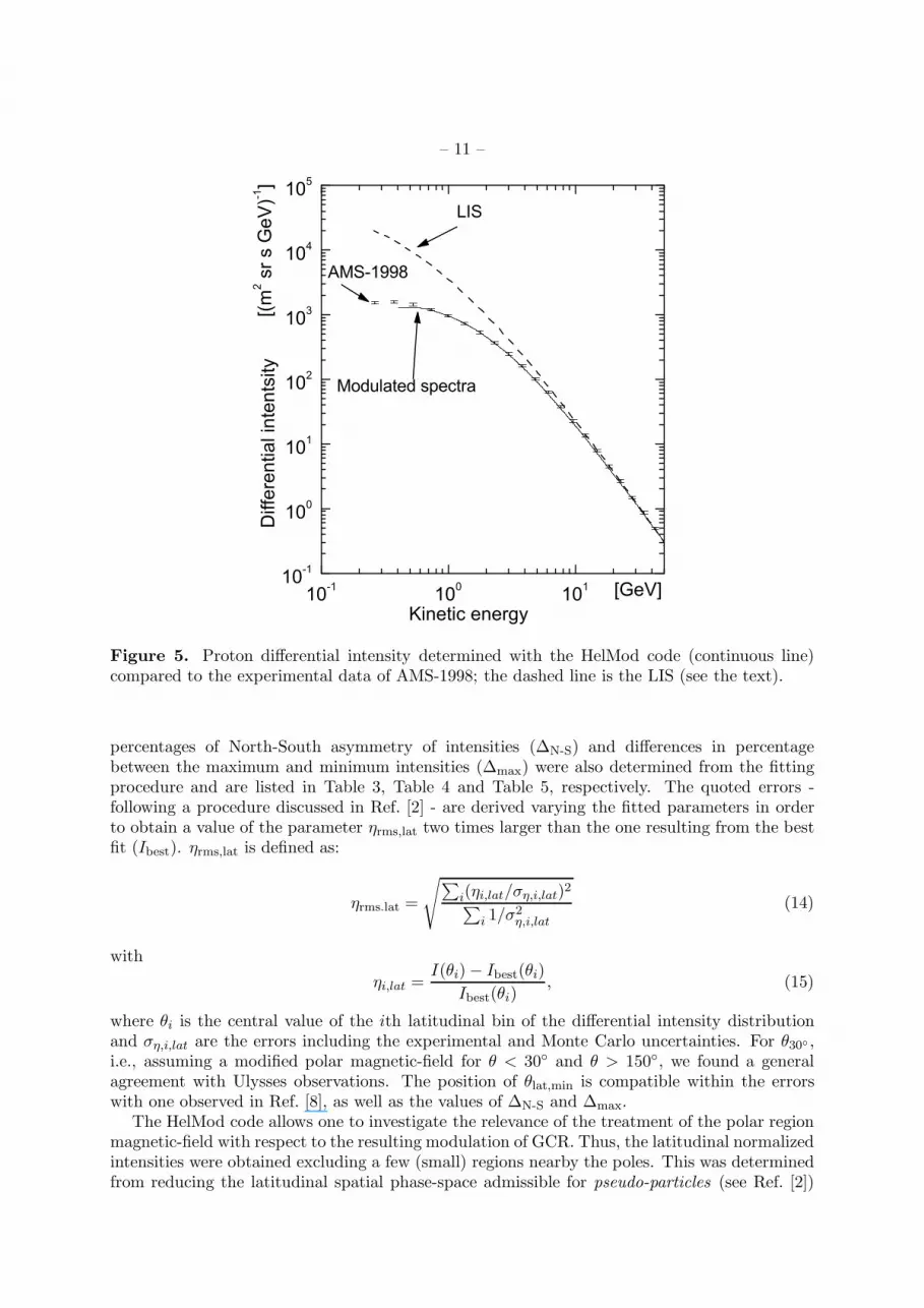
Figure 5. Proton differential intensity determined with the HelMod code (continuous line)compared to the experimental data of AMS-1998; the dashed line is the LIS (see the text).

percentages of North-South asymmetry of intensities (∆N-S) and differences in percentagebetween the maximum and minimum intensities (∆max) were also determined from the fittingprocedure and are listed in Table 3, Table 4 and Table 5, respectively. The quoted errors -following a procedure discussed in Ref. [2] - are derived varying the fitted parameters in orderto obtain a value of the parameter ηrms,lat two times larger than the one resulting from the bestfit (Ibest). ηrms,lat is defined as:

ηrms.lat =

√

∑

i(ηi,lat/ση,i,lat)2

∑

i 1/σ2η,i,lat

(14)

with

ηi,lat =I(θi)− Ibest(θi)

Ibest(θi), (15)

where θi is the central value of the ith latitudinal bin of the differential intensity distributionand ση,i,lat are the errors including the experimental and Monte Carlo uncertainties. For θ30◦ ,i.e., assuming a modified polar magnetic-field for θ < 30◦ and θ > 150◦, we found a generalagreement with Ulysses observations. The position of θlat,min is compatible within the errorswith one observed in Ref. [8], as well as the values of ∆N-S and ∆max.

The HelMod code allows one to investigate the relevance of the treatment of the polar regionmagnetic-field with respect to the resulting modulation of GCR. Thus, the latitudinal normalizedintensities were obtained excluding a few (small) regions nearby the poles. This was determinedfrom reducing the latitudinal spatial phase-space admissible for pseudo-particles (see Ref. [2])

– 12 –

10-1 100 10110-1

100

101

102

103

104

105

Diff

eren

tial i

nten

sity

Kinetic energy

[(m2 s

r s G

eV)-1

]

[GeV]

LIS

PAMELA-2006/08

Modulated spectra

Figure 6. Proton differential intensity determined with the HelMod code (continuous line)compared to the experimental data of PAMELA 2006/08; the dashed line is the LIS (see thetext).

- i.e., the latitudinal extension of GCR particles taken into account - to 1◦ < θ < 179◦ (θR,1),2◦ < θ < 178◦ (θR,2) and 10◦ < θ < 170◦ (θR,10). The so obtained latitudinal gradients arecompared with the full latitudinal extension, θR,0 (0◦ < θ < 180◦), in Fig. 3. By an inspectionof Fig. 3, one may lead to the conclusion that the GCR diffusion nearby the polar axis has alarge impact on the latitudinal gradients in the inner heliosphere. As a consequence, the IMFdescription in the polar regions is relevant in order to reproduce the observed modulated GCRspectra.

5. Comparison with Observations During Solar Cycle 23

The agreement of HelMod simulated spectra with observations during solar cycle 23 isinvestigated via quantitative comparisons using Eqs. (16) and (17). However, since the structureof the heliosphere is different in high and low solar activity the two periods are separatelyanalyzed.

The HelMod Code [2] (version 2.0) allowed us to investigate how the modulated (simulated)differential intensities are affected by the (1) particle drift effect, (2) polar enhancement of thediffusion tensor along the polar direction (K⊥,θ, e.g., see Ref. [48]), and, finally, (3) values of thetilt angle (αt) calculated following the approach of the “R” and “L” models [49]. This analysisalso allow us to estimate the values of IMF parameters that better describe the modulationalong the entire solar cycle. The effects related to particle drift were investigated via thesuppression of the drift velocity (No Drift approximation), this accounts for the hypothesisthat magnetic drift convection is almost completely suppressed during solar maxima. The

– 13 –

δm (×10−5) ρk “R” model “L” model No Drift0.0 0.10 11.2 10.8 15.41.0 0.10 11.0 10.1 15.82.0 0.10 9.6 10.0 16.73.0 0.10 9.6 10.0 16.71.0 0.11 13.4 13.1 16.02.0 0.11 12.7 12.9 15.43.0 0.11 12.7 12.5 16.21.0 0.12 18.7 17.7 13.42.0 0.12 18.3 16.9 12.83.0 0.12 18.1 17.3 12.81.0 0.13 23.3 23.5 14.32.0 0.13 25.0 24.7 13.33.0 0.13 24.3 24.2 13.11.0 0.14 32.3 30.7 18.02.0 0.14 32.8 30.8 17.13.0 0.14 31.5 30.7 17.9

Table 7. Average values (last three columns) of ηrms (in percentage, %) as a function ofδm (×10−5) and ρk, for BESS–1999, BESS–2000, BESS–2002, obtained from Eq. (16) withoutenhancement of the diffusion tensor along the polar direction (ρE = 1), using “R” and “L”models for the tilt angle and No Drift approximation. The differential intensities were calculatedaccounting for particles inside the heliospheric regions for which solar latitudes are lower than|5.7◦|.

differential intensities were calculated for K⊥,µ = ρEK⊥,r with values of ρE of 1, 8 and 10,i.e., no enhancement, that suggested in Ref. [50] and that suggested in Ref. [48, 2] (andreference there in), respectively. Furthermore, the modulated proton spectra were derived froma LIS whose normalization constant depends on the experimental set of data and were alreadydiscussed in Ref. [2]). In addition, the differential intensities were calculated accounting forparticles inside heliospheric regions where solar latitudes are lower than |5.7◦|.

During the period of high solar activity for the solar cycle 23, the BESS collaboration tookdata in the years 1999, 2000, and 2002 (see sets of data in Ref. [51]). For period not dominatedby high solar activity in solar cycle 23, BESS, AMS and PAMELA collaborations took data,i.e., BESS–1997 [51], AMS–1998 [52], and PAMELA–2006/08 [53].

Following the procedure described in Ref. [2], the observation data were compared with thoseobtained from HelMod code using the error-weighted root mean square (ηrms) of the relativedifference (η) between experimental data (fexp) and those resulting from simulated differentialintensities (fsim). For each set of experimental data and with the approximations and/or modelsdescribed above, we determined the quantity

ηrms =

√

∑

i(ηi/ση,i)2

∑

i 1/σ2η,i

(16)

with

ηi =fsim(Ti)− fexp(Ti)

fref(Ti), (17)

where Ti is the average energy of the ith energy bin of the differential intensity distribution andση,i are the errors including the experimental and Monte Carlo uncertainties; the latter account

– 14 –

10-1 100 10110-1

100

101

102

103

104

105

Diff

eren

tial i

nten

sity

Kinetic energy

[(m2 s

r s G

eV)-1

]

[GeV]

LIS

BESS-1999

Modulated spectra

Figure 7. Proton differential intensity determined with the HelMod code (continuous line)compared to the experimental data of BESS–1999; the dashed line is the LIS (see the text).

for the Poisson error of each energy bin. The simulated differential intensities are interpolatedwith a cubic spline function. The modulation results are studied varying the parameters δm -from 0, i.e., the non-modified Parker IMF, up to 3× 10−5, see Fig. 1(b) -, K⊥,r/K|| = ρk (from0.10 up to 0.14) and K⊥,θ/K⊥,r = ρE (from 1 up to 10) seeking a set of parameters set thatminimize ηrms. In Table 6, the average values of ηrms (in percentage, %) for low solar activityperiods are listed. They were obtained in the energy range 2 from 444 MeV up to 30 GeV usingthe “L” and “R” models for the tilt angle αt and for the No Drift approximation and withoutany enhancement of the diffusion tensor along the polar direction (K⊥,µ). The results derivedwith the enhancement of the diffusion tensor along the polar direction indicate that for ρE = 8and 10 one obtains a value of ηrms that is from 1.5 up to 3 times larger with respect the casewithout enhancement3. From inspection of Table 6, one can remark that the drift mechanismleads to a better agreement with experimental data. Furthermore the, “R” and “L” modelsfor tilt angles are comparable within the precision of the method (discussed in Ref. [2]). Theminimum difference with respect to the experimental data occurs when ρk = 0.11 − 0.13 andδm = 1.0× 10−5 for both “R” and “L” models, with the “L” model slightly preferred to “R”.

In Figs. 4–6, the differential intensities determined with the HelMod code are shownand compared to the experimental data of BESS–1997, AMS–1998, and PAMELA–2006/08,respectively; in these figures, the dashed lines are the LIS as discussed in Ref. [2]. Thesemodulated intensities are the ones calculated for a heliospheric region where solar latitudes are

2 Above 30GeV, the differential intensity is marginally (if at all) affected by modulation.3 For a comparison, the scalar approximation presented in Ref. [2], i.e., assuming that the diffusion propagationis independent of magnetic structure, leads to and average ηrms of ∼ 15%.

– 15 –

10-1 100 10110-1

100

101

102

103

104

105

Diff

eren

tial i

nten

sity

Kinetic energy

[(m2 s

r s G

eV)-1

]

[GeV]

LIS

BESS-2000

Modulated spectra

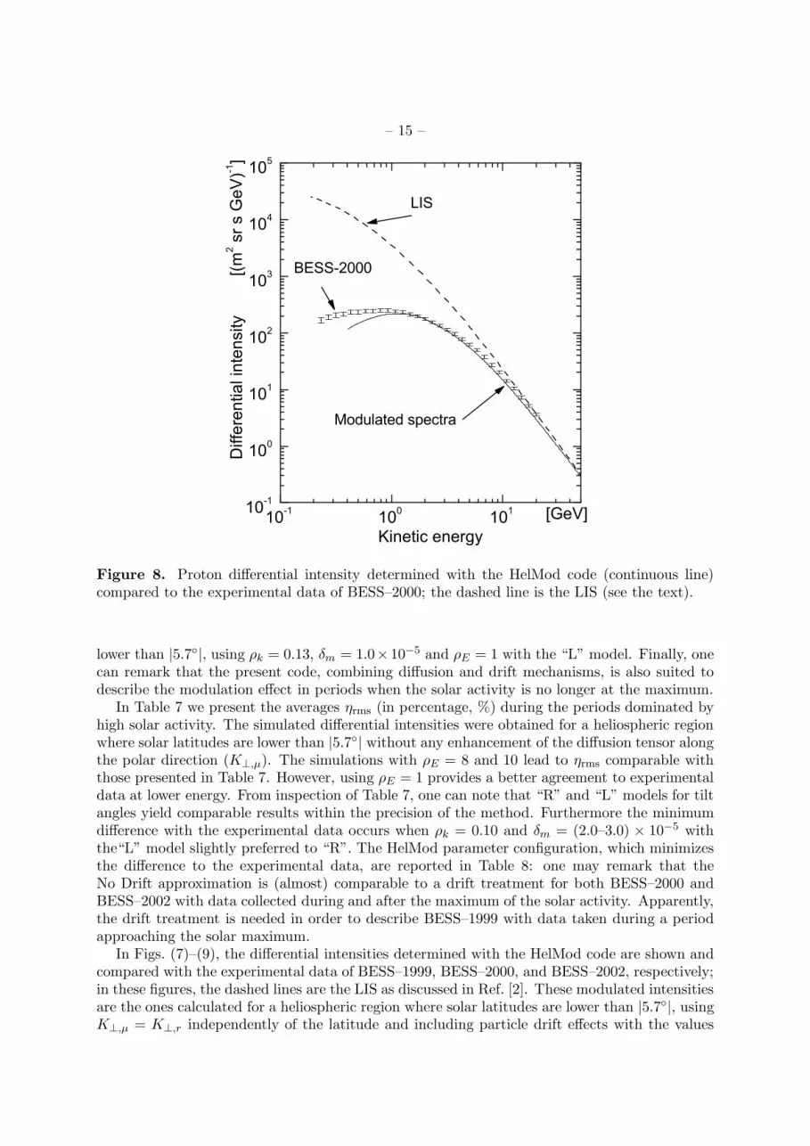
Figure 8. Proton differential intensity determined with the HelMod code (continuous line)compared to the experimental data of BESS–2000; the dashed line is the LIS (see the text).

lower than |5.7◦|, using ρk = 0.13, δm = 1.0×10−5 and ρE = 1 with the “L” model. Finally, onecan remark that the present code, combining diffusion and drift mechanisms, is also suited todescribe the modulation effect in periods when the solar activity is no longer at the maximum.

In Table 7 we present the averages ηrms (in percentage, %) during the periods dominated byhigh solar activity. The simulated differential intensities were obtained for a heliospheric regionwhere solar latitudes are lower than |5.7◦| without any enhancement of the diffusion tensor alongthe polar direction (K⊥,µ). The simulations with ρE = 8 and 10 lead to ηrms comparable withthose presented in Table 7. However, using ρE = 1 provides a better agreement to experimentaldata at lower energy. From inspection of Table 7, one can note that “R” and “L” models for tiltangles yield comparable results within the precision of the method. Furthermore the minimumdifference with the experimental data occurs when ρk = 0.10 and δm = (2.0–3.0) × 10−5 withthe“L” model slightly preferred to “R”. The HelMod parameter configuration, which minimizesthe difference to the experimental data, are reported in Table 8: one may remark that theNo Drift approximation is (almost) comparable to a drift treatment for both BESS–2000 andBESS–2002 with data collected during and after the maximum of the solar activity. Apparently,the drift treatment is needed in order to describe BESS–1999 with data taken during a periodapproaching the solar maximum.

In Figs. (7)–(9), the differential intensities determined with the HelMod code are shown andcompared with the experimental data of BESS–1999, BESS–2000, and BESS–2002, respectively;in these figures, the dashed lines are the LIS as discussed in Ref. [2]. These modulated intensitiesare the ones calculated for a heliospheric region where solar latitudes are lower than |5.7◦|, usingK⊥,µ = K⊥,r independently of the latitude and including particle drift effects with the values

– 16 –

10-1 100 10110-1

100

101

102

103

104

105

Diff

eren

tial i

nten

sity

Kinetic energy

[(m2 s

r s G

eV)-1

]

[GeV]

LIS

BESS-2002

Modulated spectra

Figure 9. Proton differential intensity determined with the HelMod code (continuous line)compared to the experimental data of BESS–2002; the dashed line is the LIS (see the text).

Observations “R” model “L” model No DriftBESS–1999 9.3 10.6 25.7BESS–2000 12.5 12.6 16.7BESS–2002 6.9 6.7 7.7

Table 8. Average ηrms (in percentage, %), for BESS–1999, BESS–2000, BESS–2002, obtainedfrom Eq. (16) without enhancement of the diffusion tensor along the polar direction (ρE = 1),δm = 2.0 × 10−5, ρk = 0.10 and using “R” and “L” models for the tilt angle and No Driftapproximation. The differential intensities were calculated accounting for particles inside theheliospheric regions for which solar latitudes are lower than |5.7◦|.

of the tilt angle from the “L” model. Finally, it is concluded that the present code combiningdiffusion and drift mechanisms is suited to describe the modulation effect in periods with highsolar activity [2, 50, 54].

6. Conclusion

In this work an IMF, which combines the Parker Field and its polar modification, is presented.In the polar regions, the Parker IMF was modified with an additional latitudinal componentsaccording to those proposed by Jokipii and Kota in Ref. [6]. We found the maximum perturbedvalue with this component yielding, as a physical result, streaming lines completely confined inthe solar hemisphere of injection.

The proposed IMF is, then, used within the HelMod Monte Carlo code to determine the

– 17 –

effects on the differential intensity of protons at 1AU as a function of the extension of polarregion, in which the modified magnetic-field is employed. We found that a polar region containedwithin 30◦ of colatitude is that one ensuring a very smooth transition to the equatorial region andallows to reproduce qualitatively and quantitatively the latitudinal profile of the GCR intensity,and the latitudinal dip shift with respect to the ecliptic plane. Finally we determined how thepolar region diffusion is mostly responsible of the proton intensity latitudinal gradient observedin the inner heliosphere with the Ulysses spacecraft during 1995.

Acknowledgements

KK wishes to acknowledge VEGA grant agency project 2/0081/10 for support. Finally, theauthors acknowledge the use of NASA/GSFC’s Space Physics Data Facility’s OMNIWeb service,and OMNI data.

References[1] E. N. Parker. The passage of energetic charged particles through interplanetary space. Plan. Space Sci.,

13:9, 1965.[2] P. Bobik, G. Boella, M. J. Boschini, C. Consolandi, S. Della Torre, M. Gervasi, D. Grandi, K. Kudela,

S. Pensotti, P. G. Rancoita, and M. Tacconi. Systematic Investigation of Solar Modulation of GalacticProtons for Solar Cycle 23 Using a Monte Carlo Approach with Particle Drift Effects and LatitudinalDependence. Astrophys. J., 745:132, February 2012.

[3] C. Leroy and P.-G. Rancoita. Principles of Radiation Interaction in Matter and Detection, 3rd Edition.World Scientific Publishing Co, 2011.

[4] R. D. Strauss, M. S. Potgieter, and S. E. S. Ferreira. Modeling ground and space based cosmic rayobservations. Adv. Space Res., 49:392–407, January 2012.

[5] E. N. Parker. Dynamics of the interplanetary gas and magnetic fields. Astrophys. J., 128:664, 11 1958.[6] J. R. Jokipii and J. Kota. The polar heliospheric magnetic field. Geophys. Res. Lett., 16:1–4, Jan 1989.[7] U.W. Langner. Effect of termination shock acceleraion on cosmic ray in the helisphere. PhD thesis,

Potchestroom University, Potchestroom, 2004.[8] B. Heber, W. Droege, P. Ferrando, L. J. Haasbroek, H. Kunow, R. Mueller-Mellin, C. Paizis, M. S. Potgieter,

A. Raviart, and G. Wibberenz. Spatial variation of >40MeV/n nuclei fluxes observed during the ULYSSESrapid latitude scan. Astron. Astrophys., 316:538–546, December 1996.

[9] J. A. Simpson. Ulysses cosmic-ray investigations extending from the south to the north polar regions of theSun and heliosphere. Nuovo Cimento C, 19:935–943, December 1996.

[10] R. D. Strauss, M. S. Potgieter, I. Busching, and A. Kopp. Modeling the Modulation of Galactic and JovianElectrons by Stochastic Processes. Astrophys. J., 735:83, July 2011.

[11] E. N. Parker. Newtonian Development of the Dynamical Properties of Ionized Gases of Low Density. Phys.

Rev., 107:924–933, August 1957.[12] E. N. Parker. The Hydrodynamic Theory of Solar Corpuscular Radiation and Stellar Winds. Astrophys. J.,

132:821, November 1960.[13] E. N. Parker. Sudden Expansion of the Corona Following a Large Solar Flare and the Attendant Magnetic

Field and Cosmic-Ray Effects. Astrophys. J., 133:1014, May 1961.[14] E. N. Parker. Interplanetary dynamical processes. New York, Interscience Publishers, 1963., 1963.[15] M. Hattingh and R. A. Burger. A new simulated wavy neutral sheet drift model. Adv. Space Res., 16(9):213–

216, 1995.[16] J. H. King and N. E. Papitashvili. Solar wind spatial scales in and comparisons of hourly Wind and ACE

plasma and magnetic field data. J. Geophys. Res.-Space, 110(A9):A02104, February 2005.[17] NASA-OMNIweb. online database http://omniweb.gsfc.nasa.gov/form/dx1.html, 2012.[18] J. R. Jokipii and B. Thomas. Effects of drift on the transport of cosmic rays. IV - Modulation by a wavy

interplanetary current sheet. Astrophys. J., 243:1115–1122, February 1981.[19] J. R. Jokipii, E. H. Levy, and W. B. Hubbard. Effect of particle drift on cosmic-ray transport. i. general

properties, application to solar modulation. Astrophys. J. Lett., 213:L85–L88, April 1977.[20] E. Marsch, W. I. Axford, and J. F. McKenzie. Solar wind. In B. N. Dwivedi, editor, Dynamic Sun, pages

374–402, 2003.[21] J. R. Jokipii and E. H. Levy. Effects of particle drifts on the solar modulation of galactic cosmic rays.

Astrophys. J. Lett., 213:L85–L88, April 1977.

– 18 –

[22] M. S. Potgieter and H. Moraal. A drift model for the modulation of galactic cosmic rays. Astrophys. J.,294(part 1):425–440, 1985.

[23] R. A. Burger and M. Hattingh. Steady-State Drift-Dominated Modulation Models for Galactic Cosmic Rays.Astroph. and Sp. Sc., 230:375–382, August 1995.

[24] J. R. Jokipii and E. N. Parker. On the Convection, Diffusion, and Adiabatic Deceleration of Cosmic Raysin the Solar Wind. Astroph. J., 160:735, May 1970.

[25] L. J. Gleeson and W. I. Axford. Solar Modulation of Galactic Cosmic Rays. Astrophys. J., 154:1011,December 1968.

[26] Y. Yamada, S. Yanagita, and T. Yoshida. A stochastic view of the solar modulation phenomena of cosmicrays. Geophys. Res. Lett., 25:2353–2356, July 1998.

[27] M. Gervasi, P. G. Rancoita, I. G. Usoskin, and G. A. Kovaltsov. Monte-Carlo approach to Galactic CosmicRay propagation in the Heliosphere. Nucl. Phys. B - Proc. Sup., 78:26–31, August 1999.

[28] M. Zhang. A Markov Stochastic Process Theory of Cosmic-Ray Modulation. Astrophys. J., 513:409–420,March 1999.

[29] K. Alanko-Huotari, I. G. Usoskin, K. Mursula, and G. A. Kovaltsov. Stochastic simulation of cosmic raymodulation including a wavy heliospheric current sheet. J. Geophys. Res., 112:A08101, 2007.

[30] C. Pei, J. W. Bieber, R. A. Burger, and J. Clem. A general time-dependent stochastic method for solvingParker’s transport equation in spherical coordinates. J. Geophys. Res.-Space, 115(A12107), December2010.

[31] C.W. Gardiner. Handbook of stochastic methods: for physics, chemistry and natural sciences. SpringerEdition, 1985.

[32] J. R. Jokipii. Propagation of cosmic rays in the solar wind. Rev. Geoph. Space Phys., 9:27–87, 1971.[33] I. D. Palmer. Transport coefficients of low-energy cosmic rays in interplanetary space. Rev. Geophys. Space

Ge., 20:335–351, May 1982.[34] M. S. Potgieter and S. E. S. Ferreira. Effects of the solar wind termination shock on the modulation of

Jovian and galactic electrons in the heliosphere. J. Geophys. Res.-Space, 107:1089, July 2002.[35] W. Droge. Probing heliospheric diffusion coefficients with solar energetic particles. Adv. Space Res., 35:532–

542, 2005.[36] F. B. McDonald, P. Ferrando, B. Heber, H. Kunow, R. McGuire, R. Muller-Mellin, C. Paizis, A. Raviart,

and G. Wibberenz. A comparative study of cosmic ray radial and latitudinal gradients in the inner andouter heliosphere. J. Geophys. Res., 102:4643–4652, March 1997.

[37] SIDC-team. The International Sunspot Number. Monthly Report on the International Sunspot Number,

online catalogue, 1964-2010.[38] I. G. Usoskin, G. A. Bazilevskaya, and G. A. Kovaltsov. Solar modulation parameter for cosmic rays since

1936 reconstructed from ground-based neutron monitors and ionization chambers. J. Geophys. Res.-Space,116:A02104, February 2011.

[39] A. Balogh, E. J. Smith, B. T. Tsurutani, D. J. Southwood, R. J. Forsyth, and T. S. Horbury. The HeliosphericMagnetic Field Over the South Polar Region of the Sun. Science, 268:1007–1010, May 1995.

[40] H. Moraal. Proton Modulation Near Solar Minimim Periods in Consecutive Solar Cycles. In International

Cosmic Ray Conference, volume 6, page 140, 1990.[41] C. W. Smith and J. W. Bieber. Solar cycle variation of the interplanetary magnetic field spiral. Astroph.

J., 370:435–441, March 1991.[42] L. A. Fisk. Motion of the footpoints of heliospheric magnetic field lines at the Sun: Implications for recurrent

energetic particle events at high heliographic latitudes. J. Geophys. Res., 101:15547–15554, July 1996.[43] M. Hitge and R. A. Burger. Cosmic ray modulation with a Fisk-type heliospheric magnetic field and a

latitude-dependent solar wind speed. Adv. Space Res., 45:18–27, January 2010.[44] T. R. Sanderson, R. G. Marsden, K.-P. Wenzel, A. Balogh, R. J. Forsyth, and B. E. Goldstein. High-Latitude

Observations of Energetic Ions During the First ULYSSES Polar Pass. Space Sci. Rev., 72:291–296, April1995.

[45] R. G. Marsden. The 3-D Heliosphere at Solar Maximum. The Publications of the Astronomical Society of

the Pacific, 113:129–130, January 2001.[46] A. Balogh, R. G. Marsden, and E. J. Smith. The heliosphere near solar minimum. The Ulysses perspective.

Springer-Praxis Books in Astrophysics and Astronomy, 2001.[47] B. Heber, M. S. Potgieter, and P. Ferrando. Solar modulation of galactic cosmic rays: the 3D heliosphere.

Adv. Space Res., 19:795–804, May 1997.[48] M. S. Potgieter. Heliospheric modulation of cosmic ray protons: Role of enhanced perpendicular diffusion

during periods of minimum solar modulation. J. Geophys. Res., 105:18295–18304, 2000.[49] J. T. Hoeksema. The Large-Scale Structure of the Heliospheric Current Sheet During the ULYSSES Epoch.

Space Sci. Rev., 72:137–148, April 1995.

– 19 –

[50] S. E. S. Ferreira and M. S. Potgieter. Long-Term Cosmic-Ray Modulation in the Heliosphere. Astrophys.

J., 603:744–752, March 2004.[51] Y. Shikaze, S. Orito, T. Mitsui, and BESS Collaboration. Measurements of 0.2 20 GeV/n cosmic-ray proton

and helium spectra from 1997 through 2002 with the BESS spectrometer. Astrop. Phys., 28:154–167,2007.

[52] M. Aguilar, J. Alcaraz, J. Allaby, and AMS Collaboration. The Alpha Magnetic Spectrometer (AMS) onthe International Space Station: Part I - results from the test flight on the space shuttle. Phys. Rep.,366:331–405, 2002.

[53] O. Adriani, G. C. Barbarino, G. A. Bazilevskaya, and PAMELA Collaboration. PAMELA Measurements ofCosmic-Ray Proton and Helium Spectra. Science, 332:69, 2011.

[54] D. C. Ndiitwani, S. E. S. Ferreira, M. S. Potgieter, and B. Heber. Modelling cosmic ray intensities along theUlysses trajectory. Annales Geophysicae, 23:1061–1070, March 2005.