assessing circumbinary habitable zones using latitudinal

MNRAS 437, 1352–1361 (2014) doi:10.1093/mnras/stt1964Advance Access publication 2013 November 13

Assessing circumbinary habitable zones using latitudinal energy balancemodelling

Duncan Forgan‹

Scottish Universities Physics Alliance (SUPA), Institute for Astronomy, University of Edinburgh, Blackford Hill, Edinburgh EH9 3HJ, UK

Accepted 2013 October 11. Received 2013 September 23; in original form 2013 August 6

ABSTRACTPrevious attempts to describe circumbinary habitable zones (HZs) have been concerned withthe spatial extent of the zone, calculated analytically according to the combined radiationfield of both stars. By contrast to these ‘spatial HZs’, we present a numerical analysis ofthe ‘orbital HZ’, an HZ defined as a function of planet orbital elements. This orbital HZ isbetter equipped to handle (for example) eccentric planet orbits, and is more directly connectedto the data returned by exoplanet observations. Producing an orbital HZ requires a largenumber of climate simulations to be run to investigate the parameter space – we achieve thisusing latitudinal energy balance models, which handle the insolation of the planet by both stars(including mutual eclipses), as well as the planetary atmosphere’s ability to absorb, transfer andlose heat. We present orbital HZs for several known circumbinary planetary systems: Kepler-16, Kepler-34, Kepler-35, Kepler-47 and PH-1. Generally, the orbital HZs at zero eccentricityare consistent with spatial HZs derived by other authors, although we detect some signaturesof variability that coincide with resonances between the binary and planet orbital periods. Weconfirm that Earth-like planets around Kepler-47 with Kepler-47c’s orbital parameters couldpossess liquid water, despite current uncertainties regarding its eccentricity. Kepler-16b isfound to be outside the HZ, as well as the other circumbinary planets investigated.

Key words: astrobiology – methods: numerical – planets and satellites: general.

1 IN T RO D U C T I O N

The habitable zone (HZ) is a useful conceptual tool in investigatingthe general habitability of planetary systems. It is usually definedas the region surrounding a star within which, if a terrestrial planet ofEarth mass and similar atmospheric composition were to reside, thewater upon the planet’s surface would remain liquid (Huang 1959;Hart 1979). The boundaries of the HZ are subsequently definedby the properties of the host star: the outer boundary of the HZis typically governed by the rate at which CO2 clouds maintaina sufficiently strong greenhouse effect, and the inner edge of theHZ is controlled by the rate of water loss via hydrogen escape andhydrolysis. The HZ is sensitive to the spectrum of the source ofinsolation – in particular, how strongly the source emits in theinfrared (IR). As a result, the inner and outer boundaries of the HZare a function of the effective temperature of the star.

While the majority of the literature utilizing the HZ concept hasrelied on the seminal atmospheric radiative transfer calculations ofKasting, Whitmire & Reynolds (1993), and subsequent parametriza-tions (e.g. Underwood, Jones & Sleep 2003; Selsis et al. 2007;

� E-mail: [email protected]

Kaltenegger & Sasselov 2011), it should be noted that Kopparapuet al. (2013) have since returned to these calculations, updating theatmospheric absorption models and extending the range of stellareffective temperatures calculated. This has the effect of moving theconservative HZ boundaries for the Solar system outwards slightly.

For a single star, the HZ boundary conditions are sphericallysymmetric, and as a result, the single-star HZ is a circular an-nulus. Therefore, planets of Earth mass and atmospheric pres-sure/composition on circular orbits within the HZ are expectedto possess liquid water, and hence be potentially habitable. If theplanet’s orbit is elliptical, but impinges upon the HZ, then it canbe habitable depending on the average flux received by the planetover the orbit, or equivalently how long it spends within the HZ(Williams & Pollard 2002; Kane & Gelino 2012a,b).

Since the first detection of an exoplanet orbiting a main-sequencestar (Mayor & Queloz 1995), the science of exoplanet detection hasquickly revealed a large number of exoplanets, with several residingin their local (single-star) HZs, e.g. Kepler-22b (Borucki et al. 2012),Kepler-62f (Borucki et al. 2013), or the three planets Gliese 667Cc,667Ce and 667Cf, which occupy the same HZ (Anglada-Escudeet al. 2013). However, these two Kepler planets possess radii 1.4 to2.4 times larger than that of the Earth, and the Gliese 667C planetshave masses greater than two Earth masses. Combined with the

C© 2013 The AuthorPublished by Oxford University Press on behalf of the Royal Astronomical Society

Dow

nloaded from https://academ

ic.oup.com/m

nras/article/437/2/1352/1098529 by guest on 26 July 2022

Circumbinary habitable zones 1353

current ignorance as to their atmospheric composition, it is unclear ifthese objects are themselves habitable.1 Equally, these objects couldpossess exomoons which may themselves be habitable (Forgan &Kipping 2013), and the detection of Earth-mass exomoons is nowpossible with current observations (Kipping et al. 2013).

The growing exoplanet population continues to challenge ourpreconceptions of what can constitute a stable, potentially habitableplanetary system. Binary star systems are among the most recentof these exotic systems to be discovered. In S-type binary systems,such as Alpha Centauri, the binary typically has a sufficiently largesemimajor axis (of the order of 10–50 au) that stable planetary orbitsexist around either of the two stars. It has been established by nu-merical simulation (Wiegert & Holman 1997; Quintana et al. 2002,2007) that S-type binary systems can form planets in habitable re-gions around one or both stars. In this scenario, provided that thedistance between the two stars remains sufficiently large, approxi-mating the system’s HZ with two single-star HZs placed around thebinary components is usually acceptable. If this is not the case, e.g.if the binary eccentricity is large, then more detailed calculationsare required (e.g. Eggl et al. 2012; Forgan 2012; Kaltenegger &Haghighipour 2013).

In the P-type ‘circumbinary’ systems, the stars orbit sufficientlyclosely that the planet orbits the system’s centre of mass, and thesingle-star approximation clearly fails. Kane & Hinkel (2013) pro-duced analytical calculations which approximate the aggregate stel-lar flux as a blackbody function, with a peak wavelength equal tothat found by adding the flux from both stars. Applying Wien’s lawyields a combined effective temperature, which can then be used inconjunction with the bolometric flux to calculate HZ boundaries us-ing the single-star HZ prescriptions (Kasting et al. 1993; Underwoodet al. 2003). In a similar vein, Haghighipour & Kaltenegger (2013)also use the single-star HZ prescriptions, weighting the flux receivedfrom each star at a given location according to its effective tempera-ture and searching for the points where the weighted flux equals theflux received from a 1 M� star at the inner and outer boundaries.Both methods produce similar calculations for the combined HZs,which can deviate strongly from the circular annuli depending onthe binary mass ratio and orbital elements.

While HZs can be defined spatially as described above, they canalso be defined by the set of allowed planetary orbital elementsthat permit liquid water on their surface. Instead of analyticallycalculating what we might call ‘the spatial HZ’, and measuringthe time that planets spend within the zone, we can attack theproblem numerically, by evolving the climates of many planets on amultidimensional grid of orbital elements, mapping out an ‘orbitalHZ’ in this parameter space. While the orbital HZ may not supplythe same level of theoretical insight as a spatial HZ, it does possesstwo advantages.

(i) The spatial HZs in multiple star systems are complex andtime dependent, and hence the time required to calculate a planet’shabitability using the spatial HZ increases quickly as the numberof stars in the system increases. Conversely, numerical simulationsthat produce an orbital HZ typically demonstrate a weaker scalingof compute time with star number.

(ii) Simulations such as those used to generate the orbital HZcan incorporate the effect of stellar eclipses easily. For analytic

1 It should also be noted that liquid water is considered one of the primarynecessary conditions for habitability, but it is unlikely to be a sufficientcondition. Extrapolating astrobiological data from a single data point (theEarth) is demonstrably difficult (cf. Spiegel & Turner 2012).

calculations, some parametrizations are available (cf. Heller 2012)but this has not yet been done for P-type binary systems.

(iii) Exoplanet observations produce orbital parameters as out-put. As such, astrobiologists adopting an orbital HZ will have amore immediate and profound grasp on the habitability of an ex-oplanet than they might obtain by constructing a spatial HZ as anintermediate step.

Identifying orbital HZs requires running a large number of indi-vidual simulations. The climate model used must therefore be fast,robust and reliable. Latitudinal energy balance models (LEBMs) arewell suited to this task (North, Cahalan & Coakley 1981; Williams &Kasting 1997; Williams & Pollard 2002; Spiegel, Menou & Scharf2008, 2009; Dressing et al. 2010; Spiegel et al. 2010; Forgan 2012;Forgan & Kipping 2013; Vladilo et al. 2013). By splitting the planetinto latitudinal strips, making some simplifying assumptions aboutatmospheric stratification and the spectral energy distribution of theincoming radiation, LEBMs require very little CPU time to com-plete a climate simulation that faithfully reproduces climates onEarth-like planets (see e.g. Spiegel et al. 2008; Vladilo et al. 2013for examples of tests).

In this work, we use LEBMs to assess the orbital HZs in sev-eral known circumbinary planetary systems: Kepler-16, Kepler-34,Kepler-35, Kepler-47 and PH1. We investigate the HZ as a functionof the planet semimajor axis ap and planet eccentricity ep, and com-pare the LEBM calculations to analytic calculations of circumbinaryHZs.

In Section 2, we describe the construction of the LEBM and theinitial conditions used; in Section 3 we display the resulting or-bital HZs produced using the LEBMs for the above circumbinarysystems. In Section 4, we investigate the dependence of the cir-cumbinary HZs on the orbital parameters of the binary, and suggestroutes for future improvement, and in Section 5 we summarize thework.

2 M E T H O D

2.1 Latitudinal energy balance models

The LEBM is a one-dimensional diffusion equation of surface tem-perature:

C∂T (x, t)

∂t− ∂

∂x

(D(1 − x2)

∂T (x, t)

∂x

)= S(1 − A(T )) − I (T ).

(1)

Rather than using the latitude, λ, directly, the variable x = sin λ isused instead for reasons of computational expediency [the (1 − x2)term being a geometric factor arising from the spherical geometry ofthe problem]. This equation is evolved with the boundary conditiondTdx

= 0 at the poles (where λ = [−90◦, 90◦]).T(x, t) is the surface temperature, C is the effective heat capacity

of the atmosphere, D is a diffusion coefficient that determines theefficiency of heat redistribution across latitudes, S is the insolationflux, I is the IR cooling and A is the albedo. In the above equation,C, S, I and A are functions of x (either explicitly, as S is, or implicitlythrough T).

The diffusion constant D is defined such that a planet at 1 auaround a star of 1M�, with a rotation period of 1 d, will reproducethe average temperature profile measured on Earth (see e.g. Spiegelet al. 2008). Planets that rapidly rotate experience inhibited latitu-dinal heat transport, due to Coriolis effects, resulting in a D ∝ ω−2

d

Dow


ic.oup.com/m


1354 D. Forgan

scaling, where ωd is the rotational angular velocity of the planet(see Farrell 1990). We therefore use

D = 5.394 × 102

(ωd

ωd,⊕

)−2

, (2)

where ωd, ⊕ is the rotational angular velocity of the Earth. Thisexpression is certainly too simple to describe the full effects ofrotation, as more detailed global circulation modelling indicates(Del Genio 1993, 1996). A more rigorous expression would includethe effects of atmospheric pressure and mean molecular weight(e.g. Williams & Kasting 1997, but see also Vladilo et al. 2013’sattempts to introduce a latitudinal dependence to D to mimic theHadley convective cells on Earth).

As in Forgan (2012) and Forgan & Kipping (2013), we solvethe diffusion equation using an explicit forward time, centre spacefinite difference algorithm. A global timestep was adopted, withconstraint

δt <(�x)2 C

2D(1 − x2). (3)

As the system is longitudinally averaged, a key assumption of themodel (and its inputs) is that the planet rotates sufficiently quicklyrelative to its orbital period. We adopt the same input expressions forthe atmospheric heat capacity, albedo, insolation and atmosphericcooling as was done in Forgan (2012), which we summarize here.

The atmospheric heat capacity depends on what fraction of theplanet’s surface is ocean, focean, what fraction is land fland = 1.0 −focean and what fraction of the ocean is frozen fice:

C = flandCland + focean ((1 − fice)Cocean + ficeCice) . (4)

The heat capacities of land, ocean and ice covered areas are

Cland = 5.25 × 109 erg cm−2 K−1 (5)

Cocean = 40.0Cland (6)

Cice ={

9.2Cland 263 < T < 273 K

2Cland T < 263 K.(7)

The IR cooling function is

I (T ) = σSBT 4

1 + 0.75τIR(T ), (8)

where the optical depth of the atmosphere

τIR(T ) = 0.79

(T

273 K

)3

. (9)

The albedo function is

A(T ) = 0.525 − 0.245 tanh

[T − 268 K

5 K

]. (10)

As the surface temperature drops and water freezes, the albedo in-creases rapidly and non-linearly. This sets up a positive feedbackloop that can make the outer HZ extremely sensitive to small per-turbations in dynamical or radiative properties.

At any instant, for a single star, the insolation received at a givenlatitude at an orbital distance r is

S = q0 cos Z

(1 au

r

)2

, (11)

where q0 is the bolometric flux received from the star at a distanceof 1 au and Z is the zenith angle:

q0 = 1.36 × 106

(M

M�

)4

erg s−1cm−2 (12)

cos Z = μ = sin λ sin δ + cos λ cos δ cos h. (13)

Here, we assume that the luminosity can be determined from main-sequence scaling (M� represents one solar mass). In this form,the model cannot describe binary systems with post-main-sequencecomponents, but in principle it can be updated to do so, providedthat the spectra of the stars are well described.

The solar hour angle is h and δ is the solar declination, which iscalculated from the obliquity δ0 using

sin δ = − sin δ0 cos(φp − φperi − φa), (14)

where φp is the current orbital longitude of the planet, φperi is thelongitude of periastron and φa is the longitude of winter solstice,relative to the longitude of periastron.

As we use diurnally averaged quantities, we must also diurnallyaverage S:

S = q0μ. (15)

We do this by integrating μ over the sunlit part of the day, i.e.h = [−H, +H], where H(x) is the radian half-day length at a givenlatitude. Multiplying by H/π (as H = π if a latitude is illuminatedfor a full rotation) gives the total diurnal insolation as

S = q0

(H

π

)μ = q0

π(H sin λ sin δ + cos λ cos δ sin H ) . (16)

The radian half-day length is calculated as

cos H = − tan λ tan δ. (17)

Both stars contribute to the total flux S. We calculate the orbitallongitude, solar declination and radian half-day length for bothstars, as well as the distance of the planet from both stars. If one staris eclipsed by the other, then we set its contribution to S to zero. Weensure that the simulation can accurately model a transit by addingan extra timestep criterion, ensuring that the transit’s duration willnot be less than 10 timesteps.

2.2 Determining the HZ – classification of model outcomes

When using LEBMs, it is common to calculate a ‘habitability func-tion’ ξ (see Spiegel et al. 2008):

ξ (λ, t) ={

1 273 < T (λ, t) < 373 K

0 otherwise.(18)

Strictly, this is a potential habitability function – it simply measureswhether a given latitude lies in the temperature range where liquidwater may exist. This paper relies heavily on this function, anddiscussions of habitability refer specifically to the fraction of surfacewhere liquid water may exist.

We average this function over latitude to calculate the fraction ofpotentially habitable surface at time t:

ξ (t) = 1/2∫ π/2

−π/2ξ (λ, t) cos λ dλ. (19)

We will use this function to classify the planets we simulate inthe following sections. Once each simulation has settled into a

Dow


ic.oup.com/m



quasi-steady state, we average ξ over the last 10 years of the runand use the mean, ξ , and its standard deviation, σ ξ , to classify asfollows.

(i) Habitable planets - these planets exhibit ξ > 0.1 andσξ < 0.1ξ , i.e. the fluctuation in habitable surface is less than10 per cent of the mean.

(ii) Hot planets – these planets have temperatures above 373 Kacross all seasons and are therefore completely uninhabitable(ξ < 0.1).

(iii) Snowball planets – these planets are completely frozen andare therefore completely uninhabitable (ξ < 0.1).

(iv) Transient planets – these planets possess a time-averagedξ > 0.1, but σξ > 0.1ξ , i.e. the fluctuation in habitable surface isgreater than 10 per cent of the mean.

Fig. 1 shows the single-star HZ for the Solar system as it would beclassified by the above taxonomy. Note the extension of the HZ (asdescribed by the green points) to low semimajor axis at low eccen-tricity. This is a symptom of only requiring ξ > 0.1 for habitability.As the seasonal variations in climate around low-eccentricity plan-ets are relatively low, this allows a planet with a fairly inhospitablesurface to maintain small habitable regions at the poles which donot vary greatly in extent.

For comparison, the Earth’s parameters exhibit ξ ∼ 0.85. This ismuch higher than the value required to classify a planet as habit-able, and it might be suggested that requiring ξ > 0.1 is not partic-ularly demanding. The HZs we delineate here are quite generous,and planets at the edges of the zone will be largely inhospitable,but will still possess regions that remain habitable throughout theseason, and as such sufficient to maintain a modest but limitedbiosphere.

Figure 1. The HZ for an Earth-like planet around a Sun-like star, as cal-culated from an LEBM using the classification system outlined above. Weplot the results for each simulation according to the planet’s semimajor axis(x-axis) and the planet’s eccentricity (y-axis), and the colour of the pointindicates its outcome. The red points denote hot planets with no habitablesurface; the blue points represent cold planets with no habitable surface; thegreen points represent warm planets with at least 10 per cent of the surfacehabitable and low seasonal fluctuations; the white circles represent warmplanets with high seasonal fluctuations. The dashed lines indicate boundariesbetween classifications. The green dashed lines indicate the conventionalHZ.

Table 1. Parameters used in this work to describe each binarysystem.

Name M1 (M�) M2 (M�) abin (au) ebin

Kepler-16 0.6897 0.2026 0.224 0.159 44Kepler-34 1.0479 1.0208 0.224 0.520 87Kepler-35 0.8877 0.8094 0.176 0.1418Kepler-47 1.043 0.362 0.0836 0.0234

PH1 1.384 0.386 0.144 0.0

2.3 Initial conditions

Unless otherwise stated, the planets simulated are assumed to beEarth-like. The diurnal period is set equal to the Earth’s, the obliq-uity is set to 23.◦5 and the surface ocean fraction focean is set to 0.7.We fix these parameters for expediency, but we should note thatthese parameters have their own effects on habitability. Increasingthe rotation rate can suppress the latitudinal transport of heat (Farrell1990). Planets with low surface ocean fractions will experiencestronger seasonal temperature variations (Abe et al. 2011; Forgan2012) which would have obvious consequences for the classifica-tion system used in this paper. Planets with larger obliquity appearto resist the ‘snowball’ transition to a completely frozen state, evenwhen rapid rotation would otherwise encourage it (Spiegel et al.2009).

The planets orbit in the binary plane, around the centre of mass ofthe binary system (with the exception of comparison simulations runwithout the secondary). The simulations begin at the northern wintersolstice, which is assumed to occur at an orbital longitude of 0◦. Inthe case of eccentric orbits, this is also the longitude of periastron.2

The planets’ initial temperature was set to 288 K at all latitudes.Each simulation is run for a sufficient length of time that the planet’stemperature profile reaches a periodic, steady state, such that thehabitability classifications described earlier can be made. Table 1lists the input parameters for all binary systems studied in thispaper.

3 R ESULTS

3.1 Kepler-16

Kepler-16 was the first circumbinary planetary system to be dis-covered during the Kepler mission (Doyle et al. 2011). Kepler-16b,with mass 0.3 MJup, orbits the binary with a period of 229 d, whilethe binary orbital period is 41 d. The left-hand panel of Fig. 2 showsthe HZ in ap−ep space for the Kepler-16 binary system. For compar-ison, the right-hand panel of the same figure shows the equivalentHZ in the absence of the secondary star. Given the large mass dif-ference between the primary and secondary, it is not surprising thatHZs produced with and without the secondary are so similar.

What is more interesting is the switch in habitability classificationfor some parameters from habitable to transient as the secondarystar is added. This might be expected for planets near the innerHZ edge in the right-hand panel of Fig. 2 – the extra insolationfrom the second star, coupled with eclipses of the primary by thesecondary, can produce temperature variations of sufficient strengthto periodically push large fractions of the planet’s surface above

2 Simulations were carried out where the longitude of periastron was varied.As the habitability calculations average over many orbits, the effect ofchanging the initial phase is minimal.

Dow


ic.oup.com/m


1356 D. Forgan

Figure 2. Left: the HZ for an Earth-like planet in the Kepler-16 binary system. Right: the HZ for an Earth-like planet in the Kepler-16 system with thesecondary removed. The colour of points represents the classification of each simulation run. As before, the red points denote hot planets with no habitablesurface, the blue points show cold planets with no habitable surface, the green points represent warm planets with at least 10 per cent of the surface habitableand low seasonal fluctuations and the white circles denote warm moons with high seasonal fluctuations. Again, the dashed lines denote boundaries betweendifferent classifications.

373 K. Indeed, this change is strongest at around 0.35 au, whichcorresponds to a 2:1 resonance between the planet and binary orbitalperiods.

However, we also see this reclassification at the outer HZ edge(approximately ap = 0.6 au) at eccentricities above ep = 0.6, whichis more surprising. The secondary insolation at this distance from thebinary is less than a few per cent of the primary insolation. So how isthe surface temperature so strongly affected? At 0.6 au, planets witheccentricities greater than 0.6 will have periastra located inside thebinary’s orbit. These very close approaches to the secondary willproduce climate variations that ensure that the planet is classifiedas transient.

The orbital HZ constructed here would suggest that Kepler-16b,which has a close to circular orbit at 0.7 au, is too cold to be inthe HZ, as confirmed by Kane & Hinkel (2013) and Haghigh-ipour & Kaltenegger (2013). It has been suggested that Kepler-16bcould host a habitable Earth-mass captured planet in a satellite or

Trojan orbit (Quarles, Musielak & Cuntz 2012), but this possibilityis outside the scope of this work.

3.2 Kepler-34

Kepler-34 is a circumbinary planetary system possessing twoG-type stars, first reported in Welsh et al. (2012), with stellar massesvery close to equal, in a 28 d orbit. The semimajor axis of the binaryorbit is similar to that of Kepler-16, but the eccentricity is quitelarge. Fig. 3 shows the HZs in the case where the secondary ofKepler-34 is either present (left-hand panel) or absent (right-handpanel). The effect of adding the secondary to the system is signif-icant, pushing the outer HZ boundary from around 1.1 au at zeroeccentricity to around 1.5 au. This shift is so extreme that there arevery few simulations that are classified as habitable (green) in bothcases (including the parameters corresponding to the planet Kepler-34b). The inner and outer edges of the HZ meet at a peak at e = 0.9

Figure 3. Left: the HZ for an Earth-like planet in the Kepler-34 binary system. Right: the HZ for an Earth-like planet in the Kepler-34 system with thesecondary removed. The points are coloured according to the same classification system as in the previous figures.

Dow


ic.oup.com/m



Figure 4. Left: the HZ for an Earth-like planet in the Kepler-35 binary system. Right: the HZ for an Earth-like planet in the Kepler-35 system with thesecondary removed. The points are coloured according to the same classification system as in the previous figures.

in the single-star case – in the two-star case, the height of this peakis reduced from e = 0.9 to 0.8.

Kepler-34b has a semimajor axis of 1.0896 au, with an eccentric-ity of 0.182 (Welsh et al. 2012). The simulation corresponding mostclosely to these parameters is classified as transient, although this issomewhat moot given that the planet mass is 0.22 MJup. This beingthe case, it could still be a promising host for a habitable exomoon,as the cooling effect of eclipses of the moon by Kepler-34b itselfmay help to make the surface more clement (Heller 2012; Forgan& Kipping 2013). Ironically, if the secondary is removed from thesimulation (right-hand panel), Kepler-34b is very much inside theHZ.

3.3 Kepler-35

Reported alongside Kepler-34 in Welsh et al. (2012), Kepler-35 alsoconsists of two roughly equal-mass G stars, but in a low-eccentricityorbit with a period of 20 d. Fig. 4 shows the HZs derived for thissystem (with and without the secondary star). Again, as the binarymasses are close to equal, the HZ boundaries shift significantly, andthe highest eccentricity orbits are no longer continuously habitable.

Kepler-35b orbits with a period of 131 d at a semimajor axis of0.6 au, in a low-eccentricity orbit (ep = 0.042). Our calculationsindicate that Kepler-35b is too hot to be within the HZ, and it wouldseem unlikely that any moon it might possess would be habitableeither. Again, on removal of the secondary, the exoplanet would bein the HZ (in this case near the inner edge).

3.4 Kepler-47

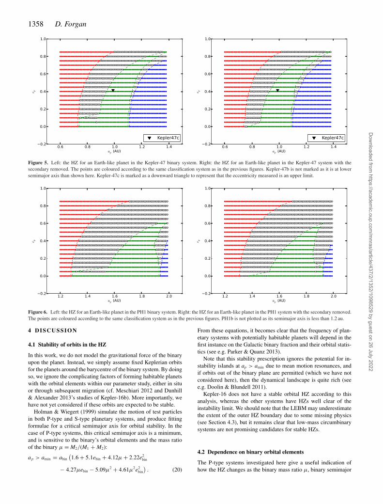
This binary system has the distinction of being the first P-type withmultiple planets detected in orbit (Orosz et al. 2012). Consisting ofa G and M star in a tight low-eccentricity orbit, the system has twoplanets orbiting in the binary plane at 49 d (Kepler-47b) and 303 d(Kepler-47c). The outer planet is thought to be in the HZ, althoughwith the eccentricity of the planet established only as an upper limit(ep < 0.411), it is unclear how long it will spend in the spatialHZ, as noted by both Kane & Hinkel (2013) and Haghighipour &Kaltenegger (2013). Fig. 5 shows the orbital HZ constructed for the

Kepler-47 binary system and for the Kepler-47 primary alone. Thepresence of the M star has little effect on the HZ – the increased fluxallows low-eccentricity planets to be more habitable at semimajoraxes between 0.7 and 0.9 au, but otherwise there is little else toreport.

Kepler-47b has a near-circular orbit at 0.2956 au, and isclearly not in the HZ. Despite its currently uncertain eccentricity,Kepler-47c does indeed appear to be warm and habitable, with lowclimate variations. If Kepler-47c possessed an eccentricity largerthan around 0.5, then it would fall into the region of parameterspace occupied by transient classifications. Again, we should reallyonly consider moons of Kepler-47c for Earth-like habitability, asthe planet is Neptune sized (Orosz et al. 2012).

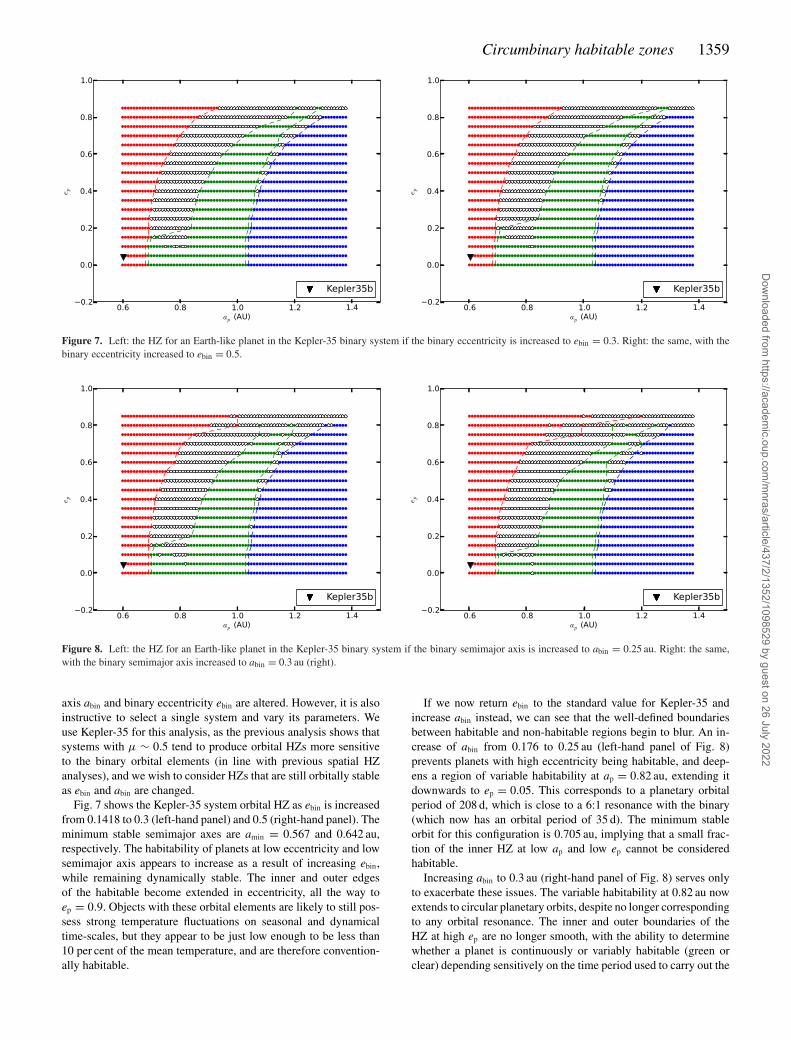
3.5 PH-1

PH-1 (also designated Kepler-64) is a quadruple star system, withthe planet PH1b orbiting an F and M binary system. The othertwo stars in the PH1 system form a separate binary which orbits ata distance of 1000 au, which is sufficiently distant to neglect theirfluxes. The planet was detected by the PlanetHunters citizen scienceprogramme (Schwamb et al. 2013) and orbits with a period of 138 d.This system possesses the most extreme stellar mass ratio, and thisis reflected in Fig. 6, which shows the orbital HZs constructedboth with and without the presence of the M star. The two figuresare close to identical, with the exception of low-eccentricity, low-semimajor-axis planets becoming slightly more habitable when thesecondary is added, thanks to the cooling effect of eclipses. In thesingle-star case (right-hand panel), the inner and outer HZ edgesmeet at ep = 0.6 – with the addition of the second star, the inner andouter edges no longer meet, as the outer edge is pushed to 1.99 au.

The binary orbital period is 20 d (as the eccentricity is not con-strained by observations, we assume that the binary orbit is circular).Hence, as habitable planets will orbit with periods of 500 d or more,the effect of such frequent eclipses on the planetary climate is soft-ened by the atmospheric thermal inertia of the planet. As a 0.5 MJup

planet orbits well within the inner HZ boundary, it is clear that PH1bis not habitable and is unlikely to host habitable moons.

Dow


ic.oup.com/m


1358 D. Forgan

Figure 5. Left: the HZ for an Earth-like planet in the Kepler-47 binary system. Right: the HZ for an Earth-like planet in the Kepler-47 system with thesecondary removed. The points are coloured according to the same classification system as in the previous figures. Kepler-47b is not marked as it is at lowersemimajor axis than shown here. Kepler-47c is marked as a downward triangle to represent that the eccentricity measured is an upper limit.

Figure 6. Left: the HZ for an Earth-like planet in the PH1 binary system. Right: the HZ for an Earth-like planet in the PH1 system with the secondary removed.The points are coloured according to the same classification system as in the previous figures. PH1b is not plotted as its semimajor axis is less than 1.2 au.

4 D ISC U SSION

4.1 Stability of orbits in the HZ

In this work, we do not model the gravitational force of the binaryupon the planet. Instead, we simply assume fixed Keplerian orbitsfor the planets around the barycentre of the binary system. By doingso, we ignore the complicating factors of forming habitable planetswith the orbital elements within our parameter study, either in situor through subsequent migration (cf. Meschiari 2012 and Dunhill& Alexander 2013’s studies of Kepler-16b). More importantly, wehave not yet considered if these orbits are expected to be stable.

Holman & Wiegert (1999) simulate the motion of test particlesin both P-type and S-type planetary systems, and produce fittingformulae for a critical semimajor axis for orbital stability. In thecase of P-type systems, this critical semimajor axis is a minimum,and is sensitive to the binary’s orbital elements and the mass ratioof the binary μ = M2/(M1 + M2):

ap > amin = abin

(1.6 + 5.1ebin + 4.12μ + 2.22e2

bin

− 4.27μebin − 5.09μ2 + 4.61μ2e2bin

). (20)

From these equations, it becomes clear that the frequency of plan-etary systems with potentially habitable planets will depend in thefirst instance on the Galactic binary fraction and their orbital statis-tics (see e.g. Parker & Quanz 2013).

Note that this stability prescription ignores the potential for in-stability islands at ap > amin due to mean motion resonances, andif orbits out of the binary plane are permitted (which we have notconsidered here), then the dynamical landscape is quite rich (seee.g. Doolin & Blundell 2011).

Kepler-16 does not have a stable orbital HZ according to thisanalysis, whereas the other systems have HZs well clear of theinstability limit. We should note that the LEBM may underestimatethe extent of the outer HZ boundary due to some missing physics(see Section 4.3), but it remains clear that low-mass circumbinarysystems are not promising candidates for stable HZs.

4.2 Dependence on binary orbital elements

The P-type systems investigated here give a useful indication ofhow the HZ changes as the binary mass ratio μ, binary semimajor

Dow


ic.oup.com/m



Figure 7. Left: the HZ for an Earth-like planet in the Kepler-35 binary system if the binary eccentricity is increased to ebin = 0.3. Right: the same, with thebinary eccentricity increased to ebin = 0.5.

Figure 8. Left: the HZ for an Earth-like planet in the Kepler-35 binary system if the binary semimajor axis is increased to abin = 0.25 au. Right: the same,with the binary semimajor axis increased to abin = 0.3 au (right).

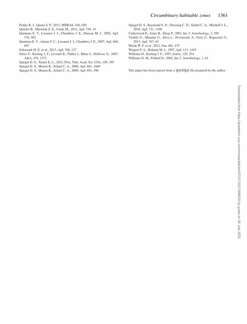
axis abin and binary eccentricity ebin are altered. However, it is alsoinstructive to select a single system and vary its parameters. Weuse Kepler-35 for this analysis, as the previous analysis shows thatsystems with μ ∼ 0.5 tend to produce orbital HZs more sensitiveto the binary orbital elements (in line with previous spatial HZanalyses), and we wish to consider HZs that are still orbitally stableas ebin and abin are changed.

Fig. 7 shows the Kepler-35 system orbital HZ as ebin is increasedfrom 0.1418 to 0.3 (left-hand panel) and 0.5 (right-hand panel). Theminimum stable semimajor axes are amin = 0.567 and 0.642 au,respectively. The habitability of planets at low eccentricity and lowsemimajor axis appears to increase as a result of increasing ebin,while remaining dynamically stable. The inner and outer edgesof the habitable become extended in eccentricity, all the way toep = 0.9. Objects with these orbital elements are likely to still pos-sess strong temperature fluctuations on seasonal and dynamicaltime-scales, but they appear to be just low enough to be less than10 per cent of the mean temperature, and are therefore convention-ally habitable.

If we now return ebin to the standard value for Kepler-35 andincrease abin instead, we can see that the well-defined boundariesbetween habitable and non-habitable regions begin to blur. An in-crease of abin from 0.176 to 0.25 au (left-hand panel of Fig. 8)prevents planets with high eccentricity being habitable, and deep-ens a region of variable habitability at ap = 0.82 au, extending itdownwards to ep = 0.05. This corresponds to a planetary orbitalperiod of 208 d, which is close to a 6:1 resonance with the binary(which now has an orbital period of 35 d). The minimum stableorbit for this configuration is 0.705 au, implying that a small frac-tion of the inner HZ at low ap and low ep cannot be consideredhabitable.

Increasing abin to 0.3 au (right-hand panel of Fig. 8) serves onlyto exacerbate these issues. The variable habitability at 0.82 au nowextends to circular planetary orbits, despite no longer correspondingto any orbital resonance. The inner and outer boundaries of theHZ at high ep are no longer smooth, with the ability to determinewhether a planet is continuously or variably habitable (green orclear) depending sensitively on the time period used to carry out the

Dow


ic.oup.com/m


1360 D. Forgan

averaging. The minimum stable orbit moves to 0.845 au, renderingmost of the inner HZ dynamically unstable.

4.3 Limitations of the model

Using an LEBM by definition requires some concessions to sim-plicity, especially if the goal is to run a large number of simulations.However, we acknowledge that there are some potential improve-ments that should be considered in future work.

As previously mentioned, the orbits of the planets are fixed andKeplerian. A more accurate representation would involve specifyinga Keplerian orbit as initial conditions and allowing the orbit toevolve under the gravitational influence of both stars in the system,either via full N-body calculations (e.g. Meschiari 2012) or usinganalytic expressions which assume the planet mass to be negligible(e.g. Leung & Lee 2013). The non-Keplerian orbits that result fromthese calculations will add important variations in climate, whichmay make planets previously classified as ‘habitable’ into ‘transient’planets (especially the low-semimajor-axis, low-eccentricity planetsthat are commonly classified as habitable), or set up long-termMilankovitch cycles (Spiegel et al. 2010).

Also, the precession of periastron in circumbinary systems willstrongly affect the range of seasonal variations eccentric planetswill experience, as the longitude of solstices shifts further fromthe longitude of periastron (Doolin & Blundell 2011; Armstronget al. 2013). Kepler-34b is expected to undergo a complete cycleof periapse precession in around 20 000 yr, whereas Kepler-35b isexpected to do so in less than 10 000 yr (Welsh et al. 2012). Thesetime-scales are similar to the aforementioned Milankovitch cyclesmeasured on Earth.

When comparing this paper to analytical calculations of the spa-tial HZ, we find that our calculation of the outer HZ boundary (atzero eccentricity) is typically lower than that of the other authors.This is most likely due to the rapid snowball albedo effect presentdue to the freezing of ice, which does not have a counter-opposingmechanism to suppress it (excluding adding more radiation to meltthe ice). In reality, more accurate modelling of the carbon–silicatecycle (Williams & Kasting 1997) would allow cooler planets tomodify their atmospheric CO2 levels. As such, we do not fullymodel the ‘maximum greenhouse’ conditions that are a standard ofspatial HZ calculations, and this is an important feature that mustbe added to future models.

5 C O N C L U S I O N S

We have used one-dimensional LEBM to investigate the HZs ofplanets orbiting P-type star systems. By running many models foreach star system, an ‘orbital HZ’ can be produced, which maps outthe HZ in terms of the planet’s orbital elements. This numericalanalysis is complementary to the common practice of mapping outthe HZ in terms of its spatial extent using analytical calculations.With the use of LEBMs, the orbital HZ allows the effects of stellareclipses and planet eccentricity to be more simply incorporated.

We apply this technique to the circumbinary planetary systemsKepler-16, Kepler-34, Kepler-35, Kepler-47 and PH1. In general,our orbital HZs are consistent with the spatial HZs derived by otherauthors (e.g. Haghighipour & Kaltenegger 2013; Kane & Hinkel2013). As has been found previously, the HZ strongly deviates fromthe single-star HZ when the stars are of approximately equal mass.If the primary is much more massive than the secondary, then thesingle-star HZ and circumbinary HZs are very similar, although wenote that in the case of Kepler-16, which contains two low-mass

stars with a relatively large mass difference, eclipses can becomeimportant.

Of the circumbinary planets orbiting the binaries, we investigatedthat Kepler-47c was the only planet found to reside within the HZ.We are able to make this determination despite the uncertainty ofthe planet’s eccentricity, an advantage of orbital HZ modelling.Kepler-47c is therefore an interesting target for future exomoondetections, as while Kepler-47c is not Earth-like, it may possessterrestrial moons. Kepler-34b would be marginally habitable if itwere of Earth mass – if it possesses an Earth-like moon, it may beable to sustain a biosphere, but it would need to be robust againststrong oscillations in the moon’s climate.

While we have not explicitly simulated the orbital stability ofthese planets, previous analytical calculations of the minimum semi-major axis for a stable circumbinary orbit indicate that with theexception of Kepler-16b, the HZs produced in this work shouldbe amenable to terrestrial planets on stable orbits. However, thedynamical complexity of circumbinary systems warrants furtherinvestigation with more appropriate gravitational physics included.

AC K N OW L E D G E M E N T S

DF gratefully acknowledges support from STFC grantST/J001422/1. The author would like to thank the referees for theirinvaluable comments which greatly improved this paper.

R E F E R E N C E S

Abe Y., Abe-Ouchi A., Sleep N. H., Zahnle K. J., 2011, Astrobiology, 11,443

Anglada-Escude G. et al., 2013, A&A, 556, A126Armstrong D. et al., 2013, MNRAS, 434, 3047Borucki W. J. et al., 2012, ApJ, 745, 120Borucki W. J. et al., 2013, Sci, 340, 587Del Genio A., 1993, Icarus, 101, 1Del Genio A., 1996, Icarus, 120, 332Doolin S., Blundell K. M., 2011, MNRAS, 418, 2656Doyle L. R. et al., 2011, Sci, 333, 1602Dressing C. D., Spiegel D. S., Scharf C. A., Menou K., Raymond S. N.,

2010, ApJ, 721, 1295Dunhill A., Alexander R., 2013, MNRAS, 435, 2328Eggl S., Pilat-Lohinger E., Georgakarakos N., Gyergyovits M., Funk B.,

2012, ApJ, 752, 74Farrell B. F., 1990, J. Atmos. Sci., 47, 2986Forgan D., 2012, MNRAS, 422, 1241Forgan D., Kipping D., 2013, MNRAS, 432, 2994Haghighipour N., Kaltenegger L., 2013, ApJ, 777, 166Hart M. H., 1979, Icarus, 37, 351Heller R., 2012, A&A, 545, L8Holman M. J., Wiegert P. A., 1999, ApJ, 117, 621Huang S.-S., 1959, PASP, 71, 421Kaltenegger L., Haghighipour N., 2013, ApJ, 777, 165Kaltenegger L., Sasselov D., 2011, ApJ, 736, L25Kane S. R., Gelino D. M., 2012a, Astrobiology, 12, 940Kane S. R., Gelino D. M., 2012b, PASP, 124, 323Kane S. R., Hinkel N. R., 2013, ApJ, 762, 7Kasting J., Whitmire D., Reynolds R., 1993, Icarus, 101, 108Kipping D. M., Forgan D., Hartman J., Nesvorny D., Bakos G. A., Schmitt

A. R., Buchhave L. A., 2013, ApJ, 777, 134Kopparapu R. K. et al., 2013, ApJ, 765, 131Leung G. C. K., Lee M. H., 2013, ApJ, 763, 107Mayor M., Queloz D., 1995, Nat, 378, 355Meschiari S., 2012, ApJ, 752, 71North G., Cahalan R., Coakley J., 1981, Rev. Geophys. Space Phys., 19, 91Orosz J. A. et al., 2012, Sci, 337, 1511

Dow


ic.oup.com/m



Parker R. J., Quanz S. P., 2013, MNRAS, 436, 650Quarles B., Musielak Z. E., Cuntz M., 2012, ApJ, 750, 14Quintana E. V., Lissauer J. J., Chambers J. E., Duncan M. J., 2002, ApJ,

576, 982Quintana E. V., Adams F. C., Lissauer J. J., Chambers J. E., 2007, ApJ, 660,

807Schwamb M. E. et al., 2013, ApJ, 768, 127Selsis F., Kasting J. F., Levrard B., Paillet J., Ribas I., Delfosse X., 2007,

A&A, 476, 1373Spiegel D. S., Turner E. L., 2012, Proc. Natl. Acad. Sci. USA, 109, 395Spiegel D. S., Menou K., Scharf C. A., 2008, ApJ, 681, 1609Spiegel D. S., Menou K., Scharf C. A., 2009, ApJ, 691, 596

Spiegel D. S., Raymond S. N., Dressing C. D., Scharf C. A., Mitchell J. L.,2010, ApJ, 721, 1308

Underwood D., Jones B., Sleep P., 2003, Int. J. Astrobiology, 2, 289Vladilo G., Murante G., Silva L., Provenzale A., Ferri G., Ragazzini G.,

2013, ApJ, 767, 65Welsh W. F. et al., 2012, Nat, 481, 475Wiegert P. A., Holman M. J., 1997, ApJ, 113, 1445Williams D., Kasting J. F., 1997, Icarus, 129, 254Williams D. M., Pollard D., 2002, Int. J. Astrobiology, 1, 61

This paper has been typeset from a TEX/LATEX file prepared by the author.

Dow


ic.oup.com/m


assessing circumbinary habitable zones using latitudinal

Documents