J. Stat. M

ech. (2014) P09036

ournal of Statistical Mechanics:J Theory and Experiment

Large lattice fractional Fokker–Planckequation

Vasily E TarasovSkobeltsyn Institute of Nuclear Physics, Lomonosov Moscow State University,Moscow 119991, RussiaE-mail: tarasov@theory.sinp.msu.ru

Received 2 June 2014Accepted for publication 4 August 2014Published 30 September 2014

Online at stacks.iop.org/JSTAT/2014/P09036doi:10.1088/1742-5468/2014/09/P09036

Abstract. An equation of long-range particle drift and diffusion on a 3D physicallattice is suggested. This equation can be considered as a lattice analog of thespace-fractional Fokker–Planck equation for continuum. The lattice approachgives a possible microstructural basis for anomalous diffusion in media thatare characterized by the non-locality of power law type. In continuum limitthe suggested 3D lattice Fokker–Planck equations give fractional Fokker–Planckequations for continuous media with power law non-locality that is describedby derivatives of non-integer orders. The consistent derivation of the fractionalFokker–Planck equation is proposed as a new basis to describe space-fractionaldiffusion processes.

Keywords: diffusion

c© 2014 IOP Publishing Ltd and SISSA Medialab srl 1742-5468/14/P09036+23$33.00

J. Stat. M

ech. (2014) P09036

Large lattice fractional Fokker–Planck equation

Contents

1. Introduction 2

2. Lattice with long-range drift and diffusion 4

3. Continuum limit for lattice equations 123.1. Continuum limit for lattice probability density . . . . . . . . . . . . . . . . . . . . . . . . . . . . . . 123.2. Continuum limit of lattice operators . . . . . . . . . . . . . . . . . . . . . . . . . . . . . . . . . . . . . . . . 13

4. Fractional Fokker–Planck equation for continuum 16

5. Conclusion 19

Appendix A. Riesz fractional integral 20

References 20

1. Introduction

Fokker–Planck equations are usually used to describe the Brownian motion of particles [1].These equations describe the change of probability of a random function in space and timein diffusion processes. The Fokker–Planck equation is usually the second-order partialdifferential equation of parabolic type. In many studies of diffusion processes in complexmedia, the usual second-order Fokker–Planck equation may not be adequate. In particular,the probability density may have a thicker tail than the Gaussian probability density andcorrespondent correlation functions may decay to zero much slower than the functions forusual diffusion processes resulting in long-range dependence. This phenomenon is knownas anomalous diffusion [2–4]. Anomalous diffusion processes can be characterized by apower law mean squared displacement of the form [2–4]

〈x2(t)〉 =2 K(α)tα

Γ(α + 1), (1)

where Γ(z) is the gamma function, α is the anomalous diffusion exponent and K(α)is the anomalous diffusion constant. In equation (1), we use the second moment thatis defined in terms of the ensemble average. Depending on the value of α, we usuallydistinguish sub-diffusion for 0 < α < 1 or super-diffusion for α > 1. There are two limitcases such as the normal diffusion (α = 1) and the ballistic motion (α = 2). One possibleapproach to describe the anomalous diffusion is based on the continuous time random walkmodels [5] in which the particles are considered as random walkers with step lengths r andwaiting times t. An important role is played by the anomalous diffusion processes with thePoissonian waiting time and the Levy distribution for the jump length. The Levy flights [2]are random walks in which the step lengths (long jumps) have a probability distributionthat is heavy-tailed. The Levy motion can be described by a generalized diffusion equation

doi:10.1088/1742-5468/2014/09/P09036 2

J. Stat. M

ech. (2014) P09036

Large lattice fractional Fokker–Planck equation

with space derivatives of non-integer orders μ, [4]. The fractional moment of order δ forLevy flights has the form 〈|x(t)|δ〉 ∼ tδ/μ, where 0 < δ < μ � 2.

Derivatives of non-integer orders [6–13] play an important role in describing particletransport in anomalous diffusion [4, 14–19] and have a wide application in various areasof physics (see, for example, [20–28]). Various approaches lead to different types of space–time fractional Fokker–Planck equations. Usually the space-fractional Fokker–Planckequations are obtained from the second-order differential equations by replacing the first-order and second-order space derivatives by fractional-order derivatives [7]. FractionalFokker–Planck equations with coordinate derivatives of non-integer order have beensuggested in [29]. The solutions and properties of these equations are described in [15,30].The Fokker–Planck equation with fractional coordinate derivatives was also considered in[14, 31–35]. It should be noted that the fractional Fokker–Planck equations can be derivedfrom the probabilistic continuous time random walk [36–38]. In this paper we propose aconsistent derivation of the space-fractional Fokker–Planck equation based on a latticemodel with long-range drift and diffusion that is considered as a microstructural basis todescribe fractional diffusion processes in continua.

A discrete lattice version of the Fokker–Planck equation in analogy with the latticeBoltzmann models has been suggested in [40–42]. These models are used to solve theequations of hydrodynamics and cavity flow simulations [43]. The lattice Fokker–Planckequation is applied to the study of electro-rheological transport of 1D charged fluid [44] andit is used in phase-space descriptions of inertial polymer dynamics [45]. All these latticeFokker–Planck equations are based on the lattice Boltzmann discretization approach.

In this paper, we propose a lattice equation for probability density of particlein unbounded homogeneous 3D lattice with long-range drift and diffusion to n-sitefrom all other m-sites (m �= n). We prove that continuous limit for the suggestedlattice Fokker–Planck equation gives the space-fractional Fokker–Planck equation for non-local continuum. The fractional differential equation for continuum contains generalizedconjugate Riesz derivatives of non-integer orders.

Continuum mechanics [46] can be considered as a continuous limit of lattice dynamics[47–50], where the length-scales of a continuum element are much larger than the distancesbetween the lattice particles. The first self-consistent derivation of the Fokker–Planckequation based on the microscopic dynamics for classical and quantum systems wasobtained by Bogolyubov and Krylov [51, 52]. Long-range interactions are important fordifferent problems in statistical mechanics [53–55], kinetic theory and nonequilibriumstatistical mechanics [56,57], theory of non-equilibrium phase transitions [58,59]. As it wasshown in [60, 61] (see also [62–64] and [65–70]), the continuum equations with fractionalderivatives can be directly connected to lattice models with long-range properties. Aconnection between the dynamics of a lattice system of particles with long-range propertiesand the fractional continuum equations are proved by using the transform operation[60, 61]. The papers [60, 61] deal with the 1D lattice models and the correspondent 1Dcontinuum equations. In this paper, we suggest 3D lattice models for space-fractionaldiffusion processes. We propose a general form of 3D lattice Fokker–Planck equation,which leads to a continuum fractional Fokker–Planck equation with space derivativesof non-integer orders by continuous limit. The suggested approach to derive the spacefractional Fokker–Planck equations can serve as a microstructural basis to describe thespatial-fractional diffusion processes.

doi:10.1088/1742-5468/2014/09/P09036 3

J. Stat. M

ech. (2014) P09036

Large lattice fractional Fokker–Planck equation

2. Lattice with long-range drift and diffusion

The lattice is characterized by space periodicity. In an unbounded lattice we can definethree non-coplanar vectors a1, a2, a3, that are the shortest vectors by which a lattice canbe displaced and be brought back into itself. All space lattice sites can be defined by thevector n = (n1, n2, n3), where ni are integer. For simplification, we consider a lattice withmutually perpendicular primitive lattice vectors a1, a2, a3. We choose directions of theaxes of the Cartesian coordinate system to coincide with the vector ai. Then ai = ai ei,where ai = |ai| and ei are the basis vectors of the Cartesian coordinate system. Thissimplification means that the lattice is a primitive orthorhombic Bravais lattice withlong-range drift and diffusion of particles.

If we choose the coordinate origin at one of the sites, then the position vector of anarbitrary lattice site with n = (n1, n2, n3) is written r(n) = n1a1 + n2a2 + n3a3. Thelattice sites are numbered by n, so that the vector n can be considered as a numbervector of the corresponding particle. We assume that the positions of particles coincidewith the lattice sites r(n). The probability density for the lattice site will be denotedby f(n, t) = f(n1, n2, n3, t), where the site is defined by the vector n = (n1, n2, n3). Thefunction f(n, t) satisfies the conditions

+∞∑n1=−∞

+∞∑n2=−∞

+∞∑n3=−∞

f(n1, n2, n3, t) = 1, f(n1, n2, n3, t) � 0 (2)

for all t ∈ R.The equation for probability density of particle in unbounded homogeneous lattice is

∂f(n, t)∂t

= −3∑

i=1

∑mi �=ni

giKiαi

(n − m)f(m, t) +3∑

i,j=1

∑mi �=ni

∑mj �=nj

gijKijαi,βj

(n − m)f(m, t), (3)

where f(n, t) is the probability density function to find the test particle at site n at timet. The italics i, j ∈ {1; 2; 3} are the coordinate indices, gi and gij are lattice couplingconstants. The coefficients Ki

αi(n − m) and Kij

αi,βj(n − m) describe the particle drift and

diffusion on the lattice and it can be called the drift and diffusion kernels for lattice steplength n − m. These kernels describe the long-range drift and diffusion to n-site from allother m-sites. The parameters αi and βj in the kernels are positive real numbers thatcharacterize how quickly the intensity of the drift and diffusion processes in the latticedecrease with increasing the value n − m. These parameters also can be considered asdegrees of the power law of lattice spatial dispersion [65, 68] that is described by non-integer power of the wave vector components.

Equation (3) describes fractional diffusion processes on the physical lattices, wherelong-range jumps can be realized. The Levy motion (flights) for these lattices can bedescribed by the lattice Fokker–Planck equation (3), which is considered as a latticeanalog of the fractional diffusion processes with the Poissonian waiting time and the Levydistribution for the jump length [4].

For simplification, we consider the kernels in the form

Kiαi

(n − m) = Kαi(ni − mi), Kij

αi,βj(n − m) = Kαi

(ni − mi) Kβj(nj − mj), (4)

doi:10.1088/1742-5468/2014/09/P09036 4

J. Stat. M

ech. (2014) P09036

Large lattice fractional Fokker–Planck equation

where i, j = 1, 2, 3. The kernels Kαi(ni −mi), where i = 1, 2, 3, describe long-range jumps

in the direction ai with lattice step length ni −mi in the lattice. The correspondent termswith kernels Kαi

(ni − mi) can be considered as lattice analogs of fractional derivatives oforder αi with respect to coordinate xi = (r, ai). We will consider even and odd types ofthe kernels Kαi

(ni−mi), i = 1, 2, 3, that will be denoted by K+αi

(ni−mi) and K−αi

(ni−mi)respectively.

We assume that the kernels K±α (n) satisfy the following conditions:

(a) The kernels K±α (n) are real-valued functions of integer variable n ∈ Z. The kernels

K+α (n) and K−

α (n) are even and odd functions such that

K+α (−n) = +K+

α (n), K−α (−n) = −K−

α (n) (5)

hold for all n ∈ Z.

(b) The kernels K±α (n) belong to the Hilbert space of square-summable sequences,

∞∑n=1

|K±α (n)|2 < ∞. (6)

(c) The Fourier series transforms K±α (k) of the kernels K±

α (n) in the form

K+α (k) =

+∞∑n=−∞n�=0

e−iknK+α (n) = 2

∞∑n=1

K+α (n) cos(kn), (7)

K−α (k) =

+∞∑n=−∞

e−iknK−α (n) = −2 i

∞∑n=1

K−α (n) sin(kn) (8)

satisfying the conditions

K+α (k) = |k|α + o(|k|α), (k → 0), (9)

and

K−α (k) = i sgn(k) |k|α + o(|k|α), (k → 0) (10)

respectively. Here the little-o notation o(|k|α) means the terms that include higherpowers of |k| than |k|α. The suggested forms (9) and (10) of the Fourier seriestransforms of the kernels K±

α (n) mean that we consider lattices with weak spatialdispersion [65]. The conditions (9) and (10) allow us to consider a wide class of kernelsto describe the long-range lattice drift and diffusion.

In general, the type of dependence of the function K±α (k) on the wave vector k is defined

by the type of spatial dispersion in the lattice [65,68]. For a wide class of processes in thelattice, the wavelength λ holds the relation a0/λ ∼ ka0 1, where a0 is the characteristicsize of the lattice distance such that a0 = max{|a1|, |a2|, |a3|}. In the case ka0 1, where

doi:10.1088/1742-5468/2014/09/P09036 5

J. Stat. M

ech. (2014) P09036

Large lattice fractional Fokker–Planck equation

a0, the spatial dispersion of the lattice is weak. To describe lattices with such propertyit is enough to know the dependence of the function K±

α (k) only for small values k andwe can replace this function by Taylor’s polynomial series. The weak spatial dispersionof the lattices with a power law type of spatial dispersion cannot be described by theusual Taylor approximation. In this case, we should use a fractional Taylor series [65,68].The fractional Taylor series is more adequate for approximation of non-integer power lawfunctions. For example, the usual Taylor series for the power law function K+

α (k) = aα kα

has the infinite by many terms for non-integer α. The fractional Taylor series of order αhas a finite number of terms for this function and the fractional Taylor’s approximationis exact. We can use the fractional Taylor’s series in the Riemann–Liouville form (seechapter 1 section 2.6 [6]) that can be represented as

K+α (kj) = bj(α) |kj|α + o(|kj|α), (11)

where

bj(α) =( RL

0 Dαkj

K+α )(0)

Γ(α + 1), (12)

and C0 Dα

k is the Riemann–Liouville fractional derivative [7] of order 0 < α < 1 withrespect to k. This derivative is defined by

( RL0 Dα

k K+α )(k) =

(ddk

)n (0I

n−αk K+

α

)(k), (13)

where 0Iαk is the left-sided Riemann–Liouville fractional integral of order α > 0 with

respect to k of the form

( 0Iαk K+

α )(k) =1

Γ(α)

∫ k

0

K+α (k′) dk′

(k − k′)1−α, (k > 0). (14)

Using the approximation (11), we neglect a frequency dispersion for simplification, i.e.the parameters bj(α) do not depend on the frequency ω. In suggested lattice models, wedefine the kernels such that the constants gi and gij include the factor bj(α) and as aresult the conditions (9) and (10) hold.

For simplification, we can consider the lattice kernels that are defined by the explicitexpressions in the form

K+α (k) = |k|α, K−

α (k) = i sgn(k) |k|α. (15)

In this case, the inverse relations to the definitions of K±α (k) by equations (7) and (8)

have the forms

K+α (n) =

1π

∫ π

0kα cos(n k) dk, K−

α (n) = − 1π

∫ π

0kα sin(n k) dk. (16)

For non-integer real values of the parameter α, the expressions for the kernels K±α (n−m)

are

K+α (n − m) =

πα

α + 1 1F2

(α + 1

2;12,α + 3

2; −π2 (n − m)2

4

), α > −1, (17)

doi:10.1088/1742-5468/2014/09/P09036 6

J. Stat. M

ech. (2014) P09036

Large lattice fractional Fokker–Planck equation

02

46

X0

2

4

6

Y

-100

0

100

Z

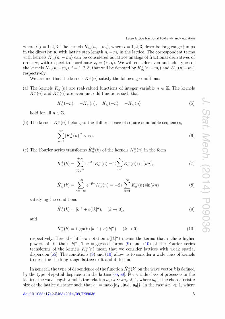
Figure 1. Plot of the function F+(x, y) (19) for the range x ∈ [0, 6] andy = α ∈ [0, 6].

K−α (n − m) = −πα+1 (n − m)

α + 2 1F2

(α + 2

2;32,α + 4

2; −π2 (n − m)2

4

), α > −2, (18)

where 1F2 is the Gauss hypergeometric function (see Chapter 2 in [72]). Note thatexpressions can be used not only for α > 0, but also for some negative values of α.

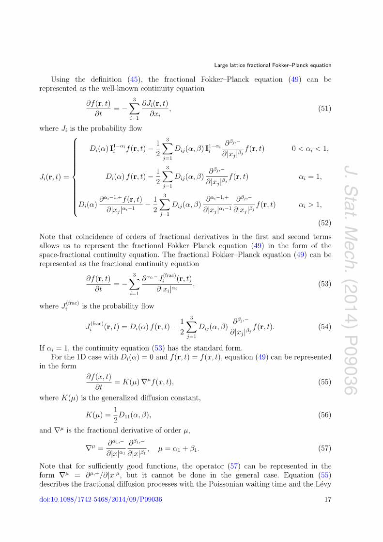
To visualize the properties of the kernels (17) and (18), we give the plots of thefunctions

F+(x, y) =πy

y + 1 1F2

(y + 1

2;12,y + 3

2; −π2 x2

4

), (19)

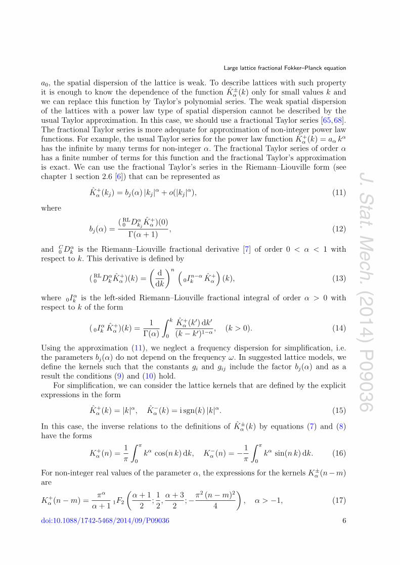
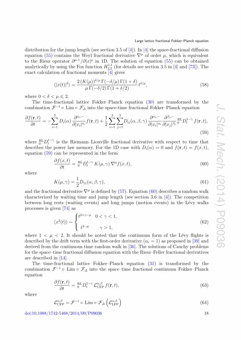
F−(x, y) = −πy+1 x

y + 2 1F2

(y + 2

2;32,y + 4

2; −π2 x2

4

), (20)

where

K±α (n − m) = F±(n − m, α). (21)

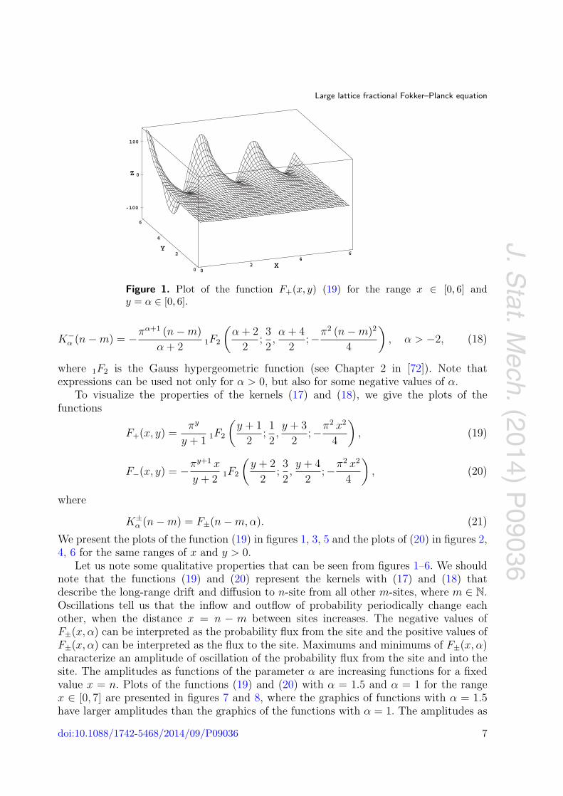
We present the plots of the function (19) in figures 1, 3, 5 and the plots of (20) in figures 2,4, 6 for the same ranges of x and y > 0.

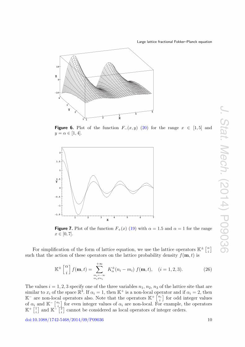
Let us note some qualitative properties that can be seen from figures 1–6. We shouldnote that the functions (19) and (20) represent the kernels with (17) and (18) thatdescribe the long-range drift and diffusion to n-site from all other m-sites, where m ∈ N.Oscillations tell us that the inflow and outflow of probability periodically change eachother, when the distance x = n − m between sites increases. The negative values ofF±(x, α) can be interpreted as the probability flux from the site and the positive values ofF±(x, α) can be interpreted as the flux to the site. Maximums and minimums of F±(x, α)characterize an amplitude of oscillation of the probability flux from the site and into thesite. The amplitudes as functions of the parameter α are increasing functions for a fixedvalue x = n. Plots of the functions (19) and (20) with α = 1.5 and α = 1 for the rangex ∈ [0, 7] are presented in figures 7 and 8, where the graphics of functions with α = 1.5have larger amplitudes than the graphics of the functions with α = 1. The amplitudes as

doi:10.1088/1742-5468/2014/09/P09036 7

J. Stat. M

ech. (2014) P09036

Large lattice fractional Fokker–Planck equation

02

46

X0

2

4

6

Y

-100

0

100

Z

Figure 2. Plot of the function F−(x, y) (20) for the range x ∈ [0, 6] andy = α ∈ [0, 6].

68

1012

14

X0

2

4

6

Y

-40

-20

0

20

40

Z

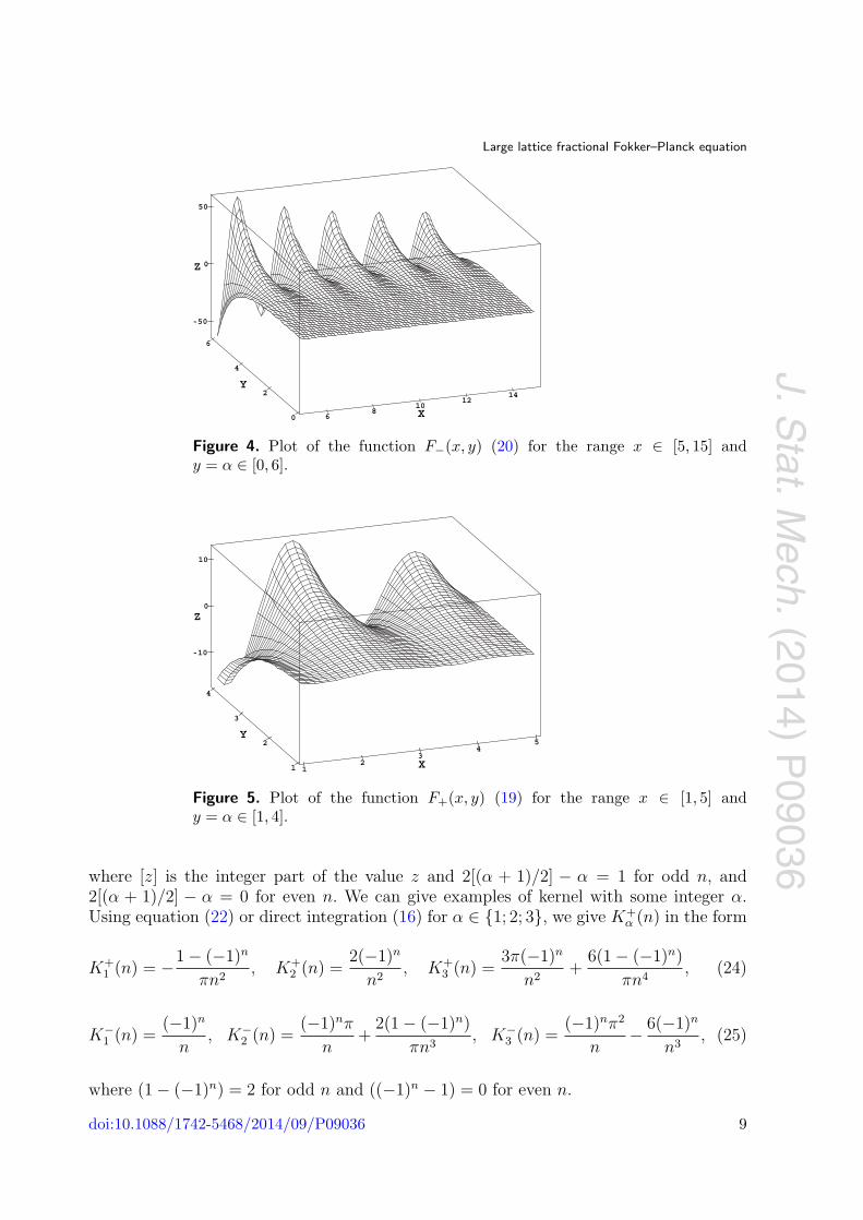
Figure 3. Plot of the function F+(x, y) (19) for the range x ∈ [5, 15] andy = α ∈ [0, 6].

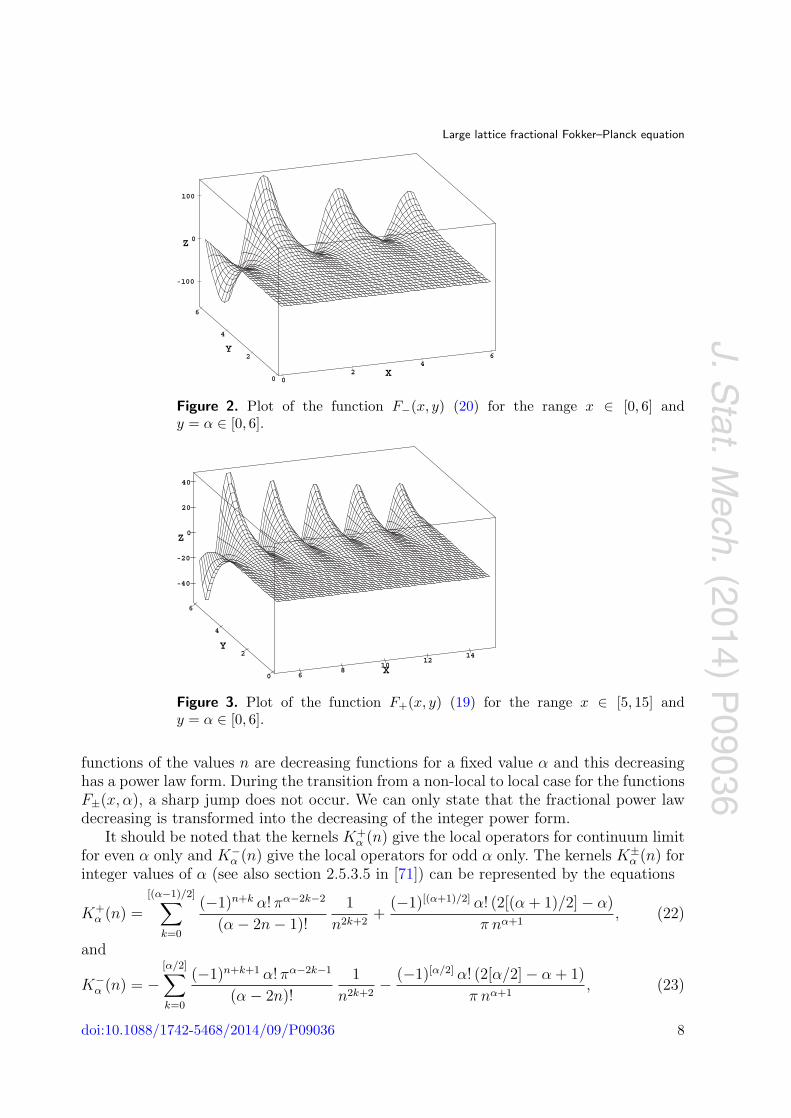
functions of the values n are decreasing functions for a fixed value α and this decreasinghas a power law form. During the transition from a non-local to local case for the functionsF±(x, α), a sharp jump does not occur. We can only state that the fractional power lawdecreasing is transformed into the decreasing of the integer power form.

It should be noted that the kernels K+α (n) give the local operators for continuum limit

for even α only and K−α (n) give the local operators for odd α only. The kernels K±

α (n) forinteger values of α (see also section 2.5.3.5 in [71]) can be represented by the equations

K+α (n) =

[(α−1)/2]∑k=0

(−1)n+k α! πα−2k−2

(α − 2n − 1)!1

n2k+2 +(−1)[(α+1)/2] α! (2[(α + 1)/2] − α)

π nα+1 , (22)

and

K−α (n) = −

[α/2]∑k=0

(−1)n+k+1 α! πα−2k−1

(α − 2n)!1

n2k+2 − (−1)[α/2] α! (2[α/2] − α + 1)π nα+1 , (23)

doi:10.1088/1742-5468/2014/09/P09036 8

J. Stat. M

ech. (2014) P09036

Large lattice fractional Fokker–Planck equation

68

1012

14

X0

2

4

6

Y

-50

0

50

Z

Figure 4. Plot of the function F−(x, y) (20) for the range x ∈ [5, 15] andy = α ∈ [0, 6].

12

34

5

X1

2

3

4

Y

-10

0

10

Z

Figure 5. Plot of the function F+(x, y) (19) for the range x ∈ [1, 5] andy = α ∈ [1, 4].

where [z] is the integer part of the value z and 2[(α + 1)/2] − α = 1 for odd n, and2[(α + 1)/2] − α = 0 for even n. We can give examples of kernel with some integer α.Using equation (22) or direct integration (16) for α ∈ {1; 2; 3}, we give K+

α (n) in the form

K+1 (n) = −1 − (−1)n

πn2 , K+2 (n) =

2(−1)n

n2 , K+3 (n) =

3π(−1)n

n2 +6(1 − (−1)n)

πn4 , (24)

K−1 (n) =

(−1)n

n, K−

2 (n) =(−1)nπ

n+

2(1 − (−1)n)πn3 , K−

3 (n) =(−1)nπ2

n− 6(−1)n

n3 , (25)

where (1 − (−1)n) = 2 for odd n and ((−1)n − 1) = 0 for even n.

doi:10.1088/1742-5468/2014/09/P09036 9

J. Stat. M

ech. (2014) P09036

Large lattice fractional Fokker–Planck equation

12

34

5

X1

2

3

4

Y

-10

0

10

Z

Figure 6. Plot of the function F−(x, y) (20) for the range x ∈ [1, 5] andy = α ∈ [1, 4].

-1.5

-1

-0.5

0

0.5

1

1.5

2

Y

1 2 3 4 5 6 7X

Figure 7. Plot of the function F+(x) (19) with α = 1.5 and α = 1 for the rangex ∈ [0, 7].

For simplification of the form of lattice equation, we use the lattice operators K± [α

i

]such that the action of these operators on the lattice probability density f(m, t) is

K±[α

i

]f(m, t) =

+∞∑mi=−∞mi �=ni

K±α (ni − mi) f(m, t), (i = 1, 2, 3). (26)

The values i = 1, 2, 3 specify one of the three variables n1, n2, n3 of the lattice site that aresimilar to xi of the space R

3. If αi = 1, then K+ is a non-local operator and if αi = 2, then

K− are non-local operators also. Note that the operators K

+[

αi

i

]for odd integer values

of αi and K− [αi

i

]for even integer values of αi are non-local. For example, the operators

K+[1

i

]and K

− [2i

]cannot be considered as local operators of integer orders.

doi:10.1088/1742-5468/2014/09/P09036 10

J. Stat. M

ech. (2014) P09036

Large lattice fractional Fokker–Planck equation

-2

-1

0

1

Y

1 2 3 4 5 6 7X

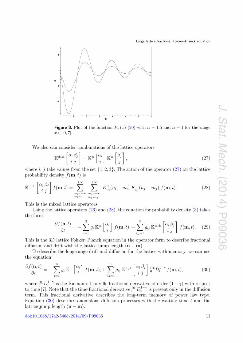
Figure 8. Plot of the function F−(x) (20) with α = 1.5 and α = 1 for the rangex ∈ [0, 7].

We also can consider combinations of the lattice operators

K±,±[αi βj

i j

]= K

±[αi

i

]K

±[βj

j

], (27)

where i, j take values from the set {1; 2; 3}. The action of the operator (27) on the latticeprobability density f(m, t) is

K±,±[αi βj

i j

]f(m, t) =

+∞∑mi=−∞mi �=ni

+∞∑mj=−∞mj �=nj

K±αi

(ni − mi) K±βj

(nj − mj) f(m, t). (28)

This is the mixed lattice operators.Using the lattice operators (26) and (28), the equation for probability density (3) takes

the form

∂f(n, t)∂t

= −3∑

i=1

gi K±[αi

i

]f(m, t), +

3∑i,j=1

gij K±,±[αi βj

i j

]f(m, t). (29)

This is the 3D lattice Fokker–Planck equation in the operator form to describe fractionaldiffusion and drift with the lattice jump length (n − m).

To describe the long-range drift and diffusion for the lattice with memory, we can usethe equation

∂f(n, t)∂t

= −3∑

i=1

gi K±[αi

i

]f(m, t), +

3∑i,j=1

gij K±,±[αi βj

i j

]RL0 D1−γ

t f(m, t), (30)

where RL0 D1−γ

t is the Riemann–Liouville fractional derivative of order (1−γ) with respectto time [7]. Note that the time-fractional derivative RL

0 D1−γt is present only in the diffusion

term. This fractional derivative describes the long-term memory of power law type.Equation (30) describes anomalous diffusion processes with the waiting time t and thelattice jump length (n − m).

doi:10.1088/1742-5468/2014/09/P09036 11

J. Stat. M

ech. (2014) P09036

Large lattice fractional Fokker–Planck equation

We can consider the time-fractional derivatives RL0 D1−γ

t in the first and second terms ofthe right side of the lattice Fokker–Planck equation (29). In this case the time-fractionallattice Fokker–Planck equation has the form

∂f(n, t)∂t

= RL0 D1−γ

t Lα,βLFP f(m, t), (31)

where Lα,βLFP is the lattice Fokker–Planck operator

Lα,βLFP = −

3∑i=1

gi K±[αi

i

]+

3∑i,j=1

gij K±,±[αi βj

i j

]. (32)

Equation (31) describes long-range diffusion and drift with power law memory onorthorhombic Bravais lattices.

3. Continuum limit for lattice equations

3.1. Continuum limit for lattice probability density

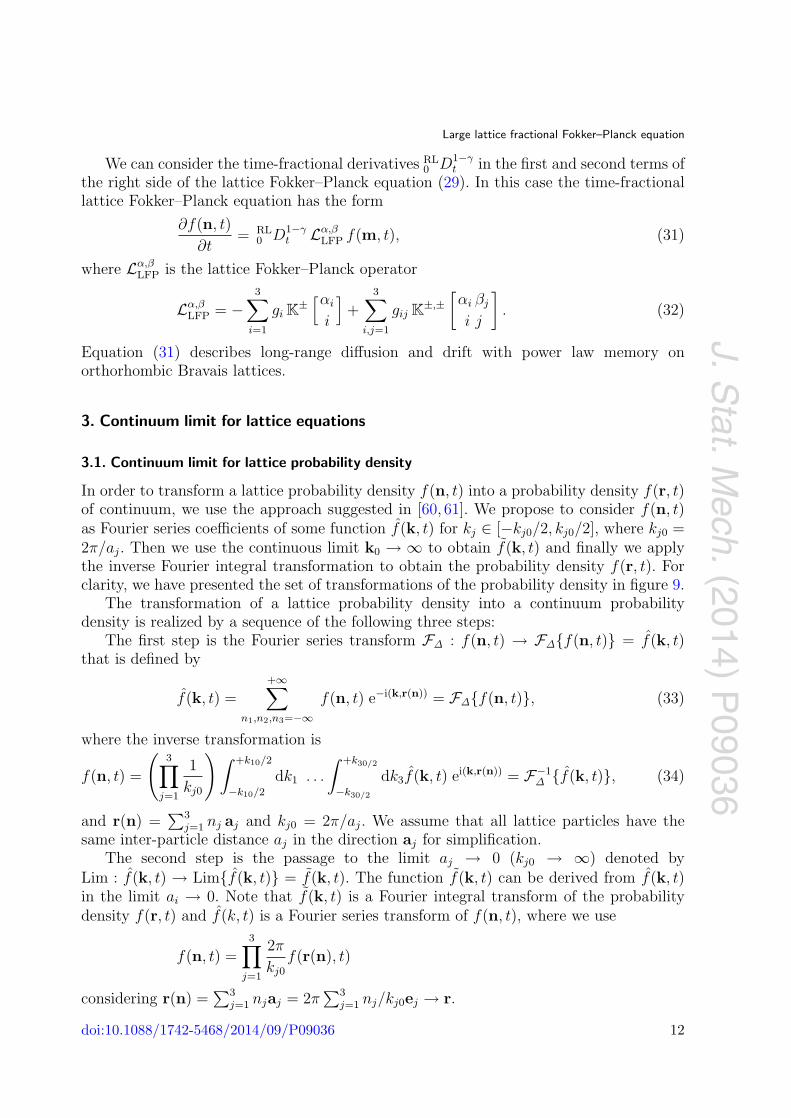
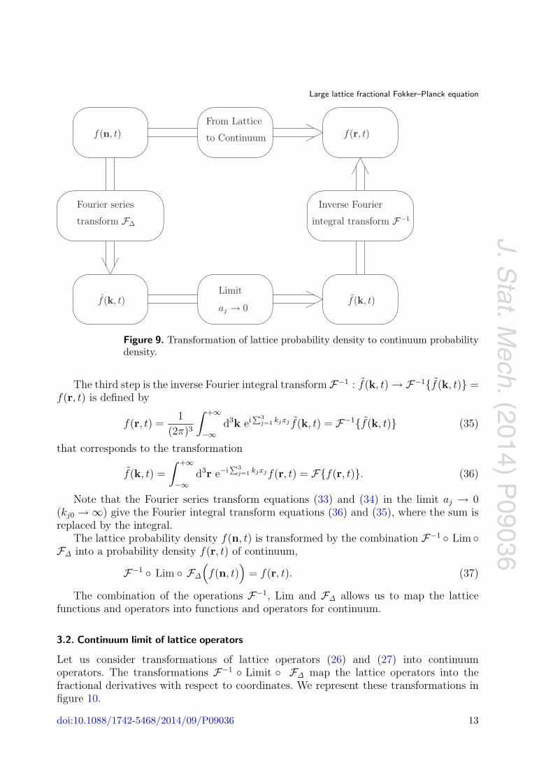
In order to transform a lattice probability density f(n, t) into a probability density f(r, t)of continuum, we use the approach suggested in [60, 61]. We propose to consider f(n, t)as Fourier series coefficients of some function f(k, t) for kj ∈ [−kj0/2, kj0/2], where kj0 =2π/aj. Then we use the continuous limit k0 → ∞ to obtain f(k, t) and finally we applythe inverse Fourier integral transformation to obtain the probability density f(r, t). Forclarity, we have presented the set of transformations of the probability density in figure 9.

The transformation of a lattice probability density into a continuum probabilitydensity is realized by a sequence of the following three steps:

The first step is the Fourier series transform FΔ : f(n, t) → FΔ{f(n, t)} = f(k, t)that is defined by

f(k, t) =+∞∑

n1,n2,n3=−∞f(n, t) e−i(k,r(n)) = FΔ{f(n, t)}, (33)

where the inverse transformation is

f(n, t) =

(3∏

j=1

1kj0

)∫ +k10/2

−k10/2dk1 . . .

∫ +k30/2

−k30/2

dk3f(k, t) ei(k,r(n)) = F−1Δ {f(k, t)}, (34)

and r(n) =∑3

j=1 nj aj and kj0 = 2π/aj. We assume that all lattice particles have thesame inter-particle distance aj in the direction aj for simplification.

The second step is the passage to the limit aj → 0 (kj0 → ∞) denoted byLim : f(k, t) → Lim{f(k, t)} = f(k, t). The function f(k, t) can be derived from f(k, t)in the limit ai → 0. Note that f(k, t) is a Fourier integral transform of the probabilitydensity f(r, t) and f(k, t) is a Fourier series transform of f(n, t), where we use

f(n, t) =3∏

j=1

2πkj0

f(r(n), t)

considering r(n) =∑3

j=1 njaj = 2π∑3

j=1 nj/kj0ej → r.

doi:10.1088/1742-5468/2014/09/P09036 12

J. Stat. M

ech. (2014) P09036

Large lattice fractional Fokker–Planck equation

Figure 9. Transformation of lattice probability density to continuum probabilitydensity.

The third step is the inverse Fourier integral transform F−1 : f(k, t) → F−1{f(k, t)} =f(r, t) is defined by

f(r, t) =1

(2π)3

∫ +∞

−∞d3k ei

∑3j=1 kjxj f(k, t) = F−1{f(k, t)} (35)

that corresponds to the transformation

f(k, t) =∫ +∞

−∞d3r e−i

∑3j=1 kjxjf(r, t) = F{f(r, t)}. (36)

Note that the Fourier series transform equations (33) and (34) in the limit aj → 0(kj0 → ∞) give the Fourier integral transform equations (36) and (35), where the sum isreplaced by the integral.

The lattice probability density f(n, t) is transformed by the combination F−1 ◦ Lim ◦FΔ into a probability density f(r, t) of continuum,

F−1 ◦ Lim ◦ FΔ

(f(n, t)

)= f(r, t). (37)

The combination of the operations F−1, Lim and FΔ allows us to map the latticefunctions and operators into functions and operators for continuum.

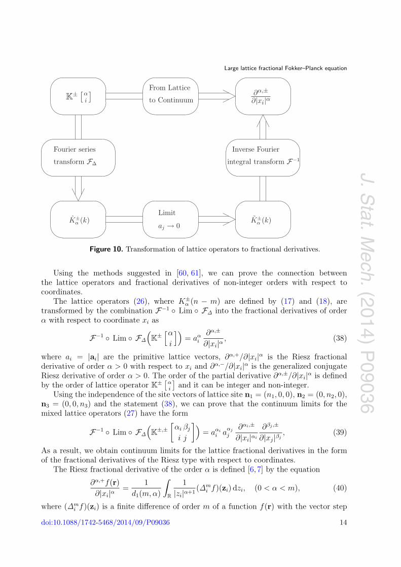
3.2. Continuum limit of lattice operators

Let us consider transformations of lattice operators (26) and (27) into continuumoperators. The transformations F−1 ◦ Limit ◦ FΔ map the lattice operators into thefractional derivatives with respect to coordinates. We represent these transformations infigure 10.

doi:10.1088/1742-5468/2014/09/P09036 13

J. Stat. M

ech. (2014) P09036

Large lattice fractional Fokker–Planck equation

Figure 10. Transformation of lattice operators to fractional derivatives.

Using the methods suggested in [60, 61], we can prove the connection betweenthe lattice operators and fractional derivatives of non-integer orders with respect tocoordinates.

The lattice operators (26), where K±α (n − m) are defined by (17) and (18), are

transformed by the combination F−1 ◦ Lim ◦ FΔ into the fractional derivatives of orderα with respect to coordinate xi as

F−1 ◦ Lim ◦ FΔ

(K

±[α

i

])= aα

i

∂α,±

∂|xi|α , (38)

where ai = |ai| are the primitive lattice vectors, ∂α,+/∂|xi|α is the Riesz fractionalderivative of order α > 0 with respect to xi and ∂α,−/∂|xi|α is the generalized conjugateRiesz derivative of order α > 0. The order of the partial derivative ∂α,±/∂|xi|α is definedby the order of lattice operator K

± [αi

]and it can be integer and non-integer.

Using the independence of the site vectors of lattice site n1 = (n1, 0, 0), n2 = (0, n2, 0),n3 = (0, 0, n3) and the statement (38), we can prove that the continuum limits for themixed lattice operators (27) have the form

F−1 ◦ Lim ◦ FΔ

(K

±,±[αi βj

i j

])= aαi

i aαj

j

∂αi,±

∂|xi|αi

∂βj ,±

∂|xj|βj, (39)

As a result, we obtain continuum limits for the lattice fractional derivatives in the formof the fractional derivatives of the Riesz type with respect to coordinates.

The Riesz fractional derivative of the order α is defined [6, 7] by the equation

∂α,+f(r)∂|xi|α =

1d1(m, α)

∫R

1|zi|α+1 (Δm

i f)(zi) dzi, (0 < α < m), (40)

where (Δmi f)(zi) is a finite difference of order m of a function f(r) with the vector step

doi:10.1088/1742-5468/2014/09/P09036 14

J. Stat. M

ech. (2014) P09036

Large lattice fractional Fokker–Planck equation

zi = xi ei ∈ R3 for the point r ∈ R

3. The non-centered difference is

(Δmi f)(zi) =

m∑k=0

(−1)k m!k! (m − k)!

f(r − k zi), (41)

and the centered difference is

(Δmi f)(zi) =

m∑k=0

(−1)k m!k! (m − k)!

f(r − (m/2 − k) zi). (42)

The constant d1(m, α) is defined by

d1(m, α) =π3/2Am(α)

2αΓ(1 + α/2)Γ((1 + α)/2) sin(πα/2),

where

Am(α) = 2m∑

j=0

(−1)j−1 m!j!(m − j)!

jα

in the case of the non-centered difference (41) and

Am(α) = 2[m/2]∑j=0

(−1)j−1 m!j!(m − j)!

(m/2 − j)α

in the case of the centered difference (42). The constants d1(m, α) is different from zerofor all α > 0 in the case of an even m and centered difference (Δm

i f) (see Theorem 26.1in [6]). In the case of a non-centered difference the constant d1(m, α) vanishes if and onlyif α = 1, 3, 5, . . . , 2[m/2] − 1. Note that the integral (40) does not depend on the choiceof m > α. The Fourier transform F of the Riesz fractional derivative is given by

F(

∂α,+f(r)∂|xi|α

)(k) = |ki|α(Ff)(k). (43)

Equation (43) can be considered as a definition of the Riesz fractional derivative of order α.Using (−i)2j = (−1)j, the Riesz derivatives for even α = 2j are

∂2j,+f(r)∂|xi|2j

= (−1)j ∂2jf(r)∂x2j

i

. (44)

For α = 2 the Riesz derivative looks like the Laplace operator. The fractional derivatives∂α,+/∂|xi|α for even orders α are local operators. Note that the Riesz derivative ∂1,+/∂|xi|1cannot be considered as a derivative of first-order with respect to |xi|. For α = 1 it lookslike ‘the square root of the Laplacian’. The Riesz derivatives for odd orders α = 2j + 1are non-local operators that cannot be considered as usual derivatives ∂2j+1/∂x2j+1

i .We also define the new fractional derivatives ∂α,−/∂|xi|α by the equation

∂α,−

∂|xi|α =

⎧⎪⎪⎪⎪⎪⎪⎪⎨⎪⎪⎪⎪⎪⎪⎪⎩

∂

∂xi

I1−αi 0 < α < 1,

∂

∂xi

α = 1,

∂

∂xi

∂α−1,+

∂|xi|α−1 α > 1,

(45)

doi:10.1088/1742-5468/2014/09/P09036 15

J. Stat. M

ech. (2014) P09036

Large lattice fractional Fokker–Planck equation

where ∂/∂xi is the usual derivative of first-order with respect to coordinate xi and I1−αi

is the Riesz potential of order (1 − α) (see appendix A) with respect to xi,

I1−αi f(r) =

∫R1

R1−α(xi − zi) f(r + (zi − xi)ei)dzi, (0 < α < 1), (46)

where ei is the basis of the Cartesian coordinate system. For 0 < α < 1 the operator∂α,−/∂|xi|α is called the conjugate Riesz derivative [9]. Therefore, the operator ∂α,−/∂|xi|αfor all α > 0 can be called the generalized conjugate Riesz derivative.

The Fourier transform F of the fractional derivative (45) is given by

F(

∂α,−f(r)∂|xi|α

)(k) = i ki |ki|α−1(Ff)(k) = i sgn(ki) |ki|α(Ff)(k). (47)

Using (44) and (45), we get

∂2j+1,−f(r)∂|xi|2j+1 = (−1)j ∂2j+1f(r)

∂x2j+1i

. (48)

The fractional derivatives ∂α,−/∂|xi|α for odd orders α are local operators. Note that thegeneralized conjugate Riesz derivative ∂2,−/∂|xi|2 cannot be considered as a derivative ofsecond-order with respect to |xi|. The derivatives ∂α,−/∂|xi|α for even orders α = 2j arenon-local operators that cannot be considered as usual derivatives ∂2j/∂x2j

i . For α = 2the generalized conjugate Riesz derivative is not the Laplacian.

Equations (44) and (48) allow us to state that the usual local partial derivatives ofinteger orders are obtained from the operators ∂α,±/∂|xi|α in the following two cases: (1)for odd values α = 2j + 1 > 0 by ∂α,−/∂|xi|α only; (2) for even values α = 2j > 0 by∂α,+/∂|xi|α only. The operators ∂α,+/∂|xi|α with integer odd α = 2j + 1 and ∂α,−/∂|xi|αwith integer even α = 2j, where n ∈ N, are non-local operators. Therefore we considerthe lattice equations with the lattice operators K

− [αi

i

]and K

−,−[

αi βj

i j

]as main lattice

models to have the usual equations with local spatial derivatives in the case αi = βi = 1for all i = 1, 2, 3.

4. Fractional Fokker–Planck equation for continuum

Using the statements (37), (38) and (39), where K−α (n−m) are defined by (18), the lattice

Fokker–Planck equation (29) are transformed by the combination F−1 ◦ Lim ◦ FΔ intothe fractional Fokker–Planck equation with derivatives of non-integer orders with respectto space coordinates. This space-fractional Fokker–Planck equation for the probabilitydensity f(r, t) has the form

∂f(r, t)∂t

= −3∑

i=1

Di(α)∂αi,−

∂|xi|αif(r, t) +

12

3∑i=1

3∑j=1

Dij(α, β)∂αi,−

∂|xi|αi

∂βj ,−

∂|xj|βjf(r, t), (49)

where Di(α) is the drift vector and Dij(α, β) is the diffusion tensor for the continuumthat are defined by the lattice coupling constants gi and gij by the relations

Di(α) = aαii gi, Dij(α, β) = 2 aαi

i aβj gij. (50)

doi:10.1088/1742-5468/2014/09/P09036 16

J. Stat. M

ech. (2014) P09036

Large lattice fractional Fokker–Planck equation

Using the definition (45), the fractional Fokker–Planck equation (49) can berepresented as the well-known continuity equation

∂f(r, t)∂t

= −3∑

i=1

∂Ji(r, t)∂xi

, (51)

where Ji is the probability flow

Ji(r, t) =

⎧⎪⎪⎪⎪⎪⎪⎪⎪⎪⎪⎪⎨⎪⎪⎪⎪⎪⎪⎪⎪⎪⎪⎪⎩

Di(α) I1−αii f(r, t) − 1

2

3∑j=1

Dij(α, β) I1−αii

∂βj ,−

∂|xj|βjf(r, t) 0 < αi < 1,

Di(α) f(r, t) − 12

3∑j=1

Dij(α, β)∂βj ,−

∂|xj|βjf(r, t) αi = 1,

Di(α)∂αi−1,+f(r, t)

∂|xj|αi−1 − 12

3∑j=1

Dij(α, β)∂αi−1,+

∂|xj|αi−1

∂βj ,−

∂|xj|βjf(r, t) αi > 1,

(52)

Note that coincidence of orders of fractional derivatives in the first and second termsallows us to represent the fractional Fokker–Planck equation (49) in the form of thespace-fractional continuity equation. The fractional Fokker–Planck equation (49) can berepresented as the fractional continuity equation

∂f(r, t)∂t

= −3∑

i=1

∂αi,−J(frac)i (r, t)

∂|xi|αi, (53)

where J(frac)i is the probability flow

J(frac)i (r, t) = Di(α) f(r, t) − 1

2

3∑j=1

Dij(α, β)∂βj ,−

∂|xj|βjf(r, t). (54)

If αi = 1, the continuity equation (53) has the standard form.For the 1D case with Di(α) = 0 and f(r, t) = f(x, t), equation (49) can be represented

in the form∂f(x, t)

∂t= K(μ) ∇μf(x, t), (55)

where K(μ) is the generalized diffusion constant,

K(μ) =12D11(α, β), (56)

and ∇μ is the fractional derivative of order μ,

∇μ =∂α1,−

∂|x|α1

∂β1,−

∂|x|β1, μ = α1 + β1. (57)

Note that for sufficiently good functions, the operator (57) can be represented in theform ∇μ = ∂μ,+/∂|x|μ, but it cannot be done in the general case. Equation (55)describes the fractional diffusion processes with the Poissonian waiting time and the Levy

doi:10.1088/1742-5468/2014/09/P09036 17

J. Stat. M

ech. (2014) P09036

Large lattice fractional Fokker–Planck equation

distribution for the jump length (see section 3.5 of [4]). In [4] the space-fractional diffusionequation (55) contains the Weyl fractional derivative ∇μ of order μ, which is equivalentto the Riesz operator ∂μ,+/∂|x|μ in 1D. The solution of equation (55) can be obtainedanalytically by using the Fox function H1,1

2,2 (for details see section 3.5 in [4] and [73]). Theexact calculation of fractional moments [4] gives

〈|x(t)|δ〉 =2 (K(μ))δ/μ Γ(−δ/μ) Γ(1 + δ)

μ Γ(−δ/2) Γ(1 + δ/2)tδ/μ, (58)

where 0 < δ < μ � 2.The time-fractional lattice Fokker–Planck equation (30) are transformed by the

combination F−1 ◦ Lim ◦ FΔ into the space-time fractional Fokker–Planck equation

∂f(r, t)∂t

= −3∑

i=1

Di(α)∂αi,−

∂|xi|αif(r, t) +

12

3∑i=1

3∑j=1

Dij(α, β, γ)∂αi,−

∂|xi|αi

∂βj ,−

∂|xj|βj

RL0 D1−γ

t f(r, t),

(59)

where RL0 D1−γ

t is the Riemann–Liouville fractional derivative with respect to time thatdescribes the power law memory. For the 1D case with Di(α) = 0 and f(r, t) = f(x, t),equation (59) can be represented in the form

∂f(x, t)∂t

= RL0 D1−γ

t K(μ, γ) ∇μf(x, t), (60)

where

K(μ, γ) =12D11(α, β, γ), (61)

and the fractional derivative ∇μ is defined by (57). Equation (60) describes a random walkcharacterized by waiting time and jump length (see section 3.6 in [4]). The competitionbetween long rests (waiting events) and long jumps (motion events) in the Levy walksprocesses is given [74] as

〈x2(t)〉 ∼⎧⎨⎩

t2+γ−μ 0 < γ < 1,

t3−μ γ > 1,(62)

where 1 < μ < 2. It should be noted that the continuum form of the Levy flights isdescribed by the drift term with the first-order derivative (αi = 1) as proposed in [39] andderived from the continuous time random walk in [36]. The solutions of Cauchy problemsfor the space–time fractional diffusion equation with the Riesz–Feller fractional derivativesare described in [14].

The time-fractional lattice Fokker–Planck equation (31) is transformed by thecombination F−1 ◦ Lim ◦ FΔ into the space–time fractional continuum Fokker–Planckequation

∂f(r, t)∂t

= RL0 D1−γ

t Lα,βCFP f(r, t), (63)

where

Lα,βCFP = F−1 ◦ Lim ◦ FΔ

(Lα,β

LFP

)(64)

doi:10.1088/1742-5468/2014/09/P09036 18

J. Stat. M

ech. (2014) P09036

Large lattice fractional Fokker–Planck equation

is the continuum Fokker–Planck operator of the form

Lα,βCFP = −

3∑i=1

Di(α)∂αi,−

∂|xi|αi+

12

3∑i=1

3∑j=1

Dij(α, β, γ)∂αi,−

∂|xi|αi

∂βj ,−

∂|xj|βj. (65)

For αi = βi = 1, equation (63) takes the form of the time-fractional Fokker–Planckequation that is suggested in [36–38].

If αi = βi = γ = 1 for all i = 1, 2, 3, then equations (49), (59) and (63) for theprobability density f(r, t) give the well-known Fokker–Planck equation in the form

∂f(r, t)∂t

= −3∑

i=1

Di∂

∂xi

f(r, t) +12

3∑i=1

3∑j=1

Dij∂2

∂xi ∂xj

f(r, t), (66)

where Di = Di(1) is the usual drift vector and Dij = Dij(1, 1) is the usual diffusion tensor.

5. Conclusion

In this paper 3D lattice models with long-range drift and diffusion of particles aresuggested. These proposed lattice models can be considered as a possible microscopicbasis to describe the anomalous diffusion in continuum. The suggested type of latticelong-range drift and diffusion can be considered for non-integer (fractional) values of theparameters αi, βi, γ. This allows us to have lattice equations for the fractional non-localdiffusion and transport processes. The proposed forms of the drift and diffusion of particlesin lattice allow us to obtain the continuum equations with the generalized conjugate Rieszderivatives of fractional orders by using the approaches and methods proposed in [60,61].The suggested 3D models with long-range lattice drift and diffusion of the types (17)and (18) can be considered as lattice analogs of the fractional diffusion and drift in non-local continuum. Different fractional generalizations of the Fokker–Planck equation forcontinuum can be obtained by using the suggested lattice approach. We expect that theproposed 3D lattice Fokker–Planck equations can play an important role in the descriptionof non-local processes in microscale and nanoscale because at these scales the interatomicinteractions can be prevalent in determining the properties of media.

Let us note some possible generalizations of the proposed lattice models. We assumethat the suggested lattice Fokker–Planck equations can be generalized in the form ofa lattice Kramers–Moyal equation for the case of the high-order terms by using thedifferent fractional-order derivatives. The suggested lattice models can be generalized forthe lattices with dislocation and disclinations that are connected with non-commutativityof the lattice operators (26). In this paper, we consider the primitive orthorhombic Bravaislattice for simplification. It is interesting to generalize the suggested consideration forother types of Bravais lattices such as triclinic, monoclinic, rhombohedral and hexagonal.The suggested models of unbounded lattices can be generalized for the bounded physicallattices. We also assume that the proposed lattice approach to the fractional diffusion canbe generalized for lattices, which are characterized by fractal spatial dispersion [75–77]and correspondent models for fractal media [78,79] (see also [80–82]).

doi:10.1088/1742-5468/2014/09/P09036 19

J. Stat. M

ech. (2014) P09036

Large lattice fractional Fokker–Planck equation

We also can note some remaining challenges and questions in the suggested approachto fractional diffusion. The function f(n, t) has the meaning of probability density onthe lattice and it should be positively defined. It is known that this condition for thecontinuum case leads to restriction for the parameters α, β, γ, μ. For example, we havethe condition 0 < μ � 2 for Levy processes on continuum. A rigorous consideration ofpositiveness of f(n, t) for a set of these parameter does not exist at the present time. Exactmathematical conditions of existence of solutions for the lattice Fokker–Planck equationcan be important to describe anomalous long-range particle drift and diffusion on 3Dphysical lattices.

Appendix A. Riesz fractional integral

The Riesz fractional integration is defined by

Iαxf(x) = F−1

(|k|−α(Ff)(k)

). (A.1)

The fractional integration (A.1) can be realized in the form of the Riesz potential definedas the Fourier’s convolution of the form

Iαxf(x) =

∫Rn

Rα(x − z)f(z)dz, (α > 0), (A.2)

where the function Rα(x) is the Riesz kernel. If α > 0, the function Rα(x) is defined by

Rα(x) =

⎧⎨⎩

γ−1n (α)|x|α−n α �= n + 2k,

−γ−1n (α)|x|α−n ln |x| α = n + 2k,

(A.3)

where n ∈ N and the constant γn(α) has the form

γn(α) =

⎧⎪⎪⎨⎪⎪⎩

2απn/2Γ(α/2)/Γ(

n − α

2

)α �= n + 2k,

(−1)(n−α)/22α−1πn/2 Γ(α/2) Γ(1 + [α − n]/2) α = n + 2k.

(A.4)

The Fourier transform of the Riesz fractional integration is given by

F(Iαxf(x)

)= |k|−α(Ff)(k). (A.5)

References

[1] Risken H 1984 The Fokker–Planck Equation (Berlin: Springer)[2] Bouchaud J P and Georges A 1990 Anomalous diffusion in disordered media: statistical mechanisms, models

and physical applications Phys. Rep. 195 127–293[3] Shlesinger M F, Zaslavsky G M and Klafter J 1993 Strange kinetics Nature 363 31–7[4] Metzler R and Klafter J 2000 The random walk’s guide to anomalous diffusion: a fractional dynamics approach

Phys. Rep. 339 1–77[5] Hughes B D 1995 Random Walks and Random Environments (Random Walks vol 1) (Oxford: Oxford

University Press)

doi:10.1088/1742-5468/2014/09/P09036 20

J. Stat. M

ech. (2014) P09036

Large lattice fractional Fokker–Planck equation

Hughes B D 1996 Random Walks and Random Environments (Random Environments vol 2) (Oxford: OxfordUniversity Press)

[6] Samko S G, Kilbas A A and Marichev O I 1987 Integrals and Derivatives of Fractional Order and Applications(Minsk: Nauka i Tehnika)

Samko S G, Kilbas A A and Marichev O I 1993 Fractional Integrals and Derivatives Theory and Applications(Philadelphia, PA: Gordon and Breach)

[7] Kilbas A A, Srivastava H M and Trujillo J J 2006 Theory and Applications of Fractional Differential Equations(Amsterdam: Elsevier)

[8] Ortigueira M D 2011 Fractional Calculus for Scientists and Engineers (The Netherlands: Springer)[9] Uchaikin V V 2012 Fractional Derivatives for Physicists and Engineers (Background and Theory vol I)

(Heidelberg: Springer)[10] Zhou Y 2014 Basic Theory of Fractional Differential Equations (Singapore: World Scientific)[11] Mainardi F 1997 Fractional calculus: some basic problems in continuum and statistical mechanics Fractals

and Fractional Calculus in Continuum Mechanics ed A Carpinteri and F Mainardi (Wien: Springer) pp291–348

[12] Gutierrez R E, Rosario J M and Tenreiro J A 2010 Fractional order calculus: basic concepts and engineeringapplications Math. Problems Eng. 2010 375858

[13] Valerio D, Trujillo J J, Rivero M, Tenreiro J A and Baleanu D 2013 Fractional calculus: a survey of usefulformulas Eur. Phys. J. Spec. Top. 222 1827–46

[14] Mainardi F, Luchko Y and Pagnini G 2001 The fundamental solution of the space-time fractional diffusionequation Fract. Calc. Appl. Anal. 4 153–92

[15] Zaslavsky G M 2002 Chaos, fractional kinetics and anomalous transport Phys. Rep. 371 461–580[16] Metzler R and Klafter J 2004 The restaurant at the end of the random walk: recent developments in the

description of anomalous transport by fractional dynamics J. Phys. A: Math. Gen. 37 R161–208[17] Klafter J, Lim S C and Metzler R (ed) 2011 Fractional Dynamics: Recent Advances (Singapore: World

Scientific)[18] Meerschaert M M and Sikorskii A 2012 Stochastic Models for Fractional Calculus (Berlin: Walter de Gruyter)[19] Uchaikin V and Sibatov R 2013 Fractional Kinetics in Solids: Anomalous Charge Transport in

Semiconductors, Dielectrics and Nanosystems (Singapore: World Scientific)[20] Carpinteri A and Mainardi F (ed) 1997 Fractals and Fractional Calculus in Continuum Mechanics

(New York: Springer)[21] Hilfer R (ed) 2000 Applications of Fractional Calculus in Physics (Singapore: World Scientific)[22] Sabatier J, Agrawal O P and Tenreiro J A (ed) 2007 Advances in Fractional Calculus Theoretical

Developments and Applications in Physics and Engineering (Dordrecht: Springer)[23] Luo A C J and Afraimovich V S (ed) 2010 Long-range Interaction, Stochasticity and Fractional Dynamics

(Berlin: Springer)[24] Mainardi F 2010 Fractional Calculus and Waves in Linear Viscoelasticity: an Introduction to Mathematical

Models (Singapore: World Scientific)[25] Tarasov V E 2011 Fractional Dynamics: Applications of Fractional Calculus to Dynamics of Particles, Fields

and Media (New York: Springer)[26] Tarasov V E 2013 Review of some promising fractional physical models Int. J. Mod. Phys. B 27 1330005[27] Atanackovic T M, Pilipovic S, Stankovic B and Zorica D 2014 Fractional Calculus with Applications in

Mechanics: Vibrations and Diffusion Processes (London: ISTE)[28] Atanackovic T M, Pilipovic S, Stankovic B and Zorica D 2014 Fractional Calculus with Applications in

Mechanics: Wave Propagation, Impact and Variational Principles (Hoboken: Wiley)[29] Zaslavsky G M 1994 Fractional kinetic equation for Hamiltonian chaos Physica D 76 110–22[30] Saichev A I and Zaslavsky G M 1997 Fractional kinetic equations: solutions and applications Chaos 7 753–64[31] Milovanov A V 2001 Stochastic dynamics from the fractional Fokker–Planck–Kolmogorov equation: large-

scale behavior of the turbulent transport coefficient Phys. Rev. E 63 047301[32] Metzler R and Nonnenmacher T F 2002 Space- and time-fractional diffusion and wave equations fractional

Fokker–Planck equations and physical motivation Chem. Phys. 284 67–90[33] Tarasov V E 2005 Fractional Fokker–Planck equation for fractal media Chaos 15 023102[34] Tarasov V E and Zaslavsky G M 2008 Fokker–Planck equation with fractional coordinate derivatives Physica

A 387 6505–12[35] Tomovski Z, Sandev T, Metzler R and Dubbeldam J 2012 Generalized space-time fractional diffusion equation

with composite fractional time derivative Physica A 391 2527–42[36] Metzler R, Barkai E and Klafter J 1999 Deriving fractional Fokker–Planck equations from a generalised

master equation Europhys. Lett. 46 431–6

doi:10.1088/1742-5468/2014/09/P09036 21

J. Stat. M

ech. (2014) P09036

Large lattice fractional Fokker–Planck equation

[37] Metzler R, Barkai E and Klafter J 1999 Anomalous diffusion and relaxation close to thermal equilibrium: afractional Fokker–Planck equation approach Phys. Rev. Lett. 82 3563–7

[38] Barkai E, Metzler R and Klafter J 2000 From continuous time random walks to the fractional Fokker–Planckequation Phys. Rev. E 61 132–8

[39] Fogedby H C 1994 Levy flights in random environments Phys. Rev. Lett. 73 2517–20[40] Succi S, Melchionna S and Hansen J-P 2006 Lattice Fokker–Planck equation Int. J. Mod. Phys. C 17 459–70[41] Moroni D, Rotenberg B, Hansen J-P, Succi S and Melchionna S 2006 Solving the Fokker–Planck kinetic

equation on a lattice Phys. Rev. E 73 066707[42] Wu F, Shi W and Liu F 2012 A lattice Boltzmann model for the Fokker–Planck equation Commun. Nonlinear

Sci. Numer. Simul. 17 2776–90[43] Moroni D, Hansen J-P, Melchionna S and Succi S 2006 On the use of lattice Fokker–Planck models for

hydrodynamics Europhys. Lett. 75 399–405[44] Melchionna S, Succi S and Hansen J-P 2006 Simulation of single-file ion transport with the lattice Fokker–

Planck equation Phys. Rev. E 73 017701[45] Singh S, Subramanian G and Ansumali S 2013 Lattice Fokker Planck for dilute polymer dynamics Phys.

Rev. E 88 013301[46] Sedov L I 1971 A Course in Continuum Mechanics vol 1–4 (The Netherlands: Wolters-Noordhoff)[47] Born M and Huang K 1954 Dynamical Theory of Crystal Lattices (Oxford: Oxford University Press)[48] Maradudin A A, Montroll E W and Weiss G H 1963 Theory of Lattice Dynamics in the Harmonic

Approximation (New York: Academic)[49] Botteger H 1983 Principles of the Theory of Lattice Dynamics (Berlin: Academie)[50] Kosevich A M 2005 The Crystal Lattice: Phonons, Solitons, Dislocations, Superlattices 2nd edn (Berlin:

Wiley)[51] Bogolyubov N N and Krylov N M 1939 On the Fokker–Planck equation, which appear in the perturbation

method based on the spectral properties of the perturbed Hamiltonian Notes Department Math. Phys.Institute of Nonlinear Mechanics. Academy of Sciences of the Ukrainian SSR vol 4 pp 5–80

[52] Bogolyubov N N 2006 Collected Works in 12 Volumes (Non-Equilibrium Statistical Mechanics 1939–1980 vol5) (Moscow: Nauka)

[53] Campa A, Dauxois T and Ruffo S 2009 Statistical mechanics and dynamics of solvable models with long-rangeinteractions Phys. Rep. 480 57–159

[54] Barre J, Bouchet F, Dauxois T and Ruffo S 2005 Large deviation techniques applied to systems with long-range interactions J. Stat. Phys. 119 677–713

[55] Ruffo S 2008 Equilibrium and nonequilibrium properties of systems with long-range interactions Eur. Phys.J. B 64 355–63

[56] Nardini C, Gupta S, Ruffo S, Dauxois T and Bouchet F 2012 Kinetic theory for non-equilibrium stationarystates in long-range interacting systems J. Stat. Mech. 2012 L01002

[57] Levin Y, Pakter R, Rizzato F B, Teles T N and Benetti F P C 2014 Nonequilibrium statistical mechanics ofsystems with long-range interactions Phys. Rep. 535 1–60

[58] Hinrichsen H 2007 Non-equilibrium phase transitions with long-range interactions J. Stat. Mech. 2007 P07006[59] Bachelard R, Chandre C, Fanelli D, Leoncini X and Ruffo S 2008 Abundance of regular orbits and

nonequilibrium phase transitions in the thermodynamic limit for long-range systems Phys. Rev. Lett.101 260603

[60] Tarasov V E 2006 Map of discrete system into continuous J. Math. Phys. 47 092901[61] Tarasov V E 2006 Continuous limit of discrete systems with long-range interaction J. Phys. A: Math. Gen.

39 14895–910[62] Tarasov V E and Zaslavsky G M 2006 Fractional dynamics of coupled oscillators with long-range interaction

Chaos 16 023110[63] Tarasov V E and Zaslavsky G M 2006 Fractional dynamics of systems with long-range interaction Commun.

Nonlinear Sci. Numer. Simul. 11 885–98[64] Laskin N and Zaslavsky G M 2006 Nonlinear fractional dynamics on a lattice with long-range interactions

Physica A 368 38–54[65] Tarasov V E 2013 Lattice model with power-law spatial dispersion for fractional elasticity Central Eur. J.

Phys. 11 1580–8[66] Tarasov V E 2014 Lattice model of fractional gradient and integral elasticity: long-range interaction of

Grunwald-Letnikov-Riesz type Mech. Mater. 70 106–14[67] Tarasov V E 2014 General lattice model of gradient elasticity Mod. Phys. Lett. B 28 1450054[68] Tarasov V E 2014 Fractional gradient elasticity from spatial dispersion law ISRN Condens. Matter Phys.

2014 794097

doi:10.1088/1742-5468/2014/09/P09036 22

J. Stat. M

ech. (2014) P09036

Large lattice fractional Fokker–Planck equation

[69] Tarasov V E 2014 Lattice with long-range interaction of power-law type for fractional non-local elasticityInt. J. Solids Struct. 51 2900–7

[70] Tarasov V E 2014 Non-linear fractional field equations: weak non-linearity at power-law non-localityNonlinear Dyn. online, doi: 10.1007/s11071-014-1342-0

[71] Prudnikov A P, Brychkov Y A and Marichev O I 1986 Integrals and Series (Elementary Functions vol 1)(New York: Gordon and Breach)

[72] Erdelyi A, Magnus W, Oberhettinger F and Tricomi F G 1953 Higher Transcendental Functions vol 1 (NewYork: McGraw-Hill)

Erdelyi A, Magnus W, Oberhettinger F and Tricomi F G 1981 Higher Transcendental Functions (Malabar,FL: Krieger)

[73] Mainardi F, Pagnini G and Saxena R K 2005 Fox H functions in fractional diffusion J. Comput. Appl. Math.178 321–31

[74] Zumofen G and Klafter J 1995 Laminarlocalized-phase coexistence in dynamical systems Phys. Rev. E51 1818–21

[75] Tarasov V E 2008 Chains with fractal dispersion law J. Phys. A: Math. Theor. 41 035101[76] Michelitsch T M, Maugin G A, Nicolleau F C G A, Nowakowski A F and Derogar S 2009 Dispersion relations

and wave operators in self-similar quasicontinuous linear chains Phys. Rev. E 80 011135[77] Michelitsch T M, Maugin G A, Nicolleau F C G A, Nowakowski A F and Derogar S 2011 Wave propagation

in quasi-continuous linear chains with self-similar harmonic interactions: towards a fractal mechanicsMechanics of Generalized Continua (Advanced Structured Materials vol 7) (Berlin: Springer) pp 231–44

[78] Shaughnessy B O and Procaccia I 1985 Analytical solutions for diffusion on fractal objects Phys. Rev. Lett.54 455–8

[79] Metzler R, G1ockle W G and Nonnenmacher T F 1994 Fractional model equation for anomalous diffusionPhysica A 211 13–24

[80] Tarasov V E 2015 Vector calculus in non-integer dimensional space and its applications to fractal mediaCommun. Nonlinear Sci. Numer. Simul. 20 360–74

[81] Tarasov V E 2014 Anisotropic fractal media by vector calculus in non-integer dimensional space J. Math.Phys. 55 083510

[82] Tarasov V E 2014 Flow of fractal fluid in pipes: non-integer dimensional space approach Chaos SolitonsFractals 67 26–37

doi:10.1088/1742-5468/2014/09/P09036 23