kinematics north and south with rave red-clump giants - ucl
TRANSCRIPT
MNRAS 436, 101–121 (2013) doi:10.1093/mnras/stt1522Advance Access publication 2013 October 3
The wobbly Galaxy: kinematics north and south with RAVE red-clumpgiants
M. E. K. Williams,1‹ M. Steinmetz,1 J. Binney,2 A. Siebert,3 H. Enke,1 B. Famaey,3
I. Minchev,1 R. S. de Jong,1 C. Boeche,4 K. C. Freeman,5 O. Bienayme,3
J. Bland-Hawthorn,6 B. K. Gibson,7 G. F. Gilmore,8 E. K. Grebel,4 A. Helmi,9
G. Kordopatis,8 U. Munari,10 J. F. Navarro,11† Q. A. Parker,12 W. Reid,12
G. M. Seabroke,13 S. Sharma,6 A. Siviero,1,14 F. G. Watson,15 R. F. G. Wyse16
and T. Zwitter17
1Leibniz Institut fur Astrophysik Potsdam (AIP), An der Sterwarte 16, D-14482 Potsdam, Germany2Rudolf Pierls Center for Theoretical Physics, University of Oxford, 1 Keble Road, Oxford OX1 3NP, UK3Observatoire Astronomique, Universite de Strasbourg, CNRS, 11 rue de l’universite, F-67000, Strasbourg, France4Astronomisches Rechen-Institut, Zentrum fur Astronomie der Universitat Heidelberg, D-69120 Heidelberg, Germany5Mount Stromlo Observatory, RSAA Australian National University, Cotter Road, Weston Creek, Canberra, ACT 72611, Australia6Sydney Institute for Astronomy, School of Physics, University of Sydney, NSW 2006, Australia7Jeremiah Horrocks Institute for Astrophysics & Super-computing, University of Central Lancashire, Preston PR1 2HE, UK8Institute of Astronomy, University of Cambridge, Madingley Road, Cambridge CB3 0HA, UK9Kapteyn Astronomical Institute, University of Groningen, Postbus 800, NL-9700 AV Groningen, the Netherlands10INAF – Astronomical Observatory of Padova, I-36012 Asiago (VI), Italy11University of Victoria, PO Box 3055, Station CSC, Victoria, BC V8W 3P6, Canada12Macquarie University, Sydney, NSW 2109, Australia13Mullard Space Science Laboratory, University College London, Holmbury St Mary, Dorking RH5 6NT, UK14Department of Physics and Astronomy ‘Galileo Galilei’, Padova University, Vicolo dell Osservatorio 2, I-35122 Padova, Italy15Anglo-Australian Observatory, PO Box 296, Epping, NSW 1710, Australia16Johns Hopkins University, 3400 N Charles Street, Baltimore, MD 21218, USA17Faculty of Mathematics and Physics, University of Ljubljana, Jadranska 19, 1000 Ljubljana, Slovenia
Accepted 2013 August 12. Received 2013 August 10; in original form 2013 February 10
ABSTRACTThe RAdial Velocity Experiment survey, combined with proper motions and distance estimates,can be used to study in detail stellar kinematics in the extended solar neighbourhood (solarsuburb). Using 72 365 red-clump stars, we examine the mean velocity components in 3Dbetween 6 < R < 10 kpc and −2 < Z < 2 kpc, concentrating on north–south differences.Simple parametric fits to the (R, Z) trends for Vφ and the velocity dispersions are presented.We confirm the recently discovered gradient in mean Galactocentric radial velocity, VR, findingthat the gradient is marked below the plane (δ〈VR〉/δR = −8 km s−1 kpc−1 for Z < 0, vanishingto zero above the plane), with a Z gradient thus also present. The vertical velocity, VZ, alsoshows clear, large-amplitude (|VZ| = 17 km s−1) structure, with indications of a rarefaction–compression pattern, suggestive of wave-like behaviour. We perform a rigorous error analysis,tracing sources of both systematic and random errors. We confirm the north–south differencesin VR and VZ along the line of sight, with the VR estimated independent of the proper motions.The complex three-dimensional structure of velocity space presents challenges for futuremodelling of the Galactic disc, with the Galactic bar, spiral arms and excitation of wave-likestructures all probably playing a role.
Key words: Galaxy: kinematics and dynamics – solar neighbourhood – Galaxy: structure.
� E-mail: [email protected]† Senior CIfAR Fellow.
1 IN T RO D U C T I O N
The more we learn about our Galaxy, the Milky Way, the more wefind evidence that it is not in a quiescent, stable state. Rather, the
C© 2013 The AuthorsPublished by Oxford University Press on behalf of the Royal Astronomical Society
Dow
nloaded from https://academ
ic.oup.com/m
nras/article-abstract/436/1/101/971163 by University C
ollege London user on 28 January 2020
102 M. E. K. Williams et al.
emerging picture is of a Galaxy in flux, evolving under the forcesof internal and external interactions. Within the halo, there is debrisleft by accretion events, the most significant being the Sagittariusstream (Majewski et al. 2003) at a mean distance of d ∼ 20–40 kpcassociated with the Sagittarius dwarf galaxy (Ibata, Gilmore & Irwin1994). In the intersection of halo and disc there are also indicationsof accretion debris, such as the Aquarius stream (0.5 < d < 10 kpc;Williams et al. 2011) as well as local halo streams such as the Helmistream (d < 2.5 kpc; Helmi et al. 1999). While within the disc itselfthere is evidence of large-scale stellar overdensities: outwards fromthe Sun at a Galactocentric distance of R = 18–20 kpc there isthe Monoceros Stream (Newberg et al. 2002; Yanny et al. 2003),inwards from the Sun (d ∼ 2 kpc) there is the Hercules thick-disccloud (HTDC; Larsen & Humphreys 1996; Parker, Humphreys &Larsen 2003; Parker, Humphreys & Beers 2004; Larsen, Humphreys& Cabenela 2008). The origin of all such structures is not yet fullyunderstood: possible agents for the Monoceros ring are tidal debris(see e.g. Penarrubia et al. 2005), the excitation of the disc caused byaccretion events (e.g. Kazantzidis et al. 2008) or the Galactic warp(Momany et al. 2006), while Humphreys et al. (2011) conclude thatthe Hercules cloud is most likely due to a dynamical interaction ofthe thick disc with the Galaxy’s bar.
Velocity space also exhibits structural complexity. In the solarneighbourhood, various structures are observed in the distributionof stars in the UV plane, which differs significantly from a smoothSchwarzschild distribution (Dehnen 1998). These features are likelycreated by the combined effects of the Galactic bar (Raboud et al.1998; Dehnen 1999; Famaey et al. 2007; Minchev et al. 2010) andspiral arms (De Simone, Wu & Tremaine 2004; Quillen & Minchev2005; Antoja et al. 2009) or both (Chakrabarty 2007; Quillen et al.2011). Dissolving open clusters (Skuljan, Cottrell & Hearnshaw1997; De Silva et al. 2007) can also contribute to structure in the UVplane. Finally, velocity streams in the UV plane can be explained bythe perturbative effect on the disc by recent merger events (Minchevet al. 2009; Gomez et al. 2012a).
Venturing beyond the solar neighbourhood into the solar suburb,Antoja et al. (2012) used data from the RAdial Velocity Experiment(RAVE) (Steinmetz et al. 2006) to show how these resonant fea-tures could be traced far from the Sun, up to 1 kpc from the Sun inthe direction of antirotation and 0.7 kpc below the Galactic plane.Additionally, Siebert et al. (2011a, hereafter S11), showed based onRAVE data that the components of stellar velocities in the directionof the Galactic Centre, VR, is systematically non-zero and has a non-zero gradient δ〈VR〉/δR < −3 km s−1 kpc−1. A similar effect wasseen in the analysis of 4400 RAVE red-clump (RC) giants by Casettiet al. (2011). The cause of this streaming motion has been variouslyascribed to the bar, spiral arms and the warp in conjunction witha triaxial dark-matter halo, or a combination of all three. Recently,Siebert et al. (2012, hereafter S12) have used density-wave modelsto explore the possibility that spiral arms cause the radial stream-ing, and were able to reproduce the gradient with a two-dimensionalmodel in which the Sun lies close to the 4:1 ultraharmonic resonanceof two-arm spiral, in agreement with Quillen & Minchev (2005) andPompeia et al. (2011). While structure in the UV plane smears outwith the increase of sample depth (at d > 250 pc), Gomez et al.(2012a,b) showed that energy–angular momentum space preservesstructure associated with ‘ringing’ of the disc in response to a minormerger event for distances around the Sun as large as 3 kpc, con-sistent with the Sloan Extension for Galacitic Understanding andExploration (SEGUE) and RAVE coverage.
In this paper, we examine the kinematics of the red-clump giantsin the three-dimensional volume surveyed by RAVE, focusing par-
ticularly on differences between the northern and southern sides ofthe plane. The full space velocities are calculated from RAVE line-of-sight velocities (Vlos), literature proper motions and photometricdistances from the red clump. We have sufficient stars from theRAVE internal data set for the stellar velocity field to be exploredwithin the region 6 < R < 10 kpc and −2 < Z < 2 kpc. Whilestudies such as Pasetto et al. (2012a,b) distinguish between thick-and thin-disc stars, we do not. Distinguishing between the thin,thick disc and halo require either kinematic or chemical criteria,each of which have their individual issues and challenges, whichwe wish to avoid. Rather, our aim here is to describe the overallvelocity structure of the solar neighbourhood in a pure observa-tional/phenomenological sense. The interpretation of this based onthin- or thick-disc behaviour is then secondary.
In S11, VR as a function of (X, Y) was examined. Here, we extendthis analysis to investigate particularly the Z dependence of VR,as well as the other two velocity components, Vφ and VZ, witha simple parametric fit for Vφ presented. We find that the averagevalues of VR and VZ show a strong dependence on three-dimensionalposition. We compare these results to predictions of a steady-state,axisymmetric Galaxy from the GALAXIA (Sharma et al. 2011) code.To visualize the 3D behaviour better, various projections are used.Further, the detection by S11 of the gradient in VR using only line-of-sight velocities is re-examined in light of the results seen in 3D,extending the analysis to include VZ. As an aside, parametric fits tothe velocity dispersions are presented.
The paper also includes a thorough investigation into the effectsof systematic and measurement errors, which almost everywheredominate Poisson noise. The assumptions used to calculate photo-metric distances from the red clump are examined in some detail,where we model the clump using GALAXIA. The effects of using al-ternative sources of proper motion are shown in comparison withthe main results, as we found this to be one of the largest systematicerror sources.
The paper is organized as follows. In Section 2, we discuss ouroverall approach for the kinematic mapping, the coordinate systemsused and initial selection from RAVE. In Section 3, we presenta detailed investigation into the use of the red-clump stars as adistance indicator, where we introduce a GALAXIA model of the redclump to model the distance systematics. In Section 4, we presentour error analysis, investigating systematic error sources first beforediscussing measurement errors, Poisson noise and the final cuts tothe data using the error values. In Section 5, we examine the 3Dspatial distribution of our data before going on in Section 6 toinvestigate the variation for VR, Vφ and VZ over this space. Alsopresented are the variations in velocity dispersions with (R, Z) anda simple functional fit to these trends. In Section 7, we use the line-of-sight method to investigate the VR and VZ trends towards andaway from the Galactic Centre, while finally, Section 8 contains asummary of our results.
2 R E D - C L U M P K I N E M AT I C S W I T H R AV EDATA
2.1 Coordinate systems and Galactic parameters
As we are working at large distances from the solar position, we usecylindrical coordinates for the most part, with VR, Vφ and VZ definedas positive with increasing R, φ and Z, with the latter towards theNorth Galactic Pole (NGP). We also use a right-handed Cartesiancoordinate system with X increasing towards the Galactic Centre, Yin the direction of rotation and Z again positive towards the NGP.
Dow
nloaded from https://academ
ic.oup.com/m
nras/article-abstract/436/1/101/971163 by University C
ollege London user on 28 January 2020

The wobbly Galaxy 103
The Galactic Centre is located at (X, Y, Z) = (R�, 0, 0). Spacevelocities, UVW, are defined in this system, with U positive towardsthe Galactic Centre.
To aid comparison with the predictions of GALAXIA (see Sec-tion 2.3), we use mostly the parameter values that were used tomake the model for which GALAXIA makes predictions. Thus, themotion of the Sun with respect to the Local Standard of Rest(LSR) is taken from Schonrich, Binney & Dehnen (2010), namelyU� = 11.1, V� = 12.24, W� = 7.25 km s−1. The LSR isassumed to be on a circular orbit with circular velocityVcirc = 226.84 km s−1. Finally, we take R� = 8 kpc. The onlydeviation from GALAXIA’s values is that they assumed that the Sunis located at Z = +15 pc, while we assume Z = 0 pc.
S11 explored the variation of the observed VR gradient on thevalues of Vcirc and R�, finding that changing these parametersbetween variously accepted values could reduce but not eliminatethe observed gradient in VR. We do not explore this in detail inthis paper but note that the trends that we observe are similarlyaffected by the Galactic parameters; amplitudes are changed but thequalitative trends remain the same.
2.2 RAVE data
The wide-field RAVE survey measures primarily line-of-sight ve-locities and additionally stellar parameters, metallicities and abun-dance ratios of stars in the solar neighbourhood (Steinmetz et al.2006; Zwitter et al. 2008; S11; Boeche et al. 2011). RAVE’s in-put catalogue is magnitude limited (8 < I < 13) and thus creates asample with no kinematic biases. To the end of 2012 RAVE had col-lected more than 550 000 spectra with a median error of 1.2 km s−1
(Siebert et al. 2011b).We use the internal release of RAVE from 2011 October which
contains 434 807 Radial Velocities (RVs) and utilizes the revisedstellar parameter determination (see the DR3 paper, Siebert et al.2011b, for details). We applied a series of cuts to the data. First,those stars flagged by the Matijevic et al. (2012) automated spec-tra classification code as having peculiar spectra were excluded.This removes most spectroscopic binaries, chromospherically ac-tive and carbon stars, spectra with continuum abnormalities andother unusual spectra. Further cuts restricted our sample to starswith signal-to-noise ratio STN > 20 (STN is calculated from theobserved spectrum alone with residuals from smoothing, see sec-tion 2.2 of the DR3); Tonry & Davis (1979) cross-correlation co-efficient R > 5, |μα , μδ| < 400 mas yr−1, eμα , eμδ < 20 mas yr−1,RV < 600 km s−1 (see Section 4.4) and stars whose SpectraQuali-tyFLAG is null. Where there are repeat observations, we randomlyselect one observation for each star. With this cleaning, the dataset has 293 273 unique stars with stellar parameters from which toselect the red clump.
In some fields, at |b| < 25◦ the RAVE selection function includesa colour cut J − K > 0.5 with the object of favouring giants.We imposed this colour cut throughout this region to facilitate thecomparison to predictions by GALAXIA. The selection of red-clumpstars is unaffected by this cut. Additional data cuts and selectionswere performed later in the analysis and are broadly (a) the selectionof red-clump giants (Section 3.3), and (b) removal of stars with largeextinction/reddening (Section 4.1.5) and data bins with large errorsin measurements of mean velocity (Section 4.4).
As a sample with alternative distance determinations, we alsoused an internal release with stellar parameters produced by thepipeline that was used for the third Data Release (VDR3) and themethod of Zwitter et al. (2010) from 2011 September with 334 409
objects. We cleaned the sample as above, leaving us with 301 298stars.
A newer analysis of RAVE data is presented in the 4th RAVE datarelease (Kordopatis et al. 2013). This applies an updated version ofthe Kordopatis et al. (2011) pipeline to RAVE spectra. Selectingred-clump stars using the stellar parameters from this pipeline doesnot produce significantly different results to those selected using theVDR3 pipeline above; the conclusions of this paper are unaffectedby the pipeline used for the red-clump selection.
2.3 The GALAXIA model
In Williams et al. (2011), we introduced the use of the Galaxy mod-elling code GALAXIA (Sharma et al. 2011) to investigate the statisticalsignificance of the new Aquarius stream found with RAVE. In thisstudy, we use GALAXIA both to provide predictions with which tocompare our results, and to investigate the effects of contaminationof the red-clump sample by stars that are making their first ascentof the giant branch (see Section 4.1.1). GALAXIA enables us to dis-entangle real effects from artefacts of our methodology, and furtherto understand the population we are examining.
Based on the Besancon Galaxy model, the GALAXIA code createsa synthetic catalogue of stars for a given model of the Milky Way.It offers several improvements over the Besancon model whichincrease its utility in modelling a large-scale survey like RAVE,the most significant of which is the ability to create a continuousdistribution across the sky instead of discrete sample points. Theelements of the Galactic model are a star formation rate (SFR),age–velocity relation, initial mass function and density profiles ofthe Galactic components (thin and thick disc, smooth spheroid,bulge and dark halo). The parameters and functional forms of thesecomponents are summarized in table 1 of Sharma et al. (2011).
We follow a similar methodology to that described in Williamset al. (2011) to generate a GALAXIA model of the RAVE sample, fromwhich we select a red-clump sample following the selection criteriaapplied to the real data. A full catalogue was generated over thearea specified by 0 < l < 360, δ < 2◦ and 9 < I < 13, with noundersampling. As described in Section 3.2, the RAVE data werethen divided into three STN regimes and a sample drawn from theGALAXIA model so that, for each regime, the I-band distribution wasmatched to that of the RAVE sample in 5◦ × 5◦ squares. The GALAXIA
I band was generated after correcting for extinction.
3 TH E R E D C L U M P
The helium-burning intermediate-age red clump has long been seenas a promising standard candle (Cannon 1970), with its ease ofidentification on the HR diagram. In recent years, there has beena renewed interest in the red clump for distance determination,e.g. Pietrzynski, Gieren & Udalski (2003) studied the clump in theLocal Group, down to the metal-poor Fornax dwarf galaxy. Here,we investigate the use, selection and modelling of this populationin solar-suburb RAVE data.
3.1 The Red-clump K-band magnitude
The K-band magnitude of the red clump, while being relativelyunaffected by extinction, has also been shown observationally tobe only weakly dependent on metallicity and age (Alves 2000;Pietrzynski et al. 2003), so a single magnitude is usually assigned forall stars in the red clump. Studies such as Grocholski & Sarajedini(2002) and van Helshoecht & Groenewegen (2007) have shown
Dow
nloaded from https://academ
ic.oup.com/m
nras/article-abstract/436/1/101/971163 by University C
ollege London user on 28 January 2020
104 M. E. K. Williams et al.
Table 1. The normalizations used for the red-clump MKs magnitudes.
Version MKs Source
A −1.65 Observation: Alves (2000), Grocholski & Sarajedini (2002)B −1.54 Observation: Groenewegen (2008)C −1.64 + 0.0625|Z(kpc)| Theory: Salaris & Girardi (2002) compared to the RAVE population
that there is some dependence on metallicity and age which can beaccounted for by the theoretical model of Salaris & Girardi (2002).
If models correctly predict the systematic dependence of MK
of the red clump on metallicity and age, this would have impli-cations for our study of kinematics in the solar suburb, for withincreasing distance above the plane the metallicity will decreaseand the population become older. From Burnett et al. (2011),we estimate that the population means change from [M/H] ∼ 0,Age = 4 Gyr at Z = 0 kpc to [M/H] ∼ −0.6, Age = 10 Gyr atZ = |4| kpc. According to Salaris & Girardi (2002), these age andmetallicity changes will change the K-band absolute magnitudefrom MKs (RC) = −1.641 at Z = 0 kpc to MKs (RC) = −1.39 at|Z| = 4 kpc. Hence, the distances to stars at higher Z will be sys-tematically underestimated by ∼10 per cent.
Furthermore, there is uncertainty regarding the average valueof MK. Alves (2000) gives MK (RC) = −1.61 ± 0.03 for lo-cal red-clump giants with Hipparcos distances and metallici-ties between −0.5 ≤ [Fe/H] ≤ 0.0. In the 2MASS system, thecorresponding absolute magnitude is MKs (RC) = −1.65 ± 0.03.Grocholski & Sarajedini (2002) derives a similar value ofMK (RC) = −1.61 ± 0.04 for −0.5 ≤ [Fe/H] ≤ 0.0, 1.6 Gyr ≤Age ≤ 8 Gyr from 2MASS data of open clusters. Extending thesample of clusters, van Helshoecht & Groenewegen (2007) derivedMK (RC) = −1.57 ± 0.05 for −0.5 ≤ [Fe/H] ≤ 0.4, 0.3 Gyr ≤Age ≤ 8 Gyr. Then, using the new van Leeuwen (2007) Hip-parcos parallaxes, Groenewegen (2008) found that the Hipparcosred-clump giants now give MKs (RC) = −1.54 ± 0.05 (MK (RC) =−1.50 ± 0.05) over −0.9 ≤ [Fe/H] ≤ 0.3, with a selection bias,whereby accurate K magnitudes are only available for relativelyfew bright stars, meaning that the actual value is likely brighter.The newer values hold better agreement with the theoretical resultsof Salaris & Girardi (2002), who derived an average value for thesolar neighbourhood of MKs (RC) = −1.58, derived via modellingwith an SFR and age–metallicity relation.
Given the disagreement over the K-band magnitude for the clumpand possible metallicity/age variations, we investigated the use ofthe three normalizations for MKs for our derivation of the RAVEred-clump distances. Table 1 summarizes these values, where theVersion A is the standard value from Alves (2000) and Grocholski& Sarajedini (2002), while Version B is the new value fromGroenewegen (2008). Version C is derived from the theoreticalmodels of Salaris & Girardi (2002) and attempts to take into accountsome of the possible systematics for lower metallicity stars, wherewe use the variation of age and metallicity of RAVE stars describedabove (i.e., MKs (RC) = −1.64 at |Z| = 0 kpc to MKs (RC) = −1.39at |Z| = 4 kpc) to develop a simple linear relation of MKs with Z,where the value for each star is derived iteratively. In Section 4.1.2,we examine the effect of the different normalizations on our results.
1 Here, K is used to denote K-band magnitudes in the Bessell & Brett(1989) system, while Ks is used to denote 2MASS values. The relationsfrom Carpenter (2003) were used to convert between the two photometricsystems. Note though that J − KS is shortened to J − K in Section 3.2 andbeyond.
Table 2. Standard deviations of the error distribu-tions added to the GALAXIA model to match the RAVEdistributions in the three STN regimes. The sameseed was used for the log g and Teff to mimic theerror covariance.
STN regime σ (log g) σ (Teff) σ (J − K)
60 ≤ STN 0.25 25 0.0140 ≤ STN < 60 0.35 110 0.0120 ≤ STN < 40 0.45 150 0.01
3.2 The GALAXIA red clump
To establish the best selection method for the red-clump stars, wefirst tried to match the observed distribution of the selected RCstars with the prediction of GALAXIA. The errors in RAVE stellarparameters decrease with STN, so the red clump is more localized athigher STN values. Further, the errors in Teff and log g are correlated.To account for this in the modelling of the clump, we split the datainto three regimes: STN values between 20 < STN < 40, 40 <
STN < 60 and 60 < STN. We then generated GALAXIA modelsfor each STN regime for 5◦ × 5◦ squares, matching the I-banddistribution of GALAXIA to that of RAVE in bins of 0.2 mag. The threemodels for each STN slice of the data were added together to give anoverall GALAXIA model, with an STN value of 20, 40 or 60 assignedto the GALAXIA ‘stars’ to indicate which STN regime they weregenerated from. Note that, as stated in the DR2 and DR3 releases,the DENIS I-band photometry has large errors for a significantfraction of the stars. We therefore used equation (24) from the DR2paper to calculate I magnitudes for those RAVE stars which donot satisfy the condition −0.2 < (IDENIS − J2MASS) − (J2MASS −K2MASS) < 0.6, as well as those that have 2MASS photometry but noDENIS values. For the models, the reddening at infinity is matchedto that of the value in Schlegel map and to convert E(B − V) toextinction in different photometric bands we used the conversionfactors in table 6 of Schlegel, Finkbeiner & Davis (1998).
Errors were then added to the values of Teff, log g and J − K fromGALAXIA to match the distributions in the RAVE data. The same seedwas used for the random number generator for the temperature andgravity values to account for the error covariance. Table 2 gives thestandard deviations of the errors that were added to the values fromGALAXIA. The average J − K error, 0.01, is smaller than the expectedaverage observational error in J − K,
√eJ 2 + eK2
S = 0.03. Anerror of 0.01 in J − K corresponds to an error in Teff of ∼40 K(Alonso, Arribas & Martinez-Roger 1996). Given this small valueand that, unlike Teff, the spread in J − K does not change with STN,we opted to select the RAVE red clump in (J − K, log g).
3.3 Selection of RC stars
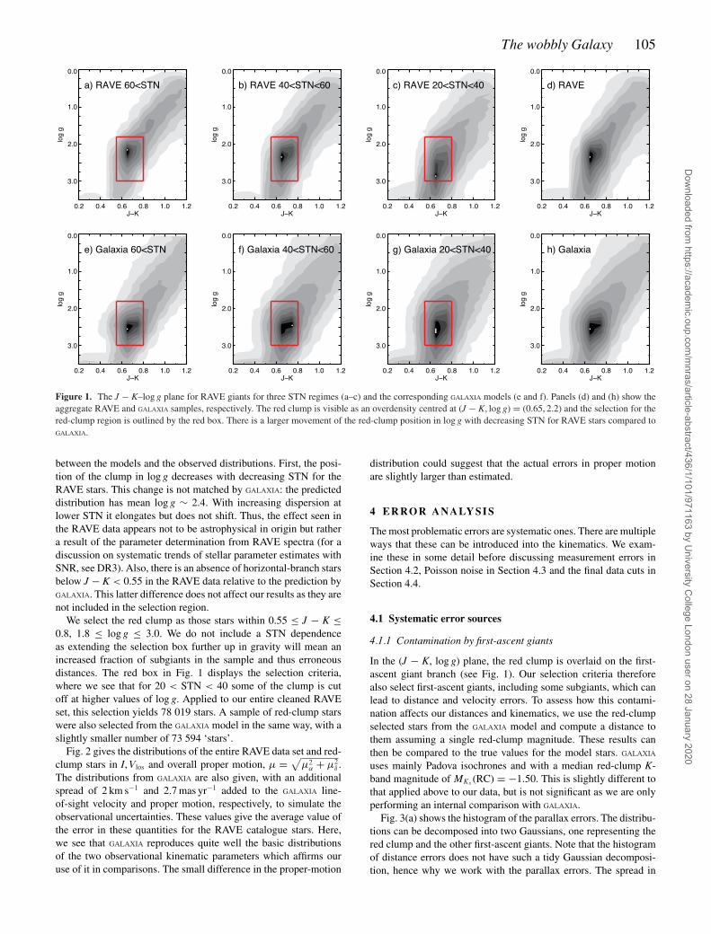
Fig. 1 plots the (J − K, log g) plane for the RAVE giants within8 < I < 13 in the three STN regimes along with the correspondingGALAXIA predictions including errors. Here, we see the clump atJ − K ∼ 0.65 and log g ∼ 2.2. There are some notable differences
Dow
nloaded from https://academ
ic.oup.com/m
nras/article-abstract/436/1/101/971163 by University C
ollege London user on 28 January 2020
The wobbly Galaxy 105
Figure 1. The J − K–log g plane for RAVE giants for three STN regimes (a–c) and the corresponding GALAXIA models (e and f). Panels (d) and (h) show theaggregate RAVE and GALAXIA samples, respectively. The red clump is visible as an overdensity centred at (J − K, log g) = (0.65, 2.2) and the selection for thered-clump region is outlined by the red box. There is a larger movement of the red-clump position in log g with decreasing STN for RAVE stars compared toGALAXIA.
between the models and the observed distributions. First, the posi-tion of the clump in log g decreases with decreasing STN for theRAVE stars. This change is not matched by GALAXIA: the predicteddistribution has mean log g ∼ 2.4. With increasing dispersion atlower STN it elongates but does not shift. Thus, the effect seen inthe RAVE data appears not to be astrophysical in origin but rathera result of the parameter determination from RAVE spectra (for adiscussion on systematic trends of stellar parameter estimates withSNR, see DR3). Also, there is an absence of horizontal-branch starsbelow J − K < 0.55 in the RAVE data relative to the prediction byGALAXIA. This latter difference does not affect our results as they arenot included in the selection region.
We select the red clump as those stars within 0.55 ≤ J − K ≤0.8, 1.8 ≤ log g ≤ 3.0. We do not include a STN dependenceas extending the selection box further up in gravity will mean anincreased fraction of subgiants in the sample and thus erroneousdistances. The red box in Fig. 1 displays the selection criteria,where we see that for 20 < STN < 40 some of the clump is cutoff at higher values of log g. Applied to our entire cleaned RAVEset, this selection yields 78 019 stars. A sample of red-clump starswere also selected from the GALAXIA model in the same way, with aslightly smaller number of 73 594 ‘stars’.
Fig. 2 gives the distributions of the entire RAVE data set and red-clump stars in I, Vlos and overall proper motion, μ =
√μ2
α + μ2δ .
The distributions from GALAXIA are also given, with an additionalspread of 2 km s−1 and 2.7 mas yr−1 added to the GALAXIA line-of-sight velocity and proper motion, respectively, to simulate theobservational uncertainties. These values give the average value ofthe error in these quantities for the RAVE catalogue stars. Here,we see that GALAXIA reproduces quite well the basic distributionsof the two observational kinematic parameters which affirms ouruse of it in comparisons. The small difference in the proper-motion
distribution could suggest that the actual errors in proper motionare slightly larger than estimated.
4 E R RO R A NA LY S I S
The most problematic errors are systematic ones. There are multipleways that these can be introduced into the kinematics. We exam-ine these in some detail before discussing measurement errors inSection 4.2, Poisson noise in Section 4.3 and the final data cuts inSection 4.4.
4.1 Systematic error sources
4.1.1 Contamination by first-ascent giants
In the (J − K, log g) plane, the red clump is overlaid on the first-ascent giant branch (see Fig. 1). Our selection criteria thereforealso select first-ascent giants, including some subgiants, which canlead to distance and velocity errors. To assess how this contami-nation affects our distances and kinematics, we use the red-clumpselected stars from the GALAXIA model and compute a distance tothem assuming a single red-clump magnitude. These results canthen be compared to the true values for the model stars. GALAXIA
uses mainly Padova isochrones and with a median red-clump K-band magnitude of MKs (RC) = −1.50. This is slightly different tothat applied above to our data, but is not significant as we are onlyperforming an internal comparison with GALAXIA.
Fig. 3(a) shows the histogram of the parallax errors. The distribu-tions can be decomposed into two Gaussians, one representing thered clump and the other first-ascent giants. Note that the histogramof distance errors does not have such a tidy Gaussian decomposi-tion, hence why we work with the parallax errors. The spread in
Dow
nloaded from https://academ
ic.oup.com/m
nras/article-abstract/436/1/101/971163 by University C
ollege London user on 28 January 2020
106 M. E. K. Williams et al.
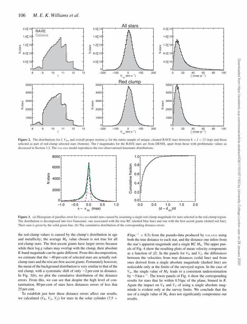
Figure 2. The distributions for I, Vlos and overall proper motion μ for the entire sample of unique, cleaned RAVE stars between 8 < I < 13 (top) and thoseselected as part of red-clump selected stars (bottom). The I magnitudes for the RAVE stars are from DENIS, apart from those with problematic values asdiscussed in Section 3.2. The GALAXIA model reproduces the two observational kinematic distributions.
Figure 3. (a) Histogram of parallax error for GALAXIA model stars caused by assuming a single red-clump magnitude for stars selected in the red-clump region.The distribution is decomposed into two Gaussians: one associated with the true RC (dashed blue line) and one with the first ascent giants (dotted red line).Their sum is given by the solid green line. (b) The cumulative distribution of the corresponding distance errors.
the red-clump values is caused by the clump’s distribution in ageand metallicity; the average MK value chosen is not true for allred-clump stars. The first-ascent giants have larger errors becausewhile their log g values may overlap with the clump, their absoluteK-band magnitude can be quite different. From this decomposition,we estimate that the ∼40 per cent of selected stars are actually red-clump stars and the rest are first-ascent giants. Fortunately however,the mean of the background distribution is very similar to that of thered clump, with a systematic shift of only ∼2 per cent in distance.In Fig. 3(b), we plot the cumulative distribution of the distanceerrors. From this, we can see that despite the high level of con-tamination, 80 per cent of stars have distances errors of less that25 per cent.
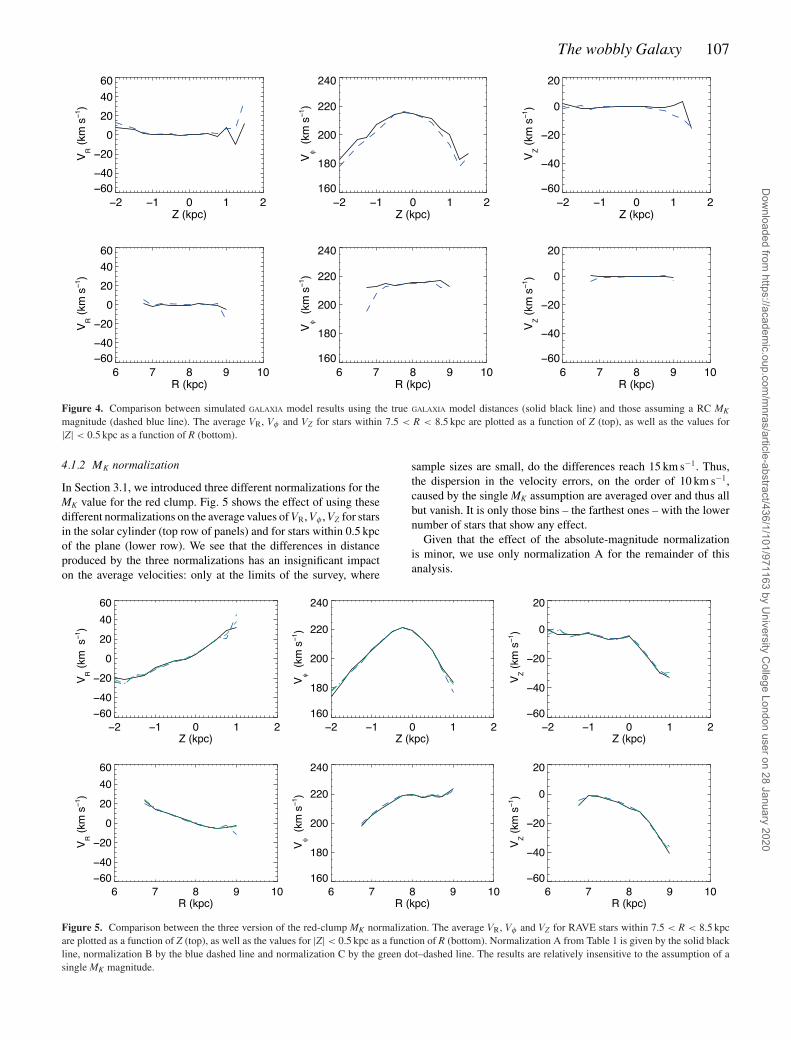
To establish just how these distance errors affect our results,we calculated (VR, Vφ , VZ) for stars in the solar cylinder (7.5 <
R kpc−1 < 8.5) from the pseudo-data produced by GALAXIA usingboth the true distance to each star, and the distance one infers fromthe star’s apparent magnitude and a single RC MK. The upper pan-els of Fig. 4 show the resulting plots of mean velocity componentsas a function of |Z|. In the panels for VR and VZ, the differencesbetween the velocities from true distances (solid line) and fromones derived from a single absolute magnitude (dashed line) arenoticeable only at the limits of the surveyed region. In the case ofVφ , the single value of MK leads to a consistent underestimationby ∼5 km s−1. The lower panels of Fig. 4 show the correspondingresults for stars that lie within 0.5 kpc of the plane, binned in R.Again the impact on VR and VZ of using a single absolute mag-nitude is evident only at the survey limits. We conclude that theuse of a single value of MK does not significantly compromise ourresults.
Dow
nloaded from https://academ
ic.oup.com/m
nras/article-abstract/436/1/101/971163 by University C
ollege London user on 28 January 2020
The wobbly Galaxy 107
Figure 4. Comparison between simulated GALAXIA model results using the true GALAXIA model distances (solid black line) and those assuming a RC MK
magnitude (dashed blue line). The average VR, Vφ and VZ for stars within 7.5 < R < 8.5 kpc are plotted as a function of Z (top), as well as the values for|Z| < 0.5 kpc as a function of R (bottom).
4.1.2 MK normalization
In Section 3.1, we introduced three different normalizations for theMK value for the red clump. Fig. 5 shows the effect of using thesedifferent normalizations on the average values of VR, Vφ , VZ for starsin the solar cylinder (top row of panels) and for stars within 0.5 kpcof the plane (lower row). We see that the differences in distanceproduced by the three normalizations has an insignificant impacton the average velocities: only at the limits of the survey, where
sample sizes are small, do the differences reach 15 km s−1. Thus,the dispersion in the velocity errors, on the order of 10 km s−1,caused by the single MK assumption are averaged over and thus allbut vanish. It is only those bins – the farthest ones – with the lowernumber of stars that show any effect.
Given that the effect of the absolute-magnitude normalizationis minor, we use only normalization A for the remainder of thisanalysis.
Figure 5. Comparison between the three version of the red-clump MK normalization. The average VR, Vφ and VZ for RAVE stars within 7.5 < R < 8.5 kpcare plotted as a function of Z (top), as well as the values for |Z| < 0.5 kpc as a function of R (bottom). Normalization A from Table 1 is given by the solid blackline, normalization B by the blue dashed line and normalization C by the green dot–dashed line. The results are relatively insensitive to the assumption of asingle MK magnitude.
Dow
nloaded from https://academ
ic.oup.com/m
nras/article-abstract/436/1/101/971163 by University C
ollege London user on 28 January 2020
108 M. E. K. Williams et al.
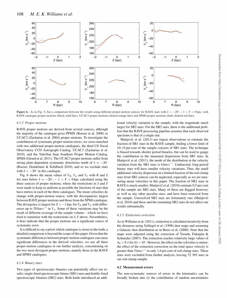
Figure 6. As in Fig. 5, but a comparison between the results using different proper-motion sources for RAVE stars with δ < −20◦, −1 < Y < 0 kpc, withRAVE catalogue proper motions (black solid line), UCAC3 proper motions (dotted orange line) and SPM4 proper motions (dash–dottted red line).
4.1.3 Proper motions
RAVE proper motions are derived from several sources, althoughthe majority of the catalogue gives PPMX (Roeser et al. 2008) orUCAC2 (Zacharias et al. 2004) proper motions. To investigate thecontribution of systematic proper-motion errors, we cross-matchedwith two additional proper-motion catalogues, the third US NavalObservatory CCD Astrograph Catalog, UCAC3 (Zacharias et al.2010), and the Yale/San Juan Southern Proper Motion Catalog,SPM4 (Girard et al. 2011). The UCAC3 proper motions suffer fromstrong plate-dependent systematic distortions north of δ = −20◦
(Roeser, Demleitner & Schilbach 2010), and so we exclude starswith δ > −20◦ in this catalogue.
Fig. 6 shows the mean values of VR, Vφ and VZ with R and Zfor stars below δ = −20◦, − 1 < Y < 0 kpc calculated using thethree sources of proper motions, where the restrictions in δ and Ywere made to keep as uniform as possible the fractions of stars thathave entries in each of the three catalogues. The mean velocities dochange with proper-motion source, with the discrepancies largestbetween RAVE proper motions and those from the SPM4 catalogue.The divergence is largest for Z < −1 kpc for VR and Vφ with differ-ences up to 20 km s−1 in Vφ . Some of these variations may be theresult of different coverage of the sample volume – which we havetried to minimize with the restrictions on δ, Y above. Nevertheless,it does indicate that the proper motions are a significant source ofsystematic error.
It is difficult to say a priori which catalogue is closer to the truth; adetailed comparison is beyond the scope of this paper. Given that thesystematic differences between proper-motion catalogues can causesignificant differences in the derived velocities, we use all threeproper-motion catalogues in our further analysis, concentrating onthe two most divergent proper motions, namely those in the RAVEand SPM4 catalogues.
4.1.4 Binary stars
Two types of spectroscopic binaries can potentially affect our re-sults; single-lined spectroscopic binary (SB1) stars and double-linedspectroscopic binaries (SB2) stars. Both kinds introduced an addi-
tional velocity variation to the sample, with the magnitude muchlarger for SB2 stars. For the SB2 stars, there is the additional prob-lem that the RAVE processing pipeline assumes that each observedspectrum is that of a single star.
Matijevic et al. (2011) use repeat observations to estimate thefraction of SB1 stars in the RAVE sample, finding a lower limit of10–15 per cent of the sample consists of SB1 stars. The techniqueis biased towards shorter period binaries, but can be used to gaugethe contribution to the measured dispersions from SB1 stars. InMatijevic et al. (2011), the mode of the distribution in the velocityvariation from the SB1 stars is 6 km s−1. Undetected, long-periodbinary stars will have smaller velocity variations. Thus, the smalladditional velocity dispersion on a limited fraction of the red-clumpstars from SB1 sources can be neglected, especially as we are mea-suring mean velocities in this paper. The fraction of SB2 stars inRAVE is much smaller; Matijevic et al. (2010) estimate 0.5 per centof the sample are SB2 stars. Many of these are flagged however,as well as any other peculiar stars, and have been removed fromthe sample. Unresolved SB2 stars are fortunately rare (Matijevicet al. 2010) and these and the remaining SB2 stars do not affect ourresults substantially.
4.1.5 Extinction correction
As in Williams et al. (2011), extinction is calculated iteratively fromthe distances using Schlegel et al. (1998) dust maps and assuminga Galactic dust distribution as in Beers et al. (2000). Note that themaps were adjusted using the correction of Yasuda, Fukugita &Schneider (2007). The extinction reaches relatively large values ofAK > 0.1 for |b|< 10◦. However, the effect on the velocities is minor;the effect of the extinction correction on the total space velocity isgreater than 5 km s−1 in only 1.6 per cent of red-clump stars. Thesestars were excluded from further analysis, leaving 72 365 stars inour red-clump sample.
4.2 Measurement errors
The non-systematic sources of errors in the kinematics can bebroadly broken into (i) the contribution of random uncertainties
Dow
nloaded from https://academ
ic.oup.com/m
nras/article-abstract/436/1/101/971163 by University C
ollege London user on 28 January 2020
The wobbly Galaxy 109
Table 3. Cuts on the data adopted for this data analysis.
Cut Reason
√(V 2
R + (Vφ − 220)2 + V 2Z) < 600 km s−1 Remove outlier velocities
|Vφ − 220| < 600 km s−1 Remove outlier velocitieseμα , eμδ < 20 mas yr−1 Remove outlier proper motionsμα , μδ < 400 mas yr−1 Remove high proper-motion starsed/d < 1 Zwitter only, remove large distance error stars
in the measurements and (ii) the finite sample size for each volumebin. We will examine each of these in turn, before discussing anykinematic cuts that were applied to the data.
The Monte Carlo method of error propagation enables an easytracking of error covariances, so we employ it here by generating adistribution of 100 test particles around each input value of distance,proper motion, line-of-sight velocity2 and then calculating the re-sulting points in (VR, Vφ , VZ). We assume that the proper motionsand line-of-sight velocities have Gaussian errors with standard de-viations given by the formal errors for each star. For the distributionin distance for each star however, we generate a double-Gaussiandistribution in the parallax as in Fig. 3, which we then invert toderive the distance distribution. This takes into account the fact thaterrors in distance are due both to the intrinsic width of the RC andthe misclassification of other giants. The ratio between the RC andfirst-ascent giants for GALAXIA model stars changes with distance,where we found a smaller amount of contaminants for d > 1 kpc.The double-Gaussian in parallax then has dispersions (0.05,0.26) mas at a ratio of 2: 1 for d ≤ 1 kpc and 4: 1 for d > 1 kpc.
4.3 Poisson noise
In each of the bins that are used to calculate the mean velocities,there are a finite number of stars N, so Poisson noise contributesto the errors in the derived kinematic properties. These errors scaleas 1/
√N . To establish the error contribution from this source, we
used Bootstrap case resampling with replacement: for each kine-matic quantity, we derived a distribution in the values by randomlyresampling from the distribution of values in the bin. The variancein each value could then be calculated from the resulting distribu-tion. Poisson errors can dominate over measurement errors in binsat large distances that contain very few stars.
To ensure that Poisson errors do not dominate our plots, we onlyuse bins which have Nstars > 50 and only include those points thathave errors in the mean of less than 5 km s−1 (see Section 4.4).
4.4 Data cuts
There are several ways in which to prune the data to those thatare deemed more reliable. However, pruning is liable to introducekinematic biases. We investigated the effects on the measured ve-locities of trimming data via (a) proper motion, (b) error in propermotion, (c) distance errors, (d) magnitude of total velocity and (e)total velocity error, eVtotal. In general, we found that as we increasethe cut-off point, there is a steady increase in velocity dispersionand fluctuations in the average velocity, asymptotically approach-ing a value as the number of stars approaches the full sample. It
2 The positions of the stars are assumed to have negligible errors.
is therefore difficult to justify cuts that remove a significant pro-portion of stars. We therefore introduced cuts that remove only theoutlier values, as given in Table 3, and we do not perform a cut oneVtotal.
Since we seek only to follow trends with R, Z, we do not dis-tinguish between halo, thick- and thin-disc stars. The cuts in totalvelocity therefore aim to be inclusive of halo stars; the 600 km s−1
limit is ∼3σ the halo dispersion of 213 km s−1 (Vallenari et al.2006). An additional cut in Vφ is also introduced to limit ourselvesto stars that have plausible rotation velocities.
In our analysis, we bin the data in physical space, calculating themeans and dispersion in each bin. A further data cut was performedpost-binning. For each bin, we calculate the mean 〈VR〉, 〈Vφ〉, 〈VZ〉.For each of these we also calculate an error in the mean, given bystandard error propagation as
e〈Vq 〉 = 1
N
√∑e2Vq ,i , (1)
where q = R, φ, Z and i = 1, . . . , N, with N the number of starsin the average. The values eVq ,i are given by the MC propagationdescribed in Section 4.2. We remove bins with large errors, i.e.e〈Vq 〉 > 5 km s−1. This affects only peripheral points at large dis-tances from the Sun.
5 SPAT I A L D I S T R I BU T I O N
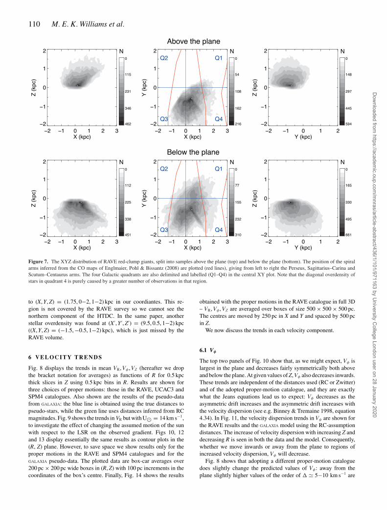
Before examining the velocity trends it is helpful to examine the spa-tial distribution, to see which regions the RAVE red-clump selectionfunction samples. Fig. 7 gives the XYZ distribution for the RAVEred-clump stars, where we have differentiated between stars aboveand below the plane for clarity. Due to RAVE’s magnitude limit, thered-clump stars sample a region between 0.3 < d < 2.8 kpc. This,combined with RAVE’s uneven sky coverage between the Northernand Southern Galactic hemispheres, means that the sample regionis mostly outside d > 0.5 kpc and quadrants 1 and 2 above the planeare not sampled.
As in S11 and S12, we also plot the location of the spiral arms asinferred from the CO maps of Englmaier et al. (2008). Going fromouter to inner (left to right), the arms are the Perseus, Sagittarius–Carina and Scutum–Centaurus arms. We see that our sample missesthe Scutum–Centaurus arms entirely, and samples above and belowthe other two spiral arms.
Another significant nearby feature is the HTDC (Larsen &Humphreys 1996 and Parker et al. 2003). Parker et al. (2003)detected it via star counts in the region l = ±(20◦−55)◦ bothabove and below the plane at latitudes b = ±(25◦−45)◦. This isin quadrant 1. Recently, Larsen, Cabenela & Humphreys (2011)reported that the HTDC starts at (X, Y) = (0.5, 0.5) kpc in ourcoordinates, for 0.5 < |Z| < 1.0 kpc. From Fig. 7, we can seethat the RAVE sample in the south intersects with this loca-tion of the HTDC. Juric et al. (2008) also found the HTDC inthe location (X′, Y′, Z′) = (6.25, −2−0, 1−2) kpc, corresponding
Dow
nloaded from https://academ
ic.oup.com/m
nras/article-abstract/436/1/101/971163 by University C
ollege London user on 28 January 2020
110 M. E. K. Williams et al.
Figure 7. The XYZ distribution of RAVE red-clump giants, split into samples above the plane (top) and below the plane (bottom). The position of the spiralarms inferred from the CO maps of Englmaier, Pohl & Bissantz (2008) are plotted (red lines), giving from left to right the Perseus, Sagittarius–Carina andScutum–Centaurus arms. The four Galactic quadrants are also delimited and labelled (Q1–Q4) in the central XY plot. Note that the diagonal overdensity ofstars in quadrant 4 is purely caused by a greater number of observations in that region.
to (X, Y, Z) = (1.75, 0−2, 1−2) kpc in our coordiantes. This re-gion is not covered by the RAVE survey so we cannot see thenorthern component of the HTDC. In the same paper, anotherstellar overdensity was found at (X′, Y′, Z′) = (9.5, 0.5, 1−2) kpc((X, Y, Z) = (−1.5, −0.5, 1−2) kpc), which is just missed by theRAVE volume.
6 V E L O C I T Y T R E N D S
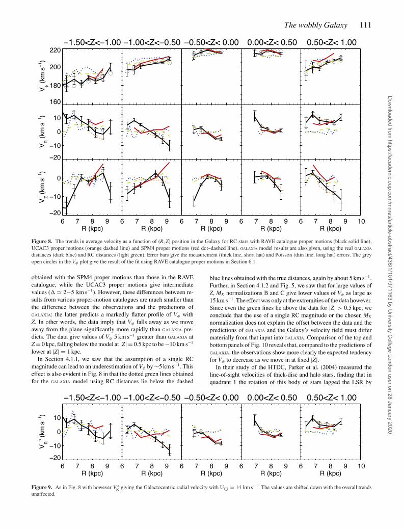
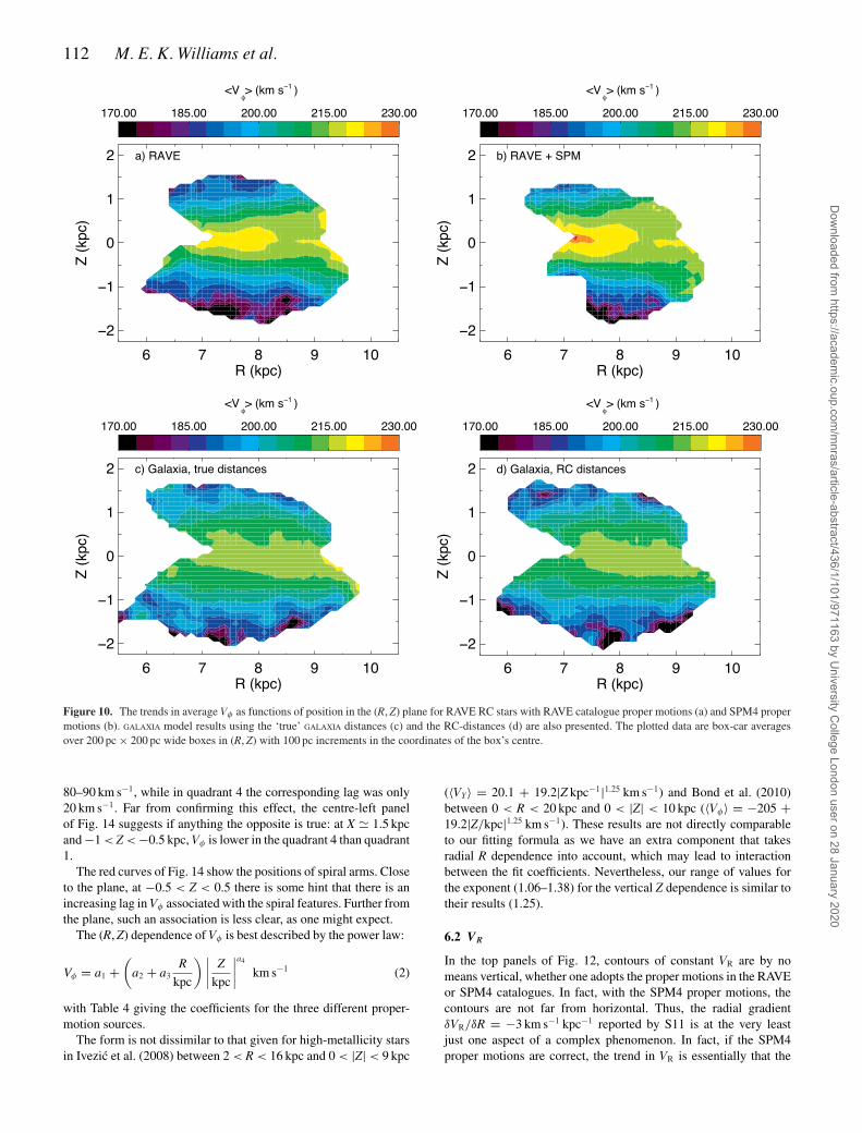
Fig. 8 displays the trends in mean VR, Vφ , VZ (hereafter we dropthe bracket notation for averages) as functions of R for 0.5 kpcthick slices in Z using 0.5 kpc bins in R. Results are shown forthree choices of proper motions: those in the RAVE, UCAC3 andSPM4 catalogues. Also shown are the results of the pseudo-datafrom GALAXIA: the blue line is obtained using the true distances topseudo-stars, while the green line uses distances inferred from RCmagnitudes. Fig. 9 shows the trends in VR but with U� = 14 km s−1,to investigate the effect of changing the assumed motion of the sunwith respect to the LSR on the observed gradient. Figs 10, 12and 13 display essentially the same results as contour plots in the(R, Z) plane. However, to save space we show results only for theproper motions in the RAVE and SPM4 catalogues and for theGALAXIA pseudo-data. The plotted data are box-car averages over200 pc × 200 pc wide boxes in (R, Z) with 100 pc increments in thecoordinates of the box’s centre. Finally, Fig. 14 shows the results
obtained with the proper motions in the RAVE catalogue in full 3D– VR, Vφ , VZ are averaged over boxes of size 500 × 500 × 500 pc.The centres are moved by 250 pc in X and Y and spaced by 500 pcin Z.
We now discuss the trends in each velocity component.
6.1 Vφ
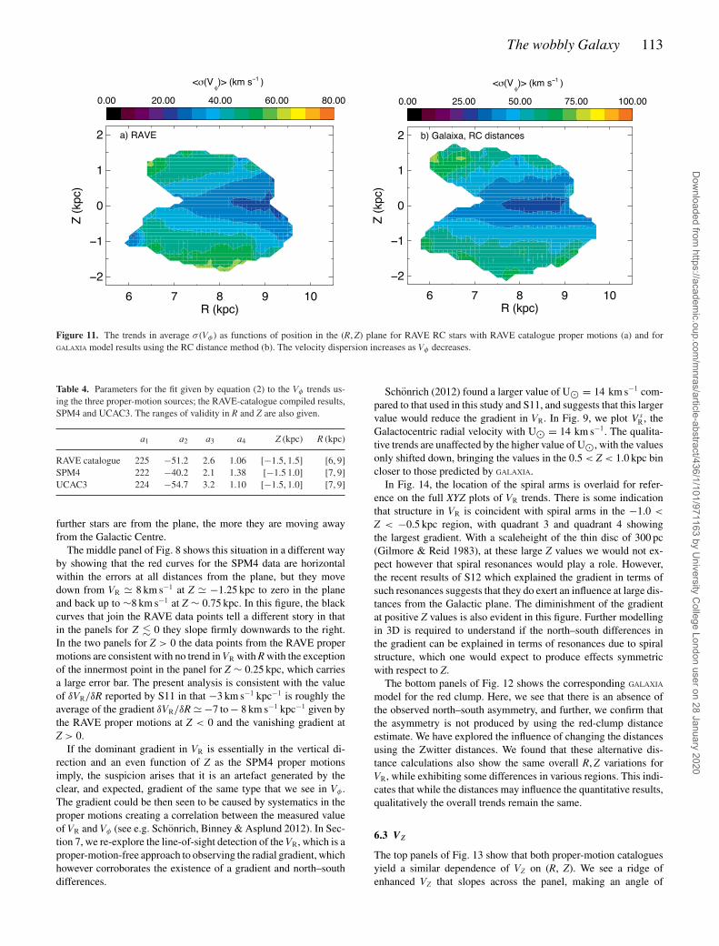
The top two panels of Fig. 10 show that, as we might expect, Vφ islargest in the plane and decreases fairly symmetrically both aboveand below the plane. At given values of Z, Vφ also decreases inwards.These trends are independent of the distances used (RC or Zwitter)and of the adopted proper-motion catalogue, and they are exactlywhat the Jeans equations lead us to expect: Vφ decreases as theasymmetric drift increases and the asymmetric drift increases withthe velocity dispersion (see e.g. Binney & Tremaine 1998, equation4.34). In Fig. 11, the velocity dispersion trends in Vφ are shown forthe RAVE results and the GALAXIA model using the RC-assumptiondistances. The increase of velocity dispersion with increasing Z anddecreasing R is seen in both the data and the model. Consequently,whether we move inwards or away from the plane to regions ofincreased velocity dispersion, Vφ will decrease.
Fig. 8 shows that adopting a different proper-motion cataloguedoes slightly change the predicted values of Vφ : away from theplane slightly higher values of the order of � � 5−10 km s−1 are
Dow
nloaded from https://academ
ic.oup.com/m
nras/article-abstract/436/1/101/971163 by University C
ollege London user on 28 January 2020
The wobbly Galaxy 111
Figure 8. The trends in average velocity as a function of (R, Z) position in the Galaxy for RC stars with RAVE catalogue proper motions (black solid line),UCAC3 proper motions (orange dashed line) and SPM4 proper motions (red dot–dashed line). GALAXIA model results are also given, using the real GALAXIA
distances (dark blue) and RC distances (light green). Error bars give the measurement (thick line, short hat) and Poisson (thin line, long hat) errors. The greyopen circles in the Vφ plot give the result of the fit using RAVE catalogue proper motions in Section 6.1.
obtained with the SPM4 proper motions than those in the RAVEcatalogue, while the UCAC3 proper motions give intermediatevalues (� � 2−5 km s−1). However, these differences between re-sults from various proper-motion catalogues are much smaller thanthe difference between the observations and the predictions ofGALAXIA: the latter predicts a markedly flatter profile of Vφ withZ. In other words, the data imply that Vφ falls away as we moveaway from the plane significantly more rapidly than GALAXIA pre-dicts. The data give values of Vφ 5 km s−1 greater than GALAXIA atZ = 0 kpc, falling below the model at |Z| = 0.5 kpc to be −10 km s−1
lower at |Z| = 1 kpc.In Section 4.1.1, we saw that the assumption of a single RC
magnitude can lead to an underestimation of Vφ by ∼5 km s−1. Thiseffect is also evident in Fig. 8 in that the dotted green lines obtainedfor the GALAXIA model using RC distances lie below the dashed
blue lines obtained with the true distances, again by about 5 km s−1.Further, in Section 4.1.2 and Fig. 5, we saw that for large values ofZ, MK normalizations B and C give lower values of Vφ as large as15 km s−1. The effect was only at the extremities of the data however.Since even the green lines lie above the data for |Z| > 0.5 kpc, weconclude that the use of a single RC magnitude or the chosen MK
normalization does not explain the offset between the data and thepredictions of GALAXIA and the Galaxy’s velocity field must differmaterially from that input into GALAXIA. Comparison of the top andbottom panels of Fig. 10 reveals that, compared to the predictions ofGALAXIA, the observations show more clearly the expected tendencyfor Vφ to decrease as we move in at fixed |Z|.
In their study of the HTDC, Parker et al. (2004) measured theline-of-sight velocities of thick-disc and halo stars, finding that inquadrant 1 the rotation of this body of stars lagged the LSR by
Figure 9. As in Fig. 8 with however V sR giving the Galactocentric radial velocity with U� = 14 km s−1. The values are shifted down with the overall trends
unaffected.
Dow
nloaded from https://academ
ic.oup.com/m
nras/article-abstract/436/1/101/971163 by University C
ollege London user on 28 January 2020
112 M. E. K. Williams et al.
Figure 10. The trends in average Vφ as functions of position in the (R, Z) plane for RAVE RC stars with RAVE catalogue proper motions (a) and SPM4 propermotions (b). GALAXIA model results using the ‘true’ GALAXIA distances (c) and the RC-distances (d) are also presented. The plotted data are box-car averagesover 200 pc × 200 pc wide boxes in (R, Z) with 100 pc increments in the coordinates of the box’s centre.
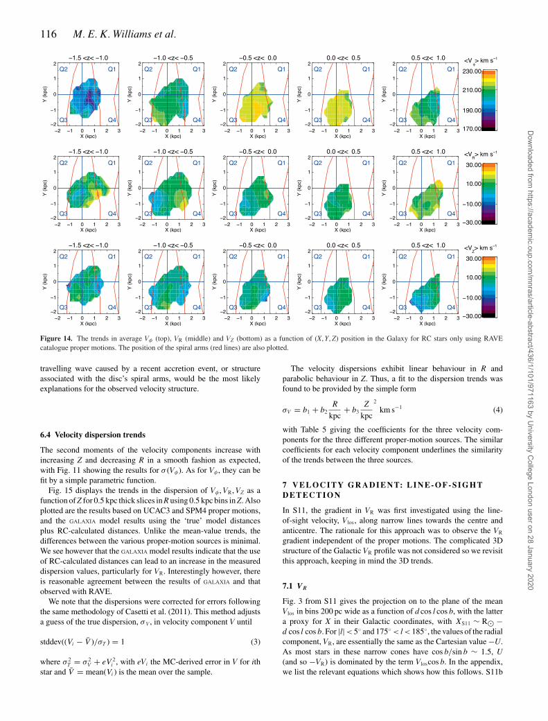
80–90 km s−1, while in quadrant 4 the corresponding lag was only20 km s−1. Far from confirming this effect, the centre-left panelof Fig. 14 suggests if anything the opposite is true: at X � 1.5 kpcand −1 < Z < −0.5 kpc, Vφ is lower in the quadrant 4 than quadrant1.
The red curves of Fig. 14 show the positions of spiral arms. Closeto the plane, at −0.5 < Z < 0.5 there is some hint that there is anincreasing lag in Vφ associated with the spiral features. Further fromthe plane, such an association is less clear, as one might expect.
The (R, Z) dependence of Vφ is best described by the power law:
Vφ = a1 +(
a2 + a3R
kpc
) ∣∣∣∣ Z
kpc
∣∣∣∣a4
km s−1 (2)
with Table 4 giving the coefficients for the three different proper-motion sources.
The form is not dissimilar to that given for high-metallicity starsin Ivezic et al. (2008) between 2 < R < 16 kpc and 0 < |Z| < 9 kpc
(〈VY〉 = 20.1 + 19.2|Z kpc−1|1.25 km s−1) and Bond et al. (2010)between 0 < R < 20 kpc and 0 < |Z| < 10 kpc (〈Vφ〉 = −205 +19.2|Z/kpc|1.25 km s−1). These results are not directly comparableto our fitting formula as we have an extra component that takesradial R dependence into account, which may lead to interactionbetween the fit coefficients. Nevertheless, our range of values forthe exponent (1.06–1.38) for the vertical Z dependence is similar totheir results (1.25).
6.2 VR
In the top panels of Fig. 12, contours of constant VR are by nomeans vertical, whether one adopts the proper motions in the RAVEor SPM4 catalogues. In fact, with the SPM4 proper motions, thecontours are not far from horizontal. Thus, the radial gradientδVR/δR = −3 km s−1 kpc−1 reported by S11 is at the very leastjust one aspect of a complex phenomenon. In fact, if the SPM4proper motions are correct, the trend in VR is essentially that the
Dow
nloaded from https://academ
ic.oup.com/m
nras/article-abstract/436/1/101/971163 by University C
ollege London user on 28 January 2020
The wobbly Galaxy 113
Figure 11. The trends in average σ (Vφ ) as functions of position in the (R, Z) plane for RAVE RC stars with RAVE catalogue proper motions (a) and forGALAXIA model results using the RC distance method (b). The velocity dispersion increases as Vφ decreases.
Table 4. Parameters for the fit given by equation (2) to the Vφ trends us-ing the three proper-motion sources; the RAVE-catalogue compiled results,SPM4 and UCAC3. The ranges of validity in R and Z are also given.
a1 a2 a3 a4 Z (kpc) R (kpc)
RAVE catalogue 225 −51.2 2.6 1.06 [−1.5, 1.5] [6, 9]SPM4 222 −40.2 2.1 1.38 [−1.5 1.0] [7, 9]UCAC3 224 −54.7 3.2 1.10 [−1.5, 1.0] [7, 9]
further stars are from the plane, the more they are moving awayfrom the Galactic Centre.
The middle panel of Fig. 8 shows this situation in a different wayby showing that the red curves for the SPM4 data are horizontalwithin the errors at all distances from the plane, but they movedown from VR � 8 km s−1 at Z � −1.25 kpc to zero in the planeand back up to ∼8 km s−1 at Z ∼ 0.75 kpc. In this figure, the blackcurves that join the RAVE data points tell a different story in thatin the panels for Z � 0 they slope firmly downwards to the right.In the two panels for Z > 0 the data points from the RAVE propermotions are consistent with no trend in VR with R with the exceptionof the innermost point in the panel for Z ∼ 0.25 kpc, which carriesa large error bar. The present analysis is consistent with the valueof δVR/δR reported by S11 in that −3 km s−1 kpc−1 is roughly theaverage of the gradient δVR/δR � −7 to − 8 km s−1 kpc−1 given bythe RAVE proper motions at Z < 0 and the vanishing gradient atZ > 0.
If the dominant gradient in VR is essentially in the vertical di-rection and an even function of Z as the SPM4 proper motionsimply, the suspicion arises that it is an artefact generated by theclear, and expected, gradient of the same type that we see in Vφ .The gradient could be then seen to be caused by systematics in theproper motions creating a correlation between the measured valueof VR and Vφ (see e.g. Schonrich, Binney & Asplund 2012). In Sec-tion 7, we re-explore the line-of-sight detection of the VR, which is aproper-motion-free approach to observing the radial gradient, whichhowever corroborates the existence of a gradient and north–southdifferences.
Schonrich (2012) found a larger value of U� = 14 km s−1 com-pared to that used in this study and S11, and suggests that this largervalue would reduce the gradient in VR. In Fig. 9, we plot V s
R, theGalactocentric radial velocity with U� = 14 km s−1. The qualita-tive trends are unaffected by the higher value of U�, with the valuesonly shifted down, bringing the values in the 0.5 < Z < 1.0 kpc bincloser to those predicted by GALAXIA.
In Fig. 14, the location of the spiral arms is overlaid for refer-ence on the full XYZ plots of VR trends. There is some indicationthat structure in VR is coincident with spiral arms in the −1.0 <
Z < −0.5 kpc region, with quadrant 3 and quadrant 4 showingthe largest gradient. With a scaleheight of the thin disc of 300 pc(Gilmore & Reid 1983), at these large Z values we would not ex-pect however that spiral resonances would play a role. However,the recent results of S12 which explained the gradient in terms ofsuch resonances suggests that they do exert an influence at large dis-tances from the Galactic plane. The diminishment of the gradientat positive Z values is also evident in this figure. Further modellingin 3D is required to understand if the north–south differences inthe gradient can be explained in terms of resonances due to spiralstructure, which one would expect to produce effects symmetricwith respect to Z.
The bottom panels of Fig. 12 shows the corresponding GALAXIA
model for the red clump. Here, we see that there is an absence ofthe observed north–south asymmetry, and further, we confirm thatthe asymmetry is not produced by using the red-clump distanceestimate. We have explored the influence of changing the distancesusing the Zwitter distances. We found that these alternative dis-tance calculations also show the same overall R, Z variations forVR, while exhibiting some differences in various regions. This indi-cates that while the distances may influence the quantitative results,qualitatively the overall trends remain the same.
6.3 VZ
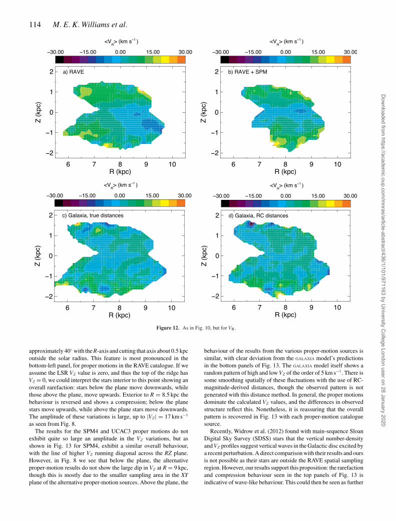
The top panels of Fig. 13 show that both proper-motion cataloguesyield a similar dependence of VZ on (R, Z). We see a ridge ofenhanced VZ that slopes across the panel, making an angle of
Dow
nloaded from https://academ
ic.oup.com/m
nras/article-abstract/436/1/101/971163 by University C
ollege London user on 28 January 2020
114 M. E. K. Williams et al.
Figure 12. As in Fig. 10, but for VR.
approximately 40◦ with the R-axis and cutting that axis about 0.5 kpcoutside the solar radius. This feature is most pronounced in thebottom-left panel, for proper motions in the RAVE catalogue. If weassume the LSR VZ value is zero, and thus the top of the ridge hasVZ = 0, we could interpret the stars interior to this point showing anoverall rarefaction: stars below the plane move downwards, whilethose above the plane, move upwards. Exterior to R = 8.5 kpc thebehaviour is reversed and shows a compression; below the planestars move upwards, while above the plane stars move downwards.The amplitude of these variations is large, up to |VZ| = 17 km s−1
as seen from Fig. 8.The results for the SPM4 and UCAC3 proper motions do not
exhibit quite so large an amplitude in the VZ variations, but asshown in Fig. 13 for SPM4, exhibit a similar overall behaviour,with the line of higher VZ running diagonal across the RZ plane.However, in Fig. 8 we see that below the plane, the alternativeproper-motion results do not show the large dip in VZ at R = 9 kpc,though this is mostly due to the smaller sampling area in the XYplane of the alternative proper-motion sources. Above the plane, the
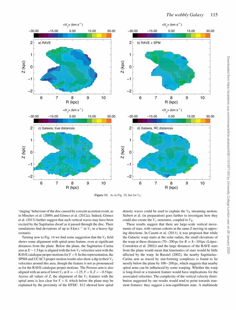
behaviour of the results from the various proper-motion sources issimilar, with clear deviation from the GALAXIA model’s predictionsin the bottom panels of Fig. 13. The GALAXIA model itself shows arandom pattern of high and low VZ of the order of 5 km s−1. There issome smoothing spatially of these fluctuations with the use of RC-magnitude-derived distances, though the observed pattern is notgenerated with this distance method. In general, the proper motionsdominate the calculated VZ values, and the differences in observedstructure reflect this. Nonetheless, it is reassuring that the overallpattern is recovered in Fig. 13 with each proper-motion cataloguesource.
Recently, Widrow et al. (2012) found with main-sequence SloanDigital Sky Survey (SDSS) stars that the vertical number-densityand VZ profiles suggest vertical waves in the Galactic disc excited bya recent perturbation. A direct comparison with their results and oursis not possible as their stars are outside the RAVE spatial samplingregion. However, our results support this proposition: the rarefactionand compression behaviour seen in the top panels of Fig. 13 isindicative of wave-like behaviour. This could then be seen as further
Dow
nloaded from https://academ
ic.oup.com/m
nras/article-abstract/436/1/101/971163 by University C
ollege London user on 28 January 2020
The wobbly Galaxy 115
Figure 13. As in Fig. 10, but for VZ.
‘ringing’ behaviour of the disc caused by a recent accretion event, asin Minchev et al. (2009) and Gomez et al. (2012a). Indeed, Gomezet al. (2013) further suggest that such vertical waves may have beenexcited by the Sagittarius dwarf as it passed through the disc. Theirsimulations find deviations of up to 8 km s−1 in VZ in a heavy-Sgrscenario.
Turning now to Fig. 14 we find some suggestion that the VZ fieldshows some alignment with spiral-arms feature, even at significantdistances from the plane. Below the plane, the Sagittarius–Carinaarm at X ∼ 1.5 kpc is aligned with the low VZ velocities seen with theRAVE catalogue proper motions for Y < 0. In this representation, theSPM4 and UCAC3 proper-motion results also show a dip in their VZ
velocities around this area, though the feature is not as pronouncedas for the RAVE catalogue proper motions. The Perseus arm is alsoaligned with an area of lower VZ at X = −1.25, Y < 0, Z < −0.5 kpc.Across all values of Z, the alignment of the VZ features with thespiral arms is less clear for Y > 0, which below the plane may beexplained by the proximity of the HTDC. S12 showed how spiral
density waves could be used to explain the VR streaming motion.Siebert et al. (in preparation) goes further to investigate how theycould also create the VZ structures, coupled to VR.
These results suggest that there are large-scale vertical move-ments of stars, with various cohorts at the same Z moving in oppos-ing directions. In Casetti et al. (2011), it was proposed that whilethe Galactic warp starts at the solar radius, the small elevations ofthe warp at these distances (70−200 pc for R = 8−10 kpc (Lopez-Corredoira et al. 2002)) and the large distances of the RAVE starsfrom the plane would mean that kinematics of stars would be littleaffected by the warp. In Russiel (2002), the nearby Sagittarius–Carina arm as traced by star-forming complexes is found to liemostly below the plane by 100−200 pc, which suggests that nearbyspiral arms can be influenced by some warping. Whether the warpis long-lived or a transient feature would have implications for theassociated velocities. The complexity of the vertical velocity distri-bution suggested by our results would tend to point towards tran-sient features: they suggest a non-equilibrium state. A multimode
Dow
nloaded from https://academ
ic.oup.com/m
nras/article-abstract/436/1/101/971163 by University C
ollege London user on 28 January 2020
116 M. E. K. Williams et al.
Figure 14. The trends in average Vφ (top), VR (middle) and VZ (bottom) as a function of (X, Y, Z) position in the Galaxy for RC stars only using RAVEcatalogue proper motions. The position of the spiral arms (red lines) are also plotted.
travelling wave caused by a recent accretion event, or structureassociated with the disc’s spiral arms, would be the most likelyexplanations for the observed velocity structure.
6.4 Velocity dispersion trends
The second moments of the velocity components increase withincreasing Z and decreasing R in a smooth fashion as expected,with Fig. 11 showing the results for σ (Vφ). As for Vφ , they can befit by a simple parametric function.
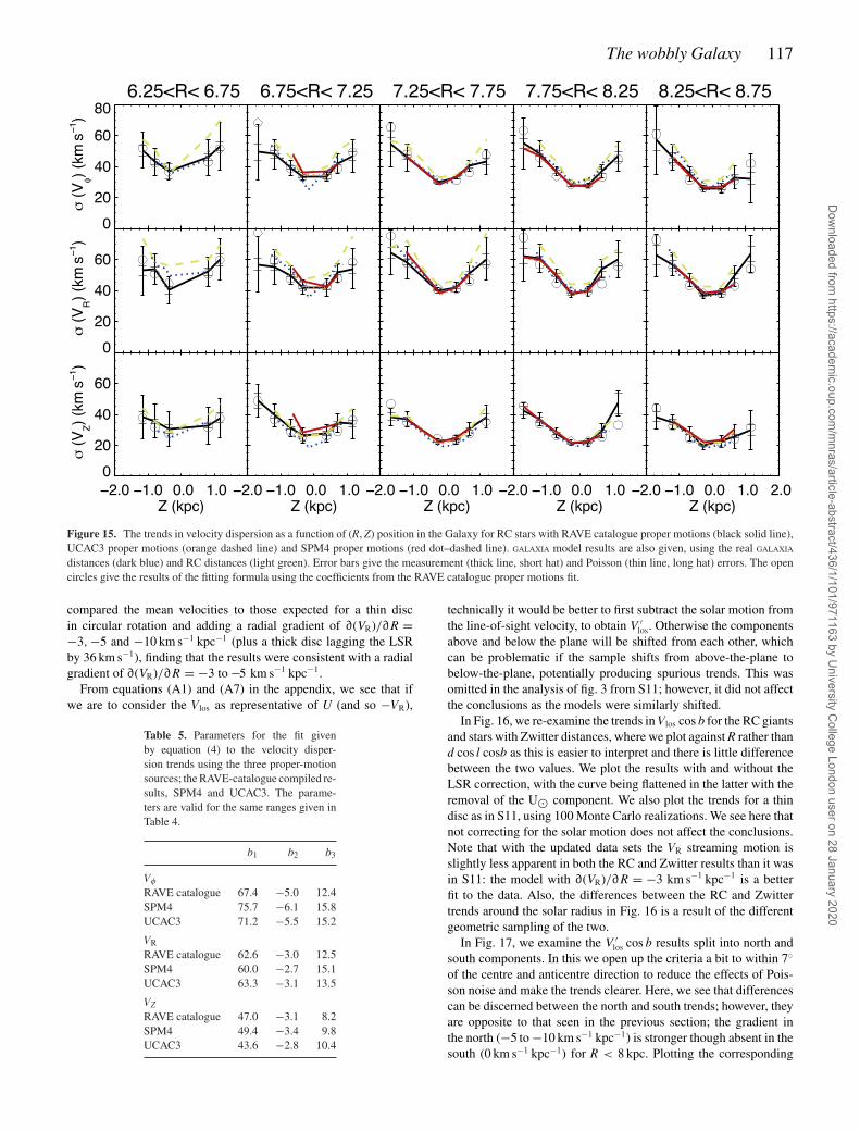
Fig. 15 displays the trends in the dispersion of Vφ , VR, VZ as afunction of Z for 0.5 kpc thick slices in R using 0.5 kpc bins in Z. Alsoplotted are the results based on UCAC3 and SPM4 proper motions,and the GALAXIA model results using the ‘true’ model distancesplus RC-calculated distances. Unlike the mean-value trends, thedifferences between the various proper-motion sources is minimal.We see however that the GALAXIA model results indicate that the useof RC-calculated distances can lead to an increase in the measureddispersion values, particularly for VR. Interestingly however, thereis reasonable agreement between the results of GALAXIA and thatobserved with RAVE.
We note that the dispersions were corrected for errors followingthe same methodology of Casetti et al. (2011). This method adjustsa guess of the true dispersion, σ V, in velocity component V until
stddev((Vi − V )/σT ) = 1 (3)
where σ 2T = σ 2
V + eV 2i , with eVi the MC-derived error in V for ith
star and V = mean(Vi) is the mean over the sample.
The velocity dispersions exhibit linear behaviour in R andparabolic behaviour in Z. Thus, a fit to the dispersion trends wasfound to be provided by the simple form
σV = b1 + b2R
kpc+ b3
Z
kpc
2
km s−1 (4)
with Table 5 giving the coefficients for the three velocity com-ponents for the three different proper-motion sources. The similarcoefficients for each velocity component underlines the similarityof the trends between the three sources.
7 V E L O C I T Y G R A D I E N T: L I N E - O F - S I G H TD E T E C T I O N
In S11, the gradient in VR was first investigated using the line-of-sight velocity, Vlos, along narrow lines towards the centre andanticentre. The rationale for this approach was to observe the VR
gradient independent of the proper motions. The complicated 3Dstructure of the Galactic VR profile was not considered so we revisitthis approach, keeping in mind the 3D trends.
7.1 VR
Fig. 3 from S11 gives the projection on to the plane of the meanVlos in bins 200 pc wide as a function of d cos l cos b, with the lattera proxy for X in their Galactic coordinates, with XS11 ∼ R� −d cos l cos b. For |l|< 5◦ and 175◦ < l < 185◦, the values of the radialcomponent, VR, are essentially the same as the Cartesian value −U.As most stars in these narrow cones have cos b/sin b ∼ 1.5, U(and so −VR) is dominated by the term Vloscos b. In the appendix,we list the relevant equations which shows how this follows. S11b
Dow
nloaded from https://academ
ic.oup.com/m
nras/article-abstract/436/1/101/971163 by University C
ollege London user on 28 January 2020
The wobbly Galaxy 117
Figure 15. The trends in velocity dispersion as a function of (R, Z) position in the Galaxy for RC stars with RAVE catalogue proper motions (black solid line),UCAC3 proper motions (orange dashed line) and SPM4 proper motions (red dot–dashed line). GALAXIA model results are also given, using the real GALAXIA
distances (dark blue) and RC distances (light green). Error bars give the measurement (thick line, short hat) and Poisson (thin line, long hat) errors. The opencircles give the results of the fitting formula using the coefficients from the RAVE catalogue proper motions fit.
compared the mean velocities to those expected for a thin discin circular rotation and adding a radial gradient of ∂(VR)/∂R =−3, −5 and −10 km s−1 kpc−1 (plus a thick disc lagging the LSRby 36 km s−1), finding that the results were consistent with a radialgradient of ∂(VR)/∂R = −3 to −5 km s−1 kpc−1.
From equations (A1) and (A7) in the appendix, we see that ifwe are to consider the Vlos as representative of U (and so −VR),
Table 5. Parameters for the fit givenby equation (4) to the velocity disper-sion trends using the three proper-motionsources; the RAVE-catalogue compiled re-sults, SPM4 and UCAC3. The parame-ters are valid for the same ranges given inTable 4.
b1 b2 b3
Vφ
RAVE catalogue 67.4 −5.0 12.4SPM4 75.7 −6.1 15.8UCAC3 71.2 −5.5 15.2
VR
RAVE catalogue 62.6 −3.0 12.5SPM4 60.0 −2.7 15.1UCAC3 63.3 −3.1 13.5
VZ
RAVE catalogue 47.0 −3.1 8.2SPM4 49.4 −3.4 9.8UCAC3 43.6 −2.8 10.4
technically it would be better to first subtract the solar motion fromthe line-of-sight velocity, to obtain V ′
los. Otherwise the componentsabove and below the plane will be shifted from each other, whichcan be problematic if the sample shifts from above-the-plane tobelow-the-plane, potentially producing spurious trends. This wasomitted in the analysis of fig. 3 from S11; however, it did not affectthe conclusions as the models were similarly shifted.
In Fig. 16, we re-examine the trends in Vlos cos b for the RC giantsand stars with Zwitter distances, where we plot against R rather thand cos l cosb as this is easier to interpret and there is little differencebetween the two values. We plot the results with and without theLSR correction, with the curve being flattened in the latter with theremoval of the U� component. We also plot the trends for a thindisc as in S11, using 100 Monte Carlo realizations. We see here thatnot correcting for the solar motion does not affect the conclusions.Note that with the updated data sets the VR streaming motion isslightly less apparent in both the RC and Zwitter results than it wasin S11: the model with ∂(VR)/∂R = −3 km s−1 kpc−1 is a betterfit to the data. Also, the differences between the RC and Zwittertrends around the solar radius in Fig. 16 is a result of the differentgeometric sampling of the two.
In Fig. 17, we examine the V ′los cos b results split into north and
south components. In this we open up the criteria a bit to within 7◦
of the centre and anticentre direction to reduce the effects of Pois-son noise and make the trends clearer. Here, we see that differencescan be discerned between the north and south trends; however, theyare opposite to that seen in the previous section; the gradient inthe north (−5 to −10 km s−1 kpc−1) is stronger though absent in thesouth (0 km s−1 kpc−1) for R < 8 kpc. Plotting the corresponding
Dow
nloaded from https://academ
ic.oup.com/m
nras/article-abstract/436/1/101/971163 by University C
ollege London user on 28 January 2020

118 M. E. K. Williams et al.
Figure 16. As in fig. 3 of S11, projection of mean RAVE Vlos on the Galacticplane in distance intervals of 200 pc towards the Galactic Centre (|l| < 5◦)and anticentre (175◦ < l < 185◦). Panels (a) and (c) show the results forRC stars with heliocentric line-of-sight velocity and corrected to the LSR,respectively, while (b) and (d) similarly show the Zwitter distance results.The solid curves represent a thin-disc population with a radial velocitygradient of δVR/δR = 0, −3, −5 and −10 km s−1 kpc−1, going from greento purple.
Figure 17. As in the bottom plots of Fig. 16, but for Galactic Centre(|l| < 7◦) and anticentre (173◦ < l < 187◦) and split into above (a, b) andbelow (c, d) the plane.
results for VR in Fig. 18, we find that the including the proper-motion results shifts the overall values so that the northern trendsare more in line with δVZ/δR = −10 km s−1 kpc−1 and the south-ern δVZ/δR = −3 to −5 km s−1 kpc−1. Despite the disparity withthe actual numbers, the cause of which is discussed below, both
Figure 18. Corresponding VR trends to Fig. 17, looking at the GalacticCentre (|l| < 7◦) and anticentre (173◦ < l < 187◦) and split into above(a, b) and below (c, d) the plane.
V ′los cos b and the VR nonetheless exhibit differences between the
north and south trends, opposite to those found in Section 6.2.To understand the reversal of the trends note first that the selected
sample cuts across a range of Z as we change R so these plotscombine the R and Z trends seen previously. Secondly, the necessaryrestriction on l means that we are sampling a very narrow beam andthus do not see the global patterns, but only those along that beam.In Fig. 14, quadrants 3 and 4 show the largest gradient, which wemiss with the beams. Hence, these plots emphasize the 3D natureof the VR values in the solar neighbourhood: what you measurevery much depends on where you look, be it north or south, and atdifferent R and Z values.
7.2 VZ
From equation (A6) in the appendix, we can see that V ′b cos b can be
used as a proxy for W = VZ if |cos b| > |sin b|. This condition is forthe most part met in the low latitudes sampled along the |l| < 7◦ and173◦ < l < 187◦ cones used above. So in Fig. 19, we examine thetrends above and below the plane for V ′
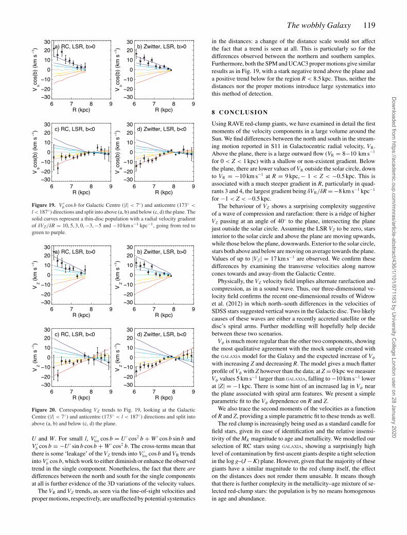
b cos b in these directions,with Fig. 20 giving the corresponding trends in the total VZ. Notethat we use RC and Zwitter distances here to provide the abscissa,supplementing the proper-motion data. We also plot both positiveand negative trends in VZ for a thin-disc model as above, with valuesfrom ∂(VZ)/∂R = −10, −5, −3, 0, 3, 5, 10 km s−1 kpc−1.
Both Figs 19 and 20 show that the trends above and below theplane are markedly different, with the VZ decreasing with R abovethe plane at a rate of ∂(VZ)/∂R ∼ −10 km s−1 kpc−1 according tothe V ′
b cos b plot and −5 km s−1 kpc−1, to the VZ plot. Below theplane, there is a positive trend of ∂(VZ)/∂R ∼ +5 km s−1 kpc−1 inboth plots. This positive trend in VZ appears to stop just beyond thesolar circle at R ∼ 8.5 kpc. In contrast to VR above, this behaviouris consistent with what was found in Section 6.3.
Note that the differences between the observed magnitude ofthe trends in V ′
los cos b and VR, plus V ′b cos b and VZ can be ex-
plained by the fact that both V ′los and V ′
b contain components of
Dow
nloaded from https://academ
ic.oup.com/m
nras/article-abstract/436/1/101/971163 by University C
ollege London user on 28 January 2020
The wobbly Galaxy 119
Figure 19. V ′b cos b for Galactic Centre (|l| < 7◦) and anticentre (173◦ <
l < 187◦) directions and split into above (a, b) and below (c, d) the plane. Thesolid curves represent a thin-disc population with a radial velocity gradientof δVZ/δR = 10, 5, 3, 0, −3, −5 and −10 km s−1 kpc−1, going from red togreen to purple.
Figure 20. Corresponding VZ trends to Fig. 19, looking at the GalacticCentre (|l| < 7◦) and anticentre (173◦ < l < 187◦) directions and split intoabove (a, b) and below (c, d) the plane.
U and W. For small l, V ′los cos b = U ′ cos2 b + W ′ cos b sin b and
V ′b cos b = −U ′ sin b cos b + W ′ cos2 b. The cross-terms mean that
there is some ‘leakage’ of the VZ trends into V ′los cos b and VR trends
into V ′b cos b, which work to either diminish or enhance the observed
trend in the single component. Nonetheless, the fact that there aredifferences between the north and south for the single componentsat all is further evidence of the 3D variations of the velocity values.
The VR and VZ trends, as seen via the line-of-sight velocities andproper motions, respectively, are unaffected by potential systematics
in the distances: a change of the distance scale would not affectthe fact that a trend is seen at all. This is particularly so for thedifferences observed between the northern and southern samples.Furthermore, both the SPM and UCAC3 proper motions give similarresults as in Fig. 19, with a stark negative trend above the plane anda positive trend below for the region R < 8.5 kpc. Thus, neither thedistances nor the proper motions introduce large systematics intothis method of detection.
8 C O N C L U S I O N
Using RAVE red-clump giants, we have examined in detail the firstmoments of the velocity components in a large volume around theSun. We find differences between the north and south in the stream-ing motion reported in S11 in Galactocentric radial velocity, VR.Above the plane, there is a large outward flow (VR = 8−10 km s−1
for 0 < Z < 1 kpc) with a shallow or non-existent gradient. Belowthe plane, there are lower values of VR outside the solar circle, downto VR = −10 km s−1 at R = 9 kpc, − 1 < Z < −0.5 kpc. This isassociated with a much steeper gradient in R, particularly in quad-rants 3 and 4, the largest gradient being δVR/δR = −8 km s−1 kpc−1
for −1 < Z < −0.5 kpc.The behaviour of VZ shows a surprising complexity suggestive
of a wave of compression and rarefaction: there is a ridge of higherVZ passing at an angle of 40◦ to the plane, intersecting the planejust outside the solar circle. Assuming the LSR VZ to be zero, starsinterior to the solar circle and above the plane are moving upwards,while those below the plane, downwards. Exterior to the solar circle,stars both above and below are moving on average towards the plane.Values of up to |VZ| = 17 km s−1 are observed. We confirm thesedifferences by examining the transverse velocities along narrowcones towards and away-from the Galactic Centre.
Physically, the VZ velocity field implies alternate rarefaction andcompression, as in a sound wave. Thus, our three-dimensional ve-locity field confirms the recent one-dimensional results of Widrowet al. (2012) in which north–south differences in the velocities ofSDSS stars suggested vertical waves in the Galactic disc. Two likelycauses of these waves are either a recently accreted satellite or thedisc’s spiral arms. Further modelling will hopefully help decidebetween these two scenarios.
Vφ is much more regular than the other two components, showingthe most qualitative agreement with the mock sample created withthe GALAXIA model for the Galaxy and the expected increase of Vφ
with increasing Z and decreasing R. The model gives a much flatterprofile of Vφ with Z however than the data; at Z = 0 kpc we measureVφ values 5 km s−1 larger than GALAXIA, falling to −10 km s−1 lowerat |Z| = −1 kpc. There is some hint of an increased lag in Vφ nearthe plane associated with spiral arm features. We present a simpleparametric fit to the Vφ dependence on R and Z.
We also trace the second moments of the velocities as a functionof R and Z, providing a simple parametric fit to these trends as well.
The red clump is increasingly being used as a standard candle forfield stars, given its ease of identification and the relative insensi-tivity of the MK magnitude to age and metallicity. We modelled ourselection of RC stars using GALAXIA, showing a surprisingly highlevel of contamination by first-ascent giants despite a tight selectionin the log g–(J − K) plane. However, given that the majority of thesegiants have a similar magnitude to the red clump itself, the effecton the distances does not render them unusable. It means thoughthat there is further complexity in the metallicity–age mixture of se-lected red-clump stars: the population is by no means homogenousin age and abundance.
Dow
nloaded from https://academ
ic.oup.com/m
nras/article-abstract/436/1/101/971163 by University C
ollege London user on 28 January 2020

120 M. E. K. Williams et al.
The assumption of a single MK magnitude for the RC and theproper motions are the largest sources of systematic error in ouranalysis. Indeed, a deeper study into proper-motion differences isrequired to establish which of the catalogues is most trustworthy.Nevertheless, we have established that north–south differences doexist in VR and VZ despite these problems. For VR, a line-of-sight de-tection, which excludes the proper motions, shows gradients aboveand below the plane despite the pencil beams in this analysis point-ing away from the area of the largest gradient in quadrants 3 and4. These results particularly illustrate the 3D nature of the velocityfield. For VZ, results using the three proper-motion sources give thesame rarefaction–compression behaviour, albeit with some varia-tion in the details.
The 3D structure in VR and VZ presents challenges to futuremodelling of the Galactic disc under the influence of the bar, spiralfeatures and any other perturbations (be they temporally localizedor not). It is not intrinsically clear indeed if the structure in the twoare coupled or arise from different physical mechanisms.
AC K N OW L E D G E M E N T S
Funding for RAVE has been provided by: the Australian Astronom-ical Observatory; the Leibniz-Institut fuer Astrophysik Potsdam(AIP); the Australian National University; the Australian ResearchCouncil; the French National Research Agency; the German Re-search Foundation (SPP 1177 and SFB 881); the European ResearchCouncil (ERC-StG 240271 Galactica); the Istituto Nazionale di As-trofisica at Padova; The Johns Hopkins University; the NationalScience Foundation of the USA (AST-0908326); the W. M. Keckfoundation; the Macquarie University; the Netherlands ResearchSchool for Astronomy; the Natural Sciences and Engineering Re-search Council of Canada; the Slovenian Research Agency; theSwiss National Science Foundation; the Science & Technology Fa-cilities Council of the UK; Opticon; Strasbourg Observatory; andthe Universities of Groningen, Heidelberg and Sydney. The RAVEwebsite is at http://www.rave-survey.org.
R E F E R E N C E S
Alonso A., Arribas S., Martinez-Roger C., 1996, A&A, 313, 873Alves D. R., 2000, ApJ, 539, 732Antoja T., Valenzuela O., Pichardo B., Moreno E., Figueras F., Fernandez
D., 2009, ApJ, 700, 78Antoja T. et al., 2012, MNRAS, 426, 1Beers T. C., Chiba M., Yoshii Y., Platais I., Hanson R. B., Fuchs B., Rossi
S., 2000, AJ, 119, 2866Bessell M. S., Brett J. M., 1989, in Milone E. F., ed., Lecture Notes in
Physics, Vol. 341, Infrared Extinction and Standardization. Springer-Verlag, Berlin, p. 61
Binney J., Tremain S., 1998, Galactic Dynamics. Princeton Univ. Press,Princeton, NJ
Boeche C. et al., 2011, AJ, 142, 193Bond N. A. et al., 2008, ApJ, 684, 287Bond N. A. et al., 2010, ApJ, 716, 1Burnett B. et al., 2011, A&A, 532, 113Cannon R. D., 1970, MNRAS, 150, 111Carpenter J., 2003, Based on Carpenter 2001, ApJ, 121, 2851Casetti-Dinescu D. I., Girard T. M., Korchagin V. I., van Altena W. F., 2011,
ApJ, 728, 7Chakrabarty D., 2007, A&A, 467, 145De Silva G. M., Freeman K. C., Bland-Hawthorn J., Asplund M., Bessell
M. S., 2007, AJ, 133, 694De Simone R., Wu X., Tremaine, 2004, MNRAS, 350, 627Dehnen W., 1998, AJ, 115, 2384
Dehnen W., 1999, ApJ, 524, 35Englmaier P., Pohl M., Bissantz N., 2008, Mem. Soc. Astron. Ital., preprint
(arXiv:0812.3491)Famaey B., Pont F., Luri X., Udry S., Mayor M., Jorissen A., 2007, A&A,
461, 957Gilmore G., Reid N., 1983, MNRAS, 202, 1025Girard T. M. et al., 2011, AJ, 142, 15Gomez F. A., Minchev I., Villalobos A., O’Shea B. W., Williams M. E. K.,
2012a, MNRAS, 419, 2163Gomez F. A. et al., 2012b, MNRAS, 423, 3727Gomez F. A., Minchev I., O’Shea B. W., Beers T. C., Bullock J. S., Purcell
C. W., 2013, MNRAS, 429, 159Grocholski A. J., Sarajedini A., 2002, AJ, 123, 1603Groenewegen M. A. T., 2008, A&A, 488, 935Helmi A., White S. D. M., de Zeeuw P. T., Zhao H., 1999, Nat, 402, 53Humphreys R. M., Beers T. C., Cabanela J. E., Grammer S., Davidson K.,
Lee Y. S., Larsen J. A., 2011, AJ, 141, 131Ibata R. A., Gilmore G., Irwin M. J., 1994, Nat, 370, 194Juric M. et al., 2008, ApJ, 673, 864Kazantzidis S., Bullock J. S., Zentner A. R., Kravtsov A. V., Moustakas
L. A., 2008, ApJ, 688, 254Kordopatis G., Recio-Blanco A., de Laverny P., Bijaoui A., Hill V., Gilmore
G., Wyse R. F. G., Ordenovic C., 2011, A&A, 535, A106Kordopatis G. et al., 2013, AJ, in pressLarsen J. A., Humphreys R. M., 1996, ApJ, 468, L99Larsen J. A., Humphreys R. M., Cabanela J. E., 1996, ApJ, 468, L99Larsen J. A., Cabanela J. E., Humphreys R. M., 2011, ApJ, 141, 130Lopez-Corredoira M., Cabrera-Lavers A., Garzon F., Hammersley P. L.,
2002, A&A, 394, 883Majewski S. R., Skrutskie M. F., Weinberg M. D., Ostheimer J. C., 2003,
AJ, 599, 182Matijevic G. et al., 2010, AJ, 140, 184Matijevic G. et al., 2011, AJ, 141, 200Matijevic G. et al., 2012, ApJS, 200, 14Minchev I., Quillen A. C., Williams M., Freeman K. C., Nordhaus J., Siebert
A., Bienayme O., 2009, MNRAS, 396, 56Minchev I., Boily C., Siebert A., Bienayme O., 2010, MNRAS, 407,
2122Momany Y., Zaggia S., Gilmore G., Piotto G., Carraro G., Bedin L. R., de
Angeli F., 2006, A&A, 451, 515Newberg H. J. et al., 2002, ApJ, 569, 245Parker J. E., Humphreys R. M., Larsen J. A., 2003, AJ, 126, 1346Parker J. E., Humphreys R. M., Beers T. C., 2004, AJ, 127, 1567Pasetto S. et al., 2012a, A&A, 547, 70Pasetto S. et al., 2012b, A&A, 547, 71Penarrubia J. et al., 2005, ApJ, 626, 128Pietrzynski G., Gieren W., Udalski A., 2003, AJ, 125, 2494Pompeia L. et al., 2011, MNRAS, 415, 1138Quillen A. C., Minchev I., 2005, AJ, 130, 576Quillen A. C., Dougherty J., Bagley M. B., Minchev I., Comparetta J., 2011,
MNRAS, 417, 762Raboud D., Grenon M., Martinet L., Fux R., Udry S., 1998, A&A, 335, 61Roeser S., Demleitner M., Schilbach E., 2010, AJ, 139, 2440Roser S., Schilbach E., Schwan H., Kharchenko N. V., Piskunov A. E.,
Scholz R.-D., 2008, A&A, 488, 401Russiel D., 2002, A&A, 397, 133Salaris M., Girardi L., 2002, MNRAS, 337, 332Schlegel D. J., Finkbeiner D. P., Davis M., 1998, ApJ, 500, 525Schonrich R., 2012, MNRAS, 427, 274Schonrich R., Binney J., Dehnen W., 2010, MNRAS, 403, 1829Schonrich R., Binney J., Asplund M., 2012, MNRAS, 420, 1281Sharma S., Bland-Hawthorn J., Johnston K., Binney J. J., 2011, ApJ, 730,
3Siebert A. et al., 2011a, MNRAS, 412, 2026 (S11)Siebert A. et al., 2011b, AJ, 141, 187Siebert A. et al., 2012, MNRAS, 425, 2335 (S12)Skuljan J., Cottrell P. L., Hearnshaw J. B., 1997, ESASP, 402, 525Steinmetz M. et al., 2006, AJ, 132, 1645
Dow
nloaded from https://academ
ic.oup.com/m
nras/article-abstract/436/1/101/971163 by University C
ollege London user on 28 January 2020
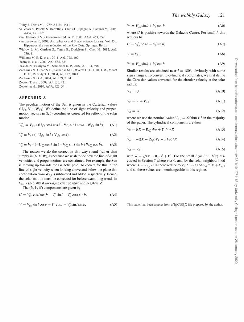
The wobbly Galaxy 121
Tonry J., Davis M., 1979, AJ, 84, 1511Vallenari A., Pasetto S., Bertelli G., Chiosi C., Spagna A., Lattanzi M., 2006,
A&A, 451, 125van Helshoecht V., Groenewegen M. A. T., 2007, A&A, 463, 559van Leeuwen F., 2007, Astrophysics and Space Science Library, Vol. 350,
Hipparcos, the new reduction of the Raw Data. Springer, BerlinWidrow L. M., Gardner S., Yanny B., Dodelson S., Chen H., 2012, ApJ,
750, 41Williams M. E. K. et al., 2011, ApJ, 728, 102Yanny B. et al., 2003, ApJ, 588, 824Yasuda N., Fukugita M., Schneider D. P., 2007, AJ, 134, 698Zacharias N., Urban S. E., Zacharias M. I., Wycoff G. L., Hall D. M., Monet
D. G., Rafferty T. J., 2004, AJ, 127, 3043Zacharias N. et al., 2004, AJ, 139, 2184Zwitter T. et al., 2008, AJ, 136, 421Zwitter et al., 2010, A&A, 522, 54
APPENDIX A
The peculiar motion of the Sun is given in the Cartesian values(U�, V�, W�). We define the line-of-sight velocity and proper-motion vectors in (l, b) coordinates corrected for reflex of the solarmotion:
V ′los = Vlos+(U� cos l cos b+V� sin l cos b+W� sin b), (A1)
V ′l = Vl +(−U� sin l+V� cos l), (A2)
V ′b = Vb+(−U� cos l sin b−V� sin l sin b+W� cos b). (A3)
The reason we do the correction this way round (rather thansimply in (U, V, W)) is because we wish to see how the line-of-sightvelocities and proper motions are constituted. For example, the Sunis moving up towards the Galactic pole. To correct for this in theline-of-sight velocity when looking above and below the plane thiscontribution from W� is subtracted and added, respectively. Hence,the solar motion must be corrected for before examining trends inVlos, especially if averaging over positive and negative Z.
The (U, V, W) components are given by
U = V ′los cos l cos b − V ′
l sin l − V ′b cos l sin b, (A4)
V = V ′los sin l cos b + V ′
l cos l − V ′b sin l sin b, (A5)
W = V ′los sin b + V ′
b cos b, (A6)
where U is positive towards the Galactic Centre. For small l, thisreduces to
U = V ′los cos b − V ′
b sin b, (A7)
V = V ′l , (A8)
W = V ′los sin b + V ′
b cos b. (A9)
Similar results are obtained near l = 180◦, obviously with somesign changes. To convert to cylindrical coordinates, we first definethe Cartesian values corrected for the circular velocity at the solarradius:
VX = U (A10)
VY = V + Vc,0 (A11)
VZ = W, (A12)
where we use the nominal value Vc, 0 = 220 km s−1 in the majorityof this paper. The cylindrical components are then
VR = ((X − R�)VX + YVY )/R (A13)
Vφ = −((X − R�)VY − YVX)/R (A14)
VZ = VZ, (A15)
with R = √(X − R�)2 + Y 2. For the small l (or l ∼ 180◦) dis-
cussed in Section 7 where y � 0, and for the solar neighbourhoodwhere X − R� < 0, these reduce to VR � −U and Vφ � V + Vc, 0
and so these values are interchangeable in this regime.
This paper has been typeset from a TEX/LATEX file prepared by the author.
Dow
nloaded from https://academ
ic.oup.com/m
nras/article-abstract/436/1/101/971163 by University C
ollege London user on 28 January 2020