jupiter s-bursts: narrow-band origin of microsecond subpulses

Jupiter S-bursts: Narrow-band origin of microsecond subpulses

V. B. Ryabov,1,2 B. P. Ryabov,2 D. M. Vavriv,2 P. Zarka,3 R. Kozhin,2 V. V. Vinogradov,2

and V. A. Shevchenko2

Received 23 June 2007; accepted 29 June 2007; published 8 September 2007.

[1] We analyze the records of Jupiter’s decameter radio emissions obtained during an Io-AS-burst storm on 15 March 2005. The observations were performed at the world’s largestdecameter array, UTR-2, which is equipped with a digital receiver capable ofcatching waveforms of duration �3 s with temporal resolution defined by the samplingrate of �66 MHz. A Hilbert transform based algorithm has been applied to study narrow-band spectral patterns demonstrating quasi-linear drift over time-frequency plane. Theinstantaneous amplitude and phase information has been extracted from the recordedwaveforms with the purpose of analyzing microsecond-scale coherent events in the S-burstemission. A statistical model of narrow band random process is proposed fordescribing such features in the observed waveforms as coherent segments, phase jumps,nonlinear frequency drift, etc. It is shown that the study of coherence properties in terms ofinstantaneous phase is equivalent to Fourier analysis of a narrowband signal. Thisimplies that no particular mechanism (such as superimposed modulation or oscillation) isrequired for generating the observed coherent phase structures of S-burst emission: those,as well as the pulse-like envelope structures, emerge naturally at the output of anarrow band filter applied to a random noise. It is further suggested that probabilitydistribution function of instantaneous amplitude gives an important insight into theunderlying physical mechanism of S-burst generation. In particular, it is demonstrated thatmodels based on the concept of ‘‘generator,’’ i.e., a nonlinear system with feedback, areless suitable for reproducing the observational characteristics of S-bursts atmicrosecond time scale resolution. On the other hand, the concept of ‘‘amplifier,’’ i.e., alinear system (without feedback) that enhances the fluctuations within a narrow band, fitsthe observational data well. This conclusion is consistent with S-burst generationmechanism via cyclotron-maser instability, which is indeed a resonant wave amplificationprocess.

Citation: Ryabov, V. B., B. P. Ryabov, D. M. Vavriv, P. Zarka, R. Kozhin, V. V. Vinogradov, and V. A. Shevchenko (2007), Jupiter

S-bursts: Narrow-band origin of microsecond subpulses, J. Geophys. Res., 112, A09206, doi:10.1029/2007JA012607.

1. Introduction

[2] The details of how decameter radio bursts are gener-ated in the magnetosphere of Jupiter are still a matter ofdebate. From a macroscopic viewpoint, the bursts aremainly produced in the electric current system caused bythe electromagnetic interaction of Jupiter with its closestGalilean moon Io (Io flux tube (IFT)). The motion of themoon through the Jovian magnetic field results in a�400 KVpotential drop across Io [Goldreich and Lynden-Bell, 1969;Saur et al., 2004] and hence the conditions for acceleratingelectrons are created in Io’s vicinity. On a microscopic scale,when the motion of a test particle is analyzed to predict theobserved properties of radio emissions, one possible scenario

[Ellis, 1965; Zarka et al., 1996] considers non relativistic(<10 KeV) electrons, which accelerate near Io and moveadiabatically towards the planet along Jovian magnetic fieldlines. They are then reflected back from mirror pointslocated at different altitudes defined by both the strengthof the magnetic field and the electron initial pitch angles[Galopeau et al., 1999]. The electrons able to penetratedeeply into the atmosphere are lost due to collisions withambient atmospheric atoms and molecules (producing a UVaurora), whereas those reflected at high enough altitudesstart the backward motion toward Io. As a result of such‘‘selective mirroring,’’ initially Maxwellian distribution ofelectron velocities in the downstream current is transformedto an empty-loss-cone distribution in the upward streamslightly above the mirror points. Such distributions canamplify electromagnetic waves via the cyclotron masermechanism [Wu and Lee, 1979], if the frequencies of thepropagating waves are in resonance with gyrating electrons.[3] Theories based on the qualitative picture given above

can successfully interpret many observational features of

JOURNAL OF GEOPHYSICAL RESEARCH, VOL. 112, A09206, doi:10.1029/2007JA012607, 2007ClickHere

for

FullArticle

1Future University-Hakodate, Hakodate, Japan.2Institute of Radio Astronomy, Kharkov, Ukraine.3Laboratoire d’Etudes Spatiales et d’Instrumentation en Astrophysique

LESIA, Paris Observatory, Meudon, France.

Copyright 2007 by the American Geophysical Union.0148-0227/07/2007JA012607$09.00

A09206 1 of 20

http://dx.doi.org/10.1029/2007JA012607

Jupiter’s decameter radio emissions, such as, e.g., a hollowcone geometry of radio waves beaming [see, e.g., Zarka,1998], high brightness temperature of the radio source,upper cutoff frequency at about 40 MHz as well as thelower one at about 1.5 MHz [Zarka et al., 2001], prevailingnegative frequency drift on the time-frequency plane,polarization properties of radiation, etc. However, themechanism responsible for pulse-type emissions duringthe so-called S-burst storms, when the most powerful spikescharacterized by fast frequency drift are generated, remainsunclear. The ‘‘S’’ in ‘‘S-bursts’’ stands for ‘‘short’’ toaccount for typical pulse durations of several tens of milli-seconds and to be distinguished from L-type emissions(‘‘L’’ means ‘‘long’’) characterized by timescales of theorder of several seconds [Carr et al., 1983]. Variousapproaches aimed at explaining the generation mechanismof complex time frequency patterns observed during S-burststorms have been proposed. Several, such as chain reactionof elementary ruptures of current filaments [Ryabov, 1994]or coherent emission produced by the phase bunchingmechanism [Willes, 2002], look promising for elucidatingthe observed complexity, but no theory can explain all theobservational facts as a whole. Example spectrograms ofJupiter radio emission during a typical S-burst storm aregiven in Figure 1. Figure 1b presents comparatively simpletime-frequency patterns, when almost linear frequency driftsof individual S-bursts are produced, whereas Figure 1aprovides an example of more complex structures thatcontain spectral patterns with highly variable frequencydrift rates. It should be also noted that complex S-burstspectrograms, like those shown in Figure 1a or likewise,typically occur more often than those exemplified inFigure 1b [Boudjada et al., 1995; Ryabov et al., 1997]. Asa rule, they are observed in themiddle part of a typical S-burststorm lasting about 1 to 1.5 hours [Ryabov et al., 1997],whereas simple ones appear at its initial (first 5–10 min.)and final (last 10–15 min) stages.[4] In order to elucidate the physical mechanism respon-

sible for generation of ‘‘simple’’ S-bursts it seems necessaryto increase the temporal resolution and look at the S-burstsignal on a microsecond timescale. Using a baseband re-ceiver with a half-voltage bandwidth of the order of 280 kHzcombined with a tape recorder and data rate slow downtechnique, Carr and Reyes [1999] achieved a sampling rateequivalent to about 0.3 ms. The most important findingsfrom earlier works can be roughly summarized as follows[Carr and Reyes, 1999; Carr, 2001; Litvinenko et al., 2004].[5] 1. The envelope (or time-dependent amplitude) of

simple S-bursts reveals fluctuations with characteristic timescales within the range of 50–190 ms. Hereinafter, thosefluctuations will be referred to as ‘‘subpulses.’’[6] 2. Some (actually, few ones in any separate S-burst)

of the subpulses are coherent, i.e., can be well approximatedby sinusoidal functions of fixed frequency and initial phase.[7] 3. The detectability of coherent subpulses in an S-burst

depends on the signal-to-noise ratio, i.e., on the instanta-neous value of the signal amplitude (if we assume approx-imate stationarity of the experimental noise coming fromcosmic background + technical fluctuations in the registeringequipment).[8] 4. The instantaneous phase (measured over the inter-

val of length �3 ms) demonstrates characteristic phase

jumps, i.e. sudden changes in the phase value, at momentswhen the signal-to-noise ratio is close to zero. The value ofthe phase change is sometimes close to 180�, thus beinginterpreted as ‘‘phase reversals.’’[9] 5. It has been concluded that the mechanism of S-burst

generation may consist in successive subbursts from coher-ent structures located at different altitudes in the Io-Jupiterelectric current system. The observed frequency drift istherefore defined by the speed of propagation of theemission triggering process through the electron stream(see also similar scenario discussed in detail in the workof Ryabov [1994]).[10] Currently, a number of fundamental questions

concerning the analysis of S-burst signals with microsecondtime resolution remain open. In particular, the main assump-tion on the possibility of detecting qualitatively new infor-mation by drastic increase in temporal resolution seems tocontradict the fundamentals of Fourier analysis. Indeed, therelation of Df � Dt � 1 establishes a restriction on theinstantaneous frequency band Df of any time-frequencypattern defined by the temporal resolution Dt used in theanalysis. Therefore any significant increase in time resolu-tion controlled byDtmay bring uncertainty in the frequencydomain and result in overall loss of information andincreased noise level.[11] The purpose of this paper is to develop a quantitative

framework for the analysis of coherence properties of S-burstemission and propose a prototype mathematical model thatcan reproduce the S-burst waveforms. Contrary to the ideasreported by Carr and Reyes [1999], who focused onmodeling subpulses as segments of sinusoidal functions(e.g., generated by coherent bunches of electrons movingalong Jovian magnetic field lines), we consider the basicmodel of Gaussian noise enhanced by a narrow-bandresonance amplifier (maser).[12] The proposed mathematical description is applied to

the analysis of Jupiter S-bursts recorded at the world’slargest decameter radio telescope, UTR-2, equipped with adigital waveform recorder. First, we analyze the instanta-neous amplitude and phase of S-bursts by applying theconcept of analytic signal based on Hilbert transform[Tikhonov, 1986] directly to the recorded baseband timeseries. This enabled us, on one hand, to confirm thepresence of amplitude fluctuations (subpulses) on a micro-second timescale, and, on the other hand, to develop newmethods of detecting the coherent segments in the data asphase invariant intervals in instantaneous phase temporalprofiles. Second, we utilize a statistical theory of narrow-band Gaussian random processes for obtaining estimates ofexpected values of phase, amplitude, and their variances.Such an approach provides an explanation for rapid changesin the phase time behavior known as ‘‘phase jumps’’ [Carr,2001]. We show that they appear as a result of enhancedphase fluctuations caused by the geometric property of thepolar coordinate system near the origin. Finally, we discusstest models for distinguishing two physically relevant casesof narrow band amplitude fluctuations in S-burst wave-forms: (1) fluctuations in a weakly nonlinear van der Pol-type oscillator (generator) and (2) noise passed through anarrow-band linear filter (resonance amplifier). The analysisof the distribution function of amplitude fluctuations leadsto the conclusion of more probable amplifier mechanism

A09206 RYABOV ET AL.: JUPITER S-BURSTS

2 of 20

A09206

responsible for producing the S-burst emission rather than aself-sustained generator-type instability.

2. Observations and Equipment

[13] Since 2004, a new digital receiver system DRATFA(Decameter Radio Astronomy Time-Frequency Analyzer)has been developed, tested, and installed at the UTR-2decameter array [Braude et al., 1978] located near Kharkovcity, Ukraine. In addition to real-time Fourier-analysis, thesystem allows direct baseband recording with a samplingfrequency of �66 MHz at 16 bits precision, which providesan opportunity for analyzing signals within the band of 0 !33 MHz without frequency down-conversion.[14] It should be noted, however, that in order to avoid

signal pollution by powerful in-band man-made interferencesignals from terrestrial broadcasting stations, communica-tion transmitters, etc., we had to restrict the observationalband and utilize analog pass-band filtering with cut-offfrequencies of 15 and 30 MHz at the input of our receiver

system. The lower cut-off frequency was selected above thefrequency of the most powerful interference, around thelocal minimum of S-burst occurrence probability [seeRyabov, 1994, Figure 6b]. This did not encroach uponindividual S-bursts in the nearest occurrence subband locatedaround the frequency of �16.5 MHz. The upper cutofffrequency was defined by the decline of frequency responsefunction of the UTR-2 array above 30 MHz.[15] Note that such combination of characteristics in the

utilized equipment as high sensitivity of the antenna array(world’s largest decameter telescope), with the workingbandwidth of 8–32 MHz and source tracking time of�8 hours, waveform analyzer for baseband direct recordingof �3 s continuous data segments to the hard disk ofcomputer, and high-capacity digital storage system capableof efficient manipulation, display, and processing of severalhundreds of Gigabytes of experimental data, represents aunique observational system that, up to our knowledge, hasnot been reported elsewhere.

Figure 1. Fragment of the Io-A S-burst storm of 14 March 2005. (a) Dynamic spectra for complexS-bursts and (b) comparatively simple linearly drifting S-burst patterns recorded about 22 min earlier. Thespectrograms were calculated by applying a windowed Fourier transform to observational data sampled at�66 MHz. Owing to high pass filtering applied for enhancing the contrast of S-burst patterns, the L-burststorm below 23.5 MHz that accompanies the S-bursts seen in the spectrogram (Figure 1b) is not clearlyvisible.


3 of 20

A09206

Figure 2. (a) A fragment of the S-burst spectrogram presenting the selected for the analysis linearlydrifting pulse of emission. The white arrow indicates the position of the inflection point, where thelinearity of the frequency drift is broken (see also Figure 11). (b) An enlargement of the fragmentpresented in Figure 2a. The intermittent bright line at about 24.7 MHz demonstrates amplitudefluctuations. (c) The instantaneous amplitude of the signal shown in Figure 2b is calculated by applying aHilbert transform to the time series and constructing the analytic signal. The beginning of Figure 2ccoincides with that of Figure 2b and Figure 1b.


4 of 20

A09206

[16] The observations were performed on 14 March 2005,between about 0130 and 0230 UT, during a powerful Io-AS-burst storm. After passing through the analog bandpassfilter, the signal from the UTR-2 array was digitized at a66 MHz rate and then transferred to the RAM of the hostPC. After filling up the RAM memory buffer, the dataacquisition process was interrupted to save the data to thedisk. This procedure resulted in about 3 s continuous datasegments (defined by the size of 1 GB RAM memory ofutilized host PC) separated by approximately 12 s pausesrequired to save the data to the hard disk. Despite thefragmentary character of the recordings, the amount of datacontaining S-burst signals clean from interference wassufficient for further analysis. The total duration of therecorded S-bursts was about 900 s, i.e., the number ofindividual pulses can be estimated as �104 in the continu-ous band of 15 MHz.[17] As a starting point of our data processing, we select

the data segment shown in the bottom panel of Figure 1where the S-bursts demonstrate a comparatively simplepattern of quasi-linear frequency drift. All individual simpleS-bursts look similar at the microsecond time resolution;therefore we can take a single frequency drifting pulse as anobject for our study and analyze its instantaneous phase andamplitude by applying a Hilbert transformation and buildingthe analytic signal (described in Appendix A). Successiveenlargements of the selected burst down to the scale wheremicrosecond subpulses become evident are shown inFigures 2a and 2b. The subpulses with characteristic period�100 ms can be easily identified in Figure 2b as maxima ofcolor intensity in the intermittent bright line clearly visibleat about 24.7 MHz. We also show in Figure 2c the timeprofile of the subpulses amplitude corresponding to Figure 2b.It is, in fact, the profile of instantaneous amplitude of theanalytic signal reconstructed by using the Hilbert transformprocedure.

3. Signal Preprocessing and Hilbert Transform

[18] The idea of coherence, originally introduced in thefield of optics [e.g., Goodman, 1968], refers to the propertyof a wave to preserve its sinusoidal shape with time and/orin space. Such an approach implicitly assumes a harmonicoscillation as an adequate mathematical model that has to befitted to the measured time series. Carr and Reyes [1999]proposed a short segment of harmonic signal

S tð Þ ¼ sin

cos2pft þ d0ð Þ;

called a ‘‘local oscillator voltage’’, to be used as a basicmodel, correlated with the recorded S-burst voltage v(t) in ashort time interval (50–200 ms). They calculated acorrelation coefficient between the two signals, S(t) andv(t), applied a fitting procedure for finding parameter valuesof frequency f and phase d0 for the harmonic signal, and,finally, extracted the phase information from simpletrigonometric arguments. We, however, found certainlimitations in this approach, namely, (1) it does not takeinto account the background noise fluctuations, which playan important role in the temporal phase dynamics (seebelow) and (2) several implicit parameters (e.g., a time

constant of smoothing filters) used in the best-fittingprocedure are not clearly defined and require furtherjustification.[19] In order to avoid the technical difficulties men-

tioned above, and considering the instantaneous narrowband of S-bursts, we accept a generalized concept of‘‘narrow band random process’’ (hereinafter, NBRP) widelyused in statistical signal processing literature [Rice, 1945;Levin, 1969; Tikhonov, 1986] as our working model. Inaddition to the advantage of using the many theoreticalresults available for this class of signals, it allows efficientalgorithms based on the Hilbert transform to be used for adirect evaluation of instantaneous values of amplitude,phase, and frequency (see Appendix A).[20] It should be noted that NBRP was initially intro-

duced as a mathematical model of signals having narrowbandwidth Df around some ‘‘central’’ frequency f0 locatedfar from zero, so that the condition f0 � Df had to besatisfied. In particular, this model allowed efficient analysisof the effect of passing the signal through the input filters ofrecording equipment (e.g., through the intermediate fre-quency filter of a typical receiver), as well as to studyvarious transformations the signal further undergoes intypical receiver circuits, e.g., a frequency mixer, squaredetector, and low-pass filter. In addition, noise character-istics of the signal at every stage of such a transformationcan be studied in detail.[21] Although in our observations the recorded signal was

wideband (Df = 15 MHz, f0 = 22.5 MHz), we had totransform it to a NBRP type at the initial stage of ouranalysis. This was stipulated by the necessity of separating asingle S-burst from man-made terrestrial interference sig-nals and other emissions from Jupiter present in the workingband simultaneously with the analyzed pulse. The digitalnarrow-band filter that we introduce at the input of oursignal processing procedure has a much larger bandwidththan the instantaneous frequency range occupied by theanalyzed S-burst, but is much smaller than its centralfrequency. Throughout almost all the calculations reportedin this paper we used the filter of bandwidth Df = 0.5 MHzlocated at some (varied) central frequency within theinterval of 23–27 MHz.

4. Signal Plus Noise at the Output of aNarrow-Band Filter

[22] Before starting our analysis, we note that the signalwe obtain at the input of the Hilbert transform actuallyconsists of two parts: (1) NBRP(1) with a typical bandwidthof �0.5 MHz defined by input (digital) filter and (2) anotherNBRP(2) of considerably smaller bandwidth that corre-sponds to a frequency drifting S-burst signal. The inputfilter efficiently cuts out the components not related to thechosen S-burst emission pattern from the dynamic spec-trum. The time-frequency components that occur simulta-neously with the S-burst pulse of emission selected for ouranalysis are clearly seen on the spectrogram in the bottompanel of Figure 1. In our data time window that approxi-mately corresponds to the first 8 ms of the spectrogramshown in Figure 1b, another S-burst spectral pattern (at about25.8 MHz) and a wide-band L-burst emission (at about23 MHz) characterized by a slowly varying amplitude


5 of 20

A09206

envelope are observed together with the analyzed S-burst(located at about 24.7 MHz). A typical average powerspectrum of the data segment we analyze that contains allthe components mentioned above is depicted in Figure 3a,whereas in Figure 3b and 3c, we show the spectrum ofa NBRP obtained from the original signal passed through a0.5 MHz band-pass input filter. The S-burst signal forms a�150 kHz peak in the spectrum seen in Figure 3c. Note thatthe bandwidth of the depicted S-burst component is muchwider than the instantaneous S-burst band that constitutes�10–30 kHz (as follows from numerical analysis of spec-trograms shown in Figures 1 and 2). This is a directconsequence of the frequency drift of the S-burst withinthe analysis window of �8 ms duration. A rough value ofthe frequency drift rate can be obtained from the estimatesabove as 150 kHz/8 ms 18 MHz/s. It is also important totake into account that the instantaneous frequency of S-burstemissions typically does not coincide with the centralfrequency of the filter, i.e., there is a time-dependentfrequency mismatch Df between the center of a driftingS-burst and the maximum of the frequency response func-tion of the filter.[23] Clearly, in the NBRP shown in Figures 3b and 3c we

can refer to the signal of the first part as ‘‘noise’’ and secondone as ‘‘signal.’’ Although the signal-to-noise ratio is ratherhigh for the recorded S-burst, the background part cannot beneglected, since it plays a crucial role in the overall patternof temporal phase evolution. In order to demonstrate theimportance of the interplay between the two components ofthe signal, we have to consider two fundamental types ofNBRP described in detail in Appendix B, noise only andsignal plus noise. Heretofore, we shall refer to those types asNBRP of type 1 and 2, correspondingly.[24] In Figure 4 we show examples of the time profile

of NBRP of the first type (Figure 4a) and its amplitude(Figure 4b) for a process of effective bandwidth �0.5 MHz.The signal has been obtained by passing sky backgroundfluctuations through the input filter centered at a frequencylocated far enough from any present S-burst pattern. Thecharacteristic period of envelope variation is defined in thiscase by the inverse of its effective bandwidth and constitutes

Tc ¼1

Df 2 ms:

Note also that any attempt of ‘‘smoothing’’ the variation ofamplitude with, say, a low pass filter with a bandwidth of�10 kHz results in the appearance of an amplitude profile(Figure 4d), which is qualitatively similar to that shown in

Figure 3. (a) Power spectrum of the analyzed signalcalculated at the output of the �15 MHz band pass filterinstalled after the UTR-2 array. The Fourier transform hasbeen performed in a�8 ms time window. L- and S- emissionpeaks are clearly visible. Note also the presence of �5 dBdrop in the frequency response function of the UTR-2antenna system at about 18 MHz. (b) Signal at the output of0.5 MHz filter, a single S-burst emission component isseparated from other signals. (c) Zoomed version of the plotshown in Figure 3b. Central frequency of the filter, notcoinciding with the central frequency of the S-burstcomponent, is indicated by dashed line.


6 of 20

A09206

Figure 2c. The resemblance consists in the presence of‘‘subpulses’’ of approximately same characteristic timescale of �100 ms. Therefore special care is needed todistinguish these fluctuations (caused by the sky back-ground noise) from S-burst subpulses.[25] The NBRP of type 2 discussed in Appendix B is the

sum of two narrow-band noise signals. Although bothcomponents also belong to the class of NBRP, their char-acteristic timescales are significantly different. The typicalinstantaneous bandwidth of the S-burst signal is �10–30 kHz, whereas the utilized pass band of the input filteris �500 kHz. This property enables us to consider theformer as being approximately sinusoidal at the timescalemuch larger than the characteristic period of the latter.Therefore we assume that the following model can be usedfor NBRP of type 2

h tð Þ ¼ x tð Þ þ S tð Þ; ð1Þ

where S(t) =A0(t1)cos(wt +Dwt + f0(t1)) is a quasi-harmonicsignal of amplitude A0(t1), angular frequency w + Dw, andinitial phase f0(t1); t1 = e1t is ‘‘slow’’ time, and e1 1 is asmall dimensionless parameter defined by the ratio of thequasi-harmonic signal bandwidth to the bandwidth of thewider-band background component. If the instantaneousfrequency of the signal S(t) coincides with the centralfrequency of the noise component x(t), the parameter Dwof frequency mismatch vanishes. This condition, however,does not hold in a typical situation encountered in theanalysis of S-bursts, due to the presence of frequency drift.As we show below, the non-stationary frequency detuningof the S-burst with respect to the central frequency of thefilter is one of the causes for ‘‘phase jumps’’ reported earlierby Carr [2001] as a typical feature in the temporal profilesof S-burst phase evolution.

5. Temporal Variation of Phase

[26] When the signal to noise ratio is high, subpulses areclearly visible in amplitude time profiles, as shown, e.g., inFigure 2c. The question of their degree of coherenceremains uncertain, however, and demands further clarifica-tion. It is natural to demand that the property of coherenceshould be associated with phase invariance during coherentevents. In order to make this idea precise and perform aquantitative analysis, an algorithm for extracting phase fromthe available experimental time series is needed. Themethod we selected for this purpose is based on the conceptof analytic signal that is described in detail in Appendix A.The computation procedure includes performing a Hilbert

Figure 4. Narrow-band Gaussian process (noise) at theoutput of input filter of 0.5 MHz bandwidth: (a) the originalsignal; (b) instantaneous amplitude of analytic signal(envelope) demonstrate fluctuations with characteristicperiod of �2 ms; (c) same as Figure 4b but in a longertime interval; (d) spurious low-frequency envelope fluctua-tions caused by the low-pass filtering of the signal shown inFigure 4c with cut-off frequency �10 kHz. The fluctuationamplitude in Figure 4d is reduced compared to Figures 4band 4c due to the effect of filtering.


7 of 20

A09206

transform on the signal obtained after the input filteringwith 0.5 MHz bandwidth, making an analytic signal bycombining the original time series with the transformed onein accordance with equation (A2), and calculating the fullphase Y(t) = wt + c(t) by formulas (A4).[27] At the next step of analysis, we calculate the time

dependent function c(t) that describes temporal dynamics ofphase in the reference frame rotating at some predefinedangular frequency wr. Owing to the presence of frequencydrift in S-burst signal, the choice of the value of wr issomewhat arbitrary and can be made based on the criterionof approximate stationarity of frequency within the analysistime window (see below). An example of phase temporalprofile for an S-burst segment is shown in Figure 5a. In thisplot, the value of wr has been chosen to be equal to thecentral frequency of the input filter. Apparently, linearlygrowing intervals corresponding to subpulses can be easilyidentified by visual inspection of this plot, and the growthrate is defined by the frequency mismatch between wr andthe instantaneous frequency of the S-burst segment.[28] Although the algorithm for extracting the full phase

Y(t) from the experimental time series is straightforward, thenext step of identifying stationary segments corresponding tosubpulses can be a nontrivial task. Finding phase coherentintervals requires the detection of approximately constant-phase-segments in the ‘‘slow’’ phase profiles c(t) = Y(t) �wrt at a suitably chosen value of the ‘‘fast’’ frequency wr.However, owing to the presence of frequency drift, thevalue of wr changes with time; therefore the condition ofphase constancy can be satisfied only within comparativelyshort time intervals. Therefore for each of the detectedsubpulses, we have to define a time interval of durationT0, in which approximate invariance of frequency can beassumed. A condition for selecting the length T0 of such atime window can be suggested, e.g., from the requirementthat phase deviation induced by the frequency drift wouldbe not greater than �2p. In our example S-burst shown inFigure 2, the average linear frequency drift measured by linearfit to the positions of maxima in spectral power profilesconstitutes about �17 MHz/s. This corresponds to a phase

Figure 5. Instantaneous phase c(t) = Y(t) � wrt of theS-burst signal corresponding to (part of) the fragment shownin Figures 2b and 2c. The central frequency of the inputfilter (�0.5 MHz bandwidth) has been chosen the same asthat of wr = 2pfr; fr = 24.65 MHz. Linearly growing phaseintervals that exist due to a non-zero frequency mismatchDf between the instantaneous frequency of the S-burst andfr are interrupted by irregular phase variation intervalscorresponding to phase jumps. (b) Instantaneous phase aftersubtracting the linearly growing term from the fragment shownin Figure 5a, i.e. changing the value of fr to 24.71 MHz.Subpulses are now clearly identified as intervals of quasi-stationary phase between apparent phase jumps. (c) Low-pass filtered (filter time constant is �30 ms) fragment of thetime profile of instantaneous amplitude corresponding toFigure 5b. Position of subpulses coincides with the intervalsof high amplitude. (d) Same as Figure 5c but calculated withhigher cut-off frequency of the low-pass filter (time constant�4 ms). Shorter subpulse at about t = 2.17 ms can now beseen in the amplitude profile.


8 of 20

A09206

deviation of �2p within a time interval of �500 ms. InFigures 5b–5d we plot a stationary segment of duration�500 ms located around one of the subpulses shown inFigure 2c. One can associate the subpulses with apparentplateaus in Figure 5b that occur simultaneously with highamplitude values shown in Figure 5c. The third (from theleft) phase-invariant segment does not correspond to anamplitude pulse in Figure 5c due to smoothing that weapplied to the amplitude curve. In Figure 5d we plot thesame amplitude profile as that shown in Figure 5c, but with amuch smaller time constant of the smoothing filter. Smallpulse of instantaneous amplitude becomes evident at aboutt = 2.17 ms.[29] The value of the ‘‘reference’’ frequency wr in the

segment shown in Figure 5b has been set at �24.71 MHz,whereas the input filter (�0.5 MHz bandwidth) has beentuned to the same central frequency as in Figure 5a, i.e., fc =24.65 MHz. As discussed in Appendix B, such settingsinduce phase jumps caused by switching between the two

frequency components which are separated by about Df 0.06 MHz, as can be clearly seen in Figure 5b. In otherwords, the stationary phase segments are interrupted by theintervals of fast phase drift where the phase changes at arate of �0.4 rad/ms (a close estimate can be also obtainedfrom the average slope of the drifting phase segments inFigure 5b).[30] We therefore conclude that (at least some of) the

‘‘phase jumps’’ (initially discussed by Carr [2001]) couldbe interpreted as a manifestation of an existing frequencydifferenceDf between the instantaneous frequency of S-burstand central frequency of the input filter. As soon as thepower of an S-burst becomes low, the measured phase of therecorded signal starts rotating at the rate of Dw = 2pDf thatlooks like a ‘‘phase jump’’ in the temporal profile of the‘‘slow’’ phase. If Df = 0, the task of identifying separatesubpulses in the phase temporal profiles becomes compli-cated, because the only feature that distinguishes coherentsegments from noncoherent ones becomes the variance ofthe instantaneous phase. The segments corresponding tohigh amplitudes are thus characterized by low varianceoscillations, whereas those at small amplitudes look more‘‘noisy.’’[31] It should be noted, however, that nonzero frequency

mismatch is not the only mechanism that can produce the‘‘phase jumps’’ observed in the phase temporal profiles.Even at vanishing frequency mismatch, i.e., if Df 0, thecalculated value of phase can demonstrate the phase jumpsby �2pn rad, where n is an integer number. This phenom-enon can be explained by the extreme sensitivity of phase tofluctuations, when the value of instantaneous amplitudeapproaches zero [Moe and McArtor, 1965]. The noise-induced wandering of the tip of the vector r(t) (seeFigure 6) may cause random phase slips of magnitude2p every time the tip approaches the origin close enough.The fact that such jumps always appear as 2p -multiplesoccurring if (and only if) the corresponding instantaneousamplitude value is low means that such jumps are merelydefined by the noise component x(t) and are not related tothe physical processes responsible for the S-burst signalS(t). A demonstration supporting the hypothesis on twodifferent mechanisms leading to phase jumps is depicted inFigure 7, where we plot the same data segment as shown inFigure 5, but calculated with the input filter centered at�24.71 MHz and a bandwidth of 0.1 MHz. The four curvesshown in Figure 7 are, in fact, one profile (the heavy line inFigure 7), but shifted by a value of 2p. A comparison withFigure 5b reveals that the first two phase jumps located atabout t 1.96 ms and t 2.15 ms disappear in Figure 7;therefore their presence in Figure 5b can be attributed to thefiltering effect with the nonzero frequency mismatch. Thesubsequent phase jump located at t 2.2 ms in Figure 5bremains in Figure 7, although its magnitude is reduced.Therefore the latter can be interpreted as the combinedeffect of both the frequency mismatch and noise. Note thatthe remaining jump amplitude in Figure 7 is a 2p -multipleas illustrated by plotting several phase temporal profilesshifted by 2p. The phase calculated by modulus 2p appearsconstrained between the two dashed lines thus demonstrat-ing the absence of S-burst signal phase jumps between thesubpulses. Taking into account the low value of instanta-neous amplitude corresponding to the jump location (see

Figure 6. (a) Vector diagram – geometric interpretation ofnarrow-band Gaussian process x(t) of amplitude A(t) andphase y(t). (b) Same diagram for the sum of narrow-bandGaussian process x(t) of amplitude A(t) and a quasi-harmonic signal S(t) with amplitude A0(t). The resultingsignal h(t) is also narrow-band Gaussian process withamplitude r(t) and phase c(t).


9 of 20

A09206

Figure 5c), as well as close to zero frequency mismatch, onecan conclude that random wandering of the signal in thevicinity of the origin is the main cause of this jump event.[32] Although the phenomenon of phase jumps does

not seem to provide physical information on the processof S-burst generation, it still can be utilized in a constructiveway for developing a computer algorithm for the automaticdetection of subpulses. The algorithm we realized consistsin building a histogram of instantaneous phase values inevery window of approximate frequency stationarity oflength T0, at a nonvanishing value of the frequency mis-match (Dw 6¼ 0). In Figure 8, we show a histogramcorresponding to the phase plot shown in Figure 5b. Thesubpulses correspond to peaks in such histograms due to thecomparatively small phase variance when the instantaneousamplitude is high, and rapid phase rotation accompanyingthe low amplitude values. The procedure for choosing asuitable threshold value in the histogram, as well as thesearch for the optimal frequency wr and identification oftime-continuous segments of stationary phase corres-ponding to peaks in histograms have been developed.[33] After compiling a sufficiently long list of subpulses

from the S-burst selected for our analysis, we performedseveral tests aimed at quantifying their coherence properties.At first, we tried to clarify whether the phase is preservedbetween two successive subpulses, i.e., we searched for thepresence of a long time memory in S-bursts. Our study ofseveral S-burst records revealed no significant correlationbetween the average phase of successive subpulses. InFigure 9 we plot a scatter diagram illustrating this fact,i.e., for a set of numerically detected subpulses, the averagephase of each subpulse is plotted against that of the

subsequent subpulse. In terms of Figure 5b, this graphcorresponds to plotting the phase averages calculated overtwo successive plateaus separated by a phase jump. Figure 9demonstrates the absence of correlated values betweenabscissa and ordinate, as evidenced by the appearance ofno point clustering. This means that although each subpulsecan be well approximated by a pure harmonic signalsomewhat corrupted by noise, its initial (or average) phaseis random.[34] The scattering of phases between subpulses in a

narrow band process can be interpreted in various ways.For example, the subpulses can be produced by a maseramplifying the background fluctuations, and the observednarrow bandwidth is defined by the resonance character ofthe amplification process. Another interpretation could bethe fluctuations in an oscillatory system controlled by arandom process. In such a case, the system can generatepulses, each of which is coherent, but initial phase israndom. One more possibility is that randomness is imposeddue to the complex spatial shape of a coherent source in theIo flux tube, resulting in random phases of received radia-tion caused by the propagation effect.[35] Another characteristic that could be suggested as a

test for the presence of coherence in subpulses is theamplitude of fluctuations in the instantaneous phase aroundthe mean value within a single subpulse. It should be notedthat the variance of phase in a NBRP consisting of a mixtureof purely harmonic signal with narrow-band Gaussian noiseis defined by equation (B7). As follows from (B7), its phasevariance is merely defined by the amplitude of harmoniccomponent. The variance is maximal (=p2/3) if the harmon-ic component is absent and decreases as the instantaneousamplitude of the signal grows. The behavior of phasevariance calculated for the ensemble of numerically foundS-burst subpulses corresponds well with the above scenario.We superimpose on Figure 10 the open circles correspondingto the calculated standard deviation of instantaneous phase

Figure 7. Same as Figure 5b, but at zero frequencymismatch Df between the instantaneous frequency of theS-burst and the central frequency of the input filter. Thebandwidth of the input filter has been also changed to0.1 MHz. Phase fluctuations during time intervals corre-sponding to low values of instantaneous amplitude make theidentification of subpulses problematic. Four curves corre-spond to the same phase temporal profile (heavy) shifted upby 2p. Two horizontal dashed lines mark the interval wherethe phase (mod 2p) can be considered unchanged.

Figure 8. Histogram of instantaneous phase for the plotshown in Figure 5b. Peaks correspond to the segments ofapproximate phase stationarity. The horizontal line showsan empirically chosen threshold separating the peak valuesfrom the rest of the histogram.


10 of 20

A09206

for a set of subpulses detected numerically. The line in thesame plot shows the ‘‘theoretical’’ value calculated byequation (B7). One can observe a good fit between theexperimental data and the values predicted by the statisticalmodel. This means that the phase variance is fully con-trolled by the amplitude of the signal present in the analyzedfragment, and no abnormally ‘‘ultracoherent’’ subpulse ofextraordinarily small dispersion can be found.

6. Time Dependence of Frequency

[36] The nonstationarity of phase leading to phase jumpsdiscussed in the previous section can also be illustrated bythe analysis of the instantaneous frequency wi of the S-burstsignal. It is usually assumed [Ellis, 1965; Zarka et al., 1996;Hess et al., 2007] that adiabatic motion of electrons alongIFT approximately corresponds to linearly drifting S-burstpatterns across the time-frequency plane. The drift rate mayexperience slow changes but can be considered approxi-mately constant within a frequency band of, say,Df = 1MHz.Nonmonotonous deviations from linearity can be associatedwith perturbation of the magnetic field [Dessler and Hill,1979; Ryabov, 1994], particle acceleration or decelerationprocesses, and thus provide important clues to understand-ing the fine structures of plasma in the IFT as well as thephysics of potential drops, parallel electric fields, and othernonlinear effects [Galopeau et al., 1999; Hess et al., 2007].Therefore it appears important to consider the frequencyvariation in addition to the study of the phase dynamicsperformed in the previous section.[37] Similar to the ‘‘phase approach’’ to the analysis

of subpulses described above, the coherent segmentscorresponding to quasi-stationary phase intervals can beidentified in terms of frequency as approximately constant-value intervals. Each subpulse is characterized by its meanfrequency, which varies due to both the presence of fre-quency drift and natural fluctuations. In Figure 11a, we plot

the time evolution of average frequencies of subpulses,calculated by a linear fitting procedure to the full phasetemporal variation curve (like that shown in Figure 5a)within each subpulse taken separately. Every point on thisdiagram corresponds to a segment of quasi-stationary phasebetween two adjacent phase jumps found by the histogramanalysis described above. Fluctuations lead to scattering ofpoints around an approximately linearly drifting pattern withan average slope of about �15.5 MHz/s. In Figure 11b weplot the residuals of the plot shown in Figure 11a obtainedafter subtracting the average linear trend. It is interesting tonote that the frequency drift rate can be considered approx-imately constant within the first half of the analyzed

Figure 9. Average phases (mod 2p) of 664 successivesubpulses for a segment of S-burst of about 30 ms durationbefore the inflection point (see Figures 2 and 11). Absenceof apparent clustering demonstrates an absence of long-timephase correlations.

Figure 10. (a) Mathematical expectation for the instanta-neous amplitude r of the sum of harmonic signal withamplitude A0 and narrow-band Gaussian process withstandard deviation s calculated by formula (B6).(b) Standard deviation for the instantaneous phase c,depending on the amplitude A0 of harmonic component,according to equation (B7). The open circles correspond tos -values obtained by numerical analysis of subpulses in theanalyzed S-burst fragment.


11 of 20

A09206

fragment, but experiences significant deviations from linearbehavior starting at about t = 30 ms. The change in the driftrate can be also noticed in Figure 2a, where one can observea deflection point marked with a white arrow. Thosefluctuations with characteristic time scale of several tensof milliseconds may correspond to local perturbations in themagnetic field.[38] On the other hand, it is possible to estimate the

instantaneous frequency value from the definition of fre-quency as a time derivative of the full phase

wi ¼ 2pfi ¼dY tð Þdt

ð2Þ

In order to get further insight to its variation within asubpulse, we performed the frequency analysis with a muchfiner time resolution by differentiating the time series of thefull phase found from analytic signal in accordance withequation (2). It should be noted, however, that the directcalculation of frequency by applying formula (2) leads tosignificant fluctuations due to the noise amplificationproperty of any differentiation operator, as well as to anunlimited value of variance that can be expected for theinstantaneous frequency [Moe and McArtor, 1965]. For thepurpose of making evident the quasi-constant frequencysegments, we applied a low-pass filtering with a character-

istic time constant of �30 ms after the differentiationprocedure. The result is shown in Figure 12, where we plota segment of analyzed S-burst (Figures 12a and 12b), and itszoomed fragment (Figure 12c) demonstrating an approx-imate frequency invariance during each of the subpulses.For the matter of comparison with the results of the phasestudy given above, we selected an analysis windowoverlapping with that depicted in Figure 5. Note that thesubpulse locations that appear as plateaus on both pictures(Figures 5b and 12c) almost coincide, but fluctuations aremore pronounced on the latter due to infinite variance of theinstantaneous frequency estimate.[39] In Figures 12b and 12c, we also draw the line of the

best fit corresponding to the average negative frequencydrift rate of about �17.4 MHz/s for the given fragment ofthe S-burst, as well as the horizontal line corresponding tothe central frequency of the input filter at 24.65 MHz.Coherent subpulses produce plateaus at approximately con-stant values of frequency located along the line of theaverage frequency drift. As soon as the amplitude of thecoherent component becomes low, the expectation valueof the instantaneous frequency ‘‘jumps’’ to the linecorresponding to the central frequency of noise component,i.e., to �24.65 MHz defined by the input filter. Note that onthe left side of the plot in Figure 12b, the instantaneousfrequency of coherent subpulses is higher than the centralfrequency of noise, producing numerous downward fre-quency jumps. As time progresses, the negative frequencydrift of the S-burst drives its instantaneous frequency down,which leads to upward frequency jumps in the right handside of the plot, i.e., to the right of the intersection of thetwo straight lines shown in Figure 12b.

7. Model of Radiation Source: Generator orAmplifier

[40] In this section, we demonstrate that further develop-ment of the ideas based on the concept of NBRP andanalytic signal allows two types of models for S-bursts tobe distinguished. According to Rytov [1966], for anynarrow-band Gaussian process, two classes of physicalmodels can be considered as candidates for describingunderlying oscillatory processes. Heretofore, we shall referto those cases as ‘‘generator’’ and ‘‘amplifier’’ models.[41] The former can be introduced as that of a nonlinear

system with feedback, where periodic oscillations appear asa result of intrinsic instability arising at some combinationof the control parameters. The instability manifests itself asoscillations with exponentially growing amplitude, saturat-ing at a certain level defined by corresponding nonlinearterms in the model equations. In the language of dynamicalsystems theory [Guckenheimer and Holmes, 1983] suchsystems are usually called self-sustained oscillators, toaccount for independence of the existence of oscillationson the presence of external periodic perturbations. Theoscillations that develop at the power level of saturatedinstability can be depicted as a circle of radius r, known asthe ‘‘limit cycle,’’ in the corresponding coordinate-velocityphase space. The amplitude of such oscillations is solelydefined by the nonlinear properties of the system. Theoscillations can be narrow-band, with characteristic band-width defined by the amplitude of external and internal

Figure 11. (a) Instantaneous frequency versus time for anS-burst fragment calculated from the analysis of subpulses.Every dot corresponds to a quasi-stationary phase segment(see plateaus in Figure 5b). (b) Same as Figure 11a, but withthe linear trend removed. Complex frequency drift patternbecomes evident even in the apparently simple, linearlydrifting S-burst after the inflexion point at about t = 30 ms.


12 of 20

A09206

fluctuations. An example of such a system is given inAppendix C.[42] The systems of the second class are unable to

produce quasi-harmonic oscillations by themselves. How-ever, they are capable of linearly amplifying noise that canbe considered as an input signal or external perturbation,and, depending on control parameters, the signal amplifica-tion can occur in a narrow frequency band. As a result, if anoise-like signal is supplied at the input, the system pro-duces quasi-harmonic oscillations at its output that lookvery similar to those generated by an equivalent ‘‘genera-tor’’ of the identical line bandwidth (see an example inAppendix D).[43] In order to further illustrate the difference between

the ‘‘generator’’ and ‘‘amplifier’’ cases represented by themodel equations (C1) and (D1), respectively, we performeddirect numerical integration of both systems, taking thenoise uniformly distributed in the interval [�g

2; g2] for input

signal z(t). The parameter g controls the noise intensity, andcan be used for tuning the line width in the case of the‘‘generator’’ system and the signal-to-noise ratio in bothcases. It turned out that both models (C1) and (D1) can

reproduce the spectral properties of the observed S-burstsignal well. For example, the simulated power spectraobtained from the artificial signal of both mathematicalmodels can be made identical to the spectrum shown inFigure 3c by careful tuning of the control parameters in thedifferential equations. Therefore neither of these models canbe preferred from the viewpoint of spectral or linear two-point correlation analysis. The frequency drift is also well-reproduced by making the parameter w0 slow-time dependent.[44] For choosing the model that best describes the

properties of the observed signals, more detailed statisticalanalysis is necessary. Rytov [1966] argues that, due tosimilarity of probability distribution functions, the statisticsof phase cannot help in distinguishing between ‘‘generator’’and ‘‘amplifier’’ type systems of the same or close band-width. However, the probability density functions for theinstantaneous amplitude, A(t), are substantially different forthe two cases and can be successfully utilized for thispurpose. In the ‘‘generator’’ case the amplitude distributionis well approximated by a Gaussian centered on the valuedefined by the radius of the corresponding limit cycle,whereas the amplitude of the amplified narrow-band noise

Figure 12. (a) Instantaneous amplitude of the analyzed fragment of S-burst (after low-pass filter withtime constant �30 ms). (b) Instantaneous frequency of the same fragment (also low-pass filtered withtime constant of �30 ms). The lines of the best linear fit over the intervals of high amplitude values andcentral frequency of the input filter at 24.65 MHz are shown. (c) Zoomed fragment of the plot shown inFigure 12b. Subpulses correspond to approximately constant frequency plateaus.


13 of 20

A09206

is described by a generalized Rayleigh-type distribution,also known as Rice distribution [Rice, 1945]. Examples ofamplitude probability distribution functions for both casesare given in Figures 13b and 13c, where Figure 13bcorresponds to the generator described by equation (C1)and Figure 13c corresponds to an amplifier given byequation (D1). We also plot in Figure 13a the distributionfunction calculated for the analyzed fragment of an S-burstrecord shown in Figure 12. By comparison of plots inFigures 13a and 13c, one can clearly identify the S-burstsignal as the one belonging to the ‘‘amplifier’’ case.[45] At the final stage of our analysis we provide an

additional illustration of the similarity between S-bursts andnarrow-band amplified Gaussian noise. We performed anumerical simulation with equation (D1), aimed at gener-ating a time series, which is statistically identical to theobserved S-burst signal. The procedure we developed forthis purpose can be briefly described as follows.[46] 1. Select the values for the parameters w0, d, g, b so

that a corresponding solution of narrow-band noise oscilla-tion approximately reproduces the analyzed (frequencydrifting) S-burst. By using equation (D2), the parameterscontrolling the starting frequency, drift rate, and instanta-neous bandwidth at 1/2 the maximum power level, aftersuitable time scaling, can be made equivalent to 24.7 MHz,�17 MHz/s, and 10 kHz, respectively.[47] 2. Integrate the equation (D1) numerically by using a

fourth-order Runge-Kutta integration scheme.[48] 3. Add normally distributed white Gaussian noise to

the time series generated at the previous step, to correctlydefine the signal-to-noise ratio. The criterion for selectingthe amplitude of additive noise can be established from therequirement that the signal should be 5–7 dB above thenoise floor (as corresponds to the S-burst signal spectrumshown in Figure 3a).[49] Any time series obtained by the above procedure

appears statistically identical to a segment of data in theselected for our analysis S-burst. All the features discussedin sections 5 and 6, in the context of S-burst signal analysis,e.g., phase-coherent segments, phase and frequency jumps,typical duration of phase-coherent segments, etc., calculatedfrom the artificial time series look very similar tocorresponding characteristics of S-bursts. An example ofapplying the instantaneous frequency analysis described insection 6 to such a signal is depicted in Figure 14, where weplot several time profiles similar to those shown in Figure 12.A comparison of the plots corresponding to an S-burstanalysis to those calculated for simulated data reveals fullqualitative similarity. We do not show other numericalresults of analyzing the artificial data corresponding, e.g.,to Figures 5–9, since their characteristics appear statisticallyidentical to those obtained from the S-burst signal.

8. Conclusions and Discussion

[50] In this paper, we report the results of a Jupiter S-burstsignal analysis based on data from our recent observationsat the world’s largest decameter array, UTR-2, (Kharkov,Ukraine) equipped with a waveform analyzer of equivalentbandwidth of�33 MHz. The newly installed digital receiverallowed us to obtain a large volume of high-quality base-

Figure 13. Histograms for instantaneous amplitude ofnarrow-band signals: (a) S-burst signal; (b) fluctuationsaround the limit cycle in equation (C1), i.e., ‘‘generator’’case; (c) artificial signal obtained from numerical integra-tion of equation (D1), i.e., noise passed trough a band-bassfilter with the bandwidth equivalent to that of S-burst.


14 of 20

A09206

band digital recordings of Jovian radio bursts at an unprec-edented level of time and frequency resolution.[51] We further present a study of subpulses in Jovian

S-burst emissions, which appear as �4–150 ms timescalefluctuations of the narrowband oscillations envelope. Theobserved characteristic timescales imply the narrow band-width of the studied processes that can be estimated fromthe inverse of the corresponding temporal period as �250–7 kHz. Such a bandwidth value has been repeatedly reportedfor typical S-burst dynamic spectral patterns [Ellis, 1965;Carr et al., 1983; Ryabov and Gerasimova, 1990]. Aconjecture therefore can be put forward that there shouldbe an approach that can successfully explain both experi-mentally deduced characteristics from a unified viewpoint.A concept of NBRP, i.e., a random Gaussian process withslowly changing envelope and phase, has been proposed as amathematical model of S-burst radiation capable of repro-ducing the above properties of the recorded waveforms.[52] As follows from our analysis, the S-burst signal fits

well the statistical framework based on the combination oftwo NBRP-s with significantly different timescales. Thedegree of coherence in the component corresponding to theS-burst emission is determined by its amplitude or, in other

words, by signal-to-noise ratio in the analyzed time series,and by its narrow instantaneous bandwidth. There are nolong-time phase memory effects that can be identified byexcessively high correlation between successive subpulses

Figure 14. Same as Figure 12, but calculated for an artificial time series obtained by numericalintegration of the differential equation (D1), i.e., the ‘‘amplifier’’ case of a narrow-band random signal.The control parameter values used in the computer simulation are as follows: d = 0.0003; g = 1; w0 = 1 �bt, where parameter b of the linear frequency drift is defined by applying a simple time scalingtransformation to the frequency drift rate of �17 MHz/s and starting frequency of 24.68 MHz.

Figure 15. A simple RLC circuit – linear narrowbandfilter.


15 of 20

A09206

or abnormally low fluctuations in the phase temporalprofiles that could be used as an indication of ultra-coher-ence. The observed coherence of S-bursts can therefore beexplained either in terms of its narrow instantaneous band-width or characteristic timescale of envelope fluctuations.Both interpretations are equivalent from either experimentalor theoretical viewpoint, and can be equally used for dataprocessing, depending on the purpose and circumstances. Inprocessing of the available records of S-bursts, we have notfound any feature that would need additional conceptsrelated to phase coherence to be invoked for a consistentinterpretation of the results of signal processing.[53] In particular, the envelope fluctuations that are seen

in S-bursts temporal profiles do not require any specialphysical mechanism in addition to a narrow-band amplifier(maser). And nothing in this maser needs to oscillate inorder to produce the observed waveforms. A good illustra-tion can be given by the very simple circuit depicted inFigure 15. The differential equation describing the timeevolution of the voltage u(t) x is given in Appendix D(equation (D1)). A random (white or Gaussian) noise, e(t),at the input of this circuit causes the output voltage, u(t), todisplay exactly the same envelope oscillations as S-burstsignal. The envelope of the oscillation with carrier frequency

w0 ¼ffiffiffiffiffiffiffi1

LC

r

would be modulated with seemingly ‘‘coherent segments’’of typical duration

t / R

2

ffiffiffiffiC

L

r;

in spite of the fact that no ‘‘physical’’ parameter is changingin time in order to produce such oscillations. Neither is thereanything in the input signal that can cause the envelopefluctuations. Therefore the only observed characteristic thatrequires a physical model is the one responsible for anarrow instantaneous bandwidth of the S-burst.[54] Let us also note that even from a very general

viewpoint it is difficult to expect the existence of abnor-mally strong phase correlations, since, even if the S-burstsource was an absolutely coherent sinusoidal signal, due tospatial extension of radiating plasma volume within thegeneration area, the phase of waves arriving at the Earth’ssurface should be changing randomly. A simple estimateshows that a random perturbation in the source location byseveral meters would completely destroy phase coherence atthe point of ground-based observation. Therefore the verynotion of phase is not well-suited for the analysis ofcoherence properties of recorded waves. This fact has beenalso noticed by other authors [Rytov, 1966; Rytov et al.,1989].[55] This, however, does not imply that the S-burst signal

at a timescale of tens of microseconds contains no importantinformation on the underlying physical properties of plasmaat the place of generation. To obtain deeper insight into thephysics of the underlying processes, it appears necessary tostudy the statistical properties of instantaneous amplitude ofthe recorded waveform. This analysis allows us to conclude

that, if we assume an approximate stationarity of generationprocess on the time scale of T0 0.5 ms (defined by theobserved frequency drift of �17 MHz/s) the most probablemechanism responsible for producing subpulses is narrow-band amplification. This follows from the observation thatthe probability distribution function of the instantaneousamplitude is closer to a Rayleigh-type function than to aGaussian one. Such a distribution function for the envelopeis not typical, e.g., of the case of a classical van der Pol-typeoscillator working far from the excitation threshold in aquasi-stationary and weakly nonlinear mode [Hayashi,1964; Rytov et al., 1987; Landa, 2001]. (The condition ofquasi-stationarity implies that its parameters, for example,oscillation frequency, experience only very slow deviationswithin the interval of stationarity, and the fluctuations aresmaller that the characteristic amplitude of self-oscillations.)The process of S-burst generation therefore could be asso-ciated with a self-oscillating system, only if it was tuned tothe state close to the excitation threshold. Then, if one of theparameters that control the process of triggering the oscil-lations would be randomly modulated, the system would becapable of producing waveforms similar to S-bursts. How-ever, a much more realistic model appears to be that of anarrowband amplifier, when the observed fluctuations of theenvelope is the manifestation of the narrowband (resonant)character of the amplification process. Our processing of theavailable records of S-bursts, as well as calculations basedon numerical simulation of two prototype mathematicalmodels, indicate that the latter case fits the observationaldata better.[56] Although the results of this work are based on the

consideration of quite simple mathematical models, theymay be used for distinguishing between several types ofplasma instabilities that underlie the processes of generatingnarrow-band S-burst radiation. According to Melrose[2005] two classes of plasma wave instabilities can giverise to coherent radiation-reactive instability or maser am-plification. The first is due to the intrinsic plasma wavegeneration process caused by particles bunching in thevelocity space. This type of instability, of ‘‘generator’’ type,results in the waves with increasing amplitude and longphase memory, i.e. initial phase is preserved. On the otherhand, the maser effect can be interpreted as an amplificationprocess of ambient radiation that preserves the initial phase,only if the input (ambient) waves are phase-coherent. Inother words, the processes in the cyclotron maser justamplify radiation, keeping its coherence property intact. Ifonly noise is present at the input of the maser, it remainsnoncoherent at the output but of enhanced amplitude.[57] It is generally thought that S bursts are the result of

the electron-cyclotron maser mechanism as otherwise theobserved high intensities can hardly be explained. It is alsowell known that the maser radiation is convectively ampli-fied along the ray path, a purely linear process. Nonlinearreactions do not take place simply because the radiationpropagates far to fast away from the amplification regionand is unable to react on the distribution or to efficientlyinteract with other waves in a nonlinear way. Our analysisof S-burst waveforms brings an independent confirmationof this point of view.[58] Our conclusion concerning the amplifier-type nature

of S-burst generation mechanism may be also extended to


16 of 20

A09206

the case of more complex S-bursts, similar to those shownin Figure 1a. These S-bursts (i.e., not demonstrating quasi-linear negatively drifting patterns over the time-frequencyplane) can be described by the theory of narrow-bandrandom processes as well. Of course, since the instanta-neous bandwidth of complex S-bursts is wider, the typicalduration of subpulses becomes shorter (as also noticed byCarr and Reyes [1999]). Since time-frequency patterns in atypical S-burst storm demonstrate high variability in shape,the effective bandwidth of the amplifier responsible forgeneration of S-bursts should be strongly variable. We,however, postpone this discussion for a future work.

Appendix A: Hilbert Transform and AnalyticSignal

[59] Following Tikhonov [1986], we assume that narrowband random process (NBRP) can be represented in thefollowing form:

v tð Þ ¼ a t0ð Þ cos 2pft þ y t0ð Þð Þ a t0ð Þ cos F tð Þ½ � ðA1Þ

where a(t0) and y(t0) are slowly changing (with respect tothe fast oscillation frequency f ) functions of time. Toaccount for the slowness of these functions, we denote themas depending on ‘‘slow time’’ t0 = e0t, where e0 1 is asmall dimensionless parameter defined by the ratio of theNBRP bandwidth to its central frequency.[60] An efficient approach to numerical evaluation of the

functions a(t0) and F(t) consists in introducing the conceptof a complex time dependent function z(t) also known as ananalytic signal

z tð Þ ¼ v tð Þ þ iw tð Þ ðA2Þ

where v(t) is the analyzed signal and w(t) - its Hilberttransform defined by the formula

w tð Þ ¼ 1

p

Z1

0

c wð Þ sin wxð Þ � d wð Þ cos wxð Þ½ �dx ðA3Þ

where c(w) =R1

�1v(t)cos(wt)dt, d(w) =

R1�1

v(t)sin(wt)dt.

[61] The transformation (A3) in the frequency domain isequivalent to shifting by p/2 all Fourier components of thesignal v(t), thus producing an artificial signal shifted by p/2from the original one. In the time domain, the Hilberttransform is equivalent to a linear filter with impulseresponse function h(t) = 1/pt. For example, the Hilberttransform of cos(wt) function yields sin(wt).[62] Real-valued time-dependent functions of amplitude

A(t) and phase Y(t) of analytic signal z(t) are introduced as

z tð Þ ¼ A tð Þ exp iY tð Þ½ �;

A tð Þ ¼ffiffiffiffiffiffiffiffiffiffiffiffiffiffiffiffiffiffiffiffiffiffiffiffiv tð Þ2þw tð Þ2

q;Y tð Þ ¼ Arctg w tð Þ=v tð Þ½ �;

ðA4Þ

Although the values of the functions F(t) and Y(t), as wellas those of A(t) and a(t0), can be different, one can take A(t)and Y(t) as definitions of the amplitude and the phase of the

original signal v(t) without loss of generality [Tikhonov,1986]. Note also that the approximation of a slowlychanging phase variable defined by the function y(t0) canbe obtained by simple subtraction of the linear term of 2pftfrom the full phase Y(t).

Appendix B: Two Types of NBRP

B1. Type 1: Narrow-Band Noise

[63] A signal of this type is produced at the output of anarrow-band filter if wide-band noise is applied at its input.Both of the two parts of the signal we discussed in section 4can be well approximated by NBRP with appropriatelyselected central frequency and bandwidth.[64] As follows from the theory of random processes, any

stationary random process x(t) with a zero mean can berepresented in the form

x tð Þ ¼ P tð Þ cos wtð Þ þ Q tð Þ sin wtð Þ

where P(t) and Q(t) are stationary ‘‘slow’’ Gaussianprocesses of zero mean value, and w is a central frequency.The amplitude and phase of such a signal can be found fromthe equation x(t) = A(t)cos[wt + y(t)], and are given by

A tð Þ ¼ffiffiffiffiffiffiffiffiffiffiffiffiffiffiffiffiffiffiffiffiffiffiffiffiffiffiffiP2 tð Þ þ Q2 tð Þ

p; y tð Þ ¼ tan�1 Q tð Þ=P tð Þ½ �

Its statistical properties are well documented [Tikhonov,1986] and can be derived, e.g., from the analysis of ageometrical interpretation of NBRP as a vector rotating withaverage angular frequency w (see Figure 6a). The random‘‘slow’’ components are expressed as the wandering of thetip of the vector of slowly changing length A(t) and phasey(t) around a position defined by its ‘‘fast’’ uniform rotationat angular speed w.[65] Probability distribution functions of amplitude and

phase of NBRP can be found in the work of Tikhonov[1986]; therefore the moments, in particular, mean valueand dispersion can be readily obtained. For the rawmoments of amplitude, we have

m Að Þk ¼ s

ffiffiffi2

p� �k

G 1þ k

2

; ðB1Þ

where s is the standard deviation of the process x(t) andG(.) is a Gamma-function. It follows from (B1), forexample, that the ratio of mean value of amplitude m1

(A) =

sffiffiffiffiffiffiffiffip=2

pto its standard deviation s(A) = s

ffiffiffiffiffiffiffiffiffiffiffiffiffiffiffiffiffiffiffiffi4� pð Þ=2

pis a

universal constant of (p/(4 � p))1/2 1.9. A directcalculation of the ratio m1

(A)/s(A) for a data segment notcontaining an S-burst signal confirms this observation. Forexample, for the amplitude profile shown in Figure 2c themean value and standard deviation are m1

(A) 8.7; s(A) 4.6, thus giving the ratio value close to the theoreticalprediction of 1.9.[66] The phase is uniformly distributed in the interval [0;

2p]; therefore its odd moments are equal to zero, whereasthe even ones are given by

m yð Þ2k ¼ p2k

2k þ 1ðB2Þ


17 of 20

A09206

Noise of the first type corresponds to those segments of datawhere S-burst signal vanishes. Therefore the statisticalproperties of x(t) constitute important ‘‘reference character-istics’’ for the data containing background noise only. Note,for example, that the moments of phase defined by equation(B2) do not depend on the parameter s, which isproportional to the bandwidth of the analyzed signal,whereas moments of amplitude (equation (B1)) are solelydefined by this parameter. Therefore whatever the noisepower is, the standard deviation of phase always equals top/

ffiffiffi3

p 1.81. This property establishes a strict upper limit

on the expected value of phase variance within a separatesubpulse. As shown in section 5 (Figure 10b), any ‘‘phasecoherent’’ signal present in the data should be characterizedby a reduced value of the phase variance.

B2. Type 2: Narrow-Band Noise PlusQuasi-Harmonic Signal

[67] It can be shown that a signal of type defined byequation (1), i.e. a sum of two NBRP signals, also belongsto the class of NBRP, and, therefore, can be represented inthe same form as (1)

h tð Þ ¼ r tð Þ cos wt þ c tð Þð Þ: ðB3Þ

The analytic signal then can be introduced, and itsamplitude and phase are given by formulas (A4).[68] The expressions for the moments of probability

distribution functions become more complicated in thiscase, and in addition they depend on time explicitly.Nevertheless, the moments still can be put in the closedfunctional form as

m rð Þk t1ð Þ ¼ s

ffiffiffi2

p� �k

G 1þ k

2

1F1 � k

2; 1;�A2

0 t1ð Þ2s2

� �ðB4Þ

m cð Þ2k t1ð Þ ¼ p2k

2k þ 1

X1n¼1

un

Zp

�p

q2k cos nqð Þdq; ðB5Þ

where

un ¼G 1þ n

2

� �An0 t1ð Þ

pn! sffiffiffi2

p� �n 1F1

n

2; nþ 1;�A2

0 t1ð Þ2s2

� �;

1F1[.] - is the confluent hypergeometric function of the firstkind [Abramowitz and Stegun, 1972]. It is important to notethat all odd moments of phase are equal to zero, but only ifthe condition Dw = 0 holds. If the parameter of frequencymismatch becomes non-zero, the mean value of phaseproduces periodic oscillations (phase jumps), correspondingto additional rotation of the vector r(t) shown in Figure 6bwith angular frequency of Dw.[69] The expressions for the moments of low order can be

somewhat simplified, e.g., the mean value of the amplitudeis given by

m rð Þ1 ¼ s

ffiffiffip2

r1þ 2xð ÞI0 xð Þ þ 2xI1 xð Þ½ � exp �xð Þ; ðB6Þ

where

x ¼ A20 t1ð Þ4s2

;

and the expression for the variance of phase reads as

s cð Þ� �2

m cð Þ2 t1ð Þ ¼ p2

3þ 4p

X1n¼1

�1ð Þn unn2

: ðB7Þ

[70] The plot of the NBRP signal amplitude versusamplitude of the harmonic component calculated fromequation (B6) is given in Figure 10a. At small values ofthe signal to noise ratio, the mean of amplitude is almostindependent from the harmonic signal and mainly definedby the variance s of the noise component x(t). For a strongsignal, the expected value of the amplitude r(t1) approxi-mately follows that of the signal, i.e., A0(t1).[71] As for the temporal dynamics of phase, it turns out to

contain additional fast variations that lead to a muchstronger noise component. At any point in time, it can berepresented as a sum of its mean value and random part

c tð Þ ¼ c t1ð Þ þ cS tð Þ ðB8Þ

where c t1ð Þ is the mean value defined by the signal to noise

ratioA0 t1ð Þ

s , and cS(t) is the random process of zero mean andvariance defined by equation (B7). When the signal-to- noiseratio is small, i.e., the analyzed signal contains only thenoise component, the mean value of the phase vanishes, i.e.,c t1ð Þ = 0, whereas if the signal is strong, it can beapproximated by c t1ð Þ Dwt. Therefore the time variationof A0(t1) makes the temporal behavior of the full phase c(t)switching between two qualitatively different regimes,defined by either the angular frequency w, or w + Dw.In the former, the vector r(t) experiences ‘‘fast’’ rotationwith angular frequency w, accompanied by randomfluctuations with standard deviation of p/

ffiffiffi3

p 1.81 defined

by equation (B7) at A0 = 0 (see also Figure 10b). In the lattercase, the vector r(t) in Figure 10b rotates at angular speedw + Dw, and fluctuations around this motion have asmaller variance, since, according to equation (B7), thevariance decreases with A0(t1).

Appendix C: Example of ‘‘Generator’’

[72] A typical example of the ‘‘generator’’-type system isthe classical van der Pol equation [Hayashi, 1964]

d2x

dt2þ w2

0x ¼ mdx

dt1� x2� �

þ z tð Þ ðC1Þ

where x is a generalized coordinate of the oscillator, m,small parameter of nonlinearity, z(t) is a noise term. In theabsence of fluctuations, i.e., if z(t) 0, the oscillator (C1)produces quasi-harmonic strictly periodic oscillations ofamplitude r0 = 2 + O(m) and frequency w = w0 + O(m), i.e.,

x tð Þ ¼ 2 cos wtð Þ þ O mð Þ; ðC2Þ


18 of 20

A09206

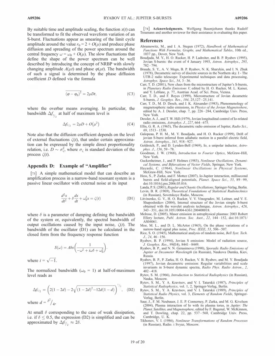
By suitable time and amplitude scaling, the function x(t) canbe transformed to fit the observed waveform variation of anS-burst. Fluctuations appear as smearing of the limit cycleamplitude around the value r0 = 2 + O(m) and produce phasediffusion and spreading of the power spectrum around thecentral frequency w = w0 + O(m). The slow fluctuations thatdefine the shape of the power spectrum can be welldescribed by introducing the concept of NRBP with slowlychanging amplitude A(mt) and phase 8(mt). The bandwidthof such a signal is determined by the phase diffusioncoefficient D defined via the formula

8� 80ð Þ2 ¼ 2mDt; ðC3Þ

where the overbar means averaging. In particular, thebandwidth Df

1=2at half of maximum level is

Df1=2 ¼ 2mDþ O m2� �

ðC4Þ

Note also that the diffusion coefficient depends on the levelof external fluctuations z(t), that under certain approxima-tion can be expressed by the simple direct proportionalityrelation, i.e. D � sz

2, where sz is standard deviation of theprocess z(t).

Appendix D: Example of ‘‘Amplifier’’

[73] A simple mathematical model that can describe anamplification process in a narrow-band resonant system is apassive linear oscillator with external noise at its input

d2x

dt2þ d

dx

dtþ w2

0x ¼ z tð Þ ðD1Þ

where d is a parameter of damping defining the bandwidthof the system or, equivalently, the spectral bandwidth ofoutput oscillations caused by the input noise, z(t). Thebandwidth of the oscillator (D1) can be calculated in theclosed form from the frequency response function

S wð Þ ¼ Abs1

�w2 þ iwd þ w20

:

where i =ffiffiffiffiffiffiffi�1

p.

The normalized bandwidth (w0 = 1) at half-of-maximumlevel reads as

Df1=2 ¼ 2 1� 2dð Þ � 2

ffiffiffiffiffiffiffiffiffiffiffiffiffiffiffiffiffiffiffiffiffiffiffiffiffiffiffiffiffiffiffiffiffiffiffiffiffiffiffiffiffiffiffiffiffi1� 2dð Þ2�12d 1� dð Þ

q 1=2

; ðD2Þ

where d = d2=4,

At small d corresponding to the case of weak dissipation,i.e. if d � 0.5, the expression (D2) is simplified and can beapproximated by Df1=2

2d.

[74] Acknowledgments. Wolfgang Baumjohann thanks RudolfTreumann and another reviewer for their assistance in evaluating this paper.

ReferencesAbramowitz, M., and I. A. Stegun (1972), Handbook of MathematicalFunctions With Formulas, Graphs, and Mathematical Tables, 10th ed.,1037 pp., Dover, New York.

Boudjada, M. Y., H. O. Rucker, H. P. Ladreiter, and B. P. Ryabov (1995),Jovian S-bursts: the event of 4 January 1993, Astron. Astrophys., 295,782–794.

Braude, S. Y., A. V. Megn, B. P. Ryabov, N. K. Sharykin, and I. N. Zhuk(1978), Decametric survey of discrete sources in the Northern sky. I - TheUTR-2 radio telescope: Experimental techniques and data processing,Astrophys. Space Sci., 54, 3–36.

Carr, T. D. (2001), New clues from the microstructure of Jupiter’s S-bursts,in Planetary Radio Emissions V, edited by H. O. Rucker, M. L. Kaiser,and Y. Leblanc, p. 77, Austrian Acad. of Sci. Press, Vienna.

Carr, T. D., and F. Reyes (1999), Microstructure of Jovian decametricS-bursts, J. Geophys. Res., 104, 25,127–25,141.

Carr, T. D., M. D. Desch, and J. K. Alexander (1983), Phenomenology ofmagnetospheric radio emissions, in Physics of the Jovian Magnetoshere,edited by A. J. Dessler, chap. 7, pp. 226–284, Cambridge Univ. Press,New York.

Dessler, A. J., and T. W. Hill (1979), Jovian longitudinal control of Io-relatedradio emissions, Astrophys. J., 227, 664–675.

Ellis, G. R. A. (1965), The decametric radio emission of Jupiter, Radio Sci.,69, 1513–1530.

Galopeau, P. H. M., M. Y. Boudjada, and H. O. Rucker (1999), Drift ofjovian S-burst inferred from adiabatic motion in a parallel electric field,Astron. Astrophys., 341, 918–927.

Goldreich, P., and D. Lynden-Bell (1969), Io, a unipolar inductor, Astro-phys. J., 156, 59–78.

Goodman, J. W. (1968), Introduction to Fourier Optics, McGraw-Hill,New York.

Guckenheimer, J., and P. Holmes (1983), Nonlinear Oscillations, Dynami-cal Systems, and Bifurcations of Vector Fields, Springer, New York.

Hayashi, C. (1964), Nonlinear Oscillations in Physical Systems,McGraw-Hill, New York.

Hess, S., P. Zarka, and F. Mottez (2007), Io-Jupiter interaction, millisecondbursts and field-aligned potentials, Planet. Space Sci., 55, 89 – 99,doi:10.1016/j.pss.2006.05.016.

Landa, P. S. (2001),Regular and ChaoticOscillations, Springer-Verlag, Berlin.Levin, B. R. (1969), Theoretical Foundations of Statistical Radiotechnics(in Russian), Sovetskoye Radio, Moscow.

Litvinenko, G. V., H. O. Rucker, V. V. Vinogradov, M. Leitner, and V. E.Shaposhnikov (2004), Internal structure of the Jovian simple S-burstobtained with the wavelet analysis technique, Astron. Astrophys., 426,343–351, doi:10.1051/0004-6361:200400018.

Melrose, D. (2005), Maser emission in astrophysical plasmas: 2003 RobertEllery lecture, Publ. Astron. Soc. Aust., 22, 144–152, doi:10.1071/AS04061.

Moe, M. L., and D. L. McArtor (1965), On the phase variations of anarrow-band signal plus noise, Proc. IEEE, 53, 506–507.

Rice, S. O. (1945), Mathematical analysis of random noise, Bell Syst. Tech.J., 24, 46–156.

Ryabov, B. P. (1994), Jovian S emission: Model of radiation source,J. Geophys. Res., 99(E4), 8441–8449.

Ryabov, B. P., and N. N. Gerasimova (1990), Sporadic Radio Emissions ofJupiter at Decameter Wavelength (in Russian), Naukova Dumka, Kiev,Russia.

Ryabov, B. P., P. Zarka, H. O. Rucker, V. B. Ryabov, and M. Y. Boudjada(1997), Jovian decametric emission: Regular variabilities and scaleinvariants in S-burst dynamic spectra, Radio Phys. Radio Astron., 2,402–418.

Rytov, S. M. (1966), Introduction to Statistical Radiophysics (in Russian),Nauka, Moscow.

Rytov, S. M., Y. A. Kravtsov, and V. I. Tatarskii (1987), Principles ofStatistical Radiophysics, vol. 1, 2, Springer-Verlag, Berlin.

Rytov, S. M., Y. A. Kravtsov, and V. I. Tatarskii (1989), Principles ofStatistical Radio Physics, vol. 3, Elements of Random Fields, Springer-Verlag, Berlin.

Saur, J., F. M. Neubauer, J. E. P. Connerney, P. Zarka, and M. G. Kivelson(2004), Plasma interaction of Io with its plasma torus, in Jupiter: ThePlanet, Satellites, andMagnetosphere, edited by F. Bagenal, W. McKinnon,and T. Dowling, chap. 22, pp. 537–560, Cambridge Univ. Press,Cambridge, U. K.

Tikhonov, V. I. (1986), Nonlinear Transformations of Random Processes(in Russian), Radio. i Svyaz, Moscow.


19 of 20

A09206

Willes, A. J. (2002), Jovian S burst drift rates and S burst/L burst interac-tions in a phase-bunching model, J. Geophys. Res., 107(A5), 1061,doi:10.1029/2001JA000282.

Wu, C. S., and L. C. Lee (1979), A theory of the terrestrial kilometricradiation, Astrophys. J., 230, 621–626, doi:10.1086/157120.

Zarka, P. (1998), Auroral radio emissions at the outer planets: Observationsand theories, J. Geophys. Res., 103, 20,159–20,194.

Zarka, P., T. Farges, B. P. Ryabov, M. Abada-Simon, and L. Denis (1996),A scenario for Jovian S-bursts, Geophys. Res. Lett., 23, 125–128.

Zarka, P., J. Queinnec, and F. Crary (2001), Low-frequency limit of Jovianradio emissions and implications on source locations and Io plasma wake,Planet. Space Sci., 49, 1137–1149.

��R. Kozhin, B. P. Ryabov, V. A. Shevchenko, D. M. Vavriv, and V. V.

Vinogradov, Institute of Radio Astronomy, 4 Krasnoznamennaya St.,610002 Kharkov, Ukraine.V. B. Ryabov, Future University-Hakodate, 116-2 Kamedanakano-cho,

Hakodate, Japan 041-8655. ([email protected])P. Zarka, Laboratoire d’Etudes Spatiales et d’Instrumentation en

Astrophysique LESIA, Paris Observatory, F-92195 Meudon, France.


20 of 20

A09206

jupiter s-bursts: narrow-band origin of microsecond subpulses

Documents