journal of hydrology: regional studies - research @ flinders

Contents lists available at ScienceDirect

Journal of Hydrology: Regional Studies

journal homepage: www.elsevier.com/locate/ejrh

A socio-environmental model for exploring sustainable watermanagement futures: Participatory and collaborative modelling inthe Lower Campaspe catchmentTakuya Iwanagaa,*, Daniel Partingtonb, Jenifer Ticehursta, Barry F.W. Crokea,c,Anthony J. Jakemanaa Fenner School of Environment and Society, Institute for Water Futures, The Australian National University, Canberra, AustraliabNational Centre for Groundwater Research and Training, Flinders University, Adelaide, AustraliacMathematical Sciences Institute, The Australian National University, Canberra, Australia

A R T I C L E I N F O

Keywords:Integrated modellingParticipatory modellingExploratory modellingScenario discoveryConjunctive water use

A B S T R A C T

Study region: Lower Campaspe, North Central Victoria, AustraliaStudy focus: This paper presents a component-based integrated environmental model developedthrough participatory processes to explore sustainable water management options. Possible fu-tures with improved farm profitability and ecological outcomes relative to modelled baselineswere identified through exploratory modelling. The integrated model and the results producedare intended to raise awareness and facilitate discussion with and amongst stakeholders.New hydrological insights: The modelling illustrates that improved farm level knowledge andmanagement with regard to crop water requirements, soil water capacity, and irrigations are themost significant factors towards achieving outcomes that are robust to a range of climate andwater policy futures. Assuming farmer management with regard to these factors are at their mostoptimal, increasing irrigation efficiency alone did not lead to improved farm profitability andecological outcomes under drier climate conditions. Likelihood of achieving robust outcomeswere further improved through the conjunctive use of surface and groundwater, with increasedconsideration of groundwater use a key factor. Further discussion on the viability and impact ofincreased groundwater use and conjunctive use policies should be further considered.

1. Introduction: Sustainable water management and aims of the integrated modelling

Management of water resources takes place within the context of a complex socio-environmental system. Sustainable manage-ment of water resources requires the needs of several agricultural, environmental, and social domains to be balanced with explicitconsideration of a multitude of interacting factors. Here, “sustainable” refers to water usage that is both beneficial and robust -featuring improved farm profitability and environmental outcomes and maintaining these under changing, possibly adverse, climaticconditions within hypothetical policy contexts (revisited in Section 4).

Holistic modelling of this socio-environmental system then requires an integrated approach due to the number of system domainsunder consideration, the level of interactions that can occur at different (spatial and temporal) scales, and the uncertainty that comeswith it (Letcher et al., 2007; Schlüter et al., 2019). A well-considered integrated approach can reduce the risk of unintentionally

https://doi.org/10.1016/j.ejrh.2020.100669Received 4 December 2019; Received in revised form 29 January 2020; Accepted 1 February 2020

⁎ Corresponding author.E-mail address: [email protected] (T. Iwanaga).

Journal of Hydrology: Regional Studies 28 (2020) 100669

Available online 21 February 20202214-5818/ © 2020 The Authors. Published by Elsevier B.V. This is an open access article under the CC BY license (http://creativecommons.org/licenses/BY/4.0/).

T

http://www.sciencedirect.com/science/journal/22145818

https://www.elsevier.com/locate/ejrh

https://doi.org/10.1016/j.ejrh.2020.100669


mailto:[email protected]


http://crossmark.crossref.org/dialog/?doi=10.1016/j.ejrh.2020.100669&domain=pdf

disregarding crucial aspects of the management context and the flow-on effects without which the conclusions reached may becompromised (Kelly et al., 2013). To this end Integrated Environmental Models (IEMs) are often constructed to aid in informingmanagement and policy decisions (Elsawah et al., 2020a; Janssen et al., 2010; Voinov and Shugart, 2013).

Stakeholder engagement is an important step in integrated modelling, particularly in developing socio-economic scenarios thatare acceptable and relevant to stakeholders. Such participatory approaches within water resource modelling processes are nowconsidered best practice in facilitating stakeholder buy-in, credibility of the modelling and integration of local knowledge andinformation into the model (Kelly et al., 2013; Megdal et al., 2017; Refsgaard et al., 2007). To holistically develop the model, anapproach such as the one described in Badham et al. (2019) can be used to elicit stakeholder knowledge to aid in defining theproblem frame and key issues.

The Murray-Darling Basin Plan (introduced in 2012) increases the amount of water allocated for environmental purposes bydecreasing the volume for consumptive use (Bowler, 2015; North Central CMA, 2014). The intention of the Plan is to rectify theobserved long-term degradation of environmental health of river systems within the Murray-Darling Basin generally. To this end,beneficial future scenarios would improve, or at least maintain, current levels of water availability for agricultural, environmental,and recreational purposes in the face of uncertain future climate conditions.

The primary aims of the study presented within this paper were to identify these future pathways (“scenarios”) to improvedenvironmental and socio-economic outcomes under a variety of climate conditions for the Lower Campaspe catchment in NorthCentral Victoria (Australia). On-farm practices and water allocation policies were modelled and an exploratory modelling approach(Haasnoot et al., 2013) adopted to identify these possible robust outcomes. Such scenario discovery approaches have been utilisedpreviously to identify viable adaptation strategies with indication of trade-offs between scenarios (Kwakkel et al., 2016).

The variety of data and knowledge sources, number of systems involved and the interactions and feedbacks between themrequired to represent such a system made the use of an integrated model a natural fit. An IEM was developed for the study, which werefer to as the CIM (Campaspe Integrated Model). The CIM includes representations of relevant systems across the socio-environ-mental spectrum and their interactions. These include policy, farm, surface and groundwater hydrology, ecology, and recreationalvalues. Climate factors are represented by rainfall and evapotranspiration data, which drive the modelled system. The CIM is used toexplore the mix of considered farm and policy level options that are robust in the long-term, in terms of successfully achievingdesirable improvements from a baseline across climate scenarios. In this paper we detail the model components developed, discussthe integration process, and finally present the model results and their implications. The specifics of the management context andmodelling process are reported in Iwanaga et al. (2018), however relevant elements will be repeated herein for context.

2. Lower Campaspe study area

The Lower Campaspe study area is a semi-arid region situated in the North-Central region of Victoria, Australia and is named forits primary river (the Campaspe), which flows northwards, joining the Murray River. The primary water source for the LowerCampaspe is the dam at Lake Eppalock, which divides the Campaspe into its Lower and Upper sub-catchments. The dam is operatedby Goulburn-Murray Water (GM Water) subject to local and federally mandated policies such as the aforementioned Murray-DarlingBasin Plan. Under current policies the environment is regarded as a water user with its own water entitlements (North Central CMA,2014). Aside from managing dam operations and other responsibilities GM Water is the local irrigation authority, determining waterallocations (for both agricultural and environmental users) and managing licencing for water use and access.

The Campaspe catchment is a mixed-farming area with a focus on dairy farming, with 55 % of its land use devoted to annual andperennial pastures. Cereal cropping amounts to 36 % of reported agricultural land area. Fig. 1 displays a map of the Lower Campaspein context of the North Central region and the Murray-Darling Basin. Historically the Campaspe region was an irrigation intensivearea, but a decade-long drought – the Millennium Drought – reduced water availability such that 90 % of irrigators elected to ceaseirrigation practices in 2010 (North Central CMA, 2014; NVIRP, 2010). Approximately 38 % of the Lower Campaspe is under drylandfarming (Ticehurst and Curtis, 2016) with the north of the catchment focused on cropping activities (depicted in Fig. 1).

Water resources have been described as historically over-allocated for agricultural purposes, and the possibility of a drier climatein the future (van Dijk et al., 2013v) implies balancing available water resources between competing needs and interests is expectedto become increasingly difficult. Ecological health of the Campaspe river system has been in decline over the past decades as waterwas historically prioritised for agricultural purposes. This has had the effect of substantially decreasing local biodiversity (MDBA,2012; North Central CMA, 2014). Communities of the iconic River Red Gum eucalypts, platypus colonies, and populations of nativefish (such as the Murray Cod and Golden Perch) exist along the Lower Campaspe system.

Recent water reforms have included provisions for increased environmental flows to support recovery and maintenance ofecosystem health (GHD, 2015; GM-W, 2013; Hughes et al., 2015). Water to support environmental flows include 75 G L reallocatedfrom agriculture as well as estimated water savings due to infrastructure improvements conducted through the Goulburn MurrayConnections project (NVIRP, 2011). Recreational use of the dam is an additional area of concern, with viability of recreationalactivities (e.g. boating and yachting) suffering as the water levels at Lake Eppalock fall. There has been public outcry in this regard, asevidenced by local media reports (ABC News, 2015; Wines, 2015).

Decisions made in managing the lower Campaspe River affect river systems downstream, the Campaspe being a tributary of theMurray. Therefore, beneficial ecological outcomes within the Campaspe are likely to support ecological recovery elsewhere down-stream. The CIM was designed and developed to inform management and decision-making processes within this context through anexploratory process.

T. Iwanaga, et al. Journal of Hydrology: Regional Studies 28 (2020) 100669

2

3. Integrated model development

To explore possible futures in the Campaspe, changes to on-farm practices and water allocation policies were modelled and thesubsequent effects on farmer income, streamflow conditions for platypus colonies, native fish and river red gums (trees), and re-creational use of the dam were analysed. Specifically, these scenarios represent the conjunctive management of both surface andgroundwater (Pulido-Velazquez et al., 2011), encouragement of further use of groundwater resources in general, and further im-provements to irrigation (water application) efficiency (Ticehurst and Curtis, 2017, 2016). The CIM comprises models to representclimate sequences, policy rules, agricultural activities, surface and groundwater hydrology, and indicators of ecological and re-creational suitability. Individual model domains deal with their own unique issues and conceptualise the system, and their inter-actions with other models, in separate ways. This is most obvious in the represented spatial and temporal scales. In building the CIM,compromises were necessary in order to suit the purpose of the modelling and in the face of inter-linked requirements and availableresources. For this reason, further detailed framing of each model domain and, where relevant, model inputs and indicators of interestare described in the sub-sections below.

3.1. Stakeholders and engagement process

As noted in the introduction, engagement with local stakeholders was particularly important to both the development and va-lidation of the CIM. Relevant stakeholders were identified through sectoral interests and relevance (e.g. farmers will be interested inpolicies that affect farming), as well as a snowball sampling approach where known experts where recruited to suggest other expertsof interest relevant to the study. Stakeholders involved both prior to and during the modelling process included local farmers, GMWater, and representatives from government departments and non-profit organisations. These represent actors within the system that

Fig. 1. Map of the Lower Campaspe catchment (left panel) in relation to the Murray-Darling Basin (top right) and the North Central Region ofVictoria (bottom right). The Lower Campaspe constitutes the area north of Lake Eppalock, which is the primary reservoir for the study area. TheCampaspe River flows south to north, into the Murray River.


3

use the water, managers of the water, and those with specialised knowledge of the system, including farm management and irrigationspecialists, ecologists, geo-hydrologists and catchment managers to name a few.

A stakeholder group of representatives from GM Water, the local Catchment Management Authority (North Central CMA) and arelevant state government department (at the time, the Department of Economic Development, Jobs, Transport and Resources)attended workshops to identify potential opportunities for conjunctive use in the region. Farmers were engaged through interviewsand surveys prior to model development, details of which can be found in Ticehurst and Curtis (2017, 2016). This engagementidentified the current and future intention to adopt various management options including the use of groundwater, various irrigationpractices, and the technical feasibility and social acceptability of the range of conjunctive use opportunities identified in previousworkshops. GM Water also provided irrigator data and aided in defining the spatial scope and boundaries of the study with respect tothe represented groundwater catchment and management zones. The stakeholder group also took part in later workshops and servedto provide information and knowledge which corrected earlier assumptions and provided further feasibility assessment of on-farmscenarios. Issues and concerns surrounding ecological aspects were elicited through engagement with ecologists from the AustralianPlatypus Conservancy and the North Central CMA. Further details may be found in Iwanaga et al. (2018).

3.2. Technical implementation

A requirement of the integrated model development was to be flexible in the face of changing and evolving understanding of thesystem due to the amount and spread of knowledge being engaged with through the participatory engagement process that wasdescribed in the previous section. To facilitate this an iterative component-based approach was adopted in the development of theCIM. Construction of the CIM involved the use of a mix of programming languages including Fortran and Python (and its compiledcousin Cython), incorporation of pre-existing models, and the development of a purpose-built (software) framework through whicheach component model was coupled.

Interfaces (commonly referred to as wrappers) were developed for the purpose of invoking component model runs and thusprovide the necessary linkage between the framework and the component models. Fig. 2 depicts the inter-relationship between thecomponent models. Inter-model communication (i.e. data exchange) occurs with the framework acting as an intermediary. Con-version of data, such as between types or units of measurement, occurs where necessary and is specifically coded. While not adheringto all aspects, the structure of the interfaces is similar to those specified by the Basic Modeling Interface (Peckham et al., 2013) in thateach interface provides a method to invoke a run of the component model for a given time step. This design pattern was selected forits flexibility, simplicity and ease of implementation. Component models are run as a serial process with one model run after theother, with feedback occurring across (daily) time steps. Further details on the choice of modelled spatial and temporal scale is givenin later sub-sections for each system component.

Fig. 2. Component diagram indicating the interactions between model components in the Campaspe Integrated Model (CIM) and the key outputsrelevant to the modelled Lower Campaspe system.


4

Currently, the model takes approximately 30 min. to run for a single scenario on a desktop computer with a Core i5-7500 CPU.The groundwater model based on MODFLOW-NWT is run as an external program and is currently the primary bottleneck limitingfurther increases to runtime efficiency. Although MODFLOW itself is written in Fortran – considered to be a “fast” language –numerical solution of groundwater models is time consuming and the MODFLOW software itself uses several input files which mustbe written out for each time step and the results read back in. Overheads due to the constant file operations takes a large proportion ofthe runtime. As much as 43 % of the CIM runtime can be attributed to the groundwater model. MODFLOW’s position as an industrystandard was the primary reason for its use.

The exploratory approach conducted for the study involved many runs and so the CIM was designed to run multiple scenarios inparallel in order to overcome computational runtime issues. Model runs are invoked via the command-line and is compatible withboth Linux and Windows systems. No graphical user interface was developed for the study as use by non-technical “end-users” wasnot planned and is not expected.

3.3. Climate and scenarios

Changes in rainfall and temperature influence water availability and their trends can impact the volume of irrigation waternecessary to achieve optimum crop growth and yield throughout a growing season. The importance of considering climatic influencesin managing farm processes is reflected in the survey conducted by Ticehurst and Curtis (2016). Over 80 % of respondents rankedchange in rainfall patterns and the impact of drought as “important” or “very important”.

Comparing long term (100 year) average growing season rainfall against more recent trends highlights the impact of theMillennium Drought (1996–2010). A growing season refers to the time span in which crops are usually sown and harvested, definedhere as May to February. Average long-term growing season rainfall between 1892–2013 amounted to ∼420 mm in line with thereported usual growing season rainfall of 400–500 mm (EcoDev, 2015). Growing season rainfall from 1982 to 2016 however shows adecrease of 67 mm to ∼353 mm (see Fig. 3). The trend of decreased rainfall during crop growth may continue with agricultural watermanagement becoming increasingly challenging.

To investigate the impacts of a changing climate, historic and future climate data were sourced from the Climate Change inAustralia data service (https://www.climatechangeinaustralia.gov.au; CSIRO, 2017). The provided datasets consist of daily rainfalland evapotranspiration in 5 km grid format for a 30-year period. The future climate data provided were developed through a processof scaling historic observations (described in Mitchell, 2003) and thus exhibit similar rainfall trends to historic observations. Pearsoncorrelations between climate scenarios are depicted in Fig. 4 with a minimum correlation value of 0.88 and 0.99 for rainfall andevaporation data respectively. Future climate datasets are based on the historic timeframe from 1981 to 2011, and thus cover theMillennium Drought period. Therefore, each climate scenario includes a representation of a multi-year drought at differing levels ofseverity. For the purpose of calibration and analysis, the historic climate dataset was extended to 2016 in order to capture the post-drought recovery. The set of climate scenarios covers RCP4.5 and 8.5 for 2016–2045, 2036–2065 obtained from multiple climatemodels, “best case”, “worst case” are wettest and driest across models, whilst “maximum consensus” represents conditions somewhatcomparable to historic experience.

To determine the range of conditions that the climate sequences represent, the aridity index (AI ) developed by the UN

Fig. 3. Comparisons of growing season rainfall over the long-term (100+ years, left panel) and a shorter (30+ year) period (right panel). Dashedblack line indicates median values which were found to be 420 mm over the long term which reduced to 353 mm in the recent past (1982–2015growing seasons) indicating the effect of the Millennium Drought. Long term data were developed through interpolated historic rainfall data (seeVaze et al., 2011).


5

https://www.climatechangeinaustralia.gov.au

Environment Programme (UNEP) was used to compare the climate scenarios. The index is calculated as P PET/ , where P is the annualaverage rainfall and PET is the annual average potential evapotranspiration (Gamo et al., 2013). An AI value of 0.2 to 0.5 indicates asemi-arid climate condition (Sahin, 2012), and the AI value for the historic climate dataset falls within these bounds with a value of0.34, as is expected for this semi-arid location.

Of the procured climate datasets, the driest conditions are represented by the notation “worst_case_rcp45_2016-2045″ ( =AI 0.26).The “best_case_rcp45_2016-2045″ scenario was most comparable to historic aridity ( =AI 0.34), while “best_case_rcp45_2036–2065”was the least arid ( =AI 0.35). The indicated climate scenarios are taken to represent the extremes of future climate variability (i.e.the most and least arid conditions) and one that is most similar to historically observed conditions. For this reason, modelling withthe other climate scenarios were not conducted in-depth. Interpolation between the extremes would likely provide indicative in-termediary results. These climate scenarios are referred to as “wet”, “usual”, and “dry” for brevity from here on and were used todrive the CIM in order to investigate the impact of such changing climate conditions.

3.4. Policy model

Significant reforms to the water policy in the Campaspe introduced water trading, user carryover (specified below), and en-vironmental water provisions (Alston and Whittenbury, 2011; McKay, 2005; Wheeler and Cheeseman, 2013). As part of these reformsthe environment is regarded as a water user with water entitlements and yearly water allocations similar to any other entity with awater licence. The policy model provides representations of policies that determine water allocation and carryover.

Access and use of water resources are governed by a licencing system in which a licence held by a water user specifies a givenvolume of water called an entitlement. Separate licences are issued for surface and groundwater. Access to the full entitlement is notguaranteed and is subject to water availability. An allocation is announced by GM Water each irrigation season indicating thepercentage of the entitlement an irrigator can use – i.e. 100 % allocation is equal to the full entitlement volume. Carryover here refersto the amount of unused water allocation which licence holders (irrigators and the environment) are able to add to the followingyear’s allocation.

Current carryover rules indicate that irrigators are able to carry over 95 % of unused surface water, with 5 % deducted to accountfor evaporation loss (DSE, 2012a, 2012b), and 25 % of unused groundwater (Goulburn-Murray Water, 2015). While irrigators candecide not to carryover (DSE, 2012b), it is assumed in the model that carryover always occurs. As indicated in Fig. 2, the policy modeldictates availability of water for agricultural and environmental purposes and is itself influenced by climate conditions, dam andgroundwater levels.

3.4.1. Surface water policySurface water allocations in the Lower Campaspe are calculated based on the available volume of water in the dam as well as

projected inflows. GM Water holds rights to 82 % of the dam volume as well as 82 % of projected inflows and the sum of these is used

Fig. 4. Pearson correlation matrix between future climate scenarios and historic observations.


6

to calculate the total allocation for the Lower Campaspe catchment. The allocation is announced on 1 July and is re-calculatedthroughout the irrigation season. As such, a water user’s allocation may increase over the course of the growing season if larger-than-expected rainfall and inflows occur, and so the volume of allocations will not decrease retrospectively. Dam operation requirementsas dictated by local policy and legislative rules, including environmental watering and minimum flow rules, are also factored into theallocation calculations. The model represents this process on a two-week basis (rather than 6-weekly as happens in reality) to allowfor better interoperation with the farm model.

A complication in the surface water policy model is the fact that irrigators in the Lower Campaspe hold additional licences forwater from the neighbouring Goulburn catchment (east of the Campaspe). Rather than model another catchment in its entirety, linearrelationships at three different levels were developed between the Campaspe and Goulburn allocations. Details on this relationshipmay be found in Appendix C. These are referred to as “high”, “median” or “low” and represent the level of allocation volumeavailable from the Goulburn catchment for a modelled future scenario. The separate allocation scenarios allow the model to accountfor conditions which influence availability of water from the Goulburn including variability between the two catchments. Thesedifferent conditions may be due to climate variability, water demand, and policies that affect Goulburn allocations which in turn mayaffect the indicators of interest for the Lower Campaspe. Associated costs were assumed to be identical to that of GM Water. Waterentitlements for individual farm zones (detailed in Section 3.5 below) are shown in Table 1 and were calculated by proportionallydistributing the entitlement based on the Water System area under which the given zone falls under.

3.4.2. Groundwater policyGroundwater allocations are restricted by policy rules surrounding what are referred to as “trigger levels”. These indicate the

groundwater level at which allocations are reduced to a specified percentage or, at its lowest level, no allocation at all. Groundwateruse is progressively restricted in this manner as the water table decreases in order to prevent salinity intrusion. Allocations aredetermined based on the recorded groundwater level at two reference bores with the IDs 62589 in the south and 79324 in the northGoulburn-Murray Water, 2015) and are detailed in Table 2 (under “Current Modelled Allocation”).

Table 1Campaspe entitlements in ML for each farm zone used in the modelling (see Fig. 6). Entitlements for a given water system were proportionallydistributed based on zonal area.

Zone ID High Reliability Entitlement(ML)

Low Reliability Entitlement(ML)

Goulburn High Reliability Entitlement(ML)

Water System Name

1 0 0 0 –2 12050.87 4008.06 0 Campaspe River (Eppalock to

Weir)3 0 0 0 –4 5703.12 1896.83 0 Campaspe River (Eppalock to

Weir)5 0 0 0 –6 1086.30 353.10 0 Campaspe River (Weir to WWC)7 674.90 383.80 215.10 Campaspe Irrigation Area8 46.71 7.68 39249.62 Rochester Irrigation Area9 707.05 0 0 Campaspe River (WWC to Murray)10 96.68 15.91 81223.37 Rochester Irrigation Area11 224.44 0 0 Campaspe River (WWC to Murray)12 0 0 0 –

Table 2Groundwater allocation rule sets (current and hypothetical). Reduced allowable allocations under surface water allocations> 60 % or 80 % de-pending on scenario then saves water for use in dry (drought) periods. Groundwater head at reference bores influence allocations for separate Zones.

Proposed Trigger Rules

Farm Zone(s) Reference bore Depth from naturalsurface (m)

Water level(mAHD)

Current ModelledAllocation

Non-droughtAllocation*

Drought Allocation

3 – 12 79324 0 – 16 82.1 – 97.1 100 % 80 % or 100 % 100 %16 – 19 79.1 – 82.1 75 % 65 % 100 %19 – 22 76.1 – 79.1 50 % 35 % 100 %22 – 25 73.1 – 76.1 40 % 25 % 40 %< 22 < 73.1 0 % 0 % 0 %

1 and 2 62589 0 – 16 115.8 – 131.8 100 % 80 % or 100 % 100 %16 – 18 113.8 – 115.8 75 % 65 % 100 %18 – 20 111.8 – 113.8 50 % 35 % 100 %< 18 < 111.8 0 % 0 % 0 %

* non-drought is defined as>60 % or> 80 % surface water allocation as a scenario option.


7

In the current policy context surface and groundwater are managed separately, however stakeholders have explicitly suggested amove towards a conjunctive management approach. A possible change in the policy space includes the relaxation of trigger levelsduring dry periods (thereby enabling irrigators to use more groundwater) followed by compensatory actions to increase rechargeduring wet periods. Hypothetical trigger rules for conjunctive use were developed for the model. These rules define two sets of triggerlevels (referred to as the “drought” and “non-drought” rulesets) and management is switched between these depending on the surfacewater allocation. “Drought” trigger rules come into effect after consecutive years of surface water allocations below 60 % or 80 %.Depending on scenario, this may be after 1 or 3 years after which irrigators are able to use their full groundwater entitlement for allbut the lowest trigger level. These are detailed in Table 2 and referred to collectively as the “proposed trigger rules”.

Farmers surveyed in the area have indicated that such increased use of groundwater is technically feasible. Most irrigators arereliant on surface water resources, with 91 % of those surveyed holding surface water licences compared to 22 % who additionallyhold groundwater licences (Ticehurst and Curtis, 2017). Groundwater use historically has reached a maximum of 60 % of allocatedvolumes, although this has increased to 80 % in recent times (2016 water usage as reported in Ticehurst and Curtis, 2017). Recallingthat 25 % of unused water can be carried over, the current view is that irrigators are reserving water for drier times accepting a trade-off between enhanced yields in wet years in return for water security in dry conditions. Hence the farming community could bedescribed as managing water resources in a conjunctive manner, albeit informally.

The CIM includes a scaling factor (60–100%) to adjust the amount of allocated groundwater considered for use by the farm modelto reflect this informal management approach. Note that setting the scaling factor to 100 % only makes all groundwater available, itdoes not enforce its use. Limiting allocation to 60 % then reflects a return to historic behaviour in which farmers intentionally reservewater to enhance future water security.

Water usage and its impact is indicated with percentage increase or decrease in water use (both ground and surface water)compared to the baseline scenario, and the long-term decline (or improvement as the case may be) in terms of depth to groundwateracross the farm zones. In addition, two quantities of interest relate to groundwater: average groundwater allocation (“GW AllocationIndex”) and the relative depth to groundwater (head), normalised by the lowest trigger level at each reference bore and averaged overthe time series (“GW Level Change”). Average allocations indicate reductions in access to groundwater, whereas the change inrelative depth provides an indication of how sustainable groundwater use is under the given condition. Negative changes to the GWLevel Change imply increased reliance on groundwater and/or reduced groundwater recharge. Notable model inputs are given inTable 3.

3.5. Farm model

The farm model represents the agricultural system by dividing the catchment into 12 Zones based on their water entitlements,policy rules governing water allocations, and land use (depicted in Fig. 6), corresponding to the Management Zones in use by GMWater (see Goulburn-Murray Water, 2015). Key attributes of a modelled farm include the costs and capital returns of crop sown,nature and cost of irrigation and pumping systems, and the soil water holding properties of the soils found within the Zone. Themodel focusses on cropping enterprises; water use for dairying is not considered here. Cropping is modelled as a three year rotation ofwheat, barley and canola. Further details on the model formulation are provided in Appendix B.

Irrigation systems considered in the model include gravity, pipe and riser, and spray. These represent the cheapest and least waterefficient to the most expensive and efficient option available to farmers. Gravity is regarded as the dominant form of irrigation in theLower Campaspe, although it is known through stakeholder feedback that there is increasing adoption of spray irrigation in the area.Parameters representing soil water capacity were raised by stakeholders as particularly important as they determine what irrigationsystem is suitable and influence frequency of irrigation events. Farms with sandier soils see a greater benefit from a switch to moreefficient irrigation systems as such soils have a lower water retention capacity. While farmers cannot change the soil type, it ispossible to improve soil health such that water retention is enhanced through best management practices (Bruyn, 2019). Table 4 liststhe considered irrigation options for each farm zone based on the weighted zonal average soil water capacity. For the presentedstudy, only Zones 4 and 9 were modelled as being suitable for spray irrigation.

Farmer decisions are modelled through linear programming at the start of and during a growing season. The available area isallocated to dryland cropping and irrigation with surface and groundwater by optimising profit calculated with assumed per hectarerevenues and costs, constrained by water availability. The model then optimises for profitable water usage for each subsequent (two-

Table 3Policy model inputs of interest and their description.

Factor Name Description

restriction Groundwater allocation ruleset (“current” or “proposed”) used for the scenario run.drought_trigger Surface water allocation threshold for switching to the proposed allocation ruleset under conjunctive use scenarios (see

restriction factor above), defined as a percentage of entitlements. Either 60% or 80%.max_drought_years The number of years surface water allocations must be below drought_trigger before switching allocation ruleset. Either 1 or 3.goulburn_allocation_scenario Assumed allocation relationship between Campaspe and Goulburn (“high”, “median”, or “low”). Informs allocation volume

from the Goulburn catchment.gw_cap Scaling factor limiting the volume of groundwater allocation the farm model considers. Set to 100 %, but can vary between

60–100%.


8

week) time step for each farm zone until the pre-determined harvest date. Again, further details of the model formulation are given inAppendix B.

The assumption of this approach is that a series of short-term decisions that are financially sound will result in a profitableoutcome. The two-week time step was also necessary to facilitate representation of cross-domain interactions as agricultural irri-gation/pumping activities influence stream and groundwater systems. All events (irrigation, planting/sowing, harvest) are assumedto take place within two week periods.

In terms of interactions with other component models, the farm model is influenced by the water allocation determined by thepolicy model, and subsequently influences the surface and groundwater models through irrigation water extraction (pumping andirrigation activities). Further interaction with the policy model is included due to local policies allowing carryover in which a portionof unused water is made available to irrigators in the following year.

From the perspective of the farm model, three categories of factors can be identified: uncontrollable, limited control, and directcontrol. Uncontrollable factors are those that cannot be influenced in any direct manner such as climate condition, water allocations,or crop water requirements. Limited control factors are those which a farmer may influence to some degree, such as how much watera soil type can hold, by applying soil management practices. Direct control factors are those that a farmer can influence directly, suchas the irrigation system in use, their efficiencies (through irrigation design and monitoring), and so on.

Groundwater cap (`gw_cap`) is a model input of note, and acts to force the model to limit available water for consideration by thefarm model. As noted above in the groundwater policy section (Section 3.4.2), only 60 % of allocated groundwater has been used byirrigators in the past. The considered parameter range was 60–100%, where 60 % represents past behaviour and 100 % reflectsconsideration of all available groundwater for use without regard to future water security. The cap can be applied in combinationwith the conjunctive management scenario detailed in Section 3.4 above.

Three key indicators were used to represent farm performance: 1) the average seasonal farm profit for the scenario, 2) the averageseasonal water use in ML, and 3) the coefficient of variation ( µ/ ) for farm income taken as a measure of fluctuations in yearly income(i.e. a volatility index). Larger values for the volatility index indicate scenarios in which farm income undergoes large variations fromyear to year. Irrigation area (relative to catchment area) and water use are also included.

3.6. Surface water model

The surface water system is represented by a purpose-built variant of the IHACRES rainfall-runoff model (Croke and Jakeman,2004) written in Fortran and interfaced with a Python wrapper. The component model comprises a rainfall-streamflow model, arouting module and a rating curve module. The component is driven by rainfall and potential evapotranspiration (climate data),estimated groundwater and surface water interactions (from the groundwater component), dam releases (as given by the policy andfarm components) and water extractions from the stream (farm component). As water orders are lumped due to the farm modeloperating on a two-week time step, the volume extracted is disaggregated uniformly across the 14 days as a daily average.

Effective rainfall i.e. rainfall that contributes to streamflow is calculated from rainfall via a non-linear loss module from Croke andJakeman (2004), modified to partition effective rainfall between quick and slow flows based on modelled catchment moisture status(Croke et al., 2015). Movement of water through the river network is represented by two parallel exponentially decaying storesrepresenting quick and slow flow contributions. A further exponentially decaying store is used to route the flows between nodes(Croke et al. 2006). Modelled flows are converted to stage heights by the rating curve module using data available at most gauge sites.The single exception is gauge 406218 where available data were limited to water level. Losses from the river network to groundwaterare considered via interactions with the groundwater component, similar to the approach in Ivkovic et al. (2014).

Dam level, streamflow and level were important quantities to represent as these influence water allocations, ecological health,

Table 4Irrigation options considered for each farm zone. All zones can also consider switching to dryland farming. Zones 1, 3, 5 and 12 are modelledwith no water entitlements and are assumed to be dryland only. Assumed efficiency ratings for each are given in brackets (see details inAppendix B). See Zone definitions in Fig. 6.

Irrigation Option

Zone Gravity (50–90 %) Pipe and Riser (70–90 %) Spray (80–90 %)

1 –2 ✓ ✓3 –4 ✓ ✓ ✓5 –6 ✓ ✓7 ✓ ✓8 ✓ ✓9 ✓ ✓ ✓10 ✓ ✓11 ✓ ✓12 –


9

and recreational use of the dam (described in later sections). Stream flow and level are estimated at specific nodes (show in Fig. 7)which were selected based on the location of gauges with suitable data, taking into consideration the needs of the integrated model(see Fig. 2). These values are passed to the groundwater model in order to estimate infiltration loss and baseflow contribution tosurface flow.

Calibrating the model against historic observations proved difficult due to variation of parameter values estimated depending onclimate sequence, and so a decision was made to divide the climate sequence into six time periods and calibrate parameter values foreach separately using the Differential Evolution algorithm (Storn and Price, 1997). A good fit with historic dam levels was achievedwith this approach (with a NSE value of 0.96, depicted in Fig. 8). Calibrated values were then used for the corresponding time periodsfor all climate scenarios. Each set of parameters have a limited scope of applicability, but their use for the segmented time periods isarguably justified for the modelling purpose as similar patterns can be associated with the provided climate scenarios (as previouslydescribed in Section 3.3). Time periods defined for calibration purposes are detailed in Appendix D.

3.7. Groundwater model

The groundwater component serves two roles in the CIM. The first is to provide estimations of the exchanges between surfacewater and groundwater along the Lower Campaspe River at specific gauge locations. The second is to provide estimations of thegroundwater levels for each farm zone and at specific bore locations, which influence allocations of groundwater and pumping costsand is a factor in the ecological indicator metric (see Section 3.8). Interactions at a daily time step with the surface water, farm,ecology, and policy components are included in this manner, and are forced by rainfall, irrigation, pumping, and river stages (de-picted in Fig. 9).

Stakeholders provided knowledge and data with respect to pumping, observational groundwater head, and chemistry, whichinformed the groundwater model boundaries ensuring that the necessary spatial area is captured in the model. The groundwatermodel represents the Lower Campaspe at a 5 km grid resolution with 7 layers comprising 1386 active cells, spacing of which wasinformed by hydrogeologic unit rasters from the Victorian Aquifer Framework DSE, 2012c). The relatively large grid resolution wasselected as 1) it aligns with the provided climate data, and 2) for computational reasons, as higher resolutions required prohibitivelylonger run times.

MODFLOW-NWT (Niswonger et al., 2011) was used to construct the groundwater component and is interfaced with via the Flopypackage (Bakker et al., 2016). MODFLOW was selected due to its open-source and well-documented nature, which complements ouriterative development, and because the modelling platform is regarded as an industry standard. Modelled groundwater extraction isdistributed across known wells within each farm zone. Response to input from the streamflow lags the surface water model ascomponent models are run sequentially. It is assumed that the daily lag will not have a significant impact on model behaviour.Recharge is derived by multiplying the sum of rainfall and irrigation by a rainfall reduction parameter between 0 (no recharge) and 1(no diversion) with values being in the range of 0.001 – 0.43. These rainfall reduction values were derived from a map of rechargeranges for recharge zones defined by rainfall, land use and soil type (detailed in Xie et al., 2019).

Outputs from the groundwater model, while not precise at the scale of local wells due to model resolution, were fit for purpose forindicative average groundwater levels in areas of interest. In the case of the ecology model, the requisite groundwater heads obtainedfrom the groundwater model would be subject to the largest variance due to the proximity to the Campaspe River and variability ofheads within a groundwater model cell. For the policy model the trigger bores are chosen to be indicative of larger scale behaviour,and hence the use of the average head in cells that correspond with the trigger bores is deemed appropriate.

Effectiveness of policies in maintaining groundwater levels above the lowest trigger level is indicated by two metrics. The firstindicator is a weighted score based on the percent irrigation season allocation across the scenario period (GW Allocation Index)where a score of 1.0 indicates that water users were given 100 % of their entitlements every year, and values close to zero indicateconsistently low water table such that pumping is disallowed. The second indicator (GW Level Change) is the averaged normalisedchange in groundwater level between the start and the end of the model period relative to the lowest trigger level. Negative valuesthen indicate that the lowest trigger level was breached. These two indicators are referred to in the results as the “GW AllocationIndex” and “GW Level Change” (see Section 4 for further detail).

Poor performance of the groundwater model in the integrated context compared to historic observations can be expected due tothe integrated model structure and design. For one, both the policy and farm models were developed to represent a more recent socio-hydrological context (i.e. post 2010) as required by the purpose of the modelling. This temporal mismatch has the effect of reducingthe overall volume of groundwater extraction and recharge compared to historic occurrences. As noted in Section 2, 90 % of theirrigators had stopped irrigation practices leading to the closure of the Campaspe Irrigation District and so the farm model representsthis current level of irrigation activity. The policy model includes reforms introduced to allow carryover of unused water to the nextirrigation season as well as environmental water provisions which has an influence on the level of groundwater extractions. Con-temporary accounts estimate 35,000 ML of water was used for irrigation within the Campaspe Irrigation District, including ap-proximately 3000 ML extracted from the aquifers (Chiew et al., 1992).

We also note reported difficulties in representing the groundwater system of the Campaspe region in earlier studies. It has beenpreviously noted that the Campaspe region is a difficult region to model (Beverly and Hocking, 2014; Goode and Barnett, 2008). Oneconfounding factor is the long history of system regulation and incomplete data with respect to groundwater extraction and usage at afine(r) scale. Another reason is the local topography and landscape. Towards the south, large elevation changes can be seen which arenot captured by the 5 km grid resolution. Due to the coarse resolution in use for the purpose of the model, there are significantdifferences in elevation between model cells (> 20 m). These model conditions preclude the use of the groundwater model for


10

accurate forecasting. The purpose here, however, is in representing futures (expanded on further in Section 4). Thus, the focus inmodel development was on representing hypothetical groundwater level response to farmer behaviour and the water policies inplace. These are discussed in Sections 4 and 5.

3.8. Ecology and recreation indicator models

The models developed to represent ecological and recreational aspects of the Lower Campaspe system produce indicator valuesreflecting the suitability of stream and groundwater flow for key ecological purposes and dam water levels for recreational purposes.Ecological indicators represent the suitability of flow conditions for breeding, feeding, nesting, and dispersal of platypus (4 indices)and native fish (2 indices), as well as maintenance and regeneration of the iconic River Red Gum trees (2 indices). Suitabilitythresholds were based on the North Central CMA Environmental Water Management Plan (North Central CMA, 2014) in conjunctionwith feedback from ecologists from the Australian Platypus Conservancy and the North Central CMA (as detailed in Iwanaga et al.,2018). It was suggested by stakeholders (local representatives from the government department, EcoDev) to lump ecological in-dicators into a single metric to ease interpretability of results.

The recreation indicator is based on a linear relationship between dam water level and perceived recreational suitability elicitedthrough interviews with stakeholders from GM Water, caravan park managers and other recreational users. All indicator modelsproduce index values which range between 0 (being unsuitable) and 1 (most preferable). Although ecology and recreation areseparate and distinct systems they are lumped together here as the recreation index model constitutes a small aspect of the modellingpresented here. Details specific to each ecological and recreational component are provided in Appendix E, with further detailavailable in Fu (2017).

3.9. Conceptual integrated testing

An issue in the development of CIM was the lack of data to validate coupled model behaviour – known as integration testing insoftware engineering parlance. One example is the lack of farm-level crop yield data (partly due to privacy concerns). Data that wereavailable describe average yield from both irrigated and dryland cropping on a “per farm average” basis for the entire North-Centralregion of the state of Victoria, an area of approximately 47,000 km2 compared to 2600 km2 for the Lower Campaspe. Additionally,the temporal scale of available data is relatively short, with records starting from 1990 to the early 2000s.

Under such circumstances model testing and validation chiefly involved high-level conceptual checks selected to indicate un-acceptable model behaviour. Data to develop a strict quantitative metric was not generally available across the range of componentmodel contexts, and so the adopted approach was to contextualise performance against relevant criteria to provide an indication ofmodel acceptability.

For example, while financial data at the individual farm level were not available, regional economic production data are availablefor the Campaspe (via Australian Department of Agriculture, 2019). Performance of the farm modelling was considered unacceptableif calculated crop profits exceed or comprised an unjustifiably high proportion of the agricultural output of the Campaspe catchment.Modelled crop profits under historic climate conditions amounted to 20.54 % of the Campaspe agricultural activity ($13.81 M of$67.26 M), which stands to reason given that the Campaspe region is principally a dairy farming community. Long-term averagevalues were also used as a qualitative measure of acceptability, wherein long-term behaviour of the model was in line with historicobservations (example given in Fig. 10).

It must be noted here that such an approach is subject to available expert knowledge. Tests at this conceptual level may be theonly kind of integration tests applicable given the available resources, data and domain knowledge, and the purpose of the model. Forthis reason, the scope of testing must be carefully targeted and in line with available resources.

4. Methods for the scenario modelling

Exploratory scenario modelling was used to identify conditions which led to beneficial outcomes. The term “scenario” here refersto the specific set of model inputs used for a model run, which in turn leads to a specific spatial and temporal evolution of systemvariables and final outcomes. From the perspective of farmers and policy managers, these scenarios represent a possible farm andpolicy context. The scenarios are run through the model and those with beneficial outcomes are subsequently identified. Thus, themodel is used in an exploratory manner rather than to obtain precise prediction of events.

Only factors pertaining to the farm and policy models are considered in the scenario modelling. Calibration was not conducted forthe integrated model in its entirety. Instead component models were calibrated individually against relevant historic observations ofcrop yields, dam level, and observed groundwater head and feedback obtained from stakeholders in cases where quantitative datawere not available (e.g. for the recreational indicator). The approach is justified as the data used for calibration encompass a widerange of conditions and the trends (rather than absolute values) of the climate scenarios are similar to observed historical data, asexplained earlier in Section 3.3. The ecology model takes no inputs other than the modelled streamflow and groundwater level. Thetotal number of model inputs that are directly considered in the CIM comes to 266 of which 212 factors are regarded as constants.This still leaves 54 parameters that can vary between scenarios and are largely inputs for the farm models for the different zones.

Covariance analysis was carried out to determine the number of scenarios to run. It is desirable for the input values not to becorrelated across the sampled scenarios as this could induce artificial correlation within the results for those scenarios, i.e. thecovariance value should be as close to zero as possible. A threshold of 0.02 for off-diagonal values was selected as a compromise


11

between parameter independence and model evaluation time (see Appendix F). Latin hypercube sampling – a stratified Monte Carlosampling approach – was used to generate each scenario. In total, 5625 model evaluations were performed, consisting of 1875scenario samples for each selected climate scenario.

Apart from the 5625 scenarios above, the model was initially run using “best guess” (default) values for each model parameter forall climate scenarios. These are referred to as the “baseline” results. Indicator scores from these then establish a baseline againstwhich further comparisons can be made and represent the “business as usual” case in which the status quo is maintained in terms offarm management and policy under changing climate conditions. Further scenarios are then run allowing parameter values to vary toexplore the possible outcomes under a range of conditions. Baseline results are compared against modelled historic outcomes whileresults from exploratory modelling are presented as comparisons to their respective baseline scenario.

Comparing results to a baseline allows like-for-like comparisons. It is assumed that change in a beneficial direction (see Table 6) isalways desired and a scenario which exhibits improvements to system state relative to the baseline scenario is considered a desirableoutcome. For the purpose of this analysis, a desirable outcome is one in which all indicators perform comparatively better whencompared against their respective baselines. To be explicit, Avg. Annual Profit, Ecology Index, and Recreation Index were all requiredto have scores above 1, whilst Income Volatility should be below 1.

Choice of farm and policy inputs that lead to these desirable outcomes of improved farm, water, and environmental conditionsacross the possible climate futures and policy conditions are then regarded as robust; a system state in which desirable outcomes areachieved under a range of plausible conditions (McPhail et al., 2018). The indicators of interest are described under relevant sub-sections in Section 3 above, and are summarised in Table 6 with their “beneficial” direction indicated. Once desirable scenarios areidentified, the contributing model inputs were ranked using a random forest feature scoring approach. Feature scoring identifiesfactors of relative import towards a given result. Dimensional stacking (Suzuki et al., 2015) is then used to identify the inputs that ledto the outcome of interest. Appendix A gives a description of terms used in referring to outcomes.

The above approach allows communication of the model inputs that lead to the outcomes under different scenario conditions. Therange of results then represent the uncertainty in achieving desirable outcomes and increases confidence that a given condition leadsto a desirable change, at least under the model assumptions (Reichert and Borsuk, 2005). The adopted method also avoids prescribingspecific conditions to be undertaken, and instead considers a range of alternate decisions that fulfil stakeholder requirements(Herman et al., 2015).

5. Results and discussion

Overall, the results indicate that further pressures will be placed on farmers and the environment without changes to adapt touncertain climate conditions, as have previous studies and reports in the Murray-Darling Basin (Austin et al., 2018; MDBA, 2019;Steffen et al., 2018). Comparisons of results against the modelled historic climate scenario are depicted in Fig. 11. Surface waterallocations are lower in the majority of scenarios, which is expected here as they are typically more arid compared to the historiccondition (as shown in Fig. 5). In order to cope with this situation the area under irrigation is reduced so as to maintain the necessaryML/ha volume to attain crop growth and maximum yields. Doing so however comes with a commensurate reduction to (average

Fig. 5. Future climate scenarios sorted by calculated aridity index value in descending order. The dashed line indicates historic aridity for com-parison. The semi-transparent magenta bar (top) represents the historic aridity index for the Lower Campaspe catchment (0.335). Coloured barsindicate the wettest (green), comparable to historic conditions (opaque magenta), and driest conditions (orange). Climate scenario data that werenot used extensively in the modelling are coloured grey (For interpretation of the references to colour in this figure legend, the reader is referred tothe web version of this article).


12

Fig. 6. Lower Campaspe study area divided into farm zones for the farm model.


13

annual) income along with larger fluctuations from year to year (depicted by the Income Volatility indicator in Fig. 11).A reduction in groundwater use can also be seen (compared to the modelled historic scenario), attributable to the reduction in

irrigated area. Groundwater use under drier conditions is higher than their wetter counterparts but does not offset the lack ofavailable surface water. As would be expected, ecological and recreational indicators diverge from the historic baseline results basedon the climatic condition. It should be noted that any decrease to the ecological indicator is undesirable given that riverine health isalready considered to be highly stressed.

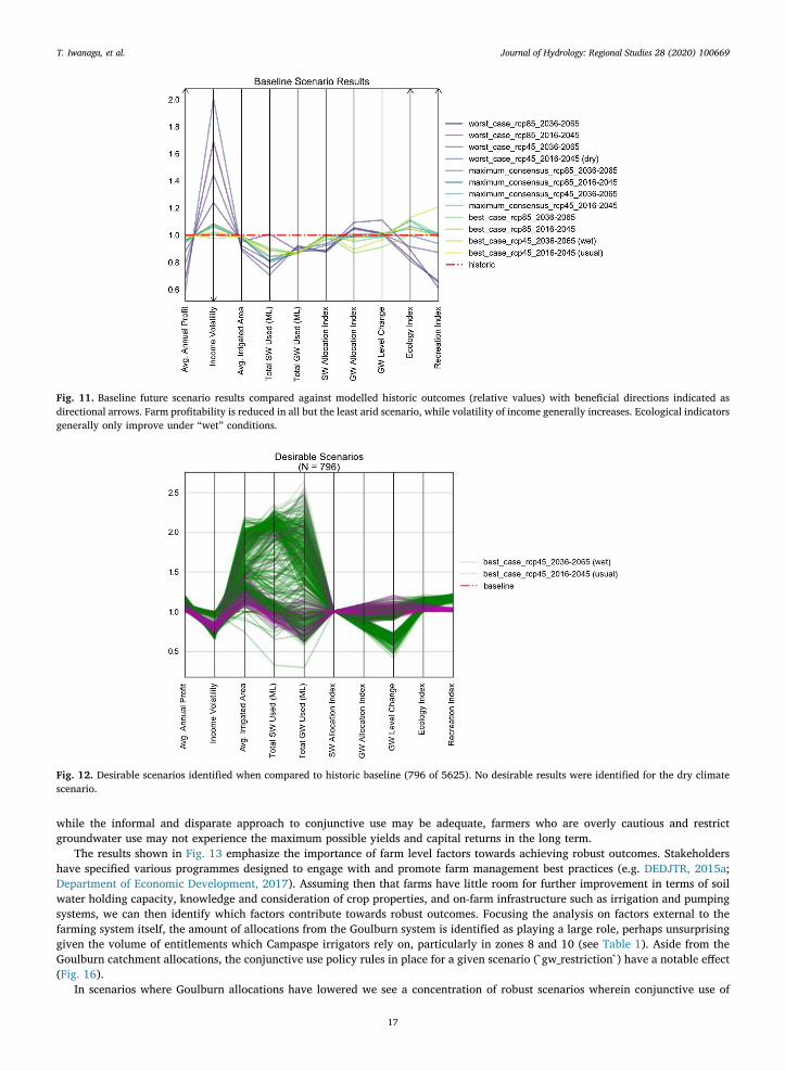
Comparisons of the 5625 scenario results against the historic baseline revealed 796 with desirable outcomes, however none ofthese were robust, i.e. beneficial under all climate conditions, with no desirable outcomes identified under dry climate conditions.

Fig. 7. The six stream gauge locations used to indicate streamflow and level for the Lower Campaspe model. Figure from Iwanaga et al. (2018).


14

The lack of desirable outcomes for the dry climate scenario suggests that improved outcomes compared to historic conditions becomeincreasingly improbable as the climate becomes drier, regardless of what changes are made (Fig. 12). One suggested scenario was theadoption of irrigation systems with higher water application efficiencies to increase water savings across the catchment. Although soilfactors may make such a scenario unlikely (see Section 3.5), no beneficial outcomes were identified in such cases even in the casewhere all non-dryland zones (i.e. all zones except for 1, 3, 5, and 12) adopted improved irrigations.

Given no robust scenarios were identified against historic results, we then conduct comparisons against baseline results forspecific climate conditions. In other words, scenarios under “dry” climate conditions were compared against the “dry” climatebaseline in order to identify conditions that led to relative improvements. A small number of scenarios were identified as being robustunder all climate conditions (93 scenarios). Input parameters of most import leading to these are related to crop, field, and irrigationfactors, followed by policy factors and the maximum amount of groundwater considered. These farm level factors are listed in Table 5(under Section 3.5). The high feature score attributed to crop, field, and irrigation factors is perhaps unsurprising, but it doeshighlight the importance of a well-informed farming community. Over-estimating crop water requirements and costs reduces theirrigation area considered, and poorly set up or poorly maintained irrigation infrastructure (including pumps) and soil health

Fig. 8. Calibrated model compared to observed historic dam level (in mAHD) with an NSE of 0.967. Model parameters were estimated separately foreach of the six segmented time periods indicated with the background colours in the left-hand plot.

Fig. 9. Groundwater model components and model area as well as points and interactions with other component models from the perspective of thegroundwater model. Figure adapted from Iwanaga et al. (2018).


15

increases costs and water usage thereby impacting farm profitability (Fig. 13).At the field level, improving the availability of accurate information on soil water holding capacity has the greatest contribution

to farm profitability. Specifically, soil water retention within Zones 5, 10, and 9 are indicated to influence outcomes more than atother locations in the Lower Campaspe (Fig. 14). At the same time, targeted adoption of spray irrigation within Zones 4 and 9 (thezones indicated to be most amenable to spray irrigation systems in our analysis) did not necessarily lead to robust outcomes, furtherhighlighting the point that simply improving irrigation systems across the catchment is not a viable adaptation strategy. Possiblereasons for this include operational costs incurred with spray irrigation and the lower water efficiency of pipe and riser systemscontributing to increased recharge or streamflow under certain conditions, having the effect of improving ecological outcomes (i.e.due to higher return flows).

One particular aspect of interest was the percentage of groundwater allocation which irrigators consider for use (`gw_cap`,previously explained in Section 3.4.2). While irrigators have historically used 60 % of groundwater allocations in a bid to enhancefuture water security, increased consideration of groundwater use improves the likelihood of desirable outcomes to be experiencedunder all climate conditions (Fig. 15).

Increasing the volume of groundwater to be considered for use compensates for the decreased surface water availability undermore arid conditions. Consideration of all available groundwater resources (100 %) may be necessary under proposed conjunctiveuse rulesets, likely due to the reduction in accessible groundwater in wet periods enforced by the proposed rules. This suggests that

Fig. 10. Modelled catchment average yields produced by CIM under historic climate conditions against available historic data (per farm average forthe North Central region) for the crops considered. The Campaspe region reportedly produces higher yields compared to the North Central average.


16

while the informal and disparate approach to conjunctive use may be adequate, farmers who are overly cautious and restrictgroundwater use may not experience the maximum possible yields and capital returns in the long term.

The results shown in Fig. 13 emphasize the importance of farm level factors towards achieving robust outcomes. Stakeholdershave specified various programmes designed to engage with and promote farm management best practices (e.g. DEDJTR, 2015a;Department of Economic Development, 2017). Assuming then that farms have little room for further improvement in terms of soilwater holding capacity, knowledge and consideration of crop properties, and on-farm infrastructure such as irrigation and pumpingsystems, we can then identify which factors contribute towards robust outcomes. Focusing the analysis on factors external to thefarming system itself, the amount of allocations from the Goulburn system is identified as playing a large role, perhaps unsurprisinggiven the volume of entitlements which Campaspe irrigators rely on, particularly in zones 8 and 10 (see Table 1). Aside from theGoulburn catchment allocations, the conjunctive use policy rules in place for a given scenario (`gw_restriction`) have a notable effect(Fig. 16).

In scenarios where Goulburn allocations have lowered we see a concentration of robust scenarios wherein conjunctive use of

Fig. 11. Baseline future scenario results compared against modelled historic outcomes (relative values) with beneficial directions indicated asdirectional arrows. Farm profitability is reduced in all but the least arid scenario, while volatility of income generally increases. Ecological indicatorsgenerally only improve under “wet” conditions.

Fig. 12. Desirable scenarios identified when compared to historic baseline (796 of 5625). No desirable results were identified for the dry climatescenario.


17

water is allowed. Under median allocation situations, conjunctive use allows robust outcomes to be achieved while maintaininggroundwater use in line with historic behaviour. Without conjunctive use enabled however, considered use of groundwater has toincrease to 90–100% in order for the changes to be robust (Fig. 17). As Goulburn water availability further decreases, groundwateruse becomes especially important towards achieving robust outcomes. Robust outcomes are more likely if conjunctive use is enabledalong with high levels of groundwater use (Fig. 18). The modelling suggests that groundwater levels can be maintained above thelowest trigger level, however careful consideration is required especially with regard to the effect on salinity and water quality issues

Table 5Description of notable farm model inputs.

Factor Name Category Description

gw_cap Direct Control Groundwater cap – described in the policy section above. Reflects maximum volume of groundwater allocationconsidered by a farmer. The farmer may choose to favour future water security under dry conditions by carrying over(25 % of) unused water potentially sacrificing the ability to achieve maximum crop yields in the current season.

irrigation_efficiency Direct Control Irrigation efficiency rating of a given irrigation system. More efficient irrigation systems require less water to irrigatethe same area, but cost more to operate. Efficiency can also be improved by adopting best management practices,which irrigators have been doing.

pumping_costs Direct Control Perceived cost of pumping on a $/kilowatt basis. Farmers can adopt more efficient pumps, irrigation designs, or otherpractices which reduce this cost.

Irrigation Direct Control Indicates adopted irrigation system for a Zonecrop_water_use Limited Control Perceived crop water requirements. Under-estimating crop water requirements leads to too large an irrigated area

relative to available water. Farmers can become better informed of crop attributes but cannot directly control these.crop_root_depth Limited Control Perceived average crop root depth of a crop at each growth stage. Affects irrigation scheduling, as crops with deeper

roots typically require less irrigation events.TAW_mm Limited Control Total Available Water – represents the soil water holding properties of a given soil type. Farmers may improve soils

through best management practices or invest in monitoring but cannot change the soil type at the landscape/fieldlevel.

Table 6Summary of indicator metrics and their beneficial directions. All values should be taken as relative to a baseline, either modelled historic outcomesor a relevant scenario baseline. Indicators provided without a beneficial direction are included to contextualise outcomes, with respect to areairrigated and water used.

Indicator “Beneficial” direction Purpose/Description

Avg. Annual Profit Up General farm profitabilityIncome Volatility Down Severity of fluctuation in profit from year to yearAvg. Irrigated Area – Average total irrigated area over timeTotal SW Used – Comparative surface water useTotal GW Used – Comparative groundwater useSW Allocation Index – Surface water allocations throughout scenario period.GW Allocation Index – Groundwater allocations throughout scenario period.GW Level Change – Averaged normalised change in groundwater level between the start and end of a scenario period.Ecology Index Up Assessment of ecological outcomes of streamflowRecreation Index Up Assessment of impacts of dam levels on recreation

Fig. 13. Robust scenario results (93 of 5625) under all climate conditions. Salient factors leading to robust outcomes include crop, field, andirrigation factors followed by policy factors and the amount of groundwater considered for use.


18

– aspects which the modelling presented here did not cover.The results suggest that improvements to farm soils and infrastructure will be beneficial within the Campaspe, and additional

communication, training, and (financial) incentive programmes beyond what has already been occurring may increase benefits. Anysuch programme should consider possible issues surrounding social acceptability and be cognisant of issues with previous approachesto appraising the cost-benefits (Grafton and Wheeler, 2018). While increasing groundwater use is generally beneficial, possible issuessurrounding social acceptability of increased use and water quality, particularly salinity, should be fully considered. The results raisethe possibility of increasing groundwater allocations in the Lower Campaspe, especially if Managed Aquifer Recharge is adopted inthe region (Chiew et al., 1995; Ticehurst and Curtis, 2017).

5.1. Model and scenario uncertainty

Integrated models are constructed through the interfacing of models that collectively cross disciplinary lines and their respectivesystem boundaries. Intuitively, uncertainty will not decrease if more models are added, simply due to compound uncertainty. This isthe uncertainty that arises as outputs from one model are used as inputs to another, with each interaction propagating some amountof error (Dunford et al., 2015; Refsgaard et al., 2007).

In the context of the CIM the sources of uncertainty and their contributions to total model uncertainty are too great to list outindividually within the confines of this paper. Formal analyses of individual model components and total model uncertainty includingstructural uncertainty with regards to model selection, is the subject of another paper. Qualitatively, however, the farm modelrepresents the largest source of (compound) uncertainty as all components, except for climate, are influenced by mechanisms internalto the farm model. In other words, the farm model behaves as a nexus point between models and thus the errors in the interoperateddata may be cancelled out or compounded and subsequently propagated through. An over estimation of streamflow may be “cor-rected” in a sense by over estimation of required crop water and under estimation of irrigation efficiency. Similarly, the opposite mayalso be true. Such influence may occur directly (e.g. streamflow reduced due to farm water extraction) or indirectly (e.g. ecologicalsuitability influenced by streamflow). The reader is once again referred to Fig. 2 which indicates the component interactions.

Uncertainty within the models was addressed through participatory engagement processes (Section 3.1) and the conceptualtesting process (Section 3.9), both of which ensured model behaviour is qualitatively plausible (as judged by stakeholders), and whichinvolved changes in response to their feedback. On top of this, exploratory modelling was applied to hypothetical policy contextsidentified by stakeholders and the range of on-farm activities considered, using results from the farmer survey (Ticehurst and Curtis,2017, 2016).

Fig. 14. Influence of soil total available water (TAW) towards achieving robust outcomes (shown in log scale).


19

Fig. 15. Number of desirable outcomes experienced under each modelled climate condition. The number of scenarios leading to desirable outcomesincrease as the amount of groundwater considered increases (compared to the historic 60 %).

Fig. 16. Features scores when considering policy factors alone.


20

Each scenario explored was tied to three specific climate datasets which represent hypothetical shifts in aridity (i.e. “dry”, “usual”,and “wet” conditions). Limiting the climate scenarios to these three was done to keep the total number of possible scenario com-binations to a manageable level as model runtime was a concern. An alternate approach is the use of multiple projections for eacharidity scenario. This would more comprehensively address scenario uncertainty with respect to climate inputs as it would allow theinfluence of differing degrees of “dryness” to “wetness” to be explored.

Another source of uncertainty, rarely discussed, is computational infrastructure uncertainty. Here, we define computational infra-structure uncertainty as the uncertainty that arises in model interoperation and integration and application across various compu-tational contexts. Model technical uncertainty (as defined in Refsgaard et al., 2007) is a related issue which we regard as being specificto the uncertainties that may arise from a model’s implementation. Computational infrastructure uncertainty is distinguishable frommodel technical uncertainty in that models that have identical implementations may yet exhibit different behaviour when applied ondifferent infrastructure, such as operating systems (see for example, Bhandari Neupane et al., 2019), platforms (e.g. desktop vssupercomputer), interoperation of data via various means (e.g. local storages vs over a network) and formats and different

Fig. 17. Dimensional stack of current and conjunctive use policies under median Goulburn allocations with respect to considered farm groundwateruse. A concentration of robust outcomes is found in scenarios wherein conjunctive use is allowed with groundwater use levels in line with what hasbeen occurring historically. Without conjunctive use increased groundwater use (to 90–100 %) is necessary to achieve robust outcomes.


21

(programming) languages, or due to the use of different compilers (or different versions of the same compiler).Computational infrastructure uncertainty was addressed by applying the model across various computational infrastructure in-

cluding, but not limited to, both Windows and Linux operating systems, different (Fortran and C) compilers, and ensuring identicalbaseline results. A major error was discovered through this process due to the declaration of an uninitialized variable in the Fortrancode, which was subsequently used in a later calculation. Depending on the compiler, the ‘default’ behaviour may be to initialize theundefined variable to 0.0 (and thereby will have no effect on the result) or may hold ‘junk’ values from its location in memory space,which subsequently propagate throughout the integrated model.

6. Limitations and future work

A difficult aspect to manage in the study was the determination of model scope. The collaborative modelling undertaken en-compasses several disciplinary domains from economics and finance, bio-physical and social aspects and computational considera-tions. Limiting the scope to a manageable size often boiled down to making pragmatic compromises. Here we detail some known

Fig. 18. Dimensional stack of current and conjunctive use policies under low Goulburn allocations. An increase to 90–100 % of groundwater use isnecessary to increase the likelihood of having robust outcomes.


22

limitations and avenues for future work.Climate data used in the modelling display little changes in evapotranspiration from scenario to scenario. Evapotranspiration is

used as a reference value that informs crop water use in the model, and ultimately the frequency of irrigation throughout the growingseason. Crop loss, due to extreme heat, pests, or other influences, are also not considered. Changing weather events due to a changingclimate will also require the growing season to be shifted earlier or later (Prokopy et al., 2015; Wang et al., 2019), or timed to takeadvantage of forecasted rainfall, however these planting/harvest dates were constants in the modelling.

An avenue for further enhancement can be expanding the agricultural activities represented in the model. Dairying is a primaryindustry in the study area but is not explicitly represented in the model. Cropping was determined to be the common agriculturalactivity regardless of farm enterprise and so the decision was made to focus efforts towards representing farm behaviour in thatcontext. While irrigation with groundwater was found to be an important aspect towards yielding robust outcomes, the model did notincorporate water quality aspects and so further in-depth investigation, particularly on salinity issues, are required.

Cropping enterprise profitability may reflect dairying (financial) performance and so beneficial model outcomes are used in thestudy to indicate beneficial outcomes for the catchment generally. As noted by stakeholders, the relationship between the enterprisesis expected to be particularly poor in dry conditions as dairy farmers have the option of acquiring feedstock externally. Irrigators mayalso trade water (an activity not represented in the model) to cover shortfalls in water availability.

Averaging farm water orders across a 14-day time step means that the CIM does not represent high volume water orders that arereleased within a shorter time span. Consequently, the implications of high-volume water orders on ecological flow suitabilityindicator may not be adequately captured. On this note, the policy model currently includes environmental considerations based onlegislated flow requirements but is not reactive to modelled streamflow/level or groundwater head, and effects on ecological in-dicators. Future work could then consider possible adaptive management processes in which water allocations and/or their releasesare adjusted to meet environmental considerations.

Whilst uncertainty in the modelling is taken into account largely through the use of climate scenarios and sampling of parameterspace, future work is envisaged to identify the most important sources of uncertainty in the modelling. In this endeavour, one wayforward is to use a comprehensive qualitative and quantitative approach (e.g. Refsgaard et al., 2007), especially involving stake-holders and experts in helping to rank the criticality of the different sources as to their influence on model outcomes before em-barking on a quantitative set of exercises. Nevertheless, we believe the work to this point is a valuable starting point for raisingawareness and discussion amongst stakeholders as to opportunities for managing water more beneficially in the catchment.

One important social aspect not represented in the presented study is the cultural importance of the local flora and fauna andissues of cultural flows – the release of water to fulfil activities or conditions of cultural and social importance (Moggridge et al.,2019). Indeed, it has been increasingly acknowledged that water entitlements for cultural flows are not yet made a consistent part ofAustralian water management legislation, policies or guidelines despite being identified as a national priority area (Jackson et al.,2012; Williams et al., 2019). This limitation will be addressed in planned future work currently under discussion.

7. Conclusions on sustainable water management opportunities

This paper presents a component-based integrated environmental model developed to explore sustainable water managementoptions within the Lower Campaspe sub-catchment of the Murray-Darling Basin. Stakeholder participation was critical to the modelcapabilities, as local stakeholders provided knowledge, feedback and data to assist in conceptualising the system. The participatoryand model-based collaborative approach yields results that reveal opportunities to consider for achieving improved socio-environ-mental outcomes and water security, relative to the modelled historic baseline. Improvements at the farm level were found to be aprospective contribution towards this goal, as were farm (water) management and changes to governing policy rules. Specifically,conjunctive use of surface and groundwater resources and increased use of the latter was found to improve outcomes. Adoption of themost efficient irrigation systems considered (spray and pipe and riser) did not necessarily lead to desirable outcomes across allclimate conditions. It then follows that simply improving irrigation water efficiency is not a sufficient course of action.

Declaration of Competing Interest

None to declare.

Acknowledgements

The primary author is supported through an Australian Government Research Training Program (AGRTP) Scholarship and a top-up scholarship from the ANU Hilda-John Endowment Fund. The work was carried out as part of the Murray-Darling Basin Authority’spartnership with the National Centre for Groundwater Research and Training (NCGRT). The authors would like to thank re-presentatives from the North Central Catchment Management Authority, the Australian Platypus Conservancy, Goulburn-MurrayWater and the Victorian Department of Economic Development, Jobs, Transport and Resources for their valuable insights and as-sistance over the course of this work. The authors also gratefully thank Joseph Guillaume and Adrian Hindes for comments andsuggestions prior to and throughout the review process, and the anonymous reviewers for their suggestions to improve the quality ofthis paper. The authors would also like to acknowledge and thank Wendy Merritt, Baihua Fu, and Yueqing Xie for early contributionsto the body of work presented.


23

Appendix A. – Key Terms

Term Description

Beneficial change/out-come

Positive change in the indicators Avg. Annual Profit, Ecology Index, GW Level Change, and Recreation Index compared to baseline (i.e.> 1.0). Negative changes to total surface and groundwater volume used (< = 1.0) and to Income Volatility (< 1.0) is preferred.

Desirable outcome Scenarios which exhibit a beneficial change in system state across all indicatorsRobust outcome Scenarios which exhibit desirable outcomes across all climate conditions

Appendix B. – Farm Model Details

The farm model optimised irrigated area and source of water through linear programming, conducted with the OptLang pythonpackage (Jensen et al., 2017) in the form of:

== …

A R Cmaximize , ( )i

i i i1 3

s.t.

==

+

A L L AA AA A A

Rule1.0 if field is dryland onlyRule 2.Rule 3.0

i i i T

T

sw gw f

,

(1)

where A indicates the area to be serviced by each water source, and where i {1,2, 3} represents the water source to be used: sw(surface water), gw (groundwater), or only rainfall (dryland, nw). R is the gross revenue per hectare that can be expected with thecrop (sown for the season), irrigation system, and water source(s),C represents the costs incurred for the same. A is limited (Li) by theavailable water resources and expected crop water demands. In the case of dryland, the total field area can be used (AT). The valuesfor L are calculated asV W/i c ha, as in the volume of available water from a particular water source (Vi) divided by the expected seasonal(per hectare) crop water requirements (Wc ha, ). In future modelling, irrigation areas could be informed based on recent Landsatimagery.

At the start of the season, only Rules 1 and 2 are used to determine the irrigated area for the growing season. The initiallyoptimised area (Af ) is then locked for the rest of the growing season and is used to determine the proportional amount of water to beapplied with surface and groundwater, such that in subsequent time steps Rule 3 is included in the formulation.

Dryland cropping is assumed to occur on non-irrigated areas, the area for which is calculated as = +A A A A( )nw T gw sw . Costsincluded in the calculation include the variable costs for the crop sown, maintenance of irrigation and pumping systems (if ap-plicable), costs associated with licensing, water ordering, and pumping costs. The sum of these gives the dollar profit/income ( ) forthe farm/zone. In this manner the farm costs, expected yields and profit, and estimated crop water requirements play a role inscheduling irrigation events. The estimated total profit is necessarily an approximation. Profit after harvest is calculated directly fromcrop yield, as detailed below.

Irrigation Scheduling

Farmers will irrigate, ideally, when crops require additional water. Determining when these irrigations occur is referred to asirrigation scheduling. In this model it is assumed that farmers are monitoring soil moisture levels and have access to weather data,specifically pan evapotranspiration (ET0). Soil water deficit (SWD) is a cumulative indicator of how dry soils can become beforeadditional water is required to be applied to avoid crop losses. Soil water deficit worsens by subtracting crop evapotranspiration (ETc)which is calculated by applying a scaling crop coefficient Kc (i.e. =ET ET Kc c0 ), with each crop type having a corresponding Kc value.Once SWD reaches a refill point – commonly referred to as the Net Irrigation Depth (NID) – an irrigation event is scheduled and SWDreduced by the effective water applied. This approach is commonly applied on-farm and examples can be found in publications fromState governments (see for example, Hughes, 1999; Qassim and Ashcroft, 2002).

The NID value itself is calculated by multiplying the effective root zone at a point in time (Drz t, ) with the possible ReadilyAvailable Water (RAW ) for the given soil type. The effective root zone is the depth at which the crop gets much of its water via itsroots and is dependent on soil type and crop properties (Baker and Ahern, 1989). Here, Drz is assumed to be 55 % of root depth for thegiven crop type (as in Qassim and Ashcroft, 2002) where relevant information regarding root depths throughout the season and cropgrowth stages could not be obtained, and as such acts as a constant. If sufficient data were available, the alternative approach wouldbe to calculate it as:

=D RD ERDrz t t t, (2)

where RDt is the root depth for the stage of growth at time t , and ERDt the effective root depth coefficient for the crop type(Maihol et al. in Itier et al., 1996). Nominal values for these parameters were obtained from FAO guidelines (Allen et al., 1998).

The Net Irrigation Depth can then be calculated as


24

= =NID D RAW RAW TAW p,t rz t, (3)

Here,TAW corresponds to the Total Amount of Water a soil can hold, and p represents the crop soil water depletion fraction (as inQassim and Ashcroft, 2002). The values used forTAW is discussed in the next section on soils. The soil water deficit at a point in timecan be calculated as:

= +SWD SWD ET E IWmin{ ( ), 0}t t c t t t1 , (4)

where

= =

=E

PP

if month is June to Augustmax{ 5, 0} if other monthst

tn

t

tn

t

1

1and represents the total effective rainfall that occurred within the (two week) time step

(i.e. all winter rainfall is assumed to be effective rainfall)IWt denotes the irrigation water applied at the time step. No water may be applied in the time step in which case this coefficient

will be 0.ETc t, is the sum of crop evapotranspiration (ETc) that occurred within the time step.It should be noted here that the intention of this particular model is not to have an accurate representation of effective rainfall or

water recharge/drainage processes. The model is, as mentioned above, based on the published advice for irrigators in Victoria and sorepresents the assumed behaviour of the irrigation process. Irrigation occurs to refill SWD once it reaches (or goes beyond) NID, andthese are both represented as negative values (or else 0). The base volume of irrigation water (IWb) to be applied is taken to be equalto SWDt when it reaches this refill point. This volume is then adjusted to reflect the efficiency of the implemented irrigation system(IE) to arrive at the amount of irrigation water to be applied (IWt).

= =IWIW

IEIW SWD SWD NID, max{abs( ), 0}t

b tb t t t t

,, (5)

Irrigation efficiency refers to the percentage of water that reaches the crop root zone, allowing the crop ease of access to water.Water applied with less efficient irrigation systems are said to be “lost” for the purpose of contributing to crop growth. Therefore,more water is required if applied with irrigation systems of lesser efficiency for an equivalent effect on SWD. Irrigation systemsconsidered in this study include gravity, pipe and riser, and spray with IE ratings of 0.5, 0.7 and 0.8 respectively. Returning, finally,to the proportional use of irrigation water, Agw sw, (the areas watered by ground and surface water respectively) are each then dividedby Af (total irrigated area) and constrained by the volume of water available. The optimal mix of water sources to use is thenindicated by:

IW AA

V IWA

min , /t

ws

f

t

f (6)

whereV is the volume of available water (in ML), and Aws is the fixed area irrigated by the given water source (e.g. Asw or Agw). Thisprocess (depicted in Fig. 19) is repeated until the crop is harvested at the end of the growing season.

Estimated costs for each irrigation system were corroborated by a senior irrigation specialist with EcoDev (Maskey, 2016). Thesimplest irrigation system is “gravity” which relies on, as the name suggests, gravity to flood an area with water. Pipe and risersystems are similar in that it also ‘floods’ a field but instead uses a pressurized pipe system to transport water, increasing costs. Spray

Fig. 19. Example depiction of irrigation scheduling.


25

is the most efficient but is also the most expensive to install and operate due to the fuel costs necessary to generate the pressureneeded to move and apply water.

The upper limit for all irrigation systems was set to 90 % - which is possible for all systems depending on soil type, system set upand configuration, and additional work conducted to make the field more amenable for the chosen irrigation type (Finger and Morris,2005). For example, the field could be laser graded to ensure a more consistent application of gravity fed irrigation water. Indeed, 77% of those survey respondents reported having undertaken additional improvements to gravity irrigation such as laser grading andtail-water reuse (from excess water reaching the bottom of the field). Gravity irrigation was then modelled as being 50 % and 90 %efficient based on this information with the base efficiency set at 50 % representing the “usual” case (Table 7).

Soils

An early iteration of the model used the dominant soil type found in the Lower Campaspe area (sandy loam, see Fig. 21) as arepresentative surrogate. Stakeholders indicated that this approach may not adequately represent the importance of soil type andhealth in agricultural enterprises due to the diversity found at the smaller (zonal) scales. Stakeholders further indicated that farmerswith lighter soils on their lands may find spray irrigation more attractive as light soils are not capable of holding as much water asheavy soils – the TAW value is comparatively less, influencing irrigation scheduling. Equally true is that farmers with heavier soilsmay not see a benefit from a move to spray. To reflect this, only farm zones that were identified as having light soils were modelled tohave the option of changing irrigation systems to spray irrigation.

To better represent the conditions which impact irrigation scheduling and choice of irrigation system it is then necessary torepresent the range of soil textures within the model farm zones. To achieve this, published TAW value ranges for various soil types(Allen et al., 1998; Qassim and Ashcroft, 2002) were used in conjunction with a soil map of the Campaspe catchment to createweighted zonal values (see Fig. 20). These values were based on the proportional area of soil types found within a zone. A weightedaverage median value was used as the nominal “best guess” value, with the weighted minimum and maximum values indicating thepossible value bounds. The soil map was kindly provided by EcoDev, a Victorian State Government department.

Pumping

Pumping water for irrigation typically represents the largest operational costs for a farm (DEPI 2014a). Seasonal pumping costswere considered as this may vary depending on climate conditions and allocated water availability. This cost can itself vary de-pending on the type of pump and its configuration. Extracting groundwater decreases the groundwater level, thereby increasingpumping costs due to the greater distance and pressure required.

Pumping systems were simplified into two categories, indicating whether they are for shallow or deep bore pumping. The formerrepresents pumping from an irrigation channel or shallow aquifer, with the latter used to represent groundwater pumping at a depthof 20 m or more. Stakeholders indicated that a mix of diesel and electric pumps are used in the study area (60 % and 40 %respectively). Electric pumping costs can range from 16.5c to 32.8c per kilowatt (kW), while electricity plans with a flat rate of 27c/kW can also be arranged (Bob Knowles, 8 Jan 2018, pers. comm). Diesel fuel was assumed to have a cost of $1.20 per litre, with a fuelvolume per kW of 0.25 (Robinson, 2002), resolving to 30c/kW. A weighted average of these values was used to represent the mixed(60 %/40 %) use of both diesel and electric pumps (28.5c/kW). The kW cost of pumping is likely to change over time but wasmodelled as a constant under the assumption that the cost of upgrading infrastructure is cost prohibitive within the modelled timeframe.

Installation of bores to access groundwater incur significant capital costs, ranging from $18,000 to $70,000 for a shallow bore and$90,000 to $320,000 for deep bores (Robinson, 2002). It is assumed here that such infrastructure is already in place and so no initialcapital costs are considered. The average annual maintenance costs are included in the modelling, however, and are taken to be 5 %of capital costs every 5 years and 20 % every 15 years (minor and major maintenance respectively). Nominal values for these (shallowand deep bore) capital costs were $18,000 and $235,000 (taken from Robinson, 2002). The number and location of groundwaterbores for each farm zone are indicated in Fig. 22.

Table 7Implementation costs for each irrigation system considered and their efficiencies.

Variable Irrigation Nominal value (and range) Description Reference(s)

Cost ($/Ha) Dryland $0 (relies on rainfall) Cost of implementation (or replacement) perhectare of irrigated area in AUD ($/Ha)

(Laffan and Smith, 2015)Gravity $2000 ($2000 - $2500)Pipe and Riser $2500 ($2000 - $3000)Spray $2500 ($2500 - $3500)

Irrigation Efficiency (%) Gravity 50 % (50 %–90 %) Expected efficiency for each irrigation system Finger and Morris (2005)Tennakoon et al. (2013)Pipe and Riser 70 % (60 %–90 %)

Spray 80 % (70 %–90 %)


26

Pumping costs throughout the irrigation season is then calculated as

=C C C h( )PML fuel kW ML (7)

Read as the cost per pumped ML being equal to the cost of fuel (per litre) by the cost per kilowatt (kW) hour, multiplied by thehours necessary to pump a megaliter of water. The total pumping cost can then be determined simply as

=C IW Cpump PML (8)

In the presented modelling CkW is calculated in advance (28.5c/kW, as detailed earlier), however it can be calculated directly ifneeded and the necessary information on the pumping system is available. The calculation takes the form of:

Fig. 20. Soil texture map for the Lower Campaspe farm zones with a zoomed close-up of Zone 7 showing the heterogeneity of surface soils. Soil mapwas obtained via EcoDev.

Fig. 21. Area for each soil type for the Lower Campaspe as a whole, and an example Zone (Zone 7 in the above). Sandy loam (soil code “SL”)dominates the catchment area, but variations can be seen within specific Zones, precluding the use of a single representative soil type. A weightedTAW value based on the proportional area for each soil type found in the Zone was used instead.


27

=PUMP P kW F( )fuel (9)

where

=F 0.25

=P kWH f

E D( )

( )(102 )*

c

p

The volume of diesel fuel (PUMPfuel) is based on the required energy (P kW( )) and number of litres required to produce 1 kW( =F 0.25, as given in Robinson, 2002). The amount of kilowatt energy required is dependent on the total head pressure (in metres,H), the flow capacity of the irrigation system in use ( fc), pump efficiency (Ep) and derating factor (D).

Head pressure (H) is defined as the sum of 1) the discharge pressure head, 2) the friction head of water flow (i.e. friction loss) and3) the height between the source of water and the discharge level (Robinson, 2002). The typical total pumping head for a givenirrigation system supplied with surface water is taken from Smith (2015). These values range from 10 m head pressure for gravity to60 m for spray irrigation. Although the values in Smith (2015) are intended for irrigators in New South Wales, the indicated pumpingcosts were within the value range suggested by a local irrigation specialist (Maskey, 2016) for a type of flood irrigation (pipe andriser, $8-15), and spray irrigation system (centre pivot, $30-50). Typical head and cost ranges are shown in Table 8. Head pressure ismultiplied by the flow capacity of the irrigation system ( fc) the value of which is taken from literature regarding a farm in the studyarea, given as 138.88 litres/second, or 12 ML/Day (DEDJTR, 2015). The literature-derived values assume that the pumping systemcan operate at the desired head pressure and flow rate and that the pump itself is in good condition.

Pump efficiency (Ep) is the percent energy efficiency of the pump, representing the amount of energy imparted on the water. This

Fig. 22. Number of bores within each farm zone.


28

value is multiplied by a constant of 102 to convert unit of pressure (kPa) into metres (given in Faour 2001 in Robinson, 2002). Thederating factor (D) accounts for efficiency losses between the total amount of energy required and the energy required at the pumpshaft. The derating factor is said to be 0.75 for diesel pumps (Faour 2001 in Robinson, 2002). As pumping efficiencies may vary modelevaluation was conducted with Ep set to a conservative value of 0.7, the suggested value to use when the pump configuration andefficiency are unknown (Vellotti and Kalogerinis, 2013). Other efficiency losses which influence total pumping head are not explicitlyconsidered but are accounted for through the use of this conservative pump efficiency value (as in Vellotti and Kalogerinis, 2013).

Groundwater pumping costs may fluctuate due to the changes in height distance between water source and discharge pointresulting in an increase in total pumping head. Such a decrease in water levels necessitates increased amounts of energy (and thusfuel) to pump water from the increased distance. To account for decreasing water levels the depth of groundwater is added to thehead values given by Smith (2015) to allow consideration of the effect of fluctuating groundwater levels.

The time taken to pump a single ML of water (hML) is then determined by dividing the number of litres in a ML by the flow rate (Q,in litres per second). This resolves to the number of seconds required to pump 1 ML. Dividing this by the number of seconds in anhour (3600 or 602) results in the hour(s) required to pump 1 ML.

= =hQ

10 /60 , 10 1MLML6

2 6(10)

Crops

The crops represented include three cereal crops of wheat, barley and canola. These are applied as a three-year rotation; i.e.cultivating wheat one year, barley the next, and finally canola after which the rotation is repeated. An earlier version included tomatohowever this crop was removed as its widespread cultivation was described as unrealistic and highly improbable by stakeholders, aswere horticultural crops in general.

Determining Seasonal Profit

Values for the expected revenue (R) and associated production costs (C) for each crop and irrigation type used in Eq. (1) are takenfrom various grey literature sources to determine the optimal irrigation volume throughout the growing season (or the irrigated areain the case of the first time step). Once the growing season has ended, however, a modified French-Schultz equation (Oliver et al.,2009; Whitbread and Hancock, 2008) is used to obtain the final crop yield (Table 9).

= + +Y SSM GSR IW V CWUE(( ) )1000 (11)

The modified French-Schultz equation above takes into account the stored soil water at the start of season (SSM), the effectiverainfall that occurred during the growing season (GSR, which is the sum of Et from Eq. (4)), the sum of any irrigation water applied(IW , which will be 0 for dryland crops), and the crop evaporation coefficient (V ) which represents the required rainfall before a cropwill yield. These are then adjusted by a Crop Water Use Efficiency Index (CWUE) to arrive at the per hectare crop yield (Y ). Theresulting value is then converted to tonnes per hectare by dividing by 1000.

Values for the French-Schultz equation were initially taken from published FAO guidelines (Allen et al., 1998), with SSM assumedto be 30 % of rainfall that occurred over February to April. These were subsequently calibrated against historic (per farm average)crop yield data for the North Central region obtained from the Australian Bureau of Agricultural and Resource Economics (ABARES).

Table 8Typical total head for each irrigation system, adapted from Smith (2015) and adjusted with input from Maskey (2016). Thetypical pumping costs indicated on the right-hand column were used to evaluate the pumping cost model.

Irrigation System Total Head (m) Pumping Cost ($/ML) @ $1.20/L diesel fuel

Gravity 10 - 15 8 - 15Pipe and Riser 10 - 15 8 - 15Spray 25 - 35 30 - 60

Table 9Growth stages for Winter Wheat, the length in days for each stage, and assumed planting date in month and day for each season.

Growth Stage Duration (in days) Crop Coefficient Depletion Fraction Source

Initial 30 0.4 0.6 Allen et al. (1998)Development 140 0.4 0.6Mid-season 40 0.9 0.6Late 30 0.25 0.9Season Length 240 DaysAssumed Plant Date 05-25 (MM-DD) DEDJTR (2015b)


29

The North Central region represents an area significantly larger than the Lower Campaspe sub-catchment, however it is the most(spatially) relevant dataset available.

Calibration used the L-BFGS-B function minimization routine – implemented in the `scipy` Python package (Jones et al., 2001) – toreduce Root Square Mean Error (RMSE). This process achieved results with an overall RMSE of 0.68 and a long-term average yieldcomparable to what has occurred historically; 2.37 t/ha compared to the historic seasonal average of 2.27 t/ha for dryland wheat.The parameters for irrigated crops were adjusted to return higher yields (as is usual for crops under irrigation). The modelled resultswith calibrated values for both dryland and irrigation yields were deemed to be acceptable and reasonable by stakeholders. Furtherexample calibration results are shown in Fig. 23.

The seasonal profit is calculated in the same manner as used to optimize water usage (see Eq. (1)), albeit with yield values (Y )replaced with those calculated by the French-Schultz equation, and the costs now representing the variable and fixed costs associatedwith the cropping enterprise, but also the costs accrued throughout the growing season, such as cost of pumping and water accessfees. From here, the per hectare profit for a growing season ( ha) and profit per ML of water used ( W ) can be determined as:

=Aha

T

T (12)

=Ww

T

T (13)

where WT is the total water volume applied for the season and AT is the earlier defined total field area. Rather than model a globalcrop market, it is assumed here that the harvest for each year is sold.

Appendix C. Representing Goulburn Allocations

See Table 10 Fig. 24.

Fig. 23. Calibrated crop model results for (left to right) dryland and irrigated wheat. Long-term modelled yield was 2.37 t/ha compared to thehistoric average of 2.27 t/ha for dryland. The irrigated crop yields were adjusted to return higher yields compared to dryland production as thehistoric observations are farm averages. The Campaspe catchment is said to produce higher yields than regional averages. Results were deemedacceptable by stakeholders.

Table 10Goulburn allocation scenarios and relationship with Campaspesurface water allocations.

Scenario Equation

High 1.2525x + 48.541Median 1.4005x + 5.3381Low max(0, (1.0116x – 3.2019))


30

Appendix D. Calibration periods for IHACRES rainfall-runoff model

See Table 11.

Appendix E. Ecology and recreation index model detail

Platypus Index

Indicators developed for platypus are based on recommendations outlined in the Environmental Water Management Plan set outby the North Central Catchment Management Authority (North Central CMA, 2014). Following these recommendations streamflow isto be maintained to at least 10 ML/day in the summer, and 50 ML/day in winter to allow for movement and food supply (macro-invertebrate productivity and dispersal). Water releases in the summer and autumn (“freshes”) are necessary to maintain food supplyand, in the autumn, aid in the movement of platypus young. An additional “burrow flooding” index is used to represent prolongedhigh flow events during the nursing season which may flood platypus burrows and drown the young.

Fish Index

Fish represented in the ecology model are categorised by their lifespans (long and short-lived fish). Examples of long-lived fishinclude the Murray Cod and the Golden Perch, with their oldest recorded estimated ages being 48 years (Anderson et al., 1992) and26 years (Mallen‐Cooper and Stuart, 2003) respectively. Short-lived fish include the rainbowfish and carp gudgeons which havetypical lifespans of 2–3 years. Species of long-lived fish have individual spawning preferences, e.g. Murray Cod is considered to spawnin low-flow conditions whereas Golden Perch prefer high-flow flood conditions. In contrast, short-lived fish generally prefer low-flowconditions (Ralph et al., 2010). Fish indicators represent suitable conditions during breeding and nesting seasons (low flow insummer and winter, e.g. 500–1000 ML/day), spring freshes to trigger spawning events for long-lived fish (at least 500 ML/day fortwo days), and summer and autumn freshes for dispersal for long-lived fish (e.g. 50 ML/day for at least two days).

Fig. 24. Linear relationships between Campaspe allocations and allocations in the Goulburn catchment.

Table 11Time span of each period used to calibrate the IHACRES model.

Label Historic Time Span Daily Time Step Index

Pre-drought 1981-01-01 to 1995-03-13 1 – 5185Start-drought 1995-03-14 to 2000-06-13 5186 – 7104Early-drought 2000-06-14 to 2003-04-20 7105 – 8145Mid-drought 2003-04-21 to 2005-11-21 8146 – 9091Late-drought 2005-11-22 to 2010-06-20 9092 – 10763Post-drought 2010-06-21 to 2016-12–31 10764 - End


31

River Red Gum (tree) Index

River red gums play vital roles in the maintenance of the aquatic and riparian ecosystem in the Campaspe River. The modelprovides indications of suitability for maintenance and regeneration (e.g. promotion of new growth) of River Red Gums whichincorporates both groundwater and surface water flow regimes. Suitable groundwater conditions were taken from Roberts andMarston (2011) with established trees preferring the groundwater table to sit between 2 and 6 m below the ground. A linear reductionfrom 6 m to 12 m (where 12 m or more will produce a zero indicator value) is used in the model. Younger trees are modelled to prefergroundwater depths between 0.5 and 1 m, after which the index linearly deteriorates towards 2 m at which point the indicator gives ascore of 0.

Recreation Index

Lake Eppalock is a popular destination for water-related recreational activities including boating, water skiing, and wind surfing,with associated economic benefits (City of Greater Bendigo, 2009). Falling water levels during the millennium drought and in recentyears have led to increased concern for the continued viability of the dam for recreational purposes (ABC News, 2015; City of GreaterBendigo, 2009).

The volume of water in the dam is used to indicate the perceived suitability of the dam for recreational purposes where suffi-ciently high dam levels (> 65 % dam capacity) allows full enjoyment of recreational activities, whereas lower dam levels impedethem. Collision with debris and fallen trees is a risk when the dam falls to 30 % capacity. Issues of crowding can occur at lowervolumes as it equates to lower surface area for recreational use.

Appendix F. – Parameter Covariance Analysis

Fig. 25.

References

ABC News, 2015. Protesters Fear Falling Lake Eppalock Levels. [WWW Document]. ABC News. URL https://www.abc.net.au/news/2015-01-26/protesters-fear-falling-lake-eppalock-levels/6045852 (accessed 10.28.19). .

Allen, R.G., Pereira, L.S., Raes, D., Smith, M., 1998. Chapter 8 - ETc under soil water stress conditions. Crop Evapotranspiration – Guidelines for Computing Crop WaterRequirements, FAO Irrigation and Drainage Paper. Food and Agriculture Organization of the United Nations (FAO).

Fig. 25. Covariance matrix indicating (statistical) independence of model inputs. The number of scenarios to run (896) for each climate scenariowas selected as a compromise between the time taken to run the model and the independence of inputs.


32

http://refhub.elsevier.com/S2214-5818(19)30372-6/sbref0005




Alston, M., Whittenbury, K., 2011. Climate change and water policy in Australia’s irrigation areas: a lost opportunity for a partnership model of governance. Env. Polit.20, 899–917. https://doi.org/10.1080/09644016.2011.617175.

Anderson, J.R., Morison, A.K., Ray, D.J., 1992. Age and growth of Murray Cod, Maccullochella peelii (Perciformes: Percichthyidae), in the Lower Murray-DarlingBasin, Australia, from thin-sectioned Otoliths. Mar. Freshwater Res. 43, 983–1013. https://doi.org/10.1071/mf9920983.

Austin, E.K., Handley, T., Kiem, A.S., Rich, J.L., Lewin, T.J., Askland, H.H., Askarimarnani, S.S., Perkins, D.A., Kelly, B.J., 2018. Drought-related stress among farmers:findings from the australian rural mental health study. Med. J. Aust. 209, 159–165. https://doi.org/10.5694/mja17.01200.

Australian Department of Agriculture, 2019. AGSURF Data - Australian Bureau of Agricultural and Resource Economics and Sciences. [WWW Document]. AgSurfData. URL http://apps.agriculture.gov.au/agsurf/agsurf.asp (accessed 7.10.19). .

Badham, J., Elsawah, S., Guillaume, J.H.A., Hamilton, S.H., Hunt, R.J., Jakeman, A.J., Pierce, S.A., Snow, V.O., Babbar-Sebens, M., Fu, B., Gober, P., Hill, M.C.,Iwanaga, T., Loucks, D.P., Merritt, W.S., Peckham, S.D., Richmond, A.K., Zare, F., Ames, D., Bammer, G., 2019. Effective modeling for Integrated Water ResourceManagement: a guide to contextual practices by phases and steps and future opportunities. Environ. Model. Softw. 116, 40–56. https://doi.org/10.1016/j.envsoft.2019.02.013.

Baker, D.E., Ahern, C.R., 1989. Estimates of effective rooting depth for predicting available water capacity of Burdekin soils, Queensland. Aust. J. Soil Res (Australia).(Queensland D. of P.I.

Bakker, M., Post, V., Langevin, C.D., Hughes, J.D., White, J.T., Starn, J.J., Fienen, M.N., 2016. Scripting MODFLOW Model Development Using Python and FloPy.Groundwater 54, 733–739.

Beverly, C., Hocking, M., 2014. DEPI Northern Victoria Groundwater Model Conceptualisation and Calibration (No. 104220. Department of Environment and PrimaryIndustries with Hocking et al. Pty Ltd, Rutherglen, Victoria, Australia.

Bhandari Neupane, J., Neupane, R.P., Luo, Y., Yoshida, W.Y., Sun, R., Williams, P.G., 2019. Characterization of Leptazolines A–D, Polar Oxazolines from theCyanobacterium Leptolyngbya sp., Reveals a Glitch with the “Willoughby–Hoye” Scripts for Calculating NMR Chemical Shifts. Org. Lett. 21, 8449–8453. https://doi.org/10.1021/acs.orglett.9b03216.

Bowler, M., 2015. Report for the Department of Agriculture and Water Resources - Goulburn-murray Water Connections Project Stage 2 - Mid Term Review (No. 08/08200/07). GHD, Melbourne, Victoria, Australia 2015.

Bruyn, L.A.L., 2019. Learning opportunities: understanding farmers’ soil testing practice through workshop activities to improve extension support for soil healthmanagement. Soil Use Manag. 35, 128–140. https://doi.org/10.1111/sum.12466.

Chiew, F.H.S., McMahon, T.A., O’Neill, I.C., 1992. Estimating groundwater recharge using an integrated surface and groundwater modelling approach. J. Hydrol. 131,151–186. https://doi.org/10.1016/0022-1694(92)90216-I.

Chiew, F.H.S., McMahon, T.A., Dudding, M., Brinkley, A.J., 1995. Technical and economic evaluation of the conjunctive use of surface and groundwater in theCampaspe Valley, north-central Victoria. Australia. Water Resour Manage 9, 251–275. https://doi.org/10.1007/BF00872487.

City of Greater Bendigo, 2009. Rural Areas Strategy. City of Greater Bendigo - Strategy Unit.CSIRO, 2017. Climate Change in Australia [WWW Document]. URL https://www.climatechangeinaustralia.gov.au/en/ (accessed 12.13.17). .DEDJTR, 2015a. Irrigation Supply System Modernisation Enables Farm Irrigation Upgrades. Department of Economic Development, Jobs, Transport and Resources

(DEDJTR), State of Victoria, Tatura, Victoria.DEDJTR, 2015b. Victorian Winter Crop Summary 2015. Department of Economic Development, Jobs, Transport and Resources (DEDJTR), State of Victoria, Tatura,

Victoria, Victoria.Department of Economic Development, J, 2017. Farm Management [WWW Document]. URL http://agriculture.vic.gov.au/agriculture/farm-management (accessed

8.8.19).. .DSE, 2012a. How carryover works on the Murray. Goulburn & Campaspe: Carryover Review Committee fact sheet 1.DSE, 2012b. Limiting Carryover to Your Water Share Volume: Carryover Review Committee Fact Sheet. pp. 3.DSE, 2012c. Victorian Aquifer Framework: Updates for Seamless Mapping of Aquifer Surfaces.Dunford, R., Harrison, P.A., Rounsevell, M.D.A., 2015. Exploring scenario and model uncertainty in cross-sectoral integrated assessment approaches to climate change

impacts. Clim. Change 132, 417–432. https://doi.org/10.1007/s10584-014-1211-3.EcoDev, 2015. Victorian Winter Crop Summary 2015.Elsawah, S., Filatova, T., Jakeman, A.J., Kettner, A.J., Zellner, M.L., Athanasiadis, I.N., Hamilton, S.H., Axtell, R.L., Brown, D.G., Gilligan, J.M., Janssen, M.A.,

Robinson, D.T., Rozenberg, J., Ullah, I.I.T., Lade, S.J., 2020a. Eight Grand Challenges in Socio-environmental Systems Modeling. pp. 16226. https://doi.org/10.18174/sesmo.2020a16226. 16226,1 2.

Finger, L., Morris, M., 2005. Water Management Options: Assisting Irrigators With Stream Flow Management Plan Implementation. Department of Primary Industries(DPI).

Fu, B., 2017. Modelling Ecological Indices to Evaluate Suitability of Surface Water and Groundwater Regimes in the Lower Campaspe: Draft Technical ReportSubmitted to the MDBA-NCGRT Partnership. Available on request. .

Gamo, M., Shinoda, M., Maeda, T., 2013. Classification of arid lands, including soil degradation and irrigated areas, based on vegetation and aridity indices. Int. J.Remote Sens. 34, 6701–6722. https://doi.org/10.1080/01431161.2013.805281.

GHD, 2015. Report for the Department of Agriculture and Water Resources – Goulburn-murray Water Connections Project Stage 2 - Mid Term Review.GM-W, 2013. Lake Eppalock Land and On-Water Management Plan. Tatura, Victoria. .Goode, A.M., Barnett, B.G., 2008. Southern riverine plains groundwater model calibration report. A Report to the Australian Government From the CSIRO Murray-

darling Basin Sustainable Yields Project. CSIRO, Australia.Goulburn-Murray Water, 2015. Lower Campaspe Valley WSPA Annual Report 2015 [WWW Document]. URL https://www.g-mwater.com.au/downloads/gmw/

Groundwater/Lower_Campaspe_Valley_WSPA/30_Sept_2015-LOWER_CAMPASPE_VALLEY_WSPA_ANNUAL_REPORT_-_2014_15_-_SIGNED.pdf (accessed 7.4.19). .Grafton, R.Q., Wheeler, S.A., 2018. Economics of water recovery in the Murray-Darling Basin, Australia. Annual Rev. Res. Eco. 10, 487–510. https://doi.org/10.1146/

annurev-resource-100517-023039.Haasnoot, M., Kwakkel, J.H., Walker, W.E., ter Maat, J., 2013. Dynamic adaptive policy pathways: a method for crafting robust decisions for a deeply uncertain world.

Glob. Environ. Chang. Part A 23, 485–498. https://doi.org/10.1016/j.gloenvcha.2012.12.006.Herman, J.D., Reed, P.M., Zeff, H.B., Characklis, G.W., 2015. How Should Robustness Be Defined for Water Systems Planning under Change? J. Water Resour. Plan.

Manag. 141, 4015012. https://doi.org/10.1061/(ASCE)WR.1943-5452.0000509.Hughes, J.D., 1999. SOILpak - Southern Irrigators | NSW Department of Primary Industries [WWW Document]. URL http://archive.dpi.nsw.gov.au/content/land-

and-natural-resources/soil-management/south-irrig (accessed 4.23.19). .Hughes, L., Steffen, W., Rice, M., Pearce, A., 2015. Feeding a Hungry Nation: Climate Change, Food and Farming in Australia.Itier, B., Maraux, F., Ruelle, P., Deumier, J.M., 1996. Applicability and limitations of irrigation scheduling methods and techniques (No. 8). Irrigation Scheduling: From

Theory to Practice. Food and Agriculture Organization of the United Nations (FAO).Ivkovic, K.M., Croke, B.F.W., Kelly, R.A., 2014. Overcoming the challenges of using a rainfall–runoff model to estimate the impacts of groundwater extraction on low

flows in an ephemeral stream. Nord. Hydrol. 45, 58–72. https://doi.org/10.2166/nh.2013.204.Iwanaga, T., Zare, F., Croke, B., Fu, B., Merritt, W., Partington, D., Ticehurst, J., Jakeman, A., 2018. Development of an integrated model for the campaspe catchment:

a tool to help improve understanding of the interaction between society, policy, farming decision, ecology, hydrology and climate. In: Proceedings of theInternational Association of Hydrological Sciences. Presented at the Innovative Water Resources Management &Ndash; Understanding and Balancing Interactionsbetween Humankind and Nature - 8th International Water Resources Management Conference of ICWRS, Beijing, China, 13-15 June 2018, Copernicus GmbH. pp.1–12. https://doi.org/10.5194/piahs-379-1-2018.

Jackson, S., Tan, P.-L., Mooney, C., Hoverman, S., White, I., 2012. Principles and guidelines for good practice in Indigenous engagement in water planning. J. Hydrol.474, 57–65. https://doi.org/10.1016/j.jhydrol.2011.12.015. Water Planning in Australia: meeting the challenges of incorporating social, cultural and scientificinformation into decision-making.


33

https://doi.org/10.1080/09644016.2011.617175

https://doi.org/10.1071/mf9920983

https://doi.org/10.5694/mja17.01200

http://apps.agriculture.gov.au/agsurf/agsurf.asp

https://doi.org/10.1016/j.envsoft.2019.02.013








https://doi.org/10.1021/acs.orglett.9b03216

https://doi.org/10.1021/acs.orglett.9b03216



https://doi.org/10.1111/sum.12466

https://doi.org/10.1016/0022-1694(92)90216-I

https://doi.org/10.1007/BF00872487


https://www.climatechangeinaustralia.gov.au/en/










https://doi.org/10.1007/s10584-014-1211-3


https://doi.org/10.18174/sesmo.2020a16226

https://doi.org/10.18174/sesmo.2020a16226





https://doi.org/10.1080/01431161.2013.805281





https://www.g-mwater.com.au/downloads/gmw/Groundwater/Lower_Campaspe_Valley_WSPA/30_Sept_2015-LOWER_CAMPASPE_VALLEY_WSPA_ANNUAL_REPORT_-_2014_15_-_SIGNED.pdf

https://www.g-mwater.com.au/downloads/gmw/Groundwater/Lower_Campaspe_Valley_WSPA/30_Sept_2015-LOWER_CAMPASPE_VALLEY_WSPA_ANNUAL_REPORT_-_2014_15_-_SIGNED.pdf

https://doi.org/10.1146/annurev-resource-100517-023039

https://doi.org/10.1146/annurev-resource-100517-023039

https://doi.org/10.1016/j.gloenvcha.2012.12.006

https://doi.org/10.1061/(ASCE)WR.1943-5452.0000509






https://doi.org/10.2166/nh.2013.204

https://doi.org/10.5194/piahs-379-1-2018

https://doi.org/10.1016/j.jhydrol.2011.12.015


Janssen, S., Louhichi, K., Kanellopoulos, A., Zander, P., Flichman, G., Hengsdijk, H., Meuter, E., Andersen, E., Belhouchette, H., Blanco, M., Borkowski, N., Heckelei, T.,Hecker, M., Li, H., Oude Lansink, A., Stokstad, G., Thorne, P., van Keulen, H., van Ittersum, M.K., 2010. A generic bio-economic farm model for environmental andeconomic assessment of agricultural systems. Environ. Manage. 46, 862–877. https://doi.org/10.1007/s00267-010-9588-x.

Jensen, K., Cardoso, J.G.R., Sonnenschein, N., 2017. Optlang: An algebraic modeling language for mathematical optimization [WWW Document]. J. Open SourceSoftw. https://doi.org/10.21105/joss.00139.

Jones, E., Oliphant, T., Peterson, P., et al., 2001. SciPy: Open Source Scientific Tools for Python.Kelly, R.A., Jakeman, A.J., Barreteau, O., Borsuk, M.E., ElSawah, S., Hamilton, S.H., Henriksen, H.J., Kuikka, S., Maier, H.R., Rizzoli, A.E., van Delden, H., Voinov,

A.A., 2013. Selecting among five common modelling approaches for integrated environmental assessment and management. Environ. Model. Softw. 47, 159–181.https://doi.org/10.1016/j.envsoft.2013.05.005.

Kwakkel, J.H., Haasnoot, M., Walker, W.E., 2016. Comparing Robust Decision-Making and Dynamic Adaptive Policy Pathways for model-based decision support underdeep uncertainty. Environ. Model. Softw. 86, 168–183. https://doi.org/10.1016/j.envsoft.2016.09.017.

Laffan, J., Smith, P., 2015. Irrigation: system and pump selection. NSW Agriculture.Letcher, R.A., Croke, B.F.W., Jakeman, A.J., 2007. Integrated assessment modelling for water resource allocation and management: A generalised conceptual fra-

mework. Environmental Modelling & Software, The Implications of Complexity for Integrated Resources 22, 733–742. https://doi.org/10.1016/j.envsoft.2005.12.014.

Mallen‐Cooper, M., Stuart, I.G., 2003. Age, growth and non-flood recruitment of two potamodromous fishes in a large semi-arid/temperate river system. River Res.Appl. 19, 697–719. https://doi.org/10.1002/rra.714.

Maskey, R., 2016. Campaspe - Data Enquiry for Masters Project.McKay, J., 2005. Water instititional reforms in Australia. Water Policy 7, 35–52. https://doi.org/10.1080/02508069908692147.McPhail, C., Maier, H.R., Kwakkel, J.H., Giuliani, M., Castelletti, A., Westra, S., 2018. Robustness Metrics: How Are They Calculated, When Should They Be Used and

Why Do They Give Different Results? Earths Future 6, 169–191. https://doi.org/10.1002/2017EF000649.MDBA, 2012. Sustainable Rivers Audit 2: the Ecological Health of Rivers in the Murray–Darling Basin at the End of the Millennium Drought (2008–2010). Summary.MDBA, 2019. Climate Change and the Murray-darling Basin Plan (No. 09/19). Murray‒Darling Basin Authority. Canberra. .Megdal, S.B., Eden, S., Shamir, E., 2017. Water governance, stakeholder engagement, and sustainable water resources management. Water 9, 190. https://doi.org/10.

3390/w9030190.Mitchell, T.D., 2003. Pattern scaling: an examination of the accuracy of the technique for describing future climates. Clim. Change 60, 217–242. https://doi.org/10.

1023/A:1026035305597.Moggridge, B.J., Betterridge, L., Thompson, R.M., 2019. Integrating Aboriginal cultural values into water planning: a case study from New South Wales, Australia.

Australas. J. Environ. Manag. 26, 273–286. https://doi.org/10.1080/14486563.2019.1650837.Niswonger, R.G., Panday, S., Ibaraki, M., 2011. MODFLOW-NWT, a Newton formulation for MODFLOW-2005. Section A, Groundwater; Book 6 Modeling Techniques.

p. 44.North Central CMA, 2014. Campaspe River Environmental Water Management Plan. North Central Catchment Management Authority, Huntly.NVIRP, 2010. Majority of Campaspe Irrigators to Exit Permanently [WWW Document]. URL https://www.g-mwater.com.au/downloads/gmw/connections/

Communication/Media/MediaReleases2010/Majority_of_Campaspe_irrigators_to_exit_permanently.pdf (accessed 2.26.18). .NVIRP, 2011. NVIRP Annual Report 2010-2011.Oliver, Y.M., Robertson, M.J., Stone, P.J., Whitbread, A., 2009. Improving estimates of water-limited yield of wheat by accounting for soil type and within-season

rainfall. Crop Pasture Sci. 60, 1137–1146. https://doi.org/10.1071/CP09122.Peckham, S.D., Hutton, E.W.H., Norris, B., 2013. A component-based approach to integrated modeling in the geosciences: the design of CSDMS. Computers &

Geosciences, Modeling for Environmental Change 53, 3–12. https://doi.org/10.1016/j.cageo.2012.04.002.Prokopy, L.S., Arbuckle, J.G., Barnes, A.P., Haden, V.R., Hogan, A., Niles, M.T., Tyndall, J., 2015. Farmers and climate change: a cross-national comparison of beliefs

and risk perceptions in high-income countries. Environ. Manage. 56, 492–504. https://doi.org/10.1007/s00267-015-0504-2.Pulido-Velazquez, D., Garrote, L., Andreu, J., Martin-Carrasco, F.-J., Iglesias, A., 2011. A methodology to diagnose the effect of climate change and to identify adaptive

strategies to reduce its impacts in conjunctive-use systems at basin scale. J. Hydrol. 405, 110–122. https://doi.org/10.1016/j.jhydrol.2011.05.014.Qassim, A., Ashcroft, B., 2002. Estimating Vegetable Crop Water Use [WWW Document]. Agriculture Victoria. URL http://agriculture.vic.gov.au/agriculture/

horticulture/vegetables/vegetable-growing-and-management/estimating-vegetable-crop-water-use (accessed 4.23.19). .Ralph, T., Spencer, J., Rayner, T., 2010. Chapter 4: Fish. In: Rogers, K., Ralph, T. (Eds.), Floodplain Wetland Biota in the Murray-Darling Basin. CSIRO Publishing.Refsgaard, J.C., van der Sluijs, J.P., Højberg, A.L., Vanrolleghem, P.A., 2007. Uncertainty in the environmental modelling process – a framework and guidance.

Environ. Model. Softw. 22, 1543–1556. https://doi.org/10.1016/j.envsoft.2007.02.004.Reichert, P., Borsuk, M.E., 2005. Does high forecast uncertainty preclude effective decision support? Environmental Modelling & Software. Methods of Uncertainty

Treatment in Environmental Models 20, 991–1001. https://doi.org/10.1016/j.envsoft.2004.10.005.Roberts, J., Marston, F., 2011. Water regime for wetland and floodplain plants: a source book for the Murray-Darling Basin. National Water Commission, Canberra.Robinson, D.W., 2002. Construction and operating costs of groundwater pumps for irrigation in the riverine Plain. CSIRO Land and Water Technical Report. CSIRO

Land and Water, Canberra.Sahin, S., 2012. An aridity index defined by precipitation and specific humidity. J. Hydrol. 444–445, 199–208. https://doi.org/10.1016/j.jhydrol.2012.04.019.Schlüter, M., Haider, L., Lade, S., Lindkvist, E., Martin, R., Orach, K., Wijermans, N., Folke, C., 2019. Capturing emergent phenomena in social-ecological systems: an

analytical framework. Ecol. Soc. 24. https://doi.org/10.5751/ES-11012-240311.Smith, P., 2015. Is Your Diesel Pump Costing You Money?.Steffen, W., Vertessy, R., Dean, A., Hughes, L., Bambrick, H., Gergis, J., Rice, M., 2018. Deluge & Drought: Water Security in a Changing Climate. Climate Council of

Australia.Storn, R., Price, K., 1997. Differential evolution – a simple and efficient heuristic for global optimization over continuous spaces. J. Glob. Optim. 11, 341–359. https://

doi.org/10.1023/A:1008202821328.Suzuki, S., Stern, D., Manzocchi, T., 2015. Using association rule mining and High-dimensional visualization to explore the impact of geological features on dynamic

flow behavior. In: Presented at the SPE Annual Technical Conference and Exhibition. Society of Petroleum Engineers. https://doi.org/10.2118/174774-MS.Tennakoon, S., Richards, D., Milroy, S., Harris, G., 2013. Water use efficiency in the Australian cotton industry, in: Waterpak: A Guide for Irrigation Management in

Cotton and Grain Farming Systems. Cotton Research and Development Corporation 22–27.Ticehurst, J., Curtis, A., 2016. Improving On-farm Water Use Efficiency Amongst Irrigators in the Campaspe River System and the Rochester Irrigation Area. Wagga

Wagga, NSW, Australia 2650.Ticehurst, J., Curtis, A., 2017. Preliminary Assessment of Conjunctive Use Opportunities for in the Murray Darling Basin: a Case Study in the Lower Campaspe

Catchment. Charles Sturt University, Wagga Wagga, NSW 2650.van Dijk, A.I.J.M., Beck, H.E., Crosbie, R.S., de Jeu, R.A.M., Liu, Y.Y., Podger, G.M., Timbal, B., Viney, N.R., 2013v. The Millennium Drought in southeast Australia

(2001–2009): Natural and human causes and implications for water resources, ecosystems, economy, and society. Water Resour. Res. 49, 1040–1057. https://doi.org/10.1002/wrcr.20123.

Vaze, J., Teng, J., Chiew, F.H.S., 2011. Assessment of GCM simulations of annual and seasonal rainfall and daily rainfall distribution across south-east Australia.Hydrol. Process. 25, 1486–1497. https://doi.org/10.1002/hyp.7916.

Vellotti, G., Kalogerinis, K., 2013. Calculating Energy Requirements of Irrigation Systems.Voinov, A., Shugart, H.H., 2013. “Integronsters”, integral and integrated modeling. Environ. Model. Softw. 39, 149–158. https://doi.org/10.1016/j.envsoft.2012.05.

014.Wang, B., Feng, P., Chen, C., Liu, D.L., Waters, C., Yu, Q., 2019. Designing wheat ideotypes to cope with future changing climate in South-Eastern Australia. Agric. Syst.

170, 9–18. https://doi.org/10.1016/j.agsy.2018.12.005.


34

https://doi.org/10.1007/s00267-010-9588-x

https://doi.org/10.21105/joss.00139







https://doi.org/10.1002/rra.714


https://doi.org/10.1080/02508069908692147

https://doi.org/10.1002/2017EF000649



https://doi.org/10.3390/w9030190

https://doi.org/10.3390/w9030190

https://doi.org/10.1023/A:1026035305597

https://doi.org/10.1023/A:1026035305597

https://doi.org/10.1080/14486563.2019.1650837







https://doi.org/10.1071/CP09122

https://doi.org/10.1016/j.cageo.2012.04.002

https://doi.org/10.1007/s00267-015-0504-2











https://doi.org/10.5751/ES-11012-240311




https://doi.org/10.1023/A:1008202821328

https://doi.org/10.1023/A:1008202821328

https://doi.org/10.2118/174774-MS







https://doi.org/10.1002/wrcr.20123

https://doi.org/10.1002/wrcr.20123

https://doi.org/10.1002/hyp.7916




https://doi.org/10.1016/j.agsy.2018.12.005

Wheeler, S.A., Cheeseman, J., 2013. Key Findings from a Survey of Sellers to the Restoring the Balance Programme. Economic Papers 32, 340–352. https://doi.org/10.1111/1759-3441.12038.

Whitbread, A., Hancock, J., 2008. Estimating grain yield with the French and schultz approaches vs simulating attainable yield with APSIM on the eyre peninsula. In:Australian Agronomy Conference. Presented at the 14th Australian Agronomy Conference, Adelaide, South Australia.

Williams, S., Connolly, D., Williams, A., 2019. The recognition of cultural water requirements in the montane rivers of the Snowy Mountains, Australia. Australas. J.Environ. Manag. 26, 255–272. https://doi.org/10.1080/14486563.2019.1652211.

Wines, M., 2015. Protesters voice water concerns [WWW document]. Bendigo Advertiser. URL https://www.bendigoadvertiser.com.au/story/2838129/protesters-voice-water-concerns/ (accessed 10.28.19).

Xie, Y., Crosbie, R., Simmons, C.T., Cook, P.G., Zhang, L., 2019. Uncertainty assessment of spatial-scale groundwater recharge estimated from unsaturated flowmodelling. Hydrogeol. J. 27, 379–393. https://doi.org/10.1007/s10040-018-1840-0.


35

https://doi.org/10.1111/1759-3441.12038

https://doi.org/10.1111/1759-3441.12038



https://doi.org/10.1080/14486563.2019.1652211



https://doi.org/10.1007/s10040-018-1840-0

journal of hydrology: regional studies - research @ flinders

Documents