buku forest hydrology (minghteh chang) english sub
TRANSCRIPT


Forest hydrology: An introduction to water and forests
1363_ FM_fm Page 1 Tuesday, December 3, 2002 6:57 AM

1363_ FM_fm Page 2 Tuesday, December 3, 2002 6:57 AM

Forest hydrology: An introduction to water and forests
Mingteh Chang
1363_ FM_fm Page 3 Tuesday, December 3, 2002 6:57 AM

This book contains information obtained from authentic and highly regarded sources. Reprinted material is quoted withpermission, and sources are indicated. A wide variety of references are listed. Reasonable efforts have been made to publishreliable data and information, but the author and the publisher cannot assume responsibility for the validity of all materialsor for the consequences of their use.
Neither this book nor any part may be reproduced or transmitted in any form or by any means, electronic or mechanical,including photocopying, microfilming, and recording, or by any information storage or retrieval system, without priorpermission in writing from the publisher.
The consent of CRC Press LLC does not extend to copying for general distribution, for promotion, for creating new works,or for resale. Specific permission must be obtained in writing from CRC Press LLC for such copying.
Direct all inquiries to CRC Press LLC, 2000 N.W. Corporate Blvd., Boca Raton, Florida 33431.
Trademark Notice:
Product or corporate names may be trademarks or registered trademarks, and are used only foridentification and explanation, without intent to infringe.
Visit the CRC Press Web site at www.crcpress.com
© 2003 by CRC Press LLC
No claim to original U.S. Government worksInternational Standard Book Number 0-8493-1363-5
Library of Congress Card Number 2002023354Printed in the United States of America 1 2 3 4 5 6 7 8 9 0
Printed on acid-free paper
Library of Congress Cataloging-in-Publication Data
Chang, Mingteh.Forest hydrology: an introduction to water and forests
p. cm.Includes bibliographical references and index.ISBN 0-8493-1363-5 (alk. paper)1. Hydrology, Forest. I. Title.
GB842 .C535 2002551.48'0915'2—dc21 2002023354 CIP
1363_ FM_fm Page 4 Tuesday, December 3, 2002 6:57 AM

The rivers run into the sea but the sea is never full, and the water returns again to the rivers, and flows again to the sea.
Ecclesiastes 1:7The Old Testament
1363_ FM_fm Page 5 Tuesday, December 3, 2002 6:57 AM

1363_ FM_fm Page 6 Tuesday, December 3, 2002 6:57 AM
Preface
This book is based on lecture material in the course "Forest Hydrology," offered to under-graduate and postgraduate students in the Arthur Temper College of Forestry at StephenF. Austin State University, Texas. As is the case with many other forestry programs in theU.S., forest hydrology (or watershed management) is the only required course in watersciences in the curriculum. Because students are new to the subject, it is necessary to coversome basic topics in water and water resources before discussing topics in forest hydrology.
Although a few texts on forest hydrology are available for college students, they coververy little or none of the background on water resources. On the other hand, books dealingwith water resources do not cover topics in forest–water relations. This book intends tofill that gap and provide an introduction to forest hydrology by bringing water resourcesand forest–water relations into a single volume, and broadly discussing issues that arecommon to both. It focuses on concepts, processes, and general principles; hydrologicanalyses are not emphasized here.
The book comprises 12 chapters and 3 appendices. Subjects in the 12 chapters arearranged in two general groups. The first six chapters deal with the introduction and basicbackground in water and water resources, while the remaining six chapters address theimpact of forests on water. Chapter 7 describes forests and forest characteristics importantto water circulation and sediment movement. It serves as an introduction to the study offorest impacts on water resources — as a bridge connecting water and forests.
The impacts — precipitation, vaporization, streamflow, and stream sediment — offorests on the hydrologic cycle are discussed separately in Chapters 8 through 11. Stream-flow topics include water quantity, water quality, and stream habitat, while stream sedi-ment topics include erosion processes, sediment predictions, and forest impacts. Thestream habitat section in Chapter 10 (“Forests and streamflow”) was not originallyincluded in this book. Its inclusion is due to the suggestion of Dr. Younes Alila of theUniversity of British Columbia and the increasing interest among forest hydrologists inaquatic environment in relation to the fish population, especially in the Pacific Northwest.Also, sediment predictions are becoming a management tool for controlling nonpointsources of water pollution in forested watersheds. Basic prediction concepts andapproaches are included in the text too. The chapters on streamflow and stream sedimentare therefore much longer than the chapters on precipitation and vaporization.
Chapter 12 deals with forest-hydrology research. It covers research issues, objectives,principles, and methodology along with a step-by-step numerical example of watershedcalibration and assessment of treatment effects. The laborious presentation in Chapter 12provides a foundation for those who might pursue graduate studies or engage in water-shed research.
The book’s discussion of hydrologic measurements covers only precipitation, stream-flow, and stream sediments. Subjects for each type of measurement include general back-ground, available instruments, and sampling procedures. They are presented in the appen-dices for those who practice hydrology in the field.
1363_ FM_fm Page 7 Tuesday, December 3, 2002 6:57 AM

The use of mathematical expressions is inevitable in hydrology and other earth sci-ences. This book uses mathematical equations in forms for which a knowledge of collegealgebra and trigonometry is sufficient for understanding. Readers with less mathematicalbackground can skip the difficult equations without hindering their comprehension. Thebook can be used as a text for students in agriculture, forestry, and land-resources man-agement, and as a reference for foresters, rangers, geographers, watershed managers,biologists, agriculturists, environmentalists, policy makers, engineers, and others who mayneed such background in their professions.
Mingteh Chang
1363_ FM_fm Page 8 Tuesday, December 3, 2002 6:57 AM
Acknowledgments
I am much obliged to Stephen Fuller Austin State University for the award of a sabbaticalleave spring semester 2001 to complete this book. The support of Dr. R. Scott Beasley,dean of the College of Forestry, during my sabbatical leave is gratefully acknowledged.Critical reviews of selected chapters were provided by Drs. Scott Beasley, Douglas G.Boyer, Thomas O. Callaway, Dean Coble, George G. Ice, Ernest Ledger, James A. Lynch,Darrel L. McDonald, Ahmad A. Nuruddin, David A. Rutherford, Donald J. Turton, WilliamE. Sharpe, Kim L. Wong, Lizhu Wang, and Jimmy Williams. Their corrections and sugges-tions have greatly improved the readability, clarity, and contents of the final manuscript.Drs. Mason D. Bryant, John M. Laflen, Kenneth Farrish, David Kulhavy, Shiyou Li, andBrian Oswald provided literature information and other assistance. Matthew McBroomwas the first instructor to use the rough draft of the manuscript in a senior class. Hisexperience with this book and the students in his class provided useful perspective.
Mark C. Cochran of the Texas Soil and Water Conservation Board proofread the entiremanuscript with exceptional care. He also called my attention to a number of issues andprovided new references that are important to forestry students. Mian Ahmad enthusias-tically helped me with a literature search, graphics, files, and computer programs. BrentBishop, Misti Compton, Richard Ford, James Hoard, Danny McMahon, Adam G. Mouton,and Melissa Watson provided assistance with drafting, computer files, a literature search,proofreading, and table preparation. The entire CRC editorial staff, including, but notlimited to, John Sulzycki (senior editor), Judith S. Kamin (project editor), Jamie B. Sigal(production coordinator), and Kristina M. Rosello (editorial assistant), provided assistanceand numerous suggestions. Their professionalism and helpfulness made the completionof this book project smooth and orderly. My children Benjamin, Rebecca, and Solomonalso helped with some computer programs, proofreading, and pictures. Finally, the loveand encouragement of my wife Phyllis were indispensable in the preparation of themanuscript. This book could not have been completed without the support, assistance,and encouragement of the aforementioned individuals. I am very grateful and indebtedto all of them.
I am also grateful to the following organizations, individuals, and publishers forpermission to reproduce copyrighted materials: American Water Resources Association;American Society of Agricultural Engineers; Harwood Academic Publishers; John Wiley& Sons, Ltd.; Springer-Verlag; GmbH & Co. KG; and UNSECO Press.
1363_ FM_fm Page 9 Tuesday, December 3, 2002 6:57 AM

1363_ FM_fm Page 10 Tuesday, December 3, 2002 6:57 AM

Author
Dr. Mingteh Chang
is Regents professor of forest hydrology at theArthur Temple College of Forestry, Stephen F. Austin State Uni-versity in Nacogdoches, Texas. He has taught courses there onforest hydrology, watershed management, environmental mea-surements, hydrologic measurements, hydrologic analyses, micro-climate, forest soils, and introduction to forestry at the undergrad-uate and graduate levels since 1975.
Dr. Chang was born in China and grew up in Taiwan. Heworked for 3 years as watershed technologist for the Taiwan pro-vincial government and for 2 years as a laboratory lecturer at
National Chung-Shing University, Taichung, Taiwan before he started his graduate workat Pennsylvania State University and West Virginia University. He is a certified profes-sional hydrologist and a member of the American Water Resources Association, AmericanGeophysical Union, International Association of Hydrological Science, the Soil and WaterConservation Society of America, and the Texas Forestry Association. His major interestsin research are forest–water relations, conservation plants, nonpoint water pollution,precipitation hydrology, and forest climatology. Dr. Chang has four patents and hasauthored or co-authored more than 80 technical articles and three books.
1363_ FM_fm Page 11 Tuesday, December 3, 2002 6:57 AM

1363_ FM_fm Page 12 Tuesday, December 3, 2002 6:57 AM
Contents
Chapter 1 Introduction..............................................................................................................1
Chapter 2 Functions of water ..................................................................................................5
Chapter 3 Water as a science .................................................................................................23
Chapter 4 Properties of water................................................................................................37
Chapter 5 Water distribution .................................................................................................57
Chapter 6 Water resource problems .....................................................................................73
Chapter 7 Characteristic forests...........................................................................................109
Chapter 8 Forests and precipitation ...................................................................................131
Chapter 9 Forests and vaporization....................................................................................151
Chapter 10 Forests and streamflow ......................................................................................175
Chapter 11 Forests and stream sediment.............................................................................233
Chapter 12 Research in forest hydrology ............................................................................279
Appendix A Precipitation measurements ..............................................................................307
Appendix B Streamflow measurements.................................................................................319
Appendix C Measurements of stream sediment ..................................................................341
Index..............................................................................................................................................361
1363_ FM_fm Page 13 Tuesday, December 3, 2002 6:57 AM

1363_ FM_fm Page 14 Tuesday, December 3, 2002 6:57 AM

1
chapter one
Introduction
Contents
I. Water spectrum....................................................................................................................1II. Forest spectrum ...................................................................................................................2
III. Issues and perspective........................................................................................................3References .........................................................................................................................................4
Water and forests are two of the most important resources on earth. They both providefood, energy, habitat, and many other biological, chemical, physical, and socioeconomicfunctions and services to lives and the environment. Without water, there would be noforests. With forests, the occurrence, distribution, and circulation of water are modified,the quality of water is enhanced, and the timing of flow is altered. Indeed, water andforests impact each other greatly.
I. Water spectrum
Water is essential to life, the environment, and human development. Flora and faunadepend on water for growth, development, and survival, and water sustains humansocieties; environments without water are hot, dry, uncomfortable, and unsuitable forliving. Fortunately, the Earth is blessed with water. More than 70% of Earth’s surface iscovered by water, and a layer of water vapor up to about 90 km thick embraces the entireplanet. Water makes Earth flourish with lives of various forms and with places for culturesto develop.
Although water on Earth is so abundant in quantity and so vast in distribution, it stillimposes problems in many regions. At least 80 countries, accounting for nearly 40% ofthe world’s population, have experienced periodic shortages of water preventing themfrom growing enough food to support their people (Miller, 1999). Water-pollution prob-lems have made the regions with water shortages even worse. Water shortage not onlycreates many problems and inconveniences in daily activities, but also affects lifestylesand cultural development. At Chungungo, Chile, each villager lived on 13 liters of waterper day delivered by trucks once a week. In the northwest plateau of China, it is said thatpeople take only three baths in their lifetimes: when they are born, when they are married,and when they die. Indeed, water is a luxury to many people in many regions.
On the other hand, many people in other parts of the world suffer damage, casualties,and life disruptions from disastrous floods. A major flood occurred in the upper Missis-sippi and lower Missouri rivers in the summer of 1993. The flood affected nine states in
1363_C01_fm Page 1 Tuesday, December 3, 2002 6:58 AM
2 Forest Hydrology: An Introduction to Water and Forests
which more than 41,000 km
2
of farmland and 75 small towns were completely under waterfor months. Property damages were estimated to exceed $20 billion (Dvorchak, 1993).Probably the most devastating flood in modern times was the Yellow River (Huang Ho)flood in China, which occurred between July and November 1931. It completely inundated87,000 km
2
, partially inundated another 20,000 km
2
, drowned 1 million people, and left80 million people homeless (Clark, 1982).
Since water is so crucial to life, livestock are grazed in areas with plenty of water andgrass, crops are grown along floodplains, cities are built along major rivers and seaports,and civilizations are developed in regions with mild climates and an abundance of waterresources. The Nile River has thus been referred to as the “Springs of Life” and the YellowRiver as the “Cradle of Chinese Civilization.” However, the uneven distribution of wateron Earth has caused major disputes over water throughout history and in modern times,between nations, within countries, and among people.
Wars over water between nations were fought in the Mideast throughout ancienthistory and continue even today. Babylon, for example, was a center of dispersal ofagricultural knowledge in early historical times, about 5000 years ago. Babylonia occupiedthe lower delta of the Tigris and Euphrates Rivers, which was exceptionally fertile becauseof alluvial deposits from Assyrian highlands and the retreat of the great ice sheet. Theconstant wars for water supply between Babylonia and Assyria partially contributed tothe fall of Babylonian civilization.
In the U.S., the 19th-century California gold rush produced diverse competition forwater between farmers and miners, between cattle grazers and crop growers, and betweenadvocates of both public and private irrigation (Pisani, 1992). The availability and distri-bution of water is a determining factor for the prosperity of cities, industries, agriculture,and tourism in the Western region of the U.S., where water scarcity is a common phenom-enon. A dam on the Nueces River Basin in south Texas was planned in the 1960s but wasdelayed for almost 20 years due to disputes over water rights between upstream anddownstream water users, along with the conceptual struggle between conservationistsand developers. Allocating freshwater inflows from the Nueces River to bays and estuariesfor maintaining a healthy and productive Texas estuarine system created a series ofconflicts among the Fish and Wildlife Service, the Bureau of Land Reclamation, TexasWater Commission, and the City of Corpus Christi, Texas, as well as between environ-mental groups and individuals (Ting, 1989).
Indeed, water is a major concern in our society. People are concerned with too muchwater, too little water, water being unsafe to use, no rights to use water, and waterallocation. Most universities provide training on subjects relating to water. For example,all 16 state-controlled four-year universities in Texas offer courses related to water. Knowl-edge of water properties, problems, environmental significance, and management is essen-tial for effective utilization of this vital natural resource.
II. Forest spectrum
A forest is a biotic community predominated by trees and woody vegetation that cover alarge area. It supports an array of complex flora and fauna. The forest forms a distinctivemicroclimate compared to other land uses. Of the many different types of forests, eachhas different characteristics such as species composition, size, diversity, and density, withvariation depending mainly on temperature and precipitation. No matter what type theforest is, the plant sizes, canopy density, litter floor, and root systems are significantlytaller, greater, thicker, and deeper than other vegetation types. These characteristics makeforests able not only to provide a number of natural resources, but also to perform avariety of environmental functions.
1363_C01_fm Page 2 Tuesday, December 3, 2002 6:58 AM
Chapter one: Introduction 3
Resources associated with forests may include timber, water, soil, wildlife, vegetation,minerals, and recreation. Except for minerals, all these resources are greatly affected byforestry activities. Some resources can be completely destroyed, depending on the intensityand extent of the forest activity. Environmental functions performed by forests may includecontrol of water and wind erosion, protection of headwater and reservoir watershed andriparian zone, sand-dune and stream-bank stabilization, landslide and avalanche preven-tion, preservation of wildlife habitats and gene pools, mitigation of flood damage andwind speed, and sinks for atmospheric carbon dioxide. Many established forests havemanaged to achieve one or more of these environmental functions, while others arepreserved to prevent reduction in biodiversity and degradation of the ecosystem.
The approximately 4.2
¥
10
9
ha of forests and woodlands on Earth cover about one-third of the total land surface. This is about 80% of the preagriculture forested areas(Mather, 1990). Forested areas in the Temperate Zone (23.5 to 66.5
∞
latitudes) have notchanged much in recent decades, but deforestation in the tropical regions was conductedat about 17
¥
10
6
ha/year in the 1980s and is believed to have been done at least the sameamount in the 1990s. Tropical forests make up about one-half of the world’s forest cover(World Resources Institute, 1996) and are the major genetic and pharmaceutical pools ofthe world. Judging from the forest environmental functions mentioned above, the impactsof such large-scale forest destruction on soil, water, air, and biology have been of greatconcern among scientists, environmentalists, policy makers, and the general public.
History and modern studies have shown that the misuse of forest resources has causedadverse watershed conditions, depletion of land productivity, disruption of people’s rou-tine activities, conversion of arable lands into semiarid or desert, and destruction ofvillages, towns, or even civilizations. Through these experiences, the use of forests hasbeen shifted from single into multiple purposes — from exploitative into preservation andthen conservation uses, and from productive into environmental and then ecologicalfunctions. The recent growing interest in biological sinks of atmospheric carbon dioxide,global warming, and the balance between production and protection are examples of theawareness of ecological functions. It is our task to seek a balance in forest managementbetween productive and protective functions.
III. Issues and perspective
Water and forests both cover large portions of Earth and both are crucial to lives and theenvironment. As the world’s population exponentially increases with time, so do thepressures of population and the extent of utilization of all natural resources. This makeswater and forests two of the most important issues in the 21st century. We are concernedwith water and forests not only as raw materials required by cultures and industries, butalso as key factors in the environment. Water and forests are not two independent naturalresources; a close linkage exists between the two. Consequently, a study of the interfacebetween these two resources, called forest hydrology, has become an important field. Itprovides basic knowledge and foundations for watershed management, a discipline andskill for maintaining land productivity and protecting water resources.
Forest distributions enhance the forest–water relation significantly. Forests usuallygrow and develop in areas with annual precipitation of 500 mm or higher. These are alsothe areas suitable for certain agricultural activities. Forests cover about 30% of the land,yet this 30% forested land generates 60% of total runoff. In other words, most of ourdrinking-water supplies originate from forested areas. Any activities, development, andutilization in forested areas will inevitably destroy forest canopies and disturb forest floorsto a certain degree. This may affect water quantity through their impacts on transpirationand canopy interception losses, infiltration rate, water-holding capacity, and overland flow
1363_C01_fm Page 3 Tuesday, December 3, 2002 6:58 AM
4 Forest Hydrology: An Introduction to Water and Forests
velocity. Water quality also is affected because of the exposure of mineral soils to directraindrop impacts, the loss of soil-binding effect from the root systems, the increase inoverland flow, and the accelerated decomposition of organic matter. All these may resultin an increase in soil erosion and nutrient losses. All forests should be managed with theirimpacts on water resource in mind so that water resource can be properly protected andutilized.
Many issues concern water and forests, but this book will emphasize the linkagesbetween the two, beginning with a basic explanation of water and water resources, andthen moving forward to examine the impacts of forests and forest activities. We all rec-ognize that proper management of these two resources is of utmost importance to thewell-being of nations. Without fundamental knowledge, adequate studies, and sufficientinformation, proper management cannot be achieved.
References
Clark, C., 1982,
Flood
, Time-Life, Chicago, IL.Dvorchak, R.J., 1993,
The Flood of ’93
, Wieser & Wieser, New York.Mather, A.S., 1990,
Global Forest Resources
, Timber Press, Portland, OR.Miller, G.T., Jr., 1999,
Environmental Science: Working with the Earth
, Wadsworth, Belmont, CA.Pisani, D.J., 1992,
To Reclaim a Divided West: Water, Law, and Public Policy
, 1848–1902, University ofNew Mexico Press, Albuquerque, NM.
Ting, J. C., 1989, Conflict Analysis of Allocating Freshwater Inflows to Bay and Esturaries — A CaseStudy on Choke Canyon Dam and Reservoir, Texas, Doctoral dissertation, Stephen F. AustinState University, Nacogdoches, TX.
World Resources Institute, 1996,
World Resources
, 1996–97, Oxford University Press, Oxford.
1363_C01_fm Page 4 Tuesday, December 3, 2002 6:58 AM

5
chapter two
Functions of water
Contents
I. Biological functions.............................................................................................................6A. A necessity of life........................................................................................................6B. A habitat of life ...........................................................................................................6
1. Wetlands .................................................................................................................62. Estuaries .................................................................................................................73. Ponds and lakes ....................................................................................................74. Streams and rivers ................................................................................................85. Oceans.....................................................................................................................8
C. A therapy for illness (hydrotherapy).......................................................................8II. Chemical functions .............................................................................................................9
A. A solvent of substance ...............................................................................................9B. A medium in chemical reactions..............................................................................9
III. Physical functions ...............................................................................................................9A. A moderator of climate..............................................................................................9B. An agent of destruction ...........................................................................................10C. A potential form of energy and power.................................................................10D. A scientific standard for properties .......................................................................12E. A medium of transport ............................................................................................13
IV. Socioeconomic functions..................................................................................................13A. A source of comfort ..................................................................................................13B. An inspiration of creativity.....................................................................................14C. An issue of world peace and regional stability...................................................14
1. Regional conflicts ................................................................................................14a. Alabama, Florida, and Georgia ..................................................................15b. Northern vs. Southern California ..............................................................15c. New Mexico vs. Surrounding States .........................................................15d. Eastern vs. Western Colorado.....................................................................15e. Nebraska vs. Wyoming................................................................................15
2. International conflicts.........................................................................................15a. The Euphrates and Tigris ............................................................................15b. The Golan Heights........................................................................................16c. The Nile River ...............................................................................................16d. The Rio Grande .............................................................................................17
D. A medium for agricultural and industrial productions.....................................171. Hydroponics ........................................................................................................18
1363_C02_fm Page 5 Tuesday, December 3, 2002 6:59 AM
6 Forest Hydrology: An Introduction to Water and Forests
2. Fish culture ....................................................................................................193. A tool for industrial operations..................................................................19
References .......................................................................................................................................20
The significance of water to life and the environment can be discussed from the perspectiveof its various biological, chemical, physical, and socioeconomic functions. These functionsstem from its unique properties, abundant quantity, and vast distribution on Earth, whichsubsequent chapters will discuss.
I. Biological functions
A. A necessity of life
Life cannot exist without water; it began in water and depends on water for survival,growth, and development. Water is the primary constituent of protoplasm, a substancethat performs basic life functions. Without water, a plant cannot absorb required nutrients,cannot perform photosynthesis and hydrolytic processes, and cannot maintain its state ofvigor. In animals, water removes impurities and the byproducts of metabolism, transportsoxygen and carbon dioxide, enhances digestion, and regulates body temperature. It actsas a solvent and as a raw material in the chemical reactions necessary to sustain life andmaintains a balance between bases and acids in the body. The tissue can die with minutechanges in pH.
A forest can transpire 1000 kg m
-
2
year
-
1
of water while producing 1 kg m
-
2
year
-
1
ofdry matter. The body of a newborn calf is 75 to 80% water, and 75% of the weight of aliving tree is either water or made from water. Water represents 60 to 90% of human bodyweight. Total daily requirement of water for a person is about 20 liters for minimumcomfort, while 1 to 5 liters are essential for survival. The human body obtains 47% of itswater from drinking, 39% from solid food, and 14% as a by-product of the chemical processof cellular respiration (Leopold and Davis, 1972). We die when 15% of the water in ourbody is lost through dehydration. Man can survive without food for about one to twoweeks, but only a few days without water.
B. A habitat of life
Water is not only the substance of life; it also provides a living environment for about 90%of Earth’s organisms. Blue whales (measured up to 30 m long and 200 t) and hippopota-mus, the two largest mammals on the earth, use oceans and rivers, respectively, as theirhomes. Oceans, seas, streams, rivers, lakes, ponds, estuaries, wetlands, and even bodiesof water in drainage ditches and abandoned containers are habitats to a variety of animalsand plants.
1. Wetlands
Wetlands — areas where water is near, at, or above ground level — are considered to betransitional zones between terrestrial and aquatic ecosystems. The five recognized wetlandsystems are marine, estuarine, lacustrine (associated with lakes), riverine (along riversand streams), and palustrine (marshes, swamps, and bogs). Biologically, they are one ofthe richest and most interesting ecosystems on Earth. Hydrologically, they provide mech-anisms and resources for aquifer recharge, flood control, sediment control, wastewatertreatment, biogeochemical cycling and storage, and water supplies. Richardson (1994)
1363_C02_fm Page 6 Tuesday, December 3, 2002 6:59 AM
Chapter two: Functions of water 7
assigned 5 wetland functions and 19 wetland values only realized in recent decades.Unfortunately, wetlands in the U.S. have reduced more than 50% in the past 200 years.
In the 1780s, there were 89
¥
10
6
ha of wetlands in the conterminous U.S., and wetlandsoccupied 5% or more of the land area in 34 states. By the 1980s, wetlands had decreased53% to 42
¥
10
6
ha, and the number of states that had wetlands on 5% or more of the landarea had fallen to 19 (Dahl, 1990). The losses of wetlands were due to the cumulativeimpact of agricultural development, urban development, conversion of wetlands to deep-water habitats, and other types of conversion activities (Dahl and Johnson, 1991).
2. Estuaries
An estuary is the narrow zone along a coastline where freshwater from rivers mixes witha salty ocean. Estuaries receive heavy loads of sediments, suspended and dissolved organicor inorganic materials, and freshwater from rivers, which provide nutrients and maintainsalinity levels necessary to sustain marine organisms. These distinctive properties, alongwith relatively shallow depths that allow deep penetration of sunlight, make estuariesprimary spawning areas for a wide variety of finfish and shellfish, nurseries for juvenilemarine species, and homes for wildlife and waterfowl (Ting, 1989).
3. Ponds and lakes
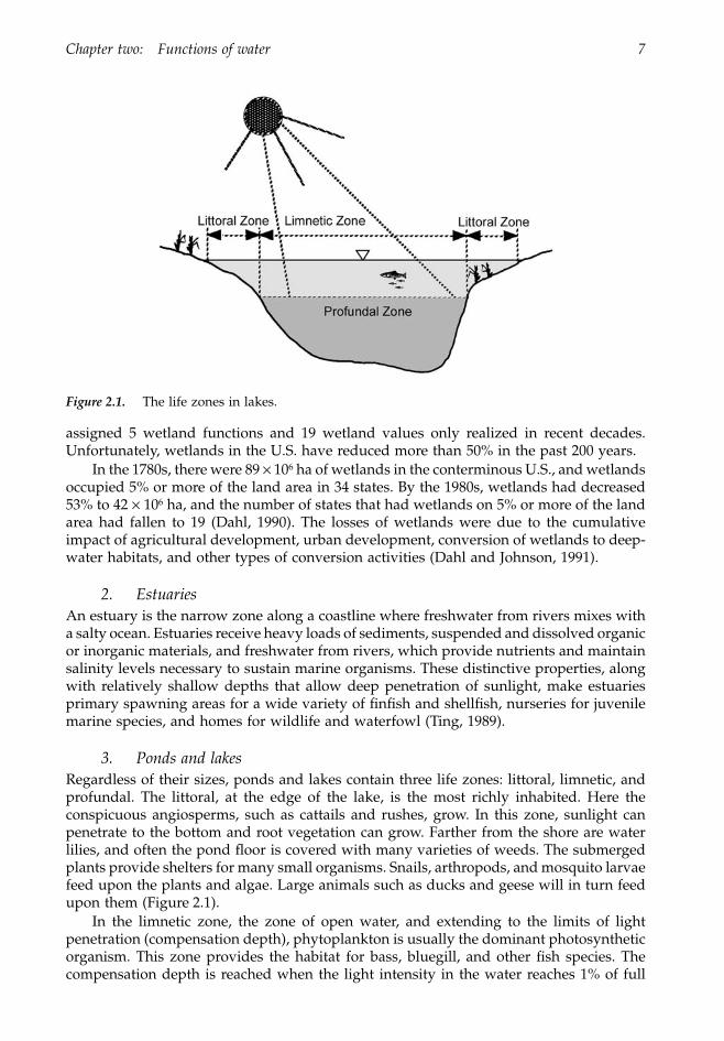
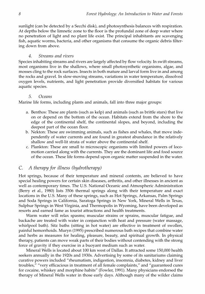
Regardless of their sizes, ponds and lakes contain three life zones: littoral, limnetic, andprofundal. The littoral, at the edge of the lake, is the most richly inhabited. Here theconspicuous angiosperms, such as cattails and rushes, grow. In this zone, sunlight canpenetrate to the bottom and root vegetation can grow. Farther from the shore are waterlilies, and often the pond floor is covered with many varieties of weeds. The submergedplants provide shelters for many small organisms. Snails, arthropods, and mosquito larvaefeed upon the plants and algae. Large animals such as ducks and geese will in turn feedupon them (Figure 2.1).
In the limnetic zone, the zone of open water, and extending to the limits of lightpenetration (compensation depth), phytoplankton is usually the dominant photosyntheticorganism. This zone provides the habitat for bass, bluegill, and other fish species. Thecompensation depth is reached when the light intensity in the water reaches 1% of full
Figure 2.1.
The life zones in lakes.
1363_C02_fm Page 7 Tuesday, December 3, 2002 6:59 AM
8 Forest Hydrology: An Introduction to Water and Forests
sunlight (can be detected by a Secchi disk), and photosynthesis balances with respiration.At depths below the limnetic zone to the floor is the profundal zone of deep water whereno penetration of light and no plant life exist. The principal inhabitants are scavengingfish, aquatic worms, bacteria, and other organisms that consume the organic debris filter-ing down from above.
4. Streams and rivers
Species inhabiting streams and rivers are largely affected by flow velocity. In swift streams,most organisms live in the shallows, where small photosynthetic organisms, algae, andmosses cling to the rock surfaces. Insects in both mature and larval form live in and amongthe rocks and gravel. In slow-moving streams, variations in water temperature, dissolvedoxygen levels, nutrients, and light penetration provide diversified habitats for variousaquatic species.
5. Oceans
Marine life forms, including plants and animals, fall into three major groups:
a. Benthos: These are plants (such as kelp) and animals (such as brittle stars) that liveon or depend on the bottom of the ocean. Habitats extend from the shore to theedge of the continental shelf, the continental slopes, and beyond, including thedeepest part of the ocean floor.
b. Nekton: These are swimming animals, such as fishes and whales, that move inde-pendently of water currents and are found in greatest abundance in the relativelyshallow and well-lit strata of water above the continental shelf.
c. Plankton: These are small to microscopic organisms with limited powers of loco-motion carried along with the currents. They are the dominant life and food sourceof the ocean. These life forms depend upon organic matter suspended in the water.
C. A therapy for illness (hydrotherapy)
Hot springs, because of their temperature and mineral contents, are believed to havespecial healing powers for certain skin diseases, arthritis, and other illnesses in ancient aswell as contemporary times. The U.S. National Oceanic and Atmospheric Administration(Berry et al., 1980) lists 3506 thermal springs along with their temperature and exactlocations in the U.S. Many of these springs, such as Hot Springs, Arkansas, Palm Springsand Soda Springs in California, Saratoga Springs in New York, Mineral Wells in Texas,Sulphur Springs in West Virginia, and Thermopolis in Wyoming, have been developed asresorts and earned fame as tourist attractions and health treatments.
Warm water will relax spasms; muscular strains or sprains, muscular fatigue, andbackache are treated with water in conjunction with heat and pressure (water massage,whirlpool bath). Sitz baths (sitting in hot water) are effective in treatment of swollen,painful hemorrhoids. Muryn (1995) prescribed numerous bath recipes that combine waterand herbs as measures for healing, pleasure, beauty, and spiritual growth. In physicaltherapy, patients can move weak parts of their bodies without contending with the strongforce of gravity if they exercise in a buoyant medium such as water.
Mineral Wells is located about 100 km west of Dallas. It attracted some 150,000 healthseekers annually in the 1920s and 1930s. Advertising by some of its sanitariums claimingcurative powers included “rheumatism, indigestion, insomnia, diabetes, kidney and livertroubles,” “very efficacious in treatment of all female complaints,” and “guaranteed curesfor cocaine, whiskey and morphine habits” (Fowler, 1991). Many physicians endorsed thetherapy of Mineral Wells water in those early days. Although many of the wilder claims
1363_C02_fm Page 8 Tuesday, December 3, 2002 6:59 AM

Chapter two: Functions of water 9
began fading out due to the invention of antibiotics and advancement of medical sciencein the 1950s, the physical effects of hot springs on blood circulation and tension releasethat everybody can enjoy conveniently and cheaply at home will never meet with substi-tutes in the future.
II. Chemical functions
A. A solvent of substance
Water molecules are covalently bonded together with one oxygen atom and two muchsmaller hydrogen atoms. However, the two hydrogen atoms are separated from eachother on one side at an angle of 105
∞
. As a result, the side with the two hydrogens iselectropositive and the other is electronegative.
The positive (hydrogen) end causes water molecules to attract (cohere) the negative(oxygen) end of another molecule, causing water molecules to join together in chains andsheets that give water a higher viscosity and greater surface tension. Both positive andnegative charges make water molecules attract (adhere) to other materials, which causewater to dissolve a larger variety of substances than any other liquid. Thus, water is thebest cleansing agent for humans, animals, and the environment.
In time, water will dissolve almost any inorganic substance, and about half of theknown elements are found dissolved in water. One liter of water can dissolve 8.4 kg ofthe fertilizer ammonium nitrate (Leopold and Davis, 1972).
B. A medium in chemical reactions
The majority of chemical reactions take place in aqueous solutions, which affect thechemical properties of many materials. For example, pure water contains dissociated H
+
and OH
-
ions in very low concentrations. This makes the pH of materials change whenthey go into solution in water. Water affects chemicals through the processes of hydrolysis,hydration, and dissolution. Hydrolysis is the process that occurs when water enters intoreactions with compounds and ions, while hydration is the attachment of water to acompound. Dissolution refers to the decomposition of ionic compounds in water. Theseprocesses result in degradation, alteration, and resynthesis of minerals and materials.
III. Physical functions
A. A moderator of climate
Atmospheric water vapor absorbs and reflects parts of incoming solar radiation duringthe daytime and provides heat energy to Earth in the form of longwave radiation at night.Moreover, water is a good medium for heat storage when air temperature is high, andthe stored heat in the water is released when the air temperature is low. This is due to thehigh thermal capacity and latent heat of water. Consequently, temperature fluctuationsare always smaller over water than land, and climates in areas close to oceans or lakesare always moderate compared to climates of inland areas. If water vapor were not presentin the atmosphere, Earth’s temperature would be much warmer in the daytime and muchcolder at night.
The Great Lakes region of the U. S. illustrates the effects of water on climate. Theamount of precipitation, and the frequency of thunderstorm and hailstorm activity overthe lakes and their downwind areas, tend to decrease in the summer and increase in thefall and winter (Changnon and Jones, 1972). Apparently, this is because the waters of these
1363_C02_fm Page 9 Tuesday, December 3, 2002 6:59 AM
10 Forest Hydrology: An Introduction to Water and Forests
lakes in the fall and winter are warmer than the overlying air. Precipitation over the lakesand their downwind areas is enhanced when moisture and heat are added from the lakesto increase atmospheric instability. On the other hand, the lakes are cooler than theoverlying air in summer, tending to stabilize the atmosphere, and precipitation is reduced.
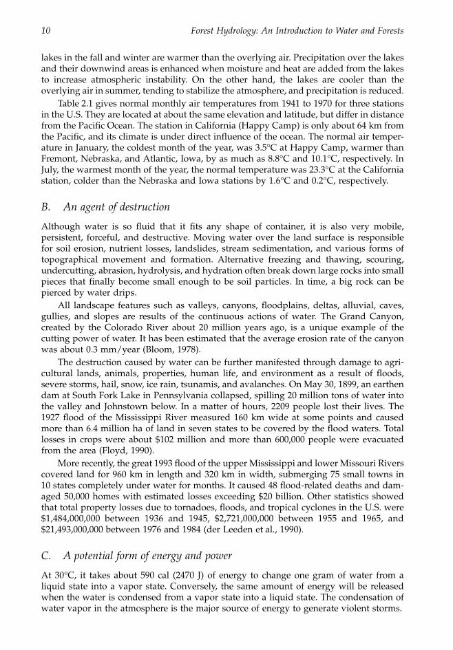
Table 2.1 gives normal monthly air temperatures from 1941 to 1970 for three stationsin the U.S. They are located at about the same elevation and latitude, but differ in distancefrom the Pacific Ocean. The station in California (Happy Camp) is only about 64 km fromthe Pacific, and its climate is under direct influence of the ocean. The normal air temper-ature in January, the coldest month of the year, was 3.5
∞
C at Happy Camp, warmer thanFremont, Nebraska, and Atlantic, Iowa, by as much as 8.8
∞
C and 10.1
∞
C, respectively. InJuly, the warmest month of the year, the normal temperature was 23.3
∞
C at the Californiastation, colder than the Nebraska and Iowa stations by 1.6
∞
C and 0.2
∞
C, respectively.
B. An agent of destruction
Although water is so fluid that it fits any shape of container, it is also very mobile,persistent, forceful, and destructive. Moving water over the land surface is responsiblefor soil erosion, nutrient losses, landslides, stream sedimentation, and various forms oftopographical movement and formation. Alternative freezing and thawing, scouring,undercutting, abrasion, hydrolysis, and hydration often break down large rocks into smallpieces that finally become small enough to be soil particles. In time, a big rock can bepierced by water drips.
All landscape features such as valleys, canyons, floodplains, deltas, alluvial, caves,gullies, and slopes are results of the continuous actions of water. The Grand Canyon,created by the Colorado River about 20 million years ago, is a unique example of thecutting power of water. It has been estimated that the average erosion rate of the canyonwas about 0.3 mm/year (Bloom, 1978).
The destruction caused by water can be further manifested through damage to agri-cultural lands, animals, properties, human life, and environment as a result of floods,severe storms, hail, snow, ice rain, tsunamis, and avalanches. On May 30, 1899, an earthendam at South Fork Lake in Pennsylvania collapsed, spilling 20 million tons of water intothe valley and Johnstown below. In a matter of hours, 2209 people lost their lives. The1927 flood of the Mississippi River measured 160 km wide at some points and causedmore than 6.4 million ha of land in seven states to be covered by the flood waters. Totallosses in crops were about $102 million and more than 600,000 people were evacuatedfrom the area (Floyd, 1990).
More recently, the great 1993 flood of the upper Mississippi and lower Missouri Riverscovered land for 960 km in length and 320 km in width, submerging 75 small towns in10 states completely under water for months. It caused 48 flood-related deaths and dam-aged 50,000 homes with estimated losses exceeding $20 billion. Other statistics showedthat total property losses due to tornadoes, floods, and tropical cyclones in the U.S. were$1,484,000,000 between 1936 and 1945, $2,721,000,000 between 1955 and 1965, and$21,493,000,000 between 1976 and 1984 (der Leeden et al., 1990).
C. A potential form of energy and power
At 30
∞
C, it takes about 590 cal (2470 J) of energy to change one gram of water from aliquid state into a vapor state. Conversely, the same amount of energy will be releasedwhen the water is condensed from a vapor state into a liquid state. The condensation ofwater vapor in the atmosphere is the major source of energy to generate violent storms.
1363_C02_fm Page 10 Tuesday, December 3, 2002 6:59 AM

Chapter two: Functions of water 11
Tabl
e 2.
1
Nor
mal
(19
41–1
970)
Mon
thly
Air
Tem
pera
ture
s fo
r T
hree
U.S
. Sta
tion
s L
ocat
ed a
t ab
out
the
Sam
e E
leva
tion
and
Lat
itud
e bu
t at
Diff
eren
t D
ista
nces
fro
m t
he P
acifi
c O
cean
Ele
vati
on(m
) L
atit
ude
(°)
Jan
Feb
Mar
Apr
May
Jun
Jul
Aug
Sep
Oct
Nov
Dec
Hap
py
Cam
p R
ange
r S
tati
on, C
alif
orn
ia
369
41.4
83.
56.
68.
611
.815
.719
.323
.322
.319
.313
.67.
94.
6
Frem
ont,
Neb
rask
a
366
41.2
6–5
.3–2
.32.
711
.117
.122
.124
.924
.118
.813
.14.
2
-
2.4
Atl
anti
c 1
NE
, Iow
a
364
41.2
5–6
.6–3
.71.
59.
916
.020
.923
.522
.617
.612
.03.
1
-
3.6
Sour
ce:
U.S
. Nat
iona
l Wea
ther
Ser
vice
, Clim
atol
ogic
al D
ata
Ann
ual S
umm
ary,
Cal
ifor
nia,
Neb
rask
a, a
nd I
owa,
197
5.
1363_C02_fm Page 11 Tuesday, December 3, 2002 6:59 AM
12 Forest Hydrology: An Introduction to Water and Forests
Humans have used water as a prime mechanical power for thousands of years. Onesuch use was the water mill. At a water mill, a dam was built across a river, which raisedthe water level. Water spilling over the dam provided force to turn a paddle wheel; itsshaft drove a millstone for grinding grain.
Electricity is the key to success in industrial societies. It provides power to heat andcool buildings, drive trains, melt metals, and run machines. Water helps generate powerthrough thermoelectric and hydroelectric processes. Thermoelectric plants convert waterinto steam by heating it with fossil or nuclear fuels. Hydroelectric power can be generatedusing hydraulic drop in rivers (hydropower), ocean waves (tidal power), or temperaturegradient between surface and deep tropical water (sea thermal power). In the U.S., onlyabout 28% of the maximum potential capacity of hydroelectric power has been developed,which accounts for about 15% of the total electricity produced.
In hydroelectric power, the force used to drive turbines is the “head” of water heldback behind the dam along a river. Total head is the difference in elevation between theturbine and the water level above the turbine. The greater the head is, the more powergenerated in a given amount of water.
The energy created by the head of water in the river can be applied to generate energyin the ocean. Oceanic tides occur as a result of the gravitational attraction in water bodiesof Earth by the sun and moon. Twice a day a tremendous volume of water flows into andout of bays, producing high or low tides. The kinetic energy in the tidal flows, if differencesin water elevation between high and low tides are sufficiently high, can be used to spinturbines to generate electricity. For such purposes, a dam is built, similar to that in a river,with operational gates across the bay. About two dozen sites around the world are suitablefor tidal power generation and dam construction (Miller, 1999).
Caterpillar Inc., a construction and earth-moving equipment manufacturer at Peoria,Illinois, is developing a water-based fuel called A-55. The fuel is a blend of water, carbon-based fuels, and an emulsifier holding the mixture together. Water content in the fuel isexhausted as steam in the combustion process. Initial tests show that A-55 makes the filthyemissions of diesel engines cleaner, reduces emissions, and improves fuel economy. Thecost savings of the fuel are roughly equal to its 55% water content (
U.S. Water News
, 1996a).
D. A scientific standard for properties
Because of its abundance and distribution on the earth, along with its unique physicaland chemical properties, water is used as a scientific standard for mass, specific gravity,heat, specific heat, temperature, and viscosity of other substances.
One kilogram is the mass of water that is free of air at 3.98
∞
C in a volume of 1 literor 1000 g. The ratio between the weight of a given volume of substance and the weightof an equal volume of water is defined as specific gravity. A standard heat unit is expressedin calories. One calorie is defined as the heat required to raise the temperature of 1 g ofliquid water 1
∞
C. The number of calories required to raise 1 g of a substance is definedas the thermal capacity of that substance, and the ratio between the thermal capacity ofa substance and the thermal capacity of water is called specific heat. A typical soil has aspecific heat of 0.25 cal/g/
∞
C, which is about one-fourth that of water. Temperature scales are based on melting ice and boiling water under standard atmo-
spheric pressure. Four temperature scales are in general use today: Fahrenheit (
∞
F), Rank-ine (
∞
R), Centigrade (
∞
C), and Kelvin or Absolute (
∞
K). The temperature of melting ice isset at 32
∞
F, 492
∞
R, 0
∞
C, and 273.16
∞
K, and boiling water is set at 212
∞
F, 672
∞
R, 100
∞
C, and373.16
∞
K. In the U.S., the Fahrenheit scale is commonly used, with the Rankine scale usedmainly by engineers. The Centigrade and Kelvin scales are used internationally for scien-tific measurements.
1363_C02_fm Page 12 Tuesday, December 3, 2002 6:59 AM
Chapter two: Functions of water 13
E. A medium of transport
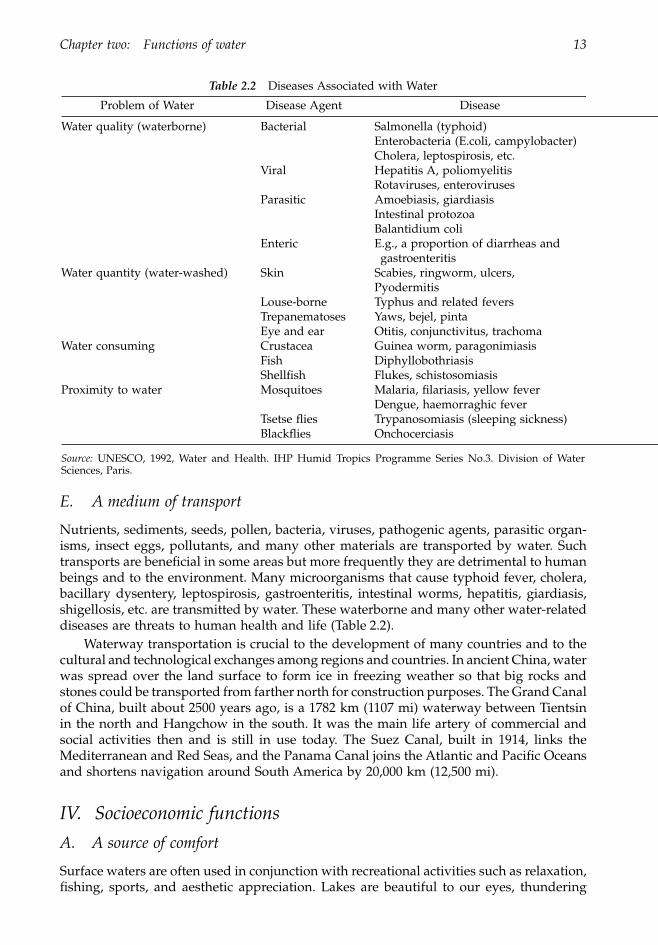
Nutrients, sediments, seeds, pollen, bacteria, viruses, pathogenic agents, parasitic organ-isms, insect eggs, pollutants, and many other materials are transported by water. Suchtransports are beneficial in some areas but more frequently they are detrimental to humanbeings and to the environment. Many microorganisms that cause typhoid fever, cholera,bacillary dysentery, leptospirosis, gastroenteritis, intestinal worms, hepatitis, giardiasis,shigellosis, etc. are transmitted by water. These waterborne and many other water-relateddiseases are threats to human health and life (Table 2.2).
Waterway transportation is crucial to the development of many countries and to thecultural and technological exchanges among regions and countries. In ancient China, waterwas spread over the land surface to form ice in freezing weather so that big rocks andstones could be transported from farther north for construction purposes. The Grand Canalof China, built about 2500 years ago, is a 1782 km (1107 mi) waterway between Tientsinin the north and Hangchow in the south. It was the main life artery of commercial andsocial activities then and is still in use today. The Suez Canal, built in 1914, links theMediterranean and Red Seas, and the Panama Canal joins the Atlantic and Pacific Oceansand shortens navigation around South America by 20,000 km (12,500 mi).
IV. Socioeconomic functions
A. A source of comfort
Surface waters are often used in conjunction with recreational activities such as relaxation,fishing, sports, and aesthetic appreciation. Lakes are beautiful to our eyes, thundering
Table 2.2
Diseases Associated with Water
Problem of Water Disease Agent Disease
Water quality (waterborne) Bacterial Salmonella (typhoid)Enterobacteria (E.coli, campylobacter)Cholera, leptospirosis, etc.
Viral Hepatitis A, poliomyelitisRotaviruses, enteroviruses
Parasitic Amoebiasis, giardiasisIntestinal protozoaBalantidium coli
Enteric E.g., a proportion of diarrheas and gastroenteritis
Water quantity (water-washed) Skin Scabies, ringworm, ulcers,Pyodermitis
Louse-borne Typhus and related feversTrepanematoses Yaws, bejel, pintaEye and ear Otitis, conjunctivitus, trachoma
Water consuming Crustacea Guinea worm, paragonimiasisFish DiphyllobothriasisShellfish Flukes, schistosomiasis
Proximity to water Mosquitoes Malaria, filariasis, yellow feverDengue, haemorraghic fever
Tsetse flies Trypanosomiasis (sleeping sickness)Blackflies Onchocerciasis
Source:
UNESCO, 1992, Water and Health. IHP Humid Tropics Programme Series No.3. Division of WaterSciences, Paris.
1363_C02_fm Page 13 Tuesday, December 3, 2002 6:59 AM
14 Forest Hydrology: An Introduction to Water and Forests
waterfalls are joyous to our ears, and the feel of water is sensational to our body. Thesoaring ocean surf and pounding tides serve many as a source of peace and tranquility.Most people enjoy water as a source of relaxation in one way or another. Of the recreationareas administered by six U.S. federal agencies from 1981 to 1990, the average million-visitor days per year were highest for Corps of Engineers reservoirs at 556.89. Visitors tonational parks, national forests, Bureau of Land Reclamation, and Bureau of Land Man-agement properties were only 62.0, 42.5, 4.5, 9.0 million-visitor days per year — only 8.7%that of Corps of Engineers sites. This love for water often gives land with access to waterhigher value than land without access to water.
B. An inspiration of creativity
Water is a subject that inspires writers, poets, artists, and musicians to create many greatworks. The feeling of being beautiful, peaceful, soothing, intriguing, mystifying, angry,violent, and encompassing triggers streams of inspiration for creativity. Authors such asShakespeare, Byron, Thoreau, Twain, and Hemingway, among many others, have givenwater a major role in some of their masterpieces.
Christianity has used water as a symbol of holiness and cleanliness. When a personis baptized in a river or other body of water, it symbolizes the burying of his or her sinfulbody. The person is a reborn Christian when he or she is pulled out of the water. SinceJesus was baptized in the Jordan River, thousands of people go there every year to fillbottles with this holy water to baptize their own children. Water in another form — snow— is an indispensable element to Christmas charm and spirit. Songs of winter wonder-lands, snowmen, and white Christmas have been around for years and are enjoyed bypersons of all ages.
Hindus consider the Ganges River holy. Millions of people make pilgrimages to theriver and bathe in it to wash away their sins, even though it serves as an open sewer forurban areas. Funeral ashes of deceased loved ones are cast into the Ganges with the beliefthat their souls will ascend to Heaven.
As long as there is water, there will be activities to enjoy, stories to write, songs tosing, art to create, and rites to follow.
C. An issue of world peace and regional stability
Freshwater on the land is unevenly distributed, constantly moving from mountains toplains and eventually to sea. The economic growth, lifestyle, and cultural developmentof a region or country are largely dependent on water supplies. A river may flow throughseveral countries, (7 for the Amazon, 10 for the Nile, and 12 for the Danube) or throughregions with different population densities and consumption rates. Competition and con-flict for water resources occur not only among regions within the same country but alsoamong nations.
1. Regional conflicts
Lagash and Umma, two ancient Mesopotamian cities, were in dispute over water as earlyas 4500 B.C. (Clarke, 1993). In the U.S., competition over the most precious and mostwasted resource — water — is steadily rising among regions, states, cities, farmers,industries, Indians, and the federal government. Today, lawyers, lobbyists, and politiciansdispute over water in courtrooms and legislatures, using arguments based on history, law,economics, considerations of fairness, environmental impacts, and issues of survival. Theimpact of the disputes is profound. Some of the major disputes are described briefly below:
1363_C02_fm Page 14 Tuesday, December 3, 2002 6:59 AM
Chapter two: Functions of water 15
a. Alabama, Florida, and Georgia.
Water allocation from southeastern rivers hasspawned disputes among Georgia, Alabama, and Florida. Alabama filed a federal lawsuitin 1990 to keep Atlanta from drawing more water from the Chattahoochee River to meetthe needs of exploding economic growth in the metropolitan area. Alabama officialsindicated that the withdrawals would lead to higher hydropower costs and filthier riversdownstream because of less available water to dilute pollutants. Florida joined the lawsuitlater, worried about the impact on Apalachicola Bay and on the state’s oyster industry.
b. Northern vs. Southern California.
In California, two-thirds of the state’s rainfallis in the north, but more than 60% of the population lives in the south. Southern Califor-nians complain that the north is allowing surplus water to flow out to the Pacific unused,while the north contends that water is used wastefully in the south for filling swimmingpools and watering lawns. In 1982 voters in the north rejected a plan to built a 43-miearthen ditch, called the Peripheral Canal, to divert water from the Sacramento–SanJoaquin River Delta to southern California.
c. New Mexico vs. Surrounding States.
New Mexico is involved in battles overits groundwater resources with El Paso, a bordering city in Texas, over how to dividewater from the Pecos River and the Rio Grande with Texas, and over use of the VermejoRiver with Colorado. The El Paso case is the more controversial one.
El Paso has obtained water rights in southern New Mexico and plans to pipe ground-water across the New Mexico state line. New Mexico passed a law to ban the exportation,but in 1982 a federal court ruled it to be unconstitutional interference with interstatecommerce. Lawmakers in New Mexico promptly passed legislation to circumvent thecourt’s decision. Again, the new law was challenged in court by El Paso as unconstitutional.
d. Eastern vs. Western Colorado.
Almost 70% of the water supply in Coloradocomes from west of the Continental Divide, but 80% of the population lives east of theRockies, mainly in Denver. The uneven distribution of water and population causesconstant bickering among the state’s west slope, Denver, and environmentalists. To medi-ate the water disputes, in 1981 Colorado formed the Metropolitan Water Roundtable, agroup of 30 representatives from all interested parties. It reached an agreement that allowsDenver to divert water from the west slope. In exchange, Denver agreed to implementwater conservation programs and build a reservoir on the west slope to offset the impactof the diversion.
e. Nebraska vs. Wyoming.
Since 1986, Nebraska and Wyoming have beeninvolved in disputes over water rights concerning flows in the North Platte, a river runningsoutheast from Wyoming, crossing Nebraska, and joining Missouri River at Omaha. Issuesraised by Nebraska include: (1) Wyoming’s failure to offer an accurate accounting of thevolume of reservoirs to be less than 18,000 acre feet (22.2
¥
10
6
m
3
), as ruled by the SupremeCourt in 1945; (2) the type of water use allowed from the Glendo Reservoir, a Bureau ofReclamation project in eastern Wyoming on the North Platte, which was built for supple-mental irrigation supplies for each state; and (3) the fact that Wyoming maintains a flowoperation ratio of the Laramie River close to 60% for Nebraska and 40% for Wyomingrather than 75% vs. 25% as allocated by the Supreme Court in 1945. The case is expectedto go to trial, if settlement between the two states cannot be reached.
2. International conflicts
a. The Euphrates and Tigris.
The water shortage and water-rights allocation in theMiddle East are crucial to the peace of the region and consequently the world. The
1363_C02_fm Page 15 Tuesday, December 3, 2002 6:59 AM

16 Forest Hydrology: An Introduction to Water and Forests
Euphrates and Tigris are the two greatest rivers in western Asia. They originate, only 30km away each other, high in the mountains of Turkey within a relatively cool and humidclimate, diverge hundreds of kilometers apart in their courses, and flow southeasterlytogether into the Persian Gulf (Hillel, 1994).
The Euphrates is 2700 km long with the upper 40% in Turkey, the middle 25% in Syria,and the lower 35% in Iraq. Lying northeast of the Euphrates, the Tigris is 1900 km longwith the upper 20% in Turkey, 78% in Iraq, and only 2% in Syria. The upper courses ofthese two rivers are at elevations of 2000 to 3000 m above sea level, carry heavy suspendedparticles (as much as 3
¥
10
6
tons in a single day), and are responsible for the great depositsof alluvium in the Mesopotamian Plain.
On the average, the discharge of the Euphrates is about 30
¥
10
9
m
3
/year
-
1
at theTurkey–Syria border, 32
¥
10 m
3/
year
-
1
at the Turkey–Iraq border, and stays at about thesame flow level in the last 1000 km reach in Iraq. The mean discharge of the Tigris at thenortheast tip of Syria is about 20 to 30
¥
10
9
m
3
/year
-
1
and about 50
¥
10
9
m
3
/year
-
1
inIraq. In other words, the Euphrates is the biggest source of water supply for Iraq. However,being a downstream state with an extremely arid climate, Iraq is at a strategic disadvantagecompared to Turkey and Syria.
Turkey launched the Southeast Anatolia Project in the 1960s to develop 10% of thecountry bordering Syria and Iraq. The project plans to construct 80 dams, 66 hydroelectricpower stations, and 68 irrigation projects on the headwaters of both the Euphrates andthe Tigris. One of its designated dams, the Ataturk Dam near the Syrian border on theEuphrates, is to generate 2400 MW of electricity and to store up to 82 billion m
3
of water.Turkey started the dam in 1983 and impounded it in January 1990. The flow of the entireEuphrates was blocked for one month. During the no-flow period, Syria experienced croplosses, electricity reduction, and shortages of drinking water. The event affected Iraq aswell. The release of water from Ataturk Dam is crucial to Syria and Iraq’s populationgrowth and economic development, creating a major conflict for Turkey with Syria andIraq.
b. The Golan Heights.
The Golan Heights is not only a strategic area from a mil-itary point of view; it is also a water-rich area (the headwaters of the Jordan River) of theregion controlled by Israel since the 1967 “Six-Day War.” With a population that is onlyabout 50% more than Jordan’s, Israel uses nearly twice as much water from the Jordanand Yarmuk rivers. However, in the 1996 peace negotiation between Israel and Syria, Israelrefused to give up water from the Golan Heights. Israeli Foreign Minister Ehud Baraktold a closed-door parliamentary session: “The Syrians know that the waters of the Galileeand of the Jordan are for exclusive use by us” (
U.S. Water News
, 1996b). Disputes on waterrights must be settled before any peace agreement in the Middle East can be achieved.
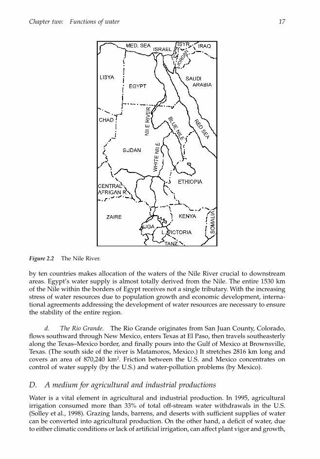
c. The Nile River.
The conflict on the water allocation of the Nile River is moresevere than those in the two Middle East regions described above. The White Nile origi-nates in the highlands of Rwanda and Burundi, flows into the huge basin of Lake Victoriain Tanzania, then travels northward through Kenya, Uganda, Congo, Central AfricanRepublic, Ethiopia, Sudan, and Egypt, and then empties into the Mediterranean Sea. AtKhartoum, Sudan, the Blue Nile, originating from Lake Tana in Ethiopia, merges with theWhite Nile to form a total drainage area of 3,050,000 km
2
. The river sprawls from aboutlat. 5
∞
S to lat. 31.5
∞
N and covers about one tenth of the African continent (Figure 2.2).Although the Nile (6825 km) is the longest river in the world, its annual discharge is
only a small proportion of that of other major rivers, for example, 3% of the Amazon, 14%of the Mississippi, and 43% of the Danube (Said, 1981). The low volume of waters shared
1363_C02_fm Page 16 Tuesday, December 3, 2002 6:59 AM
Chapter two: Functions of water 17
by ten countries makes allocation of the waters of the Nile River crucial to downstreamareas. Egypt’s water supply is almost totally derived from the Nile. The entire 1530 kmof the Nile within the borders of Egypt receives not a single tributary. With the increasingstress of water resources due to population growth and economic development, interna-tional agreements addressing the development of water resources are necessary to ensurethe stability of the entire region.
d. The Rio Grande.
The Rio Grande originates from San Juan County, Colorado,flows southward through New Mexico, enters Texas at El Paso, then travels southeasterlyalong the Texas–Mexico border, and finally pours into the Gulf of Mexico at Brownsville,Texas. (The south side of the river is Matamoros, Mexico.) It stretches 2816 km long andcovers an area of 870,240 km
2
. Friction between the U.S. and Mexico concentrates oncontrol of water supply (by the U.S.) and water-pollution problems (by Mexico).
D. A medium for agricultural and industrial productions
Water is a vital element in agricultural and industrial production. In 1995, agriculturalirrigation consumed more than 33% of total off-stream water withdrawals in the U.S.(Solley et al., 1998). Grazing lands, barrens, and deserts with sufficient supplies of watercan be converted into agricultural production. On the other hand, a deficit of water, dueto either climatic conditions or lack of artificial irrigation, can affect plant vigor and growth,
Figure 2.2
The Nile River.
1363_C02_fm Page 17 Tuesday, December 3, 2002 6:59 AM
18 Forest Hydrology: An Introduction to Water and Forests
the quantity and quality of production, seedling survival, litter production, and fertilizeruptake. Worldwide, about 18% of cropland is irrigated, making crop production two tothree times greater than that from rain-watered land (Miller, 1999).
Although irrigation is beneficial to agricultural production, inappropriate water man-agement can create salinization and waterlogging problems on irrigated land. Irrigationwater contains salts. Evapotranspiration of irrigation water leaves salts behind in the soil,and the salts accumulate to a harmful level through prolonged irrigation practices. Salin-ization retards crop growth and yields, and eventually ruins the land. Farmers oftenreclaim saline soils by applying a large amount of irrigation water to leach salts throughthe soil profile. However, inadequate underground drainage makes water accumulateunder the ground. The water table then gradually rises to the root zone and soaks andeventually kills the plants.
Water is used for the cooling processes in steam electric-generation plants and ascoolant, solvent, lubricant, cleansing agent, conveying agent, screening agent, and reagentin most industrial manufacturing processes. For example, it takes about 55 to 390 t ofwater to fabricate 1 t of paper, and 9 to190 t of water to make 1 t of textiles. Total industrialuse of water accounted for more than 54% of all withdrawals and consumptive uses ofwater in the U.S. in 1995.
1. HydroponicsWater, by making a nutrient solution containing all the essential elements required byplants for normal growth and development, can be used to culture vegetables, fruits, andflowers in a variety of environments. The technique is referred to as water culture, or moreprofessionally as hydroponics, meaning “water working.” Today, hydroponics is inclu-sively referred to as the science of growing plants by media other than soils, such as water,gravel, sand, peat, sawdust, vermiculite, or pumice.
The growing of plants in water dates back to several hundred years B.C. in Babylon,China, Greece, and Egypt, but modern techniques were not developed until the plants’macro- and micronutrients were discovered in the late 1880s and early 1890s. DuringWorld War II, the U.S. military applied hydroponics to grow fresh vegetables and foodfor troops stationed on nonarable islands in the Pacific (Resh, 1989). Today, the entirehydroponic system, due to the development of plastics, vinyl, suitable pumps, time clocks,plastic plumbing, solenoid valves, and other equipment, can be automatically operatedat costs a fraction of those in the past. Large commercial installations exist throughout theworld.
Hydroponics is particularly valuable in countries with little land or limited arableland and large populations. City dwellers and hotel managers may find it attractive togrow plants in living rooms, along hallways, and on porches or windowsills for decoration.Many citizens in Taipei, Taiwan, grow vegetables as supplemental crops on their rooftops.The technique can be used in atomic submarines, spaceships, or space stations.
The crop yield per unit area by hydroponics is about 4 to 30 times higher than soilculture under field conditions (Resh, 1989). This may be due to several reasons, includinghigh planting density, more efficient use of water and fertilizers, less environmentaldamage, and low operational costs. Soil culture requires regular control of weeds, andmay have problems with soilborne diseases, insects, and animal attacks. It needs croprotation to overcome build-up of infestation and nutrient-deficiency problems. Hydropon-ics does not encounter these problems.
In traditional soil culture, plants must develop large root systems to absorb elementsrequired for development and growth. However, the availability of nutrients in the soildepends upon soil bacteria to break down organic matter into elements and soil water todissolve elements into solutions. With hydroponics, nutrients are immediately available
1363_C02_fm Page 18 Tuesday, December 3, 2002 6:59 AM

Chapter two: Functions of water 19
to plants. It takes only 1/20 to 1/30 the amount of water required by conventional soilgardening.
All these advantages lead hydroponics to be the quickest and simplest method forproducing the maximum amount of vegetables from a minimum area (DeKorne, 1992).
2. Fish cultureFish culture or farming, in which fish and shellfish are raised for food, began in Chinaaround 2000 B.C. (Lee, 1981). As of 1993, about 15.7 million metric tons or 15.5% of thetotal global fish harvest were raised artificially through fish farming, 10.1% from inlandfarming, and 5.4% from marine farming (FAO, 1995a). It supplies 60% of the fish con-sumption in Israel, 40% in China, and 22% in Indonesia (Miller, 1999).
Fish farming usually involves stocking fish in ponds or containers until they reachthe desired size (inland farming) or holding captured species in fenced-in areas or floatingcages in lagoons or estuaries until maturity (marine farming). Surveys conducted by FAOshow 1028 species that have been farmed around the world and summarize them into sixcategories (World Resources Institute et al., 1996):
Freshwater fish: e.g., carp, barbel, and tilapiaDiadromous fish: e.g., sturgeon, river eel, salmon, trout, and smeltMarine fish: e.g., flounders, cod, redfish, herring, tuna, mackerel, and sharksCrustaceans: e.g., crabs, lobsters, shrimps, and prawnsMolluscs: e.g., oysters, mussels, scallops, clams, and squidOthers: includes frogs, turtles, and aquatic plants
FAO (1995b) projects that global fish farming will need to double by 2010 in order tomeet the steady increase in demand. Overfishing has been a serious problem in worldfisheries since the early 1980s. It has caused 25% of the stock to be seriously depleted andput another 44% at their biological limit (World Resources Institute et al., 1996). A reduc-tion of 30 to 50% fishing intensity has been suggested to return the oceans to healthy andsustainable fisheries. The reduction, if carried out, will cause the supply of seafood tocome from fish farming.
Although fish farming produces high yields per unit area, the rapid growth of fishfarming is subject to some environmental risks. Without proper pollution-control mea-sures, the wastes generated from fish farms can contaminate surface streams, lakes,groundwater, and bay estuaries. Some of the ecologically important mangrove forests inEcuador, the Philippines, Panama, Indonesia, Honduras, and other less-developed coun-tries have been destroyed by fish farming (Miller, 1999; FAO, 1995b).
3. A tool for industrial operationsThrough extreme pressure and speed, water can even be used as a tool to remove the barkof trees (hydraulic debarker) and cut rocks or other materials. In construction, water jetswith high speed and pressure are used to excavate mountains and cut tunnels in massiveconstruction projects. Using hydraulic principles, hydraulic jacks and levels can raise orlower heavy loads precisely with a small force.
The Bureau of Mines designed a water-jet perforator, which issues a high-velocitywater jet, to penetrate nonmetallic well casings for the purpose of completing or stimu-lating in situ uranium-leaching wells (Savanick and Krawza, 1981). In situ uranium leach-ing is a mining method in which wells are drilled from the surface to the mineralizedrock. An oxidizing leaching solution is injected through these wells into the uraniferousrock. The solution dissolves the uranium minerals, and the uraniferous solution is subse-
1363_C02_fm Page 19 Tuesday, December 3, 2002 6:59 AM
20 Forest Hydrology: An Introduction to Water and Forests
quently drawn into another well. It is then pumped to a processing plant where theuranium is extracted and precipitated as uranium oxide.
Uraniferous ore is usually formed in consolidated sandstones. Thus, a well screen atthe base of the casing adjacent to the ore is necessary to assure fluid flow between thewellbore and the ore and to prevent caving of the ore and sand. The water-jet device,having a flow of at least 7 gpm at 10,000 psi, is lowered into the wellbore and penetratesthe well casing, cement, and the surrounding uraniferous sandstone. The perforationallows leaching solution to pass between the sandstone and the wellbore, enhances localpermeability of the mineralized zone, and saves time and energy.
ReferencesBerry, G.W., Grim, P.J., and Ikelman, J.A., 1980, Thermal Springs List for the U.S., U.S. National
Oceanic and Atmospheric Administration, National Geophy. and Solar-Terrestrial Data Cen-ter, Boulder, CO.
Bloom, A.L., 1978, Geomorphology — A Systematic Analysis of Late Cenezoic Landforms, Prentice Hall,New York.
Changnon, S.A., Jr. and Jones, D.M.A., 1972, Review of the influences of the Great Lakes on weather,Water Resour. Res., 8, 360–371.
Clarke, R., 1993, Water: The International Crisis, MIT Press, Cambridge, MA.Dahl, T.E., 1990, Wetlands Losses in the U.S. 1780s to 1980s, U.S. Fish and Wildlife Service, Wash-
ington, D.C.Dahl, T.E. and C.E. Johnson, 1991, Wetlands Status and Trends in the Conterminous U.S., mid-
1970s–1980s, U.S. Fish and Wildlife Service, Washington D.C.DeKorne, J.B., 1992, The Hydroponic Hot House, Loompanics Unlimited, Port Townsend, WA.der Leeden, F.V., Troise, F.L., and Todd, D.K., 1990, The Water Encyclopedia, Lewis Publishers, Chelsea,
MI.FAO, 1995a, Global Fish and Shellfish Production in 1993, Food and Agriculture Organization of
the United Nations, FAO Fisheries Dept., Fisheries Information, Data and Stat. Service, Rome.FAO, 1995b, Review of the State of World Fishery Resources: Aquaculture, FAO Fisheries Circular
No. 886, Food and Agriculture Organization of the United Nations, Rome.Floyd, C., 1990, America’s Great Disasters, Mallard Press, New York.Fowler, G., 1991, Crazy Water, Texas Christian University Press, Fort Worth, TX.Hillel, D., 1994, Rivers of Eden, the Struggle for Water and the Quest for Peace in the Middle East, Oxford
University Press, Oxford.Lee, J., 1981, Commercial Catfish Farming, Interstate Printer & Publishers, Inc., Danville, IL.Leopold, L.B. and K.S. Davis, 1972, Water, Silver Burdett Co., Morristown, NJ.Miller, G.T., Jr., 1999, Environmental Science: Working with the Earth, 7th ed., Wadsworth, Belmont, CA.Muryn, M., 1995, Water Magic, Simon & Schuter, New York.Resh, H.M., 1989, Hydroponics Food Production, Woodbridge Press, Sant Barbara, CA.Richardson, C.J., 1994, Ecological functions and human values in wetlands: a framework for assess-
ing forestry impacts, Wetlands, 14, 1–9.Said, R., 1981, The Geological Evolution of the River Nile, Springer-Verlag, Heidelberg.Savanick, G.A. and Krawza, W.G., 1981, Water Jet Perforation, A New Method for Completing and
Stimulating In Situ Leaching Wells, Rep. of Investigations 8569, U.S. Dept. of the Interior.Solley, W.B., Pierce, R.R., and Perlman, H.A., 1998, Estimated Use of Water in the U.S. in 1995, U.S.
Geological Survey Circular 1200, Washington, D.C.Ting, J.C., 1989, Conflict Analysis of Allocating Freshwater Inflows to Bays and Estuaries — A Case
Study on Choke Canyon Dam and Reservoir, Texas, Doctoral Dissertation, College of Forestry,Stephen F. Austin State University, Nacogdoches, TX.
UNESCO, 1992, Water and Health. IHP Humid Tropics Programme Series No.3. Division of WaterSciences, Paris.
1363_C02_fm Page 20 Tuesday, December 3, 2002 6:59 AM

Chapter two: Functions of water 21
U.S. National Weather Service, 1975, Climatological Data Annual Summary, California, Nebraska,and Iowa, National Climatic Data Center, Asheville, NC.
U.S. U.S. News & World Report, 1983, War over water, crisis of the ’80s, U.S. News & World Report,October 31, 1983,. 57–62.
U.S. Water News, 1996a, Water fuel is on track, U.S. Water News, 12, 1, 4.U.S. Water News, 1996b, Israel refuses to give up a drop of water from Golan Heights, U.S. Water
News, 12, 2.World Resources Institute, the United Nations, and the World Bank, 1996, World Resources, a Guide
to the Global Environment, 1996–97, Oxford University Press, Oxford.
1363_C02_fm Page 21 Tuesday, December 3, 2002 6:59 AM

1363_C02_fm Page 22 Tuesday, December 3, 2002 6:59 AM
23
chapter three
Water as a science
Contents
I. Water in history .................................................................................................................23A. Asia..............................................................................................................................23B. Middle East ................................................................................................................25C. Europe.........................................................................................................................26D. The United States......................................................................................................27
II. Hydrosciences ....................................................................................................................28A. Hydrology ..................................................................................................................28
1. Disciplines in hydrology ...................................................................................28a. On the body of waters .................................................................................29b. On land-surface conditions .........................................................................30c. On interdisciplinary studies........................................................................32
References .......................................................................................................................................34
Early humans experienced water with reverence, superstition, folklore, fear, and specula-tion on the one hand, and on the other hand showed many ingenious ways of utilizingwater. Water has been a topic for systematic measurement and scientific study since the17th century. We shall first provide an overview of significant events in water managementand development, and then introduce the disciplines of water science.
I. Water in history
The history of water-resources management is an integral part of the history of civilization(Bennett, 1939; Frank, 1955). The floodplains along China’s Yellow River, Egypt’s NileRiver, India’s Ganges, and Babylon’s Tigris and Euphrates cradled the four oldest civili-zations of the world. Yet, history has taught us how the depletion of soil and waterresources caused by wars among nations and tribes have caused the fall of cities, countries,and even civilizations. An ancient Chinese proverb, “To rule the mountains is to rule thewaters,” reveals the general principle learned from these incidents — that upstreamwatershed management is necessary for control of downstream flooding.
A. Asia
Early civilizations worked strenuously and continuously to reduce flooding at higherlatitudes, where precipitation is greater than evaporation, and to develop and conserve
1363_C03_fm Page 23 Wednesday, December 4, 2002 7:38 AM
24 Forest Hydrology: An Introduction to Water and Forests
water resources at the lower latitudes, where evaporation exceeds precipitation. In China,Emperor Yau (about 2880 B.C.) put a man, Yu, in charge of flood control in North China.Because of the success of Yu’s dams, dikes, diversion ditches and other works on theYellow River, he was chosen to succeed Emperor Shun as the ruler of China, and is knownas “Yu, the Great.”
From old documents and recent archeological evidence, we know that the ancientChinese had the skills for digging wells for drinking water as early as six or seven thousandyears ago (Young, 1985). A well excavated at Ho-Moo-Du, Yee-Yau in the Tse-KiangProvince of China is believed to have been built during the New Stone Ages. The wellwas cased by four rows of logs with a squared frame attached to the logs at the top ofthe well. Also excavated were more than 60 tile wells southwest of Peking that are believedto have been built around 600 B.C. for drinking and irrigation. Figure 3.1 is a mechanicalwater wheel used in Tang Dynasty (618–907 A.D.) for agricultural irrigation and domesticwater supply.
In central China, the Tukianguien irrigation system, built by Lee Bien about 2200 yearsago, was an ingenious multipurpose water-resources project (Wang, 1983). The projectdiverted the flow of the Ming River, a tumultuous stream emerging from the Tibetanplateau, through a series of dams and dikes on the main river where it first enters thebroad plain from a mountain canyon. It employed bamboo frames weighted down byrocks to dam or divert the water, a spillway to adjust flow volume in the river, and periodicdredging activity when sediment built to a certain level, as indicated by stone marks inthe channel. The project irrigated about 200,000 ha of fertile soils, reducing greatly theheavy toll of life and property resulting from spring and summer floods. As a result, theMing River basin became the most productive region of China. In turn, the river providedthe necessary resources to enable Chin Shihuang (the “First Chin Emperor”) to overthrowthe Chow Dynasty and its feudal lords, making China a unified country. Even today, thesystem is still the major agricultural water supply in the region.
Another great water project in Asia is the Grand Canal of China, the longest waterwaysystem of the world. The canal integrates the peoples and economies of the North, South,
Figure 3.1
An ancient hydraulic wheel and a pedal irrigator in the Tang Dynasty (618–907 A.D.).
1363_C03_fm Page 24 Wednesday, December 4, 2002 7:38 AM

Chapter three: Water as a science 25
inland, and coastal areas into a single political–economic entity. It was the economic arteryand a political arm over six major dynasties, from the Sui to the Ching. It had two majorperiods of development. The first period began in 584 A.D. during the Sui Dynasty,connecting and expanding upon preexisting waterways to form a two-branch water sys-tem. One branch extended northeasterly from the Yellow River at Luoyang, the easterncapital in central China, to today’s Beijing, about 800 km in length. The other branchextended southeasterly from Luoyang through the Huai River basin to the Yangtze Riverregion, also about 800 km. The second period of development started in 1283 A.D. duringthe Yuan Dyansty, stretching the canal between the capital city Beijing in the north toHangzhou in the south with a total length of about 1100 km (Chen et al., 1992). Variationsin climate, geology, topography, and elevation between north and south are great, and afew major rivers cross all the regions. The development and construction of the canalsystem reflects the ingenuity and technological skill of the Chinese.
Lo Lan was a small country located on the western bank of Lop Nor (a salt lake nowdried), Sinkiang between 300 B.C. and 400 A.D. It was a trading center in the middle ofthe silk routes between China and countries in the Near East during the Han Dynasty.The area was covered with beautiful forests, fertile soils, and thick pastures nourished byflowing rivers and springs. However, the country disappeared after 400 A.D., and the areais dry and barren today, leaving a series of questions. Recent archaeological work revealedthat Lo Lan had a full set of laws regarding taxes, water conservancy, lands, hunting,forest protection, criminals, and property. The forest-protection law set the fine for erad-icating a living tree at one horse and for chopping tree’s limbs at one head of cattle. Theimportance of forests for the control of soil erosion, sand-dune stabilization, and protectionof stream siltation was well recognized. It was probably the earliest law regarding forestsand environment in the world (Southern Chinese Daily News, 1997).
B. Middle East
In drier and lower latitudes, the people of Assyria, Babylon, Egypt, and Israel beganconstruction of water supply and drainage systems about 5000 years ago. Egyptians hadcore drilling in rock for wells as early as 3000 B.C. The world’s oldest known dam wasbuilt by the Egyptians in about 3000 B.C. to store drinking and irrigation water. Perhapsit also controlled flooding waters. The dam was a rock-fill structure, about 108 m longand with a crest of about 12 m above the riverbed. It failed soon after construction.However, a Roman reservoir in Jordan (Jacob’s well) was so well-built that it holds watertoday (Frank, 1955). Small earth and masonry dams built by the Roman Empire were usednot only to store runoff water but also to raise the general water level in streams (TheUnited Nations Environmental Program, 1983).
The oldest streamflow records in the world are recognized as the markings of theflood stages of the Nile River carved in its cliffs between Semneh and Kumneh around2000 B.C. (Boyer, 1964), and mention of annual flooding of the Nile dates back to between3000 and 3500 B.C. In the lower reach of the Nile River, annual floods deposit rich sedimentalong the floodplains, which makes the land agriculturally productive. Thus, the cropyields in the Nile valley are dependent upon the annual flood of the river, and the floodstage in the Nile each year was a criterion for taxation in early Egypt. The Egyptianpharaoh Menes developed a flood-control system for the Nile River more than 3000 yearsago that included at least 20 recording stations (Grant, 1992). These stations used a crudestaff gage — referred to today as the Nilometer—to measure the water level, s, probablythe oldest hydrometric in the world.
In and around the third millennium B.C., well-planned city drainage and water-supplysystems, public toilets, and baths were constructed with burnt bricks along the Indus River
1363_C03_fm Page 25 Wednesday, December 4, 2002 7:38 AM
26 Forest Hydrology: An Introduction to Water and Forests
in Pakistan. Most houses in the capital city Mohenjo Daro, discovered in the early 20thcentury, were supplied with water from household wells as deep as 25 m. The averagedistance between wells was about 35 m in an area of at least 300 ha. Artificial elevationwas constructed on the residential areas to survive the threat of the river’s annual inun-dation (Jansen, 1999).
Records on central water supply and wastewater disposal date back about 5000 yearsto Nippur of Sumeria. The Sanskrit medical lore of India and Egyptian wall inscriptionstaught that foul water can be purified by boiling, exposure to sunlight, filtering throughcharcoal, and cooling in a tile vessel. These teachings were verified by the English philos-opher Sir Francis Bacon, who in 1627 published experiments on the purification of waterby filtration, boiling, distillation, and clarification by coagulation. Bacon stated that puri-fying water tends to improve health and increase the pleasure of the eye (Viessman andHammer, 1985).
C. Europe
Early Europe made many important contributions to water utilization and management.The collection of water by rain harvesting dates back to prehistorical times in Europe.Designs have been found in the ruins of the palace of Knossos (1700 B.C.), the center ofMinoan Crete. Small courts were built between the western and eastern wings of thepalace. Besides providing light for the lower floors, these courts collected rainwater, whichwas drained out for ritual activities and air conditioning. Rainwater also was collectedfrom the roof, channeled to small cisterns, and stored for various purposes (The UnitedNations Environmental Program, 1983).
Waterwheels for irrigation, water supply, and milling corn were used in ancient Greeceand Rome. However, due to the scarcity of cheap slave and animal labor, the applicationof waterpower did not become widespread until the 12th century.
Concerns about water and environment were documented in the 13th century. LouisVI of France promulgated “The Decree of Waters and Forests” in 1215, considered to bethe earliest written document in the West concerning the relation between waters andforests (Kittredge, 1948). However, analysis of such a relationship was not addressed untilthe 1830s, when systematic streamflow measurements became available. Dr. HeinrichBerghaus, a German hydrographer, found that the streamflows in the Elbe and Oder riversgradually decreased from 1778 to 1835. He attributed the decrease of streamflows to thedestruction of forests, cultivation of the soil, and the draining of swamps. In 1873, anAustrian hydrographer, Gustave Wex, attributed the diminishment of water in the Rhine,Elbe, Oder, Vistula, and Danube rivers to the decrease in precipitation which, in turn, wasdue to forest destruction (Zon, 1927). Wex’s works generated a great interest in the relationbetween waters and forests in Europe in the 19th century and were well accepted by manyprominent scientists, although his interpretations are no longer acceptable in the light ofmodern hydrology.
In 1837, a special commission set up to investigate the causes of decreasing riverdischarge in Russia concluded that it was due to deforestation and expanding agriculturalacreage. Later, G. Wex also blamed the severe droughts occurring through most of Europein 1870 to the effects of expanding agriculture (Molchanov, 1963). In 1860, France begana reforestation program in a region where some 320,000 ha of farmland had been seriouslydamaged as a result of clearcutting on the headwaters of streams. The planting programresulted in complete control of damage from 163 torrents, 31 of which were consideredhopeless about a half-century earlier. It was then concluded that forest cover is one of themost effective means of erosion control and that the best place to control streamflow is atthe headwaters of streams.
1363_C03_fm Page 26 Wednesday, December 4, 2002 7:38 AM
Chapter three: Water as a science 27
A German scientist, Krutsch, started the first investigation of the effects of forest uponprecipitation under a pine stand in 1863. Over a period of 16 months, he found thatthroughfall was merely 9% when rainfall was very light (not over 0.5 mm), and it mightamount to 80 to 90% in case of strong showers (Molchanov, 1963; Friedrich, 1967).
There was also a great interest in the forest and floods relationship in the last part ofthe 19th century in Europe. The first scientific watershed research on the effects of forestupon streamflow regularity was initiated by the Swiss Central Experimental Station in1890 (Zon, 1927). Two small watersheds of similar topography, geological formation, soil,and latitude, but different in forest cover (one was 98% forested while the other was 30%)were selected for the study. Rainfall, snowfall, runoff, and temperature data for these twowatersheds were collected carefully using recording or nonrecording gages. The prelimi-nary result based on 11 years of data showed: (1) the deforested watershed carried 30 to50% more water per unit of area during the high flood periods; (2) the lowflows werehigher in the forested watershed; and (3) total annual discharges of the two watershedswere about the same. The streamflow discharge in the forested watershed was moreuniform than that of the deforested watershed.
D. The United States
America inherited many of the European concepts about water and forests. Many conser-vationists claimed that deforestation caused floods in wet seasons and made streams andcreeks drier in the summer. Conversely, the existence of forest could prevent floods becausetree-root systems held soil in place, and soil stored moisture. Thus, streamflow benefitedin the dry seasons from the slow release of stored water and by the increase of precipitationin the forested area.
The forest-streamflow hypothesis and consequent conservation movement inevitablygenerated disputes, conflicts, and controversies in the U.S. (Walker, 1983; Pisani, 1992).The disputes extended from the 19th century to the early 20th century. Hiram M. Chit-tenden, an officer in the U.S. Army Corps of Engineers, presented a paper titled “Forestsand Reservoirs in Their Relation to Streamflow with Particular Reference to NavigableStreams” at the 1908 annual meeting of the American Society of Civil Engineers. He statedthat forests did not prevent floods, the main benefit of forests being to protect soil fromerosion. Willis L. Moore, chief of the Weather Bureau, issued a pamphlet in 1910 entitled“A Report on the Influence of Forests on Climate and on Floods,” which aimed to showthat forests were an insignificant factor in floods. This opposition was forcefully attackedby the chief of the U.S. Forest Service, Gifford Pinchot, who stated in 1910, “The connectionbetween forests and rivers is like that between father and son. No forests, no rivers” (Sartz,1983). The heated debate and nationwide campaign of the Forest Service led to the passageof the Weeks Act in 1911 (Douglas and Hoover, 1987). The act authorized federal purchasesof forestlands in the headwaters of navigable streams and federal matching funds forapproved state agencies to protect forested watersheds of navigable streams.
Although there was no agreement with respect to the relationship between forestsand floods, many realized that the deficiencies in scientific information and experimentaldata for justification needed to be addressed. The first experimental watershed project ofthe U.S., similar to that of the Swiss study, was established in 1910 at Wagon Wheel Gap,headwaters of the Rio Grande in Colorado, and continued until 1926. The project, a jointeffort between the Forest Service and the Weather Bureau, was designated to comparestreamflows from a denuded watershed and an undisturbed, forested watershed. Similarwatershed experiments included the San Gabriel River basin in Southern California (1917),San Dimas, California (1935), White Hollow Watersheds, Tennessee (1934), Coweeta, NorthCarolina (1933), Fraser Experimental Forest, Colorado (1937), H. J. Andrews Watersheds,
1363_C03_fm Page 27 Wednesday, December 4, 2002 7:38 AM
28 Forest Hydrology: An Introduction to Water and Forests
Oregon (1948), Hubbard Brook, New Hampshire (1955), Parsons, West Virginia (1955),Oxford, Mississippi (1957), and many others. Today, at least 440 major experimentalwatersheds are located at 49 different areas throughout the United States (Figure 12.1).
The concerns of the U.S. Congress about stream-water quality were manifested by thepassage of the Rivers and Harbors Act in 1899. The act prohibited discharge of refuse intowaterways or deposits of materials on the bank of any navigable waters. It was the firstlegislation to include nonpoint sources of water pollution in a federal program. However,it was not until the end of World War II that the concerns became more widespread anda series of laws passed to regulate national water-quality conditions caused by variousland uses and industrial activities. Major water-pollution acts include: the Federal WaterPollution Control Act of 1948 (PL80–845) and Amendments of 1956 (PL84–660) and of1961 (PL87–88), Water Quality Act of 1965 (PL89–234), Clear Water Restoration Act of 1966(PL89–753), Water Quality Improvement Act of 1970 (PL91–224), Federal Water PollutionControl Act Amendments of 1972 (PL92–500), Clear Water Act of 1977 (PL95–217), andWater Quality Act of 1987.
II. Hydrosciences
A. Hydrology
The scientific study of water, called hydrology, is a branch of earth science. It is concernedwith the problems of water on the earth. Such problems may involve water quantity andquality, interrelations between water and environment, and the impact of man’s activityon the occurrence, circulation, and distribution of water. Hydrology looks for the causesand effects of these problems, predicts water-related events and problems, and studiesthe adjustment, management, and operation of water and water resources to benefit societyand the environment.
Man’s interest in water may be as old as our civilization. The source of water in streamsand springs was a puzzling problem that was the subject of much speculation and con-troversy until a comparatively recent time. King Solomon, who lived nearly 1000 yearsbefore Christ, wrote in the Old Testament that all streams flow into the sea but the sea isnever full. The Greek philosophers, such as Thales (about 650 B.C.), Plato (427–347 B.C.)and Aristotle (about 384–322 B.C.), developed ideas that the springs and streams aresupplied from the ocean, driven into rocks by winds, and elevated in the mountains, byrock pressure, by vacuum produced by the flows of springs, by pressure exerted on thesea, or by the virtue of the heavens.
The French physicist Pierre Perrault (1608–80) quantitatively demonstrated that rain-fall in the Seine River is sufficient to account for discharge by the river. Soon after Perrault,the English astronomer Edmund Halley (1656–1742) made observations on the rate ofevaporation. He demonstrated that evaporation from the Mediterranean Sea was ampleto supply the quantity of water returned to that sea by rivers (Meinzer, 1942). Thesescientists unveiled our modern concept of the hydrologic cycle and initiated quantitativestudies of modern hydrology.
1. Disciplines in hydrology
Water can be found in solid, liquid, and gaseous states at common earth temperatures.The presence of water, changes in water from one state to another, and water translocationand storage serve environmental, biological, and sociological functions. Hydrologyembraces such a large and diversified field that no one can study it all. The broad scienceof hydrology, more properly called hydroscience, is further broken down into disciplines
1363_C03_fm Page 28 Wednesday, December 4, 2002 7:38 AM
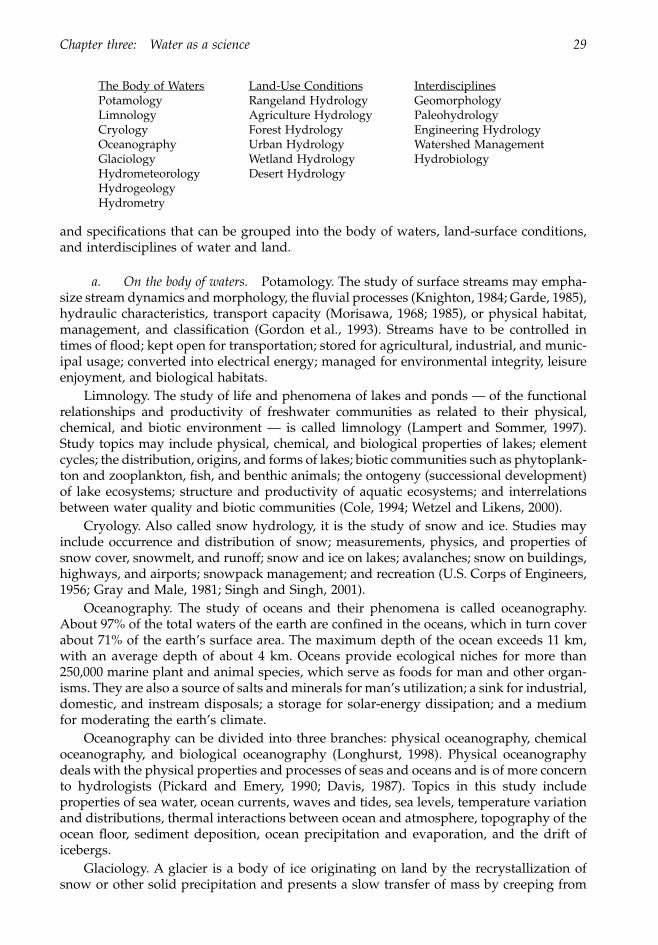
Chapter three: Water as a science 29
and specifications that can be grouped into the body of waters, land-surface conditions,and interdisciplines of water and land.
a. On the body of waters.
Potamology. The study of surface streams may empha-size stream dynamics and morphology, the fluvial processes (Knighton, 1984; Garde, 1985),hydraulic characteristics, transport capacity (Morisawa, 1968; 1985), or physical habitat,management, and classification (Gordon et al., 1993). Streams have to be controlled intimes of flood; kept open for transportation; stored for agricultural, industrial, and munic-ipal usage; converted into electrical energy; managed for environmental integrity, leisureenjoyment, and biological habitats.
Limnology. The study of life and phenomena of lakes and ponds — of the functionalrelationships and productivity of freshwater communities as related to their physical,chemical, and biotic environment — is called limnology (Lampert and Sommer, 1997).Study topics may include physical, chemical, and biological properties of lakes; elementcycles; the distribution, origins, and forms of lakes; biotic communities such as phytoplank-ton and zooplankton, fish, and benthic animals; the ontogeny (successional development)of lake ecosystems; structure and productivity of aquatic ecosystems; and interrelationsbetween water quality and biotic communities (Cole, 1994; Wetzel and Likens, 2000).
Cryology. Also called snow hydrology, it is the study of snow and ice. Studies mayinclude occurrence and distribution of snow; measurements, physics, and properties ofsnow cover, snowmelt, and runoff; snow and ice on lakes; avalanches; snow on buildings,highways, and airports; snowpack management; and recreation (U.S. Corps of Engineers,1956; Gray and Male, 1981; Singh and Singh, 2001).
Oceanography. The study of oceans and their phenomena is called oceanography.About 97% of the total waters of the earth are confined in the oceans, which in turn coverabout 71% of the earth’s surface area. The maximum depth of the ocean exceeds 11 km,with an average depth of about 4 km. Oceans provide ecological niches for more than250,000 marine plant and animal species, which serve as foods for man and other organ-isms. They are also a source of salts and minerals for man’s utilization; a sink for industrial,domestic, and instream disposals; a storage for solar-energy dissipation; and a mediumfor moderating the earth’s climate.
Oceanography can be divided into three branches: physical oceanography, chemicaloceanography, and biological oceanography (Longhurst, 1998). Physical oceanographydeals with the physical properties and processes of seas and oceans and is of more concernto hydrologists (Pickard and Emery, 1990; Davis, 1987). Topics in this study includeproperties of sea water, ocean currents, waves and tides, sea levels, temperature variationand distributions, thermal interactions between ocean and atmosphere, topography of theocean floor, sediment deposition, ocean precipitation and evaporation, and the drift oficebergs.
Glaciology. A glacier is a body of ice originating on land by the recrystallization ofsnow or other solid precipitation and presents a slow transfer of mass by creeping from
The Body of Waters Land-Use Conditions InterdisciplinesPotamology Rangeland Hydrology GeomorphologyLimnology Agriculture Hydrology PaleohydrologyCryology Forest Hydrology Engineering HydrologyOceanography Urban Hydrology Watershed ManagementGlaciology Wetland Hydrology HydrobiologyHydrometeorology Desert HydrologyHydrogeologyHydrometry
1363_C03_fm Page 29 Wednesday, December 4, 2002 7:38 AM
30 Forest Hydrology: An Introduction to Water and Forests
region to region. The study of ice and glaciers in all aspects is termed glaciology. Thescope may include formation of ice in the ground, glacier classification, runoff, movement,climatic effects and changes, and hydrologic problems related to glaciers (Meier, 1966;Hutter, 1983; The Geological Society of America, 1999; Singh and Singh, 2001).
Hydrometeorology. Meteorology deals with the movement of water in the atmosphere,while hydrology is concerned with the distribution and occurrence of water on and underthe earth’s surface. The hydrologic cycle is a concern common to both sciences. Thus, theapplication of meteorology to hydrological problems such as developing water resourcesand flood control is called hydrometeorology (or hyetology, precipitation hydrology).Major topics may include the estimation of probable maximum precipitation, storm mod-els, temporal and spatial variations of storms, storm transposition, engineering designand river forecasting, and accuracy and representativeness of precipitation measurements.(Bruce and Clark, 1966; Wiesner, 1970; Am. Water Resour. Assoc., 1983; Upadhyay, 1996).
Hydrogeology. More than 22% of all freshwaters on Earth are confined under theground, while surface water in lakes and rivers makes up only about 0.36%. Currently,about 80% of water withdrawals in the United States come from streams and lakes.Groundwater is then logically seen as a major resource for easing water-shortage problems.In fact, groundwater is even more desirable than surface water due to: (1) no pathogenicorganisms in general, (2) constancy of temperature and chemical composition, (3) absenceof turbidity and color, (4) no effects of short droughts on supplies, and (5) difficulty ofradiochemical and biological contamination. However, groundwater development maybe difficult in some areas due to its costs, low permeability, land subsidence problems,and great content in dissolved solids. The science that studies groundwater occurrence,distribution, and movement is called hydrogeology or groundwater hydrology (Davis andDeWiest, 1966; Palmer and Peterson, 1991). The exploration of groundwater, the effects ofgeological environment on groundwater chemistry and mode of migration, and ground-water contamination are also interesting subjects to many hydrogeologists.
Hydrometry. The science of water measurements is called hydrometry. More than 3000years ago the Egyptian pharaoh Menes developed the first staff gage, now called theNilometer, to monitor the water level of the Nile River (Leupold & Stevens, Inc., 1987).The Nilometer was marked in graduations on walls to obtain a visual reading of the waterlevel on-site (Kolupaila, 1960). Today water is measured in terms of water level, velocity,discharge, and depth, and it can be measured manually, semiautomatically, and automat-ically with radio and satellite communication systems and computer data storage andmanipulation capability (Ackers et al., 1978; WMO, 1980; USGS, 1985; Herschy, 1999;Boiten, 2000).
b. On land-surface conditions.
Rangeland Hydrology. Land on Earth may be clas-sified into five categories: nonproductive land (about 15%), forestland (30%), rangeland(40%), cropland (10%), and urban-industrial land (5%). Rangelands are natural grasslands,savannas, shrublands, most deserts, tundra, alpine communities, coastal marshes, and wetmeadows. Rangelands are often are intermingled with other types of land and are dis-tributed from sea level to above timberline. These lands are more suitable for managementby ecological principles than for management by economic principles. Rangeland vege-tation is predominantly short, consisting of broad-leafed plants such as grasses, forbs, andshrubs. It provides a variety of natural resources including forage, livestock, fish andwildlife, minerals, recreation, and water beneficial to man in both tangible and intangibleaspects. The study of hydrologic principles as applied to rangeland ecosystems is calledrangeland hydrology. Topics associated with rangeland hydrology may include vegetationmanagement in relation to water loss and conservation; grazing impact on surface runoff,
1363_C03_fm Page 30 Wednesday, December 4, 2002 7:38 AM
Chapter three: Water as a science 31
soil erosion, stream sedimentation, and water quality; snowpack management, and waterharvesting (Branson et al., 1981; American Soc. of Agri. Engineers, 1988).
Agricultural Hydrology. Water use for agricultural irrigation and raising livestock isthe greatest single use in the U.S., accounting for 41.8% of the total water utilized in 1985,while thermoelectric, industrial, and domestic uses of water were 38.7%, 9.1%, and 10.4%,respectively (Paulson et al., 1988). The study of application of hydrologic principles toagricultural development, production, and management is called agrohydrology. Landdrainage, irrigation, water harvesting, water conservation, soil erosion and sedimentation,water quantity, and quality of surface and groundwater are some major topics and con-cerns in agricultural hydrology (van Hoorn, 1988).
Forest Hydrology. With respect to its height, density, and thickness of crown canopy,fluffy forest floor, spread root system, and wide horizontal distribution and vertical cov-erage, forest is the most distinguished type of vegetation on the earth. Generally, forestsprosper in regions where the minimum net radiation is 20,000 1 y yr
-
1
and the minimumprecipitation is 500 mm yr
-
1
. Those areas are the major sources of our surface water fordomestic and industrial use. In the U.S., for example, forests occupy about 30% of thetotal territory, yet this 30% of land area produces about 60% of total surface runoff.Harvesting and other activities in the forest area will inevitably disturb forest canopiesand floors, consequently affecting the quantity, quality, and timing of water resources. Thegeographical significance of forestland, along with the uniqueness of forest ecosystems,makes the study of water in forested areas a specification of scientific study.
The study of water in forest areas was largely covered under the discipline of forestinfluences in the first half of this century. All effects of natural vegetation on climate, water,and soil are under the scope of forest influences. By the middle of the century, Kittredge(1948) suggested that the water phases of forest influences be called forest hydrology.
Forest hydrology is a study of hydrology in forestland. It is concerned with forest,and forest activity in relation to all phases of water — an interdisciplinary science thatbrings forest and hydrology together. Thus, all the influences of forest cover along withforest management and activity on precipitation, streamflow, evapotranspiration, soilwater, floods, drought, soil erosion, stream sediment, nutrient losses, and water qualityare within the scope of forest hydrology. It provides the basic knowledge, principles,scientific evidence, and justification for managing water resources in forested watersheds.Topics in forest hydrology are discussed in detail by Penman (1963), Monke (1971), Lee(1980), and Black (1991).
Studies extending issues in forest–water relations to plant–water relations may becalled “eco-hydrology” (Baird and Wilby, 1999) or “environmental hydrology” (Ward andElliot, 1995).
Urban Hydrology. The physical environment of urban and industrial areas is com-pletely different from that of forests, agricultural lands, and rangeland. Many observationsand studies have shown greater precipitation in and around major urban areas than inthe surrounding countryside due to the enormous number of condensation nuclei pro-duced by human activities and atmospheric instability associated with the heat islandgenerated by the city (Sayok and Chang, 1991). The impervious surfaces created by urbandevelopment may cause an increase in flooding, soil erosion, stream sedimentation, andpollution of land and water bodies (American Public Works Asso., 1981; Lazaro, 1990).The study of hydrology in urban areas and the hydrologic problems associated withurbanization fall within the scope of urban hydrology.
Wetland Hydrology. Wetlands are areas where the water table is at or near the surfaceof the land for at least a consecutive period of time, or is covered by shallow water up to2 m (6 ft) deep. The abundant water in the soils makes soil properties significantly differentfrom those in the uplands and the soil is suitable for growth of certain plant species. Five
1363_C03_fm Page 31 Wednesday, December 4, 2002 7:38 AM
32 Forest Hydrology: An Introduction to Water and Forests
major wetland systems have been recognized: marine, estuaries, lacustrine, riverine, andpalustrine. Marine and estuaries systems are coastal wetlands, such as tidal marshes andmangrove swamps. Lacustrine and riverine wetlands are associated with lakes and rivers,respectively. The last system includes marshes, swamps, and bogs (Niering, 1987). Thus,wetlands are transitional zones between aquatic and terrestrial ecosystems, all rich inplants and animals.
Water is the primary factor that controls the environment, plants, animals, and soils.Wetlands are no longer wastelands as they were thought to be in the past. They are notonly habitats of a variety of plant and animal species, but also important natural flood-control mechanisms, nature’s water-purification plants, nutrient and food suppliers toaquatic organisms, a major contributor to groundwater recharge, and a buffer zone forshoreline erosion (Chang, 1987). Wetland hydrology studies vegetation and flooding,hydrologic characteristics of wetlands, streamflow, and sediment. It examines the impactof development projects on wetland ecosystems, groundwater fluctuation, water quality,nutrient removal and transformation, wetland construction and restoration, wetland man-agement, soil characteristics, wetlands delineation and classification, erosion control, etc.(Marble, 1992; Lyon, 1993; U.S. Environmental Protection Agency, 1993; Gilman, 1994).
Desert Hydrology. Although arid and semiarid lands cover about 30% of the world’sland area, only about 15% of the world’s population lives in these regions. However, theregions are of strategic and economic importance because these regions contain over one-half of the precious and semiprecious minerals and most of the oil and natural gas. Hererainfall is little, highly variable, and infrequent. Coupling rainfall scarcity with great ratesof soil and water evaporation makes water deficiency a general phenomena and charac-teristic across the region. A vast area depends on springs and groundwater for its watersupply. Desert hydrology studies the characteristics and processes of the hydrology cyclein arid and semiarid areas, springs, and groundwater resources. It also examines waterconservation and harvesting, the adaptation of plants to the environment, hydro-climatechanges, decertification, and water quality (Beaumont, 1993; Shahin, 1996).
c. On interdisciplinary studies.
Geomorphology. Geomorphology is concernedwith landforms and drainage characteristics created by running water and other physicalprocesses. The study of drainage basins and channel networks was largely qualitative anddeductive prior to the 1950s. Dr. Arthur N. Strahler and his Columbia University associateshave made great contributions to transform the science from descriptive into quantitativestudy. Geomorphology provides an invaluable basis for assessing the potential of land fordevelopment, for land-use planning, and for environmental management (Cooke andDoornkamp, 1990). Since the behavior of streamflow is highly affected by watershedtopographic characteristics (Wolman et al., 1995), the quantitative description of drainagebasins and channel networks enables hydrologists to evaluate the spatial variations ofstreamflow, precipitation, temperature, snow distribution, and other hydro-climatic vari-ables, and consequently to produce hydrologic models and simulations (Verstappen, 1983;Wilson and Gallant, 2000).
Paleohydrology. Many hydraulic structures are designed to meet climatic and hydro-logic conditions 50 to 100 years in the future. The estimation of these future events isbased on data collected in the past. Accuracy of these estimates is affected greatly by dataavailability and representativeness of the data observations. If a short period of hydrologicdata recorded in a relatively dry period were used in the analysis, the designed flood fora structure might well be too small to accommodate large floods in wet periods. Thephysical and financial success of such a project might be seriously jeopardized. Paleohy-drology is the study of hydrologic conditions in ancient times. The study may be usefulin understanding the changes in precipitation, temperature, stream levels, and water
1363_C03_fm Page 32 Wednesday, December 4, 2002 7:38 AM
Chapter three: Water as a science 33
balance from the past to modern times, defining the physical laws that govern the fluc-tuations of hydrologic conditions, and studying environmental change on continents(Gregory et al., 1996; Benito et al., 1998). It is related to paleoclimatology (Cronin, 1999).Techniques used in the study may include tree rings (dendrochronology), glacial fluctu-ations, fossils, pollen deposition in bogs (palynology), sediment cores in deep seas andlakes, and other geological evidence.
Engineering Hydrology. Hydrological information is essential in the design, operation,and management of flood-control works, irrigation systems, water-supply projects, storm-runoff drainage, erosion controls, highway culverts, and many other hydraulic structures.Engineering hydrology is the study of hydrologic characteristics of a watershed or adrainage system required to solve these engineering problems. The study may includefrequency analysis of hydrologic events, depth–area–duration analysis, estimation ofevapotranspiration, hydrograph analysis, streamflow routing, rain–runoff relations,streamflow simulation, estimation of soil erosion and stream sedimentation, risk analysis,and many others (Linsley et al., 1975).
Watershed Management. Due to gravitation, rainwater is always drained from placesof higher elevation to a lower elevation. All land enclosed by a continuous hydrologicdrainage divide and lying up-slope from a specific section on a stream is a watershed.Thus, every piece of land belongs to one watershed or another, depending on the referencesection in question, and in any watershed all surface water is drained out through thatparticular section in the channel. The watershed, also called a catchment or drainage basin,is the unit of land area that the hydrologist and watershed manager consider for studyor management. It is analogous to the silviculturist’s stand, or the forest manager’s com-partment. However, stand and compartment may be a more or less artificial unit, whilewatersheds have natural boundaries.
Watersheds have been employed as social and economic units for community devel-opment and conservation of natural resources including water, soils, forests, wildlife, andothers. Because of the steadily increasing demands for water in our modern society andthe fact that much of the water for agriculture, industry, recreation, and domestic use hasits source in forested land, watershed management has become increasingly important toforesters. Thus, watershed management is management of all natural resources includingforests, land, wildlife, recreation, and minerals within a watershed for the protection andproduction of water resources while maintaining environmental stability.
Accordingly, watershed management is water oriented; it is primarily concerned withwater resources and related problems. Since soil erosion may greatly affect water quality,flood damage, land deterioration, environmental aesthetics, and many other factors, thesoil stabilization and prevention of soil erosion is also one of the most important chal-lenges in protecting water resources, an area that is generally covered under the disciplineof soil conservation. Soil conservation is soil oriented, and ignorance of water movementcauses severe soil erosion and environmental problems. Thus watershed managementand soil conservation share the same concerns in some areas. In reality, watershed man-agement involves much more complex problems and broader tasks than soil conservation.It deals with water as well as soil problems, along with land planning and resourcemanagement activities in upstream forested land, while soil conservation deals with soilproblems relating to land productivity in downstream agricultural regions. In a sense,watershed management is integrated resources management for the production andprotection of watershed water resources and should properly be called “integrated water-shed management.”
Watershed management is based on principles in forest hydrology and the knowledgein general hydrology, meteorology, climatology, ecology, soils and geology, engineering,land planning, environmental regulation, and social science. It is essential that the atmo-
1363_C03_fm Page 33 Wednesday, December 4, 2002 7:38 AM
34 Forest Hydrology: An Introduction to Water and Forests
spheric, plant, soil, and water systems of the watershed — and frequently the impact ofman’s activity on the complex system — be considered simultaneously. Ignorance of anyone variable may make watershed projects costly and ineffective. Detailed discussions ofwatershed management are given by Colman (1953), FAO (1977), Hamilton and King(1983), Brooks et al. (1991), and Satterlund and Adams (1992).
Hydrobiology. Aquatic plants can be grouped into six categories based upon size,shape, and growth habits: plankton algae, filamentous algae, submersed weeds, emergedweeds, marginal weeds, and floating weeds. Extensive infestations of these plants createproblems in water for recreation, irrigation, flood control, and navigation, increase waterloss due to transpiration, and organism-transmitted diseases, and affect physical proper-ties. Topics such as the characteristics of aquatic plants, plant distribution, plant growthand development, aquatic plants and environment, and control and management of theseplants are interesting to hydrobiologists (Gangstad, 1986; Riemer, 1993; Caffrey, 2000).
Other disciplines such as medical hydrology (water in relation to human health), andhydroecology (water and its environmental and physiological functions) also have beenmentioned in the literature.
References
Ackers, P. et al., 1978,
Weirs and Flumes for Flow Measurement
, John Wiley & Sons, New York.American Public Works Association, 1981,
Urban Stormwater Management
, APWA Research Founda-tion, Chicago.
American Soc. of Agri. Engineers, 1988, Modeling Agricultural, Forest, and Rangeland Hydrology,
Proceedings of the 1988 International Symposium
, St. Joseph, MI.American Water Resour. Assoc., 1983, International Symposium on Hydrometeorology, Bethesda,
MD.Baird, A.J. and Wilby, R.L., 1999,
Eco-Hydrology
, Routledge, New York.Beaumont, P., 1993,
Drylands: Environmental Management and Development
, Routledge, New York.Benito, G., Baker, V.R., and Gregory, K.J., Eds., 1998,
Paleohydrology and Environmental Change
, JohnWiley & Sons, New York.
Bennett, H.H., 1939,
Soil Conservation
, McGraw-Hill, New York.Black, P.E., 1991,
Watershed Hydrology
, Prentice Hall, New York.Boiten, W., 2000,
Hydrometry
, Balkema Publishers, Rotterdam.Boyer, M.C., 1964, Streamflow measurement, in
Handbook of Applied Hydrology
, Chow, V.T., Ed.,McGraw-Hill, New York.
Branson, F.A. et al., 1981,
Rangeland Hydrology
, Kendall/Hunt, Dubuque, IA.Brooks, K.N. et al., 1991,
Hydrology and the Management of Watersheds
, Iowa State University Press,Ames, IA.
Bruce, J.P. and Clark R.H., 1966,
Introduction to Hydrometeorology
, Pergamon Press, Elmsford, NY.Caffrey, J.M., Ed., 2000,
Biology, Ecology and Management of Aquatic Plants
, Kluwer, Dordrecht.Chang, M., 1987, Monitoring bottomland hardwoods in response to hydrologic changes below dams,
in
Bottomland Hardwoods in Texas
, McMahan, C.A. and Frye, R.G., Eds., Texas Parks andWildlife Department, pp. 162–164.
Chen, M.T. et al., 1992,
Brief Histories of the Chinese Sciences and Technology
, Ming-Wen Book Co., Taipei.Cole, G.A., 1994, T
extbook of Limnology
, Waveland Press, Prospect Heights, IL.Colman, E.A., 1953, V
egetation and Watershed Management
, Ronald Press, New York.Cooke, R.U. and Doornkamp, J.C., 1990,
Geomorphology in Environmental Management: A New Intro-duction
, Clarendon Press, Oxford.Cronin, T.M., 1999,
Principles of Paleoclimatology
, Columbia University Press, Irvington, NY.Davis, R.A., 1987,
Oceanography: An Introduction to Marine Environment
, W.C. Brown, Dubugne, IA. Davis, S.N. and DeWiest, R.J.M., 1966,
Hydrogeology
, John Wiley & Sons, New York.Douglas, J. E. and Hoover, M.J., 1987, History of Coweeta, in
Forest Hydrology and Ecology at Coweeta
,Swank, W.T. and Crossley, D.A., Jr., Eds., Springer-Verlag, Heidelberg.
1363_C03_fm Page 34 Wednesday, December 4, 2002 7:38 AM

Chapter three: Water as a science 35
FAO, 1977, Guidelines for Watershed Management, Food and Agri. Organ. of the United Nations,Rome.
Frank, B., 1955, The story of water as the story of man, in Water, the Yearbook of Agr., USDA,Washington, D.C.
Friedrich, W., 1967, Forest hydrology research in Germany, in
International Symposium on ForestHydrology
, Sopper, W.E. and Lull, H.W., Eds., Pergamon Press, Elmsford, NY.Gangstad, E.O., 1986,
Freshwater Vegetation Management
, Thomas Publications, Fresno, CA.Garde, R.J., 1985,
Mechanics of Sediment Transportation and Alluvial Stream Problems
, John Wiley &Sons, New York.
Gilman, 1994, Geological Society of America, 1999,
Glacial Processes, Past and Present
, Boulder, CO.Gordon, N.D., McMahon, T.A., and Finlayson, B.L., 1993, Stream Hydrology. John Wiley & Sons,
New York.Grant, D.M., 1992,
ISCO Open Channel Flow Measurement Handbook
, 3rd ed., ISCO, Inc., Lincoln, NE.Gray, D.M., and Male, D.H., 1981,
Handbook of Snow
, Pergamon Press, Elmsford, NY.Gregory, K.J., Starkel, L., and Baker, V.R., Eds., 1996,
Global Continental Paleohydrology
, John Wiley &Sons, New York.
Hamilton, L.S. and King, P.N., 1983,
Tropical Forested Watersheds, Hydrologic and Soils Response to MajorUses or Conversions
, Westview Press, Boulder.Herschy, R.W., Ed., 1999, Hydrometry: Principles and Practices, 2nd ed., John Wiley & Sons, New
York.Hutter, K., 1983,
Theoretical Glaciology: Material Science of Ice and the Mechanics of Glaciers and Ice Sheets
,Reidel/Terra, Dordrecht.
Jansen, M.R.N., 1999, Mohenjo Daro and the River Indus, in
The Indus River — Biodiversity, Resources,and Humankind
, Meadows, A. and Meadows, P.S., Eds., Oxford University Press, Oxford.Kittredge, J., 1948,
Forest Influences
, McGraw-Hill, New York.Knighton, D., 1984,
Fluvial Forms and Processes
, Edward Arnold, London.Kolupaila, S., 1960, Early history of hydrometry in the United States,
Proc. Am. Soc. Civil Eng.,J. Hydrau. Div
., 86, 1–50.Lampert, W. and Sommer, U., 1997,
Limnoecology: The Ecology of Lakes and Streams
, Oxford UniversityPress, Oxford.
Lazaro, T.R., 1990,
Urban Hydrology — A Multidisciplinary Perspective, Technomic
, Lancaster, PA.Lee, R., 1980,
Forest Hydrology
, Columbia University Press, New York.Leupold & Stevens, Inc., 1987, Stevens Water Resources Data Book, Beaverton, OR.Linsley, R.K., Jr., Kohler, M.A., and Paulhus J.L.H., 1975,
Hydrology for Engineers
, 2nd ed., McGrawHill, New York.
Longhurst, A.R., 1998,
Ecological Geography of the Sea
, Academic Press, New York.Lyon, J. G., 1993,
Practical Handbook for Wetland Identification and Delineation
, Lewis Publishers, BocaRaton, FL.
Marble, A.D., 1992,
A Guide to Wetland Functional Design
, Lewis Publishers, Boca Raton, FL.Meier, M.F., 1966, Ice and glaciers, in
Handbook of Applied Hydrology
, Chow, V.T., Ed., McGraw-Hill,New York, pp. 16:1–32.
Meinzer, O.E., 1942,
Hydrology
, Dover, New York.Molchanov, A.A., 1963, The Hydrological Role of Forests, Israel Program for Scientific Translations,
U.S. Dept. of Agriculture.Monke, E.J., Ed., 1971, Biological Effects in the Hydrological Cycle,
Proc. of the Third InternationalSeminar for Hydrology Professors
, Dept. of Agr. Eng., Purdue Univ., West Lafayette, IN.Morisawa, M., 1968,
Streams, Their Dynamics and Morphology
, McGraw-Hill, New York.Morisawa, M., 1985,
Rivers
, Longman, New York.Niering, W.A., 1987,
Wetlands
, Alfred A. Knopf, New York.Palmer, C.M. and Peterson, J.L., 1991,
Principles of Contaminant Hydrogeology
, Lewis Publishers, BocaRaton, FL.
Paulson, R.W., Chase, E.B., and Carr, J.E., 1988, Water supply and use in the United States: U.S.Geological Survey National Water Summary 1987, in Water-Use Data for Water ResourcesManagement, Waterstone, M. and Burt, R.J., Eds., Amer. Water Resour. Assoc., TPS-88–2,Bethesda, MD.
1363_C03_fm Page 35 Wednesday, December 4, 2002 7:38 AM
36 Forest Hydrology: An Introduction to Water and Forests
Penman, H.L., 1963,
Vegetation and Hydrology
, Commonwealth Agr. Bureaux, Farnham Royal, Buks,England.
Pickard, G.L. and Emery, W.J., 1990,
Descriptive Physical Oceanography: An Introduction
, 5th ed.,Pergamon Press, Elmsford, NY.
Pisani, D.J., 1992,
To Reclaim a Divided West: Water, Law, and Public Policy, 1848–1902
, University ofNew Mexico Press, Albuquerque.
Riemer, D.N., 1993,
Introduction to Freshwater Vegetation
, Krieger Publ. Co., Melbourne, FL.Sartz, R.S., 1983, Watershed management, in
Encyclopedia of American Forest and Conservation History
,Vol. ll, Davis, R.C., Ed., MacMillan, New York.
Satterlund, D.R. and Adams, P.W., 1992,
Wildland Watershed Management
, John Wiley & Sons, NewYork.
Sayok, A.K. and Chang, M., 1991, Rainfall in and around the city of Nacogdoches, Texas,
Texas J. Sci
.,43, 173–178.
Shahin, M., 1996,
Hydrology and Scarcity of Water Resources in Arab Region
, A.A. Balkema, Rotterdam.Singh, P. and Singh, V., 2001,
Snow and Glacier Hydrology
, Klumer Academic Publishers, Hingham,MA.
Southern Chinese Daily News, 1997, Exploring the Secrecy of Lop Nor: Archaeologists revealed thelife styles of Lo Lanian (Editoral),
Southern Chinese Daily News
, December 28, 1997.United Nations Environmental Program, 1983,
Rain and Sormwater Harvesting in Rural Areas
, TycoolyInternational Publ. Ltd., Dublin, Ireland.
Upadhyay, D.S., 1996,
Cold Climate Hydrometeorology
, John Wiley & Sons, New York.U.S. Corps of Engineers, 1956, Snow Hydrology, North Pacific Div., Portland, OR.U.S. Environmental Protection Agency, 1993, Created and Natural Wetlands for Controlling Non-
point Source Pollution, Office of Wetlands, Oceans, and Watersheds, Washington, D.C.USGS, 1985, Techniques of Water-Resources Investigations of the United States Geological Survey,
Alexandria, VA.van Hoorn, J.W., 1988, Agrohydrology — recent developments,
Proc. Symp. Agrohydrology
, Wagenin-gen, The Netherlands, 29 Sept. – 1 Oct. 1987, Elsevier, New York.
Verstappen, H.T., 1983,
Applied Geomorphology
, Elsevie, New York.Viessman, W., Jr. and Hammer, M.J., 1985,
Water Supply and Pollution Control
, Harper & Row, NewYork.
Walker, L.C., 1983, Forest influences, in
Encyclopedia of American Forest and Conservation History
, Vol.I, Davis, R.C., Ed., Macmillan and Free Press, New York.
Wang, P., 1983, A brief history of engineering technology in China, in
The History of Science andTechnology in China
, Vol. ll, Wu, L.C., Ed., Natural Sci. and Culture Publ. Co., Taipei, pp.255–262.
Ward, A.D. and Elliot, W.J., Eds., 1995,
Environmental Hydrology
, Lewis Publishers, Boca Raton, FL.Wetzel, R.G. and Likens, G.E., 2000,
Limnological Analyses
, Springer-Verlag, Heidelberg.Wiesner, C.J., 1970,
Hydrometeorology
, Chapman & Hall, London.Wilson, J.P. and Gallant, J.C., Eds., 2000,
Terrain Analysis: Principles and Applications
, John Wiley &Sons, New York.
WMO, 1980,
Manual on Stream Gauging
, Operational Hydrology Report No. 13, WMO-NO. 519,World Meteorological Organization,.
Wolman, M.G., Miller, J.P., and Leopold, LB., 1995,
Fluvial Processes in Geomorphology
, Dover Pub-lishers, Mineola, NY.
Young, L.S., 1985, How did our ancestors utilize groundwater?
International Daily News
, March 2 (inChinese).
Zon, R., 1927,
Forests and Water in the Light of Scientific Investigation
, U.S. Forest Service, Washington,D.C.
1363_C03_fm Page 36 Wednesday, December 4, 2002 7:38 AM

37
chapter four
Properties of water
Contents
I. Physical properties............................................................................................................38A. Three states of water ................................................................................................38B. Latent heat of water .................................................................................................38C. Saturation vapor pressure .......................................................................................39D. Vapor diffusion..........................................................................................................39E. Heat capacity .............................................................................................................40F. Thermal conductivity ...............................................................................................41
II. Hydraulic properties ........................................................................................................41A. Density........................................................................................................................42B. Pressure ......................................................................................................................42C. Buoyancy....................................................................................................................44D. Surface tension and capillary rise..........................................................................45E. Viscosity......................................................................................................................46F. The Reynolds number..............................................................................................46G. Shear stress.................................................................................................................47H. Stream power ............................................................................................................48
III. Chemical properties..........................................................................................................48A. The water molecule ..................................................................................................48B. Formation of water...................................................................................................49C. Chemical reactions....................................................................................................49
IV. Biological properties .........................................................................................................50A. Temperature ...............................................................................................................50B. Dissolved oxygen......................................................................................................51C. pH................................................................................................................................52D. Conductivity ..............................................................................................................53E. Sediment.....................................................................................................................54
References .......................................................................................................................................55
Water is the most vital and ubiquitous substance on Earth. It has been described as amiracle of nature, the mirror of science, and the blood of life. Many properties of waterare used as references and standards for properties of other substances. This chapterexamines water properties from four perspectives: physical, hydraulic, chemical, andbiological.
1363_C04_fm Page 37 Wednesday, December 4, 2002 7:39 AM
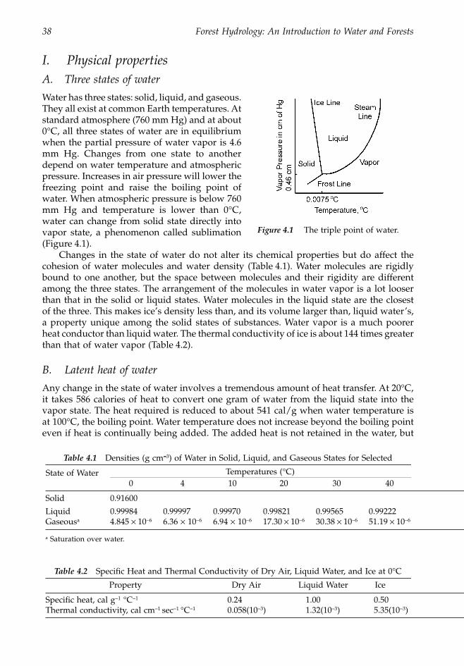
38 Forest Hydrology: An Introduction to Water and Forests
I. Physical properties
A. Three states of water
Water has three states: solid, liquid, and gaseous.They all exist at common Earth temperatures. Atstandard atmosphere (760 mm Hg) and at about0
∞
C, all three states of water are in equilibriumwhen the partial pressure of water vapor is 4.6mm Hg. Changes from one state to anotherdepend on water temperature and atmosphericpressure. Increases in air pressure will lower thefreezing point and raise the boiling point ofwater. When atmospheric pressure is below 760mm Hg and temperature is lower than 0
∞
C,water can change from solid state directly intovapor state, a phenomenon called sublimation(Figure 4.1).
Changes in the state of water do not alter its chemical properties but do affect thecohesion of water molecules and water density (Table 4.1). Water molecules are rigidlybound to one another, but the space between molecules and their rigidity are differentamong the three states. The arrangement of the molecules in water vapor is a lot looserthan that in the solid or liquid states. Water molecules in the liquid state are the closestof the three. This makes ice’s density less than, and its volume larger than, liquid water’s,a property unique among the solid states of substances. Water vapor is a much poorerheat conductor than liquid water. The thermal conductivity of ice is about 144 times greaterthan that of water vapor (Table 4.2).
B. Latent heat of water
Any change in the state of water involves a tremendous amount of heat transfer. At 20
∞
C,it takes 586 calories of heat to convert one gram of water from the liquid state into thevapor state. The heat required is reduced to about 541 cal/g when water temperature isat 100
∞
C, the boiling point. Water temperature does not increase beyond the boiling pointeven if heat is continually being added. The added heat is not retained in the water, but
Table 4.1
Densities (g cm
----
3
) of Water in Solid, Liquid, and Gaseous States for Selected
State of Water
Temperatures (°C)0 4 10 20 30 40
Solid 0.91600
Liquid 0.99984 0.99997 0.99970 0.99821 0.99565 0.99222Gaseous
a
4.845
¥
10
-
6
6.36
¥
10
-
6
6.94
¥
10
-
6
17.30
¥
10
-
6
30.38
¥
10
-
6
51.19
¥
10
-
6
a
Saturation over water.
Table 4.2
Specific Heat and Thermal Conductivity of Dry Air, Liquid Water, and Ice at 0°C
Property Dry Air Liquid Water Ice
Specific heat, cal g
-
1
°C
-
1
0.24 1.00 0.50Thermal conductivity, cal cm
-
1
sec
-
1
∞
C
-
1
0.058(10
-
3
) 1.32(10
-
3
) 5.35(10
-
3
)
Figure 4.1 The triple point of water.
1363_C04_fm Page 38 Wednesday, December 4, 2002 7:39 AM
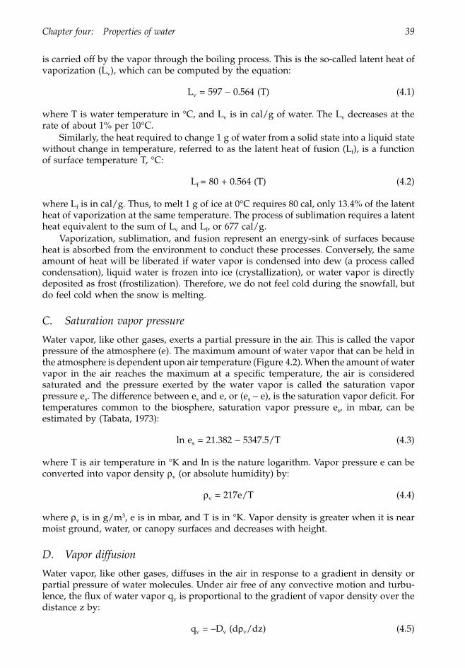
Chapter four: Properties of water 39
is carried off by the vapor through the boiling process. This is the so-called latent heat ofvaporization (L
v
), which can be computed by the equation:
L
v
= 597
-
0.564 (T) (4.1)
where T is water temperature in
∞
C, and L
v
is in cal/g of water. The L
v
decreases at therate of about 1% per 10
∞
C.Similarly, the heat required to change 1 g of water from a solid state into a liquid state
without change in temperature, referred to as the latent heat of fusion (L
f
), is a functionof surface temperature T,
∞
C:
L
f
= 80 + 0.564 (T) (4.2)
where L
f
is in cal/g. Thus, to melt 1 g of ice at 0
∞
C requires 80 cal, only 13.4% of the latentheat of vaporization at the same temperature. The process of sublimation requires a latentheat equivalent to the sum of L
v
and L
f
, or 677 cal/g.Vaporization, sublimation, and fusion represent an energy-sink of surfaces because
heat is absorbed from the environment to conduct these processes. Conversely, the sameamount of heat will be liberated if water vapor is condensed into dew (a process calledcondensation), liquid water is frozen into ice (crystallization), or water vapor is directlydeposited as frost (frostilization). Therefore, we do not feel cold during the snowfall, butdo feel cold when the snow is melting.
C. Saturation vapor pressure
Water vapor, like other gases, exerts a partial pressure in the air. This is called the vaporpressure of the atmosphere (e). The maximum amount of water vapor that can be held inthe atmosphere is dependent upon air temperature (Figure 4.2). When the amount of watervapor in the air reaches the maximum at a specific temperature, the air is consideredsaturated and the pressure exerted by the water vapor is called the saturation vaporpressure e
s
. The difference between e
s
and e, or (e
s
-
e), is the saturation vapor deficit. Fortemperatures common to the biosphere, saturation vapor pressure e
s
, in mbar, can beestimated by (Tabata, 1973):
ln e
s
= 21.382
-
5347.5/T (4.3)
where T is air temperature in
∞
K and ln is the nature logarithm. Vapor pressure e can beconverted into vapor density
r
v
(or absolute humidity) by:
r
v
= 217e/T (4.4)
where
r
v
is in g/m
3
, e is in mbar, and T is in °K. Vapor density is greater when it is nearmoist ground, water, or canopy surfaces and decreases with height.
D. Vapor diffusion
Water vapor, like other gases, diffuses in the air in response to a gradient in density orpartial pressure of water molecules. Under air free of any convective motion and turbu-lence, the flux of water vapor q
v
is proportional to the gradient of vapor density over thedistance z by:
q
v
= –D
v
(d
r
v
/dz) (4.5)
1363_C04_fm Page 39 Wednesday, December 4, 2002 7:39 AM
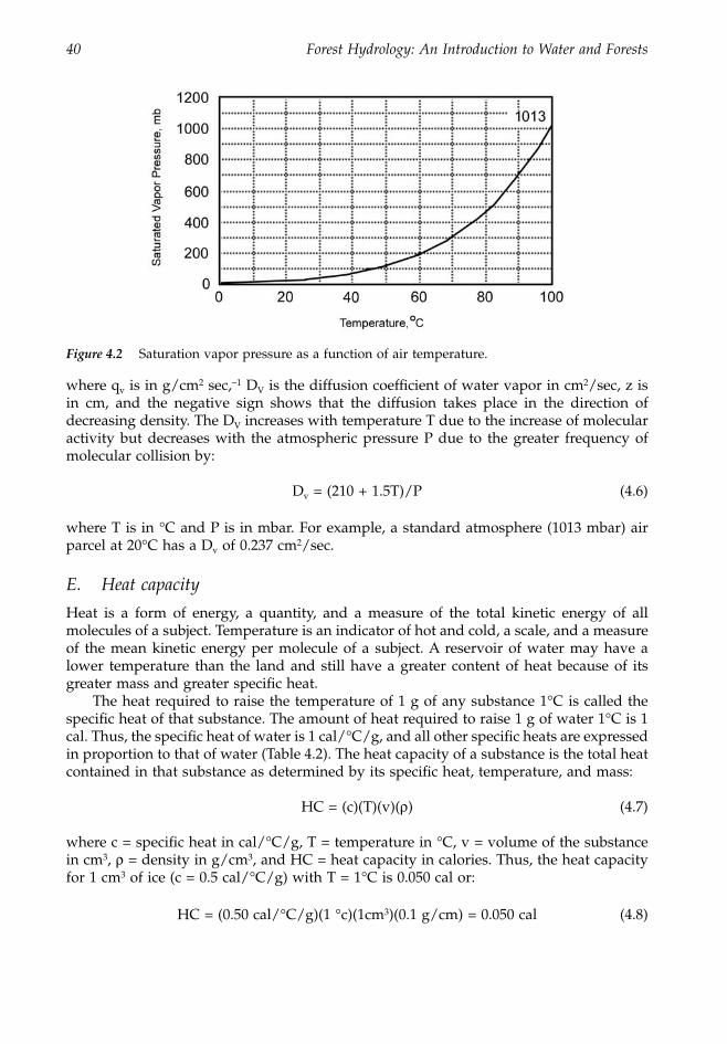
40 Forest Hydrology: An Introduction to Water and Forests
where q
v
is in g/cm
2
sec,
-
1
D
V
is the diffusion coefficient of water vapor in cm
2
/sec, z isin cm, and the negative sign shows that the diffusion takes place in the direction ofdecreasing density. The D
V
increases with temperature T due to the increase of molecularactivity but decreases with the atmospheric pressure P due to the greater frequency ofmolecular collision by:
D
v
= (210 + 1.5T)/P (4.6)
where T is in
∞
C and P is in mbar. For example, a standard atmosphere (1013 mbar) airparcel at 20
∞
C has a D
v
of 0.237 cm
2
/sec.
E. Heat capacity
Heat is a form of energy, a quantity, and a measure of the total kinetic energy of allmolecules of a subject. Temperature is an indicator of hot and cold, a scale, and a measureof the mean kinetic energy per molecule of a subject. A reservoir of water may have alower temperature than the land and still have a greater content of heat because of itsgreater mass and greater specific heat.
The heat required to raise the temperature of 1 g of any substance 1
∞
C is called thespecific heat of that substance. The amount of heat required to raise 1 g of water 1
∞
C is 1cal. Thus, the specific heat of water is 1 cal/
∞
C/g, and all other specific heats are expressedin proportion to that of water (Table 4.2). The heat capacity of a substance is the total heatcontained in that substance as determined by its specific heat, temperature, and mass:
HC = (c)(T)(v)(
r
) (4.7)
where c = specific heat in cal/
∞
C/g, T = temperature in
∞
C, v = volume of the substancein cm
3
,
r
= density in g/cm
3
, and HC = heat capacity in calories. Thus, the heat capacityfor 1 cm
3
of ice (c = 0.5 cal/
∞
C/g) with T = 1
∞
C is 0.050 cal or:
HC = (0.50 cal/
∞
C/g)(1
∞
c)(1cm
3
)(0.1 g/cm) = 0.050 cal (4.8)
Figure 4.2
Saturation vapor pressure as a function of air temperature.
1363_C04_fm Page 40 Wednesday, December 4, 2002 7:39 AM
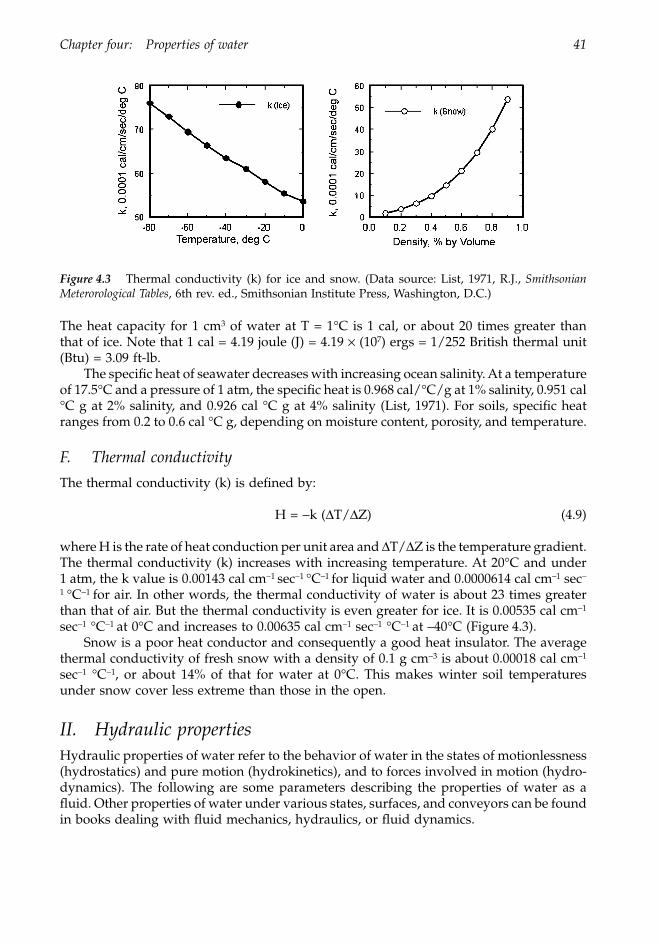
Chapter four: Properties of water 41
The heat capacity for 1 cm
3
of water at T = 1
∞
C is 1 cal, or about 20 times greater thanthat of ice. Note that 1 cal = 4.19 joule (J) = 4.19
¥
(10
7
) ergs = 1/252 British thermal unit(Btu) = 3.09 ft-lb.
The specific heat of seawater decreases with increasing ocean salinity. At a temperatureof 17.5
∞
C and a pressure of 1 atm, the specific heat is 0.968 cal/
∞
C/g at 1% salinity, 0.951 cal
∞
C g at 2% salinity, and 0.926 cal
∞
C g at 4% salinity (List, 1971). For soils, specific heatranges from 0.2 to 0.6 cal
∞
C g, depending on moisture content, porosity, and temperature.
F. Thermal conductivity
The thermal conductivity (k) is defined by:
H =
-
k (
D
T/
D
Z) (4.9)
where H is the rate of heat conduction per unit area and
D
T/
D
Z is the temperature gradient.The thermal conductivity (k) increases with increasing temperature. At 20
∞
C and under1 atm, the k value is 0.00143 cal cm
-
1
sec
-
1
∞
C
–1
for liquid water and 0.0000614 cal cm
–1
sec
-
1
∞
C
-
1
for air. In other words, the thermal conductivity of water is about 23 times greaterthan that of air. But the thermal conductivity is even greater for ice. It is 0.00535 cal cm
-
1
sec
-
1
∞C-1 at 0∞C and increases to 0.00635 cal cm-1 sec-1 ∞C-1 at –40∞C (Figure 4.3).Snow is a poor heat conductor and consequently a good heat insulator. The average
thermal conductivity of fresh snow with a density of 0.1 g cm-3 is about 0.00018 cal cm–1
sec-1 ∞C-1, or about 14% of that for water at 0∞C. This makes winter soil temperaturesunder snow cover less extreme than those in the open.
II. Hydraulic propertiesHydraulic properties of water refer to the behavior of water in the states of motionlessness(hydrostatics) and pure motion (hydrokinetics), and to forces involved in motion (hydro-dynamics). The following are some parameters describing the properties of water as afluid. Other properties of water under various states, surfaces, and conveyors can be foundin books dealing with fluid mechanics, hydraulics, or fluid dynamics.
Figure 4.3 Thermal conductivity (k) for ice and snow. (Data source: List, 1971, R.J., SmithsonianMeterorological Tables, 6th rev. ed., Smithsonian Institute Press, Washington, D.C.)
1363_C04_fm Page 41 Wednesday, December 4, 2002 7:39 AM
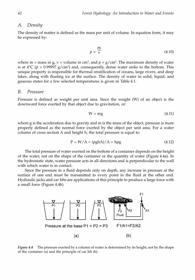
42 Forest Hydrology: An Introduction to Water and Forests
A. Density
The density of matter is defined as the mass per unit of volume. In equation form, it maybe expressed by:
r = (4.10)
where m = mass in g, v = volume in cm3, and r = g/cm3. The maximum density of wateris at 4∞C (r = 0.99997 g/cm3) and, consequently, dense water sinks to the bottom. Thisunique property is responsible for thermal stratification of oceans, large rivers, and deeplakes, along with floating ice at the surface. The density of water in solid, liquid, andgaseous states for a few selected temperatures is given in Table 4.1.
B. Pressure
Pressure is defined as weight per unit area. Since the weight (W) of an object is thedownward force exerted by that object due to gravitation, or:
W = mg (4.11)
where g is the acceleration due to gravity and m is the mass of the object, pressure is moreproperly defined as the normal force exerted by the object per unit area. For a watercolumn of cross section A and height h, the total pressure is equal to:
P = W/A = (rghA)/A = hrg (4.12)
The total pressure of water exerted on the bottom of a container depends on the heightof the water, not on the shape of the container or the quantity of water (Figure 4.4a). Inthe hydrostatic state, water pressure acts in all directions and is perpendicular to the wallwith which water is in contact.
Since the pressure in a fluid depends only on depth, any increase in pressure at thesurface of one end must be transmitted to every point in the fluid at the other end.Hydraulic jacks and car lifts are applications of this principle to produce a large force witha small force (Figure 4.4b).
Figure 4.4 The pressure exerted by a column of water is determined by its height, not by the shapeof the container (a) and the principle of car lift (b).
mv-----
1363_C04_fm Page 42 Wednesday, December 4, 2002 7:39 AM
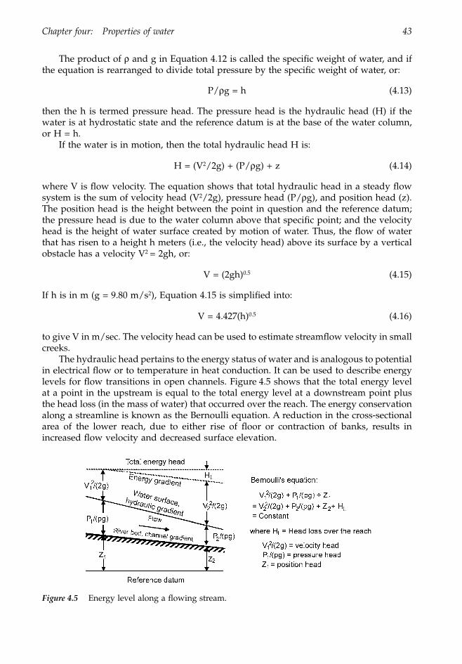
Chapter four: Properties of water 43
The product of r and g in Equation 4.12 is called the specific weight of water, and ifthe equation is rearranged to divide total pressure by the specific weight of water, or:
P/rg = h (4.13)
then the h is termed pressure head. The pressure head is the hydraulic head (H) if thewater is at hydrostatic state and the reference datum is at the base of the water column,or H = h.
If the water is in motion, then the total hydraulic head H is:
H = (V2/2g) + (P/rg) + z (4.14)
where V is flow velocity. The equation shows that total hydraulic head in a steady flowsystem is the sum of velocity head (V2/2g), pressure head (P/rg), and position head (z).The position head is the height between the point in question and the reference datum;the pressure head is due to the water column above that specific point; and the velocityhead is the height of water surface created by motion of water. Thus, the flow of waterthat has risen to a height h meters (i.e., the velocity head) above its surface by a verticalobstacle has a velocity V2 = 2gh, or:
V = (2gh)0.5 (4.15)
If h is in m (g = 9.80 m/s2), Equation 4.15 is simplified into:
V = 4.427(h)0.5 (4.16)
to give V in m/sec. The velocity head can be used to estimate streamflow velocity in smallcreeks.
The hydraulic head pertains to the energy status of water and is analogous to potentialin electrical flow or to temperature in heat conduction. It can be used to describe energylevels for flow transitions in open channels. Figure 4.5 shows that the total energy levelat a point in the upstream is equal to the total energy level at a downstream point plusthe head loss (in the mass of water) that occurred over the reach. The energy conservationalong a streamline is known as the Bernoulli equation. A reduction in the cross-sectionalarea of the lower reach, due to either rise of floor or contraction of banks, results inincreased flow velocity and decreased surface elevation.
Figure 4.5 Energy level along a flowing stream.
1363_C04_fm Page 43 Wednesday, December 4, 2002 7:39 AM
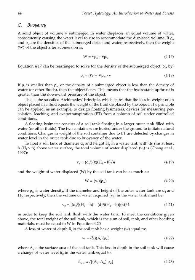
44 Forest Hydrology: An Introduction to Water and Forests
C. Buoyancy
A solid object of volume v submerged in water displaces an equal volume of water,consequently causing the water level to rise to accommodate the displaced volume. If ro
and rw are the densities of the submerged object and water, respectively, then the weight(W) of the object after submersion is:
W = vro - vrw (4.17)
Equation 4.17 can be rearranged to solve for the density of the submerged object, ro, by:
ro = (W + Vrw)/v (4.18)
If ro is smaller than rw, or the density of a submerged object is less than the density ofwater (or other fluids), then the object floats. This means that the hydrostatic upthrust isgreater than the downward pressure of the object.
This is the so-called Archimedes’ Principle, which states that the loss in weight of anobject placed in a fluid equals the weight of the fluid displaced by the object. The principlecan be applied, as an example, to design floating lysimeters, devices for measuring per-colation, leaching, and evapotranspiration (ET) from a column of soil under controlledconditions.
A floating lysimeter consists of a soil tank floating in a larger outer tank filled withwater (or other fluids). The two containers are buried under the ground to imitate naturalconditions. Changes in weight of the soil container due to ET are detected by changes inwater level in the outer tank due to buoyancy of the water.
To float a soil tank of diameter d1 and height H1 in a water tank with its rim at leasth (H1 > h) above water surface, the total volume of water displaced (v1) is (Chang et al.,1997):
v1 = (d12)(p)(H1 – h)/4 (4.19)
and the weight of water displaced (W) by the soil tank can be as much as:
W = (v1)(rw) (4.20)
where rw is water density. If the diameter and height of the outer water tank are d2 andH2, respectively, then the volume of water required (v2) in the water tank must be:
v2 = [(d22)(H2 – h) – (d1
2)(H1 – h)](p)/4 (4.21)
in order to keep the soil tank flush with the water tank. To meet the conditions givenabove, the total weight of the soil tank, which is the sum of soil, tank, and other beddingmaterials, must be equal to W in Equation 4.20.
A loss of water of depth ds in the soil tank has a weight (w) equal to:
w = (ds)(As)(rw) (4.22)
where As is the surface area of the soil tank. This loss in depth in the soil tank will causea change of water level dw in the water tank equal to:
dw = w/[(As+Aw) rw] (4.23)
1363_C04_fm Page 44 Wednesday, December 4, 2002 7:39 AM
Chapter four: Properties of water 45
where Aw is the area of the annular water surface in the water tank. Since the lysimeteris installed under the ground, the gain or loss of water in the water tank is detectedthrough a reservoir connected to the water tank. In this case, the loss of water ds in thesoil tank will cause a change in water level in the reservoir equal to:
dw = (ds)(As)/(As+Aw+Ar) (4.24)
where Ar is the surface area of the reservoir.
D. Surface tension and capillary rise
The force exerted by molecules to bind two different substances in contact together isadhesion, while the force holding molecules of the same substance is cohesion. For exam-ple, when a drop of liquid is placed on a solid surface, the liquid tends to spread out overand wet the surface if the adhesive force between the two substances is greater than thecohesion of the liquid, such as water. On the other hand, the liquid will remain in thedrop form if the adhesive force between the two is smaller than the cohesion of the liquid,such as mercury.
The cohesion of molecules gives a phenomenon at the surface of a liquid called surfacetension. When a liquid is in contact with the wall of a vessel, the edge of this liquid tendsto form considerable curvature due to the inward pull of intermolecular forces. At liq-uid–air interfaces, the molecular attraction for each other at the liquid surface is greaterthan in the air above. This results in an inward force at the liquid surface that acts asthough it has a thin membrane stretched over it. The surface is under tension and con-traction. The force causes the liquid surface to become as small as possible and causes fogdrops, raindrops, and soap bubbles to assume a spherical shape as they fall from the air.
When a fine glass tube is placed in water, water surface rises inside the glass tube.First, adhesion causes water to wet and spread over the glass tube. Then, cohesion causeswater to creep up along the glass wall. The rise will stop when the vertical component ofthe surface tension is equal to the weight of the water raised. This is called capillary action.The height of rise h for any liquid in a capillary tube can be calculated by:
h = 2T/(rrg) (4.25)
where T is the surface tension, r is the radius of the tube, r is the density of the liquid,and g is the force of gravity. For water, T = 73.05 dyn/cm (Table 4.3), Equation 4.24 isreduced to give h in cm per unit area in the simple expression:
h = 0.15/r (4.26)
Table 4.3 Some Physical and Hydraulic Properties of Water, Alcohol, and Mercury
Properties Ethyl Alcohol Water Mercury
Density at 20 ∞C, g cm-3 0.789 0.988 13.55Volume expansion, (10-3) ∞C-1 1.4 0.21 0.18Latent heat of vaporization, cal g–1 at 20∞C 220 586 70.4a
Specific heat, cal g–1∞C-1 0.58 1.00 0.033Surface tension, dyn cm-1 at 20∞C 22.75 73.05 484Heat conductivity, cal sec-1 cm–1 ∞C–1 at 20∞C 0.00040 0.00143 0.0198Viscosity, centipoise at 20∞C 1.200 1.002 1.554
a At boiling point 356.58∞C.
1363_C04_fm Page 45 Wednesday, December 4, 2002 7:39 AM
46 Forest Hydrology: An Introduction to Water and Forests
Surface tension has remarkable effects on water behavior in soils. Water has a T valuehigher than most common liquids. This causes water to be absorbed strongly by capillaryattraction of porous materials, capable of holding water for various purposes.
E. Viscosity
All fluids exhibit, more or less, a property of resistance to changes in shape (or to flow)under the action of external forces. Highly viscous liquids approach solid conditions. Thisis due to the cohesiveness of the molecules in the fluid. According to Newton, the shearstress t at a point within a fluid is proportional to the velocity gradient dv/dz at thatpoint, or:
t = m (dv/dz) (4.27)
where m ( in dyn-sec/cm2 or lb-sec/ft2) is the constant of proportionality known as dynamicor absolute viscosity. Under ordinary conditions, the viscosity of liquids is only affectedby temperature, not by pressure. As temperature increases, gas molecular momentumincreases, and viscosity decreases. For water, a simple way to calculate m by temperatureis (Russell, 1963):
m = , dyn-sec/cm2(4.28)
where T is temperature in °C and m is in dyn-sec/cm2, or g/sec/cm. One dyn-sec/cm2
(or 0.1 Newton-sec/m2) is equal to one poise, in honor of Poiseuille as the unit of viscosityin metric system. One centipoise (cp) is equal to 0.01 poise. Values of the dynamicviscosity for water, alcohol, and mercury are given in Table 4.3. There is no liquid withviscosity as low as that of water, and freshwater is lower than saltwater. As watertemperature decreases, viscosity increases, which causes water to flow slower andrequires more work for wind to produce surface waves, for fish to swim, and for athletesto row a boat.
A parameter often used in fluid motion analyses is the kinematic viscosity n, whichis the ratio of the dynamic viscosity m to the density of the fluid r, or:
n = (4.29)
F. The Reynolds number
The state of flow in an open channel is often described as laminar flow or turbulent flow.When velocity exceeds a critical value, the flow becomes turbulent, chaotic, and disorderly.Otherwise the flow is smooth, calm, and undisturbed. Changes of flow from laminar intoturbulent state depend on the ratio between inertial forces and viscous forces (Albertsonand Simons, 1964). Inertia tends to maintain its speed along a straight line, promotingturbulent conditions, while viscosity dampens disturbances, promoting laminar condi-tions. The Reynolds number (NR) expresses this ratio as follows:
NR = VR/n = rVR/m [Dimensionless] (4.30)
0.01799
1 0.03368T 0.000221T2+ +--------------------------------------------------------------------
mr--- dyne-sec( ) cm 2–
g cm 3–------------------------------------------ dyne-sec-cm
g--------------------------------- cm2 sec 1–= = =
1363_C04_fm Page 46 Wednesday, December 4, 2002 7:39 AM
Chapter four: Properties of water 47
where
V = mean velocity of flow, m/secR = hydraulic radius, mn = kinematic viscosity, m2/sec (m)/(r)r = fluid density, kg/m3
m = dynamic viscosity, N-sec/cm2
When NR £ 500, viscous forces are dominating and the flow is laminar. When NR ≥ 2000,the inertia forces are dominating and the flow is turbulent. The flow in an open channel canbe either laminar or partly turbulent within the transitional range of NR = 500 to 2000 (Chow,1959). The Reynolds number may range from 0.00001 for a bacterium swimming at 0.01mm/sec to 3,000,000,000 for a large whale swimming at 10 m/sec (Vogel, 1994). The Rey-nolds number is highly affected by the size and speed of organisms.
The Reynolds number is of great biological significance, since it affects aquatic speciesdistribution and activity, and the transport of nutrients, energy, and gases to an organism(Gordon et al., 1993; Vogel, 1994). In streamflow measurements with a precalibrated gaug-ing device, maintaining a laminar flow in the approach section is a must for satisfactoryreadings.
G. Shear stress
The forces that moving water exerts on a wetted surface are the tractive force, drag force,and shearing force. They are the components of the weight of water (w) in the directionof flow divided by the area (A) over which they act. Dividing the shearing force by thearea over which it acts is the shear stress. This is the force that causes flow resistance alongthe channel boundary. The stress at which the channel material moves is known as thecritical stress. A greater value of shear stress than critical stress will cause the channel tobe unstable. The shear stress is calculated by:
t = w sin a/A = r · g · V · sin a/At = g · R · S (4.31)
where
t = shear stress (Newton/m2)w = weight of streamflow = r · V· gr = water density (1000 kg/m3 at 4∞Cg = acceleration due to gravity (9.80 m/s2)V = volume of streamflow (m3)a = channel slope (degrees), for small a, sin a ª tan a = SA = channel bed area (m2)R = hydraulic radius (m)
channel cross sectional (m2)/length of wetted perimeter (m)g = specific weight of water = r · g (= 9800 N m–3)S = slope gradient (dimensionless).
The shear stress has been applied extensively to studies in soil erosion, sediment transport,and channel-bank stabilization. More discussion is given in Chapter 11.
1363_C04_fm Page 47 Wednesday, December 4, 2002 7:39 AM

48 Forest Hydrology: An Introduction to Water and Forests
H. Stream power
Another important index for describing the erosive capacity of streams is stream power.Power is the amount of work done per unit of time, and work is the product of forceapplied in the direction of the displacement and the distance of the displacement. Inmathematical form:
Work (w, N-m = joule) = Force (F, Newton) ¥ Distance (D, m) (4.32)
Power (w, J/sec) = Work/Time = N-m/sec = (F)(V) (4.33)
Note that 1 N of force = 1 kg-m/sec2. Expressing stream power as per unit of streambedarea A (m2), then:
w (N/m◊sec = watts/m2) = (F/A)(V) = (t)(V) (4.34)
where t is shear stress in N/m2. Thus, as velocity increases, stream power increases,resulting in a more erosive flow. A flash flood in steep, mountainous areas can generatevalues of stream power much greater than major rivers.
In his sediment-transport study, Bagnold (1966) expressed stream power as the rateof potential energy over a unit length of stream channel:
wL = rgQS (4.35)
where Q = the whole discharge of the stream (m3/sec), S = the energy slope of the channel(dimensionless), r and g are defined in Equation 4.31, and wL = stream power in unitlength (N-m/sec3, or watts/m). The whole available power (wL) supply to the column ofwater over unit bed area is the w in Equation 4.34 or:
(4.36)
where d is the average depth in m and can be used to substitute the hydraulic radius R.
III. Chemical propertiesA. The water molecule
A water molecule is made of one electronegative oxygen (O-) atom and two much smallerelectropositive hydrogen (H+) atoms. Each atom consists of electrons in negative chargeand a nucleus in positive charge. Electrons circle around the central nucleus. The numberof electrons in an atom, the atomic number, varies among elements. There are eightelectrons in an oxygen atom and one electron in a hydrogen atom.
There are two types of chemical bonds in water: covalent bonds and hydrogen bonds.Each H atom in a water molecule is attached to the O atom by a single covalent bond.Thus, the three atoms are held together by two covalent bonds. Oxygen is the second mostelectronegative element. As a result, the two covalent bonds in water are polar and arestructured in a V shape of 105°. The polarization makes a partial negative charge on theoxygen atom and a partial positive charge on each hydrogen atom, which is responsiblefor many of water’s unique properties, such as its being an excellent solvent.
w = wL
flow width----------------------------- rgQS
flow width----------------------------- rgS
m3 sec 1–
m---------------------
Ë ¯Ê � rgS(dV) = (rgSd) (V) = tV= = =
1363_C04_fm Page 48 Wednesday, December 4, 2002 7:39 AM
Chapter four: Properties of water 49
Hydrogen bonds are intermolecular bonds, or bonds between atoms in differentmolecules formed by electrostatic attraction. Each oxygen atom in water can form twohydrogen bonds, one through each of the unbounded pairs of electrons. Thus, each watermolecule is linked to others through intermolecular hydrogen bonds to form a three-dimensional aggregate of water molecules (Buchan, 1996). The bonds give water a muchlarger and heavier molecule and explain in part its relatively higher melting point, boilingpoint, heat of fusion, and heat of vaporization.
B. Formation of water
Water is formed when hydrogen is burned in air. However, the ignition will cause anexplosion if it occurs on hydrogen mixed with air or oxygen:
2 H2 + O2 Æ 2 H2O + 115.6 kcal
Other reactions that produce water include the process of respiration in the cells andorgans of living plants:
C12H6O12 + O2 Æ 6 CO2 + H2O + 673 kcal
neutralization of acid and base:
H2SO4 + 2 NaOH Æ Na2SO4 + 2 H2O
and combustion of hydrogen-containing materials:
CH4 + 2 O2 Æ CO2 + 2 H2O + 192 kcal
C. Chemical reactions
Water molecules are very stable with respect to heat. Water decomposes into its elementsto the extent of about 1% at temperatures up to 2000∞C. However, water reacts with manyelements, including metals, nonmetals, and metal and nonmetal oxides, or it may becomea part of the crystalline structure of compounds known as hydrates through the processof hydration (Hein, 1990)
The reaction of water with metals may take place at cold temperatures, such as calciumsinks in water, to form calcium hydroxides and liberate a gentle stream of hydrogen:
Ca (Solid) + 2 H2O (Liquid) Æ H2≠ + Ca(OH)2
or at high temperatures, such as zinc and water, to form oxidized zinc:
Zn (Solid) + H2O (steam) Æ H2≠ + ZnO (solid)
Metal oxides known as basic anhydrides react with water to form basic anhydrides, suchas:
CaO (Solid) + H2O Æ Ca(OH)2 (Calcium hydroxide)
1363_C04_fm Page 49 Wednesday, December 4, 2002 7:39 AM
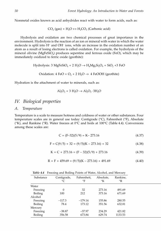
50 Forest Hydrology: An Introduction to Water and Forests
Nonmetal oxides known as acid anhydrides react with water to form acids, such as:
CO2 (gas) + H2O ´ H2CO3 (Carbonic acid)
Hydrolysis and oxidation are two chemical processes of great importance in theenvironment. Hydrolysis is the reaction of an ion or mineral with water in which the watermolecule is split into H+ and OH- ions, while an increase in the oxidation number of anatom as a result of losing electrons is called oxidation. For example, the hydrolysis of themineral olivine (MgFeSiO4) produces sepentine and ferrous oxide (FeO), which may beimmediately oxidized to ferric oxide (geothite):
Hydrolysis: 3 MgFeSiO4 + 2 H2O Æ H4Mg3Si2O9 + SiO2 +3 FeO
Oxidation: 4 FeO + O2 + 2 H2O Æ 4 FeOOH (geothite)
Hydration is the attachment of water to minerals, such as:
Al2O3 + 3 H2O Æ Al2O3 · 3H2O
IV. Biological properties
A. Temperature
Temperature is a scale to measure hotness and coldness of water or other substances. Fourtemperature scales are in general use today: Centigrade (∞C), Fahrenheit (∞F), Absolute(∞K), and Rankine (∞R). Water freezes at 0∞C and boils at 100∞C (Table 4.4). Conversionsamong these scales are:
C = (F–32)(5/9) = K– 273.16 (4.37)
F = C(9/5) + 32 = (9/5)(K – 273.16) + 32 (4.38)
K = C + 273.16 = (F – 32)(5/9) + 273.16 (4.39)
R = F + 459.69 = (9/5)(K – 273.16) + 491.69 (4.40)
Table 4.4 Freezing and Boiling Points of Water, Alcohol, and Mercury
Substance Centigrade, °C
Fahrenheit, °F
Absolute, °K
Rankine, °R
WaterFreezing 0 32 273.16 491.69Boiling 100 212 373.16 671.69
AlcoholFreezing -117.3 -179.14 155.86 280.55Boiling 78.4 173.12 351.56 632.81
MercuryFreezing -38.87 –37.97 234.29 421.82Boiling 356.58 673.84 629.74 1133.53
1363_C04_fm Page 50 Wednesday, December 4, 2002 7:39 AM
Chapter four: Properties of water 51
The main sources of heat for streams and reservoirs are solar radiation (Rs), longwaveradiation from the atmosphere (Ra), the energy advected into the body of water by pre-cipitation and inflow (Ri), and the conducted heat from the ground (Rc). However, heatalso can be lost from water to the environment through surface reflection of solar radiation(Rr), longwave radiation or sensible heat to the atmosphere (Rw), and latent heat of vapor-ization (Rv). The difference between heat gain and heat loss is balanced by a positive ornegative term of heat storage, Rst, by the following equation:
(Rs + Ra+Ri + Rc) - (Rr + Rw + Rv) ± Rst = 0 (4.41)
Thus, water temperature will increase or decrease in response to the positive or negativevalue of Rst. In small forested streams, the exposure of stream channel to direct solarradiation due to clearcutting of riparian vegetation may cause an increase in streamtemperature adversely affecting aquatic ecosystems. Stream and lake waters are often usedin industrial cooling processes. Hot water discharged into streams from a power plantmay raise the temperature of water enough to produce major changes in aquatic commu-nities. The effect of thermal discharge of power plants on stream temperature can becalculated by the following mixing equation:
Td = (4.42)
where T is temperature, Q is flow rate, and subscripts p, m, and d refer to power plant,upstream, and downstream, respectively.
Water temperature is a primary factor affecting physical and chemical properties ofwater, including the rate of chemical reaction, gas solubility, decomposition of organicmatter, latent heat, saturation vapor pressure, changes in the state of water, water density,viscosity, heat conduction, velocity of particle settlement, water circulation, and others. Italso regulates biological activities in the aquatic environment. Cool water is always betterin quality than warm water because of higher concentration of dissolved oxygen andlower rates of microbial activities, organic matter decomposition, and chemical reaction.
The internal temperature for most aquatic animals follows closely with water temper-ature. As a rule of thumb, an increase in temperature 10∞C doubles the metabolic rate ofcold-blooded organisms and the rate of chemical reactions. The optimum temperaturerange for aquatic organisms varies with species and the life stage of each species. Changesin temperature of only a few degrees can adversely affect the production, growth, devel-opment, and survival of an organism. The optimum temperature range for most salmonspecies is about 12 to 14∞C, and the lethal level for adults is about 20 to 25∞C, dependingon duration and rate of the temperature increase. Some salmon eggs and juveniles maybe killed at 13.5∞C (MacDonald et al., 1991).
B. Dissolved oxygen
Dissolved oxygen (DO) refers to the amount of oxygen dissolved in water and is expressedin ppm or mg/liter. The concentration of DO in stream water is determined by the oxygen-holding ability, oxygen depletion, and oxygen replenishment of the stream. Oxygen dis-solves in water through diffusion at the interface between water and air. The solubility ofoxygen in water is inversely proportional to water temperature and increases with increas-ing atmospheric pressure (Figure 4.6). At one standard atmospheric pressure (760 mm Hg),
Tp( ) Qp( ) Tm( ) Qm( )+Qp Qm+
-----------------------------------------------------
1363_C04_fm Page 51 Wednesday, December 4, 2002 7:39 AM
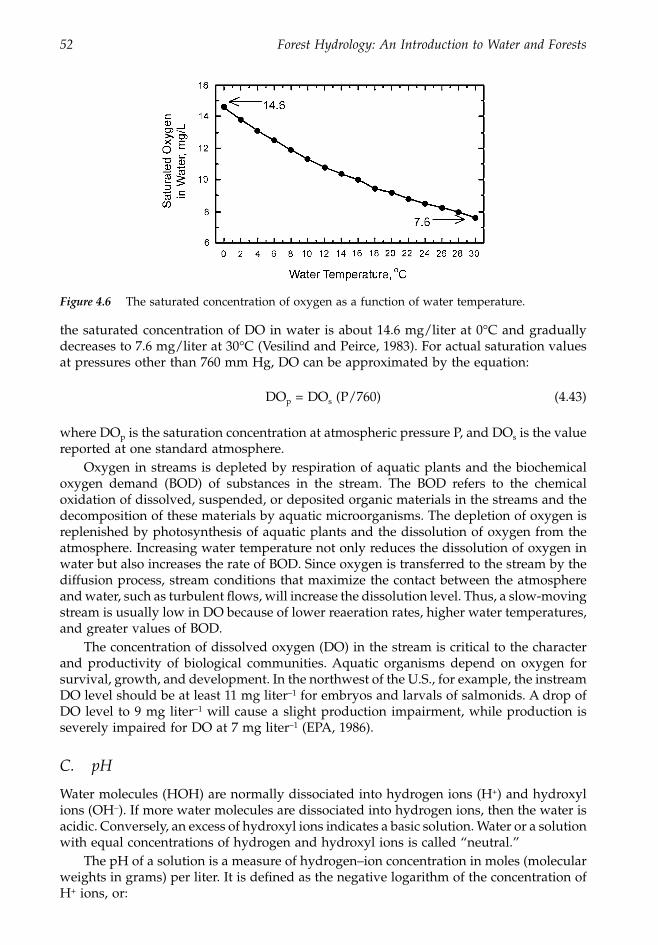
52 Forest Hydrology: An Introduction to Water and Forests
the saturated concentration of DO in water is about 14.6 mg/liter at 0∞C and graduallydecreases to 7.6 mg/liter at 30∞C (Vesilind and Peirce, 1983). For actual saturation valuesat pressures other than 760 mm Hg, DO can be approximated by the equation:
DOp = DOs (P/760) (4.43)
where DOp is the saturation concentration at atmospheric pressure P, and DOs is the valuereported at one standard atmosphere.
Oxygen in streams is depleted by respiration of aquatic plants and the biochemicaloxygen demand (BOD) of substances in the stream. The BOD refers to the chemicaloxidation of dissolved, suspended, or deposited organic materials in the streams and thedecomposition of these materials by aquatic microorganisms. The depletion of oxygen isreplenished by photosynthesis of aquatic plants and the dissolution of oxygen from theatmosphere. Increasing water temperature not only reduces the dissolution of oxygen inwater but also increases the rate of BOD. Since oxygen is transferred to the stream by thediffusion process, stream conditions that maximize the contact between the atmosphereand water, such as turbulent flows, will increase the dissolution level. Thus, a slow-movingstream is usually low in DO because of lower reaeration rates, higher water temperatures,and greater values of BOD.
The concentration of dissolved oxygen (DO) in the stream is critical to the characterand productivity of biological communities. Aquatic organisms depend on oxygen forsurvival, growth, and development. In the northwest of the U.S., for example, the instreamDO level should be at least 11 mg liter-1 for embryos and larvals of salmonids. A drop ofDO level to 9 mg liter-1 will cause a slight production impairment, while production isseverely impaired for DO at 7 mg liter-1 (EPA, 1986).
C. pH
Water molecules (HOH) are normally dissociated into hydrogen ions (H+) and hydroxylions (OH-). If more water molecules are dissociated into hydrogen ions, then the water isacidic. Conversely, an excess of hydroxyl ions indicates a basic solution. Water or a solutionwith equal concentrations of hydrogen and hydroxyl ions is called “neutral.”
The pH of a solution is a measure of hydrogen–ion concentration in moles (molecularweights in grams) per liter. It is defined as the negative logarithm of the concentration ofH+ ions, or:
Figure 4.6 The saturated concentration of oxygen as a function of water temperature.
1363_C04_fm Page 52 Wednesday, December 4, 2002 7:39 AM
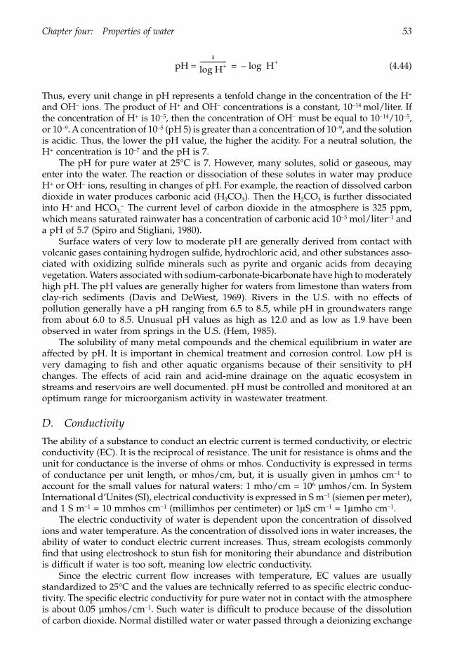
Chapter four: Properties of water 53
(4.44)
Thus, every unit change in pH represents a tenfold change in the concentration of the H+
and OH- ions. The product of H+ and OH- concentrations is a constant, 10-14 mol/liter. Ifthe concentration of H+ is 10-5, then the concentration of OH- must be equal to 10-14/10-5,or 10-9. A concentration of 10-5 (pH 5) is greater than a concentration of 10-9, and the solutionis acidic. Thus, the lower the pH value, the higher the acidity. For a neutral solution, theH+ concentration is 10-7 and the pH is 7.
The pH for pure water at 25°C is 7. However, many solutes, solid or gaseous, mayenter into the water. The reaction or dissociation of these solutes in water may produceH+ or OH- ions, resulting in changes of pH. For example, the reaction of dissolved carbondioxide in water produces carbonic acid (H2CO3). Then the H2CO3 is further dissociatedinto H+ and HCO3.
- The current level of carbon dioxide in the atmosphere is 325 ppm,which means saturated rainwater has a concentration of carbonic acid 10-5 mol/liter-1 anda pH of 5.7 (Spiro and Stigliani, 1980).
Surface waters of very low to moderate pH are generally derived from contact withvolcanic gases containing hydrogen sulfide, hydrochloric acid, and other substances asso-ciated with oxidizing sulfide minerals such as pyrite and organic acids from decayingvegetation. Waters associated with sodium-carbonate-bicarbonate have high to moderatelyhigh pH. The pH values are generally higher for waters from limestone than waters fromclay-rich sediments (Davis and DeWiest, 1969). Rivers in the U.S. with no effects ofpollution generally have a pH ranging from 6.5 to 8.5, while pH in groundwaters rangefrom about 6.0 to 8.5. Unusual pH values as high as 12.0 and as low as 1.9 have beenobserved in water from springs in the U.S. (Hem, 1985).
The solubility of many metal compounds and the chemical equilibrium in water areaffected by pH. It is important in chemical treatment and corrosion control. Low pH isvery damaging to fish and other aquatic organisms because of their sensitivity to pHchanges. The effects of acid rain and acid-mine drainage on the aquatic ecosystem instreams and reservoirs are well documented. pH must be controlled and monitored at anoptimum range for microorganism activity in wastewater treatment.
D. Conductivity
The ability of a substance to conduct an electric current is termed conductivity, or electricconductivity (EC). It is the reciprocal of resistance. The unit for resistance is ohms and theunit for conductance is the inverse of ohms or mhos. Conductivity is expressed in termsof conductance per unit length, or mhos/cm, but, it is usually given in µmhos cm-1 toaccount for the small values for natural waters: 1 mho/cm = 106 µmhos/cm. In SystemInternational d’Unites (SI), electrical conductivity is expressed in S m-1 (siemen per meter),and 1 S m-1 = 10 mmhos cm-1 (millimhos per centimeter) or 1mS cm-1 = 1mmho cm-1.
The electric conductivity of water is dependent upon the concentration of dissolvedions and water temperature. As the concentration of dissolved ions in water increases, theability of water to conduct electric current increases. Thus, stream ecologists commonlyfind that using electroshock to stun fish for monitoring their abundance and distributionis difficult if water is too soft, meaning low electric conductivity.
Since the electric current flow increases with temperature, EC values are usuallystandardized to 25∞C and the values are technically referred to as specific electric conduc-tivity. The specific electric conductivity for pure water not in contact with the atmosphereis about 0.05 µmhos/cm-1. Such water is difficult to produce because of the dissolutionof carbon dioxide. Normal distilled water or water passed through a deionizing exchange
pH = 1
log H+----------------- log H+–=
1363_C04_fm Page 53 Wednesday, December 4, 2002 7:39 AM
54 Forest Hydrology: An Introduction to Water and Forests
unit usually has a conductivity of at least 1 µmho cm-1. Seawater has a concentration ofdissolved solids of about 35,000 mg/liter-1; thus, its conductivity is about 50,000 µmhoscm-1.
Conductivity is often used as a parameter to determine the suitability of water for aspecific purpose such as food preparation, agricultural irrigation, and water supply; totest the result of wastewater treatment; or to control water quality and other manufacturingprocesses. In soils, conductivity is higher on clays and lower on sands. Many soil propertiessuch as texture, subsoil characteristics, salinity, cation exchange capacity, level of organicmatter, and drainage conditions can be related to EC.
E. Sediment
Stream sediments are particles, usually inorganic, released from land surfaces or streambanks by the action of raindrops, gravity, animals, overland flows, and streamflows. Theycan be in suspension (no contact with streambed), saltation (bouncing along streambed),and bed-load (rolling along streambed). No streams are free from sediments. Expressedin ppm or mg/liter-1, the concentration of sediment is affected by environmental condi-tions of the watershed such as geology, soil, topography, climate, vegetation cover, andland-use activity. Sometimes, the amount of stream sediment is expressed in terms ofturbidity. Turbidity is an optical measure either in Jackson turbidity units (JTU; one suchunit is the turbidity produced by 1 ppm of silica in distilled water) or nephelometricturbidity units (NTU, comparable to Jackson units). It measures the clarity of water asaffected by light attenuation of suspended particles (Davies-Colley and Smith, 2001). Sincethe optical property of water samples is greatly affected by the size, shape, configuration,color, and origin of particles, the correlation between JTU and the weight of sedimentsper unit volume of water is valid only through local calibration.
Sediment concentration has tremendous impacts on the physical and chemical prop-erties of water and consequently affects lives in the aquatic environment. Physically,sediments affect water turbidity, odor, taste, temperature regime, and abrasiveness; reducelight penetration; increase solar absorption at water surface; deplete reservoir capacity;and clog stream channels. Recreational and aesthetic values of streams can be impairedand turbines in hydroelectric plants can be damaged because of sediment.
Sometimes sediment concentration is weighed by flow volume to obtain sedimentloss in mass per unit time and per unit watershed area. It is also referred to as sedimentyield or sediment load. Generally, watershed area has a negative effect on sediment loss.This may be attributable to the fact that a small watershed is generally associated withless watershed storage, greater rainfall intensity and depth, steeper mean watershed slope,and greater chance for the entire watershed to be covered by a storm.
Sediments can carry many elements and compounds that may interact with oneanother in water, consequently affecting water chemistry and quality (Tessier, 1992). Thenature and content of these compounds and elements resemble the origin of soil particlesplus the residuals from applications of fertilizers, insecticides, herbicides, industrialwastes, fallout from air pollution, and decomposition of organic matter. Concentration ofsediment in streams is often highly correlated with nutrient concentration and can be usedto estimate nutrient losses in streams (Chang et al., 1983; Granillo et al., 1985).
The effects of stream sediment on aquatic ecosystems can be direct through its presenceor indirect through interactions with the physical and chemical environment of the stream.Streams with sandy beds have the lowest species diversity and aquatic productivity. Thehabitat space for small fish, invertebrates, and other organisms can be reduced if theinterstices between coarse particles are filled by fine sediments (MacDonald et al., 1991).Photosynthesis of aquatic plants can be inhibited because of the reduction of light pene-
1363_C04_fm Page 54 Wednesday, December 4, 2002 7:39 AM
Chapter four: Properties of water 55
tration. This may lead to declines in foods along the aquatic food chain. In addition,increases in absorption of solar radiation at the water surface may raise water temperature,which will lead to declines in dissolved oxygen for aquatic life consumption.
ReferencesAlbertson, M.L. and Simons, D.B., 1964, Fluid mechanics, in Handbook of Applied Hydrology, Chow,
V.T., Ed., McGraw-Hill, New York, pp. 7:1–49.Bagnold, R.A., 1966, An Approach to the Sediment Transport Problem from General Physics., U.S.
Geological Survey Professional Paper, 422-I. Buchan, G.D., 1996, Ode to H2O, J. Soil Water Conser., 51, 467–470.Chang, M., McCullough, J.D., and Granillo, A.B., 1983, Effects of land use and topography on some
water quality variables in forested East Texas, Water Resour. Bull., 19, 191–196.Chang, M. et al., 1997, Evapotranspiration of herbaceous mimosa (Mimosa strigillosa), a new
drought-resistant species in the southeastern United States, Resour., Conserv. and Recycling,21, 175–184.
Chow, V.T., 1959, Open Channel Hydraulics, McGraw-Hill, New York. Davies-Colley, R.J. and Smith, D.G., 2001, Turbidity, suspended sediment, and water clarity: a review,
J. Am. Water Resour. Assoc., 37, 1085–1101.Davis, S.N. and DeWiest, R.J.M., 1969, Hydrogeology, John Wiley & Sons, New York.der Leeden, F.V., Troise, F.L., and Todd, D.K., 1990, The Water Encyclopedia, Lewis Publishers, Chelsea,
MI.EPA, 1986, Ambient Water Quality Criteria for Dissolved Oxygen, U.S. Environmental Protection
Agency, Office of Water Regulations and Standards, Washington, D.C.Gordon, N.D., McMahon, T.A., and Finlayson, B.L., 1993, Stream Hydrology, an Introduction for Ecol-
ogists, John Wiley & Sons, New York.Granillo, A.B., Chang, M., and Rashin, E.B., 1985, Correlation between suspended sediment and
some water quality parameters in small streams of forested East Texas, Texas J. Sci., 37,227–234.
Hein, M., 1990, Foundations of College Chemistry, Brooks/Cole, Pacific Grove, CA.Hem, J.D., 1985, Study and Interpretation of the Chemical Characteristics of Natural Water, 3rd Ed., U.S.
Geological Survey Water Supply Paper 2254.List, R.J., 1971, Smithsonian Meteorological Tables, 6th rev. ed., Smithsonian Institute Press, Washington,
D.C. MacDonald, L.H., Smart, A.W., and Wisssmar, R.C., 1991. Monitoring Guidelines to Evaluate Effects
of Forestry Activities on Streams in the Pacific Northwest and Alaska, EPA/910/91–001, U.S.Environmental Protection Agency, Region 10, Seattle, WA.
Spiro, T.G. and Stigliani, W.M., 1980, Environmental Science in Perspective, State University of NewYork Press, Albany, NY.
Tabata, S., 1973, A simple but accurate formula for the saturation vapor pressure over liquid water,J. Appl. Meteorol., 12, 1410–11.
Tessier, A., 1992, Sorption of trace elements on natural particles in oxic environments, in Environ-mental Particles, Lewis Publishers, Boca Raton, FL, pp. 425–453.
Vesilind, P.A. and Peirce, J.J., 1983, Environmental Pollution and Control, Ann Arbor Science, AnnArbor, MI.
Vogel, S., 1994, Life in Moving Fluids, the Physical Biology of Flow, Princeton University Press, Princeton,NJ.
1363_C04_fm Page 55 Wednesday, December 4, 2002 7:39 AM

1363_C04_fm Page 56 Wednesday, December 4, 2002 7:39 AM

57
chapter five
Water distribution
Contents
I. The globe ............................................................................................................................58A. Saline water ...............................................................................................................58B. Freshwater..................................................................................................................59
1. Icecaps and glaciers............................................................................................602. Water under the ground ....................................................................................613. Lakes .....................................................................................................................624. Rivers ....................................................................................................................625. Atmospheric water .............................................................................................62
II. The U.S................................................................................................................................62A. Rivers ..........................................................................................................................63B. Lakes ...........................................................................................................................64
III. The hydrologic cycle.........................................................................................................65A. The hydrologic processes ........................................................................................66
1. Precipitation.........................................................................................................662. Evapotranspiration .............................................................................................673. Runoff ...................................................................................................................67
B. The hydrologic budget.............................................................................................671. The globe..............................................................................................................672. The U.S. ................................................................................................................683. Watersheds ...........................................................................................................69
C. The energy budget....................................................................................................70References .......................................................................................................................................72
Earth is the only planet in the solar system where water appears in solid, liquid, and vaporstates at common temperatures. The existence of water on Earth has a lot to do with Earth’ssize and distance from the Sun. Hydrogen (90%), helium (9%), and oxygen are the threemost abundant elements in the universe, followed by neon, nitrogen, and carbon (Cox,1989). Helium and neon are solitary elements. Thus, two hydrogens and one oxygen atomare easily bound to become water (H
2
O), three hydrogens join one nitrogen to becomeammonia (NH
3
), and four hydrogens join one carbon to become methane (CH
4
). Themelting points of H
2
O, NH
3
, and CH
4
are 0
∞
C,
-
78
∞
C, and
-
183
∞
C, respectively, while theboiling points are 100
∞
C,
-
33
∞
C, and
-
162
∞
C. The average surface temperature of Earth isabout 27
∞
C, sufficient to keep water in liquid state.
1363_C05_fm Page 57 Wednesday, December 4, 2002 7:40 AM
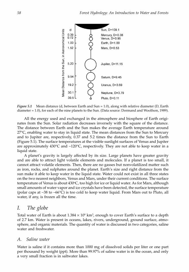
58 Forest Hydrology: An Introduction to Water and Forests
All the energy used and exchanged in the atmosphere and biosphere of Earth origi-nates from the Sun. Solar radiation decreases inversely with the square of the distance.The distance between Earth and the Sun makes the average Earth temperature around27
∞
C, enabling water to stay in liquid state. The mean distances from the Sun to Mercuryand to Jupiter are, respectively, 0.37 and 5.2 times the distance from the Sun to Earth(Figure 5.1). The surface temperatures at the visible sunlight surfaces of Venus and Jupiterare approximately 430
∞
C and
-
120
∞
C, respectively. They are not able to keep water in aliquid state.
A planet’s gravity is largely affected by its size. Large planets have greater gravityand are able to attract light volatile elements and molecules. If a planet is too small, itcannot attract volatile elements. Then, there are no gasses but nonvolatilized matter suchas iron, rocks, and sulphates around the planet. Earth’s size and right distance from thesun make it able to keep water in the liquid state. Water could not exist in all three stateson the two nearest neighbors, Venus and Mars, under their current conditions. The surfacetemperature of Venus is about 430
o
C, too high for ice or liquid water. As for Mars, althoughsmall amounts of water vapor and ice crystals have been detected, the surface temperature(polar caps at
-
38 to
-
66
∞
C) is too cold to keep water liquid. From Mars out to Pluto, allwater, if any, is frozen all the time.
I. The globe
Total water of Earth is about 1.384
¥
10
9
km
3
, enough to cover Earth’s surface to a depthof 2.7 km. Water is present in oceans, lakes, rivers, underground, ground surface, atmo-sphere, and organic materials. The quantity of water is discussed in two categories, salinewater and freshwater.
A. Saline water
Water is saline if it contains more than 1000 mg of dissolved solids per liter or one partper thousand by weight (ppt). More than 99.97% of saline water is in the ocean, and onlya very small fraction is in saltwater lakes.
Figure 5.1
Mean distance (d, between Earth and Sun = 1.0), along with relative diameter (D, Earthdiameter = 1.0), for each of the nine planets to the Sun. (Data source: Dormand and Woolfson, 1989).
1363_C05_fm Page 58 Wednesday, December 4, 2002 7:40 AM
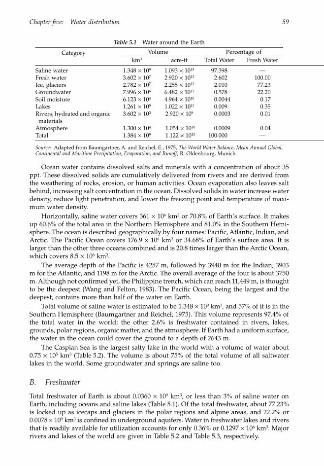
Chapter five: Water distribution 59
Ocean water contains dissolved salts and minerals with a concentration of about 35ppt. These dissolved solids are cumulatively delivered from rivers and are derived fromthe weathering of rocks, erosion, or human activities. Ocean evaporation also leaves saltbehind, increasing salt concentration in the ocean. Dissolved solids in water increase waterdensity, reduce light penetration, and lower the freezing point and temperature of maxi-mum water density.
Horizontally, saline water covers 361
¥
10
6
km
2
or 70.8% of Earth’s surface. It makesup 60.6% of the total area in the Northern Hemisphere and 81.0% in the Southern Hemi-sphere. The ocean is described geographically by four names: Pacific, Atlantic, Indian, andArctic. The Pacific Ocean covers 176.9
¥
10
6
km
2
or 34.68% of Earth’s surface area. It islarger than the other three oceans combined and is 20.8 times larger than the Arctic Ocean,which covers 8.5
¥
10
6
km
2
.The average depth of the Pacific is 4257 m, followed by 3940 m for the Indian, 3903
m for the Atlantic, and 1198 m for the Arctic. The overall average of the four is about 3750m. Although not confirmed yet, the Philippine trench, which can reach 11,449 m, is thoughtto be the deepest (Wang and Felton, 1983). The Pacific Ocean, being the largest and thedeepest, contains more than half of the water on Earth.
Total volume of saline water is estimated to be 1.348
¥
10
9
km
3
, and 57% of it is in theSouthern Hemisphere (Baumgartner and Reichel, 1975). This volume represents 97.4% ofthe total water in the world; the other 2.6% is freshwater contained in rivers, lakes,grounds, polar regions, organic matter, and the atmosphere. If Earth had a uniform surface,the water in the ocean could cover the ground to a depth of 2643 m.
The Caspian Sea is the largest salty lake in the world with a volume of water about0.75
¥
10
5
km
3
(Table 5.2). The volume is about 75% of the total volume of all saltwaterlakes in the world. Some groundwater and springs are saline too.
B. Freshwater
Total freshwater of Earth is about 0.0360
¥
10
9
km
3
, or less than 3% of saline water onEarth, including oceans and saline lakes (Table 5.1). Of the total freshwater, about 77.23%is locked up as icecaps and glaciers in the polar regions and alpine areas, and 22.2% or0.0078
¥
10
9
km
3
is confined in underground aquifers. Water in freshwater lakes and riversthat is readily available for utilization accounts for only 0.36% or 0.1297
¥
10
6
km
3
. Majorrivers and lakes of the world are given in Table 5.2 and Table 5.3, respectively.
Table 5.1
Water around the Earth
Category
Volume
Percentage ofkm
3
acre-ft Total Water Fresh Water
Saline water 1.348
¥
10
9
1.093
¥
10
15
97.398 —Fresh water 3.602
¥
10
7
2.920
¥
10
13
2.602 100.00Ice, glaciers 2.782
¥
10
7
2.255
¥
10
13
2.010 77.23Groundwater 7.996
¥
10
6
6.482
¥
10
12
0.578 22.20Soil moisture 6.123
¥
10
4
4.964
¥
10
10
0.0044 0.17Lakes 1.261
¥
10
5
1.022
¥
10
11
0.009 0.35Rivers; hydrated and organic materials
3.602
¥
10
3
2.920
¥
10
9
0.0003 0.01
Atmosphere 1.300
¥
10
4
1.054
¥
10
10
0.0009 0.04Total 1.384
¥
10
9
1.122
¥
10
15
100.000 —
Source:
Adapted from Baumgartner, A. and Reichel, E., 1975,
The World Water Balance, Mean Annual Global,Continental and Maritime Precipitation, Evaporation, and Runoff
, R. Oldenbourg, Munich.
1363_C05_fm Page 59 Wednesday, December 4, 2002 7:40 AM
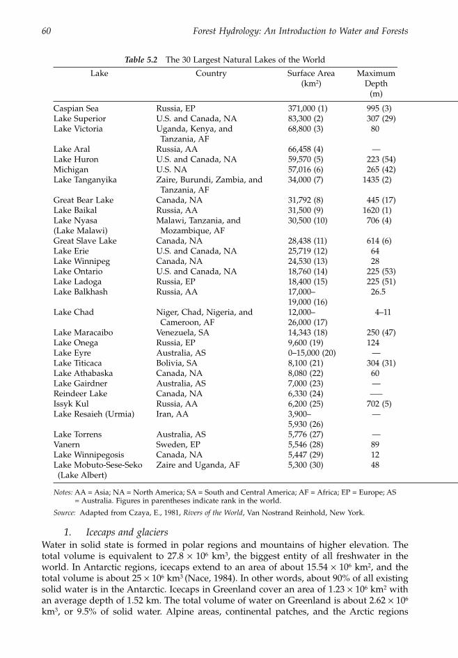
60 Forest Hydrology: An Introduction to Water and Forests
1. Icecaps and glaciers
Water in solid state is formed in polar regions and mountains of higher elevation. Thetotal volume is equivalent to 27.8
¥
10
6
km
3
, the biggest entity of all freshwater in theworld. In Antarctic regions, icecaps extend to an area of about 15.54
¥
10
6
km
2
, and thetotal volume is about 25
¥
10
6
km
3
(Nace, 1984). In other words, about 90% of all existingsolid water is in the Antarctic. Icecaps in Greenland cover an area of 1.23
¥
10
6
km
2
withan average depth of 1.52 km. The total volume of water on Greenland is about 2.62
¥
10
6
km
3
, or 9.5% of solid water. Alpine areas, continental patches, and the Arctic regions
Table 5.2
The 30 Largest Natural Lakes of the World
Lake Country Surface Area(km
2
) Maximum
Depth(m)
Caspian Sea Russia, EP 371,000 (1) 995 (3)Lake Superior U.S. and Canada, NA 83,300 (2) 307 (29)Lake Victoria Uganda, Kenya, and
Tanzania, AF68,800 (3) 80
Lake Aral Russia, AA 66,458 (4) —Lake Huron U.S. and Canada, NA 59,570 (5) 223 (54)Michigan U.S. NA 57,016 (6) 265 (42)Lake Tanganyika Zaire, Burundi, Zambia, and
Tanzania, AF34,000 (7) 1435 (2)
Great Bear Lake Canada, NA 31,792 (8) 445 (17)Lake Baikal Russia, AA 31,500 (9) 1620 (1)Lake Nyasa(Lake Malawi)
Malawi, Tanzania, and Mozambique, AF
30,500 (10) 706 (4)
Great Slave Lake Canada, NA 28,438 (11) 614 (6)Lake Erie U.S. and Canada, NA 25,719 (12) 64Lake Winnipeg Canada, NA 24,530 (13) 28Lake Ontario U.S. and Canada, NA 18,760 (14) 225 (53)Lake Ladoga Russia, EP 18,400 (15) 225 (51)Lake Balkhash Russia, AA 17,000–
19,000 (16)26.5
Lake Chad Niger, Chad, Nigeria, and Cameroon, AF
12,000–26,000 (17)
4–11
Lake Maracaibo Venezuela, SA 14,343 (18) 250 (47)Lake Onega Russia, EP 9,600 (19) 124Lake Eyre Australia, AS 0–15,000 (20) —Lake Titicaca Bolivia, SA 8,100 (21) 304 (31)Lake Athabaska Canada, NA 8,080 (22) 60Lake Gairdner Australia, AS 7,000 (23) —Reindeer Lake Canada, NA 6,330 (24) –—Issyk Kul Russia, AA 6,200 (25) 702 (5)Lake Resaieh (Urmia) Iran, AA 3,900–
5,930 (26)—
Lake Torrens Australia, AS 5,776 (27) —Vanern Sweden, EP 5,546 (28) 89Lake Winnipegosis Canada, NA 5,447 (29) 12Lake Mobuto-Sese-Seko (Lake Albert)
Zaire and Uganda, AF 5,300 (30) 48
Notes:
AA = Asia; NA = North America; SA = South and Central America; AF = Africa; EP = Europe; AS= Australia. Figures in parentheses indicate rank in the world.
Source:
Adapted from Czaya, E., 1981,
Rivers of the World
, Van Nostrand Reinhold, New York.
1363_C05_fm Page 60 Wednesday, December 4, 2002 7:40 AM
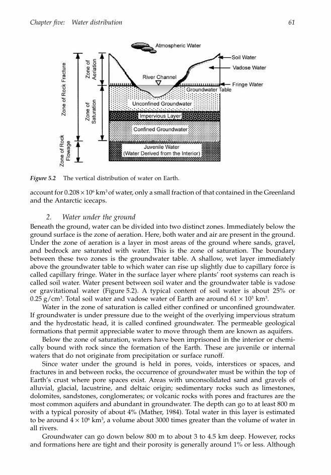
Chapter five: Water distribution 61
account for 0.208
¥
10
6
km
3
of water, only a small fraction of that contained in the Greenlandand the Antarctic icecaps.
2. Water under the ground
Beneath the ground, water can be divided into two distinct zones. Immediately below theground surface is the zone of aeration. Here, both water and air are present in the ground.Under the zone of aeration is a layer in most areas of the ground where sands, gravel,and bedrock are saturated with water. This is the zone of saturation. The boundarybetween these two zones is the groundwater table. A shallow, wet layer immediatelyabove the groundwater table to which water can rise up slightly due to capillary force iscalled capillary fringe. Water in the surface layer where plants’ root systems can reach iscalled soil water. Water present between soil water and the groundwater table is vadoseor gravitational water (Figure 5.2). A typical content of soil water is about 25% or0.25 g/cm
3
.
Total soil water and vadose water of Earth are around 61
¥
10
3
km
3
.Water in the zone of saturation is called either confined or unconfined groundwater.
If groundwater is under pressure due to the weight of the overlying impervious stratumand the hydrostatic head, it is called confined groundwater. The permeable geologicalformations that permit appreciable water to move through them are known as aquifers.
Below the zone of saturation, waters have been imprisoned in the interior or chemi-cally bound with rock since the formation of the Earth. These are juvenile or internalwaters that do not originate from precipitation or surface runoff.
Since water under the ground is held in pores, voids, interstices or spaces, andfractures in and between rocks, the occurrence of groundwater must be within the top ofEarth’s crust where pore spaces exist. Areas with unconsolidated sand and gravels ofalluvial, glacial, lacustrine, and deltaic origin; sedimentary rocks such as limestones,dolomites, sandstones, conglomerates; or volcanic rocks with pores and fractures are themost common aquifers and abundant in groundwater. The depth can go to at least 800 mwith a typical porosity of about 4% (Mather, 1984). Total water in this layer is estimatedto be around 4
¥
10
6
km3, a volume about 3000 times greater than the volume of water inall rivers.
Groundwater can go down below 800 m to about 3 to 4.5 km deep. However, rocksand formations here are tight and their porosity is generally around 1% or less. Although
Figure 5.2 The vertical distribution of water on Earth.
1363_C05_fm Page 61 Wednesday, December 4, 2002 7:40 AM
62 Forest Hydrology: An Introduction to Water and Forests
the volume of water in this layer is about equal to that in the overlying layer, it may notbe economically feasible for recovery. Thus, total volume of water below the groundwatertable is around 8 ¥ 106 km3.
3. LakesThe total surface area of freshwater lakes in the world is about 8.45 ¥ 103 km2, while thearea for saltwater lakes is about 6.91 ¥ 105 km2.
The total volume of water aggregated in freshwater lakes is about 1.3 ¥ 105 km3, greaterthan water in rivers by as much as 100 times (Nace, 1984). Most of this surface water isretained in a few relatively large lakes in Africa, Asia, and North America. Lake Baikal inAsiatic Russia (north of Mongolia) contains 25.8 ¥ 103 km3 of water, more than the totalvolume of water added together in the five North American Great Lakes by as much as3.28 ¥ 103 km3. The total volume of freshwater in Lakes Baikal (Siberia), Tanganyika(Africa), Nyasa (Africa), Superior (U.S.–Canada) and Great Bear (Canada) is about7.4 ¥ 104 km3, equivalent to about 60% of the total. Lake Baikal is the greatest and thedeepest (1620 m) single body of freshwater in the world.
Saltwater lakes hold 1.0 ¥ 105 km3 of water or only 83% of that in all freshwater lakes.The Caspian Sea of European Russia alone contains a volume of water equal to 75% ofthe volume of water in all saltwater lakes combined and is the largest lake of the world.Its surface area, 371,000 km2, is almost 12 times larger than that of Lake Baikal (Table 5.2).
4. RiversThe volume of water stored in rivers is more difficult to estimate than that stored in lakes.The estimates, besides length, require information on average width and depth for eachriver and sum of estimated water for all streams on Earth. There are uncountable numbersof rivers, streams, creeks, and brooks on Earth with widths varying from a few meters tomany tens of kilometers. For example, in the U.S., there are about 10,000 rivers with lengthsgreater than 40 km each and a combined length of 512,000 km. The total length of all sizesof streams and rivers in the U.S. lies at about 5.76 million km (Palmer, 1996).
Total water in rivers is about 1.23 ¥ 103 km3 (Nace, 1984; L’vovich, 1979), sufficient tocover Earth’s surface to a depth of just 2.4 mm. This is about one-hundredth of that infreshwater lakes and one-tenth of that in the atmosphere. Of all rivers in the world, theAmazon River contains the greatest volume, accounting for 20% of the total. The 30 largest,longest, and biggest rivers of the world are given in Table 5.3. The ranks of these riversmay be different among authors because of different scales of maps used in measurementsand disagreement over river sources.
5. Atmospheric waterEarth is embraced by a layer of water vapor with a density up to 4% by volume (3% byweight) near the surface and decreasing to about 3 to 6 ppm by volume at 10 to 12 kmabove the ground. Total water vapor in the atmosphere at any given time is around1.3 ¥ 104 km3, sufficient to cover Earth’s surface to a depth of 25 mm if all were convertedinto liquid state.
II. The U.S.The total volume of water in the continental U.S. is around 146 ¥ 103 km3, of which 86%or 126 ¥ 103 km3 is under the ground and 13% or 19 ¥ 103 km3 is in freshwater lakes.Waters in stream channels, glaciers, saltwater lakes, the atmosphere, and soil root-zonesum to 0.995 ¥ 103 km3 or 0.68% of the total (Table 5.4).
1363_C05_fm Page 62 Wednesday, December 4, 2002 7:40 AM
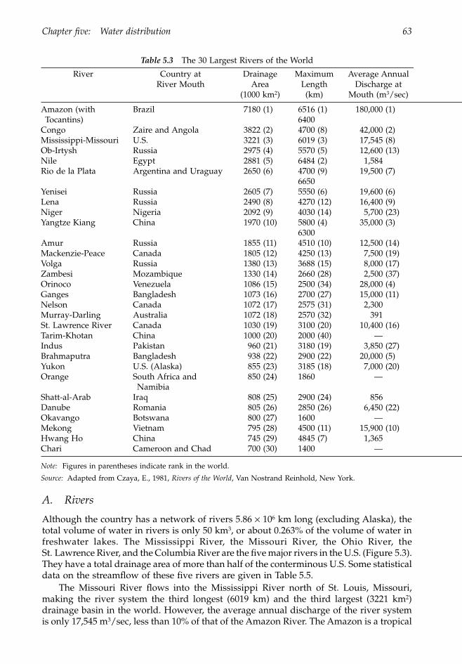
Chapter five: Water distribution 63
A. Rivers
Although the country has a network of rivers 5.86 ¥ 106 km long (excluding Alaska), thetotal volume of water in rivers is only 50 km3, or about 0.263% of the volume of water infreshwater lakes. The Mississippi River, the Missouri River, the Ohio River, theSt. Lawrence River, and the Columbia River are the five major rivers in the U.S. (Figure 5.3).They have a total drainage area of more than half of the conterminous U.S. Some statisticaldata on the streamflow of these five rivers are given in Table 5.5.
The Missouri River flows into the Mississippi River north of St. Louis, Missouri,making the river system the third longest (6019 km) and the third largest (3221 km2)drainage basin in the world. However, the average annual discharge of the river systemis only 17,545 m3/sec, less than 10% of that of the Amazon River. The Amazon is a tropical
Table 5.3 The 30 Largest Rivers of the World
River Country at River Mouth
Drainage Area
(1000 km2)
Maximum Length
(km)
Average Annual Discharge at
Mouth (m3/sec)
Amazon (with Tocantins)
Brazil 7180 (1) 6516 (1)6400
180,000 (1)
Congo Zaire and Angola 3822 (2) 4700 (8) 42,000 (2)Mississippi-Missouri U.S. 3221 (3) 6019 (3) 17,545 (8) Ob-Irtysh Russia 2975 (4) 5570 (5) 12,600 (13)Nile Egypt 2881 (5) 6484 (2) 1,584 Rio de la Plata Argentina and Uraguay 2650 (6) 4700 (9)
665019,500 (7)
Yenisei Russia 2605 (7) 5550 (6) 19,600 (6)Lena Russia 2490 (8) 4270 (12) 16,400 (9)Niger Nigeria 2092 (9) 4030 (14) 5,700 (23)Yangtze Kiang China 1970 (10) 5800 (4)
630035,000 (3)
Amur Russia 1855 (11) 4510 (10) 12,500 (14)Mackenzie-Peace Canada 1805 (12) 4250 (13) 7,500 (19)Volga Russia 1380 (13) 3688 (15) 8,000 (17)Zambesi Mozambique 1330 (14) 2660 (28) 2,500 (37)Orinoco Venezuela 1086 (15) 2500 (34) 28,000 (4)Ganges Bangladesh 1073 (16) 2700 (27) 15,000 (11)Nelson Canada 1072 (17) 2575 (31) 2,300Murray-Darling Australia 1072 (18) 2570 (32) 391St. Lawrence River Canada 1030 (19) 3100 (20) 10,400 (16)Tarim-Khotan China 1000 (20) 2000 (40) —Indus Pakistan 960 (21) 3180 (19) 3,850 (27)Brahmaputra Bangladesh 938 (22) 2900 (22) 20,000 (5)Yukon U.S. (Alaska) 855 (23) 3185 (18) 7,000 (20)Orange South Africa and
Namibia850 (24) 1860 —
Shatt-al-Arab Iraq 808 (25) 2900 (24) 856Danube Romania 805 (26) 2850 (26) 6,450 (22)Okavango Botswana 800 (27) 1600 —Mekong Vietnam 795 (28) 4500 (11) 15,900 (10)Hwang Ho China 745 (29) 4845 (7) 1,365 Chari Cameroon and Chad 700 (30) 1400 —
Note: Figures in parentheses indicate rank in the world.
Source: Adapted from Czaya, E., 1981, Rivers of the World, Van Nostrand Reinhold, New York.
1363_C05_fm Page 63 Wednesday, December 4, 2002 7:40 AM
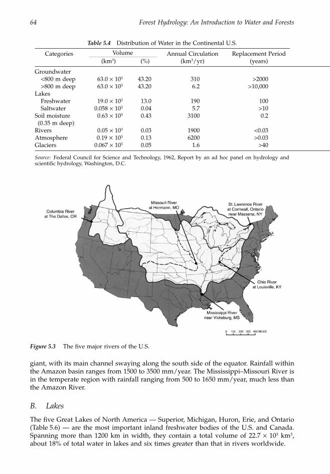
64 Forest Hydrology: An Introduction to Water and Forests
giant, with its main channel swaying along the south side of the equator. Rainfall withinthe Amazon basin ranges from 1500 to 3500 mm/year. The Mississippi–Missouri River isin the temperate region with rainfall ranging from 500 to 1650 mm/year, much less thanthe Amazon River.
B. Lakes
The five Great Lakes of North America — Superior, Michigan, Huron, Erie, and Ontario(Table 5.6) — are the most important inland freshwater bodies of the U.S. and Canada.Spanning more than 1200 km in width, they contain a total volume of 22.7 ¥ 103 km3,about 18% of total water in lakes and six times greater than that in rivers worldwide.
Table 5.4 Distribution of Water in the Continental U.S.
Categories Volume Annual Circulation Replacement Period(km3) (%) (km3/yr) (years)
Groundwater<800 m deep 63.0 ¥ 103 43.20 310 >2000>800 m deep 63.0 ¥ 103 43.20 6.2 >10,000
LakesFreshwater 19.0 ¥ 103 13.0 190 100Saltwater 0.058 ¥ 103 0.04 5.7 >10
Soil moisture(0.35 m deep)
0.63 ¥ 103 0.43 3100 0.2
Rivers 0.05 ¥ 103 0.03 1900 <0.03Atmosphere 0.19 ¥ 103 0.13 6200 >0.03Glaciers 0.067 ¥ 103 0.05 1.6 >40
Source: Federal Council for Science and Technology, 1962, Report by an ad hoc panel on hydrology andscientific hydrology, Washington, D.C.
Figure 5.3 The five major rivers of the U.S.
1363_C05_fm Page 64 Wednesday, December 4, 2002 7:40 AM
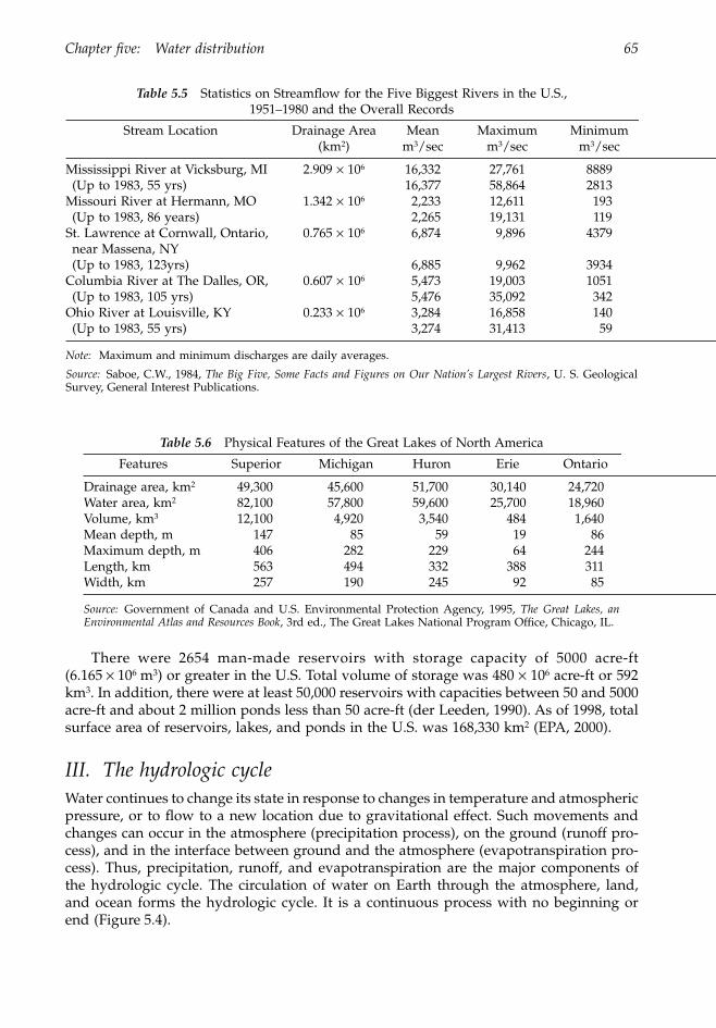
Chapter five: Water distribution 65
There were 2654 man-made reservoirs with storage capacity of 5000 acre-ft(6.165 ¥ 106 m3) or greater in the U.S. Total volume of storage was 480 ¥ 106 acre-ft or 592km3. In addition, there were at least 50,000 reservoirs with capacities between 50 and 5000acre-ft and about 2 million ponds less than 50 acre-ft (der Leeden, 1990). As of 1998, totalsurface area of reservoirs, lakes, and ponds in the U.S. was 168,330 km2 (EPA, 2000).
III. The hydrologic cycleWater continues to change its state in response to changes in temperature and atmosphericpressure, or to flow to a new location due to gravitational effect. Such movements andchanges can occur in the atmosphere (precipitation process), on the ground (runoff pro-cess), and in the interface between ground and the atmosphere (evapotranspiration pro-cess). Thus, precipitation, runoff, and evapotranspiration are the major components ofthe hydrologic cycle. The circulation of water on Earth through the atmosphere, land,and ocean forms the hydrologic cycle. It is a continuous process with no beginning orend (Figure 5.4).
Table 5.5 Statistics on Streamflow for the Five Biggest Rivers in the U.S., 1951–1980 and the Overall Records
Stream Location Drainage Area (km2)
Mean m3/sec
Maximum m3/sec
Minimum m3/sec
Mississippi River at Vicksburg, MI 2.909 ¥ 106 16,332 27,761 8889(Up to 1983, 55 yrs) 16,377 58,864 2813
Missouri River at Hermann, MO 1.342 ¥ 106 2,233 12,611 193(Up to 1983, 86 years) 2,265 19,131 119
St. Lawrence at Cornwall, Ontario, near Massena, NY
0.765 ¥ 106 6,874 9,896 4379
(Up to 1983, 123yrs) 6,885 9,962 3934Columbia River at The Dalles, OR, 0.607 ¥ 106 5,473 19,003 1051(Up to 1983, 105 yrs) 5,476 35,092 342
Ohio River at Louisville, KY 0.233 ¥ 106 3,284 16,858 140(Up to 1983, 55 yrs) 3,274 31,413 59
Note: Maximum and minimum discharges are daily averages.
Source: Saboe, C.W., 1984, The Big Five, Some Facts and Figures on Our Nation’s Largest Rivers, U. S. GeologicalSurvey, General Interest Publications.
Table 5.6 Physical Features of the Great Lakes of North America
Features Superior Michigan Huron Erie Ontario
Drainage area, km2 49,300 45,600 51,700 30,140 24,720Water area, km2 82,100 57,800 59,600 25,700 18,960Volume, km3 12,100 4,920 3,540 484 1,640Mean depth, m 147 85 59 19 86Maximum depth, m 406 282 229 64 244Length, km 563 494 332 388 311Width, km 257 190 245 92 85
Source: Government of Canada and U.S. Environmental Protection Agency, 1995, The Great Lakes, anEnvironmental Atlas and Resources Book, 3rd ed., The Great Lakes National Program Office, Chicago, IL.
1363_C05_fm Page 65 Wednesday, December 4, 2002 7:40 AM
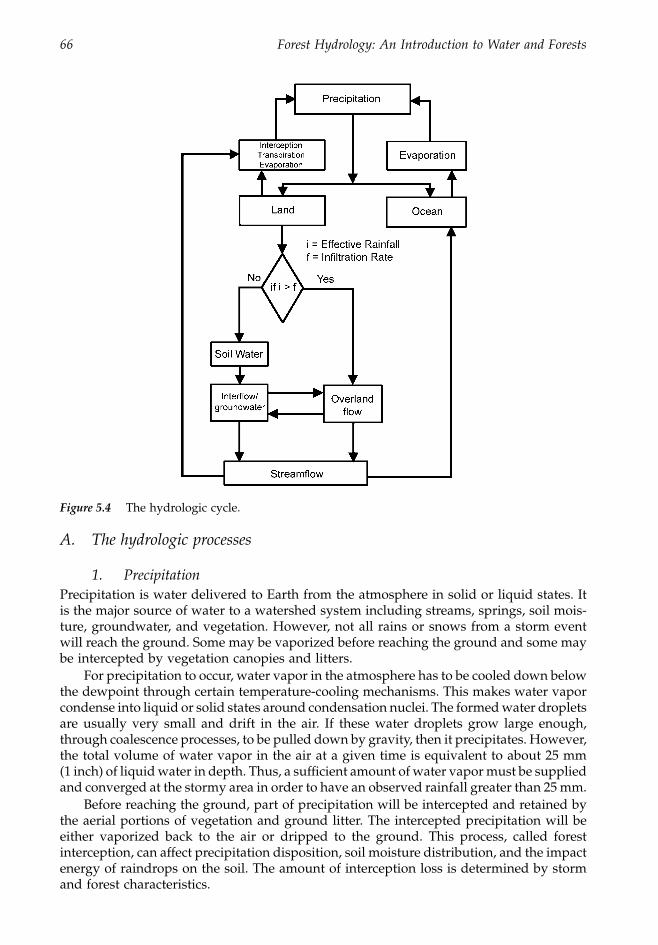
66 Forest Hydrology: An Introduction to Water and Forests
A. The hydrologic processes
1. PrecipitationPrecipitation is water delivered to Earth from the atmosphere in solid or liquid states. Itis the major source of water to a watershed system including streams, springs, soil mois-ture, groundwater, and vegetation. However, not all rains or snows from a storm eventwill reach the ground. Some may be vaporized before reaching the ground and some maybe intercepted by vegetation canopies and litters.
For precipitation to occur, water vapor in the atmosphere has to be cooled down belowthe dewpoint through certain temperature-cooling mechanisms. This makes water vaporcondense into liquid or solid states around condensation nuclei. The formed water dropletsare usually very small and drift in the air. If these water droplets grow large enough,through coalescence processes, to be pulled down by gravity, then it precipitates. However,the total volume of water vapor in the air at a given time is equivalent to about 25 mm(1 inch) of liquid water in depth. Thus, a sufficient amount of water vapor must be suppliedand converged at the stormy area in order to have an observed rainfall greater than 25 mm.
Before reaching the ground, part of precipitation will be intercepted and retained bythe aerial portions of vegetation and ground litter. The intercepted precipitation will beeither vaporized back to the air or dripped to the ground. This process, called forestinterception, can affect precipitation disposition, soil moisture distribution, and the impactenergy of raindrops on the soil. The amount of interception loss is determined by stormand forest characteristics.
Figure 5.4 The hydrologic cycle.
1363_C05_fm Page 66 Wednesday, December 4, 2002 7:40 AM
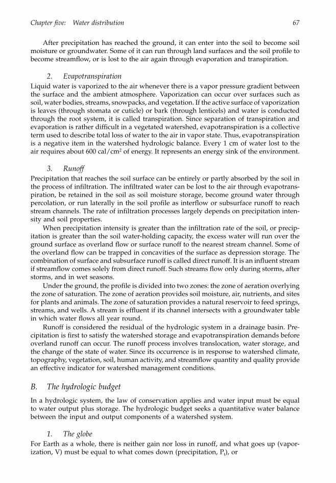
Chapter five: Water distribution 67
After precipitation has reached the ground, it can enter into the soil to become soilmoisture or groundwater. Some of it can run through land surfaces and the soil profile tobecome streamflow, or is lost to the air again through evaporation and transpiration.
2. EvapotranspirationLiquid water is vaporized to the air whenever there is a vapor pressure gradient betweenthe surface and the ambient atmosphere. Vaporization can occur over surfaces such assoil, water bodies, streams, snowpacks, and vegetation. If the active surface of vaporizationis leaves (through stomata or cuticle) or bark (through lenticels) and water is conductedthrough the root system, it is called transpiration. Since separation of transpiration andevaporation is rather difficult in a vegetated watershed, evapotranspiration is a collectiveterm used to describe total loss of water to the air in vapor state. Thus, evapotranspirationis a negative item in the watershed hydrologic balance. Every 1 cm of water lost to theair requires about 600 cal/cm2 of energy. It represents an energy sink of the environment.
3. RunoffPrecipitation that reaches the soil surface can be entirely or partly absorbed by the soil inthe process of infiltration. The infiltrated water can be lost to the air through evapotrans-piration, be retained in the soil as soil moisture storage, become ground water throughpercolation, or run laterally in the soil profile as interflow or subsurface runoff to reachstream channels. The rate of infiltration processes largely depends on precipitation inten-sity and soil properties.
When precipitation intensity is greater than the infiltration rate of the soil, or precip-itation is greater than the soil water-holding capacity, the excess water will run over theground surface as overland flow or surface runoff to the nearest stream channel. Some ofthe overland flow can be trapped in concavities of the surface as depression storage. Thecombination of surface and subsurface runoff is called direct runoff. It is an influent streamif streamflow comes solely from direct runoff. Such streams flow only during storms, afterstorms, and in wet seasons.
Under the ground, the profile is divided into two zones: the zone of aeration overlyingthe zone of saturation. The zone of aeration provides soil moisture, air, nutrients, and sitesfor plants and animals. The zone of saturation provides a natural reservoir to feed springs,streams, and wells. A stream is effluent if its channel intersects with a groundwater tablein which water flows all year round.
Runoff is considered the residual of the hydrologic system in a drainage basin. Pre-cipitation is first to satisfy the watershed storage and evapotranspiration demands beforeoverland runoff can occur. The runoff process involves translocation, water storage, andthe change of the state of water. Since its occurrence is in response to watershed climate,topography, vegetation, soil, human activity, and streamflow quantity and quality providean effective indicator for watershed management conditions.
B. The hydrologic budget
In a hydrologic system, the law of conservation applies and water input must be equalto water output plus storage. The hydrologic budget seeks a quantitative water balancebetween the input and output components of a watershed system.
1. The globeFor Earth as a whole, there is neither gain nor loss in runoff, and what goes up (vapor-ization, V) must be equal to what comes down (precipitation, Pt), or
1363_C05_fm Page 67 Wednesday, December 4, 2002 7:40 AM
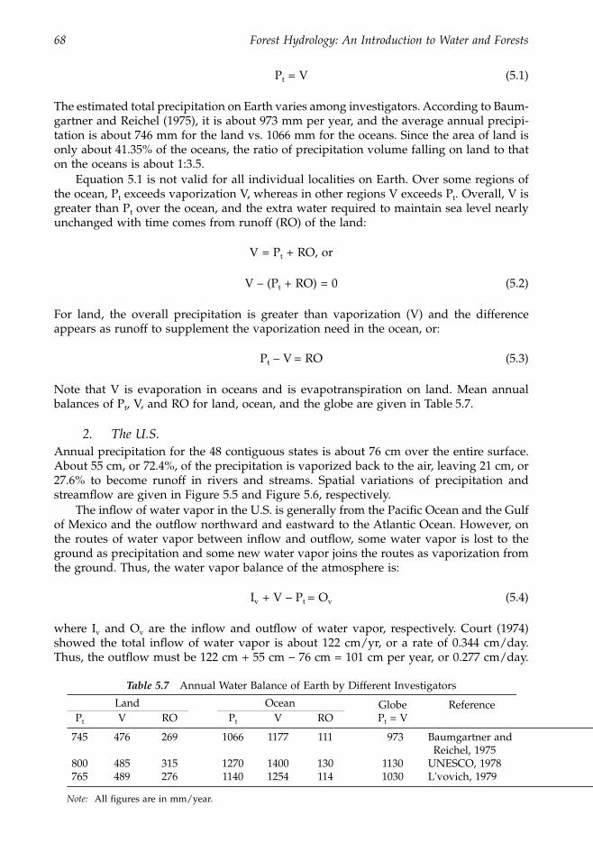
68 Forest Hydrology: An Introduction to Water and Forests
Pt = V (5.1)
The estimated total precipitation on Earth varies among investigators. According to Baum-gartner and Reichel (1975), it is about 973 mm per year, and the average annual precipi-tation is about 746 mm for the land vs. 1066 mm for the oceans. Since the area of land isonly about 41.35% of the oceans, the ratio of precipitation volume falling on land to thaton the oceans is about 1:3.5.
Equation 5.1 is not valid for all individual localities on Earth. Over some regions ofthe ocean, Pt exceeds vaporization V, whereas in other regions V exceeds Pt. Overall, V isgreater than Pt over the ocean, and the extra water required to maintain sea level nearlyunchanged with time comes from runoff (RO) of the land:
V = Pt + RO, or
V – (Pt + RO) = 0 (5.2)
For land, the overall precipitation is greater than vaporization (V) and the differenceappears as runoff to supplement the vaporization need in the ocean, or:
Pt – V = RO (5.3)
Note that V is evaporation in oceans and is evapotranspiration on land. Mean annualbalances of Pt, V, and RO for land, ocean, and the globe are given in Table 5.7.
2. The U.S.Annual precipitation for the 48 contiguous states is about 76 cm over the entire surface.About 55 cm, or 72.4%, of the precipitation is vaporized back to the air, leaving 21 cm, or27.6% to become runoff in rivers and streams. Spatial variations of precipitation andstreamflow are given in Figure 5.5 and Figure 5.6, respectively.
The inflow of water vapor in the U.S. is generally from the Pacific Ocean and the Gulfof Mexico and the outflow northward and eastward to the Atlantic Ocean. However, onthe routes of water vapor between inflow and outflow, some water vapor is lost to theground as precipitation and some new water vapor joins the routes as vaporization fromthe ground. Thus, the water vapor balance of the atmosphere is:
Iv + V – Pt = Ov (5.4)
where Iv and Ov are the inflow and outflow of water vapor, respectively. Court (1974)showed the total inflow of water vapor is about 122 cm/yr, or a rate of 0.344 cm/day.Thus, the outflow must be 122 cm + 55 cm - 76 cm = 101 cm per year, or 0.277 cm/day.
Table 5.7 Annual Water Balance of Earth by Different Investigators
Land Ocean Globe ReferencePt V RO Pt V RO Pt = V
745 476 269 1066 1177 111 973 Baumgartner and Reichel, 1975
800 485 315 1270 1400 130 1130 UNESCO, 1978765 489 276 1140 1254 114 1030 L'vovich, 1979
Note: All figures are in mm/year.
1363_C05_fm Page 68 Wednesday, December 4, 2002 7:40 AM
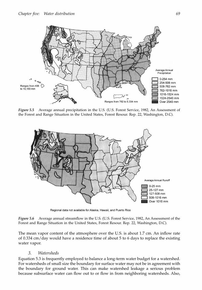
Chapter five: Water distribution 69
The mean vapor content of the atmosphere over the U.S. is about 1.7 cm. An inflow rateof 0.334 cm/day would have a residence time of about 5 to 6 days to replace the existingwater vapor.
3. WatershedsEquation 5.3 is frequently employed to balance a long-term water budget for a watershed.For watersheds of small size the boundary for surface water may not be in agreement withthe boundary for ground water. This can make watershed leakage a serious problembecause subsurface water can flow out to or flow in from neighboring watersheds. Also,
Figure 5.5 Average annual precipitation in the U.S. (U.S. Forest Service, 1982, An Assessment ofthe Forest and Range Situation in the United States, Forest Resour. Rep. 22, Washington, D.C).
Figure 5.6 Average annual streamflow in the U.S. (U.S. Forest Service, 1982, An Assessment of theForest and Range Situation in the United States, Forest Resour. Rep. 22, Washington, D.C).
1363_C05_fm Page 69 Wednesday, December 4, 2002 7:40 AM
70 Forest Hydrology: An Introduction to Water and Forests
small watersheds may have unsteady soil moisture storage, especially during short periodsof time. Under these circumstances, watershed hydrologic balance should take this form:
Pt – RO - V + DS + DL = 0 (5.5)
where DS and DL are, respectively, changes in soil moisture storage and watershed leakage.Note that the variables DS or DL can be positive or negative. If gauging stations arecarefully constructed with no occurrence of seepage, such as in many experimental water-sheds, and there is no subsurface inflow and outflow caused by physiographic features,DL = 0 and Equation 5.5 can be employed to solve for vaporization loss V.
Since there is so much variation in the geology, soil, topography, vegetation, andclimate within a watershed, many hydrologic studies have been conducted on small plotsthat are more uniform in environmental conditions. The small plot watershed approachmakes replication of treatments possible. During a dry period, Pt = 0, no free water isstanding in the soil profile of small plot watersheds. Thus it is logical to assume that thereis no surface runoff, no downward water percolation, and no lateral movement of sub-surface water in or out of the plot. In this case Equation 5.5 becomes:
V = DS (5.6)
or changes in soil moisture storage can be used to estimate V of the plot. If the soil surfaceis sealed to prevent soil evaporation, then DS is a measure of plant transpiration.
C. The energy budget
The hydrological cycle described above is a continuous change of the state of waterbetween Earth and the atmosphere. A tremendous amount of energy is involved in everycomponent and process of this cycle. Without this supply of energy, there would be nohydrologic cycle and no climate changes.
The major components that affect net radiation (Rn) of a location are incoming solarradiation (Rs), outgoing solar reflection (Rr), incoming atmospheric radiation (Ra), andoutgoing terrestrial radiation (Rg). In equation form, it appears:
Rn = Rs – Rr+ Ra – Rg (5.7)
Net radiation can be negative, depending on geographic location, season of the year, timeof day, and duration. The observed net radiation is further dissipated into latent heat (Lh),sensible heat (Sh), and conductive heat (Ch), or:
Rn = Lh + Sh + Ch (5.8)
For long-term averages, Ch is considered constant, then Rn is dissipated into either Lh or Sh.Table 5.8 shows the average net radiation to be 49 kcal cm-2 yr-1 for land, 91 kcal cm–2 yr–1
for ocean, and 79 kcal cm-2 yr-1 for Earth as a whole. Of the total net radiation of Earth,about 67 kcal cm-2 yr-1 or 84.5% is used for vaporization. Average temperature of Earthis about 300∞K. The latent heat of vaporization corresponding to the 300∞K is 582 cal forevery cm3 of water. In other words, the 67 kcal cm-2 yr-1 of Lh is sufficient to vaporizeabout 1151 mm of water every year (see Table 5.7).
The heat budgets of different continents and oceans are given in Table 5.9. In humidareas where water is not a limiting factor for vaporization, Lh takes a greater proportionthan Sh does. On the other hand, in arid areas such as land at 20 to 30∞ north and southlatitudes, water shortage causes Sh to use a greater proportion of Rn than does Lh (Table 5.8).
1363_C05_fm Page 70 Wednesday, December 4, 2002 7:40 AM
Chapter five: Water distribution 71
Tabl
e 5.
8H
eat
Bal
ance
, in
kcal
cm
---- 2/
year
---- 1, o
f E
arth
's S
urfa
ce a
nd o
f th
e A
tmos
pher
e
Lat
itud
eL
and
Oce
anE
arth
as
a w
hole
Atm
osph
ere
Rn
Lh
S hR
nL
hS h
F oR
nL
hS h
F oR
aL
r
70–6
0 N
2016
422
2623
-27
2119
10-8
-77
3460
–50
3023
740
4719
-26
3433
12-1
1-6
651
50–4
045
2520
6365
15-1
754
4418
-8-6
651
40–3
060
2337
9096
15-2
177
6524
-12
-76
4630
–20
6919
5011
110
67
-29 5
7 32 3
-1-9
039
20–1
071
3239
123
117
7-1
109
9415
0-9
170
10–0
072
5715
126
106
713
114
959
10-8
412
800
–10
S72
6111
128
976
2511
588
720
-81
101
10–2
073
4528
123
113
91
115
9813
0-8
474
20–3
070
2842
110
108
11-9
101
9018
-7-8
161
30–4
062
2933
9386
11-4
8 97 9
1 4-4
-78
6840
–50
4122
1972
384
2071
474
20-7
077
50–6
031
229
4534
92
4534
92
-63
89O
vera
ll49
2722
9182
90
7967
120
-79
67
Not
e:
Rn =
net
rad
iati
on b
alan
ce a
t Ear
th's
sur
face
; Lh =
late
nt h
eat;
S h =
sen
sibl
e he
at; F
o = re
dis
trib
utio
n of
hea
t by
sea
curr
ents
; Ra =
rad
iati
on b
alan
ce o
f the
atm
osph
ere;
Lr =
hea
t in
put
from
con
den
sati
on in
the
atm
osph
ere.
The
qua
ntit
ies
Rn,
Ra,
and
Lr a
re t
aken
as
posi
tive
whe
n th
ey r
epre
sent
a h
eat
inpu
t, an
d o
ther
qua
ntit
ies
as p
osit
ive
whe
n th
ey r
epre
sent
an
expe
ndit
ure
of h
eat.
Sour
ce:
UN
ESC
O, 1
978,
Wor
ld W
ater
Bal
ance
and
Wat
er R
esou
rces
of t
he E
arth
, UN
ESC
O P
ress
, Par
is. W
ith
perm
issi
on.
1363_C05_fm Page 71 Wednesday, December 4, 2002 7:40 AM
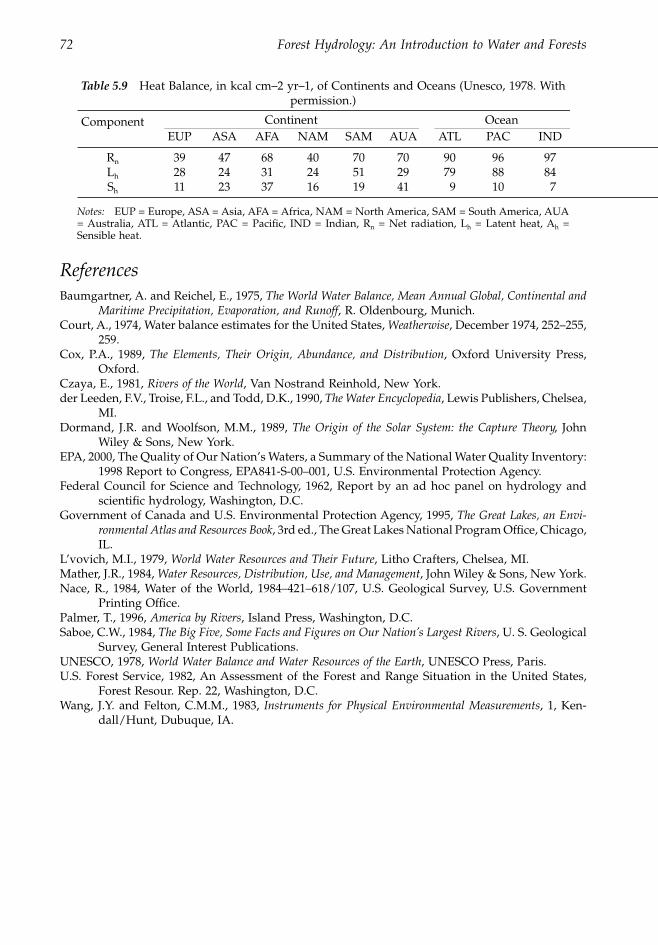
72 Forest Hydrology: An Introduction to Water and Forests
ReferencesBaumgartner, A. and Reichel, E., 1975, The World Water Balance, Mean Annual Global, Continental and
Maritime Precipitation, Evaporation, and Runoff, R. Oldenbourg, Munich.Court, A., 1974, Water balance estimates for the United States, Weatherwise, December 1974, 252–255,
259.Cox, P.A., 1989, The Elements, Their Origin, Abundance, and Distribution, Oxford University Press,
Oxford.Czaya, E., 1981, Rivers of the World, Van Nostrand Reinhold, New York.der Leeden, F.V., Troise, F.L., and Todd, D.K., 1990, The Water Encyclopedia, Lewis Publishers, Chelsea,
MI.Dormand, J.R. and Woolfson, M.M., 1989, The Origin of the Solar System: the Capture Theory, John
Wiley & Sons, New York.EPA, 2000, The Quality of Our Nation’s Waters, a Summary of the National Water Quality Inventory:
1998 Report to Congress, EPA841-S-00–001, U.S. Environmental Protection Agency.Federal Council for Science and Technology, 1962, Report by an ad hoc panel on hydrology and
scientific hydrology, Washington, D.C.Government of Canada and U.S. Environmental Protection Agency, 1995, The Great Lakes, an Envi-
ronmental Atlas and Resources Book, 3rd ed., The Great Lakes National Program Office, Chicago,IL.
L’vovich, M.I., 1979, World Water Resources and Their Future, Litho Crafters, Chelsea, MI.Mather, J.R., 1984, Water Resources, Distribution, Use, and Management, John Wiley & Sons, New York.Nace, R., 1984, Water of the World, 1984–421–618/107, U.S. Geological Survey, U.S. Government
Printing Office.Palmer, T., 1996, America by Rivers, Island Press, Washington, D.C.Saboe, C.W., 1984, The Big Five, Some Facts and Figures on Our Nation’s Largest Rivers, U. S. Geological
Survey, General Interest Publications.UNESCO, 1978, World Water Balance and Water Resources of the Earth, UNESCO Press, Paris.U.S. Forest Service, 1982, An Assessment of the Forest and Range Situation in the United States,
Forest Resour. Rep. 22, Washington, D.C.Wang, J.Y. and Felton, C.M.M., 1983, Instruments for Physical Environmental Measurements, 1, Ken-
dall/Hunt, Dubuque, IA.
Table 5.9 Heat Balance, in kcal cm–2 yr–1, of Continents and Oceans (Unesco, 1978. With permission.)
Component Continent OceanEUP ASA AFA NAM SAM AUA ATL PAC IND
Rn 39 47 68 40 70 70 90 96 97Lh 28 24 31 24 51 29 79 88 84Sh 11 23 37 16 19 41 9 10 7
Notes: EUP = Europe, ASA = Asia, AFA = Africa, NAM = North America, SAM = South America, AUA= Australia, ATL = Atlantic, PAC = Pacific, IND = Indian, Rn = Net radiation, Lh = Latent heat, Ah =Sensible heat.
1363_C05_fm Page 72 Wednesday, December 4, 2002 7:40 AM
73
chapter six
Water resource problems
Contents
I. Water demand and supply ..............................................................................................75A. Water demand ...........................................................................................................75
1. The world.............................................................................................................752. The U.S. ................................................................................................................753. Projections for the U.S. ......................................................................................76
B. Water supply..............................................................................................................781. The world.............................................................................................................782. The U.S. ................................................................................................................80
II. Water quantity ...................................................................................................................82A. Drought ......................................................................................................................82
1. Rainmaking..........................................................................................................832. Water translocation.............................................................................................833. Desalination .........................................................................................................844. Water reclamation...............................................................................................845. Rain harvesting ...................................................................................................856. Iceberg harvesting...............................................................................................867. Household conservation....................................................................................868. Evaporation reduction .......................................................................................869. Irrigation efficiency.............................................................................................8710. Vegetation control ...............................................................................................8711. Genetic engineering............................................................................................8812. Drought forecast .................................................................................................8813. Price control .........................................................................................................88
B. Floods..........................................................................................................................891. Forms and causes................................................................................................89
a. Flash flood......................................................................................................89b. River flood .....................................................................................................89c. Urban flood....................................................................................................90d. Coastal flood..................................................................................................90
2. Nature of floods ..................................................................................................913. Flood damages ....................................................................................................91
a. Flood damages increase with time ............................................................92b. Losses per unit area decrease with increasing watershed size.............92c. Forested watersheds are less damaging ...................................................92d. Inundation can be a blessing ......................................................................93
1363_C06_fm Page 73 Wednesday, December 4, 2002 7:41 AM

74 Forest Hydrology: An Introduction to Water and Forests
4. Flood control and management .......................................................................93a. Flood-control measures................................................................................93b. Flood forecasting...........................................................................................95c. Floodplain zoning.........................................................................................95d. Flood insurance.............................................................................................96e. Disaster aids...................................................................................................97
III. Water quality......................................................................................................................97A. Water pollutants........................................................................................................98
1. Sediments .............................................................................................................982. Heat .......................................................................................................................983. Oxygen-demanding wastes...............................................................................994. Plant nutrients .....................................................................................................995. Disease-causing agents ......................................................................................996. Inorganic chemicals and minerals .................................................................1007. Synthetic organic chemicals ............................................................................1008. Radioactive substances ....................................................................................100
B. Sources of water pollution ....................................................................................100C. Water quality control..............................................................................................101
1. Monitoring and research .................................................................................1022. Public education................................................................................................1023. Prevention and treatment................................................................................1024. Management ......................................................................................................1025. Legislation and enforcement...........................................................................103
D. Water-quality laws and regulations.....................................................................103IV. Water rights ......................................................................................................................103
A. Diffused water.........................................................................................................104B. Surface water ...........................................................................................................104
1. Riparian rights.............................................................................................1042 Prior appropriation.....................................................................................1053 Hybrid doctrine...........................................................................................1054. Reserved-rights doctrine............................................................................105
C. Groundwater ...........................................................................................................106References .....................................................................................................................................106
Water resource problems are problems of water quantity, quality, and timing. Some regionsmay have too much water (flooding), while others may have too little water (drought).Water may not occur at the right time and in the right place (timing), or water may notbe clean enough for drinking and other uses (water pollution). Moreover, the complexityof water usage in our modern society and the requirement of water for economic devel-opment make the rights to capture water and water allocation important issues in waterresources (water rights). No region in the world is immune from these problems, whichstem from the uneven distribution of water, water mobility, imbalance in supply anddemand, steady increases in population, economic growth, poor environmental manage-ment, and lack of concern by the public.
1363_C06_fm Page 74 Wednesday, December 4, 2002 7:41 AM

Chapter six: Water resource problems 75
I. Water demand and supply
A. Water demand
Water demand is often described as either water withdrawal or water consumption. Theterm withdrawal refers to pumping or taking water from a source for various uses orstorage. Water consumption or consumptive use of water refers to the part of withdrawnwater that is vaporized to the air, consumed by humans, plants or livestock, incorporatedinto products, and not discharged into a supply source for potential reuse.
1. The world
Total freshwater consumption of the world increased from 1.589 km
3
/d in 1900 to about3.699 km
3
/d in 1950 and 11.342 km
3
/d in 1990 (Jordaan et al., 1993; Gleick, 1998). Theconsumption rate increased about 0.042 km
3
/d/year (15.403 km
3
/year) between 1900 and1950, and about 0.191 km
3
/d/year (69.742 km
3
/year) between 1950 and 1990. In otherwords, total freshwater withdrawals increased about 7.14 times in the 90-year period(Table 6.1).
The increases in water consumption are reflections of population growth, agriculturalexpansion, and industrial development, and were most rapid after World War II. Theworld population increased 3.31 times during the 90-year period, from about 1.6 billionin 1900 and 2.5 billion in 1950 to 5.3 billion in 1990. Total water withdrawals on a percapita basis were 0.993 m
3
/person/d in 1900 and doubled to 2.140 m
3
/person/d in 1990.Agriculture is the biggest consumer despite a continuing fall in its proportion of total
water consumption from 90.5% (525 km
3
/year) in 1900 to 66.3% (2200 km
3
/year) in 1980and to an expected 62.6% (3250 km
3
/year) in 2000. During the same period, industry used6.4% in 1900, 18.8% in 1980, and an expected 24.7% in 2000 (Figure 6.1). Of the majorregions around the world, Asia and Oceania, the biggest water consumers and the fastestgrowing regions in the world, made up 60% of the world’s total consumption in 1990(Table 6.1). Because of abundant water resources, both the volume and growth rate ofwater consumption are the smallest in South America (WMO/UNESCO, 1991).
2. The U.S.
The rates of total withdrawals in the U.S. were much greater than the average withdrawalrate of the world. In 1900, The U.S. population was 76 million or only 4.75% of the world.Total withdrawals, however, were 0.153 km
3
/day, or almost 10% of the world. This wasa per capita withdrawal of 2.019 m
3
/person/d, about double that of the world average.Interesting enough, 90 years later the U.S. population maintained at 4.75% (252 million)of the world total, but total withdrawals increased to 1.545 km
3
/d (Solley et al., 1998), or
Table 6.1
Trends in World Water Consumption (in km
3
/year) by Region
Region 1900 1940 1950 1960 1970 1980 1990 2000
Africa 41.8 49.2 56.2 86.2 116.0 168.0 232.0 317.0Europe 37.5 70.9 93.8 105.0 294.0 435.0 554.0 673.0North and South America
84.5 249.0 345.0 475.0 641.0 774.0 874.0 1012.0
Asia and Oceania
416.0 689.0 869.0 1237.0 1543.0 1940.0 2480.0 3190.0
World 580.0 1060.0 1350.0 1980.0 2590.0 3320.0 4140.0 5190.0Population, 10
9
1.6 2.3 2.5 3.0 3.7 4.5 5.3 6.3
Source:
UNESCO, 1993,
Water for the Common Future
, International Hydro. Prog., Committee on Water Res., Paris.
1363_C06_fm Page 75 Wednesday, December 4, 2002 7:41 AM
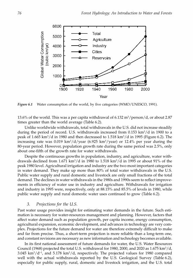
76 Forest Hydrology: An Introduction to Water and Forests
13.6% of the world. This was a per capita withdrawal of 6.132 m
3
/person/d, or about 2.87times greater than the world average (Table 6.2).
Unlike worldwide withdrawals, total withdrawals in the U.S. did not increase steadilyduring the period of record. U.S. withdrawals increased from 0.153 km
3
/d in 1900 to apeak of 1.665 km
3
/d in 1980 and then decreased to 1.518 km
3
/d in 1995 (Figure 6.2). Theincreasing rate was 0.019 km
3
/d/year (6.925 km
3
/year) or 12.4% per year during the80-year period. However, population growth rate during the same period was 2.5%, onlyabout one-fifth of the growth rate for water withdrawals.
Despite the continuous growths in population, industry, and agriculture, water with-drawals declined from 1.671 km
3
/d in 1980 to 1.518 km
3
/d in 1995 or about 91% of thepeak 1980 level. Agricultural irrigation and industry are the two most important categoriesin water demand. They make up more than 80% of total water withdrawals in the U.S.Public water supply and rural domestic and livestock are only small fractions of the totaldemand. The declines in water withdrawals in the 1980s and 1990s seem to reflect improve-ments in efficiency of water use in industry and agriculture. Withdrawals for irrigationand industry in 1995 were, respectively, only at 88.15% and 85.5% of levels in 1980, whilepublic water supply and rural domestic water uses continued to grow (Table 6.2).
3. Projections for the U.S.
Past water usage provides insight for estimating water demands in the future. Such esti-mation is necessary for water-resources management and planning. However, factors thataffect water demand such as population growth, per capita income, energy consumption,agricultural expansion, economic development, and advances in technology are very com-plex. Projections for the future demand for water are therefore extremely difficult to makeand far from precise. Thus, a short-term projection is more reliable than a long-term one,and constant revisions are necessary as new information and technology becomes available.
In its first national assessment of future demands for water, the U.S. Water ResourcesCouncil (1968) projected the total U.S. withdrawal for 1980, 2000, and 2020 as 1.675 km
3
/d,3.045 km
3
/d
-
1
, and 5.178 km
3
/d, respectively. The projected values for 1980 comparedwell with the actual withdrawals reported by the U.S. Geological Survey (Table 6.2),especially for public supply, rural, domestic and livestock irrigation, and the U.S. total
Figure 6.1
Water consumption of the world, by five categories (WMO/UNESCO, 1991).
1363_C06_fm Page 76 Wednesday, December 4, 2002 7:41 AM
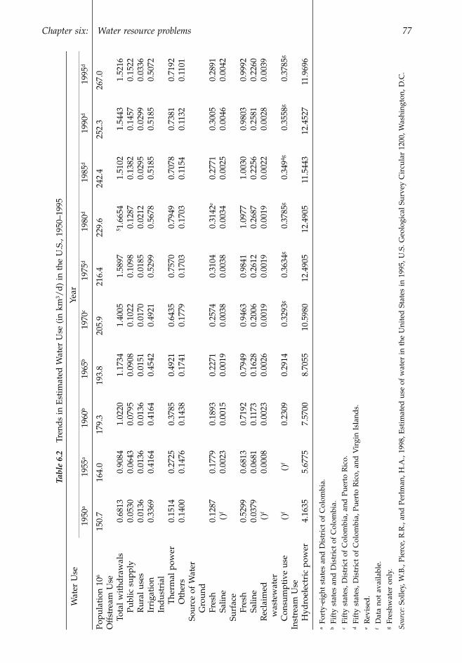
Chapter six: Water resource problems 77
Tabl
e 6.
2
Tren
ds
in E
stim
ated
Wat
er U
se (
in k
m
3
/d
) in
the
U.S
., 19
50–1
995
Wat
er U
se
Year
1950
a
1955
a
1960
b
1965
b
1970
c
1975
d
1980
d
1985
d
1990
d
1995
d
Popu
lati
on 1
0
6
150.
716
4.0
179.
319
3.8
205.
921
6.4
229.
624
2.4
252.
326
7.0
Off
stre
am U
seTo
tal w
ithd
raw
als
0.68
130.
9084
1.02
201.
1734
1.40
051.
5897
5
1.66
541.
5102
1.54
431.
5216
Publ
ic s
uppl
y0.
0530
0.06
430.
0795
0.09
080.
1022
0.10
980.
1287
0.13
820.
1457
0.15
22R
ural
use
s0.
0136
0.01
360.
0136
0.01
510.
0170
0.01
850.
0212
0.02
950.
0299
0.03
36Ir
riga
tion
0.33
690.
4164
0.41
640.
4542
0.49
210.
5299
0.56
780.
5185
0.51
850.
5072
Ind
ustr
ial
The
rmal
pow
er
0.15
140.
2725
0.37
850.
4921
0.64
350.
7570
0.79
490.
7078
0.73
810.
7192
Oth
ers
0.14
000.
1476
0.14
380.
1741
0.17
790.
1703
0.17
030.
1154
0.11
320.
1101
Sour
ce o
f W
ater
Gro
und
Fres
h0.
1287
0.17
790.
1893
0.22
710.
2574
0.31
040.
3142
e
0.27
710.
3005
0.28
91Sa
line
()
f
0.00
230.
0015
0.00
190.
0038
0.00
380.
0034
0.00
250.
0046
0.00
42Su
rfac
eFr
esh
0.52
990.
6813
0.71
920.
7949
0.94
630.
9841
1.09
771.
0030
0.98
030.
9992
Salin
e0.
0379
0.06
810.
1173
0.16
280.
2006
0.26
120.
2687
0.22
560.
2581
0.22
60R
ecla
imed
w
aste
wat
er()
f
0.00
080.
0023
0.00
260.
0019
0.00
190.
0019
0.00
220.
0028
0.00
39
Con
sum
ptiv
e us
e()
f
()
f
0.23
090.
2914
0.32
93
g
0.36
34
g
0.37
85
g
0.34
9
4g
0.35
58
g
0.37
85
g
Inst
ream
Use
Hyd
roel
ectr
ic p
ower
4.16
355.
6775
7.57
008.
7055
10.5
980
12.4
905
12.4
905
11.5
443
12.4
527
11.9
696
a
For
ty-e
ight
sta
tes
and
Dis
tric
t of
Col
ombi
a.
b
Fif
ty s
tate
s an
d D
istr
ict
of C
olom
bia.
c
Fif
ty s
tate
s, D
istr
ict
of C
olom
bia,
and
Pue
rto
Ric
o.
d
Fif
ty s
tate
s, D
istr
ict
of C
olom
bia,
Pue
rto
Ric
o, a
nd V
irgi
n Is
land
s.
e
Rev
ised
.
f
Dat
a no
t av
aila
ble.
g
Fre
shw
ater
onl
y.
Sour
ce:
Sol
ley,
W.B
., Pi
erce
, R.R
., an
d P
erlm
an, H
.A.,
1998
, Est
imat
ed u
se o
f w
ater
in t
he U
nite
d S
tate
s in
199
5, U
.S. G
eolo
gica
l Sur
vey
Cir
cula
r 12
00, W
ashi
ngto
n, D
.C.
1363_C06_fm Page 77 Wednesday, December 4, 2002 7:41 AM
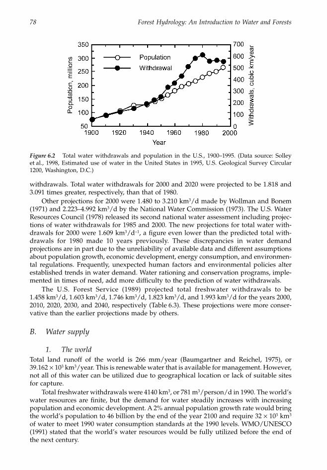
78 Forest Hydrology: An Introduction to Water and Forests
withdrawals. Total water withdrawals for 2000 and 2020 were projected to be 1.818 and3.091 times greater, respectively, than that of 1980.
Other projections for 2000 were 1.480 to 3.210 km
3
/d made by Wollman and Bonem(1971) and 2.223–4.992 km
3
/d by the National Water Commission (1973). The U.S. WaterResources Council (1978) released its second national water assessment including projec-tions of water withdrawals for 1985 and 2000. The new projections for total water with-drawals for 2000 were 1.609 km
3
/d
-
1
, a figure even lower than the predicted total with-drawals for 1980 made 10 years previously. These discrepancies in water demandprojections are in part due to the unreliability of available data and different assumptionsabout population growth, economic development, energy consumption, and environmen-tal regulations. Frequently, unexpected human factors and environmental policies alterestablished trends in water demand. Water rationing and conservation programs, imple-mented in times of need, add more difficulty to the prediction of water withdrawals.
The U.S. Forest Service (1989) projected total freshwater withdrawals to be1.458 km
3
/d, 1.603 km
3
/d, 1.746 km
3
/d, 1.823 km
3
/d, and 1.993 km
3
/d for the years 2000,2010, 2020, 2030, and 2040, respectively (Table 6.3). These projections were more conser-vative than the earlier projections made by others.
B. Water supply
1. The world
Total land runoff of the world is 266 mm/year (Baumgartner and Reichel, 1975), or39.162
¥
10
3
km
3
/year. This is renewable water that is available for management. However,not all of this water can be utilized due to geographical location or lack of suitable sitesfor capture.
Total freshwater withdrawals were 4140 km
3
, or 781 m
3
/person/d in 1990. The world’swater resources are finite, but the demand for water steadily increases with increasingpopulation and economic development. A 2% annual population growth rate would bringthe world’s population to 46 billion by the end of the year 2100 and require 32
¥
10
3
km
3
of water to meet 1990 water consumption standards at the 1990 levels. WMO/UNESCO(1991) stated that the world’s water resources would be fully utilized before the end ofthe next century.
Figure 6.2
Total water withdrawals and population in the U.S., 1900–1995. (Data source: Solleyet al., 1998, Estimated use of water in the United States in 1995, U.S. Geological Survey Circular1200, Washington, D.C.)
1363_C06_fm Page 78 Wednesday, December 4, 2002 7:41 AM
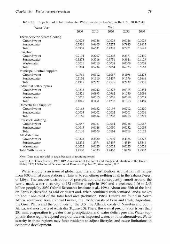
Chapter six: Water resource problems 79
Water supply is an issue of global quantity and distribution. Annual rainfall rangesfrom 4000 mm at some stations in Taiwan to sometimes nothing at all in the Sahara Desertof Libya. The uneven distribution of precipitation and consequently runoff around theworld made water a scarcity to 132 million people in 1990 and a projected 1.06 to 2.43billion people by 2050 (World Resources Institute et al., 1996). About one-fifth of the landon Earth is classified as arid or desert and, when combined with semiarid lands, makesup about one-third of the total land area (Robinson, 1988). Deserts are found in NorthAfrica, southwest Asia, Central Eurasia, the Pacific coasts of Peru and Chile, Argentina,the Great Plains and the Southwest of the U.S., the Atlantic coasts of Namibia and SouthAfrica, and most parts of Australia (Figure 6.3). There, the annual precipitation is less than254 mm, evaporation is greater than precipitation, and water deficit prevails. Water sup-plies in these regions depend on groundwater, imported water, or other alternatives. Waterscarcity in these regions may force residents to adjust lifestyles and cause limitations ineconomic development.
Table 6.3
Projection of Total Freshwater Withdrawals (in km
3
/d) in the U.S., 2000–2040
Water Use
Year2000 2010 2020 2030 2040
Thermoelectric Steam CoolingGroundwater 0.0026 0.0026 0.0026 0.0026 0.0026Surfacewater 0.5931 0.6605 0.7275 0.7945 0.8615Total 0.5958 0.6631 0.7301 0.7971 0.8641
IrrigationGroundwater 0.2104 0.2207 0.2305 0.2371 0.2430Surfacewater 0.3278 0.3516 0.3751 0.3944 0.4129Wastewater 0.0011 0.0010 0.0008 0.0008 0.0008Total 0.5394 0.5734 0.6064 0.6325 0.6563
Municipal Central SuppliesGroundwater 0.0761 0.0912 0.1067 0.1196 0.1276Surfacewater 0.1154 0.1310 0.1457 0.1576 0.1646Total 0.1915 0.2222 0.2525 0.2737 0.2918
Industrial Self-SuppliesGroundwater 0.0212 0.0242 0.0278 0.0315 0.0354Surfacewater 0.0821 0.0893 0.0962 0.1030 0.1096Wastewater 0.0011 0.0015 0.0016 0.0018 0.0019Total 0.1045 0.1151 0.1257 0.1363 0.1469
Domestic Self-SuppliesGroundwater 0.0163 0.0182 0.0199 0.0212 0.0220Surfacewater 0.0003 0.0002 0.0002 0.0001 0.0001Total 0.0166 0.0184 0.0200 0.0213 0.0221
Livestock WateringGroundwater 0.0057 0.0061 0.0064 0.0066 0.0067Surfacewater 0.0045 0.0048 0.0050 0.0052 0.0053Total 0.0101 0.0108 0.0114 0.0118 0.0121
All Water UseGroundwater 0.3323 0.3630 0.3939 0.4186 0.4372Surfacewater 1.1232 1.2374 1.3497 1.4549 1.5541Wastewater 0.0022 0.0025 0.0023 0.0025 0.0026
Total Withdrawals 1.4580 1.6033 1.7460 1.8728 1.9932
Note:
Data may not add to totals because of rounding errors.
Source:
U.S. Forest Service, 1989, RPA Assessment of the Forest and Rangeland Situation in the UnitedStates, 1989, USDA Forest Service Forest Resource Rep. No. 26, Washington, D.C.
1363_C06_fm Page 79 Wednesday, December 4, 2002 7:41 AM
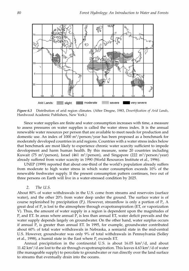
80 Forest Hydrology: An Introduction to Water and Forests
Since water supplies are finite and water consumption increases with time, a measureto assess pressures on water supplies is called the water stress index. It is the annualrenewable water resources per person that are available to meet needs for production anddomestic use. An index of 1000 m
3
/person/year has been proposed as a benchmark formoderately developed countries in arid regions. Countries with a water stress index belowthat benchmark are most likely to experience chronic water scarcity sufficient to impededevelopment and harm human health. By this measure, some 20 countries includingKuwait (75 m
3
/person), Israel (461 m
3
/person), and Singapore (222 m
3
/person/year)already suffered from water scarcity in 1990 (World Resources Institute et al., 1996).
UNEP (1999) reported that about one-third of the world’s population already suffersfrom moderate to high water stress in which water consumption exceeds 10% of therenewable freshwater supply. If the present consumption pattern continues, two out ofthree persons on Earth will live in a water-stressed condition by 2025.
2. The U.S.
About 80% of water withdrawals in the U.S. come from streams and reservoirs (surfacewater), and the other 20% from water deep under the ground. The surface water is ofcourse replenished by precipitation (P
t
). However, streamflow is only a portion of P
t
. Agreat deal of P
t
is lost to the atmosphere through evapotranspiration (ET, or vaporizationV). Thus, the amount of water supply in a region is dependent upon the magnitudes ofP
t
and ET. In areas where annual P
t
is less than annual ET, water deficit prevails and thewater supply depends largely on groundwater. On the other hand, water surplus occursif annual P
t
is greater than annual ET. In 1995, for example, groundwater contributedabout 60% of total water withdrawals in Nebraska, a semiarid state in the mid-centralU.S. However, groundwater was only 9% of total withdrawals in Pennsylvania (Solleyet al., 1998), a humid state in the East where P
t
exceeds ET.Annual precipitation in the continental U.S. is about 16.05 km
3
/d, and about11.42 km
3
/d are lost to the air through evapotranspiration. This leaves 4.63 km
3
/d of water(the manageable supply) to percolate to groundwater or run directly over the land surfaceto streams that eventually drain into the oceans.
Figure 6.3
Distribution of arid region climates. (After Dregne, 1983,
Desertification of Arid Lands
,Hardwood Academic Publishers, New York.)
1363_C06_fm Page 80 Wednesday, December 4, 2002 7:41 AM
Chapter six: Water resource problems 81
Of the 1.52 km
3
/d total water withdrawals in 1995, about 1.22 km
3
/d were surfacewater (Table 6.2). This was about 26% of annual runoff. The remaining 74% or 3.41 km
3
/dwere available to supply additional growth in water demand. The projected surface waterwithdrawals in 2040 made by the U.S. Forest Service are 1.55 km
3
/d. U.S. water suppliesshould be adequate to meet this demand.
Although overall the U.S. seems to have plenty of water to meet demand in the future,a large region of the U.S. has experienced water shortages every year due to unevendistribution of population, industry, agriculture, and available water. A deficit of waterexists where potential evapotranspiration is greater than precipitation, or demand forwater is greater than supply. These areas lie generally west of the 96th meridian and eastof the Rocky Mountains. Here annual precipitation is generally less than 60 cm, and surfacerunoff of less than 10 cm occurs only during or immediately after storms, except areas inhigher mountains. Table 6.4 shows that the 17 western states have 33%, or 544 km
3
/year,of the total runoff in the contiguous U.S., but the West withdrew 44% or 240 km
3
of thenation’s streamflow in 1990. The greatest demand for water in the West is agriculturalirrigation, and in the East it is for industry purposes. These uses, respectively, make up82% of total off-stream withdrawals in each region.
The precipitation regime of a region is affected by (1) position relative to air-massmovement and moisture content of the air, (2) proximity to major pressure systems, and(3) elevation and other topographic characteristics. The U.S. is located in a region of Earththat is influenced by the westerlies (prevailing winds blowing from west to east). Majortracks of storms and weather fronts move from the Pacific Ocean and the Gulf of Mexicoto the Atlantic Ocean. These cause the windward (western) slopes of the Rocky Mountainsand the Northern Pacific coastal plains to record the greatest precipitation in the U.S. They
Table 6.4
Total Water Withdrawals, Population, and Per Capita Use of Water between
the Eastern (31 States) and Western (17 States) U.S. in 1990 and Their Normal Runoff
Items
Western States
Eastern States Total VolumeVolume % Volume %
Water withdrawals, km
3
/dSurface Water
Fresh 0.4158 41.4 0.5810 58.6 0.9968Saline 0.0548 25.6 0.1583 74.4 0.2132Sum 0.4707 30.9 0.7393 69.1 1.2100
GroundwaterFresh 0.1833 64.0 0.1031 36.0 0.2864Saline 0.0037 94.9 0.0002 05.1 0.0039Sum 0.1870 64.4 0.1033 35.6 0.2903
TotalFresh 0.5991 59.9 0.6841 40.1 1.2832Saline 0.0586 27.0 0.1585 73.0 0.2171Sum 0.6577 43.8 0.8426 56.2 1.5003
Per Capita, m
3
/dFresh 7.1353 3.8529 4.9088Total withdrawals 7.8431 4.7455 5.7391
Population, thousands 83,853 32.1 177,563 67.9 261,416Runoff (1931–1960), km
3
/d 1.4898 32.8 3.0522 67.2 4.5420
Note:
Percents in rows total to 100.
Sources:
Data for water withdrawals and population were calculated from Solley, W.B., Pierce, R.R., and Perlman,H.A., 1998, Estimated use of water in the United States in 1995, U.S. Geological Survey Circular 1200, Wash-ington, D.C. Runoff data were calculated from Murray, C.R., 1968, Estimated use of water in the United States,1965, U. S. Geological Survey Circular 556, Washington, D.C.
1363_C06_fm Page 81 Wednesday, December 4, 2002 7:41 AM
82 Forest Hydrology: An Introduction to Water and Forests
are followed by the Gulf Coast around the mouth of the Mississippi River, southeastFlorida around West Palm Beach, and the high mountain plateau of western North Caro-lina. Annual precipitation for the community of Forks on the western side of the OlympicMountains, Washington, is about 3000 mm, but it drops to about 450 mm at Port Townsend,only 120 km away on the leeward (eastern) side of the same mountains.
The Intermountain region and the Southwest are in a rain-shadow created by theCascade Range and Coast Ranges to the west. The Coast Ranges block the influx of warmmoist-air masses moving from the Pacific. Also, moist-air masses from the Gulf of Mexicoand the Atlantic gradually lose moisture as they travel inland. These factors cause theSouthwest and the Intermountain regions to be the driest in the nation. Normal annualprecipitation is only about 100 mm at Yuma, an Indian Reservation near the border ofArizona, California, and Mexico. The seasonal precipitation distribution for a few selectedlocations in the U.S. is shown in Figure 6.4.
II. Water quantity
A. Drought
When water demand is greater than supply, water shortage occurs. If the shortageextends over a significant period of time, it is a drought. However, water shortage canapply to agriculture, to water level in the rivers and reservoirs, or to human comfort asa result of lack of rainfall, high temperature, and low humidity. Thus, drought has beendefined through meteorological, agricultural, hydrological, or even socioeconomicpoints of view. It means different things to different people and varies from region toregion. In equatorial areas, a week without rain is a drought, while such a period canextend to 2 years in Libya.
Unlike floods, drought occurs slowly, grows gradually, and acts silently. There are noexciting violent occurrences or immediate disruptions of life and social order associated
Figure 6.4
Seasonal precipitation distribution for selected locations in the U.S.
1363_C06_fm Page 82 Wednesday, December 4, 2002 7:41 AM
Chapter six: Water resource problems 83
with drought. The damages of drought are chronic. But once it becomes noticeable, it mayhave already caused tremendous losses in agriculture, reductions in economic growth,increases in food prices, and problems of infestation associated with insects, fungi, bacteria,and viruses, which in turn may shift farming practices and life-styles. Drought is not justa natural phenomenon affecting only crops or water supplies. The effects of drought coverall aspects of life and are much more profound and widespread than those of floods.
No panacea can be used with economic feasibility to fight effectively against drought.Although elimination of drought is unattainable, numerous measures have been devel-oped to cope with shortages of water and reduce drought damage. These measures eitheraugment water supply or conserve water use and work better when applied in concert.They include:
1. RainmakingArtificially induced rain or snow would be an ideal solution to droughts especially ifprecipitation timing, location, and amounts could be controlled. Rainmaking is done bycloud seeding with crystals of dry ice, silver iodide, salts, or even clay particles when rainclouds are present in the sky. Experience in the U.S. shows that such activities couldincrease precipitation on the order of 10 to 50% in some regions, with no significantincreases or even decreases in precipitation in other regions. Much of the uncertainty isdue to the nature of precipitation variability (MIT, 1971).
Besides the uncertainty problem, the fact that rain clouds are a requirement makesrainmaking inapplicable in very dry areas where such clouds are rarely available. Inaddition, using these clouds may create legal disputes over their ownership. As water isremoved from clouds in one area, it could deprive neighboring areas of water. Large-scaleapplication can cause changes of regional or even global weather patterns in undesirableways. A cloud-seeding experiment conducted near Rapid City, South Dakota, in thesummer of 1972 was allegedly responsible for the subsequent 356 mm of rain and floodingthat followed (Owen, 1985). The usefulness of rainmaking is limited by a lack of controlover the volume, intensity, and distribution of resulting precipitation.
2. Water translocationThe distribution of freshwater supplies in nature is very uneven geographically. Cities areexpanding, becoming so large that water supplies are not sufficient for their demands;agricultural irrigation is always needed in arid areas but water is in limited supply. Aconventional solution to the water shortage is to transport water from an area of surplusto an area in need through pipelines, channels, canals, trucks, etc., depending on distanceand quantity.
Libya is located in North Africa with the Mediterranean Sea on the north, Egypt andSudan on the east, and Chad and Niger on the south. About 95% of the country is desert,and the average annual rainfall is 26 mm with only 7% of the land exceeding 100 mm/year.The arid climate leads Libya to rely on water stored in reservoirs during wet years and
Water Augmentation Water ConservationRainmaking Household conservationWater translocation Evaporation reductionDesalination Irrigation efficientWater reclamation Vegetation controlRain harvesting (Water storage) Genetic engineeringIceberg harvesting Drought forecast
Price control
1363_C06_fm Page 83 Wednesday, December 4, 2002 7:41 AM
84 Forest Hydrology: An Introduction to Water and Forests
in underground aquifers for its water supply. In 1986 Libya initiated the “Great ManmadeRiver Project” to pump water out of aquifers deep beneath the Sahara desert formed 20,000to 40,000 years ago. Some 4000 km of pipeline with a diameter of 4 m, buried 6 to 7 munder the ground, will stretch from the desert to cities along the Mediterranean (Borrell,1986; Jordaan et al., 1993). The project consists of five phases with a total volume of water2 km3/year to be transported for a period of at least 50 years. It is expected to meet thedemands for water for the heavy population along the coast and to irrigate nearly200,000 ha of agricultural land. The first phase was completed in 1997. Tapping the deepaquifers has raised concerns that smaller pockets of water close to the surface and scatteredoases may disappear. As a result, large areas of desert may be depopulated and thetraditional way of life of its nomadic inhabitants destroyed.
The North American Water and Power Alliance (NAWAPA) proposed to make allmajor rivers in Alaska and northwest Canada run backward so that water could bepumped and directed into 7 provinces in Canada, 33 states in the U.S., and 3 states inMexico. The scheme was to build massive dams on most north-flowing rivers above the55oN latitude. Thousands of kilometers of beautiful valleys would be permanently floodedto create gigantic reservoirs, 15 of them larger than Lake Mead, the largest artificial lakein North America. NAWAPA would take 20 to 30 years to construct with an estimatedcost of $100 billion in 1964 (Mather, 1984).
Perhaps the most complex and expensive water-translocation project in the U.S. isCalifornia’s aqueduct system. About 70% of California’s potentially usable water origi-nates from the northern third of the state, while 77% of the demand comes from thesemiarid southern two-thirds of the state. A dam of 235 m height blocks water in theFeather River in the North to form Lake Oroville with a capacity of 4.32 ¥ 109 m3 and213 m deep. The water is then alternately translocated toward Los Angeles, San Diego,and the San Fernando Valley through 21 dams, 22 pumping plants, and 1046 km of canals,tunnels, and pipelines (California Department of Water Resources, 1973). The project hasbeen criticized for its excessive costs in construction and energy, losses in scenic beautyand free-flowing wild rivers, and the destruction of fish and wildlife habitats (Owen, 1985).
New large-scale water-transfer projects are increasingly difficult to establish because(1) political and environmental issues will create lengthy delays, (2) the costs will beextremely high, (3) the construction time is too long, (4) smaller projects or other approacheswith fewer environmental-impact issues will be more attractive to policy-makers, and(5) environmental groups will insist on greater water use efficiency prior to construction.
3. DesalinationSaline water includes brackish water (1000 to 4000 mg/liter of dissolved solids), saltedwater (4000 to 18,000 mg/liter), seawater (18,000 to 35,000 mg/liter), and brine water(more than 35,000 mg/liter). With seawater accounting for more than 97% of the world’stotal water budget, converting the saline water into usable water seems to be a logicalalternative for augmentation of water supply. Technologically, the conversion can be doneby use of distillation processes or reverse osmosis. Commercially, the techniques are notyet in widespread use because of energy requirements, costs, and environmental con-straints such as waste disposal problems, heat, and other air pollutants. Desalted watercosts about $1 per 1000 gal (3.785 m3) compared to $0.25 to $0.40 per 1000 gal for tapwater. In 1999, desalination capacity of the world was about 0.021km3/d (0.15% of waterconsumption) and 75% of the capacity was in ten countries (Gleick, 2000).
4. Water reclamationSewage wastes have long been used to irrigate agricultural crops and, more recently,forested lands as a provider of both moisture and fertilizers in areas where water supplies
1363_C06_fm Page 84 Wednesday, December 4, 2002 7:41 AM
Chapter six: Water resource problems 85
are limited (Stulp, 1995). Although many people are concerned about aesthetic effects andabout the possible transmission of viruses and other contaminating organisms, wasteeffluents in fact can be treated to yield a quality suitable for many uses, including bodycontact. Such processed sewage water has already been used for a variety of functions,including irrigation, steel cooling, groundwater recharging, aquaculture, creation of con-structed wetlands, streamflow augmentation to enhance salmon runs and to improvewater quality, recreational lakes, and domestic and industrial supplies.
As new water resources and transfer projects become more difficult to develop,reclaimed water provides an economical source to ease our water-supply constraints. Italready has become a safe, reliable, and drought-proof source of nonpotable water for aridstates such as California, Arizona, Nevada, and Florida. In 1992, the state of Washingtonpassed the Reclaimed Water Act (codified as RCW 90.46) to encourage beneficial use ofreclaimed water for various applications. The reclamation and reuse system created bythe city of Yelm, Washington, is a success story (Skillings, 1999). The system totallyeliminates the discharge of wastewater into the Nisqually River to protect water qualityand salmon habitat and the city’s groundwater resources, and provides water for publicuses such as ground watering, vehicle washing, and a wetland park.
5. Rain harvestingIn rain harvesting, rainwater is captured to increase water availability for crop production,gardening, household, livestock, or other uses. Methods include trapping more runoffthrough land-surface treatments, collecting rainwater from roofs, increasing snow accu-mulation through snow fences, terrain modification and forest management practices, andcatching fog and cloud drips in coastal areas or at tops of mountains by installing artificialscreens. Some techniques for harvesting rainwater from roofs and ground catchmentswere described by the United Nations Environment Programme (1983).
Land surfaces can be treated to produce more runoff water by digging ditches to catchwater from hillsides and directing the water to a pond for various uses. The ditches mustbe on soils with low water permeability; otherwise the soil needs to be treated with sodiumsalts, or spread with water-repellent compounds such as asphalt, paraffin, latex, or sili-cones. One can use large sheets of plastic or Agri-fabric, a nonwoven engineering geotextilemade from 100% Trevira polyester, to cover the entire runoff-producing area and thestorage reservoir. To reduce evaporation losses, the reservoir should be deep rather thanlarge in surface area. Rainwater can also be harvested from house roofs using gutters,drains, or troughs and stored in tanks (cisterns). These are all ancient practices and canbe applied in areas where average annual rainfall is as low as 50 to 80 mm. In the U.S.Virgin Islands roof rainwater-catchment systems are quite common, and local ordinancesspecify catchment areas and storage volumes (Sharpe, 2001). Systems like these have beenpromoted in urban areas to provide water for landscape maintenance. Several publicationsare available that provide methods for calculating necessary roof areas and storage vol-umes based on rainfall amounts (Young and Sharpe, 1989).
In alpine areas, snowfall is the most important type of precipitation and the domi-nating factor in the yield and timing of streamflow. Intensive management of alpineforests and snowfields offers excellent opportunities for increasing snow accumulationand delay of snowmelt, and consequently augmenting water yields. Along coastal areasor fog-prone regions, reversing the effect of rainfall interception can be observed due tocondensation of fog or cloud moisture on the forest canopy, dripping to the ground asadditional rainwater (Goodman, 1985). Arranging lattices and nets above woods in Japanhas collected as much as 20 times more water on the windward than on the leeward side(Ooura, 1952). Under an old-growth Douglas-fir forest near Portland, Oregon, fog dripcould add an additional 882 mm of water to total precipitation during a year (Harr, 1982).
1363_C06_fm Page 85 Wednesday, December 4, 2002 7:41 AM
86 Forest Hydrology: An Introduction to Water and Forests
Accordingly, loss of fog drip due to patch clearcutting of the watershed could cause asignificant decrease of streamflow in the summer (Ingwerson, 1985).
A fog-collection system of 75 polypropylene nets was installed to capture water dropsat Chungungo, Chile. The trapped water was directed into troughs where the water waschlorinated. It was then fed into a gravity system that descended to the village througha 6.5 km pipeline. Before the system was installed, each villager lived on 13 l of water perday delivered by trucks once a week. Now, the fog-collection system furnishes eachresident 53 l of water a day at half of the previous cost (U.S. Water News, 1994).
The barrel-shaped baobab trees (Adansonia digitata) of tropical Africa have trunks upto 9 m in circumference. Some tribesmen hollow out the trunks of these trees for housesand commercial stores or for water storage. In Sudan, people dig a moat around a baobabtree for rain harvesting. The harvested rain is then bucketed, as much as 4 m3, into thehollow trunk for storage.
6. Iceberg harvestingMore than 77% of the world’s freshwater is locked up in ice, mostly in Antarctica and inthe Arctic. If the ice could be melted and drained into reservoirs, there would be enoughwater to supply our needs for more than 7000 years at the present withdrawal rates.Icebergs in Antarctica are broad and flat, resembling giant float tables or ice islands. Itmay be economically feasible to tow Antarctic icebergs to Southern California, SouthAmerica, Saudi Arabia, Australia, or other coastal places with oceangoing tugs aided bythe favorable Humboldt Currents. These icebergs would then be melted and piped inlandfor domestic, industrial, or agricultural purposes. The idea received considerable attentionwhen the First International Conference and Workshop on Iceberg Utilization was heldat Iowa State University in Ames, Iowa, in 1978 (Husseiny, 1978). However, there are someproblems regarding the utilization of icebergs: (1) the ownership of icebergs, (2) theenvironmental effects on coastal water temperature, fish reproduction, and migration aswell as on climatic patterns, and (3) the hazards that might be created if chunks of icebergswere broken off in international shipping lanes. It is unlikely that the intriguing idea willbe implemented in the near future. But as water shortages continue to grow and theoperational technology is further developed, icebergs provide a new water resource thatwill meet our water demands for a long time.
7. Household conservationAbout 30 to 50% of the water used in the U.S. is wasted unnecessarily. Water conservationmeans using water wisely, increasing the efficiency and reducing waste. Thus, householdconservation involves the use of technologies, practices, policies, and education to reduceper capita use of water by people in drinking, cooking, bathing, toilet flushing, lawnwatering, fire protection, swimming pools, car washing, laundering, and washing dishes.Much of the water around individual homes is wasted due to poor habits, lack of concern,or inefficient plumbing fixtures. A slow drip from faucets can waste as much as 650 l ofwater each day or 240 m3 each year. Texas Water Development Board (1994) has shownhow household water consumption can be reduced in a brochure called “Forty-nine watersaving tips.” Frequently, city ordinances are required to help govern plumbing codes, lotsizes, drainage grades and slopes, or outdoor usage, which can reduce the quantity ofwater used. Nationally, legislation was passed in 1992 requiring water-efficient plumbingfixtures (Energy Policy Act of 1992).
8. Evaporation reductionAnnual lake evaporation in the U.S., excluding Alaska and Hawaii, ranges from about500 mm in the north of Maine to 2000 mm in the southwest of Texas (U.S. Weather Bureau,
1363_C06_fm Page 86 Wednesday, December 4, 2002 7:41 AM
Chapter six: Water resource problems 87
1959). Saving 10 mm of water from a reservoir of 50,000 ha in size is sufficient to supplydomestic water to 50,000 people for more than 5 months. Reservoir evaporation can bereduced by reducing the evaporation surface, by application of mechanical covers to itssurface, or by spreading the surface with thin films of chemicals. The surface-film methodis the simplest and the most economical for evaporation reduction. Chemicals used forthis purpose must be insoluble, nontoxic, pervious to oxygen and carbon dioxide, pene-trable by raindrops, flexible with motion of the water surface, and inexpensive. Dependingon wind effects, type of chemical, and the conditions under which it is used, normalevaporation can be reduced as much as one-third by efficient use of monofilms.
9. Irrigation efficiencyWater loss due to inefficient agricultural irrigation is another important item in waterconservation. As much as 50% of the irrigated water is not used by crops due to evapo-ration loss or seepage. Improving the efficiency of existing irrigation practices can increasecrop yields, reduce weed growth, and cut irrigation water by 50 to 60%. The methodsinclude: (1) better scheduling of water application (based on real-time soil moisture andmeteorological conditions), (2) use of closed conduits in water-conveyance systems,(3) using trickle or drip irrigation systems to apply water directly into the roots of plantsrather than flooding the entire area, (4) reducing irrigation water runoff by using contourcultivation and terracing, and storing runoff water for use in farm ponds or small lakes,and (5) covering the soil with mulches.
10. Vegetation controlBecause of surface area, deep root systems, more available energy, and wind effects, waterlosses from vegetated watersheds are greater than if the same area were bare ground.Plant size, canopy density, roots, and leaf characteristics vary among species, resulting invariable transpiration losses. Thus, vegetation management, especially on phreatophytesand forested watersheds, provides promising opportunities to reduce water loss, andconsequently augment water yield.
Phreatophytes are water-loving plants whose roots penetrate into the groundwatertable or spread widely for possible sources of water. They represent the most seriousproblem in water management in semiarid and arid regions. In Texas one such plant,mesquite, grows in drainage ways with annual rainfall of 15 cm extending to beyond 75cm. Its roots penetrate the soil more than 5 m deep and spread as much as 15 m from itstrunk, transpiring a luxurious amount of water to the air. Another plant, saltcedar, growsextensively in 15 of the 17 western states. It forms an almost continuous band of vegetationalong many rivers and streams. Saltcedar not only consumes a large quantity of water(possibly reaching 2700 mm/year), but also chocks river beds with vegetation and sedi-ment, thereby increasing flooded areas and peak flows. An elimination of saltcedar growthfollowed by grassland restoration might result in a collective net water saving of300 mm/year (Texas Water Development Board, 1968). Other species of such water-wast-ing plants include cottonwood, elm, post oak, black oak, live oak, shin oak, whitebrush,sagebrush, sassafras, cactus, juniper, yaupon, retama, and willow.
Forests transpire more water than other types of vegetation. Water yield can thus beincreased by manipulation of forests without increasing surface runoff and soil erosion.The method is to reduce transpiration by (1) converting vegetation from species that usemuch water to species that require less water, (2) clearcutting or partial cutting of theforest, (3) reducing forest densities, and (4) using antitranspirants. Many managementmethods, including conversions of chaparral to grass, tree to grass, tree to shrub, andhardwood to conifer, or forest clearcutting, patch cutting, understory cutting, and thinning,have been tested in small watersheds for their effects of streamflows. The results show an
1363_C06_fm Page 87 Wednesday, December 4, 2002 7:41 AM
88 Forest Hydrology: An Introduction to Water and Forests
increase in streamflow ranging from 30 to 540 mm/year, depending on annual precipita-tion, vegetation, management, and physiographic factors.
Since most of the vegetation-management studies were conducted in small water-sheds, it is uncertain how much water can be increased from large watersheds, and whenand how that water will be released. Upstream forest manipulation results in increases ofwater yield downstream. Frequently, the landowners and beneficiaries are different peo-ple, especially when large watersheds are involved. Until the legal problems are solved,and objective models for evaluating input and output components of water augmentationprojects over a broad range of environmental conditions have been developed, validated,and accepted by the courts, the approach, if carried out, will inevitably be restricted topublic lands. Private forest owners will not base their management strategies on waterproduction. Moreover, the method is inapplicable in areas where annual rainfall is lessthan 500 mm, or topography is so rugged and fragile that clearcutting would create severesoil-erosion problems.
11. Genetic engineeringThrough research and experiments in genetics, it may be possible to breed plants thatrequire considerably less water or grow well in saline soils. Once these salt-resistant anddrought-resistant crops are developed, seawater can be used for irrigation and vast areasof arid or semiarid regions can become productive. A new saltwater barley developed bytwo scientists from the University of California at Davis grew well on a tiny windsweptbeach with a yield of 1500 kg/ha (Owen, 1985). There are 1.8 ¥ 106 ha of once-primeagricultural land in California that are worthless now due to the salinization caused byimproper irrigation practices or seawater intrusion. The new barley could be expected todo well in this type of soil.
12. Drought forecastLow-flow information is essential for reservoir design, the management of water-supplysystems, and the study of the waste-assimilative capacity of streams. A common criterionfor these purposes is the average lowest 7-day, 10-year flow. Information on the probabilityof occurrence of droughts with various severity and duration during a single year orduring any specific period of years can be statistically analyzed using historical recordsof precipitation and streamflow. The severity of droughts can be measured by parameterssuch as deficiencies in rainfall and streamflow, declines in soil moisture and groundwaterlevel, persistence of rainless days, various drought indexes, and the storage required tomeet prescribed withdrawals. Analysis of past records indicates that the sequence of dryyears is not random, and a prolonged drought in the Western U.S. occurs about every 22years. Large-scale studies on the distribution, occurrence, severity, and duration ofdroughts may provide clearer insight and more reliable information to help us to preparefor problems in the future, including addressing them with conservation programs andwater storage.
13. Price controlWater has been priced at reproduction costs in the past. However, most systems charge aminimum price for a given quantity of water with a decreasing price for additional use,while others charge a minimum price with an increasing rate for additional use. Otherwater systems charge a uniform rate that is independent of use. Innovative increasingblock rates have been adopted in many municipalities to encourage conservation (Younget al., 1983). When water-supply savings are added to sewer and energy costs, consumersavings can be substantial.
1363_C06_fm Page 88 Wednesday, December 4, 2002 7:41 AM
Chapter six: Water resource problems 89
B. Floods
An inundation or overflow of the floodplain of a river, which causes substantial loss oflife, personal property, public facilities, or agricultural productivity, is called a flood. Floodsare the number one killers among natural disasters. A flood that occurred along the YellowRiver (Huang Ho), China, in 1931 inundated 1.1 ¥ 105 km2, caused 1 million fatalities, andleft 80 million people homeless. The death toll outnumbered any other major naturaldisaster known today, including the earthquake of Tangshan, China, in July 1976 (800,000lives), the cyclones of Bangladesh in November 1970 (300,000 lives), and the tornadoes ofMissouri, Illinois, and Indiana on March 18, 1925 (689 lives).
Floods occur in various forms: flash floods, river floods, urban floods, and coastalfloods. Each type has features different from the others. Knowing the characteristics ofthese floods can help us prepare for the threat and reduce the damage to a minimum level.
1. Forms and causes
a. Flash flood. Flash floods occur in mountain streams, upper tributaries, or can-yons with relatively small watershed areas. Small watersheds have smaller water-storagecapacity than large watersheds. The water-storage capacity refers to the ability of a water-shed to keep water or delay the movement of water within its drainage system throughvegetation, land surface, topography, soil profiles, and stream channels. Thus, smallerwatershed storage means that water moves out of the watershed faster and in greatervolume per unit area.
Most flash flooding is associated with slow-moving thunderstorms, intensive rainsfrom hurricanes, tropical storms, a sudden release of water from snowpacks, or a collapseof dams and levees. Generally, thunderstorm activities are of high intensity, short duration,and small area. If the rate of an intense rain is greater than the storage rate of a watershed,the excessive rainwater will become overland flow and run to nearby stream channels.When thunderstorms occur in upper tributaries, which have small watershed-storagecapacity, overland flow from every portion of the watershed can arrive in stream channelsin a short period of time. The enormous amount of water can easily exceed the channelcapacity, resulting in flooding of its floodplain areas.
Flash floods can rise to a height of 10 m or more in a few minutes or hours. Thesewaters move at very fast speeds with a roar like running horses and are accompanied bysediment, rocks, stones, and a variety of debris. Floodwaters can travel to downstreamareas where there are no storm activities at all. They uproot trees, destroy buildings, andwipe out bridges. They occur with little or no warning, and retreat rapidly.
b. River flood. Unlike flash floods, river floods occur along major rivers and inlower tributaries of large watersheds. Since it takes more time for water to travel throughlarge watersheds, the crest of a river flood can arrive at a downstream location in a fewdays or even weeks after storms. Similarly, floodwaters can stay in floodplains for daysor weeks before completely draining.
River flooding is associated with torrential rains in spring, heavy thunderstorms,hurricanes, tropical storms, and snow thaws. If waters generated from these storms inthe watershed exceed the capacity of river channels, flooding results. Because the groundis usually saturated or frozen, a severe storm occurring in winter has a greater potentialfor flooding than if it occurs in summer. Sometimes a failure of dams, or a jam of ice,can cause severe flooding. The failure is usually the result of negligence, poor manage-ment, inadequate design, or structural damage. Water from a collapsed dam sweepseverything downstream.
1363_C06_fm Page 89 Wednesday, December 4, 2002 7:41 AM
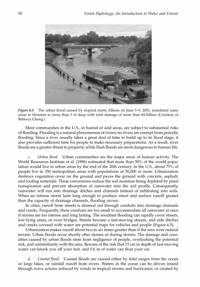
90 Forest Hydrology: An Introduction to Water and Forests
Most communities in the U.S., in humid or arid areas, are subject to substantial risksof flooding. Flooding is a natural phenomenon of rivers; no rivers are exempt from periodicflooding. Since a river usually takes a great deal of time to build up to its flood stage, italso provides sufficient time for people to make necessary preparations. As a result, riverfloods are a greater threat to property, while flash floods are more dangerous to human life.
c. Urban flood. Urban communities are the major areas of human activity. TheWorld Resources Institute et al. (1996) estimated that more than 50% of the world popu-lation would live in urban areas by the end of the 20th century. In the U.S., about 75% ofpeople live in 350 metropolitan areas with populations of 50,000 or more. Urbanizationdestroys vegetation cover on the ground and paves the ground with concrete, asphalt,and roofing materials. These conversions reduce the soil moisture being depleted by planttranspiration and prevent absorption of rainwater into the soil profile. Consequently,rainwater will run into drainage ditches and channels instead of infiltrating into soils.When an intense storm lasts long enough to produce street and surface runoff greaterthan the capacity of drainage channels, flooding occurs.
In cities, runoff from streets is drained out through conduits into drainage channelsand creeks. Frequently, these conduits are too small to accommodate all rainwater at onceif storms are too intense and long lasting. The resultant flooding can rapidly cover streets,low-lying areas, or even bridges. Streets become a fast-moving stream, and side ditchesand creeks covered with water are potential traps for vehicles and people (Figure 6.5).
Urbanization makes runoff about two to six times greater than if the area were naturalterrain. Urban floods occur shortly after storms or during storms. The damage and casu-alties caused by urban floods stem from negligence of people, overlooking the potentialrisk, and unfamiliarity with the area. Beware of the risk that 15 cm in depth of fast-movingwater can knock you off your feet, and 0.6 m of water can float your car.
d. Coastal flood. Coastal floods are caused either by tidal surges from the oceanor large lakes, or rainfall runoff from rivers. Waters in the ocean can be driven inlandthrough wave actions induced by winds in tropical storms and hurricanes, or created by
Figure 6.5 The urban flood caused by tropical storm Allison on June 5–9, 2001, inundated someareas in Houston to more than 3 m deep with total damage of more than $4 billion (Courtesy ofRebecca Chang.)
1363_C06_fm Page 90 Wednesday, December 4, 2002 7:41 AM
Chapter six: Water resource problems 91
earthquakes and volcanic activity. When an earthquake or volcanic activity occurs in theocean, the created waves, called tsunamis, can travel in all directions for thousands ofmiles. These waves, depending on how deep they are in the ocean, can be 30 m or morein height, as short as 1500 m in length, and travel up to 800 km/h. A tsunami can travelfrom one side of the Pacific to the other in less than one day, or it can hit a coastal areain a few minutes. They are not very tall when they are traveling in the water, but canbecome tall when they strike the land.
Tsunamis are very destructive. They carry away people, animals, objects, and boats,wipe out villages, and flood the area for weeks.
2. Nature of floodsFloods can be measured for their elevation, area inundation, peak discharge, volume offlow, and duration. The size of these variables depends upon the rate, duration, distribu-tion, and direction of the storm as well as the weather and the condition of the ground onwhich it falls. Thunderstorm activity and intense storms are predominantly warm-seasonphenomena in the U.S. However, no specific intensity of storm or rate of flow will causeflooding. What may be a flood at one section of the river may be well-controlled flow atanother section. The flood-producing potential of intense storms is much greater duringwinter and in urban areas. When unexpected storm intensities occur during cold seasons,especially during late winter, streamflow rates may be maximum, and where there is nocanopy interception or transpiration in hardwood forests, evaporation is negligible, andthe soil possibly frozen or highly saturated, the results are frequently disastrous.
When an abnormally warm temperature, which can melt much of the snowpack, isfollowed by an intense storm in the cold season, flooding results are frequently disastrous.Paved streets prevent rainwater from entering into soils, and the removal of trees in urbanareas reduces transpiration loss of water from the soil. Consequently, runoff in urbanizedareas can be two to six times over what would occur on natural terrain.
The hydrological behavior of watersheds varies with basin sizes. In small tributariesor upstream areas, the average slope steepness is greater, the average rainfall intensity ishigher, the soil depth is shallower, the watercourse is shorter and steeper, and the variablesof climate may be more extreme than in large watersheds. Thus, small watersheds arevery sensitive to high-intensity rainfalls of short duration and can be greatly affected byland use. Floods in small watersheds are characteristically flash floods of short durationand high peak flows per unit area. On large watersheds, the effect of channel flow or basinstorage is the dominant factor in flood hydrographs. Thus, if flood flows from severalsmall tributaries arrive at the main stream at about the same time, a major flood can occur.Major floods do not occur in direct response to storm intensity. They occur gradually anddrain out slowly.
3. Flood damagesPeople can be drowned in floodwaters or indirectly killed by flood-induced fire, diseases,or even animal attack. In India and Pakistan, as reported by Time magazine (Clark, 1982),“people seeking refuge in treetops have died in agony from the bites of venomous snakes.”Similarly, property damages can be direct, indirect, or intangible. Direct losses apply tothose items that can be determined in cash value, while indirect losses are those, such asproperty depreciation and loss of business or job, caused by the effects of flooding.Intangible losses include damages to environmental aesthetics, environmental hazards,loss of ecological habitat, migration of population, or crime activity that cannot be assessedby cash value. The assessment of flood losses is not an easy job. For example, floodingcan cause substantial soil erosion and consequently soil deposition on crop fields, streets,
1363_C06_fm Page 91 Wednesday, December 4, 2002 7:41 AM
92 Forest Hydrology: An Introduction to Water and Forests
buildings, reservoirs, and many other locations. In Bangladesh, the raging floodwaters inthe summer of 1998 submerged tens of thousands of wells across the country, making thewell water undrinkable. The government reported nearly 194,000 cases of diarrhea andat least 160 deaths. Thus, the damages may include loss of crops, costs due to the cleanoutof soil deposition, depletion of land productivity, degradation of water quality, reductionof reservoir capacity, and impairment of landscape aesthetics.
River flooding can deliver a large quantity of freshwater to the ocean, dilute the ocean’ssalinity level, and consequently affect marine biology. For example, the 1998 summer floodthat occurred along the middle and lower Yangtze River is the biggest recorded in Chinain the 20th century. It lasted more than 60 days, drowned more than 1300 people, andcaused a direct economic loss exceeding 177 billion Chinese yuan. The floodwaters pouredinto the Yellow Sea, drifted to the Cheju Island, South Korea, and reduced the island’ssalinity level from 3.1% to 2.5%. It was reported that the island’s marine shellfish farmingwas already reduced by 30% during the Yangtze River’s flood of August 1996.
Flood damages can also cause the disruption of communication and transportationsystems as telephone lines go down, bridges are washed out, and highways and railroadtracks are torn apart. Broken power lines and ruptured gas mains can cause fire, rats anddead animals can spread diseases, and floodwaters can be contaminated from sewers,animal feedlots, and other sources. If flooded areas are not treated properly and promptly,epidemic diseases can prevail. After the livestock and crops are wiped out, famine canmenace the land. Many of these effects can take months or even years to assess fully.
a. Flood damages increase with time. Property losses caused by flooding in theU.S. increased from $1,484,000,000 in 1936–1945, to $2,721,000,000 in 1956–1965, to$21,493,000,000 in 1976–1984. Between 1986 and 1995 the annual loss from flood damagein the U.S. ranged from $24 million in 1986 to $16,370,000,000 in 1993 with an average of$3,550,000,000 per year.
As population increases exponentially with time, so does utilization of and develop-ment in floodplain areas. The concentration of population and intensive developmentalong the floodplain makes property values higher and the potential flood damage greater.Moreover, the utilization of groundwater to meet water demands for population increaseoften causes a subsequent land subsidence, resulting in more areas that are subject toflooding. In the past, flash floods in the Eastern U.S. were often associated with storms of4 in. (about 10 cm) or greater (Maddox and Chappel, 1979). Now, floods occur in manyareas with a storm of only 2 in. (about 5 cm) or greater.
b. Losses per unit area decrease with increasing watershed size. Streamflow phe-nomena and behavior are quite different between large watersheds and small watershedsdue to their environmental conditions. A large watershed usually implies a condition inwhich watershed slope, rainfall intensity, flow velocity per unit area, and the chances ofgetting the entire watershed covered by storms are smaller, soil is deeper, and watershedstorage is greater. Small watersheds are very sensitive to land-use conditions and to stormsof high intensity and short duration. This means that the increase of streamflow in responseto storm rainfall is more rapid for small or bare watersheds than for large or forestedwatersheds. Stream sedimentation and flow volume per unit area decrease with increasingwatershed area, as do flood damages.
c. Forested watersheds are less damaging. Forests are the most distinguished typesof vegetation on Earth. Their large and thick canopies, fluffy forest floor, and deep rootsystems impose tremendous effects on water, soil, and nutrient movements within thewatershed. For example, forested watersheds transpire a great deal of water to the air, cut
1363_C06_fm Page 92 Wednesday, December 4, 2002 7:41 AM
Chapter six: Water resource problems 93
down the amount of rainwater to reach mineral soils, increase soil water holding capacity,and reduce overland flow velocity and soil-erosion losses (Anderson et al., 1976). Thesemake flood damages in forested watersheds less than those in agricultural or urbanwatersheds. Moreover, less population and development in forested watersheds make thepotential damage lower than in other watersheds.
d. Inundation can be a blessing. A flood carries a tremendous amount of water,energy, soil particles, nutrients, and other substances. The geomorphologic, hydrologic,and ecological processes dynamically affect the release of this energy and materials in theriver systems. Frequently, flooding results in the formation of new channels, floodplains,riffles, pools, sandbars, oxbows, islands, sloughs, deltas, backwaters, and other formationsdepending on the stream’s energy level and its dissipation. These geomorphologic featuresalong stream channels can support a wide array of new habitats that stimulate the growthand reproduction of living organisms. Thus, from an ecological point of view, flooding haspositive impacts on natural systems. The 1993 Mississippi flood was reported to enhancethe number and types of many kinds of plants and animals. It was an ecological boon.
The lower reach of the Nile River is flooded every summer by tropical storms andmelting snows from the Abyssinian plateau. When the floodwaters begin to recede inOctober every year, they deposit black sediment rich in nutrients to nourish soils alongthe floodplain. The Egyptians developed agricultural systems in compliance with theperiodic inundation of the Nile, which made the growth of crops such as cotton, grain,and sugar cane possible in the otherwise arid sands. Thus, the greatest problems forfarmers along the Nile occurred not when it flooded, but in the years when it did notflood. No wonder the Nile has been called the “life blood” of Egypt. These fertile soils,through periodic inundation, conceived one of the oldest and richest civilizations in theworld. The Aswan Dam now prevents this flooding.
4. Flood control and managementWe cannot prevent all floods, but we can control some of the lesser ones and reduce themagnitude and destructiveness of others through flood-control measures and floodplainmanagement. In general, flood-control measures use techniques that retain as much storm-water and surface runoff in the soil (or in reservoirs) as the soil water-holding capacity isable to retain, and drain the excess water out of the watershed as fast as possible. Thefloodplain-management approach can involve flood forecasting to prepare for floodsahead of time, floodplain zoning to relocate valuable property and life in areas less subjectto flood hazards, and flood insurance to spread individuals’ flood losses among partici-pating majorities. For an effective flood-prevention program over a drainage area, noneof these approaches should be neglected.
a. Flood-control measures. The four categories of flood-control measures are flood-control reservoirs, channel modification (dikes and levees), soil and vegetation treatments,and land drainage. The main function of flood-storage and retarding reservoirs is to reducepeak discharge, but not flood volume. However, reduction of peak flows by small reser-voirs diminishes rapidly with distance below the dam. Thus, small reservoirs cannot fullyreplace protective works downstream, nor can downstream measures contribute protec-tion to headwater floods. Some dams are built for raising the level of the stream so thatflows can be diverted into canals for irrigation of lowlands or to spreading grounds forgroundwater recharge. Most are built for multiple purposes, such as hydroelectric power,recreation, water supply, irrigation, and flood control.
Despite the value of reservoirs in flood control and other uses, big dams have drawnmuch criticism. Some charge that: (1) dams cost too much and take too long to build,
1363_C06_fm Page 93 Wednesday, December 4, 2002 7:41 AM
94 Forest Hydrology: An Introduction to Water and Forests
(2) prime agricultural land and scenic sites above the dam are lost due to flooding, andwetlands and bottomlands below the dam suffer flow reduction, (3) they can result insaltwater intrusion to freshwater aquifers in coastal areas and alter marine environmentsdue to reduction of instream flow to bay estuaries, (4) the natural habitats of endangeredspecies are destroyed, and the upstream migration of adult salmon is blocked, (5) thereduction of periodic flooding below the dam can result in soil-salinization problems inarid and semiarid regions, and (6) many existing reservoirs have siltation problems thatseriously deplete their storage capacity and over time shorten their useful life.
Soil and vegetation treatments are designed to increase infiltration rate, soil water-holding capacity, surface detention, depression storage, and roughness coefficient; slowsurface-flow velocity; reduce peakflow; and delay time of flow concentration. The mostcommon practices are contouring, strip cropping, no tillage, terracing, vegetated water-courses, crop rotation, seasonal cover crops, green manure, mulching, gully control, refor-estation, and grazing control. The choice among these practices depends largely on topo-graphic characteristics, soil conditions, vegetation types, climatic factors, and othervariables affecting hydrologic behavior of the watershed. It is generally agreed that theeffects of these treatments on the reduction of flow rates and delayed time of concentrationare most effective in small watersheds and for storms of low intensity and short duration.No data have been published on the effects of such treatments over areas larger than 5 to10 km2. Land treatments can be effective for watersheds up to 50 to 100 km2, while forareas over 1000 km2 or for storms of high intensity and long duration, they would be oflesser importance (Chang and Watters, 1984).
Once storm water can no longer be held in the soil or stored in the reservoirs, theexcess of water will run into a stream. Damage is minimized if the flow moves rapidlyenough to reduce depth and duration of flooding. This can be accomplished throughchannel modifications such as (1) deepening or widening channels to increase flow capac-ity, (2) removing vegetation, debris, and sandbars from the watercourse, lowering thewater level at the outlet, channel straightening, or setting levees and embankments toincrease flow velocity, and (3) placing revetments and jetties on the shoreline or vegetationplanting on the bank to reduce channel erosion. Although channelization can benefit theflood-control program of upstream areas, it usually leads to increases in the amount offlooding, sedimentation, and bank erosion in downstream areas. The habitats of certainfish along with plant and animal species may be eliminated due to the drainage of wetlandsas a result of channelization. Moreover, a winding stream possesses the aesthetic value ofa natural area, while a straight and open ditch is a degradation of such beauty. Thus, theconflicts between upstream and downstream need to be weighed carefully before anyaction is implemented.
The main purposes of land drainage are: (1) to prevent waterlogging in agriculturalland, (2) to minimize flood damage to agricultural crops and urban areas, (3) to confinethe rivers in their channels, (4) to dispose of surface water from urban areas, and (5) toprevent seawater from penetrating into land areas (Shaw, 1983). Methods used in landdrainage include land smoothing, drainage ditches, tile drainage, and drainage wells.Water spreading over a gentle slope can divert some of the extra water from floodingstreams, consequently recharging groundwater, rehabilitating rangeland, and enhancingforage and crop production.
Frequently, drainage projects may have reduced local flood damages, but have alsocreated drainage and flood problems below the project area. Many flooded river valleys,marshlands, tidewater swamps, and bottomlands are natural habitats for waterfowl andother wildlife species, and spawning and nursery areas for economically important aquaticlife. These wetlands in a watershed also attenuate flood peaks and storm flows by tem-porarily storing surface flows (Carter et. al., 1978; Novitzki, 1978). Not only are the natural
1363_C06_fm Page 94 Wednesday, December 4, 2002 7:41 AM
Chapter six: Water resource problems 95
habitats and aquatic life lost if these wetlands are drained, but also the flood volumes andfrequency are increased.
b. Flood forecasting. Flood forecasts are a modern technology for predicting theoccurrence of flood in advance so that flood damage can be mitigated to a minimum level.The forecasts usually cover flood regions, the height of flood crest, the date and time whenthe river is expected to overflow its banks, and the date and time when the flow in theriver is expected to recede within its banks. It gives time for authorities to remove people,livestock, and movable goods from the floodplain, to make reinforcements of bridges,levees, and other flood-control structures, and to prepare food, water, and medicine foremergency purposes. Reservoir operation for flood control and water supply is moreefficient if reliable river forecasts are available.
River-flood forecasts for the U.S. are prepared by 13 National Weather Service (NWS)river-forecast centers and disseminated by 218 NWS weather-forecast offices to the publicfor appropriate preparations. However, the NWS cannot prepare flood forecasts alone. Agreat deal of support and coordination from agencies at federal, state, local, and privatelevels is required for data collection, storage, and release. These agencies include the U.S.Geological Survey (USGS), the U.S. Army Corps of Engineers (COE), the U.S. Bureau ofReclamation (USBR), the U.S. Natural Resources Conservation Service (NRCS), state waterresources departments, and many others.
The USGS is a major cooperator in the nation’s flood-warning system. Chartered in1879 by Congress, the USGS operates and maintains a cooperative program with otherfederal, state, and local agencies on 7292 stream-gauging stations or more than 85% of thetotal throughout the nation. These continuous streamflow records and the stage–dischargerelationship at each gauging station are used by the NWS for river-flood forecasting.
Besides the USGS streamflow data, the NWS also needs data on precipitation, tem-perature, snowpack, sunshine duration, soils, vegetation, and topography collected fromits own weather-observation networks or provided by agencies such as the U.S. ForestService, COE, USBR, and NRCS. These data are applied to specially calibrated river-runoff models to predict the discharges and stages at about 4000 points along the nation’smajor rivers.
Procedures for an effective flash-flood warning system include: (1) accurate determi-nation of regions in which a severe storm is developing, (2) observation, collection, andassimilation of hydrologic data, and (3) the prediction of runoff volumes and peakflowby means of developed rainfall-runoff models. If the expected storm event is big enoughto produce serious flooding in a given region, a special weather statement, such as river(flash) flood warning or watch, is issued to state and local agencies and to the generalpublic through the news media.
c. Floodplain zoning. Zoning, administered by a zoning commission or planningboard and enforced by the courts, was originally designed to classify or protect a com-munity’s land-use pattern. Typically, a community is divided into zones of agriculture,industry, business, multifamily residences, and single-family residences, and the uses ofland within the community will follow the zoning ordinances. Someone who desires toput a piece of land into a nonconforming use may apply to the zoning commission, andthe application is considered, with public input, on a case-by-case basis.
Zoning now is used as a tool for environmental improvement and for protection ofthe public from hazards. Wetlands such as swamps, bogs, marshes, ponds, and creeks,forested areas, and rugged landscapes may be classified as protected natural areas andhence not open to development. An area zoned floodplain (Figure 6.6) may be banned forcertain land uses or certain building codes imposed for the flood protection. Local, state,
1363_C06_fm Page 95 Wednesday, December 4, 2002 7:41 AM
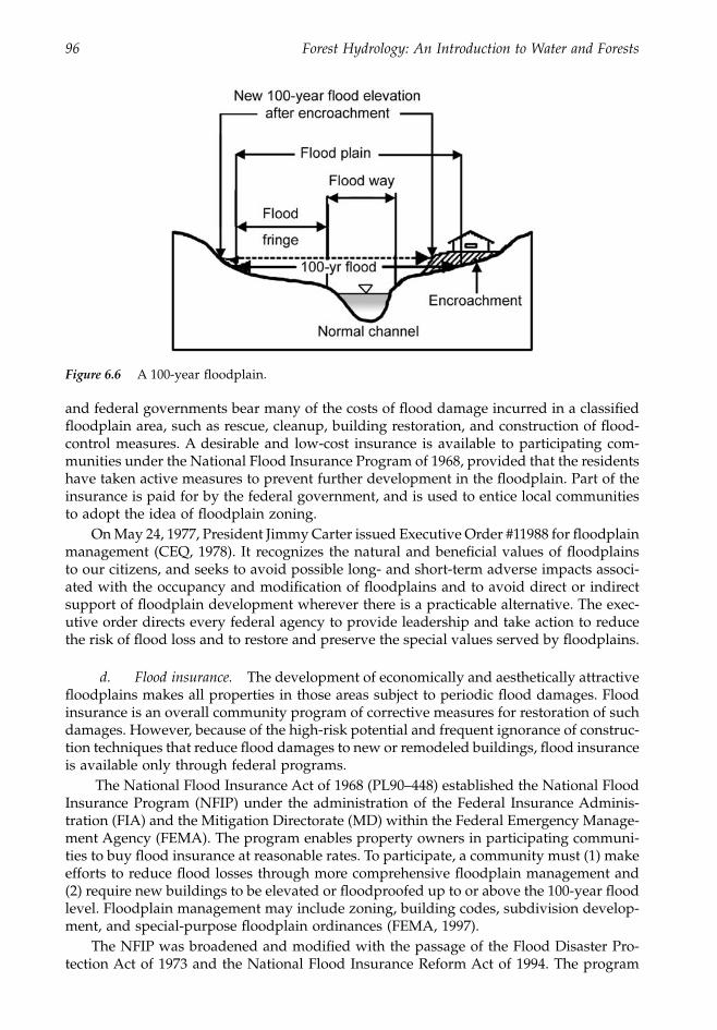
96 Forest Hydrology: An Introduction to Water and Forests
and federal governments bear many of the costs of flood damage incurred in a classifiedfloodplain area, such as rescue, cleanup, building restoration, and construction of flood-control measures. A desirable and low-cost insurance is available to participating com-munities under the National Flood Insurance Program of 1968, provided that the residentshave taken active measures to prevent further development in the floodplain. Part of theinsurance is paid for by the federal government, and is used to entice local communitiesto adopt the idea of floodplain zoning.
On May 24, 1977, President Jimmy Carter issued Executive Order #11988 for floodplainmanagement (CEQ, 1978). It recognizes the natural and beneficial values of floodplainsto our citizens, and seeks to avoid possible long- and short-term adverse impacts associ-ated with the occupancy and modification of floodplains and to avoid direct or indirectsupport of floodplain development wherever there is a practicable alternative. The exec-utive order directs every federal agency to provide leadership and take action to reducethe risk of flood loss and to restore and preserve the special values served by floodplains.
d. Flood insurance. The development of economically and aesthetically attractivefloodplains makes all properties in those areas subject to periodic flood damages. Floodinsurance is an overall community program of corrective measures for restoration of suchdamages. However, because of the high-risk potential and frequent ignorance of construc-tion techniques that reduce flood damages to new or remodeled buildings, flood insuranceis available only through federal programs.
The National Flood Insurance Act of 1968 (PL90–448) established the National FloodInsurance Program (NFIP) under the administration of the Federal Insurance Adminis-tration (FIA) and the Mitigation Directorate (MD) within the Federal Emergency Manage-ment Agency (FEMA). The program enables property owners in participating communi-ties to buy flood insurance at reasonable rates. To participate, a community must (1) makeefforts to reduce flood losses through more comprehensive floodplain management and(2) require new buildings to be elevated or floodproofed up to or above the 100-year floodlevel. Floodplain management may include zoning, building codes, subdivision develop-ment, and special-purpose floodplain ordinances (FEMA, 1997).
The NFIP was broadened and modified with the passage of the Flood Disaster Pro-tection Act of 1973 and the National Flood Insurance Reform Act of 1994. The program
Figure 6.6 A 100-year floodplain.
1363_C06_fm Page 96 Wednesday, December 4, 2002 7:41 AM

Chapter six: Water resource problems 97
enables property owners in participating communities to buy flood insurance at reasonablerates. Commercial insurance companies can sell and service flood insurance in their namesunder the FIA’s Write Your Own (WYO) program. WYO was intended to increase thegeographic distribution of the NFIP policies and to improve service to the policyholders.As of October, 1996, about 90% of insurance companies had signed arrangements withFIA under the WYO program.
Federal flood insurance coverage is available to all owners of insurable property ina community participating in the NFIP. The insurable property refers to a building andits contents that are principally above ground and not entirely over water. Buildingsentirely over water or principally below ground, animals, crops, and all objects in theopen are not insurable.
Flood insurance under the NFIP is not available within communities that do notparticipate in the NFIP. A participating community that does not enforce its floodplainmanagement ordinances can be placed on probation or suspended from the program. Theprobation may last up to 1 year, and an additional $50 charge is added to the premiumfor each policy for at least 1 year after the probation period begins.
e. Disaster aids. The federal government also provides assistance programs thatcompensate disaster victims for economic damages suffered from flooding. FEMA coor-dinates most of the direct assistance to nonagricultural losses while the USDA providesdirect compensation for damages to crops. Both programs are available only in countieswhere the President has declared a disaster.
FEMA administers the Hazard Mitigation Grant Program for compensation of dam-ages to local governments and the Individual and Family Assistance Program for directaid in temporary housing, counseling, and property loss to flood victims. FEMA distrib-uted over $5 billion in direct assistance to presidentially declared disaster areas between1965 and 1989 and $27.6 billion between 1989 and 1993.
The USDA provides two programs to compensate for crop damages: the Federal CropInsurance Program and Agricultural Disaster Assistance. The Federal Crop InsuranceProgram is implemented through designated insurance companies and covers 51 cropsincluding wheat, cotton, sorghum, barley, corn, and rice. Farmers pay premiums up frontand get compensation when crop losses are incurred. The Agricultural Disaster Assistanceprogram is a noninsured assistance program that applies only to presidentially declareddisaster areas. If qualified, each individual can get assistance up to 60% of total losses or$50,000.
The declaration of a disaster starts at the county level. A county committee gathersdata on weather, crops, and production to support the disaster conditions. The data arethen sent to a committee at the state level. The state committee, after reviewing recom-mendations from local committees, will determine the disaster areas and request a decla-ration from Washington, D.C. Once an area is declared a disaster by the President, thelocal government and residents are qualified to apply for assistance from USDA or FEMA.
III. Water qualityDue to its solubility and its role as a habitat for aquatic life, all water in nature containsorganic matter, inorganic matter, and dissolved gases derived from its environment, fromman’s activities, from the atmosphere, or from living organisms. The concentration ofthese substances and the biological, physical, and chemical effects of these substances arethe basic criteria in the determination of water quality. In practice, water is consideredpolluted if it is not suitable for intended uses such as drinking, recreation, irrigation,
1363_C06_fm Page 97 Wednesday, December 4, 2002 7:41 AM
98 Forest Hydrology: An Introduction to Water and Forests
industry, or aquatic life. The U.S. EPA (1976; 1998) has established national water qualitystandards for various uses.
Water pollution is probably the most common hazard to people in much of the world.About 20% of the world’s population lacks access to safe drinking water, and about 50%lacks adequate sanitation (UNEP, 1999). In the U.S., the EPA indicated that 95% of the 246hydrologic drainage basins in the U.S. were affected by water pollution in 1977 (CEQ,1978). Under Section 305(b) of the Clean Water Act, the states assessed water-qualityconditions of 17% of total river-miles, 42% of total lake-acres, and 78% of estuarine watersin 1994. The results showed that 64% of river miles, 63% of lake acres, and 63% of estuarinewaters assessed were found to fully support uses designated for them (Bucks, 1997). Thiswas a great improvement in the 20-year period. However, about 60% of the impairmentsin rivers and 50% in lakes came from agriculture. Groundwater is generally assumed safeand pollution free, counting on the filtering effect of Earth on moving water. However,some groundwater aquifers are occasionally contaminated due to intrusion of seawater,sewer leakage, waste discharged to the ground, and other contaminants.
Polluted water affects human health and aquatic life, and it compounds the problemsof water scarcity. It affects the health of about 120 million people and contributes to thedeath of about 15 million children under the age of five every year (WMO, 1992).
A. Water pollutants
All substances that make water unsuitable for intended uses are water pollutants. Theycan be classified into eight categories.
1. SedimentsStream sediments are soil and mineral particles, usually inorganic, but in part organic orcomposites of the two, released from the land by surface runoff, streamflow, wind, meltingglaciers, raindrop impact, animals, gravity, or avalanche. The amount of sediment deliv-ered to waters in the U.S. each year exceeded 4 ¥ 109 t in the 1960s, a quantity greaterthan the total sewage load by 500 to 700 times (Glymph and Carlson, 1966). Today, it isstill the largest single water pollutant in the nation (EPA, 1997).
Physically, the presence of sediment can affect water turbidity, light penetration,energy exchange, taste, odor, temperature, and abrasiveness. When deposited, it candeplete reservoir capacity, clog stream channels and drainage ditches, alter aquatic habitat,suffocate fish eggs and bottom-dwelling organisms, form alluvium, and increase floodingand flood damages. Also, excessive siltation interferes with drinking-water–treatmentprocesses and recreational use of rivers. Chemically, many plant nutrients, mineral ele-ments, organic chemicals, fertilizers, insecticides, herbicides, and radioactive substancescan attach to the soil particles to be carried to streams with sediment. These substancesare responsible for degradation of water quality, lake eutrophication, and harmful effectson aquatic life and human health. Biologically, aquatic ecosystems can be affected directlyby the physical presence of sediment or indirectly by the interaction of sediment with thephysical and chemical environment of the stream.
2. HeatExcessive heat caused by the summer sun, the reduction of flow volume, the removal ofriparian plants, and the discharge of heated water from power plants and other industriescan be a serious pollution problem. Higher water temperature causes lower viscosity,greater sediment-falling velocity, increased chemical reaction, reduction in dissolved oxy-gen, and more evaporation. Biologically, the undesirable blue-green algae and otherdestructive microorganisms can be reproduced or introduced in warm water due to their
1363_C06_fm Page 98 Wednesday, December 4, 2002 7:41 AM
Chapter six: Water resource problems 99
tolerance of higher temperature. Not only are blue-green algae undesirable as aquaticanimal food, they also give off toxic substances and cause a series of problems in waterquality. A change in water temperature by a few degrees can adversely affect the survival,migration, spawning, and reproduction of fish.
3. Oxygen-demanding wastesOxygen-demanding wastes include domestic sewage, animal manure, and some industrialwastes of largely carbonaceous organic material that can be decomposed by microorgan-isms to carbon dioxide, water, some basic ions (such as ), and energy. Thedecomposition of organic material in water is carried out by bacteria at the expense ofdissolved oxygen. Since the maximum level of dissolved oxygen in water is about 15mg/liter the activity of bacteria can deplete oxygen concentration. This can cause detri-mental effects to other aquatic organisms if sufficient organic matter and other conditionsare favorable for multiple expansion and bacteria activity. Large amounts of sewage orother oxygen-demanding wastes from industry or agriculture can deplete the dissolvedoxygen level in the water to septic conditions.
A common parameter to describe the oxygen demand of waste is the 5-day biochem-ical oxygen demand (BOD). It measures the rate at which oxygen is used rather than thelevel of oxygen in the water or in certain specific pollutants. A very low value of BODimplies either that the water is clean or that the bacteria are inactive. In either case, thedissolved oxygen level is usually high.
4. Plant nutrientsFrequently, plant nutrients such as nitrogen and phosphorus are added to reservoirs bydissolving in runoff water or attaching to eroding soil particles. Nutrients may come from(1) soil and water erosion, (2) agricultural fertilizers, (3) domestic sewage, (4) livestockwastes, (5) decomposition of plant residuals, and (6) phosphate detergents. They stimulatethe growth of aquatic plants, which in turn interfere with water use, produce disgustingodors when they decay, and add BOD to the water. Waters excessively enriched withnutrients are referred to as eutrophic. They have high plant populations and appear turbidand greenish in color. As a result, algae and aquatic weeds bloom excessively, destroyaesthetic qualities, and interfere with fishing, sports, navigation, irrigation, and the gen-eration of hydroelectric power.
5. Disease-causing agentsWaste discharges from cities, slaughtering plants, animal feedlots, or ships can carrybacteria, viruses, or other microorganisms capable of producing disease in man andanimals. These microorganisms are responsible for such diseases as cholera, typhoid fever,dysentery, polio, and infectious hepatitis. However, waters contain numerous kinds ofpathogenic bacteria, and identification of each one is both time consuming and expensivefor routine pollution tests. Coliform bacteria are relatively harmless microorganisms thatlive in the gut of animals and are discharged with feces in sewage-contaminated waters.Their existence and density are reliable indicators of the adequacy of treatment for thereduction of pathogens in water. Thus, the most probable number of coliform bacteria inwater samples becomes a standard parameter for the determination of pathogenic pollu-tion. A high count of coliform indicates the probability of the presence of a high numberof disease-causing microorganisms in the water. The maximum for drinking water is 1 per100 ml, and 200 per 100 ml for swimming.
NO3–, PO4
–, SO4–
1363_C06_fm Page 99 Wednesday, December 4, 2002 7:41 AM

100 Forest Hydrology: An Introduction to Water and Forests
6. Inorganic chemicals and mineralsMany acids, salts, heavy metals, and toxic pollutants from industrial and municipal dis-charges affect water quality adversely in more than 70% of the large river basins in theU.S. (CEQ, 1978). Acid mine drainage (AMD) arises from strip-mining and underground-mining areas when iron pyrites (FeS2) are oxidized into ferric hydroxide [Fe(OH)3] andsulfuric acid (H2S04) through water, air, and bacteria. AMD affects a total length of morethan 17,600 km of U.S. streams (ReVelle and ReVelle, 1984). It is characterized by highlyacidic water and stream bottoms coated with ferric hydroxide (yellow color), creating anenvironment toxic to aquatic life.
Mercury, cadmium, arsenic, zinc, and lead are some examples of other inorganicchemicals contaminating rivers and water supplies, toxic to aquatic species and humanhealth. Chlorine has been applied to destroy disease-causing bacteria in drinking water,but it can combine with organic compounds in the water to form chlororganic compoundssuch as chloroform, carbon tetrachloride, and trihalomethanes (THMS). These chemicalshave been found to cause cancer in rats and mice, and may have some effects in people(Owen, 1985). Many different pollutants are present in the stream environment. Thepresence of certain particulate matter can increase the toxicity of other pollutants, afunction usually referred to as potentiation. In other cases the combined effects of two ormore pollutants are more severe or different in quality from each individually, a phenom-enon called synergism. It is called antagonism if the combined effects of two pollutantsare less severe than each individual. All these make the effects of water pollution extremelydifficult to study.
7. Synthetic organic chemicalsDetergents, plastics, oil, pesticides, septic-tank cleaners, phenols, DDT, and many otherorganic compounds are products of modern industrial technology. Some of these chemicalsare slowly degradable pollutants, while the others are nondegradable. The slowly degrad-able chemicals remain in the water for a long period of time but are eventually brokendown to harmless levels by natural processes. Nondegradable pollutants, such as plastics,cannot be broken down in nature and must be controlled either by removing them throughmechanical treatment or by preventing them from entering the environment.
Synthetic organic chemicals can disrupt aquatic ecosystems, damage the economic,recreational, and aesthetic value of lakes and rivers, impair the taste and odor of water,enhance growth of algae and aquatic weeds, and poison fish, shellfish, predatory birds,and mammals. They can be toxic to humans, induce birth and genetic defects, or causecancer. Since many new compounds can be introduced each year without testing of theirenvironmental effects, it is possible that they will have caused chronic damage to humanhealth and to aquatic life long before scientists realize their effects.
8. Radioactive substancesRadioactive substances can come from radioactive rocks and soils, from uranium miningand processing, from nuclear power plants, from nuclear weapon tests, or from leakageof radioactive instruments and laboratories. They can cause chronic effects to humanhealth such as cancer and genetic defects.
B. Sources of water pollution
For management purposes, surface water pollution is generally identified as point sourcesor nonpoint sources. If wastes and pollutants are discharged from identifiable locations,they are point sources of water pollution. Point sources can come from municipal sewage,
1363_C06_fm Page 100 Wednesday, December 4, 2002 7:41 AM
Chapter six: Water resource problems 101
industrial plants, animal feedlots, combined storm runoff and sewer lines, offshore oil-well or tanker accidents, and power plants. Thus, point-source pollution is generallycreated by man’s activities and is discharged into receiving water through “discernible,confined, and discrete conveyances including but not limited to any pipe, ditch, channel,tunnel, conduit, well, discrete fissure, container rolling stock, concentrated animal feedingoperation, or vessel or other floating craft,” as defined by the Federal Water PollutionControl Act Amendments of 1972 (PL 92–500). When discharges from a point source exceedeffluent limitations, the discharges must be treated, treatments must be upgraded, or thedischarges terminated.
If pollutants come from the land surface, their sources are difficult to identify, theirroutes are intermittent and diffused, and their occurrences are associated with storms andsurface runoff, then they are nonpoint sources of water pollution. They include:
Sediment from natural ground surfaces, forest activities, agricultural production, con-struction, mining, grazing
Chemicals from applications of fertilizers, pesticides, herbicides, saline waterirrigation
Urban storm runoffAcids and minerals drained from minesAcid depositionUntraceable oils and other hazardous materials
Generally, nonpoint sources of water pollution cannot be corrected using technologyand treatments similar to those employed for point sources of water pollution. Instead,“best management practices (BMPs)“ to land and vegetation are adopted to all of man’sactivities and to all areas that have potential to generate water pollution. The term BMPis a vague and localized approach, depending on soil, topography, vegetation, and climatesof the area. Using mulches alone to reduce soil erosion may be a good BMP in locationA, but might not be effective enough in location B.
Ground water can be contaminated with organic chemicals through a number of pointand nonpoint sources. They include waste lagoons; groundwater recharge activities; leaksfrom sewers, septic tanks, or gasoline-storage tanks; injection wells of waste disposal andoil fields; drainage from landfill and mining operations; seawater intrusion; chemicalsapplied to soils; and pumping wells.
C. Water quality control
Controlling water quality is a tedious and complicated process. It involves scientificresearch, technological development, resources management, economic analysis, polit-ical movements, law enforcement, public participation, and education. An effectivewater-quality program requires technical and financial assistance from governments,cooperation and support from industries and farmers, and awareness and participationfrom the public.
In dealing with water-quality problems, one should keep in mind that prevention ischeaper than reclamation and that the nation’s pollutants from nonpoint sources are muchgreater than those from point sources. Thus, protection and prevention of streams withgood water quality from deterioration should be the first consideration. Proper andimproving land management is an important element in the nation’s water-quality pro-grams. Control of water-quality programs includes the following tasks.
1363_C06_fm Page 101 Wednesday, December 4, 2002 7:41 AM

102 Forest Hydrology: An Introduction to Water and Forests
1. Monitoring and researchThe environmental effects of pollutants and their tolerance levels for various uses needto be studied. The basic knowledge for each pollutant in the aquatic environment such asits biological magnification; the residence time in soil, air, water, plants, animals, andpeople; any synergistic interaction with other pollutants; and any adverse effects onecosystems, aquatic life, physical environment, and human health all need to be fullyunderstood. The tolerance level of each pollutant needs to be determined and water-quality standards for various uses need to be established.
Monitoring is basic to research and management. Water-quality levels and sources ofpollutants need to be continuously monitored at local, regional, national, and global levels.Pollution sources need to be identified. The long-term water-quality conditions fromundisturbed forested areas can serve as an important basis for aquatic water-qualitystandards for the region. In addition to these chemical and physical measurements, eco-logical and biological changes in our ecosystems need to be measured. The ecologicalmeasurements should be evaluated with respect to short- and long-range effects of waterpollution.
2. Public educationAwareness on the part of the general public of water-pollution problems is an importantelement of water-pollution–control programs. It can be accomplished through publicschools, TV programs, workshops, and town meetings.
3. Prevention and treatmentNonpoint sources of water pollution can be greatly reduced by preventing pollutants,mainly sediment and nutrients, from running off to creeks by application of the “bestmanagement practices.” Point sources of water pollution, such as industries and cities,can be prevented first by use of “best practical technology” and later by improved “bestavailable technology.” Land management practices such as mulching, terracing, contourcropping, strip cropping, and planting cover crops greatly increase soil infiltration, reduceoverland runoff, and consequently cut down sediment delivered to the streams. Tradi-tionally, the effluent from paper and pulp plants impairs the water quality of streams, buta new technique using a dry-barking process removes bark from poplar and aspen treeswithout water, and consequently there is no discharge of pollutants to streams (Owen,1985). Many industries have developed effective technology either to reduce the amountof discharged wastes or to convert their wastes into commercially valuable by-products.
Polluted water can undergo various levels of purification and treatment, dependingon the sophistication of the plant and the degree of purity desired. Treatment of liquidwastes may involve mechanical (primary), biological (secondary), and specialized chem-ical and physical (tertiary) processes. Disinfection is also carried out in final stages ofsewage treatment to remove water coloration and to kill bacteria and viruses.
4. ManagementStandards for the design, construction, operation, and maintenance of sewer systems andtreatment plants need to be established. State and federal governments may need toprovide financial assistance to municipalities in water-pollution–abatement programs. Itis also important to develop different water-quality standards for various uses. Institu-tional activities of water-pollution control among governments at different levels andbetween countries need to be coordinated properly. National water-pollution policies needto be established as guidelines for controlling various programs.
1363_C06_fm Page 102 Wednesday, December 4, 2002 7:41 AM
Chapter six: Water resource problems 103
5. Legislation and enforcementPolicies and regulations on water quality need to be established legislatively at the federal,state, and local levels. Legislatures provide authorities, standards, finance, guidelines,responsibilities, and assessment for control and management programs on water quality.Industries and individuals are fined or penalized if they do not comply with environmentallaws and regulations. Severe violations of such laws can cost them their operating licenses,and companies may even be shut down through legal action.
D. Water-quality laws and regulations
Two laws are of paramount importance in control of water quality conditions in the U.S.One is the Rivers and Harbors Act of 1899, and the other is the Clean Water Act of 1977.The 1899 Act flatly prohibits discharging refuse matter of any kind from a ship or shoreinstallation into navigable waters in the U.S. Depositing material of any kind in any placeon the bank of any navigable waters that can be washed off into the waters is alsoprohibited. The U.S. Army Corps of Engineers was authorized to require permits beforeanything can be dumped, deposited, or constructed in any navigable U.S. waterway.
The Clean Water Act (CWA), formally known as the Federal Water Pollution ControlAct Amendments of 1972 (PL 92–500) and originally enacted in 1948 (PL 80–845), is theprincipal law governing pollution in the nation’s streams, lakes, and estuaries. It set anambitious interim goal of making all U.S. waters safe for fish, shellfish, wildlife, and peopleby 1983 and a national goal of eliminating all discharges into U.S. waters by 1985. TheEPA, the federal agency charged with the programmatic responsibilities for the nation’senvironmental quality, was required by PL92–500 to establish a system of national effluentstandards. Each state was required to establish regulations for nonpoint sources of waterpollution (Section 208). The Army Corps of Engineers was authorized to regulate thedischarge of dredged and fill material into navigable waters (Section 404). Both point andnonpoint sources were considered a threat to the nation’s water-quality conditions andwere controlled simultaneously.
Congress made certain important amendments in 1977 (PL 95–217), 1981 (PL 97–117),and 1987 (PL 100–4). A new section (319) entitled “Nonpoint Source Management Pro-grams” to improve Section 208 “Nonpoint Source Planning Process” was added to the1987 law. In addition to the existing industrial and municipal stormwater-discharge pro-grams known as the National Pollutant Discharge Elimination System (NPDES), it alsoestablished a program for controlling toxic-pollutant discharges. Overall, the law is acomprehensive and complex water-quality–management law; it establishes water-qualitypolicies, regulations, permits, requirements, and deadlines on water-quality standards,quality assessments, reduction of discharges from point and nonpoint sources, water-quality certification, enforcement, financial assistance, and nationwide corporations.
Five primary provisions of the law have impacts on forestry and other related natural-resources activities. They are Sections 208 (nonpoint pollution planning), 303 (total max-imum daily load, TMDL), 304 (water quality standards), 319 (water pollution assessmentand management programs), and 404 (wetlands and dredging activities). Traditionally,nonpoint sources of water pollution are managed through the two nonregulatory Sections208 and 319. Recent developments show that the TMDL process is becoming a powerfultool to control point and nonpoint sources of activities (Dubensky and Ice, 1997).
IV. Water rightsIncreasing competition and conflicting interests in water make water rights a legal, andsometimes a political, problem in water resources. The problem is triggered by the facts
1363_C06_fm Page 103 Wednesday, December 4, 2002 7:41 AM
104 Forest Hydrology: An Introduction to Water and Forests
that (1) water is necessary for survival and development, (2) there is not always enoughwater of the right quality in the right place at the right time, and (3) water in a river isoften shared by many countries and by users of different withdrawal intensities. Forexample, the same stream may be needed by farmers in upper reaches, by manufacturersor recreationalists in middle reaches, by city planners downstream, and by fishermen inthe bay estuaries. An absence of clearly defined water rights and rules of liability cancause hateful actions among individuals and communities or between nations.
The fact that water is a moving, returnable, and critical resource with various tangibleand intangible values makes water allocation necessarily different from the traditionalconcepts of private ownership. Absolute ownership may not be appropriate. All allocationsamong uses and users should be considered in terms of survivability, productivity, envi-ronmental integrity, and fairness.
Generally, waters on Earth can be grouped into five distinct categories in accordancewith their geographical locations: atmospheric, ocean, diffused, surface, and groundwater.No legal rights have yet been established with respect to uses of clouds for artificial rain.It might become a problem, however, as cloud-seeding techniques advance to greatereffectiveness. Ocean water is generally regarded as a universal commodity. It can be usedin navigation, fishing, recreation, and other purposes subject to national and internationallaws. The diffused, surface, and groundwater rights are of great concern to watershedmanagement.
A. Diffused water
Water on the ground surface not in connection with a stream channel is considered diffusedwater. Diffused waters include bogs, fallen rain, fallen snow, springs, seepage, waterdetached from subsiding floods not forming a part of a water course or lake, and anywater that has not yet reached a recognized water course, lake, or pond. Thus, springsthat run directly into a stream are not considered diffused water.
Diffused water is generally regarded as the property of the landowner. It allowslandowners an absolute right to any use of diffused waters on their lands, includingdamming, storing, selling, or even preventing it from flowing to adjoining lands. Theunlimited right to capture diffused water may affect downstream water flow and ground-water level, especially in arid and semiarid regions. Because virtually no states attemptto regulate landowner uses of diffused water, no legal action can be taken to stop thiscapture.
B. Surface water
A body of water flowing in a well-defined channel or watercourse is regarded as surfacewater. It is the water that is found in lakes, ponds, rivers, creeks, streams, and springs.Water contained in a surface depression as a result of rainfall or snowmelt is generallynot considered surface water. Allocations for surface water are generally guided by threedoctrines of water law: riparian, prior appropriation (or Colorado), and hybrid (orCalifornia).
1. Riparian rights. Lands bordering a watercourse give the landowners specialrights to make use of water in the channel, provided such use is reasonable relative to allother users. These rights include domestic and household uses, and water for livestock,navigation, power generation, fishing, recreation, and other purposes. Generally the land-owner has no right to use water if his land does not adjoin a stream course. If there isinsufficient water to satisfy all reasonable riparian needs, then uses of water must be
1363_C06_fm Page 104 Wednesday, December 4, 2002 7:41 AM
Chapter six: Water resource problems 105
reduced in proportion to the land size. The doctrine of riparian right is applied mainly inthe eastern half of the U.S.
2 Prior appropriation. The riparian-rights doctrine is inadequate in the arid West,where water is generally scarce and less dependable than in the humid East. Under theprior-appropriation doctrine, both riparian and nonriparian owners have specific rightsto divert water from streams or other bodies of water as long as their use does not conflictwith prior claims. The theme of water rights is first-come, first-served with prioritydetermined by a recording system similar to that used for land transactions. Thus, waterrights depend on usage, not land ownership. Prior appropriation gives an exclusive rightto the first appropriator. The rights of later ones are conditioned by the prior rights ofthose who have proceeded. However all rights are conditioned upon beneficial use as aprotection to later appropriators against the wasteful use by those with earlier rights. Theappropriation rules are exercised in nine Western states: Alaska, Arizona, Colorado, Mon-tana, New Mexico, Utah, and Wyoming.
3 Hybrid doctrine. Ten other states — California, Kansas, Mississippi, Nebraska,North Dakota, Oklahoma, Oregon, South Dakota, Texas, and Washington—adopt a portionof the riparian and the prior-appropriation doctrines. In general, this modified doctrinerestricts the rights of the riparian owner while recognizing appropriation rights to reason-able amounts of water used for beneficial purposes. The limitations of riparian rightsinclude: (1) reasonable use and (2) elimination of unused riparian rights by statute. Thus,a riparian cannot prevent an appropriation to a nonriparian unless interference with theriparian’s reasonable use of water can be proven.
4. Reserved-rights doctrine. The U.S. is entitled to claim water rights for instreamflows on federal lands or in Indian reservations. In March, 1891, Congress passed theForest Reserve Act (or Creative Act) allowing the President of the U.S. to set aside forestreserves, whether of commercial value or not, to be inaccessible to the public for anypurpose. The forest reserves were further specified under the Organic Act of 1897 toprovide a continuous supply of timber and secure favorable conditions of water flow. Inthe 1963 Arizona vs. California case, the court ruled that a sufficient reserve of water isaccompanied with the U.S. lands when they were reserved for a particular purpose(Gordon, 1995). Under this doctrine, lands such as national forests, national parks, nationalwildlife refuges, and the wild and scenic rivers that are reserved from the public domainfor a particular purpose may be claimed for water rights to carry out that purpose (Lamband Doerksen, 1990). Thus, reserved water rights on federal lands do not exist by statute.They are required to be identified and quantified by court procedures.
In another case, the Colorado Supreme Court concluded in 1987 that the federalgovernment could claim water rights based on the Organic Act, and that each claim mustbe properly examined or determined for its: (1) documents reserving the land from thepublic domain and the Organic Act, (2) precise purposes, (3) importance of water for suchpurposes, and (4) precise quantity of water required.
On the basis of the Organic Act, the Department of Justice, representing the ForestService and acting on behalf of the U.S., filed claims for federal reserved water rights in1976 to keep certain amounts of water for the Arapahoe, Pike, Roosevelt, and San IsabelNational Forests within Water Division 1 in Colorado to protect stream channels andtimber. These claimed water rights were for three purposes: (1) fire fighting, unlimitedamount, (2) administrative sites, not more than 10 acre-ft (12,335 m3)per site per year andnot more than one site per 100,000 acres (40, 470 ha) of national forest, and (3) instreamflows for channel maintenance, 50% of average annual runoff.
1363_C06_fm Page 105 Wednesday, December 4, 2002 7:41 AM
106 Forest Hydrology: An Introduction to Water and Forests
However, these claims were challenged by the State of Colorado and Water Conser-vancy districts in northern Colorado that divert water from national forests. The oppositionclaimed that the U.S. did not need water rights because it had other mechanisms forcontrolling diversions such as special-use permit, and that such claims of water rightswould injure other water users, especially during the critical spring runoff period.
The case went to trial in 1990 in District Court, Water Division 1, of the State ofColorado. Closing arguments were made in March 1992 and the court decision and orderwere on February 12, 1993. The judge recognized the reserved water rights of the U.S.,but the applicant (U.S.) failed to show that the claims were necessary to preserve thetimber or to secure favorable water flows, and failed to establish the minimum quantityneeded to ensure that purpose. Thus, the court granted water rights for fire-fighting andadministrative sites to the U.S. and suggested the Forest Service use its special-use per-mitting authority to control water diversion in lieu of obtaining water rights on instreamflows (Gordon, 1995).
C. Groundwater
Either flowing water in an underground channel (aquifer) or diffused percolating wateris considered groundwater. Allocating rights and obligations in groundwater among thestates is based either on the concept of property ownership or on the notion of a sharedpublic resource, or both (Getches, 1984). Thus, a state may (1) recognize the ownershipof groundwater by the overlying landowner, (2) limit the use of groundwater at a rea-sonable level, (3) provide a special protection for prior users, or (4) manage groundwaterresources as public property with rights created under a permit program. Groundwateris a part of the hydrological system. Any pumping activities at one site would affect thewater table and water yield in nearby locations. Thus, absolute ownership and uncon-trolled use of groundwater is no longer feasible. Many states adopted the concepts ofreasonable use and correlative rights to protect all landowners against the inadvertentactivities of a few others.
ReferencesAnderson, H.W., Hoover, M.D., and Reinhart, K.G., 1976, Forest and Water: Effects of Forest Man-
agement on Floods, Sedimentation, and Water Supply, General Tech. Rep. PSW-18, U.S. ForestService, Pacific Southwest Forest and Range Exp. Sta.,
Baumgarter, A., and Reichel, E., 1975, The World Water Balance, Mean Annual Global, Continental andMaritime Precipitation, Evaporation, and Runoff, R. Oldenbourg, Munich.
Borrell, J., 1986, A plan to make the desert gush, Time, September 29, 1986.Bucks, D.A., 1997, Competition for water use — an agricultural perspective, Environ. Prof., 19, 33–34.California Department of Water Resources, 1973, The California Water Plan, Sacramento, CA.Carter, V. et al., 1978, Water resources and wetlands, in Wetland Functions and Values: The State of
Our Understanding, Am. Water Resour. Assoc, pp. 344–375.CEQ, 1978, Environmental Quality, The 9th Annual Rep., Council on Environmental Quality, Govern-
ment Printing Office, Washington, D.C. Chang, M. and Watters, S.P., 1984, Forests and other factors associated with streamflows in east
Texas, Water Resour. Bull., 20, 713–720.Clark, C.,1982, Flood, Time-Life Books, Alexandria, VA. Clean Water Act, 1977, 33 USC (United States
Code) 1251, H.R. 3199.Dregne, H.E., 1983, Desertification of Arid Lands, Hardwood Academic Publishers, New York.Dubensky, M. and Ice, G., 1997, Common issues and challenges in Clean Water Act programs —
natural resource policy and research perspectives, Environ. Prof., 19, 58–61.EPA, 1976, Quality Criteria for Water, Government Printing Office, Washington, D.C.
1363_C06_fm Page 106 Wednesday, December 4, 2002 7:41 AM

Chapter six: Water resource problems 107
EPA, 1997, Monitoring Guidance For Determining the Effectiveness of Nonpoint Source Controls,EPA 841-B-96–004, U.S. Environmental Protection Agency.
EPA, 1998, Current Drinking Water Standards, Office of Ground Water and Drinking Water,www. epa.gov/OGWDW/wot/appa.html.
Federal Water Pollution Control Act Amendments, 1972, 33 USC (United States Code), 1151, 70 stat.498, 84 stat 91, S.2770.
FEMA, 1997, Answers to Questions about the National Flood Insurance Program, Federal EmergencyManagement Agency, Washington, D.C.
Getches, D.H., 1984, Water Law, West Publishing, St. Paul, MN.Gleick, P.H., 1998, The World’s Water, Island Press, Washington, D.C.Gleick, P.H., 2000, The World’s Water, 2000–2001, Island Press, Washington, D.C.Glymph, L.M. and Carlson, C.M., 1966, Cleaning up Our Rivers and Lakes, Am. Soc. Agr. Eng.,
Paper No. pp. 66–74, St. Joseph, MI.Goodman, J., 1985, The collection of fog drip, Water Resour. Res., 21, 392–394.Gordon, N., 1995, Summary of Technical Testimony in the Colorado Water Division 1 Trial, General
Tech. Rep. RM-GTR-270, U.S. Forest Service, Rocky Mountain Forest and Range ExperimentStation.
Harr, R.D., 1982, Fog drip in the Bull Run municipal Watershed, Oregon., Water Resour. Bull., 18,785–789.
Husseiny, A.A., Ed., 1978, Iceberg Utilization, Pergamon Press, Elmsford, NY.Ingwersen, J.B., 1985, Fog drip, water yield, and timber harvesting in the Bull Run municipal
watershed, Oregon, Water Resour. Bull., 21, 469–473.Jordaan, J. et al., 1993, Water in our common future, a research agenda for sustainable development
of water resources, UNESCO International Hydrological Programme, Paris. Lamb, B.L. and Doerksen, H.R., 1990. Stream water use in the United States — water laws and
methods for determining flow requirements, in National Water Summary 1987 — HydrologicEvents and Water Supply and Use, Water Supply Paper 2350, U.S. Geological Survey, pp.109–116.
Maddox, R.A. and Chappel, C.F., 1979, Flash flood defenses, Water Spectrum, 11, 1–8.Mather, J.R., 1984, Water Resources: Distribution, Use, and Management, John Wiley & Sons, New York.MIT, 1971, Inadvertent Climate Modification, Rep. of the Study of Man’s Impact on Climate (SMIC),
Massachusetts Institute of Technology. Murray, C.R., 1968, Estimated use of water in the United States, 1965, U. S. Geological Survey Circular
556, Washington, D.C.National Water Commission, 1973, Water Polices for the Future, Government Printing Office, Wash-
ington, D.C.Novitzki, R.P., 1978, Hydrologic characteristics of Wisconsin’s wetlands and their influences on
floods, streamflow, and sediment, in Wetland Functions and Values: The State of Our Under-standing, Am. Water Resour. Assoc., pp. 377–88.
Ooura, H., 1952, The capture of fog particles by the forest, J. Meteo. Res., Suppl., pp. 239–259.Owen, O.S., 1985, Natural Resources Conservation, 4th ed., MacMillan, New York.ReVelle, P. and ReVelle, C., 1984, The Environment, Issues and Choices for Society, Willard Grant Press,
Boston.Rivers and Harbors Act, 1899, 33 USC (United States Code) 401–413.Robinson, D.F., Ed., 1988, Living on the Earth, National Geographical Society, Washington, D.C.Sharpe, W.E., 2001, personal communication, Pennsylvania State University, University Park, PA.Shaw, E.M., 1983, Hydrology in Practice, Van Nostrand Reinhold, New York.Skillings, T.E., 1999, Water reuse: the wave of the future, in Watershed Management to Protect Declining
Species, Proc., AWRA, December 1999, pp. 481–484.Solley, W.B., Pierce, R.R., and Perlman, H.A., 1998, Estimated Use of Water in the United States in
1995, U.S. Geological Survey Circular 1200, Washington, D.C. Stulp, J.R., 1995, Social, political, and educational factors involved in facilitating municipal waste
utilization, in Agriculture Utilization of Urban and Industrial By-Products, Karlen, D.L., et al,Eds., Am. Soc. Agron. Spec. Publ. No. 58, pp. 1–10.
Texas Water Development Board, 1994, “Forty-nine water saving tips,” Austin, TX.
1363_C06_fm Page 107 Wednesday, December 4, 2002 7:41 AM

108 Forest Hydrology: An Introduction to Water and Forests
Texas Water Development Board, 1968, The Texas Water Plan, Austin, TX.UNEP, 1999, Global Environment Outlook — 2000, United Nations Environment Programme,
Nairobi, Kenya.UNESCO, 1993, Water for the Common Future, International Hydro. Prog., Committee on Water
Res., Paris.United Nations Environment Programme, 1983, Rain and Stormwater Harvesting in Rural Areas,
Tycooly International, Dublin, Ireland.U.S. Forest Service, 1989, RPA Assessment of the Forest and Rangeland Situation in the United
States, 1989, USDA Forest Service Forest Resource Rep. No. 26, Washington, D.C. U.S. Water News, 1994, Chilean fog collection system furnishes daily baths, U.S. Water News, 11, 2U.S. Water Resources Council, 1968, The Nation’s Water Resources, Part 1, First National Water
Assessment, Washington, D.C.U.S. Water Resources Council, 1978, The Nation’s Water Resources 1975–2000, Vol. 1: Summary; Second
National Water Assessment, Washington, D.C.U.S. Weather Bureau, 1959, Evaporation Maps for the United States, Tech. Paper No. 37, U.S. Dept.
of Commerce.WMO, 1992, International Conference on Water and the Environment: Development Issues for the
21st Century, 26–31 Jan 1992, Dublin, Ireland.WMO/UNESCO, 1991, Water Resources Assessment, WMO/UNESCO report on Progress in the
implementation of the Mar del Plata action and a strategy for the 1990s.Wollman, N. and Bonem, G.E., 1971, The Outlook for Water Quality, Quantity and National Growth,
Johns Hopkins Press University, Baltimore.World Resources Institute, the United Nations Environment Programme, the United Nations
Development Programme, and the World Bank, 1996, World Resources, 1996–97, Oxford Uni-versity Press, Oxford.
Young, C.E., Kinsley, K.R., and Sharpe, W.E., 1983, Impact on residential water consumption of anincreasing rate structure, Water Resour. Bull., 19, 81–86.
Young, E.S. and Sharpe, W.E., 1989, Rainwater Cisterns — Design, Construction, and WaterTreatment, College of Agriculture, Special Circular 277, Penn State University, UniversityPark, PA.
1363_C06_fm Page 108 Wednesday, December 4, 2002 7:41 AM

109
chapter seven
Characteristic forests
Contents
I. A natural resource...........................................................................................................110A. Characteristics .........................................................................................................110B. Forest trees ...............................................................................................................111
1. Canopies .............................................................................................................1112. Root systems......................................................................................................1133. Stems...................................................................................................................114
C. Forest distribution ..................................................................................................1151. Horizontal distribution ....................................................................................116
a. Tropical forests ............................................................................................116b. Temperate forests ........................................................................................116c. Boreal Forests...............................................................................................117
2. Vertical distribution..........................................................................................1173. Forest areas ........................................................................................................118
II. Environmental functions................................................................................................119A. Hydrological ............................................................................................................120B. Climatological..........................................................................................................120C. Mechanical ...............................................................................................................121D. Biological ..................................................................................................................122E. Societal ......................................................................................................................123
III. Functional forests ............................................................................................................123A. Production forests ...................................................................................................123B. Protection forests.....................................................................................................124C. Preservation forests ................................................................................................125D. Public forests ...........................................................................................................126
IV. Threats to forests .............................................................................................................126A. Deforestation and grazing.....................................................................................126B. Forest fires................................................................................................................127C. Air pollution ............................................................................................................127
References .....................................................................................................................................128
Forests have appeared on Earth for 350 million years and reached a peak about 270 millionto 220 million years ago during the Carboniferous period (Burch et al., 1976). Today, forestscover about one third of the Earth’s land surface. They are the most distinguished typeof vegetation community and provide many resources and environmental functions that
1363_C07_fm Page 109 Wednesday, December 4, 2002 7:41 AM
110 Forest Hydrology: An Introduction to Water and Forests
far exceed those of other vegetation covers. Accordingly, forests have always played avital role in the survival, development, and growth of human society since prehistorictimes. Maintaining healthy forests helps improve environmental quality.
I. A natural resource
A forest is a community of somewhat dense growth of vegetation, dominated by treesand other woody plants, that supports an array of microbes and wildlife and occupiesan area large enough to have a distinguished microclimate. Thus, forests are composednot only of many large trees but also of smaller plants with multiple canopy levels, andare home to many animals and other living organisms. They include land, streams, andclimate in a shared and dynamic ecological system. Each forest is uniquely different fromothers because of differences in species composition, age, soils, wildlife, and microclimaticconditions.
There are no clear boundaries on how small an area can be called a “forest.” An areaof plant community, which is not large enough or dense enough to create an environmentand microclimate significantly different from the surrounding areas, probably should beconsidered woodland rather than a forest. If the trees in a stand are artificially regeneratedand professionally cultivated for economic gains, they are called a plantation. The Foodand Agriculture Organization of the United Nations terms forest all lands with trees of7 m or taller and a minimum crown cover of 10% in developing countries or 20% indeveloped regions.
A. Characteristics
Being a natural resource, forests possess a few important characteristics. First, naturalresources are generally divided into either renewable or nonrenewable, depending onwhether or not their uses can be carried on indefinitely. A nonrenewable resource, likecoal and minerals, will be depleted in time if used continuously. If used properly, forestsact like a renewable resource, such as water and solar energy, which cannot be exhausted.However, some types of use can destroy the original forest environment and exhaust theforest and its associated resources. In this case, forests behave like a nonrenewableresource.
For example, many nutrients in tropical rain forests are stored in the biomass abovethe ground and recycled directly between litter and plants. There, soils are fully weathered,rich in iron and aluminum oxides; most nutrients are retained in the organic layers. Thehigh productivity in tropical forests is due to high temperature, long growing season, andrapid recycling of the nutrients, not to the nutrient levels in the mineral soils. Thus, forestclearcutting causes rapid decomposition of the organic matter and extensive leaching ofnutrients, particularly the common cations K, Ca, and Mg, and the organic phosphatereserves (Medina and Cuevas, 1997). As a result, the clearcut sites may take centuries, ormay never be able, to regenerate a forest similar to the original, and loss or even extinctionof many plants from the forest occurs.
Accordingly, forests are in a position between renewable and nonrenewable naturalresources, depending on how well they are treated. They can be classified as “potentiallyrenewable” resources (Mather, 1990), resources that cannot be taken for granted. Abusiveuse of forest resources has resulted in the degradation of the environment, the conversionof fields into deserts, and the disappearance of civilizations.
Second, a forest not only produces wood, fibers, foods, fuels, and medicinal materials;it also provides an environment that affects soil, wildlife, water, and atmosphere. Thus,forest resources should not be referred to as timber resources only. Soil, water, wildlife,
1363_C07_fm Page 110 Wednesday, December 4, 2002 7:41 AM
Chapter seven: Characteristic forests 111
fish, livestock, and recreation resources are all associated with the forest. Without the forestor if the forest is improperly used, all the associated resources will be degraded, damaged,or destroyed.
Third, the forest is considered a “common property” in that any forest activities haveon-site as well as off-site effects. In other words, the effects can expand from the activityforest (site-scale) to adjacent areas (local-scale), distance areas (regional-scale), and remoteareas (global-scale), depending on the areal coverage and intensity of the activity, weatherconditions, and the general circulation of the atmosphere. In Indonesia, the forest fires ofsummer 1997 covered over 1 million hectares of forests, causing haze and smoke inSingapore, Malaysia, Brunei, and the surrounding region for weeks. They released anestimated 220 million to 290 million tons of CO
2
to the atmosphere, about half of the U.K.’sannual emissions.
Fourth, forest growth and development are exposed to a series of threats from natureand human activities. Such threats can come from wildfires, tornadoes, ice storms, severedrought, prolonged floods, tsunamis, insect infestation, diseases, and air pollution. Manyof them come from nature, while others are derived from unbalanced nutrients and foodsin the ecosystem or from the results of industrial activity. In most cases, they are beyondthe control of forest mangers, a risk and uncertainty that need to be recognized.
Finally, resources are referred to as attributes of materials that lead to exchanges andtrade-offs, not the materials themselves (Duerr, 1979). In that sense, resources are a man-made concept in that their value depends on how humans need them. Thus, resourcesare always changing because of culture and lifestyles, and so are forest resources. Tradi-tionally, forests were a resource for lumber. Today, their environmental settings and func-tions are at least as important as timber production. On fragile lands, steep slopes, or sitescritical to environment, however, forests are grown primarily for environmental protec-tion; monetary income is not of primary consideration.
B. Forest trees
There are 60,000 to 70,000 species of trees belonging to either Gymnospermae (cone-bearing plants, commonly called softwoods) or Angiospermae (flowering plants, com-monly called hardwoods). All of them contain vascular or conducting tissues and aregrouped under the seed vascular plants, to be distinguished from seedless vascular plantsor nonvascular plants of the plant kingdom. Seed vascular plants are upright, perennial,woody, and photosynthetic, living in a wide variety of terrestrial environments. Morpho-logically, a tree consists of three components: a root system in the soil, a foliar canopy inthe air, and stems in between to connect roots and canopies. The height (depth), size,shape, and biomass of the three components are different among species (Figure 7.1). Forexample, redwoods (Sequoia sempervirens) in northern California can grow to a heightover 100 m and a diameter more than 6 m. The life span of some oaks is as long as 1500years, while bristlecone pines can be over 4500 years old. These three plant componentsperform many physiological functions required for growth and development as well asenvironmental functions important to human society. They are summarized in Table 7.1.
1. Canopies
The canopy is the most distinguished part of a plant. It is composed of leaves, flowers,fruits, buds, and stalks (petiole) supported by small branches and shoots. In the presenceof light, leaves convert solar energy into chemical-bond energy (carbohydrates) and releaseoxygen by using carbon dioxide in the air and water in the plant through the mechanismof chlorophyll, a process called photosynthesis. The process is important biologically
1363_C07_fm Page 111 Wednesday, December 4, 2002 7:41 AM
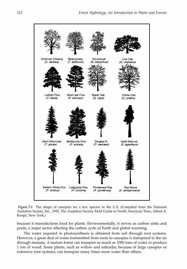
112 Forest Hydrology: An Introduction to Water and Forests
because it manufactures food for plants. Environmentally, it serves as carbon sinks andpools, a major sector affecting the carbon cycle of Earth and global warming.
The water required in photosynthesis is obtained from soil through root systems.However, a great deal of water transmitted from roots to canopies is transpired to the airthrough stomata. A mature forest can transpire as much as 1000 tons of water to produce1 ton of wood. Some plants, such as willow and saltcedar, because of large canopies orextensive root systems, can transpire many times more water than others.
Figure 7.1
The shape of canopies for a few species in the U.S. (Compiled from the NationalAudubon Society, Inc., 1992, The Audubon Society Field Guide to North American Trees, Alfred A.Knopf, New York.)
1363_C07_fm Page 112 Wednesday, December 4, 2002 7:41 AM
Chapter seven: Characteristic forests 113
Since photosynthesis and transpiration are conducted through leaves, the differencein the quantity of leaves among species is commonly expressed in terms of leaf area index(LAI), or total surface of leaf per unit land area in m
2
m
-
2
. Variations in LAI are greatamong species and within species due to differences in site quality, age, stand composition,density, and season. LAI is about 3.1 for aspens in the central Rocky Mountains (Kaufmannet al., 1982), 5.3 for a 10-year-old stand of eastern white pine (Swank and Schreuder, 1974),4.2 to 9.6 for tropical regenerating forests near Manaus, Brazilian Amazonia (Honzák et al.,1996), and 10.2 for Norway spruce in Wisconsin (Gower and Son, 1992). For a forest standwith multiple stories, LAI can go much higher than a single species. The LAI is 42 formature stands of western hemlock and silver fir in the western Oregon Cascades (Gholzet al., 1976), and 40 to 50 for a mature stand with 90% spruce and 10% fir in the centralRocky Mountains (Kaufmann et al., 1982). Many biological processes and environmentalfunctions such as transpiration, canopy interception, light penetration, heat exchange,carbon fluxes, respiration, photosynthesis, and wind movements are highly correlatedwith LAI.
2. Root systems
About 10% of the wood mass of a tree is in the form of roots under the ground (Mirov,1949), and 70% or more of the roots tend to concentrate in the A horizon (Farrish, 1991).A big spreading oak tree can have roots totaling many hundreds of kilometers. Livingroots of mesquite, a phreatophyte growing on rangeland in the Southwest, were found
Table 7.1
Biological and Environmental Functions of Canopy, Stem, and Root System
Component Biological Functions Environmental Functions
Canopy 1. Photosynthesis2. Transpiration3. Respiration4. Reproduction5. Gas exchange6. Assimilation of foods7. Food storage8. Precipitation interception9. Affecting solar radiation
dissipation10. Fog and cloud condensation11. Reducing raindrop impact to soil12. Snow accumulation and
snowmelt
1. Carbon sinks and pools2. Affecting soil moisture and infiltration3. Intercepting advective energy4. Shading5. Aesthetic value6. Shelters for birds and insects7. Barriers to wind movement
.
Stem 1. Transport water and nutrients2. Support canopies3. Help store materials4. Photosynthesis, if green5. Use for plant regeneration6. Transpiration
1. Mechanical barriers to wind and water2. Tree rings as an index for past
hydroclimatic conditions3. Mechanical support and nutrient
provider to vines, mosses, and lichens
Roots 1. Absorb water and nutrients2. Transport water and nutrients3. Anchor plant4. Store materials5. Use for plant regeneration6. Respiration7. Nitrogen fixation, if legumes
1. Reinforcement of soils2. Increase soil permeability3. Improve soil structure4. Add soil organic matter when decayed5. Slow-down overland runoff, such as
buttress roots6. Deplete soil moisture content
1363_C07_fm Page 113 Wednesday, December 4, 2002 7:41 AM
114 Forest Hydrology: An Introduction to Water and Forests
53.3 m below the original surface of an open-pit mine in Arizona (Phillips, 1963) andcommonly spread more than 15 m wide from a single tree. The root mass beneath the rootcrown of a shrub live oak, the zone occupied by the taproot, reached 99 kg/m
3
of soil inArizona (Davis and Pase, 1977). Those deep and widespread roots are able to use ephem-eral surface soil moisture, moisture deep in the soil, and groundwater.
In the Harvard Black Rock Forest, New York, the average surface coverage of the rootsystems was about 4.5 times greater than the ground surface covered by the canopies for25 mature hardwood trees. A sprout clump of chestnut oak, 17 years old and 10 m inheight, had a root system that covered 57 m
2
surface area and was about 41 times greaterthan the ground area covered by its canopies (Stout, 1956). Differences in the depth, surfacecoverage, and density of root systems are reflections of species and a variety of environ-mental factors such as soil texture, depth, moisture content, nutrients, groundwater table,and plant competition. Sprouting shrub species tend to have deeper roots than nonsprout-ing species (Keeley and Keeley, 1998).
Root systems are an important factor affecting soil properties, surface hydrology, andslope stability. Large roots can anchor the plant and soil mantle to the substrate, whilefine roots, fungal mycelia, and decomposed organic matter can contribute to the formationof stable aggregates for subsurface soils. The improvement of soil granulation may be dueto: (1) pressure exerted by growing roots, (2) the dehydration of the soil around rootsystems, and (3) secretion of substances produced by roots and accompanying bacteriathat bind and cement soil aggregates.
Roots grow and die every year. The dead roots, root secretions, and fallen litter,through microbial activities, become important parts of organic matter in the soil. Theyprovide a physical environment suitable for a vast array of plants and animals in varioussizes. The large population of macro- and microorganisms in and around the soil promotethe decomposition of organic matter, the mixing of organic matter and inorganic surfacesoil, the creation of soil organic horizon, and the improvement of the soil’s physical andchemical properties. As a result, soil porosity, infiltration capacity, soil water-holdingcapacity, and plant transpiration are increased, and surface runoff is reduced.
Plants enhance soil stability against downslope movement due to the reduction of soilwater content through transpiration and the mechanical reinforcement of the root system(Waldron and Dakessian, 1982). Roots increase the cohesive and frictional components ofthe soil’s shear strength, which is a force counter to the force causing the soil to movedownslope. The increase in soil shear strength is proportional to the fresh weight of rootsper unit volume of soil. Trees usually exert a greater strength than grasses, and the removalof trees causes a decrease in root tensile strength due to the decay of root systems. Manylandslides in New Zealand and the northwestern U.S. were attributed to forest removals(Sidle et al, 1985). Plant roots provide most of the shear strength for soil stability alongstream banks (Kleinfelder et al., 1992).
3. Stems
Forest trees usually have a single stem; its environmental functions are far fewer thanthose of the canopy and the root. Stems can impose mechanical disruptions to wind andwater movements; however, the effectiveness is largely dependent upon the diameter anddensity of stems in the area. Some of the environmental functions of canopies are affectedby stem height. Since the stem accounts for about 80% or more of the biomass of a singletree, carbon storage can be an important environmental function of stems.
The total area of closed and open tropical forests is about 1.929
¥
10
6
ha, which containsa total stemwood biomass of about 119.89
¥
10
9
tons. Assuming 1 ton of organic matter isequivalent to 0.5 tons of organic carbon (Brown and Lugo, 1984; Brown et al., 1989), thestemwood in the tropical forests contains 59.96
¥
10
9
tons or 31.08 tons/ha of carbon. The
1363_C07_fm Page 114 Wednesday, December 4, 2002 7:41 AM
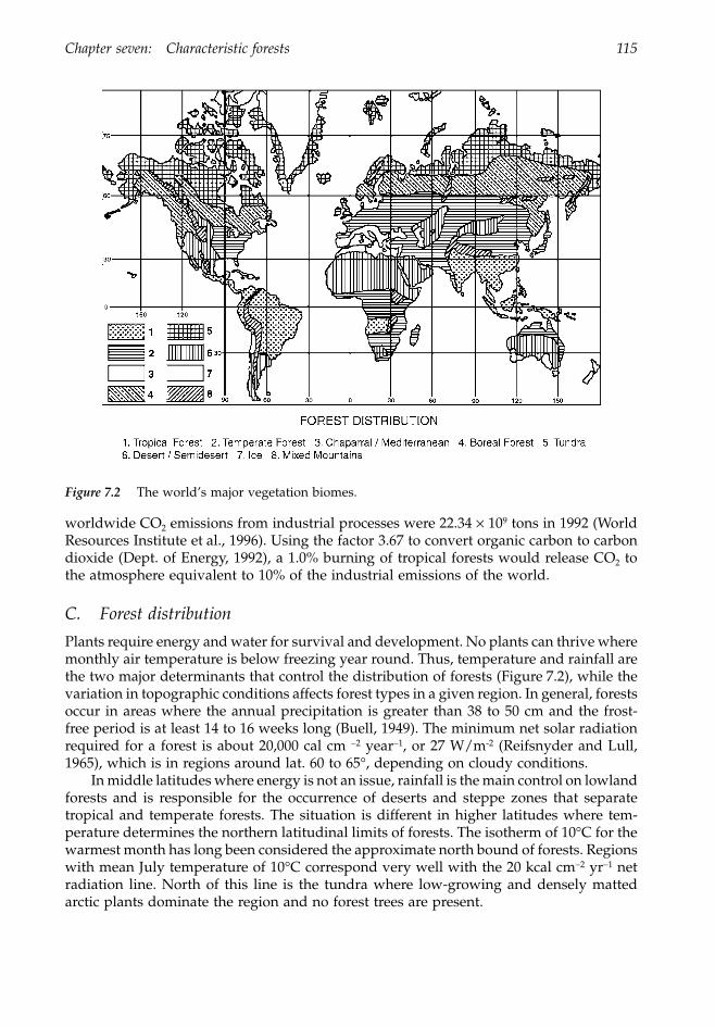
Chapter seven: Characteristic forests 115
worldwide CO
2
emissions from industrial processes were 22.34
¥
10
9
tons in 1992 (WorldResources Institute et al., 1996). Using the factor 3.67 to convert organic carbon to carbondioxide (Dept. of Energy, 1992), a 1.0% burning of tropical forests would release CO
2
tothe atmosphere equivalent to 10% of the industrial emissions of the world.
C. Forest distribution
Plants require energy and water for survival and development. No plants can thrive wheremonthly air temperature is below freezing year round. Thus, temperature and rainfall arethe two major determinants that control the distribution of forests (Figure 7.2), while thevariation in topographic conditions affects forest types in a given region. In general, forestsoccur in areas where the annual precipitation is greater than 38 to 50 cm and the frost-free period is at least 14 to 16 weeks long (Buell, 1949). The minimum net solar radiationrequired for a forest is about 20,000 cal cm
-
2
year
-
1
, or 27 W/m
-2
(Reifsnyder and Lull,1965), which is in regions around lat. 60 to 65
∞
, depending on cloudy conditions.In middle latitudes where energy is not an issue, rainfall is the main control on lowland
forests and is responsible for the occurrence of deserts and steppe zones that separatetropical and temperate forests. The situation is different in higher latitudes where tem-perature determines the northern latitudinal limits of forests. The isotherm of 10
∞
C for thewarmest month has long been considered the approximate north bound of forests. Regionswith mean July temperature of 10
∞
C correspond very well with the 20 kcal cm
-
2
yr
-
1
netradiation line. North of this line is the tundra where low-growing and densely mattedarctic plants dominate the region and no forest trees are present.
Figure 7.2
The world’s major vegetation biomes.
1363_C07_fm Page 115 Wednesday, December 4, 2002 7:41 AM
116 Forest Hydrology: An Introduction to Water and Forests
1. Horizontal distribution
On the latitudinal scale there are three zones of great precipitation. The greatest zoneoccurs in the equatorial areas and two secondary zones are in the high latitudes aroundlat. 50
∞
N and lat. 50
∞
S. The precipitation patterns cause the majority of Earth’s forests tobe distributed in two regions, one in the tropical areas and the other in the North Hemi-sphere roughly between 35
∞
and 65
∞
latitudes. According to the temperature regimes,forests are broadly grouped into three major types: tropical, temperate, and boreal.
a. Tropical forests.
The tropical regions are bounded roughly between the Tropicof Cancer (lat. 23.5
∞
N) and the Tropic of Capricorn (lat. 23.5
∞
S), where the mean temper-ature of the coldest month is at least 18
∞
C, and precipitation tends to decrease outwardfrom the equatorial region. Accordingly, there is a vegetation gradient from tropical rainforests (evergreen) in the equatorial zone to tropical seasonal forests, tropical scrub forests,and tropical savannah forests.
Tropical rain forests are found in the Amazon Basin, Southeast Asia, and central Africa.Here the climate is hot and damp throughout the year, plant growth is profuse, thediversity of tree species is high, plant litter deposition is very rapid, and soils are old,weathered, and well leached. Outward from the equatorial areas is the tropical seasonalforest where dry seasons are clear and pronounced. Tropical seasonal forests are welldistributed in the northern part of South America, from northeast India to Burma andnorthern Australia, and from Angola to Tanzania in south-central Africa. The forest issimpler and lower than either semievergreen or deciduous rain forest. Tropical deciduousforests, also known as monsoon forests, are in areas where there is a distinguished dryseason in the year, all the arboreal species are deciduous, and the ground is bare for longor short periods of time.
Tropical scrub forests occur in regions of light rainfall, bordering wet forests in thesouth and deserts in the north. They run roughly along lat. 10 to 14
∞
N in north-centralAfrica, South Africa, and southern Australia. Small leaved evergreen vegetation withwarm and wet winters, and long, dry summers dominate the forest. Where the dry seasonlasts on the order of 6 months, a mixture of trees and grasslands called savanna forestsoccur. The savanna forests, dominated by grasses and sedges with open stands of well-spaced trees, are widespread in Africa and in southern Brazil.
b. Temperate forests.
Forests in the Temperate Zone can be grouped into fivetypes: deciduous, coniferous, broad-leaved evergreen, mixed evergreen, and Mediterra-nean. Here, winter is distinct, growing seasons are long, and precipitation exceeds evapo-transpiration. Climate changes from season to season and within each season as well.Temperate deciduous broad-leaved forests are distributed in regions with 4 to 6 frost-freemonths and precipitation either relatively even throughout the year or higher in thesummer. They occur in western and central Europe, eastern North America, and north-eastern Asia. Coniferous forests are found mainly in North America, stretching fromMinnesota to New England, much of the coastal plains from New Jersey to east Texas,and the Pacific coast from Alaska to British Columbia, Washington, Oregon and northernCalifornia. The winter is mild and precipitation in winter is higher than in the summerin these areas.
In areas where winter is mild and wet, summer is warm and dry, and annual rainfallis less than 1000 mm in general, forests tend to be dominated by mixed evergreen conif-erous and broad-leaved species, the so-called “Mediterranean forests.” They can be foundin Mediterranean basins, western and southwestern North America, temperate Asia, andAustralia. However, west of the Mediterranean climate and along the coastal areas fromnorthern California to southeast Alaska, their precipitation remains concentrated in the
1363_C07_fm Page 116 Wednesday, December 4, 2002 7:41 AM
Chapter seven: Characteristic forests 117
winter but reaches from 1500 to over 2000 mm/year. Here, redwoods, Douglas fir, hemlock,and Sitka spruce are mixed with evergreen hardwood species. These forests are some ofthe most long-lived and productive in the world, longer in life and production than manytropical rain forests (Perry, 1994).
Evergreen broad-leaved forests occur mainly in southern China, the lower slopes ofthe Himalayas, southern Japan, southeastern U.S., much of southeast and southwestAustralia, New Zealand, and southern coast of Chile. All these areas have mild temper-atures, frost-free winters, and relatively high precipitation (>1500 mm/year).
c. Boreal Forests.
North of the temperate forest where winter temperature is toocold and growing seasons are too short to support hardwood species, cold-tolerant conifersknown as the boreal forests become dominant. Typically, the boreal forests develop inareas with about 6 months of below freezing temperatures, 50 to 125 days of the growingseason, 1 to 3 months of mean summer temperature above 10
∞
C, and 35 to 50 cm of annualprecipitation. They are distributed in two bands, one in North America from Alaska toNewfoundland and the other in Eurasia from the Atlantic coast of Scandinavia to thePacific coast of Siberia, roughly between lat. 50
∞
N and lat. 60
∞
N.The boreal forests are a lot simpler and more uniform than forests in other regions.
Species of spruce, fir, larch, and pine are numerically dominant throughout most of theforests. Contrary to the 4 years for temperate deciduous forests and 0.7 years for tropicforests, the mean residence time of organic matter on the forest floor for boreal forests is350 years (Mather, 1990). Thus, most of nutrients in the boreal forests, not like those intropical forests, are contained in the litter, not in the vegetation. The boreal coniferousforests are by far the most extensive remaining forests outside of the tropical forests.
2. Vertical distribution
In the free air — air not in contact with the ground — there is a fairly uniform decreaseof temperature with increasing elevation. The rate of temperature decrease is about, onthe average, 0.65
∞
C/100 m. This is called the normal lapse rate or vertical temperaturegradient. On the horizontal scale, the temperature gradient between lat. 20
∞
N and lat. 80
∞
N varies from
-
0.5 to
-
1.0
∞
C/1
∞
latitude. This means that a mountain at lat. 20
∞
N whereits mean base surface annual temperature is 25.3
∞
C would have a mean annual temperatureof 5.8
∞
C at 3000 m, a thermal climate equivalent to temperate zone at lat. 50
∞
N (Figure 7.3).Also, due to orographic effects, precipitation is greater on windward slopes and at
higher elevations of the mountain. However, the greater precipitation at higher elevationsoccurs only up to a certain level. Above this level, the air humidity is too low, precipitationdeclines, and the environmental harshness increases with height. Therefore, precipitationand temperature variation cause changes in forest types along an elevation gradient inmountainous areas.
At a sufficient height, harsh environmental conditions such as short growing seasons,frigid air and soil temperatures, low available water, high wind speed, and deficient carbondioxide can cause the abrupt termination of a closed forest stand. Beyond this forest limit,or the so-called timberline, tundra and alpine vegetation predominate. Forest types belowthe timberline start with conifers, mixed conifers and hardwoods, hardwoods, shrubs,grasslands or deserts, and tropical rain forests, depending on latitude, height of themountain, and distance to the ocean. This vertical distribution of vegetation can beuniquely illustrated by the slopes of the central Sierra Nevada in California (Figure 7.4).Rising to more than 3965 m, over a dozen distinct plant zones have been identified betweenthe base and the mountain peak.
The height of timberline is 900 m at Haines, Alaska (lat. 60
∞
N); 1850 to 1900 m at GaribaldiPark, British Columbia (lat. 50
∞
N); 3300 m at the Sierra Nevada mountains, California (lat.
1363_C07_fm Page 117 Wednesday, December 4, 2002 7:41 AM
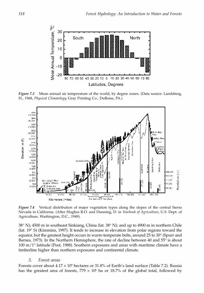
118 Forest Hydrology: An Introduction to Water and Forests
38
∞
N); 4500 m in southeast Sinkiang, China (lat. 38
∞
N); and up to 4900 m in northern Chile(lat. 19
∞
S) (Kimmins, 1997). It tends to increase in elevation from polar regions toward theequator, but the greatest height occurs in warm-temperate belts, around 25 to 30
∞
(Spurr andBarnes, 1973). In the Northern Hemisphere, the rate of decline between 40 and 55
∞
is about100 m/1
∞
latitude (Peet, 1988). Southern exposures and areas with maritime climate have atimberline higher than northern exposures and continental climate.
3. Forest areas
Forests cover about 4.17
¥
10
9
hectares or 31.8% of Earth’s land surface (Table 7.2). Russiahas the greatest area of forests, 779
¥
10
6
ha or 18.7% of the global total, followed by
Figure 7.3
Mean annual air temperature of the world, by degree zones. (Data source: Landsberg,H., 1968,
Physical Climatology
, Gray Printing Co., DuBoise, PA.)
Figure 7.4
Vertical distribution of major vegetation types along the slopes of the central SierraNevada in California. (After Hughes R.O. and Dunning, D. in
Yearbook of Agriculture
, U.S. Dept. ofAgriculture, Washington, D.C., 1949).
1363_C07_fm Page 118 Wednesday, December 4, 2002 7:41 AM
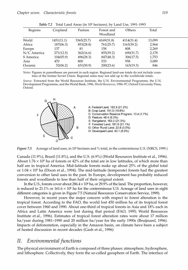
Chapter seven: Characteristic forests 119
Canada (11.9%), Brazil (11.8%), and the U.S. (6.9%) (World Resources Institute et al., 1996).About 1.76
¥
10
9
ha of forests or 42% of the total are in low latitudes, of which more thanhalf are in tropical America. Mid-latitude forests make up about 25% of the global totalor 1.04
¥
10
9
ha (Dixon et al., 1994). The mid-latitude (temperate) forests had the greatestconversion to other land uses in the past. In Europe, development has probably reducedforests and woodlands to less than half of their original extent.
In the U.S., forests cover about 286.4
¥
10
6
ha, or 29.9% of the land. The proportion, however,is reduced to 21.1% or 161.6
¥
10
6
ha for the conterminous U.S. Acreage of land uses in eightdifferent categories is given in Figure 7.5 (Natural Resources Conservation Service, 1999).
However, in recent years the major concern with respect to forest alteration is thetropical forest. According to the FAO, the world lost 450 million ha of its tropical forestcover between 1960 and 1990. About one-third of tropical forests in Asia and 18% each inAfrica and Latin America were lost during that period (FAO, 1995; World ResourcesInstitute et al., 1996). Estimates of tropical forest alteration rates were about 17 millionha/year during 1981–1990 and 20 million ha/year for the early 1990s (Bruijnzeel, 1996).Impacts of deforestation, especially in the Amazon basin, on climate have been a subjectof heated discussion in recent decades (Gash et al., 1996)
II. Environmental functions
The physical environment of Earth is composed of three phases: atmosphere, hydrosphere,and lithosphere. Collectively, they form the so-called geosphere of Earth. The interface of
Table 7.2
Total Land Areas (in 10
6
hectares), by Land Use, 1991–1993
Regions Cropland Pasture Forest and Woodland
Others Total
World 1451(11.1) 3365(25.7) 4169(31.8) 4114(31.4) 13,099Africa 187(06.3) 853(28.8) 761(25.7) 1163(39.2) 2,964Europe 137 81 158 808 2,269N/C America 271(12.5) 362(16.6) 855(39.2) 690(31.7) 2,178S America 104(05.9) 496(28.3) 847(48.3) 306(17.5) 1,753Asia 470 800 533 958 3,089Oceania 52(06.2) 431(50.9) 200(23.6) 163(19.3) 846
Notes:
Figures in parentheses are percent in each region. Regional land-use totals do not include coun-tries of the former Soviet Union. Regional sums may not add up to the worldwide totals.
Source:
Extracted from the World Resources Institute, the U.N. Environmental Programme, the U.N.Development Programme, and the World Bank, 1996,
World Resources
, 1996–97, Oxford University Press,Oxford.
Figure 7.5
Acreage of land uses, in 10
6
hectares and % total, in the conterminous U.S. (NRCS, 1999.)
1363_C07_fm Page 119 Wednesday, December 4, 2002 7:41 AM
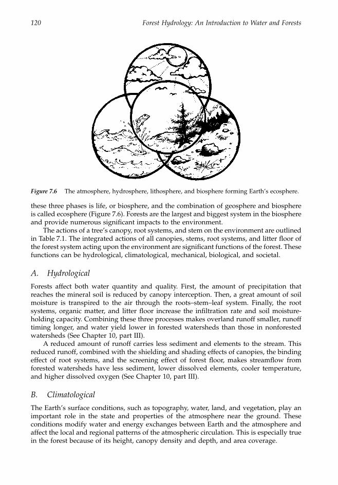
120 Forest Hydrology: An Introduction to Water and Forests
these three phases is life, or biosphere, and the combination of geosphere and biosphereis called ecosphere (Figure 7.6). Forests are the largest and biggest system in the biosphereand provide numerous significant impacts to the environment.
The actions of a tree’s canopy, root systems, and stem on the environment are outlinedin Table 7.1. The integrated actions of all canopies, stems, root systems, and litter floor ofthe forest system acting upon the environment are significant functions of the forest. Thesefunctions can be hydrological, climatological, mechanical, biological, and societal.
A. Hydrological
Forests affect both water quantity and quality. First, the amount of precipitation thatreaches the mineral soil is reduced by canopy interception. Then, a great amount of soilmoisture is transpired to the air through the roots–stem–leaf system. Finally, the rootsystems, organic matter, and litter floor increase the infiltration rate and soil moisture-holding capacity. Combining these three processes makes overland runoff smaller, runofftiming longer, and water yield lower in forested watersheds than those in nonforestedwatersheds (See Chapter 10, part III).
A reduced amount of runoff carries less sediment and elements to the stream. Thisreduced runoff, combined with the shielding and shading effects of canopies, the bindingeffect of root systems, and the screening effect of forest floor, makes streamflow fromforested watersheds have less sediment, lower dissolved elements, cooler temperature,and higher dissolved oxygen (See Chapter 10, part III).
B. Climatological
The Earth’s surface conditions, such as topography, water, land, and vegetation, play animportant role in the state and properties of the atmosphere near the ground. Theseconditions modify water and energy exchanges between Earth and the atmosphere andaffect the local and regional patterns of the atmospheric circulation. This is especially truein the forest because of its height, canopy density and depth, and area coverage.
Figure 7.6
The atmosphere, hydrosphere, lithosphere, and biosphere forming Earth’s ecosphere.
1363_C07_fm Page 120 Wednesday, December 4, 2002 7:41 AM
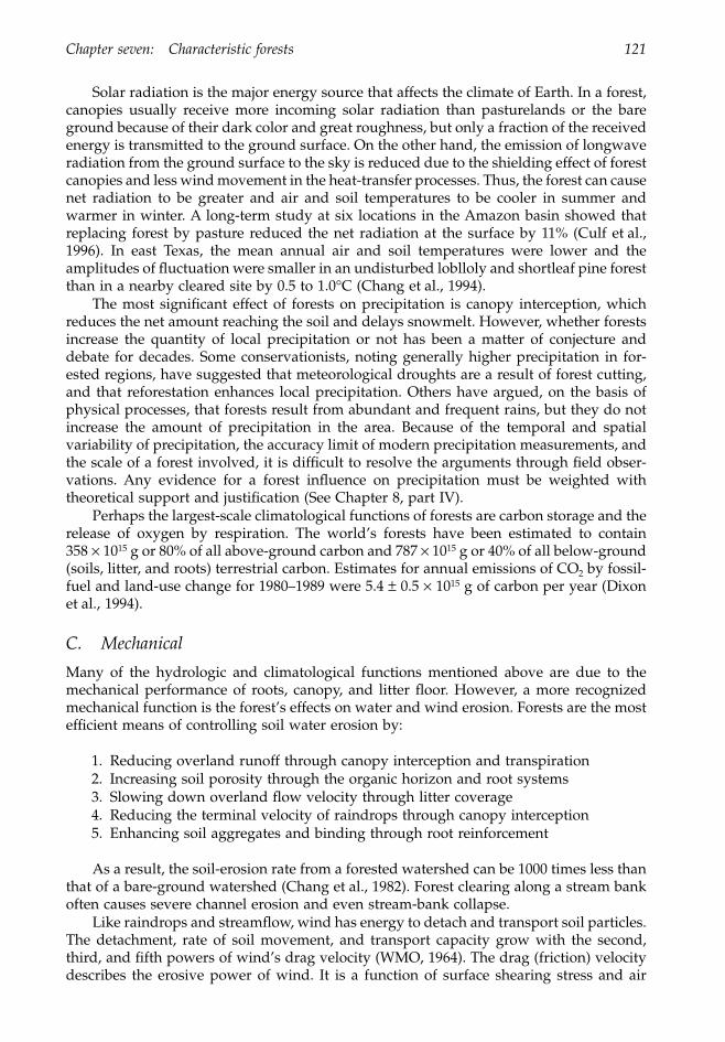
Chapter seven: Characteristic forests 121
Solar radiation is the major energy source that affects the climate of Earth. In a forest,canopies usually receive more incoming solar radiation than pasturelands or the bareground because of their dark color and great roughness, but only a fraction of the receivedenergy is transmitted to the ground surface. On the other hand, the emission of longwaveradiation from the ground surface to the sky is reduced due to the shielding effect of forestcanopies and less wind movement in the heat-transfer processes. Thus, the forest can causenet radiation to be greater and air and soil temperatures to be cooler in summer andwarmer in winter. A long-term study at six locations in the Amazon basin showed thatreplacing forest by pasture reduced the net radiation at the surface by 11% (Culf et al.,1996). In east Texas, the mean annual air and soil temperatures were lower and theamplitudes of fluctuation were smaller in an undisturbed loblloly and shortleaf pine forestthan in a nearby cleared site by 0.5 to 1.0
∞
C (Chang et al., 1994).The most significant effect of forests on precipitation is canopy interception, which
reduces the net amount reaching the soil and delays snowmelt. However, whether forestsincrease the quantity of local precipitation or not has been a matter of conjecture anddebate for decades. Some conservationists, noting generally higher precipitation in for-ested regions, have suggested that meteorological droughts are a result of forest cutting,and that reforestation enhances local precipitation. Others have argued, on the basis ofphysical processes, that forests result from abundant and frequent rains, but they do notincrease the amount of precipitation in the area. Because of the temporal and spatialvariability of precipitation, the accuracy limit of modern precipitation measurements, andthe scale of a forest involved, it is difficult to resolve the arguments through field obser-vations. Any evidence for a forest influence on precipitation must be weighted withtheoretical support and justification (See Chapter 8, part IV).
Perhaps the largest-scale climatological functions of forests are carbon storage and therelease of oxygen by respiration. The world’s forests have been estimated to contain358
¥
10
15
g or 80% of all above-ground carbon and 787
¥
10
15
g or 40% of all below-ground(soils, litter, and roots) terrestrial carbon. Estimates for annual emissions of CO
2
by fossil-fuel and land-use change for 1980–1989 were 5.4
±
0.5
¥
10
15
g of carbon per year (Dixonet al., 1994).
C. Mechanical
Many of the hydrologic and climatological functions mentioned above are due to themechanical performance of roots, canopy, and litter floor. However, a more recognizedmechanical function is the forest’s effects on water and wind erosion. Forests are the mostefficient means of controlling soil water erosion by:
1. Reducing overland runoff through canopy interception and transpiration2. Increasing soil porosity through the organic horizon and root systems3. Slowing down overland flow velocity through litter coverage4. Reducing the terminal velocity of raindrops through canopy interception5. Enhancing soil aggregates and binding through root reinforcement
As a result, the soil-erosion rate from a forested watershed can be 1000 times less thanthat of a bare-ground watershed (Chang et al., 1982). Forest clearing along a stream bankoften causes severe channel erosion and even stream-bank collapse.
Like raindrops and streamflow, wind has energy to detach and transport soil particles.The detachment, rate of soil movement, and transport capacity grow with the second,third, and fifth powers of wind’s drag velocity (WMO, 1964). The drag (friction) velocitydescribes the erosive power of wind. It is a function of surface shearing stress and air
1363_C07_fm Page 121 Wednesday, December 4, 2002 7:41 AM
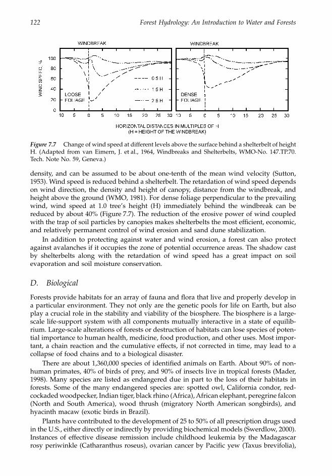
122 Forest Hydrology: An Introduction to Water and Forests
density, and can be assumed to be about one-tenth of the mean wind velocity (Sutton,1953). Wind speed is reduced behind a shelterbelt. The retardation of wind speed dependson wind direction, the density and height of canopy, distance from the windbreak, andheight above the ground (WMO, 1981). For dense foliage perpendicular to the prevailingwind, wind speed at 1.0 tree’s height (H) immediately behind the windbreak can bereduced by about 40% (Figure 7.7). The reduction of the erosive power of wind coupledwith the trap of soil particles by canopies makes shelterbelts the most efficient, economic,and relatively permanent control of wind erosion and sand dune stabilization.
In addition to protecting against water and wind erosion, a forest can also protectagainst avalanches if it occupies the zone of potential occurrence areas. The shadow castby shelterbelts along with the retardation of wind speed has a great impact on soilevaporation and soil moisture conservation.
D. Biological
Forests provide habitats for an array of fauna and flora that live and properly develop ina particular environment. They not only are the genetic pools for life on Earth, but alsoplay a crucial role in the stability and viability of the biosphere. The biosphere is a large-scale life-support system with all components mutually interactive in a state of equilib-rium. Large-scale alterations of forests or destruction of habitats can lose species of poten-tial importance to human health, medicine, food production, and other uses. Most impor-tant, a chain reaction and the cumulative effects, if not corrected in time, may lead to acollapse of food chains and to a biological disaster.
There are about 1,360,000 species of identified animals on Earth. About 90% of non-human primates, 40% of birds of prey, and 90% of insects live in tropical forests (Mader,1998). Many species are listed as endangered due in part to the loss of their habitats inforests. Some of the many endangered species are: spotted owl, California condor, red-cockaded woodpecker, Indian tiger, black rhino (Africa), African elephant, peregrine falcon(North and South America), wood thrush (migratory North American songbirds), andhyacinth macaw (exotic birds in Brazil).
Plants have contributed to the development of 25 to 50% of all prescription drugs usedin the U.S., either directly or indirectly by providing biochemical models (Swerdlow, 2000).Instances of effective disease remission include childhood leukemia by the Madagascarrosy periwinkle (Catharanthus roseus), ovarian cancer by Pacific yew (Taxus brevifolia),
Figure 7.7 Change of wind speed at different levels above the surface behind a shelterbelt of heightH. (Adapted from van Eimern, J. et al., 1964, Windbreaks and Shelterbelts, WMO-No. 147.TP.70.Tech. Note No. 59, Geneva.)
1363_C07_fm Page 122 Wednesday, December 4, 2002 7:41 AM

Chapter seven: Characteristic forests 123
dementia by ginkgo (Ginkgo biloba), malaria by qing hao (Artemisia annua), tumor andcancer activity by happytrees (Camptotheca acuminata), and many others. In China, herbalmedicine has been practiced for more than 5000 years. Li Shih Tseng wrote the bookOutlines of Medicinal Plants in 1595 (the Ming Dynasty). It listed 1097 drugs extractedfrom 512 plant species and 11,096 prescriptions for botanical remedies or pharmaceuticaltreatments. Some utilized plants’ roots and bark, while others used leaves, flowers, shoots,nuts, fruits, fruit skins, stems, and sap. The U.S. National Cancer Institute has identified3000 plants as potential sources for cancer-fighting chemicals.
E. Societal
Cool and shaded forests, with their vast area, wilderness setting, and fresh air are idealplaces for people to relax from tension, pressure, and hectic activities. Green canopies withblue sky and white clouds are a natural beauty to our eyes, and the environmentaltranquility relaxes our ears and minds. Thus, many recreation and leisure-time activities— picnicking, sightseeing, bird watching, hiking, camping, and canoeing — take place inforest areas. Psychologists have even used “forest bath,” a mental bath in the forestenvironment, as a treatment for persons with depression. Retreating from hectic cities towilderness has become a part of lifestyle in modern societies.
The presence of forests can benefit the health of people living in their vicinity. Thismay be attributable to the continuous replenishment of oxygen and the reduction of dustand air pollutants in forested areas. City and traffic noise can be attenuated and unsightlyenvironments can be blocked by a greenbelt of trees.
Wilderness areas serve as field laboratories for various research and educationalpurposes. They provide opportunities for the public to study and appreciate forest eco-systems, ecological processes, habitats, landscapes, and natural-resources conservation.
III. Functional forestsAlthough forests perform many environmental functions, some functions may be moresignificant than others for a particular forest because of its location and environment.Thus, a forest may be intentionally managed to maximize one or two specific functions,with little attention paid to others. It can be described as a functional forest.
Functional forests can be grouped into four categories: production forests, protectionforests, preservation forests, and public forests. The functions that a forest is managed toperform are mostly a matter of site and environmental conditions. Frequently, however,the ownership, economic constraints, and prospective value of the forest play an importantrole in determining management objectives. Also, many environmental regulations andgovernmental policies provide guidelines for managing forest resources. For example, theMultiple-Use and Sustained Yield Act of 1960 requires that the national forests be estab-lished and administered for outdoor recreation, range, timber, watershed, wildlife, andfish purposes. The National Forest Management Act of 1976 further strengthened multiple-use practices in the national forests. Multiple uses are less emphasized in private andindustrial forests.
A. Production forests
The main purpose of production forests is to obtain financial profit from the forest byproducing timber, pulpwood, fuels, wildlife, forest and agricultural byproducts, livestock,and recreation services. In the U.S., production forests are owned and operated mainlyby private individuals (57%) and industry (15%), while only 28% are national and public
1363_C07_fm Page 123 Wednesday, December 4, 2002 7:41 AM
124 Forest Hydrology: An Introduction to Water and Forests
forests (MacCleery, 1993). Traditionally, the primary concern of industrial and privateowners is timber production. Only in recent decades have other products and servicesbecome a serious consideration in maximizing forest incomes. Today, hunting for a fee isavailable in many private forest clubs throughout the nation, and many ranchers andcabins nestled in forested areas are operated for families to spend a weekend in the forestfor relaxation, enjoyment, and outdoor activities.
In rural areas of the tropical regions, a sizeable population lives in and around forests.They grow crops in the forest for food and harvest branch and litter for fuel. India hasbegun a social program in which people plant and grow trees in their back yards andcommunity woodlots for fuel and other purposes. Many feasibility studies have shownthat power stations could be operated and the liquid fuel ethanol could be produced basedon trees growing in “energy plantations” (Fung, 1982). Forest grazing is also a commonpractice that often damages trees, destroys litter floor, and compacts soils. These exploit-ative agroforestry practices interrupt nutrient cycling in the forest, increase soil and watererosion, deplete land productivity, and eventually lead to the abandonment of forests forproduction. In northeastern India alone, about 2,600,000 people depend on shifting culti-vation, affecting about 2,700,000 ha of forestland (Shafi, 1992).
In the pursuit of maximum economic gain from a forest, exploitative uses of itsresources should be avoided. Best-management practices should be incorporated in allforestry activities so that land productivity can be maintained and water quality is notimpaired. The U.S. Forest Service adopted ecosystem management as a policy in June1992. The ecosystem-management approach is to use ecological principles and the bestavailable science and technology in managing natural resources. It recognizes soil, water,vegetation, wildlife, society, and the economy as integrated factors in the formulation ofmanagement objectives. Experience from the national forests can serve as guidelines tomanaging private forests.
B. Protection forests
On rough terrain, steep slopes, stream banks, water-resource areas, wind-prone regions,or potential landslide sites, forests are often established to reduce soil erosion, increasesand stability, improve water quality, retain reservoir capacity, mitigate flood damage, andattenuate air pollution. Forests are also managed to protect habitats for birds, fish, andother animals. Protection forests emphasize environmental functions; economic income isinsignificant or even totally ignored. In India, protection forests make up about 23.4% or15 ¥ 106 ha of the nation’s forests (Lal, 1992).
Since protection forests are there to protect a specific site and environmental condition,species used are more restrictive, and management activities need to assure the sustain-ability of the forest. For example, salt spray, high wind speed with abrasive sands, lowfertility, high temperature, and extremely wet and dry soil conditions are the generalcharacteristics of coastal sand dunes. Because of their adaptability, species such as sandlive oak (Q. virginiana) and southern waxmyrtle (Myrica cerifera) in the south Atlantic coastand casuarina (Casuarina equisetifolia) in Taiwan are often planted to protect against winderosion and sand-dune movement in coastal areas. Protection forests are usually in areassensitive to environmental problems; clearcutting, grazing, cropping, and litter harvestingshould not be practiced. A clearcut in these sensitive areas would make artificial regen-eration very difficult or too long to establish. It can consequently make the destruction offorests in the protected area devastating. Thus, legal enforcement may be required toprevent protection forests from damage by cultivation, harvesting, grazing, and otherimpairing activities.
1363_C07_fm Page 124 Wednesday, December 4, 2002 7:41 AM
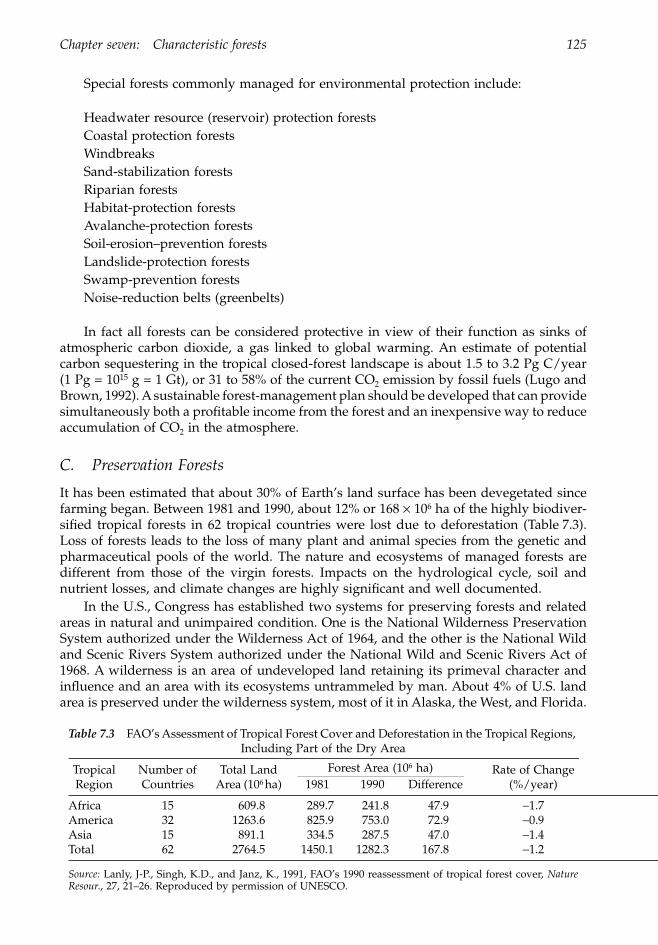
Chapter seven: Characteristic forests 125
Special forests commonly managed for environmental protection include:
Headwater resource (reservoir) protection forestsCoastal protection forestsWindbreaksSand-stabilization forestsRiparian forestsHabitat-protection forestsAvalanche-protection forestsSoil-erosion–prevention forestsLandslide-protection forestsSwamp-prevention forestsNoise-reduction belts (greenbelts)
In fact all forests can be considered protective in view of their function as sinks ofatmospheric carbon dioxide, a gas linked to global warming. An estimate of potentialcarbon sequestering in the tropical closed-forest landscape is about 1.5 to 3.2 Pg C/year(1 Pg = 1015 g = 1 Gt), or 31 to 58% of the current CO2 emission by fossil fuels (Lugo andBrown, 1992). A sustainable forest-management plan should be developed that can providesimultaneously both a profitable income from the forest and an inexpensive way to reduceaccumulation of CO2 in the atmosphere.
C. Preservation Forests
It has been estimated that about 30% of Earth’s land surface has been devegetated sincefarming began. Between 1981 and 1990, about 12% or 168 ¥ 106 ha of the highly biodiver-sified tropical forests in 62 tropical countries were lost due to deforestation (Table 7.3).Loss of forests leads to the loss of many plant and animal species from the genetic andpharmaceutical pools of the world. The nature and ecosystems of managed forests aredifferent from those of the virgin forests. Impacts on the hydrological cycle, soil andnutrient losses, and climate changes are highly significant and well documented.
In the U.S., Congress has established two systems for preserving forests and relatedareas in natural and unimpaired condition. One is the National Wilderness PreservationSystem authorized under the Wilderness Act of 1964, and the other is the National Wildand Scenic Rivers System authorized under the National Wild and Scenic Rivers Act of1968. A wilderness is an area of undeveloped land retaining its primeval character andinfluence and an area with its ecosystems untrammeled by man. About 4% of U.S. landarea is preserved under the wilderness system, most of it in Alaska, the West, and Florida.
Table 7.3 FAO’s Assessment of Tropical Forest Cover and Deforestation in the Tropical Regions, Including Part of the Dry Area
Tropical Region
Number of Countries
Total Land Area (106 ha)
Forest Area (106 ha) Rate of Change (%/year)1981 1990 Difference
Africa 15 609.8 289.7 241.8 47.9 -1.7America 32 1263.6 825.9 753.0 72.9 -0.9Asia 15 891.1 334.5 287.5 47.0 -1.4Total 62 2764.5 1450.1 1282.3 167.8 -1.2
Source: Lanly, J-P., Singh, K.D., and Janz, K., 1991, FAO’s 1990 reassessment of tropical forest cover, NatureResour., 27, 21–26. Reproduced by permission of UNESCO.
1363_C07_fm Page 125 Wednesday, December 4, 2002 7:41 AM

126 Forest Hydrology: An Introduction to Water and Forests
The preserved areas can be used only for recreational activities such as hunting, fishing,camping, and rafting, and for scientific studies and educational programs. They are freefrom any development and management, even for disease and insect salvages. Harvesting,logging, road construction, mining, damming, mechanized transport, and other commer-cial activities are prohibited.
The Scenic Rivers System allows river segments with outstanding recreational, scenic,geological, wildlife, ecological, historical, or cultural values to be protected from devel-opment and alteration. They are used for enjoyment and recreational activities such ascamping, swimming, fishing, and hunting. The river segments under the systems maynot be dammed, diverted, straightened, widened, dredged, or filled. Currently, riversegments totalling 17,490 km in length, or 0.31% of the 5.6 ¥ 106 km of rivers in the U.S.,are protected under the system.
D. Public forests
Forests that are developed and managed for the public to enjoy are referred to as publicforests. They may include parks, botanic gardens, zoos, and wildlife refuges. The majorityof public forests are national, state, and city parks. In 1872 the federal government setaside over 8 ¥ 106 ha of forest as Yellowstone National Park in northwestern Wyoming,the first national park of the world. Today there are 54 major national parks in the U.S.and over 1100 national parks of at least 1000 ha each in more than 120 countries aroundthe world (Miller, 1999).
The national parks are dedicated to preserving vegetation, wildlife, natural wonders,cultural heritages, and historical sites for people’s pleasure and health. They also provideeducational programs through forest trails, on-site written explanations, and viable envi-ronmental interpretation as well as a natural setting for ecological research and natural-resources studies. All preservation, development, and management are allowed throughintegral plans administered through the National Park Service.
IV. Threats to forestsThe most serious threats to the forests, such as deforestation, grazing, forest fires, andair pollution, come from human activities. Naturally induced insects, disease, tornadoes,volcanic eruptions, and winter storms can cause substantial damage to forests; however,their effects are, in general, not a widespread threat to the forest. Weakened trees createdby overcrowding, age, or other agents are less resistant to insect and disease attacks. Theirpopulations build up easily in these weakened trees and then spread to the entire forest.In many cases, poor forest management can cause insects and diseases. For example, asevere winter storm may cause a massive wind-throw of timber in forested areas. Unlessactive salvage actions are taken, potential for insect infestations and wildfire outbreaksis great.
A. Deforestation and grazing
In the lower latitudes, because of population and economic pressures, deforestation andgrazing caused a net loss of tropical forests of 167.8 ¥ 106 ha in the 1980s (Table 7.3). Theseforests were lost in most cases to shifting cultivation. In the middle latitudes, however,reforestation and conservation programs increased temperate forests and other woodlandsby 0.23 ¥ 106 ha in the same period (World Resources Institute et al., 1996). Thus, defor-estation and forest grazing are more a regional and global issue in the lower latitudes,and a local issue in the middle latitudes. In the U.S., about 50% of all forestlands are
1363_C07_fm Page 126 Wednesday, December 4, 2002 7:41 AM
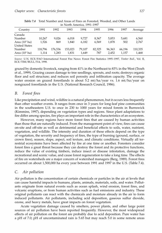
Chapter seven: Characteristic forests 127
grazed by domestic livestock, ranging from 41% in the Northeast to 83% in the West (Troehet al., 1999). Grazing causes damage to tree seedlings, sprouts, and roots; destroys organicfloor and soil structure; and reduces soil porosity and infiltration capacity. The averagewater erosion on grazed forestlands is about 5.2 mt/ha/year vs. 1.6 mt/ha/year onnongrazed forestlands in the U.S. (National Research Council, 1986).
B. Forest fires
Like precipitation and wind, wildfire is a natural phenomenon, but it occurs less frequentlythan other weather events. It ranges from once in 3 years for long-leaf pine communitiesin the southeastern U.S. to once in 230 to 1000 years for mixed forests in Burnswick(Kimmins, 1997), depending on vegetation types and regions. Since plant adaptations tofire differ among species, fire plays an important role in the characteristics of an ecosystem.
However, many regions have more forest fires that are caused by human activitiesthan those that are naturally induced. From the management point of view, fires can causeon-site and off-site as well as detrimental and beneficial effects to soils, water, nutrient,vegetation, and wildlife. The intensity and duration of these effects depend on the typeof vegetation, the severity and frequency of fires, the type of burning (ground, surface, orcrown fires), season, slope, aspect, soil texture, and climatic conditions. Virtually all ter-restrial ecosystems have been affected by fire at one time or another. Foresters considerforest fires a great threat because they can destroy the forest and its protective functions,reduce the value of existing timbers, induce insect or disease infestation, damage therecreational and scenic value, and cause forest regeneration to take a long time. The effectsof fire on watersheds are a major concern of watershed managers (Berg, 1989). Forest firesoccurred on about 1,500,000 ha every year between 1991 and 1997 in the U.S. (Table 7.4).
C. Air pollution
Air pollution is the concentration of certain chemicals or particles in the air at levels thatcan cause harmful impacts to humans, plants, animals, materials, soils, and water. Pollut-ants originate from natural events such as ocean splash, wind erosion, forest fires, andvolcanic eruptions, or from human activities such as fuel emissions and industry. Theseoriginal pollutants can react with the chemicals and moisture already in the air to forminduced pollutants. Air pollutants, including acid deposition, gaseous sulfur dioxide,ozone, and heavy metals, have great impacts on forest vegetation.
Acute vegetation damage caused by smelters, power plants, and other large pointsources of air pollution have been reported frequently. However, the most widespreadeffects of air pollution on the forest are probably due to acid deposition. Pure water hasa pH of 7.0; pH of uncontaminated rain is 5.65 but may reach 5.0 in some remote areas
Table 7.4 Total Number and Areas of Fires on Forested, Wooded, and Other Lands in North America, 1991–1997
Country 1991 1992 1993 1994 1995 1996 1997 Average
CanadaNumber 10,267 9,026 6,018 9,727 8,367 5,853 5,681 6,560Area (103 ha) 1,526 869 1,840 6,182 6,569 1,878 502 2,767United StatesNumber 118,796 176,536 153,023 79,107 82,325 96,363 66,196 110,335Area (103 ha) 1,114 1,283 1,831 1,649 787 2,452 1,157 1,468
Source: U.N. ECE/FAO International Forest Fire News: Forest Fire Statistics 1995–1997, Timber Bull., Vol. II,ECE/TIM/BULL/514, 1998.
1363_C07_fm Page 127 Wednesday, December 4, 2002 7:41 AM
128 Forest Hydrology: An Introduction to Water and Forests
of the world (Council on Environmental Quality et al., 1983). Industrial emissions such asnitrogen oxides and sulfur oxides are transformed chemically into acids with moisture inthe atmosphere and fall to the ground as acid rain, snow, and fog or dry acid-particleswith pH values lower than the reference level. In the Hubbard Brook Experimental Forest,New Hampshire, precipitation pH has been recorded as low as 3.0 (Likens et al., 1977).The acidity of pH 3.0 is 100 times greater than that of pH 5.0.
Acid deposition can adversely affect forest vegetation either directly by damagingprotective surface structures (cuticles) of the canopy or indirectly through the accelerationof soil acidification. The damage of cuticular layer can lead to malfunction of guard cells,alteration of leaf- and root-exudation processes, interference with reproduction, waterstress, and leaching of minerals from the canopy. The soil acidification can lead to leachesof basic nutrient ions, alterations of nutrient availability, slowdown of microbiologicalprocesses, reduction of microbial populations and variety, and increases in ion toxicitylevel to plants. Combining these effects on soils and plants can ultimately result in leafcoloration and abscission, and in reduction of forest growth, productivity, and speciesdiversity. The former West Germany employed a loss of tree’s foliage by 11% or more asthe main criterion in air-pollution damage inventories (Huettl, 1989).
Air pollution is a major concern in industrial countries, especially in central Europeand North America. In Europe, trees between 3.5 and 4 million ha showed injury linkedto air pollution in the early 1980s (Postel, 1984). Former West Germany estimated forestdamage by air pollution at 562,000 ha in 1982 and increased to 2,545,000 ha in 1983, or34% of the nation’s forests. The damage further increased to 50% in 1985 and 54% in fall1986, of which 19% was marked by foliage losses greater than 25% (Huettl, 1989).
In the U.S., injury and mortality of pine has been most extensive in California, of redspruce in the Appalachian Mountains, of yellow pines in the Southeast, of eastern whitepines in the East, and of sugar maples in the Northeast and Canada. Some of the damagebegan as early as in the late 1940s. In view of the complexity of the forest ecosystems,MacKenzie and El-Ashry (1989) stated that these injuries and declines probably were acollective reflection of multiple stresses, such as acid deposition, ozone, and drought,rather than of a single cause.
ReferencesBerg, N.H. (Technical Coordinator), 1989, Proceedings of the Symposium on Fire and Watershed
Management, Gen. Tech. Rep. PSW-109, U.S. Forest Service, Pacific SW Forest and RangeExp. Sta., Berkeley, CA.
Brown, S., Gillespie, A.J.R., and Lugo, A.E., 1989, Biomass estimation methods for tropical forestswith applications to forest inventory data, Forest Sci., 35, 881–902.
Brown, S. and Lugo, A.L., 1984, Biomass of tropical forests: a new estimate based on forest volumes,Science, 223, 1290–1293.
Bruijnzeel, L.A., 1996, Predicting the hydrological impacts of land cover transformation in the humidtropics: the need for integrated research, in Amazonian Deforestation and Climate, Gash, J.H.C.et al., Eds., John Wiley & Sons, New York, pp.15–55.
Buell, J. H., 1949, Trees living together: the community of trees, in Trees, Yearbook of Agri., USDA,Washington, D.C., pp. 103–108.
Burch, W.R., Jr., Alan, F., and Hermann, R.K., 1976, Forest and Future Resource Conflicts, Dept. ofPrinting, Oregon State University, Corvallis, OR.
Chang, M., et al., 1994, Air and soil temperature under three forest conditions in East Texas, TexasJ. Sci., 46, 143–155.
Chang, M., Roth, F.A., II, and Hunt, E.V., Jr., 1982, Sediment production under various forest-siteconditions, in Recent Developments in the Explanation and Prediction of Erosion and SedimentYield, Proc. of the Exeter Sym., Walling, D.E., Ed., IAHS, pp. 13–22.
1363_C07_fm Page 128 Wednesday, December 4, 2002 7:41 AM

Chapter seven: Characteristic forests 129
Council on Environmental Quality et al., 1983, National Acid Precipitation Assessment Program,Annual Report, 1983 to the President and Congress. Interagency Task Force on Acid Precip-itation, NAPAP, Washington, D.C.
Culf, A.D. et al., 1996, Radiation, temperature and humidity over forest and pasture in Amazonia,in Amazonian Deforestation and Climate, Gash, J.H.C. et al., Eds., John Wiley & Sons, NewYork,. pp. 175–191.
Davis, E.A. and Pase, C.P., 1977, Root system of shrub live oak: implications for water yield inArizona chaparral, J. Soil Water Conserv., 32, 174–180.
Department of Energy, 1992, Sector-Specific Issues and Reporting Methodologies Supporting theGeneral Guidelines for the Voluntary Reporting of the Greenhouse Gases under Section1605(b) of the Energy Policy Act of 1992.
Deurr, W.A., 1979, American forest resource management, in Forest Resource Management, Decision-Making Principles and Cases, Duerr, W.A. et al., Eds., W.B. Saunders, Philadelphia, pp. 9–20.
Dixon, R.K. et al., 1994, Carbon pools and flux of global forest ecosystems, Science, 263, 185–190.FAO, 1995, Forest Resources Assessment 1990: Global Synthesis, FAO Forestry Paper 124, Rome.Farrish, K.W., 1991, Spatial and temporal fine-root distribution in three Louisiana forest soils, Soil
Sci. Soc. Am. J., 55, 1752–1757.Fung, P.Y.H., 1982, Wood energy prospects, in Energy from Forest Biomass, Smith, W.R., Ed., Academic
Press, New York, Pp. 155–170.Gash, J.H.C. et al., Eds., 1996, Amazonian Deforestation and Climate, John Wiley & Sons, New York.Gholz, H.L., Fitz, F.K., and Waring, R.H., 1976, Lear area differences associated with old-growth
forest communities in the western Oregon Cascades, Can. J. Forest Res., 6, 49–57.Gower, S.T. and Son, Y., 1992, Differences in soil and leaf litterfall nitrogen dynamics for five forest
plantations, Soil Sci. Soc. Am. J., 56, 1959–1966.Honzák, M. et al., 1996, Estimation of leaf area index and total biomass of tropical regenerating
forests: comparison of methodologies, in Amazonian Deforestation and Climate, Gash, J.H.C. etal., Eds., John Wiley & Sons, New York.
Huettl, R.F., 1989, “New types” of forest damages in central Europe, in Air Pollution’s Toll on Forestand Crops, MacKenzie, J.J. and El-Ashry, M.T., Eds., Yale University Press, New Haven, pp.22–74.
Hughes, R.O. and Dunning, D., 1949, Pine forests of California, in U.S. Dep. of Agr., Yearbook of Agr.,Washington, D.C., pp. 352–358.
Kaufmann, M.R., Edminster, C.E., and Troendle, C.A., 1982, Leaf area determination for subalpinetree species in the Central Rocky Mountains, Res. Paper RM-238, USDA Forest Service.
Keeley, J. E. and Keeley, S.C., 1998, Chaparral, in North American Terrestrial Vegetation, Barbour, M.G.and Billings, W.D., Eds., Cambridge University Press, Cambridge, pp. 163–207.
Kimmins, J.P., 1997, Forest Ecology, A Foundation for Sustainable Management, Prentice Hall, New York.Kleinfelder, D. et al., 1992, Unconfined compressive strength of some streambank soils with herba-
ceous roots, Soil Sci. Soc. Am. J., 56, 1920–1925.Lal, J.B., 1992, Conservation and sustainable use of India’s forest resources, in Forest Ecosystems of
the World, Shafi, M. and Raza, M., Eds., Rawat Publications, New Delhi, pp. 27–35.Landsberg, H., 1968, Physical Climatology, Gray Printing Co., DuBois, PA.Lanly, J-P., Singh, K.D., and Janz, K., 1991, FAO’s 1990 reassessment of tropical forest cover, Nature
Resour., 27, 21–26.Likens, G.E. et al., 1977, Biogeochemistry, Springer-Verlag, Heidelberg.Lugo, A.E. and Brown, S., 1992, Tropical forests as sinks of atmospheric carbon, Forest Ecol. Manage.,
54. 239–255.MacCleery, D.W., 1993, American Forests, a History of Resiliency and Recovery, FS-540, USDA-Forest
Service.MacKenzie, J.J. and El-Ashry, M.T., 1989, Tree and crop injury: a summary of the evidence, in Air
Pollution’s Toll on Forest and Crops, MacKenzie, J.J. and El-Ashry, M.T., Eds., Yale UniversityPress, New Haven, pp. 1–21.
Mader, S.S., 1998. Biology, McGraw-Hill, New York.Mather, A.S., 1990, Global Forest Resources, Timber Press, Portland, OR.
1363_C07_fm Page 129 Wednesday, December 4, 2002 7:41 AM

130 Forest Hydrology: An Introduction to Water and Forests
Medina, E. and Cuevas, E., 1997, Biomass production and accumulation in nutrient-limited rainforests: implications for responses to global change, in Amazonian Deforestation and Climate,Gash, J.H.C. et al., Eds., John Wiley & Sons, New York, pp. 221–239.
Miller, G.T., Jr., 1999, Environmental Science, Working with the Earth, Wadsworth, New York.Mirov, N.T., 1949, A tree is a living thing, in Trees, Yearbook of Agr., USDA, Washington, D.C., pp. 1–10.National Audubon Society, Inc., 1992, The Audubon Society Field Guide to North American Trees, Alfred
A. Knopf, New York.National Research Council, 1986, Soil Conservation: Assessing the National Resources Inventory, Vol. 1,
p.7.Natural Resources Conservation Service, 1999, Summary Report: 1997 National Resources Inventory,
USDA, Washington, D.C.Peet, R.K., 1988, Forests of the rocky mountains, in North American Terrestrial Vegetation, Barbour,
M.G. and Billings, W.D., Eds., Cambridge University Press, Cambridge. pp. 63–101.Perry, D.A., 1994, Forest Ecosystems, Johns Hopkins University Press, Baltimore.Phillips, W.S., 1963, Depth of roots in soil, Ecology, 44, 424.Postel, S., 1984, Air Pollution, Acid Rain, and the Future of Forests, Worldwatch Paper 58, World-
watch Institute, Washington, D.C.Reifsnyder, W.E. and Lull, H.W., 1965, Radiant Energy in Relation to Forests, Tech. Bull. No. 1344,
USDA Forest Service.Shafi, M., 1992, Utilization and conservation of forests in India with special reference to social
forestry, in Forest Ecosystems of the World, Shafi, M. and Raza, M., Eds., Rawat Publications,New Delhi, pp. 21–26.
Sidle, R.C., Pearce, A.J., and O’Loughlin, C.L., 1985, Hillslope Stability and Land Use, Water Resour.Monograph Series 11, Amer. Geophy. Union, Washington, D.C.
Spurr, S.H. and Barnes, B.V., 1973, Forest Ecology, 2nd ed., Ronald, New York.Stout, B.B., 1956, Studies of the Root Systems of Deciduous Trees, Black Rock Forest Bull. No. 15,
Harvest University.Sutton, O.G., 1953, Micrometeorology, McGraw-Hill, New York.Swank, W.T. and Schreuder, H.T., 1974, Comparison of three methods of estimating surface and
biomass for a forest of young eastern white pine, Forest Sci, 20, 91–100.Swerdlow, J.L., 2000, Medicines in nature, Nat. Geogr., April 2000, pp.98–117.Troeh, F.R., Hobbs, J.A., and Donahue, R.L., 1999, Soil and Water Conservation: Productivity and
Environmental Protection, Prentice Hall, New York.Van Eimern, J. et al., 1964, Windbreaks and Shelterbelts, WMO Tech. Note No. 59.Waldron, L.J., and Dakessian, S., 1982, Effects of grass, legumes, and tree roots on soil shearing
resistance, Soil Sci. Soc. Am. J., 46, 894–899.WMO (World Meteorological Organization), 1964, Windbreaks and Shelterbelts, WMO-No.
147.TP.70. Tech. Note No. 59. Geneva, Switzerland.WMO, 1981, Meteorological Aspects of the Utilization of Wind as an Energy Source, WMO-NO.575,
Tech. Note No. 175. Geneva, Switzerland.World Resources Institute, the U.N. Environmental Programme, the U.N. Development Programme,
and the World Bank, 1996, World Resources, 1996–97, Oxford University Press, Oxford.
1363_C07_fm Page 130 Wednesday, December 4, 2002 7:41 AM
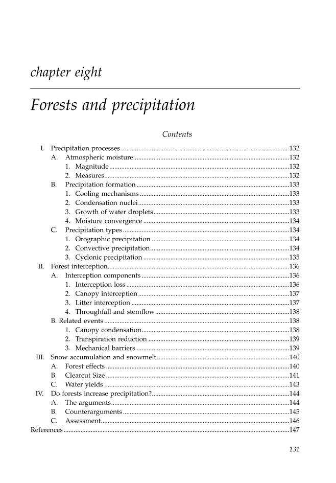
131
chapter eight
Forests and precipitation
Contents
I. Precipitation processes ...................................................................................................132A. Atmospheric moisture............................................................................................132
1. Magnitude..........................................................................................................1322. Measures.............................................................................................................132
B. Precipitation formation ..........................................................................................1331. Cooling mechanisms ........................................................................................1332. Condensation nuclei.........................................................................................1333. Growth of water droplets................................................................................1334. Moisture convergence ......................................................................................134
C. Precipitation types ..................................................................................................1341. Orographic precipitation .................................................................................1342. Convective precipitation..................................................................................1343. Cyclonic precipitation ......................................................................................135
II. Forest interception...........................................................................................................136A. Interception components .......................................................................................136
1. Interception loss ................................................................................................1362. Canopy interception .........................................................................................1373. Litter interception .............................................................................................1374. Throughfall and stemflow...............................................................................138
B. Related events .............................................................................................................1381. Canopy condensation.......................................................................................1382. Transpiration reduction ...................................................................................1393. Mechanical barriers ..........................................................................................139
III. Snow accumulation and snowmelt ..............................................................................140A. Forest effects ............................................................................................................140B. Clearcut Size ............................................................................................................141C. Water yields .............................................................................................................143
IV. Do forests increase precipitation?.................................................................................144A. The arguments.........................................................................................................144B. Counterarguments ..................................................................................................145C. Assessment...............................................................................................................146
References .....................................................................................................................................147
1363_C08_fm Page 131 Wednesday, December 4, 2002 7:42 AM
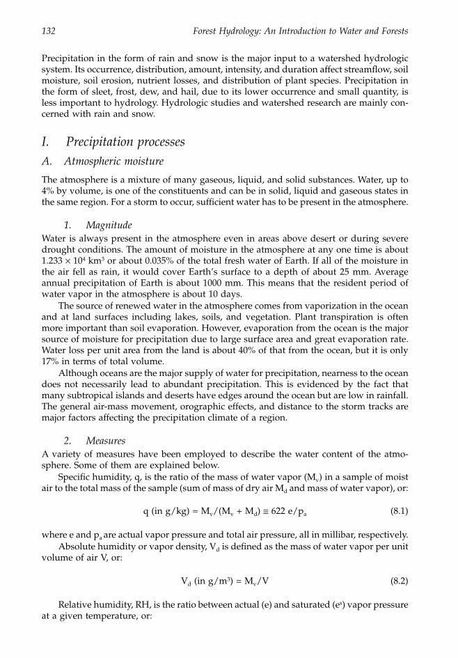
132 Forest Hydrology: An Introduction to Water and Forests
Precipitation in the form of rain and snow is the major input to a watershed hydrologicsystem. Its occurrence, distribution, amount, intensity, and duration affect streamflow, soilmoisture, soil erosion, nutrient losses, and distribution of plant species. Precipitation inthe form of sleet, frost, dew, and hail, due to its lower occurrence and small quantity, isless important to hydrology. Hydrologic studies and watershed research are mainly con-cerned with rain and snow.
I. Precipitation processes
A. Atmospheric moisture
The atmosphere is a mixture of many gaseous, liquid, and solid substances. Water, up to4% by volume, is one of the constituents and can be in solid, liquid and gaseous states inthe same region. For a storm to occur, sufficient water has to be present in the atmosphere.
1. Magnitude
Water is always present in the atmosphere even in areas above desert or during severedrought conditions. The amount of moisture in the atmosphere at any one time is about1.233
¥
10
4
km
3
or about 0.035% of the total fresh water of Earth. If all of the moisture inthe air fell as rain, it would cover Earth’s surface to a depth of about 25 mm. Averageannual precipitation of Earth is about 1000 mm. This means that the resident period ofwater vapor in the atmosphere is about 10 days.
The source of renewed water in the atmosphere comes from vaporization in the oceanand at land surfaces including lakes, soils, and vegetation. Plant transpiration is oftenmore important than soil evaporation. However, evaporation from the ocean is the majorsource of moisture for precipitation due to large surface area and great evaporation rate.Water loss per unit area from the land is about 40% of that from the ocean, but it is only17% in terms of total volume.
Although oceans are the major supply of water for precipitation, nearness to the oceandoes not necessarily lead to abundant precipitation. This is evidenced by the fact thatmany subtropical islands and deserts have edges around the ocean but are low in rainfall.The general air-mass movement, orographic effects, and distance to the storm tracks aremajor factors affecting the precipitation climate of a region.
2. Measures
A variety of measures have been employed to describe the water content of the atmo-sphere. Some of them are explained below.
Specific humidity, q, is the ratio of the mass of water vapor (M
v
) in a sample of moistair to the total mass of the sample (sum of mass of dry air M
d
and mass of water vapor), or:
q (in g/kg) = M
v
/(M
v
+ M
d
)
@
622 e/p
a
(8.1)
where e and p
a
are actual vapor pressure and total air pressure, all in millibar, respectively.Absolute humidity or vapor density, V
d
is defined as the mass of water vapor per unitvolume of air V, or:
V
d
(in g/m
3
) = M
v
/V (8.2)
Relative humidity, RH, is the ratio between actual (e) and saturated (e
s
) vapor pressureat a given temperature, or:
1363_C08_fm Page 132 Wednesday, December 4, 2002 7:42 AM
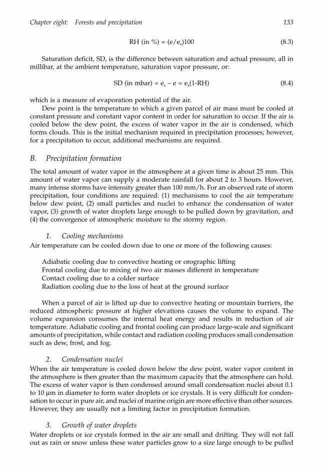
Chapter eight: Forests and precipitation 133
RH (in %) = (e/e
s
)100 (8.3)
Saturation deficit, SD, is the difference between saturation and actual pressure, all inmillibar, at the ambient temperature, saturation vapor pressure, or:
SD (in mbar) = e
s
– e = e
s
(1-RH) (8.4)
which is a measure of evaporation potential of the air.Dew point is the temperature to which a given parcel of air mass must be cooled at
constant pressure and constant vapor content in order for saturation to occur. If the air iscooled below the dew point, the excess of water vapor in the air is condensed, whichforms clouds. This is the initial mechanism required in precipitation processes; however,for a precipitation to occur, additional mechanisms are required.
B. Precipitation formation
The total amount of water vapor in the atmosphere at a given time is about 25 mm. Thisamount of water vapor can supply a moderate rainfall for about 2 to 3 hours. However,many intense storms have intensity greater than 100 mm/h. For an observed rate of stormprecipitation, four conditions are required: (1) mechanisms to cool the air temperaturebelow dew point, (2) small particles and nuclei to enhance the condensation of watervapor, (3) growth of water droplets large enough to be pulled down by gravitation, and(4) the convergence of atmospheric moisture to the stormy region.
1. Cooling mechanisms
Air temperature can be cooled down due to one or more of the following causes:
Adiabatic cooling due to convective heating or orographic liftingFrontal cooling due to mixing of two air masses different in temperatureContact cooling due to a colder surfaceRadiation cooling due to the loss of heat at the ground surface
When a parcel of air is lifted up due to convective heating or mountain barriers, thereduced atmospheric pressure at higher elevations causes the volume to expand. Thevolume expansion consumes the internal heat energy and results in reduction of airtemperature. Adiabatic cooling and frontal cooling can produce large-scale and significantamounts of precipitation, while contact and radiation cooling produces small condensationsuch as dew, frost, and fog.
2. Condensation nuclei
When the air temperature is cooled down below the dew point, water vapor content inthe atmosphere is then greater than the maximum capacity that the atmosphere can hold.The excess of water vapor is then condensed around small condensation nuclei about 0.1to 10
m
m in diameter to form water droplets or ice crystals. It is very difficult for conden-sation to occur in pure air, and nuclei of marine origin are more effective than other sources.However, they are usually not a limiting factor in precipitation formation.
3. Growth of water droplets
Water droplets or ice crystals formed in the air are small and drifting. They will not fallout as rain or snow unless these water particles grow to a size large enough to be pulled
1363_C08_fm Page 133 Wednesday, December 4, 2002 7:42 AM
134 Forest Hydrology: An Introduction to Water and Forests
down by gravitation. The growth of these particles may be due to collisions with oneanother when they drift in the air. They can grow at the expense of other particles due toevaporation and condensation because saturation vapor pressure can be different amongwater droplets and ice crystals. This process is called coalescence.
4. Moisture convergence
Water-vapor content in the atmosphere is about 25 mm at any given time. Thus, additionalwater must be supplied from the surrounding areas dominated with high pressure to thestormy areas dominated with low pressure in order for a storm to remain at a constantrate or even increase during a storm system. The greater the atmospheric pressure gradientbetween the high and low pressure areas, the greater the storm intensity.
C. Precipitation types
Precipitation is often categorized into three types in accordance with cooling mechanismsthat generate vertical lifting and formation of precipitation.
1. Orographic precipitation
When an air mass is lifted up mechanically by mountain barriers, the reduced atmosphericpressure at higher elevations causes cooling and condensation by expansion. It results ingreater precipitation (Figure 8.1). Thus, precipitation is greater at higher elevations on thewindward slope of mountainous areas. The increasing rate, the so-called precipitationgradient, ranges from 12 to 165 mm/100 m in the coastal range of Washington to5 mm/100 m in western Colorado. However, there is an upper limit on the increase inprecipitation with elevation. The zone of maximum precipitation is about 2135 m at theAlps, 1525 m in northern California, and 2440 m in the southern Sierra Nevada. Beyondthis level, precipitation decreases.
2. Convective precipitation
Unequal heating between different surfaces, such as plowed field vs. forest or land vs.water, or the increase of water vapor content in the air due to evapotranspiration in hot
Figure 8.1
Orographic effects on precipitation in Washington state. (After Small, R.T., 1966, Weath-erwise, October, 204–207.)
10,000 ft � 15.0°F � 15.0°F � 20.8 in�(3,048 m) (-9.4°C) (-9.4°C) (52.8 cm)
6,000 ft � 28.2°F � 28.2°F � 24.28 in�(1,829 m) (-2.1°C) (-2.1°C) (61.7 cm)
3,000 ft � 44.1°F � 31.7°F � 26.60 in�(914 m) (6.7°C) (-0.2°C) (67.6 cm)
(Relative Humdity = 39%)�Surface � 60.0°F � 35.0°F � 30.00 in� (15.6°C) (1.7°C) (76.2 cm)
Dry rate = 5.3°F/1000 ft, or 1.0°C/100 m�Moist rate = 5.3°F/1000 ft, or 1.0°C/100 m�Dewpoint rate = 5.3°F/1000 ft, or 1.0°C/100 m�Condensation height, ft = 1000(T-D)/4.2 (in British units)�Condensation height, m = 100(T-D)/0.7655 (in metric units)
15.5°F � 15.5°F �(-9.4°C) (-9.4°C)
36.2°F � 19.4°F �(2.3°C) (-7.0°C)
52.1°F � 22.7°F �(11.2°C) (-5.2°C)
RH = 20%�68.0°F � 26.0°F �(20.0°C) (-3.3°C)
E = Elevation, T = Air Temperature�D = Dewpoint, P = Pressure
E T D P T D
1363_C08_fm Page 134 Wednesday, December 4, 2002 7:42 AM
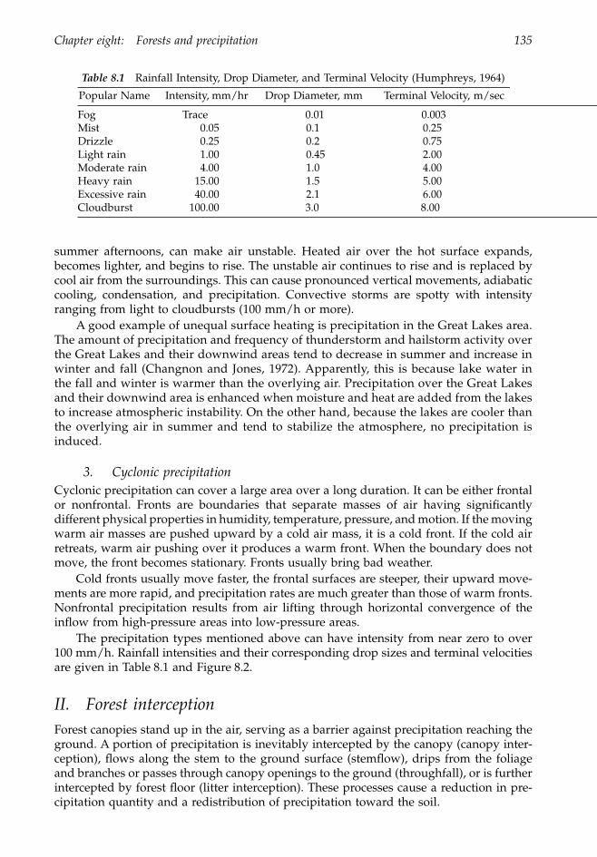
Chapter eight: Forests and precipitation 135
summer afternoons, can make air unstable. Heated air over the hot surface expands,becomes lighter, and begins to rise. The unstable air continues to rise and is replaced bycool air from the surroundings. This can cause pronounced vertical movements, adiabaticcooling, condensation, and precipitation. Convective storms are spotty with intensityranging from light to cloudbursts (100 mm/h or more).
A good example of unequal surface heating is precipitation in the Great Lakes area.The amount of precipitation and frequency of thunderstorm and hailstorm activity overthe Great Lakes and their downwind areas tend to decrease in summer and increase inwinter and fall (Changnon and Jones, 1972). Apparently, this is because lake water inthe fall and winter is warmer than the overlying air. Precipitation over the Great Lakesand their downwind area is enhanced when moisture and heat are added from the lakesto increase atmospheric instability. On the other hand, because the lakes are cooler thanthe overlying air in summer and tend to stabilize the atmosphere, no precipitation isinduced.
3. Cyclonic precipitation
Cyclonic precipitation can cover a large area over a long duration. It can be either frontalor nonfrontal. Fronts are boundaries that separate masses of air having significantlydifferent physical properties in humidity, temperature, pressure, and motion. If the movingwarm air masses are pushed upward by a cold air mass, it is a cold front. If the cold airretreats, warm air pushing over it produces a warm front. When the boundary does notmove, the front becomes stationary. Fronts usually bring bad weather.
Cold fronts usually move faster, the frontal surfaces are steeper, their upward move-ments are more rapid, and precipitation rates are much greater than those of warm fronts.Nonfrontal precipitation results from air lifting through horizontal convergence of theinflow from high-pressure areas into low-pressure areas.
The precipitation types mentioned above can have intensity from near zero to over100 mm/h. Rainfall intensities and their corresponding drop sizes and terminal velocitiesare given in Table 8.1 and Figure 8.2.
II. Forest interception
Forest canopies stand up in the air, serving as a barrier against precipitation reaching theground. A portion of precipitation is inevitably intercepted by the canopy (canopy inter-ception), flows along the stem to the ground surface (stemflow), drips from the foliageand branches or passes through canopy openings to the ground (throughfall), or is furtherintercepted by forest floor (litter interception). These processes cause a reduction in pre-cipitation quantity and a redistribution of precipitation toward the soil.
Table 8.1
Rainfall Intensity, Drop Diameter, and Terminal Velocity (Humphreys, 1964)
Popular Name Intensity, mm/hr Drop Diameter, mm Terminal Velocity, m/sec
Fog Trace 0.01 0.003Mist 0.05 0.1 0.25Drizzle 0.25 0.2 0.75Light rain 1.00 0.45 2.00Moderate rain 4.00 1.0 4.00Heavy rain 15.00 1.5 5.00Excessive rain 40.00 2.1 6.00Cloudburst 100.00 3.0 8.00
1363_C08_fm Page 135 Wednesday, December 4, 2002 7:42 AM
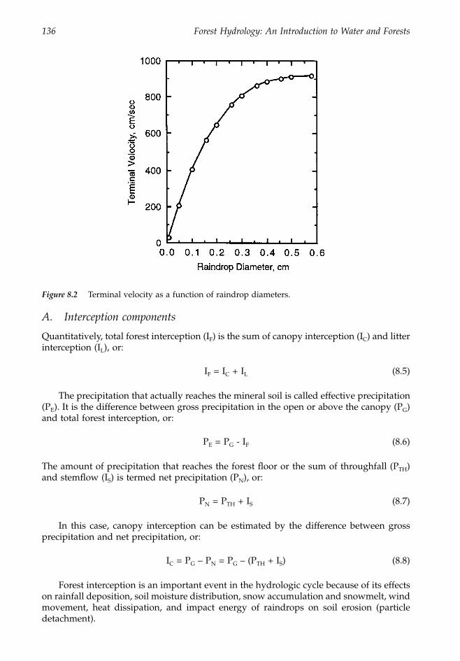
136 Forest Hydrology: An Introduction to Water and Forests
A. Interception components
Quantitatively, total forest interception (I
F
) is the sum of canopy interception (I
C
) and litterinterception (I
L
), or:
I
F
= I
C
+ I
L
(8.5)
The precipitation that actually reaches the mineral soil is called effective precipitation(P
E
). It is the difference between gross precipitation in the open or above the canopy (P
G
)and total forest interception, or:
P
E
= P
G
- I
F
(8.6)
The amount of precipitation that reaches the forest floor or the sum of throughfall (P
TH
)and stemflow (I
S
) is termed net precipitation (P
N
), or:
P
N
= P
TH
+ I
S
(8.7)
In this case, canopy interception can be estimated by the difference between grossprecipitation and net precipitation, or:
I
C
= P
G
– P
N
= P
G
– (P
TH
+ I
S
) (8.8)
Forest interception is an important event in the hydrologic cycle because of its effectson rainfall deposition, soil moisture distribution, snow accumulation and snowmelt, windmovement, heat dissipation, and impact energy of raindrops on soil erosion (particledetachment).
Figure 8.2
Terminal velocity as a function of raindrop diameters.
1363_C08_fm Page 136 Wednesday, December 4, 2002 7:42 AM
Chapter eight: Forests and precipitation 137
1. Interception loss
Precipitation intercepted by forest canopies and litter floor, collectively termed forestinterception, is lost to the air by evaporation. It is a negative term in the hydrologic budget.For eastern white pine stands 10, 35, and 60 years old in western North Carolina, Helvey(1967) showed that total interception loss increased with maturity and could be estimatedempirically from gross precipitation for a given season (P
G
) and number of storms (N) inthat season:
I
F
= 1.27N + 0.08 P
G
(for 10 years stand) (8.9)
I
F
= 1.27N + 0.12 P
G
(for 35 years stand)
I
F
= 1.52N + 0.18 P
G
(for 60 years stand)
2. Canopy interception
Approximately 10 to 20% of annual precipitation is lost by canopy interception, dependingon evaporation power of the air, storm characteristics, and vegetation. In field observa-tions, canopy interception is frequently expressed in this empirical form:
I
C
= a + b P
G
(8.10)
where a and b are regression coefficients. However, a can be considered the canopy storage,which is the amount of water retained on the canopy when rainfall and throughfall haveceased, and b is equivalent to the average evaporation rate of the intercepted water duringrainfall.
During the beginning of a storm, water storage in the canopy increases with time andgradually levels off at maximum canopy storage capacity as storm duration is prolongedor intensity increases. The canopy storage is affected by factors such as leaf quantity,orientation, and surface features. Satterlund and Adams (1992) state that temperature alsohas effects on the storage capacity through its modification of water viscosity and surfacetension. This effect may be too small to be significant or within a magnitude less thanmeasurement errors.
The quantity of leaves varies among species and among forest stands. It is commonlyexpressed in terms of leaf area index, the ratio of total surface area of vegetation to thecovered areas in m
2
/m
2
. The leaf area index ranges from 0.5 to 4.5 for sugarcane in Florida(Shih, 1989), 5.3 for a 10-year-old stand of eastern white pine (Swank and Schreuder, 1974),10.2 for Norway spruce in Wisconsin (Gower and Son, 1992), and 40 to 50 for a maturestand of 90% spruce and 10% fir in the central Rocky Mountains (Kaufmann et al., 1982).Generally, the tall, mature, and evergreen conifer species are the greatest, followed bydeciduous hardwoods, shrubs, forbs, and grasses. Thus, the capacity of canopy storageamong vegetation should also reflect this order. An extensive review in the Americanliterature showed that the storage capacity ranges from 0.3 to 6.6 mm for conifers, 0.03 to2.0 mm for hardwoods, 0.3 to 2.0 for shrubs, and 1.0 to 1.5 mm for grasses (Zinke, 1967).
From a review of forest-interception studies in North America (Helvey, 1971), the bvalues can be derived as 0.21 for spruce–fir–hemlock (i.e., 21% of gross precipitation), 0.11for red pine, 0.07 for ponderosa pine, and 0.06 and 0.03 for the growing and dormantseason of mature mixed hardwoods, respectively. These are approximate values becausethey are used to apply to all gross precipitation, regardless of intensity and duration, andthe interval between storms. In addition, they should not be extrapolated to forests andclimatic conditions from which the b values were not derived.
1363_C08_fm Page 137 Wednesday, December 4, 2002 7:42 AM
138 Forest Hydrology: An Introduction to Water and Forests
Actually, evaporation of canopy-intercepted water should be determined by availableenergy, vapor pressure gradient, aerodynamic resistance of the leaves, and air character-istics. When the whole canopy is wet, the Monteith-Penman equation (Monteith andUnsworth, 1990) can be used to estimate the potential evaporation rate of the interceptedwater. If the canopy moisture level is less than saturation, then the potential evaporationis only proportional to the percentage of wet canopy (Rutter and Morton, 1977). Physicalor analytical models for estimating evaporation of canopy-intercepted water are availablefrom Rutter et al. (1975), Stewart (1977), and Gash (1979). These models require hourlyinputs of meteorological data, which are not available in most forested areas.
3. Litter interception
Litter interception is much smaller than canopy interception. The amount is largelydependent upon the thickness of litter, water-holding capacity, the frequency of wetting,and evaporation rate. Studies have shown that it is only a few millimeters in depth inmost cases and can be up to 11 mm during a storm. Generally, about 1 to 5% of annualprecipitation (Helvey and Patric, 1965) and less than 50 mm/year are lost to litterinterception. However, it has been reported to be as high as 17% of gross precipitationunder pole size (30 to 70 years) ponderosa pine stands (Alden, 1968) and 94 mm/yearfor shortleaf pine (Rusk, 1969).
Although litter reduces the quantity of precipitation actually reaching the mineral soil,most importantly it also affects the velocity of overland flow, which allows more time forsoils to absorb runoff water. It also protects the ground surface from direct impact ofraindrop energy and wind energy as well as shades the soil surface, which in turn canreduce soil evaporation. Thus, the conservation of soil moisture due to evaporation reduc-tion for a period of time can outweigh litter interception of the forest floor. Runoff andsediment production in areas covered by litter is much lower than in areas with no coverof litter (Singer and Blackard, 1978).
Unger and Parker (1976) showed that a 1-cm thick floor of crop litter can reducepotential evaporation to 46% and can further reduce to about 17% and 6% if the litter flooris increased to 3 and 5 cm in depth, respectively. A litter floor of 3 cm is common in foreststands. The soil moisture conservation of a 3-cm litter floor in a 5-day period can reach20 mm of water, much greater than the 1 to 5% of rainfall that can be lost due to litterinterception in one or two storms.
4. Throughfall and stemflow
The total of throughfall and stemflow, termed net precipitation, is subject to litter inter-ception before reaching the mineral soil. Throughfall is highly variable among forests andwithin a forest. Drips from certain points in a stand can cause more throughfall than thetotal rainfall in the open. Average throughfall of a stand is determined by factors such asspecies, age, density, season, and storm characteristics. For example, total throughfall wasabout 88, 85, 83, and 82% of gross precipitation for four adjacent longleaf, loblolly, slash,and shortleaf pine stands in east Texas (Roth and Chang, 1981), different by 5% from thoseweighted values proposed by Helvey (1971) (Table 8.2).
The greatest amount of stemflow reported in the literature is 12% of gross precipi-tation in a loblolly pine stand in South Carolina (Swank et al., 1972). This may be dueto the sharp angles between branches and trunks. For most species, about 2 to 5% ofgross precipitation flows to the ground along stems. Although it is small in quantity, itmay be of ecological importance because rainwater flows directly into the rooting zoneof the tree.
1363_C08_fm Page 138 Wednesday, December 4, 2002 7:42 AM
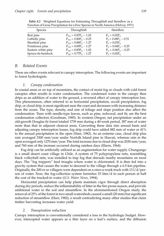
Chapter eight: Forests and precipitation 139
B. Related Events
There are other events relevant to canopy interception. The following events are importantto forest hydrologists.
1. Canopy condensation
In coastal areas or on top of mountains, the contact of moist fog or clouds with cold forestcanopies often results in water condensation. The condensed water in the canopy thendrips as an addition of water to the ground, a reversed effect of canopy interception loss.This phenomenon, often referred to as horizontal precipitation, occult precipitation, fogdrip, or cloud drip, is most significant near the coast and decreases with increasing distancefrom the ocean. The type, density, and size of foliage and slope position also affect thecondensation. Trees with needle-type leaves, such as pine, redwood, and fir, are the bestcondensation collectors (Goodman, 1985). In western Oregon, net precipitation under anold-growth Douglas fir forest totaled 1739 mm during a 40-week period, 387 mm of watermore than that in adjacent clearcut areas. Converting these data into annual basis andadjusting canopy interception losses, fog drip could have added 882 mm of water or 41%to the annual precipitation in the open (Harr, 1982). As an extreme case, cloud drip plusrain averaged 3300 mm/year under Norfolk Island pine in Hawaii, whereas rain in theopen averaged only 1270 mm/year. The total increase due to cloud drip was 2030 mm/year,and 760 mm of the increase occurred during rainless days (Ekern, 1964).
Fog drip can be artificially utilized as an augmentation for water supply. Chungungois a small desert coast village in Chile. A system of 75 polypropylene nets, resemblingblack volleyball nets, was installed to trap fog that shrouds nearby mountains on mostdays. The “fog trappers” feed troughs where water is chlorinated. It is then fed into agravity system that causes the water to descend to the village through a 6.5-km pipeline.Originally, the 200 or so villagers were dependent on a once-a-week truck with 13 l/d/per-son of water. Now, the fog-collection system furnishes 53 liter/d to each person at halfthe cost of the trucked-in water (
U.S. Water News
, 1994).Horizontal precipitation can help plants maintain vigor through direct absorption
during dry periods, reduce the inflammability of litter in the fire-prone season, and provideadditional water to the soil and streamflow. In the aforementioned Oregon study, theremoval of 25% of the forest in two small watersheds caused a small (20 mm) but significantreduction of streamflow (Harr, 1982), a result contradicting many other studies that claimtimber harvesting increases water yield.
2. Transpiration reduction
Canopy interception is conventionally considered a loss in the hydrologic budget. How-ever, intercepted water appears as a thin layer on a leaf’s surface, and the diffusion
Table 8.2
Weighted Equations for Estimating Throughfall and Stemflow as a
Function of Gross Precipitation for a Few Species in North America (Helvey, 1971)
Species Throughfall Stemflow
Red pine P
TH
= 0.87P
G
– 1.02 P
S
= 0.02P
G
Loblolly pine P
TH
= 0.80P
G
– 0.25 P
S
= 0.08P
G
– 0.51Shortleaf pine P
TH
= 0.88P
G
– 1.27 P
S
= 0.03P
G
Pondersoa pine P
TH
= 0.89P
G
– 1.27 P
S
= 0.04P
G
– 0.25Eastern white pine P
TH
= 0.85P
G
– 1.02 P
S
= 0.06P
G
– 0.25Spruce-fir-hemlock P
TH
= 0.77P
G
– 1.27 P
S
= 0.02P
G
1363_C08_fm Page 139 Wednesday, December 4, 2002 7:42 AM
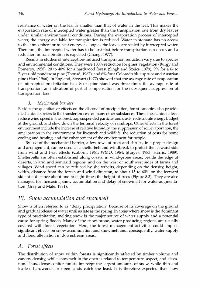
140 Forest Hydrology: An Introduction to Water and Forests
resistance of water on the leaf is smaller than that of water in the leaf. This makes theevaporation rate of intercepted water greater than the transpiration rate from dry leavesunder similar environmental conditions. During the evaporation process of interceptedwater, the energy available for transpiration is reduced. Water in stomata has no accessto the atmosphere or to heat energy as long as the leaves are sealed by intercepted water.Therefore, the intercepted water has to be lost first before transpiration can occur, and areduction in transpiration is expected (Chang, 1977).
Results in studies of interception-induced transpiration reduction vary due to speciesand environmental conditions. They were 100% reduction for grass vegetation (Burgy andPomeroy, 1958), 20 to 40% for a hardwood forest (Singh and Szeics, 1979), 9% for a 6- to7-year-old ponderosa pine (Thorud, 1967), and 6% for a Colorado blue spruce and Austrianpine (Harr, 1966). In England, Stewart (1977) showed that the average rate of evaporationof intercepted precipitation in a Scots pine stand was three times the average rate oftranspiration, an indication of partial compensation for the subsequent suppression oftranspiration loss.
3. Mechanical barriers
Besides the quantitative effects on the disposal of precipitation, forest canopies also providemechanical barriers to the transfer process of many other substances. These mechanical effectsreduce wind speed in the forest, trap suspended particles and dusts, redistribute energy budgetat the ground, and slow down the terminal velocity of raindrops. Other effects in the forestenvironment include the increase of relative humidity, the suppression of soil evaporation, theamelioration in the environment for livestock and wildlife, the reduction of costs for homecooling and heating, and the enhancement of the environment for people.
By use of the mechanical barrier, a few rows of trees and shrubs, in a proper designand arrangement, can be used as a shelterbelt and windbreak to protect the leeward sidefrom wind and heat effects (Caborn, 1964; WMO, 1964; Sturges, 1983; Harris, 1989).Shelterbelts are often established along coasts, in wind-prone areas, beside the edge ofdeserts, in arid and semiarid regions, and on the west or southwest sides of farms andvillages. Wind speed can be reduced by shelterbelts, depending on the density, height,width, distance from the forest, and wind direction, to about 15 to 60% on the leewardside at a distance about one to eight times the height of trees (Figure 8.3). They are alsomanaged for increasing snow accumulation and delay of snowmelt for water augmenta-tion (Gray and Male, 1981).
III. Snow accumulation and snowmelt
Snow is often referred to as “delay precipitation” because of its coverage on the groundand gradual release of water until as late as the spring. In areas where snow is the dominanttype of precipitation, melting snow is the major source of water supply and a potentialcause for spring floods. Many of the snow-prone, water-producing regions are usuallycovered with forest vegetation. Here, the forest management activities could imposesignificant effects on snow accumulation and snowmelt and, consequently, water supplyand flood alleviation in downstream areas.
A. Forest effects
The distribution of snow within forests is significantly affected by timber volume andcanopy density, while snowmelt in the open is related to temperature, aspect, and eleva-tion. Thus, dense conifer forests intercept the largest amounts of snow, while thin andleafless hardwoods or open lands catch the least. It is therefore expected that snow
1363_C08_fm Page 140 Wednesday, December 4, 2002 7:42 AM
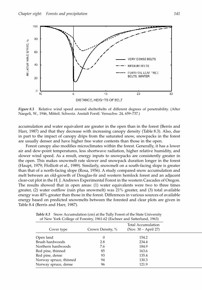
Chapter eight: Forests and precipitation 141
accumulation and water equivalent are greater in the open than in the forest (Berris andHarr, 1987) and that they decrease with increasing canopy density (Table 8.3). Also, duein part to the impact of canopy drips from the saturated snow, snowpacks in the forestare usually denser and have higher free water contents than those in the open.
Forest canopy also modifies microclimates within the forest. Generally, it has a lowerair and dew-point temperatures, less shortwave radiation, higher relative humidity, andslower wind speed. As a result, energy inputs to snowpacks are consistently greater inthe open. This makes snowmelt rate slower and snowpack duration longer in the forest(Haupt, 1979; Ffolliott et al., 1989). Similarly, snowmelt on a south-facing slope is greaterthan that of a north-facing slope (Rosa, 1956). A study compared snow accumulation andmelt between an old-growth of Douglas-fir and western hemlock forest and an adjacentclear-cut plot in the H. J. Andrews Experimental Forest in the western Cascades of Oregon.The results showed that in open areas: (1) water equivalents were two to three timesgreater, (2) water outflow (rain plus snowmelt) was 21% greater, and (3) total availableenergy was 40% greater than those in the forest. Differences in various sources of availableenergy based on predicted snowmelts between the forested and clear plots are given inTable 8.4 (Berris and Harr, 1987).
Figure 8.3
Relative wind speed around shelterbelts of different degrees of penetrability. (AfterNaegeli, W., 1946, Mitteil. Schweiz. Anstalt Forstl. Versuchw. 24, 659–737.)
Table 8.3
Snow Accumulation (cm) at the Tully Forest of the State University
of New York College of Forestry, 1961-62 (Eschner and Satterlund, 1963)
Cover type Crown Density, %Total Accumulation(Nov. 30 – April 27)
Open land 0 154.2Brush hardwoods 2.8 234.4Northern hardwoods 7.6 184.9Red pine, thinned 85 163.6Red pine, dense 93 135.4Norway spruce, thinned 94 130.3Norway spruce, dense 96 121.9
1363_C08_fm Page 141 Wednesday, December 4, 2002 7:42 AM
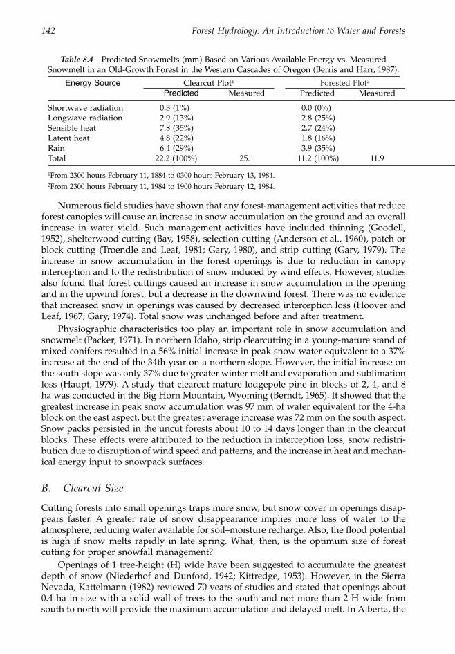
142 Forest Hydrology: An Introduction to Water and Forests
Numerous field studies have shown that any forest-management activities that reduceforest canopies will cause an increase in snow accumulation on the ground and an overallincrease in water yield. Such management activities have included thinning (Goodell,1952), shelterwood cutting (Bay, 1958), selection cutting (Anderson et al., 1960), patch orblock cutting (Troendle and Leaf, 1981; Gary, 1980), and strip cutting (Gary, 1979). Theincrease in snow accumulation in the forest openings is due to reduction in canopyinterception and to the redistribution of snow induced by wind effects. However, studiesalso found that forest cuttings caused an increase in snow accumulation in the openingand in the upwind forest, but a decrease in the downwind forest. There was no evidencethat increased snow in openings was caused by decreased interception loss (Hoover andLeaf, 1967; Gary, 1974). Total snow was unchanged before and after treatment.
Physiographic characteristics too play an important role in snow accumulation andsnowmelt (Packer, 1971). In northern Idaho, strip clearcutting in a young-mature stand ofmixed conifers resulted in a 56% initial increase in peak snow water equivalent to a 37%increase at the end of the 34th year on a northern slope. However, the initial increase onthe south slope was only 37% due to greater winter melt and evaporation and sublimationloss (Haupt, 1979). A study that clearcut mature lodgepole pine in blocks of 2, 4, and 8ha was conducted in the Big Horn Mountain, Wyoming (Berndt, 1965). It showed that thegreatest increase in peak snow accumulation was 97 mm of water equivalent for the 4-hablock on the east aspect, but the greatest average increase was 72 mm on the south aspect.Snow packs persisted in the uncut forests about 10 to 14 days longer than in the clearcutblocks. These effects were attributed to the reduction in interception loss, snow redistri-bution due to disruption of wind speed and patterns, and the increase in heat and mechan-ical energy input to snowpack surfaces.
B. Clearcut Size
Cutting forests into small openings traps more snow, but snow cover in openings disap-pears faster. A greater rate of snow disappearance implies more loss of water to theatmosphere, reducing water available for soil–moisture recharge. Also, the flood potentialis high if snow melts rapidly in late spring. What, then, is the optimum size of forestcutting for proper snowfall management?
Openings of 1 tree-height (H) wide have been suggested to accumulate the greatestdepth of snow (Niederhof and Dunford, 1942; Kittredge, 1953). However, in the SierraNevada, Kattelmann (1982) reviewed 70 years of studies and stated that openings about0.4 ha in size with a solid wall of trees to the south and not more than 2 H wide fromsouth to north will provide the maximum accumulation and delayed melt. In Alberta, the
Table 8.4
Predicted Snowmelts (mm) Based on Various Available Energy vs. Measured
Snowmelt in an Old-Growth Forest in the Western Cascades of Oregon (Berris and Harr, 1987).
Energy Source
Clearcut Plot
1
Forested Plot
2
Predicted
Measured Predicted Measured
Shortwave radiation 0.3 (1%) 0.0 (0%)Longwave radiation 2.9 (13%) 2.8 (25%)Sensible heat 7.8 (35%) 2.7 (24%)Latent heat 4.8 (22%) 1.8 (16%)Rain 6.4 (29%) 3.9 (35%)Total 22.2 (100%) 25.1 11.2 (100%) 11.9
1
From 2300 hours February 11, 1884 to 0300 hours February 13, 1984.
2From 2300 hours February 11, 1984 to 1900 hours February 12, 1984.
1363_C08_fm Page 142 Wednesday, December 4, 2002 7:42 AM
Chapter eight: Forests and precipitation 143
greatest snow accumulation was an opening of about 2 H in size, and the lowest ablationrates were in the 1 H openings (Golding and Swanson, 1978).
The optimal forest harvesting for snow redistribution in Colorado and Wyoming isreported to be block or patch cuttings of about 5 H in width spaced at least 5 H apart.These cuttings should not be more than 50% of the forest at any one time, and openingsshould be protected from wind (Gary and Troendle, 1982).
As the size of openings increases, so do the duration of exposure and intensity of solarirradiation and wind speed. This will make snow sublimation increase with increasingopening sizes. If forest cuttings do not affect the total amount of snowfall to be disposedin the entire watershed and cause only snow redistribution (Stegman, 1996), then cuttinga forest opening with proper wind and shade protection becomes of utmost importancein snowpack management.
The length of shadow (S) cast by a stand of trees is a function of latitude, aspect, standheight (H), season, and time of the day. It can be calculated by the equation:
S = H (sin b)/(tan a) (8.11)
where a is solar altitude and b is the acute angle between the edge of stand and the sun’sazimuth. Values of b can be calculated by the absolute difference between stream azimuthand azimuth of the sun. If the absolute difference is greater than 90∞, subtract the differencefrom 180∞. The solar altitude a and azimuth az are given by:
sin a = sin f sin d + cos f cos d cos h (8.12)
sin az = -cos d sin h/cos a (8.13)
where f is latitude of the stand; d is declination of the sun (various with seasons); h ishour angle of the sun or the angular distance from the meridian of the stand, negativebefore solar noon and positive after noon; and az measures eastward from north. Equations8.12 and 8.13 can be read directly from sun-path diagrams given in Smithsonian Meteoro-logical Tables (List, 1971). The sun-path diagram at f = 40∞ is given in Figure 8.4.
For a stand on the south with its edge facing to the north, the S/H ratios for fourselected days between winter solstice (December 22) and vernal equinox (March 21), forfive morning hours, and for two latitude locations are given in Figure 8.5. The shadow islonger for a smaller a or a greater b. It decreases from morning toward the solar noonand from winter solstice toward summer solstice (June 21). On March 21, the shadowlength is constant throughout the entire solar day (Lee, 1978).
Besides 1 to 5 H as optimal opening sizes suggested for trapping snow accumulationon the ground, lengths of shadow cast by a forest stand provide useful information forsnowpack management.
C. Water yields
Although total snow accumulation in a watershed is not affected by cutting small openingsin the forest, many studies have shown that forest cuttings increased water yields (Folliottet al., 1989; Kattelmann, 1982). This is attributable to the reduced transpiration losses, thegreater concentration of snowmelt water in the openings, and the greater soil moisturethat carries over from the previous year (Gary and Troendle, 1982). Increases in wateryield ranged from 7 to 111% in the Southwest. They are more pronounced in wet years;no increases or insignificant increases are expected in dry years.
1363_C08_fm Page 143 Wednesday, December 4, 2002 7:42 AM
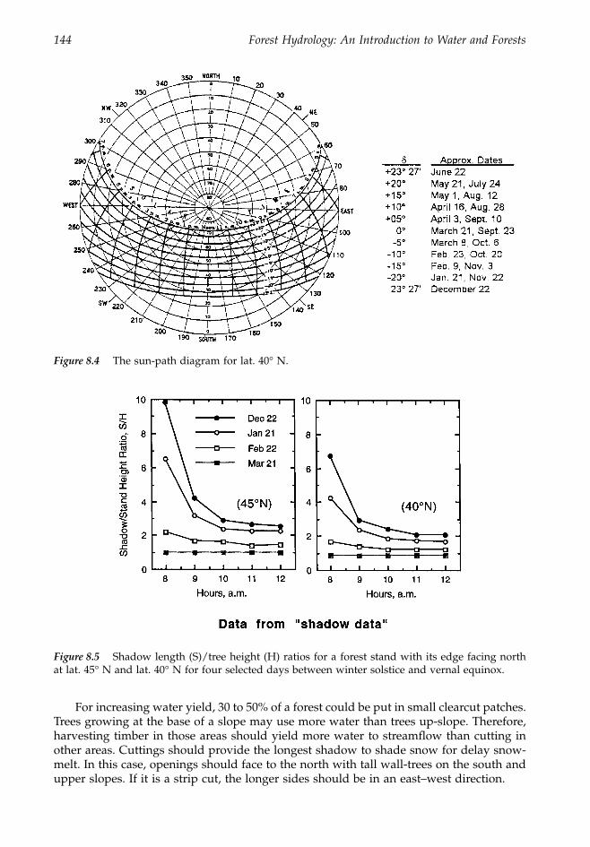
144 Forest Hydrology: An Introduction to Water and Forests
For increasing water yield, 30 to 50% of a forest could be put in small clearcut patches.Trees growing at the base of a slope may use more water than trees up-slope. Therefore,harvesting timber in those areas should yield more water to streamflow than cutting inother areas. Cuttings should provide the longest shadow to shade snow for delay snow-melt. In this case, openings should face to the north with tall wall-trees on the south andupper slopes. If it is a strip cut, the longer sides should be in an east–west direction.
Figure 8.4 The sun-path diagram for lat. 40∞ N.
Figure 8.5 Shadow length (S)/tree height (H) ratios for a forest stand with its edge facing northat lat. 45∞ N and lat. 40∞ N for four selected days between winter solstice and vernal equinox.
1363_C08_fm Page 144 Wednesday, December 4, 2002 7:42 AM
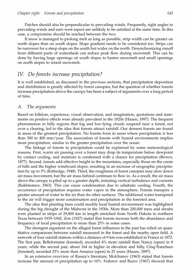
Chapter eight: Forests and precipitation 145
Patches should also be perpendicular to prevailing winds. Frequently, right angles toprevailing winds and east–west aspect are unlikely to be satisfied at the same time. In thiscase, a compromise should be reached between the two.
If snow is managed to prolong melt as long as possible, strip width can be greater onnorth slopes than on south slopes. Slope gradient needs to be considered too. Strips canbe narrower for a steep slope on the south but wider on the north. Desynchronizing runofffrom different parts of watersheds can reduce peak flow during snowmelt. This can bedone by having large openings on south slopes to hasten snowmelt and small openingson north slopes to retard snowmelt.
IV. Do forests increase precipitation?It is well established, as discussed in the previous sections, that precipitation depositionand distribution is greatly affected by forest canopies, but the question of whether forestsincrease precipitation above the canopy has been a subject of arguments over a long periodof time.
A. The arguments
Based on folklore, experience, visual observation, and imagination, quotations and state-ments on positive effects were already prevalent in the 1820s (Hazen, 1897). The frequentphenomenon in hilly regions that fog and low-lying clouds suspend near a forest, notover a clearing, led to the idea that forests attract rainfall. Our densest forests are foundin areas of the greatest precipitation. No forests form in areas where precipitation is lessthan 300 to 400 mm/year. The association of forests with humid environments impliesmore precipitation, similar to the greater precipitation over the ocean.
The linkage of forests to precipitation could be explained by some meteorologicalreasons. First, warm air passing over a forest may drop its temperature below dewpointby contact cooling, and moisture is condensed with a chance for precipitation (Brown,1877). Second, forests add effective height to the mountains, especially those on the crestsof hills and the higher windward slopes, resulting in an increase of orographic precipita-tion by up to 3% (Kittredge, 1948). Third, the roughness of forest canopies may slow downair-mass movement, but the air mass behind continues to flow in. As a result, the air massabove the canopy is piled up to a greater depth, initiating vertical turbulence and currents(Rakhmanov, 1963). This can cause condensation due to adiabatic cooling. Fourth, theoccurrence of precipitation requires water vapor in the atmosphere. Forests transpire agreater amount of water to the air than do other surfaces. The additional water transpiredto the air will trigger more condensation and precipitation in the forested area.
The idea that planting trees could modify local humid environment was highlightedduring the big drought of the Midwest in the 1930s. More than 200,000 trees and shrubswere planted in strips of 29,800 km in length stretched from North Dakota to northernTexas between 1935–1942. Zon (1927) stated that forests increase both the abundance andfrequency of local precipitation to more than 25% in some cases.
The strongest argument on the alleged forest influences in the past has relied on quan-titative comparisons between rainfall measured in the forest and the nearby open field. Anetwork of four rainfall stations within a distance of 9 km was established in France in 1872.The first pair, Bellefontaine (forested), recorded 4% more rainfall than Nancy (open) in 8years, while the second pair, about 164 m higher in elevation and hilly, Cinq-Tranchees(forested), recorded 25% more than Amance (open) in 25 years (Hazen, 1897).
In an extensive overview of Russia’s literature, Molchanov (1963) stated that forestsincrease the amount of precipitation up to 10%. Fedorov and Burov (1967) showed that
1363_C08_fm Page 145 Wednesday, December 4, 2002 7:42 AM
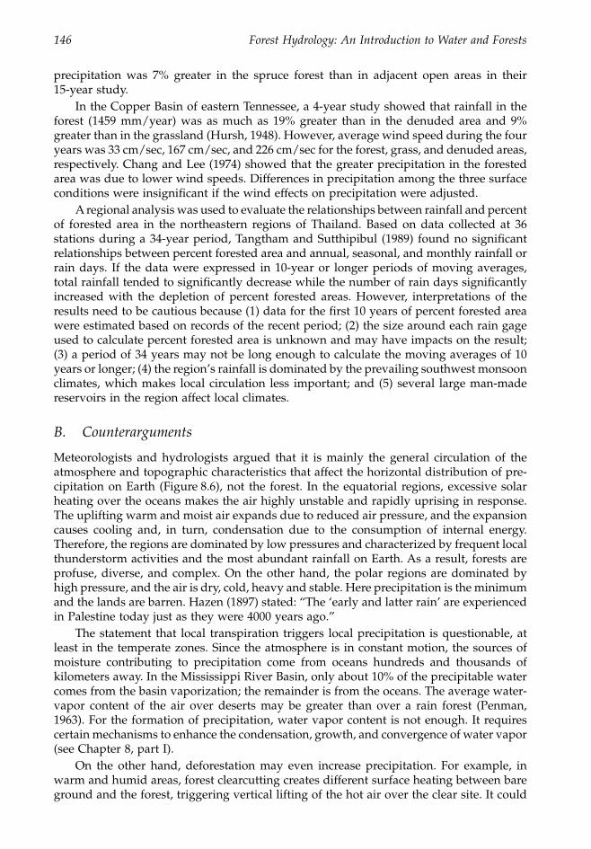
146 Forest Hydrology: An Introduction to Water and Forests
precipitation was 7% greater in the spruce forest than in adjacent open areas in their15-year study.
In the Copper Basin of eastern Tennessee, a 4-year study showed that rainfall in theforest (1459 mm/year) was as much as 19% greater than in the denuded area and 9%greater than in the grassland (Hursh, 1948). However, average wind speed during the fouryears was 33 cm/sec, 167 cm/sec, and 226 cm/sec for the forest, grass, and denuded areas,respectively. Chang and Lee (1974) showed that the greater precipitation in the forestedarea was due to lower wind speeds. Differences in precipitation among the three surfaceconditions were insignificant if the wind effects on precipitation were adjusted.
A regional analysis was used to evaluate the relationships between rainfall and percentof forested area in the northeastern regions of Thailand. Based on data collected at 36stations during a 34-year period, Tangtham and Sutthipibul (1989) found no significantrelationships between percent forested area and annual, seasonal, and monthly rainfall orrain days. If the data were expressed in 10-year or longer periods of moving averages,total rainfall tended to significantly decrease while the number of rain days significantlyincreased with the depletion of percent forested areas. However, interpretations of theresults need to be cautious because (1) data for the first 10 years of percent forested areawere estimated based on records of the recent period; (2) the size around each rain gageused to calculate percent forested area is unknown and may have impacts on the result;(3) a period of 34 years may not be long enough to calculate the moving averages of 10years or longer; (4) the region’s rainfall is dominated by the prevailing southwest monsoonclimates, which makes local circulation less important; and (5) several large man-madereservoirs in the region affect local climates.
B. Counterarguments
Meteorologists and hydrologists argued that it is mainly the general circulation of theatmosphere and topographic characteristics that affect the horizontal distribution of pre-cipitation on Earth (Figure 8.6), not the forest. In the equatorial regions, excessive solarheating over the oceans makes the air highly unstable and rapidly uprising in response.The uplifting warm and moist air expands due to reduced air pressure, and the expansioncauses cooling and, in turn, condensation due to the consumption of internal energy.Therefore, the regions are dominated by low pressures and characterized by frequent localthunderstorm activities and the most abundant rainfall on Earth. As a result, forests areprofuse, diverse, and complex. On the other hand, the polar regions are dominated byhigh pressure, and the air is dry, cold, heavy and stable. Here precipitation is the minimumand the lands are barren. Hazen (1897) stated: “The ‘early and latter rain’ are experiencedin Palestine today just as they were 4000 years ago.”
The statement that local transpiration triggers local precipitation is questionable, atleast in the temperate zones. Since the atmosphere is in constant motion, the sources ofmoisture contributing to precipitation come from oceans hundreds and thousands ofkilometers away. In the Mississippi River Basin, only about 10% of the precipitable watercomes from the basin vaporization; the remainder is from the oceans. The average water-vapor content of the air over deserts may be greater than over a rain forest (Penman,1963). For the formation of precipitation, water vapor content is not enough. It requirescertain mechanisms to enhance the condensation, growth, and convergence of water vapor(see Chapter 8, part I).
On the other hand, deforestation may even increase precipitation. For example, inwarm and humid areas, forest clearcutting creates different surface heating between bareground and the forest, triggering vertical lifting of the hot air over the clear site. It could
1363_C08_fm Page 146 Wednesday, December 4, 2002 7:42 AM
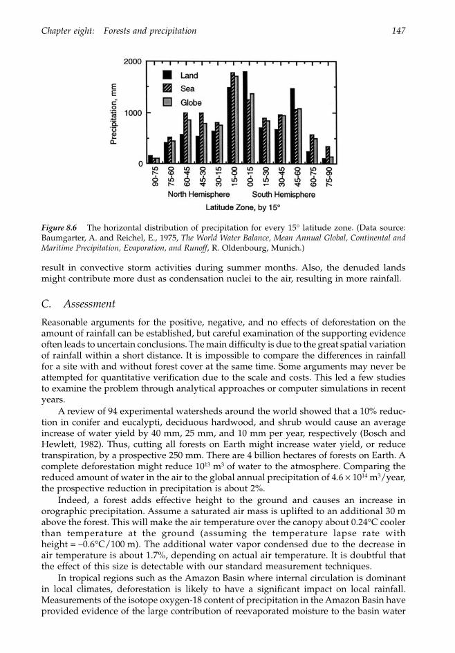
Chapter eight: Forests and precipitation 147
result in convective storm activities during summer months. Also, the denuded landsmight contribute more dust as condensation nuclei to the air, resulting in more rainfall.
C. Assessment
Reasonable arguments for the positive, negative, and no effects of deforestation on theamount of rainfall can be established, but careful examination of the supporting evidenceoften leads to uncertain conclusions. The main difficulty is due to the great spatial variationof rainfall within a short distance. It is impossible to compare the differences in rainfallfor a site with and without forest cover at the same time. Some arguments may never beattempted for quantitative verification due to the scale and costs. This led a few studiesto examine the problem through analytical approaches or computer simulations in recentyears.
A review of 94 experimental watersheds around the world showed that a 10% reduc-tion in conifer and eucalypti, deciduous hardwood, and shrub would cause an averageincrease of water yield by 40 mm, 25 mm, and 10 mm per year, respectively (Bosch andHewlett, 1982). Thus, cutting all forests on Earth might increase water yield, or reducetranspiration, by a prospective 250 mm. There are 4 billion hectares of forests on Earth. Acomplete deforestation might reduce 1013 m3 of water to the atmosphere. Comparing thereduced amount of water in the air to the global annual precipitation of 4.6 ¥ 1014 m3/year,the prospective reduction in precipitation is about 2%.
Indeed, a forest adds effective height to the ground and causes an increase inorographic precipitation. Assume a saturated air mass is uplifted to an additional 30 mabove the forest. This will make the air temperature over the canopy about 0.24∞C coolerthan temperature at the ground (assuming the temperature lapse rate withheight = –0.6∞C/100 m). The additional water vapor condensed due to the decrease inair temperature is about 1.7%, depending on actual air temperature. It is doubtful thatthe effect of this size is detectable with our standard measurement techniques.
In tropical regions such as the Amazon Basin where internal circulation is dominantin local climates, deforestation is likely to have a significant impact on local rainfall.Measurements of the isotope oxygen-18 content of precipitation in the Amazon Basin haveprovided evidence of the large contribution of reevaporated moisture to the basin water
Figure 8.6 The horizontal distribution of precipitation for every 15∞ latitude zone. (Data source:Baumgarter, A. and Reichel, E., 1975, The World Water Balance, Mean Annual Global, Continental andMaritime Precipitation, Evaporation, and Runoff, R. Oldenbourg, Munich.)
1363_C08_fm Page 147 Wednesday, December 4, 2002 7:42 AM
148 Forest Hydrology: An Introduction to Water and Forests
balance (Salati et al., 1979). A number of studies showed the actual percent of recycledwater varying between 35 and 50% (Salati et al., 1983). Using simulation models, thepotential impact of deforestation on rainfall in Amazon is a rainfall decrease of 600 to640 mm/year (Henderson-Sellers, 1981; Salati and Vose, 1983; Shukla et al., 1990).
It is therefore generally accepted by scientists that there is a significant impact ofdeforestation on rainfall in the tropical regions (Bruijnzeel, 1990), but the size of defores-tation and its levels of impacts require further study. Vertical circulation of transpiredwater in the temperate zones is probably insignificant. The amount of rainfall profits theforest, not the other way around.
ReferencesAlden, E.F., 1968, Moisture loss and weight of the forest floor under pole-size ponderosa pine stands,
J. For., 66, 70–71.Anderson, H.W. and Gleason, C.H., 1960. Logging and Brush Removal Effects on Runoff from Snow
Cover, IASH. Pub. No. 51, 478–489, Merelbeke, Belgium.Baumgarter, A. and Reichel, E., 1975, The World Water Balance, Mean Annual Global, Continental and
Maritime Precipitation, Evaporation, and Runoff, R. Oldenbourg, Munich.Bay, R.R., 1958, Cutting methods affect snow accumulation and melt in black spruce stands, Tech.
Notes 523, USDA Forest Service, Lake States Forest Exp. Sta.Berndt, H.W., 1965, Snow accumulation and disappearance in lodgepole pine clearcut blocks in Wy-
oming, J. For., 63, 88–91.Berris, S.N. and Harr, R.D., 1987, Comparative snow accumulation and melt during rainfall in forested
and clear cut plots in the western Cascades of Oregon, Water Resour. Res., 23, 135–142.Bosch, J.M. and Hewlett, J.D., 1982, A review of catchment experiments to determine the effect of
vegetation changes on water yield and evapotranspiration, J. Hydrology, 55, 3–23.Brown, J.C., 1877, Forest and Moisture, Simpkin, Marshall & Co., London.Bruijnzeel, L.A., 1990, Hydrology of Moist Tropical Forests and Effects of Conversion: A State of
Knowledge Review, UNESCO International Hydro. Programme.Burgy, R.H. and Pomeroy, C.R., 1958, Intercepted losses in grassy vegetation, Trans. Am. Geophy. Union,
39, 1095–1100.Caborn, J.M., 1964, Shelterbelts and Windbreaks, Faber & Faber, London.Chang, M., 1977, Is canopy interception an accurate measure of loss in the hydrologic budget? Texas
J. Sci., 18, 239–346.Chang, M. and Lee, R., 1974, Do Forests Increase Precipitation? West Virginia Forestry Notes, West
Virginia University, 2, 16–20.Changnon, S.A., Jr. and Jones, D.M.A., 1972, Review of the influences of the Great Lakes on weather,
Water Resour. Res., 8, 360–371.Ekern, P.C., 1964, Direct interception of cloud water on Lanaihale, Hawaii, Soil Sci. Soc. Am. Proc., 28,
419–421.Fedorov, S.F. and Burov, A.S., 1967, Influence of the forest on precipitation, in Soviet Hydrology: Selected
Papers, AGU, Washington, DC, Vol. 3, pp. 217–224.Folliott, P.F., Gotterfried, G.J., and Baker, M.B., Jr., 1989, Water yield from forest snowpack management:
research findings in Arizona and New Mexico, Water Resour. Res., 25, 1999–2007.Gary, H.L., 1974, Snow accumulation and snowmelt as influenced by a small clearing in a lodgepole
pine forest, Water Resour. Res., 10, 348–353.Gary, H.L., 1979, Duration of snow accumulation increases after harvesting in Lodgepole pine in
Wyoming and Colorado, Res. Note RM-266, U.S. Forest Service.Gary, H.L., 1980, Patch clearcut to manage snow in lodgepole pine, in Watershed Management 1980,
Proc. ASCE, pp. 335–348.Gary, H.L. and Troendle, C.A., 1982, Snow accumulation and melt under various stand densities in
Lodgepole pine in Wyoming and Colorado, Res. Note RM-417, USDA Forest Service, RockyMountain Forest and Range Esp. Sta.
Gash, J.H., 1979, An analytical model of rainfall interception by forests, Q. J. R. Meteoro. Soc., 105, 43–55.
1363_C08_fm Page 148 Wednesday, December 4, 2002 7:42 AM
Chapter eight: Forests and precipitation 149
Golding, D.L. and Swanson, D.H., 1978, Snow accumulation and melt in small forest openings inAlberta, Can. J. For. Res., 8, 380–388.
Goodell, B.C., 1952, Watershed management aspects of thinned young lodgepole pine stands, J For.,50, 374–378.
Goodman, J., 1985, The collection of fog drip, Water Resour. Res., 21, 392–394.Gower, S.T. and Son, Y., 1992, Differences in soil and leaf litterfall nitrogen dynamics for five forest
plantations, Soil Sci. Soc. Am. J., 56, 1959–1966.Gray, D.M. and Male, D.H., 1981, Handbook of Snow, Pergamon Press, Elmsford, N.Y.Harr, R.D., 1966, Influence of Intercepted Water on Evapotranspiration from Small Potted Trees. Ph.D.
dissertation, Colorado State University, Fort Collins.Harr, R.D., 1982, Fog drip in the Bull Run municipal watershed, Oregon, Water Resour. Bull,. 18, 785–788.Harris, A.S., 1989, Wind in the Forests of Southeast Alaska and Guides for Reducing Damage, Gen.
Tech. Rep. PNW-GTR-244, U.S. Forest Service.Haupt, H.F., 1979, Effects of Timber Cutting and Revegetation on Snow Accumulation and Melt in
North Idaho, Res. Paper INT-224, U.S. Forest Service.Hazen, H.A., 1897, Forests and rainfall, in Proc. Am. Forestry Congress, the 7th Annual Meeting, pp.
133–139.Helvey, J.D., 1967, Interception by eastern white pine, Water Resour. Res., 3, 723–729.Helvey, J.D., 1971, A summary of rainfall interception by certain conifers of North America, in Biological
Effects of the Hydrologic Cycle., Proc. 3rd Intl Seminar. Hydro. Prof., Lafayette, IN, pp. 103–113.Helvey, J.D. and Patric, J.J., 1965, Canopy and litter interception of rainfall by hardwoods of eastern
United States, Water Resour. Res., 1, 193–206.Henderson-Sellers, A., 1981, Climatic sensitivity to variations in vegetated land surface albedos, in
Proc., 6th Annual Climate Diagnostics Workshop, Columbia University, Oct. 14–16, 1981, pp.135–144.
Hoover, M.D. and Leaf, C.F., 1967, Process and significance of interception in Colorado subalpineforest, in Forest Hydrology, Sopper, W.E. and Lull, H.W., Eds., Pergamon Press, Elmsford, NY,pp. 213–224.
Hursh, C.R., 1948, Local Climate in the Copper Basin of Tennessee as Modified by the Removal ofVegetation, USDA Circular 774.
Kattelmann, R.C., 1982, Water yield improvement in the Sierra Nevada snow zone: 1912–1982, in Proc.50th Western Snow Conf., Reno, Nevada, pp. 39–48.
Kaufmann, M.R., Edminster, C.E., and Troendle, C.A., 1982, Leaf Area Determination for SubaplineTree Species in the Central Rocky Mountains, Res. Paper RM-238, USDA Forest Service.
Kittredge, J., 1948, Forest Influences, McGraw-Hill, New York.Kittredge, J., 1953, Influence of forests on snow in the ponderosa pine–sugar pine–fir zone in the
Central Sierra Nevada, Hilgardia, 21, 1–96.Lee, R., 1978, Forest Microclimatology, Columbia University Press, New York.List, R.J., 1971, Smithsonian Meteorological Tables, 6th rev. edition, Smithsonian Institution Press, Wash-
ington, D.C.Molchanov, A.A., 1963, The Hydrological Role of Forests, Israel Program for Sci. Translations, Jerusa-
lem, Office of Tech. Service, US Dept. Commerce, Washington, D.C.Monteith, J.L. and Unsworth, M.H., 1990, Principles of Environmental Physics, Edward Arnold, London.Naegeli, W., 1946, Further investigation on wind conditions in the range of shelterbelts, Mitteil. Schweiz.
Anstalt Forstl. Versuchsw., 24, 659–737.Niederhof, C.H. and Dunford, E.G., 1942, The effect of openings in a young lodgepole pine forest on
the storage and melting of snow, J. For., 40, 802–805.Penman, H.L., 1963, Vegetation and Hydrology, Commonwealth Agr. Bureaux, Tech. Communication
No. 53. Farnham Royal, Bucks, England.Rakhmanov, V.V., 1963, Dependence of the amount of precipitation on the wooded area in the plains
of the European USSR, Meteoro. Geoastrophysical Abs., 14, 712.Rosa, J.M., 1956, Forest snowmelt and spring floods, J. For., 84, 231–135.Roth, F.A., II and Chang, M., 1981, Throughfall in planted stands of four southern pine species in East
Texas, Water Resour. Bull., 17, 880–885.
1363_C08_fm Page 149 Wednesday, December 4, 2002 7:42 AM
150 Forest Hydrology: An Introduction to Water and Forests
Rusk, C.R., 1969, Interception of Precipitation by Forest Canopies and Litter, M.S. thesis, Universityof Tennessee, Knoxville.
Rutter, A.J. and Morton, A.J., 1977, A predictive model of rainfall interception in forests. III: Sensitivityof the model to stand parameters and meteorological variables, J. Appl. Ecol., 14, 567–588.
Rutter, A.J., Morton, A.J., and Robins, P.C. 1975, A predictive model of rainfall interception in forests.II: Generalization of the model and comparison with observations in some coniferous andhardwood stands, J. Appl. Ecol., 12, 367–380.
Salati, E. et al., 1979, Recycling of water in the Amazon Basin: an isotopic study, Water Resour. Res., 15,1250–1258.
Salati, E., Lovejoy, T.E., and Vose, P.B., 1983, Precipitation and water recycling in tropical rain forestswith special reference to the Amazon Basin, Environmentalist, 3, 67–72.
Salati, E. and Vose, P.B., 1983, Analysis of amazon hydrology in relation to geoclimatic factors andincreased deforestation, Beitrage zur Hydrologie, 9, 11–22.
Satterlund, D.R. and Adams, P.W., 1992, Wildland Watershed Management, 2nd ed., John Wiley & Sons,New York.
Shih, S.F., 1989, Relating calculated leaf area index, evapotranspiration, and irrigation method ofsugarcane, Agron. J., 81,111–115.
Shukla, J., Nobre, C., and Sellers, P.J., 1990, Amazon deforestation and climatic chang, Science, 247,1322–1325.
Singer, M.J. and Blackard, J., 1978, Effect of mulching on sediment in runoff from simulated rainfall,Soil Sci. Soc. Am. J., 42, 481–486.
Singh, B. and Szeics, G., 1979, The effect of intercepted rainfall on the water balance of a hardwoodforest, Water Resour. Res., 15, 131–138.
Small, R.T., 1966, Terrain effects on precipitation in Washington State, Weatherwise, October, 204–207.Stewart, J.B., 1977, Evaporation from the wet canopy of a pine forest, Water Resour. Res., 13, 915–921.Sturges, D.L., 1983, Shelterbelt Establishment and Growth at a Windswept Wyoming Rangeland Site,
Res. Paper RM-243, U.S. Forest Service.Swank, W.T., Goebel, N.B., and Helvey, J.D., 1972, Interception loss in loblolly pine stands of the South
Carolina piedmont, J. Soil Water Conserv., 27, 160–164.Swank, W.T. and Schreuder, H.T., 1974, Comparison of three methods of estimating surface and
biomass for a forest of young eastern white pine, Forest Sci., 20, 91–100.Tangtham, N. and Sutthipibul, V., 1989, Effects of diminishing forest area on rainfall amount and
distribution in North-East Thailand, in Regional Seminar on Tropical Forest Hydrology, Sept.4–9, Institute Penyelidikan Perhutanan Malaysia, Kuala Lumpur, Malaysia.
Thoroud, D.B., 1967, The effect of applied interception rates on potted ponderosa pine, Water Resour.Res., 3, 443–450.
Troendle, C.A. and Leaf, C.F., 1981, Effects of timber harvest in the snow zone on volume and timingof water yield, in Interior West Watershed Management, Baumgartner, D.M., Ed., WashingtonState University, Pullman, pp. 231–243.
Unger, P.W. and Parker, J.J., 1976, Evaporation reduction from soil with wheat, sorghum, and cottonresidues, Soil Sci. Soc. Am. J., 40, 938–942.
U.S. Water News, 1994, Chilean fog collection system furnishes daily baths, U.S. Water News, 11,: 2.WMO, 1964, Windbreaks and Shelterbelts, World Meteoro. Org., Tech. Note No. 59, WMO-No.
147.TP.70, Geneva, Switzerland. Zinke, P.J., 1967, Forest interception studies in the United States, in International Symposium on Forest
Hydrology, Sopper, W.E. and Lull, H.W., Eds.,. Pergamon Press, Elmsford, NY.Zon, R., 1927, Forests and Water in the Light of the Scientific Investigation, U.S. National Waterways
Comm., Final Rep. 1912 (Senate Document No. 469, 62nd Congress, 2nd Session).
1363_C08_fm Page 150 Wednesday, December 4, 2002 7:42 AM
151
chapter nine
Forests and vaporization
Contents
I. Vaporization processes ...................................................................................................152A. Water surface ...........................................................................................................152B. Bare soils ..................................................................................................................153C. Vegetative surfaces .................................................................................................154
II. Sources of energy ............................................................................................................155A. Net radiation............................................................................................................155B. Energy dissipation ..................................................................................................157
1. Sensible heat ......................................................................................................1572. Conductive heat ................................................................................................1573. Latent heat .........................................................................................................1614. Proportionality ..................................................................................................161
C. Extraterrestrial radiation........................................................................................162III. Evapotranspiration..........................................................................................................163
A. Potential evapotranspiration.................................................................................1631. Thornthwaite (1948) model.............................................................................1632. Hamon (1963) method .....................................................................................1643. Penman (1948) method ....................................................................................1644. Penman-Monteith method ..............................................................................166
B. Actual evapotranspiration.....................................................................................1661. The hydrologic balance approach..................................................................1672. Lysimeters ..........................................................................................................1673. Soil-moisture depletion approach..................................................................167
IV. Forested vs. nonforested ................................................................................................168A. Environmental conditions .....................................................................................168B. Forested watersheds...............................................................................................169C. Forest species...........................................................................................................169
References .....................................................................................................................................171
Vaporization refers to the change of water from liquid state into vapor state. It occurs onwater, snow, soil, and vegetation surfaces and is a negative item in the hydrologic balanceof a watershed system. The loss of water is commonly termed evaporation when it occurson water, snow, and soil surfaces, transpiration when it occurs on vegetation surfaces, andevapotranspiration as the total loss of water in vapor state. In addition, the process bywhich snow and ice dissipate due to melting and evaporation is referred to as ablation.
1363_C09_fm Page 151 Wednesday, December 4, 2002 7:43 AM
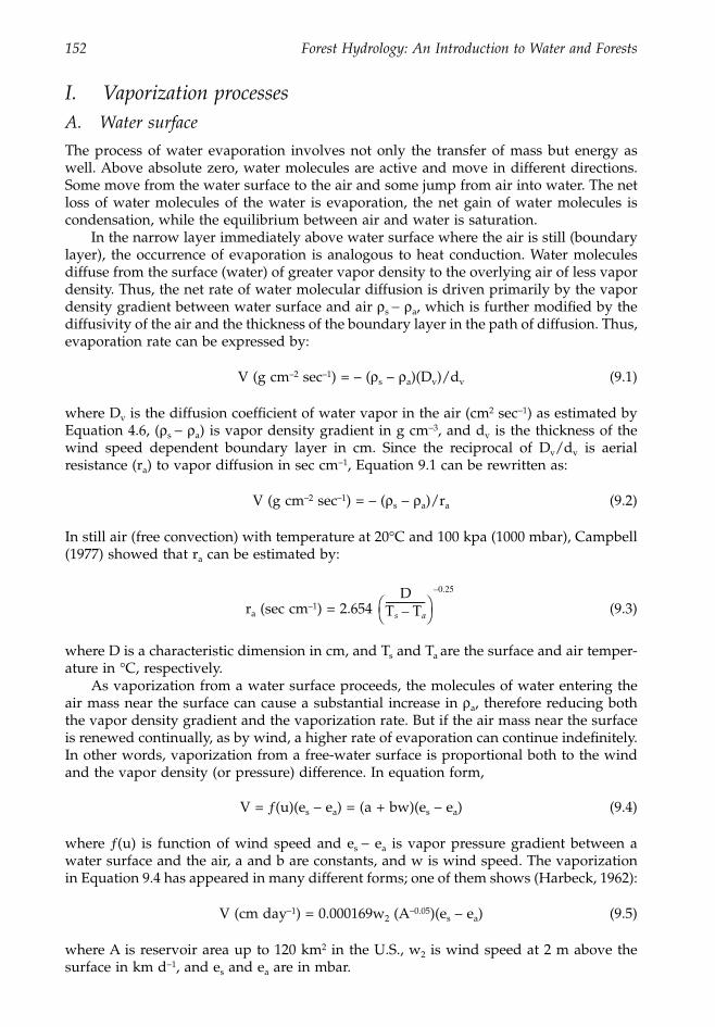
152 Forest Hydrology: An Introduction to Water and Forests
I. Vaporization processes
A. Water surface
The process of water evaporation involves not only the transfer of mass but energy aswell. Above absolute zero, water molecules are active and move in different directions.Some move from the water surface to the air and some jump from air into water. The netloss of water molecules of the water is evaporation, the net gain of water molecules iscondensation, while the equilibrium between air and water is saturation.
In the narrow layer immediately above water surface where the air is still (boundarylayer), the occurrence of evaporation is analogous to heat conduction. Water moleculesdiffuse from the surface (water) of greater vapor density to the overlying air of less vapordensity. Thus, the net rate of water molecular diffusion is driven primarily by the vapordensity gradient between water surface and air
r
s
-
r
a
, which is further modified by thediffusivity of the air and the thickness of the boundary layer in the path of diffusion. Thus,evaporation rate can be expressed by:
V (g cm
–2
sec
–1
) = – (
r
s
–
r
a
)(D
v
)/d
v
(9.1)
where D
v
is the diffusion coefficient of water vapor in the air (cm
2
sec
-
1
) as estimated byEquation 4.6, (
r
s
-
r
a
) is vapor density gradient in g cm
-
3
, and d
v
is the thickness of thewind speed dependent boundary layer in cm. Since the reciprocal of D
v
/d
v
is aerialresistance (r
a
) to vapor diffusion in sec cm
-
1
, Equation 9.1 can be rewritten as:
V (g cm
–2
sec
–1
) = – (
r
s
–
r
a
)/r
a
(9.2)
In still air (free convection) with temperature at 20
∞
C and 100 kpa (1000 mbar), Campbell(1977) showed that r
a
can be estimated by:
r
a
(sec cm
–1
) = 2.654 (9.3)
where D is a characteristic dimension in cm, and T
s
and T
a
are the surface and air temper-ature in
∞
C, respectively.As vaporization from a water surface proceeds, the molecules of water entering the
air mass near the surface can cause a substantial increase in
r
a
, therefore reducing boththe vapor density gradient and the vaporization rate. But if the air mass near the surfaceis renewed continually, as by wind, a higher rate of evaporation can continue indefinitely.In other words, vaporization from a free-water surface is proportional both to the windand the vapor density (or pressure) difference. In equation form,
V =
(u)(e
s
– e
a
) = (a + bw)(e
s
– e
a
) (9.4)
where
(u) is function of wind speed and e
s
-
e
a
is vapor pressure gradient between awater surface and the air, a and b are constants, and w is wind speed. The vaporizationin Equation 9.4 has appeared in many different forms; one of them shows (Harbeck, 1962):
V (cm day
–1
) = 0.000169w
2
(A
–0.05
)(e
s
– e
a
) (9.5)
where A is reservoir area up to 120 km
2
in the U.S., w
2
is wind speed at 2 m above thesurface in km d
-
1
, and e
s
and e
a
are in mbar.
DTs Ta–----------------
Ë ¯Ê �
0.25–
1363_C09_fm Page 152 Wednesday, December 4, 2002 7:43 AM
Chapter nine: Forests and vaporization 153
The saturated vapor pressure of water, e
s
, is very sensitive to changes in temperature.It increases by about 7% for every 1
∞
C increase in temperature between 10 and 30
∞
C.However, temperature has only a small effect on the vapor pressure of an air mass, e
a,
sothe difference, e
s
-
e
a
, is largely a temperature function.
B. Bare soils
Evaporation from a wet, bare soil surface is similar to that from a water surface and occursat the potential rate as determined by meteorological factors and by the energy availableto change the state of water (often referred to as Stage I). As evaporation proceeds, soilmoisture is reduced, the soil profile cannot supply water to sustain atmospheric evapo-rativity, and the evaporation rate falls steadily below the potential rate. During this fallingstage of drying (Stage II), the evaporation rate is primarily determined by the water-flowproperties within the soil, namely hydraulic conductivity. When the surface zone becomesso dry that liquid flux of water virtually ceases, water transmission occurs through vaporflux as governed by soil vapor diffusivity. Soil vapor diffusivities are affected by soilmoisture content, temperature, and pressure. The evaporation rate at this vapor-diffusionstage (Stage III) is slow and steady. It can persist for a long period of time until water issupplied to the soil again by precipitation or irrigation.
For a semiinfinite, initially saturated soil subjected to infinite evaporativity, the cumu-lative evaporation E (cm) and the evaporation flux e (cm/day
-
1
) during the first and secondstages of drying are related to square root of time (t, days) and the weighted meandiffusivity ( , cm
2
d
-
1
) by these equations (Gardner, 1959; Hillel, 1982):
E = 2(
q
i
-
q
f
)[ t/
p
]
0.5
(9.6)
e = (
q
i
-
q
f
)[ /(
p
t)]
0.5
(9.7)
where
q
i
and
q
f
are the initial profile wetness and final surface wetness in fractions ofvolume. For a soil with
q
I
= 0.45 (45%),
q
f
(air-dry) = 0.05 (5%), and = 100 cm
2
/d, thecumulative E at the end of 5 days = 2(0.45 – 0.05)[100
¥
5/3.1416]
0.5
= 10.09 cm, and themean e at the fifth day = 0.40[100/(3.1416
¥
5)]
0.5
= 1.01 cm day
-
1
.The vapor flux of a soil is affected by vapor diffusion coefficient and vapor pressure
gradient as described by the following equation (Hanks, 1958; Jalota and Prihar, 1998):
(9.8)
where
q = water vapor flow rate, g cm
-
2
sec
-
1
D = diffusivity of water vapor into still air, cm
2
sec
-
1
P = the atmospheric pressure, dyn cm
-
2
(1 atm = 1.013
¥
10
6
dyn cm
-
2
)P
v
= water vapor in the soil, dyn m
-
2
R = gas constant, 8.314
¥
10
7
dyn-cm
∞
K
-
1
mol
-
1
T = soil temperature,
∞
KM = molecular weight of water vapor (=18 g mol
-
1
)dP
v
/dX = vapor pressure gradient in a dry layer X, dynes cm
-
2
cm
a
= tortuosity factor (taken as 0.87 for silt loam and 0.66 for sandy loam)
f
= volume fraction of air-filled voids.
D
D
D
D
q = afDMRT---------- P
P – PV----------------
dPV
dX----------
1363_C09_fm Page 153 Wednesday, December 4, 2002 7:43 AM
154 Forest Hydrology: An Introduction to Water and Forests
The vapor flux is greater in soils with higher diffusivity, higher vapor pressure, and finertextures, but is lesser in soils with deeper drying layers. For a 3 cm layer of dry soil with
a
= 0.66,
f
= 0.58, D = 0.245 cm
2
sec
-
1
, T = 293
∞K, P = 1,023 ¥ 103 dyn cm-2, and Pv = 16 ¥ 103
dyn cm -2, the calculated q = 0.0037 ¥ 10-4 g cm-2/ sec-1, or 0.032 g cm-2 d–1 (0.032 cm day-1).Mulches have been used frequently as a management practice for reducing soil evap-
oration. However, they are effective only during the early stages of drying when climaticfactors dominate evaporation rate. During the drying stages, the soil surface begins to dryup and gradually forms a “self-mulch” that is more effective than gravel or other mulches(Hanks and Gardner, 1965). Also, tillage is generally thought to destroy soil structure andbreak down the capillaries. It causes the tilled layer to dry out quickly, retards liquidmovement of water from the underlying untilled layer, and keeps the lower portion ofthe tilled layer moist. Recent studies showed that the upward capillary flow was notcompletely cut off by tillage; it was only retarded because of the decrease in vapordiffusivity (Jalota and Prihar, 1998).
C. Vegetative surfaces
Water loss from vegetative surfaces, or transpiration, is basically an evaporation processexcept that its active surface is through stomata or cuticles on leaves and lenticels on bark,and water is conducted through the root system. Thus, compared to water loss per unitarea of soil, transpiration has a greater and deeper evaporating sphere. This means thatwhile the rate of soil evaporation is reduced because of the depletion of water contentnear the surface, transpiration can continue to be active because water deeper in the soilcan still be available through plant root systems.
Water potential is a term often used in plant physiology and soil physics to describethe status of water in terms of energy level. A potential is defined as the work requiredto move a unit mass of water from a reference point of pure free water (the potential y = 0)to the point in question (y = -works/mass or ergs/g; tension, suction or negative pres-sure). When water potential in the stomata is greater than the air, water in the stomata isvaporized to the air due to vapor pressure gradient, es - ea. The losses of water to the aircause the total water potential in the stomata to be less than that in adjacent cells. Thiscauses water in the adjacent cells to move to the stomata and thus form a driving forcefrom the stomata all the way to root tips and surrounding soils. In equation form, tran-spiration Tr can be expressed by:
Tr = –3600(cpra)/(gLv)[De/(rc + ra)] (9.9)
where cp is the specific heat of air (cal g-1 ∞C-1), ra is the air density (g cm-3), g is thepsychrometric constant (from 0.654 to 0.670 mbar ∞C-1, 0 to 30 ∞C, De is the saturation vaporpressure deficit of the air (mbar) or es - ea, the denominators rc and ra are canopy and aerialresistance (generally <10 sec cm-1) respectively, Lv is the latent heat of vaporization (cal/g-1,Equation 4.1), and constant 3600 converts the result Tr from cm sec-1 into cm h-1.
Equation 9.9 is basically a calculation of total energy used for transpiration and thenconverts the total (latent) energy into the depth of water per unit area. The terms(cpra)/(gLv) are relatively constant, making De/(rc + ra) the determining factors of transpi-ration rate. The De is very sensitive to canopy temperature and relative humidity of theair, while rc and ra are affected by wind speed and canopy height. Generally, rc is greaterthan ra (Lee, 1980), and ra decreases with the height of vegetation (Shuttleworth, 1993).Thus, a smaller value of aerial resistance means more efficient water vapor diffusion inthe air.
1363_C09_fm Page 154 Wednesday, December 4, 2002 7:43 AM
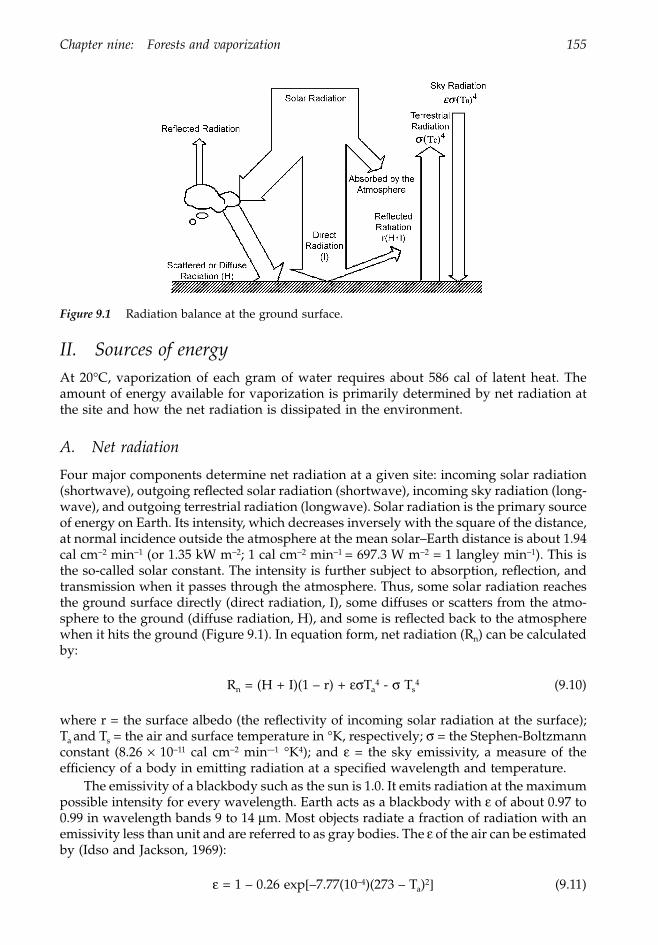
Chapter nine: Forests and vaporization 155
II. Sources of energyAt 20∞C, vaporization of each gram of water requires about 586 cal of latent heat. Theamount of energy available for vaporization is primarily determined by net radiation atthe site and how the net radiation is dissipated in the environment.
A. Net radiation
Four major components determine net radiation at a given site: incoming solar radiation(shortwave), outgoing reflected solar radiation (shortwave), incoming sky radiation (long-wave), and outgoing terrestrial radiation (longwave). Solar radiation is the primary sourceof energy on Earth. Its intensity, which decreases inversely with the square of the distance,at normal incidence outside the atmosphere at the mean solar–Earth distance is about 1.94cal cm-2 min-1 (or 1.35 kW m-2; 1 cal cm-2 min-1 = 697.3 W m-2 = 1 langley min-1). This isthe so-called solar constant. The intensity is further subject to absorption, reflection, andtransmission when it passes through the atmosphere. Thus, some solar radiation reachesthe ground surface directly (direct radiation, I), some diffuses or scatters from the atmo-sphere to the ground (diffuse radiation, H), and some is reflected back to the atmospherewhen it hits the ground (Figure 9.1). In equation form, net radiation (Rn) can be calculatedby:
Rn = (H + I)(1 – r) + esTa4 - s Ts
4 (9.10)
where r = the surface albedo (the reflectivity of incoming solar radiation at the surface);Ta and Ts = the air and surface temperature in ∞K, respectively; s = the Stephen-Boltzmannconstant (8.26 ¥ 10-11 cal cm-2 min--1 ∞K4); and e = the sky emissivity, a measure of theefficiency of a body in emitting radiation at a specified wavelength and temperature.
The emissivity of a blackbody such as the sun is 1.0. It emits radiation at the maximumpossible intensity for every wavelength. Earth acts as a blackbody with e of about 0.97 to0.99 in wavelength bands 9 to 14 mm. Most objects radiate a fraction of radiation with anemissivity less than unit and are referred to as gray bodies. The e of the air can be estimatedby (Idso and Jackson, 1969):
e = 1 – 0.26 exp[–7.77(10–4)(273 – Ta)2] (9.11)
Figure 9.1 Radiation balance at the ground surface.
1363_C09_fm Page 155 Wednesday, December 4, 2002 7:43 AM
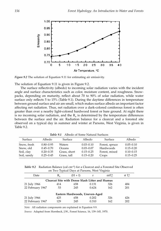
156 Forest Hydrology: An Introduction to Water and Forests
The solution of Equation 9.11 is given in Figure 9.2.The surface reflectivity (albedo) to incoming solar radiation varies with the incident
angle and surface characteristics such as color, moisture content, and roughness. Snow-packs, depending on maturity, reflect about 70 to 90% of solar radiation, while watersurface only reflects 5 to 15% (Table 9.1). During the daytime differences in temperaturebetween ground surface and air are small, which makes surface albedo an important factoraffecting net radiation. Thus, net radiation over a dark-colored coniferous forest is oftengreater than over a nearby light-colored hardwood forest or bare ground. At night thereis no incoming solar radiation, and the Rn is determined by the temperature differencesbetween the surface and the air. Radiation balance for a clearcut and a forested siteobserved on a typical day in summer and winter at Parsons, West Virginia, is given inTable 9.2.
Figure 9.2 The solution of Equation 9.11 for estimating air emissivity.
Table 9.1 Albedo of Some Natural Surfaces
Surface Albedo Surface Albedo Surface Albedo
Snow, fresh 0.80–0.95 Waters 0.03–0.10 Forest, spruce 0.05–0.10Snow, old 0.45–0.70 Oceans 0.03–0.07 Hardwoods 0.15–0.20Soil, clay 0.20–0.35 Grass, short 0.15–0.25 Forest, mixed 0.10–0.15Soil, sandy 0.25–0.45 Grass, tall 0.15–0.20 Crops 0.15–0.25
Table 9.2 Radiation Balance (cal cm----2) for a Clearcut and a Forested Site Observed on Two Typical Days at Parsons, West Virginia
Date Rn (H + I) r esTa4 s Ts
4
Clearcut Site with Dense Slash Litter and Humus21 July 1966 414 658 0.131 326 48422 February 1967 53 245 0.624 162 201
Eastern Hardwoods, Uneven-Aged21 July 1966 425 658 0.202 326 42622 February 1967 129 245 0.310 162 202
Note: All radiation components are explained in Equation 9.9.
Source: Adapted from Hornbeck, J.W., Forest Science, 16, 139–145, 1970.
1363_C09_fm Page 156 Wednesday, December 4, 2002 7:43 AM
Chapter nine: Forests and vaporization 157
B. Energy dissipation
The net radiation determined by Equation 9.9 for a given site is further dissipated intothree major components, sensible heat (Sh), latent heat (Lh), and conductive heat (Ch), or:
Rn = Sh + Lh + Ch (9.12)
The solution of Equation 9.10 requires measurements of incoming solar radiation H + I(also called global radiation). If the measurements are not available, Rn (cal cm-2 d-1) canbe estimated by:
Rn = Ra (1 – r)(0.3 + 0.5 n/N) – sTa[0.56 – 0.09(ed)0.5](0.1 + 0.9 n/N)(1440) (9.13)
where Ra = the daily solar radiation at the top of the atmosphere in cal cm-2 d-1 (Table 9.3or see Section C, “Extraterrestrial Radiation”), n/N = % of sunshine (Figure 9.3; Table 9.4);ed = the actual vapor pressure of the atmosphere in mm Hg; and r, s, and Ta are definedin Equation 9.10. Equation 9.13 is more reliable for long-term averages.
1. Sensible heatThe flow of heat between surface and air by convection is often referred to as sensibleheat flux. This is the heat transfer process with mass motions and affects air temperature.One of the methods to estimate sensible heat flux is to use the aerial resistance approach.Consider the equation:
Sh = – (cpra)(Ts – Ta)/(ra) (9.14)
where cp and ra have been defined previously, Ts and Ta are the surface and air temperaturerespectively in ∞C, and ra is the aerial resistance to the flow of sensible heat Sh. In the caseof forced (turbulent) convection for air at 20∞C and 1000 mbar (100 kpa), Campbell (1977)showed:
ra = 3.07 (D/W)0.5 (9.15)
and for free convection (at 20∞C and 1000 mbar), he gave:
ra = 2.656 (D/DT)0.25 (9.16)
where ra is in sec/cm, D is a characteristic dimension (the mean width for a leaf) in cm,W is the wind speed in cm/sec, and DT = Ts - Ta in ∞C. The negative sign in Equation9.14 means that heat fluxes from the surface toward the air. The S is positive if heat fluxesfrom the air toward the surface.
2. Conductive heatThe fraction of net radiation that is dissipated into the soil is heat conduction. The transferprocess occurs by the contact of soil particles; it does not change the shape of particles anddoes not require mass motions. Heat conduction into the soil profile is determined by thetemperature gradient and the thermal conductivity. Soil porosity, moisture content, andorganic-matter content make thermal conductivity different among soils. A typical dry soilcan have thermal conductivity of 4 to 8 ¥ 10-4 cal sec-1 cm-1 ∞C-1, while a wet soil can be of3 to 8 ¥ 10-3 cal sec-1 cm-1 ∞C-1, about ten times greater. In comparison, the thermal
1363_C09_fm Page 157 Wednesday, December 4, 2002 7:43 AM
158 Forest Hydrology: An Introduction to Water and Forests
Tabl
e 9.
3To
tal D
aily
Sol
ar R
adia
tion
by
Lat
itud
e Z
ones
at
Top
of t
he A
tmos
pher
e fo
r Se
lect
ed D
ays
Lat
itud
e(°
)M
arch
21
Apr
il
13M
ay
6Ju
ne
22Ju
ly
15A
ugus
t 8
Sept
embe
r 23
Oct
ober
16
Nov
embe
r 8
Dec
embe
r 22
Janu
ary
13Fe
brua
ry
4
N90
423
772
1077
949
765
8015
542
376
010
6098
075
415
37
7030
752
574
910
1293
474
230
312
924
2460
447
635
809
979
929
801
442
273
146
4973
146
5057
573
286
798
995
485
956
841
428
617
620
528
940
686
807
910
991
967
901
677
545
429
317
350
434
3077
586
592
997
596
092
176
566
356
446
649
456
820
841
894
923
935
930
916
831
760
685
605
630
691
1088
289
789
387
387
788
687
183
578
973
375
279
50
895
873
837
790
800
830
885
886
870
843
855
878
S10
882
824
760
687
704
753
871
910
927
933
936
936
2084
175
066
056
759
065
483
190
795
999
999
396
830
775
654
543
436
463
538
765
877
964
1041
1025
973
4068
653
841
329
732
840
967
781
994
410
5910
3295
350
575
408
276
165
192
274
568
743
901
1056
1018
909
6044
726
914
047
6813
944
264
484
010
4699
284
770
307
127
2323
303
532
778
1081
998
785
8015
57
153
429
790
1132
1046
796
9042
980
111
4910
6280
9
Not
e:
Bas
ed o
n th
e so
lar
cons
tant
1.9
4 ca
l/cm
-2 m
in–1
.
Sour
ce:
Lis
t, R
., 19
71, S
mit
hson
ian
Met
eoro
logi
cal T
able
s, 6
th r
evis
ed e
d.,
Smit
hson
ian
Inst
itut
ion
Pres
s, W
ashi
ngto
n, D
C..
1363_C09_fm Page 158 Wednesday, December 4, 2002 7:43 AM
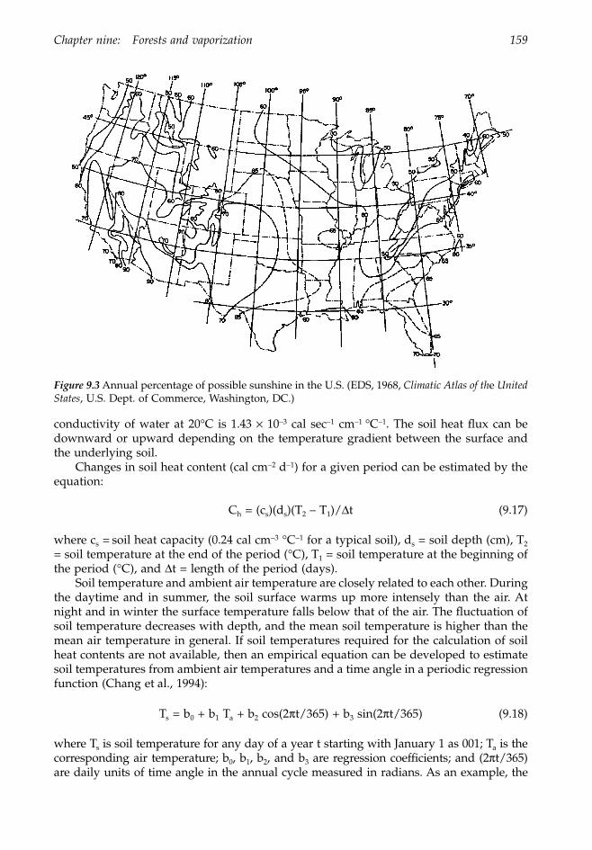
Chapter nine: Forests and vaporization 159
conductivity of water at 20∞C is 1.43 ¥ 10-3 cal sec-1 cm-1 ∞C-1. The soil heat flux can bedownward or upward depending on the temperature gradient between the surface andthe underlying soil.
Changes in soil heat content (cal cm-2 d-1) for a given period can be estimated by theequation:
Ch = (cs)(ds)(T2 – T1)/Dt (9.17)
where cs = soil heat capacity (0.24 cal cm-3 ∞C-1 for a typical soil), ds = soil depth (cm), T2
= soil temperature at the end of the period (∞C), T1 = soil temperature at the beginning ofthe period (∞C), and Dt = length of the period (days).
Soil temperature and ambient air temperature are closely related to each other. Duringthe daytime and in summer, the soil surface warms up more intensely than the air. Atnight and in winter the surface temperature falls below that of the air. The fluctuation ofsoil temperature decreases with depth, and the mean soil temperature is higher than themean air temperature in general. If soil temperatures required for the calculation of soilheat contents are not available, then an empirical equation can be developed to estimatesoil temperatures from ambient air temperatures and a time angle in a periodic regressionfunction (Chang et al., 1994):
Ts = b0 + b1 Ta + b2 cos(2pt/365) + b3 sin(2pt/365) (9.18)
where Ts is soil temperature for any day of a year t starting with January 1 as 001; Ta is thecorresponding air temperature; b0, b1, b2, and b3 are regression coefficients; and (2pt/365)are daily units of time angle in the annual cycle measured in radians. As an example, the
Figure 9.3 Annual percentage of possible sunshine in the U.S. (EDS, 1968, Climatic Atlas of the UnitedStates, U.S. Dept. of Commerce, Washington, DC.)
1363_C09_fm Page 159 Wednesday, December 4, 2002 7:43 AM
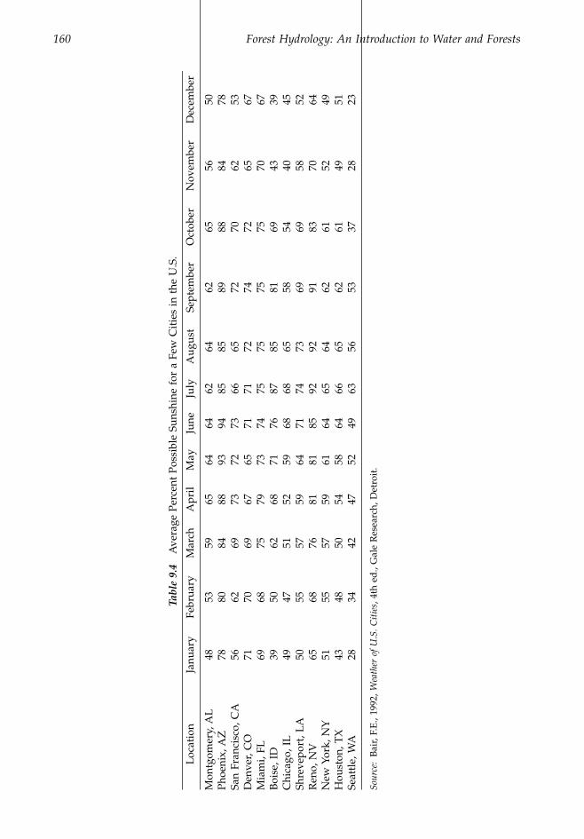
160 Forest Hydrology: An Introduction to Water and Forests
Tabl
e 9.
4A
vera
ge P
erce
nt P
ossi
ble
Suns
hine
for
a F
ew C
itie
s in
the
U.S
.
Loc
atio
nJa
nuar
yFe
brua
ryM
arch
Apr
ilM
ayJu
neJu
lyA
ugus
tSe
ptem
ber
Oct
ober
Nov
embe
rD
ecem
ber
Mon
tgom
ery,
AL
4853
5965
6464
6264
6265
5650
Phoe
nix,
AZ
7880
8488
9394
8585
8988
8478
San
Fran
cisc
o, C
A56
6269
7372
7366
6572
7062
53D
enve
r, C
O71
7069
6765
7171
7274
7265
67M
iam
i, FL
6968
7579
7374
7575
7575
7067
Boi
se, I
D39
5062
6871
7687
8581
6943
39C
hica
go, I
L49
4751
5259
6868
6558
5440
45Sh
reve
port
, LA
5055
5759
6471
7473
6969
5852
Ren
o, N
V65
6876
8181
8592
9291
8370
64N
ew Y
ork,
NY
5155
5759
6164
6564
6261
5249
Hou
ston
, TX
4348
5054
5864
6665
6261
4951
Seat
tle,
WA
2834
4247
5249
6356
5337
2823
Sour
ce:
Bai
r, F.
E.,
1992
, Wea
ther
of U
.S. C
itie
s, 4
th e
d.,
Gal
e R
esea
rch,
Det
roit
.
1363_C09_fm Page 160 Wednesday, December 4, 2002 7:43 AM
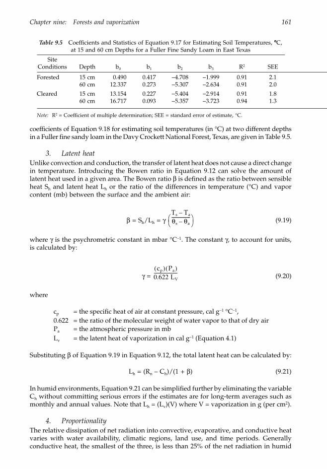
Chapter nine: Forests and vaporization 161
coefficients of Equation 9.18 for estimating soil temperatures (in ∞C) at two different depthsin a Fuller fine sandy loam in the Davy Crockett National Forest, Texas, are given in Table 9.5.
3. Latent heatUnlike convection and conduction, the transfer of latent heat does not cause a direct changein temperature. Introducing the Bowen ratio in Equation 9.12 can solve the amount oflatent heat used in a given area. The Bowen ratio b is defined as the ratio between sensibleheat Sh and latent heat Lh or the ratio of the differences in temperature (∞C) and vaporcontent (mb) between the surface and the ambient air:
b = Sh/Lh = g (9.19)
where g is the psychrometric constant in mbar ∞C-1. The constant g, to account for units,is calculated by:
g = (9.20)
where
cp = the specific heat of air at constant pressure, cal g-1 ∞C-1,0.622 = the ratio of the molecular weight of water vapor to that of dry airPa = the atmospheric pressure in mb Lv = the latent heat of vaporization in cal g-1 (Equation 4.1)
Substituting b of Equation 9.19 in Equation 9.12, the total latent heat can be calculated by:
Lh = (Rn – Ch)/(1 + b) (9.21)
In humid environments, Equation 9.21 can be simplified further by eliminating the variableCh without committing serious errors if the estimates are for long-term averages such asmonthly and annual values. Note that Lh = (Lv)(V) where V = vaporization in g (per cm2).
4. ProportionalityThe relative dissipation of net radiation into convective, evaporative, and conductive heatvaries with water availability, climatic regions, land use, and time periods. Generallyconductive heat, the smallest of the three, is less than 25% of the net radiation in humid
Table 9.5 Coefficients and Statistics of Equation 9.17 for Estimating Soil Temperatures, ∞∞∞∞C, at 15 and 60 cm Depths for a Fuller Fine Sandy Loam in East Texas
Site Conditions Depth b0 b1 b2 b3 R2 SEE
Forested 15 cm 0.490 0.417 -4.708 -1.999 0.91 2.160 cm 12.337 0.273 -5.307 -2.634 0.91 2.0
Cleared 15 cm 13.154 0.227 -5.404 -2.914 0.91 1.860 cm 16.717 0.093 -5.357 -3.723 0.94 1.3
Note: R2 = Coefficient of multiple determination; SEE = standard error of estimate, ∞C.
Ts Ta–qs qa–-----------------
Ë ¯Ê �
cp( ) Pa( )0.622 LV---------------------
1363_C09_fm Page 161 Wednesday, December 4, 2002 7:43 AM
162 Forest Hydrology: An Introduction to Water and Forests
areas and is negligible on an annual basis. A comparison of heat dissipation on threesurface conditions in Germany showed that net radiation was greatest over the forest,followed by grass and bare ground (Baumgartner, 1967). Only 5, 17, and 25% of the netradiation was dissipated into heat conduction for the forest, grass, and bare ground,respectively.
In humid environments, a great deal of energy is used for vaporization, causing latentheat to be greater than sensible heat. The situation is reversed in arid or semiarid areas.There the limited vaporization due to the lack of available water causes the conservedlatent heat to be used for warming the air. As a result, sensible heat is greater than latentheat. Thus, the Bowen ratio (sensible heat/latent heat) is usually less than 1.0 in humidregions and greater than 1.0 in semiarid regions. In the desert, the ratio can go above 3.0.
At higher latitudes, such as Copenhagen, Denmark, net radiation is negative duringwinter months and the energy for Lh comes largely from air masses of the warmer ocean.Thus, Lh exceeds Rn in the winter months, and Sh can take up more than 50% of Rn in thesummer. At Tempe, Arizona, strong advective energy from the nearby desert areas causesLh from a fully covered alfalfa field to exceed Rn every month of the year except Januaryand December (Pruitt, 1972).
C. Extraterrestrial radiation
As mentioned previously, virtually all energy utilized and exchanged in the biospherecomes from the sun. The radiant energy moves out from the sun in all directions andspreads over the surface of a sphere. At some distance r from the source Ro, the energyper unit area Rs is:
Rs = Ro/(4pr2) (9.22)
This means that the energy intercepted by surfaces of a given area declines with the squareof the distance from its source.
Solar radiation reduces to 1.94 cal cm–2 min-1 at the top of the atmosphere. This is theaverage flux at a surface perpendicular to the incoming solar radiation at the meansun–Earth distance. The daily extraterrestrial radiation Ra in cal cm-2 day-1 for a givengeographical location and time of the year can be estimated by (Shuttleworth, 1993):
Ra = 920dr (ws sinf sind + cosf cosd sinws) (9.23)
ws = cos–1 (–tanf tand) (9.24)
d = 0.4093 sin(2pJ/365 – 1.405) (9.25)
dr = 1 + 0.033cos (J) (9.26)
where
ws = the sunset hour angle in radiansdr = the relative distance between the Earth and the sund = the angle of solar declination in radiansJ = the Julian day number (April 15, J = 105)f = the site latitude in degrees (positive in the Northern Hemisphere and
negative in the Southern Hemisphere)
1363_C09_fm Page 162 Wednesday, December 4, 2002 7:43 AM
Chapter nine: Forests and vaporization 163
At f = 30oN and on April 15 (J = 105), the calculated d = 0.16 rad (9.186∞), ws = 1.664rad (95.357∞), dr = 0.9915, and Ra = 898 cal cm-2 day-1. The extraterrestrial radiationundergoes a great deal of change with respect to quantity, quality, and direction when itpasses through the atmosphere.
III. EvapotranspirationSeparating vaporization by different surfaces is not necessary in many practical applica-tions. A collective term, evapotranspiration (ET), often is used to describe the total vapor-ization for a given watershed. Evapotranspiration can be measured only under controlconditions; indirect observations or empirical and theoretical models are frequentlyemployed to make the estimates.
A. Potential evapotranspiration
The estimate of watershed ET losses is often referred to as the concept of potentialevapotranspiration (PE). It is, as defined by Thornthwaite (1948) and Penman (1963), thetotal water loss in vapor state from the center of an extended surface completely coveredby short, even-height green vegetation with no limit on water supply. This definitionemphasizes that (1) the advective heat exchanges to and from the surroundings are insig-nificant, (2) the heat flux from canopy to soil is negligible, (3) water loss is independentof vegetation and soil type, and (4) the solely limiting factor of PE is available energy.Thus, PE is the upper limit of ET under a given climatic condition and cannot exceed freewater evaporation. In practice, PE = ET if water supply to plants is unlimited or if monthlyPE is less than monthly precipitation.
The concept of PE is widely accepted and frequently applied in geographic studies,climate classifications, and water-resources research, planning, and management. How-ever, the PE concept is questionable if it is applied to small, forested watersheds. This isbecause of the tremendous effects on energy availability of forest density, species compo-sition, the physiological and phenological behavior of woody plants, topography, andadvective heat exchange. It also is invalid if it is applied to a body of pure water. Forexample, evaporation from a shallow pond exhibits a bell-shaped seasonal trend similarto air-temperature patterns. But, evaporation from a large, deep lake under similar weatherconditions can show an inverted bell-shaped pattern due to warmer water temperaturesin the cold season (Chang et al., 1976). These limitations imply that PE models should notbe applied in a short period of time and not be applied to an isolated field or a small,forested watershed.
1. Thornthwaite (1948) modelThis is one of the most widely used empirical models for estimating PE. It expressesPE as a function of air temperature (Tm) and a temperature dependent heat index (I).The estimated values (mm month-1), requiring adjustments in the length of the day fora 12-h period, are given by the following equation:
PE = 16(10Tm/I)a (K) (9.27)
where
I = the summation of monthly heat index i = Si = S (Tm/5)1.514
Tm = the monthly air temperature with m ranging from January to December
1363_C09_fm Page 163 Wednesday, December 4, 2002 7:43 AM
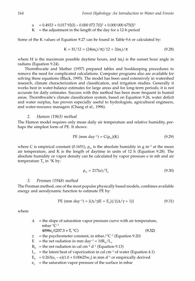
164 Forest Hydrology: An Introduction to Water and Forests
a = 0.4923 + 0.017 92(I) – 0.000 072 7(I)2 + 0.000 000 675(I)3
K = the adjustment in the length of the day for a 12-h period
Some of the K values of Equation 9.27 can be found in Table 9.6 or calculated by:
K = H/12 = [24(ws)/p]/12 = 2(ws)/p (9.28)
where H is the maximum possible daytime hours, and (ws) is the sunset hour angle inradians (Equation 9.24).
Thornthwaite and Mather (1957) prepared tables and bookkeeping procedures toremove the need for complicated calculations. Computer programs also are available forsolving these equations (Black, 1995). The model has been used extensively in watershedresearch, climate characterization and classification, and irrigation studies. Generally itworks best in water-balance estimates for large areas and for long-term periods; it is notaccurate for daily estimates. Success with this method has been more frequent in humidareas. Thornthwaite’s climate classification system, based on Equation 9.26, water deficitand water surplus, has proven especially useful to hydrologists, agricultural engineers,and water-resource managers (Chang et al., 1996).
2. Hamon (1963) methodThe Hamon model requires only mean daily air temperature and relative humidity, per-haps the simplest form of PE. It shows:
PE (mm day–1) = C(rw)(K) (9.29)
where C is empirical constant (0.1651), rw is the absolute humidity in g m-3 at the meanair temperature, and K is the length of daytime in units of 12 h (Equation 9.28). Theabsolute humidity or vapor density can be calculated by vapor pressure e in mb and airtemperature Ta in ∞K by:
rw = 217(e)/Ta (9.30)
3. Penman (1948) methodThe Penman method, one of the most popular physically based models, combines availableenergy and aerodynamic function to estimate PE by:
PE (mm day–1) = [(D/g)E + Eo)]/[(D/g + 1)] (9.31)
where
D = the slope of saturation vapor pressure curve with air temperature, mbar ∞C–1
4098es/(237.3 + T, °C) (9.32)g = the psychrometer constant, in mbar/∞C–1 (Equation 9.20)E = the net radiation in mm day-1 = 10Rn/Lv Rn = the net radiation in cal cm-2 d-1 (Equation 9.13)Lv = the latent heat of vaporization in cal cm-3 of water (Equation 4.1)Eo = 0.263(es - e)(1.0 + 0.00625w2) in mm d-1 or empirically derivedes = the saturation vapor pressure of the surface in mbar
1363_C09_fm Page 164 Wednesday, December 4, 2002 7:43 AM
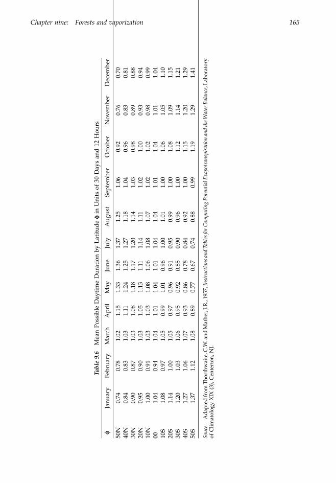
Chapter nine: Forests and vaporization 165
Tabl
e 9.
6M
ean
Poss
ible
Day
tim
e D
urat
ion
by L
atit
ude
ffff in
Uni
ts o
f 30
Day
s an
d 1
2 H
ours
fJa
nuar
yFe
brua
ryM
arch
Apr
ilM
ayJu
neJu
lyA
ugus
tSe
ptem
ber
Oct
ober
Nov
embe
rD
ecem
ber
50N
0.74
0.78
1.02
1.15
1.33
1.36
1.37
1.25
1.06
0.92
0.76
0.70
40N
0.84
0.83
1.03
1.11
1.24
1.25
1.27
1.18
1.04
0.96
0.83
0.81
30N
0.90
0.87
1.03
1.08
1.18
1.17
1.20
1.14
1.03
0.98
0.89
0.88
20N
0.95
0.90
1.03
1.05
1.13
1.11
1.14
1.11
1.02
1.00
0.93
0.94
10N
1.00
0.91
1.03
1.03
1.08
1.06
1.08
1.07
1.02
1.02
0.98
0.99
001.
040.
941.
041.
011.
041.
011.
041.
041.
011.
041.
011.
0410
S1.
080.
971.
050.
991.
010.
961.
001.
011.
001.
061.
051.
1020
S1.
141.
001.
050.
970.
960.
910.
950.
991.
001.
081.
091.
1530
S1.
201.
031.
060.
950.
920.
850.
900.
961.
001.
121.
141.
2140
S1.
271.
061.
070.
930.
860.
780.
840.
921.
001.
151.
201.
2950
S1.
371.
121.
080.
890.
770.
670.
740.
880.
991.
191.
291.
41
Souc
e:
Ad
apte
d fr
om T
hort
hwai
te, C
.W. a
nd M
athe
r, J.R
., 19
57, I
nstr
ucti
ons a
nd T
able
s for
Com
puti
ng P
oten
tial
Eva
potr
ansp
irat
ion
and
the W
ater
Bal
ance
, Lab
orat
ory
of C
limat
olog
y X
IX (
3), C
ente
rton
, NJ.
1363_C09_fm Page 165 Wednesday, December 4, 2002 7:43 AM
166 Forest Hydrology: An Introduction to Water and Forests
e = the actual vapor pressure of the air in mbarw2 = the wind speed at 2 m above the ground in km d–1
= wo(2/zo)0.15 (McCuen, 1998),(9.33)wo = the wind speed at the height of anemometer, km d–1
zo = the height of the anemometer, m
4. Penman-Monteith methodEquation 9.31 was originally developed for estimating open water evaporation and hasbeen modified to estimate PE and ET for various surface conditions and in differentregions. One of the modifications, made by Monteith (1965) and later discussed by Mon-teith (1985) and Monteith and Unsworth (1990), is to incorporate biologically based canopyand physically aerodynamic resistance parameters into the Penman’s wind function forestimating water-vapor diffusion over vegetated surfaces. The Penman-Monteith model,probably the most popular one, is of the following form:
ET = (9.34)
Where
D = the saturation vapor gradient, mbar ∞C-1 (Equation 9.32) g = the psychrometric constant, mbar ∞C-1 (Equation 9.20)Lv = the latent heat of vaporization, cal g-1 (Equation 4.1)cp = the specific heat of moist air (= 0.24 cal g-1 ∞C-1)ra = the density of air, g cm-3
Rn = the net radiation, cal cm-2 d-1
es = the saturation vapor pressure at surface, mbare = the actual vapor pressure of the air, mbarra = the aerodynamic resistance, sec cm-1
rs = the surface resistance, sec cm-1
Equation 9.34 can be used to estimate PE by setting rs = 0. However, both the Penmanand Penman-Monteith models require climatic data that are not usually available, partic-ularly the wind speed and resistance parameters. This limits their applicability.
B. Actual evapotranspiration
When water supply for vaporization is deficient or soil moisture content is below the fieldcapacity, then vaporization cannot proceed at the potential level. Thus, the actual evapo-transpiration (AE) is only a fraction of PE, or:
AE = a(PE) (9.35)
where the fraction a is affected not only by soil moisture content but also by climate andspecies. It is the so-called crop coefficient in agricultural irrigation. In the Lower CoastalPlain of Florida, direct measurements of 1-m tall slash pines growing on lysimeters showedthat the average AE was nearly identical to PE for the growing season (April to September)but only 75% for the dormant season (Riekerk, 1985).
1LV------
DRn Cpra es e–( )/ra+
D g 1 rs+( )/ra+--------------------------------------------------------
1363_C09_fm Page 166 Wednesday, December 4, 2002 7:43 AM
Chapter nine: Forests and vaporization 167
1. The hydrologic balance approachWatershed AE is often estimated indirectly by measuring the differences between water-shed precipitation (P) and runoff (RO). This is because P can be reliably estimated throughproper sampling, and RO is the only component in the hydrologic cycle that can be directlymeasured with great accuracy. Apparently, the estimate is valid only for a time intervallong enough to assure that those changes in soil moisture storage are negligible. If theestimate is for a period, such as month or season, with significant variation of moisturecontent, then changes in soil moisture storage need to be considered in the budget equationsolution.
In regions where the boundaries of surface watershed and underground watershedare not coincident, the measured RO is not reliable because of underground water leakage.The problem is more serious in small watersheds and becomes less significant as the sizeof watershed increases. It is important that the groundwater leakage be detected or thesite abandoned for hydrologic studies.
2. LysimetersA device that measures the quantity and quality of percolated water, or monitors the waterbudget, from an isolated block of soil in the field is called a lysimeter. Basically, it is a soiltank with growing plants inserted into the ground to simulate natural conditions. Rainor irrigation water percolated through the soil profile is collected at the bottom of the tankor pumped to the surface through installed pipes for analysis. Vaporization of water fromthe lysimeter is measured directly through gravimetric (weighing lysimeters), volumetric(floating lysimeters), or water-budget (percolation lysimeters) approaches. Since it is iso-lated from the surrounding soil, the hydrologic budget of a lysimeter can be preciselymonitored and evaluated.
The weighing lysimeter may use mechanical scales through levels and counterbalances(Harrold and Dreibelbis, 1958), pressure devices through hydraulic and pneumatic sup-ports (Fritschen and Simpson, 1982), or strain gages with torsional weigh-bars (Kirkham,et al., 1984). Although weighing lysimeters are the most complicated and expensive, theyare generally considered the most accurate means of direct measurement of AE (Dugaset al., 1985). Their high fabrication costs may limit the number of replicates available forstatistical evaluation.
Lysimeters have been widely used in research for testing hypotheses on plant–waterrelationships and calibrating theoretical and empirical evapotranspiration models. Theiraccuracy depends on the sensitivity to and representativeness of the surrounding areas.
3. Soil-moisture depletion approachSoil water deficit causes AE to decline with time. The decline will stop when it reachesthe wilting point or if additional water, either from precipitation or irrigation, is suppliedto the soil. If no free water is standing in the soil profile, then the depletion of soil moisturecontent over time can be assumed to be due to AE.
In east Texas, Chang et al. (1983) showed that the average annual soil-moisture contentof the whole soil profile (0 to 1.35 m) of a Woodtell soil was 0.292 g cm-3 for a maturesouthern pine forest and 0.492 g cm-3 for a nearby clear, cultivated plot. The difference insoil-moisture content between cultivated and forested Woodtell soil was as much as 0.2g cm-3, or 27 cm in depth for the whole soil profile. Note that the depth of soil profileaffects total moisture content, and measurements covering the root zone should be satis-factory in calculating AE for most purposes.
1363_C09_fm Page 167 Wednesday, December 4, 2002 7:43 AM
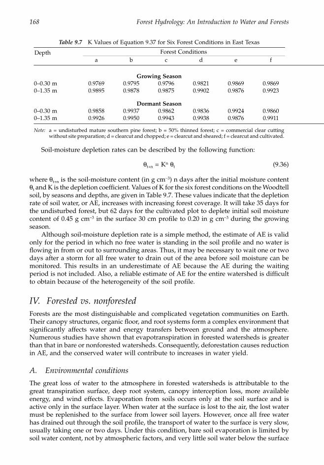
168 Forest Hydrology: An Introduction to Water and Forests
Soil-moisture depletion rates can be described by the following function:
qt+n = Kn qt (9.36)
where qt+n is the soil-moisture content (in g cm-3) n days after the initial moisture contentqt and K is the depletion coefficient. Values of K for the six forest conditions on the Woodtellsoil, by seasons and depths, are given in Table 9.7. These values indicate that the depletionrate of soil water, or AE, increases with increasing forest coverage. It will take 35 days forthe undisturbed forest, but 62 days for the cultivated plot to deplete initial soil moisturecontent of 0.45 g cm-3 in the surface 30 cm profile to 0.20 in g cm-3 during the growingseason.
Although soil-moisture depletion rate is a simple method, the estimate of AE is validonly for the period in which no free water is standing in the soil profile and no water isflowing in from or out to surrounding areas. Thus, it may be necessary to wait one or twodays after a storm for all free water to drain out of the area before soil moisture can bemonitored. This results in an underestimate of AE because the AE during the waitingperiod is not included. Also, a reliable estimate of AE for the entire watershed is difficultto obtain because of the heterogeneity of the soil profile.
IV. Forested vs. nonforestedForests are the most distinguishable and complicated vegetation communities on Earth.Their canopy structures, organic floor, and root systems form a complex environment thatsignificantly affects water and energy transfers between ground and the atmosphere.Numerous studies have shown that evapotranspiration in forested watersheds is greaterthan that in bare or nonforested watersheds. Consequently, deforestation causes reductionin AE, and the conserved water will contribute to increases in water yield.
A. Environmental conditions
The great loss of water to the atmosphere in forested watersheds is attributable to thegreat transpiration surface, deep root system, canopy interception loss, more availableenergy, and wind effects. Evaporation from soils occurs only at the soil surface and isactive only in the surface layer. When water at the surface is lost to the air, the lost watermust be replenished to the surface from lower soil layers. However, once all free waterhas drained out through the soil profile, the transport of water to the surface is very slow,usually taking one or two days. Under this condition, bare soil evaporation is limited bysoil water content, not by atmospheric factors, and very little soil water below the surface
Table 9.7 K Values of Equation 9.37 for Six Forest Conditions in East Texas
Depth Forest Conditionsa b c d e f
Growing Season0–0.30 m 0.9769 0.9795 0.9796 0.9821 0.9869 0.98690–1.35 m 0.9895 0.9878 0.9875 0.9902 0.9876 0.9923
Dormant Season0–0.30 m 0.9858 0.9937 0.9862 0.9836 0.9924 0.98600–1.35 m 0.9926 0.9950 0.9943 0.9938 0.9876 0.9911
Note: a = undisturbed mature southern pine forest; b = 50% thinned forest; c = commercial clear cuttingwithout site preparation; d = clearcut and chopped; e = clearcut and sheared; f = clearcut and cultivated.
1363_C09_fm Page 168 Wednesday, December 4, 2002 7:43 AM
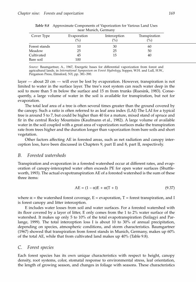
Chapter nine: Forests and vaporization 169
layer — about 20 cm — will ever be lost by evaporation. However, transpiration is notlimited to water in the surface layer. The tree’s root system can reach water deep in thesoil to more than 5 m below the surface and 15 m from trunks (Ruesink, 1983). Conse-quently, a large volume of water in the soil is available for transpiration, but not forevaporation.
The total leaf area of a tree is often several times greater than the ground covered bythe canopy. Such a ratio is often referred to as leaf area index (LAI) The LAI for a typicaltree is around 5 to 7, but could be higher than 40 for a mature, mixed stand of spruce andfir in the central Rocky Mountains (Kaufmann et al., 1982). A large volume of availablewater in the soil coupled with a great area of vaporization surfaces make the transpirationrate from trees higher and the duration longer than vaporization from bare soils and shortvegetation.
Other factors affecting AE in forested areas, such as net radiation and canopy inter-ception loss, have been discussed in Chapters 9, part II and 8, part II, respectively.
B. Forested watersheds
Transpiration and evaporation in a forested watershed occur at different rates, and evap-oration of canopy-intercepted water often exceeds PE for open water surfaces (Shuttle-worth, 1993). The actual evapotranspiration AE of a forested watershed is the sum of thesethree items:
AE = (1 – a)E + a(T + I) (9.37)
where a = the watershed forest coverage, E = evaporation, T = forest transpiration, and Iis forest canopy and litter interception.
E includes water losses from soil and water surfaces. For a forested watershed withits floor covered by a layer of litter, E only comes from the 1 to 2% water surface of thewatershed. It makes up only 5 to 10% of the total evapotranspiration (Szilagyi and Par-lange, 1999). The total interception loss I is about 10 to 30% of annual precipitation,depending on species, atmospheric conditions, and storm characteristics. Baumgartner(1967) showed that transpiration from forest stands in Munich, Germany, makes up 60%of the total AE, while that from cultivated land makes up 40% (Table 9.8).
C. Forest species
Each forest species has its own unique characteristics with respect to height, canopydensity, root systems, color, stomatal response to environmental stress, leaf orientation,the length of growing season, and changes in foliage with seasons. These characteristics
Table 9.8 Approximate Components of Vaporization for Various Land Uses near Munich, Germany
Cover Type Evaporation(%)
Interception(%)
Transpiration(%)
Forest stands 10 30 60Meadow 25 25 50Cultivated 45 15 40Bare soil 100
Source: Baumgartner, A., 1967, Energetic bases for differential vaporization from forest andagricultural lands, in International Symposium on Forest Hydrology, Sopper, W.H. and Lull, H.W.,Pergamon Press, Elmsford, NY, pp. 381–390.
1363_C09_fm Page 169 Wednesday, December 4, 2002 7:43 AM
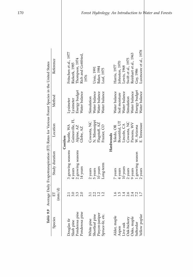
170 Forest Hydrology: An Introduction to Water and Forests
Tabl
e 9.
9A
vera
ge D
aily
Eva
potr
ansp
irat
ion
(ET
) R
ates
for
Var
ious
For
est
Spec
ies
in t
he U
nite
d S
tate
s
Spec
ies
ET
(mm
/d
)St
udy
dur
atio
nL
ocat
ion
Met
hod
Ref
eren
ce
Con
ifer
sD
ougl
as fi
r2.
13
grow
ing
seas
ons
Seat
tle,
WA
Lysi
met
erFr
itsc
hen
et a
l., 1
977
Slas
h pi
ne3.
04
year
sG
aine
svill
e, F
LLy
sim
eter
Rie
kerk
, 198
5Po
nder
osa
pine
3.3
2 gr
owin
g se
ason
sA
lpin
e, A
ZE
nerg
y bu
dge
tT
hom
pson
, 197
4Po
nder
osa
pine
2.0
14 y
ears
Glo
be, A
ZW
ater
bal
ance
Ric
h an
d G
ottf
ried
, 19
76W
hite
pin
e3.
12
year
sC
owee
ta, N
CSi
mul
atio
n
Shor
tlea
f pi
ne2.
25
year
sN
. Mis
siss
ippi
Wat
er b
alan
ceU
rsic
, 199
1Pi
nyon
-juni
per
1.2
10 y
ears
Flag
staf
f, A
ZW
ater
bal
ance
Bak
er, 1
984
Spru
ce-fi
r, et
c.1.
2L
ong-
term
Fraz
ier,
CO
Wat
er b
alan
ceL
eaf,
1975
Har
dw
ood
sA
lder
, map
le1.
67
year
sTo
led
o, O
RW
ater
bal
ance
Har
ris,
197
7A
spen
1.5
4 ye
ars
Bou
ntif
ul, U
TSo
il m
oist
ure
John
ston
, 197
0L
ive
oak
1.4
10 y
ears
Lin
coln
, CA
Wat
er b
alan
ceL
ewis
, 196
8O
ak-h
icko
ry2.
62
year
sC
owee
ta, N
CSi
mul
atio
nSw
ift
et a
l., 1
975
Oak
s, m
aple
2.4
9 ye
ars
Pars
ons,
WV
Wat
er b
alan
ceR
einh
art
et a
l., 1
963
Salt
ced
ar7.
21
grow
ing
seas
onW
. Ari
zona
Ene
rgy
bud
get
Gay
, 198
6Ye
llow
pop
lar
1.7
2 ye
ars
E. T
enne
ssee
Wat
er b
alan
ceL
uxm
oore
et
al.,
1978
1363_C09_fm Page 170 Wednesday, December 4, 2002 7:43 AM
Chapter nine: Forests and vaporization 171
affect the amount of available energy in a forest and the ability of a plant to transpirewater. Large differences in transpiration loss do exist among species. In the central RockyMountains, ratios of annual transpiration for Engelmann spruce, subalpine fir, lodgepolepine, and aspen stands of equal basal area are 3.2, 2.1, 1.8, and 1, respectively (Kaufmann,1985). Thus, total water losses to the atmosphere in forested watersheds are greatly affectedby species composition in the watershed, which leads to watershed forest manipulationresulting in significant alterations of streamflow quantity and regimes around the world(see Chapter 10, part III).
The average daily evapotranspiration (ET) rates (1.2 to 7.2 mm/d) for a few forestspecies in the U.S. are given in Table 9.9. Although direct comparison of these figures isimproper, they do show that species could cause differences in ET by 2 mm/d for conifersand 5 mm/d for hardwoods, and conifers usually have higher ET than hardwoods.However, based on the transpiration rates (0.4 to 1.2 mm/d) from different temperateforests conducted by 19 studies in Europe, Roberts (1999) stated that transpiration ratesare quite similar among species and from day to day. He argued that there is a strongnegative correlation between air humidity deficit and canopy resistance. When waterdemand in the air is high, stomata tend to close, and when the demand is low, the stomataopen. In addition, the transpiration rate for species with higher initial soil-water depletionrates or higher stomatal resistance declines more rapidly as water deficit increases. Allthese cause differences in transpiration rates to be insignificant among species.
Roberts’ (1999) arguments on the atmospheric humidity deficit–leaf resistancedescribes the general function of stomata; but the responses of stomata to humidity deficitare not necessarily the same among species. The decline in transpiration rates may befaster for those species with higher initial transpiration rates and greater stomatal resis-tance, but the total transpiration loss is not necessarily the same. In fact, significantdifferences in transpiration rates among species have been verified by soil moisture deple-tion rates and by vegetation-manipulation studies in many parts of the world. The tran-spiration rates of 0.4 to 1.2 mm/d for those European forests as summarized by Robertsseem to be significantly different among species.
Canopy resistance increases rapidly in the fall as chlorophyll is destroyed and leaveschange color. In the northeastern U.S., leaves of hickory change color 3 to 4 weeks earlierthan leaves of maple and oak, which causes transpiration rates to differ among speciesby several weeks. It is common for canopy resistance to cause differences in daily tran-spiration by 20% among species (Federer and Lash, 1978). Stomata are the biological valvesthat regulate water loss in a plant; their mechanisms in response to environmental stressamong different species and in relation to transpiration require more study.
ReferencesBair, F.E., 1992, Weather of U.S. Cities, 4th ed., Gale Research, Detroit.Baker, M.B., Jr., 1984, Changes in streamflow in an herbicide-treated pinyon-juniper watershed in
Arozona, Water Resour. Res., 20, 1639–1642.Baumgartner, A., 1967, Energetic bases for differential vaporization from forest and agricultural
lands, in International Symposium on Forest Hydrology, Sopper, W.H. and Lull, H.W., PergamonPress, Elmsford, NY, pp. 381–390.
Black, P.E., 1995, Watershed Hydrology Laboratory Manual, Pacific Crest Software, Corvallis, OR.Campbell, G.S., 1977, An Introduction to Environmental Biophysics, Springer-Verlag, Heidelberg.Chang, M., Clendenen, L.D., and Reeves, H.C., 1996, Characteristics of a Humid Climate, Center
for Applied Studies in Forestry, Stephen F. Austin State University, Nacogdoches, TX.Chang, M. et al., 1994, Air and soil temperatures under three forest conditions in East Texas, Texas
J. Sci., 46, 143–155.
1363_C09_fm Page 171 Wednesday, December 4, 2002 7:43 AM
172 Forest Hydrology: An Introduction to Water and Forests
Chang, M., Lee, R., and Dickerson, W.H., 1976, Adequacy of Hydrologic Data for Application inWest Virginia, Bull. #7, WRI-WVU-76–01, Water Res. Inst., West Virginia University, Morgan-town, WV.
Chang, M. et al., 1983, Soil moisture regimes as affected by silvicultural treatments in humid EastTexas, in Hydrology of Humid Tropical Regions with Particular Reference to the Hydrological Effectsof Agricultural and Forestry Practice, IAHS, pp. 175–186.
Dugas, W.A., Bland, W.L., and Arkin, G.F., 1985, Evapotranspiration measurements from different-sized lysimeters, in Advances in Evapotranspiration, Proc. of the National Conf. on Advancesin Evapotranspiration, ASAE, pp. 208–215.
EDS, 1968, Climatic Atlas of the United States, U.S. Dept. of Commerce.Federer, C.A., and Lash, D., 1978, Simulated streamflow response to possible differences in transpi-
ration among species of hardwood trees, Water Resour. Res., 14, 1089–1097.Fritschen, L.J., Hsia, J., and Doraiswamy, P., 1977, Evapotranspiration of a Douglas fir determined
with a weighing lysimeter, Water Resour. Res., 13, 145–148.Fritschen, L.J. and Simpson, J., 1982, A pressure transducer for determining atmospheric pressure
and evaporation with a hydraulic weighing lysimeter, Agr. Meteorol., 26, 273–278.Gardner, W.R., 1959, Solutions of the flow equation for the drying of soils and other porous media,
Soil Sci. Soc. Am. Proc., 23, 183–187.Gay, L.W., 1986, Water use by saltcedar in an arid environment, in Proc. Water Forum 86, Long Beach
Conf., ASAE, pp. 855–862.Hamon, W.R., 1963, Computation of direct runoff amounts from storm rainfall, in Sym. on Theoret-
ical Studies and Practical Methods of Forecasting the Yield of Rivers for Both Long and ShortTerms (Except Floods), Internationall Assoc. Sci. Hydro, pp. 25–62.
Hanks, R.J., 1958, Water vapor transfer in dry soils, Soil Sci. Soc. Am. Proc., 22, 372–374.Hanks, R.J. and Gardner, H.R., 1965, Influence of different diffusivity-water content relations on
evaporation of water from soils, Soil Sci. Soc. Am. Proc., 29, 495–498.Harbeck, G.E., 1962, A Practical Field Technique for Measuring Reservoir Evaporation Utilizing
Mass-Transfer Theory, U.S. Geol. Survey Professional Pap. 272-E, pp. 101–105.Harris, D.D., 1977, Hydrologic changes after logging in two small Oregon coastal watersheds, U.S.
Geological Survey, Water Supply Paper 2037.Harrold, L.L. and Dreibelbis, F.R., 1958, Evaluation of Agricultural Hydrology by Monolith
Lysimeters, U.S. Dept. Agr. Tech. Bull. #1179, U.S. Gov. Printing Office, Washington, D.C.Hillel, D., 1982, Introduction to Soil Physics, Academic Press, New York.Hornbeck, J.W., 1970, The radiant energy budget of clearcut and forest sites in West Virginia, Forest
Sci., 16, 139–45.Idso, S.B. and Jackson, R.D., 1969, Thermal radiation from the atmosphere, J. Geophy. Res., 74,
5397–403.Jalota, S.K. and Prihar, S.S., 1998, Reducing Soil Water Evaporation with Tillage and Straw Mulching,
Iowa State University Press, Ames.Johnston, R.S., 1970, Evapotranspiration from bare, herbaceous, and aspen plots, a check on a former
study, Water Resour. Res., 6, 324–327.Kaufmann, M.R., 1985, Annual transpiration in subalpine forests: large differences among four tree
species, Forest Ecol. Manage., 13, 235–246.Kaufmann, M.R., Edminster, C.E., and Troendle, C.A., 1982, Leaf Area Determination for Subapline
Tree Species in the Central Rocky Mountains, Res. Paper RM-238, USDA Forest Service.Kirkham, R.R., Gee, G.W., and Jones, T.L., 1984, Weighing lysimeters for long-term water balance
in investigations at remote sites, Soil Sci. Am. J., 48, 1203–1205.Leaf, C.F., 1975, Watershed Management in the Central and Southern Rock Mountains: A Summary
of the Status of Our Knowledge by Vegetation Types, Research Paper RM-142, USDA ForestService.
Lee, R., 1980, Forest Hydrology, Columbia University Press, New York.Lewis, D.C., 1968, Annual hydrologic response to watershed conversion from oak woodland to
annual grassland, Water Resour. Res., 4, 59–72.List, R., 1971, Smithsonian Meteorological Tables, Smithsonian Institution Press, 6th revised ed., Wash-
ington, D.C.
1363_C09_fm Page 172 Wednesday, December 4, 2002 7:43 AM
Chapter nine: Forests and vaporization 173
Luxmoore, R.J. et al., 1978, Some measured and simulated plant water relations of yellow poplar,Forest Sci., 24, 327–341.
McCuen, R.H., 1998, Hydrologic Analysis and Design, Prentice Hall, New York.Monteith, J.L., 1965, Evaporation and environment, Sym. Soc. Exp. Biol., 19, 205–234.Monteith, J.L., 1985, Evaporation from land surface: progress in analysis and prediction since 1948,
in Advances in Evapotranspiration, Proc. of the National Conf. on Advances in Evapotranspi-ration, ASAE.
Monteith, J.L. and Unsworth, M.H., 1990, Principles of Environmental Physics, 2nd ed., Edward Arnoldby Routledge, Chapman and Hall, New York.
Peman, H.L., 1948, Natural evaporation from open water, bare-soil polt and grass, Proc. R. Soc.London, A., 193, 120–145.
Penman, H.L., 1963, Vegetation and Hydrology, Tech. Communication No. 53, Commonwealth Agri.Bureaux.
Pruitt, W.O., 1972, Factors affecting potential evapotranspiration, in Biological Effects in the Hydrolog-ical Cycle, Proc., 3rd Int. Seminar Hydrology Professors, UNESCO and Agri. Exp. Sta., PurdueUniversity, West Lafayette, IN, pp. 82–102.
Reinhart, K.G., Eschner, A.R., and Trimble, G.R., Jr., 1963, Effect on Streamflow of Four ForestPractices in the Mountains of West Virginia, Research Paper NE-1, U.S. Forest Service.
Riekerk, H., 1985, Lysimetric measurement of pine evapotranspiration for water balances, in Ad-vances in Evapotranspiration, Proc. National Conf. Advances Evapotranspiration, ASAE, pp.276–281.
Rich, L.R. and Gottfried, G.J., 1976, Water yields resulting from treatments on the Workman CreekExperimental Watershed in central Arizona, Water Resour. Res., 12, 1053–1060.
Roberts, J., 1999, Plants and water in forests and woodlands, in Eco-Hydrology, Baird, A.J. and Wilby,R.L., Eds., Routledge, New York, pp. 181–236.
Ruesink, L.E., 1983, Wanted Water Rustlers, Texas Water Resour. Inst., Texas Agri. Exp. Sta., TAMU,College Station, TX.
Shuttleworth, W.J., 1993, Evaporation, in Handbook of Hydrology, Maidment, D.R., Ed., McGraw-Hill,New York, pp. 4, 1–53.
Swift, L.W., Jr. et al., 1975, Simulation of evapotranspiration and drainage from mature and clear-cut deciduous forests and young pine plantation, Water Resour. Res., 11, 667–73.
Szilagyi, J. and Parlange, M.B., 1999, Defining watershed-scale evaporation using a normalizeddifference vegetation index, J. Am. Water Resour. Assoc., 35, 1245–1255.
Thompson, J.R., 1974, Energy budget measurements over three cover types in eastern Arizona, WaterResour. Res., 10, 1045–1048.
Thornthwaite, C.W., 1948, An approach toward a rational classification of climate, Geogr. Rev., 38,55–94.
Thorthwaite, C.W. and Mather, J.R., 1957, Instructions and Tables for Computing Potential Evapotrans-piration and the Water Balance, Laboratory of Climatology XIX (3), Centerton, NJ.
Ursic, S.J., 1991, Hydrologic effects of two methods of harvesting mature southern pine, Water Resour.Bull., 27, 303–315.
1363_C09_fm Page 173 Wednesday, December 4, 2002 7:43 AM

1363_C09_fm Page 174 Wednesday, December 4, 2002 7:43 AM

175
chapter ten
Forests and streamflow
Contents
I. Runoff generation............................................................................................................176A. Rainfall intensity .....................................................................................................177B. Soil infiltration.........................................................................................................178
1. Soil water............................................................................................................1782. Infiltration capacity ..........................................................................................179
a. The Green-Ampt model.............................................................................179b. The SCS RCN approach.............................................................................182
C. Mechanics of runoff................................................................................................182II. Watershed discharges .....................................................................................................183
A. Hydrograph .............................................................................................................1831. Prominent features ...........................................................................................1832. Direct runoff vs. baseflow ...............................................................................184
B. Factors affecting watershed discharge ................................................................1851. Climate................................................................................................................1852. Topography........................................................................................................1853. Land use .............................................................................................................186
C. Estimation of streamflow ......................................................................................1881. The SCS RCN model (storm runoff volume)...............................................1882. The rational equation (storm peakflow) .......................................................1883. The Manning equation (flood flows).............................................................1904. Water balance approach (annual streamflow) .............................................193
III. Forest practices and water quantity.............................................................................193A. Water yield...............................................................................................................195
1. Forest-cutting intensity ....................................................................................1952. Species.................................................................................................................1973. Precipitation.......................................................................................................1974. Soil topographic conditions ............................................................................199
B. Timing of streamflow.............................................................................................199C. Flow extremes .........................................................................................................200
1. Peak flows ..........................................................................................................2002. Low flows...........................................................................................................2013. Flow duration....................................................................................................201
D. Groundwater ...........................................................................................................2021. Groundwater in steep terrain .........................................................................2022. Groundwater in level terrain..........................................................................203
1363_C10_fm Page 175 Wednesday, December 4, 2002 7:43 AM
176 Forest Hydrology: An Introduction to Water and Forests
IV. Forest practices and water quality ...............................................................................204A. Water-quality determination.................................................................................204
1. Input–output budgets ......................................................................................2042. Water-quality criteria........................................................................................207
B. Forest practices........................................................................................................2071. Clearcutting........................................................................................................2072. Forest roads........................................................................................................2083. Forest fire............................................................................................................2094. Mechanical site preparations ..........................................................................210
C. Cumulative watershed effects ..............................................................................211V. Forest practices and stream habitat .............................................................................212
A. Stream habitat..........................................................................................................2121. Habitat parameters ...........................................................................................213
a. Streamflow ...................................................................................................213b. Temperature .................................................................................................213c. Dissolved oxygen........................................................................................213d. Sediment.......................................................................................................214e. Substrate .......................................................................................................215f. Pools..............................................................................................................215g. Cover.............................................................................................................216
2. Habitat-rating indexes .....................................................................................216B. Forest practices........................................................................................................217
1. On riparian vegetation.....................................................................................2172. On water temperature......................................................................................217
a. Variations......................................................................................................217b. Management ................................................................................................218c. Impacts .........................................................................................................219
3. On sediment ......................................................................................................219a. Variations and impacts ..............................................................................219b. Buffer strips .................................................................................................221
4. On large woody debris ....................................................................................221a. Variations......................................................................................................221b. Impacts .........................................................................................................222
References .....................................................................................................................................222
A body of water moving over Earth’s surface in a network of channels such as brooks,creeks, or rivers is called streamflow, a term that is often interchangeable in use withdischarge or runoff. Water in stream channels comes from one or all of the four components:(1) precipitation intercepted by stream channels, (2) overland flow (surface runoff), (3)interflow (subsurface runoff), and (4) base flow (groundwater runoff). It is the result of theintegral effects of climatic, topographic, geological, soil, and vegetal factors acting upon awatershed system. Thus, streamflow is considered the residual of the hydrologic cycle.
I. Runoff generation
Runoff refers to the portion of precipitation running over the land surface or through thesoil profile to nearby stream channels. When rainfall intensity is greater than soil-infiltra-tion rate, or rainfall amount exceeds soil-infiltration or percolation capacity, runoff occurs.However, many other environmental factors can either reduce the amount of rainfall
1363_C10_fm Page 176 Wednesday, December 4, 2002 7:43 AM
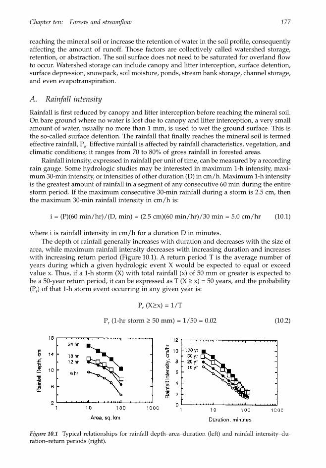
Chapter ten: Forests and streamflow 177
reaching the mineral soil or increase the retention of water in the soil profile, consequentlyaffecting the amount of runoff. Those factors are collectively called watershed storage,retention, or abstraction. The soil surface does not need to be saturated for overland flowto occur. Watershed storage can include canopy and litter interception, surface detention,surface depression, snowpack, soil moisture, ponds, stream bank storage, channel storage,and even evapotranspiration.
A. Rainfall intensity
Rainfall is first reduced by canopy and litter interception before reaching the mineral soil.On bare ground where no water is lost due to canopy and litter interception, a very smallamount of water, usually no more than 1 mm, is used to wet the ground surface. This isthe so-called surface detention. The rainfall that finally reaches the mineral soil is termedeffective rainfall, P
e
. Effective rainfall is affected by rainfall characteristics, vegetation, andclimatic conditions; it ranges from 70 to 80% of gross rainfall in forested areas.
Rainfall intensity, expressed in rainfall per unit of time, can be measured by a recordingrain gauge. Some hydrologic studies may be interested in maximum 1-h intensity, maxi-mum 30-min intensity, or intensities of other duration (D) in cm/h. Maximum 1-h intensityis the greatest amount of rainfall in a segment of any consecutive 60 min during the entirestorm period. If the maximum consecutive 30-min rainfall during a storm is 2.5 cm, thenthe maximum 30-min rainfall intensity in cm/h is:
i = (P)(60 min/hr)/(D, min) = (2.5 cm)(60 min/hr)/30 min = 5.0 cm/hr (10.1)
where i is rainfall intensity in cm/h for a duration D in minutes.The depth of rainfall generally increases with duration and decreases with the size of
area, while maximum rainfall intensity decreases with increasing duration and increaseswith increasing return period (Figure 10.1). A return period T is the average number ofyears during which a given hydrologic event X would be expected to equal or exceedvalue x. Thus, if a 1-h storm (X) with total rainfall (x) of 50 mm or greater is expected tobe a 50-year return period, it can be expressed as T (X
≥
x) = 50 years, and the probability(P
r
) of that 1-h storm event occurring in any given year is:
P
r
(X
≥
x) = 1/T
P
r
(1-hr storm
≥
50 mm) = 1/50 = 0.02 (10.2)
Figure 10.1
Typical relationships for rainfall depth–area–duration (left) and rainfall intensity–du-ration–return periods (right).
1363_C10_fm Page 177 Wednesday, December 4, 2002 7:43 AM
178 Forest Hydrology: An Introduction to Water and Forests
On the other hand, the probability of that event X would not occur in any given year,which is the same as the P
r
for a hydrologic event X equal to or less than x, is:
1 – P
r
(X
≥
x) = (P
r
(X
£
x) = 1 – (1/T) = 1 – 1/50 = 0.98 (10.3)
B. Soil infiltration
Infiltration refers to the entry of water into the soil, a combined process of capillaryattraction and gravitation along with the pressure due to water ponding at the groundsurface. The infiltration rate is high at the initial stage and declines with time as soil voidssuch as animal burrows, root tunnels, interstices, and macro- and micropores graduallyfill with water. It will eventually decline to a constant at which the infiltration rate is equalto the rate of water drained out through the soil profile by gravity. This process of drainingwater to deeper layers is called percolation.
Water movement into and through soil profiles is affected by a variety of factorsreflecting the surface and subsurface conditions and flow characteristics. Surface condi-tions such as type of vegetation cover, land management practices, roughness, crusting,cracking, surface temperature, slope, and chemicals have a significant impact on surfaceponding, overland flow velocity, and ability of the water to enter the soil. Conditionsunder the ground can include soil texture, structure, organic-matter content, depth, com-paction, voids, layering, water content, groundwater table, and root system. These factorsaffect soil water-holding capacity and ability of water movement. For a given soil, theinfiltration in a forest can be many times greater than that over bare ground. Also, infil-tration is greater for warmer water containing less sediment.
1. Soil water
A body of soil consists of solid particles, water solution, and gases. Thus, the total volumeof soil V
t
is the sum of the volumes of solid particles (V
s
), water solution (V
w
), and gases(V
a
):
V
t
= V
s
+ V
w
+ V
a
(10.3)
and the sum of V
w
and V
a
is the total volume of voids or pore spaces. The ratio betweenpore spaces and total soil volume is soil porosity, S
p
:
S
p
= (V
w
+ V
a
)/V
t
(10.4)
Coarse soils have larger but less total volume of spaces and consequently smallerporosity, while fine soils have smaller but more spaces and consequently higher porosity.Thus, the rate of water infiltration is higher, movement is faster, and water-holding capac-ity is smaller for coarse soils. Soil water can be volumetrically expressed by:
q
v
= V
w
/V
t
(10.5)
or gravimetrically expressed by:
q
w
= M
w
/M
s
(10.6)
1363_C10_fm Page 178 Wednesday, December 4, 2002 7:43 AM
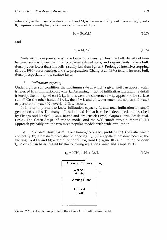
Chapter ten: Forests and streamflow 179
where M
w
is the mass of water content and M
s
is the mass of dry soil. Converting
q
w
into
q
v
requires a multiplier, bulk density of the soil d
b
, or:
q
v
= (
q
w
)(d
b
) (10.7)
and
d
b
= M
s
/V
t
(10.8)
Soils with more pore spaces have lower bulk density. Thus, the bulk density of fine-textured soils is lower than that of coarse-textured soils, and organic soils have a bulkdensity even lower than fine soils, usually less than 1 g/cm
3
. Prolonged intensive cropping(Brady, 1990), forest cutting, and site preparation (Chang et al., 1994) tend to increase bulkdensity, especially in the surface layer.
2. Infiltration capacity
Under a given soil condition, the maximum rate at which a given soil can absorb wateris referred to as infiltration capacity, f
m
. Assuming f = actual infiltration rate and i = rainfallintensity, then f = f
m
when i
≥
f
m
. In this case the difference i – f
m
appears to be surfacerunoff. On the other hand, if i
<
f
m
, then f = i, and all water enters the soil as soil wateror percolation water. No overland flow occurs.
It is often important to know infiltration capacity f
m
and total infiltration in runoffgeneration studies. The many infiltration models that have been developed are describedby Skaggs and Khaleel (1982), Rawls and Brakensiek (1983), Gupta (1989), Rawls et al.(1993). The Green-Ampt infiltration model and the SCS runoff curve number (RCN)approach probably are the two most popular models with wide application.
a. The Green-Ampt model.
For a homogeneous soil profile with (1) an initial watercontent
q
i
, (2) a pressure head due to ponding H
o
, (3) a capillary pressure head at thewetting front H
f
, and (4) a depth to the wetting front L (Figure 10.2), infiltration capacityf
m
in cm/h can be estimated by the following equation (Green and Ampt, 1911):
f
m
= K(H
o
+ H
f
+ L)/L (10.9)
Figure 10.2
Soil moisture profile in the Green-Ampt infiltration model.
1363_C10_fm Page 179 Wednesday, December 4, 2002 7:43 AM
180 Forest Hydrology: An Introduction to Water and Forests
where K is saturated hydraulic conductivity in cm/sec, and H
o
, H
f
, and L are in cm. Thesum of H
o
, H
f
, and L is the total hydraulic head H. Since the change in ratio between Hand L or (
D
H)/(
D
L) is the hydraulic gradient, Equation 10.9 is an application of Darcy’slaw for the velocity of flow V through an unsaturated soil:
V = K (10.10)
Assuming the ponding head is close to zero and the total infiltration (in cm) for aspecific period is F or F = (
q
s
-
q
i
)L, then Equation 10.9 can be rearranged to become:
f
m
= K[1 + (
q
s
–
q
i
)H
f
/F] (10.11)
f
m
= K[1 + N
s
/F] (10.12)
where
q
s
is the saturated soil-water content, a value analogues to the soil porosity but indifferent units (g cm
–3
vs. %), the difference (
q
s
-
q
i
) is the soil-water saturation deficit,and N
s
is the effective capillary pressure head (in cm) and is equal to (
q
s
-
q
i
)H
f
. Theparameter
q
s
can be estimated by (Kidwell et al., 1997):
q
s
= 0.9(1 – d
b
/2.65) (10.13)
where d
b
is the soil bulk density (g cm
-
3
) and 2.65 is the particle density in g cm
-
3
for mostsoils. The integration of Equation 10.12 provides an estimate of cumulative infiltration fora time period t as:
(K) (t) = F – N
s
ln (1 + F/N
s
) (10.14)
In summary, under a steady rainfall condition, infiltration can be treated at three stagesof time t, i.e., before surface ponding, at ponding t
p
, and after ponding:
1. From the beginning to surface ponding, or t < t
p
, the actual infiltration rate is equalto the rainfall intensity (f = i) and the cumulative infiltration is equal to cumulativerainfall, F =
S
(f
¥
t) =
S
(i
¥
t).2. At the time of ponding, or t = t
p
, actual infiltration rate is the infiltration capacityand is equal to the rainfall intensity (f = f
m
= i). The cumulative infiltration atponding F
p
can be calculated by substituting i for f
m
in Equation 10.12 and isrearranged to become:
F
p
= (10.15)
t
p
= (10.16)
3. For the time beyond ponding, or t > t
p
, the infiltration capacity f
m
is calculated byEquation 10.12 and the cumulative infiltration can be calculated by the followingequation (Mein and Larson, 1971; Skaggs and Khaleel, 1982):
K(t – t
p
+ t’
p
) = F – N
s
ln[1 + F/N
s
] (10.17)
DHDL---------
Ns
i/K( ) 1–-----------------------
Fp
i-----
1363_C10_fm Page 180 Wednesday, December 4, 2002 7:43 AM
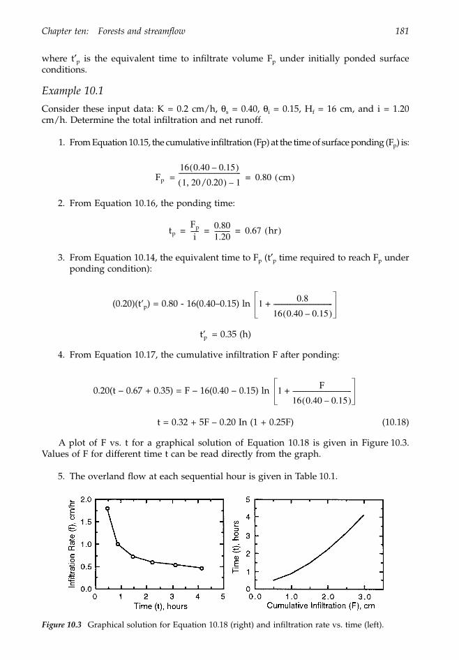
Chapter ten: Forests and streamflow 181
where t¢p is the equivalent time to infiltrate volume Fp under initially ponded surfaceconditions.
Example 10.1
Consider these input data: K = 0.2 cm/h, qs = 0.40, qi = 0.15, Hf = 16 cm, and i = 1.20cm/h. Determine the total infiltration and net runoff.
1. From Equation 10.15, the cumulative infiltration (Fp) at the time of surface ponding (Fp) is:
2. From Equation 10.16, the ponding time:
3. From Equation 10.14, the equivalent time to Fp (t¢p time required to reach Fp underponding condition):
(0.20)(t’p) = 0.80 - 16(0.40–0.15) ln
t’p = 0.35 (h)
4. From Equation 10.17, the cumulative infiltration F after ponding:
0.20(t – 0.67 + 0.35) = F – 16(0.40 – 0.15) ln
t = 0.32 + 5F – 0.20 In (1 + 0.25F) (10.18)
A plot of F vs. t for a graphical solution of Equation 10.18 is given in Figure 10.3.Values of F for different time t can be read directly from the graph.
5. The overland flow at each sequential hour is given in Table 10.1.
Figure 10.3 Graphical solution for Equation 10.18 (right) and infiltration rate vs. time (left).
Fp = 16 0.40 0.15–( )1 20/0.20,( ) 1–
---------------------------------------- 0.80 cm( )=
tpFp
i----- 0.80
1.20---------- 0.67 hr( )= = =
1 0.8
16 0.40 0.15–( )--------------------------------------+
1 F
16 0.40 0.15–( )--------------------------------------+
1363_C10_fm Page 181 Wednesday, December 4, 2002 7:43 AM
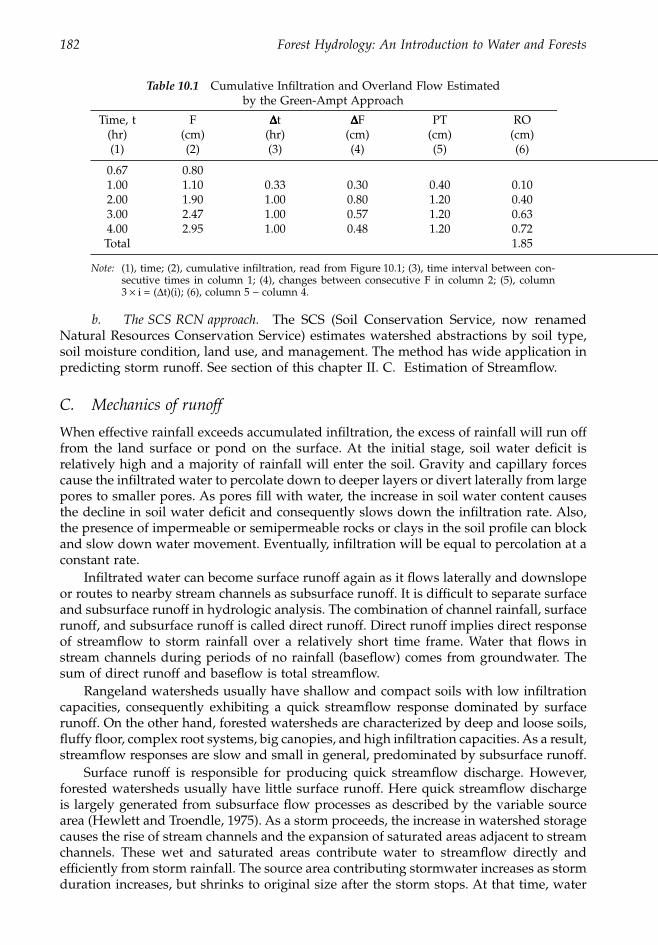
182 Forest Hydrology: An Introduction to Water and Forests
b. The SCS RCN approach. The SCS (Soil Conservation Service, now renamedNatural Resources Conservation Service) estimates watershed abstractions by soil type,soil moisture condition, land use, and management. The method has wide application inpredicting storm runoff. See section of this chapter II. C. Estimation of Streamflow.
C. Mechanics of runoff
When effective rainfall exceeds accumulated infiltration, the excess of rainfall will run offfrom the land surface or pond on the surface. At the initial stage, soil water deficit isrelatively high and a majority of rainfall will enter the soil. Gravity and capillary forcescause the infiltrated water to percolate down to deeper layers or divert laterally from largepores to smaller pores. As pores fill with water, the increase in soil water content causesthe decline in soil water deficit and consequently slows down the infiltration rate. Also,the presence of impermeable or semipermeable rocks or clays in the soil profile can blockand slow down water movement. Eventually, infiltration will be equal to percolation at aconstant rate.
Infiltrated water can become surface runoff again as it flows laterally and downslopeor routes to nearby stream channels as subsurface runoff. It is difficult to separate surfaceand subsurface runoff in hydrologic analysis. The combination of channel rainfall, surfacerunoff, and subsurface runoff is called direct runoff. Direct runoff implies direct responseof streamflow to storm rainfall over a relatively short time frame. Water that flows instream channels during periods of no rainfall (baseflow) comes from groundwater. Thesum of direct runoff and baseflow is total streamflow.
Rangeland watersheds usually have shallow and compact soils with low infiltrationcapacities, consequently exhibiting a quick streamflow response dominated by surfacerunoff. On the other hand, forested watersheds are characterized by deep and loose soils,fluffy floor, complex root systems, big canopies, and high infiltration capacities. As a result,streamflow responses are slow and small in general, predominated by subsurface runoff.
Surface runoff is responsible for producing quick streamflow discharge. However,forested watersheds usually have little surface runoff. Here quick streamflow dischargeis largely generated from subsurface flow processes as described by the variable sourcearea (Hewlett and Troendle, 1975). As a storm proceeds, the increase in watershed storagecauses the rise of stream channels and the expansion of saturated areas adjacent to streamchannels. These wet and saturated areas contribute water to streamflow directly andefficiently from storm rainfall. The source area contributing stormwater increases as stormduration increases, but shrinks to original size after the storm stops. At that time, water
Table 10.1 Cumulative Infiltration and Overland Flow Estimated by the Green-Ampt Approach
Time, t(hr)(1)
F(cm)(2)
DDDDt(hr)(3)
DDDDF(cm)(4)
PT(cm)(5)
RO(cm)(6)
0.67 0.801.00 1.10 0.33 0.30 0.40 0.102.00 1.90 1.00 0.80 1.20 0.403.00 2.47 1.00 0.57 1.20 0.634.00 2.95 1.00 0.48 1.20 0.72Total 1.85
Note: (1), time; (2), cumulative infiltration, read from Figure 10.1; (3), time interval between con-secutive times in column 1; (4), changes between consecutive F in column 2; (5), column3 ¥ i = (Dt)(i); (6), column 5 - column 4.
1363_C10_fm Page 182 Wednesday, December 4, 2002 7:43 AM
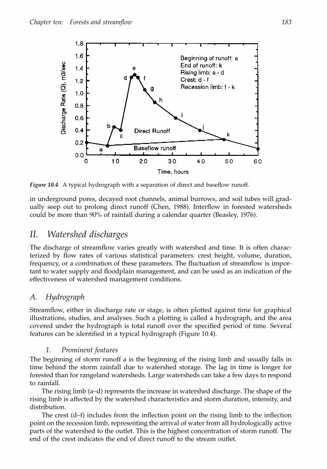
Chapter ten: Forests and streamflow 183
in underground pores, decayed root channels, animal burrows, and soil tubes will grad-ually seep out to prolong direct runoff (Chen, 1988). Interflow in forested watershedscould be more than 90% of rainfall during a calendar quarter (Beasley, 1976).
II. Watershed dischargesThe discharge of streamflow varies greatly with watershed and time. It is often charac-terized by flow rates of various statistical parameters: crest height, volume, duration,frequency, or a combination of these parameters. The fluctuation of streamflow is impor-tant to water supply and floodplain management, and can be used as an indication of theeffectiveness of watershed management conditions.
A. Hydrograph
Streamflow, either in discharge rate or stage, is often plotted against time for graphicalillustrations, studies, and analyses. Such a plotting is called a hydrograph, and the areacovered under the hydrograph is total runoff over the specified period of time. Severalfeatures can be identified in a typical hydrograph (Figure 10.4).
1. Prominent featuresThe beginning of storm runoff a is the beginning of the rising limb and usually falls intime behind the storm rainfall due to watershed storage. The lag in time is longer forforested than for rangeland watersheds. Large watersheds can take a few days to respondto rainfall.
The rising limb (a–d) represents the increase in watershed discharge. The shape of therising limb is affected by the watershed characteristics and storm duration, intensity, anddistribution.
The crest (d–f) includes from the inflection point on the rising limb to the inflectionpoint on the recession limb, representing the arrival of water from all hydrologically activeparts of the watershed to the outlet. This is the highest concentration of storm runoff. Theend of the crest indicates the end of direct runoff to the stream outlet.
Figure 10.4 A typical hydrograph with a separation of direct and baseflow runoff.
1363_C10_fm Page 183 Wednesday, December 4, 2002 7:43 AM
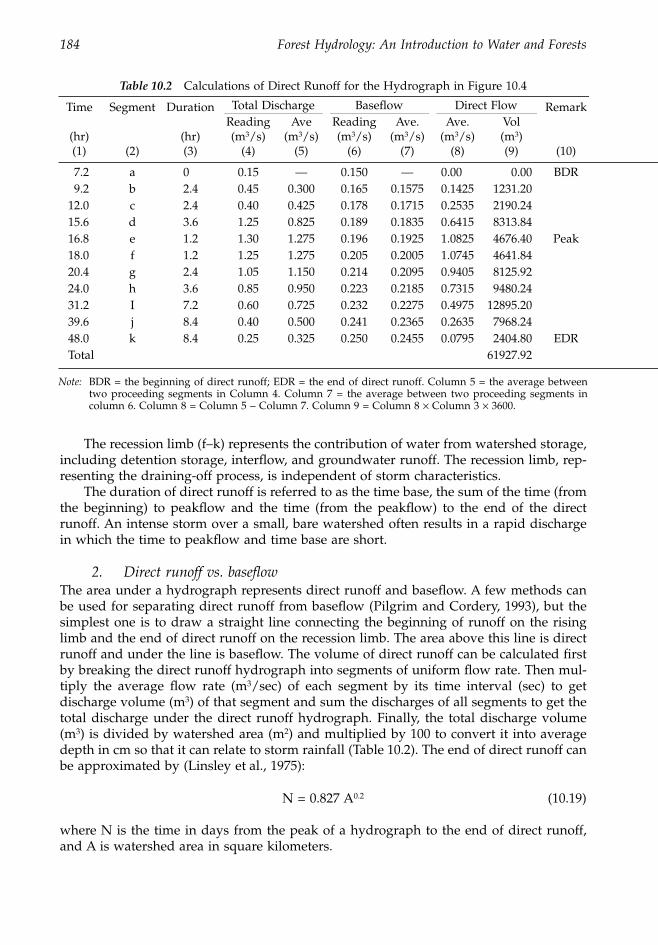
184 Forest Hydrology: An Introduction to Water and Forests
The recession limb (f–k) represents the contribution of water from watershed storage,including detention storage, interflow, and groundwater runoff. The recession limb, rep-resenting the draining-off process, is independent of storm characteristics.
The duration of direct runoff is referred to as the time base, the sum of the time (fromthe beginning) to peakflow and the time (from the peakflow) to the end of the directrunoff. An intense storm over a small, bare watershed often results in a rapid dischargein which the time to peakflow and time base are short.
2. Direct runoff vs. baseflowThe area under a hydrograph represents direct runoff and baseflow. A few methods canbe used for separating direct runoff from baseflow (Pilgrim and Cordery, 1993), but thesimplest one is to draw a straight line connecting the beginning of runoff on the risinglimb and the end of direct runoff on the recession limb. The area above this line is directrunoff and under the line is baseflow. The volume of direct runoff can be calculated firstby breaking the direct runoff hydrograph into segments of uniform flow rate. Then mul-tiply the average flow rate (m3/sec) of each segment by its time interval (sec) to getdischarge volume (m3) of that segment and sum the discharges of all segments to get thetotal discharge under the direct runoff hydrograph. Finally, the total discharge volume(m3) is divided by watershed area (m2) and multiplied by 100 to convert it into averagedepth in cm so that it can relate to storm rainfall (Table 10.2). The end of direct runoff canbe approximated by (Linsley et al., 1975):
N = 0.827 A0.2 (10.19)
where N is the time in days from the peak of a hydrograph to the end of direct runoff,and A is watershed area in square kilometers.
Table 10.2 Calculations of Direct Runoff for the Hydrograph in Figure 10.4
Time
(hr)(1)
Segment
(2)
Duration
(hr)(3)
Total Discharge Baseflow Direct Flow Remark
(10)
Reading(m3/s)
(4)
Ave(m3/s)
(5)
Reading(m3/s)
(6)
Ave.(m3/s)
(7)
Ave.(m3/s)
(8)
Vol(m3)(9)
7.2 a 0 0.15 — 0.150 — 0.00 0.00 BDR9.2 b 2.4 0.45 0.300 0.165 0.1575 0.1425 1231.20
12.0 c 2.4 0.40 0.425 0.178 0.1715 0.2535 2190.2415.6 d 3.6 1.25 0.825 0.189 0.1835 0.6415 8313.8416.8 e 1.2 1.30 1.275 0.196 0.1925 1.0825 4676.40 Peak18.0 f 1.2 1.25 1.275 0.205 0.2005 1.0745 4641.8420.4 g 2.4 1.05 1.150 0.214 0.2095 0.9405 8125.9224.0 h 3.6 0.85 0.950 0.223 0.2185 0.7315 9480.2431.2 I 7.2 0.60 0.725 0.232 0.2275 0.4975 12895.2039.6 j 8.4 0.40 0.500 0.241 0.2365 0.2635 7968.2448.0 k 8.4 0.25 0.325 0.250 0.2455 0.0795 2404.80 EDRTotal 61927.92
Note: BDR = the beginning of direct runoff; EDR = the end of direct runoff. Column 5 = the average betweentwo proceeding segments in Column 4. Column 7 = the average between two proceeding segments incolumn 6. Column 8 = Column 5 - Column 7. Column 9 = Column 8 ¥ Column 3 ¥ 3600.
1363_C10_fm Page 184 Wednesday, December 4, 2002 7:43 AM
Chapter ten: Forests and streamflow 185
B. Factors affecting watershed discharge
Like rainfall, streamflow fluctuates with time within watersheds in response to watershedclimate, topography, and land-use conditions.
1. ClimatePrecipitation is the input in the hydrologic system. Its intensity, depth, duration, type,distribution within the watershed, and direction of storm movement impose direct andsignificant impacts to streamflow regimes and hydrograph shape. For a given duration,the hydrograph produced from storms of greater intensity will exhibit a higher peakflowand a greater runoff volume. A storm that occurs near the watershed outlet will result ina rapid rise and sharp peakflow. On the other hand, the hydrograph will exhibit a longertime base, lower peakflow, and slower rise to peak if the storm occurs in the upper partsof the watershed. In general, snowmelt tends to exhibit a lower and broader runoffhydrograph than rainfall.
Lower atmospheric humidity, higher air temperature, solar radiation, and wind speedtend to increase evapotranspiration and reduce water available for runoff. As a result,streamflow generally decreases with air temperature and increases with rainfall as illus-trated by an empirical equation for estimating annual streamflow (Q, mm) for the 80 km2
La Nana Creek watershed in Nacogdoches, east Texas (Chang and Sayok, 1990):
Q = –396.16 + 194.23 (Pt/T2) (10.20)
where Pt is annual rainfall in mm and T is annual air temperature in ∞C.In areas where snow is the major type of precipitation, a sudden rise in air temperature
in early spring often causes rapid melting of snowpacks, which can result in devastatingfloods (Chang and Lee, 1976).
2. TopographyWatershed topography can be characterized by a variety of parameters such as slope,shape, elevation, size, relief ratio, stream density and frequency, and many others (Changand Boyer, 1977; Chang, 1982). They affect streamflow and influence the shape of thehydrograph through watershed storage, runoff speed, infiltration, and soil water content.A watershed with higher elevations implies lower temperature, less evapotranspiration,greater rainfall, steeper slope, and shallower soil depth, which lead to produce morerunoff. A steep slope can make overland runoff greater and faster and soil infiltrationlower.
The hydrologic behavior of small watersheds tends to be different from that of largewatersheds. A small watershed is very sensitive to high-intensity rainfall of short durationand land use. Thus, overland flow is a dominating factor affecting the peakflow, and thestreamflow hydrograph is characterized by a sharp rise to peakflow and a rapid fall inrecession. In large watersheds, the average watershed slope, chances for a single storm tocover the entire watershed, and the average storm depth and intensity are smaller. Thus,the streamflow hydrograph is dominated by watershed and channel storage, and it exhibitsa broader crest and longer time base (Figure 10.5).
The positive effects of watershed area A (km2) on streamflow Q (m3/sec) leads itperhaps to be the most widely used topographic parameter in hydrologic analyses (Gin-gras et al., 1994):
Q = aAb (10.21)
1363_C10_fm Page 185 Wednesday, December 4, 2002 7:43 AM
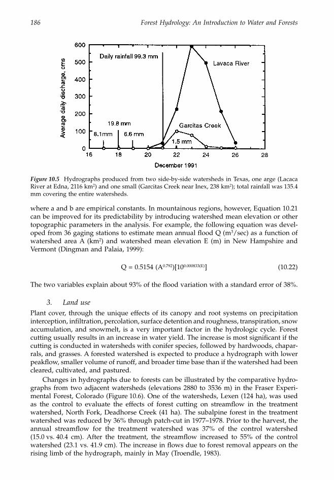
186 Forest Hydrology: An Introduction to Water and Forests
where a and b are empirical constants. In mountainous regions, however, Equation 10.21can be improved for its predictability by introducing watershed mean elevation or othertopographic parameters in the analysis. For example, the following equation was devel-oped from 36 gaging stations to estimate mean annual flood Q (m3/sec) as a function ofwatershed area A (km2) and watershed mean elevation E (m) in New Hampshire andVermont (Dingman and Palaia, 1999):
Q = 0.5154 (A0.792)[100.000833(E)] (10.22)
The two variables explain about 93% of the flood variation with a standard error of 38%.
3. Land usePlant cover, through the unique effects of its canopy and root systems on precipitationinterception, infiltration, percolation, surface detention and roughness, transpiration, snowaccumulation, and snowmelt, is a very important factor in the hydrologic cycle. Forestcutting usually results in an increase in water yield. The increase is most significant if thecutting is conducted in watersheds with conifer species, followed by hardwoods, chapar-rals, and grasses. A forested watershed is expected to produce a hydrograph with lowerpeakflow, smaller volume of runoff, and broader time base than if the watershed had beencleared, cultivated, and pastured.
Changes in hydrographs due to forests can be illustrated by the comparative hydro-graphs from two adjacent watersheds (elevations 2880 to 3536 m) in the Fraser Experi-mental Forest, Colorado (Figure 10.6). One of the watersheds, Lexen (124 ha), was usedas the control to evaluate the effects of forest cutting on streamflow in the treatmentwatershed, North Fork, Deadhorse Creek (41 ha). The subalpine forest in the treatmentwatershed was reduced by 36% through patch-cut in 1977–1978. Prior to the harvest, theannual streamflow for the treatment watershed was 37% of the control watershed(15.0 vs. 40.4 cm). After the treatment, the streamflow increased to 55% of the controlwatershed (23.1 vs. 41.9 cm). The increase in flows due to forest removal appears on therising limb of the hydrograph, mainly in May (Troendle, 1983).
Figure 10.5 Hydrographs produced from two side-by-side watersheds in Texas, one arge (LacacaRiver at Edna, 2116 km2) and one small (Garcitas Creek near Inex, 238 km2); total rainfall was 135.4mm covering the entire watersheds.
1363_C10_fm Page 186 Wednesday, December 4, 2002 7:43 AM
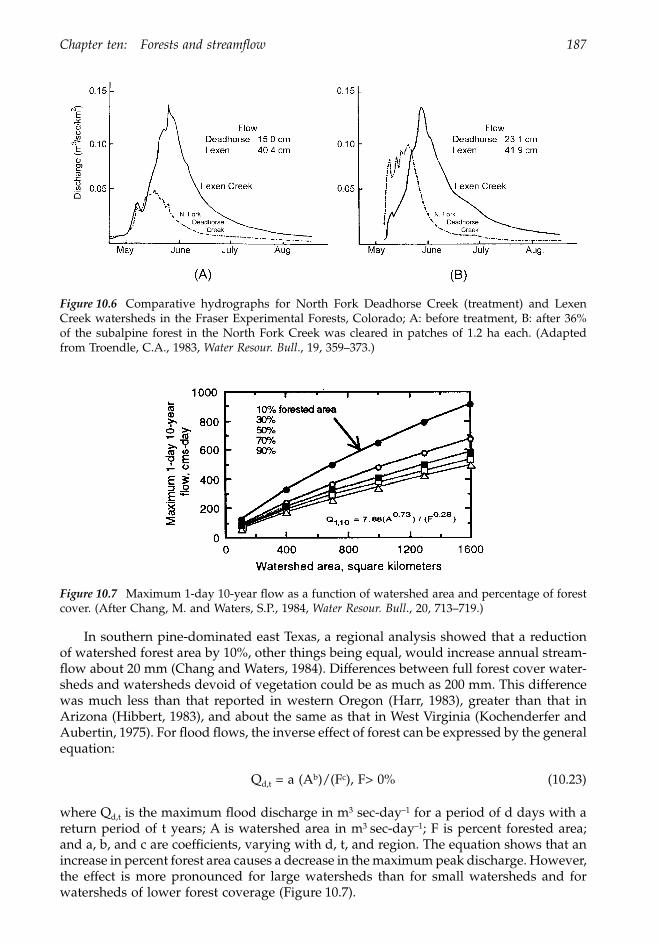
Chapter ten: Forests and streamflow 187
In southern pine-dominated east Texas, a regional analysis showed that a reductionof watershed forest area by 10%, other things being equal, would increase annual stream-flow about 20 mm (Chang and Waters, 1984). Differences between full forest cover water-sheds and watersheds devoid of vegetation could be as much as 200 mm. This differencewas much less than that reported in western Oregon (Harr, 1983), greater than that inArizona (Hibbert, 1983), and about the same as that in West Virginia (Kochenderfer andAubertin, 1975). For flood flows, the inverse effect of forest can be expressed by the generalequation:
Qd,t = a (Ab)/(Fc), F> 0% (10.23)
where Qd,t is the maximum flood discharge in m3 sec-day–1 for a period of d days with areturn period of t years; A is watershed area in m3 sec-day–1; F is percent forested area;and a, b, and c are coefficients, varying with d, t, and region. The equation shows that anincrease in percent forest area causes a decrease in the maximum peak discharge. However,the effect is more pronounced for large watersheds than for small watersheds and forwatersheds of lower forest coverage (Figure 10.7).
Figure 10.6 Comparative hydrographs for North Fork Deadhorse Creek (treatment) and LexenCreek watersheds in the Fraser Experimental Forests, Colorado; A: before treatment, B: after 36%of the subalpine forest in the North Fork Creek was cleared in patches of 1.2 ha each. (Adaptedfrom Troendle, C.A., 1983, Water Resour. Bull., 19, 359–373.)
Figure 10.7 Maximum 1-day 10-year flow as a function of watershed area and percentage of forestcover. (After Chang, M. and Waters, S.P., 1984, Water Resour. Bull., 20, 713–719.)
1363_C10_fm Page 187 Wednesday, December 4, 2002 7:43 AM
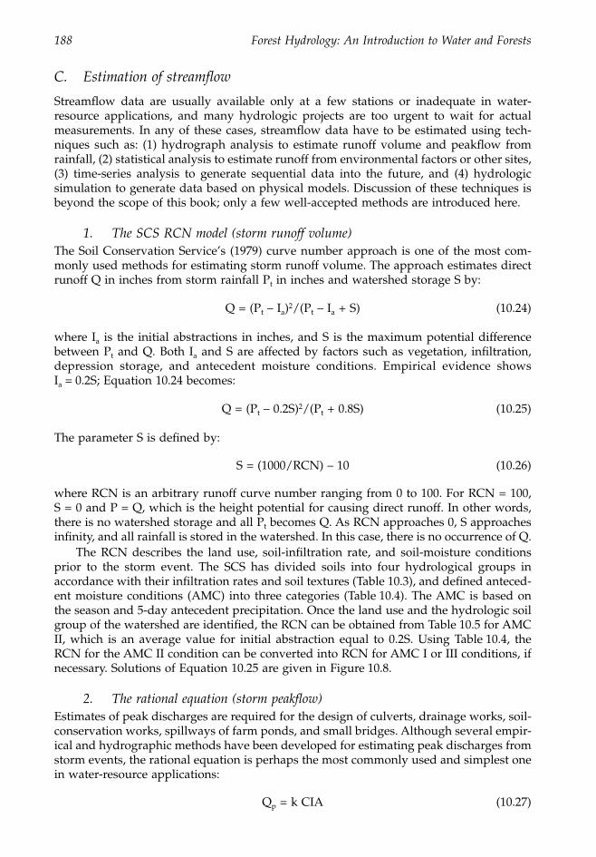
188 Forest Hydrology: An Introduction to Water and Forests
C. Estimation of streamflow
Streamflow data are usually available only at a few stations or inadequate in water-resource applications, and many hydrologic projects are too urgent to wait for actualmeasurements. In any of these cases, streamflow data have to be estimated using tech-niques such as: (1) hydrograph analysis to estimate runoff volume and peakflow fromrainfall, (2) statistical analysis to estimate runoff from environmental factors or other sites,(3) time-series analysis to generate sequential data into the future, and (4) hydrologicsimulation to generate data based on physical models. Discussion of these techniques isbeyond the scope of this book; only a few well-accepted methods are introduced here.
1. The SCS RCN model (storm runoff volume)The Soil Conservation Service’s (1979) curve number approach is one of the most com-monly used methods for estimating storm runoff volume. The approach estimates directrunoff Q in inches from storm rainfall Pt in inches and watershed storage S by:
Q = (Pt – Ia)2/(Pt – Ia + S) (10.24)
where Ia is the initial abstractions in inches, and S is the maximum potential differencebetween Pt and Q. Both Ia and S are affected by factors such as vegetation, infiltration,depression storage, and antecedent moisture conditions. Empirical evidence showsIa = 0.2S; Equation 10.24 becomes:
Q = (Pt – 0.2S)2/(Pt + 0.8S) (10.25)
The parameter S is defined by:
S = (1000/RCN) – 10 (10.26)
where RCN is an arbitrary runoff curve number ranging from 0 to 100. For RCN = 100,S = 0 and P = Q, which is the height potential for causing direct runoff. In other words,there is no watershed storage and all Pt becomes Q. As RCN approaches 0, S approachesinfinity, and all rainfall is stored in the watershed. In this case, there is no occurrence of Q.
The RCN describes the land use, soil-infiltration rate, and soil-moisture conditionsprior to the storm event. The SCS has divided soils into four hydrological groups inaccordance with their infiltration rates and soil textures (Table 10.3), and defined anteced-ent moisture conditions (AMC) into three categories (Table 10.4). The AMC is based onthe season and 5-day antecedent precipitation. Once the land use and the hydrologic soilgroup of the watershed are identified, the RCN can be obtained from Table 10.5 for AMCII, which is an average value for initial abstraction equal to 0.2S. Using Table 10.4, theRCN for the AMC II condition can be converted into RCN for AMC I or III conditions, ifnecessary. Solutions of Equation 10.25 are given in Figure 10.8.
2. The rational equation (storm peakflow)Estimates of peak discharges are required for the design of culverts, drainage works, soil-conservation works, spillways of farm ponds, and small bridges. Although several empir-ical and hydrographic methods have been developed for estimating peak discharges fromstorm events, the rational equation is perhaps the most commonly used and simplest onein water-resource applications:
Qp = k CIA (10.27)
1363_C10_fm Page 188 Wednesday, December 4, 2002 7:43 AM
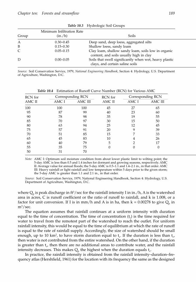
Chapter ten: Forests and streamflow 189
where Qp is peak discharge in ft3/sec for the rainfall intensity I in in./h, A is the watershedarea in acres, C is runoff coefficient or the ratio of runoff to rainfall, and k is 1.008, or afactor for unit conversion. If I is in mm/h and A is in ha, then k = 0.00278 to give Qp inm3/sec.
The equation assumes that rainfall continues at a uniform intensity with durationequal to the time of concentration. The time of concentration (tc) is the time required forwater to travel from the remotest part of the watershed to reach the outlet. For uniformrainfall intensity, this would be equal to the time of equilibrium at which the rate of runoffis equal to the rate of rainfall supply. Accordingly, the size of watershed should be smallenough, up to 10 km2, to have storm duration equal to tc. If the duration is less than tc,then water is not contributed from the entire watershed. On the other hand, if the durationis greater than tc, then there are no additional areas to contribute water, and the rainfallintensity decreases. This makes Qp the highest when the duration equals tc.
In practice, the rainfall intensity is obtained from the rainfall intensity–duration–fre-quency atlas (Hershfield, 1961) for the location with its frequency the same as the designed
Table 10.3 Hydrologic Soil Groups
GroupMinimum Infiltration Rate
(in./h) Soils
A 0.30–0.45 Deep sand, deep loess, aggregated siltsB 0.15–0.30 Shallow loess, sandy loamC 0.05–0.15 Clay loam, shallow sandy loam, soils low in organic
content, and soils usually high in clayD 0.00–0.05 Soils that swell significantly when wet, heavy plastic
clays, and certain saline soils
Source: Soil Conservation Service, 1979, National Engineering Handbook, Section 4: Hydrology, U.S. Departmentof Agriculture, Washington, D.C.
Table 10.4 Estimation of Runoff Curve Number (RCN) for Various AMC
RCN for AMC II
Corresponding RCN RCN for AMC II
Corresponding RCNAMC I AMC III AMC I AMC III
100 100 100 45 27 6595 87 99 40 23 6090 78 98 35 19 5585 70 97 30 15 5080 63 94 25 12 4575 57 91 20 9 3970 51 85 15 7 3365 45 83 10 4 2660 40 79 5 2 1755 35 75 0 0 050 31 70
Note: AMC I: Optimum soil moisture condition from about lower plastic limit to wilting point; the5-day AMC is less than 0.5 and 1.4 inches for dormant and growing seasons, respectively. AMCII: Average value for annual floods; the 5-day AMC is 0.5–1.1 and 1.4–2.1 in., in that order. AMCIII: Heavy rainfall or light rainfall and low temperature within 5 days prior to the given storm;the 5-day AMC is greater than 1.1 and 2.1 in., in that order.
Source: Soil Conservation Service, 1979, National Engineering Handbook, Section 4: Hydrology, U.S.Department of Agriculture, Washington, D.C.
1363_C10_fm Page 189 Wednesday, December 4, 2002 7:43 AM
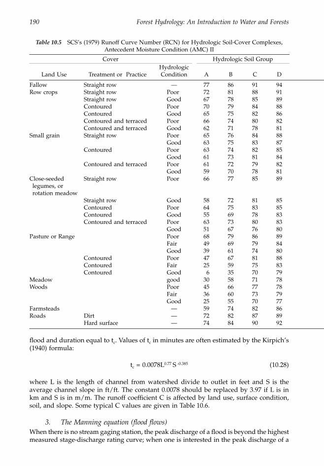
190 Forest Hydrology: An Introduction to Water and Forests
flood and duration equal to tc. Values of tc in minutes are often estimated by the Kirpich’s(1940) formula:
tc = 0.0078L0.77 S -0.385 (10.28)
where L is the length of channel from watershed divide to outlet in feet and S is theaverage channel slope in ft/ft. The constant 0.0078 should be replaced by 3.97 if L is inkm and S is in m/m. The runoff coefficient C is affected by land use, surface condition,soil, and slope. Some typical C values are given in Table 10.6.
3. The Manning equation (flood flows)When there is no stream gaging station, the peak discharge of a flood is beyond the highestmeasured stage-discharge rating curve; when one is interested in the peak discharge of a
Table 10.5 SCS’s (1979) Runoff Curve Number (RCN) for Hydrologic Soil-Cover Complexes, Antecedent Moisture Condition (AMC) II
Cover Hydrologic Soil Group
Land Use Treatment or PracticeHydrologic Condition A B C D
Fallow Straight row — 77 86 91 94Row crops Straight row Poor 72 81 88 91
Straight row Good 67 78 85 89Contoured Poor 70 79 84 88Contoured Good 65 75 82 86Contoured and terraced Poor 66 74 80 82Contoured and terraced Good 62 71 78 81
Small grain Straight row Poor 65 76 84 88Good 63 75 83 87
Contoured Poor 63 74 82 85Good 61 73 81 84
Contoured and terraced Poor 61 72 79 82Good 59 70 78 81
Close-seeded legumes, or rotation meadow
Straight row Poor 66 77 85 89
Straight row Good 58 72 81 85Contoured Poor 64 75 83 85Contoured Good 55 69 78 83Contoured and terraced Poor 63 73 80 83
Good 51 67 76 80Pasture or Range Poor 68 79 86 89
Fair 49 69 79 84Good 39 61 74 80
Contoured Poor 47 67 81 88Contoured Fair 25 59 75 83Contoured Good 6 35 70 79
Meadow good 30 58 71 78Woods Poor 45 66 77 78
Fair 36 60 73 79Good 25 55 70 77
Farmsteads — 59 74 82 86Roads Dirt — 72 82 87 89
Hard surface — 74 84 90 92
1363_C10_fm Page 190 Wednesday, December 4, 2002 7:43 AM
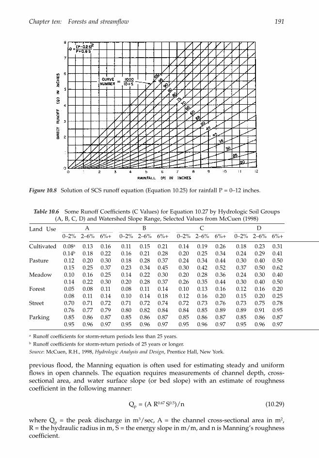
Chapter ten: Forests and streamflow 191
previous flood, the Manning equation is often used for estimating steady and uniformflows in open channels. The equation requires measurements of channel depth, cross-sectional area, and water surface slope (or bed slope) with an estimate of roughnesscoefficient in the following manner:
Qp = (A R0.67 S0.5)/n (10.29)
where Qp = the peak discharge in m3/sec, A = the channel cross-sectional area in m2,R = the hydraulic radius in m, S = the energy slope in m/m, and n is Manning’s roughnesscoefficient.
Figure 10.8 Solution of SCS runoff equation (Equation 10.25) for rainfall P = 0–12 inches.
Table 10.6 Some Runoff Coefficients (C Values) for Equation 10.27 by Hydrologic Soil Groups (A, B, C, D) and Watershed Slope Range, Selected Values from McCuen (1998)
Land Use A B C D0–2% 2–6% 6%+ 0–2% 2–6% 6%+ 0–2% 2–6% 6%+ 0–2% 2–6% 6%+
Cultivated 0.08a 0.13 0.16 0.11 0.15 0.21 0.14 0.19 0.26 0.18 0.23 0.310.14b 0.18 0.22 0.16 0.21 0.28 0.20 0.25 0.34 0.24 0.29 0.41
Pasture 0.12 0.20 0.30 0.18 0.28 0.37 0.24 0.34 0.44 0.30 0.40 0.500.15 0.25 0.37 0.23 0.34 0.45 0.30 0.42 0.52 0.37 0.50 0.62
Meadow 0.10 0.16 0.25 0.14 0.22 0.30 0.20 0.28 0.36 0.24 0.30 0.400.14 0.22 0.30 0.20 0.28 0.37 0.26 0.35 0.44 0.30 0.40 0.50
Forest 0.05 0.08 0.11 0.08 0.11 0.14 0.10 0.13 0.16 0.12 0.16 0.200.08 0.11 0.14 0.10 0.14 0.18 0.12 0.16 0.20 0.15 0.20 0.25
Street 0.70 0.71 0.72 0.71 0.72 0.74 0.72 0.73 0.76 0.73 0.75 0.780.76 0.77 0.79 0.80 0.82 0.84 0.84 0.85 0.89 0.89 0.91 0.95
Parking 0.85 0.86 0.87 0.85 0.86 0.87 0.85 0.86 0.87 0.85 0.86 0.870.95 0.96 0.97 0.95 0.96 0.97 0.95 0.96 0.97 0.95 0.96 0.97
a Runoff coefficients for storm-return periods less than 25 years.b Runoff coefficients for storm-return periods of 25 years or longer.Source: McCuen, R.H., 1998, Hydrologic Analysis and Design, Prentice Hall, New York.
1363_C10_fm Page 191 Wednesday, December 4, 2002 7:43 AM
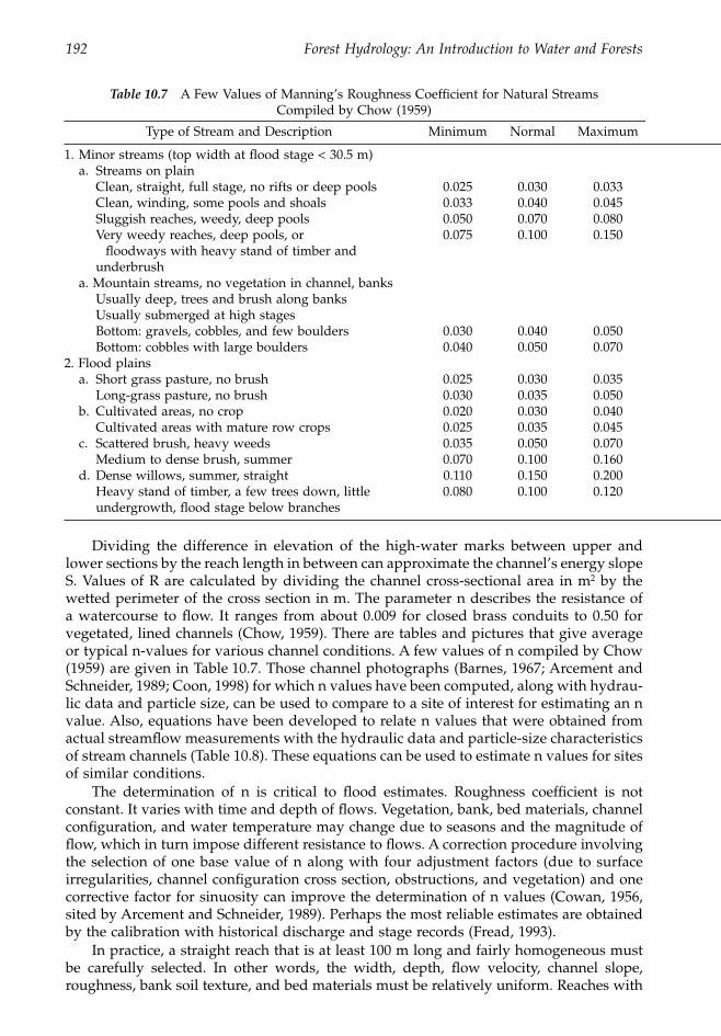
192 Forest Hydrology: An Introduction to Water and Forests
Dividing the difference in elevation of the high-water marks between upper andlower sections by the reach length in between can approximate the channel’s energy slopeS. Values of R are calculated by dividing the channel cross-sectional area in m2 by thewetted perimeter of the cross section in m. The parameter n describes the resistance ofa watercourse to flow. It ranges from about 0.009 for closed brass conduits to 0.50 forvegetated, lined channels (Chow, 1959). There are tables and pictures that give averageor typical n-values for various channel conditions. A few values of n compiled by Chow(1959) are given in Table 10.7. Those channel photographs (Barnes, 1967; Arcement andSchneider, 1989; Coon, 1998) for which n values have been computed, along with hydrau-lic data and particle size, can be used to compare to a site of interest for estimating an nvalue. Also, equations have been developed to relate n values that were obtained fromactual streamflow measurements with the hydraulic data and particle-size characteristicsof stream channels (Table 10.8). These equations can be used to estimate n values for sitesof similar conditions.
The determination of n is critical to flood estimates. Roughness coefficient is notconstant. It varies with time and depth of flows. Vegetation, bank, bed materials, channelconfiguration, and water temperature may change due to seasons and the magnitude offlow, which in turn impose different resistance to flows. A correction procedure involvingthe selection of one base value of n along with four adjustment factors (due to surfaceirregularities, channel configuration cross section, obstructions, and vegetation) and onecorrective factor for sinuosity can improve the determination of n values (Cowan, 1956,sited by Arcement and Schneider, 1989). Perhaps the most reliable estimates are obtainedby the calibration with historical discharge and stage records (Fread, 1993).
In practice, a straight reach that is at least 100 m long and fairly homogeneous mustbe carefully selected. In other words, the width, depth, flow velocity, channel slope,roughness, bank soil texture, and bed materials must be relatively uniform. Reaches with
Table 10.7 A Few Values of Manning’s Roughness Coefficient for Natural Streams Compiled by Chow (1959)
Type of Stream and Description Minimum Normal Maximum
1. Minor streams (top width at flood stage < 30.5 m)a. Streams on plain
Clean, straight, full stage, no rifts or deep pools 0.025 0.030 0.033Clean, winding, some pools and shoals 0.033 0.040 0.045Sluggish reaches, weedy, deep pools 0.050 0.070 0.080Very weedy reaches, deep pools, or 0.075 0.100 0.150 floodways with heavy stand of timber and underbrush
a. Mountain streams, no vegetation in channel, banksUsually deep, trees and brush along banksUsually submerged at high stagesBottom: gravels, cobbles, and few boulders 0.030 0.040 0.050Bottom: cobbles with large boulders 0.040 0.050 0.070
2. Flood plainsa. Short grass pasture, no brush 0.025 0.030 0.035
Long-grass pasture, no brush 0.030 0.035 0.050b. Cultivated areas, no crop 0.020 0.030 0.040
Cultivated areas with mature row crops 0.025 0.035 0.045c. Scattered brush, heavy weeds 0.035 0.050 0.070
Medium to dense brush, summer 0.070 0.100 0.160d. Dense willows, summer, straight 0.110 0.150 0.200
Heavy stand of timber, a few trees down, little undergrowth, flood stage below branches
0.080 0.100 0.120
1363_C10_fm Page 192 Wednesday, December 4, 2002 7:43 AM
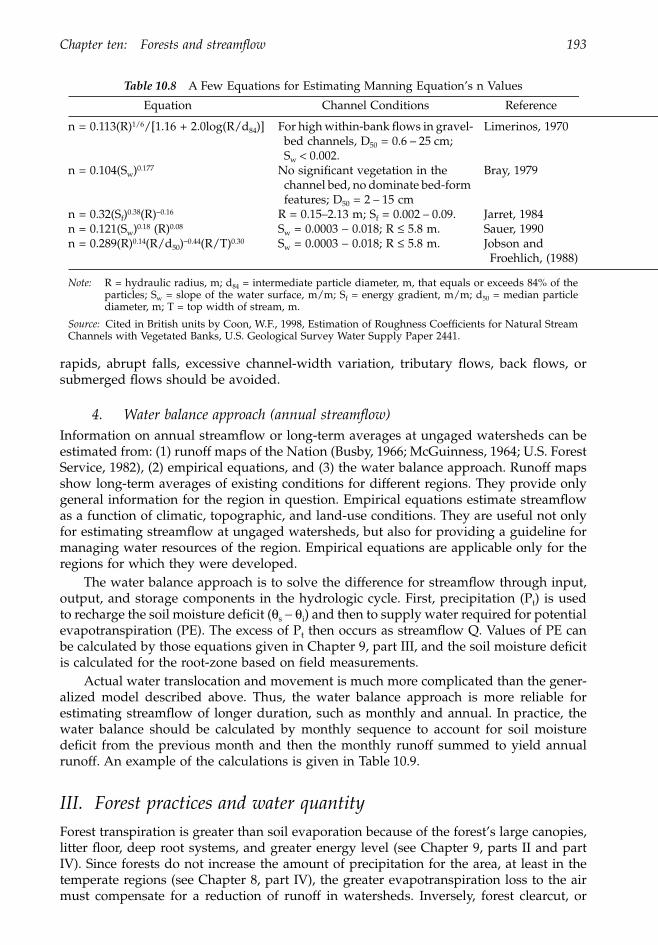
Chapter ten: Forests and streamflow 193
rapids, abrupt falls, excessive channel-width variation, tributary flows, back flows, orsubmerged flows should be avoided.
4. Water balance approach (annual streamflow)Information on annual streamflow or long-term averages at ungaged watersheds can beestimated from: (1) runoff maps of the Nation (Busby, 1966; McGuinness, 1964; U.S. ForestService, 1982), (2) empirical equations, and (3) the water balance approach. Runoff mapsshow long-term averages of existing conditions for different regions. They provide onlygeneral information for the region in question. Empirical equations estimate streamflowas a function of climatic, topographic, and land-use conditions. They are useful not onlyfor estimating streamflow at ungaged watersheds, but also for providing a guideline formanaging water resources of the region. Empirical equations are applicable only for theregions for which they were developed.
The water balance approach is to solve the difference for streamflow through input,output, and storage components in the hydrologic cycle. First, precipitation (Pt) is usedto recharge the soil moisture deficit (qs - qi) and then to supply water required for potentialevapotranspiration (PE). The excess of Pt then occurs as streamflow Q. Values of PE canbe calculated by those equations given in Chapter 9, part III, and the soil moisture deficitis calculated for the root-zone based on field measurements.
Actual water translocation and movement is much more complicated than the gener-alized model described above. Thus, the water balance approach is more reliable forestimating streamflow of longer duration, such as monthly and annual. In practice, thewater balance should be calculated by monthly sequence to account for soil moisturedeficit from the previous month and then the monthly runoff summed to yield annualrunoff. An example of the calculations is given in Table 10.9.
III. Forest practices and water quantityForest transpiration is greater than soil evaporation because of the forest’s large canopies,litter floor, deep root systems, and greater energy level (see Chapter 9, parts II and partIV). Since forests do not increase the amount of precipitation for the area, at least in thetemperate regions (see Chapter 8, part IV), the greater evapotranspiration loss to the airmust compensate for a reduction of runoff in watersheds. Inversely, forest clearcut, or
Table 10.8 A Few Equations for Estimating Manning Equation’s n Values
Equation Channel Conditions Reference
n = 0.113(R)1/6/[1.16 + 2.0log(R/d84)] For high within-bank flows in gravel-bed channels, D50 = 0.6 – 25 cm; Sw < 0.002.
Limerinos, 1970
n = 0.104(Sw)0.177 No significant vegetation in the channel bed, no dominate bed-form features; D50 = 2 – 15 cm
Bray, 1979
n = 0.32(Sf)0.38(R)-0.16 R = 0.15–2.13 m; Sf = 0.002 – 0.09. Jarret, 1984n = 0.121(Sw)0.18 (R)0.08 Sw = 0.0003 - 0.018; R £ 5.8 m. Sauer, 1990n = 0.289(R)0.14(R/d50)-0.44(R/T)0.30 Sw = 0.0003 - 0.018; R £ 5.8 m. Jobson and
Froehlich, (1988)
Note: R = hydraulic radius, m; d84 = intermediate particle diameter, m, that equals or exceeds 84% of theparticles; Sw = slope of the water surface, m/m; Sf = energy gradient, m/m; d50 = median particlediameter, m; T = top width of stream, m.
Source: Cited in British units by Coon, W.F., 1998, Estimation of Roughness Coefficients for Natural StreamChannels with Vegetated Banks, U.S. Geological Survey Water Supply Paper 2441.
1363_C10_fm Page 193 Wednesday, December 4, 2002 7:43 AM
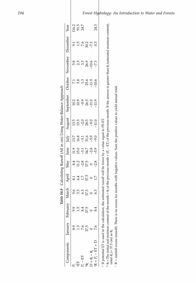
194 Forest Hydrology: An Introduction to Water and Forests
Tabl
e 10
.9C
alcu
lati
ng R
unof
f (A
ll in
cm
) U
sing
Wat
er-B
alan
ce A
ppro
ach
Com
pone
nts
Janu
ary
Febr
uary
Mar
chA
pril
May
June
July
Aug
ust
Sept
embe
rO
ctob
erN
ovem
ber
Dec
embe
rYe
ar
P t8.
99.
99.
68.
18.
411
.913
.713
.510
.27.
15.
89.
111
6.2
a ET
1.3
1.5
3.3
6.4
11.2
15.0
16.8
15.5
10.9
5.8
2.3
1.5
91.5
P t -
ET
7.6
8.4
6.3
1.7
-2.8
-3.1
-3.1
-2.0
-0.9
1.3
3.3
7.6
24.7
b q i37
.537
.537
.537
.537
.534
.731
.628
.526
.525
.626
.930
.2D
= q
i - q
s0
00
00
-2.8
-5.9
-9.0
-11.
0-1
1.9
-10.
6-7
.3c R
= P
t - E
T +
D7.
68.
46.
31.
7-2
.8-5
.9-9
.0-1
1.0
-11.
9-1
0.6
-7.3
0.3
24.3
aIf
pot
enti
al E
T is
use
d in
the
cal
cula
tion
, the
est
imat
ed r
unof
f w
ill b
e lo
wer
by
a va
lue
equa
l to
PE-E
T.b
q i =
The
init
ial s
oil m
oist
ure
cont
ent o
f the
mon
th =
qi o
f the
pre
viou
s m
onth
+ (P
t - E
T) o
f the
pre
viou
s m
onth
. If t
he a
nsw
er is
gre
ater
than
qs (s
atur
ated
moi
stur
e co
nten
t),
ente
r q s
(= 3
7.5
cm)
as q
i.c
R =
rai
nfal
l exc
ess
(run
off)
. The
re is
no
exce
ss f
or m
onth
s w
ith
nega
tive
val
ues.
Sum
the
pos
itiv
e va
lues
to
yiel
d a
nnua
l tot
al.
1363_C10_fm Page 194 Wednesday, December 4, 2002 7:43 AM
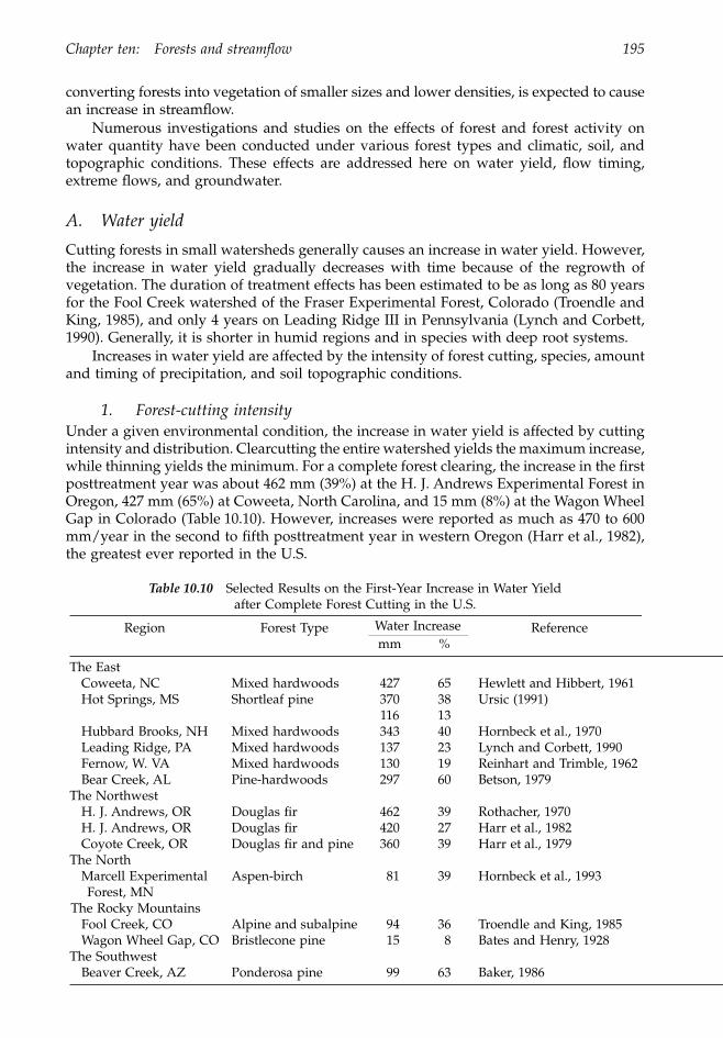
Chapter ten: Forests and streamflow 195
converting forests into vegetation of smaller sizes and lower densities, is expected to causean increase in streamflow.
Numerous investigations and studies on the effects of forest and forest activity onwater quantity have been conducted under various forest types and climatic, soil, andtopographic conditions. These effects are addressed here on water yield, flow timing,extreme flows, and groundwater.
A. Water yield
Cutting forests in small watersheds generally causes an increase in water yield. However,the increase in water yield gradually decreases with time because of the regrowth ofvegetation. The duration of treatment effects has been estimated to be as long as 80 yearsfor the Fool Creek watershed of the Fraser Experimental Forest, Colorado (Troendle andKing, 1985), and only 4 years on Leading Ridge III in Pennsylvania (Lynch and Corbett,1990). Generally, it is shorter in humid regions and in species with deep root systems.
Increases in water yield are affected by the intensity of forest cutting, species, amountand timing of precipitation, and soil topographic conditions.
1. Forest-cutting intensityUnder a given environmental condition, the increase in water yield is affected by cuttingintensity and distribution. Clearcutting the entire watershed yields the maximum increase,while thinning yields the minimum. For a complete forest clearing, the increase in the firstposttreatment year was about 462 mm (39%) at the H. J. Andrews Experimental Forest inOregon, 427 mm (65%) at Coweeta, North Carolina, and 15 mm (8%) at the Wagon WheelGap in Colorado (Table 10.10). However, increases were reported as much as 470 to 600mm/year in the second to fifth posttreatment year in western Oregon (Harr et al., 1982),the greatest ever reported in the U.S.
Table 10.10 Selected Results on the First-Year Increase in Water Yield after Complete Forest Cutting in the U.S.
Region Forest Type Water Increase Referencemm %
The EastCoweeta, NC Mixed hardwoods 427 65 Hewlett and Hibbert, 1961Hot Springs, MS Shortleaf pine 370 38 Ursic (1991)
116 13Hubbard Brooks, NH Mixed hardwoods 343 40 Hornbeck et al., 1970Leading Ridge, PA Mixed hardwoods 137 23 Lynch and Corbett, 1990Fernow, W. VA Mixed hardwoods 130 19 Reinhart and Trimble, 1962Bear Creek, AL Pine-hardwoods 297 60 Betson, 1979
The NorthwestH. J. Andrews, OR Douglas fir 462 39 Rothacher, 1970H. J. Andrews, OR Douglas fir 420 27 Harr et al., 1982Coyote Creek, OR Douglas fir and pine 360 39 Harr et al., 1979
The NorthMarcell Experimental Forest, MN
Aspen-birch 81 39 Hornbeck et al., 1993
The Rocky MountainsFool Creek, CO Alpine and subalpine 94 36 Troendle and King, 1985Wagon Wheel Gap, CO Bristlecone pine 15 8 Bates and Henry, 1928
The SouthwestBeaver Creek, AZ Ponderosa pine 99 63 Baker, 1986
1363_C10_fm Page 195 Wednesday, December 4, 2002 7:43 AM
196 Forest Hydrology: An Introduction to Water and Forests
These results provide evidence of forest removal as a potential for water yield aug-mentation. However, the augmentation of water yields in the U.S. is an attainable goalonly if: (1) forests cover a significant portion of the entire watershed (Douglass, 1983),(2) average precipitation exceeds 400 to 450 mm/year (Hibbert, 1983), and (3) forest coverreduction is greater than 20% (Stednick, 1996). Since most watershed studies were con-ducted in headwater areas, how much the downstream users can enjoy the upstreamincrease is an addressable question.
While there is great potential to augment water yield by 10 to 65% through forest cutting,it can impose adverse effects such as nutrient losses, soil erosion, lower water quality, andless aesthetic environments. Watershed managers select a less intensive cutting or a smallarea of clearcutting to mitigate the environmental problems that might be incurred by a large-scale harvesting (Gottfried, 1983; Johnston, 1984). Small openings in the watershed can alsobenefit timber and wildlife resources (Folliott and Thorud, 1977), are effective BMPs forcontrolling nonpoint sources of water pollution (Lynch and Corbett, 1990), and can improvestream habitats, consequently increasing the primary productivity of aquatic biota in head-water streams (Bureau of Land Management, 1987; Gregory et al., 1987).
The increase in water yield by partial cuttings is less than clearcutting, depending onintensity and distribution of the cutting. In the eastern U.S., increases in water yield forharvest of hardwoods can be estimated by the following equations (Douglass, 1983):
Y1 = 0.00224(BA/PI)1.4462 (10.30)
D = 1.5(Y1) (10.31)
Yi = Y1 + b log(i) (10.32)
where Y1 = the first year increase in inches for the harvest of hardwoods; BA = the percentbasal area cut of the watershed; PI = the annual potential insolation index, in 1 ¥ 10–6 calcm-2 for the watershed calculated by methods of Lee (1963) or Swift (1976); D = theduration of treatment effect in years; Yi = the yield increase in inches for the ith year aftertreatment; and b = coefficient derived by solving Equation 10.32 for the year when i = D,and Yi = 0.
For example, completely clearcutting an eastern hardwood watershed (BA = 100) inthe Appalachian Highland of West Virginia with the PI = 0.3 could increase water yieldin the first posttreatment year 9.97 in (25.3 cm). The increase would decline to 4.18 in.(10.6 cm) in the fifth year after treatment and to its pretreatment level in the 16th year. Ifthe watershed is cut by 50% of its basal area (BA = 50), then the first-year increase isreduced to 3.66 in. (9.3 cm), and it takes 6 years for water yield to return to its pretreatmentlevel.
In the West, a 67% selection cut in Caspar Creek dominated by redwood and Douglasfir in California caused an average annual increase in water yield of 94 mm or 15%(Keppeler and Ziemer, 1990). A 25% patch cut in Brownie Creek, Utah, dominated bylodgepole pine, increased annual streamflow by 147 mm or 52% (Burton, 1997). Cuttingby single-tree selection or thinning does not produce large increases in water yield (Tro-endle and King, 1987), unless the density is reduced to a basal area of 6.9 m2/ha as it wasin Beaver Creek, Arizona (Baker, 1986), or of 9.2 m2/ha as in Workman Creek, Arizona,(Rich and Gottfried, 1976).
Small openings in upper slopes can cause a smaller increase in water yield than thosein lower slopes or close to stream channels. Riparian vegetation and phreatophytes withroot systems extending into the groundwater table or capillary fringe transpire much more
1363_C10_fm Page 196 Wednesday, December 4, 2002 7:43 AM
Chapter ten: Forests and streamflow 197
water than mesophytes growing on uplands. Streamflow can be increased with relativelylittle work by eliminating riparian vegetation through mechanical eradication or transpi-ration suppression (Ingebo, 1971). However, the treatment of riparian vegetation is effec-tive only if: (1) the water supply exceeds ET loss after treatments, (2) the water table iswithin reach of the vegetation root systems, and (3) the soils are of sufficient depth topermit the reduction in ET if the deep-rooted vegetation is eliminated. Treatments needto be done with care due to possible soil erosion and water quality problems and incompliance with environmental regulations. However, riparian vegetation managementis more effective in the West than in the East (Lynch, 2001).
2. SpeciesPlant transpiration rate is different among species due to characteristic canopy, height,and root systems. Generally, conifers have greater total leaf-surface areas and retain foliageall year round; they intercept and transpire more water than hardwoods. Chaparrals aredeep-rooted evergreen shrubs with a large biomass above ground. Transpiration andinterception losses are greater for chaparrals than for grasses of shallower root systemsand longer dormancy period. The lower stem, smoother surface, and light-colored canopyof grasses cause the reflection of solar radiation to be greater, the energy absorption to belower, and consequently the water consumption to be less than those of woody plants. Inother words, deep-rooted evergreen species with large and dark canopies transpire a greatdeal more water every year than shallow-rooted deciduous species with small and light-colored canopies. Thus, transpiration rate in general is greatest for conifers, followed byhardwoods, chaparrals, and grasses. Converting species composition in watersheds fromhigher transpiration rate to lower transpiration rate increases water yield.
Many watershed observations have provided evidence on increases in water yieldthrough manipulation of species composition (Table 10.11). In the West, water yields wereincreased up to 150 mm/year by converting chaparrals into grasses. However, the speciesconversion is effective only if it is conducted in areas where: (1) the soil depth is morethan 1.0 m, (2) precipitation is greater than 400 mm/year, (3) annual ET is less than annualprecipitation, and (4) the introduced grasses are shallow-rooted species.
A pioneer government project has been initiated to augment water supply throughbrush control in Texas. There, about 130 million mesquites and 100 million junipers robwest Texas of almost 2.5 km3 of water every year. In 1985, Texas Senate Bill 1083 createdthe Texas Brush Control Program, which is administered by the Texas State Soil and WaterConservation Board through local soil and water conservation districts, to prepare andadopt a state brush-control plan. A brush-control feasibility study was conducted on theNorth Concho Watershed at Carsbad in 1997. The results showed that as much as4132 m-ha of water could be saved per year, or about five times the current flow. In 1999,the House Bill 1592 funded a 2-year, $7 million pilot program for brush-control cost sharein the North Concho River Watershed. The success of the brush-control project will providean attractive approach to mitigating water stress in the West.
3. PrecipitationForest manipulation for water augmentation is more effective in humid regions and duringwet years. Also, precipitation enhances rapid growth of vegetation, and the duration oftreatment effects in humid regions is shorter than that in arid regions. In the chaparralcountry of California and Arizona, precipitation is the major factor in water-yield responseto species conversion. In areas where average annual precipitation is less than 400 mm,there is no potential for increasing water; and for areas with precipitation between 400and 500 m, the increase is likely to be marginal. On western rangelands of the U.S., the
1363_C10_fm Page 197 Wednesday, December 4, 2002 7:43 AM
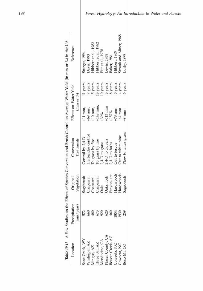
198 Forest Hydrology: An Introduction to Water and Forests
Tabl
e 10
.11
A F
ew S
tud
ies
on t
he E
ffec
ts o
f Sp
ecie
s C
onve
rsio
n an
d B
rush
Con
trol
on
Ave
rage
Wat
er Y
ield
(in
mm
or
%)
in t
he U
.S.
Loc
atio
nPr
ecip
itat
ion
(m
m/
year
)O
rigi
nal
Veg
etat
ion
Con
vers
ion
Tr
eatm
ents
Eff
ects
on
Wat
er Y
ield
(m
m o
r %
)R
efer
ence
Sane
Cre
ek, W
Y57
2Sa
gebr
ush
Con
trol
by
2,4-
D+
11 m
m,
11 y
ears
Stur
ges,
199
4W
hite
spar
, AZ
660
Cha
parr
alH
erbi
cid
es c
ontr
ol+
69 m
m,
7 ye
ars
Dav
is, 1
993
Min
gus,
AZ
480
Cha
parr
alTo
gra
ss b
y fir
e+
10 m
m,
5 ye
ars
Hib
bert
et a
l., 1
982
Thr
ee B
ar, A
Z67
3C
hapa
rral
To g
rass
by
fire
+14
8 m
m,
18 y
ears
Hib
bert
et a
l., 1
982
Men
doc
ino,
CA
920
Oak
s2,
4-D
to
gras
s+
39%
10 y
ears
Pitt
et a
l., 1
978
Plac
er C
ount
y, C
A62
0O
aks,
for
b2,
4-D
to
clov
ers
+11
3 m
m3
year
sL
ewis
, 196
8B
eave
r C
reek
, AZ
460
Piny
on, e
tc.
2,4-
D t
o fo
rbs
+15
7%8
year
sB
aker
, 198
4C
owee
ta, N
C18
54H
ard
woo
ds
Cut
to
fesc
ue+
78 m
m5
year
sH
ibbe
rt, 1
969
Cow
eeta
, NC
1930
Har
dw
ood
sC
ut t
o w
hite
pin
e-6
4 m
m4
year
sSw
ank
and
Min
er, 1
968
Boc
o M
t, C
O25
9Sa
gebr
ush
Plow
to
whe
atgr
ass
-9 m
m6
year
sL
usby
, 197
9
1363_C10_fm Page 198 Wednesday, December 4, 2002 7:43 AM
Chapter ten: Forests and streamflow 199
mean annual increase in water yield Q in mm was related to mean annual precipitationP in mm by (Hibbert, 1983):
Q = –100 + 0.26 (Pt) (10.33)
in which Pt has to be >385 mm/year for any positive forest treatment effects on Q. Atthe H.J. Andrews Experimental Forest in western Oregon, Harr (1983) showed thatincreases in water yield due to harvest of Douglas-fir forest in watershed HJA-1 couldbe estimated by:
Qi = 308 + 0.87(Pt) – 18.1 (Yi) (10.34)
where Qi = the predicted annual increase of water in mm in ith year after harvest, Pt =annual precipitation in mm, and Yi = the ith year after harvesting.
Equations 10.33 and 10.34 show that the precipitation effect on yield increase is muchgreater in the Northwest than in the Southwest of the U.S. Water yield increases about 1mm for each 1 mm increase in precipitation at watershed HJA-1 and for each 4 mm increasein precipitation in the Southwest. This difference is probably associated with: (1) climaticfactors such as temperature and monthly distribution of precipitation, (2) soil topographicfactors such as soil depth and the gradient, aspect, shape of slopes, and (3) vegetal factorssuch as species, age, and treatments.
4. Soil topographic conditionsHydrological responses to forest harvests vary among watersheds due to the type anddepth of soils along with steepness and orientation of the watershed. Soils of deep andfine textures have a much greater water-holding capacity than soils of shallow and coarsetextures, consequently a greater potential for yield increase. Rowe and Reimann (1961)stated that water yield could not be appreciably increased in soils with depth less thanabout 1 m.
Slope aspect affects solar radiation, precipitation, and wind speed, consequently soiland air temperatures, snow accumulation, snowmelt, ET, and vegetation type and growth.Forest transpiration is generally greater in northern than in southern slopes because ofdenser vegetative cover and deeper soils (Bethlahmy, 1973). Actual observations showedthat clearcutting on south-facing slopes caused only about a one-third increase of thatmeasured on north-facing slopes in Idaho (Cline et al., 1977) and at Coweeta, NorthCarolina (Douglass, 1983).
B. Timing of streamflow
The seasonal distribution of water yield associated with forest management is not uniformthroughout the year. Since increases in water yield caused by forest cutting are attributableto the reduction in canopy interception and transpiration, a large proportion of increasedflow must occur during the growing season. However, superimposed on this vegetal effectare precipitation type and seasonal distribution.
In areas where precipitation is dominated by rainfall with no significant distributionpattern throughout the year, such as the eastern U.S., most of the flow increases occur insummer and fall. The impact of forest cutting on water yield in winter and early springis insignificant when both cut and uncut watersheds are saturated and ET is minimum.For an eastern hardwood forest that was cut annually during a 7-year period, Swank andJohnson (1994) showed that 76% of the mean monthly increase in runoff occurred duringthe low-flow period, July to December.
1363_C10_fm Page 199 Wednesday, December 4, 2002 7:43 AM
200 Forest Hydrology: An Introduction to Water and Forests
In the Rocky Mountain region, where precipitation is dominated by snow and 70 to80% of the total annual runoff occurs during the summer months, forest clearing reducesET and enhances snow accumulation and snowmelt. Thus, the greatest increase in wateryield occurs during the snowmelt period. The classic study on the Fool Creek Watershed inColorado showed that increases in runoff were primarily on the rising side of the annualhydrograph with May being the greatest, accounting for more than 50% of the estimatedannual increase (Troendle, 1983). However, a 25% harvest of lodgepole-pine forest on a largewatershed (2145 ha) in northeastern Utah gave a different perspective. The cutting causedan average increase in runoff of 52% (14.7 cm) per year, but increases occurred primarily onthe recession limb of the annual hydrograph (May through August) with little or no changein winter (Burton, 1997). Hydrologic storage is greater in large watersheds, which can haveimplications for its timing on flow increases different from small watersheds.
In areas where summer is dry and the majority of precipitation occurs in fall andwinter, the greatest proportion of water-yield increase due to forest cutting occurs duringthe rainy season. For example, about 80% of annual precipitation in western Washingtonand Oregon occur between October and March, and major increases occur between Decem-ber and March when there is plenty of streamflow and no agricultural demand for water.Although large in relative terms, summer increases are small in absolute value when waterstress is high. Thus, without storage facilities, water increases in winter seem to be of littleeconomic benefit downstream when water is most needed (Harr et al., 1979).
C. Flow extremes
For quite some time, forests have been speculatively claimed as streamflow moderatorsby making high flows lower and low flows higher. Numerous watershed observationsand studies in the last century have provided many new perspectives on the speculationof forest–water relationships. If forest clearings do increase water yield in watersheds, asdiscussed in the previous sections, then the increase must be attributable to quick flows,low flows, or both. Timber harvests have been shown to cause low flows higher inmagnitude, shorter in duration, and less frequent in occurrence (Troendle, 1970; Harr et al.,1982; Swank and Vose, 1994). However, the effect on quick (storm) flows is highly variable.It can be an increase (Burton, 1997), no change (Hewlett and Hibbert, 1961), and even adecrease (Harr and McCorison, 1979), depending on the severity of soil disturbance,cutting intensity and distribution, size and distribution of storms, antecedent soil-moisturecondition, and precipitation type.
1. Peak flowsFor a given region, peak flows are generally lower in watersheds with a greater percentageof forested area (Reich, 1972; Chang and Waters, 1984). Thus, cutting forests can cause anincrease in peak flows. Reported increases include 15% at Coweeta, North Carolina (Swankand Johnson, 1994), 35–122% in coastal Oregon (Harr, 1976), 10–89% in the Horse CreekWatersheds, Idaho (King, 1989), 66% in Brownie Creek, Utah (Burton, 1997), 180% in UpperBear Creek, Alabama (Betson, 1979) and 340 to 880% on Leading Ridge-2, Pennsylvania(Lynch and Corbett, unpublished report). The causes can be attributable to more saturatedsoils, soil compaction, road construction, and differences in snow accumulation and snow-melt. However, peak flows can also be decreased or remain unchanged after logging(Thomas and Megahan, 1998), depending on cutting intensity, location in the watershed,regrowth of vegetation, and climatic patterns. As long as the forest floor remains intact,the effect of clearcutting on peak flows could be significantly reduced (Harr et al., 1979).
The increase in peak flows occurred generally in the growing season, and quick flowswere a small portion of the total water increases. For example, of the average increase
1363_C10_fm Page 200 Wednesday, December 4, 2002 7:43 AM
Chapter ten: Forests and streamflow 201
of 280 mm/year in the Hubbard Brook Experimental Forest, New Hampshire, only 99mm or 35.4% occurred as quick flows (Hornbeck et al., 1970). In other words, most ofthe streamflow increase was in the form of base flow. Storm-runoff events occurring afterfall recharge of soil moisture and before the start of spring snowmelt were unchangedby clearing. This is a desirable effect because streamflow increase in the form of baseflow is of more value than quick flow. Also, the occurrence of peak flows in the growingseason poses little danger than if the peak flows occur during the seasons when stream-flow is high.
Although low peak flows occur in forested watersheds and high peak flows resultfrom forest cutting, it is not necessary to imply that forests can be relied on for floodingprevention. It is true that forests, due to the great amount of transpiration loss and theincrease in soil water-holding capacity, are the most effective types of vegetation in reduc-ing streamflow. Flood damage in forested areas is also the smallest among all naturalsurface conditions due to forests’ control on soil erosion, landslide, and channel stability.However, when the soil is saturated, any additional rainfalls will run off from the water-shed whether it is forested or nonforested. Thus, forests can reduce peak flows for stormsof short duration and low intensity, but cannot prevent the occurrence of floods that areproduced from storms of high intensity and long duration over a large area.
2. Low flowsThe increase in water yield due to timber harvest results basically from increases at lowflow levels, especially during the growing season. This has been reported in many regionsincluding Minnesota (Verry, 1972), New Hampshire (Hornbeck, 1973), New York (Satter-lund and Eschner, 1965), North Carolina (Swank and Vose, 1994), Pennsylvania (Lynchet al., 1980), western Oregon (Harr et al., 1982), and West Virginia (Patric and Reinhart,1971). For example, timber harvest resulted in fewer low-flow days in both clearcut andshelterwood cut watersheds in the H.J. Andrews Experimental Forest, Oregon. In 1977,by far the driest year on record in western Oregon, the clearcut watershed had only 8 low-flow days instead of 143 days predicted by the prelogging relationship. For the shelter-wood watershed, it had only 2 low-flow days instead of 135 days predicted by thecalibration equation (Harr et al., 1982).
3. Flow durationFlow duration is often depicted by flow-duration curves. A flow-duration curve is acumulative curve of the percentage time that a given flow magnitude is equaled orexceeded. Thus, the percent time of occurrence is greater for flows of lower magnitudethan for flows of higher magnitude.
In West Virginia, forest harvest increased the magnitude of both high and low flowsfor all frequencies of occurrence (Figure 10.9). Low flows were substantially augmentedin both the wet and the dry year (Reinhart et al., 1963). Conversely, the frequency of bothhigh and low flows was significantly reduced when two watersheds were converted fromeastern hardwoods to white-pine plantation in Coweeta, North Carolina (Swank and Vose,1994). By age 24 on one of the watersheds, high flows at 1 and 5% of time were reducedby 33 and 52%, respectively. Flows for other percentage of time were reduced 37 to 60%below predicted values (Figure 10.9).
Forty percent of the aforementioned Fool Creek Watershed (290 ha) on the FraserExperimental Forest, Colorado, was strip clearcut during 1954–1956. Total seasonal flow(1956–1971) increased 40%, peakflow increased 20%, and most detectable changes occurredin May. The increases appeared to be most for the flow durations in the range from 80 to120% of bankfull; the highest flow durations were not affected (Troendle and Olsen, 1993).
1363_C10_fm Page 201 Wednesday, December 4, 2002 7:43 AM
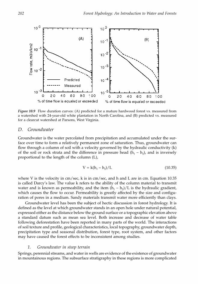
202 Forest Hydrology: An Introduction to Water and Forests
D. Groundwater
Groundwater is the water percolated from precipitation and accumulated under the sur-face over time to form a relatively permanent zone of saturation. Thus, groundwater canflow through a column of soil with a velocity governed by the hydraulic conductivity (k)of the soil or rock strata and the difference in pressure head (h1 - h2), and is inverselyproportional to the length of the column (L),
V = k(h1 – h2)/L (10.35)
where V is the velocity in cm/sec, k is in cm/sec, and h and L are in cm. Equation 10.35is called Darcy’s law. The value k refers to the ability of the column material to transmitwater and is known as permeability, and the item (h1 - h2)/L is the hydraulic gradient,which causes the flow to occur. Permeability is greatly affected by the size and configu-ration of pores in a medium. Sandy materials transmit water more efficiently than clays.
Groundwater level has been the subject of hectic discussion in forest hydrology. It isdefined as the level at which groundwater stands in an open hole under natural potential,expressed either as the distance below the ground surface or a topographic elevation abovea standard datum such as mean sea level. Both increase and decrease of water tablefollowing deforestation have been reported in many parts of the world. The interactionsof soil texture and profile, geological characteristics, local topography, groundwater depth,precipitation type and seasonal distribution, forest type, root system, and other factorsmay have caused the forest effects to be inconsistent among studies.
1. Groundwater in steep terrainSprings, perennial streams, and water in wells are evidence of the existence of groundwaterin mountainous regions. The subsurface stratigraphy in these regions is more complicated
Figure 10.9 Flow duration curves: (A) predicted for a mature hardwood forest vs. measured froma watershed with 24-year-old white plantation in North Carolina, and (B) predicted vs. measuredfor a clearcut watershed at Parsons, West Virginia.
1363_C10_fm Page 202 Wednesday, December 4, 2002 7:43 AM
Chapter ten: Forests and streamflow 203
than that of level terrain, which can create a perched groundwater table (isolated zone ofsaturation) in the soil profile or disrupt the groundwater table. Groundwater in these areascan also be deep under the ground. The ability of forests in these areas to sustain springsand streamflow — and the disappearance of springs after deforestation — have beenreported (Zon, 1927; Molchanov, 1963; Pritchett, 1979). On the other hand, increases ingroundwater following deforestation have also been cited in many reports (Hamilton andKing, 1983). A higher groundwater table under forests than in the open may reflect specificsite conditions optimal for infiltration of precipitation. In steep topography, open areasmay have greater evaporation and runoff, reducing water entering the ground.
In areas where groundwater is shallow, the most immediate effect of forests is theaccess of their root systems to the water table. Here groundwater is subject to diurnal andseasonal fluctuations in response to transpiration losses (Groeneveld and Or, 1994). Thediurnal pattern of fluctuations is most distinct near small headwater streams; it can beused as an estimate of evapotranspiration rate over time. In areas where soils are frozenand precipitation is dominated by snow, forests can increase snow accumulation and delaysnowmelt in the spring. This frequently results in an increase of precipitation infiltrationand consequently raises the groundwater table to above those groundwater tables in theopen (Pereira, 1973).
2. Groundwater in level terrainIn areas of gently level terrain where the subsurface conditions are more uniform and thehorizontal movement of groundwater is slow, forests lower the groundwater table. Theforest–groundwater relation is consistent in many studies including those in South Africa(Wicht, 1949), Italy (Wilde at al., 1953), Denmark (Holstener-Jorgensen, 1967), Finland(Heikurainen, 1967), the U.S. (Urie, 1977; Williams and Lipscomb, 1981; Riekerk, 1989),Australia (Borg et al., 1988), and others. Those studies showed that the fluctuations ingroundwater tables reflected the differences in transpiration rate caused by seasons, timeof the day, hardwoods vs. conifers, clearcutting intensities, and land-use conditions.
In low-lying swampy areas where groundwater is excessive, lowering the groundwa-ter table by forest transpiration can be beneficial to economic use of the site. However,water-loving plants and trees (phreatophytes) along streams and canals can be detrimentalto water supply in arid and semiarid areas. While clearing phreatophytes is an approachto conserving water resources in arid areas, cutting forests in humid low-lying areas suchas the southeast Coastal Plains can bring groundwater to the surface horizons. It thenturns the whole area into a water-logged site, creating an anaerobic condition that isharmful to root development, retardatory to tree growth, and very detrimental to forestregeneration.
For example, more than 120,000 ha of somewhat poorly drained saline soils supportmature loblolly (P. taeda) and shortleaf (P. echinata) pines in central east Texas. Artificialpine regeneration on the clearcut sites of these soils is extremely difficult, with failure inthree attempts in some cases. Transpiration and interception reduction raises the ground-water level, which may have brought salt along with it to near the surface. Thus, seedlingmortality may have been caused by high water tables, toxic salt concentrations, nutrientimbalance, or combinations of all three (Chang et al., 1994).
In western Australia, completely converting a forested watershed into agriculturemoved the groundwater table upward more than 2.7 m/year in a 4-year period. Thiswas equivalent to an increase in recharge of 6 to 12% of rainfall (Peck and Williamson,1987). Wilde et al. (1953) referred to the experience of Trappist monks at the Fontana,near Rome, Italy, on malarial swamplands. Planting a deep-rooted, fast growing speciesof eucalyptus lowered the groundwater table 1 m and greatly reduced the mosquitopopulation.
1363_C10_fm Page 203 Wednesday, December 4, 2002 7:43 AM
204 Forest Hydrology: An Introduction to Water and Forests
IV. Forest practices and water qualityForested watersheds are generally at high elevations and in remote areas with littledevelopment and few disturbances. Forest canopies, floor, and root systems also providethe best mechanisms in nature to protect the watershed from accelerated soil erosion,landslides, and nutrient losses. Coupling these conditions with cooler water temperatures,due either to higher elevation or the shading effect of riparian vegetation, makes thequality of water flowing through forested watersheds better than in other surface condi-tions (Table 10.12).
Since forests are subject to use and management for their various resources, activitiesin forested areas can destroy the equilibrium of the ecosystem and adversely affect waterquality. However, with proper operational techniques and management, the adverseeffects can be reduced to insignificant levels.
A. Water-quality determination
Stream water quality refers to the levels of the physical, chemical, and biological propertiesof water that can affect aquatic environments and intended water usage. These propertiesare induced by the concentrations of various substances dissolved in the water and theirinteractions with the natural environment. The concentration levels of those constituentsare minimal and stable when the water–soil–vegetation–atmosphere system within thewatershed is in equilibrium. However, the levels can be greatly altered and water qualitysignificantly impaired when human activities or natural actions disturb the watershedequilibrium. The degradation of water quality caused by human activities is often referredto as water pollution.
Water pollutants are generally grouped into categories such as sediment, plant nutrients,heat, oxygen-demanding wastes, inorganic chemicals and minerals, disease-causing agents,synthetic compounds, and radioactive substances (Chapter 6, part IV). Sediment. whichconsidered by far the nation’s largest single water pollutant, is discussed in great detail inChapter 11. This section is more concerned with water chemistry and other pollutants.
1. Input–output budgetsElements in a stream are the output components in the watershed chemical budget system.Elements can be deposited to the watershed with precipitation, released from soils throughweathering processes, mineralized from organic matter by biological activity, and leached
Table 10.12 Mean Concentrations and Yields of Total Nitrogen (N) and Total Phosphorous (P) under Various Cover Conditions in the U.S.
Land Cover Concentration (mg/l) Yield (kg/ha/year)Total N Total P Total N Total P
≥90% forest 0.598 0.018 3.47 0.091≥75% forest 0.643 0.024 3.54 0.129≥75% rangeland 1.297 0.097 1.04 0.065≥40% urban 1.818 0.092 7.30 0.347≥75% agriculture 2.702 0.140 5.55 0.255≥90% agriculture 5.354 0.161 9.54 0.266
Source: Omernik, J.M., 1976, Nonpoint Source–Stream Nutrient Level Relationships: A Nationwide Study, EPA-600/3–77–105, EPA Environ. Res. Lab., Corvallis, OR.
1363_C10_fm Page 204 Wednesday, December 4, 2002 7:43 AM
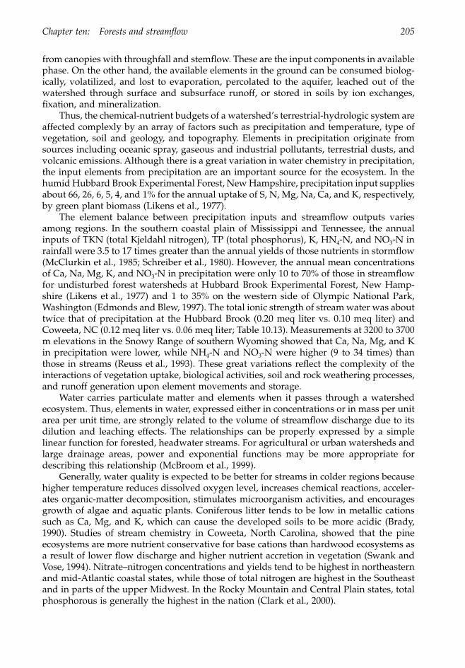
Chapter ten: Forests and streamflow 205
from canopies with throughfall and stemflow. These are the input components in availablephase. On the other hand, the available elements in the ground can be consumed biolog-ically, volatilized, and lost to evaporation, percolated to the aquifer, leached out of thewatershed through surface and subsurface runoff, or stored in soils by ion exchanges,fixation, and mineralization.
Thus, the chemical-nutrient budgets of a watershed’s terrestrial-hydrologic system areaffected complexly by an array of factors such as precipitation and temperature, type ofvegetation, soil and geology, and topography. Elements in precipitation originate fromsources including oceanic spray, gaseous and industrial pollutants, terrestrial dusts, andvolcanic emissions. Although there is a great variation in water chemistry in precipitation,the input elements from precipitation are an important source for the ecosystem. In thehumid Hubbard Brook Experimental Forest, New Hampshire, precipitation input suppliesabout 66, 26, 6, 5, 4, and 1% for the annual uptake of S, N, Mg, Na, Ca, and K, respectively,by green plant biomass (Likens et al., 1977).
The element balance between precipitation inputs and streamflow outputs variesamong regions. In the southern coastal plain of Mississippi and Tennessee, the annualinputs of TKN (total Kjeldahl nitrogen), TP (total phosphorus), K, HN4-N, and NO3-N inrainfall were 3.5 to 17 times greater than the annual yields of those nutrients in stormflow(McClurkin et al., 1985; Schreiber et al., 1980). However, the annual mean concentrationsof Ca, Na, Mg, K, and NO3-N in precipitation were only 10 to 70% of those in streamflowfor undisturbed forest watersheds at Hubbard Brook Experimental Forest, New Hamp-shire (Likens et al., 1977) and 1 to 35% on the western side of Olympic National Park,Washington (Edmonds and Blew, 1997). The total ionic strength of stream water was abouttwice that of precipitation at the Hubbard Brook (0.20 meq liter vs. 0.10 meq liter) andCoweeta, NC (0.12 meq liter vs. 0.06 meq liter; Table 10.13). Measurements at 3200 to 3700m elevations in the Snowy Range of southern Wyoming showed that Ca, Na, Mg, and Kin precipitation were lower, while NH4-N and NO3-N were higher (9 to 34 times) thanthose in streams (Reuss et al., 1993). These great variations reflect the complexity of theinteractions of vegetation uptake, biological activities, soil and rock weathering processes,and runoff generation upon element movements and storage.
Water carries particulate matter and elements when it passes through a watershedecosystem. Thus, elements in water, expressed either in concentrations or in mass per unitarea per unit time, are strongly related to the volume of streamflow discharge due to itsdilution and leaching effects. The relationships can be properly expressed by a simplelinear function for forested, headwater streams. For agricultural or urban watersheds andlarge drainage areas, power and exponential functions may be more appropriate fordescribing this relationship (McBroom et al., 1999).
Generally, water quality is expected to be better for streams in colder regions becausehigher temperature reduces dissolved oxygen level, increases chemical reactions, acceler-ates organic-matter decomposition, stimulates microorganism activities, and encouragesgrowth of algae and aquatic plants. Coniferous litter tends to be low in metallic cationssuch as Ca, Mg, and K, which can cause the developed soils to be more acidic (Brady,1990). Studies of stream chemistry in Coweeta, North Carolina, showed that the pineecosystems are more nutrient conservative for base cations than hardwood ecosystems asa result of lower flow discharge and higher nutrient accretion in vegetation (Swank andVose, 1994). Nitrate–nitrogen concentrations and yields tend to be highest in northeasternand mid-Atlantic coastal states, while those of total nitrogen are highest in the Southeastand in parts of the upper Midwest. In the Rocky Mountain and Central Plain states, totalphosphorous is generally the highest in the nation (Clark et al., 2000).
1363_C10_fm Page 205 Wednesday, December 4, 2002 7:43 AM
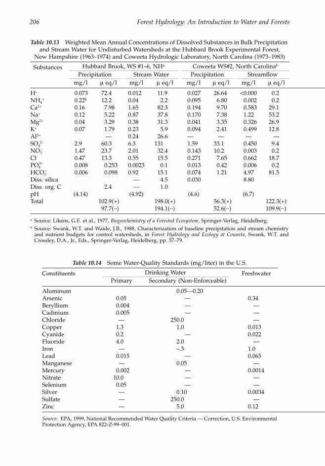
206 Forest Hydrology: An Introduction to Water and Forests
Table 10.13 Weighted Mean Annual Concentrations of Dissolved Substances in Bulk Precipitation and Stream Water for Undisturbed Watersheds at the Hubbard Brook Experimental Forest,
New Hampshire (1963–1974) and Coweeta Hydrologic Laboratory, North Carolina (1973–1983)
Substances Hubbard Brook, WS #1–6, NHa Coweeta WS#2, North Carolinab
Precipitation Stream Water Precipitation Streamflowmg/l m eq/l mg/l m eq/l mg/l m eq/l mg/l m eq/l
H+ 0.073 72.4 0.012 11.9 0.027 26.64 <0.000 0.2NH4
+ 0.22b 12.2 0.04 2.2 0.095 6.80 0.002 0.2Ca2+ 0.16 7.98 1.65 82.3 0.194 9.70 0.583 29.1Na+ 0.12 5.22 0.87 37.8 0.170 7.38 1.22 53.2Mg2+ 0.04 3.29 0.38 31.3 0.041 3.35 0.326 26.9K+ 0.07 1.79 0.23 5.9 0.094 2.41 0.499 12.8Al3+ — 0.24 26.6 — — — —SO4
2- 2.9 60.3 6.3 131 1.59 33.1 0.450 9.4NO3
– 1.47 23.7 2.01 32.4 0.143 10.2 0.003 0.2Cl- 0.47 13.3 0.55 15.5 0.271 7.65 0.662 18.7PO4
3- 0.008 0.253 0.0023 0.1 0.013 0.42 0.006 0.2HCO3
- 0.006 0.098 0.92 15.1 0.074 1.21 4.97 81.5Diss. silica — 4.5 0.030 8.80Diss. org. C 2.4 — 1.0pH (4.14) (4.92) (4.6) (6.7)Total 102.9(+) 198.0(+) 56.3(+) 122.3(+)
97.7(-) 194.1(-) 52.6(-) 109.9(-)
a Source: Likens, G.E. et al., 1977, Biogeochemistry of a Forested Ecosystem, Springer-Verlag, Heidelberg.b Source: Swank, W.T. and Waide, J.B., 1988, Characterization of baseline precipitation and stream chemistry
and nutrient budgets for control watersheds, in Forest Hydrology and Ecology at Coweeta, Swank, W.T. andCrossley, D.A., Jr., Eds., Springer-Verlag, Heidelberg, pp. 57–79.
Table 10.14 Some Water-Quality Standards (mg/liter) in the U.S.
Constituents Drinking Water FreshwaterPrimary Secondary (Non-Enforceable)
Aluminum 0.05—0.20Arsenic 0.05 — 0.34Beryllium 0.004 — —Cadmium 0.005 — —Chloride — 250.0 —Copper 1.3 1.0 0.013Cyanide 0.2 — 0.022Fluoride 4.0 2.0 —Iron — –.3 1.0Lead 0.015 — 0.065Manganese — 0.05 —Mercury 0.002 — 0.0014Nitrate 10.0 — —Selenium 0.05 — —Silver — 0.10 0.0034Sulfate — 250.0 —Zinc — 5.0 0.12
Source: EPA, 1999, National Recommended Water Quality Criteria — Correction, U.S. EnvironmentalProtection Agency, EPA 822-Z-99–001.
1363_C10_fm Page 206 Wednesday, December 4, 2002 7:43 AM
Chapter ten: Forests and streamflow 207
2. Water-quality criteriaSubstances dissolved in water can alter the physical, chemical, and biological propertiesof the water and limit its suitability for usage. Established by state and federal governments,water-quality criteria are a management approach designed to regulate the discharge ofpollutants into receiving streams and to provide desirable requirements for the intendeduse of the water. They are based on research and long-term observations on the acute andchronic effects of each pollutant. Thus, a quality standard may need to be modified whennew evidence on tolerant levels is substantial and significant.
The Clean Water Act identifies water uses into five categories: (1) public water supply,(2) recreation and aesthetic value, (3) aquatic life, (4) agriculture, and (5) industries. Eachrequires a set of water-quality criteria different from the others’. Generally, the criteriathat require large volume are not as rigid as those require smaller volume. Water-qualitycriteria for recreation and aquatic life should consider local variations due to differencesin climatic, soil, and geological conditions. For example, the minimum level for dissolvedoxygen in warm, slow-moving streams in the South should be lower than in the cold, fast-moving streams in the Northwest. Even in the same state, standards for surface watermay be different among watersheds (TNRCC, 1995). The EPA’s drinking-water and sur-face-water standards for a few constituents are given in Table 10.14.
B. Forest practices
Forested watersheds normally yield streamflow with better quality than that from otherland uses (Chang et al., 1983). The average total nitrogen concentration in forested streamswas about 0.850 mg/liter in the U.S. compared with 4.170 mg/liter for agricultural lands.For total phosphorous concentrations, it was 0.014 mg/liter for forested lands and 0.135mg/liter for agricultural lands (Omernik, 1976). Specific conductance is a parameter tomeasure the ability of water to conduct electric currents and is dependent upon the totalquantity of dissolved ions. It ranges from 3 to 15 mS/m in forested watersheds (Binkleyand Brown, 1993), and from 276 to 3855 mS/m for the Lower Arkansas River, an agricul-tural drainage basin in the Central Plain (Lewis and Brendle, 1998).
The higher water quality in forested watersheds is attributable to: (1) more uptake ofnutrients and ions by plants, (2) fewer runoff and sediment losses, (3) lower rates oforganic-matter decomposition and microbial activity, (4) cooler temperature, and (5) lessmanagement. Forest-management practices often remove vegetation, expose the groundto direct environmental impacts, and disturb soils. As a result, the forest functions men-tioned above are largely reduced and water quality is impaired.
1. ClearcuttingClearcutting — felling and removing essentially all trees from a forest — intends to createa site and microclimate for generation of an even-aged forest. It has been the majorapproach of the silvicultural systems in North America because of its efficiency in woodproduction and low costs (Kellogg et al., 1996). Since the method is the most intensiveamong forest-harvesting practices, its potential for causing adverse effects on stream waterquality is also the greatest.
Besides stream sediment, clearcutting can adversely affect stream temperature, con-centrations of water chemicals, dissolved oxygen, biochemical oxygen demand, specificconductance, pH, fecal coliform and fecal streptococcus, and aquatic environment (Eschnerand Larmoyeux, 1963; Binkley and Brown, 1993; Bolstad and Swank, 1997). However,these effects are highly variable, depending on the clearcutting system, species, soils andtopography, and climate. A tractor harvest system can create 35% bare soil and 26%
1363_C10_fm Page 207 Wednesday, December 4, 2002 7:43 AM
208 Forest Hydrology: An Introduction to Water and Forests
compacted soil, while a highlead harvest system can only create 15 and 9%, in that order(Adams, 1999).
For example, clearcutting northern hardwoods in New Hampshire caused increasesin NO3
– over 50-fold (averaged 15 mg/liter) and Al+3 by almost 10-fold, and decreases inpH by 0.3 units (Likens et al., 1977). In contrast, clearcuttings caused measurable increasesin concentrations of NO3
– (0.015 to 0.7 mg/liter), K+, and other constituents in northwesternNorth Carolina, but the magnitude of changes was small and unimportant to downstreamuses (Swank and Johnson, 1994). The average NO3
– concentration for a clearcut watershedof mixed conifer forests in Coyote Creek, Oregon, was 0.1 mg/liter, compared with 0.015to 0.040 mg/liter for the control watershed (Adams and Stack, 1989).
Changes in phosphorous in streams after harvesting are usually insignificant (Binkleyand Brown, 1993), and responses of other constituents are more likely to be less than ofNO3
– . However, water temperature has been reported to increase by 16∞C (Brown andKrygier, 1970), and dissolved oxygen dropped to 1.7 mg/liter (Woods, 1980) in northernCalifornia. Impacts become insignificant downstream or as regrowth of vegetationprogresses. Leaving a strip of trees along stream channels is an effective practice to providescreen effect for water, sediment, and nutrient movement as well as shading effect forexposure of water surface to direct solar radiation. It minimizes increases in elementconcentrations and water temperature (Binkley and Brown, 1993). In steep terrain, a lessintensive cutting — such as patches, strips, and tree selection — may be necessary in orderto reduce the adverse effects on water quality. Also, it is possible to keep a healthy levelof dissolved oxygen if fresh slash is kept out of streams (Ice, 1999).
2. Forest roadsForest access systems are essential in forest-management activities, including recreation,production, and protection. Road-induced erosion, with its consequent effect on waterquality, is a major concern in forestry and has become the focus of intense discussion inrecent years (Bengston and Fan, 1999; Gucinski et al., 2001). As much as 90% of all sedimentproduced from forestland could originate from forest roads and stream crossings(Megahan, 1972; Grace, 1999).
The construction of forest roads exposes road surfaces not only to accelerated erosionprocess but also to vehicle impacts, especially during the wet season. In hilly terrain, cutand fill slopes account for as much as 50% of the road prism area and can generate 70 to90% of the total soil loss from the road system (Swift, 1984). Forest roads also disruptwatershed drainage patterns and become a convergence for overland flows of greatererosive power. Without proper maintenance, the converged runoff can turn forest roadsinto dissected gullies.
Stream crossings and road drainage are other major sources of sediment in forestedstreams. Constructing and maintaining stream crossings are crucial in developing forestroad systems. The primary types of stream crossings are bridges, culverts, logs, and fords(stream-bottom crossings). All of these crossings introduce large amounts of sedimentduring construction. Fords deliver additional sediment into streams during vehicle cross-ings and direct sediment-laden runoff from the road into streams. Although fords are theleast expensive type of crossing, their impacts on water quality are probably the greatest(Taylor et al., 1999). When bridges and culverts are insufficient to drain floodwaters instreams, or culverts are insufficient to move water from one side to the other of a roadprism, erosion problems on the inlet and outlet sides or even large landslides can result(Beschta, 1998).
Generally, roads built on steep slopes, unstable topography and geology, and flood-plains, or in areas with abundant precipitation, have a great potential for sediment
1363_C10_fm Page 208 Wednesday, December 4, 2002 7:43 AM
Chapter ten: Forests and streamflow 209
production. The mitigation of soil erosion and the protection of water quality from forestroad systems are largely dependent upon adequate design, proper water drainage, androutine maintenance. Techniques of erosion control have been discussed by Kochenderfer(1970), Texas Forestry Association (1989), and Egan (1999).
3. Forest fireBurning forest canopies and organic litter can significantly reduce interception, transpi-ration, and infiltration rates; increase snow accumulation, storm runoff, water yield, sed-iment, water temperature, and nutrient losses; and improve wildlife habitat, species com-petition, and forest health. Thus, fire can be detrimental as well beneficial to forests andwater and its effects can be on-site as well as off-site. The degree of impact depends onspecies composition, soil textures, seasons, climatic conditions, geographic location, theseverity of fire, and the distribution of fire within the watershed (Tiedemann et al., 1979;Emmerich, 1998). Generally, fires have fewer impacts on sandy soils and in humid areas.
Unlike wildfires, prescribed fires are controlled at the ground surface, over a specifictime, on a designated area, and to a small scale. Properly executed, prescribed fires havelittle effect on streamflow, since very little of the stand is killed and the soil organic layeris not completely consumed (Gottfried and DeBano, 1991). Although surface fires are notas destructive as crown fires and have been used as a tool in forest management, a severesurface fire can also kill all trees and understory vegetation and cause serious soil erosionand water-quality problems.
A study on effects of helicopter logging and prescribed burning on streamflow andsediment yields was conducted using the paired-watershed approach in the IdahoBatholith (Megahan et al., 1995). After 10 years of calibration, 23% of a 162 ha watershedwas clearcut, helicopter-logged, and burned. The treatments were on three units, allon south-facing slopes; no roads were constructed within the watershed. Streamflowparameters showed little change in response to the logging and burning, but totalannual sediment yields on the treated watershed increased an average of 97% in the10 posttreatment years. Erosion from the cutting units accounted for 94% of the totalsediment yields, and its rates were about 66 times greater than those on the undisturbedslopes.
Three experimental watersheds in north central Washington were burned by a severewildfire in 1970 (Tiedmann et al., 1978). Maximum NO3
- concentrations in streamsincreased from <0.016 mg/liter of the prefire levels to 0.56 mg/liter on a burned, unfer-tilized watershed and to 0.54 mg/liter and 0.147 mg/liter on two watersheds that wereburned and fertilized during the first three postfire years. Total phosphorous concentra-tions in streams from the three watersheds were 1.5 to 3 times greater than from anunburned watershed. In British Columbia, the most pronounced effect of a wildfire onwater chemistry was NO3
– with a maximum increase of 0.87 mg/liter (Gluns and Toews,1989).
When a plant is burned, elements incorporated in the plant are either volatilized fromthe biotic system such as N, P, K, Ca, Mg, Cu, Fe, Mn, and Zn, or mineralized and dispersedto become ash such as Ca, Mg, and K. Metallic elements are oxidized and become moresoluble when they react with CO2 and H2O, causing increases of bicarbonate salts in soilsolution and in streamflow. Increases in NO3
– concentrations in streams are associatedwith the nitrification process in the soil as enhanced by a more favorable soil pH (Tiedmannet al., 1979). Many elements are leached out via surface and sediments. Studies of waterquality in loblolly-pine watersheds in Tennessee showed a third or more of TKN (totalKjeldahl nitrogen) and two-thirds of TP (total phosphorus) exported in stormflow werethrough sediment (McClurkin et al., 1985).
1363_C10_fm Page 209 Wednesday, December 4, 2002 7:43 AM
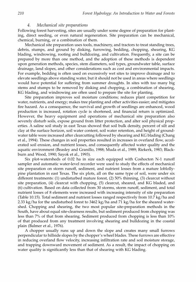
210 Forest Hydrology: An Introduction to Water and Forests
4. Mechanical site preparationsFollowing forest harvesting, sites are usually under some degree of preparation for plant-ing, direct seeding, or even natural regeneration. Site preparation can be mechanical,chemical, burning, or a combination of them.
Mechanical site preparation uses tools, machinery, and tractors to treat standing trees,debris, stumps, and ground by disking, furrowing, bedding, chopping, shearing, KGblading, windrowing, rooting and bulldozing, and cultivation. Frequently, a site can beprepared by more than one method, and the adoption of these methods is dependentupon generation methods, species, stem diameters, soil types, groundwater table, surfacedrainage, land slopes, and other considerations such as cost and environmental impacts.For example, bedding is often used on excessively wet sites to improve drainage and toelevate seedlings above standing water, but it should not be used in areas where seedlingswould have potential for suffering from summer droughts. In sites with too many bigstems and stumps to be removed by disking and chopping, a combination of shearing,KG blading, and windrowing are often used to prepare the site for planting.
Site preparation improves soil moisture conditions; reduces plant competition forwater, nutrients, and energy; makes tree planting and other activities easier; and mitigatesfire hazard. As a consequence, the survival and growth of seedlings are enhanced, woodproduction is increased, rotation cycle is shortened, and financial return is optimized.However, the heavy equipment and operations of mechanical site preparation alsoseverely disturb soils, expose ground from litter protection, and alter soil physical prop-erties. A saline soil study in east Texas showed that soil bulk density, percent of silt andclay at the surface horizon, soil water content, soil water retention, and height of ground-water table were increased after clearcutting followed by shearing and KG blading (Changet al., 1994). These changes in soil properties resulted in increases in overland flow, accel-erated soil erosion, and nutrient losses, and consequently affected water quality and theaquatic environment (Beasley and Granillo, 1988; Muda et al., 1989; Riekerk, 1983; Black-burn and Wood, 1990; Sayok et al., 1993).
Six plot-watersheds of 0.02 ha in size each equipped with Coshocton N-1 runoffsampler and automatic water-level recorder were used to study the effects of mechanicalsite preparation on storm runoff, sediment, and nutrient losses from a mature loblolly-pine plantation in east Texas. The six plots, all on the same type of soil, were under sixdifferent treatments: (1) undisturbed mature forest, (2) 50% thinning, (3) clearcut withoutsite preparation, (4) clearcut with chopping, (5) clearcut, sheared, and KG bladed, and(6) cultivation. Based on data collected from 30 storms, storm runoff, sediment, and totalnutrient losses of 8 elements were increased with increasing intensity of site preparation(Table 10.15). Total sediment and nutrient losses ranged respectively from 10.7 kg/ha and2.33 kg/ha for the undisturbed forest to 3462 kg/ha and 71 kg/ha for the sheared water-shed. Chopping and shearing, the two most popular site-preparation methods in theSouth, have about equal site-clearness results, but sediment produced from chopping wasless than 7% of that from shearing. Sediment produced from chopping is less than 10%of that produced from any treatment involving shearing and bulldozing in the coastalplain (Balmer et al., 1976).
A chopper usually runs up and down the slope and creates many small furrowsperpendicular to hillside slopes by the chopper’s wheel blades. These furrows are effectivein reducing overland flow velocity, increasing infiltration rate and soil moisture storage,and trapping downward movement of sediment. As a result, the impact of chopping onwater quality is significantly less than that of shearing with KG blading.
1363_C10_fm Page 210 Wednesday, December 4, 2002 7:43 AM
Chapter ten: Forests and streamflow 211
C. Cumulative watershed effects
Frequently a forest is managed for more than one purpose and by adopting more thanone activity to reach each purpose. These multiple uses and management activities arenot only common in practice but also mandated on federal lands by laws such as theMultiple-Use and Sustained Yield Act of 1960, the National Forest Management Act of1976, and the Clean Water Act of 1977 (Sidle and Hornbeck, 1991). The effects of multipleactivities on streamflow are obviously greater than effects from any single activity. How-ever, research on water quality and quantity is traditionally concerned with the effects ofindividual land uses and activities, and studies on the combination and interaction ofmultiple activities are rare.
Cumulative watershed effects refer to the additive, combined, and interactive impactscreated by additional activities through time and space. A cumulative-effects study of landuse on water quality along a fifth-order stream in western North Carolina showed thatstreamflow with low concentrations of chemical and biotic constituents, physical variables,and cations were predominantly associated with forested conditions in upper streams.Most variables were slightly increased downstream, and the increases were pronouncedduring stormflow stages (Bolstad and Swank, 1997). In the H.J. Andrews ExperimentalForest, Oregon, a 25-year study on landslides and soil erosion showed that the averageerosion rate was 2.51 m3/ha/year. Although forest roads cover only 5% of the entire area,they contribute 51% of the annual erosion losses. Landslides and accelerated erosion inclearcut areas (26% of the total area) accounted for 25% of the erosion, and the other 24%came from the 69% forested area. In other words, the volume of slide material per unitarea moved from the roads was 30 times the rate of that in undisturbed forests and about10 times that in clearcut areas. In comparison, if a forest fire occurred on 3% of the
Table 10.15 Total Net Rainfall, Runoff, Sediment, and Nutrient Losses under 6 Forest Conditions from 30 Storms Observed between May 1980 and February 1981 in Forested East Texas
Variables Treatmentsa
a b c d e f
Net rainfall, mm 360 378 430 459 459 459Runoff, mm 7.4 17.0 41.7 81.4 137.3 119.0Sediment, kg/ha 10.7 17.1 155.8 265.0 3461.6 3423.4Nutrients, kg/hab
K 0.25 0.90 1.85 2.74 6.69 3.85Na 0.23 0.70 1.57 3.08 8.66 5.21Ca 0.36 1.55 1.47 3.07 10.83 6.13Mg 0.08 0.30 0.79 1.48 7.76 6.38NO3 + NO2 0.31 1.07 2.30 3.31 7.93 6.63TKN 0.44 2.22 5.24 3.62 10.86 7.74SO4 0.41 1.57 3.30 2.13 12.12 7.23PO4 0.20 0.36 1.70 1.90 5.72 3.73Total 2.33 8.57 18.18 21.23 70.58 46.65
a Treatments: a: undisturbed mature forest, b: 50% thinning, c: clearcutting without site preparation, d: clearcutand chopping, e: clearcut, sheared, and KG bladed, f: clearcut, clean till for cultivation.
b Covered 23 storms.
Source: Chang, M., Roth, F.A., II, and Hunt, E.V., Jr., 1982, Sediment production under various forest siteconditions, in Recent Development in the Explanation and Prediction of Erosion and Sediment Yield, Walling, D.E.,Ed.,. IAHS Publ. No. 137. pp. 13–22.
1363_C10_fm Page 211 Wednesday, December 4, 2002 7:43 AM
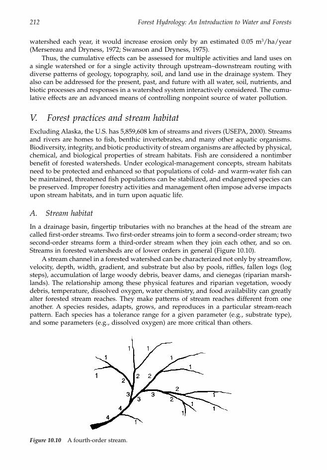
212 Forest Hydrology: An Introduction to Water and Forests
watershed each year, it would increase erosion only by an estimated 0.05 m3/ha/year(Mersereau and Dryness, 1972; Swanson and Dryness, 1975).
Thus, the cumulative effects can be assessed for multiple activities and land uses ona single watershed or for a single activity through upstream–downstream routing withdiverse patterns of geology, topography, soil, and land use in the drainage system. Theyalso can be addressed for the present, past, and future with all water, soil, nutrients, andbiotic processes and responses in a watershed system interactively considered. The cumu-lative effects are an advanced means of controlling nonpoint source of water pollution.
V. Forest practices and stream habitatExcluding Alaska, the U.S. has 5,859,608 km of streams and rivers (USEPA, 2000). Streamsand rivers are homes to fish, benthic invertebrates, and many other aquatic organisms.Biodiversity, integrity, and biotic productivity of stream organisms are affected by physical,chemical, and biological properties of stream habitats. Fish are considered a nontimberbenefit of forested watersheds. Under ecological-management concepts, stream habitatsneed to be protected and enhanced so that populations of cold- and warm-water fish canbe maintained, threatened fish populations can be stabilized, and endangered species canbe preserved. Improper forestry activities and management often impose adverse impactsupon stream habitats, and in turn upon aquatic life.
A. Stream habitat
In a drainage basin, fingertip tributaries with no branches at the head of the stream arecalled first-order streams. Two first-order streams join to form a second-order stream; twosecond-order streams form a third-order stream when they join each other, and so on.Streams in forested watersheds are of lower orders in general (Figure 10.10).
A stream channel in a forested watershed can be characterized not only by streamflow,velocity, depth, width, gradient, and substrate but also by pools, riffles, fallen logs (logsteps), accumulation of large woody debris, beaver dams, and cienegas (riparian marsh-lands). The relationship among these physical features and riparian vegetation, woodydebris, temperature, dissolved oxygen, water chemistry, and food availability can greatlyalter forested stream reaches. They make patterns of stream reaches different from oneanother. A species resides, adapts, grows, and reproduces in a particular stream-reachpattern. Each species has a tolerance range for a given parameter (e.g., substrate type),and some parameters (e.g., dissolved oxygen) are more critical than others.
Figure 10.10 A fourth-order stream.
1363_C10_fm Page 212 Wednesday, December 4, 2002 7:43 AM
Chapter ten: Forests and streamflow 213
1. Habitat parametersMany habitat parameters can affect the biological integrity of streams. Karr and Dudley(1981) grouped those parameters into five primary categories: water quality, flow regime,physical habitat, energy, and biotic interactions. The parameters that relate to flow regimeand physical habitat are discussed below.
a. Streamflow. Running water affects the transport and deposition of instreamparticles, streambed structure, plankton populations, and the ability of fish to feed (e.g.,extraction of nutrients in water current). A species must adapt to the flow conditions inwhich it colonizes. A relatively stable streamflow without extreme floods and droughts isa major factor for productive streams. Extreme high water can destroy available habitats,and fish may not be able to withstand the shear stress of the water. On the other hand,low summer flow could be the major factor limiting the abundance of many species,including coho salmon, anadromous rainbow, and cutthroat trout (Narver, 1971; Hicks etal., 1991a). Many forested headwater streams become intermittent during the summer,which makes fish susceptible to both instream predation and avian predation. Shallowstreams, especially those in open-canopy situations, tend to have higher temperatures,greater temperature fluctuation over time, and more energy for photosynthesis. Shadeand nutrient input from overhanging riparian vegetation seem to decrease with the widthof streams. Generally, large fish tend to prefer deep water while smaller fish live in shallowwater. Thus, creating pools and increasing riffle areas are often used as effective approachsfor enhancing rearing habitat for salmon and trout (Hall and Baker, 1982; Waters, 1995).
Although flow velocity and depth are important parameters of stream habitats, anumber of regional studies showed that streamflow velocity and depth were not signifi-cantly correlated with density, biomass, and catch-per-effort for smallmouth bass(M. dolomiece) and spotted bass (Micropterus punctulatus) in warmwater streams (McClen-don and Rabeni, 1987; Sowa and Rabeni, 1995; Tillma et al., 1998). This suggests that fishhave the ability to adapt to a variety of flow conditions, or that the microhabitat of theseparameters has not been properly assessed.
b. Temperature. Fish are ecothermic (cold-blooded); their internal temperaturesclosely follow external water temperatures. As a rule of thumb, a rise in temperature 1∞Cincreases metabolic rates in fish by 10%. Thus, as stream temperatures increase, fooddemand and dissolved oxygen demand also increase. This is compounded by the fact thatwarmer water holds less dissolved oxygen (and other gases) than cold water. Streamtemperatures suitable for fish depend on many factors, including species composition andlife-history stage. The spawning temperature, optimal temperature for growth, and max-imum tolerated temperature for Atlantic salmon (Salmo salar) are 0 to 8∞C, 13 to 15∞C, and16 to 17∞C, respectively. For rainbow trout (Salmo gairdneri), they are 4 to 10∞C, 20 to 21∞C,and 24∞C, (Moss, 1988). Changes in stream temperature beyond the optimum level cancause disease outbreaks, retard growth, stop migration, and cause death. However, highersummer water temperatures and accompanying lower dissolved oxygen levels seldomimpact fish such as spotted bass, largemouth bass, and bluegill sunfish in southern foreststreams like them impact salmonids in streams of the Northwest. This is because warm-water fish in the South have evolved mechanisms to cope with these factors (Rainwater,2001, personal communication). If streamflow in the headwaters is impeded by droughtor forest practices and it reaches the tolerance limits of temperature and oxygen require-ments, the ecosystem will be stressed regardless of the location.
c. Dissolved oxygen. Oxygen in water is required for respiration in fish and otheraquatic animals. It is supplied to the stream from the atmosphere through gas diffusion;
1363_C10_fm Page 213 Wednesday, December 4, 2002 7:43 AM
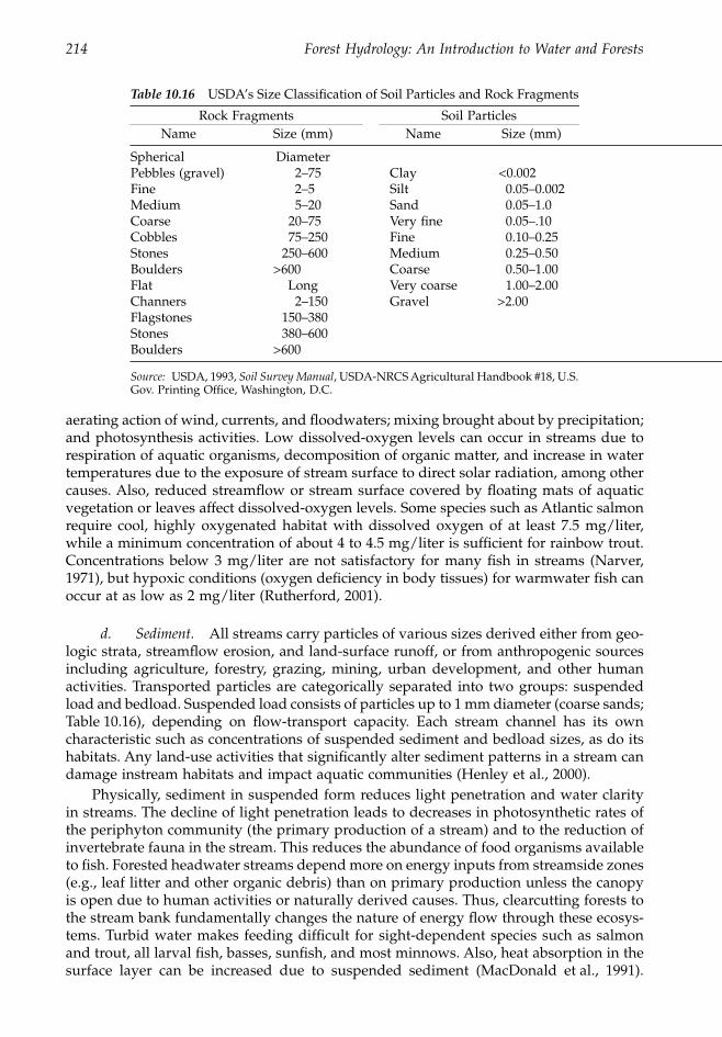
214 Forest Hydrology: An Introduction to Water and Forests
aerating action of wind, currents, and floodwaters; mixing brought about by precipitation;and photosynthesis activities. Low dissolved-oxygen levels can occur in streams due torespiration of aquatic organisms, decomposition of organic matter, and increase in watertemperatures due to the exposure of stream surface to direct solar radiation, among othercauses. Also, reduced streamflow or stream surface covered by floating mats of aquaticvegetation or leaves affect dissolved-oxygen levels. Some species such as Atlantic salmonrequire cool, highly oxygenated habitat with dissolved oxygen of at least 7.5 mg/liter,while a minimum concentration of about 4 to 4.5 mg/liter is sufficient for rainbow trout.Concentrations below 3 mg/liter are not satisfactory for many fish in streams (Narver,1971), but hypoxic conditions (oxygen deficiency in body tissues) for warmwater fish canoccur at as low as 2 mg/liter (Rutherford, 2001).
d. Sediment. All streams carry particles of various sizes derived either from geo-logic strata, streamflow erosion, and land-surface runoff, or from anthropogenic sourcesincluding agriculture, forestry, grazing, mining, urban development, and other humanactivities. Transported particles are categorically separated into two groups: suspendedload and bedload. Suspended load consists of particles up to 1 mm diameter (coarse sands;Table 10.16), depending on flow-transport capacity. Each stream channel has its owncharacteristic such as concentrations of suspended sediment and bedload sizes, as do itshabitats. Any land-use activities that significantly alter sediment patterns in a stream candamage instream habitats and impact aquatic communities (Henley et al., 2000).
Physically, sediment in suspended form reduces light penetration and water clarityin streams. The decline of light penetration leads to decreases in photosynthetic rates ofthe periphyton community (the primary production of a stream) and to the reduction ofinvertebrate fauna in the stream. This reduces the abundance of food organisms availableto fish. Forested headwater streams depend more on energy inputs from streamside zones(e.g., leaf litter and other organic debris) than on primary production unless the canopyis open due to human activities or naturally derived causes. Thus, clearcutting forests tothe stream bank fundamentally changes the nature of energy flow through these ecosys-tems. Turbid water makes feeding difficult for sight-dependent species such as salmonand trout, all larval fish, basses, sunfish, and most minnows. Also, heat absorption in thesurface layer can be increased due to suspended sediment (MacDonald et al., 1991).
Table 10.16 USDA’s Size Classification of Soil Particles and Rock Fragments
Rock Fragments Soil ParticlesName Size (mm) Name Size (mm)
Spherical DiameterPebbles (gravel) 2–75 Clay <0.002Fine 2–5 Silt 0.05–0.002Medium 5–20 Sand 0.05–1.0Coarse 20–75 Very fine 0.05–.10Cobbles 75–250 Fine 0.10–0.25Stones 250–600 Medium 0.25–0.50Boulders >600 Coarse 0.50–1.00Flat Long Very coarse 1.00–2.00Channers 2–150 Gravel >2.00Flagstones 150–380Stones 380–600Boulders >600
Source: USDA, 1993, Soil Survey Manual, USDA-NRCS Agricultural Handbook #18, U.S.Gov. Printing Office, Washington, D.C.
1363_C10_fm Page 214 Wednesday, December 4, 2002 7:43 AM
Chapter ten: Forests and streamflow 215
Biologically, high concentrations of suspended sediment can disrupt fish respiration andcause gill damage (Reynolds et al., 1989).
When sediment is deposited on the streambed, it can coat fish eggs and larvae, sealinterstices, and trap fry (for salmonids) in the gravel. These factors cause oxygen deficien-cies in gravel beds, inadequate removal of metabolities (free carbon and ammonia, toxicto aquatic organisms), and starvation of fry (only for salmonids). Recommendations ofsuspended sediment concentrations were less than 30 mg/liter for a high level and 100mg/liter for a moderate level of protection. A suspended sediment concentration of 488mg/liter was fatal to juvenile chinook salmon in Washington (Lloyd, 1987). However, inaddition to the concentration level, the duration of exposure is crucial in a stressedenvironment. Newcombe and MacDonald (1991) showed that the product of suspendedsediment concentration and duration of exposure was a much better indicator of effects(R2 = 0.64) than suspended sediment alone (R2 = 0.14).
e. Substrate. The substrate, or streambed to hydrologists, of a stream is composedof a variety of particles in various sizes, voids among particles, organic matter, and aquaticanimals and plants. It may be predominantly muddy, sandy, stony, or mixed, and may bestable or unstable. In headwater streams, particle sizes are generally larger (except coastalstreams in the southeastern U.S.), channels shallower, cross-sectional areas narrower,slopes greater, and surface rougher than those downstream (Morisawa, 1985). Streamswith braided channels are unstable, carry a great amount of bedload, and are severe inbank erosion. Streams with bedrock or bedrock-controlled waterways are stable and haveless erosion (Rosgen, 1996). In other words, streambeds dominated by large particles tendto be more stable in general than ones dominated by fine particles.
Substrate is the most biologically active zone in stream profiles. It is a site for eggdeposition and incubation, a source for food supplies, shelter for protection from preda-tors, and habitats for aquatic organisms. However, each aquatic species has its ownpreferred substrate; variations on species abundance and diversity are great among sub-strates. A mixed substrate of sand, gravel, and large particles (e.g., rubble, cobble, boulder)usually supports the greatest number of species. Lowland streams with silt and clay bedstend to have less diversity of aquatic animals, but may be a favorable site for aquaticplants and planktonic organisms (Gordon et al., 1993). Salmonids require a substrate withclean, mixed, stable gravel of 1 to 15 cm in diameter, small amounts of fine sediments,and high concentrations of dissolved oxygen (Narver, 1971). Gravel and gravel pluscobble, providing cover for resting and protection of newly hatched larvae, are dominanttypes of substrate in paddlefish (Polyodon spathula) spawning areas (Crance, 1987). In theSoutheast, where there is a lack of large substrates such as boulders and bedrock ledges,woody debris becomes an important habitat component for smallmouth bass and spottedbass (Tillma et al., 1998). A study of population characteristics of smallmouth bass androck bass in Missouri found that large substrate, undercut banks, and aquatic vegetationwere the three most important habitat parameters among 32 parameters studied(McClendon and Rabeni, 1987).
f. Pools. Pools are the concave sections along a stream channel where flowvelocity is lower, water is deeper, and substrate particles are finer than in adjacent rifflesor runs. Thus, when stream channels have no flow in summer, pools can still providewater for fish to survive and serve as sites for escape from intense predation. Deep slow-moving pools are helpful for salmonid survival under harsh winter conditions.
Pools can be created by channel erosion and deposition processes, bank undercut,debris dams, beaver dams, logjams, or other events. They are essential habitats for streamfish, especially larger predatory species such as trout, and a variety of pools is required
1363_C10_fm Page 215 Wednesday, December 4, 2002 7:43 AM
216 Forest Hydrology: An Introduction to Water and Forests
to provide habitats for different species and age classes of fish. Thus, species abundanceand diversity are often related to the area, volume, depth, number, type, and frequencyof pools. Land-use and management activities that cause severe soil erosion and streamsedimentation problems can reduce the depth, volume, and size of pools. Creating ade-quate pools in streams is a major effort in many programs for rehabilitating and enhancingstream habitat (Reeves and Roelofs, 1982; Seehorn, 1992).
Often a pool is followed by a convex streambed section, called a riffle, where currentis rapid, water is shallow, and sediment is dominated by coarse particles. Riffles arepredominately inhabited by young and small fish. The sequence of pool–riffle along astream channel provides a great diversity of channel morphology and aquatic habitats.
g. Cover. The shading and sheltering effects of cover are essential to streamsalmonids and other species. They can be in the form of streamside or submerged vege-tation, undercut banks, logs, rocks, floating debris, turbulence, deep water, or turbidity(Bjornn and Reiser, 1991). Fish use cover for protection from disturbance and predation,feeding stations, food sources, wintering, and resting. Streams under overhanging vege-tation are cooler in summer and warmer in winter, and have more nutrient input fromvegetation. Cooler temperature under the shaded area imply greater dissolved oxygen, aparameter important to fish activities.
In Kansas streams, root-wad and undercut bank areas were found to be the two mostimportant habitat components affecting the density and biomass of spotted bass(M. punctulatus) among 34 studied parameters (Tillma et al., 1998). Underwater observationsin southern Ontario, Canada, noted that both brook trout (Salvelinus fontinalis) and browntrout (Salmo trutta) preferred holding positions beneath submerged cover structures ratherthan under above-water structures or uncovered control forms (Cunjak and Power, 1987).
2. Habitat-rating indexesAlthough many parameters can affect the variation of stream habitats (one study involved43 parameters; Wang et al., 1998), some are more critical than others for a given speciesor community. Knowing those critical parameters and their impacts on stream biologicalcommunities is essential in formulating management, protection, and enhancement pro-grams for aquatic resources. They provide resource managers with adequate informationfor decision-making without requiring complex data collection in the field. This is anadvantage because managers often do not have time and funding to conduct rigorousdata collection and analyses. This leads scientists to develop habitat indexes or modelsinvolving only a few key and sensitive parameters. Once developed, they can be used for:(1) spatial and temporal comparisons and communication with other streams, (2) con-structing habitat maps in poorly sampled areas, (3) evaluating impact scenarios of regu-latory alternatives, (4) identifying and prioritizing areas for conservation actions, and(5) predicting or assessing impacts of environmental change (Wang et al., 1998; Brownet al., 2000).
Habitat indexes are simple mathematical expressions to relate habitat quality as afunction of one or more environmental parameters. Values of environmental parametersused in mathematical calculations may be based either on assigned ranges given byprofessional judgment (0 to 1, or others, depending on how favorable the range is forsurvival, growth, and reproduction of a given species) or on actual field observations. Thederived indexes result in a single value to represent habitat quality or conditions for aparticular species or a life stage, or an entire fish community at a specified geographicalscale. Some developed models include: habitat suitability index (HSI) by USEPA (1981)and USFWS (1981), rapid bioassessment protocols (RBP) by USEPA (Plafkin et al., 1989),habitat quality index (HQI) in Missouri (Fajen and Wehnes, 1982), qualitative habitat
1363_C10_fm Page 216 Wednesday, December 4, 2002 7:43 AM
Chapter ten: Forests and streamflow 217
evaluation index (QHEI) in Ohio (Rankin, 1989), fish habitat rating system (SHRS) inWisconsin (Wang et al., 1998), habitat suitability curve (HSC) in Kansas and Oklahoma(Layher and Maughan, 1987), and sediment stress index in British Columbia, Canada(Newcombe and MacDonald, 1991). Geographic patterns can be discerned from applyingthe indexes and GIS techniques, which provide managers with another tool to help for-mulate management plans.
B. Forest practices
Forestry practices have potential impacts on stream habitats and aquatic communities by:(1) altering the structure and composition of the riparian vegetation, (2) allowing moresolar radiation to reach stream surfaces, (3) generating more sediment to stream channels,and (4) decreasing the amount of large woody debris in streams. Stream-habitat parame-ters that are involved in the alteration may include supplies of organic matter, streamtemperature, the stability of channel morphology, substrates, sediment, plant nutrients,dissolved oxygen, debris and large woody debris, pools, covers, and others.
1. On riparian vegetationThe removal of riparian vegetation can affect food supplies of the stream through:(1) cutting down supplies of leaves, needles, twigs, and wood to streams, (2) shifting thecomposition of organic matter inputs from the more decay-resistant coniferous materialto more decomposable deciduous material, and (3) reducing the amount of insects andother animal wastes that drop from canopies. These are of particular importance in small-forested streams where riparian vegetation virtually covers the water surface and thelimited aquatic photosynthesis cannot provide the needed energy base for aquatic inver-tebrates, bacteria, and fungi. Here, as biologist Dr. Fred L. Rainwater (personal commu-nication December 11, 2001) has stated, heterotropic (getting energy and nutrients fromother organisms) dominated ecosystem functions in these headwaters. The fish living inthis habitat are omnivores (eating both plants and animals) and invertivores (invertebrateeating), and seldom (perhaps a single species) piscivores (fish eating). The reliance ofriparian source of organic particulates declines as the stream width increases and thesunlight strikes the stream surface. It then promotes autotropic (organisms making theirown food) dominance over heterotropic. The individual sizes of fish increase, and pisci-vores become more common. Management objectives need to determine the balancebetween decreases in organic-matter supply and increases in primary and secondaryproduction in the stream.
Besides a source of food supplies to streams, riparian vegetation provides falling trees,coarse woody debris, shade, and cover important to stream habitats. In the West, Californiagolden trout (Oncorhynchus mykiss aguabonita) more often selected undercut bank, aquaticvegetation, and sedge and avoided bare and collapsed banks (Matthews, 1996). Variabilityof the density and biomass of smallmouth bass and rock bass (Ambloplites rupestris) wasalso associated with aquatic vegetation in Missouri streams (McClendon and Rabeni, 1987).Of the three cover parameters important to trout habitats, overhead riparian vegetationcover explained a greater amount of variation than rubble-boulder-aquatic vegetation anddeepwater areas did in trout population size in southeast Wyoming (Wesche et al., 1987).
2. On water temperature
a. Variations. Timber-harvesting operations often expose streams in headwaterwatersheds to direct solar radiation, a factor that can cause significant changes in streamtemperature regimes. These changes include higher maximum and minimum tempera-
1363_C10_fm Page 217 Wednesday, December 4, 2002 7:43 AM
218 Forest Hydrology: An Introduction to Water and Forests
tures in the summer, greater diurnal temperature fluctuations, and longer durations fortemperatures to remain above a threshold value (Hewlett and Fortson, 1982; Rishel et al.,1982; Beschta and Taylor, 1988). The effects are most significant in small streams in whichstreamflows are low and surface areas in relation to flow volumes are large. Studiesshowed that forest harvesting increased average daily maximum stream temperature 1.2to 7.2∞C in the eastern U.S. and 0.6 to 8.0∞C in the western U.S. (Stednick, 2000). Forsummer maximum, increases were reported of more than 10∞C in central Pennsylvaniaand 16∞C in western Oregon. However, at higher elevations in northern latitudes, winterstream temperatures may be reduced due to the loss of insulation from riparian vegetationand the increase in outgoing longwave radiation from the stream (Beschta et al., 1987).Both temperature increases in summer and decreases in winter have negative impacts onbiological communities.
b. Management. In small-forested streams, convective, conductive, and evapora-tive heat-transfer processes at the water surface are insignificant due to very low windmovement (Brown, 1980). This means that solar radiation striking the water surface is themajor source of heat for small streams. The energy received from the sun will not bedissipated to surrounding areas. It will be stored in the stream and cause increases instream temperature. On the other hand, if a zone of riparian vegetation is lifted to shadethe stream surface, it prevents stream surfaces from direct exposure to solar radiation, andthe stream temperature is not likely to be affected by clearcutting.
The length of shadow cast over the stream by riparian vegetation is affected by theheight of vegetation, the orientation of stream azimuth in respect to the sun, solar altitude(affected by hour of the day and season), and geographical location. Although not man-agerial, shadow cast by streambank (especially for trench-typed streams) or topographyis as effective as vegetation. Equations 8.11, 8.12, and 8.13 can be used to calculate thelength of shadow cast by tree belts or streambank. For estimating the length of shadowrequired to completely span the stream, or the so called “stream effective width, We,” thefollowing equations can be used (Currier and Hughes, 1980):
We = Wa/sin b (10.36)
Sin b = sin[180 – Ástream azimuth – sun azimuthÁ] (10.37)
where Wa is the actual stream width and b is the acute angle between stream azimuth andazimuth of the sun. At lat. 40∞N on August 12, the sun’s azimuth at 9 a.m. is 110∞(Figure 8.4). If the azimuth of a particular stream is 235∞ and the actual stream widthWa = 3 m, then We = (3 m)/[sin (180 - Á 235 - 110 Á)] = 3.66 m, or it requires a shadow of3.66 m long to cross the stream surface. For actual width to be equal to effective width, itrequires sin b = 1, or b = 90∞, meaning that the sun and stream are perpendicular. It is thesmallest value of We. As the acute angle b decreases, We increases; We will reach infinitywhen b = 0, or where the sun and stream lie parallel to each other. Thus, the potentialimpact of streamside cutting on water temperature is greater for smaller streams becausea greater surface area of small streams is more easily shaded by trees.
If additional heat DH (in cal cm-2 min-1) is received at the stream surface due to theremoval of riparian vegetation, its effect on stream temperature can be calculated by(Brown, 1980):
Dt = 0.00017 (DH)(A)/Q (10.38)
1363_C10_fm Page 218 Wednesday, December 4, 2002 7:43 AM
Chapter ten: Forests and streamflow 219
where Dt is the increase in stream temperature in ∞C, A is surface area of the stream in m2,Q is stream discharge in m3 sec-1, and 0.00017 is a constant to convert discharge m3 sec-1
into g min-1. The value DH should represent net radiation in which solar radiation, streamreflection, and the exchange of longwave radiation between the stream and the air shouldall be considered. However, using solar radiation as the substitute for net radiation, DHwas sufficient in several small streams in Oregon (Brown et al., 1971). The stream surface(area A) should include only the portion affected by the removal of riparian vegetation.Procedures for shade measurements in the field are given by Bartholow (1989).
c. Impacts. Increases in stream temperature due to the removal of riparian veg-etation generally stimulate primary production by microbial communities, algae, andinvertebrates (Gregory et al., 1987). At the Coweeta Hydrologic Laboratory, North Caro-lina, invertebrate taxonomic diversity increased in the stream immediately after clearcut-ting of a forested watershed, and benthic invertebrate abundance was three times higher.Biomass and production were two times higher following 16 years in succession thanthose of the adjacent control watershed (Swank et al., 2001). Higher production levels ingreen algae and grazer invertebrates suggest higher levels of food available for fish.However, the elevated temperature is accompanied by: (1) an increase in decompositionrates of organic matter by microbial activities that may lead to a deficiency of organicmatter in certain periods of time and (2) a decrease in dissolved oxygen levels that cancause stress, disease, and mortality to fish. Coupling these fast microbial activities with areduction in organic matter inputs from riparian vegetation may offset the increasedprimary productivity in streams to a significant degree.
In the Northwest, increased summer temperatures could affect salmonids by alteringhabitat suitability for rearing, upstream migration while increasing susceptibility to dis-ease, reducing metabolic efficiency, and shifting the competitive advantage of salmonidover nonsalmonid species (Beschta et al., 1987). Decreases in winter temperature mayslow down egg development and increase the possibility of surface ice formation (Hickset al., 1991b).
3. On sediment
a. Variations and impacts. Stream habitat can be impaired by additional sedimentinduced by forest practices such as forest roads, clearcutting, site preparations, and burn-ing. Annual average sediment concentrations in most forested streams are less than10 mg/liter, while stormflows are up to 100 mg/liter (Binkley and Brown, 1993). However,maximum increases in sediment concentrations caused by forest practices had beenreported to be 56,000 JTU at Fernow Experimental Watersheds near Parsons, West Virginiaand 14,949 mg/liter in northern Mississippi in the East and 7,670 mg/liter at AlseaExperimental Watersheds near Toledo, Oregon, in the West (Table 10.17). Average increasesin the first posttreatment year ranged from 300 to 900 mg/liter in general and, as anextreme case, from 2127 mg/liter in the control site to over 2800 mg/liter in the treatmentin northern Mississippi. The variations reflected soil and topographic conditions of theforest activities, weather conditions during the operations, the intensity of soil distur-bances, and with or without prevention measures.
Increased sediment in streams can affect stream habitats in several ways. They include:(1) altering channel morphology important to aquatic lives such as pools, riffles, spawninggravel, flow obstructions (barriers to fish migration), and side channels extended from thestream’s edge (Chamberlin et al., 1991), (2) reducing the abundance of food organisms suchas benthic invertebrates and periphyton available to the fish (Newcombe and MacDonald,1991), and (3) degrading gravel quality and strata composition important to spawning and
1363_C10_fm Page 219 Wednesday, December 4, 2002 7:43 AM
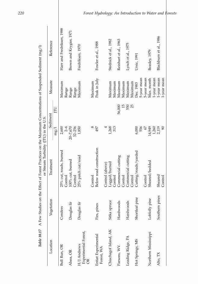
220 Forest Hydrology: An Introduction to Water and Forests
Tabl
e 10
.17
A F
ew S
tud
ies
on t
he E
ffec
t of
For
est
Prac
tice
s on
the
Max
imum
Con
cent
rati
ons
of S
uspe
nded
Sed
imen
t (m
g/l)
or
Str
eam
Tur
bid
ity
(JT
U)
in t
he U
.S.
Loc
atio
nV
eget
atio
nTr
eatm
ent
Sed
imen
tM
easu
reR
efer
ence
mg/
lJT
U
Bul
l Run
, OR
Con
ifer
s25
% c
ut, r
oad
s, b
urne
d2,
600
Max
imum
Har
r an
d F
red
riks
en, 1
988
Con
trol
2–6
Ran
geA
lsea
, OR
Dou
glas
fir
100%
cut
, bur
ned
20–7
,670
Ran
geB
row
n an
d K
rygi
er, 1
971
Con
trol
32–2
56R
ange
H/
J A
ndre
ws
Exp
erim
enta
l For
est,
OR
Dou
glas
fir
25%
pat
ch c
ut/
road
1,85
0M
axim
umFr
edri
ksen
, 197
0
Con
trol
8M
axim
umE
ntia
t E
xper
imen
tal
Fore
st, W
AFi
rs, p
ines
Bel
ow r
oad
con
stru
ctio
n49
7Pe
ak in
Jul
yFo
wle
r et
al.,
198
8
Con
trol
(ab
ove)
4C
hiac
hago
f Is
land
, AK
Sitk
a sp
ruce
Log
ged
/bu
rned
1,26
8M
axim
umSt
edni
ck e
t al.,
198
2C
ontr
ol31
3M
axim
umPa
rson
s, W
V.H
ard
woo
ds
Com
mer
cial
cut
ting
56,0
00M
axim
umR
einh
art
et a
l., 1
963
Con
trol
15M
axim
umL
ead
ing
Rid
ge, P
AH
ard
woo
ds
Com
mer
cial
cut
ting
550
Max
imum
Lync
h et
al.,
197
5C
ontr
ol25
Max
imum
Hot
Spr
ings
, MS
Shor
tlea
f pi
neC
utti
ng/
road
s/ya
rded
6,00
0D
ec. 1
983
Urs
ic, 1
991
556
5-ye
ar m
ean
Con
trol
675-
year
mea
nN
orth
ern
Mis
siss
ippi
Lob
lolly
pin
eSh
eare
d/
bed
ded
14,9
49M
ax. m
onth
Bea
sley
, 197
91,
260
1-ye
ar m
ean
Alt
o, T
XSo
uthe
rn p
ines
Shea
red
2,11
91-
year
mea
nB
lack
burn
et
al.,
1986
Con
trol
901-
year
mea
n
1363_C10_fm Page 220 Wednesday, December 4, 2002 7:43 AM
Chapter ten: Forests and streamflow 221
rearing habitats (Waters, 1995). Frequently, the majority of sediment delivered to streamscomes from one or a few major storms. The excessive runoff not only carries a great dealof sediment from forest management sites to stream channels but also causes severe bankerosion and bed scouring. As a result, channel forms can be altered, deposited sedimentredistributed, stream bank destabilized, and original habitats destroyed.
b. Buffer strips. Many BMPs have been proposed to reduce sediment productionfrom forest practices. Buffer strips are one of the most effective and have become a standardstrategy in forest operations. Buffer strips, or streamside management zones (SMZs), arezones of vegetation left along a stream bank to protect stream sediment and water qualityfrom forest practices. The effectiveness of an SMZ can be illustrated by a study conductedat 57 stations in 50 northern California streams. The study showed that the diversity ofmacroinvertebrate communities in streams with buffers (≥30 m) could not be distinguishedfrom those at control sites, but were significantly greater than in streams without bufferstrips (Newbold et al., 1980).
Buffer strips require a width greater than the distance sediment can move downslope.Sediment-travel distance is affected mainly by land slope, overland flow velocity anddepth, particle size, slope shape, and surface roughness. Predicting the distance of sedi-ment movement is difficult because of the interactions among variables (Seyedbagheri,1996). Many federal and state agencies have provided guidelines for the width of SMZ(U.S. Forest Service, 1984; Tennessee Valley Authority, 1990). The guidelines generallyrecommend widths that range from 10 to 100 m and wider for watersheds of steeper slopesand for protection of municipal water supplies. In the southern Appalachians, minimumSMZ widths for graded and graveled forest roads without brush barriers on the forestfloor can be estimated by the equation (Swift, 1986):
SMZ = 13 + 0.42 S (10.39)
where SMZ is in meters and S is slope in percent. If there are brush barriers on the forestfloor, the minimum width of SMZ is reduced to:
SMZ = 10 + 0.12 S (10.40)
For a 30% slope with no brush barriers on the floor, the minimum width of the SMZ is26 m, while a similar slope with brush barriers reduces the width of the SMZ to 14 m.
Buffer strips are subject to damage due to wind effect, logging, fire, or disease. Failuresof buffer strips jeopardize streamside-management objectives and watershed-manage-ment programs. In the Cascade Mountains of western Oregon, a study on 40 streamsidebuffer strips showed that wind damage accounted for nearly 94% of timber-volume loss(Steinblums et al., 1984). Thus, SMZ needs to be wider in wind-prone regions and forspecies susceptible to windthrow.
4. On large woody debris
a. Variations. Riparian trees deliver organic matter and debris continuously tothe stream throughout their succession stages. Any woody material with diameter greaterthan 10 cm and length greater than 1 m is generally considered large wood debris (LWD)(Meehan, 1991). The amount of large woody debris is usually greater in small streams,streams with finer substrates, and streams with greater riparian tree density. However,the length and diameter of LWD increase with stream size. Large pieces of woody debrisare difficult to flush out by flows, stay in the channel longer, and have greater impacts on
1363_C10_fm Page 221 Wednesday, December 4, 2002 7:43 AM
222 Forest Hydrology: An Introduction to Water and Forests
stream morphology, flow movement, and habitats for small streams compared to largestreams. In the Pacific Northwest, LWD covers as much as 50% of the channel in first- andsecond-order streams and 25% in third- and fourth-order streams (Sedell et al., 1988). Someconiferous LWD, depending on the transport capacity of streams and the resistance abilityto decomposition, breaking, and abrasion, have been in channels of the Pacific Northwestfor more than 200 years (Swanson et al., 1976).
b. Impacts. Traditionally, LWD has been considered a physical barrier to fishmigration, a blockage to floodwater movement, a retainer for sediment deposition, aconsumer for dissolved oxygen, and a supplier of certain compounds toxic to stream biota.These negative impacts have led to the removal of LWD from streams and rivers to allowfish migration, to reduce flood hazards, and to improve stream-habitat quality as a generalpractice through the early 1980s (MacDonald et al., 1993). More recent studies showedthat LWD is an important part of the stream morphology–habitat system.
LWD affects channel meandering and bank stability, creates a greater variation instream width and channel gradient, forms pools and waterfalls, and regulates the storageand routing of sediment. However, these impacts on the landscape are variable in degreedue to the position, orientation, size, volume, and frequency of LWD in stream channels(Bisson et al., 1987; Sedell et al., 1988). Biologically, LWD provides fish populations withdiversified habitats, organic matter and energy required in the aquatic food web, cover,and pools as survival shelters during low flows in the summer. Timber harvesting andlogging of riparian trees often cause streams to: (1) decline in the amount and size of LWD,(2) decrease in pool frequency and size, (3) lose important habitat features, (4) reduce fish-population abundance, (5) increase in bank instability, (6) decline in insect-communitydiversity, and (7) have reduced benthic detritus (Bryant, 1980; Bilby, 1984; Carlson et al.,1990; Ralph et al., 1994). In the Pacific Northwest, the removal of riparian forests hasreduced sources of LWD to stream channels for several decades, causing LWD abundancein the channel to decline and remain low for 50 to 100 years after logging (Beechie et al.,2000). It then becomes a challenge to forest- and fishery-resource managers to decide howmuch and what kind of LWD is required to add to the stream as an adequate measurefor maintaining fish habitats.
ReferencesAdams, P.W., 1999, Timber harvesting and the soil resource: what does the science show? in Clearcut-
ting in Western Oregon, Oregon State University College of Forestry, Corvallis, OR, pp. 77–93.Adams, P.W. and Stack, W.R.,1989, Stream Water Quality After Logging in Southwest Oregon, PNW
87–400, U.S. Forest Service Pacific NW Station, Portland, OR.Arcement, G.J., Jr. and Schneider, V.R., 1989, Guide for Selecting Manning’s Roughness Coefficients
for Natural Channels and Flood Plains, Water-Supply Paper 2339, U.S. Geological Survey.Baker, M.B., Jr., 1984, Changes in streamflow in an herbicide-treated pinoy-juniper watershed in
Arizona, Water Resour. Res., 20, 1639–1646.Baker, M.B., Jr., 1986, Effects of Ponderosa pine treatments on water yield in Arizona, Water Resour.
Res., 22, 67–73.Balmer, W.E. et al., 1976, Site preparation — why and how, Forest Management Bulletin, USDA
Forest Service, State and Private Forestry, Atlanta, Georgia.Barnes, H.H., Jr., 1967, Roughness Characteristics of Natural Channels, Paper 1849, U.S. Geological
Survey.Bartholow, J.M., 1989, Stream Temperature Investigations: Field and Analytic Meth-ods, Bio. Rep. 89(17), U.S. Fish and Wildlife Service, National Ecological Research Center,Fort Collins, CO.
Bates, C.G. and Henry, A.J., 1928, Forest and Streamflow Experiments at Wagon Wheel Gap, Colo-rado, U.S. Weather Bureau, No. 30.
1363_C10_fm Page 222 Wednesday, December 4, 2002 7:43 AM
Chapter ten: Forests and streamflow 223
Beasley, R.S., 1976, Contribution of subsurface flow from the upper slopes of forested watershedsto channel flow, J. Soil Sci. Soc. Am., 40, 955–957.
Beasley, R.S., 1979, Intensive site preparation and sediment losses on steep watersheds in the GulfCoastal Plain, Soil Sci. Soc. Am. J., 43, 412–417.
Beasley, R.S. and Granillo, A.B., 1988, Sediment and water yields from managed forests on flat coastalplain sites, Water Resour. Bull., 24, 361–366.
Beechie, T.J. et al., 2000, Modeling recovery rates and pathways for woody debris recruitment innorthwestern Washington streams, North Am.J. Fisheries Manage., 20, 436–452.
Bengston, D.N. and Fan, D.P., 1999, The public debate about roads on the national forests: an analysisof the news media, 1994–98, J. For., 97, 4–10.
Beschta, R.L., 1998, Forest hydrology in the Pacific Northwest: additional research needs, J. Am.Water Resour. Assoc., 34, 729–741.
Beschta, R.L. et al., 1987, Stream temperature and aquatic habitat: fishery and forestry interactions,in Streamside Management: Forestry and Fishery Interactions, Salo, E.O. and Cundy, T.W., eds.,University of Washington, Inst. of Forest Resources Contribution, Seattle, pp. 191–232.
Beschta, R.L. and Taylor, 1988, R.L., Stream temperature increases and land use in a forested Oregonwatershed, Water Resour. Bull., 24, 19–25.
Bethlahmy, N., 1973, Water yield, annual peaks and exposure in mountainous terrain, J. Hydro., 20,155–169.
Betson, R.P., 1979, The Effects of Clear Cutting Practices on Upper Bear Creek Watersheds, Alabama,Rep. No. WR28–1–550–101, Tennessee Valley Authority, Div. Water Resour.
Bilby, R.E., 1984, Removal of woody debris may affect channel stability, J. For., 82, 609–613.Binkley, D. and Brown, T.C., 1993, Management Impacts on Water Quality of Forests and Ranglands,
General Tech. Rep. RM-239, Rocky Mountain Forest and Range Exp. Sta., U.S. Forest Service,Fort Collins, CO.
Binkley, D. and Brown, T.C., 1993, Forest practices as nonpoint sources of pollution in North America,Water Resour. Bull., 29, 729–40.
Bisson, P.A. et al., 1987, Large woody debris in forested streams in the Pacific Northwest: past,present, and future, in Streamside Management: Forestry and Fishery Interactions, Salo, E.O. andCundy, T.W., Eds., University of Washington, Inst. of For. Resour. Contribution No. 57, pp.143–190.
Bjornn, T.C. and Reiser, D.W., 1991, Habitat requirements of salmonids in streams, in Influences ofForest and Rangeland Management on Salmonid Fishes and Their Habitats, Meehan, W.R., Ed.,.Am. Fisheries Soc., Bethesda, MD, pp. 83–138.
Blackburn, W.H. and Wood, J.C., 1990, Nutrient export in stormflow following forest harvesting andsite preparation in East Texas, J. Environ. Qual., 19, 402–408.
Blackburn, W.H., Wood, J.C., and DeHaven, M.G., 1986, Storm flow and sediment losses from site-prepared forestland in east Texas, Water Resour. Res., 22, 776–784.
Bolstad, P.V. and Swank, W.T., 1997, Cumulative impacts of land use on water quality in a southernAppalachian watershed, J. Am. Water Resour. Assoc., 33, 519–533.
Borg, H., Stoneman, G.L., and Ward, C.G., 1988, The effect of logging and regeneration on ground-water, streamflow and stream salinity in the southern forest of western Australia, J. Hydrology,99, 253–270.
Brady, N.C., 1990, The Nature and Properties of Soils, MacMillan, New York.Bray, D.I., 1979, Estimating average velocity in gravel-bed rivers, J. Hydraulic Div., 105, 1103–1122.Brown, G.W. and Krygier, J.T., 1970, Effects of clearcutting on stream temperature, Water Resour.
Res., 6, 1133–1140.Brown, G.W. and Krygier, T. 1971, Clearcut logging and sediment production in the Oregon Coast
Range, Water Resour. Res., 7, 1 189–1198.Brown, G.W., Swank, G.W., and Rothacher, J., 1971, Water Temperature in the Streamboat Drainage,
Res. Paper PNW-119, USDA Forest Service, Pacific NW Forest Exp. Sta., Portland, OR.Brown, G.W., 1980, Forest and Water Quality, O.S.U. Book Stores, Corvallis, OR. Brown, S.K. et al., 2000, Habitat suitability index model for fish and invertebrate species in Casco
and Sheepscot Bays, Maine, North Am. J. Fisheries Manage., 20, 408–435.
1363_C10_fm Page 223 Wednesday, December 4, 2002 7:43 AM
224 Forest Hydrology: An Introduction to Water and Forests
Bryant, M.D., 1980, Evolution of Large, Organic Debris after Timber Harvesting: Maybeso Creek,1949 to 1978, Gen. Tech. Rep. PNW-101, USDA Forest Service.
Bureau of Land Management, 1987, Assessment of Water Conditions and Management Opportuni-ties in Support of Riparian Values: BLM San Pedro River Properties, Arizona, Project Com-pletion Report, USDI, BLM Service Center, Denver, CO.
Burton, T.A., 1997, Effects of basin-scale timber harvest on water yield and peak streamflow, J. Am.Water Resour. Assoc., 33, 1187–1196.
Busby, M.W., 1966, Annual Runoff of the Conterminous United States, USGS Hydro. Investigations,Atlas HA-212.
Carlson, J.Y., Andrus, C.W., and Froehlich, H.W., 1990, Woody debris, channel features, and macro-invertebrates of streams with logged and undisturbed riparian timber in northeastern Ore-gon, Can. J. Fisheries and Aquatic Sci., 47, 1103–1111.
Chamberlin, T.W., Harr, R.D., and Everest, F.H., 1991, Timber harvesting, silviculture, and watershedprocesses, in Influences of Forest and Rangeland Management on Salmonid Fishes and TheirHabitats, Meehan, W.R., Ed., Am. Fisheries Soc., Bethesda, MD, pp. 181–205.
Chang, M., 1982, Laboratory Notes: Forest Hydrology, Center for Applied Studies in Forestry, Collegeof Forestry, Stephen F. Austin State University, Nacogdoches, TX.
Chang, M. and Boyer, D.G., 1977, Estimates of low flows using watershed and climatic parameters,Water Resour. Res., 13, 997–1001.
Chang, M. and Lee, R., 1976, Adequacy of Hydrologic Data for Applications in West Virginia, Bulletin7, Water Res. Institute, West Virginia University., Morgantown, WV.
Chang, M., Macullough, J.D., and Granillo, A.B., 1983, Effects of land use and topography on somewater quality variables in forested East Texas, Water Resour. Bull., 19, 191–196.
Chang, M., Roth, F.A., II, and Hunt, E.V., Jr., 1982, Sediment production under various forest siteconditions, in Recent Development in the Explanation and Prediction of Erosion and Sediment Yield,Walling, D.E., Ed.,. IAHS Publ. No. 137. pp. 13–22.
Chang, M. and Sayok, A.K., 1990, Hydrologic responses to urbanization in forested La Nana Creekwatershed, in Tropical Hydrology and Caribbean Water Resources, Am. Water Resour. Assoc.,Herndon, VA, pp. 131–140.
Chang, M., Sayok, A.K., and Watterston, K.G., 1994, Clearcutting and shearing on a saline soil inEast Texas: impact on soil physical properties, in Proceedings of the 8th Biennial SouthernSilvicultural Research Conference, U.S. Forest Service Southern Research Station, Asheville, NC,pp. 209–214.
Chang, M. and Waters, S.P., 1984, Forests and other factors associated with streamflows in east Texas,Water Resour. Bull., 20, 713–719.
Chen, J.D., 1988, Subsurface stormflows in the highly permeable forested watersheds of southwest-ern British Columbia, J. Contaminant Hydro., 3, 171–191.
Chow, V.T., 1959, Open-Channel Hydraulics, McGraw-Hill, New York.Clark, G.M., Muller, D.K., and Mast, M.A., 2000, Nutrient concentrations and yields in undeveloped
stream basins of the United States, J. Am. Water Resour. Assoc., 36, 849–860.Cline, R.G., Haupt, H.F., and Campbell, G.S., 1977, Potential Water Yield Response Following
Clearcut Harvesting on North And South Slopes in Northern Idaho, Res. Pap. INT-191, U.S.Forest Service, Intermountain For. And Range Exp. Sta., Ogden, UT.
Coon, W.F., 1998, Estimation of Roughness Coefficients for Natural Stream Channels with VegetatedBanks, Water Supply Paper 2441, U.S. Geological Survey.
Cowan, W.L., 1956, Estimating hydraulic roughness coefficients, Agr. Eng., 37, 473–475.Crance, J.H., 1987, Habitat suitability index curves for paddlefish, developed by the Delphi tech-
nique, North Am. J. Fisheries Manage., 7, 123–130.Cunjak, R.A. and Power, G., 1987, Cover use by stream-resident trout in winter: a field experiment,
North Am. J. Fisheries Manage., 7, 539–544.Currier, J.B. and Hughes, D., 1980, Temperature, in An Approach to Water Resources Evaluation of Non-
Point Silvicultural Sources (A Procedural Handbook), U.S. Environ. Protection Agency, Environ.Res. Lab., Athens, GA, pp. VII i-v, 1–30.
Davis, E.A., 1993, Chaparral control in mosaic pattern increased streamflow and mitigated nitrateloss in Arizona, Water Resour. Bull., 29, 391–399.
1363_C10_fm Page 224 Wednesday, December 4, 2002 7:43 AM
Chapter ten: Forests and streamflow 225
Dingman, S.L. and Palaia, K.J., 1999, Comparison of models for estimating flood quantiles in NewHampshire and Vermont, J. Am. Water Resour. Assoc., 35, 1233–1243.
Douglas, J.E., 1983, The potential for water yield augmentation from forest management in theeastern United States, Water Resour. Bull., 19, 351–358.
Edmonds, R.L. and Blew, R.D., 1997, Trends in precipitation and stream chemistry in pristine old-growth forest watershed, Olympic National Park, Washington, J. Am. Water Resour. Assoc.,33, 781–793.
Egan, A.F., 1999, Forest roads: where soil and water don’t mix, J. For., 97, 18–22.Emmerich, W.E., 1998, Estimating prescribed burn impacts on surface runoff and water quality in
southeastern Arizona, in Proc., Rangeland Management and Water Resources, Potts, D.F., Ed.,AWRA, pp. 149–158.
EPA, 1999, National Recommended Water Quality Criteria — Correction, U.S. Environmental Pro-tection Agency, EPA 822-Z-99–001.
Eschner, A.R. and Larmoyeux, J., 1963, Logging and trout: four experimental forest practices andtheir effect on water quality, Progressive Fish-Culturist, 25, 59–67.
Fajen, O.F. and Wehnes, R.E., 1982, Missouri’s method of evaluating stream habitat, in Acquisitionand Utilization of Aquatic Habitat Inventory Information, Armantrout, B., Ed., Am. Fisheries Soc.,Western Division, Bethesda, MD, pp. 117–123.
Folliott, P.F. and Thorud, D.B., 1977, Water resources and multiple-use forestry in the Southwest,J. For., 75, 469–472.
Fowler, W.B., Anderson, T.D., and Helvey, J.D., 1988, Changes in Water Quality and Climate afterForest Harvest in Central Washington State, Res. Paper PNW-388, U.S. Forest Service, PacificNW For. and Range Exp. Sta.
Fowler, W.B., Helvey, J.D., and Felix, E.N., 1987, Hydrologic and Climatic Changes in Three SmallWatersheds after Timber Harvest, Tech. Rep. PNW-379, U.S. Forest Service, Pacific NW For.and Range Exp. Sta.
Fread, D.L., 1993, Flow routing, in Handbook of Hydrology, Maidment, D.R., Ed., McGraw-Hill, NewYork, pp. 10,1–36.
Fredriksen, R.L., 1970, Erosion and Sedimentation Following Road Construction and Timber Har-vesting on Unstable Soils in Three Small Western Oregon Watersheds, Research Paper PNW-104, USDA Pacific NW Forest and Range Exp. Stat., Portland, OR.
Gingras, D., Adamowski, K., and Pilon, P.J., 1994, Regional flood equations for the provinces ofOntario and Quebec, Water Resour. Bull., 30, 55–67.
Gluns, D.R. and Toews, D.A.A., 1989, Effects of a major wildfire on water quality in southeasternBritish Columbia, in Proc. Headwaters Hydrology, Woessner, W.W. and Potts, D.F., Eds., Am.Water Resour. Assoc., Bethesda, MD, pp. 487–99.
Gordon, N.D., McMahon, T.A., and Finlayson, B.L., 1993, Stream Hydrology, An Introduction forEcologists, John Wiley & Sons, New York.
Gottfried, G.J., 1983, Stand changes on a southwestern mixed conifer watershed after timber har-vesting, J. For., 81, 311–316.
Gottfried, F.J. and DeBano, L.F., 1991, Streamflow and Water Quality Responses to PreharvestPrescribed Burning in an Undisturbed Ponderosa Pine Watershed, in Effects of Fire in Man-agement of Southwestern Natural Resources, Gen. Tech. Rep. RM-191, USDA Forest Service.
Grace, J.M., III, 1999, Forest road side slopes and soil conservation techniques, J. Soil Water Conserv.,54, 96–101.
Green, R.E. and Ampt, G.A., 1911, Studies on soil physics: 1. Flow of air and water through soils,J. Agr. Sci., 4, 1–24.
Gregory, S.V. et al., 1987, Influences of forest practices on aquatic production, in Streamside Manage-ment: Forestry and Fishery Interactions, Salo, E.O. and Cundy, T.W., ed., University of Wash-ington Institute of Forest Resources Contributions, pp. 233–255.
Groeneveld, D.P. and Or, D., 1994, Water table reduced shrub-herbaceous ecotone: hydrologicalmanagement implications, Water Resour. Bull., 30, 911–920.
Gucinski, H. et al., Eds., 2001, Forest Roads: a Synthesis of Scientific Information, Gen. Tech, Rep.PNW-GTR-509, Forest Service Pacific NW Res. Sta., Portland, OR.
Gupta, R.S., 1989, Hydrology and Hydraulic Systems, Waveland Press, Prospect Heights, IL.
1363_C10_fm Page 225 Wednesday, December 4, 2002 7:43 AM
226 Forest Hydrology: An Introduction to Water and Forests
Hall, J.D. and Baker, C.O., 1982, Influence of Forest and Rangeland Management on AnadromousFish Habitat in Western North America: 12. Rehabilitating and Enhancing Stream Habitat,1. Review and Evaluation, Gen. Tech. Rep. PNW-138, USDA Forest Service, Pacific NW Forestand Range Exp. Sta., Portland, OR.
Hamilton, L.S. and King, P.N., 1983, Tropical Forested Watersheds: Hydrologic and Soil Response to MajorUses or Conversions, Westview Press, Boulder, CO.
Harr, R.D., 1976, Forest Practices and Streamflow in Western Oregon, Gen. Tech. Rep. PNW-49,USDA Forest Service, Pacific NW Forest and Range Exp. Sta.
Harr, R.D., 1983, Potential for augmenting water yield through forest practices in western Washing-ton and western Oregon, Water Resour. Bull., 19, 383–394.
Harr, R.D. and Fredriksen, R.L., 1988, Water quality after logging small watersheds within the BullRun Watershed, Oregon, Water Resour. Bull., 24, 1103–1111.
Harr, R.D., Fredriksen, R.L., and Rothacher, J., 1979, Changes in Streamflow Following TimberHarvest in Southwest Oregon, Forest Service Res. Paper PNW-249, Pacific Northwest Forestand Range Exp. Sta.
Harr, R.D. and McCorison, F.M., 1979, Initial effects of clearcut logging on size and timing of peakflows in a small watershed in western Oregon, Water Resour. Res., 15, 90–94.
Harr, R.D., Levno, A., and Mersereau, R., 1982, Streamflow changes after logging 130 year-oldDouglas-fir in two small watersheds, Water Resour. Res., 18, 637–644.
Heikurainen, L., 1967, Effect of cutting on the groundwater level on drained peatlands, in Interna-tional Symposium On Forest Hydrology, Sopper, W.E. and Lull, H.W., Eds., Pergamon Press,Elmsford, NY, pp. 345–354.
Henley, W.F. et al., 2000, Effects of sedimentation and turbidity on lotic wood webs: a concise reviewfor natural resource managers, Rev. Fisheries Sci., 8, 125–139.
Hershfield, D.N., 1961, Rainfall Frequency Atlas of the United States, U.S. Weather Bureau.Hewlett, J.D. and Fortson, J.C., 1982, Stream temperature under an inadequate buffer strip in the
Southeast Piedmont, Water Resour. Bull., 18, 983–988.Hewlett, J.D. and Hibbert, A.R., 1961, Increases in water yield after several types of forest cutting,
Int. Assoc. Sci. Hydro. Bull., 6, 5–17.Hewlett, J.D. and Troendle, C.A., 1975, Nonpoint and diffuse water resources: a variable source area
problem, in Proc., Watershed Management, ASCE, New York, pp. 21–46.Hibbert, A.R., 1969, Water yield changes after converting a forest catchment to grass, Water Resour.
Res., 5, 634–640.Hibbert, A.R., 1983, Water yield improvement potential by vegetation management on western
rangelands, Water Resour. Bull., 19, 375–381.Hibbert, A.R., Davis, E.A., and Knipe, O.D., 1982, Water yield changes resulting from treatment of
Arizona chaparral, in Proc. of Sym. on Dynamic and Management of Mediterranean-Type Ecosys-tems, June 22–26, 1981, San Diego, CA, U.S. Forest Service, Pacific SW For. and Range Exp.Sta., Berkeley, CA., pp. 382–389.
Hicks, B.J., Beschta, R.L., and Harr, R.D., 1991a, Long-term changes in streamflow following loggingin western Oregon and associated fisheries implications, Water Resour. Bull., 27, 217–226.
Hicks, B.J. et al., 1991b, Responses of salmonids to habitat changes, in Influences of Forest and RangelandManagement on Salmonid Fishes and Their Habitats, Meehan, W.R., Ed., Amer. Fisheries Soc.,Bethesda, MD, pp. 483–518.
Holstener-Jorgensen, H., 1967, Influence of forest management and drainage on groundwater fluc-tuations, in International Symposium on Forest Hydrology, Sopper, W.E. and Lull, H.W., Eds.,Pergamon Press, Elmsford, NY., pp. 325–333.
Hornbeck, J.W., 1973, Storm flow from hardwood-forested and cleared watersheds in New Hamp-shire, Water Resour. Res., 9, 346–354.
Hornbeck, J.W. et al., 1993, Long-term impacts of forest treatments on water yield: a summary fornortheastern USA, J. Hydrology, 150, 323–344.
Hornbeck, J.W., Pierce, R.S., and Federer, C.A., 1970, Streamflow changes after forest clearing inNew England, Water Resour. Res., 6, 1124–1132.
1363_C10_fm Page 226 Wednesday, December 4, 2002 7:43 AM
Chapter ten: Forests and streamflow 227
Ice, G.G., 1999, Streamflow and water quality: what does the science show about clearcutting inwestern Oregon, in Clearcutting in Western Oregon: What Does the Science Show? College ofForestry, Oregon State University, Corvallis, OR, pp. 55–74.
Ingebo, P.A., 1971, Suppression of channel-side chaparral cover increases stream- flow, J. Soil WaterConserv., 26, 79–81.
Jarrett, R.D., 1984, Hydraulics of high-gradient streams, J. Hydrau. Eng., 110, HY11, 1519–1539.Jobson, H.E. and Froehlich, D.C., 1988, Basic Hydraulic Principles of Open-Channel Flow, U.S.
Geological Survey Open-File Report 88–707.Johnston, R.A., 1984, Effects of Small Aspen Clearcuts on Water Yield and Water Quality, Res. Paper
INT-333, U.S. Forest Service, Intermountain For. and Range Exp. Sta., Ogden, UT.Karr, J.R. and Dudley, D.R., 1981, Ecological perspective on water quality goals, Environ. Manage.,
5, 55–68.Kellogg, L.D., Bettinger, P., and Edwards, R.M., 1996, A comparison of logging planning, felling,
and skyline yarding costs between clearcutting and five group-selection harvesting methods,West. J. Appl. For., 11, 25–31.
Keppeler, E.T. and Ziemer, R.R., 1990, Logging effects on streamflow: water yield and summer lowflows at Caspar Creek in northwestern California, Water Resour. Res., 26, 1669–1679.
Kidwell, M.R., Weitz, M.A., and Guertin, D.P., 1997, Estimation of Green-Ampt effective hydraulicconductivity for rangelands, J. Range Manage., 50, 290–299.
King, J.G., 1989, Streamflow Response to Road Building and Harvesting: A Comparison with theClearcut Area Procedure, Gen. Tech. Rep. INT- 401, U.S. Forest Service, Intermountain For.and Range Exp. Sta., Ogden, UT.
Kirpich, Z.P., 1940, Time of concentration of small agricultural watersheds, Civil Eng., 10, 362.Kochenderfer, J.N., 1970, Erosion Control on Logging Roads in the Appalachians, Pap NE-158, USDA
Forest Service Res., NE Forest Exp. Stat., Upper Darby, PA.Kochenderfer, J.M. and Aubertin, G.M., 1975, Effects of management practices on water quality and
quantity: Fernow Experimental Forest, West Virginia, in Municipal Watershed Management,Sym. Proc., U.S. Forest Service Gen. Tech. Rep. NE-13, pp. 14–24.
Layher, W.G. and Maughan, O.E., 1987, Spotted bass habitat suitability related to fish occurrenceand biomass and measurement of physiochemical variables, North Am. J. Fisheries Manage.,7, 238–251.
Lee, R., 1963, Evaluation of Solar Beam Irradiation as a Climatic Parameter of Mountain Watersheds,Hydro. Paper 2, Colorado State Univ., Fort Collins, CO.
Lewis, D.C., 1968, Annual hydrologic response to watershed conversion from oak woodland toannual grassland, Water Resour. Res., 4, 59–72.
Lewis, E.L. and Brendle, D.L., 1998, Relations of Streamflow and Specific Conductance Trends toReservoir Operations in the Lower Arkansas River, Southern Colorado, Water-Resour. Invest.Rep. 97–4239, USGS, Denver, CO.
Likens, G.E. et al., 1977, Biogeochemistry of a Forested Ecosystem, Springer-Verlag, Heidelberg.Limerinos, J.T., 1970, Determination of the Manning Coefficient from Measured Bed Roughness in
Natural Channels, Water Supply Paper 1898-B, U.S. Geological Survey.Linsley, R.K., Jr., Kohler, M.A., and Paulhus, J.L.H., 1975, Hydrology for Engineers, McGraw-Hill, New
York.Lloyd, D.S., 1987, Turbidity as a water quality standard for salmonid habitats in Alaska, North Am.
J. Fisheries Manage., 7, 34–45.Lusby, G.C., 1979, Effects of Converting Sagebrush Cover to Grass on The Hydrology of Small
Watersheds at Boco Mountain, Colorado, in Hydro. Effects of Land Use, U.S. GeologicalSurvey Water Supply Paper.
Lynch, J.A., 2001, personal communication, School of Forest Resources, Pennsylvania State Univer-sity, University Park, PA.
Lynch, J.A. and Corbett, E.S., 1990, Evaluation of best management practices for controlling nonpointpollution from silvicultural operations, Water Resour. Bull., 26, 41–52.
Lynch, J.A. and Corbett, E.S., Increasing summer storm peakflows following progressive forestclearcutting, unpublished report, School of Forest Resources, Pennsylvania State University,University Park.
1363_C10_fm Page 227 Wednesday, December 4, 2002 7:43 AM
228 Forest Hydrology: An Introduction to Water and Forests
Lynch, J.A., Corbett, E.S., and Sopper, W.E., 1980, Impact of forest cover removal on water quality,Res. Rep. 23–604, Pennsylvania State University Inst. for Res. on Land and Water Resour.,Univ. Park.
Lynch, J.A. et al., 1975, Penn State experimental watersheds, in Municipal Watershed Management,Sym. Proc., USDA Forest Service General Tech. Rep. NE-13, pp. 32–46.
MacDonald, L.H., Smart, A.W, and Wissmar, R.C., 1991, Monitoring Guidelines to Evaluate Effectsof Forestry Activities on Streams in the Pacific Northwest and Alaska, EPA 910/9–91–001,U.S. Environmental Protection Agency.
Matthews, K.R., 1996, Habitat selection and movement patterns of California golden trout in de-graded and recovering streams selection in the Golden Trout Wilderness, California, NorthAm. J. Fisheries Manage., 16, 579–590.
McBroom, M.W., Chang, M., and Cochran, M.C., 1999, Water quality conditions of streams receivingrunoff from land-applied poultry litter in East Texas, in Watershed Management to ProtectDeclining Species, Proc. of AWRA, Sakrison, R. and Sturtevant, R., Eds., Am. Water ResourceAssociation, Bethesda. MD, pp. 549–552.
McClendon, D.D. and Rabeni, C.F., 1987, Physical and biological variables useful for predictingpopulation characteristics of smallmouth bass and rock bass in an Ozark stream, North Am.J. Fisheries Manage., 7, 46–56.
McClurkin, D.C. et al., 1985, Water quality effects of clearcutting Upper Coastal Plain loblolly pineplantations, J. Environ. Qual., 14, 329–332.
McCuen, R.H., 1998, Hydrologic Analysis and Design, Prentice Hall, New York.McGuinness, C.L., 1964, Generalized Map Showing Annual Runoff and Productive Aquifers in the
Conterminous United States, Atlas HA-194, USGS Hydro. Investigations.Meehan, W.R., 1991, Influences of Forest and Rangeland Management on Salmonid Fishes and Their
Habitats, Amer. Fisheries Soc., Bethesda, MD.Megahan, W.F., 1972, Logging, erosion, and sedimentation, are they dirty words?, J. For., 70, 403–407.Megahan, W.F., King, J.G., and Seyedbagheri, K.A., 1995, Hydrologic and erosional responses of a
granitic watershed to helicopter logging and broadcast burning, Forest Sci., 41, 777–795.Mein, R.G. and Larson, C.L., 1971, Modeling Infiltration Component of the Rainfall-Runoff Process,
Bull. 43, Water Resour. Res. Center, University of Minnesota, Minneapolis.Mersereau, R.C. and Dryness, C.T., 1972, Accelerated mass wasting after logging and slash burning
in western Oregon, J. Soil Water Conserv., 27, 112–114.Molchanov, A.A., 1963, The Hydrological Role of Forests, Acad. Sci. USSR, Inst. Forest, Moscow (Tranl.
from Russian, OTS63–11089).Morisawa, M., 1985, Rivers, Longman, New York.Moss, B., 1988, Ecology of Fresh Waters, Man and Medium, 2nd ed., Blackwell Scientific, Oxford.Muda, A., Chang, M., and Watterston, K.G., 1989, Effects of six forest-site conditions on nutrient
losses in East Texas, in Proc. Headwaters Hydrology, Woessner, W.W. and Potts, D.F., Am. WaterResour. Assoc., Bethesda, MD, pp. 55–56.
Narver, D.W., 1971, Effects of logging debris on fish production, in Forest Land Uses and StreamEnvironment, Oregon State University, Corvallis, OR., pp. 100–111.
Newbold, J.D., Erman, D.C., and Roby, K.B., 1980, Effects of logging on macro-invertebrates instreams with and without buffer strips, Can. J. Fish Aquat. Sci., 37, 1076–1085.
Newcombe, C.P. and MacDonald, D.D., 1991, Effects of suspended sediments on aquatic ecosystems,North Am J. Fisheries Manage., 11, 72–82.
Omernik, J.M., 1976, The influence of Land Use on Stream Nutrient Levels, EPA-600/3–76–014, EPAEnviron. Res. Lab., Corvallis, OR.
Patric, J.H., and Reinhart, K.G., 1971, Hydrologic effects of deforesting two mountain watershedsin West Virginia, Water Resour. Res., 7, 1182–1188.
Peck, A.J. and Williamson, D.R., 1987, Effects of forest clearing on groundwater, J. Hydrology, 94,47–65.
Pereira, H.C., 1973, Land Use and Water Resources, Cambridge University Press, Cambridge.Pilgrim, M.P. and Cordery, I., 1993, Flood runoff, in Handbook of Hydrology, Maidment, D.R., Ed.,
McGraw-Hill, New York, pp. 9, 1–42.
1363_C10_fm Page 228 Wednesday, December 4, 2002 7:43 AM

Chapter ten: Forests and streamflow 229
Pitt, M.D., Burgy, R.H., and Heady, H.F., 1978, Influences of brush conversion and weather patternson runoff from a northern California watershed, J. Range Manage., 31, 23–27.
Plafkin, J.L. et al., 1989, Rapid Bioassessment Protocols for Use in Streamsand Rivers: BenthicMacroinvertebrates and Fish, EPA/444/4–89–001, U.S. Environmental Protection Agency.
Pritchett, W.L., 1979, Properties and Management of Forest Soils, John Wiley & Sons, New York.Rainwater, F.L., 2001, personal communication, Biology Department, Stephen F. Austin State Uni-
versity, Nacogdoches, TX.Ralph, S.C. et al., 1994, Stream channel condition and instream habitat in logged and unlogged
basins of western Washington, Can. J. Fisheries Aquatic Sci., 51, 37–51.Rankin, E.T., 1989, The Qualitative Habitat Evaluation Index (QHEI, Rationale, Methods, and Ap-
plication, Ohio Environ. Protection Agency, Division of Water quality Planning and Assess-ment, Ecological Assessment Section, Columbus, OH.
Rawls, W.J. et al., 1993, Infiltration and soil water movement, in Handbook of Hydrology, Maidment,D.R., Ed., McGraw-Hill, New York, pp. 5, 1–51.
Rawls, W.J., and Brakensiek, D.L., 1983, A procedure to predict Green and Ampt infiltration param-eters, in Proc., Am. Soc. of Agr. Eng. on Advan. in Infiltration, Chicago, IL, pp. 102–112.
Reeves, G.H. and Roelofs, T.D., 1982, Influence of Forest and Rangeland Management on Anadro-mous Fish Habitat in Western North America: 13. Rehabilitating and Enhancing StreamHabitat, 2. Field Application, Gen. Tech. Rep. PNW-140, USDA Forest Service, Pacific NWForest and Range Exp. Sta., Portland, OR.
Reich, B.M., 1972, The influence of percentage forest on design floods, in National Symposium onWatershed in Tranition, Am. Water Resource. Assoc., Urbana, IL, pp. 335–340
Reinhart, K.G., Eschner, A.R., and Trimble, G.R., Jr., 1963, Effect on Streamflow of Four ForestPractices in the Mountains of West Virginia, Res. Paper NE-1, US Forest Service, NortheasternFor. Exp. Sta., Upper Darby, PA.
Reinhart, K.J. and Trimble, G.R., 1962, Forest cutting and increased water yield, J. Am. Works Assoc.,54, 1464–1472.
Reuss, J.O. et al., 1993, Biogeochemical Fluxes in the Glacier Lakes Catchments, Research Paper RM-314, USDA Forest Service, Rocky Mountain Forest and Range Exp. Sta.
Reynolds, J.B., Simmons, R.C., and Burkholder, A.R., 1989, Effects of placer mining discharge onhealth and food of Arctic grayling, Water Resour. Bull., 25, 625–635.
Rich, L.R., and Gottfried, G.J., 1976, Water yields resulting from treatments on the Workman Creekexperimental watersheds in central Arizona, Water Resour. Res., 12, 1053–1060.
Riekerk, H., 1983, Impact of silviculture on flatwood runoff, water quality, and nutrient budget,Water Resour. Bull., 19, 73–79.
Riekerk, H., 1989, Influences of silvicultural practices on hydrology of pine flatwoods in Florida,Water Resour. Res., 25, 713–719.
Rishel, G.B., Lynch, J.A., and Corbett, E.S., 1982, Seasonal stream temperature changes followingforest harvesting, J. Environ. Qual., 11, 112–116.
Rosgen, D., 1996, Applied River Morphology, Wildland Hydrology, Pagosa Springs, CO.Rothacher, J., 1970, Increases in water yield following clear-cut logging in the Pacific West, Water
Resour. Res., 6, 653–8.Rowe, P.B. and Reimann, L.F., 1961, Water use by brush, grass, and grass-forb vegetation, J. For., 58,
175–181.Rutherford, D.A., 2001, personal commucation, School of Forestry, Wildlife and Fisheries, Louisiana
State University, Baton Rouge, LA.Satterlund, D.R. and Eschner, A.R., 1965, The Surface Geometry of a Closed Conifer Forest in Relation
to Losses of Intercepted Snow, USDA Forest Service Res. Pap. NE-34, NE For. Exp. Sta.,Upper Darby, PA.
Sauer, V.B., 1990, Written communication, U.S. Geological Survey, cited in Coon (1998).Savabi, M.R., Rawls, W.J., and Knight, R.W., 1995, Water erosion prediction project (WEPP) rangeland
hydrology component evaluation on a Texas range site, J. Range Manage., 48, 535–541.Sayok, A.K., Chang, M.,and Watterston, K.G., 1993, Forest clearcutting and site preparation on a
saline soil in East Texas: impact of element movement, in Hydrology of Warm Humid Regions,Proc. of the Yokohama Sym. Intern’l Assoc. Hydro. Sci., Publ. No. 216. pp. 125–133.
1363_C10_fm Page 229 Wednesday, December 4, 2002 7:43 AM
230 Forest Hydrology: An Introduction to Water and Forests
Schreiber, J.D., Puffy, P.D., and McClurkin, D.C., 1980, Aqueous- and sediment-phase nitrogen yieldsfrom five southern pine watersheds, Soil Sci. Soc. Am. J., 44, 401–407.
Sedell, J.R. et al., 1988, What we know about large trees that fall into streams and rivers, in Fromthe Forest to the Sea: A Story of Fallen Trees, USDA Forest Service Gen. Tech. Rep. PNW-GTR-229, pp. 47–80.
Seehorn, M.E., 1992, Stream Habitat Improvement Handbook, U.S. Forest Service Tech. Publ. R8-TP16.
Seyedbagheri, K.A., 1996, Idaho Forestry Best Management Practices: Compilation of Research onTheir Effectiveness, USDA Forest Service Gen. Tech. Report INT-GTR-339.
Sidle, R.C. and Hornbeck, J.W., 1991, Cumulative effects: a broader approach to water qualityresearch, J. Soil Water Conserv., 46, 268–271.
Skaggs, R.W. and Khaleel, R., 1982, Infiltration, in Hydrologic Modeling of Small Watersheds, Hann,C.T., Johnson, H.P., and Brakensiek, D.L., Eds., ASAE, St. Joseph, MI.,pp. 121–166.
Soil Conservation Service, 1979, National Engineering Handbook, Section 4: Hydrology, U.S. De-partment of Agriculture, Washington, D.C.
Sowa, S.P. and Rabeni, C.F., 1995, Regional evaluation of the relation of habitat to distribution andabundance of smallmouth bass and largemouth bass in Missouri streams, Trans. Am. FisheriesSoc., 124, 240–251.
Stednick, J.D., 1996, Monitoring the effects of timber harvest on annual water yield, J. Hydrology,176, 79–95.
Stednick, J.D., 2000, Timber management, in Drinking Water from Forests and Grasslands, A Synthesisof the Scientific Literature, Dissmeyer, G.E., Ed., U.S. Forest Service, Southern Res. Sta., Gen.Tech. Rep. SRS-39, pp. 103–119.
Stednick, J.D., Tripp, L.N., and McDonald, R.J., 1982, Slash burning effects on soil and water chem-istry in southeastern Alaska, J. Soil Water Conserv., 37, 126–128.
Steinblums, I.J., Froehlich, H.A., and Lyons, J.K., 1984, Designing stable buffer strips for streamprotection, J. For., 82, 49–52.
Sturges, D.L., 1994, High-Elevation Watershed Response to Sagebrush Control in Southcentral Wy-oming, Res. Pap RM-318, U.S. Forest Service, Rocky Mountain For. and Range Exp. Sta.
Swank, W.T. and Johnson, C.E., 1994, Small catchment research in the evaluation and developmentof forest management practices, in Biogeochemistry of Small Catchments: A Tool for EnvironmentalResearch, Moldan, M. and Cerny, J., Eds., John Wiley & Sons, New York, pp. 383–408.
Swank, W.T. and Miner, N.H., 1968, Conversion of hardwood-covered watershed to white pinereduces water yield, Water Resour. Res., 4, 5, 947–954.
Swank, W.T. and Vose, J.M., 1994, Long-term hydrologic and stream chemistry responses of southernAppalachian catchments following conversion from mixed hardwoods to white pine, inHydrologie kleiner Einzugsgebiete: Gedenkchrift Hans M. Keller, Landolt, R., Ed., SchweizerischeGesellschaft fur Hydrologie und Limnologie., Bern, pp. 164–172.
Swank, W.T., Vose, J.M., and Elliott, K.J., 2001, Long-term hydrologic and water quality responsesfollowing commercial clearcutting of mixed hardwoods on a southern Appalachian catch-ment, Forest Eco. Manage., 143, 163–178.
Swank, W.T. and Waide, J.B., 1988, Characterization of baseline precipitation and stream chemistryand nutrient budgets for control watersheds, in Forest Hydrology and Ecology at Coweeta,Swank, W.T. and Crossley, D.A., Jr., Eds., Springer-Verlag, Heidelberg, pp. 57–79.
Swanson, F.J. and Dryness, C.T., 1975, Impact of clear-cutting and road construction on soil erosionby landslides in the western Cascades Range, Oregon, Geology, 3, 393–396.
Swanson, F.J., Lienkaemper, G.W., and Sedell, J.R., 1976, History, physical effects, and managementimplications of large organic debris in western Oregon streams, Gen Tech. Rep. PNW-56,USDA Forest Service, Pacific NW Forest and Range Exp. Sta.
Swift, L.W., Jr., 1976, Computational algorithm for solar radiation on mountain slopes, Water Resour.Res., 12, 108–112.
Swift, L.W., Jr., 1984, Soil losses from roadbeds and cut and fill slopes in the southern AppalachianMountains, South. J. Appl. For. 8, 4, 209–215.
Swift, L.W., Jr., 1986, Filter strip widths for forest roads in the southern Appalachians, South. J. Appl.For., 10, 27–34.
1363_C10_fm Page 230 Wednesday, December 4, 2002 7:43 AM

Chapter ten: Forests and streamflow 231
Taylor, S.E. et al., 1999, What we know — and don’t know — about water quality at stream crossings,J. For., 97, 12–17.
Tennessee Valley Authority, 1990, Best Management Practices for Silvicultural Activities on Land,Division of Land Resour., Noris, TN.
Texas Forestry Association, 1989, Texas Best Management Practices for Silviculture, Lufkin, Texas.Tiedemann, A.R. et al., 1979, Effects of Fire on Water, USDA Forest Service Gen. Tech. Rep. WO-10.Tiedemann, A.R., Helvey, J.D., and Anderson, T.D., 1978, Stream chemistry and watershed nutrient
economy following wildfire and fertilization in eastern Washington, J. Environ. Qual., 7,580–588.
Tillma, J.S., Guy, C.S., and Mammoliti, C.S., 1998, Relations among habitat and population charac-teristics of spotted bass in Kansas streams, North Am. J. Fisheries Manage., 18, 886–893.
TNRCC (Texas Natural Resource Conservation Commission), 1995, Texas Surface Water QualityStandards, Austin, TX.
Thomas, R.B. and Megahan, W.F., 1998, Peak flow responses to clear-cutting and roads in small andlarge basins, western Cascades, Oregon: a second opinion, Water Resour. Res., 34, 3393–3403.
Troendle, C.A., 1970, The flow interval method for analyzing timber harvesting effects on streamflowregimen, Water Resource. Res., 6, 328–332.
Troendle, C.A., 1983, The potential for water yield augmentation from forest management in theRocky Mountain region, Water Resour. Bull., 19, 359–373.
Troendle, C.A. and King, R.M., 1985, The effect of timber harvest on the Fool Creek watershed, 30years later, Water Resour. Res., 21, 1915–1922.
Troendle, C.A. and King, R.M., 1987, The effects of partial and clearcutting on streamflow at Dead-horse Creek, Colorado, J. Hydro., 90, 145–157.
Troendle, C.A. and Olsen, W.K., 1993, Potential Effects of Timber Harvest and Water Managementon Stream Dynamics and Sediment Transport, in Sustainable Eco. Systems: Implementingan Eco. Approach to Land Management, Gen. Tech. Rep. RM-247, Forest Service RockyMountain Forest and Range Experiment Station, Fort Collins, CO, pp. 34–41.
Urie, D.H., 1977, Ground Water Differences on Pine and Hardwood Forests of the Udell ExperimentalForest in Michigan, Res. Pap. NC-145, USDA Forest Service North Central Forest Exp. Sta.,St. Paul, MN.
Ursic, S.J., 1991, Hydrologic effects of two methods of harvesting mature southern pine, Water Resour.Bull., 27, 303–315.
USDA, 1993, Soil Survey Manual, USDA-NRCS Agricultural Handbook #18, U.S. Gov. Printing Office,Washington, D.C.
USEPA, 2000, The Quality of our Nation, EPA84 1-S-00–001, U.S. Environmental Protection Agency.U.S. Forest Service, 1982, An assessment of the forest and range situation in the United States, Forest
Resour. Rep. 22., Washington, D.C.U.S. Forest Service, 1984, Regional Guide for the South, Southern Region, Atlanta, GA.USFWS, 1981, Standards for the Development of Habitat Suitability Index Models for Use with the
Habitat Evaluation Procedures, Report 103, ESM release 1–81, U.S. Fish and Wildlife Service,Division of Ecological Services, Washington, D.C.
Verry, E.S., 1972, Effect of an aspen clearcutting on water yield and quality in northern Minnesota,in National Sym. on Watersheds in Transition, Fort Collins, CO, Am. Water Resour. Assoc.,Minneapolis, MN, pp. 276–284.
Wang, L., Lyons, J., and Kanehl, P., 1998, Development and evaluation of a habitat rating systemfor low-gradient Wisconsin streams, North Am.J. Fisheries Manage., 18, 775–785.
Waters, T.F., 1995, Sediment in Streams: Sources, Biological Effects and Control, Am. Fisheries Soc.,Bethesda, MD.
Wesche, T.A., Goertler, C.M., and Frye, C.B., 1987, Contribution of riparian vegetation to trout coverin small streams, North Am. J. Fisheries Manage., 7, 151–153.
Wicht, C.L., 1949, Forestry and water supplies in South Africa, Dept. Agr. South Africa, Bull. 33.Wilde, S.A. et al., 1953, Influence of forest cover on the state of the groundwater table, Soil Sci. Soc.
Proc., 65–67.Williams, T.M. and Lipscomb, D.J., 1981, Water table rise after cutting on coastal plain soils, South.
J. Appl. For., 5, 46–48.
1363_C10_fm Page 231 Wednesday, December 4, 2002 7:43 AM

232 Forest Hydrology: An Introduction to Water and Forests
Woods, P.F., 1980, Dissolved oxygen in intragravel water of three tributaries to Redwood Creek,Humbold County, California, Water Resour. Bull., 16, 105–111.
Zon, R., 1927, Forests and Water in the Light of Scientific Investigation, Forest Service Lake StatesForest. Exp. Sta. 106.
1363_C10_fm Page 232 Wednesday, December 4, 2002 7:43 AM
233
chapter eleven
Forests and stream sediment
Contents
I. Soil-erosion processes .....................................................................................................234A. Detachment ..............................................................................................................235
1. Acting forces ......................................................................................................235a. Raindrop (or flow) energy.........................................................................235b. Storm energy ...............................................................................................236c. Freezing water.............................................................................................237d. Soil resistance ..............................................................................................237
2. Detachment rate ................................................................................................238a. Interrills ........................................................................................................238b. Rills................................................................................................................239
B. Transport ..................................................................................................................2401. Rainfall transport ..............................................................................................2402. Runoff transport................................................................................................240
C. Deposition ................................................................................................................241II. Watershed gross erosion ................................................................................................242
A. Interrill and rill erosion .........................................................................................2421. Empirical ............................................................................................................2422. Factor-based.......................................................................................................242
a. Universal soil loss equation (USLE) ........................................................243b. The revised universal soil loss equation (RUSLE) ................................250
3. Physical...............................................................................................................251B. Ephemeral gully erosion........................................................................................251
1. Processes.............................................................................................................2522. Estimates ............................................................................................................252
a. On-site visit procedure ..............................................................................252b. Physical models...........................................................................................254
C. Gully erosion ...........................................................................................................2561. Formation ...........................................................................................................256
a. Induced by surface runoff .........................................................................256b. Induced by subsurface runoff...................................................................257
2. Gully types.........................................................................................................2583. Estimates ............................................................................................................258
D. Mass movements ....................................................................................................2591. Occurrences........................................................................................................2602. Estimates ............................................................................................................261
1363_C11_fm Page 233 Wednesday, December 4, 2002 7:44 AM
234 Forest Hydrology: An Introduction to Water and Forests
E. Channel erosion ......................................................................................................2611. Stream-bank erosion.........................................................................................2612. Sediment transport ...........................................................................................262
III. Estimation of sediment yield ........................................................................................264A. Sediment delivery ratio .........................................................................................264B. Sediment rating-curve............................................................................................266C. Modified USLE........................................................................................................267D. Statistical models ....................................................................................................267E. Physical models.......................................................................................................268
IV. Vegetation effects.............................................................................................................268A. Vegetation mechanisms..........................................................................................269
1. Mechanical effects.............................................................................................2692. Hydrologic effects.............................................................................................270
B. Conservation plants................................................................................................271C. Forest activity ..........................................................................................................272
1. Forest roads........................................................................................................2722. Forest cutting and site preparation................................................................2723. Forest fires..........................................................................................................272
References .....................................................................................................................................274
Stream sediment refers to particles that are transported or deposited in stream channels.These particles are derived from rocks, soil, or biological materials in the watershedand are carried to stream channels through runoff, debris flow, and channel and bankerosion. Particles deposited by wind erosion are less significant in humid areas. Sedi-ment impairs the physical, chemical, and biological properties of streams and is thegreatest water pollutant in the U.S. The fluctuation of sediment concentration andsediment yield are good indicators for the effectiveness of watershed managementpractices.
I. Soil-erosion processes
Erosion is the movement of soil particles to a new location by raindrop splash, runoff,wind, or other forces. If the erosion is associated with water it is called water erosion.Likewise, it is called wind erosion if wind movement induces it. Erosion, on one hand, isa natural and geological phenomenon in which the loss of soil is a continuous processand occurs at a normal rate. It may, on the other hand, occur at a destructive rate if thesurface condition is inproperly disturbed by human activities or other causes. This is called“accelerated erosion” and is a discrete event.
Water erosion begins with detachment of soil particles or small aggregates from thebulk of soil mass. The striking force must be greater than resistance forces of the soil toinitiate the detachment. Once detached, particles are transported by runoff with a distancecontrolled by soil properties, topography, runoff energy, and surface conditions. When theflow-carrying capacity of sediment is less than the weight of soil particles, depositionoccurs. Thus, water erosion is a three-step process involving detachment, transport, anddeposition. A soil particle can get to a nearby creek during a single storm, or can take aslong as years, decades, or even centuries.
1363_C11_fm Page 234 Wednesday, December 4, 2002 7:44 AM
Chapter eleven: Forests and stream sediment 235
A. Detachment
The initial soil detachment requires sufficient energy to overcome the cohesive force ofsoil particles. Once detached, the energy required for transport is much less.
1. Acting forces
For water erosion, the major forces that cause particles to detach from soil mass are strikingraindrops and overland flow. Alternate freezing and thawing enhance rock weathering.Its particle-detachment rate is below the geological erosion level.
a. Raindrop (or flow) energy.
The impact energy of a falling raindrop or flowingwater can be calculated by:
E = (M V
t2
) (11.1)
where E = kinetic energy, ergs (1 erg = force
¥
distance = 1 g
¥
1 cm sec
-
2
¥
1 cm = 1 dyn-cm); M = the mass of raindrop or flowing water, g; and V
t
= the terminal velocity ofraindrop or flow velocity, cm sec
-
1
.The terminal velocity of a raindrop increases with increasing raindrop diameter (Fig-
ure 8.2), while the velocity of overland flow increases with the depth of water layer. Fora moderate rain of 0.40 cm sec
-
1
, the average raindrop diameter is about 0.10 cm (Table 8.1),and its terminal velocity is 400 cm sec
-
1
. It is rare to have an overland flow with speedexceeding 100 cm sec
-
1
. Thus, the ratio of kinetic energy between raindrops from themoderate storm and an equal mass of overland flow of 100 cm sec
-
1
is (400/100)
2
, or 16.Apparently, raindrops are very effective for the detachment of soil particles. The impactenergy of raindrops is the major force initiating soil detachment in a rainfall-simulationstudy of three different soils (Young and Wiersma, 1973).
Generally, the size of raindrops increases with rainfall intensity. In the eastern U.S.,Laws and Parsons (1943) showed that the median raindrop diameter (D
50
, in cm) can beestimated by the rainfall intensity (I, cm/h) by this exponential function:
D
50
= 0.188(I)
0.182
(11.2)
However, Hudson (1995) showed that the median raindrop diameter increases with rain-fall intensity up to about 8.0 to 10.0 cm/h, and it is then decreased slightly beyond thatintensity. Presumably greater turbulence at greater rainfall intensity makes larger dropsunstable and breaks them into smaller drops. Actually, the relationship between medianraindrop size and rainfall intensity is different among precipitation types. Therefore arelationship similar to Equation 11.2 should be developed for major climatic regions. AtHot Springs, western Mississippi, McGregor and Mutchler (1977) showed that only about6% of the rainfall had intensity greater than 10 cm/h and 70% were 2.54 cm/h or less.Before more relationships are developed for different climatic regions, Equation 11.2 isadequate for most applications in the U.S.
Raindrop energy is further modified by storm wind and plant canopy. Wind enhancessoil detachment by causing inclination of raindrops, which in turn makes the impactenergy greater than it does in still air by:
(11.3)
12---
E = 12--- M
Vt
acos-----------
Ë ¯Ê �
2
1363_C11_fm Page 235 Wednesday, December 4, 2002 7:44 AM
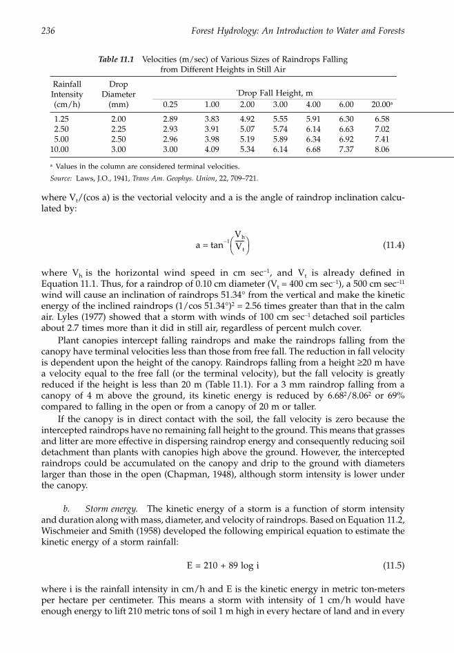
236 Forest Hydrology: An Introduction to Water and Forests
where V
t
/(cos a) is the vectorial velocity and a is the angle of raindrop inclination calcu-lated by:
(11.4)
where V
h
is the horizontal wind speed in cm sec
-
1
, and V
t
is already defined inEquation 11.1. Thus, for a raindrop of 0.10 cm diameter (V
t
= 400 cm sec
-
1
), a 500 cm sec
–11
wind will cause an inclination of raindrops 51.34
∞
from the vertical and make the kineticenergy of the inclined raindrops (1/cos 51.34
∞
)
2
= 2.56 times greater than that in the calmair. Lyles (1977) showed that a storm with winds of 100 cm sec
-
1
detached soil particlesabout 2.7 times more than it did in still air, regardless of percent mulch cover.
Plant canopies intercept falling raindrops and make the raindrops falling from thecanopy have terminal velocities less than those from free fall. The reduction in fall velocityis dependent upon the height of the canopy. Raindrops falling from a height
≥
20 m havea velocity equal to the free fall (or the terminal velocity), but the fall velocity is greatlyreduced if the height is less than 20 m (Table 11.1). For a 3 mm raindrop falling from acanopy of 4 m above the ground, its kinetic energy is reduced by 6.68
2
/8.06
2
or 69%compared to falling in the open or from a canopy of 20 m or taller.
If the canopy is in direct contact with the soil, the fall velocity is zero because theintercepted raindrops have no remaining fall height to the ground. This means that grassesand litter are more effective in dispersing raindrop energy and consequently reducing soildetachment than plants with canopies high above the ground. However, the interceptedraindrops could be accumulated on the canopy and drip to the ground with diameterslarger than those in the open (Chapman, 1948), although storm intensity is lower underthe canopy.
b. Storm energy.
The kinetic energy of a storm is a function of storm intensityand duration along with mass, diameter, and velocity of raindrops. Based on Equation 11.2,Wischmeier and Smith (1958) developed the following empirical equation to estimate thekinetic energy of a storm rainfall:
E = 210 + 89 log i (11.5)
where i is the rainfall intensity in cm/h and E is the kinetic energy in metric ton-metersper hectare per centimeter. This means a storm with intensity of 1 cm/h would haveenough energy to lift 210 metric tons of soil 1 m high in every hectare of land and in every
Table 11.1
Velocities (m/sec) of Various Sizes of Raindrops Falling
from Different Heights in Still Air
Rainfall Intensity(cm/h)
Drop Diameter
(mm)
˙Drop Fall Height, m0.25 1.00 2.00 3.00 4.00 6.00 20.00
a
1.25 2.00 2.89 3.83 4.92 5.55 5.91 6.30 6.582.50 2.25 2.93 3.91 5.07 5.74 6.14 6.63 7.025.00 2.50 2.96 3.98 5.19 5.89 6.34 6.92 7.41
10.00 3.00 3.00 4.09 5.34 6.14 6.68 7.37 8.06
a
Values in the column are considered terminal velocities.
Source:
Laws, J.O., 1941,
Trans Am. Geophys. Union
, 22, 709–721.
a = tan 1–Vh
Vt------
Ë ¯Ê �
1363_C11_fm Page 236 Wednesday, December 4, 2002 7:44 AM
Chapter eleven: Forests and stream sediment 237
1 cm of rainfall. If this storm lasts only 30 minutes and the total rainfall is 0.50 cm (stormintensity still = 1 cm/h), then the E value is equivalent to 105 metric tons of soil 1 m highper hectare. Equation 11.5 applies to i
£
7.6 cm/h. For i > 7.6 cm/h, E = 289 t-m/ha-cmof rain. Other rainfall indices that relate kinetic energy to rainfall intensity or amount canbe obtained from McGregor and Mutchler (1977), Morgan (1986), and Lal and Elliot (1994).
Estimating total kinetic energy of a storm requires the sequential progress of rainfalldepth vs. time, such as observations on a recording raingage chart. The storm is thenbroken down into segments of uniform intensity. Calculate the kinetic energy of eachsegment by the product of Equation 11.5 and the total rainfall in the segment, and finallysum the kinetic energy of all segments to yield the total kinetic energy (see part II). Inforested areas, total kinetic energy needs to be modified by considering percent forestcanopy coverage and the height of the canopy in this form:
E
e
= E (11.6)
where E
e
= the effective kinetic energy of rainfall; E = the kinetic energy in the open,calculated by Equation 11.5; M = rainfall mass; v = raindrop velocity; and F = fraction ofcanopy coverage. Subscripts th and o, respectively, refer to throughfall and gross rainfallin the open. If the forest is taller than 20 m, then (V
th
/V
o
)
2
= 1.0 and is omitted from theequation.
c. Freezing water.
Water expands as it freezes. The volume at
-
10
∞
C is 0.187%greater than at 4
∞
C, the smallest volume of water at any thermal condition. Such volumeexpansion exerts a pressure equivalent to about 146 kg cm
-
2
. Thus, alternate freezing andthawing cause disintegration of rock, mineral, and soil aggregates.
d. Soil resistance.
Soil particles are bound to hold together due to cohesion, inter-nal friction, and organic colloids. The force that holds particles together is often referredto as shear strength, and the ability of soil structural units to withstand the forces ofraindrop impact and surface flow is called detachability. Generally, soil detachabilitydecreases with increasing organic-matter content and infiltration rate, and increases withincreasing particle size up to about 0.5 mm (Figure 11.1). Organic matter stabilizes soilstructure by binding soil particles together. It forms an organo-mineral complex that canresist microbial degradation in soil for many years. The complex determines the durationand effectiveness in stabilizing soil particles (Barry et al., 1991).
For a given volume of soil, the total surface area for small particles is much greaterthan for large particles, which causes an increase in particle contact and cohesive forceand consequently a greater resistance to detachment. However, the weight of particlesovercomes the surface attraction if the size is larger than about 0.5 mm. It then requiresa great force to move the particles as the size increases. An interrill-erosion study con-ducted on 18 soils with a wide range of textures showed that the silt and silt loam soilswere most erodible, the high-clay soils were least erodible, and the loam and sandy loamsoils were intermediate (Meyer and Harmon, 1984).
Shear strength is commonly determined by a series of (three or four) triaxial compres-sion tests at different confining pressures carried to failure stresses in the laboratory andis defined by the Mohr-Coulomb equation (Parker et al., 1980):
t
c
= C +
s
n
tan
f
(11.7)
1 F–( ) FMth
Mo---------
Ë ¯Ê �
Vth
Vo-------
Ë ¯Ê �
2
+
1363_C11_fm Page 237 Wednesday, December 4, 2002 7:44 AM
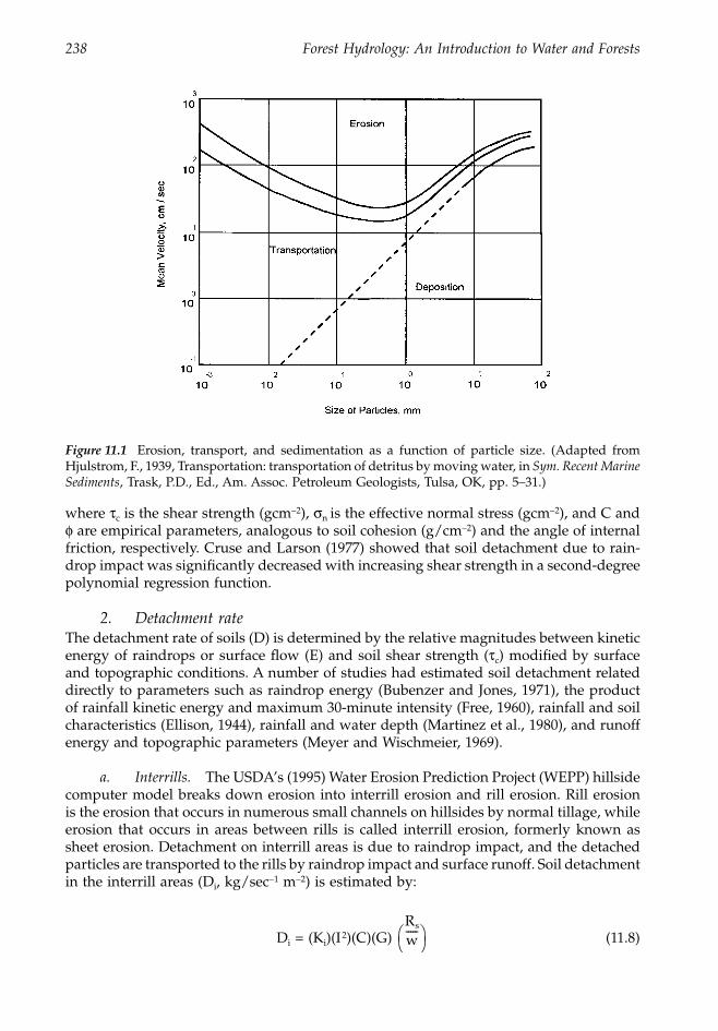
238 Forest Hydrology: An Introduction to Water and Forests
where
t
c
is the shear strength (gcm
-
2
),
s
n
is the effective normal stress (gcm
-
2
), and C and
f
are empirical parameters, analogous to soil cohesion (g/cm
-
2
) and the angle of internalfriction, respectively. Cruse and Larson (1977) showed that soil detachment due to rain-drop impact was significantly decreased with increasing shear strength in a second-degreepolynomial regression function.
2. Detachment rate
The detachment rate of soils (D) is determined by the relative magnitudes between kineticenergy of raindrops or surface flow (E) and soil shear strength (
t
c
) modified by surfaceand topographic conditions. A number of studies had estimated soil detachment relateddirectly to parameters such as raindrop energy (Bubenzer and Jones, 1971), the productof rainfall kinetic energy and maximum 30-minute intensity (Free, 1960), rainfall and soilcharacteristics (Ellison, 1944), rainfall and water depth (Martinez et al., 1980), and runoffenergy and topographic parameters (Meyer and Wischmeier, 1969).
a. Interrills.
The USDA’s (1995) Water Erosion Prediction Project (WEPP) hillsidecomputer model breaks down erosion into interrill erosion and rill erosion. Rill erosionis the erosion that occurs in numerous small channels on hillsides by normal tillage, whileerosion that occurs in areas between rills is called interrill erosion, formerly known assheet erosion. Detachment on interrill areas is due to raindrop impact, and the detachedparticles are transported to the rills by raindrop impact and surface runoff. Soil detachmentin the interrill areas (D
i
, kg/sec
-
1
m
-
2
) is estimated by:
D
i
= (K
i
)(I
2
)(C)(G) (11.8)
Figure 11.1
Erosion, transport, and sedimentation as a function of particle size. (Adapted fromHjulstrom, F., 1939, Transportation: transportation of detritus by moving water, in
Sym. Recent MarineSediments
, Trask, P.D., Ed., Am. Assoc. Petroleum Geologists, Tulsa, OK, pp. 5–31.)
Rs
w-----
Ë ¯Ê �
1363_C11_fm Page 238 Wednesday, December 4, 2002 7:44 AM

Chapter eleven: Forests and stream sediment 239
where K
i
is interrill erodibility (kg-sec m
-
4
), I is effective rainfall intensity (m sec
-
1
), C isthe effect of canopy on interrill erosion (0–1), G is the effect of ground cover (0–1), R
s
isthe spacing of rills (m), and w is the computed rill width (m). Values of K
i
for croplandsoils with 30% or more of sand are estimated by the equation:
K
i
= 272800 + 19210000 (vfs) (11.9)
and use the following equation if the sand is less than 30%:
K
i
= 605400 – 5513000 (clay) (11.10)
where vfs and clay are the fraction of very fine sand and clay in the surface soil, respec-tively. The enormous coefficients in Equations 11.9 and 11.10 are due to the large unit ofrainfall intensity used in the model. The estimated values from these two equations arethen adjusted to account for various site effects, including canopy cover, ground cover,roots, slope, freeze-thaw cycles, and sealing and crusting. Meyer and Harmon (1984)showed that interrill soil erodibilities were negatively correlated with percent dispersedclay (<2
m
m), percent water content at 1500 kPa, exchangeable calcium, sum of exchange-able bases, and cation exchange capacity with correlation coefficients ranging from 0.80to 0.86.
b. Rills.
The difference between flow shear stress
t
and critical shear strength ofsoil
t
c
, all in force per unit area or Newton m
-
2
(1 N m
-
2
= 1 kg m
-
1
sec
-
2
= 1 pascal), canbe used to estimate soil detachment in the rills, or:
D
c
= K
r
(
t
–
t
c
) (11.11)
where D
c
is detachment capacity by rill flow (kg sec
-
1
m
-
2
) and K
r
is rill erodibility(sec m
–1
). In other words, there is no rill detachment when
t is less than tc. For crop soilswith 30% or more of sand, the erodibility and the critical shear strength are estimated by:
Kr = 0.00197 + 0.030 (vfs) + 0.03863 e-184 (OM) (11.12)
tc = 2.67 + 6.5 (clay) – 5.8 (vfs) (11.13)
where OM is percent organic matter in the surface soil. For crop soils with less than30% sand,
Kr = 0.0069 + 0.134 e-20 (clay) (11.14)
tc = 3.5 (11.15)
Like Ki, the calculated Kr needs to be adjusted for other soil factors. The flow shear stresst is calculated by:
t = g Rs (11.16)
where g is the specific weight of water (Newton/m3 or kg m-2 sec-2), R is the hydraulicradius of rill or substituted by depth of flow (m), and s the hydraulic gradient of rill flow.
1363_C11_fm Page 239 Wednesday, December 4, 2002 7:44 AM
240 Forest Hydrology: An Introduction to Water and Forests
These equations employ the concept that soil detachment on interrill areas is primarilyinduced by rainfall energy and ignore the minor impact from overland flow. Rainfallintensity is rarely constant during a storm, which causes the soil detachment rate to be atime-dependent function. Unfortunately, the time-dependence effect of changing soildetachment has been lumped with the rainfall parameter in most studies (Foster andMeyer, 1975). On the other hand, detachment in rill areas is primarily induced by concen-trated flow and ignores the minor impact from rainfall impact. Once particles are detachedfrom soil mass, the energy required to transport the sediment is much smaller.
B. Transport
For detached particles to become stream sediment, they require agents to carry them onto new locations and eventually to stream channels. Both rainfall and runoff can transportsoil particles.
1. Rainfall transportTransport of soil particles by rainfall is due to splash action, and the splash capacity isa function of rainfall amount and intensity, slope gradient, soil characteristics, windspeed, and microrelief. As a rule of thumb, the percentage of total splashed soil thatmoves downslope equals the percent slope plus 50 (Ekern, 1953). However, the majorimpact of raindrop energy is for soil detachment, not for transport, in interrill areas. Thedetached and splashed particles are then transported primarily by broad shallow surfaceflow to rills (Nearing et al., 1994). There, soil particles from rill and interrill areas arejoined together and transported to stream channels by concentrated flow (Young andWiersma, 1973).
2. Runoff transportThe maximum amount of sediment that an overland flow can carry, often referred to astransport capacity, depends on its energy level as determined by flow velocity and mass,slope gradient, hydraulic radius, surface roughness, and particle transportability. A tur-bulent flow is more erosive and carries more particles than a laminar flow, while pondingof the flow produces rapid deposition. Since the velocity of overland flow increases withdepth (Equation 10.29), the transport capacity is greater and transport distance is longerfor deep flows. Thus, a reduction in overland flow or discharge, an increase in cross-sectional area, or a change in slope will cause a decrease in transport capacity. As a result,the heavier, larger, and round particles deposit first, while the smaller, lighter, and platyparticles remain in suspension. Thus, particles of larger sizes are deposited upstream andsmaller sizes downstream.
Silted flows are more erosive than clean ones. Abrasion and crushing of particlesagainst one another take place as they are transported in the flow. This makes largeparticles wear away into smaller ones and they are carried farther downstream. In relativeterms, shale and sandstone are more easily crushed than limestone and dolomite, whilegranite and quartz are less easily crushed (Gottschalk, 1964).
In field investigations, sediment-carrying capacity of flowing water was found to beapproximately proportional to the fifth power of flow velocity (Laursen, 1958), to the 1.5thpower of bottom shear stress (Foster and Meyer, 1972), or to stream power, the productof bottom shear stress and flow velocity (Yang, 1972). A more comprehensive equation toestimate total sediment transport capacity (Tc, in mass/width or kg/sec · m) of overlandflow for a storm is given by Foster (1982):
Tc = 138 Q q S1.55 Ct (11.17)
1363_C11_fm Page 240 Wednesday, December 4, 2002 7:44 AM
Chapter eleven: Forests and stream sediment 241
where Q = total discharge/width (m3/sec · m), q = peak discharge/width (m3/sec · m),S = sine of slope angle, and Ct = a factor reflecting the direct influence of soil cover onthe flow’s hydraulic forces. The Ct value is 1.0 (maximum) for a bare ground and 0.2for an 8% slope with light mulch. The coefficient and exponent, depending on particlesize, in Equation 11.17 represent conditions typical of most aggregated soils. Sincedischarge is estimated by the product of flow velocity, width, and depth, Equation 11.17can be substituted by:
Tc = 138 (V)(q)(d)(S1.55)(Ct) (11.18)
where V is flow velocity in m/sec, and d is flow depth in m.
C. Deposition
The deposition of moving particles depends on the relative magnitudes of transportcapacity and sediment load (determined by soil detachment). If sediment load is less thantransport capacity, then the sediment load moves downslope. If sediment load exceedstransport capacity, then deposition occurs. This can be expressed by:
Dp = Cd (Tc – D) (11.19)
where Dp = deposition rate in kg/sec · m, Tc = transport capacity in kg/sec · m, D = sedimentload, kg/sec · m, and Cd = the first-order reaction coefficient for deposition in per unitwidth. A small value of Cd means a greater distance in particle transport and consequentlyless deposition. The value decreases with a decrease in particle size and fall velocity, butincreases as discharge increases. Foster (1982) gave the following equation to estimate Cd
for deposition by overland flow:
Cd = 0.5 (11.20)
where Vf = fall velocity in m/sec, and Q = discharge in m3/sec · m. The fall velocity Vf,in cm/sec, can be estimated by Stokes’s law:
Vf = (g)(r2) (11.21)
where r is the radius of particle in cm, g is the acceleration due to gravity, dp is the densityof the particle, d is the density of the liquid, and h is the absolute (dynamic) viscosity ofthe liquid. The equation describes that the fall velocity of particles of the same density ina given liquid will increase with the square of the particle radius. For silts withr = 0.0005 cm, dp = 1.2 g/cm3, and h at 20∞C = 1.818 (10-4) g/cm · sec, the fall velocity willbe 0.09 cm/sec in a liquid water. If the silts are transported in an overland flow of 1.0 cmdeep and 0.5 m/sec velocity, then those particles at the water surface would be carried inthe flow for about 11 seconds and be deposited 5.5 m downslope.
For a typical midwestern soil, the reaction coefficient Cd for clay (2 µm), silt (10 µm),and sand (200 µm) is about 0.009/m, 0.074/m, and 22.0/m, respectively (Foster, 1982).
V f
Q------
Ë ¯Ê �
29---
Ë ¯Ê �
dp d–h
---------------Ë ¯Ê �
1363_C11_fm Page 241 Wednesday, December 4, 2002 7:44 AM
242 Forest Hydrology: An Introduction to Water and Forests
II. Watershed gross erosionSoil erosion in a watershed can be categorized into six major sources: interrills, rills,ephemeral gullies, gullies, channels, and landslides. The sum of soil erosion from thesesix sources is called watershed gross erosion. Only a fraction of the watershed gross erosionwill reach stream channels during a storm and the rest is trapped within the watershedsubject to actions of other storm events.
A. Interrill and rill erosion
Surface runoff often concentrates in numerous small downslope channels that are uni-formly spread across the field. Such small channels can be removed by normal tillagepractices, and the soil loss that occurs along these small channels is termed rill erosion.Erosion in areas between rills is called interrill erosion. Severe rill erosion can exceed448 t/ha/year (Foster, 1986), while interrill erosion rates as high as 45 t/ha/year havebeen measured (Meyer, 1981).
Empirical, factor-based, and physical models have been developed for estimatinginterrill and rill erosion. Most physical models treat interrill and rill erosion in two differentprocesses, while the empirical and factor-based models combine them in a single estimate.
1. EmpiricalThe empirical approach relates observed erosion data to environmental factors throughstatistical analysis. Generally, it is easier to develop models for estimating soil losses oflong-term average than for single storms, and for general areas than for specific areas.Since those models are not derived theoretically, they are applicable only in regions wherethe studies were conducted and under similar environmental conditions. Thus, the reli-ability of estimates depends on the representativeness of the data used in the modeldevelopment and the suitability of area for model applications.
The first model to estimate soil loss for hillslopes was developed by Zingg (1940) asa function of two topographic parameters:
A = ¶(tan1.4 q L0.6) (11.22)
where q is the angle of slope gradient and L is slope length. This pioneer study triggeredother studies to relate soil loss with environmental factors, such as climatic conditions,soils, and vegetation cover. Later, using soil loss data collected from 40,000 plot-yearsunder a wide range of rainfall conditions, Musgrave (1947) gave a prediction model thatused topographic as well as climatic, edaphic, and cover factors:
A = K C (S1.35) (L 0.35) [(P0.5)1.75] b (11.23)
where A = soil loss (acre-in. or ha-cm), K = inherent soil erodibility (in. or cm), C = coverfactor, L = slope length (ft or m), S = land slope (%), P0.5 = maximum 30-minute rainfallwith a 2-year return period (in. or cm), and b = a conversion factor if the equation isexpressed in metric units instead of the original British units. The Musgrave equation wasused by the Soil Conservation Service for about 10 years and was the pioneer version ofthe universal soil-loss equation.
2. Factor-basedA factor-based model contains a number of factors, such as rainfall, soil, topography,vegetation, and management, that may affect soil losses significantly. The effect of each
1363_C11_fm Page 242 Wednesday, December 4, 2002 7:44 AM

Chapter eleven: Forests and stream sediment 243
factor on soil loss is separately quantified, based on either observed data or theoreticalconsiderations. Each factor may quantify one or more erosion processes and their inter-actions. Finally, all factors are multiplied together to give the estimate. Although factor-based models are also largely based on data experience, the final equations are not obtainedthrough statistical analyses. It is semiempirical and still has certain limitations. The mostpopular ones are the universal soil-loss equation (Wischmeier, 1975) and its modifiedversion (USDA, 1995).
a. Universal soil loss equation (USLE). The USLE was originally developed by theAgricultural Research Service (ARS) and SCS in the 1950s to estimate average annualinterrill and rill erosion from agricultural lands for areas east of the Rocky Mountains. Itwas extended to cover the entire conterminous U.S. in the middle of the 1970s. The USLEhas been a very valuable and successful tool for land management and planning for nearly50 years.
The USLE estimates soil loss (A) as the product of rainfall factor (R) and soil factor(K) with modifications of slope steepness factor (S), slope length factor (L), conservationpractice factor (P), and cover and management factor (C):
A = RKLSCP (11.24)
where A is the estimated soil loss, is in ton/acre/year (1 ton/acre/year = 0.446 t/ha/year)and R is the rainfall factor is the energy term to generate soil erosion. For a single storm,the erosive energy is indexed by the product of storm kinetic energy E in ft-ton/acre-in.(1 ft-ton/acre-in. = 0.268 t/ha-cm) and the maximum 30-minute storm intensity (I30) inin./h (or cm/h) divided by 100. For a duration corresponding to A, R is calculated by:
(11.25)
where n refers to the total number of years, m refers to storms in each year, and E is stormkinetic energy in British unit (ft-ton/acre-in.) calculated by following equation:
E = 916 + 331 log i, for i £ 3 inches/hr (11.26)
where i is in in./h. For i > 3 in./h, E = 1074 foot-tons per acre per inch of rainfall. Equation11.26 is Equation 11.5 in British unit. The conversion of the universal soil loss equationfrom British units to SI metric units was given by Foster et al. (1981) in great detail.
The calculation of R for a single storm requires rainfall intensity data (depth vs. time)such as that shown in a recording raingage chart. First, a storm is broken down intosegments of uniform intensity. Calculate the E value for each segment first per in. of rainfallusing Equation 11.26 (or per cm of rainfall using Equation 11.5), and then multiply theE/in. of rainfall (or E/cm of rainfall) by the total rainfall in inches (or in cm) in the segmentto obtain the total E value for that segment. Sum the total kinetic energy of each segmentto yield total E value for the entire storm. Finally, multiply the total storm energy E withthe maximum 30-minute storm intensity in in./h (or in cm/h) and divide the product by100 to yield the R factor for the storm. The calculation procedure is given in Table 11.2.Average annual R-values for the conterminous U.S., in hundreds of ft-ton-in./acre-h-year,are given in Figure 11.2 (Wischmeier and Smith, 1978). To convert R in the British unitsto metric units in hundreds of t-m-cm/ha-h-year or to SI units in MJ-mm/ha-h-year,multiply by the factor 1.735 or 17.02, respectively.
R EI30( )
m
Â
n
 / 100 n( )=
1363_C11_fm Page 243 Wednesday, December 4, 2002 7:44 AM
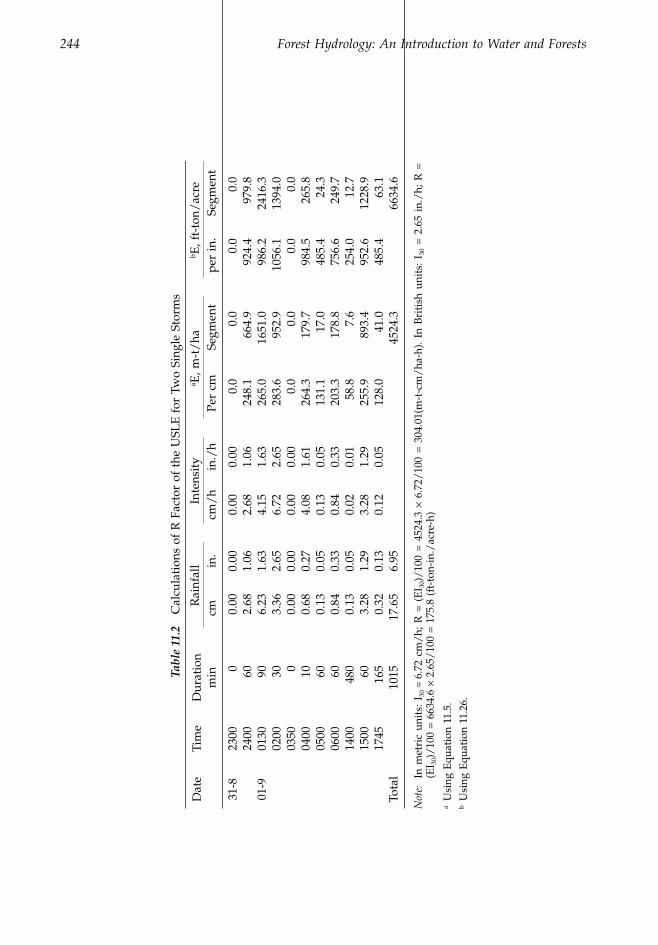
244 Forest Hydrology: An Introduction to Water and Forests
Tabl
e 11
.2C
alcu
lati
ons
of R
Fac
tor
of t
he U
SLE
for
Tw
o Si
ngle
Sto
rms
Dat
eTi
me
Dur
atio
nm
in
Rai
nfal
lIn
tens
ity
a E, m
-t/
hab E
, ft-
ton/
acre
cmin
.cm
/h
in./
h Pe
r cm
Se
gmen
t pe
r in
.Se
gmen
t
31-8
2300
00.
000.
000.
000.
000.
00.
00.
00.
024
0060
2.68
1.06
2.68
1.06
248.
166
4.9
924.
497
9.8
01-9
0130
906.
231.
634.
151.
6326
5.0
1651
.098
6.2
2416
.302
0030
3.36
2.65
6.72
2.65
283.
695
2.9
1056
.113
94.0
0350
00.
000.
000.
000.
000.
00.
00.
00.
004
0010
0.68
0.27
4.08
1.61
264.
317
9.7
984.
526
5.8
0500
600.
130.
050.
130.
0513
1.1
17.0
485.
424
.306
0060
0.84
0.33
0.84
0.33
203.
317
8.8
756.
624
9.7
1400
480
0.13
0.05
0.02
0.01
58.8
7.6
254.
012
.715
0060
3.28
1.29
3.28
1.29
255.
989
3.4
952.
612
28.9
1745
165
0.32
0.13
0.12
0.05
128.
041
.048
5.4
63.1
Tota
l10
1517
.65
6.95
4524
.366
34.6
Not
e:
In m
etri
c un
its:
I30
= 6
.72
cm/
h; R
= (
EI 3
0)/
100
= 4
524.
3 ¥
6.72
/10
0 =
304
.01(
m-t
-cm
/ha
-h).
In B
riti
sh u
nits
: I 3
0 =
2.6
5 in
./h;
R =
(EI 3
0)/
100
= 6
634.
6 ¥
2.65
/10
0 =
175
.8 (
ft-t
on-i
n./
acre
-h)
aU
sing
Equ
atio
n 11
.5.
bU
sing
Equ
atio
n 11
.26.
1363_C11_fm Page 244 Wednesday, December 4, 2002 7:44 AM
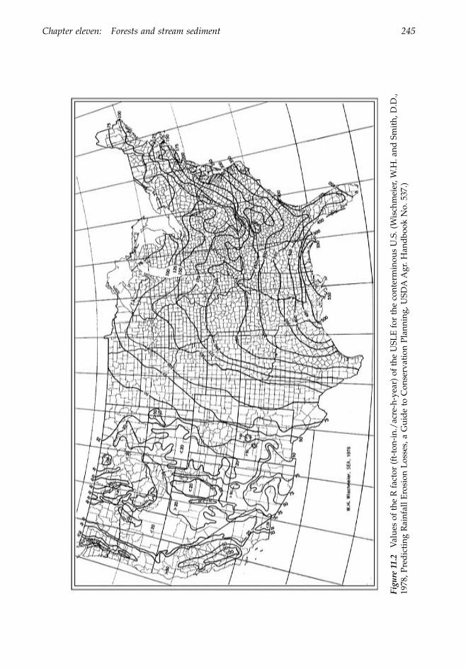
Chapter eleven: Forests and stream sediment 245
Figu
re 1
1.2
Val
ues
of t
he R
fac
tor
(ft-
ton-
in./
acre
-h-y
ear)
of
the
USL
E f
or t
he c
onte
rmin
ous
U.S
. (W
isch
mei
er, W
.H. a
nd S
mit
h, D
.D.,
1978
, Pre
dic
ting
Rai
nfal
l Ero
sion
Los
ses,
a G
uid
e to
Con
serv
atio
n Pl
anni
ng, U
SDA
Agr
. Han
dbo
ok N
o. 5
37.)
1363_C11_fm Page 245 Wednesday, December 4, 2002 7:44 AM
246 Forest Hydrology: An Introduction to Water and Forests
The calculation of R values illustrated above is laborious and requires rainfall intensitydata that may not be available for the location in question. Many efforts have been madein different parts of the world to estimate the R values based on monthly or annualprecipitation data (Roose, 1977; Arnoldus, 1980; Simanton and Renard, 1982; Lo et al.,1985). Although reasonable estimates can be obtained by those substitute methods, theirapplication is limited to areas where they were developed. Perhaps the largest applicationsin area are the models Renard and Freimund (1994) developed in the U.S. Based on 132stations throughout the U.S. (except for locations in western Washington, western Oregon,and northern California), one of the models appeared as:
R = 0.1922 (Pt)1.61 (11.27)
where R is in 100s of t-m-cm/ha-year-h, and Pt is mean annual precipitation in cm. Theequation seems to overestimate R-values in the North and the Northeast, and underesti-mate those in the other regions.
K, the soil erodibility factor, describes both soil detachability and transportability dueto various soil properties such as texture, structure, organic matter, density, compaction,and biological characteristics. These properties in turn affect soil infiltration and percola-tion, water-holding capacity, and surface runoff, parameters of the utmost importance tosoil-erosion processes. The K value in Equation 11.24 is the average soil loss per unit valueof RLSCP, or:
K = A/(RLSCP) (11.28)
Assuming the land is bare, 9% slope, 22.13 m (72.6 ft) long, continuously plowed upand down the hill, and undergoing no conservation practices, all the LSCP values areequal to 1 and the equation becomes K = A/R. Field observations for a wide range of soiltypes showed that percent silt and very fine sand, percent of sand, percent of organicmatter, soil structure, and permeability are most significant to the variation of K. The Kvalue for a particular soil can be obtained from the NRCS’ county soil survey report. Ifthe information for the five soil properties is available, it can be read directly fromFigure 11.3, or solved by the following equation:
100 K = 2.1M1.14 (10–4)(12-a) + 3.25 (b-2) + 2.5 (c-3) (11.29)
where M = (silt + very fine sand %) (100 - clay), a = percent organic matter, b = thesoil structure code used in soil classification, and c = the profile permeability class.Equation 11.29 and Figure 11.3 give K in British units (ton/ac/EI), or 1 K in British unit= 0.342 K in metric unit (t/ha/EI in metric units). Values of K typically range from about0.10 to 0.45 in British units. Soils with high clay or sand content have lower K values,while soils with high content of silt have higher K values.
The LS factor in Equation 11.24, describes the effects of topography: as the slope lengthincreases, runoff per unit area decreases, but the accumulation (concentration) of runoffincreases, resulting in greater soil loss per unit area. On the other hand, steep slopes causelower infiltration rate, greater surface runoff, higher flow velocity, longer splash distance,and more soil detachment and transport. The relationship between soil loss and slopelength (l) has generally been described with the exponential function, soil loss = c (l)a
where soil loss is in mass or mass/area, l has units of distance, and c and a are constants.
1363_C11_fm Page 246 Wednesday, December 4, 2002 7:44 AM
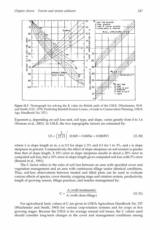
Chapter eleven: Forests and stream sediment 247
Exponent a, depending on soil loss unit, soil type, and slope, varies greatly from 0 to 1.6(Truman et al., 2001). In USLE, the two topographic factors are estimated by:
LS = (0.065 + 0.0454s + 0.0065S2) (11.30)
where l is slope length in m, a is 0.5 for slope ≥ 5% and 0.3 for 1 to 3%, and s is slopesteepness in percent. Comparatively, the effect of slope steepness on soil erosion is greaterthan that of slope length. A 10% error in slope steepness results in about a 20% error incomputed soil loss, but a 10% error in slope length gives computed soil loss with 5% error(Renard et al., 1991).
The C factor refers to the ratio of soil loss between an area with specified cover andvegetation management and an area with continuous tillage under identical conditions.Thus, soil-loss observations between treated and tilled plots can be used to evaluatevarious effects of species, cover density, cropping stage and rotation system, productivity,length of growing season, tillage practices, and residue management by:
C = (11.31)
For agricultural land, values of C are given in USDA Agriculture Handbook No. 537(Wischmeier and Smith, 1965) for various crop-rotation systems and for crops at fivegrowing stages. Because the USLE is for average annual soil losses, the C values usedshould consider long-term changes in the cover and management conditions among
Figure 11.3 Nomograph for solving the K value (in British unit) of the USLE. (Wischmeier, W.H.and Smith, D.D., 1978, Predicting Rainfall Erosion Losses, a Guide to Conservation Planning, USDAAgr. Handbook No. 537.)
l22.13-------------
Ë ¯Ê �
a
A with treatments( )A with clean tillage( )--------------------------------------------------------
1363_C11_fm Page 247 Wednesday, December 4, 2002 7:44 AM
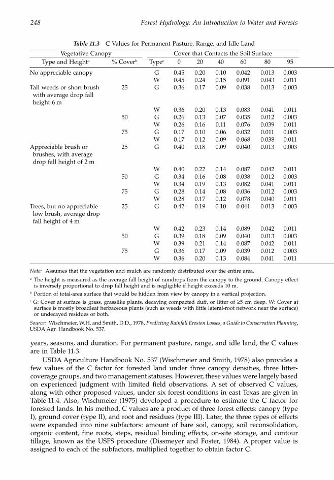
248 Forest Hydrology: An Introduction to Water and Forests
years, seasons, and duration. For permanent pasture, range, and idle land, the C valuesare in Table 11.3.
USDA Agriculture Handbook No. 537 (Wischmeier and Smith, 1978) also provides afew values of the C factor for forested land under three canopy densities, three litter-coverage groups, and two management statuses. However, these values were largely basedon experienced judgment with limited field observations. A set of observed C values,along with other proposed values, under six forest conditions in east Texas are given inTable 11.4. Also, Wischmeier (1975) developed a procedure to estimate the C factor forforested lands. In his method, C values are a product of three forest effects: canopy (typeI), ground cover (type II), and root and residues (type III). Later, the three types of effectswere expanded into nine subfactors: amount of bare soil, canopy, soil reconsolidation,organic content, fine roots, steps, residual binding effects, on-site storage, and contourtillage, known as the USFS procedure (Dissmeyer and Foster, 1984). A proper value isassigned to each of the subfactors, multiplied together to obtain factor C.
Table 11.3 C Values for Permanent Pasture, Range, and Idle Land
Vegetative Canopy Cover that Contacts the Soil SurfaceType and Heighta % Coverb Typec 0 20 40 60 80 95
No appreciable canopy G 0.45 0.20 0.10 0.042 0.013 0.003W 0.45 0.24 0.15 0.091 0.043 0.011
Tall weeds or short brush with average drop fall height 6 m
25 G 0.36 0.17 0.09 0.038 0.013 0.003
W 0.36 0.20 0.13 0.083 0.041 0.01150 G 0.26 0.13 0.07 0.035 0.012 0.003
W 0.26 0.16 0.11 0.076 0.039 0.01175 G 0.17 0.10 0.06 0.032 0.011 0.003
W 0.17 0.12 0.09 0.068 0.038 0.011Appreciable brush or brushes, with average drop fall height of 2 m
25 G 0.40 0.18 0.09 0.040 0.013 0.003
W 0.40 0.22 0.14 0.087 0.042 0.01150 G 0.34 0.16 0.08 0.038 0.012 0.003
W 0.34 0.19 0.13 0.082 0.041 0.01175 G 0.28 0.14 0.08 0.036 0.012 0.003
W 0.28 0.17 0.12 0.078 0.040 0.011Trees, but no appreciable low brush, average drop fall height of 4 m
25 G 0.42 0.19 0.10 0.041 0.013 0.003
W 0.42 0.23 0.14 0.089 0.042 0.01150 G 0.39 0.18 0.09 0.040 0.013 0.003
W 0.39 0.21 0.14 0.087 0.042 0.01175 G 0.36 0.17 0.09 0.039 0.012 0.003
W 0.36 0.20 0.13 0.084 0.041 0.011
Note: Assumes that the vegetation and mulch are randomly distributed over the entire area.a The height is measured as the average fall height of raindrops from the canopy to the ground. Canopy effect
is inversely proportional to drop fall height and is negligible if height exceeds 10 m.b Portion of total-area surface that would be hidden from view by canopy in a vertical projection.c G: Cover at surface is grass, grasslike plants, decaying compacted duff, or litter of ≥5 cm deep. W: Cover at
surface is mostly broadleaf herbaceous plants (such as weeds with little lateral-root network near the surface)or undecayed residues or both.
Source: Wischmeier, W.H. and Smith, D.D., 1978, Predicting Rainfall Erosion Losses, a Guide to Conservation Planning,USDA Agr. Handbook No. 537.
1363_C11_fm Page 248 Wednesday, December 4, 2002 7:44 AM
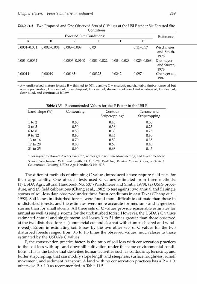
Chapter eleven: Forests and stream sediment 249
The different methods of obtaining C values introduced above require field tests fortheir applicability. One of such tests used C values estimated from three methods:(1) USDA Agricultural Handbook No. 537 (Wischmeier and Smith, 1978), (2) USFS proce-dure, and (3) field calibrations (Chang et al., 1982) to test against two annual and 51 singlestorms of soil-loss data observed under three forest conditions in east Texas (Chang et al.,1992). Soil losses in disturbed forests were found more difficult to estimate than those inundisturbed forests, and the estimates were more accurate for medium- and large-sizedstorms than for small storms. All three sets of C values provide reasonable estimates forannual as well as single storms for the undisturbed forest. However, the USDA’s C valuesestimated annual and single storm soil losses 3 to 51 times greater than those observedat the two disturbed forests (commercial cut and clearcut with stumps sheared and wind-rowed). Errors in estimating soil losses by the two other sets of C values for the twodisturbed forests ranged from 0.5 to 1.5 times the observed values, much closer to thoseestimated by the USDA’s C values.
P, the conservation practice factor, is the ratio of soil loss with conservation practicesto the soil loss with up- and downhill cultivation under the same environmental condi-tions. This is the factor that describes human activities such as contouring, terracing, andbuffer stripcroping, that can modify slope length and steepness, surface roughness, runoffmovement, and sediment transport. A land with no conservation practices has a P = 1.0,otherwise P < 1.0 as recommended in Table 11.5.
Table 11.4 Two Proposed and One Observed Sets of C Values of the USLE under Six Forested Site Conditions
Forested Site Conditionsa ReferenceA B C D E F
0.0001–0.001 0.002–0.004 0.003–0.009 0.03 0.11–0.17 Wischmeier and Smith, 1978
0.001–0.0034 0.0003–0.0100 0.001–0.022 0.004–0.028 0.023–0.068 Dissmeyer and Stump, 1978
0.00014 0.00019 0.00165 0.00325 0.0242 0.097 Chang et al., 1982
a A = undisturbed mature forests; B = thinned to 50% density; C = clearcut, merchantable timber removed butno site preparation; D = clearcut, roller chopped; E = clearcut, sheared, root raked and windrowed; F = clearcut,clear tilled, and continuous fallow.
Table 11.5 Recommended Values for the P Factor in the USLE
Land slope (%) Contouring Contour Stripcroppinga
Terrace and Stripcropping
1 to 2 0.60 0.45 0.303 to 5 0.50 0.38 0.256 to 8 0.50 0.38 0.259 to 12 0.60 0.45 0.3013 to 16 0.70 0.52 0.3517 to 20 0.80 0.60 0.4021 to 25 0.90 0.68 0.45
a For 4-year rotation of 2 years row crop, winter grain with meadow seeding, and 1-year meadow.
Source: Wischmeier, W.H. and Smith, D.D., 1978, Predicting Rainfall Erosion Losses, a Guide toConservation Planning, USDA Agr. Handbook No. 537.
1363_C11_fm Page 249 Wednesday, December 4, 2002 7:44 AM
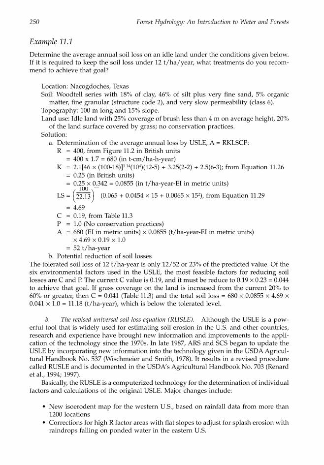
250 Forest Hydrology: An Introduction to Water and Forests
Example 11.1
Determine the average annual soil loss on an idle land under the conditions given below.If it is required to keep the soil loss under 12 t/ha/year, what treatments do you recom-mend to achieve that goal?
Location: Nacogdoches, TexasSoil: Woodtell series with 18% of clay, 46% of silt plus very fine sand, 5% organic
matter, fine granular (structure code 2), and very slow permeability (class 6).Topography: 100 m long and 15% slope.Land use: Idle land with 25% coverage of brush less than 4 m on average height, 20%
of the land surface covered by grass; no conservation practices.Solution:
a. Determination of the average annual loss by USLE, A = RKLSCP:R = 400, from Figure 11.2 in British units = 400 x 1.7 = 680 (in t-cm/ha-h-year)K = 2.1[46 ¥ (100-18)]1.14(104)(12-5) + 3.25(2-2) + 2.5(6-3); from Equation 11.26
= 0.25 (in British units) = 0.25 ¥ 0.342 = 0.0855 (in t/ha-year-EI in metric units)
LS = (0.065 + 0.0454 ¥ 15 + 0.0065 ¥ 152), from Equation 11.29
= 4.69C = 0.19, from Table 11.3P = 1.0 (No conservation practices)A = 680 (EI in metric units) ¥ 0.0855 (t/ha-year-EI in metric units)
¥ 4.69 ¥ 0.19 ¥ 1.0 = 52 t/ha-year
b. Potential reduction of soil lossesThe tolerated soil loss of 12 t/ha-year is only 12/52 or 23% of the predicted value. Of thesix environmental factors used in the USLE, the most feasible factors for reducing soillosses are C and P. The current C value is 0.19, and it must be reduce to 0.19 ¥ 0.23 = 0.044to achieve that goal. If grass coverage on the land is increased from the current 20% to60% or greater, then C = 0.041 (Table 11.3) and the total soil loss = 680 ¥ 0.0855 ¥ 4.69 ¥0.041 ¥ 1.0 = 11.18 (t/ha-year), which is below the tolerated level.
b. The revised universal soil loss equation (RUSLE). Although the USLE is a pow-erful tool that is widely used for estimating soil erosion in the U.S. and other countries,research and experience have brought new information and improvements to the appli-cation of the technology since the 1970s. In late 1987, ARS and SCS began to update theUSLE by incorporating new information into the technology given in the USDA Agricul-tural Handbook No. 537 (Wischmeier and Smith, 1978). It results in a revised procedurecalled RUSLE and is documented in the USDA’s Agricultural Handbook No. 703 (Renardet al., 1994; 1997).
Basically, the RUSLE is a computerized technology for the determination of individualfactors and calculations of the original USLE. Major changes include:
• New isoerodent map for the western U.S., based on rainfall data from more than1200 locations
• Corrections for high R factor areas with flat slopes to adjust for splash erosion withraindrops falling on ponded water in the eastern U.S.
10022.13-------------
Ë ¯Ê �
0.5
1363_C11_fm Page 250 Wednesday, December 4, 2002 7:44 AM
Chapter eleven: Forests and stream sediment 251
• Development of a seasonable K factor to account for seasonable variation• Use of a five-subfactor approach to account for prior land use, crop canopy, surface
cover, soil moisture, and surface roughness for calculating the C factor• The capacity to calculate LS factor for slopes of various shape, and a reduction of
LS values by almost half for slopes greater than 20%• A new P value as the product of P subfactors for individual practices such as
contouring, stripcropping, buffer strips, terracing, subsurface draining, and forrangelands
3. PhysicalIt is impossible to develop an empirical or semiempirical model that can estimate soil lossfor all land uses with different management practices, on all topography and soil types,and under all weather conditions. Generally, empirical or semiempirical models weredesigned to predict long-term soil losses, not to present soil erosion as a dynamic processat different scales of time and space. Physically based models intend to overcome theempirical models’ limitations, but no physical models as yet can be satisfactorily appliedto all purposes due to the difficulties in quantifying certain physical processes. Mostphysical models are developed under certain assumptions and for a particular environ-ment. Continuous refinement and calibration is a necessity for improving their applica-bility. Once validated, a physical model is a powerful and flexible tool for conservationmanagement and planning.
Physical models for estimating upland soil erosion are based on soil detachment andtransport processes. Meyer and Wischmeier (1969) developed perhaps the first model bybreaking the whole process into four components: (1) detachment by rainfall, (2) detach-ment by runoff, (3) transport capacity by rainfall, and (4) transport by runoff. If totaldetached soil is less than transport capacity, then soil is carried downslope and there isno soil deposition (Figure 11.4). Later, the four processes are applied separately to interrilland rill areas, and the sum of the soil losses from interrills and rills is the total soil loss(Foster and Meyer, 1975). The dynamic of each component can then be described byfundamental hydraulic, hydrologic, meteorological, edaphic, topographic, and vegetativeinterreactions.
Many models, including ANSWERS (Beasley et al., 1980), CREAMS (Knisel, 1980),EPIC (Williams et al., 1983), and WEPP (USDA, 1995), have been developed for estimatingupland soil erosion. Although time scales and space scales along with methods for esti-mating each process or parameter may be different among models, basic processes andprinciples remain the same.
B. Ephemeral gully erosion
Overland flow often converges into a few major waterways or swales before leaving thefields. The concentrated flow makes most sediment in the field drain out through thesewaterways. Erosion from these waterways is called ephemeral erosion, megarill erosion,or concentrated flow erosion, a new type of erosion that was overlooked until the 1980s.Assessment of ephemeral gully erosion rates has been shown to be as high as 274% ofinterrill and rill erosion rates in the U.S. (Bennett et al., 2000).
Ephemeral gullies are larger than rills but smaller than gullies (Figure 11.5). Althoughplowing and tillage may be across ephemeral gullies, they recur in the same location eachyear, while rills may change locations from year to year. Flows in rills are characterizedby overland runoff, but they are channelized in ephemeral gullies. Characteristics of rill,ephemeral gully, and (classic) gully erosion are given in Table 11.6.
1363_C11_fm Page 251 Wednesday, December 4, 2002 7:44 AM
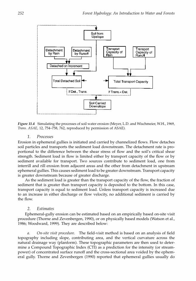
252 Forest Hydrology: An Introduction to Water and Forests
1. ProcessesErosion in ephemeral gullies is initiated and carried by channelized flows. Flow detachessoil particles and transports the sediment load downstream. The detachment rate is pro-portional to the difference between the shear stress of flow and the soil’s critical shearstrength. Sediment load in flow is limited either by transport capacity of the flow or bysediment available for transport. Two sources contribute to sediment load, one frominterrill and rill erosion from adjacent areas and the other from detachment in upstreamephemeral gullies. This causes sediment load to be greater downstream. Transport capacityis greater downstream because of greater discharge.
As the sediment load is greater than the transport capacity of the flow, the fraction ofsediment that is greater than transport capacity is deposited to the bottom. In this case,transport capacity is equal to sediment load. Unless transport capacity is increased dueto an increase in either discharge or flow velocity, no additional sediment is carried bythe flow.
2. EstimatesEphemeral-gully erosion can be estimated based on an empirically based on-site visit
procedure (Thorne and Zevenbergen, 1990), or on physically based models (Watson et al.,1986; Woodward, 1999). They are described below:
a. On-site visit procedure. The field-visit method is based on an analysis of fieldtopography including slope, contributing area, and the vertical curvature across thenatural drainage way (planform). These topographic parameters are then used to deter-mine a Compound Topographic Index (CTI) as a prediction for the intensity (or stream-power) of concentrated surface runoff and the cross-sectional area voided by the ephem-eral gully. Thorne and Zevenbergen (1990) reported that ephemeral gullies usually do
Figure 11.4 Simulating the processes of soil water erosion (Meyer, L.D. and Wischmeier, W.H., 1969,Trans. ASAE, 12, 754–758, 762, reproduced by permission of ASAE).
1363_C11_fm Page 252 Wednesday, December 4, 2002 7:44 AM
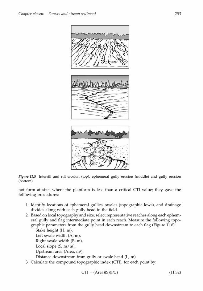
Chapter eleven: Forests and stream sediment 253
not form at sites where the planform is less than a critical CTI value; they gave thefollowing procedures:
1. Identify locations of ephemeral gullies, swales (topographic lows), and drainagedivides along with each gully head in the field.
2. Based on local topography and size, select representative reaches along each ephem-eral gully and flag intermediate point in each reach. Measure the following topo-graphic parameters from the gully head downstream to each flag (Figure 11.6):
Stake height (H, m),Left swale width (A, m),Right swale width (B, m),Local slope (S, m/m),Upstream area (Area, m2),Distance downstream from gully or swale head (L, m)
3. Calculate the compound topographic index (CTI), for each point by:
CTI = (Area)(S)(PC) (11.32)
Figure 11.5 Interrill and rill erosion (top), ephemeral gully erosion (middle) and gully erosion(bottom).
1363_C11_fm Page 253 Wednesday, December 4, 2002 7:44 AM
254 Forest Hydrology: An Introduction to Water and Forests
where PC, the planform curvature of the swale, a control on the convergence of surfacerunoff and hence the concentration of erosive streampower per unit bed area, is given by:
PC = 200(H)/[(A)(B)] (11.33)
4. Calculate the CTIcrit as the average of CTI value for all gully head points. Point CTIvalues less than the CTIcrit are excluded from further analysis because they wouldnot have an ephemeral gully in an average year.
5. Calculate the gully cross-sectional area for all points with CTI > CTIcrit by theexperimentally derived equation:
Cross-sectional area, m2 = 0.03365(CTI)0.25 (11.34)
6. Calculate the eroded volume for each reach from the cross-sectional area and thereach length. The cross-sectional area in each reach represents a distance halfwayto its upstream and downstream reaches. Summing the eroded volume in eachreach yields the annual ephemeral gully erosion for the field. Multiply the volumeby soil bulk density to yield total annual soil erosion in mass and then convert themass into mass per unit area.
b. Physical models. Physical models use two components relating hydrology andthe erosion process. The hydrology component estimates peak discharge and runoff vol-ume by use of SCS curve number, drainage area, watershed flow length, watershed slope,and 24-h rainfall and standard temporal distribution. The estimated peakflow and dis-charge volume drive the erosion component, a combination of physical-process equationsand empirical relationships to estimate the width and depth of the ephemeral gully. Finally,the mass of soil erosion is calculated using the volume voided and the soil bulk density.
A basic equation relating soil detachment from gully boundaries to flow hydraulics(Woodward, 1999) is:
De = Kch(1.35t – tc) (11.35)
where De = detachment rate (g m-2 sec-1), Kch = channel erodibility factor (g sec-1 N-1),t = average shear stress of flowing water (N m-2), tc = critical shear strength of soil (Nm–2), and the constant 1.35 is to represent maximum stress at the channel bottom. Theamount of detachment is balanced with the sediment transport capacity of the flowingwater by the equation:
De/Dc + D/Tc = 1 (11.36)
where De = detachment rate, Dc = maximum detachment capacity, D = sediment, andTc = sediment transport capacity.
The erosion process begins with a gully of initial width We. Depending on theduration of runoff, channel slope, and hydraulic roughness, the gully will continue todeepen until an erosion-resistant layer is reached. At that time further deepening ceasesand the channel begins to widen toward the ultimate width, Wu. If the flow ceases afterthe channel reaches the erosion-resistant layer but before the ultimate width is attained,it results in a width of W between We and Wu. Regression equations used to estimate
1363_C11_fm Page 254 Wednesday, December 4, 2002 7:44 AM
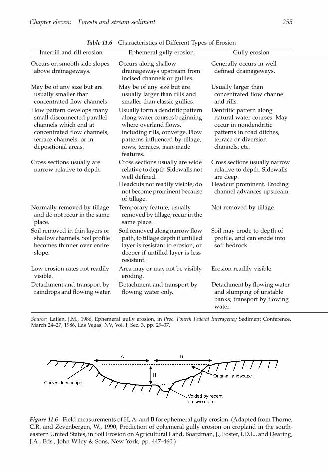
Chapter eleven: Forests and stream sediment 255
Table 11.6 Characteristics of Different Types of Erosion
Interrill and rill erosion Ephemeral gully erosion Gully erosion
Occurs on smooth side slopes above drainageways.
Occurs along shallow drainageways upstream from incised channels or gullies.
Generally occurs in well-defined drainageways.
May be of any size but are usually smaller than concentrated flow channels.
May be of any size but are usually larger than rills and smaller than classic gullies.
Usually larger than concentrated flow channel and rills.
Flow pattern develops many small disconnected parallel channels which end at concentrated flow channels, terrace channels, or in depositional areas.
Usually form a dendritic pattern along water courses beginning where overland flows, including rills, converge. Flow patterns influenced by tillage, rows, terraces, man-made features.
Dentritic pattern along natural water courses. May occur in nondendritic patterns in road ditches, terrace or diversion channels, etc.
Cross sections usually are narrow relative to depth.
Cross sections usually are wide relative to depth. Sidewalls not well defined.
Headcuts not readily visible; do not become prominent because of tillage.
Cross sections usually narrow relative to depth. Sidewalls are deep.
Headcut prominent. Eroding channel advances upstream.
Normally removed by tillage and do not recur in the same place.
Temporary feature, usually removed by tillage; recur in the same place.
Not removed by tillage.
Soil removed in thin layers or shallow channels. Soil profile becomes thinner over entire slope.
Soil removed along narrow flow path, to tillage depth if untilled layer is resistant to erosion, or deeper if untilled layer is less resistant.
Soil may erode to depth of profile, and can erode into soft bedrock.
Low erosion rates not readily visible.
Area may or may not be visibly eroding.
Erosion readily visible.
Detachment and transport by raindrops and flowing water.
Detachment and transport by flowing water only.
Detachment by flowing water and slumping of unstable banks; transport by flowing water.
Source: Laflen, J.M., 1986, Ephemeral gully erosion, in Proc. Fourth Federal Interagency Sediment Conference,March 24–27, 1986, Las Vegas, NV, Vol. I, Sec. 3, pp. 29–37.
Figure 11.6 Field measurements of H, A, and B for ephemeral gully erosion. (Adapted from Thorne,C.R. and Zevenbergen, W., 1990, Prediction of ephemeral gully erosion on cropland in the south-eastern United States, in Soil Erosion on Agricultural Land, Boardman, J., Foster, I.D.L., and Dearing,J.A., Eds., John Wiley & Sons, New York, pp. 447–460.)
1363_C11_fm Page 255 Wednesday, December 4, 2002 7:44 AM
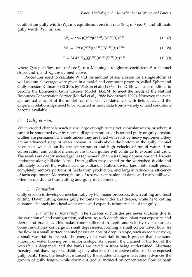
256 Forest Hydrology: An Introduction to Water and Forests
equilibrium gully width (We, m), equilibrium erosion rate (E, g m-2 sec-1), and ultimategully width (Wu, m) are:
We = 2.66 (Q0.396)(n0.387)(S–0.16)(tc)–0.24 (11.37)
Wu = 179 (Q0.552)(n0.556)(S0.199)(tc)–0.476 (11.38)
E = 34.42 Kch(Q0.811)(n0.80)(S0.77)(tc)–0.48 (11.39)
where Q = peakflow rate (m3 sec-1), n = Manning’s roughness coefficient, S = channelslope, and tc and Kch are defined above.
Procedures used to calculate W and the amount of soil erosion for a single storm aswell as annual average were given in a model and computer program, called EphemeralGully Erosion Estimator (EGEE), by Watson et al. (1986). The EGEE was later modified tobecome the Ephemeral Gully Erosion Model (EGEM) to meet the needs of the NaturalResources Conservation Service (Merkel et al., 1988; Woodward, 1999). However, the aver-age annual concept of the model has not been validated yet with field data, and theempirical relationships need to be adjusted as more data from a variety of field conditionsbecome available.
C. Gully erosion
When eroded channels reach a size large enough to restrict vehicular access or where itcannot be smoothed over by normal tillage operations, it is termed gully or gully erosion.Gullies are permanent channels unless they are filled with soils by heavy equipment; theyare an advanced stage of water erosion. All soils above the bottom in the gully channelhave been washed out by the concentration and high velocity of runoff water. If noconservation and control measures are taken, gullies will continue to expand and grow.The results are deeply incised gullies (ephemeral channels) along depressions and discretelandscape along hillside slopes. Deep gullies may extend to the watershed divide andultimately convert the watershed into badlands. Gullies divide lands into small pieces,completely remove portions of fields from production, and largely reduce the efficiencyof farm equipment. Moreover, failure of reservoir-embankment dams and earth spillwaysoften occurs due to head cutting and gully development.
1. FormationGully erosion is developed mechanically by two major processes, down cutting and headcutting. Down cutting causes gully bottoms to be wider and deeper, while head cuttingadvances channels into headwater areas and expands tributary nets of the gully.
a. Induced by surface runoff. The surfaces of hillsides are never uniform due tothe variation of land configuration, soil texture, rock distribution, plant root exposure, anddebris and branches. This makes runoff different in depth and velocity over a surface.Some runoff may converge in small depressions, forming a small concentrated flow. Asthe flow in a small surface channel passes an abrupt drop in slope, such as roots or rocks,a small waterfall is created. The energy of a waterfall is much greater than the sameamount of water flowing on a uniform slope. As a result, the channel at the foot of thewaterfall is deepened, and the banks are caved in from being undermined. Alternatefreezing and thawing or landsliding may also result in massive collapse of the exposedgully bank. Thus, the head-cut induced by the sudden change in elevation advances thegrowth of gully length, while down-cut (scour) induced by concentrated flow or bank
1363_C11_fm Page 256 Wednesday, December 4, 2002 7:44 AM
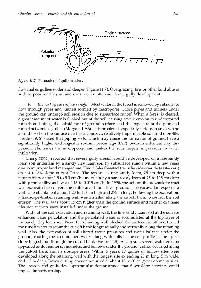
Chapter eleven: Forests and stream sediment 257
flow makes gullies wider and deeper (Figure 11.7). Overgrazing, fire, or other land abusessuch as poor road layout and construction often accelerate gully development.
b. Induced by subsurface runoff. Most water in the forest is removed by subsurfaceflow through pipes and tunnels formed by macropores. Those pipes and tunnels underthe ground can undergo soil erosion due to subsurface runoff. When a forest is cleared,a great amount of water is flushed out of the soil, causing severe erosion to undergroundtunnels and pipes, the subsidence of ground surface, and the exposure of the pipe andtunnel network as gullies (Morgan, 1986). This problem is especially serious in areas wherea sandy soil on the surface overlies a compact, relatively impermeable soil in the profile.Heede (1976) stated that piping soils, which may cause the formation of gullies, have asignificantly higher exchangeable sodium percentage (ESP). Sodium enhances clay dis-persion, eliminates the macropores, and makes the soils largely impervious to waterinfiltration.
Chang (1997) reported that severe gully erosion could be developed on a fine sandyloam soil underlain by a sandy clay loam soil by subsurface runoff within a few yearsdue to improper land management. Two 2.8-ha forested tracts lie side-by-side (east–west)on a 4 to 8% slope in east Texas. The top soil is fine sandy loam, 75 cm deep with apermeability about 1.5 to 5.0 cm/h, underlain by a sandy clay loam at 75 to 125 cm deepwith permeability as low as 0.15 to 0.015 cm/h. In 1990, the soil on the downslope tractwas excavated to convert the entire area into a level ground. The excavation exposed avertical embankment about 1.20 to 1.50 m high and 275 m long. Following the excavation,a landscape-timber retaining wall was installed along the cut-off bank to control the soilerosion. The wall was about 15 cm higher than the ground surface and neither drainagetiles nor anchors were installed under the ground.
Without the soil excavation and retaining wall, the fine sandy loam soil at the surfaceenhances water percolation and the percolated water is accumulated at the top layer ofthe sandy clay loam soil. Now, the retaining wall blocked the surface runoff and turnedthe runoff water to scour the cut-off bank longitudinally and vertically along the retainingwall. Also, the excavation of soil altered water pressures and water balance under theground, causing the accumulated water along with soils in the soil profile in the upperslope to gush out through the cut-off bank (Figure 11.8). As a result, severe water erosionappeared as depressions, sinkholes, and hollows under the ground; gullies occurred alongthe cut-off bank and its upslope areas. Within 5 years, 17 gullies or hollow sites weredeveloped along the retaining wall with the longest site extending 25 m long, 5 m wide,and 1.5 m deep. Down-cutting erosion occurred at about 15 to 30 cm/year on many sites.The erosion and gully development also demonstrated that downslope activities couldimpose impacts upslope.
Figure 11.7 Formation of gully erosion.
1363_C11_fm Page 257 Wednesday, December 4, 2002 7:44 AM
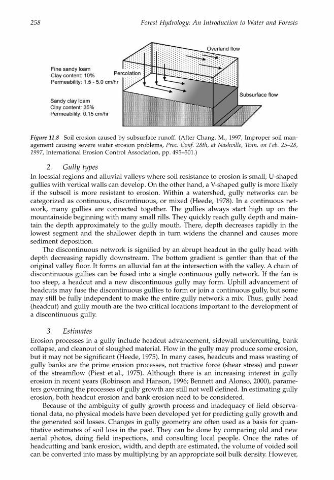
258 Forest Hydrology: An Introduction to Water and Forests
2. Gully typesIn loessial regions and alluvial valleys where soil resistance to erosion is small, U-shapedgullies with vertical walls can develop. On the other hand, a V-shaped gully is more likelyif the subsoil is more resistant to erosion. Within a watershed, gully networks can becategorized as continuous, discontinuous, or mixed (Heede, 1978). In a continuous net-work, many gullies are connected together. The gullies always start high up on themountainside beginning with many small rills. They quickly reach gully depth and main-tain the depth approximately to the gully mouth. There, depth decreases rapidly in thelowest segment and the shallower depth in turn widens the channel and causes moresediment deposition.
The discontinuous network is signified by an abrupt headcut in the gully head withdepth decreasing rapidly downstream. The bottom gradient is gentler than that of theoriginal valley floor. It forms an alluvial fan at the intersection with the valley. A chain ofdiscontinuous gullies can be fused into a single continuous gully network. If the fan istoo steep, a headcut and a new discontinuous gully may form. Uphill advancement ofheadcuts may fuse the discontinuous gullies to form or join a continuous gully, but somemay still be fully independent to make the entire gully network a mix. Thus, gully head(headcut) and gully mouth are the two critical locations important to the development ofa discontinuous gully.
3. EstimatesErosion processes in a gully include headcut advancement, sidewall undercutting, bankcollapse, and cleanout of sloughed material. Flow in the gully may produce some erosion,but it may not be significant (Heede, 1975). In many cases, headcuts and mass wasting ofgully banks are the prime erosion processes, not tractive force (shear stress) and powerof the streamflow (Piest et al., 1975). Although there is an increasing interest in gullyerosion in recent years (Robinson and Hanson, 1996; Bennett and Alonso, 2000), parame-ters governing the processes of gully growth are still not well defined. In estimating gullyerosion, both headcut erosion and bank erosion need to be considered.
Because of the ambiguity of gully growth process and inadequacy of field observa-tional data, no physical models have been developed yet for predicting gully growth andthe generated soil losses. Changes in gully geometry are often used as a basis for quan-titative estimates of soil loss in the past. They can be done by comparing old and newaerial photos, doing field inspections, and consulting local people. Once the rates ofheadcutting and bank erosion, width, and depth are estimated, the volume of voided soilcan be converted into mass by multiplying by an appropriate soil bulk density. However,
Figure 11.8 Soil erosion caused by subsurface runoff. (After Chang, M., 1997, Improper soil man-agement causing severe water erosion problems, Proc. Conf. 28th, at Nashville, Tenn. on Feb. 25–28,1997, International Erosion Control Association, pp. 495–501.)
1363_C11_fm Page 258 Wednesday, December 4, 2002 7:44 AM
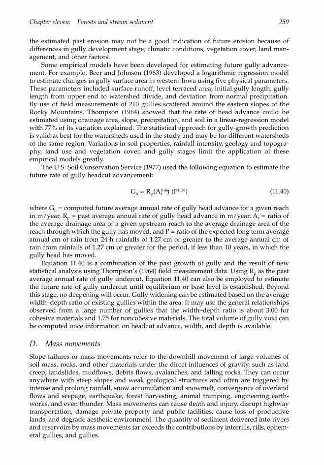
Chapter eleven: Forests and stream sediment 259
the estimated past erosion may not be a good indication of future erosion because ofdifferences in gully development stage, climatic conditions, vegetation cover, land man-agement, and other factors.
Some empirical models have been developed for estimating future gully advance-ment. For example, Beer and Johnson (1963) developed a logarithmic regression modelto estimate changes in gully surface area in western Iowa using five physical parameters.These parameters included surface runoff, level terraced area, initial gully length, gullylength from upper end to watershed divide, and deviation from normal precipitation.By use of field measurements of 210 gullies scattered around the eastern slopes of theRocky Mountains, Thompson (1964) showed that the rate of head advance could beestimated using drainage area, slope, precipitation, and soil in a linear-regression modelwith 77% of its variation explained. The statistical approach for gully-growth predictionis valid at best for the watersheds used in the study and may be for different watershedsof the same region. Variations in soil properties, rainfall intensity, geology and topogra-phy, land use and vegetation cover, and gully stages limit the application of theseempirical models greatly.
The U.S. Soil Conservation Service (1977) used the following equation to estimate thefuture rate of gully headcut advancement:
Gh = Rp(Ar0.46) (P0.20) (11.40)
where Gh = computed future average annual rate of gully head advance for a given reachin m/year, Rp = past average annual rate of gully head advance in m/year, Ar = ratio ofthe average drainage area of a given upstream reach to the average drainage area of thereach through which the gully has moved, and P = ratio of the expected long term averageannual cm of rain from 24-h rainfalls of 1.27 cm or greater to the average annual cm ofrain from rainfalls of 1.27 cm or greater for the period, if less than 10 years, in which thegully head has moved.
Equation 11.40 is a combination of the past growth of gully and the result of newstatistical analysis using Thompson’s (1964) field measurement data. Using Rp as the pastaverage annual rate of gully undercut, Equation 11.40 can also be employed to estimatethe future rate of gully undercut until equilibrium or base level is established. Beyondthis stage, no deepening will occur. Gully widening can be estimated based on the averagewidth–depth ratio of existing gullies within the area. It may use the general relationshipsobserved from a large number of gullies that the width–depth ratio is about 3.00 forcohesive materials and 1.75 for noncohesive materials. The total volume of gully void canbe computed once information on headcut advance, width, and depth is available.
D. Mass movements
Slope failures or mass movements refer to the downhill movement of large volumes ofsoil mass, rocks, and other materials under the direct influences of gravity, such as landcreep, landslides, mudflows, debris flows, avalanches, and falling rocks. They can occuranywhere with steep slopes and weak geological structures and often are triggered byintense and prolong rainfall, snow accumulation and snowmelt, convergence of overlandflows and seepage, earthquake, forest harvesting, animal tramping, engineering earth-works, and even thunder. Mass movements can cause death and injury, disrupt highwaytransportation, damage private property and public facilities, cause loss of productivelands, and degrade aesthetic environment. The quantity of sediment delivered into riversand reservoirs by mass movements far exceeds the contributions by interrills, rills, ephem-eral gullies, and gullies.
1363_C11_fm Page 259 Wednesday, December 4, 2002 7:44 AM
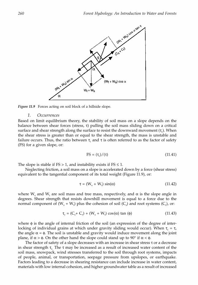
260 Forest Hydrology: An Introduction to Water and Forests
1. OccurrencesBased on limit equilibrium theory, the stability of soil mass on a slope depends on thebalance between shear forces (stress, t) pulling the soil mass sliding down on a criticalsurface and shear strength along the surface to resist the downward movement (tc). Whenthe shear stress is greater than or equal to the shear strength, the mass is unstable andfailure occurs. Thus, the ratio between tc and t is often referred to as the factor of safety(FS) for a given slope, or:
FS = (tc)/(t) (11.41)
The slope is stable if FS > 1, and instability exists if FS £ 1.Neglecting friction, a soil mass on a slope is accelerated down by a force (shear stress)
equivalent to the tangential component of its total weight (Figure 11.9), or:
t = (Ws + Wt) sin(a) (11.42)
where Ws and Wt are soil mass and tree mass, respectively, and a is the slope angle indegrees. Shear strength that resists downhill movement is equal to a force due to thenormal component of (Ws + Wt) plus the cohesion of soil (Cs) and root systems (Cr), or:
tc = (Cs+ Cr) + (Ws + Wt) cos(a) tan (f) (11.43)
where f is the angle of internal friction of the soil (an expression of the degree of inter-locking of individual grains at which under gravity sliding would occur). When tc = t,the angle a = f. The soil is unstable and gravity would induce movement along the jointplane, if a > f. On the other hand the slope could stand up to 90∞ if a < f.
The factor of safety of a slope decreases with an increase in shear stress t or a decreasein shear strength tc. The t may be increased as a result of increased water content of thesoil mass, snowpack, wind stresses transferred to the soil through root systems, impactsof people, animal, or transportation, seepage pressure from upslopes, or earthquake.Factors leading to a decrease in shearing resistance can include increase in water content,materials with low internal cohesion, and higher groundwater table as a result of increased
Figure 11.9 Forces acting on soil block of a hillside slope.
1363_C11_fm Page 260 Wednesday, December 4, 2002 7:44 AM
Chapter eleven: Forests and stream sediment 261
precipitation, deforestation, and dam construction. In any case, slope instability is seldoma single-cause event; it usually results from a series of events that lead to mass movements.
Forest vegetation tends to maintain more-secure slopes by mechanisms transferredthrough its canopy and root systems. They include:
1. Mechanical reinforcement of root systems that transfers shear stress in the soil totensile resistance in the roots
2. Depletion of soil moisture by interception, transpiration, snow accumulation, andsnowmelt that limit the buildup of positive water pressure
3. Increasing soil organic matter content that strengthens the cohesion of soil4. Buttressing or soil arching action between trunks and stems that counteracts downs-
lope shear forces
Thus, forest harvesting and related activities on steep terrain often cause slope insta-bility and mass movements. Perhaps the most significant effect of vegetation removal ison root reinforcement. Studies showed that landslides were most frequent 4 to 10 yearsafter logging (Gray and Megahan, 1981). The time of occurrence of maximum landslidehazard seems to be affected by the relative rates of root decay and new root growth.
In southwestern Oregon, the rates of mass erosion from debris slides in disturbedareas were on average five times greater than in undisturbed forest sites. Mass erosionwas more than 100 times greater in disturbed road rights-of-way areas than on undisturbednatural slopes (Amaranthus et al., 1985). Road construction was also the most likely causeof accelerated landslide activity in the Idaho Batholith area. Combining road constructionwith logging and forest fires accounted for 88% of total landslides, and the removal ofvegetation accounted for 9%. Only 3% of the landslides occurred on slopes with nodisturbance (Megahan et al., 1978).
2. EstimatesBecause of its size and site specificity, mass erosion is usually estimated based on volu-metric measurements made in the field or through aerial-photo interpretations. Moderntechnologies such as geographic information systems (GIS) and geographic position sys-tems (GPS) can also be employed for large-scale digital mapping and data analysis.Combining these technologies with field reconnaissance and calibration provides morereliable estimates. Once the voided volume of mass movements is available, multiplyingthe volume by soil density yields the total mass of landslides.
E. Channel erosion
Channel erosion applies to channels in the lower end of headwater tributaries with waterflowing all year around, while gully erosion refers to those channels in the upper ends ofheadwater tributaries with water flowing during or immediately after storms. Channelerosion consists of soil erosion on stream bank and sediment transport in the streamchannel.
1. Stream-bank erosionErosion on stream bank is caused by raindrop splash, surface runoff, the scouring andundercutting of water by the processes of corrosion (chemical reaction of water and rocks),corrasion (grinding action of sediment), cavitation (kinetic and potential of the stream,wave actions), and gravitation. Frequently, stream-bank erosion is accelerated by theremoval of vegetation, grazing, tillage near the bank, and stream crossing by vehicles andanimals. However, the continuous movement (kinetic energy) of water is mainly respon-
1363_C11_fm Page 261 Wednesday, December 4, 2002 7:44 AM
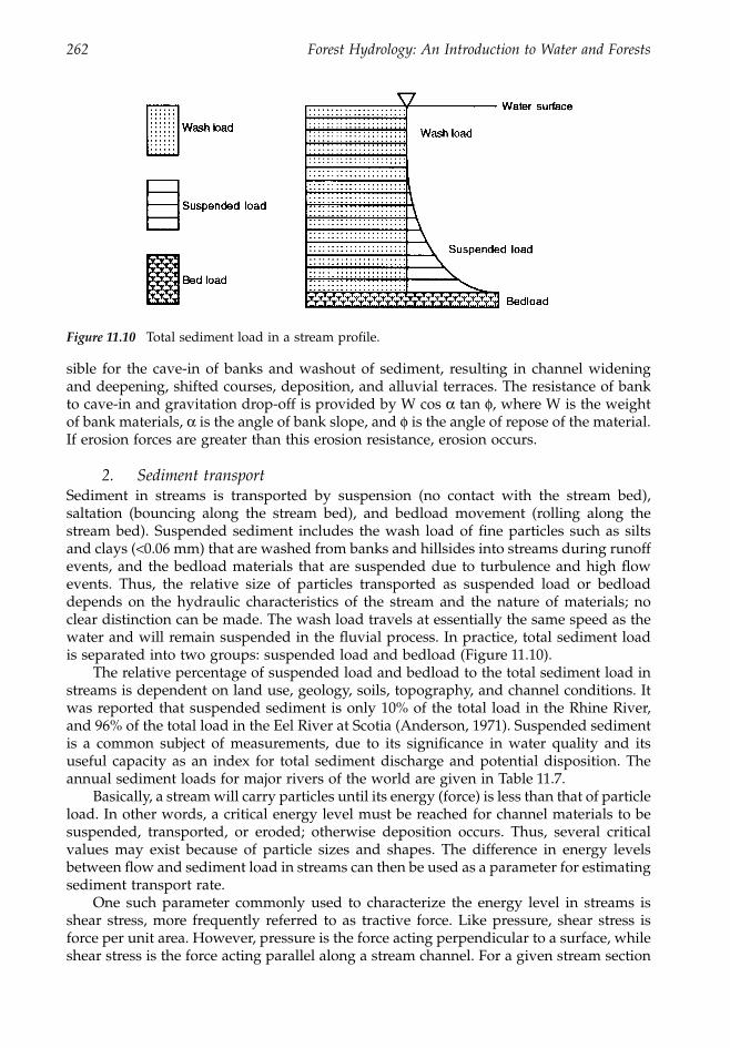
262 Forest Hydrology: An Introduction to Water and Forests
sible for the cave-in of banks and washout of sediment, resulting in channel wideningand deepening, shifted courses, deposition, and alluvial terraces. The resistance of bankto cave-in and gravitation drop-off is provided by W cos a tan f, where W is the weightof bank materials, a is the angle of bank slope, and f is the angle of repose of the material.If erosion forces are greater than this erosion resistance, erosion occurs.
2. Sediment transportSediment in streams is transported by suspension (no contact with the stream bed),saltation (bouncing along the stream bed), and bedload movement (rolling along thestream bed). Suspended sediment includes the wash load of fine particles such as siltsand clays (<0.06 mm) that are washed from banks and hillsides into streams during runoffevents, and the bedload materials that are suspended due to turbulence and high flowevents. Thus, the relative size of particles transported as suspended load or bedloaddepends on the hydraulic characteristics of the stream and the nature of materials; noclear distinction can be made. The wash load travels at essentially the same speed as thewater and will remain suspended in the fluvial process. In practice, total sediment loadis separated into two groups: suspended load and bedload (Figure 11.10).
The relative percentage of suspended load and bedload to the total sediment load instreams is dependent on land use, geology, soils, topography, and channel conditions. Itwas reported that suspended sediment is only 10% of the total load in the Rhine River,and 96% of the total load in the Eel River at Scotia (Anderson, 1971). Suspended sedimentis a common subject of measurements, due to its significance in water quality and itsuseful capacity as an index for total sediment discharge and potential disposition. Theannual sediment loads for major rivers of the world are given in Table 11.7.
Basically, a stream will carry particles until its energy (force) is less than that of particleload. In other words, a critical energy level must be reached for channel materials to besuspended, transported, or eroded; otherwise deposition occurs. Thus, several criticalvalues may exist because of particle sizes and shapes. The difference in energy levelsbetween flow and sediment load in streams can then be used as a parameter for estimatingsediment transport rate.
One such parameter commonly used to characterize the energy level in streams isshear stress, more frequently referred to as tractive force. Like pressure, shear stress isforce per unit area. However, pressure is the force acting perpendicular to a surface, whileshear stress is the force acting parallel along a stream channel. For a given stream section
Figure 11.10 Total sediment load in a stream profile.
1363_C11_fm Page 262 Wednesday, December 4, 2002 7:44 AM
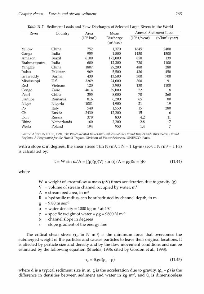
Chapter eleven: Forests and stream sediment 263
with a slope a in degrees, the shear stress t (in N/m2, 1 N = 1 kg-m/sec2; 1 N/m2 = 1 Pa)is calculated by:
t = W sin a/A = [(r)(g)(V) sin a]/A = rgRs = gRs (11.44)
where
W = weight of streamflow = mass (rV) times acceleration due to gravity (g)V = volume of stream channel occupied by water, m3
A = stream bed area, in m2
R = hydraulic radius, can be substituted by channel depth, in mg = 9.80 m sec-2
r = water density = 1000 kg m-3 at 4∞Cg = specific weight of water = rg = 9800 N m-3
a = channel slope in degreess = slope gradient of the energy line
The critical shear stress (tc, in N m-2) is the minimum force that overcomes thesubmerged weight of the particles and causes particles to leave their original locations. Itis affected by particle size and density and by the flow movement conditions and can beestimated by the following equation (Shields, 1936; cited by Gordon et al., 1993):
tc = qcgd(rs – r) (11.45)
where d is a typical sediment size in m, g is the acceleration due to gravity, (rs - r) is thedifference in densities between sediment and water in kg m-3, and qc is dimensionless
Table 11.7 Sediment Loads and Flow Discharges of Selected Large Rivers in the World
River Country Area(103 km3)
Mean Discharge(m3/sec)
Annual Sediment Load(103 t/year) (t/km2/year)
Yellow China 752 1,370 1645 2480Ganga India 955 1,800 1450 1500Amazon Brazil 6100 172,000 850 139Brahmapputra India 600 12,200 730 1100Yangtze China 1807 29,200 480 280Indus Pakistan 969 5,500 436 450Irrawaddy Burma 430 13,500 300 700Mississippi U.S. 3269 24,000 300 91Red Vietnam 120 3,900 130 1100Congo Zaire 4014 39,000 72 18Pearl China 355 8,000 70 260Danube Romania 816 6,200 65 80Niger Nigeria 1081 4,900 21 19Po Italy 540 1,550 15 280Ob Russia 2430 12,200 15 6Don Russia 378 830 4.2 11Rhine Netherlands 160 2,200 2.8 17Wesla Poland 194 950 1.4 7
Source: After UNESCO, 1991, The Water-Related Issues and Problems of the Humid Tropics and Other Warm HumidRegions: A Programme for the Humid Tropics, Division of Water Sciences, UNESCO. Paris.
1363_C11_fm Page 263 Wednesday, December 4, 2002 7:44 AM
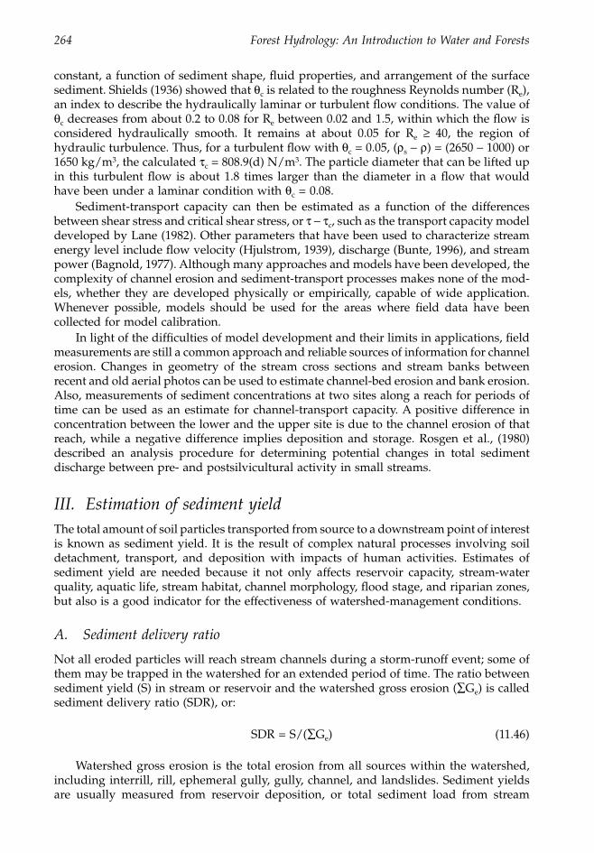
264 Forest Hydrology: An Introduction to Water and Forests
constant, a function of sediment shape, fluid properties, and arrangement of the surfacesediment. Shields (1936) showed that qc is related to the roughness Reynolds number (Re),an index to describe the hydraulically laminar or turbulent flow conditions. The value ofqc decreases from about 0.2 to 0.08 for Re between 0.02 and 1.5, within which the flow isconsidered hydraulically smooth. It remains at about 0.05 for Re ≥ 40, the region ofhydraulic turbulence. Thus, for a turbulent flow with qc = 0.05, (rs - r) = (2650 - 1000) or1650 kg/m3, the calculated tc = 808.9(d) N/m3. The particle diameter that can be lifted upin this turbulent flow is about 1.8 times larger than the diameter in a flow that wouldhave been under a laminar condition with qc = 0.08.
Sediment-transport capacity can then be estimated as a function of the differencesbetween shear stress and critical shear stress, or t - tc, such as the transport capacity modeldeveloped by Lane (1982). Other parameters that have been used to characterize streamenergy level include flow velocity (Hjulstrom, 1939), discharge (Bunte, 1996), and streampower (Bagnold, 1977). Although many approaches and models have been developed, thecomplexity of channel erosion and sediment-transport processes makes none of the mod-els, whether they are developed physically or empirically, capable of wide application.Whenever possible, models should be used for the areas where field data have beencollected for model calibration.
In light of the difficulties of model development and their limits in applications, fieldmeasurements are still a common approach and reliable sources of information for channelerosion. Changes in geometry of the stream cross sections and stream banks betweenrecent and old aerial photos can be used to estimate channel-bed erosion and bank erosion.Also, measurements of sediment concentrations at two sites along a reach for periods oftime can be used as an estimate for channel-transport capacity. A positive difference inconcentration between the lower and the upper site is due to the channel erosion of thatreach, while a negative difference implies deposition and storage. Rosgen et al., (1980)described an analysis procedure for determining potential changes in total sedimentdischarge between pre- and postsilvicultural activity in small streams.
III. Estimation of sediment yieldThe total amount of soil particles transported from source to a downstream point of interestis known as sediment yield. It is the result of complex natural processes involving soildetachment, transport, and deposition with impacts of human activities. Estimates ofsediment yield are needed because it not only affects reservoir capacity, stream-waterquality, aquatic life, stream habitat, channel morphology, flood stage, and riparian zones,but also is a good indicator for the effectiveness of watershed-management conditions.
A. Sediment delivery ratio
Not all eroded particles will reach stream channels during a storm-runoff event; some ofthem may be trapped in the watershed for an extended period of time. The ratio betweensediment yield (S) in stream or reservoir and the watershed gross erosion (ÂGe) is calledsediment delivery ratio (SDR), or:
SDR = S/(ÂGe) (11.46)
Watershed gross erosion is the total erosion from all sources within the watershed,including interrill, rill, ephemeral gully, gully, channel, and landslides. Sediment yieldsare usually measured from reservoir deposition, or total sediment load from stream
1363_C11_fm Page 264 Wednesday, December 4, 2002 7:44 AM
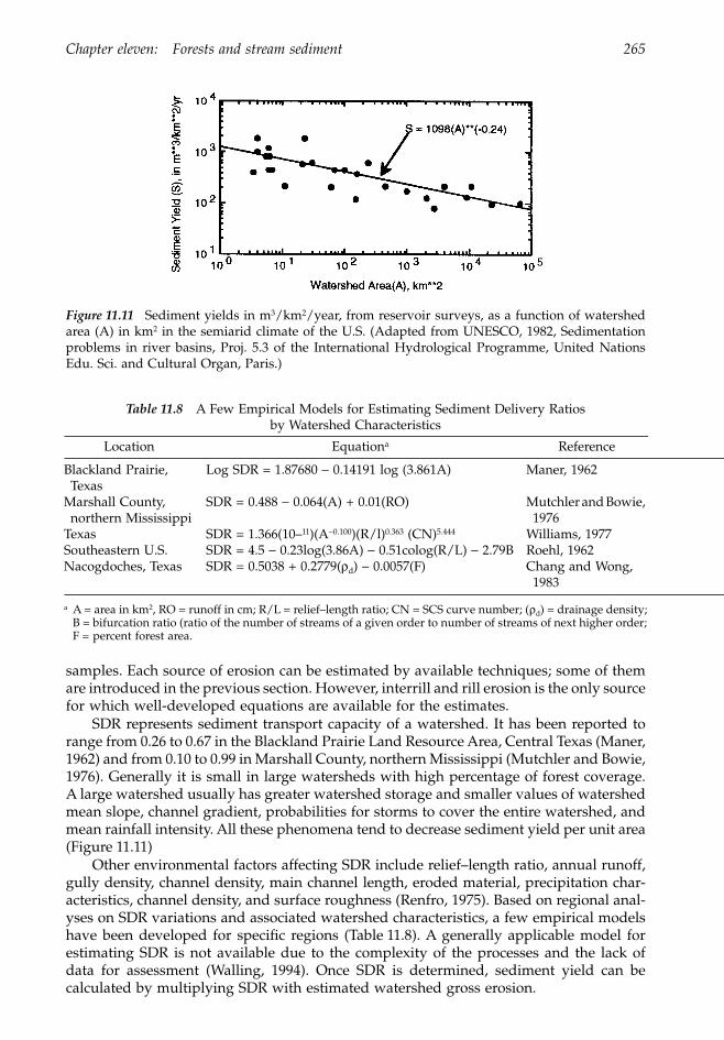
Chapter eleven: Forests and stream sediment 265
samples. Each source of erosion can be estimated by available techniques; some of themare introduced in the previous section. However, interrill and rill erosion is the only sourcefor which well-developed equations are available for the estimates.
SDR represents sediment transport capacity of a watershed. It has been reported torange from 0.26 to 0.67 in the Blackland Prairie Land Resource Area, Central Texas (Maner,1962) and from 0.10 to 0.99 in Marshall County, northern Mississippi (Mutchler and Bowie,1976). Generally it is small in large watersheds with high percentage of forest coverage.A large watershed usually has greater watershed storage and smaller values of watershedmean slope, channel gradient, probabilities for storms to cover the entire watershed, andmean rainfall intensity. All these phenomena tend to decrease sediment yield per unit area(Figure 11.11)
Other environmental factors affecting SDR include relief–length ratio, annual runoff,gully density, channel density, main channel length, eroded material, precipitation char-acteristics, channel density, and surface roughness (Renfro, 1975). Based on regional anal-yses on SDR variations and associated watershed characteristics, a few empirical modelshave been developed for specific regions (Table 11.8). A generally applicable model forestimating SDR is not available due to the complexity of the processes and the lack ofdata for assessment (Walling, 1994). Once SDR is determined, sediment yield can becalculated by multiplying SDR with estimated watershed gross erosion.
Figure 11.11 Sediment yields in m3/km2/year, from reservoir surveys, as a function of watershedarea (A) in km2 in the semiarid climate of the U.S. (Adapted from UNESCO, 1982, Sedimentationproblems in river basins, Proj. 5.3 of the International Hydrological Programme, United NationsEdu. Sci. and Cultural Organ, Paris.)
Table 11.8 A Few Empirical Models for Estimating Sediment Delivery Ratios by Watershed Characteristics
Location Equationa Reference
Blackland Prairie, Texas
Log SDR = 1.87680 - 0.14191 log (3.861A) Maner, 1962
Marshall County, northern Mississippi
SDR = 0.488 - 0.064(A) + 0.01(RO) Mutchler and Bowie, 1976
Texas SDR = 1.366(10–11)(A-0.100)(R/l)0.363 (CN)5.444 Williams, 1977Southeastern U.S. SDR = 4.5 - 0.23log(3.86A) - 0.51colog(R/L) - 2.79B Roehl, 1962Nacogdoches, Texas SDR = 0.5038 + 0.2779(rd) - 0.0057(F) Chang and Wong,
1983
a A = area in km2, RO = runoff in cm; R/L = relief–length ratio; CN = SCS curve number; (rd) = drainage density;B = bifurcation ratio (ratio of the number of streams of a given order to number of streams of next higher order;F = percent forest area.
1363_C11_fm Page 265 Wednesday, December 4, 2002 7:44 AM
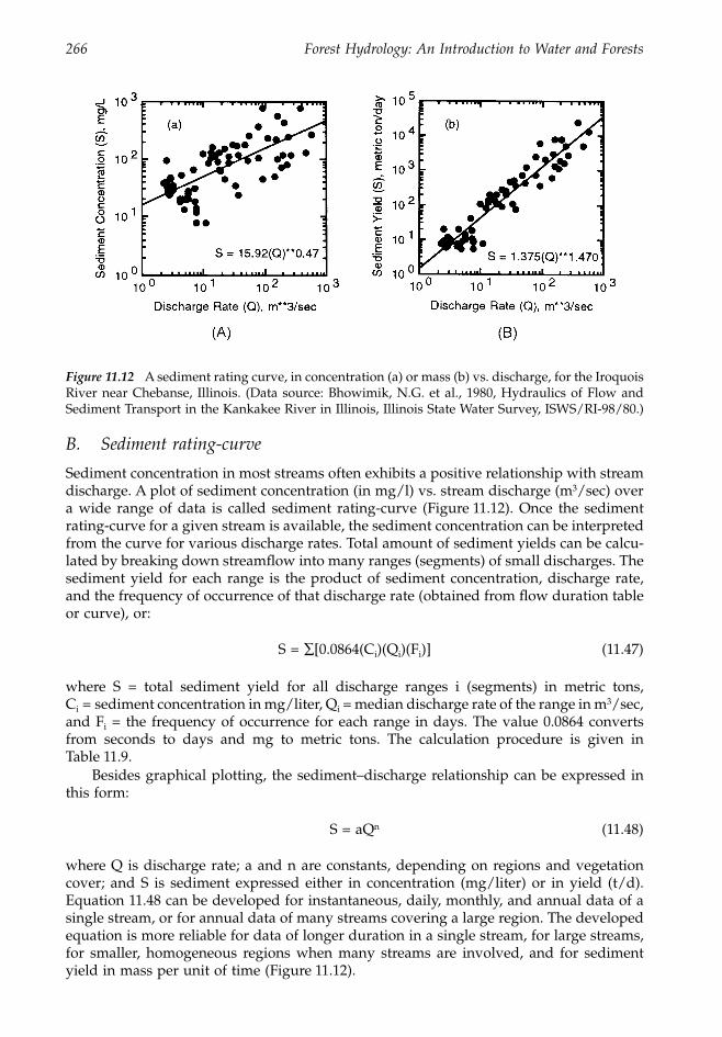
266 Forest Hydrology: An Introduction to Water and Forests
B. Sediment rating-curve
Sediment concentration in most streams often exhibits a positive relationship with streamdischarge. A plot of sediment concentration (in mg/l) vs. stream discharge (m3/sec) overa wide range of data is called sediment rating-curve (Figure 11.12). Once the sedimentrating-curve for a given stream is available, the sediment concentration can be interpretedfrom the curve for various discharge rates. Total amount of sediment yields can be calcu-lated by breaking down streamflow into many ranges (segments) of small discharges. Thesediment yield for each range is the product of sediment concentration, discharge rate,and the frequency of occurrence of that discharge rate (obtained from flow duration tableor curve), or:
S = Â[0.0864(Ci)(Qi)(Fi)] (11.47)
where S = total sediment yield for all discharge ranges i (segments) in metric tons,Ci = sediment concentration in mg/liter, Qi = median discharge rate of the range in m3/sec,and Fi = the frequency of occurrence for each range in days. The value 0.0864 convertsfrom seconds to days and mg to metric tons. The calculation procedure is given inTable 11.9.
Besides graphical plotting, the sediment–discharge relationship can be expressed inthis form:
S = aQn (11.48)
where Q is discharge rate; a and n are constants, depending on regions and vegetationcover; and S is sediment expressed either in concentration (mg/liter) or in yield (t/d).Equation 11.48 can be developed for instantaneous, daily, monthly, and annual data of asingle stream, or for annual data of many streams covering a large region. The developedequation is more reliable for data of longer duration in a single stream, for large streams,for smaller, homogeneous regions when many streams are involved, and for sedimentyield in mass per unit of time (Figure 11.12).
Figure 11.12 A sediment rating curve, in concentration (a) or mass (b) vs. discharge, for the IroquoisRiver near Chebanse, Illinois. (Data source: Bhowimik, N.G. et al., 1980, Hydraulics of Flow andSediment Transport in the Kankakee River in Illinois, Illinois State Water Survey, ISWS/RI-98/80.)
1363_C11_fm Page 266 Wednesday, December 4, 2002 7:44 AM
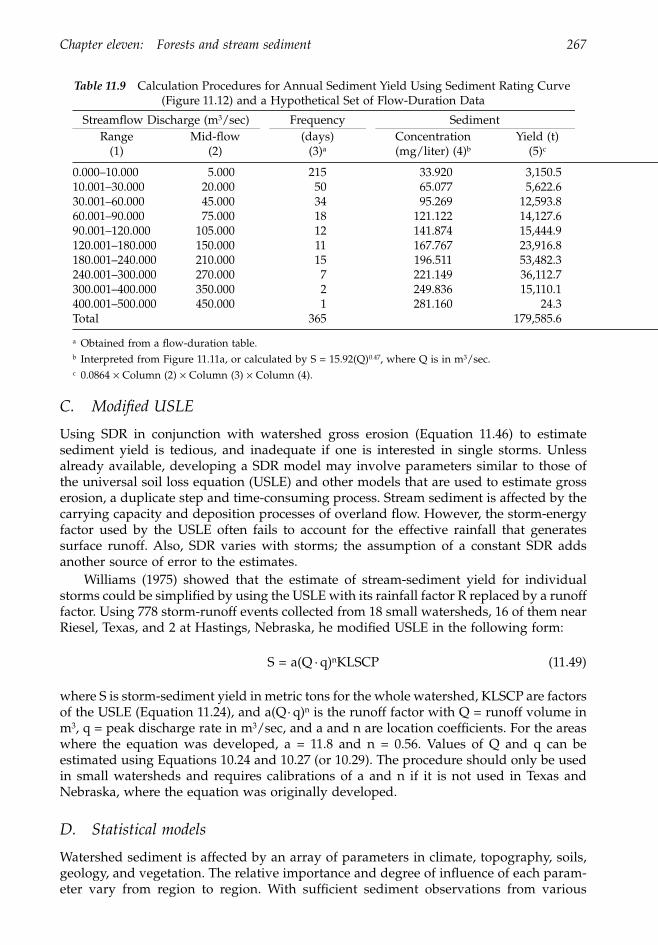
Chapter eleven: Forests and stream sediment 267
C. Modified USLE
Using SDR in conjunction with watershed gross erosion (Equation 11.46) to estimatesediment yield is tedious, and inadequate if one is interested in single storms. Unlessalready available, developing a SDR model may involve parameters similar to those ofthe universal soil loss equation (USLE) and other models that are used to estimate grosserosion, a duplicate step and time-consuming process. Stream sediment is affected by thecarrying capacity and deposition processes of overland flow. However, the storm-energyfactor used by the USLE often fails to account for the effective rainfall that generatessurface runoff. Also, SDR varies with storms; the assumption of a constant SDR addsanother source of error to the estimates.
Williams (1975) showed that the estimate of stream-sediment yield for individualstorms could be simplified by using the USLE with its rainfall factor R replaced by a runofffactor. Using 778 storm-runoff events collected from 18 small watersheds, 16 of them nearRiesel, Texas, and 2 at Hastings, Nebraska, he modified USLE in the following form:
S = a(Q · q)nKLSCP (11.49)
where S is storm-sediment yield in metric tons for the whole watershed, KLSCP are factorsof the USLE (Equation 11.24), and a(Q· q)n is the runoff factor with Q = runoff volume inm3, q = peak discharge rate in m3/sec, and a and n are location coefficients. For the areaswhere the equation was developed, a = 11.8 and n = 0.56. Values of Q and q can beestimated using Equations 10.24 and 10.27 (or 10.29). The procedure should only be usedin small watersheds and requires calibrations of a and n if it is not used in Texas andNebraska, where the equation was originally developed.
D. Statistical models
Watershed sediment is affected by an array of parameters in climate, topography, soils,geology, and vegetation. The relative importance and degree of influence of each param-eter vary from region to region. With sufficient sediment observations from various
Table 11.9 Calculation Procedures for Annual Sediment Yield Using Sediment Rating Curve (Figure 11.12) and a Hypothetical Set of Flow-Duration Data
Streamflow Discharge (m3/sec) Frequency (days)
(3)a
SedimentRange
(1)Mid-flow
(2)Concentration (mg/liter) (4)b
Yield (t)(5)c
0.000–10.000 5.000 215 33.920 3,150.510.001–30.000 20.000 50 65.077 5,622.630.001–60.000 45.000 34 95.269 12,593.860.001–90.000 75.000 18 121.122 14,127.690.001–120.000 105.000 12 141.874 15,444.9120.001–180.000 150.000 11 167.767 23,916.8180.001–240.000 210.000 15 196.511 53,482.3240.001–300.000 270.000 7 221.149 36,112.7300.001–400.000 350.000 2 249.836 15,110.1400.001–500.000 450.000 1 281.160 24.3Total 365 179,585.6
a Obtained from a flow-duration table.b Interpreted from Figure 11.11a, or calculated by S = 15.92(Q)0.47, where Q is in m3/sec.c 0.0864 ¥ Column (2) ¥ Column (3) ¥ Column (4).
1363_C11_fm Page 267 Wednesday, December 4, 2002 7:44 AM
268 Forest Hydrology: An Introduction to Water and Forests
watersheds, a statistical model can be developed relating sediment yield to environmentalparameters. Numerous models have been developed around the world (Flaxman, 1972;Walling, 1974; Renard, 1980). Parameters used in the predictions include one or a few ofthe following: watershed area, slope, channel gradient, precipitation, temperature, meandischarge and various return periods, percentage of lakes and forested areas, drainagedensity, basin form factors, and others. However, these models generally can be appliedin the regions where data were collected.
Dendy and Bolton (1976) used sediment data collected from 800 reservoirs withwatershed areas of 2.59 km2 or larger and developed the following equations to estimatesediment yield S in metric ton/km2/year (converted from English units) in the U.S.:
For Q < 5.0 cm:
S = 292Q0.46(1.54 – 0.26 log A) (11.50)
For Q ≥ 5.0 cm:
S = 686e–0.022Q(1.54 – 0.26 log A) (11.51)
where A is watershed area (in km2) and Q is annual runoff (in cm). Parameters Q and Aexplained 75% of the variation of sediment yields. However, these two equations weredeveloped from average values of grouped data, which provide an approximation forpreliminary watershed planning on a regional basis. Application of these equations toindividual watersheds, due to local factors, may produce errors as much as 10 to 100 timeslarger or smaller than actual sediment yields.
E. Physical models
The limitations of statistical models can be overcome if models are developed based onerosion processes and transport mechanisms. Many of these models use the concept thatrainfall and runoff energy must be greater than soil resistance in order to detach soilparticles. If sediment detachment (supply) is greater than flow-transport capacity, thensediment yield is equal to sediment capacity. On the other hand, if sediment supply isless than the flow transport capacity, then sediment yield is equal to sediment supply plusdetached particles. Thus, two components of models must be developed. One is thehydrology component to predict sequential flow volume and rates from storm precipita-tion and soil characteristics, and the other is the erosion component to predict soil detach-ment, transport, and sediment yield using data simulated in the hydrology component.It is important that the developed models be calibrated with field data before applicationto various management and decision-making processes.
IV. Vegetation effectsVegetation is considered a highly effective, economical, relatively permanent, and almostmaintenance-free approach to controlling soil erosion and stream sediment. Vegetationmechanisms that enhance these beneficial effects, plant characteristics that need to beexamined for specific conservation purposes, and field observations that provide lessonsand evidences of vegetation effects are briefly discussed here.
1363_C11_fm Page 268 Wednesday, December 4, 2002 7:44 AM
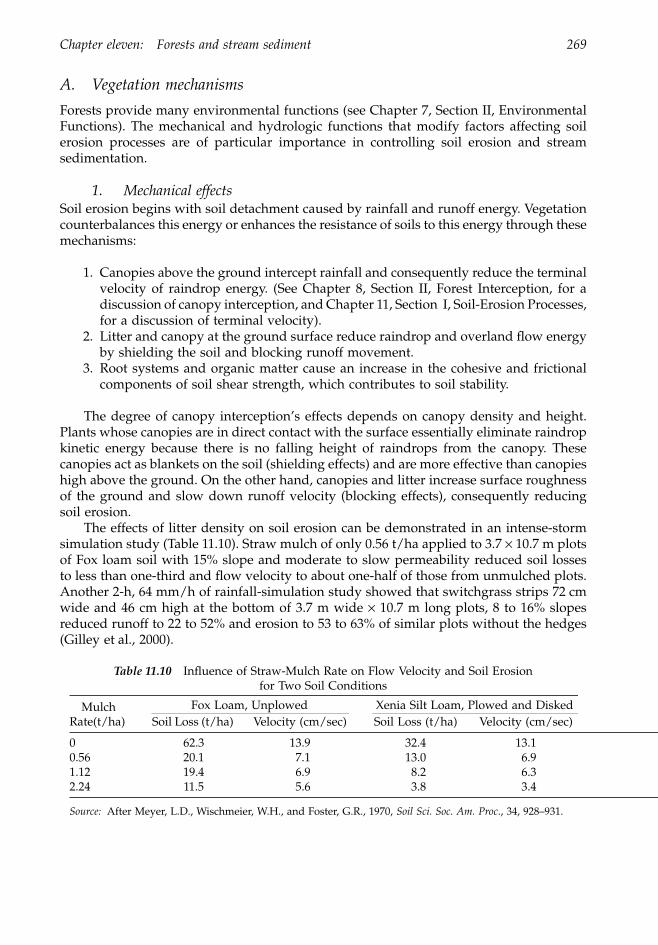
Chapter eleven: Forests and stream sediment 269
A. Vegetation mechanisms
Forests provide many environmental functions (see Chapter 7, Section II, EnvironmentalFunctions). The mechanical and hydrologic functions that modify factors affecting soilerosion processes are of particular importance in controlling soil erosion and streamsedimentation.
1. Mechanical effectsSoil erosion begins with soil detachment caused by rainfall and runoff energy. Vegetationcounterbalances this energy or enhances the resistance of soils to this energy through thesemechanisms:
1. Canopies above the ground intercept rainfall and consequently reduce the terminalvelocity of raindrop energy. (See Chapter 8, Section II, Forest Interception, for adiscussion of canopy interception, and Chapter 11, Section I, Soil-Erosion Processes,for a discussion of terminal velocity).
2. Litter and canopy at the ground surface reduce raindrop and overland flow energyby shielding the soil and blocking runoff movement.
3. Root systems and organic matter cause an increase in the cohesive and frictionalcomponents of soil shear strength, which contributes to soil stability.
The degree of canopy interception’s effects depends on canopy density and height.Plants whose canopies are in direct contact with the surface essentially eliminate raindropkinetic energy because there is no falling height of raindrops from the canopy. Thesecanopies act as blankets on the soil (shielding effects) and are more effective than canopieshigh above the ground. On the other hand, canopies and litter increase surface roughnessof the ground and slow down runoff velocity (blocking effects), consequently reducingsoil erosion.
The effects of litter density on soil erosion can be demonstrated in an intense-stormsimulation study (Table 11.10). Straw mulch of only 0.56 t/ha applied to 3.7 ¥ 10.7 m plotsof Fox loam soil with 15% slope and moderate to slow permeability reduced soil lossesto less than one-third and flow velocity to about one-half of those from unmulched plots.Another 2-h, 64 mm/h of rainfall-simulation study showed that switchgrass strips 72 cmwide and 46 cm high at the bottom of 3.7 m wide ¥ 10.7 m long plots, 8 to 16% slopesreduced runoff to 22 to 52% and erosion to 53 to 63% of similar plots without the hedges(Gilley et al., 2000).
Table 11.10 Influence of Straw-Mulch Rate on Flow Velocity and Soil Erosion for Two Soil Conditions
Mulch Rate(t/ha)
Fox Loam, Unplowed Xenia Silt Loam, Plowed and DiskedSoil Loss (t/ha) Velocity (cm/sec) Soil Loss (t/ha) Velocity (cm/sec)
0 62.3 13.9 32.4 13.10.56 20.1 7.1 13.0 6.91.12 19.4 6.9 8.2 6.32.24 11.5 5.6 3.8 3.4
Source: After Meyer, L.D., Wischmeier, W.H., and Foster, G.R., 1970, Soil Sci. Soc. Am. Proc., 34, 928–931.
1363_C11_fm Page 269 Wednesday, December 4, 2002 7:44 AM
270 Forest Hydrology: An Introduction to Water and Forests
While deep-rooted, woody vegetation is more effective than grass roots for slopestabilization, fine roots of dense grasses and herbaceous vegetation are very beneficial forprotection against raindrop and wind erosion. Large roots penetrate the surface horizonsto anchor the soil mantle to the substrate; fine roots, fungal mycelia, and decomposedorganic matter contribute to the formation of stable aggregates of surface soils. Thesetaproots and lateral roots develop a dense network that interweaves a soil–root systemcentered on the vicinity of individual trees. Soil mantles are thus stabilized due to thegreat reinforcement and binding effects of the soil–root system.
The shear strength of soils against erosion is positively related to root concentration(biomass of roots per unit volume of soil in kg m-3), to root area ratio (the fraction of thetotal cross-sectional area of a soil occupied by roots), and to root tensile strength. Roottensile strengths (the resistance to a force tending to tear roots apart) are about 10 to50 Mpa for most species. They are higher for roots of smaller diameters (more surfacearea), growing uphill, and in late fall (the time of strongest growth), and decline with ageafter tree harvesting. In New Zealand, forest removal often caused landslides on steepslopes along the plane beneath the zone of dense root networks (Sidle et al., 1985).
Generally, conifer roots tend to have a lower tensile strength than deciduous trees,and shrubs appear to have tensile strengths comparable to trees (Gray and Sotir, 1996).This is of particular significance for shallow soils and stream banks where the growth oftrees may accompany an increase in shear stress to the soils due to their greater weightand rigidity. Windthrowing and uprooting of trees in high winds can reduce the stabilityof slopes with shallow soils, streambanks, and levee embankment.
2. Hydrologic effectsThe hydrologic functions of vegetation are very beneficial to the control of soil erosionand stream sediment. They include: (1) interception loss that reduces net precipitationto reach mineral soils, (2) transpiration that depletes soil moisture content, and (3) litterand organic matter that slow down flow velocity and prolong time of concentration. Allthese lead to an increase in infiltration rate and a decrease of sediment-transport capacityin runoff.
Forests reduce erosion and sediment much more than other types of vegetationbecause of greater hydrologic impacts induced by their size and density. In a nationalsurvey of suspended sediment conducted at 63 stations in Kenya during 1948–1968(Dunne, 1977), stream sediment was found to be the lowest in watersheds with greaterforested area. The survey grouped all watersheds into four land-use types: (1) forest, (2)more forest than agriculture, (3) more agriculture than forest, and (4) grazing dominant.Sediment yield (S, t/km2/year) for each land use increases with mean annual runoff (Q,mm) by these relationships:
Forest:
S = 2.670(Q)0.38 (11.52)
Forest > Agriculture:
S = 0.042(Q)1.18 (11.53)
Agriculture > Forest:
S = 0.038(Q)1.41 (11.54)
1363_C11_fm Page 270 Wednesday, December 4, 2002 7:44 AM
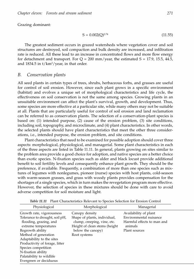
Chapter eleven: Forests and stream sediment 271
Grazing dominant:
S = 0.002(Q)2.74 (11.55)
The greatest sediment occurs in grazed watersheds where vegetation cover and soilstructures are destroyed, soil compaction and bulk density are increased, and infiltrationrate is reduced. All these lead to an increase in concentrated flows and more flow energyfor detachment and transport. For Q = 200 mm/year, the estimated S = 17.9, 15.5, 44.5,and 1834.5 in t/km2/year, in that order.
B. Conservation plants
All seed plants in certain types of trees, shrubs, herbaceous forbs, and grasses are usefulfor control of soil erosion. However, since each plant grows in a specific environment(habitat) and evolves a unique set of morphological characteristics and life cycle, theeffectiveness on soil conservation is not the same among species. Growing plants in anunsuitable environment can affect the plant’s survival, growth, and development. Thus,some species are more effective at a particular site, while many others may not be suitableat all. Plants that are particularly useful for control of soil erosion and land reclamationcan be referred to as conservation plants. The selection of a conservation-plant species isbased on: (1) intended purpose, (2) cause of the erosion problem, (3) site conditions,including soil, topography, and microclimate, and (4) plant characteristics. In other words,the selected plants should have plant characteristics that meet the other three consider-ations, i.e., intended purpose, the erosion problem, and site conditions.
Plant characteristics that need to be examined for possible adoption should cover threeaspects: morphological, physiological, and managerial. Some plant characteristics in eachof the three aspects are listed in Table 11.11. In general, plants growing on sites similar tothe problem area provide a good choice for adoption, and native species are a better choicethan exotic species. N-fixation species such as alder and black locust provide additionalbenefit to soil fertility levels and consequently enhance plant growth. They should be thepreference, if available. Frequently, a combination of more than one species such as mix-tures of legumes with nonlegumes, pioneer (nurse) species with host plants, cold-seasonwith warm-season grasses, and grass with woody plants provides compensation for theshortages of a single species, which in turn makes the revegetation program more effective.However, the selection of species in these mixtures should be done with care to avoidadverse competition for soil moisture and light.
Table 11.11 Plant Characteristics Relevant to Species Selection for Erosion Control
Physiological Morphological Managerial
Growth rate, vigorousness Canopy density Availability of plantTolerance to drought, soil pH, flooding, grazing, and extreme temperatures
Regrowth abilityMethod of generationAdaptability to the sitesProductivity of forage, litterSpecies competitionN-fixation abilityPalatability to wildlifeEvergreen or deciduous
Shape of plants, individual, clump, creeping, vine, etc.
Height of clean stems (height below the canopy)
Root systems
Environmental nuisanceHarmful effects to man and animals
Plant sources
1363_C11_fm Page 271 Wednesday, December 4, 2002 7:44 AM
272 Forest Hydrology: An Introduction to Water and Forests
C. Forest activity
The USLE estimates that interrill and rill erosion for a forested site, as described by theC factor, can be less than for a cleared site by a factor of more than 1000. Any forestactivities that reduce canopy coverage and disturb forest floor and soils will lead to anincrease in gross erosion and sediment yield. The increase in sediment production in aforest activity depends on the degree of forest and soil disturbances.
1. Forest roadsForest roads are recognized as a major source of erosion and can account for as much as90% of all sediment production in forested watersheds (Swift, 1984). This is due to: (1) alow permeability of the road surface, (2) the alteration of natural surface drainage paths,(3) the creation of concentrated overland flow by ditch systems and relief culverts, (4) thesusceptibility of cut-slopes and fill-slopes to soil erosion, and (5) the construction andmaintenance of stream crossings in developing a forest road system. Damaging roadsthat result from water-drainage problems can trigger mass movement (Gucinski et al.,2001). Studies have showed that sediment yield is related to road gradient, surface density,the diameter of materials, slope-length factor, percentage of forest cover over the fill, androad density (EPA, 1975; Burroughs and King, 1985; Campbell and Stednick, 1983; Brakeet al., 1997).
The primary issues in controlling erosion on forest roads are adequate planning,overland runoff management, topography, and revegetation. Runoff diversion from theroad surface or eroding ditch to the forest and a reduction of road gradients are used asprimary practices in existing road systems. In humid Alabama, vegetation treatmentsreduced more than 90% of sediment production and have shown the greatest potentialfor mitigation of soil erosion on forest road side-slopes (Grace, 2000).
2. Forest cutting and site preparationClearcutting followed by mechanical site preparation is a common practice for enhancingforest regeneration in the southern U.S. Because of the intensity of site disturbance,mechanical site preparation caused soil erosion in the first post-treatment year as muchas 12.8 metric t/ha/year in northern Mississippi (Beasley, 1979). The average erosion ratesfor forest harvesting followed by site preparation in the southeast U.S. were estimated torange from 0.05 to 10 t/ha (Table 11.12). A plot study conducted in east Texas showed thatthe sediment production generated from two consecutive storms, a 17.65-cm storm with16-h, 55-min duration followed by a 0.98-cm storm 22 h later, was quite different undersix forest conditions (Table 11.13). Under the full forest cover, sediment production wasonly 1.4 kg/ha, but it increased to 1250 kg/ha for the harvested and sheared plot, 244times higher. The cultivated plot generated 1250 kg/ha sediment, 3.7 times greater thanthe sheared plot.
3. Forest firesThe effects of forest fire, either naturally induced or prescriptively burned, on erosion andsedimentation depend on the frequency and severity of fires, soil conditions, cover type,topography, and weather conditions of the postfire period. Generally, the effects are greaterin the drier West than in the humid East, on fine-textured soils than on sandy soils, forbrush lands than for coniferous forests, and in plantations than in mixed forests. A tre-mendous amount of sediment can be generated if a severe fire that destroys most of thevegetation is followed by high-intensity rainfall. In the Sierra Nevada, a single stormproduced 880 kg/ha of sediment from a 98-ha watershed with vegetation and forest floor
1363_C11_fm Page 272 Wednesday, December 4, 2002 7:44 AM
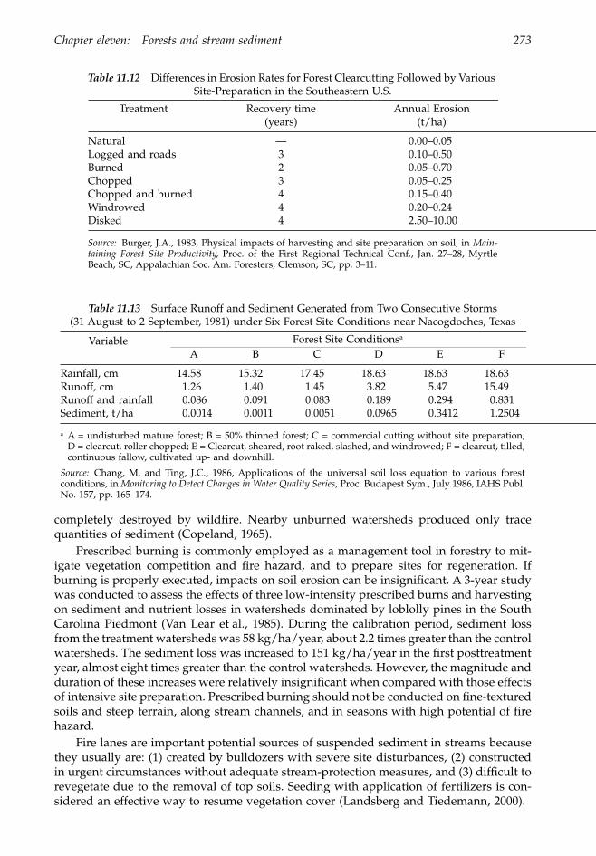
Chapter eleven: Forests and stream sediment 273
completely destroyed by wildfire. Nearby unburned watersheds produced only tracequantities of sediment (Copeland, 1965).
Prescribed burning is commonly employed as a management tool in forestry to mit-igate vegetation competition and fire hazard, and to prepare sites for regeneration. Ifburning is properly executed, impacts on soil erosion can be insignificant. A 3-year studywas conducted to assess the effects of three low-intensity prescribed burns and harvestingon sediment and nutrient losses in watersheds dominated by loblolly pines in the SouthCarolina Piedmont (Van Lear et al., 1985). During the calibration period, sediment lossfrom the treatment watersheds was 58 kg/ha/year, about 2.2 times greater than the controlwatersheds. The sediment loss was increased to 151 kg/ha/year in the first posttreatmentyear, almost eight times greater than the control watersheds. However, the magnitude andduration of these increases were relatively insignificant when compared with those effectsof intensive site preparation. Prescribed burning should not be conducted on fine-texturedsoils and steep terrain, along stream channels, and in seasons with high potential of firehazard.
Fire lanes are important potential sources of suspended sediment in streams becausethey usually are: (1) created by bulldozers with severe site disturbances, (2) constructedin urgent circumstances without adequate stream-protection measures, and (3) difficult torevegetate due to the removal of top soils. Seeding with application of fertilizers is con-sidered an effective way to resume vegetation cover (Landsberg and Tiedemann, 2000).
Table 11.12 Differences in Erosion Rates for Forest Clearcutting Followed by Various Site-Preparation in the Southeastern U.S.
Treatment Recovery time(years)
Annual Erosion (t/ha)
Natural — 0.00–0.05Logged and roads 3 0.10–0.50Burned 2 0.05–0.70Chopped 3 0.05–0.25Chopped and burned 4 0.15–0.40Windrowed 4 0.20–0.24Disked 4 2.50–10.00
Source: Burger, J.A., 1983, Physical impacts of harvesting and site preparation on soil, in Main-taining Forest Site Productivity, Proc. of the First Regional Technical Conf., Jan. 27–28, MyrtleBeach, SC, Appalachian Soc. Am. Foresters, Clemson, SC, pp. 3–11.
Table 11.13 Surface Runoff and Sediment Generated from Two Consecutive Storms (31 August to 2 September, 1981) under Six Forest Site Conditions near Nacogdoches, Texas
Variable Forest Site Conditionsa
A B C D E F
Rainfall, cm 14.58 15.32 17.45 18.63 18.63 18.63Runoff, cm 1.26 1.40 1.45 3.82 5.47 15.49Runoff and rainfall 0.086 0.091 0.083 0.189 0.294 0.831Sediment, t/ha 0.0014 0.0011 0.0051 0.0965 0.3412 1.2504
a A = undisturbed mature forest; B = 50% thinned forest; C = commercial cutting without site preparation;D = clearcut, roller chopped; E = Clearcut, sheared, root raked, slashed, and windrowed; F = clearcut, tilled,continuous fallow, cultivated up- and downhill.
Source: Chang, M. and Ting, J.C., 1986, Applications of the universal soil loss equation to various forestconditions, in Monitoring to Detect Changes in Water Quality Series, Proc. Budapest Sym., July 1986, IAHS Publ.No. 157, pp. 165–174.
1363_C11_fm Page 273 Wednesday, December 4, 2002 7:44 AM
274 Forest Hydrology: An Introduction to Water and Forests
ReferencesAmaranthus, M.O. et al., 1985, Logging and forest roads related to increased debris slides in south-
western Oregon, J. For., 83, 229–233.Anderson, H.W., 1971, Relative contributions of sediment from source areas, and transport processes,
in Proc. Sym. Forest Land Uses and Stream Environment, School of Forestry, Oregon StateUniversity, Corvallis, OR, pp. 55–63.
Arnoldus, H.M.J., 1980, An approximation of the rainfall factor in the USLE, in Assessment of Erosion,DeBoodt, M. and Gabriels, D., Eds., John Wiley & Sons, New York, pp. 127–132.
Bagnold, R.B., 1977, Bed load transport by natural rivers, Water Resour. Res., 13, 303–312.Barry, P.V. et al., 1991, Organic polmers’ effect on soil shear strength and detachment by single
raindrops, Soil Sci. Soc. Am. J., 55, 799–804.Beasley, R.S., 1979, Intensive site preparation and sediment losses on steep watersheds in the Gulf
coastal plain, Soil Sci. Soc. Am. J., 43, 412–417.Beasley, D.B., Huggins, L.F., and Monke, E.J., 1980, ANSWER: a model for watershed planning,
Trans. ASAE, 23, 938–944.Beer, C.E. and Johnson, H.P., 1963, Factors in gully growth in the deep loess area of western Iowa,
Trans. ASAE, 6, 237–240.Bennett, S.J. and Alonso, C.V., 2000, Experiments on headcut growth and migration in concentrated
flows typical of upland areas, Water Resour. Res., 36, 1911–1922.Bennett, S.J. et al., 2000, Characteristics of actively eroding ephemeral gullies in an experimental
channel, Trans. ASAE, 43, 641–649.Bhowimik, N.G. et al., 1980, Hydraulics of Flow and Sediment Transport in the Kankakee River in
Illinois, Illinois State Water Survey, ISWS/RI-98/80.Brake, D., Molnau, M., and King, J.G., 1997, Sediment Transport Distance and Culvert Spacings on
Logging Roads within the Oregon Coast Mountain Range,Paper No. IM-975018, presentedat the 1997 Annual International Meeting, ASAE, Minneapolis, MN, August 10–14.
Bubenzer, G.D. and Jones, B.A., 1971, Drop size and impact velocity effects on the detachment ofsoils under simulated rainfall, Trans. ASAE, 14, 625–628.
Bunte, K., 1996, Analyses of the Temporal Variation of Coarse Bedload Transport and its Grain SizeDistribution, Gen Tech. Rep. RM-GTR-288, USDA Rocky Mountain Forest and Range Exp.Sta., Fort Collins, CO.
Burger, J.A., 1983, Physical impacts of harvesting and site preparation on soil, in Maintaining ForestSite Productivity, Proc. of the First Regional Technical Conf., Jan. 27–28, Myrtle Beach, SC,Appalachian Soc. Am. Foresters, Clemson, SC, pp. 3–11.
Burroughs, E.R., Jr. and King, J.G., 1985. Surface erosion control in roads in granitic soils, in Proc.Sym. Sponsored by Comm. On Watershed Management/Irrigation and Drainage Division, ASCEConvention, April 30-May 1, Denver, CO.
Campbell, D.H. and Stednick, J.D., 1983, Transport of Road Derived Sediment as a Function of SlopeCharacteristics and Time, Final Report (Contract 28-C2–214), USDA Forest Service, RockyMountain Forest and Range Exp. Sta., Ft. Collins, CO.
Chang, M., 1997, Improper soil management causing severe water erosion problems, Proc. Conf.28th, at Nashville, Tenn. on Feb. 25–28, 1997, International Erosion Control Association,pp. 495–501.
Chang, M., Roth, F.A., II, and Hunt, E.V. Jr., 1982, Sediment production under various forest-siteconditions, in Recent Development in the Explanation and Prediction of Erosion and Sediment Yield,Walling, D.E., Ed., IAHS, pp. 13–22.
Chang, M., Sayok, A.K., and Watterston, K.G., 1992, Comparison of three proposed C-values of thesoil loss equation for various forested conditions, in The Environment Is Our Future, Proc.Conf. XXIII, International Erosion Control Assoc., Reno, NV, Feb. 18–21, pp. 241–246.
Chang, M. and Ting, J.C., 1986, Applications of the universal soil loss equation to various forestconditions, in Monitoring to Detect Changes in Water Quality Series, Proc. Budapest Sym., July1986, IAHS Publ. No. 157, pp. 165–174.
Chang, M. and Wong, K.L., 1983, Effects of land use and watershed topography on sediment deliveryratio in East Texas, Beitrage zur Hydrologie, 9, 55–69.
1363_C11_fm Page 274 Wednesday, December 4, 2002 7:44 AM

Chapter eleven: Forests and stream sediment 275
Chapman, G., 1948, Size of raindrops and their striking force at the soil surface in a red pineplantation, Trans. Am. Geophys. Union, 29, 664–70.
Copeland, O.L., Jr., 1965, Land use and ecological factors in relation to sediment yields, in Proc. Fed.Inter-Agency Sedimentation Conf., 1963, USDA Misc. Publ. 970, pp. 72–84.
Cruse, R.M. and Larson, W.E., 1977, Effect of soil shear strength and soil detachment due to raindropimpact, Soil Sci. Soc. Am. J., 41, 777–781.
Dendy, F.E. and Bolton, G.C., 1976, Sediment yield–runoff drainage area relationships in the UnitedStates, J. Soil Water Conserv., 31, 264–266.
Dissmeyer, G.E. and Stump, R.F., 1978, Predicting Erosion Rates for Forest Management Activitiesand Conditions Sample in the Southeast, USDA Forest Service Southeastern Area State andPrivate.
Dunne, T., 1977, Studying patterns of soil erosion in Kenya, FAO Soils Bull., 33, 109–122.Ekern, P.C., 1953, Problems of raindrop impact erosion, Agr. Eng., 34, 23–25, 28.Ellison, W.D., 1944, Studies of raindrop erosion, Agr. Eng., 25, 131–136.EPA, 1975, Logging Roads and Protection of Water Quality, EPA 910/9–75–007.Flaxman, E.M., 1972, Predicting sediment yield in western United States, Proc. Am. Soc. Civ. Eng.
Hydrol. Div., HY12, pp. 2073–2085.Foster, G.R., 1982, Modeling the erosion process, in Hydrologic Modeling of Small Watersheds, Haan,
C.T., Johnson, H.P., and Brakensiek, D.L., Eds., ASAE, St. Joseph, MI, pp. 295–380.Foster, G.R., 1986, Understanding ephemeral gully erosion, in Soil Conservation: Assessing the National
Resources Inventory, Vol. 2, National Academic Press, Washington, D.C., pp. 90–118.Foster, G.R. et al., 1981, Conversion of the universal soil loss equation to SI metric units, J. Soil Water
Conserv., 36, 355–359.Foster, G.R. and Meyer, L.D., 1972, A closed-form soil erosion equation for upland areas. in Sedi-
mentation Sym. To Honor Professor Hans Albert Einstein, Shen, H.W., Ed., Colorado State Uni-versity, Fort Collins, pp. 12.1–12.19.
Foster, G.R. and Meyer, L.D., 1975. Mathematical simulation of upland erosion by fundamentalerosion mechanics, in Present and Prospective Technology for Predicting Sediment Yields andSources, USDA Agr. Res. Service, ARS-S-40, pp. 190–207.
Free, G.R., 1960, Erosion characteristics of rainfall, Agr. Eng., 41, 447–449, 455.Gilley, J.E. et al., 2000, Narrow grass hedge effcts on runoff and soil loss, J. Soil Water Conserv., 55,
190–196.Gordon, N.D., McMahon, T.A., and Finlayson, B.L., 1993, Stream Hydrology, an Introduction for Ecol-
ogists, John Wiley & Sons, New York.Gottschalk, L.C., 1964, Sedimentation. Part I: Reservoir sedimentation, in Handbook of Applied Hy-
drology, Chow, V.T., Ed., McGraw-Hill, New York, pp. 1–34.Grace, J.M., III, 2000, Forest road sideslopes and soil conservation techniques, J. Soil Water Conserv.,
55, 96–101.Gray, D.H. and Megahan, W.F., 1981, Forest Vegetation Removal and Slope Stability in the Idaho
Batholith, U.S. Forest Service, Intermountain Forest and Range Exp. Sta., Res. Paper INT-271,Ogden, UT.
Gray, D.H. and Sotir, R.B., 1996, Biotechnical and Soil Bioengineering Slope Stabilization, John Wiley &Sons, New York.
Gucinski, H. et al., 2001, Forest Roads: A Synthesis of Scientific Information, Gen. Tech. Rep. PNW-GTR-509, U.S. Forest Service, Pacific NW Res. Sta., Portland, OR.
Heede, B.H., 1975, Watershed indicators of landform development, in Proc. Hydrol. Water Resour. inArizona and the Southwest, Vol. 5, Arizona Sect. Am. Water Resour. Assoc. Hydro. Sect. ArizonaAcad. Sci., pp. 43–46.
Heede, B.H., 1976, Gully Development and Control: The Status of Our Knowledge, U.S. ForestService, Rocky Mountain Forest and Range Experiment Station, Fort Collins, CO.
Heede, B.H., 1978, Designing gully control systems for eroding watersheds, Environ. Manage., 2,509–522.
Hjulstrom, F., 1939, Transportation: transportation of detritus by moving water, in Sym. Recent MarineSediments, Trask, P.D., Ed., Am. Assoc. Petroleum Geologists, Tulsa, OK, pp. 5–31.
1363_C11_fm Page 275 Wednesday, December 4, 2002 7:44 AM

276 Forest Hydrology: An Introduction to Water and Forests
Hudson, N., 1995, Soil Conservation, Iowa State University Press, Ames, IA.Knisel, W.G., 1980, CREAMS: a Field Scale Model for Chemicals, Runoff, and Erosion from Agri-
cultural Management Systems, Conservation Res. Rep. No. 26., USDA.Laflen, J.M., 1986, Ephemeral gully erosion, in Proc. Fourth Federal Interagency Sediment Conference,
March 24–27, 1986, Las Vegas, NV, Vol. I, Sec. 3, pp. 29–37.Lal, R., Ed., 1994, Soil Erosion Research Methods, Soil Water Conserv. Soc., Ankeny, IA.Lal, R. and Elliot, W.,1994, Erodibility and erosivity, in Soil Erosion Research Methods, Lal, R., Ed., Soil
Water Conserv. Soc., Ankeny, IA, pp. 181–208.Landsberg, J.D. and Tiedemann, A.R., 2000, Fire management, in Drinking Water from Forests and
Grasslands, a Synthesis of the Scientific Literature, G.E. Dissmeyer, Ed., Gen. Tech. Rep. SRS39,USDA Forest Service, Southern Research Station.
Lane, L.J., 1982, Development of a procedure to estimate runoff and sediment transport in ephemeralstreams, in Recent Developments in the Explanation and Prediction of Erosion and Sediment Yield,Walling, D.E., Ed., IAHS, pp. 275–282.
Laursen, E.M., 1958, Sediment transport mechanics in stable channel designs, Trans. ASCE, 123,195–206.
Laws, J.O. and Parsons, D.A., 1943, The relation of raindrop size to intensity, Trans. Am. Geophys.Union, 24, 452–459.
Laws, J.O., 1941, Trans Am. Geophys. Union, 22, 709–721.Lo, A. et al., 1985, Effectiveness of EI30 as an erosivity index in Hawaii, in Soil Erosion and Conservation,
El-Swaify, S.A., Moldenhauer, W.C., and Lo, A., Eds., Soil Conserv. Soc. Am., Ankeny, IA.,pp. 384–392.
Lyles, L., 1977, Soil detachment and aggregate disintegration by wind-driven rain, in Soil Erosion:Prediction and Control, Soil Conserv. Soc. Am., Ankeny, IA, pp. 152–159.
Magahan, W.F., Day, N.F., and Bliss, T.M., 1978, Landslide occurrences in the western and centralnorthern Rocky Mountain physiographic province in Idaho, The 5th North Amer. Forest SoilsConf., Colorado State University, Fort Collins, pp. 116–139.
Maner, S.B., 1962, Factors Influencing Sediment Delivery Ratios in the Blackland Prairie LandResource Area, USDA, Soil Conservation Service, Fort Worth, TX.
Martinzer, M.R., Fogel, M.M., and Lane, L.J. , 1980, Modeling for Upland Areas, Paper No. 80–2505,Am. Soc. Agr. Eng., St. Joseph, MI.
McGregor, K.C. and Mutchler, C.K., 1977, Status of the R factor in northern Mississippi, in SoilErosion: Prediction and Control, Soil Conserv. Soc. Am., Ankeny, IW, pp. 135–142.
Merkel, W.H., Woodward, D.W., and Clarke, C.D., 1988, Ephemeral gully erosion model (EGEM),in Model Agricultural, Forest, and Rangeland Hydrology, Proc. of the 1988 Int. Sym., ASAE,St. Joseph, MI, pp. 315–322.
Meyer, L.D., 1981, How rain intensity affects interrill erosion, Trans. ASAE, 24, 1472–1475.Meyer, L.D. and Harmon, W.C., 1984, Susceptibility of agricultural soils to interrill erosion, Soil Sci.
Soc. Am. J., 48, 1152–1157.Meyer, L.D. and Wischmeier, W.H., 1969, Mathematical simulation of the process of soil erosion by
water, Trans. ASAE, 12, 754–758, 762.After Meyer, L.D., Wischmeier, W.H., and Foster, G.R., 1970, Soil Sci. Soc. Am. Proc., 34, 928–931.Morgan, R.P.C., 1986, Soil Erosion and Conservation, Longman Scientific & Technical, Hong Kong.Musgrave, G.W., 1947, The quantitative evaluation of factors in water erosion: a first approximation,
J. Soil Water Conserv., 2, 133–138.Mutchler, C.K. and Bowie, A.J., 1976, Effect of land use on sediment delivery ratios, Proc. of the Third
Fed. Inter-Agency Sedimentation Conf., Denver, CO, pp. I:11–I:21.Nearing, M.A., Lane, L.J., and Lopes, V.L., 1994, Modeling soil erosion, in Soil Erosion Research
Methods, Lal, R., Ed., Soil Water Conserv. Soc., Ankeny, IA, pp. 127–156.Parker, J.C., Amos, D.F., and Sture,, S., 1980, Measurements of swelling, hydraulic conductivity, and
shear strength in a multistage triaxial test, Soil Sci. Soc. Am. J., 44, 1133–1138.Piest, R.F., Bradford, J.M., and Spomer, R.G., 1975, Mechanisms of erosion and sediment movement
from gullies. in Present and Prospective Technology for Predicting Sediment Yields and Resources,USDA, Agr. Res. Sev., ARS-S-40, pp. 162–176.
1363_C11_fm Page 276 Wednesday, December 4, 2002 7:44 AM
Chapter eleven: Forests and stream sediment 277
Renald, K.G., 1980, Estimating erosion and sediment yield from rangeland, in Sym. Watershed Man-agement 1980, Vol. l, ASAE, New York, pp. 164–175.
Renard, K.G. et al., 1997, Predicting Soil Erosion by Water: A Guide to Conservation Planning with theRevised Universal Soil Loss Equation (RUSLE), USDA-ARS Agricultural Handbook No. 703.
Renard, K.G. et al., 1991, RUSLE: revised universal soil loss equation, J. Soil Water Conserv., 46, 30–33.Renard, K.G. and Freimund, J.R., 1994, Using monthly precipitation data to estimate the R-factor in
the revised USLE, J. Hydrology, 157, 287–306.Renard, K.G. et al., 1994, The revised universal soil loss equation, in Soil Erosion Research Methods,
2nd Ed., Lal, R., Ed., Soil Water Conserv. Soc., Ankeny, IA, pp. 105–124.Renfro, G.W., 1975, Use of erosion equations and sediment delivery ratios for predicting sediment
yield, in Proc. of Sediment-Yield Workshop on Present and Prospective Tech. for Predicting SedimentYields and Sources, USDA, ARS-40, pp. 33–45.
Robinson, K.M. and Hanson, G.J., 1996, Gully headcut advance, Am. Soc. Agr. Eng., 39, 33–38.Roehl, J.E., 1962, Sediment Source Areas, Delivery Ratios and Influencing Morphological Factors,
International Assoc. Hydro. Sci., Publ. No. 59, pp. 202–213.Roose, E., 1977, Erosion et Ruisselement en Afrique de l’ouest — vingt annees de measures en petites
parcelles esperimentales, Travaux et Documenys de l’ORSTOM No. 78, ORSTOM, Paris.Rosgen, D.L., Knapp, K.L., and Megahan, W.F., 1980, Total potential sediment, in An Approach to
Water Resources Evaluation of Non-Point Silvicultural Sources (A Procedural Handbook), EPA-600/8–80–012, U.S. Environ. Protection Agency, pp. Vl.1–43.
Shields, N.D., 1936, Anwendung der Ahnlichkeit Mechanik und der Turbulenzforschung auf dieGeschiebelerwegung, Mitt. Preoss Versuchanstalt für Wasserbau und Schiffau, 26.
Sidle, R.C., Pearce, A.J., and O’Loughlin, C.L., 1985, Hillslope Stability and Land Use, Am. Geophy.Union, Water Resour. Monog. Series 11.
Simanton, J.R. and Renard, K.G., 1982, The USLE rainfall factor for southwest U.S. Rangelands. inProc. Workshop on Estimating Erosion and Sediment Yield from Rangelands, USDR-ARS Agr.Reviews and Manuals, ARS-W-26, Tucson, AZ, pp. 50–62.
Swift, L.W., Jr., 1984, Soil losses from roadbeds and cut and fill slopes in the southern AppalachianMountains, South. Appl. For., 8, 209–215.
Thompson, J.R., 1964, Quantitative effect of watershed variables on rate of gully-head advancement,Trans. ASAE, 7, 54–55.
Thorne, C.R. and Zevenbergen, W., 1990, Prediction of ephemeral gully erosion on cropland in thesoutheastern United States, in Soil Erosion on Agricultural Land, Boardman, J., Foster, I.D.L.,and Dearing, J.A., Eds., John Wiley & Sons, New York, pp. 447–460.
Truman, C.C. et al., 2001, Slope length effects on runoff and sediment delivery, J. Soil Water Conserv.,56, 249–256.
USDA, 1995, USDA Water Erosion Prediction Project (WEPP), User Summary, NSERL Rep. No. 11,USDA-ARS-MWA, National Soil Erosion Research Laboratory, West Lafayette, IN.
UNESCO, 1982, Sedimentation problems in river basins, Proj. 5.3 of the International HydrologicalProgramme, United Nations Edu. Sci. and Cultural Organ, Paris.
UNESCO, 1991, The Water-Related Issues and Problems of the Humid Tropics and Other Warm HumidRegions: A Programme for the Humid Tropics, Division of Water Sciences, UNESCO. Paris.
U.S. Soil Conservation Service, 1977, Procedure for determining rates of land damage, land depre-ciation and volume of sediment produced by gully erosion, in Guidelines for Watershed Man-agement, FAO, Rome, pp. 125–142.
Van Lear, D.H. et al., 1985, Sediment and nutrient export in runoff from burned and harvested pinewatersheds in the South Carolina Piedmont, J. Environ. Qual, 24, 169–174.
Walling, D.E., 1974, Suspended sediment and solute yields from a small catchment prior to urban-ization, in Fluvial Processes in Instrumented Watersheds, Gregory. K.J. and Walling, D.E., Eds.,Institute of British Geographers, London, pp. 169–192.
Walling, D.E., 1994, Measuring sediment yield from river basins, in Soil Erosion Research Methods,Lal. R., Ed., Soil Water Conserv. Soc., Ankeny, IA, pp. 39–80.
Watson, D.A., Laflen, J.M., and Franti, T.G., 1986, Estimating Ephemeral Gully Erosion, Paper No.86–2020, Summer Meeting, ASAE. St. Joseph, MI.
1363_C11_fm Page 277 Wednesday, December 4, 2002 7:44 AM
278 Forest Hydrology: An Introduction to Water and Forests
Williams, J.R., 1975, Sediment-yield prediction with universal equation using runoff energy factorin Present and Prospective Technology for Predicting Sediment Yields and Sources, U.S. Agr. Res.Ser., ARS-S-40, pp. 244–252.
William, J.R., 1977, Sediment delivery ratios determined with sediment and runoff models, in Erosionand Solid Matter Transport in Inland Waters, IAHS Publ. No. 122, Willingford, England.pp. 168–179.
Williams, J.R., Renard, K.G., and Dyke, P.T., 1983, A new method for assessing the effect of erosionon predictability — the EPIC model, J. Soil Water Conserv., 38, 381–383.
Wischmeier, W.H. and Smith, D.D., 1958, Rainful energy and its relationship to soil loss, Trans. Am.Geophy. Union, 39, 285–291.
Wischmeier, W.H., 1975, Estimating the soil loss equation’s cover and management factor for un-disturbed areas, in Present and Prospective Technology for Predicting Sediment Yields and Sources,USDA Agr. Res. Service, ARS-S-40, pp. 118–124.
Wischmeier, W.H. and Smith, D.D., 1978, Predicting Rainfall Erosion Losses, a Guide to ConservationPlanning, USDA Agr. Handbook No. 537.
Woodward, D.E., 1999, Method to predict cropland ephemeral gully erosion, CATENA, 37, 393–399.Yang, C.T., 1972, Unit stream power and sediment transport, J. Hydrau. Div. Am. Soc. Civil Eng., 98,
1805–1827.Young, R.A., and Wiersma, J.L., 1973, The role of rainfall impact in soil detachment and transport,
Water Resour. Res., 9, 1629–1636.Zingg, A.W., 1940, Degree and length of land slopes as it affects soil loss in runoff, Agr. Eng., 21, 59–64.
1363_C11_fm Page 278 Wednesday, December 4, 2002 7:44 AM

279
chapter twelve
Research in forest hydrology
Contents
I. Research issues ................................................................................................................281A. Objectives .................................................................................................................281
1. Cause and effect................................................................................................2812. Prediction ...........................................................................................................2813. Management ......................................................................................................282
B. Subjects .....................................................................................................................2821. Water functions .................................................................................................2822. Forest functions.................................................................................................2823. Watershed functions.........................................................................................282
II. Principles of field studies ..............................................................................................283A. Control ......................................................................................................................283B. Randomness.............................................................................................................283C. Replication ...............................................................................................................283
III. Research methods ...........................................................................................................284A. Experimental watersheds ......................................................................................284
1. Paired-watershed approach ............................................................................284a. Watershed selections ..................................................................................284b. Calibration methods...................................................................................285c. Treatment methods .....................................................................................286d. Duration of calibration and treatment periods......................................286e. Treatment effects .........................................................................................288f. Criticisms of the approach ........................................................................289
2. Single-watershed approach.............................................................................2893. Replicated-watershed approach .....................................................................290
B. Upstream–downstream approach........................................................................291C. Experimental plots..................................................................................................291D. Regional analysis ....................................................................................................292E. Watershed simulation ............................................................................................293
IV. Example of calibration and analyses: the Wagon Wheel Gap study .....................295A. Hydroclimatic data .................................................................................................295B. The calibration equation........................................................................................296C. Assessment of treatment effects ...........................................................................296
1. How much effect?.............................................................................................296a. Preliminary assessment .............................................................................297b. Based on the calibration equation............................................................298
1363_C12_fm Page 279 Wednesday, December 4, 2002 7:45 AM
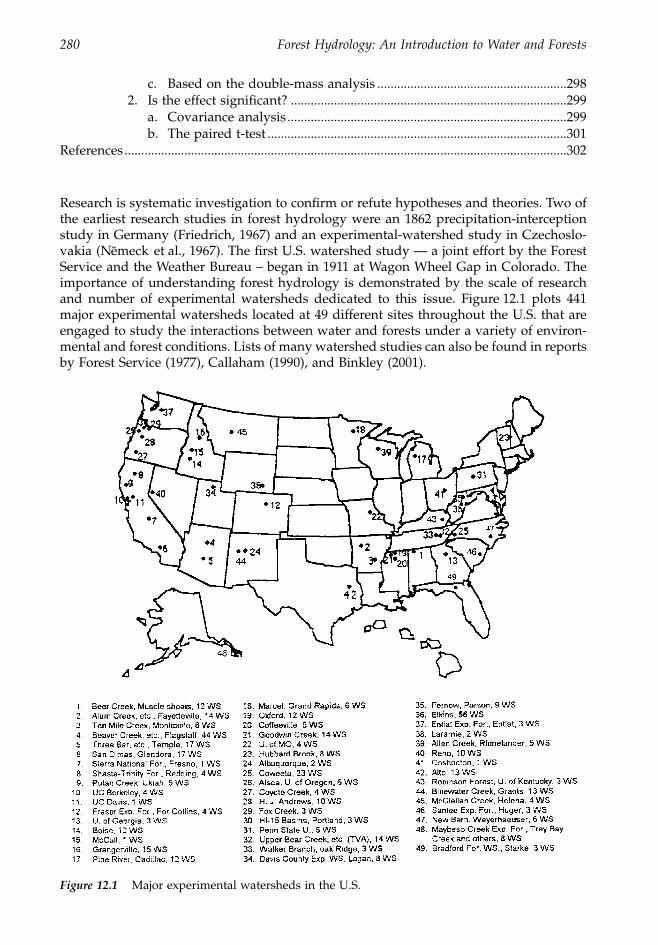
280 Forest Hydrology: An Introduction to Water and Forests
c. Based on the double-mass analysis .........................................................2982. Is the effect significant? ...................................................................................299
a. Covariance analysis ....................................................................................299b. The paired t-test ..........................................................................................301
References .....................................................................................................................................302
Research is systematic investigation to confirm or refute hypotheses and theories. Two ofthe earliest research studies in forest hydrology were an 1862 precipitation-interceptionstudy in Germany (Friedrich, 1967) and an experimental-watershed study in Czechoslo-vakia (Nemeck et al., 1967). The first U.S. watershed study — a joint effort by the ForestService and the Weather Bureau – began in 1911 at Wagon Wheel Gap in Colorado. Theimportance of understanding forest hydrology is demonstrated by the scale of researchand number of experimental watersheds dedicated to this issue. Figure 12.1 plots 441major experimental watersheds located at 49 different sites throughout the U.S. that areengaged to study the interactions between water and forests under a variety of environ-mental and forest conditions. Lists of many watershed studies can also be found in reportsby Forest Service (1977), Callaham (1990), and Binkley (2001).
Figure 12.1
Major experimental watersheds in the U.S.
1363_C12_fm Page 280 Wednesday, December 4, 2002 7:45 AM
Chapter twelve: Research in forest hydrology 281
I. Research issues
Forest hydrology is a pure as well as an applied science and therefore consists of bothbasic and applied types of research. An example of basic research might be a study ofhow channel roughness influences average streamflow velocities. An example of appliedresearch might be a study of how large-wood removal from channels during harvestingaffects peak flows. Yet, the results of the basic research and a hypothesis derived fromthem can be used to explain the expected peakflow-response found in the applied research.Similarly, the results from the applied research can be used to confirm the patterns pre-dicted by the basic understanding of watershed processes. Forest-hydrology researchcontinues to refine our understanding of water in forests.
Issues in forest-hydrology studies can be discussed in terms of research objectives orresearch subjects. Research objectives can be separated into three categories: (1) cause andeffect of plant–water–watershed relationships, (2) predictions of hydrologic consequencescaused by changes in weather conditions, in vegetation communities, or in man’s activities,and (3) management of watershed natural resources and hydrological conditions to serveman’s best interests and needs. Subject issues can also be separated into three categories:(1) water functions, (2) forest functions, and (3) watershed functions.
A. Objectives
1. Cause and effect
Cause-and-effect studies are the fundamental studies in forest hydrology. The objectivesof cause-and-effect studies are to comprehend the hydrological cycle in forested water-sheds, to explain variations in hydrological phenomena among watersheds, and to findphysical laws that govern forest–water–climate–soil–topography relationships (Douglas,1967; Haupt, 1979; Riekerk, 1989; Keppeler and Ziemer, 1990; Ursic, 1991a). Studies forthese purposes may involve evaluations of watershed water-balances, energy budgets,runoff processes, rainfall–runoff relationships, roles of forests in the hydrological cycle,topographic effects, soil-water movements, etc. They require long-term watershed obser-vations over a wide range of environmental conditions. Such requirements are intendedto explain the effects of temporal and spatial variations, and to avoid biased interpretationsthat are due to unrepresentative data.
2. Prediction
Prediction is a major task of all sciences. Based on knowledge learned in cause-and-effectstudies, many studies are conducted to develop methodology and models for predictingconsequences induced under various management activities and environmental condi-tions. In the forest–water interface, those predictions include evaporation from soil andwater (Idso et al., 1979; Penman, 1956; Shuttleworth, 1993), forest transpiration (Stewart,1984), evapotranspiration (Abtew, 1996), interception loss (Massman, 1983), effects of landuse on runoff generation (Douglas, 1983), climate changes and water resources (Cooteret al., 1993; McNulty et al., 1997), snow accumulation and snowmelt (Rango and Martinec,1995; Stegman, 1996), sediment movement and yields (Clayton and Megahan, 1997),nutrient transport (Bakke and Pyles, 1997), and other events. The developed models mustbe calibrated, tested, and validated using data observed in experimental watersheds (Lee,1970; Galbraith, 1975).
Predictions provide a basis for management, control, and adjustment. Besides on-siteand downstream effects, forest and land activities can have impacts upslope as well(Chang, 1997). Up-site, on-site, and down-site impacts should all be considered in predic-tion studies.
1363_C12_fm Page 281 Wednesday, December 4, 2002 7:45 AM
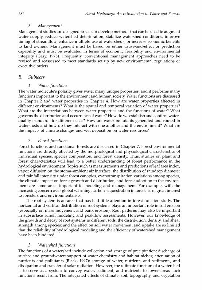
282 Forest Hydrology: An Introduction to Water and Forests
3. Management
Management studies are designed to seek or develop methods that can be used to augmentwater supply, reduce watershed deterioration, stabilize watershed conditions, improvetiming of streamflow, enhance multiple use of watersheds, or increase economic benefitsto land owners. Management must be based on either cause-and-effect or predictioncapability and must be evaluated in terms of economic feasibility and environmentalintegrity (Gary, 1975). Frequently, conventional management approaches need to berevised and reassessed to meet standards set up by new environmental regulations orexecutive orders.
B. Subjects
1. Water functions
The water molecule’s polarity gives water many unique properties, and it performs manyfunctions important to the environment and human society. Water functions are discussedin Chapter 2 and water properties in Chapter 4. How are water properties affected indifferent environments? What is the spatial and temporal variation of water properties?What are the interrelations between water properties and the functions of water? Whatgoverns the distribution and occurrence of water? How do we establish and confirm water-quality standards for different uses? How are water pollutants generated and routed inwatersheds and how do they interact with one another and the environment? What arethe impacts of climate changes and wet deposition on water resources?
2. Forest functions
Forest functions and functional forests are discussed in Chapter 7. Forest environmentalfunctions are directly affected by the morphological and physiological characteristics ofindividual species, species composition, and forest density. Thus, studies on plant andforest characteristics will lead to a better understanding of forest performance in thehydrological environment. Topics such as measurements and predictions of leaf area index,vapor diffusion on the stoma–ambient air interface, the distribution of raindrop diameterand rainfall intensity under forest canopies, evapotranspiration variations among species,the climatic impact on forest growth and distribution, and forest adoption to the environ-ment are some areas important to modeling and management. For example, with theincreasing concern over global warming, carbon sequestration in forests is of great interestto foresters and environmentalists.
The root system is an area that has had little attention in forest function study. Thehorizontal and vertical distribution of root systems plays an important role in soil erosion(especially on mass movement and bank erosion). Root patterns may also be importantin subsurface runoff modeling and peakflow assessments. However, our knowledge ofthe growth and decay of root systems in different soils; the distribution, density, and shearstrength among species; and the effect on soil water movement and uptake are so limitedthat the reliability of hydrological modeling and the efficiency of watershed managementhave been hindered.
3. Watershed functions
The functions of a watershed include collection and storage of precipitation; discharge ofsurface and groundwater; support of water chemistry and habitat niches; attenuation ofnutrients and pollutants (Black, 1997); storage of water, nutrients and sediments; anddissipation and transfer of solar radiation. However, the ultimate function of a watershedis to serve as a system to convey water, sediment, and nutrients to lower areas suchfunctions result from. The integrated effects of climate, soil, topography, and vegetation
1363_C12_fm Page 282 Wednesday, December 4, 2002 7:45 AM
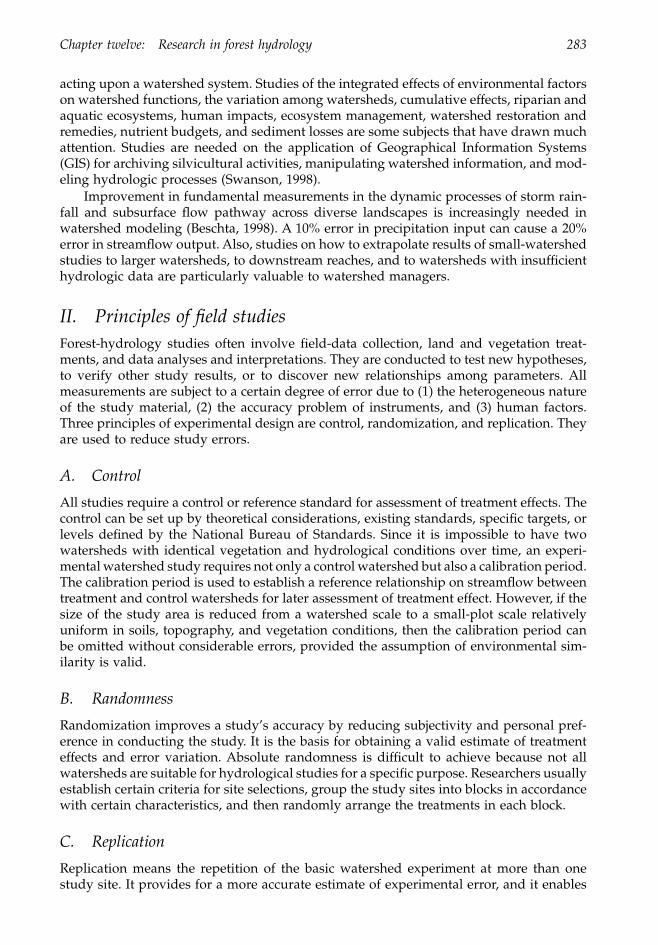
Chapter twelve: Research in forest hydrology 283
acting upon a watershed system. Studies of the integrated effects of environmental factorson watershed functions, the variation among watersheds, cumulative effects, riparian andaquatic ecosystems, human impacts, ecosystem management, watershed restoration andremedies, nutrient budgets, and sediment losses are some subjects that have drawn muchattention. Studies are needed on the application of Geographical Information Systems(GIS) for archiving silvicultural activities, manipulating watershed information, and mod-eling hydrologic processes (Swanson, 1998).
Improvement in fundamental measurements in the dynamic processes of storm rain-fall and subsurface flow pathway across diverse landscapes is increasingly needed inwatershed modeling (Beschta, 1998). A 10% error in precipitation input can cause a 20%error in streamflow output. Also, studies on how to extrapolate results of small-watershedstudies to larger watersheds, to downstream reaches, and to watersheds with insufficienthydrologic data are particularly valuable to watershed managers.
II. Principles of field studies
Forest-hydrology studies often involve field-data collection, land and vegetation treat-ments, and data analyses and interpretations. They are conducted to test new hypotheses,to verify other study results, or to discover new relationships among parameters. Allmeasurements are subject to a certain degree of error due to (1) the heterogeneous natureof the study material, (2) the accuracy problem of instruments, and (3) human factors.Three principles of experimental design are control, randomization, and replication. Theyare used to reduce study errors.
A. Control
All studies require a control or reference standard for assessment of treatment effects. Thecontrol can be set up by theoretical considerations, existing standards, specific targets, orlevels defined by the National Bureau of Standards. Since it is impossible to have twowatersheds with identical vegetation and hydrological conditions over time, an experi-mental watershed study requires not only a control watershed but also a calibration period.The calibration period is used to establish a reference relationship on streamflow betweentreatment and control watersheds for later assessment of treatment effect. However, if thesize of the study area is reduced from a watershed scale to a small-plot scale relativelyuniform in soils, topography, and vegetation conditions, then the calibration period canbe omitted without considerable errors, provided the assumption of environmental sim-ilarity is valid.
B. Randomness
Randomization improves a study’s accuracy by reducing subjectivity and personal pref-erence in conducting the study. It is the basis for obtaining a valid estimate of treatmenteffects and error variation. Absolute randomness is difficult to achieve because not allwatersheds are suitable for hydrological studies for a specific purpose. Researchers usuallyestablish certain criteria for site selections, group the study sites into blocks in accordancewith certain characteristics, and then randomly arrange the treatments in each block.
C. Replication
Replication means the repetition of the basic watershed experiment at more than onestudy site. It provides for a more accurate estimate of experimental error, and it enables
1363_C12_fm Page 283 Wednesday, December 4, 2002 7:45 AM
284 Forest Hydrology: An Introduction to Water and Forests
researchers to obtain a more precise estimate of the mean effect of the study (Ostle andMalone, 1988). Usually three or four replicas are used to cover sample variations; thesereplicas are randomized to avoid any subjectivity. Replication also makes the collecteddata more representative. The entire study may need to be repeated by other researchersto validate the results, and to be tested in different climatic conditions to assess itsapplicability.
III. Research methods
Numerous studies have been conducted to investigate the forest–water yield relationship.The methods employed can be grouped into five categories: (1) experimental watersheds,(2) upstream-downstream approach, (3) experimental plots, (4) regional analysis, and (5)watershed simulation. Experimental watersheds, including the paired-, single-, and rep-licated-watershed approaches, are referred to as the hydrometric method, while experi-mental plots are referred to as the gravimetric method. Regional analysis and watershedsimulation are known as the statistical (empirical) and physical methods, respectively.
A. Experimental watersheds
In this method, one or multiple representative watersheds are selected to study hydrolog-ical processes utilizing streamflow-gaging stations and other hydro-climatic instruments.It has been employed as a principal means of monitoring baseline data on long-termhydro-climatological phenomena, evaluating hydrological impact of various land usesand management activities, and serving as databases for calibrations and validations ofhydrological or ecological models. There are three approaches: paired-watershed, single-watershed, and replicated watersheds.
1. Paired-watershed approach
The paired-watershed approach chooses two or more watersheds to be gaged for study.One of them is designated as the control watershed and the other(s) as the treatmentwatershed(s). The whole study is divided into two periods, a calibration period and atreatment period. The purpose of the calibration period is to establish a reliable hydro-logical relationship (calibration equations) between the control and treatment watershedsthrough statistical analysis. It is used as a reference base to assess treatment effects onstreamflow in the treatment watersheds during the treatment period. After each pair ofwatersheds is satisfactorily calibrated, then the treatment watershed is treated as desig-nated. The treatment effects are calculated between the predicted (from the calibrationequation) and observed values and are evaluated for significance through statistical tests.Details are discussed below.
a. Watershed selections.
All watersheds selected for the study must be represen-tative of the region in question so that the results are transferable to ungaged watersheds.Also, the paired watersheds must be close to each other to ensure similarity with respectto vegetation cover, soil types, topographic characteristics, and climatic conditions. Sinceenvironmental variability is much greater in watersheds of large size and the hydrologicalbehaviors of large watersheds are much different from those of small watersheds, it isimportant that the control and treatment watersheds be comparable in size. Watershedswith potential water leakage due to geological structures should not be used in the study.Valid results are based upon the assumption that all runoff (surface and subsurface) mergesat the gaging stations.
1363_C12_fm Page 284 Wednesday, December 4, 2002 7:45 AM
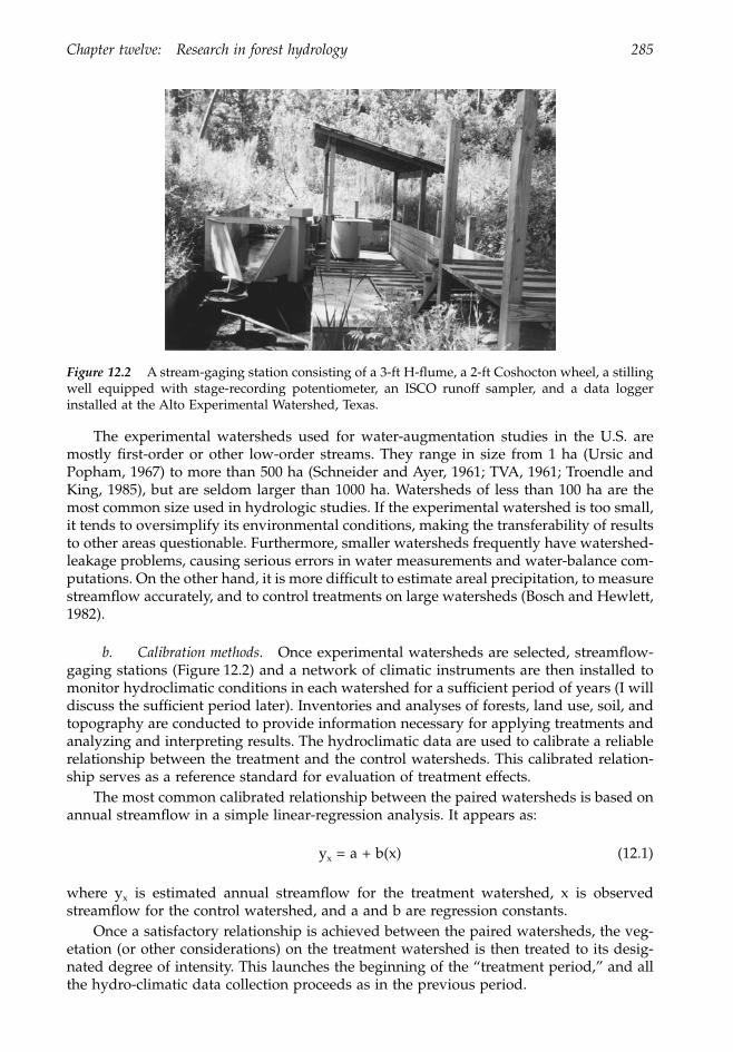
Chapter twelve: Research in forest hydrology 285
The experimental watersheds used for water-augmentation studies in the U.S. aremostly first-order or other low-order streams. They range in size from 1 ha (Ursic andPopham, 1967) to more than 500 ha (Schneider and Ayer, 1961; TVA, 1961; Troendle andKing, 1985), but are seldom larger than 1000 ha. Watersheds of less than 100 ha are themost common size used in hydrologic studies. If the experimental watershed is too small,it tends to oversimplify its environmental conditions, making the transferability of resultsto other areas questionable. Furthermore, smaller watersheds frequently have watershed-leakage problems, causing serious errors in water measurements and water-balance com-putations. On the other hand, it is more difficult to estimate areal precipitation, to measurestreamflow accurately, and to control treatments on large watersheds (Bosch and Hewlett,1982).
b. Calibration methods.
Once experimental watersheds are selected, streamflow-gaging stations (Figure 12.2) and a network of climatic instruments are then installed tomonitor hydroclimatic conditions in each watershed for a sufficient period of years (I willdiscuss the sufficient period later). Inventories and analyses of forests, land use, soil, andtopography are conducted to provide information necessary for applying treatments andanalyzing and interpreting results. The hydroclimatic data are used to calibrate a reliablerelationship between the treatment and the control watersheds. This calibrated relation-ship serves as a reference standard for evaluation of treatment effects.
The most common calibrated relationship between the paired watersheds is based onannual streamflow in a simple linear-regression analysis. It appears as:
y
x
= a + b(x) (12.1)
where y
x
is estimated annual streamflow for the treatment watershed, x is observedstreamflow for the control watershed, and a and b are regression constants.
Once a satisfactory relationship is achieved between the paired watersheds, the veg-etation (or other considerations) on the treatment watershed is then treated to its desig-nated degree of intensity. This launches the beginning of the “treatment period,” and allthe hydro-climatic data collection proceeds as in the previous period.
Figure 12.2
A stream-gaging station consisting of a 3-ft H-flume, a 2-ft Coshocton wheel, a stillingwell equipped with stage-recording potentiometer, an ISCO runoff sampler, and a data loggerinstalled at the Alto Experimental Watershed, Texas.
1363_C12_fm Page 285 Wednesday, December 4, 2002 7:45 AM
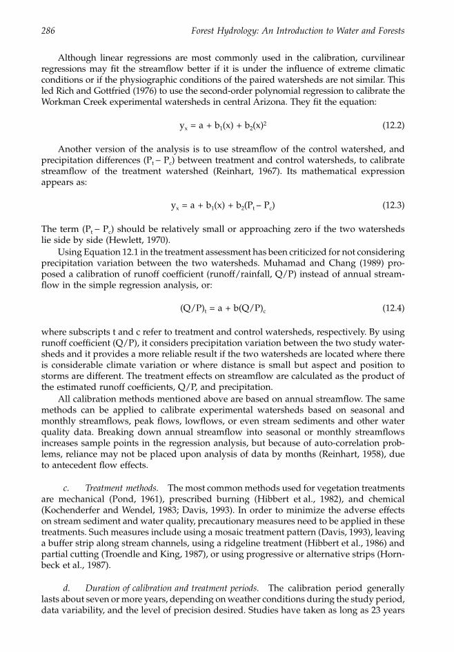
286 Forest Hydrology: An Introduction to Water and Forests
Although linear regressions are most commonly used in the calibration, curvilinearregressions may fit the streamflow better if it is under the influence of extreme climaticconditions or if the physiographic conditions of the paired watersheds are not similar. Thisled Rich and Gottfried (1976) to use the second-order polynomial regression to calibrate theWorkman Creek experimental watersheds in central Arizona. They fit the equation:
y
x
= a + b
1
(x) + b
2
(x)
2
(12.2)
Another version of the analysis is to use streamflow of the control watershed, andprecipitation differences (P
t
-
P
c
) between treatment and control watersheds, to calibratestreamflow of the treatment watershed (Reinhart, 1967). Its mathematical expressionappears as:
y
x
= a + b
1
(x) + b
2
(P
t
– P
c
) (12.3)
The term (P
t
-
P
c
) should be relatively small or approaching zero if the two watershedslie side by side (Hewlett, 1970).
Using Equation 12.1 in the treatment assessment has been criticized for not consideringprecipitation variation between the two watersheds. Muhamad and Chang (1989) pro-posed a calibration of runoff coefficient (runoff/rainfall, Q/P) instead of annual stream-flow in the simple regression analysis, or:
(Q/P)
t
= a + b(Q/P)
c
(12.4)
where subscripts t and c refer to treatment and control watersheds, respectively. By usingrunoff coefficient (Q/P), it considers precipitation variation between the two study water-sheds and it provides a more reliable result if the two watersheds are located where thereis considerable climate variation or where distance is small but aspect and position tostorms are different. The treatment effects on streamflow are calculated as the product ofthe estimated runoff coefficients, Q/P, and precipitation.
All calibration methods mentioned above are based on annual streamflow. The samemethods can be applied to calibrate experimental watersheds based on seasonal andmonthly streamflows, peak flows, lowflows, or even stream sediments and other waterquality data. Breaking down annual streamflow into seasonal or monthly streamflowsincreases sample points in the regression analysis, but because of auto-correlation prob-lems, reliance may not be placed upon analysis of data by months (Reinhart, 1958), dueto antecedent flow effects.
c. Treatment methods.
The most common methods used for vegetation treatmentsare mechanical (Pond, 1961), prescribed burning (Hibbert et al., 1982), and chemical(Kochenderfer and Wendel, 1983; Davis, 1993). In order to minimize the adverse effectson stream sediment and water quality, precautionary measures need to be applied in thesetreatments. Such measures include using a mosaic treatment pattern (Davis, 1993), leavinga buffer strip along stream channels, using a ridgeline treatment (Hibbert et al., 1986) andpartial cutting (Troendle and King, 1987), or using progressive or alternative strips (Horn-beck et al., 1987).
d. Duration of calibration and treatment periods.
The calibration period generallylasts about seven or more years, depending on weather conditions during the study period,data variability, and the level of precision desired. Studies have taken as long as 23 years
1363_C12_fm Page 286 Wednesday, December 4, 2002 7:45 AM
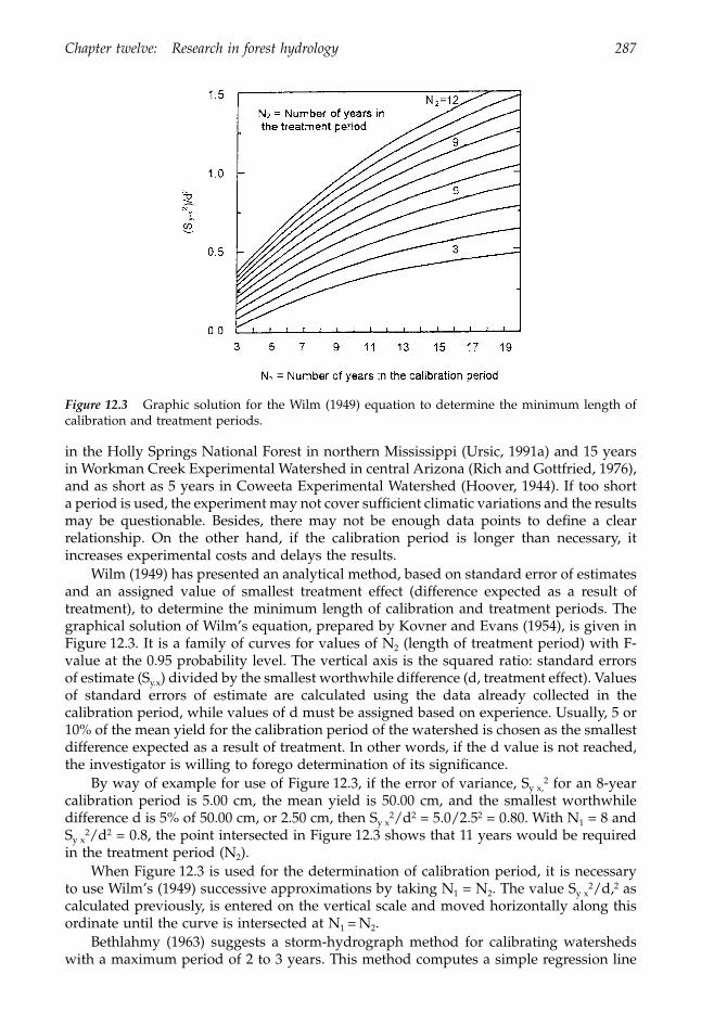
Chapter twelve: Research in forest hydrology 287
in the Holly Springs National Forest in northern Mississippi (Ursic, 1991a) and 15 yearsin Workman Creek Experimental Watershed in central Arizona (Rich and Gottfried, 1976),and as short as 5 years in Coweeta Experimental Watershed (Hoover, 1944). If too shorta period is used, the experiment may not cover sufficient climatic variations and the resultsmay be questionable. Besides, there may not be enough data points to define a clearrelationship. On the other hand, if the calibration period is longer than necessary, itincreases experimental costs and delays the results.
Wilm (1949) has presented an analytical method, based on standard error of estimatesand an assigned value of smallest treatment effect (difference expected as a result oftreatment), to determine the minimum length of calibration and treatment periods. Thegraphical solution of Wilm’s equation, prepared by Kovner and Evans (1954), is given inFigure 12.3. It is a family of curves for values of N
2
(length of treatment period) with F-value at the 0.95 probability level. The vertical axis is the squared ratio: standard errorsof estimate (S
y.x
) divided by the smallest worthwhile difference (d, treatment effect). Valuesof standard errors of estimate are calculated using the data already collected in thecalibration period, while values of d must be assigned based on experience. Usually, 5 or10% of the mean yield for the calibration period of the watershed is chosen as the smallestdifference expected as a result of treatment. In other words, if the d value is not reached,the investigator is willing to forego determination of its significance.
By way of example for use of Figure 12.3, if the error of variance, S
y x,2
for an 8-yearcalibration period is 5.00 cm, the mean yield is 50.00 cm, and the smallest worthwhiledifference d is 5% of 50.00 cm, or 2.50 cm, then S
y x2
/d
2
= 5.0/2.5
2
= 0.80. With N
1
= 8 andS
y x2
/d
2
= 0.8, the point intersected in Figure 12.3 shows that 11 years would be requiredin the treatment period (N
2
).When Figure 12.3 is used for the determination of calibration period, it is necessary
to use Wilm’s (1949) successive approximations by taking N
1
= N
2
. The value S
y x2
/d,
2
ascalculated previously, is entered on the vertical scale and moved horizontally along thisordinate until the curve is intersected at N
1
=
N
2
.Bethlahmy (1963) suggests a storm-hydrograph method for calibrating watersheds
with a maximum period of 2 to 3 years. This method computes a simple regression line
Figure 12.3
Graphic solution for the Wilm (1949) equation to determine the minimum length ofcalibration and treatment periods.
1363_C12_fm Page 287 Wednesday, December 4, 2002 7:45 AM
288 Forest Hydrology: An Introduction to Water and Forests
on maximum stage rise and time to peak obtained from storm hydrographs between thetwo watersheds for the pretreatment year and a regression line for the posttreatment years.Pretreatment and posttreatment regression lines are then compared for statistical signifi-cance of the treatment. In this method, only storms that cover both watersheds may beused in the analysis.
Calibration and analysis based on individual runoff events is particularly useful inwatersheds where changes in overland flow are of primary concern. Ursic and Popham(1967) showed that the accumulation of 30 consecutive runoff events is sufficient to definea reliable relationship. In the southern Coastal Plain, storms occurring in a given year maynot be fully representative, but 2 or 3 years should be sufficient.
e. Treatment effects.
The differences in streamflow between the observed and thepredicted (for the conditions as if the watershed had not been treated) values calculatedby calibration equations such as Equation 12.1 are the treatment effects,
D
q = y
-
y
x
. Todetermine statistical significance of the treatment effects, a posttreatment regression onstreamflow between the control and treated watersheds can be developed. The posttreat-ment regression is then compared to the pretreatment (calibration) regression on theirslopes and adjusted means (elevations) by covariance analysis for statistical significanceat a preselected alpha level (Li, 1964; Troendle and King, 1985; Bent, 1994). A numericalexample for the statistical tests is given in part IV. It is advisable, however, that the periodsbefore and after treatment be as close to the same length as possible so that they have anequal opportunity to be exposed to variations in climate and other environmental factors(Wilm, 1949). Also, a difference between the observed and estimated streamflow can beconsidered statistically significant if the deviation exceeds a preselected (usually 95%)confidence interval about the regression line (Harr et al., 1979; Hornbeck et al., 1987).
As was explained earlier, deforestation is generally expected to cause an increase instreamflow. The magnitudes of increase, although highly variable, seem to be positivelyaffected by annual precipitation and are gradually reduced to levels at the pretreatmentperiod due to regrowth of vegetation (Bosch and Hewlett, 1982; Troendle and King, 1985).Thus, a two-step analysis was used to study the effect of forest understory cutting andregrowth on streamflow at Coweeta Hydrologic Laboratory, North Carolina (Johnson andKovner, 1954). First, the increase in annual streamflow was estimated using a simple linear-regression model similar to Equation 12.1 developed for the calibration period. Then theestimated treatment effect in annual water yield (
D
q) was regressed with annual precipi-tation (P) and a time factor in the following fashion:
D
q
(T)
= a + b
1
(P) + b
2
(T) (12.5)
where T is the time since treatment in years; P is annual precipitation; and a, b
1
, and b
2
are regression coefficients. The time factor (T) and streamflow from the control watershed(x) were also used together in the following multiregression model to evaluate treatmenteffects (Schneider and Ayer, 1961; Baker, 1986):
D
q
(T)
= a + b
1
(x) + b
2
(T)(x) (12.6)
The technique of double-mass analysis (Merriam, 1937; Chang and Lee, 1974) has alsobeen applied to evaluate the significance of treatment effects (Anderson, 1955; Chang andCrowley, 1997). This method plots the accumulated annual streamflow of the controlwatershed against the accumulated annual streamflow of the treatment watershed. Theplot appears as a straight line with minor variations if there was no treatment effect or
1363_C12_fm Page 288 Wednesday, December 4, 2002 7:45 AM
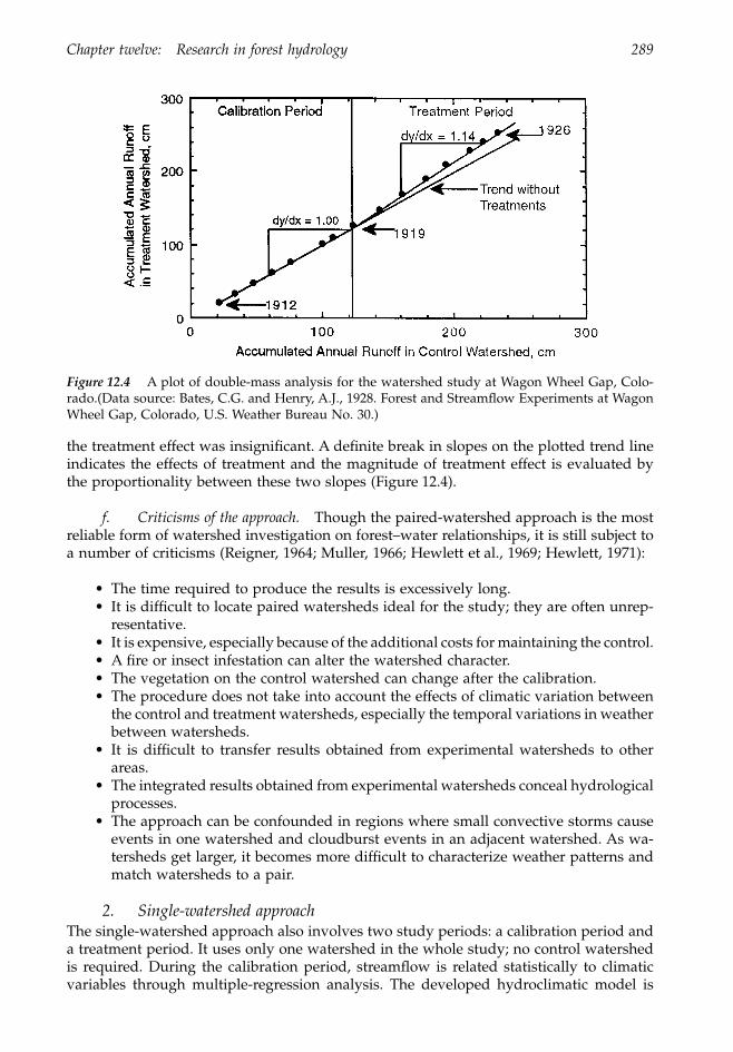
Chapter twelve: Research in forest hydrology 289
the treatment effect was insignificant. A definite break in slopes on the plotted trend lineindicates the effects of treatment and the magnitude of treatment effect is evaluated bythe proportionality between these two slopes (Figure 12.4).
f. Criticisms of the approach.
Though the paired-watershed approach is the mostreliable form of watershed investigation on forest–water relationships, it is still subject toa number of criticisms (Reigner, 1964; Muller, 1966; Hewlett et al., 1969; Hewlett, 1971):
• The time required to produce the results is excessively long.• It is difficult to locate paired watersheds ideal for the study; they are often unrep-
resentative.• It is expensive, especially because of the additional costs for maintaining the control.• A fire or insect infestation can alter the watershed character.• The vegetation on the control watershed can change after the calibration.• The procedure does not take into account the effects of climatic variation between
the control and treatment watersheds, especially the temporal variations in weatherbetween watersheds.
• It is difficult to transfer results obtained from experimental watersheds to otherareas.
• The integrated results obtained from experimental watersheds conceal hydrologicalprocesses.
• The approach can be confounded in regions where small convective storms causeevents in one watershed and cloudburst events in an adjacent watershed. As wa-tersheds get larger, it becomes more difficult to characterize weather patterns andmatch watersheds to a pair.
2. Single-watershed approach
The single-watershed approach also involves two study periods: a calibration period anda treatment period. It uses only one watershed in the whole study; no control watershedis required. During the calibration period, streamflow is related statistically to climaticvariables through multiple-regression analysis. The developed hydroclimatic model is
Figure 12.4
A plot of double-mass analysis for the watershed study at Wagon Wheel Gap, Colo-rado.(Data source: Bates, C.G. and Henry, A.J., 1928. Forest and Streamflow Experiments at WagonWheel Gap, Colorado, U.S. Weather Bureau No. 30.)
1363_C12_fm Page 289 Wednesday, December 4, 2002 7:45 AM
290 Forest Hydrology: An Introduction to Water and Forests
then used to estimate streamflow for the treatment period. The treatment effects onstreamflow are calculated by the differences between observed and estimated values.
By way of example, the following equation was developed to estimate streamflow forthe 1964–1972 period of the forested La Nana Creek watershed in east Texas (Chang andSayok, 1990):
Q = –396.16 + 194.23(P)/(T
2
) (12.7)
where Q and P were annual streamflow and precipitation, respectively, in mm, and T wasannual air temperature in
∞
C. Equation 12.7 was then employed to estimate streamflowfor the 1973–1984 period, in which the lower portion of the watershed went through arapid and intensive urbanization. Comparing the observed streamflow to that estimatedby Equation 12.7, urbanization in the lower section of the 80 km
2
watershed increasedstreamflow by 85.2 mm year
-1
.The treatment effect can also be evaluated by plotting the accumulated values of
precipitation against accumulated runoff in a double-mass analysis (Potts, 1984). A breakin slopes on the double-mass curve indicates the effect of land-use treatments and iscalculated by the difference in slopes between these two periods (Bernt and Swank, 1970;Betson, 1979; Potts, 1984). However, the use of double-mass curves is rather crude andprovides no measure of random error (Reigner, 1964). In northern California, Pitt et al.(1978) used runoff/precipitation ratio as a criterion to evaluate the effects of convertingwoody vegetation into brush and weather patterns on streamflow among three studyperiods on a single watershed. They found that grassy watershed released 39% more totalrunoff than did woody vegetation.
Thornthwaite’s water-balance model has also been employed to evaluate treatmenteffects in four single watersheds in New York (Muller, 1966). The model is based on theconcept of potential evapotranspiration (PE) computed by mean air temperature and bya temperature-based heat index. By using monthly PE and actual evapotranspiration andprecipitation, the monthly distribution of water deficit, soil water utilization, soil moisturerecharge, and surplus water can be characterized for the area (Thornthwaite and Mather,1955; Thornthwaite and Mather, 1957). The method takes into account much of the monthlyand seasonal variation of the hydroclimatological elements in the analysis. However, theevaporation equation used in this method fails to explain the difference in the plant coveron the watersheds (Hewlett et al., 1969).
The single-watershed approach requires a calibration period longer than the paired-watershed approach, and hence is subject to additional costs and greater environmentalrisks. This may be due to two reasons. First, it is more difficult to estimate streamflowfrom climatic variables than from streamflow of a nearby watershed because of datavariability. Second, because of budget constraints and the consideration of site accessibility,the climatic data used in the watershed study are usually collected from a single site nearthe stream-gaging station or even out of the watershed. In this case, the climatic data aremost likely not representative of the climatic conditions of the entire watershed.
In the paired-watershed approach, if forests in one watershed are destroyed due tonatural or man-made disasters, study of the other watershed can proceed using the single-watershed approach.
3. Replicated-watershed approach
The results obtained from the paired- and single-watershed approaches refer to the specificsite conditions. Measurements made at a single site may not be representative of the entirearea, and its experimental errors are difficult to assess. This leads to the use of the
1363_C12_fm Page 290 Wednesday, December 4, 2002 7:45 AM
Chapter twelve: Research in forest hydrology 291
replicated-watershed approach (Blackburn et al., 1986; Ursic, 1991b). Replication, random-ization, and control are the three basic principles of experimental design. However, thisapproach is not common in watershed studies partly due to the variation of watershedenvironmental conditions. Ideal watersheds for replication are very difficult to find. Rep-lication is general practice in small-plot studies (Shahlaee et al., 1991).
Careful design of a replicated watershed study does not preclude a calibration periodas was discussed in the paired-watershed approaches. Replication allows researchers toevaluate whether the treatments have caused a significant effect or not. It does not revealthe magnitude of the treatment effects. Without such information, watershed-modelingstudies cannot be validated.
B. Upstream–downstream approach
The upstream–downstream approach is often used in studying water quality, habitatquality, and aquatic organisms as affected by existing land-use conditions, land treatments,or natural disasters. It selects two sampling sites along a reach for study, one above andone below the project area. The upstream site is a control for the detection of changes dueto downstream treatments. Differences in concentrations or other quality parametersbetween downstream and upstream are attributable to the conditions of the project (treat-ment) area. Key elements of this approach are the similarity and simultaneous monitoringof the two sampling sites. They should be located as close to the project area as practicableso that the confounding differences between the two sites can be minimized (MacDonaldet al., 1991). However, the upstream control site should be far enough from the down-stream treatment effect. The method generally does not use a calibration period; measure-ments from an untreated reach are adequate for comparisons if the site is properly located(Gluns and Toews, 1989; EPA, 1997). The approach is often criticized for streamflowautocorrelation between the upstream and downstream sites. If practicable, three to fourreplicates should be established in the same area for statistical inference.
C. Experimental plots
Experimental plots are blocks of undisturbed soil surrounded by bricks, concrete blocks,or even plywood installed in the field. The lower end of each plot is equipped withinstruments or containers to monitor surface and subsurface runoff and to catch sedimentunder various forest conditions (Figure 12.5). Since these plot watersheds are relativelysmall — 0.01 to 0.1 ha in size — it is possible to install them on relatively homogeneousconditions with sufficient replicas with respect to soils, topography, vegetation, and cli-matic conditions. Such homogeneous plots, with sufficient replicas, allow the effects ofvegetation manipulation on runoff to be monitored directly from these plot watershedswithout need for a calibration period. Compared to the paired- and single-watershedapproaches, the costs and time required in plot studies are largely reduced.
Lysimeters are another version of the plot-study approach. A lysimeter is a wholeblock of soil (bottom and sides) completely sealed from its surroundings. Usually a scale-balance and drainage pipes are installed below the block; evapotranspiration (ET) of theblock can then be calculated by the loss in weight, and soil water percolation can becompletely collected, between two consecutive periods. A design like this is referred toas a weighing lysimeter (Harrold and Dreibelbis, 1958; Kirkham et al., 1984). Sometimesthe whole soil block is in an inner tank that floats on an outer tank filled with liquid andinstalled in the soil. ET of the soil tank is evaluated by the fluctuation of water level inthe water tank through Archimedes’ principle. This type of tank is called a floatinglysimeter (Chang et al., 1997). Since the hydrologic components can be measured andcalculated precisely, lysimeters are a common tool in ET and soil-percolation studies. It is
1363_C12_fm Page 291 Wednesday, December 4, 2002 7:45 AM
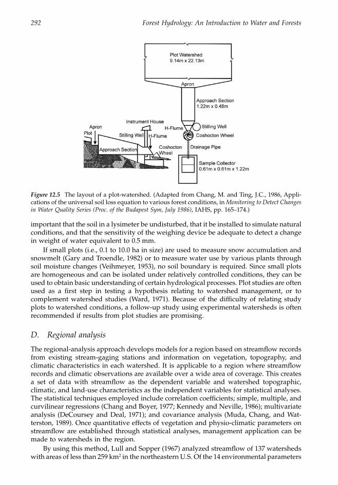
292 Forest Hydrology: An Introduction to Water and Forests
important that the soil in a lysimeter be undisturbed, that it be installed to simulate naturalconditions, and that the sensitivity of the weighing device be adequate to detect a changein weight of water equivalent to 0.5 mm.
If small plots (i.e., 0.1 to 10.0 ha in size) are used to measure snow accumulation andsnowmelt (Gary and Troendle, 1982) or to measure water use by various plants throughsoil moisture changes (Veihmeyer, 1953), no soil boundary is required. Since small plotsare homogeneous and can be isolated under relatively controlled conditions, they can beused to obtain basic understanding of certain hydrological processes. Plot studies are oftenused as a first step in testing a hypothesis relating to watershed management, or tocomplement watershed studies (Ward, 1971). Because of the difficulty of relating studyplots to watershed conditions, a follow-up study using experimental watersheds is oftenrecommended if results from plot studies are promising.
D. Regional analysis
The regional-analysis approach develops models for a region based on streamflow recordsfrom existing stream-gaging stations and information on vegetation, topography, andclimatic characteristics in each watershed. It is applicable to a region where streamflowrecords and climatic observations are available over a wide area of coverage. This createsa set of data with streamflow as the dependent variable and watershed topographic,climatic, and land-use characteristics as the independent variables for statistical analyses.The statistical techniques employed include correlation coefficients; simple, multiple, andcurvilinear regressions (Chang and Boyer, 1977; Kennedy and Neville, 1986); multivariateanalysis (DeCoursey and Deal, 1971); and covariance analysis (Muda, Chang, and Wat-terston, 1989). Once quantitative effects of vegetation and physio-climatic parameters onstreamflow are established through statistical analyses, management application can bemade to watersheds in the region.
By using this method, Lull and Sopper (1967) analyzed streamflow of 137 watershedswith areas of less than 259 km
2
in the northeastern U.S. Of the 14 environmental parameters
Figure 12.5
The layout of a plot-watershed. (Adapted from Chang, M. and Ting, J.C., 1986, Appli-cations of the universal soil loss equation to various forest conditions, in
Monitoring to Detect Changesin Water Quality Series (Proc. of the Budapest Sym, July 1986)
, IAHS, pp. 165–174.)
1363_C12_fm Page 292 Wednesday, December 4, 2002 7:45 AM
Chapter twelve: Research in forest hydrology 293
analyzed, annual streamflow was found to be positively affected by annual precipitation,percent of forest cover, and elevation, and was negatively affected by mean maximumtemperature for July. About 61% of annual streamflows were accounted for by the fourparameters. The positive effect of percent forest area on annual streamflow, which seemsto be contradictory to the central concept discussed earlier, is due to the forest environmentof the region. In the Northeast, forest cover generally increases with elevation, which inturn is associated with greater precipitation, steeper slopes, shallower soils, cooler tem-peratures, and lower evapotranspiration. These environmental factors may result ingreater streamflow.
In forested east Texas, Chang and Waters (1984) developed the following equationwith a standard error of estimate 11.8% of the observed mean to estimate annual stream-flow for 19 unregulated, natural streams:
Q = –2018 + 4.16(P
s
) + 50.91(T) – 1.98(FO) (12.8)
where Q and P
s
are annual streamflow and spring precipitation (March + April + May),respectively, in mm, T is annual air temperature in
∞
C, and FO is percent forest area. Theresults show that a reduction of watershed forested area by 20%, other things being equal,would increase water yield about 40 mm/year
-1
, and the difference in annual streamflowbetween full forest cover and bare watersheds could be as much as 200 mm. This differencewas much less than that reported in western Oregon (Harr, 1983) and Coweeta, NorthCarolina (Hewlett and Hibbert, 1961), about the same as that in West Virginia (Kochender-fer and Aubertin, 1975), and greater than that in Arizona and New Mexico (Hibbert, 1981).Clearcutting followed by site preparations is a common practice for forest regenerationin east Texas. The effect of forest clearcutting on the first year streamflow could beevaluated by Equation 12.8.
E. Watershed simulation
Experimental watershed studies are costly, time consuming, weather dependent, anddifficult to replicate. Hydrologic simulation provides an alternative approach for rapidlyassessing forest practices and other land management. It is a means of predicting water-shed response to various weather conditions and management strategies. The simulationcan be for estimating streamflow, sediment, and water quality. The time frame of theestimates can be for (1) single rainfall-runoff event and routing programs, (2) continuoussimulation programs, or (3) long-term averages.
First, a conceptual hydrologic-balance model needs to be used. Then various physio-climatic models are developed to estimate components of the conceptual model in thehydrologic processes. The input component of precipitation can be based first on obser-vations for calibration and verification of the developed model and later based on prede-termined scenarios for management purposes. The effects of forest cover and other man-agement activities on streamflow can then be simulated by computing these variouscomponent models and summing all components to solve the conceptual model. It isimportant that physical laws governing runoff processes are fully understood beforereliable data can be simulated.
By way of example, Figure 12.6 is the conceptualization of a watershed monthlyhydrologic model developed by Allred and Haan (1996). The model, “SWMHMS — smallwatershed monthly hydrologic modeling system,” simulates monthly runoff from a smallnonurban watershed. The rainfall input in the model is partitioned into three components:(1) surface and vegetation interception loss, (2) soil infiltration and soil-water reservoir,and (3) surface runoff. Soil water is first subject to ET loss and then to soil percolation asinterflow and groundwater if the excess soil water is above field capacity. Base flow from
1363_C12_fm Page 293 Wednesday, December 4, 2002 7:45 AM
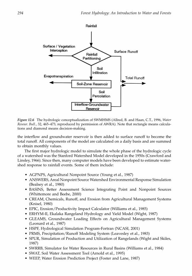
294 Forest Hydrology: An Introduction to Water and Forests
the interflow and groundwater reservoir is then added to surface runoff to become thetotal runoff. All components of the model are calculated on a daily basis and are summedto obtain monthly values.
The first major hydrologic model to simulate the whole phase of the hydrologic cycleof a watershed was the Stanford Watershed Model developed in the 1950s (Crawford andLinsley, 1966). Since then, many computer models have been developed to estimate water-shed response to rainfall events. Some of them include:
• AGPNPS, Agricultural Nonpoint Source (Young et al., 1987)• ANSWERS, Areal Nonpoint Source Watershed Environmental Response Simulation
(Bealsey et al., 1980)• BASINS, Better Assessment Science Integrating Point and Nonpoint Sources
(Whittemore and Beebe, 2000)• CREAM, Chemicals, Runoff, and Erosion from Agricultural Management Systems
(Knisel, 1980)• EPIC, Erosion/Productivity Impact Calculator (Williams et al., 1985)• ERHYM-II, Ekalaka Rangeland Hydrology and Yield Model (Wight, 1987)• GLEAMS, Groundwater Loading Effects on Agricultural Management Systems
(Leonard et al., 1987)• HSPF, Hydrological Simulation Program-Fortran (NCASI, 2001)• PRMS, Precipitation/Runoff Modeling System (Leavesley et al., 1983)• SPUR, Simulation of Production and Utilization of Rangelands (Wight and Skiles,
1987)• SWRRB, Simulator for Water Resources in Rural Basins (Williams et al., 1984)• SWAT, Soil Water Assessment Tool (Arnold et al., 1995)• WEEP, Water Erosion Prediction Project (Foster and Lane, 1987)
Figure 12.6
The hydrologic conceptualization of SWMHMS (Allred, B. and Haan, C.T., 1996,
WaterResour. Bull.
, 32, 465–473, reproduced by permission of AWRA). Note that rectangle means calcula-tions and diamond means decision-making.
1363_C12_fm Page 294 Wednesday, December 4, 2002 7:45 AM
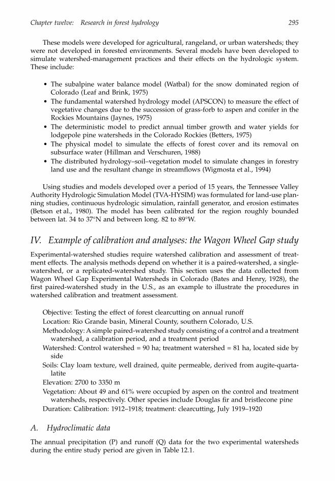
Chapter twelve: Research in forest hydrology 295
These models were developed for agricultural, rangeland, or urban watersheds; theywere not developed in forested environments. Several models have been developed tosimulate watershed-management practices and their effects on the hydrologic system.These include:
• The subalpine water balance model (Watbal) for the snow dominated region ofColorado (Leaf and Brink, 1975)
• The fundamental watershed hydrology model (APSCON) to measure the effect ofvegetative changes due to the succession of grass-forb to aspen and conifer in theRockies Mountains (Jaynes, 1975)
• The deterministic model to predict annual timber growth and water yields forlodgepole pine watersheds in the Colorado Rockies (Betters, 1975)
• The physical model to simulate the effects of forest cover and its removal onsubsurface water (Hillman and Verschuren, 1988)
• The distributed hydrology–soil–vegetation model to simulate changes in forestryland use and the resultant change in streamflows (Wigmosta et al., 1994)
Using studies and models developed over a period of 15 years, the Tennessee ValleyAuthority Hydrologic Simulation Model (TVA-HYSIM) was formulated for land-use plan-ning studies, continuous hydrologic simulation, rainfall generator, and erosion estimates(Betson et al., 1980). The model has been calibrated for the region roughly boundedbetween lat. 34 to 37°N and between long. 82 to 89°W.
IV. Example of calibration and analyses: the Wagon Wheel Gap study
Experimental-watershed studies require watershed calibration and assessment of treat-ment effects. The analysis methods depend on whether it is a paired-watershed, a single-watershed, or a replicated-watershed study. This section uses the data collected fromWagon Wheel Gap Experimental Watersheds in Colorado (Bates and Henry, 1928), thefirst paired-watershed study in the U.S., as an example to illustrate the procedures inwatershed calibration and treatment assessment.
Objective: Testing the effect of forest clearcutting on annual runoffLocation: Rio Grande basin, Mineral County, southern Colorado, U.S.Methodology: A simple paired-watershed study consisting of a control and a treatment
watershed, a calibration period, and a treatment periodWatershed: Control watershed = 90 ha; treatment watershed = 81 ha, located side by
sideSoils: Clay loam texture, well drained, quite permeable, derived from augite-quarta-
latiteElevation: 2700 to 3350 mVegetation: About 49 and 61% were occupied by aspen on the control and treatment
watersheds, respectively. Other species include Douglas fir and bristlecone pineDuration: Calibration: 1912–1918; treatment: clearcutting, July 1919–1920
A. Hydroclimatic data
The annual precipitation (P) and runoff (Q) data for the two experimental watershedsduring the entire study period are given in Table 12.1.
1363_C12_fm Page 295 Wednesday, December 4, 2002 7:45 AM
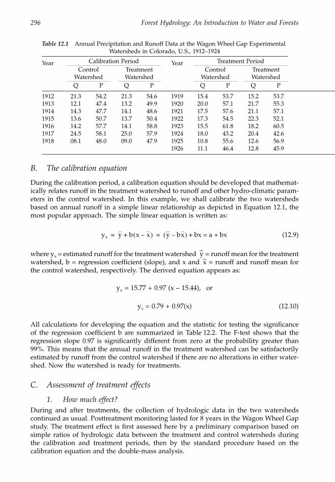
296 Forest Hydrology: An Introduction to Water and Forests
B. The calibration equation
During the calibration period, a calibration equation should be developed that mathemat-ically relates runoff in the treatment watershed to runoff and other hydro-climatic param-eters in the control watershed. In this example, we shall calibrate the two watershedsbased on annual runoff in a simple linear relationship as depicted in Equation 12.1, themost popular approach. The simple linear equation is written as:
(12.9)
where y
x
= estimated runoff for the treatment watershed –y = runoff mean for the treatmentwatershed, b = regression coefficient (slope), and x and –x = runoff and runoff mean forthe control watershed, respectively. The derived equation appears as:
y
x
= 15.77 + 0.97 (x – 15.44), or
y
x
= 0.79 + 0.97(x) (12.10)
All calculations for developing the equation and the statistic for testing the significanceof the regression coefficient b are summarized in Table 12.2. The F-test shows that theregression slope 0.97 is significantly different from zero at the probability greater than99%. This means that the annual runoff in the treatment watershed can be satisfactorilyestimated by runoff from the control watershed if there are no alterations in either water-shed. Now the watershed is ready for treatments.
C. Assessment of treatment effects
1. How much effect?
During and after treatments, the collection of hydrologic data in the two watershedscontinued as usual. Posttreatment monitoring lasted for 8 years in the Wagon Wheel Gapstudy. The treatment effect is first assessed here by a preliminary comparison based onsimple ratios of hydrologic data between the treatment and control watersheds duringthe calibration and treatment periods, then by the standard procedure based on thecalibration equation and the double-mass analysis.
Table 12.1
Annual Precipitation and Runoff Data at the Wagon Wheel Gap Experimental
Watersheds in Colorado, U.S., 1912–1924
Year
Calibration Period Year
Treatment PeriodControl
WatershedTreatment
WatershedControl
WatershedTreatment
WatershedQ P Q P Q P Q P
1912 21.3 54.2 21.3 54.6 1919 15.4 53.7 15.2 53.71913 12.1 47.4 13.2 49.9 1920 20.0 57.1 21.7 55.31914 14.3 47.7 14.1 48.6 1921 17.5 57.6 21.1 57.11915 13.6 50.7 13.7 50.4 1922 17.3 54.5 22.3 52.11916 14.2 57.7 14.1 58.8 1923 15.5 61.8 18.2 60.51917 24.5 58.1 25.0 57.9 1924 18.0 43.2 20.4 42.61918 08.1 48.0 09.0 47.9 1925 10.8 55.6 12.6 56.9
1926 11.1 46.4 12.8 45.9
yx y b x – x( )+ y bx–( ) bx = a + bx+= =
1363_C12_fm Page 296 Wednesday, December 4, 2002 7:45 AM
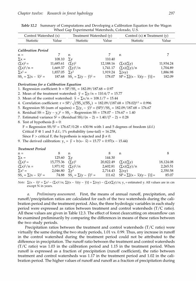
Chapter twelve: Research in forest hydrology 297
a. Preliminary assessment. First, the means of annual runoff, precipitation, andrunoff/precipitation ratios are calculated for each of the two watersheds during the cali-bration period and the treatment period. Also, the three hydrologic variables in each studyperiod were expressed as ratios between treatment and control watersheds (T/C ratio).All these values are given in Table 12.3. The effect of forest clearcutting on streamflow canbe examined preliminarily by comparing the differences in means of these ratios betweenthe two study periods.
Precipitation ratios between the treatment and control watersheds (T/C ratio) werevirtually the same during the two study periods, 1.01 vs. 0.99. Thus, any increase in runoffin the control watershed during the treatment period could not be attributed to thedifference in precipitation. The runoff ratio between the treatment and control watersheds(T/C ratio) was 1.03 in the calibration period and 1.15 in the treatment period. Whenrunoff is expressed as a fraction of precipitation (runoff coefficient), the ratio betweentreatment and control watersheds was 1.17 in the treatment period and 1.02 in the cali-bration period. The higher values of runoff and runoff as a fraction of precipitation during
Table 12.2 Summary of Computations and Developing a Calibration Equation for the Wagon Wheel Gap Experimental Watersheds, Colorado, U.S.
Control Watershed (x) Treatment Watershed (y) Control (x) ¥¥¥¥ Treatment (y)Statistic Value Statistic Value Statistic Value
Calibration Periodn = 7 n 7 n 7Âx = 108.10 Ây 110.40(Âx)2 = 11,685.61 (Ây)2 12,188.16 (Âx)(Ây) 11,934.24(Âx)2/n = 1,669.37 (Ây)2/n 1,741.17 (Âx)(Ây)/n 1,704.89Âx2 = 1,857.05 Ây2 1,919.24 Â(xy) 1,886.98SSx = Â(x – –x)2 = 187.68 SSy = Â(y – –y)2 = 178.07 SP = Â[(x – –x)(y – –y)] = 182.09
Derivations for a Calibration Equation1. Regression coefficient: b = SP/SSx = 182.09/187.68 = 0.972. Mean of the treatment watershed: –y = Ây/n = 110.4/7 = 15.773. Mean of the control watershed: –x = Âx/n = 108.1/7 = 15.444. Correlation coefficient: r = SP/ = 182.09/(187.68 ¥ 178.02)0.5 = 0.9965. Regression SS (sum of squires) = Â(yx –
–y)2 = (SP)2/SSx = 182.09/187.68 = 176.676. Residual SS = Â(y - yx)2 = SSy - Regression SS = 178.07 - 176.67 = 1.407. Estimated variance S2 = (Residual SS)/(n - 2) = 1.40/(7 - 2) = 0.288. Test of hypothesis b = 0:
F = Regression SS/S2 = 176.67/0.28 = 630.96 with 1 and 5 degrees of freedom (d.f.)Critical F @ 1 and 5 d.f.; 1% probability (one-tail) = 16.258,Since F > critical F, the hypothesis is rejected and b π 0.
9. The derived calibration: yx =–y + b(x– –x) = 15.77 + 0.97(x - 15.44)
Treatment Periodn = 8 n 8 n 8Âx = 125.60 Ây 144.30(Âx)2 = 15,775.36 (Ây)2 20,822.49 (Âx)(Ây) 18,124.08(Âx)2/n = 1,971.92 (Ây)2/n 2,602.81 (Âx)(Ây)/n 2,265.51Âx2 = 2,046.80 Ây2 2,714.43 Â(xy) 2,350.58SSx = Â(x – –x)2 = 74.88 SSy = Â(y – –y)2 = 111.62 SP = Â[(x – –x)(y – –y)] = 85.07
Note: Â(x – –x)2 = Âx2 - (Âx)2/n; Â[(x – –x)(y – –y)] = Â(xy) - (Âx)(Ây)/n; yx = estimated y. All values are in cmexcept N in years.
SSx( ) SSy( )
1363_C12_fm Page 297 Wednesday, December 4, 2002 7:45 AM
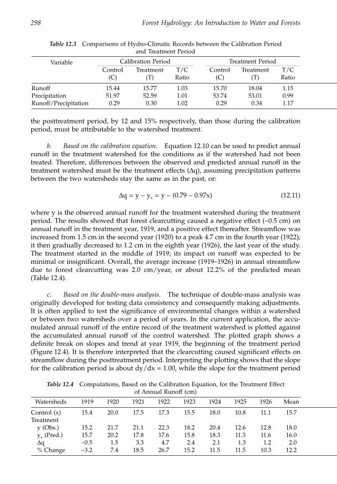
298 Forest Hydrology: An Introduction to Water and Forests
the posttreatment period, by 12 and 15% respectively, than those during the calibrationperiod, must be attributable to the watershed treatment.
b. Based on the calibration equation. Equation 12.10 can be used to predict annualrunoff in the treatment watershed for the conditions as if the watershed had not beentreated. Therefore, differences between the observed and predicted annual runoff in thetreatment watershed must be the treatment effects (Dq), assuming precipitation patternsbetween the two watersheds stay the same as in the past, or:
Dq = y – yx = y – (0.79 – 0.97x) (12.11)
where y is the observed annual runoff for the treatment watershed during the treatmentperiod. The results showed that forest clearcutting caused a negative effect (-0.5 cm) onannual runoff in the treatment year, 1919, and a positive effect thereafter. Streamflow wasincreased from 1.5 cm in the second year (1920) to a peak 4.7 cm in the fourth year (1922);it then gradually decreased to 1.2 cm in the eighth year (1926), the last year of the study.The treatment started in the middle of 1919; its impact on runoff was expected to beminimal or insignificant. Overall, the average increase (1919–1926) in annual streamflowdue to forest clearcutting was 2.0 cm/year, or about 12.2% of the predicted mean(Table 12.4).
c. Based on the double-mass analysis. The technique of double-mass analysis wasoriginally developed for testing data consistency and consequently making adjustments.It is often applied to test the significance of environmental changes within a watershedor between two watersheds over a period of years. In the current application, the accu-mulated annual runoff of the entire record of the treatment watershed is plotted againstthe accumulated annual runoff of the control watershed. The plotted graph shows adefinite break on slopes and trend at year 1919, the beginning of the treatment period(Figure 12.4). It is therefore interpreted that the clearcutting caused significant effects onstreamflow during the posttreatment period. Interpreting the plotting shows that the slopefor the calibration period is about dy/dx = 1.00, while the slope for the treatment period
Table 12.3 Comparisons of Hydro-Climatic Records between the Calibration Period and Treatment Period
Variable Calibration Period Treatment PeriodControl
(C)Treatment
(T)T/C Ratio
Control (C)
Treatment (T)
T/C Ratio
Runoff 15.44 15.77 1.03 15.70 18.04 1.15Precipitation 51.97 52.59 1.01 53.74 53.01 0.99Runoff/Precipitation 0.29 0.30 1.02 0.29 0.34 1.17
Table 12.4 Computations, Based on the Calibration Equation, for the Treatment Effect of Annual Runoff (cm)
Watersheds 1919 1920 1921 1922 1923 1924 1925 1926 Mean
Control (x) 15.4 20.0 17.5 17.3 15.5 18.0 10.8 11.1 15.7Treatment
y (Obs.) 15.2 21.7 21.1 22.3 18.2 20.4 12.6 12.8 18.0yx (Pred.) 15.7 20.2 17.8 17.6 15.8 18.3 11.3 11.6 16.0Dq -0.5 1.5 3.3 4.7 2.4 2.1 1.3 1.2 2.0% Change -3.2 7.4 18.5 26.7 15.2 11.5 11.5 10.3 12.2
1363_C12_fm Page 298 Wednesday, December 4, 2002 7:45 AM
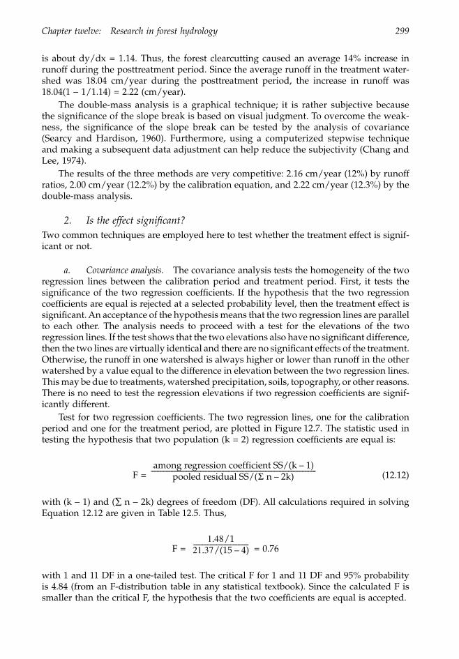
Chapter twelve: Research in forest hydrology 299
is about dy/dx = 1.14. Thus, the forest clearcutting caused an average 14% increase inrunoff during the posttreatment period. Since the average runoff in the treatment water-shed was 18.04 cm/year during the posttreatment period, the increase in runoff was18.04(1 - 1/1.14) = 2.22 (cm/year).
The double-mass analysis is a graphical technique; it is rather subjective becausethe significance of the slope break is based on visual judgment. To overcome the weak-ness, the significance of the slope break can be tested by the analysis of covariance(Searcy and Hardison, 1960). Furthermore, using a computerized stepwise techniqueand making a subsequent data adjustment can help reduce the subjectivity (Chang andLee, 1974).
The results of the three methods are very competitive: 2.16 cm/year (12%) by runoffratios, 2.00 cm/year (12.2%) by the calibration equation, and 2.22 cm/year (12.3%) by thedouble-mass analysis.
2. Is the effect significant?Two common techniques are employed here to test whether the treatment effect is signif-icant or not.
a. Covariance analysis. The covariance analysis tests the homogeneity of the tworegression lines between the calibration period and treatment period. First, it tests thesignificance of the two regression coefficients. If the hypothesis that the two regressioncoefficients are equal is rejected at a selected probability level, then the treatment effect issignificant. An acceptance of the hypothesis means that the two regression lines are parallelto each other. The analysis needs to proceed with a test for the elevations of the tworegression lines. If the test shows that the two elevations also have no significant difference,then the two lines are virtually identical and there are no significant effects of the treatment.Otherwise, the runoff in one watershed is always higher or lower than runoff in the otherwatershed by a value equal to the difference in elevation between the two regression lines.This may be due to treatments, watershed precipitation, soils, topography, or other reasons.There is no need to test the regression elevations if two regression coefficients are signif-icantly different.
Test for two regression coefficients. The two regression lines, one for the calibrationperiod and one for the treatment period, are plotted in Figure 12.7. The statistic used intesting the hypothesis that two population (k = 2) regression coefficients are equal is:
F = (12.12)
with (k - 1) and (Â n - 2k) degrees of freedom (DF). All calculations required in solvingEquation 12.12 are given in Table 12.5. Thus,
F = = 0.76
with 1 and 11 DF in a one-tailed test. The critical F for 1 and 11 DF and 95% probabilityis 4.84 (from an F-distribution table in any statistical textbook). Since the calculated F issmaller than the critical F, the hypothesis that the two coefficients are equal is accepted.
among regression coefficient SS/(k – 1) pooled residual SS/(S n – 2k)
-----------------------------------------------------------------------------------------------------------
1.48/121.37/(15 – 4)------------------------------------
1363_C12_fm Page 299 Wednesday, December 4, 2002 7:45 AM
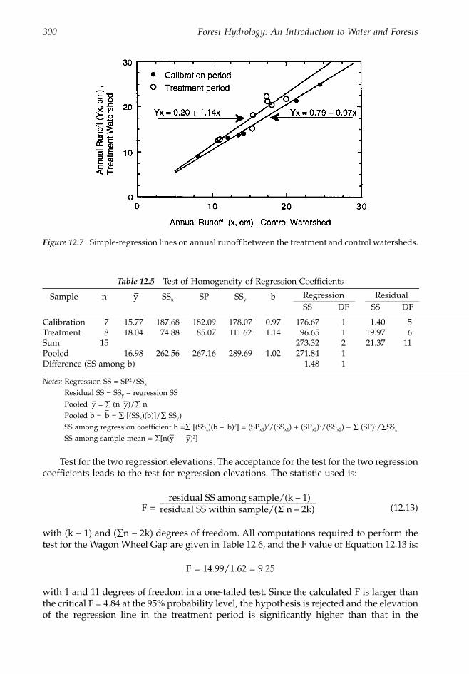
300 Forest Hydrology: An Introduction to Water and Forests
Test for the two regression elevations. The acceptance for the test for the two regressioncoefficients leads to the test for regression elevations. The statistic used is:
F = (12.13)
with (k - 1) and (Ân - 2k) degrees of freedom. All computations required to perform thetest for the Wagon Wheel Gap are given in Table 12.6, and the F value of Equation 12.13 is:
F = 14.99/1.62 = 9.25
with 1 and 11 degrees of freedom in a one-tailed test. Since the calculated F is larger thanthe critical F = 4.84 at the 95% probability level, the hypothesis is rejected and the elevationof the regression line in the treatment period is significantly higher than that in the
Figure 12.7 Simple-regression lines on annual runoff between the treatment and control watersheds.
Table 12.5 Test of Homogeneity of Regression Coefficients
Sample n –y SSx SP SSy b Regression ResidualSS DF SS DF
Calibration 7 15.77 187.68 182.09 178.07 0.97 176.67 1 1.40 5Treatment 8 18.04 74.88 85.07 111.62 1.14 96.65 1 19.97 6Sum 15 273.32 2 21.37 11Pooled 16.98 262.56 267.16 289.69 1.02 271.84 1Difference (SS among b) 1.48 1
Notes: Regression SS = SP2/SSx
Residual SS = SSy - regression SSPooled –y = Â (n –y)/Â nPooled b =
–b = Â [(SSx)(b)]/Â SSy)
SS among regression coefficient b =Â [(SSx)(b ––b)2] = (SPx1)2/(SSx1) + (SPx2)2/(SSx2) - Â (SP)2/ÂSSx
SS among sample mean = Â[n(y– – =y)2]
residual SS among sample/(k – 1)residual SS within sample/(S n – 2k) ---------------------------------------------------------------------------------------------------
1363_C12_fm Page 300 Wednesday, December 4, 2002 7:45 AM
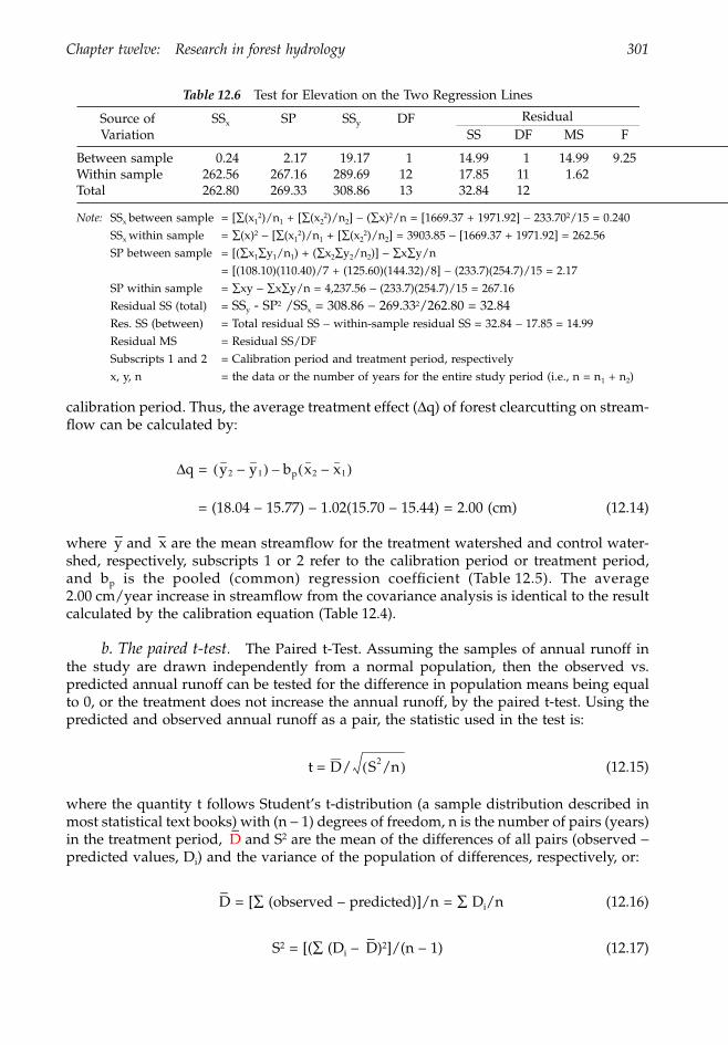
Chapter twelve: Research in forest hydrology 301
calibration period. Thus, the average treatment effect (Dq) of forest clearcutting on stream-flow can be calculated by:
Dq =
= (18.04 – 15.77) – 1.02(15.70 – 15.44) = 2.00 (cm) (12.14)
where –y and –x are the mean streamflow for the treatment watershed and control water-shed, respectively, subscripts 1 or 2 refer to the calibration period or treatment period,and bp is the pooled (common) regression coefficient (Table 12.5). The average2.00 cm/year increase in streamflow from the covariance analysis is identical to the resultcalculated by the calibration equation (Table 12.4).
b. The paired t-test. The Paired t-Test. Assuming the samples of annual runoff inthe study are drawn independently from a normal population, then the observed vs.predicted annual runoff can be tested for the difference in population means being equalto 0, or the treatment does not increase the annual runoff, by the paired t-test. Using thepredicted and observed annual runoff as a pair, the statistic used in the test is:
(12.15)
where the quantity t follows Student’s t-distribution (a sample distribution described inmost statistical text books) with (n - 1) degrees of freedom, n is the number of pairs (years)in the treatment period,
–D and S2 are the mean of the differences of all pairs (observed -
predicted values, Di) and the variance of the population of differences, respectively, or:
–D = [Â (observed – predicted)]/n = Â Di/n (12.16)
S2 = [(Â (Di ––D)2]/(n – 1) (12.17)
Table 12.6 Test for Elevation on the Two Regression Lines
Source of Variation
SSx SP SSy DF Residual SS DF MS F
Between sample 0.24 2.17 19.17 1 14.99 1 14.99 9.25Within sample 262.56 267.16 289.69 12 17.85 11 1.62Total 262.80 269.33 308.86 13 32.84 12
Note: SSx between sample = [Â(x12)/n1 + [Â(x2
2)/n2] - (Âx)2/n = [1669.37 + 1971.92] - 233.702/15 = 0.240 SSx within sample = Â(x)2 - [Â(x1
2)/n1 + [Â(x22)/n2] = 3903.85 - [1669.37 + 1971.92] = 262.56
SP between sample = [(Âx1Ây1/n1) + (Âx2Ây2/n2)] - ÂxÂy/n= [(108.10)(110.40)/7 + (125.60)(144.32)/8] - (233.7)(254.7)/15 = 2.17
SP within sample = Âxy - ÂxÂy/n = 4,237.56 - (233.7)(254.7)/15 = 267.16Residual SS (total) = SSy - SP2 /SSx = 308.86 - 269.332/262.80 = 32.84Res. SS (between) = Total residual SS - within-sample residual SS = 32.84 - 17.85 = 14.99Residual MS = Residual SS/DFSubscripts 1 and 2 = Calibration period and treatment period, respectivelyx, y, n = the data or the number of years for the entire study period (i.e., n = n1 + n2)
y2 – y1( ) bp x2 – x1( )–
t = D/ S2/n( )
1363_C12_fm Page 301 Wednesday, December 4, 2002 7:45 AM
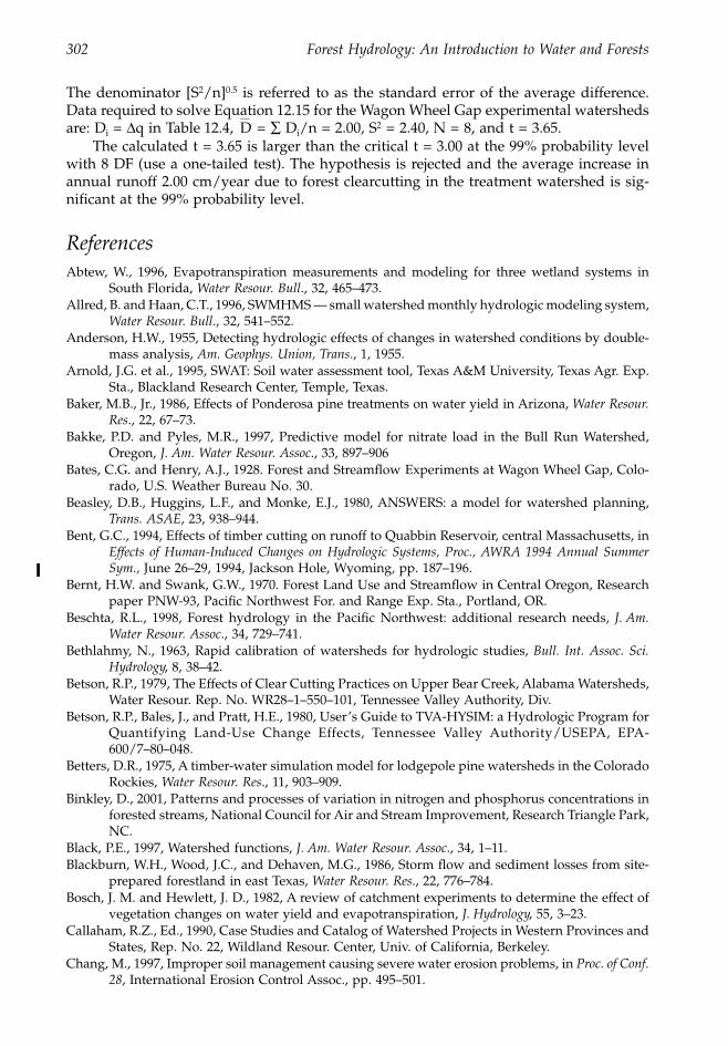
302 Forest Hydrology: An Introduction to Water and Forests
The denominator [S2/n]0.5 is referred to as the standard error of the average difference.Data required to solve Equation 12.15 for the Wagon Wheel Gap experimental watershedsare: Di = Dq in Table 12.4,`D = Â Di/n = 2.00, S2 = 2.40, N = 8, and t = 3.65.
The calculated t = 3.65 is larger than the critical t = 3.00 at the 99% probability levelwith 8 DF (use a one-tailed test). The hypothesis is rejected and the average increase inannual runoff 2.00 cm/year due to forest clearcutting in the treatment watershed is sig-nificant at the 99% probability level.
ReferencesAbtew, W., 1996, Evapotranspiration measurements and modeling for three wetland systems in
South Florida, Water Resour. Bull., 32, 465–473.Allred, B. and Haan, C.T., 1996, SWMHMS — small watershed monthly hydrologic modeling system,
Water Resour. Bull., 32, 541–552.Anderson, H.W., 1955, Detecting hydrologic effects of changes in watershed conditions by double-
mass analysis, Am. Geophys. Union, Trans., 1, 1955.Arnold, J.G. et al., 1995, SWAT: Soil water assessment tool, Texas A&M University, Texas Agr. Exp.
Sta., Blackland Research Center, Temple, Texas.Baker, M.B., Jr., 1986, Effects of Ponderosa pine treatments on water yield in Arizona, Water Resour.
Res., 22, 67–73.Bakke, P.D. and Pyles, M.R., 1997, Predictive model for nitrate load in the Bull Run Watershed,
Oregon, J. Am. Water Resour. Assoc., 33, 897–906Bates, C.G. and Henry, A.J., 1928. Forest and Streamflow Experiments at Wagon Wheel Gap, Colo-
rado, U.S. Weather Bureau No. 30. Beasley, D.B., Huggins, L.F., and Monke, E.J., 1980, ANSWERS: a model for watershed planning,
Trans. ASAE, 23, 938–944.Bent, G.C., 1994, Effects of timber cutting on runoff to Quabbin Reservoir, central Massachusetts, in
Effects of Human-Induced Changes on Hydrologic Systems, Proc., AWRA 1994 Annual SummerSym., June 26–29, 1994, Jackson Hole, Wyoming, pp. 187–196.
Bernt, H.W. and Swank, G.W., 1970. Forest Land Use and Streamflow in Central Oregon, Researchpaper PNW-93, Pacific Northwest For. and Range Exp. Sta., Portland, OR.
Beschta, R.L., 1998, Forest hydrology in the Pacific Northwest: additional research needs, J. Am.Water Resour. Assoc., 34, 729–741.
Bethlahmy, N., 1963, Rapid calibration of watersheds for hydrologic studies, Bull. Int. Assoc. Sci.Hydrology, 8, 38–42.
Betson, R.P., 1979, The Effects of Clear Cutting Practices on Upper Bear Creek, Alabama Watersheds,Water Resour. Rep. No. WR28–1–550–101, Tennessee Valley Authority, Div.
Betson, R.P., Bales, J., and Pratt, H.E., 1980, User’s Guide to TVA-HYSIM: a Hydrologic Program forQuantifying Land-Use Change Effects, Tennessee Valley Authority/USEPA, EPA-600/7–80–048.
Betters, D.R., 1975, A timber-water simulation model for lodgepole pine watersheds in the ColoradoRockies, Water Resour. Res., 11, 903–909.
Binkley, D., 2001, Patterns and processes of variation in nitrogen and phosphorus concentrations inforested streams, National Council for Air and Stream Improvement, Research Triangle Park,NC.
Black, P.E., 1997, Watershed functions, J. Am. Water Resour. Assoc., 34, 1–11.Blackburn, W.H., Wood, J.C., and Dehaven, M.G., 1986, Storm flow and sediment losses from site-
prepared forestland in east Texas, Water Resour. Res., 22, 776–784.Bosch, J. M. and Hewlett, J. D., 1982, A review of catchment experiments to determine the effect of
vegetation changes on water yield and evapotranspiration, J. Hydrology, 55, 3–23.Callaham, R.Z., Ed., 1990, Case Studies and Catalog of Watershed Projects in Western Provinces and
States, Rep. No. 22, Wildland Resour. Center, Univ. of California, Berkeley.Chang, M., 1997, Improper soil management causing severe water erosion problems, in Proc. of Conf.
28, International Erosion Control Assoc., pp. 495–501.
1363_C12_fm Page 302 Wednesday, December 4, 2002 7:45 AM
Chapter twelve: Research in forest hydrology 303
Chang, M. and Boyer, D.G., 1977, Estimates of low flows using watershed and climatic parameters,Water Resour. Res., 13, 997–1001.
Chang, M. and Crowley, C.M., 1997, Downstream effects of a dammed reservoir on streamflow andvegetation in east Texas, in Sustainability of Water Resources under Increasing Uncertainty,Rosbjerg, D., et al., Eds., IAHS Publ. No. 240, pp. 267–275.
Chang, M. and Lee, R., 1974, Objective double-mass analysis, Water Resour. Res., 10, 1123–1126.Chang, M. et al., 1997, Evapotranspiration of herbaceous mimosa (Mimosa strigillosa), a new drought-
resistant species in the southeastern United States, Resour., Conserv. Recycling, 21, 175–184.Chang, M. and Sayok, A.K., 1990, Hydrological responses to urbanization in forested La Nana Creek
watershed, Nacogdoches, Texas, in Tropical Hydrology and Caribbean Water Resources, Proc.,Am. Water Resour. Assoc., pp.131–40.
Chang, M. and Ting, J.C., 1986, Applications of the universal soil loss equation to various forestconditions, in Monitoring to Detect Changes in Water Quality Series (Proc. of the Budapest Sym,July 1986), IAHS, pp. 165–174.
Chang, M. and Waters, S.P., 1984, Forests and other factors associated with streamflows in east Texas,Water Resour. Bull., 20, 713–719.
Clayton, J.L. and Megahan, W.F., 1997, Natural erosion rates and their prediction in the IdahoBatholith, J. Am. Water Resour. Assoc., 33, 689–703.
Cooter, E.J. et al., 1993, General Circulation Model Output for Forest Climate Change Research andApplications, Gen. Tech. Rep. SE-85, U.S. Forest Service, SE For. Exp. Sta., Asheville, NC.
Crawford, N.H. and Linsley, R.K., 1966, Digital Simulation Hydrology: Stanford Water-shed Model4, Tech. Rep. 39, Stanford University, Dept. of Civil Eng., Stanford, CA.
Davis, E.A., 1993, Chaparral control in mosaic pattern increased streamflow and mitigated nitrateloss in Arizona, Water Resour. Bull., 29, 391–399.
DeCoursey, D.G. and Deal, R.B., 1971, General aspects of multivariate analysis with applications tosome problems in hydrology, in Proc. Sym. on Statistical Hydrology, USDA, Agr. Res. Service,Misc. Publ. No. 1275, pp. 47–68.
Douglas, J.E., 1967, Effects of species and arrangement of forests on evapo-transpiration, in Interna-tional Symp. on Forest Hydrology, Sopper, W.E. and Lull, H.W., Eds., Pergamon Press, Elmsford,NY, pp. 451–461.
Douglas, J.E., 1983, The potential for water yield augmentation from forest management in theeastern United States, Water Resources Bull., 19, 351–358.
EPA, 1997, Monitoring Guidance for Determining the Effectiveness of Nonpoint Source Controls,EPA 841-B-96–004, U.S. Environ. Protection Agency, Washington, D.C.
Foster, G.R. and Lane, L.J., 1987, User requirements USDA-Water Erosion Prediction Project (WEEP),NSERL Report No. 1, National Soil Erosion Research Laboratory, West Lafayette, IN.
Forest Service, 1977, Non-Point Water Quality Modeling in Wildland Management: A State-of-the-Art Assessment, Vol. II, EPA-600/3–77–078.
Friedrich, W., 1967, Forest hydrology research in Germany F.R, in International Sym. on Forest Hy-drology, Sopper, W.E. and Lull, H.W., Eds., Pergamon Press, Elmsford, NY.
Galbraith, A.F., 1975, Methods for predicting increases in water yield related to timber harvestingand site conditions, in Proc. Watershed Management, ASCE, New York, pp. 169–184.
Gary, H.L., 1975, Watershed Management Problems and Opportunities for the Colorado Front RangePonderosa Pine Zone: the Status of our Knowledge, Res. Paper RM-139, USDA Forest Service,Rocky Mountain Forest and Range Exp. Sta., Fort Collins, CO.
Gary, H.L. and Troendle, C.A., 1982, Snow accumulation and melt under various stand density inlodgepole pine in Wyoming and Colorado, Res. Note RM-417, U.S. Forest Service, RockyMountain Forest and Range Exp. Sta., Fort Collins, CO.
Gluns, D.R. and Toews, D.A.A., 1989, Effect of a major wildlife on water quality in southeasternBritish Columbia, in Sym. Proc. Headwaters Hydrology, Woessner, W.W. and Potts, D.F., Eds.,Am. Water Resour. Assoc., pp. 487–499.
Harr, R.D., 1983, Potential for augmenting water yield through forest practices in western Washing-ton and western Oregon, Water Resour. Bull., 19, 383–394.
1363_C12_fm Page 303 Wednesday, December 4, 2002 7:45 AM
304 Forest Hydrology: An Introduction to Water and Forests
Harr, R.D., Fredriksen, R.L., and Rothacher, J., 1979, Changes in streamflow following timber harvestin Southwest Oregon, Res. Paper PNW-249, Pacific Northwest Forest and Range Exp. Sta.,Forest Service.
Harrold, L.L. and Dreibelbis, F.R., 1958, Evaluation of Agricultural Hydrology by Monolith Lysim-eters, U.S. Dept. Agr. Tech. Bull. #1179,U.S. Govern. Printing Office, Washington, D.C.
Haupt, H.F., 1979, Effects of Timber Cutting and Revegetation on Snow Accumulation and Melt inNorth Idaho, Res. Paper INT-224, USDA Forest Service, Intermountain Forest and RangeExp. Sta., Ogden, UT.
Hewlett, J.D., 1970, Review of the catchment experiment to determine water yield, Proc. Joint U.N.Food Agr. Organ. — USSR, Intern’l Symp. Forest Influences and Watershed Management, Moscow,USSR. August – Sept., 1970, pp.145–155.
Hewlett, J.D., 1971, Comments on the catchment to determine vegetal effects on water yield, WaterResour. Bull., 7, 376–377.
Hewlett, J.D. and Hibbert, A.R., 1961, Increases in water yield after several types of forest cutting,Int. Assoc. Sci. Hydro. Bull., 6, 5–17.
Hewlett, J.D., Lull, H.W., and Reinhart, K.G., 1969, In defense of experimental watersheds, WaterResour. Res., 5, 306–316.
Hibbert, A.R., 1981, Opportunity to increase water yield in the southwest by vegetation management,in Interior West Watershed Management, Symp. Proc., Washington State University, Pullman,WA, pp. 223–230.
Hibbert, A.R., Davis, E.A., and Knipe, O.D. 1982, Water yield changes resulting from treatment ofArizona chaparral, in Proc. of Sym. on Dynamic and Management of Mediterranean-Type Ecosys-tems, June 22–26, 1981, San Diego. Cal., General Tech. Rep. PSW-58, U.S. Forest Service, PacificSW Forest and Range Exp. Sta., Berkeley, CA, pp. 382–389.
Hibbert, A.R., Knipe, O.D., and Davis, E.A., 1986, Streamflow response to control of chaparral shrubsalong channels and upper slopes, in Proc., Chaparral Ecosystems Research Conference, May16–17, 1985, Santa Barbara, Cal., University of California, Davis, Rep. No. 62, pp.95–103.
Hillman, G.R. and Verschuren, J.P., 1988, Simulation of the effects of forest cover, and its removal,on subsurface water, Water Resour. Res., 24, 305–314.
Hoover, M.D., 1944, Effect of removal of forest vegetation upon water yields, Trans. Am. Geophys.Union, 26, 969–975.
Hornbeck, J.W. et al., 1987, The northern hardwood forest ecosystem: ten years of recovery fromclearcutting, USDA, Forest Service, Northeastern Forest Exp. Sta., NE-RP-596.
Idso, S.B., Reginato, R.J., and Jackson, R.D., 1979, Calculation of evaporation during three stages ofsoil drying, Water Resour. Res., 15, 487–488.
Jaynes, R.A., 1975, A hydrologic model of aspen-conifer succession in the western United States,Res. Paper INT-213, Intermountain For. and Range Exp. Sta.,Ogden, UT.
Johnson, E.A. and Kovner, J.L., 1954, Increasing water yield by cutting forest vegetation, GeorgiaMiner. Newsl., 7, 145–148.
Kennedy, J.B., and Neville, A.M., 1986, Basic Statistical Methods for Engineers and Scientists, 3rd ed.,Harper & Row, New York.
Keppeler, E.T. and Ziemer, R.R., 1990, Logging effects on streamflow: water yield and summer lowflows at Caspar Creek in northwestern California, Water Resour. Res., 26, 1669–1679.
Kirkham, R.R., Gee, G.W., and Jones, T.L., 1984. Weighing lysimeters for long-term water balanceinvestigations at remote sites, Soil Sci. Soc. Am. J, 48, 1203–1205.
Knisel, W.G., 1980, CREAMS: a Field-Scale Model for Chemicals, Runoff, and Erosion from Agri-cultural Management Systems, Conserv. Res. Report No. 26, USDA Sci. and Education Ad-min.
Kochenderfer, J.M. and Aubertin, G.M., 1975, Effects of management practices on water quality andquantity: Fernow Experimental Forest, West Virginia, in Municipal Watershed Management,Symp. Proc., U.S. Forest Serv. Gen. Tech. Rep. NE-13, pp. 14–24.
Kochenderfer, J.N. and Wendel, G.W., 1983, Plant succession and hydrologic recovery on a deforestedand herbicided watershed, For. Sci., 29, 545–558.
Kovner, J.L. and Evans, T.C., 1954, A method for determining the minimum duration of watershedexperiments, Trans. Am. Geophys. Union, 35, 608–612.
1363_C12_fm Page 304 Wednesday, December 4, 2002 7:45 AM
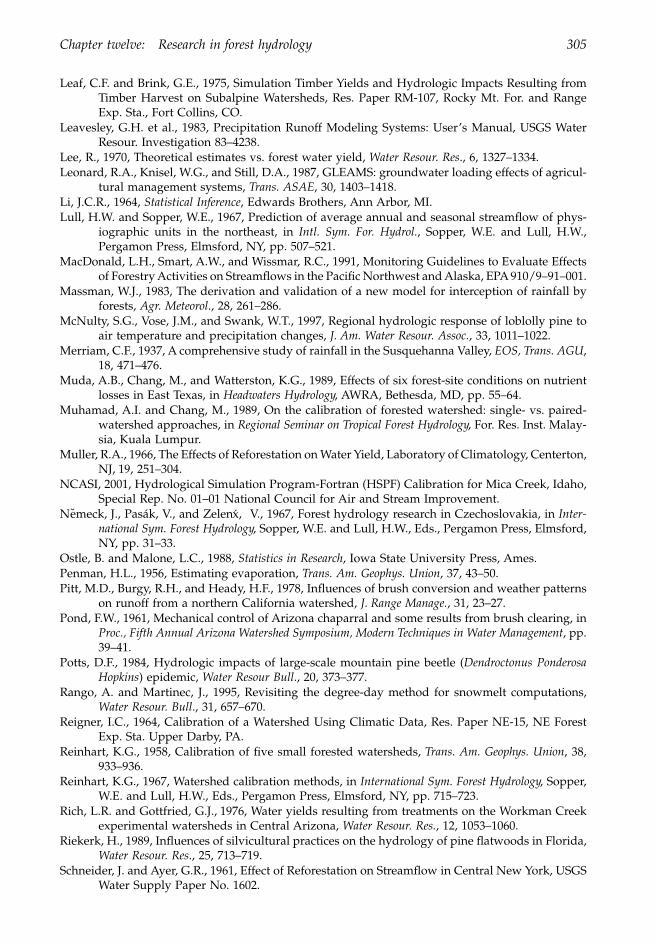
Chapter twelve: Research in forest hydrology 305
Leaf, C.F. and Brink, G.E., 1975, Simulation Timber Yields and Hydrologic Impacts Resulting fromTimber Harvest on Subalpine Watersheds, Res. Paper RM-107, Rocky Mt. For. and RangeExp. Sta., Fort Collins, CO.
Leavesley, G.H. et al., 1983, Precipitation Runoff Modeling Systems: User’s Manual, USGS WaterResour. Investigation 83–4238.
Lee, R., 1970, Theoretical estimates vs. forest water yield, Water Resour. Res., 6, 1327–1334.Leonard, R.A., Knisel, W.G., and Still, D.A., 1987, GLEAMS: groundwater loading effects of agricul-
tural management systems, Trans. ASAE, 30, 1403–1418.Li, J.C.R., 1964, Statistical Inference, Edwards Brothers, Ann Arbor, MI.Lull, H.W. and Sopper, W.E., 1967, Prediction of average annual and seasonal streamflow of phys-
iographic units in the northeast, in Intl. Sym. For. Hydrol., Sopper, W.E. and Lull, H.W.,Pergamon Press, Elmsford, NY, pp. 507–521.
MacDonald, L.H., Smart, A.W., and Wissmar, R.C., 1991, Monitoring Guidelines to Evaluate Effectsof Forestry Activities on Streamflows in the Pacific Northwest and Alaska, EPA 910/9–91–001.
Massman, W.J., 1983, The derivation and validation of a new model for interception of rainfall byforests, Agr. Meteorol., 28, 261–286.
McNulty, S.G., Vose, J.M., and Swank, W.T., 1997, Regional hydrologic response of loblolly pine toair temperature and precipitation changes, J. Am. Water Resour. Assoc., 33, 1011–1022.
Merriam, C.F., 1937, A comprehensive study of rainfall in the Susquehanna Valley, EOS, Trans. AGU,18, 471–476.
Muda, A.B., Chang, M., and Watterston, K.G., 1989, Effects of six forest-site conditions on nutrientlosses in East Texas, in Headwaters Hydrology, AWRA, Bethesda, MD, pp. 55–64.
Muhamad, A.I. and Chang, M., 1989, On the calibration of forested watershed: single- vs. paired-watershed approaches, in Regional Seminar on Tropical Forest Hydrology, For. Res. Inst. Malay-sia, Kuala Lumpur.
Muller, R.A., 1966, The Effects of Reforestation on Water Yield, Laboratory of Climatology, Centerton,NJ, 19, 251–304.
NCASI, 2001, Hydrological Simulation Program-Fortran (HSPF) Calibration for Mica Creek, Idaho,Special Rep. No. 01–01 National Council for Air and Stream Improvement.
Nemeck, J., Pasák, V., and Zelenx, V., 1967, Forest hydrology research in Czechoslovakia, in Inter-national Sym. Forest Hydrology, Sopper, W.E. and Lull, H.W., Eds., Pergamon Press, Elmsford,NY, pp. 31–33.
Ostle, B. and Malone, L.C., 1988, Statistics in Research, Iowa State University Press, Ames.Penman, H.L., 1956, Estimating evaporation, Trans. Am. Geophys. Union, 37, 43–50.Pitt, M.D., Burgy, R.H., and Heady, H.F., 1978, Influences of brush conversion and weather patterns
on runoff from a northern California watershed, J. Range Manage., 31, 23–27.Pond, F.W., 1961, Mechanical control of Arizona chaparral and some results from brush clearing, in
Proc., Fifth Annual Arizona Watershed Symposium, Modern Techniques in Water Management, pp.39–41.
Potts, D.F., 1984, Hydrologic impacts of large-scale mountain pine beetle (Dendroctonus PonderosaHopkins) epidemic, Water Resour Bull., 20, 373–377.
Rango, A. and Martinec, J., 1995, Revisiting the degree-day method for snowmelt computations,Water Resour. Bull., 31, 657–670.
Reigner, I.C., 1964, Calibration of a Watershed Using Climatic Data, Res. Paper NE-15, NE ForestExp. Sta. Upper Darby, PA.
Reinhart, K.G., 1958, Calibration of five small forested watersheds, Trans. Am. Geophys. Union, 38,933–936.
Reinhart, K.G., 1967, Watershed calibration methods, in International Sym. Forest Hydrology, Sopper,W.E. and Lull, H.W., Eds., Pergamon Press, Elmsford, NY, pp. 715–723.
Rich, L.R. and Gottfried, G.J., 1976, Water yields resulting from treatments on the Workman Creekexperimental watersheds in Central Arizona, Water Resour. Res., 12, 1053–1060.
Riekerk, H., 1989, Influences of silvicultural practices on the hydrology of pine flatwoods in Florida,Water Resour. Res., 25, 713–719.
Schneider, J. and Ayer, G.R., 1961, Effect of Reforestation on Streamflow in Central New York, USGSWater Supply Paper No. 1602.
1363_C12_fm Page 305 Wednesday, December 4, 2002 7:45 AM
306 Forest Hydrology: An Introduction to Water and Forests
Searcy, C.F. and Hardison, C.H., 1960, Double-Mass Curves, Water Supply Paper 1541-B, U.S. Geo-logical Survey, pp. 27–66.
Shahlaee, A.K. et al., 1991, Runoff and sediment production from burned forested sites in the GeorgiaPiedmont, Water Resour. Bull., 27, 485–493.
Shuttleworth, W.J., 1993, Evaporation, in Handbook of Hydrology, Maidment, D.R., Ed., McGraw-Hill,New York, pp. 4.1–4.53.
Stegman, S.V., 1996, Snowpack changes resulting from timber harvest: interception, redistribution,and evaporation, Water Resour. Bull., 32, 1353–1360.
Stewart, J.B., 1984, Measurement and prediction of evaporation from forested and agriculturalwatersheds, Agr. Water Manage., 8, 1–28.
Swanson, R.H., 1998, Forest hydrology issues for the 21st century: a consultant’s viewpoint, J. Am.Water Resour. Assoc., 34, 755–763.
Thornthwaite, C.W. and Mather, J.R., 1955. The Water Balance. Laboratory of Climatology, DrexelInst. Tech., Publ. Climatology, 8, No. 1, 104 pp.
Thornthwaite, C.W. and Mather, J.R., 1957, Instruction and Tables for Computing Potential Evapo-transpiration and the Water Balance, Laboratory of Climatology XIX (3), Centerton, NJ,pp.185–311.
Troendle, C.A. and King, R.M., 1985, The effect of timber harvest on the Fool Creek watershed, 30years later, Water Resour. Res., 21, 1915–1922.
Troendle, C.A. and King, R.M., 1987, The effect of partial and clearcutting on streamflow at Dead-horse Creek, Colorado, J. Hydrology, 90, 145–157.
TVA, 1961, Forest Cover Improvement Influences upon Hydrologic Characteristics of White HollowWatershed 1935–58, Rep. No. 0–5163A, Div. Water Control Planning, Tennessee Valley Au-thority, Cookeville, TN.
Ursic, SJ., 1991a, Hydrologic effects of two methods of harvesting mature southern pine, WaterResour. Bull., 27, 303–315.
Ursic, S.J., 1991b, Hydrologic effects of clearcutting and stripcutting loblolly pine in the CoastalPlain, Water Resour. Bull., 27, 925–938.
Ursic, S.J. and Popham, T.W., 1967, Using runoff events to calibrate small forested catchments, inProc. International Union of Forestry Res. Organizations Congress, pp. 319–324.
Veihmeyer, F.J., 1953, Use of water by native vegetation vs. grasses and forbs on watersheds, Trans.Am. Geophys. Union, 34, 201–212.
Ward, R.C., 1971, Small Watershed Experiments — An Appraisal of Concepts and Research Devel-opments, Occasional Papers in Geography No. 19, University of Hull, England.
Whittemore, R.C. and Beebe, J., 2000, EPA’s BASINS model: good science or serendipitous modeling?J. Am. Water Resour. Assoc., 36, 493–499.
Wight, J.R., 1987, ERHYM-II: Model Description and User Guide for the Basic Version, USDA, Agr.Res. Service, ARS 59.
Wight, J.R. and Skiles, J.W., Eds., 1987, SPUR: Simulation of Production and Utilization of Range-lands. Documentation and User Guide, USDA, Agr. Res. Service, ARS 63.
Wigmosta, M.S., Vail, L.W., and Lettenmaier, D.P, 1994, A distributed hydrology–soil–vegetationmodel for complex terrain, Water Resour. Res., 30, 1665–1679.
Williams, J.R., Nicks, A.D., and Arnold, J.G., 1985, Simulator for water resources in rural basins,J. Hydraulic Eng., 111, 970–986.
Williams, J.R., Jones, C.A., and Dyke, P.T., 1984, A modeling approach to determining the relationshipbetween erosion and soil productivity, Trans. ASAE 27, 1, 129–144.
Wilm, H.G., 1949, How long should experimental watersheds be calibrated? Trans. Am. Geophy.Union, 30, 272–278.
Young, R.A. et al., 1987, AGNPS, Agricultural Nonpoint Sources Pollution Model: A Large WatershedAnalysis Tool, Conser. Res. Report No. 35, USDA Agr. Res. Service.
1363_C12_fm Page 306 Wednesday, December 4, 2002 7:45 AM
307
Appendix A
Precipitation measurements
Contents
I. Precipitation gages ..........................................................................................................308A. Nonrecording gages ...............................................................................................308B. Recording gages ......................................................................................................309C. Storage gages...........................................................................................................310
II. Accuracy ...........................................................................................................................310A. Sources of error .......................................................................................................310B. Wind effects .............................................................................................................311C. “True” Precipitation................................................................................................311
III. Measurements..................................................................................................................311A. Gage installation .....................................................................................................311B. Improvements..........................................................................................................312
1. Shielded gages...................................................................................................3122. Pit gages .............................................................................................................3133. Tilted gages ........................................................................................................3134. Lysimeters ..........................................................................................................3135. Wind-speed adjustment ...................................................................................3136. Spherical gages..................................................................................................3137. Globoscopic pictures ........................................................................................315
References .....................................................................................................................................316
Measurements of precipitation are conventionally made by precipitation gages installedat specific sites (point measurements), and measurements from single gages are thenemployed to estimate average precipitation for the watershed. Thus, the reliability ofwatershed-precipitation estimates depends on the accuracy of point-precipitation mea-surements and the areal representativeness of each measurement. Precipitation gagesprovide the prime data used in watershed hydrologic studies. Other modern techniquessuch as radar observations (Creutin et al., 1988), satellite (Weng et al., 1994), and under-water ambient noises (Nystuen, 1986) are used to estimate areal precipitation from 1 km
2
to the entire continent and beyond. However, these techniques require ground validationand are generally used for weather and flood forecasts. This appendix discusses only thetechnique and accuracy of point-precipitation measurements.
1363_ AppA_fm Page 307 Wednesday, December 4, 2002 7:46 AM

308 Forest Hydrology: An Introduction to Water and Forests
I. Precipitation gages
The first known measurement of rainfall in history is believed to be in India, where bowlsas wide as 18 in. (45.72 cm) were set in the open to catch rainfall as a basis for land taxationas early as 400 B.C. (Kurtyka, 1953). In China, local county officers were asked to reportthe amount of rainfall measured between the vernal equinox (March 21) and the autumnalequinox (September 23) to the monarchal government during the East Hann dynasty,about 25 A.D. In the South Sung dynasty (1127–1279), a network of rain gages was set upat cities in all provinces. Several designs of rain gages were reported in 1241. One of therain gages measured 2 to 3 chih (old Chinese length scale, close to a foot) for the orificediameter, 1.2 chih for the bottom diameter, and 1.8 chih in depth (Liu, 1983). The Chineserain gages were earlier than the first rain gage designed by B. Castelli in 1639 in Europe(Kurtyka, 1953) by as much as 400 years.
Precipitation gages in use today are of three types: nonrecording, recording, andstorage gages.
A. Nonrecording gages
The basic design of nonrecording precipitation gages is an open cylinder with a sealedbottom installed in the open. Precipitation falling into the cylinder is collected and man-ually measured in terms of depth. However, the diameter of opening (orifice), the depthof cylinder (collector), the gage height above the ground, and the way that precipitationdepth is measured are different among countries. Sevruk and Klemn (1989) listed 50different types of nonrecording precipitation gages in use around the world today. A fewgages are given in Table A.1. Nonrecording gages are generally accepted as the standardin precipitation measurements.
Table A.1
A Few Standard Nonrecording Rain Gages in Use around the World
Country Gage Name Material Orifice Area(cm
2
)
Collector Depth(cm)
Gage Height
(cm)
Australia Manual 1508 Galvanized iron 324 7.0 30.0Brazil Ville Paris Stainless steel 400 13.0 63.0Canada Nipher Copper 127 50.0 52.0China China Galvanized iron 314 22.0 59.0France SPIEA MN Fiberglass 400 14.0 44.0Germany Hellman Galvanized iron 200 27.0 43.0Israel Small Hardened PVC 7 4.5 12.0Israel Amir Hardened PVC 100 8.0 50.0Malaysia S 203 DRG Brass 324 14.0 38.0Mexico Mexican Galvanized iron 400 15.0 36.0New Zealand Nylex 1000 Plastic 81 10.0 35.0U.K. Mark 2 Copper 127 15.0 30.0U.S. WB-8-inch Copper and steel 324 20.0 68.0Russia Tretjakov Galvanized iron 200 24.0 40.0Sweden SMHI Aluminum 200 15.0 35.0Switzerland Tognini Aluminum 200 27.0 43.0
Source:
After Sevruk, B. and Klemn, S., 1989, Types of standard precipitation gages, in
Precipitation Measurements
,Sevruk, B., Ed., WMO/IAHS/ETH Workshop, St. Moritz, Switzerland, pp. 227–232.
1363_ AppA_fm Page 308 Wednesday, December 4, 2002 7:46 AM
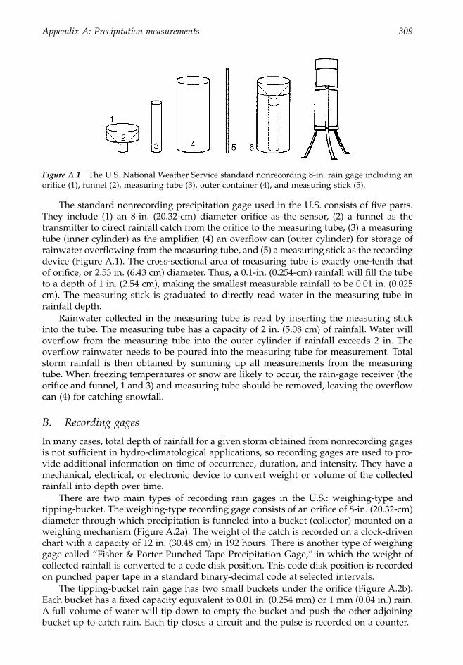
Appendix A: Precipitation measurements 309
The standard nonrecording precipitation gage used in the U.S. consists of five parts.They include (1) an 8-in. (20.32-cm) diameter orifice as the sensor, (2) a funnel as thetransmitter to direct rainfall catch from the orifice to the measuring tube, (3) a measuringtube (inner cylinder) as the amplifier, (4) an overflow can (outer cylinder) for storage ofrainwater overflowing from the measuring tube, and (5) a measuring stick as the recordingdevice (Figure A.1). The cross-sectional area of measuring tube is exactly one-tenth thatof orifice, or 2.53 in. (6.43 cm) diameter. Thus, a 0.1-in. (0.254-cm) rainfall will fill the tubeto a depth of 1 in. (2.54 cm), making the smallest measurable rainfall to be 0.01 in. (0.025cm). The measuring stick is graduated to directly read water in the measuring tube inrainfall depth.
Rainwater collected in the measuring tube is read by inserting the measuring stickinto the tube. The measuring tube has a capacity of 2 in. (5.08 cm) of rainfall. Water willoverflow from the measuring tube into the outer cylinder if rainfall exceeds 2 in. Theoverflow rainwater needs to be poured into the measuring tube for measurement. Totalstorm rainfall is then obtained by summing up all measurements from the measuringtube. When freezing temperatures or snow are likely to occur, the rain-gage receiver (theorifice and funnel, 1 and 3) and measuring tube should be removed, leaving the overflowcan (4) for catching snowfall.
B. Recording gages
In many cases, total depth of rainfall for a given storm obtained from nonrecording gagesis not sufficient in hydro-climatological applications, so recording gages are used to pro-vide additional information on time of occurrence, duration, and intensity. They have amechanical, electrical, or electronic device to convert weight or volume of the collectedrainfall into depth over time.
There are two main types of recording rain gages in the U.S.: weighing-type andtipping-bucket. The weighing-type recording gage consists of an orifice of 8-in. (20.32-cm)diameter through which precipitation is funneled into a bucket (collector) mounted on aweighing mechanism (Figure A.2a). The weight of the catch is recorded on a clock-drivenchart with a capacity of 12 in. (30.48 cm) in 192 hours. There is another type of weighinggage called “Fisher & Porter Punched Tape Precipitation Gage,” in which the weight ofcollected rainfall is converted to a code disk position. This code disk position is recordedon punched paper tape in a standard binary-decimal code at selected intervals.
The tipping-bucket rain gage has two small buckets under the orifice (Figure A.2b).Each bucket has a fixed capacity equivalent to 0.01 in. (0.254 mm) or 1 mm (0.04 in.) rain.A full volume of water will tip down to empty the bucket and push the other adjoiningbucket up to catch rain. Each tip closes a circuit and the pulse is recorded on a counter.
Figure A.1
The U.S. National Weather Service standard nonrecording 8-in. rain gage including anorifice (1), funnel (2), measuring tube (3), outer container (4), and measuring stick (5).
1363_ AppA_fm Page 309 Wednesday, December 4, 2002 7:46 AM
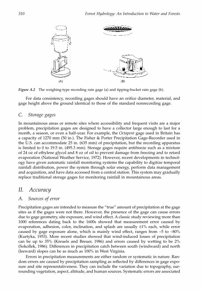
310 Forest Hydrology: An Introduction to Water and Forests
For data consistency, recording gages should have an orifice diameter, material, andgage height above the ground identical to those of the standard nonrecording gage.
C. Storage gages
In mountainous areas or remote sites where accessibility and frequent visits are a majorproblem, precipitation gages are designed to have a collector large enough to last for amonth, a season, or even a half-year. For example, the
Octapent
gage used in Britain hasa capacity of 1270 mm (50 in.). The Fisher & Porter Precipitation Gage-Recorder used inthe U.S. can accommodate 25 in. (635 mm) of precipitation, but the recording apparatusis limited to 0 to 19.5 in. (495.3 mm). Storage gages require antifreeze such as a mixtureof 24 oz of ethylene glycol and 8 oz of oil to prevent damage from freezing and to retardevaporation (National Weather Service, 1972). However, recent developments in technol-ogy have given automatic rainfall monitoring systems the capability to digitize temporalrainfall distribution, power the system through solar energy, perform data managementand acquisition, and have data accessed from a central station. This system may graduallyreplace traditional storage gages for monitoring rainfall in mountainous areas.
II. Accuracy
A. Sources of error
Precipitation gages are intended to measure the “true” amount of precipitation at the gagesites as if the gages were not there. However, the presence of the gage can cause errorsdue to gage geometry, site exposure, and wind effect. A classic study reviewing more than1000 references dating back to the 1600s showed that measurement error caused byevaporation, adhesion, color, inclination, and splash are usually
±
1% each, while errorcaused by gage exposure alone, which is mainly wind effect, ranges from
-
5 to
-
80%(Kurtyka, 1953). More recent studies showed that wind-induced losses of precipitationcan be up to 35% (Kreuels and Breuer, 1986) and errors caused by wetting to be 2%(Sokollek, 1986). Differences in precipitation catch between south (windward) and north(leeward) slopes can be as much as 100% in West Virginia.
Errors in precipitation measurements are either random or systematic in nature. Ran-dom errors are caused by precipitation sampling as reflected by differences in gage expo-sure and site representativeness. They can include the variation due to topography, sur-rounding vegetation, aspect, altitude, and human sources. Systematic errors are associated
Figure A.2
The weighing-type recording rain gage (a) and tipping-bucket rain gage (b).
1363_ AppA_fm Page 310 Wednesday, December 4, 2002 7:46 AM
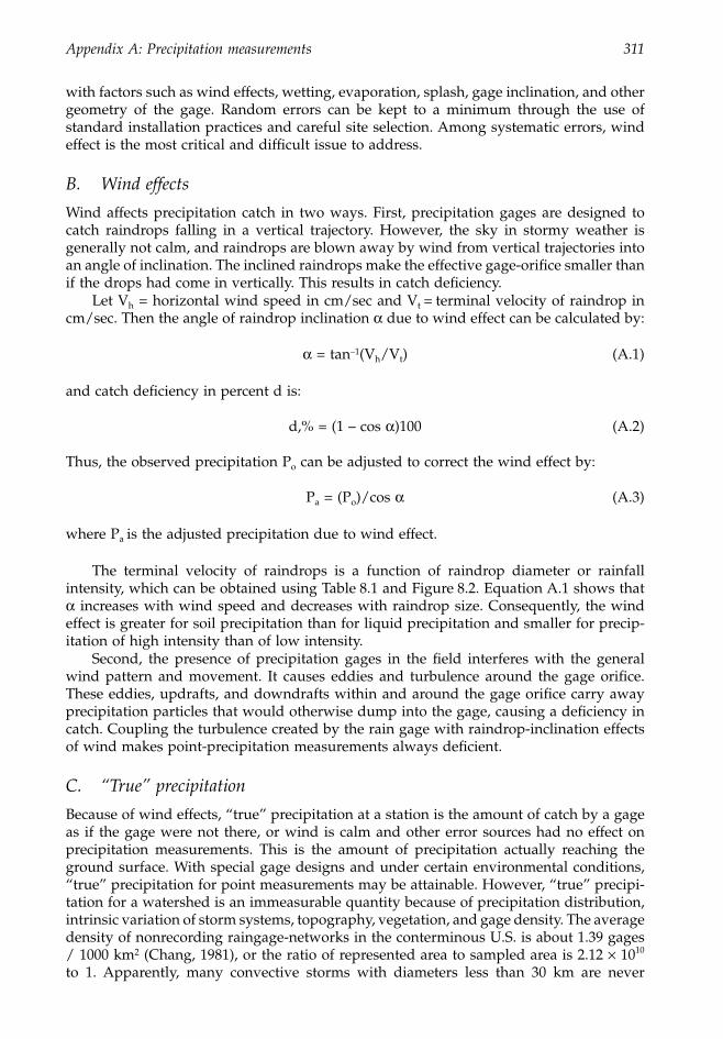
Appendix A: Precipitation measurements 311
with factors such as wind effects, wetting, evaporation, splash, gage inclination, and othergeometry of the gage. Random errors can be kept to a minimum through the use ofstandard installation practices and careful site selection. Among systematic errors, windeffect is the most critical and difficult issue to address.
B. Wind effects
Wind affects precipitation catch in two ways. First, precipitation gages are designed tocatch raindrops falling in a vertical trajectory. However, the sky in stormy weather isgenerally not calm, and raindrops are blown away by wind from vertical trajectories intoan angle of inclination. The inclined raindrops make the effective gage-orifice smaller thanif the drops had come in vertically. This results in catch deficiency.
Let V
h
= horizontal wind speed in cm/sec and V
t
=
terminal velocity of raindrop incm/sec. Then the angle of raindrop inclination
a
due to wind effect can be calculated by:
a
= tan
–1
(V
h
/V
t
) (A.1)
and catch deficiency in percent d is:
d,% = (1 – cos
a
)100 (A.2)
Thus, the observed precipitation P
o
can be adjusted to correct the wind effect by:
P
a
= (P
o
)/cos
a
(A.3)
where P
a
is the adjusted precipitation due to wind effect.
The terminal velocity of raindrops is a function of raindrop diameter or rainfallintensity, which can be obtained using Table 8.1 and Figure 8.2. Equation A.1 shows that
a
increases with wind speed and decreases with raindrop size. Consequently, the windeffect is greater for soil precipitation than for liquid precipitation and smaller for precip-itation of high intensity than of low intensity.
Second, the presence of precipitation gages in the field interferes with the generalwind pattern and movement. It causes eddies and turbulence around the gage orifice.These eddies, updrafts, and downdrafts within and around the gage orifice carry awayprecipitation particles that would otherwise dump into the gage, causing a deficiency incatch. Coupling the turbulence created by the rain gage with raindrop-inclination effectsof wind makes point-precipitation measurements always deficient.
C. “True” precipitation
Because of wind effects, “true” precipitation at a station is the amount of catch by a gageas if the gage were not there, or wind is calm and other error sources had no effect onprecipitation measurements. This is the amount of precipitation actually reaching theground surface. With special gage designs and under certain environmental conditions,“true” precipitation for point measurements may be attainable. However, “true” precipi-tation for a watershed is an immeasurable quantity because of precipitation distribution,intrinsic variation of storm systems, topography, vegetation, and gage density. The averagedensity of nonrecording raingage-networks in the conterminous U.S. is about 1.39 gages/ 1000 km
2
(Chang, 1981), or the ratio of represented area to sampled area is 2.12
¥
10
10
to 1. Apparently, many convective storms with diameters less than 30 km are never
1363_ AppA_fm Page 311 Wednesday, December 4, 2002 7:46 AM
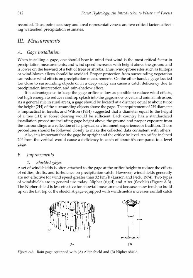
312 Forest Hydrology: An Introduction to Water and Forests
recorded. Thus, point accuracy and areal representativeness are two critical factors affect-ing watershed precipitation estimates.
III. Measurements
A. Gage installation
When installing a gage, one should bear in mind that wind is the most critical factor inprecipitation measurements, and wind speed increases with height above the ground andis lower on the leeward of a belt of trees or shrubs. Thus, wind-prone sites such as hilltopsor wind-blown alleys should be avoided. Proper protection from surrounding vegetationcan reduce wind effects on precipitation measurements. On the other hand, a gage locatedtoo close to surrounding objects or in a deep valley can cause a catch deficiency due toprecipitation interception and rain-shadow effect.
It is advantageous to keep the gage orifice as low as possible to reduce wind effects,but high enough to reduce raindrop splash into the gage, snow cover, and animal intrusion.As a general rule in rural areas, a gage should be located at a distance equal to about twicethe height (2H) of the surrounding objects above the gage. The requirement of 2H diameteris impractical in forests, and Wilson (1954) suggested that a diameter equal to the heightof a tree (1H) in forest clearing would be sufficient. Each country has a standardizedinstallation procedure including gage height above the ground and proper exposure fromthe surroundings as a reflection of its physical environment, experience, or tradition. Thoseprocedures should be followed closely to make the collected data consistent with others.
Also, it is important that the gage be upright and the orifice be level. An orifice inclined20
∞
from the vertical would cause a deficiency in catch of about 6% compared to a levelgage.
B. Improvements
1. Shielded gages
A set of windshields is often attached to the gage at the orifice height to reduce the effectsof eddies, drafts, and turbulence on precipitation catch. However, windshields generallyare not effective for wind speed greater than 32 km/h (Larson and Peck, 1974). Two typesof windshields are in general use today: Nipher (rigid) and Alter (flexible) (Figure A.3).The Nipher shield is less effective for snowfall measurement because snow tends to buildup on the flat top of the shield. A gage equipped with windshields increases rainfall catch
Figure A.3
Rain gage equipped with (A) Alter shield and (B) Nipher shield.
1363_ AppA_fm Page 312 Wednesday, December 4, 2002 7:46 AM
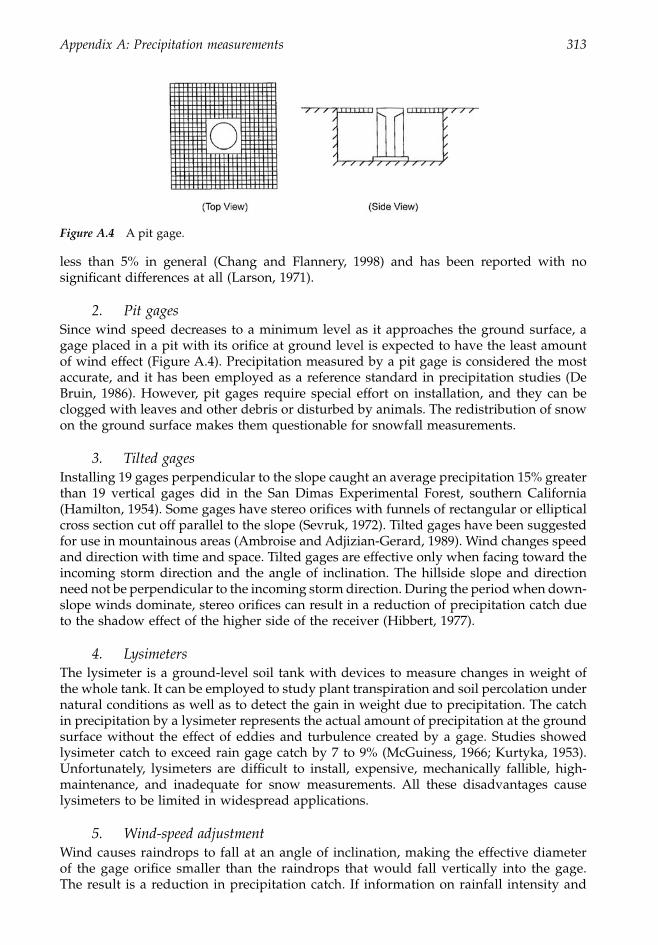
Appendix A: Precipitation measurements 313
less than 5% in general (Chang and Flannery, 1998) and has been reported with nosignificant differences at all (Larson, 1971).
2. Pit gages
Since wind speed decreases to a minimum level as it approaches the ground surface, agage placed in a pit with its orifice at ground level is expected to have the least amountof wind effect (Figure A.4). Precipitation measured by a pit gage is considered the mostaccurate, and it has been employed as a reference standard in precipitation studies (DeBruin, 1986). However, pit gages require special effort on installation, and they can beclogged with leaves and other debris or disturbed by animals. The redistribution of snowon the ground surface makes them questionable for snowfall measurements.
3. Tilted gages
Installing 19 gages perpendicular to the slope caught an average precipitation 15% greaterthan 19 vertical gages did in the San Dimas Experimental Forest, southern California(Hamilton, 1954). Some gages have stereo orifices with funnels of rectangular or ellipticalcross section cut off parallel to the slope (Sevruk, 1972). Tilted gages have been suggestedfor use in mountainous areas (Ambroise and Adjizian-Gerard, 1989). Wind changes speedand direction with time and space. Tilted gages are effective only when facing toward theincoming storm direction and the angle of inclination. The hillside slope and directionneed not be perpendicular to the incoming storm direction. During the period when down-slope winds dominate, stereo orifices can result in a reduction of precipitation catch dueto the shadow effect of the higher side of the receiver (Hibbert, 1977).
4. Lysimeters
The lysimeter is a ground-level soil tank with devices to measure changes in weight ofthe whole tank. It can be employed to study plant transpiration and soil percolation undernatural conditions as well as to detect the gain in weight due to precipitation. The catchin precipitation by a lysimeter represents the actual amount of precipitation at the groundsurface without the effect of eddies and turbulence created by a gage. Studies showedlysimeter catch to exceed rain gage catch by 7 to 9% (McGuiness, 1966; Kurtyka, 1953).Unfortunately, lysimeters are difficult to install, expensive, mechanically fallible, high-maintenance, and inadequate for snow measurements. All these disadvantages causelysimeters to be limited in widespread applications.
5. Wind-speed adjustment
Wind causes raindrops to fall at an angle of inclination, making the effective diameterof the gage orifice smaller than the raindrops that would fall vertically into the gage.The result is a reduction in precipitation catch. If information on rainfall intensity and
Figure A.4
A pit gage.
1363_ AppA_fm Page 313 Wednesday, December 4, 2002 7:46 AM
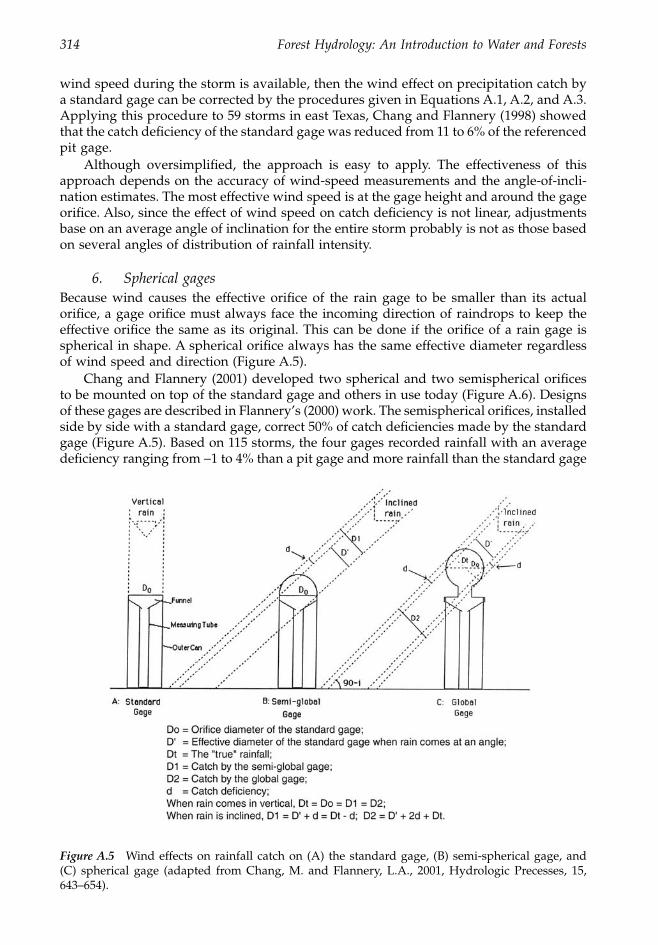
314 Forest Hydrology: An Introduction to Water and Forests
wind speed during the storm is available, then the wind effect on precipitation catch bya standard gage can be corrected by the procedures given in Equations A.1, A.2, and A.3.Applying this procedure to 59 storms in east Texas, Chang and Flannery (1998) showedthat the catch deficiency of the standard gage was reduced from 11 to 6% of the referencedpit gage.
Although oversimplified, the approach is easy to apply. The effectiveness of thisapproach depends on the accuracy of wind-speed measurements and the angle-of-incli-nation estimates. The most effective wind speed is at the gage height and around the gageorifice. Also, since the effect of wind speed on catch deficiency is not linear, adjustmentsbase on an average angle of inclination for the entire storm probably is not as those basedon several angles of distribution of rainfall intensity.
6. Spherical gages
Because wind causes the effective orifice of the rain gage to be smaller than its actualorifice, a gage orifice must always face the incoming direction of raindrops to keep theeffective orifice the same as its original. This can be done if the orifice of a rain gage isspherical in shape. A spherical orifice always has the same effective diameter regardlessof wind speed and direction (Figure A.5).
Chang and Flannery (2001) developed two spherical and two semispherical orificesto be mounted on top of the standard gage and others in use today (Figure A.6). Designsof these gages are described in Flannery’s (2000) work. The semispherical orifices, installedside by side with a standard gage, correct 50% of catch deficiencies made by the standardgage (Figure A.5). Based on 115 storms, the four gages recorded rainfall with an averagedeficiency ranging from
-
1 to 4% than a pit gage and more rainfall than the standard gage
Figure A.5
Wind effects on rainfall catch on (A) the standard gage, (B) semi-spherical gage, and(C) spherical gage (adapted from Chang, M. and Flannery, L.A., 2001, Hydrologic Precesses, 15,643–654).
1363_ AppA_fm Page 314 Wednesday, December 4, 2002 7:46 AM
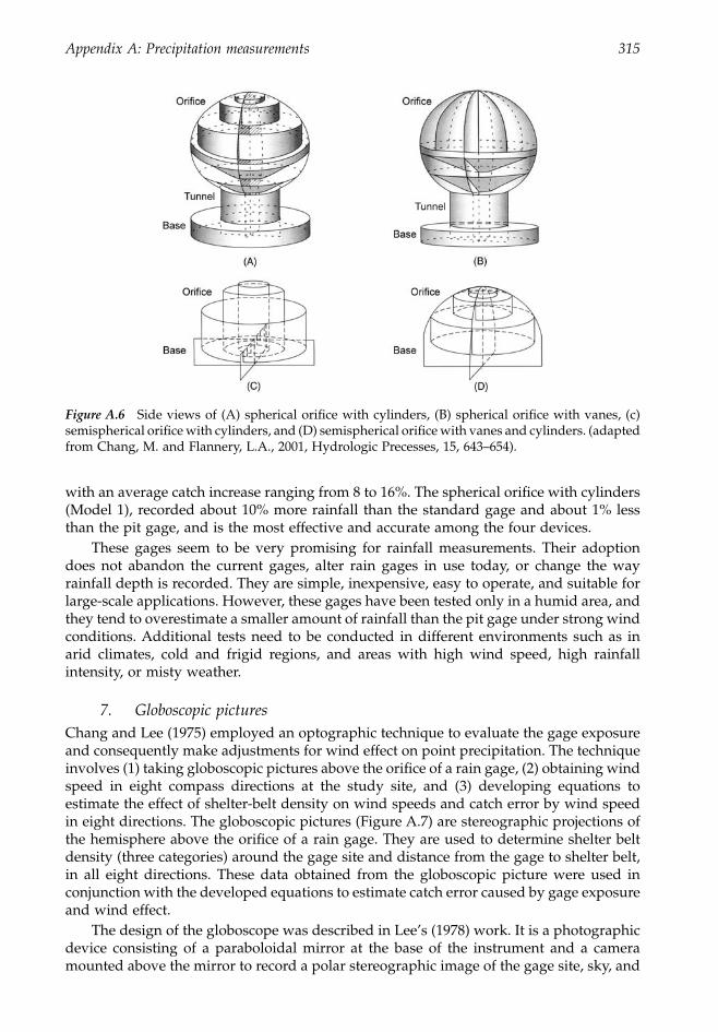
Appendix A: Precipitation measurements 315
with an average catch increase ranging from 8 to 16%. The spherical orifice with cylinders(Model 1), recorded about 10% more rainfall than the standard gage and about 1% lessthan the pit gage, and is the most effective and accurate among the four devices.
These gages seem to be very promising for rainfall measurements. Their adoptiondoes not abandon the current gages, alter rain gages in use today, or change the wayrainfall depth is recorded. They are simple, inexpensive, easy to operate, and suitable forlarge-scale applications. However, these gages have been tested only in a humid area, andthey tend to overestimate a smaller amount of rainfall than the pit gage under strong windconditions. Additional tests need to be conducted in different environments such as inarid climates, cold and frigid regions, and areas with high wind speed, high rainfallintensity, or misty weather.
7. Globoscopic pictures
Chang and Lee (1975) employed an optographic technique to evaluate the gage exposureand consequently make adjustments for wind effect on point precipitation. The techniqueinvolves (1) taking globoscopic pictures above the orifice of a rain gage, (2) obtaining windspeed in eight compass directions at the study site, and (3) developing equations toestimate the effect of shelter-belt density on wind speeds and catch error by wind speedin eight directions. The globoscopic pictures (Figure A.7) are stereographic projections ofthe hemisphere above the orifice of a rain gage. They are used to determine shelter beltdensity (three categories) around the gage site and distance from the gage to shelter belt,in all eight directions. These data obtained from the globoscopic picture were used inconjunction with the developed equations to estimate catch error caused by gage exposureand wind effect.
The design of the globoscope was described in Lee’s (1978) work. It is a photographicdevice consisting of a paraboloidal mirror at the base of the instrument and a cameramounted above the mirror to record a polar stereographic image of the gage site, sky, and
Figure A.6
Side views of (A) spherical orifice with cylinders, (B) spherical orifice with vanes, (c)semispherical orifice with cylinders, and (D) semispherical orifice with vanes and cylinders. (adaptedfrom Chang, M. and Flannery, L.A., 2001, Hydrologic Precesses, 15, 643–654).
1363_ AppA_fm Page 315 Wednesday, December 4, 2002 7:46 AM
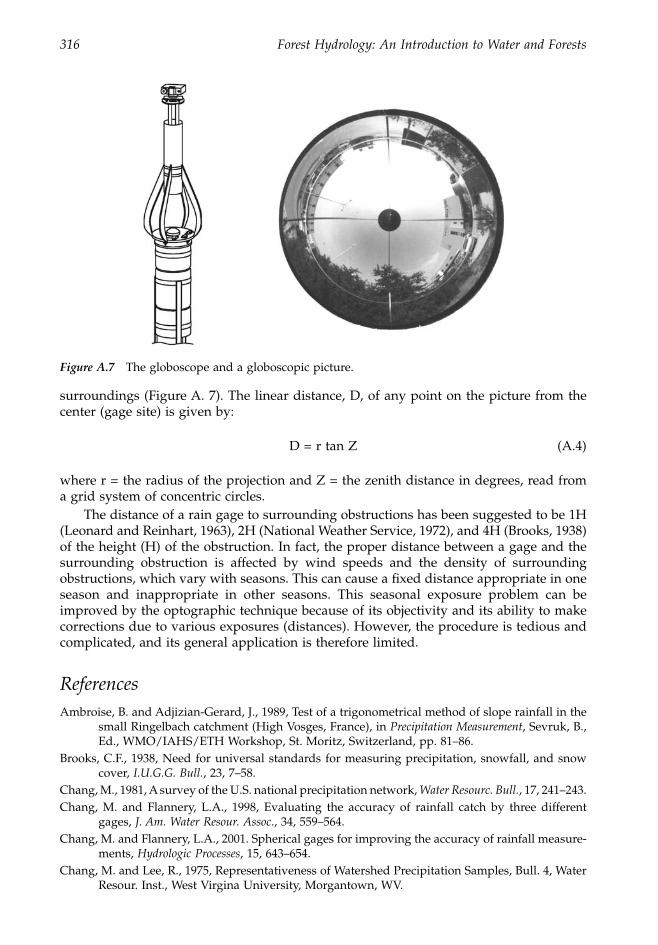
316 Forest Hydrology: An Introduction to Water and Forests
surroundings (Figure A. 7). The linear distance, D, of any point on the picture from thecenter (gage site) is given by:
D = r tan Z (A.4)
where r = the radius of the projection and Z = the zenith distance in degrees, read froma grid system of concentric circles.
The distance of a rain gage to surrounding obstructions has been suggested to be 1H(Leonard and Reinhart, 1963), 2H (National Weather Service, 1972), and 4H (Brooks, 1938)of the height (H) of the obstruction. In fact, the proper distance between a gage and thesurrounding obstruction is affected by wind speeds and the density of surroundingobstructions, which vary with seasons. This can cause a fixed distance appropriate in oneseason and inappropriate in other seasons. This seasonal exposure problem can beimproved by the optographic technique because of its objectivity and its ability to makecorrections due to various exposures (distances). However, the procedure is tedious andcomplicated, and its general application is therefore limited.
References
Ambroise, B. and Adjizian-Gerard, J., 1989, Test of a trigonometrical method of slope rainfall in thesmall Ringelbach catchment (High Vosges, France), in
Precipitation Measurement
, Sevruk, B.,Ed., WMO/IAHS/ETH Workshop, St. Moritz, Switzerland, pp. 81–86.
Brooks, C.F., 1938, Need for universal standards for measuring precipitation, snowfall, and snowcover,
I.U.G.G. Bull.
, 23, 7–58.Chang, M., 1981, A survey of the U.S. national precipitation network,
Water Resourc. Bull.
, 17, 241–243.Chang, M. and Flannery, L.A., 1998, Evaluating the accuracy of rainfall catch by three different
gages,
J. Am. Water Resour. Assoc
., 34, 559–564.Chang, M. and Flannery, L.A., 2001. Spherical gages for improving the accuracy of rainfall measure-
ments,
Hydrologic Processes
, 15, 643–654.Chang, M. and Lee, R., 1975, Representativeness of Watershed Precipitation Samples, Bull. 4, Water
Resour. Inst., West Virgina University, Morgantown, WV.
Figure A.7
The globoscope and a globoscopic picture.
1363_ AppA_fm Page 316 Wednesday, December 4, 2002 7:46 AM
Appendix A: Precipitation measurements 317
Creutin, J., Delrieu, G., and Lebel, T., 1988, Rainfall measurement by raingauge–radar combination:a geostatistical approach,
J. Atm. Ocean. Technol
., 5, 102–115.De Bruin, H.A.R., 1986, Results of the international comparison of rain gauges with a reference pit
gauge, part A: basic stations, in
Correction of Precipitation Measurements
, Sevruk, B., Ed.,ETH/IAHS/WMO Workshop, Zurich, Switzerland, pp. 97–100.
Flannery, L.A., 2000, Evaluating the Accuracy of Rainfall Measurements and Developing New Gagesfor Improvements, Unpublished MS Thesis, College of Forestry, Stephen F. Austin StateUniversity, Nacogdoches, TX.
Hamilton, E.L., 1954, Rainfall Sampling on Rugged Terrain, USDA Technical Bull. No. 1096.Hibbert, A.R., 1977. Distribution of precipitation on rugged terrain in Central Arizona,
HydrologyWater Resour. Arizona and the Southwest
, 7, 163–173.Kreuels, R.K. and Breuer, L.J., 1986, Wind influenced rain gage errors in heavy rain, in
Correction ofPrecipitation Measurements
, Sevruk, B., Ed., ETH/IAHS/WMO Workshop, Zurich, Switzer-land, pp. 105–107.
Kurtyka, J.C., 1953, Precipitation Measurements Study, Annual Report of Investigation No. 20, StateWater Survey Division, Urbana, IL.
Larson, L.W., 1971, Shielding Precipitation Gages from Adverse Wind Effects with Snow Fences,Water Resour. Series 25, Water Resour. Res. Inst., University of Wyoming, Laramie, WY, pp.1–161.
Larson, L.W. and Peck, E.L., 1974, Accuracy of precipitation measurements for hydrologic modeling,
Water Resour. Res
., 10, 857–863.Lee, R., 1978,
Forest Microclimatology
, Columbia University Press, New York.Leonard, R.E. and Reinhart, K.G., 1963, Some observations on precipitation measurement on forested
experimental watersheds, Res. Note NE-6, U.S. Forest Service, Northeastern Forest Exp. Sta.,Upper Darby, PA.
Liu, T.M., 1983, The inventories of meteorological instruments and observational equipment inancient China, in
The History of Chinese Technology
, Vol. II, Wu, T.L., Ed., The Natural Sciencesand Cultural Enterprises, Inc. Taipei, pp. 149–161. (In Chinese.)
McGuinness, J.L., 1966, A comparison of lysimeter catch and rain gage catch, USDA Agr. ResearchService ARS 41–124.
National Weather Service, 1972, Substation Observations, Supersedes Circular B, U.S. Dept. Com-merce, NOAA, Washington, D.C.
Nystuen, J.A., 1986, Rainfall measurements using underwater ambient noise,
J. Acoust. Soc. Am
., 79,972–982.
Sevruk, B., 1972, Precipitation measurements by means of storage gauges with stereo and horizontalorifices in the Baye De Montreux Watershed, in
Distribution of Precipitation in MountainousAreas
, Vol. II. WMO/OMM No. 326. Geneva, Switzerland, pp. 86–95.Sevruk, B. and Klemn, S., 1989. Types of standard precipitation gages, in
Precipitation Measurements
,Sevruk, B., Ed., WMO/IAHS/ETH Workshop, St. Moritz, Switzerland, pp. 227–232.
Sokollek, V., 1986, Problems of precipitation measurement for water budget studies in the Highlandsof Hessen, in
Correction of Precipitation Measurements
, Sevruk, B., Ed., ETH/IAHS/WMOWorkshop, Zurich, Switzerland, pp. 89–94.
Weng, F., Ferraro, R.R., and Grody, N.C., 1994, Global precipitation measurements using DMSP F-10 and F-11 Special Sensor Microwave Imager (SSM/I) data,
J. Geophys. Res.
, 99: 7423–7435.Wilson, W.T., 1954, Analysis of winter precipitation observations in cooperative snow investigation,
Mon. Weather Rev.
, 82, 183–195.
1363_ AppA_fm Page 317 Wednesday, December 4, 2002 7:46 AM

1363_ AppA_fm Page 318 Wednesday, December 4, 2002 7:46 AM
319
Appendix B
Streamflow measurements
Contents
I. River stage........................................................................................................................320A. Manual......................................................................................................................320B. Automatic.................................................................................................................320
II. Flow velocity....................................................................................................................322A. Velocity variation ....................................................................................................322B. Site selection ............................................................................................................322C. Methods....................................................................................................................322
1. Floats ...................................................................................................................3222. Velocity head .....................................................................................................3233. Current meters ..................................................................................................3244. Others..................................................................................................................324
a. Tracers...........................................................................................................325b. Hot-wire anemometers ..............................................................................325c. Electromagnetic method ............................................................................325d. Acoustic flowmeters ...................................................................................326e. Acoustic Doppler current profiler............................................................327
III. Discharge ..........................................................................................................................327A. Volumetric and gravimetric methods..................................................................327B. Velocity-area method..............................................................................................328C. Slope-area method ..................................................................................................328
IV. Stage–discharge relation ................................................................................................329A. Channel hydraulic geometry ................................................................................329B. The rating equation ................................................................................................331C. Precalibrated devices..............................................................................................332
1. Weirs....................................................................................................................333a. Features.........................................................................................................333b. Types of weirs .............................................................................................333c. Flow rates.....................................................................................................334
2. Flumes.................................................................................................................335a. Parshall flumes............................................................................................335b. Hs, H, and HL flumes................................................................................336
3. Orifices................................................................................................................338References .....................................................................................................................................339
1363_ AppB_fm Page 319 Wednesday, December 4, 2002 7:47 AM
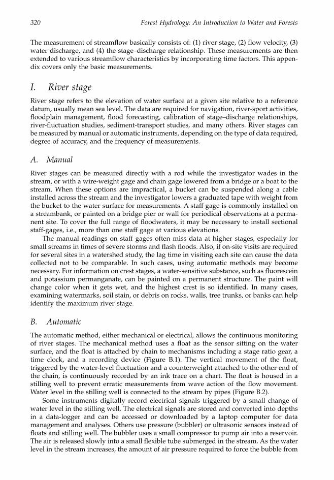
320 Forest Hydrology: An Introduction to Water and Forests
The measurement of streamflow basically consists of: (1) river stage, (2) flow velocity, (3)water discharge, and (4) the stage–discharge relationship. These measurements are thenextended to various streamflow characteristics by incorporating time factors. This appen-dix covers only the basic measurements.
I. River stage
River stage refers to the elevation of water surface at a given site relative to a referencedatum, usually mean sea level. The data are required for navigation, river-sport activities,floodplain management, flood forecasting, calibration of stage–discharge relationships,river-fluctuation studies, sediment-transport studies, and many others. River stages canbe measured by manual or automatic instruments, depending on the type of data required,degree of accuracy, and the frequency of measurements.
A. Manual
River stages can be measured directly with a rod while the investigator wades in thestream, or with a wire-weight gage and chain gage lowered from a bridge or a boat to thestream. When these options are impractical, a bucket can be suspended along a cableinstalled across the stream and the investigator lowers a graduated tape with weight fromthe bucket to the water surface for measurements. A staff gage is commonly installed ona streambank, or painted on a bridge pier or wall for periodical observations at a perma-nent site. To cover the full range of floodwaters, it may be necessary to install sectionalstaff-gages, i.e., more than one staff gage at various elevations.
The manual readings on staff gages often miss data at higher stages, especially forsmall streams in times of severe storms and flash floods. Also, if on-site visits are requiredfor several sites in a watershed study, the lag time in visiting each site can cause the datacollected not to be comparable. In such cases, using automatic methods may becomenecessary. For information on crest stages, a water-sensitive substance, such as fluoresceinand potassium permanganate, can be painted on a permanent structure. The paint willchange color when it gets wet, and the highest crest is so identified. In many cases,examining watermarks, soil stain, or debris on rocks, walls, tree trunks, or banks can helpidentify the maximum river stage.
B. Automatic
The automatic method, either mechanical or electrical, allows the continuous monitoringof river stages. The mechanical method uses a float as the sensor sitting on the watersurface, and the float is attached by chain to mechanisms including a stage ratio gear, atime clock, and a recording device (Figure B.1). The vertical movement of the float,triggered by the water-level fluctuation and a counterweight attached to the other end ofthe chain, is continuously recorded by an ink trace on a chart. The float is housed in astilling well to prevent erratic measurements from wave action of the flow movement.Water level in the stilling well is connected to the stream by pipes (Figure B.2).
Some instruments digitally record electrical signals triggered by a small change ofwater level in the stilling well. The electrical signals are stored and converted into depthsin a data-logger and can be accessed or downloaded by a laptop computer for datamanagement and analyses. Others use pressure (bubbler) or ultrasonic sensors instead offloats and stilling well. The bubbler uses a small compressor to pump air into a reservoir.The air is released slowly into a small flexible tube submerged in the stream. As the waterlevel in the stream increases, the amount of air pressure required to force the bubble from
1363_ AppB_fm Page 320 Wednesday, December 4, 2002 7:47 AM
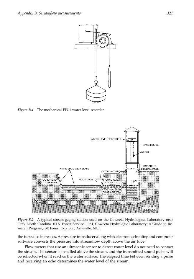
Appendix B: Streamflow measurements 321
the tube also increases. A pressure transducer along with electronic circuitry and computersoftware converts the pressure into streamflow depth above the air tube.
Flow meters that use an ultrasonic sensor to detect water level do not need to contactthe stream. The sensor is installed above the stream, and the transmitted sound pulse willbe reflected when it reaches the water surface. The elapsed time between sending a pulseand receiving an echo determines the water level of the stream.
Figure B.1
The mechanical FW-1 water-level recorder.
Figure B.2
A typical stream-gaging station used on the Coweeta Hydrological Laboratory nearOtto, North Carolina. (U.S. Forest Service, 1984, Coweeta Hydrologic Laboratory: A Guide to Re-search Program,
.
SE Forest Exp. Sta., Asheville, NC.)
1363_ AppB_fm Page 321 Wednesday, December 4, 2002 7:47 AM
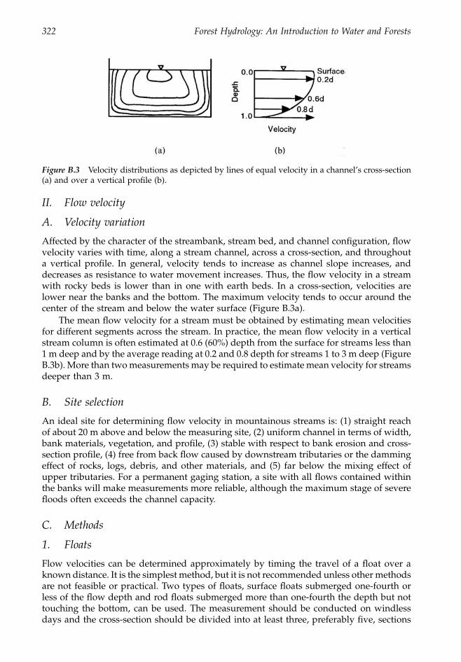
322 Forest Hydrology: An Introduction to Water and Forests
II. Flow velocity
A. Velocity variation
Affected by the character of the streambank, stream bed, and channel configuration, flowvelocity varies with time, along a stream channel, across a cross-section, and throughouta vertical profile. In general, velocity tends to increase as channel slope increases, anddecreases as resistance to water movement increases. Thus, the flow velocity in a streamwith rocky beds is lower than in one with earth beds. In a cross-section, velocities arelower near the banks and the bottom. The maximum velocity tends to occur around thecenter of the stream and below the water surface (Figure B.3a).
The mean flow velocity for a stream must be obtained by estimating mean velocitiesfor different segments across the stream. In practice, the mean flow velocity in a verticalstream column is often estimated at 0.6 (60%) depth from the surface for streams less than1 m deep and by the average reading at 0.2 and 0.8 depth for streams 1 to 3 m deep (FigureB.3b). More than two measurements may be required to estimate mean velocity for streamsdeeper than 3 m.
B. Site selection
An ideal site for determining flow velocity in mountainous streams is: (1) straight reachof about 20 m above and below the measuring site, (2) uniform channel in terms of width,bank materials, vegetation, and profile, (3) stable with respect to bank erosion and cross-section profile, (4) free from back flow caused by downstream tributaries or the dammingeffect of rocks, logs, debris, and other materials, and (5) far below the mixing effect ofupper tributaries. For a permanent gaging station, a site with all flows contained withinthe banks will make measurements more reliable, although the maximum stage of severefloods often exceeds the channel capacity.
C. Methods
1. Floats
Flow velocities can be determined approximately by timing the travel of a float over aknown distance. It is the simplest method, but it is not recommended unless other methodsare not feasible or practical. Two types of floats, surface floats submerged one-fourth orless of the flow depth and rod floats submerged more than one-fourth the depth but nottouching the bottom, can be used. The measurement should be conducted on windlessdays and the cross-section should be divided into at least three, preferably five, sections
Figure B.3
Velocity distributions as depicted by lines of equal velocity in a channel’s cross-section(a) and over a vertical profile (b).
1363_ AppB_fm Page 322 Wednesday, December 4, 2002 7:47 AM
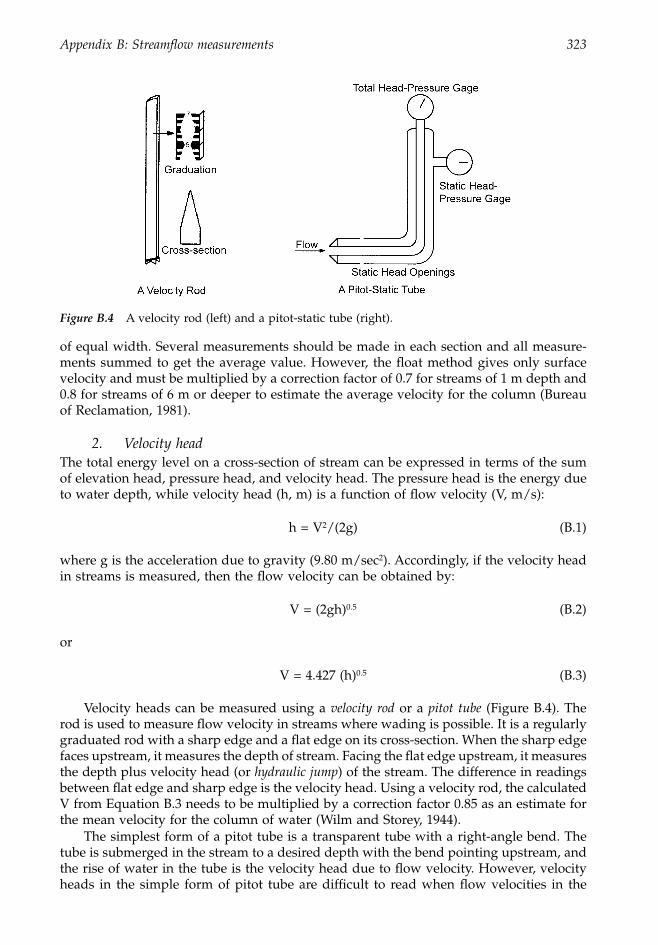
Appendix B: Streamflow measurements 323
of equal width. Several measurements should be made in each section and all measure-ments summed to get the average value. However, the float method gives only surfacevelocity and must be multiplied by a correction factor of 0.7 for streams of 1 m depth and0.8 for streams of 6 m or deeper to estimate the average velocity for the column (Bureauof Reclamation, 1981).
2. Velocity head
The total energy level on a cross-section of stream can be expressed in terms of the sumof elevation head, pressure head, and velocity head. The pressure head is the energy dueto water depth, while velocity head (h, m) is a function of flow velocity (V, m/s):
h = V
2
/(2g) (B.1)
where g is the acceleration due to gravity (9.80 m/sec
2
). Accordingly, if the velocity headin streams is measured, then the flow velocity can be obtained by:
V = (2gh)
0.5
(B.2)
or
V = 4.427 (h)
0.5
(B.3)
Velocity heads can be measured using a
velocity rod
or a
pitot tube
(Figure B.4). Therod is used to measure flow velocity in streams where wading is possible. It is a regularlygraduated rod with a sharp edge and a flat edge on its cross-section. When the sharp edgefaces upstream, it measures the depth of stream. Facing the flat edge upstream, it measuresthe depth plus velocity head (or
hydraulic jump
) of the stream. The difference in readingsbetween flat edge and sharp edge is the velocity head. Using a velocity rod, the calculatedV from Equation B.3 needs to be multiplied by a correction factor 0.85 as an estimate forthe mean velocity for the column of water (Wilm and Storey, 1944).
The simplest form of a pitot tube is a transparent tube with a right-angle bend. Thetube is submerged in the stream to a desired depth with the bend pointing upstream, andthe rise of water in the tube is the velocity head due to flow velocity. However, velocityheads in the simple form of pitot tube are difficult to read when flow velocities in the
Figure B.4
A velocity rod (left) and a pitot-static tube (right).
1363_ AppB_fm Page 323 Wednesday, December 4, 2002 7:47 AM
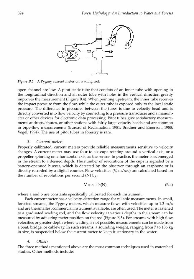
324 Forest Hydrology: An Introduction to Water and Forests
open channel are low. A pitot-static tube that consists of an inner tube with opening inthe longitudinal direction and an outer tube with holes in the vertical direction greatlyimproves the measurement (Figure B.4). When pointing upstream, the inner tube receivesthe impact pressure from the flow, while the outer tube is exposed only to the local staticpressure. The difference in pressures between the tubes is due to velocity head and isdirectly converted into flow velocity by connecting to a pressure transducer and a manom-eter or other devices for electronic data processing. Pitot tubes give satisfactory measure-ments at drops, chutes, or other stations with fairly large velocity heads and are commonin pipe-flow measurements (Bureau of Reclamation, 1981; Bradner and Emerson, 1988;Vogel, 1994). The use of pitot tubes in forestry is rare.
3. Current meters
Properly calibrated, current meters provide reliable measurements sensitive to velocitychanges. A current meter may use four to six cups rotating around a vertical axis, or apropeller spinning on a horizontal axis, as the sensor. In practice, the meter is submergedin the stream to a desired depth. The number of revolutions of the cups is signaled by abattery-operated buzzer, which is detected by the observer through an earphone or isdirectly recorded by a digital counter. Flow velocities (V, m/sec) are calculated based onthe number of revolutions per second (N) by:
V = a + b(N) (B.4)
where a and b are constants specifically calibrated for each instrument.Each current meter has a velocity-detection range for reliable measurements. In small,
forested streams, the Pygmy meters, which measure flows with velocities up to 1.3 m/sand are the smallest commercial instrument available, are often used. The meter is fastenedto a graduated wading rod, and the flow velocity at various depths in the stream can bemeasured by adjusting meter position on the rod (Figure B.5). For streams with high flowvelocities or greater depth where wading is not possible, measurements can be made froma boat, bridge, or cableway. In such streams, a sounding weight, ranging from 7 to 136 kgin size, is suspended below the current meter to keep it stationary in the water.
4. Others
The three methods mentioned above are the most common techniques used in watershedstudies. Other methods include:
Figure B.5
A Pygmy current meter on wading rod.
1363_ AppB_fm Page 324 Wednesday, December 4, 2002 7:47 AM
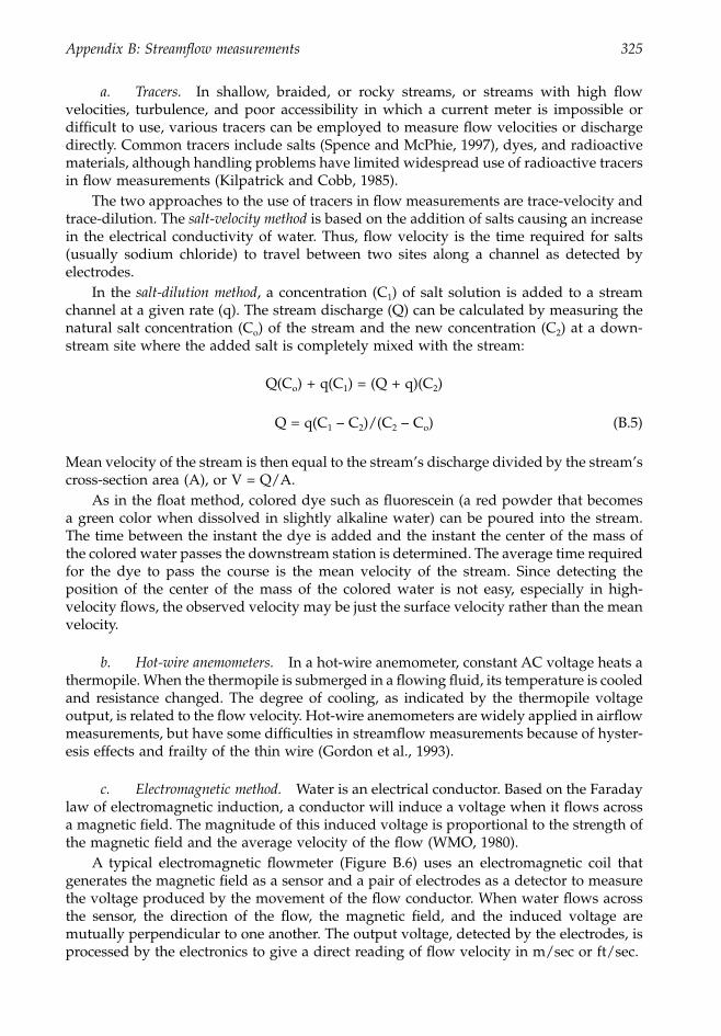
Appendix B: Streamflow measurements 325
a. Tracers.
In shallow, braided, or rocky streams, or streams with high flowvelocities, turbulence, and poor accessibility in which a current meter is impossible ordifficult to use, various tracers can be employed to measure flow velocities or dischargedirectly. Common tracers include salts (Spence and McPhie, 1997), dyes, and radioactivematerials, although handling problems have limited widespread use of radioactive tracersin flow measurements (Kilpatrick and Cobb, 1985).
The two approaches to the use of tracers in flow measurements are trace-velocity andtrace-dilution. The
salt-velocity method
is based on the addition of salts causing an increasein the electrical conductivity of water. Thus, flow velocity is the time required for salts(usually sodium chloride) to travel between two sites along a channel as detected byelectrodes.
In the
salt-dilution method
, a concentration (C
1
) of salt solution is added to a streamchannel at a given rate (q). The stream discharge (Q) can be calculated by measuring thenatural salt concentration (C
o
) of the stream and the new concentration (C
2
) at a down-stream site where the added salt is completely mixed with the stream:
Q(C
o
) + q(C
1
) = (Q + q)(C
2
)
Q = q(C
1
– C
2
)/(C
2
– C
o
) (B.5)
Mean velocity of the stream is then equal to the stream’s discharge divided by the stream’scross-section area (A), or V = Q/A.
As in the float method, colored dye such as fluorescein (a red powder that becomesa green color when dissolved in slightly alkaline water) can be poured into the stream.The time between the instant the dye is added and the instant the center of the mass ofthe colored water passes the downstream station is determined. The average time requiredfor the dye to pass the course is the mean velocity of the stream. Since detecting theposition of the center of the mass of the colored water is not easy, especially in high-velocity flows, the observed velocity may be just the surface velocity rather than the meanvelocity.
b. Hot-wire anemometers.
In a hot-wire anemometer, constant AC voltage heats athermopile. When the thermopile is submerged in a flowing fluid, its temperature is cooledand resistance changed. The degree of cooling, as indicated by the thermopile voltageoutput, is related to the flow velocity. Hot-wire anemometers are widely applied in airflowmeasurements, but have some difficulties in streamflow measurements because of hyster-esis effects and frailty of the thin wire (Gordon et al., 1993).
c. Electromagnetic method.
Water is an electrical conductor. Based on the Faradaylaw of electromagnetic induction, a conductor will induce a voltage when it flows acrossa magnetic field. The magnitude of this induced voltage is proportional to the strength ofthe magnetic field and the average velocity of the flow (WMO, 1980).
A typical electromagnetic flowmeter (Figure B.6) uses an electromagnetic coil thatgenerates the magnetic field as a sensor and a pair of electrodes as a detector to measurethe voltage produced by the movement of the flow conductor. When water flows acrossthe sensor, the direction of the flow, the magnetic field, and the induced voltage aremutually perpendicular to one another. The output voltage, detected by the electrodes, isprocessed by the electronics to give a direct reading of flow velocity in m/sec or ft/sec.
1363_ AppB_fm Page 325 Wednesday, December 4, 2002 7:47 AM
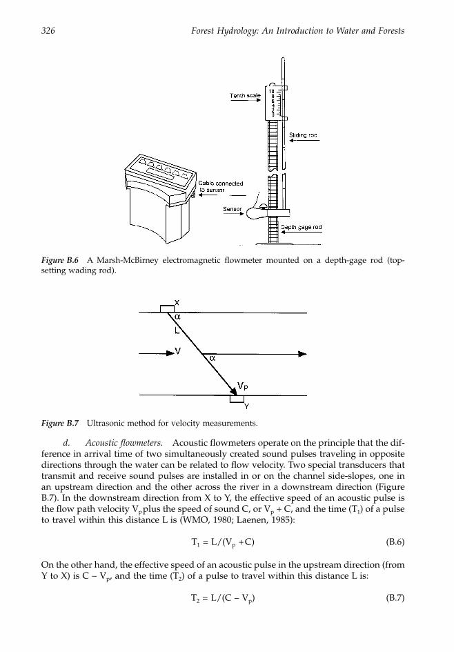
326 Forest Hydrology: An Introduction to Water and Forests
d. Acoustic flowmeters.
Acoustic flowmeters operate on the principle that the dif-ference in arrival time of two simultaneously created sound pulses traveling in oppositedirections through the water can be related to flow velocity. Two special transducers thattransmit and receive sound pulses are installed in or on the channel side-slopes, one inan upstream direction and the other across the river in a downstream direction (FigureB.7). In the downstream direction from X to Y, the effective speed of an acoustic pulse isthe flow path velocity V
p
plus the speed of sound C, or V
p
+ C, and the time (T
1
) of a pulseto travel within this distance L is (WMO, 1980; Laenen, 1985):
T
1
= L/(V
p
+
C) (B.6)
On the other hand, the effective speed of an acoustic pulse in the upstream direction (fromY to X) is C
-
V
p
, and the time (T
2
) of a pulse to travel within this distance L is:
T
2
= L/(C – V
p
) (B.7)
Figure B.6
A Marsh-McBirney electromagnetic flowmeter mounted on a depth-gage rod (top-setting wading rod).
Figure B.7
Ultrasonic method for velocity measurements.
1363_ AppB_fm Page 326 Wednesday, December 4, 2002 7:47 AM
Appendix B: Streamflow measurements 327
Thus, if the difference in transit time of the two simultaneously created pulses is known, or:
D
T = T
1
– T
2
= L/(C + V
p
) – L/(C – V
p
)
= 2L V
p
/(C
2
– V
p2
) (B.8)
Since C
2
is much greater than V
p2
, Equation B.8 can be simplified as:
D
T = (2LV
p2
)/C
2
(B.9)
or
V
p
=
D
TC
2
/(2L) (B.10)
The average flow velocity (V) at a given depth can be corrected by the inclined angle ofthe path line (
a
):
V = V
p
/(cos
a
) (B.11)
e. Acoustic Doppler current profiler.
The acoustic Doppler current profiler (ADCP)system is a modern technique developed by the U.S. Geological Survey to monitor hori-zontal and vertical water velocities at 1 m vertical intervals from a moving vessel. TheADCP transmits acoustic pulses into the water column. Part of the transmitted acousticenergy is reflected back toward the transducers by particulate matter in the water that isassumed to move with the water. The Doppler effect causes the frequency of these reflectedsignals to shift, and the magnitude of the frequency shift is a function of the speed of theparticulate matter along the acoustic beam. The frequency shifts are then converted intowater speeds by the computer software and hardware of the ADCP system. The systemis designed to overcome the difficulty, time consumption, and dangers associated withdischarge measurements in large rivers and estuaries (Simpson and Oltmann, 1993).
Note that the Doppler effect, named after the Austrian physicist Christian J. Doppler(1803–1853), describes our experience of the relative motion between the source and theobserver. When the source and observer are moving toward each other, the frequencyheard by the observer is higher than the frequency of the source. On the other hand, whenthey are moving away from each other, the frequency heard by the observer is lower thanthe frequency of the source. Some of the common applications of the Doppler effect includethe measurements of rainfall intensity, ocean waves and currents, flow velocity, andautomobile speed.
III. Discharge
A. Volumetric and gravimetric methods
In volumetric and gravimetric methods, the entire flow in a stream is collected in acontainer over a given time period. Sometimes it is necessary to build an artificial controlso that all the flows can be diverted into a calibrated container of known volume or weight.Discharge (Q, m
3
or l/sec) is calculated by the time (T, sec) required to fill a known volume(
v
, m
3
or l) of flow read directly from the container or calculated indirectly by placing thecontainer on a weighing scale:
1363_ AppB_fm Page 327 Wednesday, December 4, 2002 7:47 AM
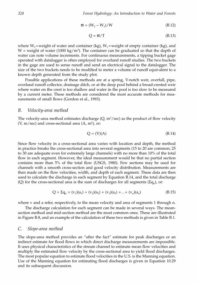
328 Forest Hydrology: An Introduction to Water and Forests
v
= (W
2
– W
1
)/W (B.12)
Q =
v
/T (B.13)
where W
2
=
weight of water and container (kg), W
1
=
weight of empty container (kg), andW = weight of water (1000 kg/m
3
). The container can be graduated so that the depth ofwater can note volume increments. For continuous measurements, a tipping bucket gageoperated with datalogger is often employed for overland runoff studies. The two bucketsin the gage are used to sense runoff and send an electrical signal to the datalogger. Thesize of the two buckets needs to be modified to meter a volume of runoff equivalent to aknown depth generated from the study plot.
Possible applications of these methods are at a spring, V-notch weir, overfall, pipe,overland runoff collector, drainage ditch, or at the deep pool behind a broad-crested weirwhere water on the crest is too shallow and water in the pool is too slow to be measuredby a current meter. These methods are considered the most accurate methods for mea-surements of small flows (Gordon et al., 1993).
B. Velocity-area method
The velocity-area method estimates discharge (Q, m
3
/sec) as the product of flow velocity(V, m/sec) and cross-sectional area (A, m
2
), or:
Q = (V)(A) (B.14)
Since flow velocity in a cross-sectional area varies with location and depth, the methodin practice breaks the cross-sectional area into several segments (15 to 20 are common; 25to 30 are adequate even for extremely large channels) with no more than 10% of the totalflow in each segment. However, the ideal measurement would be that no partial sectioncontains more than 5% of the total flow (USGS, 1980). Few sections may be used forchannels with a smooth cross-section and good velocity distribution. Measurements arethen made on the flow velocities, width, and depth of each segment. These data are thenused to calculate the discharge in each segment by Equation B.14, and the total discharge(Q) for the cross-sectional area is the sum of discharges for all segments (
S
q
n
), or:
Q =
S
q
n
= (v
1
)(a
1
) + (v
2
)(a
2
) + (v
3
)(a
3
) +…+ (v
n
)(a
n
) (B.15)
where v and a refer, respectively, to the mean velocity and area of segments 1 through n.The discharge calculation for each segment can be made in several ways. The mean-
section method and mid-section method are the most common ones. These are illustratedin Figure B.8, and an example of the calculation of these two methods is given in Table B.1.
C. Slope-area method
The slope-area method provides an “after the fact” estimate for peak discharges or anindirect estimate for flood flows in which direct discharge measurements are impossible.It uses physical characteristics of the stream channel to estimate mean flow velocities andmultiply the estimated flow velocity by the cross-sectional area to yield flood discharges.The most popular equation to estimate flood velocities in the U.S. is the Manning equation.Use of the Manning equation for estimating flood discharges is given in Equation 10.29and its subsequent discussion.
1363_ AppB_fm Page 328 Wednesday, December 4, 2002 7:47 AM
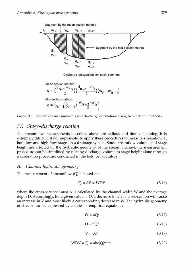
Appendix B: Streamflow measurements 329
IV. Stage–discharge relation
The streamflow measurements described above are tedious and time consuming. It isextremely difficult, if not impossible, to apply these procedures to measure streamflow atboth low and high flow stages in a drainage system. Since streamflow volume and stageheight are affected by the hydraulic geometry of the stream channel, the measurementprocedure can be simplified by relating discharge volume to stage height alone througha calibration procedure conducted in the field or laboratory.
A. Channel hydraulic geometry
The measurement of streamflow (Q) is based on:
Q = AV = WDV (B.16)
where the cross-sectional area A is calculated by the channel width W and the averagedepth D. Accordingly, for a given value of Q, a decrease in D at a cross-section will causean increase in V and most likely a corresponding decrease in W. The hydraulic geometryof streams can be expressed by a series of empirical equations:
W = aQ
x
(B.17)
D = bQ
y
(B.18)
V = cQ
z
(B.19)
WDV = Q = abc(Q)
(x+y+z)
(B.20)
Figure B.8
Streamflow measurements and discharge calculations using two different methods.
1363_ AppB_fm Page 329 Wednesday, December 4, 2002 7:47 AM
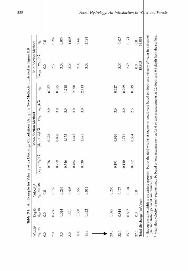
330 Forest Hydrology: An Introduction to Water and Forests
Tabl
e B
.1
An
Exa
mpl
e fo
r V
eloc
ity-
Are
a D
isch
arge
Cal
cula
tion
s U
sing
the
Tw
o M
etho
ds
Illu
stra
ted
in F
igur
e B
.8
Wid
th
a
Dep
thV
eloc
ity
b
Mea
n-Se
ctio
n M
etho
d
Mid
-Sec
tion
Met
hod
w
n
, md
n
, mv
n
, m/
sec
(v
n
-
1
+ v
n
)/2
(d
n
-
1
+ d
n
)/2
(w
n
-
wn-
1)/
2q n
(wn+
1 -
wn-
1)/
2q n
0.0
0.0
0.0
0.0
0.0
0.07
60.
378
2.0
0.05
72.
00.
756
0.15
22.
500.
287
0.21
90.
890
3.0
0.58
55.
01.
024
0.28
63.
000.
879
0.34
61.
173
3.0
1.21
88.
01.
321
0.40
53.
001.
605
0.48
41.
445
3.0
2.09
811
.01.
568
0.56
33.
002.
648
0.53
81.
495
3.0
2.41
314
.01.
422
0.51
23.
002.
184
29.0
1.02
50.
206
0.19
10.
920
3.0
0.52
732
.00.
814
0.17
53.
000.
427
0.14
00.
711
3.0
0.29
935
.00.
607
0.10
42.
750.
174
0.05
20.
304
2.5
0.01
937
.50.
00.
00.
00.
0To
tal d
isch
arge
(m
3 /se
c)15
.805
16.0
54
aH
avin
g th
e sa
me
wid
th is
the
eas
iest
app
roac
h, b
ut in
the
fiel
d w
idth
s of
seg
men
ts w
ould
var
y ba
sed
on
dep
th a
nd v
eloc
ity
of w
ater
in a
cha
nnel
(Dr.
Don
Tur
ton,
per
sona
l com
mun
icat
ion)
.b
Mea
n fl
ow v
eloc
ity
of e
ach
segm
ent
may
be
base
d o
n on
e m
easu
rem
ent
at 0
.6 d
or
two
mea
sure
men
ts a
t 0.
2 d
epth
and
0.6
dep
th f
rom
the
sur
face
.
1363_ AppB_fm Page 330 Wednesday, December 4, 2002 7:47 AM
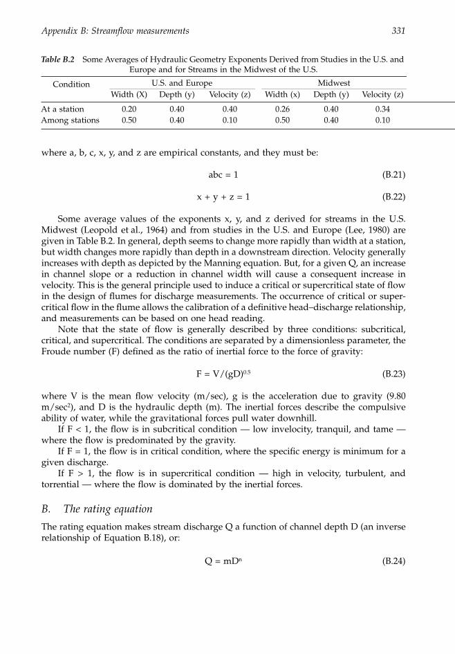
Appendix B: Streamflow measurements 331
where a, b, c, x, y, and z are empirical constants, and they must be:
abc = 1 (B.21)
x + y + z = 1 (B.22)
Some average values of the exponents x, y, and z derived for streams in the U.S.Midwest (Leopold et al., 1964) and from studies in the U.S. and Europe (Lee, 1980) aregiven in Table B.2. In general, depth seems to change more rapidly than width at a station,but width changes more rapidly than depth in a downstream direction. Velocity generallyincreases with depth as depicted by the Manning equation. But, for a given Q, an increasein channel slope or a reduction in channel width will cause a consequent increase invelocity. This is the general principle used to induce a critical or supercritical state of flowin the design of flumes for discharge measurements. The occurrence of critical or super-critical flow in the flume allows the calibration of a definitive head–discharge relationship,and measurements can be based on one head reading.
Note that the state of flow is generally described by three conditions: subcritical,critical, and supercritical. The conditions are separated by a dimensionless parameter, theFroude number (F) defined as the ratio of inertial force to the force of gravity:
F = V/(gD)0.5 (B.23)
where V is the mean flow velocity (m/sec), g is the acceleration due to gravity (9.80m/sec2), and D is the hydraulic depth (m). The inertial forces describe the compulsiveability of water, while the gravitational forces pull water downhill.
If F < 1, the flow is in subcritical condition — low invelocity, tranquil, and tame —where the flow is predominated by the gravity.
If F = 1, the flow is in critical condition, where the specific energy is minimum for agiven discharge.
If F > 1, the flow is in supercritical condition — high in velocity, turbulent, andtorrential — where the flow is dominated by the inertial forces.
B. The rating equation
The rating equation makes stream discharge Q a function of channel depth D (an inverserelationship of Equation B.18), or:
Q = mDn (B.24)
Table B.2 Some Averages of Hydraulic Geometry Exponents Derived from Studies in the U.S. and Europe and for Streams in the Midwest of the U.S.
Condition U.S. and Europe MidwestWidth (X) Depth (y) Velocity (z) Width (x) Depth (y) Velocity (z)
At a station 0.20 0.40 0.40 0.26 0.40 0.34Among stations 0.50 0.40 0.10 0.50 0.40 0.10
1363_ AppB_fm Page 331 Wednesday, December 4, 2002 7:47 AM
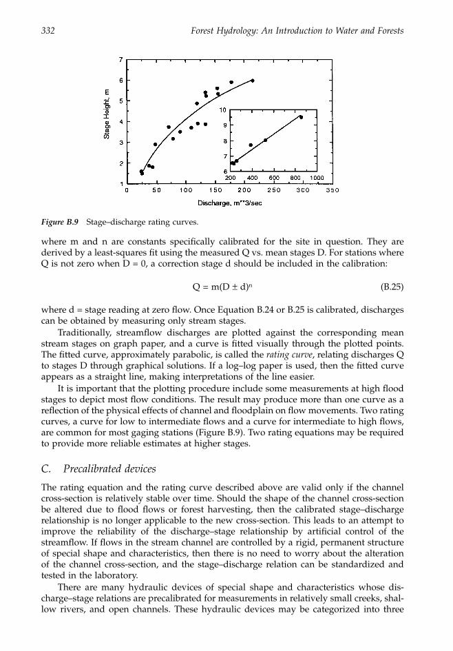
332 Forest Hydrology: An Introduction to Water and Forests
where m and n are constants specifically calibrated for the site in question. They arederived by a least-squares fit using the measured Q vs. mean stages D. For stations whereQ is not zero when D = 0, a correction stage d should be included in the calibration:
Q = m(D ± d)n (B.25)
where d = stage reading at zero flow. Once Equation B.24 or B.25 is calibrated, dischargescan be obtained by measuring only stream stages.
Traditionally, streamflow discharges are plotted against the corresponding meanstream stages on graph paper, and a curve is fitted visually through the plotted points.The fitted curve, approximately parabolic, is called the rating curve, relating discharges Qto stages D through graphical solutions. If a log–log paper is used, then the fitted curveappears as a straight line, making interpretations of the line easier.
It is important that the plotting procedure include some measurements at high floodstages to depict most flow conditions. The result may produce more than one curve as areflection of the physical effects of channel and floodplain on flow movements. Two ratingcurves, a curve for low to intermediate flows and a curve for intermediate to high flows,are common for most gaging stations (Figure B.9). Two rating equations may be requiredto provide more reliable estimates at higher stages.
C. Precalibrated devices
The rating equation and the rating curve described above are valid only if the channelcross-section is relatively stable over time. Should the shape of the channel cross-sectionbe altered due to flood flows or forest harvesting, then the calibrated stage–dischargerelationship is no longer applicable to the new cross-section. This leads to an attempt toimprove the reliability of the discharge–stage relationship by artificial control of thestreamflow. If flows in the stream channel are controlled by a rigid, permanent structureof special shape and characteristics, then there is no need to worry about the alterationof the channel cross-section, and the stage–discharge relation can be standardized andtested in the laboratory.
There are many hydraulic devices of special shape and characteristics whose dis-charge–stage relations are precalibrated for measurements in relatively small creeks, shal-low rivers, and open channels. These hydraulic devices may be categorized into three
Figure B.9 Stage–discharge rating curves.
1363_ AppB_fm Page 332 Wednesday, December 4, 2002 7:47 AM
Appendix B: Streamflow measurements 333
types: weirs, flumes, and orifices. Weirs and flumes are used in open channels, whileorifices are associated with submerged sluices, regulated or unregulated gates, and pipeflows. The use of weirs and flumes depends on stream size, flow range, channel gradient,and sediment load. When orifices are not submerged, they may act as a weir.
1. Weirs
a. Features. A weir is a dam built across an open channel for flow measurements.Weirs are barriers on the bottom of stream channels that cause the overflow of water toaccelerate. Components of a weir include:
1. A crest of specific shape, usually high above the bottom of the stream channel, forwater-head determination
2. A bulkhead to form a water pool behind the weir3. An approach section long enough to allow water approaching the weir with a
minimum velocity free from turbulence4. Two side walls to ensure that all overland and subsurface runoff passes through
the weir5. A stilling well, equipped with an electrical water-level recorder, installed a few feet
behind the weir6. An opening beneath the crest of the weir bulkhead to sluice accumulated sediment
The discharge rate of the channel is determined by measuring water head above theweir crest. The head can then be converted into discharge rate by a standard equationspecifically calibrated for the shape and size of the weir. Weirs are not suitable for instal-lations in channels with flat slopes or carrying excessive solid materials and sediment(Grant, 1992). Accordingly, openings beneath the crest are a mechanism to clean theaccumulation of sediment, and the crest must be kept free from fibers, stringy materials,and other articles. If installed properly, weirs are the most reliable structures for measuringwater in canals and ditches.
b. Types of weirs. Weirs can be classified in several ways. By the shapes of crest,they can be rectangular, triangular (V-notch), and trapezoidal (Cippoletti). By the contactof flows to the crest, they can be sharp-crested (thin-plate weirs) and broad-crested weirs.A sharp-crested weir has a vertical flat plate with a sharpened upper edge installed alongthe crest so that water does not contact any part of the weir structure downstream. Broad-crested weirs have a solid broad section of concrete or other material such that waterflows over the entire surface of the crest. Broad-crested weirs are not as popular as sharp-crested weirs, which can be rectangular, triangular, and trapezoidal, and are often existingstructures such as dams or levees. Discharges are obtained by a calibration procedure inthe field.
Classified by the crest length of the rectangular weir in respect to the channel cross-section, there are weirs without end contractions (suppressed weirs) and weirs with endcontractions (contracted weirs). A suppressed weir extends the weir’s crest length to thefull span of the channel, while a weir with its crest length less than the width of thechannel is said to have end contractions.
Classified by the downstream water level below the weir’s crest, weirs are referredto as free or critical and submerged or subcritical. The sheet of water passing the weircrest is called the nappe. When the water level downstream from the weir is low enoughto allow free air movement beneath the nappe, the underside of the nappe or water jet isexposed to the atmospheric pressure and the flow is referred to as free or critical. This
1363_ AppB_fm Page 333 Wednesday, December 4, 2002 7:47 AM
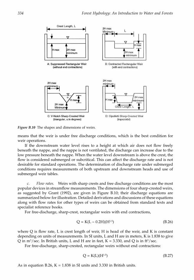
334 Forest Hydrology: An Introduction to Water and Forests
means that the weir is under free discharge conditions, which is the best condition forweir operations.
If the downstream water level rises to a height at which air does not flow freelybeneath the nappe, and the nappe is not ventilated, the discharge can increase due to thelow pressure beneath the nappe. When the water level downstream is above the crest, theflow is considered submerged or subcritical. This can affect the discharge rate and is notdesirable for standard operations. The determination of discharge rate under submergedconditions requires measurements of both upstream and downstream heads and use ofsubmerged weir tables.
c. Flow rates. Weirs with sharp crests and free discharge conditions are the mostpopular devices in streamflow measurements. The dimensions of four sharp-crested weirs,as suggested by Grant (1992), are given in Figure B.10; their discharge equations aresummarized below for illustration. Detailed derivations and discussions of these equationsalong with flow rates for other types of weirs can be obtained from standard texts andspecialist reference books.
For free-discharge, sharp-crest, rectangular weirs with end contractions,
Q = K(L – 0.2H)(H1.5) (B.26)
where Q is flow rate, L is crest length of weir, H is head of the weir, and K is constantdepending on units of measurements. In SI units, L and H are in meters, K is 1.838 to giveQ in m3/sec. In British units, L and H are in feet, K = 3.330, and Q is in ft3/sec.
For free-discharge, sharp-crested, rectangular weirs without end contractions:
Q = K(L)(H1.5) (B.27)
As in equation B.26, K = 1.838 in SI units and 3.330 in British units.
Figure B.10 The shapes and dimensions of weirs.
1363_ AppB_fm Page 334 Wednesday, December 4, 2002 7:47 AM
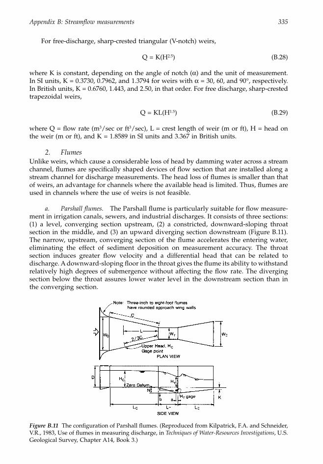
Appendix B: Streamflow measurements 335
For free-discharge, sharp-crested triangular (V-notch) weirs,
Q = K(H2.5) (B.28)
where K is constant, depending on the angle of notch (a) and the unit of measurement.In SI units, K = 0.3730, 0.7962, and 1.3794 for weirs with a = 30, 60, and 90∞, respectively.In British units, K = 0.6760, 1.443, and 2.50, in that order. For free discharge, sharp-crestedtrapezoidal weirs,
Q = KL(H1.5) (B.29)
where Q = flow rate (m3/sec or ft3/sec), L = crest length of weir (m or ft), H = head onthe weir (m or ft), and K = 1.8589 in SI units and 3.367 in British units.
2. FlumesUnlike weirs, which cause a considerable loss of head by damming water across a streamchannel, flumes are specifically shaped devices of flow section that are installed along astream channel for discharge measurements. The head loss of flumes is smaller than thatof weirs, an advantage for channels where the available head is limited. Thus, flumes areused in channels where the use of weirs is not feasible.
a. Parshall flumes. The Parshall flume is particularly suitable for flow measure-ment in irrigation canals, sewers, and industrial discharges. It consists of three sections:(1) a level, converging section upstream, (2) a constricted, downward-sloping throatsection in the middle, and (3) an upward diverging section downstream (Figure B.11).The narrow, upstream, converging section of the flume accelerates the entering water,eliminating the effect of sediment deposition on measurement accuracy. The throatsection induces greater flow velocity and a differential head that can be related todischarge. A downward-sloping floor in the throat gives the flume its ability to withstandrelatively high degrees of submergence without affecting the flow rate. The divergingsection below the throat assures lower water level in the downstream section than inthe converging section.
Figure B.11 The configuration of Parshall flumes. (Reproduced from Kilpatrick, F.A. and Schneider,V.R., 1983, Use of flumes in measuring discharge, in Techniques of Water-Resources Investigations, U.S.Geological Survey, Chapter A14, Book 3.)
1363_ AppB_fm Page 335 Wednesday, December 4, 2002 7:47 AM
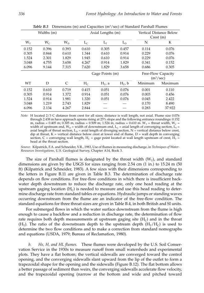
336 Forest Hydrology: An Introduction to Water and Forests
The size of Parshall flumes is designated by the throat width (WT), and standarddimensions are given by the USGS for sizes ranging from 2.54 cm (1 in.) to 15.24 m (50ft) (Kilpatrick and Schneider, 1983). A few sizes with their dimensions corresponding tothe letters in Figure B.11 are given in Table B.3. The determination of discharge ratedepends on flow conditions. For free-flow conditions in which there is insufficient back-water depth downstream to reduce the discharge rate, only one head reading at theupstream gaging location (HC) is needed to measure and use this head reading to deter-mine discharge rate from standard tables or equations. Hydraulic jumps or standing wavesoccurring downstream from the flume are an indicator of the free-flow condition. Thestandard equations for three throat sizes are given in Table B.4, in both British and SI units.
For submerged flows in which the water surface downstream from the flume is highenough to cause a backflow and a reduction in discharge rate, the determination of flowrate requires both depth measurements at upstream gaging site (HC) and in the throat(HT). The ratio of the downstream depth to the upstream depth (HT/HC) is used todetermine the two flow conditions and to make a correction from standard nomographsand equations (USDA, 1979; Bureau of Reclamation, 1980).
b. Hs, H, and HL flumes. These flumes were developed by the U.S. Soil Conser-vation Service in the 1930s to measure runoff from small watersheds and experimentalplots. They have a flat bottom; the vertical sidewalls are converged toward the controlopening, and the converging sidewalls slant upward from the lip of the outlet to form atrapezoidal shape for the opening and the sidewalls (Figure B.12). The flat bottom allowsa better passage of sediment than weirs, the converging sidewalls accelerate flow velocity,and the trapezoidal opening (narrow at the bottom and wide and pitched toward
Table B.3 Dimensions (m) and Capacities (m3/sec) of Standard Parshall Flumes
Widths (m) Axial Lengths (m) Vertical Distance Below Crest (m)
WT WC WD LC LT LD N K
0.152 0.396 0.393 0.610 0.305 0.457 0.114 0.0760.305 0.844 0.610 1.344 0.610 0.914 0.229 0.0761.524 2.301 1.829 1.945 0.610 0.914 0.229 0.0763.048 4.755 3.658 4.267 0.914 1.829 0.341 0.1526.096 9.144 7.315 7.620 1.829 3.658 0.686 0.305
Gage Points (m) Free-Flow Capacity(m3/sec)
WT D C HC HT, a HT, b Minimum Maximum
0.152 0.610 0.719 0.415 0.051 0.076 0.001 0.1100.305 0.914 1.372 0.914 0.051 0.076 0.003 0.4561.524 0.914 1.981 1.320 0.051 0.076 0.045 2.4223.048 1.219 2.743 1.829 — — 0.170 8.4906.096 2.134 4.267 2.844 — — 0.283 37.922
Note: H located 2/3 C distance from crest for all sizes; distance is wall length, not axial. Flume size 0.076through 2.438 m have approach aprons rising at 25% slope and the following entrance roundings: 0.152m, radius = 0.405 m; 0.305 m, radius = 0.509 m; 1.524 m, radius = 0.610 m. WT = throat width, WC =width of upstream end, WD = width of downstream end, LC = axial length of converging section, LT =axial length of throat section, LD = axial length of diverging section, N = vertical distance below crest,dip at throat, K = vertical distance below crest at lower end of flume, D = wall depth in convergingsection, C = converging wall length, HC = gage point located at wall length upstream of crest, HT =head at the throat section.
Source: Kilpatrick, F.A. and Schneider, V.R., 1983, Use of flumes in measuring discharge, in Techniques of Water-Resources Investigations, U.S. Geological Survey, Chapter A14, Book 3.
1363_ AppB_fm Page 336 Wednesday, December 4, 2002 7:47 AM
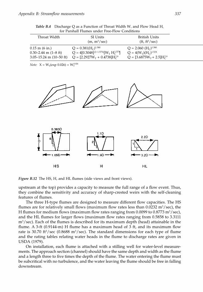
Appendix B: Streamflow measurements 337
upstream at the top) provides a capacity to measure the full range of a flow event. Thus,they combine the sensitivity and accuracy of sharp-crested weirs with the self-cleaningfeatures of flumes.
The three H-type flumes are designed to measure different flow capacities. The HSflumes are for relatively small flows (maximum flow rates less than 0.0232 m3/sec), theH flumes for medium flows (maximum flow rates ranging from 0.0099 to 0.8773 m3/sec),and the HL flumes for larger flows (maximum flow rates ranging from 0.5858 to 3.3111m3/sec). Each of the flumes is described for its maximum depth (head) attainable in theflume. A 3-ft (0.9144-m) H flume has a maximum head of 3 ft, and its maximum flowrate is 30.70 ft3/sec (0.8688 m3/sec). The standard dimensions for each type of flumeand the rating tables relating water heads in the flume to discharge rates are given inUSDA (1979).
On installation, each flume is attached with a stilling well for water-level measure-ments. The approach section (channel) should have the same depth and width as the flumeand a length three to five times the depth of the flume. The water entering the flume mustbe subcritical with no turbulence, and the water leaving the flume should be free in fallingdownstream.
Table B.4 Discharge Q as a Function of Throat Width WT and Flow Head HC for Parshall Flumes under Free-Flow Conditions
Throat Width SI Units(m, m3/sec)
British Units(ft, ft3/sec)
0.15 m (6 in.) Q = 0.381(HC)1.580 Q = 2.060 (HC)1.580
0.30–2.44 m (1–8 ft) Q = 4[0.3048](2-1.57X)[WT HC1.57X] Q = 4(WT)(HC)1.52X
3.05–15.24 m (10–50 ft) Q = [2.2927WT + 0.4738]HC1.6 Q = [3.6875WT + 2.5]HC
1.6
Note: X = WT(exp 0.026) = WT0.026
Figure B.12 The HS, H, and HL flumes (side views and front views).
1363_ AppB_fm Page 337 Wednesday, December 4, 2002 7:47 AM
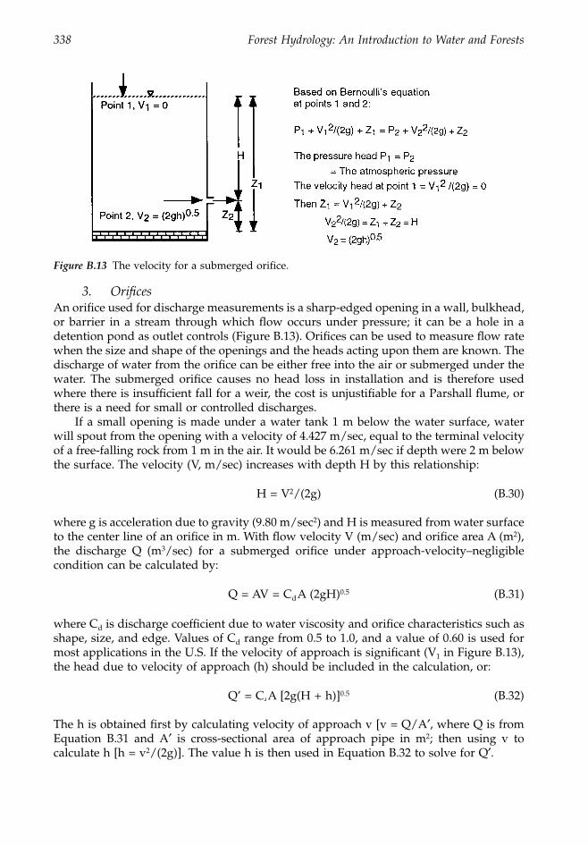
338 Forest Hydrology: An Introduction to Water and Forests
3. OrificesAn orifice used for discharge measurements is a sharp-edged opening in a wall, bulkhead,or barrier in a stream through which flow occurs under pressure; it can be a hole in adetention pond as outlet controls (Figure B.13). Orifices can be used to measure flow ratewhen the size and shape of the openings and the heads acting upon them are known. Thedischarge of water from the orifice can be either free into the air or submerged under thewater. The submerged orifice causes no head loss in installation and is therefore usedwhere there is insufficient fall for a weir, the cost is unjustifiable for a Parshall flume, orthere is a need for small or controlled discharges.
If a small opening is made under a water tank 1 m below the water surface, waterwill spout from the opening with a velocity of 4.427 m/sec, equal to the terminal velocityof a free-falling rock from 1 m in the air. It would be 6.261 m/sec if depth were 2 m belowthe surface. The velocity (V, m/sec) increases with depth H by this relationship:
H = V2/(2g) (B.30)
where g is acceleration due to gravity (9.80 m/sec2) and H is measured from water surfaceto the center line of an orifice in m. With flow velocity V (m/sec) and orifice area A (m2),the discharge Q (m3/sec) for a submerged orifice under approach-velocity–negligiblecondition can be calculated by:
Q = AV = Cd A (2gH)0.5 (B.31)
where Cd is discharge coefficient due to water viscosity and orifice characteristics such asshape, size, and edge. Values of Cd range from 0.5 to 1.0, and a value of 0.60 is used formost applications in the U.S. If the velocity of approach is significant (V1 in Figure B.13),the head due to velocity of approach (h) should be included in the calculation, or:
Q’ = Cd A [2g(H + h)]0.5 (B.32)
The h is obtained first by calculating velocity of approach v [v = Q/A¢, where Q is fromEquation B.31 and A¢ is cross-sectional area of approach pipe in m2; then using v tocalculate h [h = v2/(2g)]. The value h is then used in Equation B.32 to solve for Q¢.
Figure B.13 The velocity for a submerged orifice.
1363_ AppB_fm Page 338 Wednesday, December 4, 2002 7:47 AM
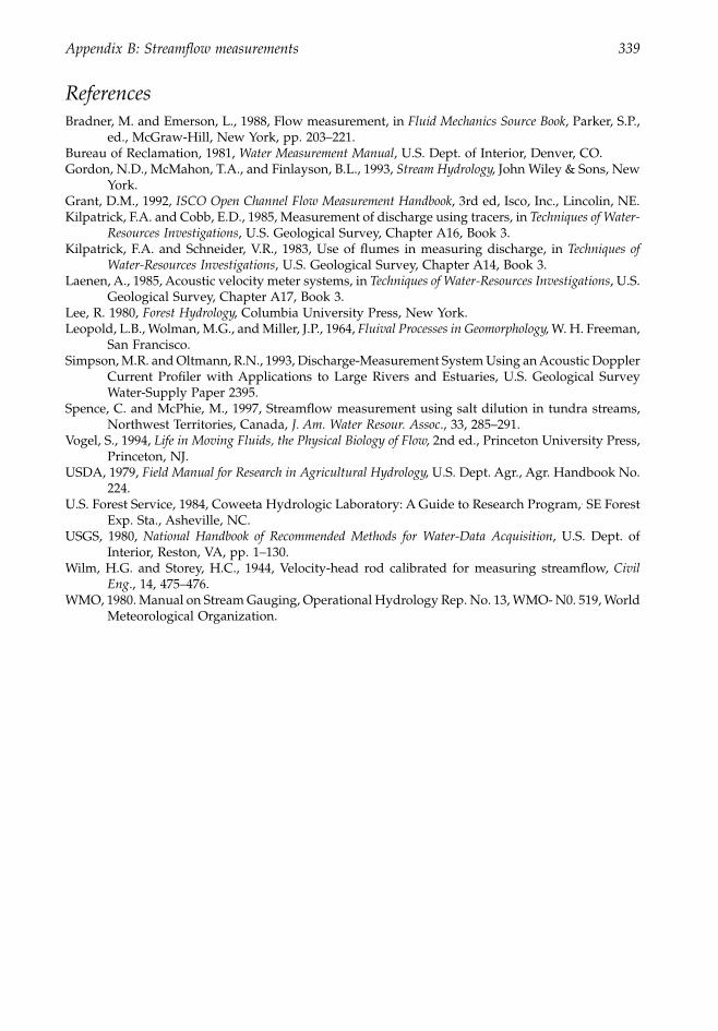
Appendix B: Streamflow measurements 339
ReferencesBradner, M. and Emerson, L., 1988, Flow measurement, in Fluid Mechanics Source Book, Parker, S.P.,
ed., McGraw-Hill, New York, pp. 203–221.Bureau of Reclamation, 1981, Water Measurement Manual, U.S. Dept. of Interior, Denver, CO.Gordon, N.D., McMahon, T.A., and Finlayson, B.L., 1993, Stream Hydrology, John Wiley & Sons, New
York.Grant, D.M., 1992, ISCO Open Channel Flow Measurement Handbook, 3rd ed, Isco, Inc., Lincolin, NE.Kilpatrick, F.A. and Cobb, E.D., 1985, Measurement of discharge using tracers, in Techniques of Water-
Resources Investigations, U.S. Geological Survey, Chapter A16, Book 3.Kilpatrick, F.A. and Schneider, V.R., 1983, Use of flumes in measuring discharge, in Techniques of
Water-Resources Investigations, U.S. Geological Survey, Chapter A14, Book 3.Laenen, A., 1985, Acoustic velocity meter systems, in Techniques of Water-Resources Investigations, U.S.
Geological Survey, Chapter A17, Book 3.Lee, R. 1980, Forest Hydrology, Columbia University Press, New York.Leopold, L.B., Wolman, M.G., and Miller, J.P., 1964, Fluival Processes in Geomorphology, W. H. Freeman,
San Francisco.Simpson, M.R. and Oltmann, R.N., 1993, Discharge-Measurement System Using an Acoustic Doppler
Current Profiler with Applications to Large Rivers and Estuaries, U.S. Geological SurveyWater-Supply Paper 2395.
Spence, C. and McPhie, M., 1997, Streamflow measurement using salt dilution in tundra streams,Northwest Territories, Canada, J. Am. Water Resour. Assoc., 33, 285–291.
Vogel, S., 1994, Life in Moving Fluids, the Physical Biology of Flow, 2nd ed., Princeton University Press,Princeton, NJ.
USDA, 1979, Field Manual for Research in Agricultural Hydrology, U.S. Dept. Agr., Agr. Handbook No.224.
U.S. Forest Service, 1984, Coweeta Hydrologic Laboratory: A Guide to Research Program,. SE ForestExp. Sta., Asheville, NC.
USGS, 1980, National Handbook of Recommended Methods for Water-Data Acquisition, U.S. Dept. ofInterior, Reston, VA, pp. 1–130.
Wilm, H.G. and Storey, H.C., 1944, Velocity-head rod calibrated for measuring streamflow, CivilEng., 14, 475–476.
WMO, 1980. Manual on Stream Gauging, Operational Hydrology Rep. No. 13, WMO- N0. 519, WorldMeteorological Organization.
1363_ AppB_fm Page 339 Wednesday, December 4, 2002 7:47 AM

1363_ AppB_fm Page 340 Wednesday, December 4, 2002 7:47 AM
341
Appendix C
Measurements of stream sediment
Contents
I. Suspended sediment.......................................................................................................342A. Sediment variation..................................................................................................342B. Sampling...................................................................................................................342
1. Site selection ......................................................................................................3422. Number of verticals..........................................................................................3433. Sampling frequency..........................................................................................3434. Types of samples...............................................................................................3445. Procedures for depth-integrated samplers ...................................................344
a. The EDI method..........................................................................................345b. The ETR method .........................................................................................346
6. Procedures for point-integrating samplers...................................................346C. Measuring devices ..................................................................................................346
1. Hand-operated samplers .................................................................................3462. Automatic samplers .........................................................................................348
a. Mechanical samplers ..................................................................................348b. Electrical pumping samplers ....................................................................349c. Optical turbidity systems ..........................................................................349d. Acoustic Doppler current profiler (ADCP) ............................................350e. Radioactive turbiometric gages ................................................................351
D. Calculations .............................................................................................................3511. Suspended-sediment load for a cross section..............................................3512. Mean suspended-sediment concentration....................................................3513. Suspended-sediment load for a runoff event ..............................................352
II. Bedload .............................................................................................................................352A. Bedload variation....................................................................................................352B. Sampling...................................................................................................................353C. Measuring devices ..................................................................................................355
1. Bedload samplers..............................................................................................335a. Basket-type samplers..................................................................................355b. Tray samplers ..............................................................................................355c. Pressure-difference samplers ....................................................................355d. Sediment traps.............................................................................................355
2. Tracers.................................................................................................................3563. Acoustic and ultrasonic measurement..........................................................357
D. Calculations .............................................................................................................357References .....................................................................................................................................358
1363_ AppC_fm Page 341 Wednesday, December 4, 2002 7:47 AM
342 Forest Hydrology: An Introduction to Water and Forests
Stream sediment, or fluvial sediment, refers to the fragmental material and particles thatare retained and transported in stream channels. These materials are derived primarilyfrom the physical and chemical disintegration of rocks and delivery to stream channelsvia various erosion phases including raindrop splash, interrill, rill, gullies, channel, andmass movement. Sediment information is required for: (1) evaluation of land-use man-agement, (2) the design of hydraulic structures, (3) water-quality management, (4) waterutilization, and (5) aquatic-life management.
Sediments in streams appear as washload, suspended load, and bedload. Washloadand suspended load are those fine sediments that are transported in streams with no directcontact with the streambed for an appreciable length of time, while bedload consists ofthose particles rolling and bouncing along the streambed. In measurement, sediments insuspended load and washload are separated from bedload.
I. Suspended sediment
Suspended sediments are supported by the fluid and carried along above the layer oflaminar flow. They have settling velocities less than the buoyant velocity of the flow andstay in suspension in the water for an appreciable length of time. Suspended sedimentsin the stream are measured in terms of sediment concentration in mg/l (mass per unitvolume of streamflow), based on water samples collected in the field and gravimetricallydetermined in the laboratory. The sediment concentration is then weighted by the flowrates measured simultaneously to obtain sediment yield (or discharge) in t/day (or otherunits in mass per unit time). Finally, the sediment yield in mass/time is divided by thewatershed area to give the result in mass/time/area for comparisons with other studies.
A. Sediment variation
The concentration of suspended sediment varies with depth, velocity, turbulence, particlesize and shape, channel geometry, physical and chemical properties of water, watershedsize and topographic characteristics, climatic conditions, and time. The variation is greaterin small watersheds than in large watersheds because of small watersheds’ sensitivity tostorm characteristics. For a given cross section, the greatest concentration is near the bedand decreases to minimum at the surface. It is more concentrated in the segments wherevelocity is high and depth is low. During high flows, total suspended sediment can begreater than that in low flows by a factor of more than 1000 (Bonta, 2000). Consequently,the majority of annual sediment yield can be attributable to only a few major storms. A200 km
2
watershed in Wisconsin (U.S.), cited by Garde and Ranga Raju (1985), generated90% of the total sediment load of a 15-month period in 10 days, or 2.2% of the time.Likewise, a 7-year study on the River Creedy in Devon, U.K. showed that 80% of thesediment load was carried in 3% of the time (Walling and Webb, 1981).
B. Sampling
1. Site selection
Sampling sites are selected with consideration of the data needs and the nature of theflow and channel conditions. Because streamflow discharge is also required in mostsediment measurements, existing stream-gaging stations are logical sites for samplingsuspended sediments. At such stations, samples should be taken upstream of still ponds(Gordon et al., 1992). If no suitable gaging station already exists, then the sampling site
1363_ AppC_fm Page 342 Wednesday, December 4, 2002 7:47 AM
Appendix C: Measurements of stream sediment 343
should be located in the middle section of a straight reach of length at least four timesthe width of the channel, but no less than 150 m (Singhal et al., 1981). In mountainousregions where straight reaches are difficult to find, a length of 50 m should be acceptable.
Flow conditions at sites such as those downstream or upstream from the confluenceof two streams can be disturbed by unusual water-surface slopes, lateral flows, back flows,and mixing effects. These conditions will likewise affect the normal movement of sedimentand may require additional sediment measurements. Also, sites should not be adjacent tohydraulic structures. A measuring section at a bend should be avoided because of unevendistribution of stream energy. Likewise, sites with unstable cross sections, such as activebank erosion, silting, and scouring, should not be used for measurements. Because moresamples are required during periods of high flows, it is imperative that sites be accessibleduring times of flooding.
If samples are required for the assessment of land-treatment effects, then the samplingsites are obvious. They should be close to the treatments, both upstream and downstreamlocations. Locating too far from the treatment sites can cause the dilution effect of stream-flow to be significant. Changes in hydraulic and channel conditions between sites increasewith distance.
2. Number of verticals
The number of verticals required in sampling suspended sediment along a stream’s crosssection depend on the type of information needed, the degree of accuracy required, andthe physical aspects of the river. It may be determined based on statistical approaches orfield experience. The number has ranged from a single vertical for small streams to morethan 15 verticals for streams with great sediment variations. If only the smaller fractionssuch as silts and clays are of concern, then one grab sample taken near the water surfacein the center of the stream is considered sufficient (Gordon et al., 1992). Sampling at asingle vertical is also adequate if a stream’s cross section is stable and its lateral suspended-sediment distribution is rather uniform. If the distribution of sediment concentration orparticle size across the stream is important, then samples are needed at several verticals.
For sand-bed streams, the bed configuration can vary significantly across and alongthe stream, as can the sediment concentration. Such streams may require more samplingverticals to estimate the sediment concentration of the cross section. Samplings at 6 to 12verticals are usually sufficient to produce a reliable estimate of discharge-weighted sus-pended sediment for most small streams (USDA, 1979).
3. Sampling frequency
Suspended-sediment concentration in a given stream is highly variable with time. It isoften much higher during floods, on the increasing discharge during a flood (the risinglimb of the hydrograph), and for storms preceded by a long, dry period (MacDonald et al.,1991), but is lower for runoff generated from snow storms than from rain storms. Sus-pended-sediment sampling is therefore required more frequently during these high-con-centration periods and for streams with greater sediment variations. Because of the greattemporal variation of suspended sediments in streams, an adequate sampling programmay need three different schemes:
1. A routine scheme for sampling baseflows2. A special scheme for sampling storm runoff3. A stratification scheme to adjust the other two schemes for meeting special condi-
tions and needs
1363_ AppC_fm Page 343 Wednesday, December 4, 2002 7:47 AM
344 Forest Hydrology: An Introduction to Water and Forests
The routine sampling scheme is commonly on a weekly basis, but may be as short asa day or other longer intervals. This scheme is set up in compliance with the generalmonitoring program of the region, flow conditions, and the available resources. However,the routine sampling is a bias estimate of stream sediment and may cause underestimatesup to 50% (Ferguson, 1986). This requires addition of a special, intensified scheme tosample sediments during floods. The sampling frequency should be short enough to takesamples along the rising limb, at or near the crest, and in the recession limb of the floodhydrograph. In general, more samples should be obtained on and near the crest, and thetime intervals should be shorter on the rising stage than on the recession stage and insmall streams than in large streams. If automatic water samplers are used for the sampling,the sampler can be programmed to pump water samples based on increments of floodstage, discharge rate, or time intervals.
The stratification scheme of sampling improves the accuracy of the sediment estimatesby adjusting the frequencies used in the routine and flood sampling schemes for specialenvironmental conditions. For example, in regions where snowstorms dominate for anextended period of time, or hurricane season often brings substantial amounts of intenserainfall, it becomes necessary to set up sampling programs to reflect different samplingfrequencies or initial baseflow stages between seasons.
4. Types of samples
There are five types of samples taken from streams for sediment-concentration analyses:(1) depth-integrated samples, (2) point-integrated samples, (3) grab samples, (4) discretesamples, and (5) composite samples. Depth-integrated samples, most common in routinesuspended-sediment measurements, are the samples integrated from the water surface toabout 10 cm above the streambed by use of a depth-integrating sampler. The sample coversthe total suspended sediment over the entire vertical, except the 10-cm layer near thebottom that cannot be reached due to the height of the sampler. Point-integrated samplesare water-sediment samples that are collected by a point-integrating sampler at a specificdepth in the stream. Usually, a number of point-integrated samples are collected to definethe sediment concentration distribution in a vertical. If the velocity distribution in thevertical is measured simultaneously, then the sediment concentration vs. flow-velocityprofile can be defined, and sediment load can be calculated. The point-integrating methodis slow and is therefore used in large streams where water is too deep or too swift for useof the depth-integrating sampler.
In small headwater streams where sediment is well mixed and dominated by claysand silts, water samples can be grabbed by lowering an open container into the water.The grab sample represents an instantaneous sample at one point in the stream. If sandis in suspension, the grab sampler must lower to near the streambed (UNESCO, 1982).A
discrete
water sample is the sample collected on a specific time during a storm runoffevent. The combination of a few discrete samples collected during a storm runoff event,in same quantity, into a single sample is called a
composite
water sample. Also, depth-integrating samples from the same stream cross section can be combined into a singlesample for laboratory analyses if they are collected in the same transit rate at all verticalsof equal width.
5. Procedures for depth-integrated samplers
In this method, the sampler is lowered from the water surface to the streambed and raisedto the surface at a uniform speed. This makes the sampling rate at any point in the verticalproportional to the stream velocity and produces a sample whose concentration is velocityweighted throughout the entire depth. The location of the sampler in the cross section
1363_ AppC_fm Page 344 Wednesday, December 4, 2002 7:47 AM
Appendix C: Measurements of stream sediment 345
depends on the number of verticals. If only one vertical is used in the measurement, it islocated either at midstream or at the point of greatest depth. If multiple verticals are used,then the location of each vertical is determined either by the equal-discharge-incrementmethod (EDI) or by the equal-transit-rate method (ETR).
a. The EDI method.
The EDI method first determines the number of verticalsrequired in the measurement. The entire cross section is then divided into verticals ofequal discharges and the boundaries (locations) of each vertical are identified. Watersamples are obtained at the centroid (50% discharge rate) of each vertical. Thus, someknowledge of the streamflow discharge distribution is required in this method, and thechannel cross section is preferably uniform and stable.
If prior knowledge of stream discharge is not available for the use of the EDI method,it needs to make sequential discharge measurements across the stream. The water dis-charges are then accumulated from the initial point of measurement to the other side ofthe stream. Next, the accumulated discharges of each sequential measurement areexpressed as a percentage of the total discharge and plotted against distance from theinitial point on a graph. The plotting can be used to determine the locations of each equal-discharge vertical along the stream’s cross section (Guy and Norman, 1970).
Based on data given in Table B.1, Figure C.1 is a plot of the cumulative dischargesexpressed as percentages of the total against distances from the initial point. If four verticalsare used in the measurements, each vertical should have 25% of the total discharge, andthe three boundaries separating these four verticals are located at approximately 2.5 m,
Table C.1
Size Schedule for Coshocton-Wheel Runoff Samplers
Model H flume(m)
Wheel Diameter
(m)
Capacity to Sample
Peak Runoff(m
3
/s)
Headroom Requirement
(m)
Aliquot(%)
N-1 0.152 0.305 0.0094 0.457 1.0N-2 0.305 0.610 0.0566 0.762 0.5N-3 0.457 0.914 0.1557 1.143 0.3
Source:
Parsons, D.A., 1954, Coshocton-Type Runoff Samplers, Laboratory Investigations, USDA, SoilConservation Service, SCS-TP-124.
Figure C.1
The determination of verticals’ locations and boundaries in the EDI method.
1363_ AppC_fm Page 345 Wednesday, December 4, 2002 7:47 AM
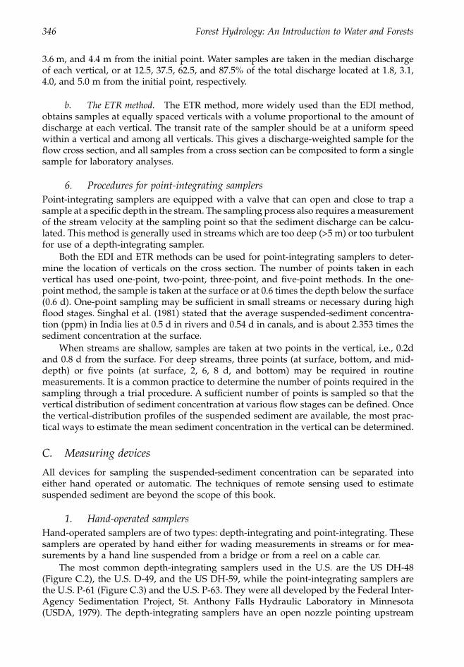
346 Forest Hydrology: An Introduction to Water and Forests
3.6 m, and 4.4 m from the initial point. Water samples are taken in the median dischargeof each vertical, or at 12.5, 37.5, 62.5, and 87.5% of the total discharge located at 1.8, 3.1,4.0, and 5.0 m from the initial point, respectively.
b. The ETR method.
The ETR method, more widely used than the EDI method,obtains samples at equally spaced verticals with a volume proportional to the amount ofdischarge at each vertical. The transit rate of the sampler should be at a uniform speedwithin a vertical and among all verticals. This gives a discharge-weighted sample for theflow cross section, and all samples from a cross section can be composited to form a singlesample for laboratory analyses.
6. Procedures for point-integrating samplers
Point-integrating samplers are equipped with a valve that can open and close to trap asample at a specific depth in the stream. The sampling process also requires a measurementof the stream velocity at the sampling point so that the sediment discharge can be calcu-lated. This method is generally used in streams which are too deep (>5 m) or too turbulentfor use of a depth-integrating sampler.
Both the EDI and ETR methods can be used for point-integrating samplers to deter-mine the location of verticals on the cross section. The number of points taken in eachvertical has used one-point, two-point, three-point, and five-point methods. In the one-point method, the sample is taken at the surface or at 0.6 times the depth below the surface(0.6 d). One-point sampling may be sufficient in small streams or necessary during highflood stages. Singhal et al. (1981) stated that the average suspended-sediment concentra-tion (ppm) in India lies at 0.5 d in rivers and 0.54 d in canals, and is about 2.353 times thesediment concentration at the surface.
When streams are shallow, samples are taken at two points in the vertical, i.e., 0.2dand 0.8 d from the surface. For deep streams, three points (at surface, bottom, and mid-depth) or five points (at surface, 2, 6, 8 d, and bottom) may be required in routinemeasurements. It is a common practice to determine the number of points required in thesampling through a trial procedure. A sufficient number of points is sampled so that thevertical distribution of sediment concentration at various flow stages can be defined. Oncethe vertical-distribution profiles of the suspended sediment are available, the most prac-tical ways to estimate the mean sediment concentration in the vertical can be determined.
C. Measuring devices
All devices for sampling the suspended-sediment concentration can be separated intoeither hand operated or automatic. The techniques of remote sensing used to estimatesuspended sediment are beyond the scope of this book.
1. Hand-operated samplers
Hand-operated samplers are of two types: depth-integrating and point-integrating. Thesesamplers are operated by hand either for wading measurements in streams or for mea-surements by a hand line suspended from a bridge or from a reel on a cable car.
The most common depth-integrating samplers used in the U.S. are the US DH-48(Figure C.2), the U.S. D-49, and the US DH-59, while the point-integrating samplers arethe U.S. P-61 (Figure C.3) and the U.S. P-63. They were all developed by the Federal Inter-Agency Sedimentation Project, St. Anthony Falls Hydraulic Laboratory in Minnesota(USDA, 1979). The depth-integrating samplers have an open nozzle pointing upstream
1363_ AppC_fm Page 346 Wednesday, December 4, 2002 7:47 AM
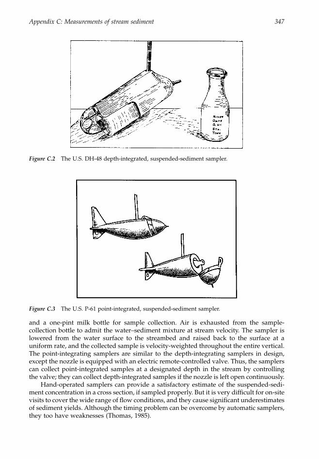
Appendix C: Measurements of stream sediment 347
and a one-pint milk bottle for sample collection. Air is exhausted from the sample-collection bottle to admit the water–sediment mixture at stream velocity. The sampler islowered from the water surface to the streambed and raised back to the surface at auniform rate, and the collected sample is velocity-weighted throughout the entire vertical.The point-integrating samplers are similar to the depth-integrating samplers in design,except the nozzle is equipped with an electric remote-controlled valve. Thus, the samplerscan collect point-integrated samples at a designated depth in the stream by controllingthe valve; they can collect depth-integrated samples if the nozzle is left open continuously.
Hand-operated samplers can provide a satisfactory estimate of the suspended-sedi-ment concentration in a cross section, if sampled properly. But it is very difficult for on-sitevisits to cover the wide range of flow conditions, and they cause significant underestimatesof sediment yields. Although the timing problem can be overcome by automatic samplers,they too have weaknesses (Thomas, 1985).
Figure C.2
The U.S. DH-48 depth-integrated, suspended-sediment sampler.
Figure C.3
The U.S. P-61 point-integrated, suspended-sediment sampler.
1363_ AppC_fm Page 347 Wednesday, December 4, 2002 7:47 AM
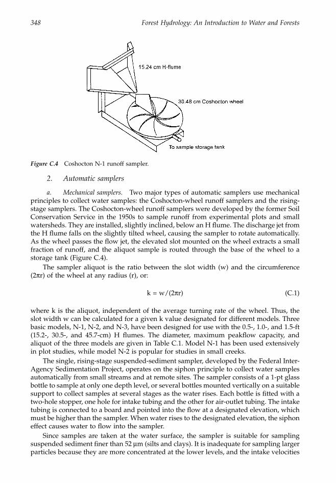
348 Forest Hydrology: An Introduction to Water and Forests
2. Automatic samplers
a. Mechanical samplers.
Two major types of automatic samplers use mechanicalprinciples to collect water samples: the Coshocton-wheel runoff samplers and the rising-stage samplers. The Coshocton-wheel runoff samplers were developed by the former SoilConservation Service in the 1950s to sample runoff from experimental plots and smallwatersheds. They are installed, slightly inclined, below an H flume. The discharge jet fromthe H flume falls on the slightly tilted wheel, causing the sampler to rotate automatically.As the wheel passes the flow jet, the elevated slot mounted on the wheel extracts a smallfraction of runoff, and the aliquot sample is routed through the base of the wheel to astorage tank (Figure C.4).
The sampler aliquot is the ratio between the slot width (w) and the circumference(2
p
r) of the wheel at any radius (r), or:
k = w/(2
p
r) (C.1)
where k is the aliquot, independent of the average turning rate of the wheel. Thus, theslot width w can be calculated for a given k value designated for different models. Threebasic models, N-1, N-2, and N-3, have been designed for use with the 0.5-, 1.0-, and 1.5-ft(15.2-, 30.5-, and 45.7-cm) H flumes. The diameter, maximum peakflow capacity, andaliquot of the three models are given in Table C.1. Model N-1 has been used extensivelyin plot studies, while model N-2 is popular for studies in small creeks.
The single, rising-stage suspended-sediment sampler, developed by the Federal Inter-Agency Sedimentation Project, operates on the siphon principle to collect water samplesautomatically from small streams and at remote sites. The sampler consists of a 1-pt glassbottle to sample at only one depth level, or several bottles mounted vertically on a suitablesupport to collect samples at several stages as the water rises. Each bottle is fitted with atwo-hole stopper, one hole for intake tubing and the other for air-outlet tubing. The intaketubing is connected to a board and pointed into the flow at a designated elevation, whichmust be higher than the sampler. When water rises to the designated elevation, the siphoneffect causes water to flow into the sampler.
Since samples are taken at the water surface, the sampler is suitable for samplingsuspended sediment finer than 52
m
m (silts and clays). It is inadequate for sampling largerparticles because they are more concentrated at the lower levels, and the intake velocities
Figure C.4
Coshocton N-1 runoff sampler.
1363_ AppC_fm Page 348 Wednesday, December 4, 2002 7:47 AM
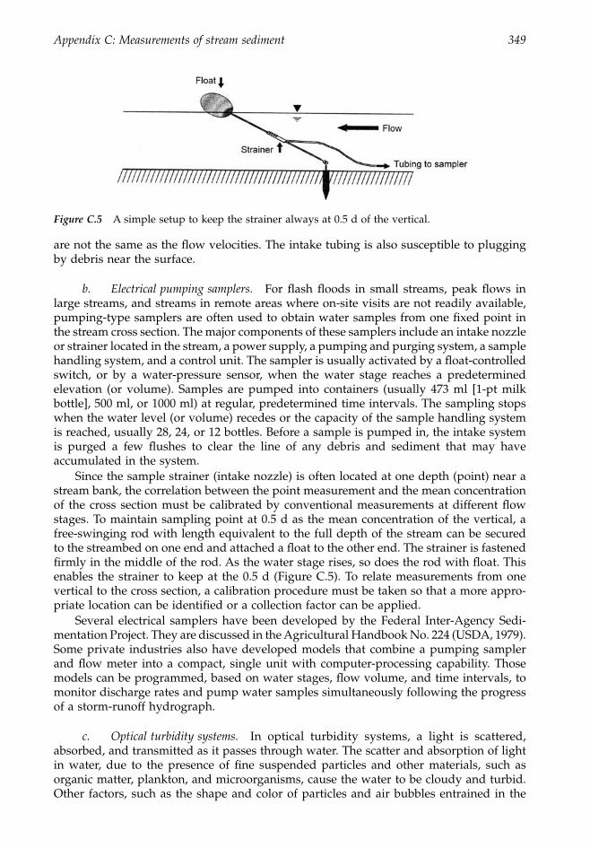
Appendix C: Measurements of stream sediment 349
are not the same as the flow velocities. The intake tubing is also susceptible to pluggingby debris near the surface.
b. Electrical pumping samplers.
For flash floods in small streams, peak flows inlarge streams, and streams in remote areas where on-site visits are not readily available,pumping-type samplers are often used to obtain water samples from one fixed point inthe stream cross section. The major components of these samplers include an intake nozzleor strainer located in the stream, a power supply, a pumping and purging system, a samplehandling system, and a control unit. The sampler is usually activated by a float-controlledswitch, or by a water-pressure sensor, when the water stage reaches a predeterminedelevation (or volume). Samples are pumped into containers (usually 473 ml [1-pt milkbottle], 500 ml, or 1000 ml) at regular, predetermined time intervals. The sampling stopswhen the water level (or volume) recedes or the capacity of the sample handling systemis reached, usually 28, 24, or 12 bottles. Before a sample is pumped in, the intake systemis purged a few flushes to clear the line of any debris and sediment that may haveaccumulated in the system.
Since the sample strainer (intake nozzle) is often located at one depth (point) near astream bank, the correlation between the point measurement and the mean concentrationof the cross section must be calibrated by conventional measurements at different flowstages. To maintain sampling point at 0.5 d as the mean concentration of the vertical, afree-swinging rod with length equivalent to the full depth of the stream can be securedto the streambed on one end and attached a float to the other end. The strainer is fastenedfirmly in the middle of the rod. As the water stage rises, so does the rod with float. Thisenables the strainer to keep at the 0.5 d (Figure C.5). To relate measurements from onevertical to the cross section, a calibration procedure must be taken so that a more appro-priate location can be identified or a collection factor can be applied.
Several electrical samplers have been developed by the Federal Inter-Agency Sedi-mentation Project. They are discussed in the Agricultural Handbook No. 224 (USDA, 1979).Some private industries also have developed models that combine a pumping samplerand flow meter into a compact, single unit with computer-processing capability. Thosemodels can be programmed, based on water stages, flow volume, and time intervals, tomonitor discharge rates and pump water samples simultaneously following the progressof a storm-runoff hydrograph.
c. Optical turbidity systems.
In optical turbidity systems, a light is scattered,absorbed, and transmitted as it passes through water. The scatter and absorption of lightin water, due to the presence of fine suspended particles and other materials, such asorganic matter, plankton, and microorganisms, cause the water to be cloudy and turbid.Other factors, such as the shape and color of particles and air bubbles entrained in the
Figure C.5
A simple setup to keep the strainer always at 0.5 d of the vertical.
1363_ AppC_fm Page 349 Wednesday, December 4, 2002 7:47 AM
350 Forest Hydrology: An Introduction to Water and Forests
water also significantly affect light absorption and scattering. Thus,
turbidity
refers to therelative amount of light that is scattered or absorbed by a fluid. It is an optical propertyof the fluid and can be measured by turbidity meters on water samples or monitoredcontinuously by a turbidity system.
Historically, the determination of turbidity has been based on the Jackson candleturbidimeter. It is a measure of the ratio of the light transmitted through the water samplein a straight line to the incident light in Jackson turbidity units (JTU). However, the Jacksonturbidimeter is unable to detect turbidity below 25 JTU and dark-colored particles. Thishas led to the widespread replacement of Jackson candle turbidimeters with photoelectricnephelometers since the 1970s (MacDonald et al., 1991; APHA, 1989). The nephelometermeasures the ratio of intensity of light scattered at right angles by the water sample tothe intensity of light scattered by a standard reference suspension under the same condi-tions, in nephelometric turbidity units (NTU). Formazin polymer is used as the turbiditystandard suspension for calibrations. A higher amount of suspended matter will causethe intensity of scattered light to be higher and gives a higher value of turbidity. Becauseof the differences in measurement techniques, there is no valid basis for the calibrationbetween NTUs and JTUs (APHA, 1989).
A continuous turbidity-monitoring system usually consists of a pumping and recir-culating system for water samples from the stream, sedimentation chamber, and detectorand recording devices (Grobler and Weaver, 1981; WMO, 1981). Some turbidmeter systemsare able to link a number of sensors into a high-level, two-way communications networkthat provides real-time monitoring from a central station (Hach, 1998). Also, multiparam-eter instruments with submersible sondes that can accommodate a turbidity sensor, com-monly referred to as water-quality probe or turbidity probe, can be used in conjunctionwith a datalogger for
in situ
measurements. Most multiparameter instruments are micro-processor-based, with the calibration parameters stored in instrument memory. The stan-dards for turbidity are user-selectable in some probes, but are internally established insome others that cannot be changed. Detailed information on turbidity measurements isgiven by the USGS (Wilde and Radtke, 1998).
Turbidity is relatively easy to measure in the field or laboratory, whereas suspendedsediments require lengthy procedures in the field-sample collection and laboratory anal-ysis. Also, suspended sediments are not easy to collect in small mountainous watershedswhere suspended-sediment concentrations and streamflow can change rapidly. Becausesuspended sediment is the most important factor affecting stream turbidity (Beschta, 1980),a logical assumption is that suspended-sediment concentration can be estimated by tur-bidity. Studies have showed that meaningful relationships can be established in someareas (Kunkle and Comer, 1971), but not in all areas (Weigel, 1984), and that such rela-tionships vary by site, within storms, and between storms (Beschta, 1980). In the PacificNorthwest, MacDonald et al., (1991) stated that about 80% of the variability of the sus-pended-sediment concentration is attributable to turbidity. The variation in sediment–tur-bidity relationships is probably due to the nature of turbidity and its contributing sources.Other factors such as particle shape, organic compounds, algae, color, and phytoplanktonalso affect the scattering and absorption of light in water. Organic substances in streamsvary in seasons, between the rising and recession stages in runoff events, within a water-shed, and among watersheds. Prediction equations should therefore be developed on asite-by-site basis.
d. Acoustic Doppler current profiler (ADCP).
With the ADCP, sound bursts aretransmitted into the water column; echoes are produced when the sound bursts hit sus-pended particles carried by water currents. The ADCP senses simultaneously in fourorthogonal directions in which particles moving toward the instrument record greaterfrequencies than those moving away from the instrument. The lag times and frequencies
1363_ AppC_fm Page 350 Wednesday, December 4, 2002 7:47 AM
Appendix C: Measurements of stream sediment 351
of these echoes due to the Doppler shift are detected by the monitoring system to estimatesuspended-solids concentration. ADCPs have the ability to measure flow velocities andsuspended-solids concentrations throughout the water column and across the streamchannel.
e. Radioactive turbiometric gages.
In streams with sediment concentrations inexcess of 100g/l, nuclear gages are the most suitable means for
in situ
measurements.These gages can monitor a wide range of sediment concentrations and resist bedloadtransport consisting of boulder-size material. They are fully automatic, are independentof the color and diameter of the suspended particles, and practically do not disturb thefluid (Tazioli, 1981).
Nuclear suspended-sediment gages measure the attenuation of radiation intensity(gamma rays) either back scattered or absorbed by the water–sediment mixture. Anartificial source of radiation (
137
Cs,
60
Co,
109
Cd, or
241
Am) is emitted to the water, and itsattenuation, due to the sediment concentration, is detected by a counter installed in thedownstream side of the gage or in a separate rod. Counts are converted directly intosediment concentrations by comparison to reference samples in a precalibration proce-dure. The volume of measurements, varying from a few liters to several m
3
, depends onthe source–detector distance, the radiation energy, and the time interval in counting.Gages developed in China have shown excellent agreement with the conventional methodof sampling for sediment concentration from 15 to 500 kg/m
3
in the Yellow River (Luet al., 1981).
D. Calculations
The collection of suspended-sediment water samples and the measurement of flow dis-charge are often conducted simultaneously in a few verticals along a stream cross section.The collected water samples are brought to the laboratory for sediment-concentrationdeterminations and are expressed in mass/volume (mg/l). The suspended-sediment con-centration and discharge rate are then used to calculate the suspended load.
1. Suspended-sediment load for a cross section
The suspended-sediment concentration (c
s
) in each vertical is multiplied by its meandischarge rate (q, m
3
/sec) to obtain suspended-sediment load, or yield, (q
SL
) in mass/timefor that vertical. In common practice, c
s
is in mg/l, q in m
3
/sec, and q
SL
in t/d calculated by:
q
SL
= 0.0864(q)(c
s
) (C.2)
The constant 0.0864 converts the units from mg/sec to t/d, assuming q and c
s
stay thesame for the day. Summing up all values of q
SL
in each vertical yields the total suspended-sediment load for the cross section, M
SL
, or:
Q
SL
= (q
SL
)
1
+ (q
SL
)
2
+ (q
SL
)
3
+
◊◊◊
+ (q
SL
)
n
(C.3)
2. Mean suspended-sediment concentration
For the mean suspended-sediment concentration (C
s
) of the entire cross section, all valuesof c
s
need to be weighted by each corresponding discharge rate as a percent of the totaldischarge rate for the entire cross section, or:
C
s
= [(c
s
)
1
(q
1
) + (c
s
)
2
(q
2
) + (c
s
)
3
(q
3
) +
◊◊◊
]/[q
1
+ q
2
+ q
3
+
◊◊◊
] (C.4)
1363_ AppC_fm Page 351 Wednesday, December 4, 2002 7:47 AM
352 Forest Hydrology: An Introduction to Water and Forests
where the numerical subscripts 1, 2, 3, etc. refer to the different sampling verticals. Theyalso can refer to different time intervals if mean concentrations for a day or other periodsof time are needed.
3. Suspended-sediment load for a runoff event
Often more water samples are collected during a major runoff event. In a runoff event,water samples are usually not collected at an equal time interval along the rise and fallof the discharge hydrograph, and the sediment load sampled at time 1 needs to beaveraged with sediment load sampled at time 2 for that time interval. Thus, averages ofsediment load are calculated for all time intervals for the entire runoff event. The sum-mation of the averages of the suspended-sediment load for all time intervals is the totalsuspended-sediment load for the runoff event. In equation form,
Q
SL
=
Â
[[(c
s
)
1
(q
1
) + (c
s
)
2
(q
2
)](t
1–2
)/2 + [(c
s
)
2
(q
2
) + (c
s
)
3
(q
3
)](t
2–3
)/2 +
◊◊◊
] (C.5)
where the numerical subscripts 1, 2, 3, etc. refer to the sampling period at time 1, 2, 3, etc.Thus, t
1
-
2
is the time interval between periods 1 and 2.
II. Bedload
Bedload is the sediment transported downstream by sliding, saltation, and rolling alongthe streambed. The transported material remains in contact with the streambed. Forpractical purposes, particles with a diameter greater than 1.0 mm are transported asbedload, while diameters less than 0.1 mm are transported as suspended load, and diam-eters between 1.0 and 0.1 mm can be transported either as bedload or suspended load,depending on the hydraulic conditions (MacDonald et al., 1991). Particles that are lessthan 0.0625 mm in diameter will be carried in suspension by the stream as washload andmay never settle out.
Bedload transport can be further differentiated into sand transport (1 to 2 mm) andcoarse bedload transport (2 mm to boulders). Sand transport is more controlled by thehydraulic conditions and can be initiated in ordinary flows, while coarse bedload is usuallylimited to high flows that occur less frequently (Bunte, 1996). The amount and size ofbedloads are important factors affecting channel morphology, streambed configuration,reservoir storage capacity, and aquatic habitat. Generally, fine material tends to fill up theinterstitial spaces between large particles, causing less habitat space to be available forjuvenile fish and macroinvertebrates, and lower dissolved-oxygen levels for benthic com-munities and salmon spawning.
A. Bedload variation
Bedload transport depends greatly on stream discharge, but not in a predictable way. Itmoves in irregular waves and sheets due to the streambed configuration and the variationin shear stress of the flow. Thus, the transport varies considerably with time and acrossthe section. In fact, bedload generally occurs in part of the stream cross section only, exceptduring floods. It tends to be higher during the recession stage than at the rising stage ofa runoff event, and the majority is transported during the very few largest flows in a givenyear. There is no consistent relationship between bedload and discharge or betweenbedload and suspended load (Williams, 1989).
As an example of the temporal variation, Figure C.6 is a plot of bedload-transportrate sampled consecutively with a Halley-Smith sampler in a 3-minute interval betweensamples on a sand-bed stream in western Tennessee (Carey, 1985). These samples were
1363_ AppC_fm Page 352 Wednesday, December 4, 2002 7:47 AM
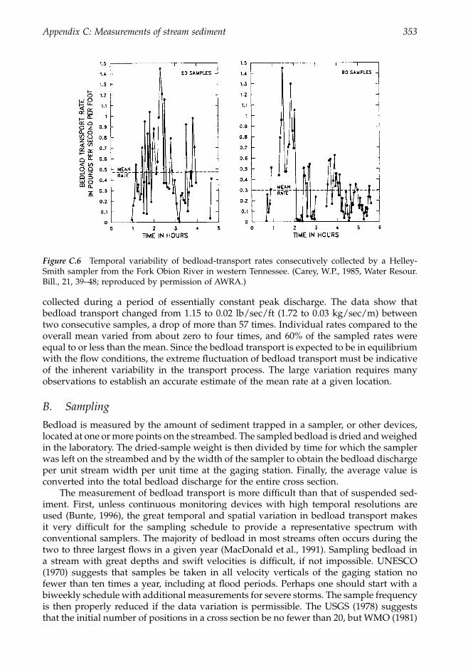
Appendix C: Measurements of stream sediment 353
collected during a period of essentially constant peak discharge. The data show thatbedload transport changed from 1.15 to 0.02 lb/sec/ft (1.72 to 0.03 kg/sec/m) betweentwo consecutive samples, a drop of more than 57 times. Individual rates compared to theoverall mean varied from about zero to four times, and 60% of the sampled rates wereequal to or less than the mean. Since the bedload transport is expected to be in equilibriumwith the flow conditions, the extreme fluctuation of bedload transport must be indicativeof the inherent variability in the transport process. The large variation requires manyobservations to establish an accurate estimate of the mean rate at a given location.
B. Sampling
Bedload is measured by the amount of sediment trapped in a sampler, or other devices,located at one or more points on the streambed. The sampled bedload is dried and weighedin the laboratory. The dried-sample weight is then divided by time for which the samplerwas left on the streambed and by the width of the sampler to obtain the bedload dischargeper unit stream width per unit time at the gaging station. Finally, the average value isconverted into the total bedload discharge for the entire cross section.
The measurement of bedload transport is more difficult than that of suspended sed-iment. First, unless continuous monitoring devices with high temporal resolutions areused (Bunte, 1996), the great temporal and spatial variation in bedload transport makesit very difficult for the sampling schedule to provide a representative spectrum withconventional samplers. The majority of bedload in most streams often occurs during thetwo to three largest flows in a given year (MacDonald et al., 1991). Sampling bedload ina stream with great depths and swift velocities is difficult, if not impossible. UNESCO(1970) suggests that samples be taken in all velocity verticals of the gaging station nofewer than ten times a year, including at flood periods. Perhaps one should start with abiweekly schedule with additional measurements for severe storms. The sample frequencyis then properly reduced if the data variation is permissible. The USGS (1978) suggeststhat the initial number of positions in a cross section be no fewer than 20, but WMO (1981)
Figure C.6
Temporal variability of bedload-transport rates consecutively collected by a Helley-Smith sampler from the Fork Obion River in western Tennessee. (Carey, W.P., 1985, Water Resour.Bill., 21, 39–48; reproduced by permission of AWRA.)
1363_ AppC_fm Page 353 Wednesday, December 4, 2002 7:47 AM
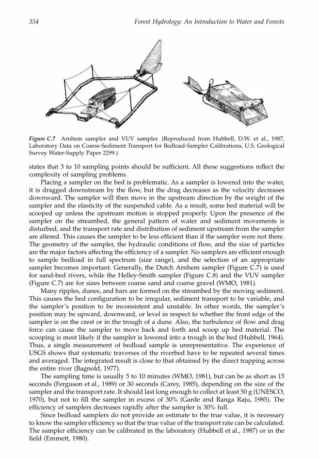
354 Forest Hydrology: An Introduction to Water and Forests
states that 3 to 10 sampling points should be sufficient. All these suggestions reflect thecomplexity of sampling problems.
Placing a sampler on the bed is problematic. As a sampler is lowered into the water,it is dragged downstream by the flow, but the drag decreases as the velocity decreasesdownward. The sampler will then move in the upstream direction by the weight of thesampler and the elasticity of the suspended cable. As a result, some bed material will bescooped up unless the upstream motion is stopped properly. Upon the presence of thesampler on the streambed, the general pattern of water and sediment movements isdisturbed, and the transport rate and distribution of sediment upstream from the samplerare altered. This causes the sampler to be less efficient than if the sampler were not there.The geometry of the sampler, the hydraulic conditions of flow, and the size of particlesare the major factors affecting the efficiency of a sampler. No samplers are efficient enoughto sample bedload in full spectrum (size range), and the selection of an appropriatesampler becomes important. Generally, the Dutch Arnhem sampler (Figure C.7) is usedfor sand-bed rivers, while the Helley-Smith sampler (Figure C.8) and the VUV sampler(Figure C.7) are for sizes between coarse sand and coarse gravel (WMO, 1981).
Many ripples, dunes, and bars are formed on the streambed by the moving sediment.This causes the bed configuration to be irregular, sediment transport to be variable, andthe sampler’s position to be inconsistent and unstable. In other words, the sampler’sposition may be upward, downward, or level in respect to whether the front edge of thesampler is on the crest or in the trough of a dune. Also, the turbulence of flow and dragforce can cause the sampler to move back and forth and scoop up bed material. Thescooping is most likely if the sampler is lowered into a trough in the bed (Hubbell, 1964).Thus, a single measurement of bedload sample is unrepresentative. The experience ofUSGS shows that systematic traverses of the riverbed have to be repeated several timesand averaged. The integrated result is close to that obtained by the direct trapping acrossthe entire river (Bagnold, 1977).
The sampling time is usually 5 to 10 minutes (WMO, 1981), but can be as short as 15seconds (Ferguson et al., 1989) or 30 seconds (Carey, 1985), depending on the size of thesampler and the transport rate. It should last long enough to collect at least 50 g (UNESCO,1970), but not to fill the sampler in excess of 30% (Garde and Ranga Raju, 1985). Theefficiency of samplers decreases rapidly after the sampler is 30% full.
Since bedload samplers do not provide an estimate to the true value, it is necessaryto know the sampler efficiency so that the true value of the transport rate can be calculated.The sampler efficiency can be calibrated in the laboratory (Hubbell et al., 1987) or in thefield (Emmett, 1980).
Figure C.7
Arnhem sampler and VUV sampler. (Reproduced from Hubbell, D.W. et al., 1987,Laboratory Data on Coarse-Sediment Transport for Bedload-Sampler Calibrations, U.S. GeologicalSurvey Water-Supply Paper 2299.)
1363_ AppC_fm Page 354 Wednesday, December 4, 2002 7:47 AM
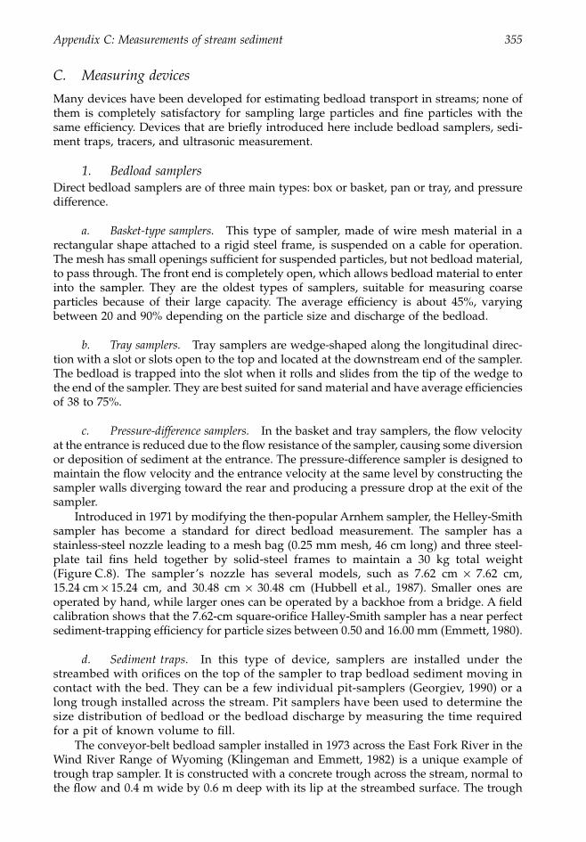
Appendix C: Measurements of stream sediment 355
C. Measuring devices
Many devices have been developed for estimating bedload transport in streams; none ofthem is completely satisfactory for sampling large particles and fine particles with thesame efficiency. Devices that are briefly introduced here include bedload samplers, sedi-ment traps, tracers, and ultrasonic measurement.
1. Bedload samplers
Direct bedload samplers are of three main types: box or basket, pan or tray, and pressuredifference.
a. Basket-type samplers.
This type of sampler, made of wire mesh material in arectangular shape attached to a rigid steel frame, is suspended on a cable for operation.The mesh has small openings sufficient for suspended particles, but not bedload material,to pass through. The front end is completely open, which allows bedload material to enterinto the sampler. They are the oldest types of samplers, suitable for measuring coarseparticles because of their large capacity. The average efficiency is about 45%, varyingbetween 20 and 90% depending on the particle size and discharge of the bedload.
b. Tray samplers.
Tray samplers are wedge-shaped along the longitudinal direc-tion with a slot or slots open to the top and located at the downstream end of the sampler.The bedload is trapped into the slot when it rolls and slides from the tip of the wedge tothe end of the sampler. They are best suited for sand material and have average efficienciesof 38 to 75%.
c. Pressure-difference samplers. In the basket and tray samplers, the flow velocityat the entrance is reduced due to the flow resistance of the sampler, causing some diversionor deposition of sediment at the entrance. The pressure-difference sampler is designed tomaintain the flow velocity and the entrance velocity at the same level by constructing thesampler walls diverging toward the rear and producing a pressure drop at the exit of thesampler.
Introduced in 1971 by modifying the then-popular Arnhem sampler, the Helley-Smithsampler has become a standard for direct bedload measurement. The sampler has astainless-steel nozzle leading to a mesh bag (0.25 mm mesh, 46 cm long) and three steel-plate tail fins held together by solid-steel frames to maintain a 30 kg total weight(Figure C.8). The sampler’s nozzle has several models, such as 7.62 cm ¥ 7.62 cm,15.24 cm ¥ 15.24 cm, and 30.48 cm ¥ 30.48 cm (Hubbell et al., 1987). Smaller ones areoperated by hand, while larger ones can be operated by a backhoe from a bridge. A fieldcalibration shows that the 7.62-cm square-orifice Halley-Smith sampler has a near perfectsediment-trapping efficiency for particle sizes between 0.50 and 16.00 mm (Emmett, 1980).
d. Sediment traps. In this type of device, samplers are installed under thestreambed with orifices on the top of the sampler to trap bedload sediment moving incontact with the bed. They can be a few individual pit-samplers (Georgiev, 1990) or along trough installed across the stream. Pit samplers have been used to determine thesize distribution of bedload or the bedload discharge by measuring the time requiredfor a pit of known volume to fill.
The conveyor-belt bedload sampler installed in 1973 across the East Fork River in theWind River Range of Wyoming (Klingeman and Emmett, 1982) is a unique example oftrough trap sampler. It is constructed with a concrete trough across the stream, normal tothe flow and 0.4 m wide by 0.6 m deep with its lip at the streambed surface. The trough
1363_ AppC_fm Page 355 Wednesday, December 4, 2002 7:47 AM
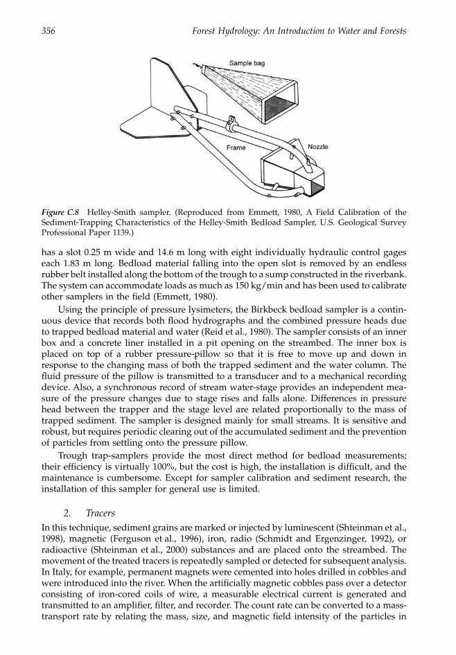
356 Forest Hydrology: An Introduction to Water and Forests
has a slot 0.25 m wide and 14.6 m long with eight individually hydraulic control gageseach 1.83 m long. Bedload material falling into the open slot is removed by an endlessrubber belt installed along the bottom of the trough to a sump constructed in the riverbank.The system can accommodate loads as much as 150 kg/min and has been used to calibrateother samplers in the field (Emmett, 1980).
Using the principle of pressure lysimeters, the Birkbeck bedload sampler is a contin-uous device that records both flood hydrographs and the combined pressure heads dueto trapped bedload material and water (Reid et al., 1980). The sampler consists of an innerbox and a concrete liner installed in a pit opening on the streambed. The inner box isplaced on top of a rubber pressure-pillow so that it is free to move up and down inresponse to the changing mass of both the trapped sediment and the water column. Thefluid pressure of the pillow is transmitted to a transducer and to a mechanical recordingdevice. Also, a synchronous record of stream water-stage provides an independent mea-sure of the pressure changes due to stage rises and falls alone. Differences in pressurehead between the trapper and the stage level are related proportionally to the mass oftrapped sediment. The sampler is designed mainly for small streams. It is sensitive androbust, but requires periodic clearing out of the accumulated sediment and the preventionof particles from settling onto the pressure pillow.
Trough trap-samplers provide the most direct method for bedload measurements;their efficiency is virtually 100%, but the cost is high, the installation is difficult, and themaintenance is cumbersome. Except for sampler calibration and sediment research, theinstallation of this sampler for general use is limited.
2. TracersIn this technique, sediment grains are marked or injected by luminescent (Shteinman et al.,1998), magnetic (Ferguson et al., 1996), iron, radio (Schmidt and Ergenzinger, 1992), orradioactive (Shteinman et al., 2000) substances and are placed onto the streambed. Themovement of the treated tracers is repeatedly sampled or detected for subsequent analysis.In Italy, for example, permanent magnets were cemented into holes drilled in cobbles andwere introduced into the river. When the artificially magnetic cobbles pass over a detectorconsisting of iron-cored coils of wire, a measurable electrical current is generated andtransmitted to an amplifier, filter, and recorder. The count rate can be converted to a mass-transport rate by relating the mass, size, and magnetic field intensity of the particles in
Figure C.8 Helley-Smith sampler. (Reproduced from Emmett, 1980, A Field Calibration of theSediment-Trapping Characteristics of the Helley-Smith Bedload Sampler, U.S. Geological SurveyProfessional Paper 1139.)
1363_ AppC_fm Page 356 Wednesday, December 4, 2002 7:47 AM
Appendix C: Measurements of stream sediment 357
the sample to signals produced from the detector through a precalibration procedure,(Ergenzinger and Conrady, 1982). This technique can also obtain information such as themovement of tracer particles in relation to various hydraulic conditions. There are manystreams in andesitic and basaltic terrain or with geologic formations around the worldthat have natural sources of magnetic material. Ergenzinger and Custer (1983) showedthat the technique also could be applied to estimate bedload transport by using naturallymagnetic tracers in Montana. More recent developments in the magnetic tracer techniqueare given by Spieker and Ergenzinger (1990).
3. Acoustic and ultrasonic measurementIn sand-bed streams where the movement of bedload characteristically forms many well-defined dunes, the ultrasonic technique can be used to monitor changes in vertical depthalong a selected cross section of the stream. Thus, data on the profile of the dunes andthe velocity of their movement can be obtained. The sand-dune profile can be used tocompute the sand-dune area, and multiplying the area by the mean velocity of the sand-dune movement gives the bedload discharge per unit width of the stream channel (WMO,1981). Ultrasonic gages have also been used to monitor the height and volume of bed loadmaterial transported to an open storage area along the stream channel (Lenzi et al., 1990).
In coarse-grained streams, the moving and colliding particles cause clicking noiseswhen they hit an acoustic (hydrophonic) detector consisting of a metal sheet installed onthe streambed. A microphone is built into the detector to amplify the noises, which aretransmitted to a headphone or a magnetic-tape recorder. The frequency of noises givessome qualitative information on the intensity of bedload movement (Banziger and Burch,1990) and can help to select bedload sampling points along a cross section.
D. Calculations
Measurements for bedload discharge by a sampler are made at several verticals of thestream cross section. Bedload discharge at each measurement point is calculated by:
qBL = (e) (C.6)
where
qBL = bedload discharge in mass per unit width per unit timeM = mass of the bedload caught by the samplerw = orifice width of the samplert = sampling duration at the measuring pointe = efficiency of the sampler
Total bedload discharge (QBL, in mass/time) for the cross section is calculated by:
QBL = Â[(qBL1 + qBL2)(d1–2)/2 + (qBL + qBL)(d2–3)/2 + ◊◊◊] (C.7)
where qBL1 = bedload discharge at measuring point 1 calculated by Equation C.6, andd1–2 = distance between measuring points 1 and 2.
Mwt------
Ë ¯Ê �
1363_ AppC_fm Page 357 Wednesday, December 4, 2002 7:47 AM
358 Forest Hydrology: An Introduction to Water and Forests
ReferencesAPHA, 1989, Standard Methods for the Examination of Water and Wastewater, 17th ed., Amer. Public
Health Assoc., Washington, D.CBagnold, R.A., 1977, Bed load transport by natural rivers, Water Resour. Res., 13, 303–312.Banziger, R. and Burch, H., 1990, Acoustic sensors (hydrophones) as indicators for bed load transport
in a mountain torrent, in Hydrology in Mountainous Regions, IAHS, pp. 207–214.Beschta, R.L., 1980, Turbidity and suspended sediment relationships, in Sym. Watershed Management,
Vol. I, ASCE, pp. 271–282.Bonta, J. V., 2000, Impact of coal surface mining and reclamation on suspended sediment in three
Ohio watersheds, J. Am. Water Resour. Assoc., 36, 869–887.Bunte, K., 1996, Analyses of the Temporal Variation of Coarse Bedload Transport and its Grain Size
Distribution, Gen. Tech. Rep. RM-GTR-288, USDA Forest Service, Rocky Mountain Forestand Range Exp. Sta.
Carey, W.P., 1985, Variability in measured bedload-transport rates, Water Resour. Bull., 21, 39–48.Emmett, 1980, A Field Calibration of the Sediment-Trapping Characteristics of the Helley-Smith
Bedload Sampler, U.S. Geological Survey Professional Paper 1139.Ergenzinger, P.J. and Conrady, J., 1982, A new tracer technique for measuring bedload in natural
channels, Vatena, 9, 77–90.Ergenzinger, P.J., and Custer, S.G., 1983, Determination of bedload transport using naturally mag-
netic tracers: first experiences at Squaw Creek, Gallatin County, Montana, Water Resour. Res.,19, 187–193.
Ferguson, R.I., 1986, River loads underestimated by rating curves, Water Resour. Res., 22, 74–76.Ferguson, R. et al., 1996, Field evidence for rapid downstream running of river gravels through
selective transport, Geology, 24, 179–182.Ferguson, R.I., Prestegaard, K.L., and Ashworth, P.J., 1989, Influence of sand on hydraulics and
gravel transport in a braided gravel bed river, Water Resour. Res., 25, 635–643.Garde, R.J. and Ranga Raju, K.G., 1985, Mechanics of Sediment Transportation and Alluvial Stream
Problems, John Wiley & Sons, New York.Georgiev, B.V., 1990, Reliability of bed load measurements in mountain rivers, in Hydrology in
Mountainous Regions, IAHS, pp. 263–270.Gordon, N.D., McMahon, T.A., and Finlayson, B.L., 1992, Stream Hydrology, An Introduction for
Ecologists, John Wiley & Sons, New York.Grobler, D.C. and Weaver, A. van B., 1981, Continuous measurement of suspended sediment in
rivers by means of a double beam turbidity meter, in Erosion and Sediment Transport Measure-ment, Proc. of the Florence Sym., IAHS, pp. 97–104.
Guy, H.P. and Norman, V.W., 1970, Field methods for measurement of fluvial sediment, in Techniquesof Water-Resources Investigations, U.S. Geological Survey, Chapter C2, Book 3, Applicationsof Hydraulics. U.S. Government Printing Office, Washington, D.C.
HACH, 1998, Products and Analysis, HACH Company, Loveland, CO.Hubbell, D.W., 1964, Apparatus and Techniques for Measuring Bedload, U.S. Geological Survey
Water-Supply Paper 1748.Hubbell, D.W. et al., 1987, Laboratory Data on Coarse-Sediment Transport for Bedload-Sampler
Calibrations, U.S. Geological Survey Water-Supply Paper 2299.Klingeman, P.C. and Emmett, W.W., 1982, Gravel bedload transport processes, in Gravel Bed River.
Fluvial Processes, Engineering and Management, Hey, R.D., Bathurst, J.C., and Thorne, C.R.,eds., John Wiley & Sons, New York, pp. 141–179.
Kunkle, S.H. and Comer, G.H., 1971, Estimating suspended sediment concentration in streams byturbidity measurements, J. Soil Water Conserv., 26, 18–20.
Lenzi, M.A., Marchi, L., and Scussel, G.R., 1990, Measurement of coarse sediment transport in asmall alpine stream, in Hydrology in Mountainous Regions, IAHS, pp. 283–290.
Lu, Z. et al., 1981, The development of nuclear sediment concentration gauges for use on the YellowRiver, in Erosion and Sediment Transport Measurement, Proc. of the Florence Sym., IAHS, pp.83–90.
1363_ AppC_fm Page 358 Wednesday, December 4, 2002 7:47 AM
Appendix C: Measurements of stream sediment 359
MacDonald, L.H., Smart, A.W., and Wissmar, R.C., 1991, Monitoring Guidelines to Evaluate Effectsof Forestry Activities on Streams in the Pacific Northwest and Alaska, EPA/910/9–91–001.
Parsons,Reid, I., Layman, J.T., and Frostick, L.E., 1980, The continuous measurement of bedload discharge,
J. Hydraulic Res., 18, 243–249.Schmidt, K.H. and Ergenzinger, P., 1992, Bedload entrainment, travel lengths, step lengths, set
periods, studied with passive (iron, magnetic) and active (radio) tracer techniques, Earth Surf.Process. Landforms, 17, 147–165.
Shteinman, B.S. et al., 1998, A modified fluorescent tracer approach for studies of sediment dynamics,Isr. J. Earth Sci. 46, 18–31.
Shteinman, B., Wynne, D., and Kamenir, Y., 2000, Study of sediment dynamics in the Jordan River-Lake Kinneret contact zone using tracer methods, in The Hydrology-Geomorphology Interface:Rainfall, Floods, Sedimentation, Land Use, IAHS, pp. 275–284.
Singhal, H.S.S., Goshi, G.C., and Verma, R.S., 1981, Sediment sampling in rivers and canals, in Erosionand Sediment Transport Measurement, Proc. of the Florence Sym., IAHS, pp. 169–175.
Spieker, R. and Ergenzinger, P.J., 1990, New developments in measuring bedload by the magnetictracer technique, in Erosion, Transport, and Deposition Processes, IAHS, pp. 171–180.
Tazioli, G.S., 1981, Nuclear techniques for measuring sediment transport in natural streams —examples from instrumented basins, in Erosion and Sediment Transport Measurement, Proc. ofthe Florence Sym., IAHS, pp. 63–81.
Thomas, R.B., 1985, Measuring suspended sediment in small mountain streams, Gen. Tech. Rep.PSW-83, U.S. Forest Service, Pacific Southwest Forest and Range Exp. Sta.
UNESCO, 1970, Representative and Experimental Basin, an International Guide for Research and Practice,Toebes, C. and Ouryvaev, V., Eds., UNESCO, Paris.
UNESCO, 1982, Sedimentation Problems in River Basins, Proj. 5.3 of the International Hydro.Programme, UNESCO, Paris.
USDA, 1979, Field Manual for Research in Agricultural Hydrology, Agr. Handbook No. 224, U.S. Dept.Agr., Washington, D.C.
USGS, 1978, National Handbook of Recommended Methods for Water-Data Acquisition, 1–100.Walling, D.E. and Webb, B.W., 1981, The reliability of suspended sediment load data, in Erosion and
Sediment Transport Measurement, Proc. Florence Sym., IAHS, pp.177–194.Weigel, J.F., 1984, Turbidity and Suspended Sediment in the Jordan River, Salt Lake County, Utah,
USGS Water-Resour. Invest. Rep. 84–4019.Wilde, F.D. and Radtke, D.B., Eds., 1998, National Field Manual for the Collection of Water-Quality Data,
U.S. Geological Survey.Williams, G.P., 1989, Proportion of bedload to total sediment load in rivers, Eos, 70, 1106.WMO, 1981, Measurement of River Sediments, World Meteoro. Organ. Operational Hydrology Rep.
No. 16, WMO-No. 561, Geneva, Switzerland.
1363_ AppC_fm Page 359 Wednesday, December 4, 2002 7:47 AM

1363_ AppC_fm Page 360 Wednesday, December 4, 2002 7:47 AM

361
Index
A
Ablation, 151rates, 141
Absolute density, 39Absolute humidity, 132Acceleration, gravity and, 42Acid deposition, 127–128Acid mine drainage, 100Acoustic Doppler current profiler, 327, 350–351Acoustic flowmeters, 326–327Adhesion, molecular, 45Aerodynamic resistance, 137Agricultural Disaster Assistance, 97Agricultural irrigation, 17.
See also
Irrigationcrop efficient, 166
Agricultural Research Service, 243Agriculture Hydrology, 29Agroforestry, 124Agrohydrology, 31Air
pollution, 127–128thermal conductivity, 41
Albedo, 155, 156of natural surfaces, 156
Alcohol, 50Algae, 219Alluvial fan, 258Alter shield, 312Amazon Basin, 146Amazon River, 62Anemometers, hot-wire, 325Angiospermae, 111Annual potential insolation index, 196Antarctic regions, 60Antitranspirants, 87Aquatic ecosystems, 6Aquatic plants, 34Aquifer recharge, 6Archimedes' principle, 44, 291Arctic Ocean, 59Arctic regions, 60Arnhem sampler, 354Assyria, 2Ataturk Dam, 16
Atlantic Ocean, 59Atmosphere, 58, 119
heat balance, 71–72longwave radiation from, 51moisture, 132–133
magnitude, 132measures, 132–133saturation deficit, 133
solar radiation from, 51thermal conductivity, 41
Avalanches, 3, 122, 259
B
Babylon, 2Baobab trees, 86Baseflow, 176Bay estuaries, 19Benthos, 8Berghaus, Heinrich, 26Bernoulli equation, 43"Best Available Technology," 102"Best management practices," 101, 124"Best Practical Technology," 102Bifurcation ratio, 265Biochemical oxygen demand, 99Biodiversity, 3Biological disaster, 122Biomass, 110, 114Biosphere, 58, 120, 162Birkbeck bedload sampler, 356Blackbody, 155Blue Nile, 16Blue whales, 6Boiling points, 50Bowen ratio, 161Brackish water, 84Brine water, 84Brush control, 197, 198Bubbler, 320Buffer strips, 221Buoyancy, 44–45Bureau of Land Management, 14Bureau of Land Reclamation, 2
1363_IDX Page 361 Wednesday, December 4, 2002 7:49 AM
362 Forest Hydrology: An Introduction to Water and Forests
Bureau of Mines, 19
C
C factor, 249soil erosion and, 246
California's aqueduct, 84Calorie, defined, 12Capillary attraction, 178Capillary fringe, 61, 196Capillary rise, 45–46Car lifts, 42Carbon dioxide, 3, 125Carbon sequestration, 125, 282Carbon sinks, 3, 112Caspian Sea, 59Catchment, 33, 85
efficiency, 311, 314Caterpillar Inc., 12Cavitation, 261Channel-bank stabilization, 47Channelization, 47, 94.
See also
Stream channelsChaparrals, 197Chattahoochee River, 15Chemical reactions
antagonism, 100potentiation, 100synergism, 100water in, 9
Chin Shihuang, 24China, 1, 351Chittenden, Hiram M., 27Chlorophyll, 171Chungungo, Chile, 1Clean Water Act (1977), 103, 207Clear Water Act (1977), 28Clear Water Restoration Act (1970), 28Clearcutting, 110, 207–208Climate changes, 281Cloud seeding, 83Cloudbursts, 135Coalescence of water droplets, 134Coalescence processes, 66Codensation, 39Coefficient(s)
diffusion, 152roughness, 191, 192runoff, 189, 191, 286test for two regression, 299
Cohesion, molecular, 45Cold front, 135Colorado River, 10Colored dye, 325Compound Topographic Index, 252Compressor, 320Condensation, 10, 152
nuclei, 31Conductive heat, 157, 159, 161Conductivity, 53–54Conservation plants, 271
Continental Divide, 15Continuous turbidity-monitoring system, 350Contour cropping, 102Convection, 157
forced, 157free, 157
Cooling processes, 18Corps of Engineers, 14Corrasion, 261Corrosion, 261Coshocton wheel, 285
runoff samples, 345, 348Covariance analysis, 299Cover crops, 102Coweeta, North Carolina, 27Creative Act, 105Critical stress, 47Cryology, 29Crystallization, 39Current meters, 324Cuticles, 154
D
Dam(s), 12criticism, 94Nueces River Basin, 2world's oldest, 25
Danube River, 14Darcy's law, 202Data-logger, 320Davy Crockett National Forest Park, Texas, 161Daytime duration, 165"Decree of Waters and Forests," 26Deforestation, 26, 125, 126
floods and, 27mass movements and, 261rainfall and, 146springs and, 203
Density, 42absolute, 39defined, 42vapor, 39water, 39
Deposition, 241–242acid, 127–128precipitation, 66
Desalination, 84Desert(s), 79
hydrology, 29, 32Detachability, 237Dew point, 133Dewpoint, 66Diffusion coefficient, 152Diseases, waterborne, 13Dissolution, 9Doppler, Christian J., 327Doppler effect, 327Double mass analysis, 288Drag force, 47
1363_IDX Page 362 Wednesday, December 4, 2002 7:49 AM

Index 363
Drought, 74forecast, 88Midwest, 144
E
Earliest research, 280"Eco-hydrology, 31Ecological-management concepts, 212Ecosphere, 120Ecosystem(s), 6–7
management, 124Electric conductivity, 53Emperor Yau, 24Endangered species, 122, 212Energy
dissipation, 157–162kinetic, 12, 40plantations, 124sources, 155–163
Energy Policy Act (1992), 86Energy-sink, 39, 67Engineering hydrology, 29, 33
study parameters, 33depth-area-duration, 33evapotranspiration, 33frequency of hydrologic events, 33hydrograph readings, 33rain-runoff relations, 33risk analysis, 33streamflow simulation, 33
Ephemeral Gully Erosion Model, 256Erosion
accelerated, 234bank, 258channel, 261–264control, 3, 26
vegetation and, 268–273ephemeral gully, 251–256
estimates, 252–254processes, 252
gully, 256–259advancement, 259estimates, 258–259formation, 256–257network, 258types, 258V-shaped, 258
headcut, 258interrill, 238, 242level, geological, 235megarill, 251rill, 238, 242soil, 25, 234–241
particle size and, 238soil water, simulation of, 252stream-bank, 261–262types of, 255wind, 3, 121, 234
Estuaries, 2
contamination, 19Euphrates River, 2, 15–16
cradle of civilization, 23Eutrophication, 98, 99Evaporation, 23
reduction, 86–87Evapotranspiration, 18, 33, 65
actual, 166–168soil-moisture depletion and, 167–168
daily rates, 170, 171defined, 151measurement, 44potential, 163–164, 166
Hamon (1963) model, 164Penman (1948) model, 164, 166Penman-Monteith model, 166Thornthwaite (1948) model, 163–164
Exchangeable sodium percentage, 257
F
Factor of safety, 260Fecal coliform, 207Fecal streptococcus, 207Federal Crop Insurance Program, 97Federal Emergency Management Agency, 96Federal Insurance Administration, 96
Write Your Own program, 97Federal InterAgency Sedimentation Project, 346Federal Water Pollution Control Act (1948), 28
amendments, 101Field studies, 283–284
assessment of treatment effect, 283calibration period, 283experimental error, 283reference standard, 283site selections, 283
Fires, 127, 209, 272–273Fish and Wildlife Service, 2Fish farming, 19Fisher & Porter Precipitation Gage-Recorder, 310Flash flood, 48Floating lysimeters, 44Floats, 322–323Flood(s), 1, 10
blessings of inundation, 93causes, 89–91coastal, 90–91control, 6, 93–97
history, 24measures, 93–95
damages, 91–92, 201watershed size and, 92
defined, 89deforestation and, 27disaster aids, 97flash, 48, 89forecasting, 95forests and, 27forms, 89–91
1363_IDX Page 363 Wednesday, December 4, 2002 7:49 AM

364 Forest Hydrology: An Introduction to Water and Forests
nature of, 91prevention, 201river, 89–90, 95urban, 90watershed size and, 91
Flood Disaster Protection Act (1973), 96Floodplains, 2, 89
zoning, 95–96Flow meters, 321
acoustic, 326–327Marsh-McBirney electromagnetic, 326
Flumes, 335–338H-type, 336–337Parshall, 335–336
Fluorescein, 320, 325Fluvial processes, 29Fog-collection system, 86Fog drip, 85, 139Food chains, 122Fool Creek Watershed, 21Fords, 208Forest(s)
air pollution and, 127–128areas, 118–119biological function, 122–123boreal, 117canopies, 111–113, 120
biological and environmental functions, 113condensation, 138–139density, 2interception, 3, 136potential evaporation, 137resistance, chlorophyll and, 171shape of, 112storage, 137
carbon dioxide emission, 121characteristics, 110–111clearcutting, 110, 272climatological function, 120–121as common property, 111coniferous, 116defined, 110destruction, 26distribution, 3, 115–119
control, 115horizontal, 116–117
ecological functions, 3ecosystems, 31effect on water quality, 3environmental functions, 2–3, 109
control of wind erosion, 3landslide and avalanche prevention, 3prevention of reduction of biodiversity, 3protection of riparian zone, 3protection of sand dune, 3sinks for atmospheric carbon dioxide, 3stream bank stabilization, 3
ever-green broad-leaved, 117fires, 127, 209, 272–273floods and, 27, 201functional, 123–126
grazing, 124, 126–127groundwater and, 203harvesting, 218
mass movements and, 261hydrological function, 120interception, 66litter floor, 2, 120mechanical function, 121Mediterranean, 116microclimate, 2nonrenewable
vs.
renewable source, 110practices, 217–222
on large woody debris, 221–222on riparian vegetation, 217on sediment, 219–221on water temperature, 217–219
precipitation and, 27, 144–146preservation, 125–126production, 123–124protection, 124–125public, 126renewable
vs.
nonrenewable source, 110root systems, 2, 113–114, 120screening effect, 120societal function, 123spectrum, 2–3Temperate Zone, 3threats, 111, 126–128
air pollution, 127–128deforestation and grazing, 126–127fires, 127
trees, 111–115, 169–171daily evapotranspiration rates, 170, 171length of shadow cast by, 142, 143, 218root systems, 113–114, 270stems, 114–115, 120tensile strength, 270
tropical (
See
Tropical forest(s))vertical distribution, 117–118water-holding capacity, 3
"Forest bath," 123Forest-groundwater relation, 203Forest Hydrology, 29Forest interception, 136.
See also
Forest(s), canopiesForest Reserve Act, 105Forest roads, 208, 272Forest-water relationships, 200Fraser Experimental Forest, Colorado, 27, 186Freezing, 237, 256Freezing points, 50Freshwater, 59–62Frostilization, 39Froude number, 331
G
Ganges River, 14Genetic engineering, 88Genetic pools, 3, 125Geomorphology, 29, 32
1363_IDX Page 364 Wednesday, December 4, 2002 7:49 AM

Index 365
Geosphere, 119Glacier, 29Glaciology, 29Global warming, 3, 112, 125Globoscope, 316Golan Heights, 16Grand Canal of China, 13, 24Grand Canyon, 10Gravitation, 261Gravity, acceleration and, 42Great Bear Lake, 62Great Lakes, 9
precipitation, 135Great Manmade River Project, 84Greek philosophers, 28Green-Ampt model, 179–182Greenland, 60Grey bodies, 155Groundwater, 30, 106, 202–203
confined
vs.
unconfined, 61contamination, 98, 101forests and, 203level, 202in level terrain, 203perched, 203seasonal fluctuations and, 203in steep terrain, 202–203table, 61
Gulf Coast, 82Gymnospermae, 111
H
H. J. Andrews Experimental Forest, 141H. J. Andrews Watersheds, Oregon, 27Halley, Edmund, 28Hazard Mitigation Grant program, 97"Head" of water, 12Heat, 40Heat balance, earth's surface and atmosphere, 71–72Heat capacity, 40Heat island, 31Heat of fusion, 39Heat of vaporization, 39Heat storage, 51Helley-Smith sampler, 352, 356Herbal medicine, 123Hillslopes, soil loss, 242Hippotamus, 6Ho-Moo-Du, 24Hot springs, 8Hot-wire anemometers, 325Huang Ho.
See
Yellow RiverHubbard Brook, New Hampshire, 28Humidity, 132Hydration, 9, 50Hydraulic conductivity, 153, 180Hydraulic debarker, 19Hydraulic gradient, 180Hydraulic head, 43, 180
Hydraulic jacks, 19, 42Hydraulic jump, 323Hydraulic radius, 47, 48, 239Hydrobiology, 29Hydrodynamics, 41Hydrogeology, 29Hydrograph, 183–184
analysis, 188discharge, 352prominent features, 183
peak flow, 184recession limb, 184rising limb, 183
Hydrokinetics, 41Hydrologic cycle, 30, 65–71
energy budget, 70–71hydrologic budget, 67–70processes, 66–67
Hydrologic simulation, 188Hydrology, 28
disciplines, 28–34groundwater, 30
Hydrolysis, 6, 9, 50Hydrometeorology, 29Hydrometry, 29Hydroponics, 18Hydropower, 12Hydrosphere, 119Hydrostatics, 41Hydrotherapy, 8–9Hyetology, 30
I
Ice, thermal conductivity of, 38Iceberg harvesting, 86Icecaps, 59Indian Ocean, 59Inertial forces, 46, 47Invertebrates, 219Invertivores, 217Irrigation, 17
efficiency, 87system, 24
Israel, 16
J
Jackson turbidity units, 54, 350Johnstown Flood (1899), 10Jordan River, 14, 16Julian day, 162
K
Kinetic energy, 12total, 40
1363_IDX Page 365 Wednesday, December 4, 2002 7:49 AM

366 Forest Hydrology: An Introduction to Water and Forests
L
La Nana Creek watershed, 290Lake(s), 7–8, 62
compensation depth, 7life zones, 7
limnetic, 7littoral, 7profundal, 7
Lake Baikal, 62Lake Mead, 84Lake Superior, 62Lake Tana, Ethiopia, 16Lake Victoria, Tanzania, 16Laminar flow, 46, 240Land areas, 119
forested
vs.
nonforested, 168–171Land drainage, 94Land use, 186–187
sediment yield and, 270types, 270water quality and, 207
Landslides, 3, 10, 114, 211, 259Large woody debris, 221–222
timber harvesting, 222Latent heat, 157Latitudes, 115Leaching, 44Leaf area index, 113, 137, 169Lenticles, 154Libya, 84Limnology, 29Lithosphere, 119Litter interception, 136, 137–138Lo Lan, 25Longwave radiation, 51Lysimeters, 167, 291, 313
floating, 44, 167, 291percolation, 167pressure, 356weighing, 167, 291
M
Macroorganisms, 114Manning equation, 190–193, 328Marsh-McBirney electromagnetic flowmeter, 326Mass movements, 259–261
buttressing and, 261deforestation and, 261forest harvesting and, 261occurrences, 260–261road construction and, 261
Medical hydrology, 34Mediterranean Sea, 28, 84Melting points, 49, 50, 57Menes, 30Mercury, 50Mesophytes, 197Mesquite, 87
Meteorology, 30Microbial communities, 219Microorganisms, 114Mineral Wells, Texas, 8Mississippi River flood (1927), 10Mississippi River flood (1993), 1, 10, 93Missouri River flood (1993), 1, 10Mohenjo Daro, Pakistan, 26Monteith-Penman equation, 137Moore, Willis L., 27Mulches, 102, 154Multiple-Use and Sustained Yield Act (1960), 123Musgrave equation, 242
N
Nappe, 333National Bureau of Standards, 283National Flood Insurance Program (1968), 96National Flood Insurance Reform Act (1994), 96National Forest Management Act (1976), 123National forests, 14, 105National parks, 14, 105, 126National Pollutants Discharge Elimination System,
103National Weather Service, 95National Wild and Scenic Rivers Act (1968), 125National Wilderness Preservation System, 125National wildlife refugees, 105Natural Resources Conservation Service, 182, 188Nekton, 8Nephelometric units, 54, 350Net radiation, 70, 155–156Nile River, 2, 16
flood, 25as "life blood" of Egypt, 93
Nilometer, 25Nipher shield, 312Nitrification process, 209Nitrogen, 204
Kjeldahl total, 204North American Great Lakes, 62
physical features, 65North American Water and Power Alliance, 84Nutrient concentrations, 205, 206
O
Oceanography, 29Oceans, 8, 59
Octapent
gage, 310Olympic Mountains, 82Omnivores, 217Optical turbidity systems, 349–350Organic Act (1897), 105Orographic effects, 117Outlines of Medicinal Plants, 123Oxford, Mississippi, 28Oxidation, 50Oxygen
1363_IDX Page 366 Wednesday, December 4, 2002 7:49 AM

Index 367
dissolved, 8, 51–52, 213–214saturated concentration, water temperature and,
8, 52Oxygen demand, biochemical, 52
P
Pacific Ocean, 59Paleohydrology, 29, 32Panama Canal, 13Parsons, West Virginia, 28, 156Percent possible sunshine for U.S. cities, 160Percolation, 44, 67, 70, 167, 178Periodic regression function, 159Peripheral Canal, 15Permeability, 202Perrault, Pierre, 28pH, 52–53Pharmaceutical pools, 3, 125Phosphorus, 204, 205Photosynthesis, 6, 52, 111Phreatophytes, 87Physical oceanography, 29Phytoplankton, 7Pinchot, Gifford, 27Piping soils, 257Pisciivores, 217Pit gage, 313Pitot tube, 323Plankton, 8Plantations, 110Poiseuille, 46Polar regions, 59Polynomial regression, 286Ponds, 7–8
compensation depth, 7life zones, 7
limnetic, 7littoral, 7profundal, 7
Potamology, 29Precipitation, 23, 65
adjusted, 311chemistry, 205convective, 134–135cyclonic, 135delay, 140deposition, 66description, 66dissolved substances in bulk, 206effective, 136factors affecting, 66forests and, 27, 144–146formation, 133–134
condensation nuclei, 133, 146cooling mechanisms, 133growth of water droplets, 133–134moisture convergence, 134
gages, 308–310distance to surrounding, 316
globoscopic pictures and efficiency of, 315–316improvements, 312–316installation, 312non-recording, 308–309orifice, 308pit, 313recording, 309–310semispherical orifices, 314shielded, 312–313spherical, 314–315tilted, 313tipping-bucket, 310weighing-type recording, 310wind-speed adjustment, 313–314
gradient, 134gross, 136horizontal, 138, 145measurements, 307–316
accuracy, 310–312areal representatives, 307catch deficiency and, 311errors, 310–311history, 308point-precipitation, 307radar observations for, 307random
vs.
systematic errors in, 310–311satellite for, 307systematic
vs.
systematic errors in, 310–311techniques, 307underwater ambient noises for, 307wind effects and, 311
mechanical barriers, 139–140net, 136occult, 138orographic, 134processes, 132–135R values based on monthly or annual, 246true, 311–312types, 134–135
Pressuredefined, 42head, 43lysimeters, 356saturation vapor, 39transducer, 321
Protoplasm, 6Psychrometrc constant, 154Psychrometric constant, 161Pygmy meters, 324
R
Radiationbalance at ground surface, 155, 156diffuse, 155extraterrestrial, 157, 162–163longwave, 51net, 70, 155–156
absorption, 155reflection, 155
1363_IDX Page 367 Wednesday, December 4, 2002 7:49 AM

368 Forest Hydrology: An Introduction to Water and Forests
solar constant, 155transmission, 155
sky, 155solar, 9, 51, 121terrestrial, 70, 155
Rain.
See also
Rainfallcoalescence of droplets, 134gages, 310 (
See also
Precipitation, gages)harvesting, 85–86terminal velocity and diameter of drops, 135, 139
Rain-shadow, 82Raindrop
diameter, 235energy, 235, 240terminal velocity, 235, 269, 311
Rainfall.
See also
Precipitation, Raindropchannel, 182deforestation and, 146depth-area-duration, 177effective, 177intensity, 176, 235
percolation capacity and, 176soil infiltration and, 176
intensity-duration-frequency atlas, 189intensity-duration-return, 177splash action and, 240terminal velocity, 235, 236transport, 240velocity, 235, 236
Rainmaking, 83Rainwater-catchment systems, 85
wind and efficiency of, 311, 314Rangeland ecosystems, 30Rangeland Hydrology, 29Regression elevations, test for two, 300Relative humidity, 132Research, 281–283.
See also
Field studiesapplied, 281assessment of treatment effects, 296–302basic, 281calibration in, 295–296cause and effect studies, 281methods, 284–295 (
See also
Watershed(s),experimental)
experimental plots, 291–292gravimetric, 284hydrometric, 284upstream-downstream approach, 291
objectives, 281prediction in, 281subjects, 281
forest functions, 281water functions, 281watershed functions, 281
Reynolds number, 46–47Riffle, 216Rio Grande, 15, 17Riparian zone, 3, 51, 104–105, 196
removal, 217treatment, 197
River(s), 8, 62
dissolved oxygen, 8River stage
defined, 320measurement, 320–321, 320–322
automatic, 320–321manual, 320, 321
Rivers and Harbors Act (1899), 28, 103Road drainage, 208Rocks
fragments, 214porosity, 61
Rocky Mountains, 81, 200Roughness coefficient, 191, 192Roughness Reynolds number, 264Runoff, 33, 65, 67
coefficient, 189, 191, 286curve number, 188, 189defined, 176direct, 182
duration, 184generation, 176–183
rainfall intensity and, 176–178soil infiltration and, 178–182
groundwater, 176laminar flow
vs.
turbulent flow, 240mechanics, 182–183samples, 345subsurface, 176, 257surface, 67, 176, 256turbulent flow
vs.
laminar flow, 240
S
Sahara Desert, 79Saline water, 58–59, 84Salinization, 18Saltcedar, 87Salted water, 84Sand-dune, 3
stabilization, 25Saturation, 152
deficit, 133vapor pressure, 39
Sea water, 41, 84contamination, 98
Secchi disk, 8Sediment(s), 54–55
bed-load, 54, 262, 263particle diameter, 352sampling, 353–357 (
See also
Sediment(s),sampling)
variation, 352–353concentration, 54, 342control, 6delivery ratio, 264–265flow-carrying capacity, 234forest practices on, 219–221load, 54rating-curve, 266, 267saltation, 54
1363_IDX Page 368 Wednesday, December 4, 2002 7:49 AM

Index 369
sampling, 342–352, 353–357acoustic and ultrasonic measurement, 357acoustic Doppler current profiler for, 350–351automatic devices, 348–351basket-type, 355calculations for, 351–352, 357composite, 344depth-integrated, 344depth-integrating devices for, 346, 347devices, 346–351, 355–357discrete, 344efficiency, 354electric pump for, 349equal-discharge-increment method, 345–346equal-transit-rate method, 346frequency, 343–344grab, 344hand operated devices, 346–348number of verticals, 343optical turbidity systems for, 349–351point-integrated, 344, 346point-integrating devices for, 346, 347pressure-difference, 355radioactive turbiometric gages for, 351rising stage devices, 348site selection, 342–343tracers for, 356–357trap, 355–356tray, 355
stream habitats and, 219suspended, 54, 342–352
sampling, 342–352 (
See also
Sediment(s),sampling)
transport, 47, 238, 262–264turbidity and, 350variation, 342yield, 54, 234, 342
estimation of, 264–268land use and, 270physical models, 267–268statistical models, 267–268watershed area and, 265
Seine River, 28Sensible heat, 157Sewer leakage, 98Shear strength, 114, 237, 260Shear stress, 46, 47, 239, 260
critical, 263Shearing force, 47Shelterbelt, 122, 139, 140Shielded gage, 312–313Simple linear equation, 296Sinkholes, 257Site preparation, 210"Six-Day War," 16Sky emissivity, 155Slope stabilization, 270Snow accumulation, 85, 140–144
ablation rates, 141clearcut size, 141–143forest effects, 140–141
water yields, 143–144slope gradient and, 143
wind effects, 141Snow hydrology, 29Snowmelt, 140Snowpack management, 29Soil(s)
angle of internal friction, 260bulk density, 179, 258cohesion, 260conservation, 33detachment, 235–240
capacity, 239rate, 240
erodibility, 246erosion, 25, 234–241 (
See also
Erosion)C factor and, 246LS factor and, 246physically based model, 251rate of, 121shear stress and, 47
granulation, 114groups, 189heat flux, 159infiltration capacity, 179–182
Green-Ampt model, 179–182SCS RCN approach, 182
moisture profile, 179particles, 214
size, 238porosity, 114, 178saline, 203vapor diffusivity, 153water, 61
internal, 61juvenile, 61storage, 67, 70
water-holding capacity, 114, 167, 178Soil Conservation Service, 182, 188, 242Solar altitude, 218Solar system, 57
radiation, 9, 51, 121 (
See also
Radiation)total daily, 158
Sounding weight, 324South Fork Lake, Pennsylvania, 10Southeast Anatolia Project, 16Specific conductance, 207Specific gravity, 12Specific humidity, 132Spherical gage, 314–315Springs, 202Staff gage, 25, 320
sectional, 320Statistical analysis, 188Stemflow, 136, 138Stephen-Boltzmann constant, 155Stokes's law, 241Stomata, 154Storm energy, 236–237Stream(s), 8
azimuth, 218
1363_IDX Page 369 Wednesday, December 4, 2002 7:49 AM

370 Forest Hydrology: An Introduction to Water and Forests
channels, 176hydraulic geometry, 329
exponents, 331crossings, 208current meters, 324discharge, 327–328
flumes for measurement of, 335–338 (
See also
Flumes)gravimetric method for measurement of,
327–328orifices for measurement of, 338precalibrated devices for measurement of,
332–338rating curve, 332rating equation, 331slope-area method for measurement of, 328velocity-area method for measurement of, 328volumetric method for measurement of,
327–328weirs for measurement of, 333–335 (
See also
Weirs)dissolved substances in, 8, 206, 213–214effluent, 67first, 221, 285flow velocity, 322–327
measurement, 322–327acoustic Doppler current profiler for, 327acoustic flowmeters for, 326–327electromagnetic method, 325hot-wire anemometers for, 325methods, 322–327salt-dilution method for, 325site selection, 322tracers for, 325
variation, 322food supplies, 217headwater, 215perennial, 202power, 48profile, 261second order, 221sediment, 10, 25, 31, 214–215, 234
suspended, 342–352 (
See also
Sediment(s),suspended)
temperature, 207, 213warmwater, 213water quality, 204
Stream-bank, 3storage, 177
Stream-gaging station, 285Stream habitat, 212–216, 219
cover, 216fish rating system, 217parameters, 213–216pools, 215–216qualitative evaluation, 217quality index, 216rapid bioassessment protocols, 216rating indexes, 216–217rearing, 213sediment and, 219
stress index, 217substrate, 215suitability curve, 217suitability index, 216
Stream order, 212Streamflow, 213.
See also
Watershed(s), dischargeschemistry, 205crest, 183critical condition, 331estimation, 188
hydrograph analysis, 188hydrologic simulation, 188Manning equation, 190–193rational equation, 188–190SCN RCN model, 188statistical analysis, 188time-series analysis, 188
extremes, 200–201low flows, 201peak flows, 200–201
flow-duration curve, 201subcritical condition, 331supercritical condition, 331timing of, 199–200
Streamside management zones, 221Strip cropping, 102Strip-mining, 100Sublimation, 38, 39, 141Suez Canal, 13Summer solstice, 143Sun azimuth, 218Sun-path diagram, 142Surface detention, 177Surface tension, 45–46, 137Swiss Central Experimental Station, 27
T
Taiwan, 79Temperate forests, 3, 115, 116–117Temperature
mean annual air, 118optimum, 51scales, 12, 50vertical gradient, 117water, 51
Temperature-cooling mechanisms, 66Terracing, 102Terrestrial ecosystems, 6Terrestrial radiation, 70Texas State Soil and Water Conservation BoardTexas Water Commission, 2Thawing, 256Thermal conductivity, 38
air
vs.
water, 41defined, 41water
vs.
air, 41Thermal stratification, 42Throughfall, 136, 138Tidal power, 12
1363_IDX Page 370 Wednesday, December 4, 2002 7:49 AM

Index 371
Tigris River, 2, 15–16cradle of civilization, 23
Tillage, 154Tilted gage, 313Timberline, 30Time-series analysis, 188Tortuosity factor, 153Total kinetic energy, 40Tractive force, 47Transducer, 356Transpiration, 3, 67, 281
reduction, 87, 139stomatal resistance and, 171
Transport, 47, 238, 240–241capacity, 240rainfall, 240runoff, 240–241
Tree(s), 111–115, 169–171baobab, 86daily evapotranspiration rates, 170, 171length of shadow cast by, 142, 143, 218root systems, 113–114, 270stems, 114–115, 120
Tropic of Cancer, 116Tropic of Capricorn, 116Tropical forest(s), 3, 115, 116
area, 114as genetic pools, 3, 125as pharmaceutical pools, 3, 125savanna, 116scrub, 116seasonal, 116
Tropical rain forests, 110, 116Tropical storms, 90Trough trap sampler, 356Tsunamis, 91Tukianguien irrigation system, 24Tundra, 115Turbidity, 350
measurement of, 350Turbulent flow, 46, 240Turkey, 16
U
Ultrasonic sensors, 320, 321Underground tunnels, 257United States, 62–65, 68–69
major rivers, 63streamflow for, 65
seasonal precipitation, 82total volume of water, 62water supply, 80–82water withdrawals, 79, 80, 81
Universal Soil Less Equation, 243–246modified, 267P factor, 249R factor, 244–246revised, 250–251
Urban Hydrology, 29
Urbanization, 90U.S. Army Corps of Engineers, 95U.S. Bureau of Reclamation, 95U.S. Forest Service, 27, 76, 78U.S. Geological Survey, 76, 78, 95U.S . Nat iona l Ocean ic and Atmospher i c
Administration, 8U.S. Natural Resources Conservation Service, 95, 182,
188U.S. Water Resources Council, 76, 78USDA Agriculture Handbook No. 537, 248
V
Vadose water, 61Vapor density, 39, 132
gradient, 39, 152Vapor diffusion, 39–40Vapor pressure gradient, 137, 152Vaporization, 39, 67
from bare soils, 153–154defined, 151heat of, 70processes, 152–154from vegetative soils, 154from water surfaces, 152–153
Vegetationalpine, 117control, 87–88
limitations, 88hydrologic effects, 270–271mechanical effects, 269–270timberline, 117tundra, 117vertical distribution, 118
Velocity gradient, 46Velocity head, 43, 323Vernal equinox, 142Vertical temperature gradient, 117Virgin Islands, 85Viscosity, 46, 137
absolute, 46dynamic, 46kinematic, 46
Viscous forces, 46, 47VUV sampler, 354
W
Wagon Wheel Gap, 27, 295–302Warm front, 135Washload, 342Water
absorption of solar radiation, 9atmospheric, 62augmentation, 83–86, 139, 197biological functions, 6–9boiling point, 38, 50chemical functions, 9chemical reactions, 49–50
1363_IDX Page 371 Wednesday, December 4, 2002 7:49 AM

372 Forest Hydrology: An Introduction to Water and Forests
in chemical reactions, 9conservation, 31, 86–88for cooling processes, 18cutting power, 10demand, 75density, 38destruction caused by, 10diffusion resistance, 139diseases associated with, 13dissolved oxygen, 8, 51–52distribution, 2erosion, 234, 252formation, 49freezing, 237freezing point, 50fresh, 59–62frost line, 38harvesting, 31heat of fusion, 39, 49heat of vaporization, 39in history, 23–28
Asian, 23–25European, 26–27Middle Eastern, 25–26United States, 27–28
household conservation, 86hydraulic drop, 12latent heat, 38melting point, 49, 50molecular diffusion, 152molecules, 9, 38, 48
covalent bonds, 48hydrogen bonds, 48
pH, 9physical functions, 9–13pollution (
See
Water pollution)potential, 154power, 12price control, 88properties, scientific standard for, 12purification, 26, 32quality (
See
Water quality)rights (
See
Water rights)saline (
See
Saline water)sediment-carrying capacity of flowing, 240shortages, 1socioeconomic functions, 13–17soil, 61specific gravity, 12specific heat, 12, 40specific weight, 43, 239spectrum, 1–2states, 38steam line, 38storage capacity, 89surface tension, 9temperature, 51, 217–219thermal capacity, 9, 12thermal conductivity, 41, 157, 159triple point, 38vadose, 61
vaporcondensation, 10molecular weight, 153, 161
vertical distribution, 61viscosity, 9withdrawals, 17, 75, 79, 80
Water-based fuel, 12Water consumption
global, 75trends, 76, 77United States, 75–76
Water Erosion Prediction, 238Water-jet perforator, 19Water-level recorder, 321Water mill, 12Water pollution, 1, 74
agents of, 98–100acid mine drainage, 100classification, 204disease-causing, 99heat, 98–99oxygen-demanding wastes, 99stream sediments, 98
legislation, 28, 101nonpoint sources, 101, 212point sources, 100–101
Water quality, 97–103control, 101–103flowing through forested watersheds, 204forests and, 3land use and, 207legislation, 28, 103standards, 102, 206, 207
Water Quality Act (1965), 28Water Quality Act (1987), 28Water Quality Improvement Act (1970), 28Water reclamation, 84–85Water rights, 15, 74, 103–106
diffused water, 104hybrid doctrine, 105prior appropriation, 105reserved-rights doctrine, 105riparian, 104–105surface water, 104–106
Water-sensitive substance, 320Water supply, 78–82
global, 78–80Water translocation, 83–84Water working, 18Water yield, 195–199
cutting small areas and, 196in eastern U.S., 196forest-cutting intensity and, 195–196precipitation and, 197, 199soil-topographic conditions and, 199species and, 197
Waterlogging, 18Watershed(s), 27–28, 33, 69–70
chemical-nutrient budgets, 205cumulative effects, 211–212discharges, 183–193 (
See also
Stream(s), discharge)
1363_IDX Page 372 Wednesday, December 4, 2002 7:49 AM

Index 373
climate and, 185factors affecting, 185–187topography and, 185–186topography land use and, 186–187
experimental, 284–291calibration, 284, 285paired approach, 284–289
criticisms, 289replicated approach, 290–291selection process, 284–285single approach, 289–290treatment effects, 288United States, 280
forested, 92–93, 182quality of water flowing through, 204
gross erosion, 242–264hydrologic, 293input-output budgets, 204–205leakage, 69rangeland, 182research, 280 (
See also
Research; Watershed(s),experimental)
plot, 292sediment loss and, 54simulation, 293size
floods and, 91, 92hydrology and, 185sediment yield and, 265
small, 70, 94storage, 67, 89, 177
Watershed Management, 29, 33Weathering processes, 204Weeks Act (1911), 27Weirs, 333–335
contracted, 333critical, 333defined, 333features, 333free, 333
subcritical, 333submerged, 333suppressed, 333types, 333–335
Wells, Middle Eastern, 25Wetland(s), 6–7, 31
lacustrine, 32riverine, 32
Wetland Hydrology, 29, 32Wetted perimeter, 47, 192Wex, Gustave, 26White Nile, 16Wilderness, 123Wilderness Act (1964), 125Wind
drag velocity, 121erosion, 3, 121, 234precipitation measurement and, 311velocity, 122
Windbreak, 139Winter solstice, 142, 143World's population, 3Write Your Own program, 97
Y
Yangtze River, 25flood (1996), 92
Yellow River, 351flood-1931, 2, 89
Yellowstone National Park, 126Yu, the Great, 24
Z
Zone of aeration, 61, 67Zoning, floodplains, 95–96
1363_IDX Page 373 Wednesday, December 4, 2002 7:49 AM