joint localization of pursuit quadcopters and target using monocular cues

Journal of Intelligent & Robotic Systems manuscript No.(will be inserted by the editor)

Joint Localization of Pursuit Quadcopters and TargetUsing Monocular Cues

Abdul Basit · Waqar S. Qureshi ·Matthew N. Dailey · Tomas Krajnık

Received: date / Accepted: date

Abstract Pursuit robots (autonomous robots tasked with tracking and pursu-ing a moving target) require accurate tracking of the target’s position over time.One possibly effective pursuit platform is a quadcopter equipped with basic sensorsand a monocular camera. However, the combined noise in the quadcopter’s sensorscauses large disturbances in the target’s 3D position estimate. To solve this prob-lem, in this paper, we propose a novel method for joint localization of a quadcopterpursuer with a monocular camera and an arbitrary target. Our method localizesboth the pursuer and target with respect to a common reference frame. The jointlocalization method fuses the quadcopter’s kinematics and the target’s dynam-ics in a joint state space model. We show that predicting and correcting pursuerand target trajectories simultaneously produces better results than standard ap-proaches to estimating relative target trajectories in a 3D coordinate system. Ourmethod also comprises a computationally efficient visual tracking method capableof redetecting a temporarily lost target. The efficiency of the proposed method isdemonstrated by a series of experiments with a real quadcopter pursuing a human.The results show that the visual tracker can deal effectively with target occlusionsand that joint localization outperforms standard localization methods.

Abdul BasitAsian Institute of Technology, Khlong Luang, Pathumthani (12120), ThailandTel.: +66-80-5575717Fax: +66-2524-5721E-mail: [email protected]

Waqar Shahid QureshiAsian Institute of Technology, Khlong Luang, Pathumthani (12120), ThailandE-mail: [email protected]

Matthew N. DaileyAsian Institute of Technology, Khlong Luang, Pathumthani (12120), ThailandE-mail: [email protected]

Tomas KrajnıkUniversity of Lincoln, Brayford Pool, Lincoln, UKDept. of Cybernetics, CTU in Prague, FEEE-mail: [email protected]

2 Abdul Basit et al.

Keywords Quadcopters · joint localization · monocular cues · state estimationfilters · visual tracking · redetection · backprojection · pursuit robot · AR.Drone

1 Introduction

Surveillance and monitoring using human operators can be tedious, difficult, dan-gerous, and error prone. Recent technological developments have enabled the useof mobile robots and vision systems for such applications. Our focus is on mobilerobots that are capable of tracking and monitoring a target in scenarios such asperson/child/animal monitoring or tracking a fugitive. Ground robots might beuseful in some scenarios, but they are expensive and difficult to navigate, as theymust avoid obstacles in the field, negotiate uneven surfaces, and place sensorsover a sufficient range of heights to get a good view of both the object of interestand the terrain. On the other hand, aerial robots with airborne sensors, whichare capable of low-altitude flying and vertical takeoff and land (VTOL) maneu-vers, would require less complex navigation and would provide a better field ofview. Aerial robots are already being used for other applications such as sportsassistance [18], traffic monitoring [15], fire detection [26], remote sensing [19], andprecision agriculture [8,17,16,24,2].

Quadcopters are VTOL aerial vehicles with four rotary wings that can hoverover a fixed location or perform quick maneuvers but may have limited on-boardsensors and processing power due to low payload capacity.

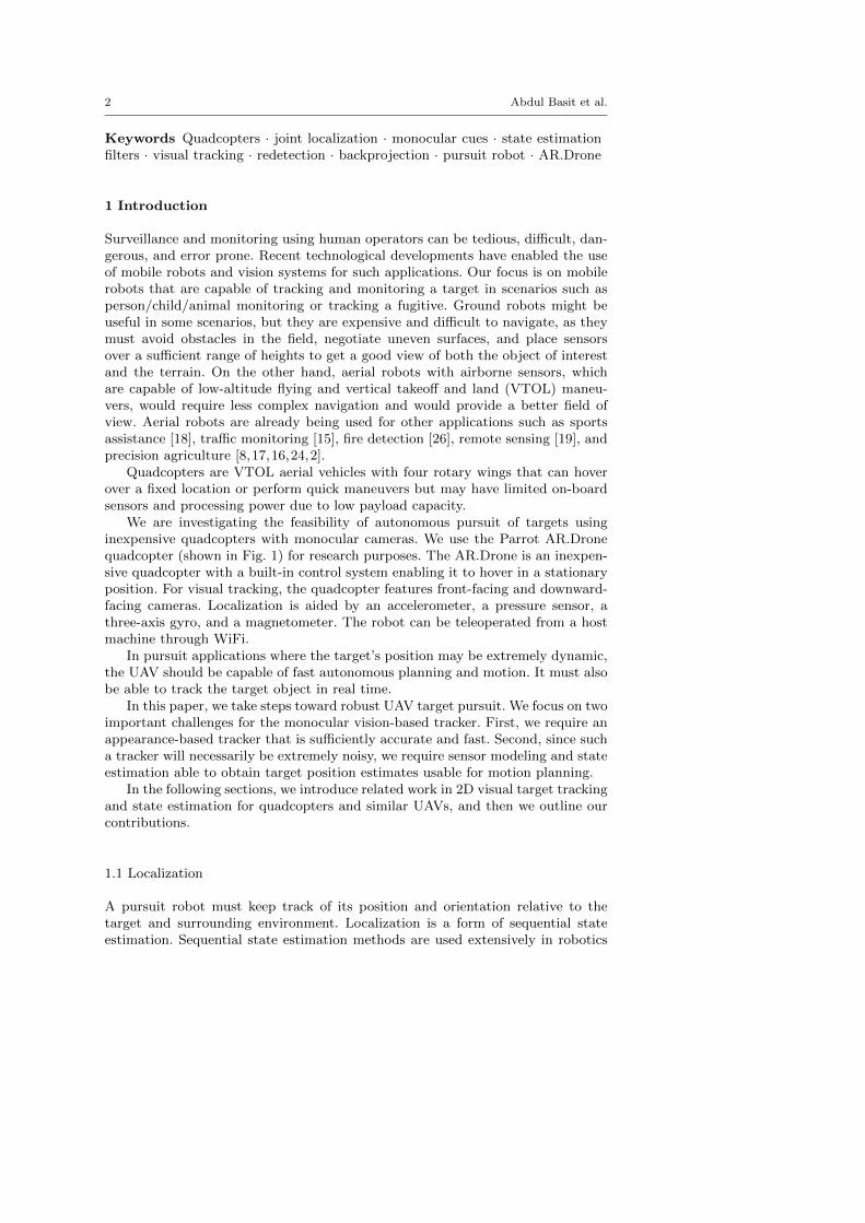
We are investigating the feasibility of autonomous pursuit of targets usinginexpensive quadcopters with monocular cameras. We use the Parrot AR.Dronequadcopter (shown in Fig. 1) for research purposes. The AR.Drone is an inexpen-sive quadcopter with a built-in control system enabling it to hover in a stationaryposition. For visual tracking, the quadcopter features front-facing and downward-facing cameras. Localization is aided by an accelerometer, a pressure sensor, athree-axis gyro, and a magnetometer. The robot can be teleoperated from a hostmachine through WiFi.

In pursuit applications where the target’s position may be extremely dynamic,the UAV should be capable of fast autonomous planning and motion. It must alsobe able to track the target object in real time.

In this paper, we take steps toward robust UAV target pursuit. We focus on twoimportant challenges for the monocular vision-based tracker. First, we require anappearance-based tracker that is sufficiently accurate and fast. Second, since sucha tracker will necessarily be extremely noisy, we require sensor modeling and stateestimation able to obtain target position estimates usable for motion planning.

In the following sections, we introduce related work in 2D visual target trackingand state estimation for quadcopters and similar UAVs, and then we outline ourcontributions.

1.1 Localization

A pursuit robot must keep track of its position and orientation relative to thetarget and surrounding environment. Localization is a form of sequential stateestimation. Sequential state estimation methods are used extensively in robotics

Joint Localization of Pursuit Quadcopters and Target Using Monocular Cues 3

and computer vision to solve problems such as SLAM, monocular SLAM [12],visual target tracking [25], and 3D reconstruction. Methods include Kalman filters,particle filters [29], and grid-based methods. The most widely used filtering methodthat supports non-linear state estimation models is the extended Kalman filter [34].

EKF models are fast and effective in any application in which the posteriorstate estimate is accurately represented by a Gaussian and the non-linearities inthe system and sensor are moderate. EKFs have been used by several researchersto improve the performance of visual tracking methods [31,14,20].

Finding the position of a target relative to a UAV using a monocular camerarequires extraction of depth cues from the 2D image. Monocular depth cues areextremely noisy, so relying purely on the 2D image to obtain 3D positions withdepths would introduce a great deal of error. One way to improve the noisy sensorreadings we would get from a 2D visual tracker is to filter sensor based estimateswith a sequential state estimator.

In a previous paper [4], we propose a state estimation model based on theEKF for pursuit by SUGVs (Small Unmanned Ground Vehicles) to improve theaccuracy of the estimated trajectory of both the pursuit robot and the target. Theproposed method fuses robot kinematics and target dynamics to obtain superiorrobot and target trajectory estimates.

In this paper, based on our previous work, we propose a joint localization modelthat fuses quadcopter kinematics with target dynamics to improve the relativetrajectory estimates of both the quadcopter and the target.

1.2 2D object tracking

The major methods for 2D image-based tracking use either feature matching, op-tical flow, or feature histograms. Feature matching algorithms such as SIFT [36],SURF [33], and shape matching algorithms such as contour matching [35] aretoo computationally expensive to be considered for real-time tracking by a smallUAV with modest compute resources. Optical flow methods [13] or [30] may bewithin reach in terms of speed, but they do not maintain an appearance model.Histogram-based trackers, on the other hand, are not only fast, but also maintainan appearance model that is potentially useful for recovering tracking after anocclusion or reappearance in the field of view.

The Sliding window is a general approach in computer vision to look for a targetobject in an image. The naive sliding window approach is however, a computa-tionally inefficient way to scan an image to search for a target. Porikli [28] proposean “integral histogram” method using integral images to speed up the process.Perreault and Hebert [27] compute histograms for median filtering efficiently bymaintaining separate column-wise histograms, and, as the sliding window movesright, first updating the relevant column histogram then adding and subtractingthe relevant column histograms to the histogram for the sliding window. Sizint-sev et al. [32] take a similar approach to obtain histograms over sliding windowsby efficiently updating the histogram using previously calculated histograms foroverlapping windows.

CAMSHIFT (Continuously Adaptive Mean Shift) [6,1] is a fast and robustfeature histogram tracking algorithm potentially useful for UAVs. The methodbegins with manual initialization from a target image patch. It then tracks the


Fig. 1 Quadcopter visual sensors and coordinate system. The AR.Drone quadcopter incorpo-rates a front-facing and downward-facing camera. Roll (γrt ) and pitch (βrt ) are used to controlforward-backward and left-right linear motions. Overall rotor speed is used to control upward-downward motion. Yaw control is used for change in orientation. The front-facing camera isuseful in applications such as tracking and surveillance. The downward camera is useful forinspecting buildings, crops, or a field.

region using a combination of color histograms, the basic mean-shift algorithm[10,11], and an adaptive region-sizing step. It is scale and orientation invariant.Unfortunately, since the method performs a search for a local peak in the globalbackprojection, it is easily distracted by background objects with similar color dis-tributions. In this paper, we incorporate an adaptive histogram similarity thresholdwith CAMSHIFT to help avoid tracking false targets. We also use this adaptivesimilarity threshold with a backprojection technique to recover the target objectand reinitialize the CAMSHIFT visual tracker after an occlusion.

1.3 Monocular visual tracking by UAVs

Bi and Duan [5] implement a visual tracking algorithm using a low-cost quad-copter. The target is a colored landing platform that is moved manually on a cart.The quadcopter is controlled by a host machine that processes the video streamand tracks the landing platform. The host machine calculates the current positionof the landing platform by using the centroid of image moments calculated fora binary image that is obtained after thresholding the green channel of the RGBimage. The authors use independent controllers for pitch and roll that receive feed-back from the visual tracker. The feedback input to the controllers at each frameis the current positioning error.

Kim and Shim [21] present a visual tracker and demonstrate its capabilitiesand usage on a tablet computer with the AR.Drone. The method uses color andimage moments for the visual tracker.


All of the object tracking and navigation algorithms proposed thus for low costUAVs use color and image moments. None of this work has demonstrated model-based object tracking that is sufficiently fast and accurate for real time control ofa UAV.

1.4 Contributions

In this paper, we propose a novel joint purser and target localization model specifi-cally for the AR.Drone that reduces position estimation error caused by monocularsensor measurements. The model maintains an estimate of the state of the target,assuming a simple linear dynamical model, as well as an estimate of the AR.Dronerobot’s state, assuming standard quadcopter robot kinematics [7].

We additionally propose a target tracking method suitable for quadcopters thatefficiently handles both visual detection and tracking in real time. We performtarget redetection when the target is occluded or leaves the field of view. Wesuspend tracking based on an adaptive histogram threshold. Once the object isreacquired in a redetection phase, we apply CAMSHIFT to confirm the redetectedobject. After CAMSHIFT validation, we reinitialize the tracker.

We thus fuse information from 2D visual tracking and the UAV’s odome-try measurements with knowledge of the AR.Drone’s kinematics in an extendedKalman filter to obtain superior state estimation. The filter significantly improvesestimation accuracy compared to standard sensor-based position estimates as wellas compared to localization models not incorporating pursuit robot kinematics.

In an empirical evaluation, we show, on real-world videos, that the proposedmethod is a robust approach to target tracking and redetection during pursuitthat is accurate, is successful at reinitialization, has very low false positive rates,and runs in real time.

2 System Design

In this section, we introduce the AR.Drone’s hardware (sensors and actuators),provide details of the pursuer-pursuit-target localization method for the AR.Drone,and finally describe the visual target tracking method.

2.1 Quadcopter overview

The AR.Drone has a carbon fiber support structure and a plastic body with re-movable hulls optimized for indoor and outdoor flight. The rotors are propelled byhigh-efficiency brushless DC motors and control circuitry. The drone is equippedwith one frontal and one bottom facing camera. The control board of the AR.Droneconsists of a 1-GHz ARM-Cortex-A8 32-bit processor with an 800 MHz digital sig-nal processor and 2GB RAM. The user can control the quadcopter’s roll, pitch,yaw, and vertical speed through a host machine over a WiFi link. The functionof the control board is to convert user navigation commands into motor com-mands and to adjust the motor speeds to stabilize the drone at the required pose.Fig. 2 shows how the drone communicates with the host machine. We use the video


Fig. 2 System architecture and data flow. The base station receives sensor data (images andodometry) at the given rates and latencies. The frequency of the odometry data (200 Hz)is high compared to the image transfer rate (18 fps), so it is straightforward to accumulateodometry data between images and perform a model update with the arrival of each image.

stream from the frontal camera as the main sensor for localization. The camera hasa frame rate of approximately 18 fps. Estimated roll, pitch, yaw, vertical speed,and velocity in the x-y plane are estimated from the onboard accelerometer, apressure sensor, a three-axis gyro, and a magnetometer. The estimated data aresent to the host at 200 Hz.

2.2 Mathematical model and algorithmic flow

In this section, we detail the joint localization method for the quadcopter purserand target. Joint localization incorporates both target dynamics and drone kine-matics to correct the sensor-based measurements of the target’s and purser’s state.As the main target state measurement sensor, we use the AR.Drone’s front-facingmonocular camera.

The tracking algorithm’s flow is shown in Fig. 3. The monocular 2D visualtracker tracks the target as long as it is in the field of view. The monocular visualtracker returns a 2D tracking window indicating the target’s size and positionin the image. To transform 2D measurements into 3D, we take a ray from thecamera center through the image plane at the center of the 2D target region andcalculate the depth of the target along that ray using the assumed target height inan absolute frame. Meanwhile, we acquire AR.Drone odometry data in the form,at time t, of (γrt , β

rt , α

rt , h

rt , x

rt , y

rt , z

rt ), where (γrt , β

rt , α

rt ) describes the roll, pitch

and yaw of the quadcopter, hrt is the measured altitude, and (xrt , yrt , z

rt ) is the


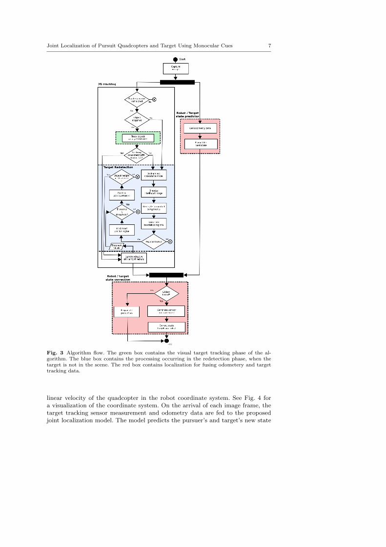
Fig. 3 Algorithm flow. The green box contains the visual target tracking phase of the al-gorithm. The blue box contains the processing occurring in the redetection phase, when thetarget is not in the scene. The red box contains localization for fusing odometery and targettracking data.

linear velocity of the quadcopter in the robot coordinate system. See Fig. 4 fora visualization of the coordinate system. On the arrival of each image frame, thetarget tracking sensor measurement and odometry data are fed to the proposedjoint localization model. The model predicts the pursuer’s and target’s new state


based on the previous state and corrects (updates) the estimate based on thenewly acquired sensor measurement. If the target is occluded or leaves the camerafield of view, we stop 2D tracking and state correction, and we run a redetectionalgorithm until the target reappears, at which time we restart the normal flow ofthe algorithm.

We briefly outline the visual tracking method below and provide more detailson the 3D state estimate model for the AR.Drone in the next section. Refer toBasit et al. [4] for more details on the 2D tracking algorithm, which proceeds asfollows:

1. Initialize CAMSHIFT with initial image I0 and bounding box (xc, yc, w, h).2. Continue CAMSHIFT tracking, updating adaptive histogram threshold.3. Suspend tracking when similarity between region returned by the tracker and

appearance model is too low.4. Run redetection.5. Suspend redectection when candidate target most similar to the appearance

model is similar and large enough.6. Run CAMSHIFT to confirm redetected region. If confirmed, reinitialize track-

ing; otherwise, return to redetection.

2.3 Joint Estimation of AR.Drone and Target State

In this section we describe the proposed model for obtaining smooth pursuer andtarget trajectories in the 3D world coordinate frame.

2.3.1 System state

The system state expresses the UAV’s position and the target’s position and ve-locity in the world coordinate frame. We define the system state at time t tobe

xt = [xt, yt, zt, xt, yt, zt, xrt , y

rt , z

rt , γ

rt , β

rt , α

rt ]

T, (1)

where (xt, yt, zt) is the target’s position, (xt, yt, zt) is the target’s velocity,(xrt , y

rt , z

rt ) is the pursuer’s position, and (γrt , β

rt , α

rt ) is the pursuer’s 3D orientation

(roll, pitch and, yaw) respectively. The positions and orientations are expressed inthe world coordinate frame. The state transition model is defined as

xt+1 = f(xt,ut) + νt, (2)

where νt ∼ N (0, Qt). f(xt,ut) has two components. The first component mod-els the AR.Drone’s kinematics, assuming constant linear and angular velocity overshort time periods (acceleration is modeled as noise). The second component isa first order linear dynamical system for the target’s motion. We describe eachcomponent in turn. The odometry control vector is

ut =[δγrt δβ

rt δα

rt δh

rt

]T, (3)

defining the change in the roll (γrt ), pitch (βrt ), yaw (αrt ), and altitude (hrt ) ofthe quadcopter at time t.


Fig. 4 Bird’s-eye view of quadcopter motion in 3D world coordinate frame. The motiondepends on changes of roll, pitch and altitude controls, that in turn produce 3D linear andangular motion. Linear velocity measurements (xrt , y

rt , z

rt ) are provided by three sensors. The

yaw (αrt ) angle is used to change the orientation of the quadcopter.

The state transition for the AR.Drone is then assumed to be

xrt+1 = xrt + (xrt cosαrt − yrt sinαrt ) ·∆tyrt+1 = yrt + (xrt sinαrt + yrt cosαrt ) ·∆tzrt+1 = zrt + δhrt

γrt+1 = γrt + δγrt

βrt+1 = βrt + δβrt

αrt+1 = αrt + δαrt , (4)

where (xrt , yrt ) is the linear velocity of the quadcopter in the (x,y) plane. This

velocity depends on the quadcopter’s roll and pitch in the world coordinate frame.See Fig. 5. We define the dynamics

xrt+1 = C1βrt

yrt+1 = C2γrt

(5)

To transform the linear velocities from the UAV frame to the world coordinateframe, we have

vwt = Rtvrt , (6)

where vrt is simply

vrt =[xrt y

rt z

rt

]T(7)

and Rt is

Rt =

cαrtcβr

tcαr

tsβr

tsγr

t− sαr

tcγr

tcαr

tsβr

tcγr

t+ sαr

tsγr

t

sαrtcβr

tsαr

tsβr

tsγr

t+ cαr

tcγr

tsαr

tsβr

tcγr

t− cαr

tsγr

t

−sβrt

cβrtsγr

tcβr

tcγr

t

,


-20

0

20

40

60

80

100

120

140

160

0 200 400 600 800

Mea

sure

d o

dom

etry

time t

Velocity control by pitch angle

Velocity (vx)Pitch

(a)

-15

-10

-5

0

5

10

15

20

0 200 400 600 800

Mea

sure

d o

dom

etry

time t

Velocity control by pitch angle

Velocity (vx)Pitch

(b)

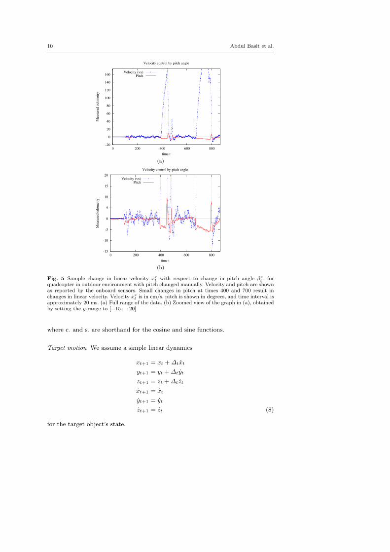
Fig. 5 Sample change in linear velocity xrt with respect to change in pitch angle βrt , forquadcopter in outdoor environment with pitch changed manually. Velocity and pitch are shownas reported by the onboard sensors. Small changes in pitch at times 400 and 700 result inchanges in linear velocity. Velocity xrt is in cm/s, pitch is shown in degrees, and time interval isapproximately 20 ms. (a) Full range of the data. (b) Zoomed view of the graph in (a), obtainedby setting the y-range to [−15 · · · 20].

where c· and s· are shorthand for the cosine and sine functions.

Target motion We assume a simple linear dynamics

xt+1 = xt +∆txt

yt+1 = yt +∆tyt

zt+1 = zt +∆tzt

xt+1 = xt

yt+1 = yt

zt+1 = zt (8)

for the target object’s state.


Linearization Since f(xt,ut) is nonlinear and we will be using an extended Kalmanfilter, we must approximate the system described in Eq. 2 by linearizing aroundan arbitrary point xt. We write

f(xt,ut) ≈ f(xt,ut) + Jft(xt − xt), (9)

where Jft is the Jacobian

Jft =

[∂f(xt,ut)

∂xt

](10)

evaluated at xt. We omit the detailed Jacobian calculations.

2.3.2 Sensor model

We assume the quadcopter’s target tracking camera is mounted in a fixed positionnear the UAV’s center of rotation with roll (rotation around the principal axis)close to 0. We also incorporate a 2D visual tracking algorithm capable of producingan estimate of the 2D position of the object’s projection into the image plane attime t. We assume the operator initially defines the target object to pursue byspecifying a bounding box around it in the first frame. We use visual trackerbased on CAMSHIFT to track the object from frame to frame.

The measurement from the algorithm is thus simply a bounding box:

zt =[ut, vt, w

imgt , himgt

]T, (11)

where (ut, vt) is the center and wimgt and himgt are the width and height of thebounding box in the image. We model the sensor with a function h(·) mappingthe system state xt to the corresponding sensor measurement

zt = h(xt) + ζt, (12)

with ζ ∼ N (0, St).For a pinhole camera with focal length f and principal point (cx, cy), ignoring

the negligible in-plane rotation of the cylindrical object, we can write the target’scenter (ut, vt) and size (wimgt , himgt ) as

ut = (fxcamt + cx)/zcamt

vt = (fycamt + cy)/zcamt

wimgt = fw0/zcamt

himgt = fh0/zcamt , (13)

where (h0, w0) is the assumed target’s height and width, xcamt = (xcamt , ycamt , zcamt , 1)T

is the homogeneous representation of the center of the target in the camera coor-dinate system, calculated as

xcamt = TW/Ct

xtytzt1

, (14)


where the transformation TW/Ct is defined as

TW/Ct = T

R/CTW/Rt , (15)

where TW/Rt is the rigid transformation from the world coordinate system to the

robot coordinate at time t, and TR/C is the (fixed) transformation from the robotcoordinate system to the camera coordinate system. Expressing the AR.Droneorientation by a rotation matrix R

T

t at time t, we can write the transformationmatrix TW/R

TW/Rt =

[R

T

t −RT

t xrt0

T1

], (16)

where xrt =[xrt y

rt z

rt

].

As with the transition model, to linearize h(xt) around an arbitrary point xt,we require the Jacobian

Jht=

[∂h(xt)

∂xt

]. (17)

evaluated at an arbitrary point xt.

2.3.3 Initialization

We require an a-priori state vector x0 to initialize the system. As explained before,we assume that the quadcopter is at the origin of the world coordinate system or analternative initial position of the robot is given. We do not assume any knowledgeof the target’s initial trajectory. We can therefore treat the user-provided initialtarget bounding box as a first sensor measurement z0 and initialing the system as

x0 = [x0, y0, z0, 0, 0, 0, 0, 0, 0, 0, 0, 0]T

= hinv(z0). (18)

To obtain (x0, y0, z0), we first calculate an initial target position in the camera-coordinate frame xcam0 then, noting that the robot frame at time 0 is also theworld frame, we can map to the world coordinate frame by

x0y0z01

=(TR/C

)−1

xcam0

ycam0

zcam0

1

. (19)

Inspecting the system in Eq. 13, we can find xcam0 and ycam0 given ut and vt if zcam0

is known. We can obtain zcam0 from wimg0 or himg0 . We use zimg0 = f · h/himg0 , onthe assumption that the user-specified bounding box is more accurate verticallythan horizontally.


2.3.4 Noise parameters

The sensor noise is given by the matrix St. We assume that the measurement noisefor both the bounding box center and the bounding box size are a fraction of thetarget’s width and height in the image:

St = λ2

(wimgt )2 0 0 0

0 (himgt )2 0 0

0 0 (wimgt )2 0

0 0 0 (himgt )2

. (20)

We use λ = 0.1 in our simulation, corresponding to 10% of the width and height ofthe target’s 2D bounding box in the image, determined through a series of exper-iments with the CAMSHIFT visual tracker in real environments. For the initialstate error denoted by P0, we propagate the measurement error for z0 throughhinv(z0) and take into account the initial uncertainty about the target’s velocity:

P0 = JhinvS0Jhinv + diag(0, 0, 0, η, η, η, 0, 0, 0, 0, 0, 0). (21)

η is a constant and Jhinv is the Jacobian of hinv(·) evaluated at z0.We assume that the state transition noise covariance Qt is diagonal for simplic-

ity. We tie the covariance Qt to the target linear velocities (xt, yt, zt), AR.Dronelinear velocities (xrt , y

rt , z

rt ) and orientation (γrt , β

rt , α

rt ) odometry reading. We let[

vtst

]=

[ √x2t + y2t + z2t√

(γrt )2 + (βrt )2 + (δαrt )2

]. (22)

We let the entries of Qt corresponding to the target position be ∆2t (ρ1v

2t + ρ2)

and the entries of Qt corresponding to the target velocity be ∆2t (ρ3v

2t +ρ4). We let

the entries of Qt corresponding to the AR.Drone’s position be ∆2t (ρ5s

2t + ρ6), and

we let the entries of Qt corresponding to the robot’s orientation be ∆2t (ρ7s

2t + ρ8).

This noise distribution is overly simplistic and may ignore some factors, but it issufficient for the experiments reported in this paper. In total, there are nine freeparameters (η, ρ1, ρ2, · · · , ρ8) that must be determined through hand tuning orcalibration. In our simulation, we find optimal free parameters free using gradientdescent.

2.3.5 Update algorithm

Given all the preliminaries specified in the previous sections, the update algo-rithm is just the standard extended Kalman filter, with modification to handlecases where the color region tracker fails due to occlusions or the target leavingthe field of view. When no sensor measurement zt is available, we simply predictthe system state and allow diffusion of the state covariance without sensor mea-surement correction. When we do have a sensor measurement but the estimatedstate is far from the predicted state, we reset the filter, using the existing robotposition and orientation but fixing the relative target state to that predicted byhinv(zt) and fixing the elements of Pt by propagating the sensor measurementerror for zt through hinv(zt) as previously explained in Section 2.3.4. Here is asummary of the algorithm:


1. Input z0.2. Calculate x0 and P0.3. For t = 1, . . . , T , do

(a) predict x−t = f(xt−1,ut−1),

(b) calculate Jft and Qt,(c) predict P−t = JftPt−1J

T

ft + Qt.(d) If zt is unavailable,

i. let xt = x−t ,

ii. let Pt = P−t .(e) Otherwise

i. calculate Jht, St, and Kalman gain

Kt = P−t JT

ht(Jht

P−t JT

ht+ St)

−1,

ii. estimate xt = x−t + Kt(zt − ht(x

−t )),

iii. update the error estimate Pt = (I− KtJht)P−t .

(f) If ‖xt − x−t ‖ > σ, reset the filter.

3 Experimental setup

We tested the performance and efficacy of the proposed method by carrying outexperiments, not only on synthetic data, but also in real-world scenarios. Beforedeploying to the real AR.Drone, we performed a simulation to test model correct-ness and effectiveness. We then carried out real-world experiments in both indoorand outdoor environments. We compare the proposed joint estimation model withtwo baselines: 1) relative localization without any filtering, and 2) relative localiza-tion with Kalman filter-based sensor correction but no joint estimation of purserand target state. We analyze the data quantitatively for indoor and qualitativelyfor outdoor environments.

For the simulation experiment, we generated pose data without any noise bothfor the AR.Drone and target object. The data consist of the target’s simulatedposition with appropriate velocity and simulated AR.Drone’s odometry (orien-tation and linear velocities). We used these as ideal ground truth trajectories.We then produced noisy simulated odometry readings. In order to generate cor-responding noisy trajectories, we added noise to the AR.Drone odometry datathen accumulated the data to obtain a trajectory. We also added noise to the 2Dtarget bounding box. Direct calculation of pursuer and target positions from thenoisy odometry and noisy target bounding boxes gives us baseline method 1, i.e.,sensor-only relative localization without filtering. We simulated a camera generat-ing 640×480 images at 20 fps with a focal length of 550 pixels (horizontal field ofview 60◦).

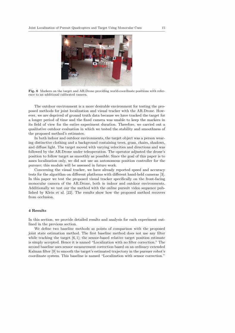
For the real-world experiments, we performed quantitative evaluation in indoorenvironments, where we acquired ground truth data for the target and purserusing circular markers pasted on the two objects. The circular markers were ofa known diameter. We use a fixed, calibrated camera to track the markers inorder to estimate, as accurately as possible, real-world ground truth for both thetarget and the AR.Drone using Krajnık and Nitsche’s method [23]. See Fig. 6 fora photo of experiment setting. We use these ground truth data for computing rootmean square error (RMSE). We also tested the proposed visual tracking with theAR.Drone’s front facing monocular camera in this indoor environment.


Fig. 6 Markers on the target and AR.Drone providing world-coordinate positions with refer-ence to an additional calibrated camera.

The outdoor environment is a more desirable environment for testing the pro-posed methods for joint localization and visual tracker with the AR.Drone. How-ever, we are deprived of ground truth data because we have tracked the target fora longer period of time and the fixed camera was unable to keep the markers inits field of view for the entire experiment duration. Therefore, we carried out aqualitative outdoor evaluation in which we tested the stability and smoothness ofthe proposed method’s estimates.

In both indoor and outdoor environments, the target object was a person wear-ing distinctive clothing and a background containing trees, grass, chairs, shadows,and diffuse light. The target moved with varying velocities and directions and wasfollowed by the AR.Drone under teleoperation. The operator adjusted the drone’sposition to follow target as smoothly as possible. Since the goal of this paper is toasses localization only, we did not use an autonomous position controller for thepursuer; this module will be assessed in future work.

Concerning the visual tracker, we have already reported speed and accuracytests for the algorithm on different platforms with different hand-held cameras [3].In this paper we test the proposed visual tracker specifically on the front-facingmonocular camera of the AR.Drone, both in indoor and outdoor environments.Additionally we test our the method with the online pursuit video sequence pub-lished by Klein et al. [22]. The results show how the proposed method recoversfrom occlusion.

4 Results

In this section, we provide detailed results and analysis for each experiment out-lined in the previous section.

We define two baseline methods as points of comparison with the proposedjoint state estimation method. The first baseline method does not use any filterwhile tracking the target [6,1]; the sensor-based relative target position estimateis simply accepted. Hence it is named “Localization with no filter correction.” Thesecond baseline uses sensor measurement correction based on an ordinary extendedKalman filter [9] to smooth the target’s estimated trajectory in the pursuer robot’scoordinate system. This baseline is named “Localization with sensor correction.”


-0.2

0

0.2

0.4

0.6

0.8

1

1.2

1.4

0 20 40 60 80 100

Rel

ativ

e ta

rget

posi

tion e

rror

% odometry error

Estimated joint target position error on various level of odometry noise

No filter correctionLocalization based on sensor correction

Joint localization method

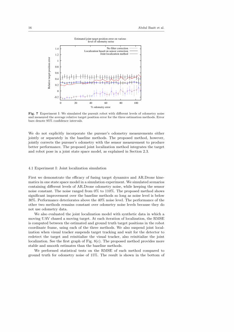
Fig. 7 Experiment I: We simulated the pursuit robot with different levels of odometry noiseand measured the average relative target position error for the three estimation methods. Errorbars denote 95% confidence intervals.

We do not explicitly incorporate the pursuer’s odometry measurements eitherjointly or separately in the baseline methods. The proposed method, however,jointly corrects the pursuer’s odometry with the sensor measurement to producebetter performance. The proposed joint localization method integrates the targetand robot pose in a joint state space model, as explained in Section 2.3.

4.1 Experiment I: Joint localization simulation

First we demonstrate the efficacy of fusing target dynamics and AR.Drone kine-matics in one state space model in a simulation experiment. We simulated scenarioscontaining different levels of AR.Drone odometry noise, while keeping the sensornoise constant. The noise ranged from 0% to 110%. The proposed method showssignificant improvement over the baseline methods so long as noise level is below30%. Performance deteriorates above the 40% noise level. The performance of theother two methods remains constant over odometry noise levels because they donot use odometry data.

We also evaluated the joint localization model with synthetic data in which amoving UAV chased a moving target. At each iteration of localization, the RMSEis computed between the estimated and ground truth target positions in the robotcoordinate frame, using each of the three methods. We also suspend joint local-ization when visual tracker suspends target tracking and wait for the detector toredetect the target and reinitialize the visual tracker, also reinitialize the jointlocalization. See the first graph of Fig. 8(c). The proposed method provides morestable and smooth estimates than the baseline methods.

We performed statistical tests on the RMSE of each method compared toground truth for odometry noise of 15%. The result is shown in the bottom of


Baseline sensor-based localization with no filteringBaseline relative localization with sensor correction

Joint localization

Rela

tiv

e l

ocali

zati

on

err

or

0

1

2

3

4

50 100 150 200 250 300 350 400 450 500

0

1

2

3

4

50 100 150 200 250 300 350

0

0.4

0.8

20 40 60 80 100 120

Odometry sample # (20 samples/s)

Av

erag

e re

lati

ve

loca

liza

tio

n e

rror

0

0.2

0.4

0.6

0.8

1

1

0

0.2

0.4

0.6

0.8

1

1.2

1.4

1 0

0.05

0.1

0.15

0.2

0.25

0.3

0.35

(a) indoor - large open room (b) indoor - corridor (c) simulation

Fig. 8 Experiment I and II: Quantitative evaluation with real world (indoor) and syntheticdata. First row shows relative target position root mean squared error (RMSE) of the tar-get in the robot coordinate frame. Second row reflects accumulated average error with 95%confidence interval. (a) Real world indoor experiment in closed hall. The proposed methodprovides smooth and stable estimates, 44% and 22% better than the baseline methods. (b)Indoor experiment in a corridor. RMSE is 56% and 28% lower than with the baseline methods(c) Simulation with synthetic data.The proposed method outperforms tracking method with-out model-based correction by 75% and outperforms the sensor-based correction method by27%.

Fig. 8(c). The proposed method outperforms the existing methods by 65% and25%.

4.2 Experiment II: Indoor joint localization

In Experiment II, we carried out indoor experiments with quantitative analysis.We used ground truth data for comparison between the proposed and existingmethods.

At every iteration of each algorithm, at time t, we transformed the targetposition (xt, yt, zt) to the AR.Drone coordinate reference frame. We calculatedroot mean squared error between each method’s estimate and ground truth. SeeFig. 8(a) and 8(b) top row. We collapse the results of multiple indoor runs intotwo cases, a large open room and a corridor.

The proposed method clearly obtains smoother and more stable estimates com-pared to the baseline methods. Although relative localization with sensor correc-tion produces better results when compared with localization with no filter, ourjoint localization method, fusing sensor measurements and odometry data, pro-duces additional improvement.

As with the simulation data, we computed the average root mean square errorover all runs. The results shown in the bottom row of Fig. 8(a) and 8(b). The


results show that the filtering methods help smooth the raw sensor measurements,but the proposed joint localization method outperforms not only the method withno filter but also relative localization with sensor correction. Joint localizationimproves relative target position estimation over both baseline methods.

4.3 Experiment III: Outdoor joint localization

As mentioned earlier, though quantitative analysis is not possible outdoors, wedid perform an outdoor experiment to ensure the practicality of the proposedapproach. We evaluated our method at several stages of the visual tracking andlocalization process. First we show results when the target is standing still andthe UAV is simply hovering. See Fig. 9(a). Next we show results when the targetis moving with variable velocity and the UAV is accelerating to catch up with thetarget. See Fig. 9(b). Finally, we show results when sensor noise increases due tochanges in background and lighting. See Fig. 9(c).

Refer to Fig. 9(a). The estimated X position varies between 5.5 and 7.5 meters,a range of 2 meters. Recall from Fig. 1 that the target’s position X is the distanceof the target from the AR.Drone in the forward direction. The proposed method’sestimated trajectory, shown in red, is smoother and has lower variance than thatof the other methods. The spikes in the trajectory reflect noisy variation in theestimated 2D bounding box’s size. The joint localization method infers smoothtransitions between neighboring intervals. The estimated Y position varies between0 and 0.4 meters. The variation is lower on this axis, reflecting lower noise in theestimated left-right position of the 2D bounding box. The proposed method againperforms better than the baseline methods. Finally, the estimated Z position variesbetween -0.5 and -1.2 meters. We observe more spikes or jerking movements onthis axis, generally caused by the UAV’s pitch control. The Z position estimatesare again smoother than for other baseline methods. Overall, the joint localizationmethod clearly performs better than the baseline methods.

Next, refer to Fig. 9(b). During this period, the target is moving away fromAR.Drone, which is attempting to catch up. The AR.Drone begins accelerating att = 200 and decelerating at t = 265. The estimated X position varies between 5.5and 8.0 meters. The large black-dotted spike indicates extreme sensor noise whenthe AR.Drone started decelerating. xrt is minimized when the pitch βrt = 0. Thesame spike can be observed in the Y target position in the robot coordinate frame.Here the noise varies between 0 and 0.6 meters. Clearly the proposed method issmoother and more stable along both the X and Y axis, even with the velocityvariation of the AR.Drone. Finally, the estimated Z position varies between -1 and0.5 meters. The change in Z at t = 213 is caused by the UAV’s forward pitch,causing it to move. When the AR.Drone decelerates, we obtain noise in sensorand odometry measurements, so we observe more variability between t = 270 andt = 295. The overall performance of joint localization is clearly better than theother methods.

Now we turn to Fig. 9(c). We observe an increased number of spikes in thetrajectories caused by error in the 2D bounding box estimates. This noise resultsin unstable prediction, challenging the proposed joint localization method. Theestimated position of the target varies between 5.4 and 10 meters, the estimatedY position varies between 0 and 0.8 meters, and the estimated Z position varies


Baseline sensor-based localization with no filteringBaseline relative localization with sensor correction

Joint localization

5.6

6.4

7.2

X

5.6

6.4

7.2

8

8.8

5.6

6.4

7.2

8

8.8

9.6

0

0.2

0.4

Y

0

0.2

0.4

0.6

0

0.2

0.4

0.6

0.8

-0.5

-0.25

20 40 60 80 100 120 140 160 180

Z

-1

-0.5

0

0.5

180 200 220 240 260 280 300

-1.95

-1.3

-0.65

0

300 350 400 450 500 550

(a) (b) (c)

Fig. 9 Experiment III: outdoor qualitative evaluation. Stability and smoothness of estimatedtarget position (X,Y, Z) in the robot coordinate frame, where X is forward, Y is left, and Zis upward. Each subplot’s ordinate shows the target’s position on one axis in meters, whilethe abcissa shows time varying between 1 and 550 over all three subfigures. (a) Target isstationary and UAV is simply hovering. The peaks at t = 130 in Y and Z are generated whenUAV moves to adjust its position relative to the target. (b) Target is moving and UAV isaccelerating at t = 210 and decelerating at t = 260 to catch up with the target. (c) Visualsensor noise increases because of lighting and clutter in the background. Higher noise on Xaxis shows higher variance due to 2D bounding box error.

between -1.5 and 0.6 meters. The proposed method performs better than the othertwo methods in terms of stability and smoothness.

4.4 Experiment IV: Visual tracking

We tested the visual tracker in both indoor and outdoor environments. In Fig. 10,the first column shows outdoor results with our AR.Drone. The second columnshows results of processing an online pursuit video sequence by Klein et al. [22],and the last two columns show indoor results with our AR.Drone in a large openroom and corridor.

Based on the first frame of each video (R1 in Fig. 10), we initialized CAMSHIFTtracking by manually providing a bounding box for the human target in the scene.We then ran the proposed tracking, suspension, and redetection method to theend of each video.

During tracking, our method incrementally updated the mean µt and standarddeviation σt of the distance dt between the appearance model Hm and the trackedtarget’s color histogram Hr

t . In almost all cases, when the target left the scene,the distance dt exceeded the adaptive threshold, except for a few cases in whichthe redetection algorithm found a sufficiently similar object in the background.


R1: Frame beforetracking initialization

R2: Target leaves thescene

R3: Candidate regions(none are selected)

R4: Target returns tothe scene

R5: Candidate regions(target is selected)

R6: CAMSHIFTreinitialization

Fig. 10 Experiment IV: Visual tracker evaluation. The proposed method was tested in dif-ferent environments with different background and target objects. Each column shows imagesfrom a different video. Rows show results of each step of processing. Blue colored rows showprocessing when the target is not in the scene. Yellow colored rows show the same processingsteps when the target returns to the scene.

Rows R2 and R3 in Fig. 10 show example images acquired when the targetwas absent from the camera field of view. At this point in each video, CAMSHIFTtracking is suspended and the redetection algorithm is running, correctly reportingthe absence of the target from the field of view.

Rows R4 and R5 in Fig. 10 show example images acquired after the targethas returned to the field of view. The proposed method eventually successfullyidentifies the candidate region among the possible candidates. In the figure, theselected region is surrounded by a red rectangle.

In each of the four cases shown, CAMSHIFT is correctly reinitialized, as shownin row R6 of Fig. 10.

Over the four videos, the target was successfully tracked in 95.6% of the framesin which the target was in the scene, with false positives occurring in only 4.4%of the frames in which the target was not in the scene. The accuracy results on aper-video basis are summarized in Table 1.

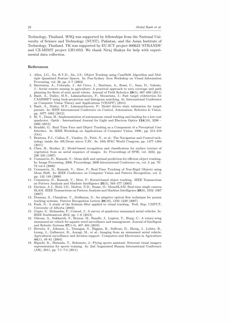
We tested the runtime performance of the system on two different hardwareconfigurations, a 2.26 GHz Intel Core i3 laptop running 32-bit Ubuntu Linux 11.10and a 1.6 GHz Intel Atom N280 single core netbook running 32-bit Lubuntu 11.10.The results are summarized in Table 2. Both redetection and tracking run at highframe rates, with the worst case of just over 10 fps for redetection on the Atom


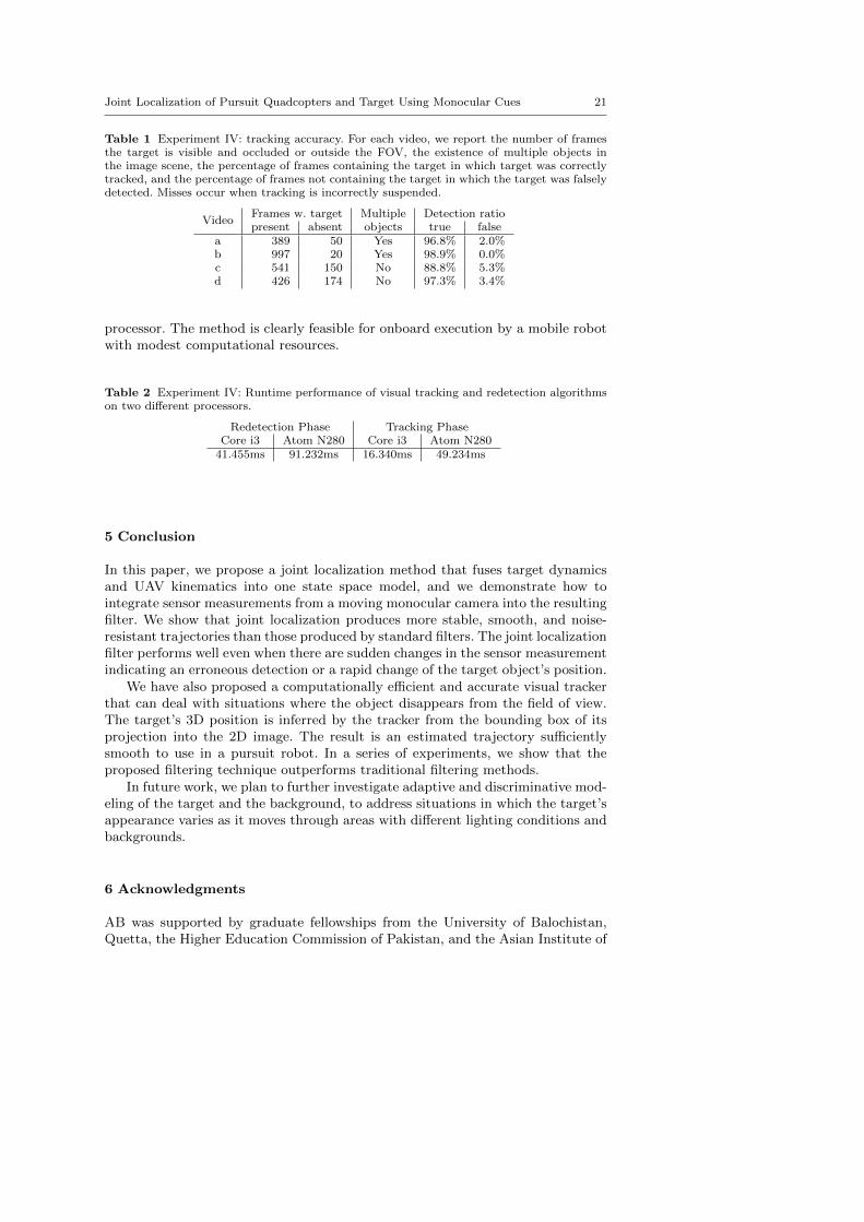
Table 1 Experiment IV: tracking accuracy. For each video, we report the number of framesthe target is visible and occluded or outside the FOV, the existence of multiple objects inthe image scene, the percentage of frames containing the target in which target was correctlytracked, and the percentage of frames not containing the target in which the target was falselydetected. Misses occur when tracking is incorrectly suspended.

VideoFrames w. target Multiple Detection ratiopresent absent objects true false

a 389 50 Yes 96.8% 2.0%b 997 20 Yes 98.9% 0.0%c 541 150 No 88.8% 5.3%d 426 174 No 97.3% 3.4%

processor. The method is clearly feasible for onboard execution by a mobile robotwith modest computational resources.

Table 2 Experiment IV: Runtime performance of visual tracking and redetection algorithmson two different processors.

Redetection Phase Tracking PhaseCore i3 Atom N280 Core i3 Atom N280

41.455ms 91.232ms 16.340ms 49.234ms

5 Conclusion

In this paper, we propose a joint localization method that fuses target dynamicsand UAV kinematics into one state space model, and we demonstrate how tointegrate sensor measurements from a moving monocular camera into the resultingfilter. We show that joint localization produces more stable, smooth, and noise-resistant trajectories than those produced by standard filters. The joint localizationfilter performs well even when there are sudden changes in the sensor measurementindicating an erroneous detection or a rapid change of the target object’s position.

We have also proposed a computationally efficient and accurate visual trackerthat can deal with situations where the object disappears from the field of view.The target’s 3D position is inferred by the tracker from the bounding box of itsprojection into the 2D image. The result is an estimated trajectory sufficientlysmooth to use in a pursuit robot. In a series of experiments, we show that theproposed filtering technique outperforms traditional filtering methods.

In future work, we plan to further investigate adaptive and discriminative mod-eling of the target and the background, to address situations in which the target’sappearance varies as it moves through areas with different lighting conditions andbackgrounds.

6 Acknowledgments

AB was supported by graduate fellowships from the University of Balochistan,Quetta, the Higher Education Commission of Pakistan, and the Asian Institute of


Technology, Thailand. WSQ was supported by fellowships from the National Uni-versity of Science and Technology (NUST), Pakistan, and the Asian Institute ofTechnology, Thailand. TK was supported by EU-ICT project 600623 ‘STRANDS’and CZ-MSMT project LH11053. We thank Niraj Shakya for help with experi-mental data collection.

References

1. Allen, J.G., Xu, R.Y.D., Jin, J.S.: Object Tracking using CamShift Algorithm and Mul-tiple Quantized Feature Spaces. In: Pan-Sydney Area Workshop on Visual InformationProcessing, vol. 36, pp. 3–7 (2004)

2. Barrientos, A., Colorado, J., del Cerro, J., Martinez, A., Rossi, C., Sanz, D., Valente,J.: Aerial remote sensing in agriculture: A practical approach to area coverage and pathplanning for fleets of mini aerial robots. Journal of Field Robotics 28(5), 667–689 (2011)

3. Basit, A., Dailey, M.N., Lakanacharoen, P., Moonrinta, J.: Fast target redetection forCAMSHIFT using back-projection and histogram matching. In: International Conferenceon Computer Vision Theory and Applications (VISAPP) (2014)

4. Basit, A., Dailey, M.N., Laksanacharoen, P.: Model driven state estimation for targetpursuit. In: IEEE International Conference on Control, Automation, Robotics & Vision,pp. 1077–1082 (2012)

5. Bi, Y., Duan, H.: Implementation of autonomous visual tracking and landing for a low-costquadrotor. Optik - International Journal for Light and Electron Optics 124(18), 3296 –3300 (2013)

6. Bradski, G.: Real Time Face and Object Tracking as a Component of a Perceptual UserInterface. In: IEEE Workshop on Applications of Computer Vision, 1998., pp. 214–219(Oct)

7. Bristeau, P.J., Callou, F., Vissiere, D., Petit, N., et al.: The Navigation and Control tech-nology inside the AR.Drone micro UAV. In: 18th IFAC World Congress, pp. 1477–1484(2011)

8. Chen, H., Houkes, Z.: Model-based recognition and classification for surface texture ofvegetation from an aerial sequence of images. In: Proceedings of SPIE, vol. 3222, pp.236–245 (1997)

9. Comaniciu, D., Ramesh, V.: Mean shift and optimal prediction for efficient object tracking.In: Image Processing, 2000. Proceedings. 2000 International Conference on, vol. 3, pp. 70–73 vol.3 (2000)

10. Comaniciu, D., Ramesh, V., Meer, P.: Real-Time Tracking of Non-Rigid Objects usingMean Shift. In: IEEE Conference on Computer Vision and Pattern Recognition, vol. 2,pp. 142–149 (2000)

11. Comaniciu, D., Ramesh, V., Meer, P.: Kernel-based object tracking. IEEE Transactionson Pattern Analysis and Machine Intelligence 25(5), 564–577 (2003)

12. Davison, A.J., Reid, I.D., Molton, N.D., Stasse, O.: MonoSLAM: Real-time single cameraSLAM. IEEE Transactions on Pattern Analysis and Machine Intelligence 29(6), 1052–1067(2007)

13. Denman, S., Chandran, V., Sridharan, S.: An adaptive optical flow technique for persontracking systems. Pattern Recognition Letters 28(10), 1232–1239 (2007)

14. Funk, N.: A study of the Kalman filter applied to visual tracking. Tech. Rep. CMPUT,University of Alberta (2003)

15. Gupte, S., Mohandas, P., Conrad, J.: A survey of quadrotor unmanned aerial vehicles. In:IEEE Southeastcon 2012, pp. 1–6 (2012)

16. Gktoan, A., Sukkarieh, S., Bryson, M., Randle, J., Lupton, T., Hung, C.: A rotary-wingunmanned air vehicle for aquatic weed surveillance and management. Journal of Intelligentand Robotic Systems 57(1-4), 467–484 (2010)

17. Herwitz, S., Johnson, L., Dunagan, S., Higgins, R., Sullivan, D., Zheng, J., Lobitz, B.,Leung, J., Gallmeyer, B., Aoyagi, M., et al.: Imaging from an unmanned aerial vehicle:Agricultural surveillance and decision support. Computers and Electronics in Agriculture44(1), 49–61 (2004)

18. Higuchi, K., Shimada, T., Rekimoto, J.: Flying sports assistant: External visual imageryrepresentation for sports training. In: 2nd Augmented Human International Conference(AH), 2011, pp. 7:1–7:4 (2011)


19. Jimenez-Berni, J.A., Zarco-Tejada, P.J., Suarez, L., Fereres, E.: Thermal and narrowbandmultispectral remote sensing for vegetation monitoring from an unmanned aerial vehicle.IEEE Transactions on Geoscience and Remote Sensing 47(3), 722–738 (2009)

20. Karavasilis, V., Nikou, C., Likas, A.: Visual tracking by adaptive Kalman filtering andmean shift. In: Artificial Intelligence: Theories, Models and Applications, pp. 153–162.Springer (2010)

21. Kim, J., Shim, D.: A vision-based target tracking control system of a quadrotor by usinga tablet computer. In: 2013 International Conference on Unmanned Aircraft Systems(ICUAS), pp. 1165–1172 (2013)

22. Klein, D.A., Schulz, D., Frintrop, S., Cremers, A.B.: Adaptive Real-Time Video-Trackingfor Arbitrary Objects. In: IEEE Int. Conf. on Intelligent Robots and Systems (IROS), pp.772–777 (2010)

23. Krajnık, T., Nitsche, M., et al.: External Localization System for Mobile Robotics. In:International Conference on Advanced Robotics. IEEE, Montevideo (2013)

24. Lan, Y., Thomson, S.J., Huang, Y., Hoffmann, W.C., Zhang, H.: Review: Current statusand future directions of precision aerial application for site-specific crop management inthe USA. Computer and Electronics in Agriculture 74(1), 34–38 (2010)

25. Lou, J., Yang, H., Hu, W.M., Tan, T.: Visual vehicle tracking using an improved EKF.In: Asian Conference of Computer Vision (ACCV), pp. 296–301 (2002)

26. Murphy, D.W., Cycon, J.: Applications for mini VTOL UAV for law enforcement. In:Enabling Technologies for Law Enforcement and Security, pp. 35–43. International Societyfor Optics and Photonics (1999)

27. Perreault, S., Hebert, P.: Median filtering in constant time. Image Processing, IEEETransactions on 16(9), 2389–2394 (2007)

28. Porikli, F.: Integral histogram: a fast way to extract histograms in cartesian spaces. In:Computer Vision and Pattern Recognition, 2005. CVPR 2005. IEEE Computer SocietyConference on, vol. 1, pp. 829–836 (2005)

29. Pupilli, M., Calway, A.: Real-time camera tracking using a particle filter. In: BritishMachine Vision Conference (2005)

30. Qureshi, W.S., Alvi, A.B.N.: Object Tracking Using Mach Filter and Optical Flow in Clut-tered Scenes and Variable Lighting Conditions. World Academy of Science, Engineeringand Technology 3(12), 642 – 645 (2009)

31. Shimin, F., Qing, G., Sheng, X., Fang, T.: Human tracking based on mean shift andKalman filter. In: Artificial Intelligence and Computational Intelligence, vol. 3, pp. 518–522 (2009)

32. Sizintsev, M., Derpanis, K., Hogue, A.: Histogram-based search: A comparative study. In:Computer Vision and Pattern Recognition, 2008. CVPR 2008. IEEE Conference on, pp.1–8 (2008)

33. Ta, D.N., Chen, W.C., Gelfand, N., Pulli, K.: Surftrac: Efficient tracking and continuousobject recognition using local feature descriptors. In: IEEE Conference on ComputerVision and Pattern Recognition., pp. 2937–2944 (2009)

34. Welch, G., Bishop, G.: An introduction to the kalman filter. Tech. rep., Chapel Hill, NC,USA (1995)

35. Yokoyama, M., Poggio, T.: A contour-based moving object detection and tracking. In:Visual Surveillance and Performance Evaluation of Tracking and Surveillance., pp. 271–276 (2005)

36. Zhou, H., Yuan, Y., Shi, C.: Object tracking using SIFT features and mean shift. ComputerVision and Image Understanding 113(3), 345–352 (2009)

joint localization of pursuit quadcopters and target using monocular cues

Documents