jako199811920205116.pdf - korea science

16

Simulation and Experiment of Distorted LFM Signals in Shallow Water Environment

* Young-Nam Na, *Mun-Sub Jumg, *Tae-Bo Shim, and **Chun-Duck Kim

Abstract

This paper attempts to examine the characteristics of underwater acoustic signals distorted in shallow water environments.

Time signals are simulated using an acoustic model that employs the Fourier synthesis scheme. An acoustic experiment

was conducted in the shallow sea near Pohang, Korea, where water depth is about 60 m. The environment in the simulat

ion is set up so that it approximates the experimental condition, which can be regarded as range-independent. The signal

is LFM (linear frequency modulated) type centered on one of the four frequencies 200, 400, 600 and 800 Hz, each being

swept up or down with the bandwidth of 100 Hz. To analyze the signal characteristics, the study introduces a spectrum

estimation scheme, pseudo Wigner-Ville distribution (PWVD). The simulated and measured signals suffer great interference

by the interactions of neighboring rays. Although there are constructive or destructive interference, the signals keep LFM

characteristics well. This is thought that only a few dominant rays of small loss contribute to the received signals in a

shallow water environment.

I. Introduction

Within the frame of linear acoustics there are fundam

entally two approaches to broadband modeling problem:

Fourier synthesis and direct computation [1]. The first is

to solve the pulse propagation via the frequency domain

by Fourier synthesis of CW results. This approach is at

tractive since it lequires li비e programming effort. That is,

any of the time-harmonic acoustic models can be linked

up with a pulse post-processor which numerically per

forms the Fourier synthesis based on a number of CW

calculations with the frequency band of interest. The

Fourier synthesis scheme is adopted to simulate the LFM

signals distorted in the environment. In the CW calculat

ion with each frequency an acoustic model based on the

parabolic equation (PE) is applied.

The LFM signals are chosen in this study because they

are relatively simple to be generated but ena비e to analyze

the distorted signals with ease. They are regarded to be

enough to accommodate the signal distortion caused by

the environment.

Few papers have been published to deal with the LFM

signals distorted by surrounding environment. Fieid et al.

[2] tried to simulate the signals distorted in the deep wa

ter environment using a time-domain PE (TDPE) model.

They considered relatively short range (5 km) compared

Agency for Defense Development, ChinhaePukyong National University, Pusan

Manuscript Received : March 23, 1998.

with the water depth (1.3 km). In these conditions the

traveling waves suffer one surface or/and bottom inter

action, yielding small distortion and loss.

This study assimes the environment to be shallow

water, and considers environmental variations in sound

speed profile and bottom property. The principal charac

teristics of shallow water propagation is that the sound

speed profile is downward decreasing or nearly constant

over depth, meaning that long-range propagation takes

place exclusively via bottom-interacting paths [1]. Hence,

the important paths are either refracted bottom-reflected

or surface-reflected-bottom-reflected. Typical shallow water

environments are fo나nd on the continental shelf for water

depth down to 200 m. The signals inevitably undergo di

stortions by the environment in which they propagate.

This paper is directed to examining the characteristics

of low-frequency LFM signals distorted in shallow water

environments. Section II describes the theories employed

in this study s나ch as Fourier synthesis and spectrum est

imation. Section III delivers the simulation res니ts with

LFM sign시s. The simulation is conducted by varying

sound speed profile, bottom property and source-receiver

range. Section IV presents the results with the exper

imental data. Section V gives the conclusions derived in

this study.

IL Theory

A. Fourier Synthesis of Frequency-Domain Solution

The inhomogeneous Helmholtz equation for a simple

Simulation and Experiment of Distorted LFM Signals in Shallow Water Environment 17

point source of strength S(⑦)at point r。is given by

[v2 +k2]P(ct), r) = S(tw) <5(r— r0), ⑴

where P is pressure field at frequency and position

r, and 8 is dirac delta function.

The solution of the time-dependent wave equation can

be obtained by an inverse Fourier transform of the frequ

ency-domain solution as

从七 2, t) = ~2^ J 8 S(0)」P(尸,n, a>) e,a}tda), (2)

where S((w) is the source spectrum and P( r, z, o)) is

the spatial transfer function. Here, it is assumed that the

environment could be described in a cylindrical coordin

ates (i.e., azimuthal variations are negligible). The main

computational effort is to find the transfer function at a

number of discrete frequencies within the frequency band

of interest. The calculation of the integral in Eq (2) is

then done by an fast Fourier transform (FFT) at each

spatial position (r, z) for which the pulse response is

desired.

Assuming that the source does not produce any signif

icant energy above a certain frequency , Eq (2) is

replaced by

p(r, z, /) = J S(a)) P( r, z, co) e}u3i do), (3)

where P( r, z, o)) represents a normalized transfer fun

ction. So, if P〈 r, n, co) represents pressure fi이d (trans

mission loss pressure), then S(a)) is the frequency spec

trum of the so나ice pressure at 1-m distance from the

source. To yield a real time series, it is necessary to in

clude the negative spectrum in the integration, or altema-

tiv이y to use the form

1 p "小啟力(匕瓦 £)= Re—* J。 S(a)) P( r, z, o)) eJa> d(o). (4)

The solution to the Helmholtz equation (1) is conjug

ate symmetric, i.e., P( r, z, — o)) = Rr, z,仞)，where

R ) means complex conjugate of R). In this paper, a

LFM signal is generated and its spectrum is imposed on

the Fourier synthesis as the source spectrum S((w)-

Eq. (4) is a continuous form to evaluate pressure field

at each time t. To be practically applicable, the pressure

field sho니d be expressed in discrete form from which

time signal can be obtained at each time step.

Let us assume that the response at a point (r, z) is

sought in a time window of length T, starting at some

time fmin. The time and freq나ency axes are then discret

ized as

t,= /min +，△£, /= 0,1,2, . . . (N~ 1),

g= I" 1= — (M2 —1),…(M2 — 1), (5)

with the samplings satisfying the relation

厶t厶(D = ■夸. (6)

Since T = N£\ t and △ = 2지 T, from the above rel

ation, the frequency resolution is given by

"으岩 = *• ⑺

Now the integral is replaced by a discrete sum. The

discretization in frequency introduces periodicity of T in

time with the result being a time-shifted sum of all the

periodic responses [3],

S 力(尸，Z, t* + nT)n 咸(8)

=国『寫_ I)S(S)[ R，次，饥)e '林纱]e'村

or by using the conjugate-symmetric property of the trans

fer function,

S 力(尸，z,n 咸⑼

=Re(又力)勺 J n、

with et — 1 (for /=0) or 2 (for I >0)-

The actual response in the selected time window [ ,

"nm + T ] then becomes

= aRe (客)饥""""J/ ”

一 " + 赤7、)，

” (10)

where the last term denotes the wrap-around or aliasing

from the periodic time windows. Main effort to obtain

time signals in Eq.(10) is devoted to computing pressure

field P( r, z, ty) in each spatial grid and frequency. This

is performed with an acoustic model based on the PE

scheme. In the simulation the center frequency is chosen

18 The Journal of the Acoustical Society of Korea, Vol. 17. No. 2E(1998)

as 200 Hz and the sampling frequency as 1024 Hz which

satisfies the Nyquist criterion.

B. Pseudo Wigner-Ville Distribution (PWVD)

We need a spectrum estimator to analyze the time

signal obtained by Eq. (10). The PWVD is mathemati

cally sophisticated approach capable of higher resolution

for a given length of data. This is a kind of time-frequ

ency distributions and is known to be suitable for

analyzing transient or other non-stationary phenomena. It

has been widely used in optics [4-6] and speech proces

sing [7, 8] mainly because it promises high resolution in

frequency and time.

The Wigner-Ville distribution (WVD) of signal s。)is

defined as [9]

uj) = j' $*(f — 을) s(t + 3)(H)

and discrete time form as [1이

W(.t, w) = 2 s s*(t-号)s(t 十号)c '5 . (12)r= - co Z 4

where s*(f) is the complex conjugate of signal $( t).

For a sampled signal s"](刀=0,1,2..........TV—1),

Eq. (12) changes into

W[l, k] =4 흐J s[l^n\s*[l-n\e '^nklN,N ”5 (13)

k=0, 1, 2..........N-l

where s[秫]=0 for m <0 and m > N— 1.

Basically, Eq. (13) has the form of the FFT and one

can utilize a FFT algorithm. However, Eq. (13) is rewrit

ten to know what periodicity the WVD has.

W[lt A+m(N/2)]

1 件누 _ -X쯔以+커쑝)—一卞 zJ s[ /+ n] s [ I— n] eIV n -• 0

1 ZV-1 一丿 4艾츠应= 前 4^ 5[ /+ n\ s* [ Z— h] e "。r섰께” (14)

=MA k]

since e ~ = 1 where m and n are integer.

From this illation it can be seen that the WVD has a

periodicity of 7V/2. Hence, even when the sampled data

s[ni\ satisfies the Nyquist criterion there wo니d be still

aliasing component in the WVD. A simple way to avoid

the aliasing is to introduce the analytic signal beforehand

[111-The analytic signal may be expressed by

s(t) = +

where is the Hilbert transform and obtained

convolving the imp나屁 response

as follows

(15)

h〈f) of 7r/2 phase shift

} = &(t) * h(f), (16)

where /心)=2 sin '(混/2)/混，t 丰 0

=0, f = Q.

Since the WVD has a periodicity of N/2, Eq. (13)

can be rewritten as follows

2gk^-0)] = 24t s[ (m + 〃)△ f]

q (17)

s*[(w-«) Me'*”"气

where △(〃= 찌(2N厶 t) and A t is the sampling interval.

In Eq. (17) the frequency resolution △⑦ is 1/4 of the

ordinary FFT, implying that the WDF guarantees four

times of frequency resolution.

To suppress the interference arising from cross terms,

a sliding window is applied in time-frequency domain.

The WVD with a window is usually called the PWVD or

smoothed WVD. The PWVD is obtained convolving the

WDF with Gaussian window function G as follows

W'H, 洞 = -응으으 '芸 W[f), q}G[p~ l, q- m\, (18)

where W" [ /, m\ is the PWVD, and

(心~]=任姦土^ exp [ -(令 +聂)].(19)

The signal s[ w] may be simulated pressure field or me

asured signal through sea experiment.

III. Sim비ated Signals

A. Input Data

To get distorted time signals, pressure fields satisfying

the wave equation should be computed first by using a

numerical model. The model is based on the PE scheme.

It requires mainly three kinds of environmental input

data : sound speed, density and attenuation. The time sign

als are obtained convolving source spectra with pressure

fields as described in the theory.

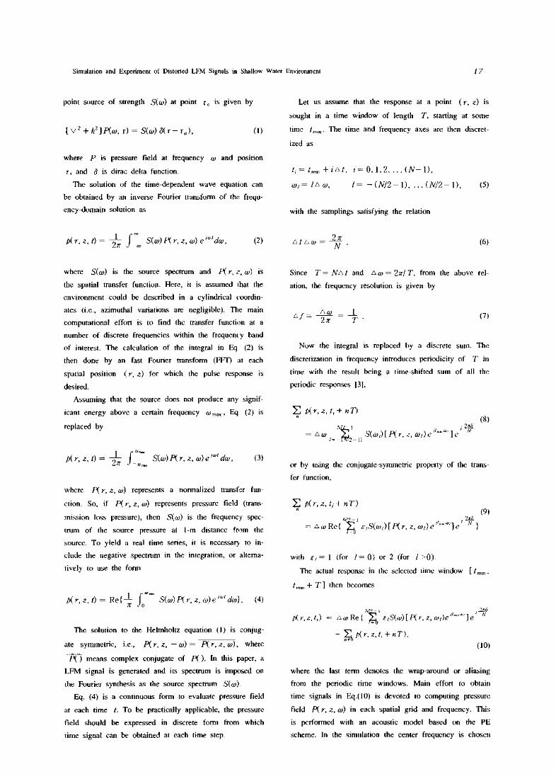
The environment, on which time signal simulation is

conducted, is a simple waveguide with pressure release

surface and penetrable fluid bottom (Fig. 1). The source


depth is 30 m and source-receiver range is one of 5, 10,

and 20 km. Two kinds of sound speed profile (SSP) are

assumed and they are typical in winter and summer in

shallow water. In the figure (Fig. lb) it can be seen that

the winter profile has actually one value of 1482 m/sec

over the water depth. That is, the water was mixed well

over the column. In winter, the surface water becomes

denser because it loses heat by the wind from northwest

that accelerates vertical mixing. The denser the surface

water becomes, the easier it descends down die water

column. On the other hand, the summer profile has neg

ative gradient over the water depth, which being particul

arly large between 20 and 30 m. In summer the surface

water is usually heated by the sun and thus it decreases

in density. Consequently, the water column becomes more

stable, meaning that it becomes more difficult to be mix

ed with the bottom water.

(a) geoacoustic data

source

•

zs 드 30 m

c„ = 1482 m/sec

p „ = 1000 kg/m360 m

\ cB1 = 1510 m/sec

\ pb= 1600 Kg/m3

\ - 0.5 dB/X .

\ cb2= 1600 m/sec

40 m

으트

Figural 1. Input data used for the time sign시 simulations.

The sediment parameters are shown in the figure including sound speed (cQ, density (pb), and attenuation

(ab). They are determined by referring to Miller and

Wolf [12]. The bottom properties are crucial to sound

wave propagation in shallow water because of the frequ

ent interactions of the waves with the bottom. The acou

stic model requires sound speed, attenuation coefficient,

density, and possibly shear speed. Most of these parame

ters, however, are not available at the desired site because

marine geology is rather complex and not well known.

Shear wave propagation in the bottom layer is not includ

ed based on the studies [13, 14] showing that the effect

of the low shear speed (below 300 m/sec) on sound wave

propagation in the water layer is weak and negligible.

B. Generation of LFM Signals

Once the pressure fields are computed by the model

they are convolved with source signals to give received

signals at each depth and range. The source signal is as

sumed to be projected from the source while received

ones to be distorted by the environment through which

the acoustic waves travel.

This study considers a LFM signal of which center fr

equency is 200 Hz and bandwidth is 100 Hz so that die

signal sweeps up or down in 150-250 Hz. The LFM

signal, 5(r), is generated by the following equation [15]

s(t) = sm[2jr(fot+ (20)

where f0 = center frequency (200 Hz), m = bandwidth

(100 Hz). For the upsweep signal the time goes from

—772 to T/2 and for the downsweep signal from T/2

to — T/2. The sampling frequency is 1024 Hz so that

1024 sequences are generated over a period of one second.

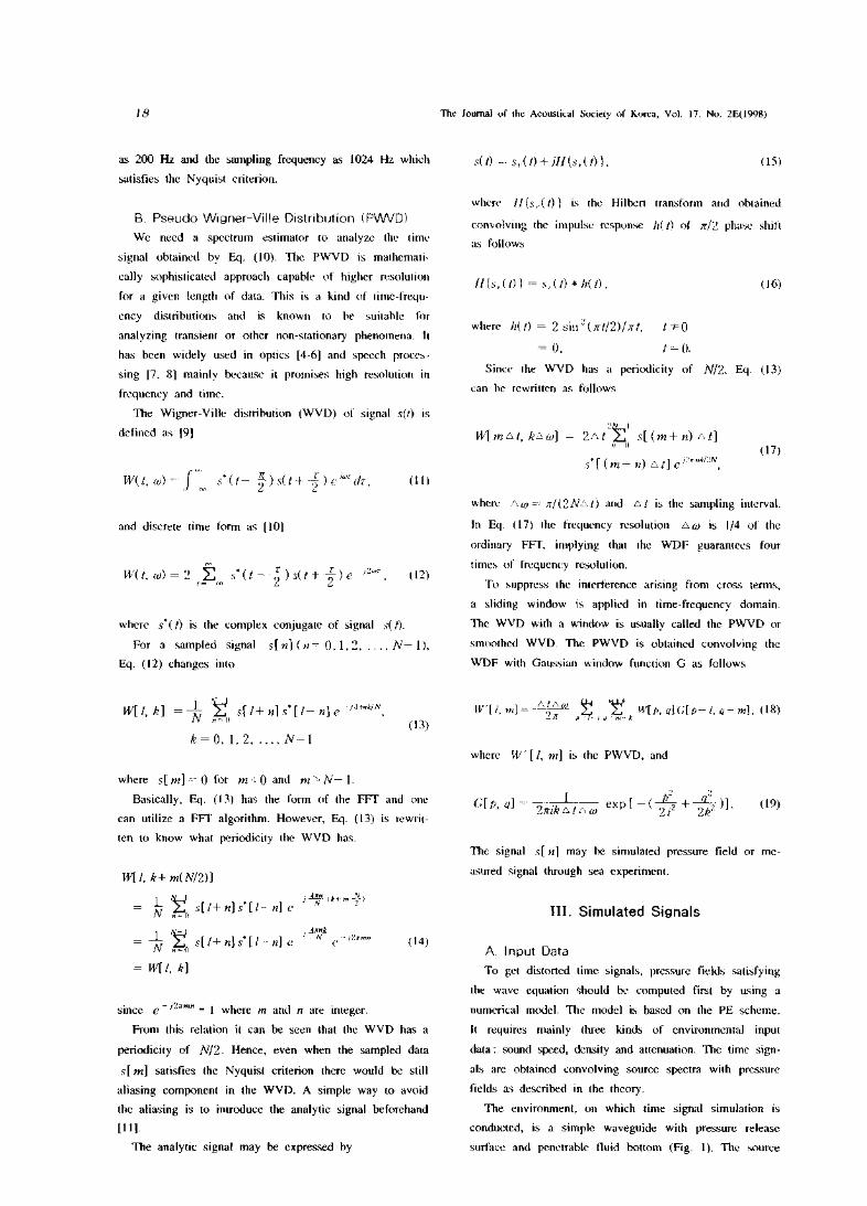
Figure 2 gives waveforms of upsweep and downsweep

signals over a period. Before the simulation of time sign

al a modified Hamming window is applied to the LFM

signals generated by Eq. (20). This leads to reduce the

energy leakage caused by the discontinuity of the finite

record of data. The modified Hamming window is taken

at the beginning and end of each 10% sweeping period

as hallowing:

(0.54-0.46 cos(lO^ZT)的)=1.0 O.ITGMO" (21)

l0.54 - 0.46cos[10^T-O/7l

This kind of window is preferable since it modifies relat

ively small number of the signal compared with the or

dinary window and so enables to keep LFM characterist

ics. Although the waveforms are different each other both

classes of the signals have identical power spectra.

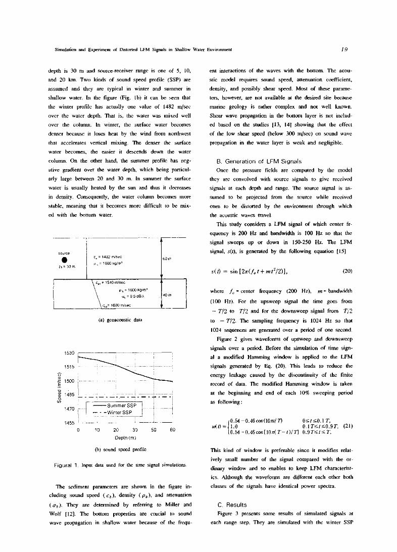
C. ResultsFigure 3 presents some resets of simulated signals at

each range step. They are simulated with the winter SSP


(a) upsweep

Time (sec)

응

2-一 을

V

욤

2흐

£

(b) downsweep

Figure 2. Waveform of the LFM signal swept up or down in150-250Hz.

where the source signal is swept up. The figures give

time-depth distributions of amplitude. The model inherently

calculates the amplitudes over the whole layers of the

water and sediment. In this study, however, the discussions

are limited to the water layer because the amplitudes in

the sediment layer are very small compared with those

in the water layer. In the figures simulated amplitudes are magnified as much as 105 (or 100 dB).

In the amplitude distribution at range 5 km, it can be

seen that there are noticeable constructive and destructive

interference caused by the interactions among the propa

gating rays of neighborin응 frequency. The amplitudes are

simulated with the upsweep signal. Some constructive

interference spans up to more than 100 milliseconds. The

interference may be accelerated by multi-paths of the

rays with same frequency.

The result at range of 10 km (Fig. 3b) shows that

there is still constructive interference and it is somewhat

symmetric over the water depth. The amplitudes are si-

m니ated with the upsweep signal. The duration time of

the interference tends to decrease compared with that at

range 5 km. In the result at range of 20 km (Fig. 3c),

the duration time of the interference decreases much more,

while the symmetricity increases over depth. The ampli

tudes are also simulated with the upsweep signal.

O

o

o

C

2

3

4

(E) 듬 9

。

200 400 600 800 1000"Time (msec)

60

& ■■■■曜프三二芸표^^■

-10 -5 0 5 10

(a) range 5 km, upsweep

o

o

o

o

o

C

1

2

3

4

5

6

(E)믐

(b) range 10 km, upsweep

o

o

o

O

1

2

3

4

(E) 즘

料

5Q

흔

罢초1

촐즈•项f

定

盘

宥度宿冶E,"

非•，急畧脅器a

기

蓄¥0

호.圣卷

薯

枝

“饵*

団

是츠틀-

":

.3盅亲圭뵤

总¥

.云처

手EEE

趙

比汪笙4-

i

I

鼾酝̂

課唸經K

(c) range 20 km, upsweep

Figure 3. Simulated amplitude distributions with time and depth for the various ranges. Amplitudes are simulated with the winter SSP and arc amplified by 105.


There exists noticeable destructive interference near the

surface and the bottom and this is explainable by the re

flection between the two interfaces. Large difference in

impedance between air and water causes nearly perfect re-

Hection with an angle-dependent phase shift. This mechan

ism makes the waves superpose themselves to result in

destructive interference. For the other interference between

water and bottom sediment the reflection coefficient can

be estimated based on the geoacoustic parameters in Fig.

1. At low grazing angles of below 5° it can be shown

that the reflection coefficient is almost 1.0 [16], implying

perfect reflection toward water layer and then destructive

interference between the incident and reflected waves.

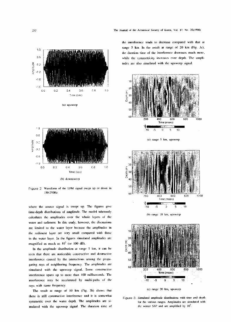
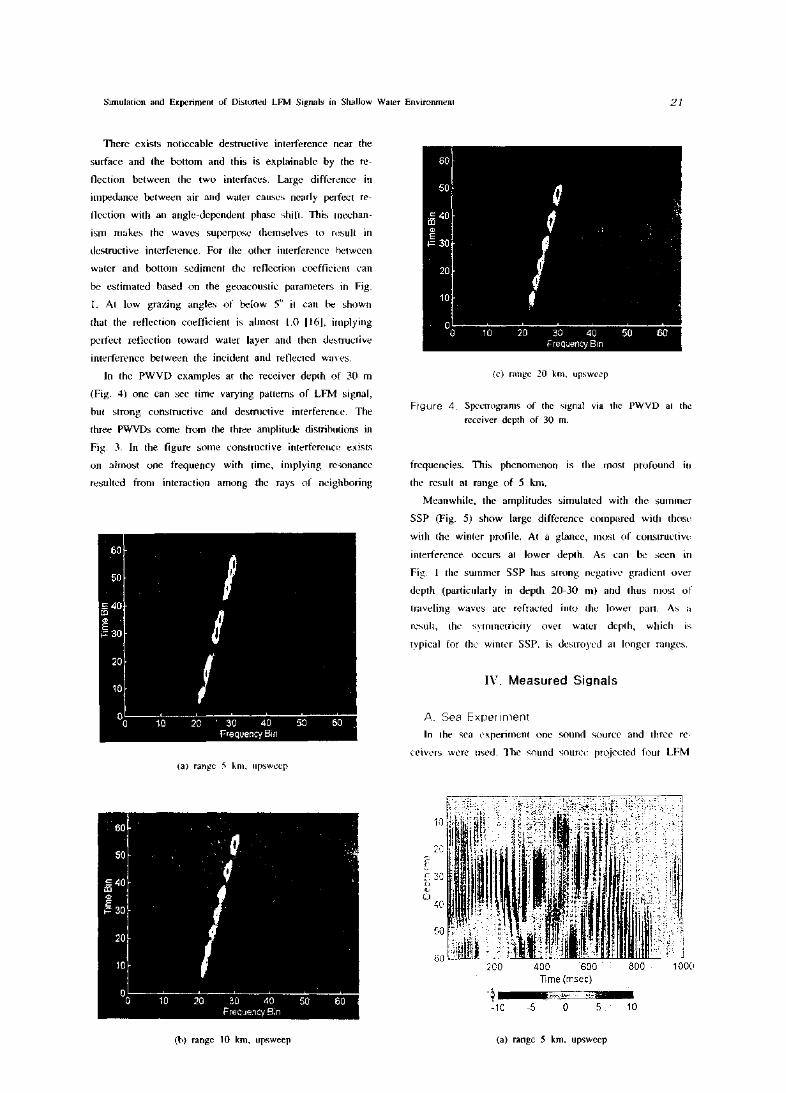
In the PWVD examples at the receiver depth of 30 m

(Fig. 4) one can see time varying patterns of LFM signal,

but strong constructive and destructive interference. The

three PWVDs come from the three amplitude distributions in

Fig. 3. In the figure some constructive interferencii exists

on almost one frequency with time, implying resonance

resulted from interaction among the rays of neighboring

20

10

앙 10 20—, 30 40 赤 60Frequency Bin

°0 10 20 30 40 50 60

Frequency Bin

(c) range 20 km, upsweep

Figure 4. Spectrograms of the signal via the PWVD at the receiver depth of 30 m.

frequencies. This phenomenon is the most profound in

the result at range of 5 km.

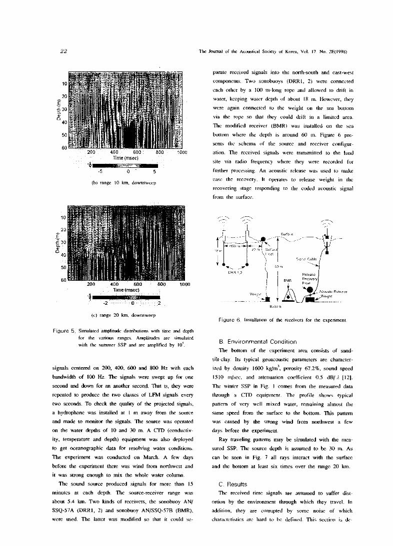
Meanwhile, the amplit나des simulated with the summer

SSP (Fig. 5) show large difference compared with those

with the winter profile. At a glance, most of consir나ctivc

interference occurs at lower depth. As can be seen in

Fig. 1 the summer SSP has strong negative gradient over

depth (particularly in depth 20-30 m) and thus most of

traveling waves are refracted into the lower part. As a

result, the symmetricity over water deph, which is

typical for the winter SSP, is destroyed at longer ranges.

IV. Measured Signals

A. Sea ExperimentIn the sea experiment one sound source and three re

ceivers were used. The sound source projected four LFM(a) range 5 km, upsweep

6 아

50

S40

e IF30

2 아

10

앙 10 20 30 40 50 60Frequency Bin

(b) range 10 km, upsweep (a) range 5 km, upsweep


o Vo

o

o

Q

o

1

2

3

4&

6

(E) £

聽

o 5

(b) range 10 km, downsweep

parate received signals into the north-south and east-west

components. Two sonobuoys (DRR1, 2) were connected

each other by a 100 m-long rope and allowed to drift in

water, keeping water depth of about 18 m. However, they

were again connected to the weight on the sea bottom

via the rope so that they could drift in a limited area.

The modified receiver (BMR) was installed on the sea

bottom where the depth is around 60 m. Figure 6 pre

sents the schema of the source and receiver configur

ation. The received signals were transmitted to the land

site via radio frequency where they were recorded for

further processing. An acoustic release was used to make

ease the recovery. It operates to release weight in the

recovering stage responding to the coded acoustic signal

from the surface.

(§£

믕

0

50

60200 400 :' 600 " 800 1000

Time (msec)

(c) range 20 km, downsweep

Figure 5. Simulated amplitude distributions with time and depth for the various ranges. Amplitudes arc simulated with the summer SSP and are amplified by 105.

signals centered on 200, 400, 600 and 800 Hz with each

bandwidth of 100 Hz, The signals were swept up for one

second and down for an another second. That is, they were

repeated to produce the two classes of LFM signals every

two seconds. To check the quality of the projected signals,

a hydrophone was installed at 1 m away from the source

and made to monitor the signals. The source was operated

on the water depths of 10 and 30 m. A CTO (conductiv

ity, temperature and depth) equipment was also deployed

to get oceanographic data for resolving water conditions,

The experiment was conducted on March. A few days

before the experiment there was wind from northwest and

it was strong enough to mix the whole water column.

The sound source produced signals for more than 15

minutes at each depth. The source-receiver range was

about 5.4 km. Two kinds of receivers, the sonobuoy AN/

SSQ-57A (DRR1, 2) and sonobuoy AN/SSQ-57B (BMR),

were used. The latter was modified so that it could se-

Figure 6. Installation of the receivers for the experiment.

B. Environmental Condition

The bottom of the experiment area consists of sand-

silt-clay. Its typical geoacoustic parameters are characterized by density 1600 kg/m3, porosity 67.2%, sound speed

1510 m/sec, and attenuation coefficient 0.5 dB/ A [12].

The winter SSP in Fig. 1 comes from the measured data

through a CTD equipment. The profile shows typical

pattern of very well mixed water, remainin응 almost the

same speed from the surface to the bottom. This pattern

was caused by the strong wind from northwest a few

days before the experiment.

Ray traveling patterns may be simulated with the mea

sured SSP. The source depth is assumed to be 30 m. As

can be seen in Fig. 7 all rays interact with the surface

and the bottom at least six times over the range 20 km.

C. Res니ts

The received time signals are assumed to suffer dist

ortion by the environment through which they travel. In

addition, they are corrupted by some noise of which

characteristics are hard to be defined. This section is de


voted to analyzing measured signals and comparing them

with the sim니ated ones.

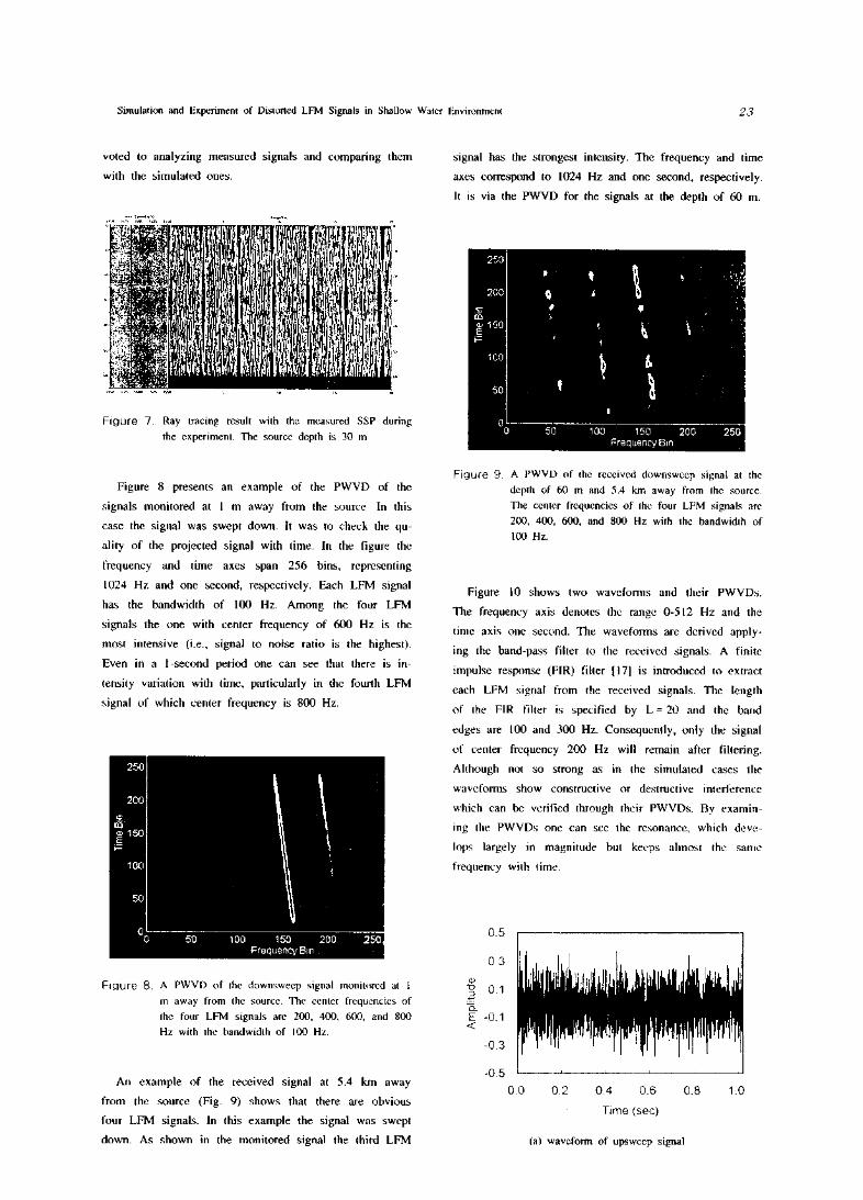
signal has the strongest intensity. The frequency and time

axes correspond to 1024 Hz and one second, respectively.

It is via the PWVD for the signals at the depth of 60 m.

O'-------------- ---------------------------- 「0 50 100 150 200 250!

Frequency Bin |

Fig니「e 7. Ray tracing result with the measured SSP during the experiment. The source depth is 30 m

Figure 8 presents an example of the PWVD of the

signals monitored at 1 m away from the source In this

case the signal was swept down. It was to check the qu

ality of the projected signal with time. In the figure the

frequency and time axes span 256 bins, representing

1024 Hz and one second, respectively. Each LFM signal

has the bandwidth of 100 Hz. Among the four LFM

signals the one with center frequency of 600 Hz is the

most intensive (i.e., signal to noise ratio is the highest).

Even in a 1 -second period one can see that there is in

tensity variation with time, particularly in the fourth LFM

signal of which center frequency is 800 Hz.

O'---------- ；-------------------------------0 50 100 150 200 250

Frequency Bin、

Figure 8. A PWVD of the downsweep signal monitored at 1 m away from the source. The center frequencies of the four LFM signals are 200, 400, 600, and 800 Hz with the bandwidth of 100 Hz.

An example of the received signal at 5.4 km away

from the source (Fig. 9) shows that there are obvious

four LFM signals. In this example the signal was swept

down. As shown in the monitored signal the third LFM

Figure 9. A PWVD of the received downsweep signal at the depth of 60 m and 5.4 km away from the source. The center frequencies of the four LFM signals arc 200, 400, 600, and 800 Hz with the bandwidth of 100 Hz.

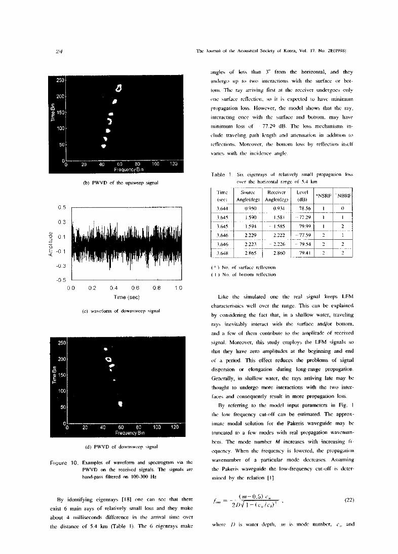
Figure 10 shows two waveforms and their PWVDs.

The frequency axis denotes the range 0-512 Hz and the

time axis one second. The waveforms are derived apply

ing the band-pass filter to the received signals. A finite

impose response (FIR) filter [17] is introduced to extract

each LFM signal from the received signals. The length

of the FIR filter is specified by L = 20 and the band

edges are 100 and 300 Hz. Consequently, only the signal

of center frequency 200 Hz will remain after filtering.

Although not so strong as in the simulated cases the

waveforms show constructive or destructive interference

which can be verified through their PWVDs. By examin

ing the PWVDs one can see the resonance, which deve

lops largely in magnitude but keeps almost the same

frequency with time.

5

3

1

1

3

°00

-0。

응

흐

u

-0.5 0.0 0.2 0.4 0.6 0.8 1.0

Time (sec)

(a) waveform of upsweep signal

24 The Journal of the Acoustical Society of Korea, Vol. 17, No. 2E(1998)

25°

o

o

w

0

5

0

2

1

1

£뜽트 50

50

angles of less than 3 from the horizontal, and they

undergo up to two interactions with the surface or bot

tom. The ray arriving first at the receiver undergoes only

one surface reflection, so it is expected io have minimum

propagation loss. However, the model shows that the ray,

interacting once with the surface and bottom, may have

minimum loss of 77.29 dB. The loss mechanisms in

clude traveling path length and attenuation in addition to

reflections. Moreover, the bottom loss by reflection itself

varies with the incidence angle.

0

L o

o20 40 60 80 100 120

Frequency Bin

(b) PWVD of the upsweep signal

① p

그-d&q

-0.50.0 0.2 0.4 0.6 0.8 1.0

Time (sec)

(c) waveform of downsweep signal

-

o

o

o

0

5

0

2

1 .■

1

드

와

u

af

50

이---------- ------ :------------------------0 20 .40 60 80 100 120一 Frequency Bin

(d) PWVD of downsweep signal

Figure 10. Examples of waveform and spectrogram via the PWVD on the received signals. The signals arc band-pass filtered on 100-300 Hz,

Table 1. Six eigenrays of relatively small propagation loss over the horizontal range of 5.4 km.

Time (see)

Source Anglc(dcg)

Receiver Angle(dcg)

Level (dB)

*NSRF NBRF

3.644 0.950 0.934 78.56 1 0

3.645 1.590 l.58l -77.29 1 1

3.645 1.594 -1.585 79.99 1 2

3.646 2.229 2.222 -77.59 2 1

3.646 -2.223 -2.226 -79.54 2 2

3.648 2.865 2.860 79,41 2 T

(* ) No. of surface reflection (I ) No. of bottom reflection

Like the simulated one the real signal keeps LFM

characteristics well over the range. This can be explained

by considering the fact that, in a shallow water, traveling

rays inevitably interact with the surface and/or bottom,

and a few of them contribute to the amplitude of received

signal. Moreover, this study employs the LFM signals so

that they have zero amplitudes at the beginning and end

of a period. This effect reduces the problems of signal

dispersion or elongation during long-range propagation.

Generally, in shallow water, the rays arriving late may be

thought to undergo more interactions with the two inter

faces and consequently result in more propagation loss.

By referring to the model inp니t parameters in Fig. 1

the low frequency cut-off can be estimated. The approx

imate modal solution for the Pakeris waveguide may be

truncated to a few modes with real propagation wavenum

bers. The mode number M increases with increasing fr

equency. When the frequency is lowered, the propagation

wavenumber of a particular mode decreases. Assuming

the Pakeris waveguide the low-frequency cut-off is deter

mined by the relation [1]

By identifying eigenrays [18] one can see that there

exist 6 main rays of relatively small loss and they make

about 4 milliseconds difference in the arrival time over

the distance of 5.4 km (Table 1). The 6 eigenrays make

爲=2加1-(&如)2 ' 心)

where D is water depth, m is mode number, and


cb are sound speeds in water and sediment, respectively.

Using the parameters in Fig. 1 it can be shown that the

first mode occurs at 16.4 Hz and the last at 245.7 Hz,

total of 8 modes being excited below 250 Hz. The de

structive or constructive interference may be also explain

ed by the interactions of these modes.

V. Conclusions

Time signals are simulated using an acoustic model

that employs the Fourier synthesis scheme. To obtain real

sea data, an acoustic experiment has been performed in a

shallow sea near Pohang, Korea.

The sim니ated time signals suffer great interference at

range of 5 km by the interactions of neighboring rays.

The simulated signals show great difference in amplitude

distributions by the variation of SSP. Although there is

constructive or destructive interference the received sign

als keep LFM characteristics. This property is thought to

be caused by a few rays of small loss which contribute

to the received signals in a shallow water environment.

Acknowledgements

The authors wo니d like to appreciate Prof. J. Y. Na

in Hanyang University for his useful comments. They

wish to give thanks to Dr. J. J. Jeon in Agency for

Defense Development for releasing programs on spectral

estimation. Special thanks are directed to Dr. M. Collins

in Naval Research Laboratory, USA for releasing a

model that made it possible to simulate time signals.

Their appreciation is extended to anonymous reviewers

for their kind suggestions and comments.

References

1. F. B. Jensen, W. A. Kuperman, M, B. Porter, and H. Schmidt, "Broadband Modeling,'' in Computational Ocean Acoustics, A1P Press, Woodbury, NY, 1994.

2. R. L. Fi미d, E. J. Yoerger, and P. K. Simpson, uPerfor- mance of Neural Networks in Classifying Environmentally Distorted Transient Signals,'' Oceans'90 Proc., pp. 13-17, 1991.

3. A. V. Oppenheim and R. W. Schafer, Discrete-Time Signal Processing, Prentice Hall, New Jersey, 1989.

4. M. J. Bastians, "The Wigner Distribution Function Applied to Optic Signals and Systems,Optics Comm., v이.25(1), pp.26-30, 1978.

5. M. J. Bastians, "Wigner Distribution Function and Its Application to First-Order Optics,” J. Optic. Soc. Am., vol.69 (12), pp.1710-1716, 1979.

6. H. O. Bartlct, K. H. Brenner, and A. W. L사un저nn, "The Wigner Distribution Function and Its Optical Production,"

Optics Comm., vol.32(11), pp.32-38, 1980.7. M. Riley, Speech Time-Frequency Representations, Kluwer

Academic Publishers, 1989.8. E. Velez and R. Absher, ''Transient Analysis of Speech

Signals Using the Wigner Time-Frequency Representation,'' IEEE Inti. Conf. Acoustics, Speech and Signal Processing, vol.4, pp.2242-2245, 1989.

9. E. Wigner, “On the Quantum Correction for Thermodynamic Equilibrium,'' Physic Review, vol.40, pp.740-759, 1932.

10. rf. Classen and W. Mecklcnbrauker, "The Wigner Distribut- ion-A Tool for Time-Frequency Signal Analysis/' Philips J. Res., vol.35, part I : 217-250, part II : 276-300, part III : 372-389, 1980.

11. J. Ville, uTheoric et Applications de la Notion de Signal An- alytique/' Cables et Transmission, vol.29(1), pp.61-74, 1948.

12. J. F. Miller and S. N. Wolf, "Modal Acoustic Transmission Loss (MOATL) : A Transmission-Loss Computer Program Using a Normal-Mode Mod이 of the Acoustic Field in the Ocean,', Naval Research Lab., Rep. No. 8429, pp. 1-126, 1980.

13. F, D. Tappcrt and T. Y. Yamamoto, "An issue (sedim이u volume fluctuations) and a non-issue (shear wave propa음at- ion) in shallow water acoustics," J. Acoust. Soc. Am., vol. 93, p.2268A, 1993.

14. C. T. Tindle and 乙 Y. 가］ang, "An equivalent fluid approximation for a low shear speed ocean bottom,'* J. Acoust. Soc. Am., voL91, pp.3248-3256, 1992.

15. R. O. Nielson, Sonar Signal Processing, Artech House Inc., Boston, 1991.

16. Y. N. Na, Classification of Environmentally Distorted Acoustic Signals tn Shallow Water Usin을 Neural Networks, Ph.D. Thesis in Pukyong National University, Pusan, pp. 1-202, 1998.

17. S. D. Steams and R. A. David, Signal Processing Algorithms in Fortran and C, Prentice Hall International Inc., pp.1-331, 1993.

18. S.W. Shin, Study on Ray-Method Mod이 based on Constant-Gradient Sound Speed, Master Thesis in Hanyang University, pp. 1-54, 1994.

▲丫。냐ng~Nam Na

Senior Research Scientist, Agency for Defense Develop

ment (Vol. 15, No. 3E, 1996)

AMun-Sub Jurng

Senior Research Scientist, Agency for Defense Develop

ment (Vol. 13, No. 2E, 1994)

▲Taebo Shim

Chief Research Scientist, Agency for Defense Develop

ment (Vol. 14, No. 2E, 1995)

▲ Chun-D니ck Kim

Professor, Department of Electrical Engineering Pukyong

National University (Vol. 15, No. 3E, 1996)

jako199811920205116.pdf - korea science

Documents