ionic wave propagation along actin filaments

Ionic Wave Propagation along Actin Filaments

J. A. Tuszynski,* S. Portet,* J. M. Dixon,* C. Luxford,* and H. F. Cantielloy

*Department of Physics, University of Alberta, Edmonton, Alberta T6G 2J1, Canada; and yMassachusetts General Hospitaland Harvard Medical School, Charlestown, Massachusetts 02129 USA

ABSTRACT We investigate the conditions enabling actin filaments to act as electrical transmission lines for ion flows alongtheir lengths. We propose a model in which each actin monomer is an electric element with a capacitive, inductive, and resistiveproperty due to the molecular structure of the actin filament and viscosity of the solution. Based on Kirchhoff’s laws taken in thecontinuum limit, a nonlinear partial differential equation is derived for the propagation of ionic waves. We solve this equation intwo different regimes. In the first, the maximum propagation velocity wave is found in terms of Jacobi elliptic functions. In thegeneral case, we analyze the equation in terms of Fisher-Kolmogoroff modes with both localized and extended wavecharacteristics. We propose a new signaling mechanism in the cell, especially in neurons.

INTRODUCTION

The cytoskeleton is a major component of all living cells. It

is made up of three different types of filamental structures,

including actin-based microfilaments (MFs), intermediate

filaments (e.g., neurofilaments, keratin), and tubulin-based

microtubules (MTs). All of them are organized into net-

works, which are interconnected through numerous partic-

ular proteins, and which have specific roles to play in the

functioning of the cell. The cytoskeletal networks are mainly

involved in the organization of different directed movements

in cell migration, cell division, or in the internal transport of

materials. Polymerization of MFs is responsible for cell

migration and for the remodeling of the leading edge of cells.

MTs attach to the chromosomes and mediate cell division.

Molecular motors are protein complexes that are associated

with the cytoskeleton and drive organelles along MTs and

MFs in a ‘‘vectorial’’ transport.

Actin is the most abundant protein in the cytoplasm of

mammalian cells, accounting for 10–20% of the total

cytoplasmic protein content. Actin exists either as a globular

monomer (Fig. 1), i.e., as the so-called G-actin, or as

a filament, i.e., an MF: the globular monomers polymerize

into polar two-stranded helical polymers, MFs, also called

F-actin. Under physiological conditions, actin filaments are

one-dimensional polymers that behave as highly charged

polyelectrolytes (Cantiello et al., 1991; Kobayasi, 1964;

Kobayasi et al., 1964). The linear charge density of F-actin is

estimated theoretically to be 4 3 103 e/mm in vacuum, and

although lower than that of DNA at physiological pH, it may

support ionic condensation in buffer solutions as originally

predicted by Manning’s condensation theory (Manning,

1978). This has recently been confirmed experimentally by

light scattering (Tang and Janmey, 1996) although other

experimental work arrives at linear charge densities that

are much higher (Cantiello et al., 1991) of order 1.65 3 105

e/mm. The latter value of charge density is consistent with

other experiments and is associated with a highly uncom-

pensated charge density of actin in solution. These experi-

ments include the coexistence of different electric (Kobayasi,

1964; Kobayasi et al., 1964) and magnetic (Torbet and

Dickens, 1984) dipole moments in F-actin, the anomalous

Donnan potential, nonlinear electro-osmotic behavior of

actin filaments in solution (Cantiello et al., 1991), and the

ability of F-actin to support ionic condensation-based waves

(Lin and Cantiello, 1993).

Many years ago, Manning (1978) postulated an elegant

theory, which stated that polyelectrolytes may have

condensed ions in their surroundings. According to Mann-

ing’s hypothesis, counterions ‘‘condense’’ along the stretch

of polymer, if a sufficiently high linear charge density is

present on the polymer’s surface. Thus, a linear polymer may

be surrounded by counterions from the saline solution such

that counterions are more closely surrounding the polymer’s

surface, and co-ions of the salt solution are repelled such that

a depletion area is also created. Some important details of the

ion distribution in polyelectrolytes regarding Manning’s

condensation theory can be found in Le Bret and Zimm

(1984). The sum of surface charges and associated counter-

ions drops to values given by a formula that depends on the

valence of the counterions and the Bjerrum length. This

parameter, in turn, is a phenomenological property of the

ion’s ability to compensate for the surface charges, depend-

ing on the solvent and temperature of the solution. Bjerrum

developed a modification of the Debye-Huckel theory in

1926 for ion-pair formation provided that the ions are small,

they are of high valence, and the dielectric constant of the

solvent is small (see MacInnes, 1961, for a comprehensive

explanation of derivations of relevant equations). The

Bjerrum length is the distance at which the Coulomb energy

of the screened charges equals kBT, the thermal energy,

creating an equilibrium under which the charges would not

preferentially move from that equilibrium. See Eq. 1 below.

Submitted July 16, 2003, and accepted for publication November 14, 2003.

Address reprint requests to J. A. Tuszynski, E-mail: [email protected].

J. M. Dixon’s permanent address is Dept. of Physics, University of

Warwick, Coventry CV4 7AL, UK.

� 2004 by the Biophysical Society

0006-3495/04/04/1890/14 $2.00

1890 Biophysical Journal Volume 86 April 2004 1890–1903

The cylindrical volume of depleted ions outside the cloud

of ions surrounding the polymer serves as an electrical shield.

Thus, the ‘‘cable-like’’ behavior of such a structure is

supported by the polymer itself and the ‘‘adsorbed’’ counter-

ions, which for all practical purposes are ‘‘bound’’ to the

polymer. The strength of this interaction is such that even

under infinite dilution conditions (i.e., ionic strength*0), the

counterions are still attracted to the polymer and do not diffuse

out from the polymer’s vicinity. Although this theory was

originally postulated for such polyelectrolytes as DNA, the

same applies to highly charged one-dimensional polymers.

Available atomic models of actin are largely derived from

the crystal structure of the monomer and primary sequencing

(Holmes et al., 1990; Kabsch et al., 1990) and not from

actin’s behavior in solution. Thus there is the possibility of

other explanations to reconcile the discrepancy between

theoretical and experimentally determined charge densities

of actin. This could include highly nonlinear interactions

between the hydrated molecule and its surrounding counter-

ions, which are not taken into account in the atomic models

above and which may play an important role in the

electrodynamic properties of proteins in solution (Rullman

and van Duijnem, 1990). It is to be expected, for example,

that, because of the helical nature of the F-actin (Holmes

et al., 1990), the distribution of counterions will be

nonuniform along the polymer’s length. As a consequence,

spatially dependent electric fields could be present and

arranged in peaks and troughs as originally postulated by

Oosawa (1971). This might imply large changes in the

density of small ions around the polymer with a large

dielectric discontinuity in the ionic distribution (Kabsch

et al., 1990; Anderson and Record, 1990).

The double helical structure of the filament provides

regions of uneven charge distribution such that pockets of

higher and lower charge density may be expected. The charge

distribution can be envisioned as a string of cola bottles inside

an elastic tube. As the bottles are pushed into the cylinder, the

outer shape of the wider parts of each bottle may provide the

shortest distance to the cylinder’s wall, and thus the thinnest

charge density. The thinner sections of each bottle provide

‘‘deeper’’ pockets where more ions can be trapped. The

distance between ion clusters in the pockets, which in reality

are immersed in water with very specific properties not

shared by the bulk solution, will make ions move up and

down the slopes of the surface of the bottle. This uneven ionic

distribution along a short stretch of the polymer (likely the

average pitch 35–40 nm) may be considered a linear unit of

the circuit to be modeled. This ionic distribution makes two

essential contributions to the nonlinear electrical components

of the model. First, the nonlinear capacitor, which is

associated with the spatial difference in charges between

the ions located in the outer and inner regions of the polymer.

Second, any charge movement tending to dissipate this local

gradient (reversibly) generates a secondary electromotive

force due to the charge movement, namely a local current.

This is the main contribution to the inductance of the single

stretch of polymer.

F-actin, being a highly charged polyelectrolyte, contains

a fraction of its surrounding counterions in the form of

a condensed cloud about its surface. Such a cloud may be

highly insensitive to large changes in the ionic strength of the

surrounding saline solution (Oosawa, 1970; Manning, 1969;

Zimm, 1986).

The Bjerrum length, lB, describes the distance beyond

which thermal fluctuations are stronger than the electrostatic

attractions or repulsions between charges in solution whose

dielectric constant is e. It is defined by

e2

4pee0lB

¼ kBT (1)

for a given temperature T in Kelvin. Here e is the electroniccharge, e0 the permittivity of the vacuum, and kB is

Boltzmann’s constant. For a temperature of 293 K, it is

readily found that lB ¼ 7.13 3 10�10 m. Counterion

condensation occurs when the mean distance between

charges, b, is such that lB/b ¼ S[ 1. Each actin monomer

carries an excess of 14 negative charges in vacuum, and

accounting for events such as protonation of histidines, and

assuming there to be 3 histidines per actin monomer, there

exist 11 fundamental charges per actin subunit (Tang and

Janmey, 1996). Assuming an average of 370 monomers per

mm, we find that there is ;4 e/nm in agreement with an

earlier statement. Thus we expect a linear charge spacing of

b¼ 2.53 10�10 m, so S¼ 2.85. As the effective charge, qeff,or renormalized rod charge is the bare value divided by S, wefind qeff ¼ 3.93 e/monomer.

Assuming for simplicity a linear charge distribution about

the actin filament, the linear charge density, j, is much

FIGURE 1 Ribbon diagram of an actin monomer (Kabsch et al., 1990)

(Protein Data Bank identification: 1ATN). Figure produced with RasMol.

Ionic Wave Propagation along Actin 1891

Biophysical Journal 86(4) 1890–1903

greater than 1/z, where z is the valence of the counterions insolution. The parameter, j, is given by

j ¼ e2

4pe0erkBTb; (2)

where e is the electronic charge, er the dielectric constant

of water, and b the average axial spacing of charges on

the polyelectrolyte (Zimm, 1986). The parameter, j, was

calculated to be 110 for actin filaments (with z¼ 1 for H1and

K1 ions) and so j � 1=z (Lin and Cantiello, 1993). Thus

;99% of the counterion population is predominantly

constrained within a radius of 8 nm (Pollard and Cooper,

1986) round the polymer’s radial axis (Zimm, 1986).

Significant ionic movements within this ‘‘tightly bound’’

ionic cloud are therefore allowed along the length of the actin

(Fig. 2), provided that it is shielded from the bulk solution

(Oosawa, 1970; Parodi et al., 1985).

The electro-conductive medium is a condensed cloud of

ions surrounding the polymer. To be electrically insulated

from the bulk of the solution (although not mandatory), there

should be some sort of shielding from the bulk solution,

which acts as a common ground to the ‘‘transmission line’’.

The presence of one or more layers of waters of hydration

around the protein filament may provide additional screen-

ing. In earlier publications (Hameroff et al., 2002; Hagan

et al., 2002), some of the present authors have suggested that

such a condensation/ionic cloud/plasma phase around

microtubules may help shield not only signaling but

quantum states from external decoherence. In this connec-

tion, the transfer of information by quantum coherence-

based phenomena requires that the system be isolated from

the environment such that the ‘‘energy’’ does not dissipate.

This would imply that efficient transfer of energy from

‘‘energized groups’’ that can only be in resonating

frequencies when they are close to each other (Davydov,

1982; Frohlich, 1975, 1984). In the context of microtubular

‘‘kink’’ soliton behavior, the calcium ions adsorbed to one

region of each tubulin monomer may form a functional

dipole, which is shifted in space by energizing the monomer

by GTP binding (Sataric et al., 1993). The dipolar moments

of each heterodimer (a-, b-tubulins) would be switched in

the microtubule, such that a change in structural local

stability is transferred spatially along the microtubular

structure. This is the basis of the proposed information

transfer mechanism, which although highly probable, is

different from the ionic waves supported by actin filaments.

It is important to note, however, that ionic waves might also

be supported by microtubules, a phenomenon that will re-

quire experimental proof. Furthermore, quantum models

supported by microtubular structures might also exist that

imply a particular state of water in the microtubular structure

that indeed has properties largely different from those ex-

pected by free solution (see Mavromatos, 1999).

Bearing in mind the sheath of counterions around the ac-

tin filament, we see that effectively actin polymers may act

as biological ‘‘electrical wires’’, which can be modeled as

nonlinear inhomogeneous transmission lines that are able

to propagate nonlinear dispersive solitary waves (Kolosick

et al., 1974; Ostrovskii, 1977) in the form of solitons

(Lonngren, 1978; Noguchi, 1974). It has been proposed that

such solitons, localized traveling waves, exist in many

biological systems and, in fact, have earlier been postulated

in linear biopolymers such as MTs (Sataric et al., 1993) and

DNA (Baverstock and Cundall, 1988). Interestingly, both

solitary waves (Lin and Cantiello, 1993) and liquid crystal

formation (Coppin and Leavis, 1992; Furukawa et al., 1993)

have been observed in actin filaments possibly providing

a potentially fruitful environment for innovative biotechno-

logical applications.

In this article we develop a model based on the

transmission line analogy with inductive, resistive, and

capacitive components. The physical significance of each of

the components, for each section of the electrical network,

will be described below. This way we will investigate the

nature of nonlinear ionic waves propagating along an actin

filament in solutions containing counterions as would be

found under realistic physiological conditions.

FIGURE 2 Nonlinear dispersive solitary waves traveling

along an actin filament.

1892 Tuszynski et al.


CHARACTERIZATION OF THE TRANSMISSIONLINE COMPONENTS

In this section, we describe the electrical components that

make up our nonlinear circuit, which mimics the behavior of

an actin filament in solution. As the filament core is separated

from the rest of the ions in the bulk solution by the

counterion condensation cloud, we expect this cloud to act as

a dielectric medium between the two. This cloud provides

both resistive and capacitive components for the behavior of

the monomers that make up the actin filament. Ion flow is

expected at a radial distance from the center of the filament,

which is approximately equal to the Bjerrum length. The

inductive component to the electrical properties of ionic

waves is due to actin’s double-stranded helical structure that

induces the ionic flow in a solenoidal manner. Below we

discuss the origin of each electrical component in turn.

The effective Bjerrum length of an actin filament in

solution was derived in Lin and Cantiello (1993) with data

originally obtained in Cantiello et al. (1991). In that study,

a Donnan potential of ;�3.93 mV was found for actin in

solution.

The origin of capacitance

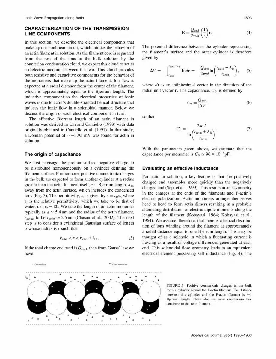
We first envisage the protein surface negative charge to

be distributed homogeneously on a cylinder defining the

filament surface. Furthermore, positive counterionic charges

in the bulk are expected to form another cylinder at a radius

greater than the actin filament itself, ;1 Bjerrum length, lB,

away from the actin surface, which includes the condensed

ions (Fig. 3). The permittivity, e, is given by e ¼ e0er, whereer is the relative permittivity, which we take to be that of

water, i.e., er ¼ 80. We take the length of an actin monomer

typically as a ’ 5:4 nm and the radius of the actin filament,

ractin, to be ractin ’ 2:5 nm (Chasan et al., 2002). The next

step is to consider a cylindrical Gaussian surface of length

a whose radius is r such that

ractin\r\ractin 1 lB: (3)

If the total charge enclosed is Qencl, then from Gauss’ law we

have

E ¼ Qencl

2pel1

r

� �r: (4)

The potential difference between the cylinder representing

the filament’s surface and the outer cylinder is therefore

given by

DV ¼ �ðractin1lB

ractin

E:dr ¼ �Qencl

2pelln

ractin 1 lB

ractin

� �; (5)

where dr is an infinitesimal vector in the direction of the

radial unit vector r. The capacitance, C0, is defined by

C0 ¼Qencl

jDVj (6)

so that

C0 ¼2pel

lnractin 1 lB

ractin

� � : (7)

With the parameters given above, we estimate that the

capacitance per monomer is C0 ’ 963 10�6pF.

Evaluating an effective inductance

For actin in solution, a key feature is that the positively

charged end assembles more quickly than the negatively

charged end (Sept et al., 1999). This results in an asymmetry

in the charges at the ends of the filaments and F-actin’s

electric polarization. Actin monomers arrange themselves

head to head to form actin dimers resulting in a probable

alternating distribution of electric dipole moments along the

length of the filament (Kobayasi, 1964; Kobayasi et al.,

1964). We assume, therefore, that there is a helical distribu-

tion of ions winding around the filament at approximately

a radial distance equal to one Bjerrum length. This may be

thought of as a solenoid in which a fluctuating current is

flowing as a result of voltage differences generated at each

end. This solenoidal flow geometry leads to an equivalent

electrical element possessing self inductance (Fig. 4). The

FIGURE 3 Positive counterionic charges in the bulk

form a cylinder around the F-actin filament. The distance

between this cylinder and the F-actin filament is ;1

Bjerrum length. There also are some counterions that

condense to the actin filament.



magnetic induction field,B, inside such a solenoid, parallel toits axis is given by

B ¼ mN

lIz; (8)

where z is a unit vector along the axis of the solenoid, N is

the total number of effective turns of the coil (the number of

windings of the helical distribution of ions around the

filament), m is the magnetic permeability, and I the current

through the coil. From Faraday’s law the emf generated is

emf ¼ � mN2A

l

� �dI

dt; (9)

where A is the cross-sectional area of the effective coil given

by

A ¼ p ractin 1 lBð Þ2: (10)

The potential drop across an inductance, L, is given by

emf ¼ � LdI

dt

� �; (11)

so we may define an effective inductance for the actin

filament in solution by

L ¼ mN2A

l; (12)

where l is the length of the F-actin. The number of turns,

N ¼ a/rh, is approximated by simply working out how many

ions could be lined up along the length of a monomer. We

would then be approximating the helical turns as circular

rings lined up along the axis of the F-actin. This is surely an

overestimate to the number of helical turns per monomer, but

it is certainly within reason for our purposes as an initial

approximation. We also take the hydration shell of the ions

into account in our calculation. This shell results when an ion

is inserted into a water configuration, changing the structure

of the hydrogen bond network. A water molecule will re-

orient such that its polarized charge concentration faces the

opposite charge of the ion. As the water molecules orient

themselves toward the ion, they break the hydrogen bonds to

their nearest neighbors. The hydration shell is then the group

of water molecules oriented around an ion. A rough estimate

for the size of a typical ion in our physiological solution, with

a hydration shell, is rh ’ 3:63 10�10m. This is the ap-

proximate radius of the first hydration shell of sodium ions.

Substituting these values into Eq. 12, we readily find that

L ’ 1:7 pH for the length of the monomer.

Modeling the resistance component

The current, I, between the two concentric cylinders is

I ¼ðJ:da ¼ s

ðE:da ¼ s

ell; (13)

where we have related linearly the current density, J, to the

electric field by J ¼ sE, s being the conductivity and the

integral is over an infinitesimal area, da, on the surface of

the outer cylinder pointing radially outward. Using Ohm’s

law, including the potential difference in Eq. 5 and the

current I in Eq. 13, the magnitude of the resistance, R ¼ V/I,is given by

R ¼ r lnððractin 1 lBÞ=ractinÞ2pl

; (14)

where r is the resistivity. To a first-order approximation, the

conductivity of a solution as a function of salt concentration,

c, obeys the relationship

sðcÞ ’ ^0c; (15)

where ^0 is a positive constant that does not depend on

concentration but only on the type of salt. Typically, for K1

and Na1, intracellular ionic concentrations are 0.15 M and

0.02 M, respectively (Tuszynski and Dixon, 2001). The

^0 parameters for the two ions are

^K1

0 ’ 7:4ðVmÞ�1M

�1

^Na1

0 ’ 5:0ðVmÞ�1M

�1: (16)

Kohlrausch’s law states that the molar conductance of a salt

solution is the sum of the conductivities of the ions com-

prising the salt solution. Thus

s ’ ^K1

0 cK1 1 ^Na1

0 cNa1 ¼ 1:21ðVmÞ�1: (17)

Using Eq. 17 with r ¼ s�1, the resistance estimate in Eq. 14

becomes R ¼ 6.11 MV, which is very much less, as we

would expect, than pure water since Rwater ¼ 1.83 106 MV,

the physiological solution being much more conductive than

pure water.

FIGURE 4 Dipole moment of a dimer is represented by the arrow.



Effective values for F-actin

In the analysis of F-actin surrounded by saline solution (see

Fig. 5), it is useful to have values for resistance, inductance,

and capacitance for the entire filament. This amounts to

finding effective values using the appropriate addition rules.

Referring to Fig. 6, we see that we must include both the

parallel and series contributions to the resistance, that the

total capacitance is a parallel-addition formula, and the total

inductance is obviously a strictly series contribution. For

a filament containing nmonomers, we would get an effective

resistance, inductance, and capacitance, respectively, such

that:

Reff ¼ +n

i¼1

1

R2;i

� ��1

1 +n

i¼1

R1;i (18)

Leff ¼ +n

i¼1

Li (19)

and

Ceff ¼ +n

i¼1

C0;i; (20)

where R1,i ¼ 6.113 106 V and R2,i ¼ 0.93 106 V such that

R1,i ¼ 7R2,i. The reader should note that we have used R1,i ¼R1, R2,i ¼ R2, Li ¼ L, and C0,i ¼ C0.

For a 1 mm of the actin filament, we find therefore

Reff ¼ 1:23 109V

Leff ¼ 3403 10�12

H

Ceff ¼ 0:023 10�12

F:

FIGURE 5 F-actin surrounded by water molecules and

counterions.

FIGURE 6 An effective circuit diagram for the nth

monomer between the dotted lines. In is the current through

the inductance L and resistance R1.



MODELING ACTIN FILAMENTS AS NONLINEARLRC TRANSMISSION LINES

In this section, we set up an electrical model of the actin

filament, using inductive, capacitive, and resistive compo-

nents, based on the ideas developed in the last section.

Basically, we apply Kirchhoff’s laws to that section of the

effective electrical circuit for one monomer, M, which

involves coupling to neighboring monomers (see Fig. 6). We

then take the continuum limit, assuming a large number of

monomers along an actin filament.

We expect a potential difference between one end of the

monomer generated between the filament core and the ions

lying along the filament at one Bjerrum length away. We

have already seen that these ‘‘Bjerrum ions’’ generate a time-

dependent current by movement along helical paths and

hence are responsible for the inductance, L. Due to viscosity,we also anticipate a resistive component to these currents,

which we insert in series with L and denote it by R1 (see Fig.

6). In parallel to these components, there exists a resistance,

which we call R2, acting between the Bjerrum ions and the

surface of the filament. In series with this resistance, we have

a capacitance, C0. We assume that the charge on this

capacitor varies in a nonlinear way with voltage much like

the charge-voltage relation for a reversed-biased pn diode

junction (Ma et al., 1999; Wang et al., 1999). Thus we

suppose, for the nth monomer,

Qn ¼ C0ðVn � bV2

nÞ; (21)

where b is expected to be small.

From Kirchhoff’s laws, using Fig. 6, if In is the current

through the inductance, L, and the resistor R1 and In�1, is that

flowing along AB, the current in DB must be In � In�1. For

the section BC of the nth monomer,

vn � vn1 1 ¼ LdIndt

1 InR1; (22)

where vn and vn11 are the voltages across AE and CF,respectively (see Fig. 6). Similarly, if the voltage across the

capacitor is Vn 1 V0, where V0 is the bias voltage of the

capacitor, we have

vn ¼ R2ðIn�1 � InÞ1V0 1Vn: (23)

Furthermore, the current through the section BD must be the

rate of change of charge, Qn, so that

In�1 � In ¼dQn

dt: (24)

From Eq. 22 we have

LdIn�1

dt¼ vn�1 � vn � In�1R1 (25)

and

LdIndt

¼ vn � vn1 1 � InR1: (26)

From Eq. 24,

Ld2Qn

dt2 ¼ L

dIn�1

dt� L

dIndt

; (27)

so from Eqs. 25, 26, and 27 we have

Ld2Qn

dt2 ¼ vn�1 � vn � In�1R1 � ðvn � vn1 1 � InR1Þ

¼ vn1 1 1 vn�1 � 2vn 1R1ðIn � In�1Þ: (28)

Using Eq. 23 in Eq. 28, we find

Ld2Qn

dt2 ¼ LC0ðVn � bV

2

nÞ

¼ Vn1 1 1Vn�1 � 2Vn � R1C0

d

dtðVn � bV2

nÞ

� R2C0 2d

dtðVn � bV

2

nÞ �d

dtðVn1 1 � bV

2

n1 1Þ�

� d

dtðVn�1 � bV

2

n�1Þ�:

(29)

A continuum approximation is now made by writing Vn ¼V and using a Taylor expansion in a small spatial parameter

a to give

Vn1 1 ¼ V1 a @xVð Þ1 a2

2!ð@xxVÞ1

a3

3!ð@xxxVÞ

1a4

4!ð@xxxxVÞ1 � � � (30)

and

Vn�1 ¼ V � að@xVÞ1a2

2!ð@xxVÞ �

a3

3!ð@xxxVÞ

1a4

4!ð@xxxxVÞ � � � � ; (31)

where, at this stage, we retain all derivatives up to the fourth

order. From Eqs. 30 and 31 we find that

Vn1 1 � 2Vn 1Vn�1 ¼ a2ð@xxVÞ1

2a4

4!ð@xxxxVÞ: (32)

Using Eqs. 32, 30, and 31, Eq. 30 becomes



We consider variations in time to be small compared to the

constant background voltage and the nonlinear term in the

capacitance to be of second order. Postulating that typical

time derivatives are of order e (where e is some small

parameter), the nonlinear voltage terms in the capacitance of

order e2 and a of order e, we retain only terms up to e3 in Eq.33 to finally obtain:

LC0

@2V

@t2 ¼ a

2ð@xxVÞ1R2C0

@

@tða2ð@xxVÞÞ

� R1C0

@V

@t1R1C02bV

@V

@t; (34)

which will form the basis of our physical analysis of the ion

conduction problem.

ANALYSIS OF THE VOLTAGE EQUATION

As a result of applying an input voltage pulse with an

amplitude of ;200 mV and a duration of 800 ms to an actin

filament, electrical signals were measured at the opposite end

of the actin filament (Lader et al., 2000). This experiment

indicates that actin filaments can support ionic waves in the

form of axial nonlinear currents. The current measured in the

process reached a peak value of ;13 nA and it lasted for

;500 ms. In a related earlier experiment (Lin and Cantiello,

1993), the wave patterns observed in electrically stimulated

single actin filaments were remarkably similar to recorded

solitary wave forms from various experimental studies on

electrically stimulated nonlinear transmission lines (Kolo-

sick et al., 1974; Lonngren, 1978; Noguchi, 1974). Con-

sidering the actin filament’s highly nonlinear complex

physical structure (Pollard and Cooper, 1986) and thermal

fluctuations of the counterionic cloud from the average dis-

tribution (Oosawa, 1970, 1971), the observation of soliton-

like ionic waves is consistent with the idea of actin filaments

functioning as biological transmission lines.

Indeed, the soliton conformation theory for proteins

involves charge displacement for ‘‘resonant’’ states within

a particular structure as predicted by Davydov (see Davydov,

1982). However, in the case of actin in solution, the soliton

behavior envisaged in our model is constrained to the ion

clouds and represents the ‘‘convective movement of ions’’

along a one-dimensional polymer.

Based on the argument put forward above, in this section

we analyze the solutions of Eq. 34 by looking for traveling

waves. Thus the voltage becomes a function of an

independent variable, the moving coordinate, z ¼ x � v0t,so that V ¼ V(z) and the equation becomes an ordinary

differential equation, albeit nonlinear, where v0 is the

propagation velocity. Equation 34 then becomes

R2a2v0

L

d3V

dz3 1 ðv20 � c20a

2Þ d2V

dz2

12bR1v0

LV � R1v0

L

� �dV

dz¼ 0: (35)

Here the parameter c20 is defined by

c2

0 ¼1

LC0

: (36)

Equation 35 may be integrated once to yield

R2a2v0

L

d2V

dz2 1 ðv20 � c

2

0a2Þ dV

dz

11

2

2bR1v0L

V � R1v0L

� �2L

2bR1v0¼ d0; (37)

where d0 is an integration constant.

We now outline two possible ways of proceeding with Eq.

37. In the first, we investigate the situation where voltage

waves propagate at a maximum velocity, v0 ¼ c0a, whichleads to an elliptic form of equation. The second case

involves a spectrum of excitations below the maximum

velocity. This is obtained by mapping the problem onto the

Fisher-Kolmogoroff equation.

Jacobi elliptic excitations

We first choose the propagation velocity, v0, so that

v2

0 ¼ c2

0a2 ¼ v

2

max: (38)

For convenience we define a shifted voltage by

W ¼ V � 1

2b: (39)

Equation 37 now becomes

d2W

dz2 ¼ d0L

R2a2v0

� b

a2

R1

R2

W2; (40)

LC0

@2

@t2 ðV � bV2Þ ¼ a2ð@xxVÞ1

2a4

4!ð@xxxxVÞ � R1C0

@

@tðV � bV2Þ1R2C0

@

@ta2ð@xxVÞ1

2a4

4!ð@xxxxVÞ

� �

� R2C0b@

@t2a

2@xxV1 2a

2ð@xVÞ2 1a4

6Vð@xxxxVÞ1

2a4

3ð@xVÞð@xxxVÞ1

a4

2ð@xxVÞ2

� �: (33)



which is in standard elliptic form (Byrd and Friedman,

1971). This can be easily solved by multiplying both sides of

Eq. 40 by dW=dz and then by dz and integrating both sides

to obtain

1

2

dW

dz

� �2

¼ d0L

R2a2v0W � b

a; (41)

where f is yet another integration constant. Hence

z � z0 ¼ð

dWffiffiffiffiffiffiffiffiffiffiffiffiffiffiffiffiffiffiffiffiffiffiffiffiffiffiffiffiffiffiffiffiffiffiffiffiffiffiffiffiffiffiffiffiffiffiffiffiffiffiffiffiffiffiffiffiffiffiffiffiffiffiffiffiffiffiffiffiffiffiffiffiffi2bR1

3a2R2

� �3d0L

bR1v0W �W

31

3a2R2f

bR1

� �s : (42)

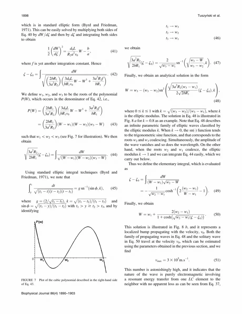
We define w1, w2, and w3 to be the roots of the polynomial

P(W), which occurs in the denominator of Eq. 42, i.e.,

PðWÞ ¼ 2bR1

3a2R2

� �3d0L

bR1v0W �W

31

3a2R2f

bR1

� �

¼ 2bR1

3a2R2

� �ðW � w1ÞðW � w2Þðw3 �WÞ (43)

such that w1\w2\w3 (see Fig. 7 for illustration). We then

obtainffiffiffiffiffiffiffiffiffiffiffiffi3a

2R2

2bR1

sðz� z0Þ ¼

ðdWffiffiffiffiffiffiffiffiffiffiffiffiffiffiffiffiffiffiffiffiffiffiffiffiffiffiffiffiffiffiffiffiffiffiffiffiffiffiffiffiffiffiffiffiffiffiffiffiffiffiffiffiffiffiffi

ðW�w1ÞðW�w2Þðw3�WÞp : (44)

Using standard elliptic integral techniques (Byrd and

Friedman, 1971), we note thatðt1y

dtffiffiffiffiffiffiffiffiffiffiffiffiffiffiffiffiffiffiffiffiffiffiffiffiffiffiffiffiffiffiffiffiffiffiffiffiffiffiffiffiffiffiffiðt1 � tÞðt � t2Þðt � t3Þ

p ¼ g sn�1ðsinf; kÞ; (45)

where g ¼ ð2= ffiffiffiffiffiffiffiffiffiffiffiffiffit1 � t3

p Þ; k ¼ffiffiffiffiffiffiffiffiffiffiffiffiffiffiffiffiffiffiffiffiffiffiffiffiffiffiffiffiffiffiffiffiffiffiffiðt1 � t2Þ=ðt1 � t3Þ

pand

sinf ¼ffiffiffiffiffiffiffiffiffiffiffiffiffiffiffiffiffiffiffiffiffiffiffiffiffiffiffiffiffiffiffiffiffiffiðt1 � yÞ=ðt1 � t2Þ

pwith t1 [ y $ t2 [ t3, and by

identifying

t1 ! w3

t2 ! w2

t3 ! w1 (46)

we obtain

ffiffiffiffiffiffiffiffiffiffiffiffi3a

2R2

2bR1

sðz � z0Þ ¼

2ffiffiffiffiffiffiffiffiffiffiffiffiffiffiffiffiw3 � w1

p sn�1

ffiffiffiffiffiffiffiffiffiffiffiffiffiffiffiffiw3 �W

w3 � w2

r; k

� �: (47)

Finally, we obtain an analytical solution in the form

W ¼ w3 � ðw3 � w2Þsn2ffiffiffiffiffiffiffiffiffiffiffiffiffiffiffiffiffiffiffiffiffiffiffiffiffiffiffiffiffiffiffi3a

2R2ðw3 � w1Þ

q2ffiffiffiffiffiffiffiffiffiffi2bR1

p ðz � z0Þ; k

0@

1A;

(48)

where 0# k# 1 with k ¼ffiffiffiffiffiffiffiffiffiffiffiffiffiffiffiffiffiffiffiffiffiffiffiffiffiffiffiffiffiffiffiffiffiffiffiffiffiffiffiffiffiffiðw3 � w2Þ=ðw3 � w1Þ

p, where k

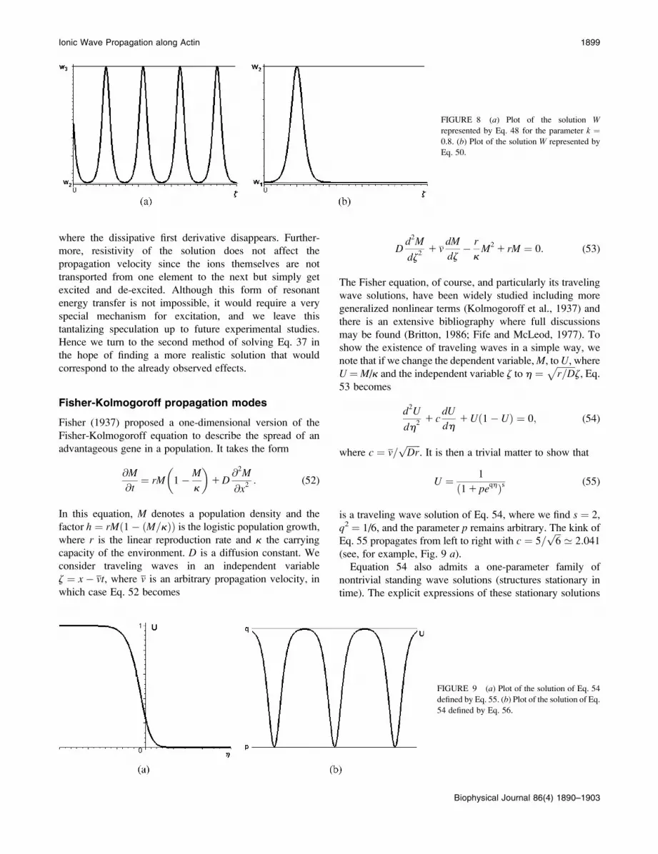
is the elliptic modulus. The solution in Eq. 48 is illustrated in

Fig. 8 a for k¼ 0.8 as an example. Note that Eq. 48 describes

an infinite parametric family of elliptic waves classified by

the elliptic modulus k. When k ! 0, the sn(�) function tends

to the trigonometric sine function, and that corresponds to the

roots w2 and w3 coalescing. Simultaneously, the amplitude of

the wave vanishes and so does the wavelength. On the other

hand, when the roots w2 and w1 coalesce, the elliptic

modulus k ! 1 and we can integrate Eq. 44 easily, which we

carry out below.

Thus we define the elementary integral, which is evaluated

as

z � z0 ¼ð

dW

ðW � w1Þffiffiffiffiffiffiffiffiffiffiffiffiffiffiffiffiw2 �W

p

¼ � 1ffiffiffiffiffiffiffiffiffiffiffiffiffiffiffiffiw2 � w1

p cosh�1

2ðw2 � w1ÞW � w1

� 1

� �: (49)

Finally, we obtain

W ¼ w1 12ðw2 � w1Þ

11 coshffiffiffiffiffiffiffiffiffiffiffiffiffiffiffiffiw2 � w1

p ðz � z0Þ� � : (50)

This solution is illustrated in Fig. 8 b, and it represents a

localized bump propagating with the velocity, v0. Both the

family of propagating waves in Eq. 48 and the solitary wave

in Eq. 50 travel at the velocity v0, which can be estimated

using the parameters obtained in the previous section, and we

find

vmax ¼ 33 105m:s

�1: (51)

This number is astonishingly high, and it indicates that the

nature of the wave is purely electromagnetic involving

a resonant energy transfer from one LC element to the

neighbor with no apparent loss as can be seen from Eq. 37,FIGURE 7 Plot of the cubic polynomial described in the right-hand side

of Eq. 43.



where the dissipative first derivative disappears. Further-

more, resistivity of the solution does not affect the

propagation velocity since the ions themselves are not

transported from one element to the next but simply get

excited and de-excited. Although this form of resonant

energy transfer is not impossible, it would require a very

special mechanism for excitation, and we leave this

tantalizing speculation up to future experimental studies.

Hence we turn to the second method of solving Eq. 37 in

the hope of finding a more realistic solution that would

correspond to the already observed effects.

Fisher-Kolmogoroff propagation modes

Fisher (1937) proposed a one-dimensional version of the

Fisher-Kolmogoroff equation to describe the spread of an

advantageous gene in a population. It takes the form

@M

@t¼ rM 1�M

k

� �1D

@2M

@x2 : (52)

In this equation, M denotes a population density and the

factor h ¼ rMð1� ðM=kÞÞ is the logistic population growth,where r is the linear reproduction rate and k the carrying

capacity of the environment. D is a diffusion constant. We

consider traveling waves in an independent variable

z ¼ x � vt, where v is an arbitrary propagation velocity, in

which case Eq. 52 becomes

Dd2M

dz2 1 v

dM

dz� r

kM2

1 rM ¼ 0: (53)

The Fisher equation, of course, and particularly its traveling

wave solutions, have been widely studied including more

generalized nonlinear terms (Kolmogoroff et al., 1937) and

there is an extensive bibliography where full discussions

may be found (Britton, 1986; Fife and McLeod, 1977). To

show the existence of traveling waves in a simple way, we

note that if we change the dependent variable,M, toU, whereU¼M/k and the independent variable z to h ¼

ffiffiffiffiffiffiffiffir=D

pz, Eq.

53 becomes

d2U

dh2 1 cdU

dh1Uð1� UÞ ¼ 0; (54)

where c ¼ v=ffiffiffiffiffiffiDr

p. It is then a trivial matter to show that

U ¼ 1

ð11 peqhÞs (55)

is a traveling wave solution of Eq. 54, where we find s ¼ 2,

q2 ¼ 1/6, and the parameter p remains arbitrary. The kink of

Eq. 55 propagates from left to right with c ¼ 5=ffiffiffi6

p’ 2:041

(see, for example, Fig. 9 a).Equation 54 also admits a one-parameter family of

nontrivial standing wave solutions (structures stationary in

time). The explicit expressions of these stationary solutions

FIGURE 8 (a) Plot of the solution W

represented by Eq. 48 for the parameter k ¼0.8. (b) Plot of the solution W represented by

Eq. 50.

FIGURE 9 (a) Plot of the solution of Eq. 54

defined by Eq. 55. (b) Plot of the solution of Eq.

54 defined by Eq. 56.



can be obtained in terms of the Jacobian elliptic functions

(see for illustration Fig. 9 b)

UðxÞ ¼ p1 ðq� pÞsn2 1

g

ffiffiffi2

3

rx; k

!; (56)

where p and q are maximum and minimum amplitudes of U,respectively, and g ¼ ð2=

ffiffiffiffiffiffiffiffiffiffiffiffiffiffiffiffiffiffiffiffiffiffiffiffiffi1:5� q� 2p

pÞ (Brazhnik and

Tyson, 1999).

We show, in this section, that the voltage equation, Eq. 37,

may be cast into the Fisher form. To this end, denoting

dV=dz by V9, we write the voltage equation Eq. 37 as

V01 lV91 gV21 dV1 e ¼ 0; (57)

where

l ¼ ðv20 � c2

0a2ÞL

R2a2v0

; g ¼ bR1

a2R2

d ¼ �R1

R2a2 ; e ¼ R1

R2

1

4ba2 �

d0L

R2a2v0

:

To compare the voltage equation with Eq. 53, we must first

linearly transform Eq. 57 to ensure that various parameters

which appear have the correct sign. We define the cor-

responding change of variable as

V ¼ aW1b; (58)

where a and b are constants to be determined. Thus, Eq. 57

is now expressed as follows:

W01lW91gaW21ð2gb1dÞW1

gb2

a

1db

a1

ea¼ 0: (59)

By identifying the coefficients of Eq. 59 with the coefficients

of Eq. 53. we postulateW¼M and determine the constants a

and b to be

a¼�

ffiffiffiffiffiffiffiffiffiffiffiffiffiffiffiffiffid2�4ge

qgk

and b¼�d1

ffiffiffiffiffiffiffiffiffiffiffiffiffiffiffiffiffid2�4ge

q2g

: (60)

Thus the new dependent voltage, W, which is a scaled and

shifted form of the original voltage, V, satisfies a one-

dimensional Fisher equation like that in Eq. 53. Hence the

traveling wave solution described in Eq. 55 can be used to

define the solution V of Eq. 57 as

V ¼ 1

2b1

ffiffiffiffiffiffiffiffiffiffiffid0L

bR1v0

r

3 1� 2

11peq

ffiffiffiffiffiffiffiffiffiffiffiffiffiffiffiffiffiffiffiffiffiffiffiffiffiffiffiffiffiffiffiffiffið2=a2R2Þ

ffiffiffiffiffiffiffiffiffiffiffiffiffiffiffiffiffiðbd0R1L=v0Þ

ppz

� �s

0BB@

1CCA: (61)

It is worth pointing out that all the physical parameters

appear in the mathematical description of the kink. The

capacitance dependence arises from v or vmax. R1, R2, and Ldetermine the shape of the kink such that the amplitude is

proportional toffiffiffiL

pand inversely proportional to

ffiffiffiffiffiR1

pandffiffiffi

bp

. Note that in the limit of the nonlinearity coefficient

b tending to zero, the solution becomes singular and hence

unphysical. The width of the kink is proportional toffiffiffiffiffiR2

pand

the lattice constant a and inversely proportional to the quarticroot of bR1L. We point out that there is a dependence of these

physical parameters on the chemical state of the solution and

the temperature under which experiments are carried out.

The values of the resistance depend on the temperature, the

viscosity, and concentration of the solution. In Fig. 10, we

show the only available experimental data supporting the

presence of soliton waves along actin filament. However, in

FIGURE 10 Experimental plots of (a) the soliton amplitude versus the pulse amplitude, (b) the soliton width versus the pulse voltage, and (c) the number of

solitons generated versus the pulse voltage, following Lin and Cantiello (1993).



view of the presence of only three data points, a quantitative

comparison between our predictions and experiment is not

warranted at present.

Note that the actual propagation velocity for the traveling

kink solution is given by

v ¼ D v2

0� v2

max

� �L

R2a2v0

: (62)

We have established earlier that vmax¼ 33 105m.s�1 and the

values of the remaining constants have also been determined

except for the diffusion constant, D. However, it is well

known that the diffusion constant for ions in aqueous sol-

utions is on the order of 10�9 m2.s�1 (Tuszynski and Dixon,

2001). The velocity parameter, v0, determines the unidirec-

tional flow of the ions, whereas v is the velocity of the moving

nonlinear wave. With the above estimates we find that

v ’ 108ðm:s

�1Þ2

v0: (63)

Interestingly, this indicates that slow linear waves give rise to

fast nonlinear propagation of localized ionic clusters. We

expect that v0 is much less than vmax. With this in mind, and

the knowledge that the velocity of ion flows in physiological

situations, such as action-potential propagation (Alberts

et al., 1998), ranges between 0.1 and 10 m.s�1, we estimate

the corresponding nonlinear wave velocities, v, to be such

that

100m:s�1

$ v$ 1m:s�1: (64)

This study only provides an indication as to a realistic model

of actin that can support soliton-like ionic traveling waves.

Modeling relies on data constrained by experimental

conditions, and/or assumptions made, including the charge

density, which is calculated based on the net surface charges

of actin. It should also be considered that soliton velocity is

directly proportional to the magnitude of the stimulus, which

in a biological setting has not been formally described. Actin

interacts with a number of ion channels, of different ionic

permeability, and conductance. Thus, it is expected that

channel opening, single-channel currents, and other channel

properties, including the resting potential of the cell, may

significantly modify the amplitude and velocity of the

soliton-supported waves. This should correlate with the

velocity of the traveling waves along channel-coupled

filaments. Other parameters that may play a role in this type

of electrodynamic interaction are the local ionic gradients

and the regulatory role of actin-binding proteins, which can

help ‘‘focus’’ the conductive medium or otherwise impair

wave velocity.

CONCLUSIONS

Motivated by several intriguing experiments (Cantiello et al.,

1991; Lin and Cantiello, 1993) that indicated the possibility

of ionic wave generation along actin filaments, we have

developed a physical model that provides a framework for

the analysis of these waves. The background for the model

is the molecular structure of an actin filament and its interac-

tion with solvent ions. Following earlier ideas, we have

represented the filament with the surrounding ions as an

electrical transmission line with L, R, and C elements in it.

One of the key aspects is the nonlinearity of the associated

capacitance (Ma et al., 1999; Wang et al., 1999) that

eventually gives rise to the self-focusing of the ionic waves.

The equations developed for the model originate from the

application of Kirchhoff’s laws to the LRC resonant circuit

of a model actin monomer in a filament. We then took the

continuum limit and determined second order partial

differential equations for the spatio-temporal dependence

of voltage. These nonlinear equations were eventually solved

using two different approaches. The first ansatz resulted in

a zero dissipation state (due to the absence of resistive terms)

corresponding to an absolute maximum velocity of propa-

gation. This, however, implies a purely electromagnetic

disturbance propagating resonantly from node to node in the

circuit. A more physically realistic case involved mapping

our equation onto the Fisher-Kolmogoroff equation with the

attendant elliptic and topological solitonic solutions. The

elliptic waves were stationary in time and may lead to the

establishment of spatial periodic patterns of ionic concen-

tration. Perhaps the most important finding obtained in this

work is the existence of the traveling wave kink, which

describes a moving transition region between a high and low

ionic concentration due to the corresponding intermono-

meric voltage gradient. The velocity of propagation was

estimated to range between 1 and 100 m.s�1, depending on

the characteristic properties of the electrical circuit model. It

is noteworthy that these values overlap with action potential

velocities in excitable tissues (Hille, 1992).

We believe that these findings may have important

consequences for our understanding of the signaling and

ionic transport at intracellular level. Extensive new in-

formation (Janmey, 1998) indicates that actin filaments are

both directly (Chasan et al., 2002) and indirectly linked to

ion channels in both excitable and nonexcitable tissues,

providing a potentially relevant electrical coupling between

these current generators (i.e., channels), and intracellular

transmission lines (i.e., actin filaments). Furthermore, actin

filaments are crucially involved in cell motility and, in this

context, they are known to be able to rearrange their spatial

configuration. It is tantalizing to speculate that ionic waves

surrounding these filaments may participate or even trigger

the rearrangement of intracellular actin networks. In nerve

cells, actin filaments are mainly located in the synaptic

bouton region. Again, it would make sense for electrical

signals supported by actin filaments to help trigger

neurotransmitter release through voltage-modulated mem-

brane deformation leading to exocytosis (Segel and Parnas,

1991). Actin is also prominent in postsynaptic dendritic



spines, and its dynamics within dendritic spines has been

implicated in the postsynaptic response to synaptic trans-

mission. Kaech et al. (1999) have shown that general

anesthetics inhibit this actin-mediated response. Incidentally,

it is noteworthy that Claude Bernard showed also that the

anesthetic gas chloroform inhibited cytoplasmic movement

in slime mold. Actin structural dynamics plays a significant

role in synaptic plasticity and neuronal function. Among

functional roles of actin in neurons, we mention in passing

glutamate receptor channels that are implicated in long-term

potentiation. It is therefore reasonable to expect ionic wave

propagation along actin filaments to lead to a broad range of

physiological effects.

J. M. Dixon thanks the staff and members of the Physics Department of the

University of Alberta for all their kindness and thoughtfulness during his

stay.

This project has been supported by grants from the Natural Sciences and

Engineering Research Council and Mathematics of Information Technology

and Complex Systems. S. Portet acknowledges support from the Bhatia

Post-Doctoral Fellowship Fund.

REFERENCES

Alberts, B., D. Bray, A. Johnson, J. Lewis, M. Raff, K. Roberts, and P.Walter. 1998. Essential Cell Biology: An Introduction to the MolecularBiology of the Cell. Garland Science Publishing, New York.

Anderson, C., and M. Record. 1990. Ion distributions around DNA andother cylindrical polyions: theoretical descriptions and physical implica-tions. Annu. Rev. Biophys. Biophys. Chem. 19:423–465.

Baverstock, K., and R. Cundall. 1988. Solitons and energy transfer in DNA.Nature. 332:312–313.

Brazhnik, P., and J. Tyson. 1999. On traveling wave solutions of Fisher’sequation in two spatial dimensions. SIAM J. Appl. Math. 60:371–391.

Britton, N. 1986. Reaction-Diffusion Equations and Their Applications toBiology. Academic Press, New York.

Byrd, P., and M. Friedman. 1971. Handbook of Elliptic Integrals forEngineers and Scientists. Springer, Berlin.

Cantiello, H., C. Patenande, and K. Zaner. 1991. Osmotically inducedelectrical signals from actin filaments. Biophys. J. 59:1284–1289.

Chasan, B., N. Geisse, K. Pedatella, D. Wooster, M. Teintze, M. Carattino,W. Goldmann, and H. Canteillo. 2002. Evidence for direct interactionbetween actin and the cystic fibrosis transmembrane conductanceregulator. Eur. Biophys. J. 30:617–624.

Coppin, C., and P. Leavis. 1992. Quantitation of liquid-crystalline orderingin F-actin solution. Biophys. J. 63:794–807.

Davydov, A. S. 1982. Biology and Quantum Mechanics. Pergamon Press,Oxford, UK.

Fife, P., and J. McLeod. 1977. The approach of solutions of nonlineardiffusion equations to traveling wave solutions. Arch. Rat. Mech. Anal.65:335–361.

Fisher, R. 1937. The wave of advance of advantageous genes. Ann.Eugenics. 7:353–369.

Frohlich, H. 1975. The extraordinary dielectric properties of biologicalmaterials and the action of enzymes. Proc. Natl. Acad. Sci. USA.72:4211–4215.

Frohlich, H. 1984. Nonlinear Electrodynamics in Biological Systems.Plenum Press, New York.

Furukawa, R., R. Kundra, and M. Fechkeimer. 1993. Formation of liquidcrystals from actin filaments. Biochemistry. 32:12346–12352.

Hagan, S., S. R. Hameroff, and J. A. Tuszynski. 2002. Quantumcomputation in brain microtubules: decoherence and biological feasibil-ity. Phys. Rev. E. 65:1–10.

Hameroff, S., A. Nip, M. Porter, and J. A. Tuszynski. 2002. Conductionpathways in microtubules, biological quantum computation, and con-sciousness. Biosystems. 64:149–168.

Hille, B. 1992. Ionic Channels of Excitable Membranes. SinauerAssociates, Sunderland, MA.

Holmes, K., D. Popp, W. Gebhard, and W. Kabsch. 1990. Atomic model ofthe actin filament. Nature. 347:44–49.

Janmey, P. 1998. The cytoskeleton and the cell signaling: componentlocalization and mechanical coupling. Physiol. Rev. 78:763–781.

Kabsch, W., H. Mannberg, D. Suck, E. Pai, and K. Holmes. 1990. Atomicstructure of the actin: DNAse I complex. Nature. 347:37–44.

Kaech, S., H. Brinkhaus, and A. Matus. 1999. Volatile anesthetics blockactin-based motility in dendritic spines. Proc. Natl. Acad. Sci. USA. 96:10433–10437.

Kobayasi, S. 1964. Effect of electric field on F-actin orientated by flow.Biochim. Biophys. Acta. 88:541–552.

Kobayasi, S., H. Asai, and F. Oosawa. 1964. Electric birefringence of actin.Biochim. Biophys. Acta. 88:528–540.

Kolmogoroff, A., I. Petrovsky, and N. Piscounoff. 1937. Study of thediffusion equation with growth of the quantity of matter and itsapplication to a biological problem. Moscow Univ. Bull. Math. 1:1–25.

Kolosick, J., D. Landt, H. Hsuan, and K. Lonngren. 1974. Properties ofsolitary waves as observed on a non-linear dispersive transmission line.Proc. IEEE. 62:578–581.

Lader, A., H. Woodward, E. Lin, and H. Cantiello. 2000. Modeling of ionicwaves along actin filaments by discrete electrical transmission lines.METMBS ’00 International Conference. 77–82.

Le Bret, M., and B. H. Zimm. 1984. Distribution of counterions arounda cylindrical polyelectrolyte and Manning’s condensation theory.Biopolymers. 23:287–312.

Lin, E., and H. Cantiello. 1993. A novel method to study theelectrodynamic behavior of actin filaments. Evidence of cable-likeproperties of actin. Biophys. J. 65:1371–1378.

Lonngren, K. 1978. Observations of solitons on non-linear dispersivetransmission lines. In Solitons in Action. K. E. Lonngren and A. C. Scotteditors. Academic Press, New York. 127–152.

Ma, Z., J. Wang, and H. Guo. 1999. Weakly nonlinear ac response: theoryand application. Phys. Rev. B. 59:7575–7578.

MacInnes, D. A. 1961. The Principles of Electrochemistry. DoverPublications, London.

Manning, G. 1969. Limiting laws and counterion condensation inpolyelectrolyte solutions I. Colligative properties. J. Chem. Phys.51:924–933.

Manning, G. S. 1978. The molecular theory of polyelectrolyte solutionswith applications to the electrostatic properties of polynucleotides. Q.Rev. Biophys. 2:179–246.

Mavromatos, N. E. 1999. Quantum-mechanical coherence in cell micro-tubules: a realistic possibility? Bioelectrochem. Bioenerg. 48:273–284.

Noguchi, A. 1974. Solitons in a non-linear transmission line. Electronicsand Communications in Japan. 57:9–13.

Oosawa, F. 1970. Counterion fluctuation and dielectric dispersion in linearpolyelectrolytes. Biopolymers. 9:677–688.

Oosawa, F. 1971. Polyelectrolytes. Marcel Dekker, New York.

Ostrovskii, L. 1977. Shock waves and solitons (selected problems).Radiophysics and Quantum Electronics. 18:464–486.

Parodi, M., B. Bianco, and A. Chiabrera. 1985. Toward molecularelectronics. Self-screening of molecular wires. Cell Biophys. 7:215–235.

Pollard, T., and J. Cooper. 1986. Actin and actin-binding proteins. a criticalevaluation of mechanisms and functions. Annu. Rev. Biochem. 55:987–1035.



Rullman, J., and P. van Duijnem. 1990. Potential energy models ofbiological macromolecules: a case ab initio quantum chemistry. Rep.Mol. Theory. 1:1–21.

Sataric, M., J. Tuszynski, and R. Zakula. 1993. Kink-like excitations as anenergy-transfer mechanism in microtubules. Phys. Rev. E. 48:589–597.

Segel, L., and H. Parnas. 1991. What controls the exocytosis of neuro-transmitters. In Biologically Inspired Physics. L. Peliti, editor. PlenumPress, New York.

Sept, D., J. Xu, T. Pollard, and J. McCammon. 1999. Annealing accountsfor the length of actin filaments formed by spontaneous polymerization.Biophys. J. 77:2911–2919.

Tang, J., and P. Janmey. 1996. The polyelectrolyte nature of F-actin andthe mechanism of actin bundle formation. J. Biol. Chem. 271:8556–8563.

Torbet, J., and M. Dickens. 1984. Orientation of muscle actin in strongmagnetic fields. FEBS Lett. 173:403–406.

Tuszynski, J. A., and J. M. Dixon. 2001. Biomedical Applications ofIntroductory Physics. John Wiley and Sons, New York.

Wang, B. G., X. A. Zhao, J. Wang, and H. Guo. 1999. Nonlinear quantumcapacitance. Appl. Phys. Lett. 74:2887–2889.

Zimm, B. 1986. Use of the Poisson-Boltzmann equation to predict ion con-densation around polyelectrolytes. InCoulombic Interactions inMacromo-lecular Systems.A.Gisenhart andF.E.Bailey, editors.AmericanChemicalSociety,Washington, DC. 212–215.



ionic wave propagation along actin filaments

Documents