Investment Returns and Price Discovery

in the

Market for Owner-Occupied Housing∗

by

John M. Quigley†

University of California, Berkeley

Christian L. Redfearn‡

University of Southern California

Abstract

This paper examines the dynamics of owner-occupied housing prices both at thelevel of the individual dwelling and in aggregate. Using a unique data set, a modelof individual dwelling prices is estimated that represents features of housing marketsmore faithfully than competing models. Statistical tests strongly reject the hypothesisthat individual housing prices follow a random walk in favor of the alternative hypoth-esis that housing prices are mean reverting. This result also holds in aggregate, andprovides an explanation for the “inertia” reported in housing return series. The paperthen demonstrates that real and excess returns are forecastable. Finally, it considersempirically the extent to which the transactions costs associated with home ownershippreclude profitable speculation in owner-occupied housing markets.

∗Paper prepared for the Fifth annual conference of the Asian Real Estate Society, July 26-30, 2000. Aprevious revision of this paper was presented at the NBER Workshop on Real Estate Markets, November1999. We are grateful to Owen Lamont and Tom Rothenberg for commentary and discussion.

†quigley@econ.berkeley.edu, phone:1-510-643-7411, fax:1-510-643-7357‡redfearn@econ.berkeley.edu, phone:1-510-643-3507, fax:1-510-643-7357

1

1 Introduction

Many of the features that distinguish owner-occupied housing from other goods imply it is

traded in a specialized and peculiar market. The heterogeneity of housing, its indivisibil-

ity and durability, its fixed location, and the large capital requirement for home purchase

represent substantial deviations from the textbook ideal of the perfect market. Housing is

both a consumption good and a store of wealth, but its market looks neither like conven-

tional goods nor capital markets. Housing markets are decentralized, characterized by high

transactions and search costs, the complete absence of futures markets, and a dearth of

professional traders willing to buy and sell houses in the way equities and commodities are

routinely traded. Given the many frictions associated with housing transactions, it should

be no surprise to find housing price behavior at odds with that predicted by simple models

of housing markets.1 Indeed, since Case and Shiller (1990) reported that both real and ex-

cess returns were forecastable, several other researchers (Guntermann and Norrbin (1991),

Gatzlaff (1994), and Malpezzi (1999), among others) have documented predictable returns

in housing markets, typically by demonstrating that some aggregate price series exhibit “in-

ertia” in returns. However, little is known about the dynamics of individual housing prices

or whether the “inertia” found in aggregate prices has foundations the level of the dwelling.

This paper examines the dynamics of owner-occupied housing markets using a body

of data uniquely suited to this task. The data consist of each and every house sale in

Sweden during a thirteen-year period. We develop a model of housing prices that more

closely represents market features that are specific to housing markets, incorporating a more

general, and more appropriate, structure of prices at the level of the individual dwelling.

This supports a direct test of the hypothesis that individual dwelling prices follow a random

walk against the alternative hypothesis of mean reversion. We then link these results to

movements in aggregate measures of housing prices and their dynamic properties. The model

is more general than other widely-used methods of measuring aggregate housing prices.2 Our

1Grossman and Stiglitz (1980) show that positive information costs alone preclude an informationallyefficient market.

2For example, the “standard method”–used extensively in academic and professional research and reportedby government agencies (i.e., OFHEO)–is shown to be a special case of the model developed below.

2

framework supports explicit tests of the assumptions implicit in the conventional models.

Maximum likelihood results clearly indicate that, at the individual dwelling level, house

prices do not follow a random walk. It is evident that the error variances in prices are an

increasing function of time between sales, but the variances do not conform to the behavior

implied by a random walk. The high, but not perfect, serial correlation in the error structure

at the individual dwelling level implies that changes in aggregate housing prices will also be

serially correlated in a predictable way. The empirical results indicate that shocks to prices

persist over several years, offering a powerful explanation for the observed predictability in

aggregate housing prices.

Finally, the paper addresses whether there exists an investment rule that consistently

yields extra-normal returns, given this understanding of the structure of aggregate returns.

Using data on repeat sales of the same, unchanged, dwelling and standard bootstrap tech-

niques, the value of this information to different economic agents is examined. The results

of this section show that–while returns are somewhat predictable–the institutional struc-

ture of housing markets precludes consistent excess returns. In fact, the simulations suggest

that economic agents in housing markets compete away the excess profits to approximately

the level of the transactions costs of buying and selling housing for the typical participant.

The results should be generalizable to other housing markets–as detailed below, the costs

associated with entry and exit to the markets studied are similar to those in other markets.

Section 2 develops a general model of housing prices that permits an explicit test for a

random walk in individual housing prices. This section demonstrates that a widely employed

method of measuring housing prices, proposed by Bailey, Muth, and Nourse (1963) and

extended by Case and Shiller (1987), is a special case of the general model. The data are

described in Section 3. Section 4 presents a set of empirical results: tests for random walk

in house prices against the alternative of a mean reverting process, and the link between

individual pricing errors and aggregate price movements. Tests for the predictability of

aggregate returns appear in Section 5, as do evaluations of the profitability of plausible

investment rules available to market actors. Section 6 concludes.

3

2 A Simple Model of Housing Prices

Price discovery in housing markets cannot occur as it does in many other contexts. Unlike

routinely purchased goods, housing transacts infrequently. Most other goods can be trans-

ported to the market offering the highest return; this is impossible in the case of housing. The

fixed location of housing implies that even dwellings with identical physical structures may

differ in price simply because the price incorporates a complicated set of site-specific ameni-

ties and costs. Furthermore, the stock of housing is characterized by diversity–dwellings vary

widely across structural attributes, style, and vintage. In short, “comparison shopping” in

housing markets is more problematic than it is in many other goods markets; it is substan-

tially more difficult to determine the market price of a dwelling when every other previously

sold dwelling is necessarily an imperfect substitute.

As a result, housing markets are characterized by a costly process matching heterogeneous

agents on both sides of a transaction involving a heterogeneous good. The expensive and

time-consuming search in which buyers and sellers engage implies that, in housing markets,

sales prices are determined by a small number of participants. Certainly, the observed

sale price of any dwelling may deviate substantially from one that would be obtained if

information in housing markets were costless.

In practice, buyers, sellers, and their agents estimate the “market price” of a home by

utilizing the information embodied in the set of previously sold dwellings. The usefulness

of any one of these sales as a reference depends its similarity across several dimensions:

physical, spatial, and temporal. Because housing trades infrequently, the arrival of new

information about market values is slow. Indeed, from an informational standpoint, the

closest comparable sale across these various dimensions may be the previous sale of the same

dwelling.

The effort to uncover the market value of a dwelling is further complicated by the fact

that an observed sales price is not only a function of market value, but also of unobserved

buyer and seller characteristics (Quan and Quigley 1991). For any given sale, all that is

known is that an offer was received that was higher the owner’s reservation price.

4

The model presented below addresses the price dynamics of housing markets at the level

of the individual dwelling by accounting for two sources of stochastic error. The first is

white noise at the time of sale, reflecting unobserved buyer and seller characteristics in a

thin market. The urgency to purchase on the part of the buyer and the holding costs incurred

by the the seller are two examples of factors that can cause the price of a particular dwelling

to deviate from the price that would be obtained in a thick market, i.e., a market with many

bidders and comparable dwellings for sale.

The second type of pricing error characterizes the price dynamics in housing markets at

the level of the individual dwelling. In a perfect housing market, “errors” in price would

reflect new information about the market’s valuation of the dwelling and would fully and

permanently be incorporated into the dwelling’s price. In this case housing prices would

follow a random walk. In an imperfect market, pricing errors could persist because market

participants either fail to perceive them or lack the ability to exploit them.

Let the log sale price of dwelling i at time t be given by

Vit = Pt + Qit + ξit = Pt + Xitβ + ξit,(1)

where Vit is the log of the observed sales price of dwelling i at time t, Pt is the log of aggregate

housing prices. Qit is the log of housing quality. Housing quality is parameterized by Xit,

the set of relevant dwelling attributes, and β, a vector of coefficients from which implicit

prices can be derived for each attribute. The stochastic component is a composite error,

ξit = εit + ηit,(2)

reflecting the two sources of uncertainty in the model discussed above: that which occurs at

the time of sale, ηit, and that which persists over time, εit. ηit is white-noise, with mean 0

and variance σ2η . As discussed above, the persistence of pricing errors reflects the process by

which the housing market incorporates new information about the market price of a dwelling.

The arrival of new information in the form of other dwelling sales will eventually eliminate

the previous pricing error. We model this persistence as an autocorrelated process:

εit = λεi,t−1 + µit,(3)

5

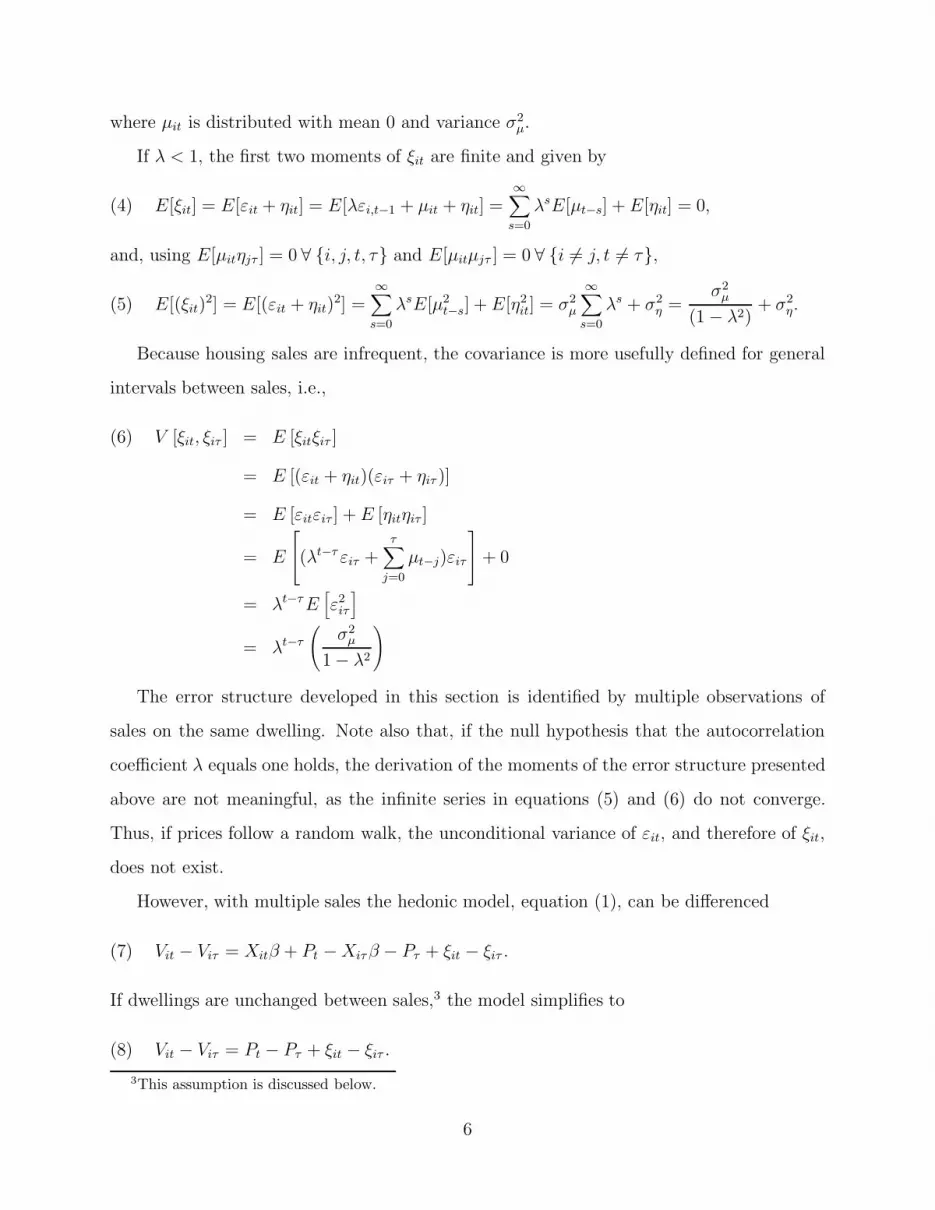
where µit is distributed with mean 0 and variance σ2µ.

If λ < 1, the first two moments of ξit are finite and given by

E[ξit] = E[εit + ηit] = E[λεi,t−1 + µit + ηit] =∞∑

s=0

λsE[µt−s] + E[ηit] = 0,(4)

and, using E[µitηjτ ] = 0 ∀ {i, j, t, τ} and E[µitµjτ ] = 0 ∀ {i 6= j, t 6= τ},

E[(ξit)2] = E[(εit + ηit)

2] =∞∑

s=0

λsE[µ2t−s] + E[η2

it] = σ2µ

∞∑s=0

λs + σ2η =

σ2µ

(1 − λ2)+ σ2

η.(5)

Because housing sales are infrequent, the covariance is more usefully defined for general

intervals between sales, i.e.,

V [ξit, ξiτ ] = E [ξitξiτ ](6)

= E [(εit + ηit)(εiτ + ηiτ )]

= E [εitεiτ ] + E [ηitηiτ ]

= E

(λt−τ εiτ +τ∑

j=0

µt−j)εiτ

+ 0

= λt−τ E[ε2

iτ

]= λt−τ

(σ2

µ

1 − λ2

)

The error structure developed in this section is identified by multiple observations of

sales on the same dwelling. Note also that, if the null hypothesis that the autocorrelation

coefficient λ equals one holds, the derivation of the moments of the error structure presented

above are not meaningful, as the infinite series in equations (5) and (6) do not converge.

Thus, if prices follow a random walk, the unconditional variance of εit, and therefore of ξit,

does not exist.

However, with multiple sales the hedonic model, equation (1), can be differenced

Vit − Viτ = Xitβ + Pt − Xiτβ − Pτ + ξit − ξiτ .(7)

If dwellings are unchanged between sales,3 the model simplifies to

Vit − Viτ = Pt − Pτ + ξit − ξiτ .(8)

3This assumption is discussed below.

6

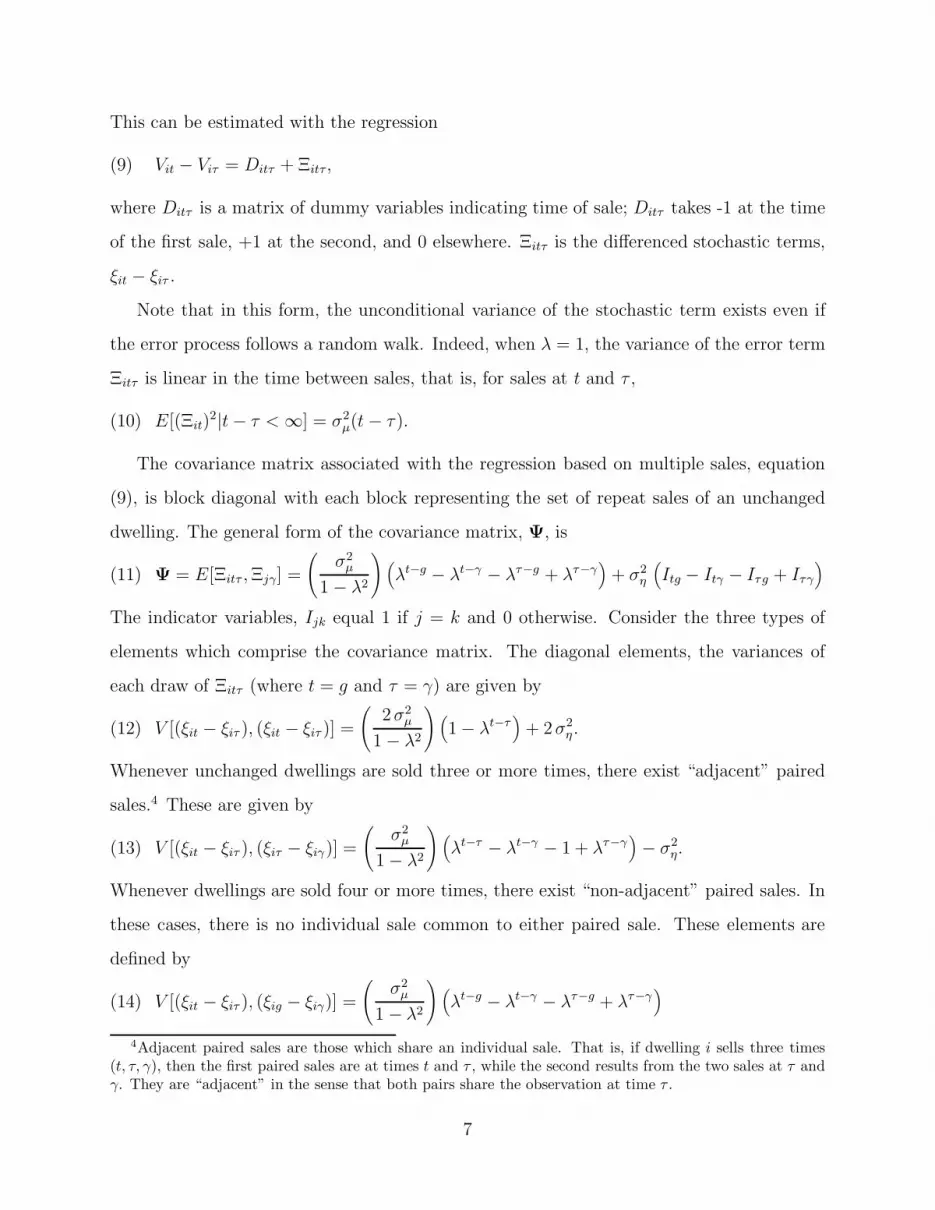
This can be estimated with the regression

Vit − Viτ = Ditτ + Ξitτ ,(9)

where Ditτ is a matrix of dummy variables indicating time of sale; Ditτ takes -1 at the time

of the first sale, +1 at the second, and 0 elsewhere. Ξitτ is the differenced stochastic terms,

ξit − ξiτ .

Note that in this form, the unconditional variance of the stochastic term exists even if

the error process follows a random walk. Indeed, when λ = 1, the variance of the error term

Ξitτ is linear in the time between sales, that is, for sales at t and τ ,

E[(Ξit)2|t− τ < ∞] = σ2

µ(t − τ ).(10)

The covariance matrix associated with the regression based on multiple sales, equation

(9), is block diagonal with each block representing the set of repeat sales of an unchanged

dwelling. The general form of the covariance matrix, Ψ, is

Ψ = E[Ξitτ , Ξjγ] =

(σ2

µ

1 − λ2

)(λt−g − λt−γ − λτ−g + λτ−γ

)+ σ2

η

(Itg − Itγ − Iτg + Iτγ

)(11)

The indicator variables, Ijk equal 1 if j = k and 0 otherwise. Consider the three types of

elements which comprise the covariance matrix. The diagonal elements, the variances of

each draw of Ξitτ (where t = g and τ = γ) are given by

V [(ξit − ξiτ ), (ξit − ξiτ )] =

(2σ2

µ

1 − λ2

)(1 − λt−τ

)+ 2σ2

η .(12)

Whenever unchanged dwellings are sold three or more times, there exist “adjacent” paired

sales.4 These are given by

V [(ξit − ξiτ ), (ξiτ − ξiγ)] =

(σ2

µ

1 − λ2

)(λt−τ − λt−γ − 1 + λτ−γ

)− σ2

η.(13)

Whenever dwellings are sold four or more times, there exist “non-adjacent” paired sales. In

these cases, there is no individual sale common to either paired sale. These elements are

defined by

V [(ξit − ξiτ ), (ξig − ξiγ)] =

(σ2

µ

1 − λ2

)(λt−g − λt−γ − λτ−g + λτ−γ

)(14)

4Adjacent paired sales are those which share an individual sale. That is, if dwelling i sells three times(t, τ, γ), then the first paired sales are at times t and τ , while the second results from the two sales at τ andγ. They are “adjacent” in the sense that both pairs share the observation at time τ .

7

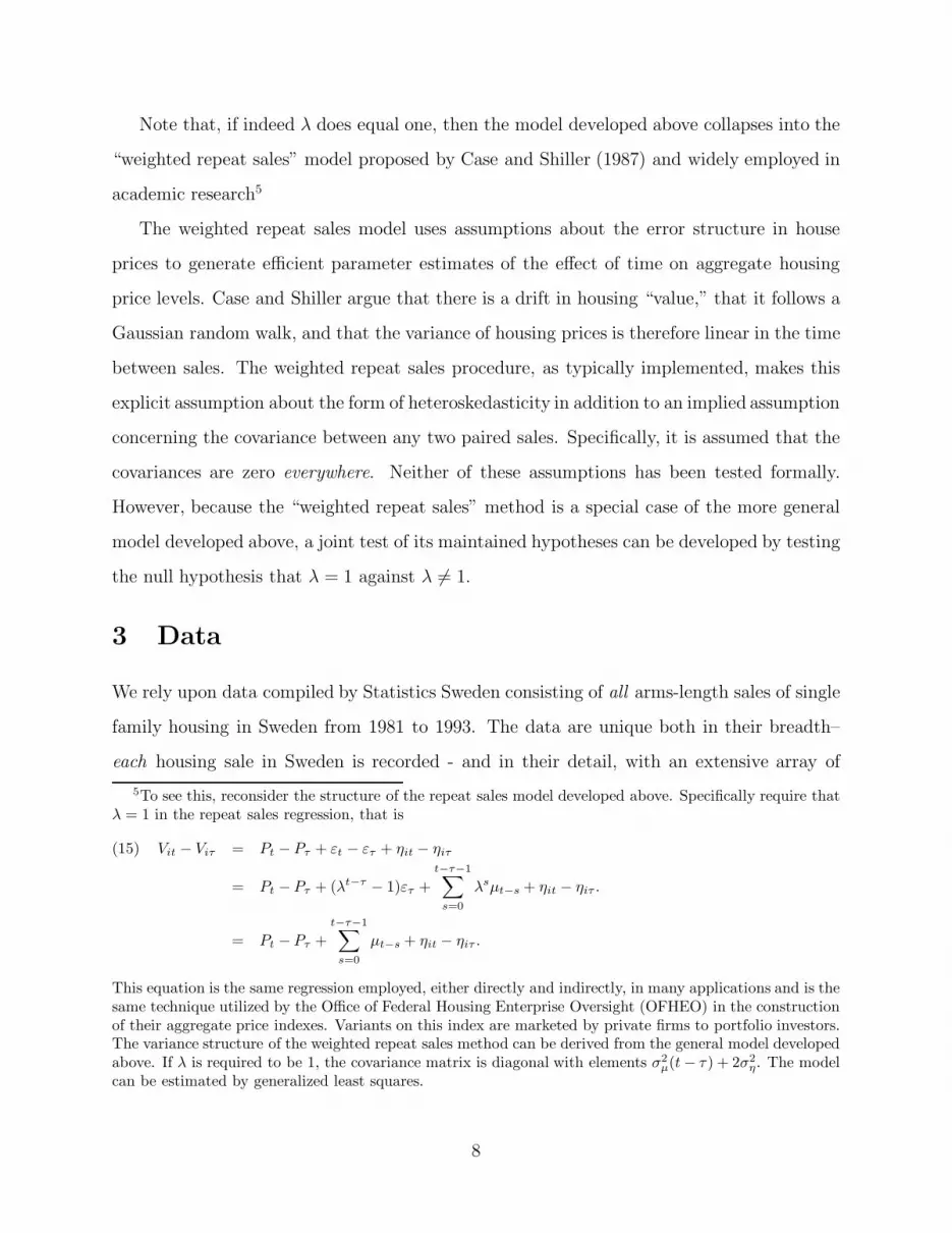
Note that, if indeed λ does equal one, then the model developed above collapses into the

“weighted repeat sales” model proposed by Case and Shiller (1987) and widely employed in

academic research5

The weighted repeat sales model uses assumptions about the error structure in house

prices to generate efficient parameter estimates of the effect of time on aggregate housing

price levels. Case and Shiller argue that there is a drift in housing “value,” that it follows a

Gaussian random walk, and that the variance of housing prices is therefore linear in the time

between sales. The weighted repeat sales procedure, as typically implemented, makes this

explicit assumption about the form of heteroskedasticity in addition to an implied assumption

concerning the covariance between any two paired sales. Specifically, it is assumed that the

covariances are zero everywhere. Neither of these assumptions has been tested formally.

However, because the “weighted repeat sales” method is a special case of the more general

model developed above, a joint test of its maintained hypotheses can be developed by testing

the null hypothesis that λ = 1 against λ 6= 1.

3 Data

We rely upon data compiled by Statistics Sweden consisting of all arms-length sales of single

family housing in Sweden from 1981 to 1993. The data are unique both in their breadth–

each housing sale in Sweden is recorded - and in their detail, with an extensive array of

5To see this, reconsider the structure of the repeat sales model developed above. Specifically require thatλ = 1 in the repeat sales regression, that is

Vit − Viτ = Pt − Pτ + εt − ετ + ηit − ηiτ(15)

= Pt − Pτ + (λt−τ − 1)ετ +t−τ−1∑

s=0

λsµt−s + ηit − ηiτ .

= Pt − Pτ +t−τ−1∑

s=0

µt−s + ηit − ηiτ .

This equation is the same regression employed, either directly and indirectly, in many applications and is thesame technique utilized by the Office of Federal Housing Enterprise Oversight (OFHEO) in the constructionof their aggregate price indexes. Variants on this index are marketed by private firms to portfolio investors.The variance structure of the weighted repeat sales method can be derived from the general model developedabove. If λ is required to be 1, the covariance matrix is diagonal with elements σ2

µ(t − τ ) + 2σ2η. The model

can be estimated by generalized least squares.

8

physical characteristics reported. The research reported below distinguishes among eight

administrative regions—four metropolitan regions (Gothenburg, Malmo, Stockholm, and

Uppsala) and four non-metropolitan regions (the South, the Central, the North, and the Far

North). The data are discussed at length in Englund, Quigley, and Redfearn (1998), but

several features of the data central to this analysis warrant discussion.

First, the detailed set of characteristics that describe the physical structure make it

possible to verify the central assumption of repeat sales models of housing prices, which

is that twice-sold dwellings are identical in attributes at each time of sale. In practice,

this assumption is difficult to verify, but the attributes reported in the data set make this

possible. The data contain not only primary characteristics such as lot size and living area,

but also additional variables that offer a comprehensive description of the dwelling, including

the number of garages, kitchen quality, type of wall, roof, and floor, and the presence of

amenities such as sauna, fireplace, and furnished basement. The list is extensive—in excess

of thirty housing characteristics. This level of detail facilitates the detection of structural

changes that would violate the assumption of constant quality.6 The research reported here

uses only those repeat sales of homes whose measured characteristics are unchanged between

the first and the second sales.

Second, the population of dwellings is a panel so that units that sold more than once

can be distinguished from those that did not. The panel nature of the data identifies the

appropriate specification of the model developed in Section 2.

Table 1 previews the central empirical question addressed in this paper: the relationship

between the length of the time between sales and the distribution of prices. The table shows

the average and standard deviation of the total return from price appreciation for dwellings

on which there are two or more observed sales. Both statistics exhibit strong tendencies to

decline as the number of sales increases. Of course, the average time between sales declines

with the number of sales, since the sample period is fixed. Because the majority of the sales

during the sample period are drawn from a period of rising nominal housing prices, it is not

6Englund, Quigley, and Redfearn (1999a) examine in detail the validity of the constant quality assumption.They find that is does not hold in general, and that failure exclude altered dwellings can lead to substantialbias in measured aggregate house prices.

9

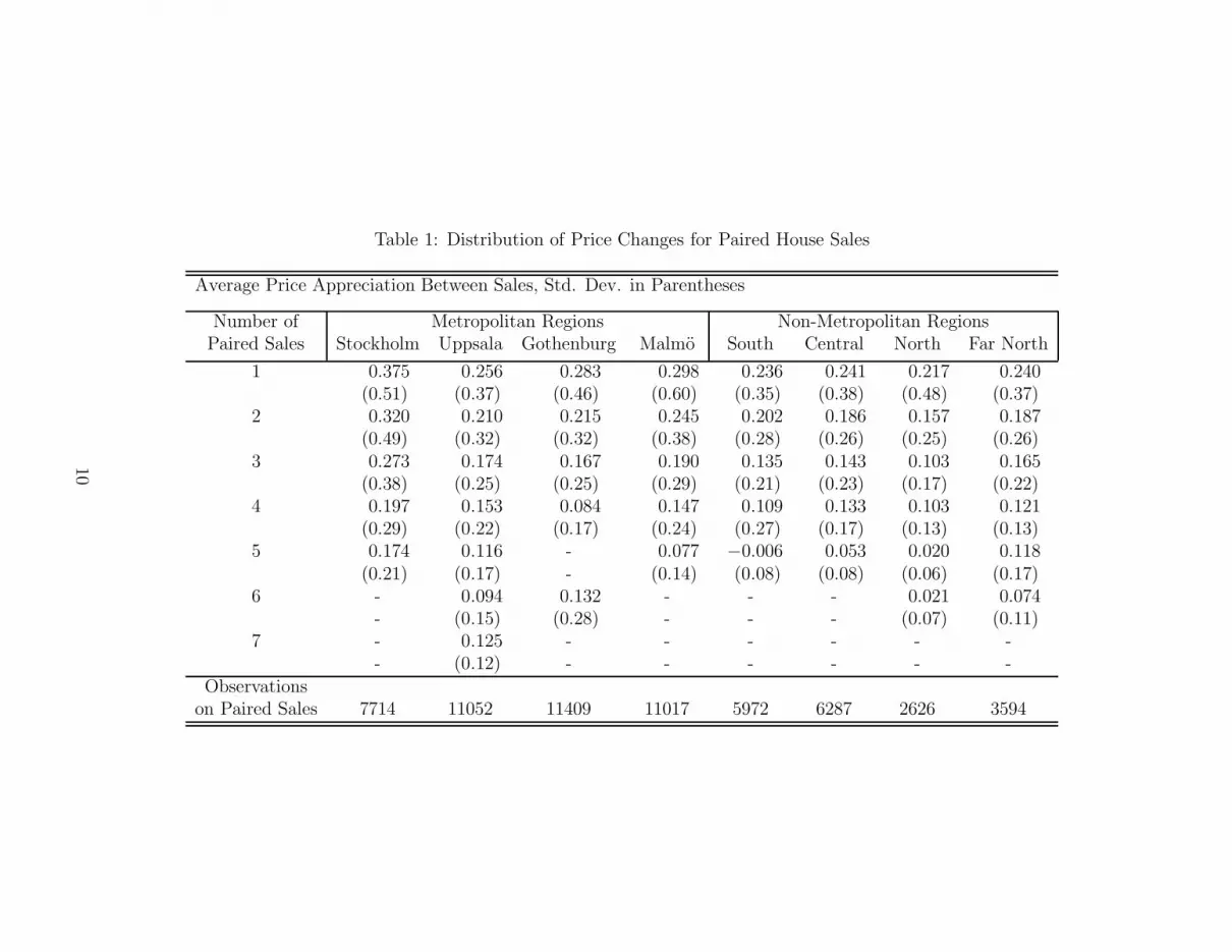
Table 1: Distribution of Price Changes for Paired House Sales

Average Price Appreciation Between Sales, Std. Dev. in Parentheses

Number of Metropolitan Regions Non-Metropolitan RegionsPaired Sales Stockholm Uppsala Gothenburg Malmo South Central North Far North

1 0.375 0.256 0.283 0.298 0.236 0.241 0.217 0.240(0.51) (0.37) (0.46) (0.60) (0.35) (0.38) (0.48) (0.37)

2 0.320 0.210 0.215 0.245 0.202 0.186 0.157 0.187(0.49) (0.32) (0.32) (0.38) (0.28) (0.26) (0.25) (0.26)

3 0.273 0.174 0.167 0.190 0.135 0.143 0.103 0.165(0.38) (0.25) (0.25) (0.29) (0.21) (0.23) (0.17) (0.22)

4 0.197 0.153 0.084 0.147 0.109 0.133 0.103 0.121(0.29) (0.22) (0.17) (0.24) (0.27) (0.17) (0.13) (0.13)

5 0.174 0.116 - 0.077 −0.006 0.053 0.020 0.118(0.21) (0.17) - (0.14) (0.08) (0.08) (0.06) (0.17)

6 - 0.094 0.132 - - - 0.021 0.074- (0.15) (0.28) - - - (0.07) (0.11)

7 - 0.125 - - - - - -- (0.12) - - - - - -

Observationson Paired Sales 7714 11052 11409 11017 5972 6287 2626 3594

10

surprising that total appreciation is higher when the average time between sales is longer.

However, the standard deviation of price appreciation shows consistent reduction in the

volatility in prices between sales as the interval between sales decreases. This is consistent

with the hypothesis that heteroskadasticity in housing price appreciation is a function of the

time interval between sales of the same dwelling.

4 Do House Prices Follow a Random Walk?

The model presented above supports an explicit test the hypothesis that individual housing

prices follow a random walk against the alternative hypothesis that prices follow a mean

reverting process. The test is implemented by maximizing the concentrated log-likelihood

function

logL = −n ∗ (e′glsΨ egls) − det|Ψ|,(16)

where n is the number of observations and egls is the vector of residuals from a generalized

least squares regression. Ψ is the estimated covariance matrix described by (11), a function

of λ. Well-defined probabilistic statements about λ can be made using likelihood-ratio tests.

As discussed in Section 2, the covariance matrix, defined in (11), is block diagonal with

the dimension of each block determined by the number of sales of an unchanged dwelling.

The elements of the covariance matrix depend on the time between sales, the value λ, and

the variances of the pricing errors defined in (1), σ2µ and σ2

η. Consistent estimates of these

error variances are obtained from the regression

eitτeigγ =

2σ2η + h(t, τ, g, γ)σ2

µ if t=g, τ = γ (diagonal elements),

−1σ2η + h(t, τ, g, γ)σ2

µ if τ = g, (off-diagonal elements),

0σ2η + h(t, τ, g, γ)σ2

µ otherwise (off-off diagonal elements).

(17)

The dependent variables, eitτ and eigγ are obtained from the appropriate elements of the outer

product e · e′, where e is the vector of residuals from a first-step regression. h(t, τ, g, γ) is an

element of the covariance matrix, given by (11), defining the expected covariance between

two paired sales of the same dwelling. σ2η and σ2

µ are the estimated regression coefficients.

11

The value of λ that maximizes the log-likelihood function, λ, is easily obtained from this

procedure, as is the value of the log-likelihood function for other values of λ.

Figure 1 illustrates the nature of the maximization problem for one of the metropolitan

areas. The upper panel shows the sample error variances and the relative frequency of

observations by elapsed time, in quarter years, between sales. Two things are clear from

this panel. First, the error variances are an increasing function of the time interval between

sales. Second, the large majority of observations are paired sales in an interval shorter than

than six years. The very high sample variances observed in the longer intervals are based on

small numbers of observations.

The covariance matrix described in (11) defines the predicted variance of the price ap-

preciation as a function of two variables: the elapsed time between sales and the correlation

of the errors. This relationship is illustrated in the lower panel of Figure 1. It again plots

the sample error variances shown in the upper panel, but also the predicted variances using

several assumed values of λ.

Clearly, the three lines with positive serial correlation fit the data far better than does

the line implied by no serial correlation. For a random walk, the variance is linear in the

elapsed time between sales; this would occur if the market permanently incorporated pricing

innovations.

The lines representing intermediate values of serial correlation increase asymptotically to

a level given by the standard definition of the (unconditional) variance of an autocorrelated

process. That is, if the errors follow (3), and |λ| < 1, then

E[(εit)2] =

σ2µ

(1 − λ2).(18)

This implies that for any paired sale, the unconditional variance of price appreciation in-

creases with the correlation coefficient. That is, pricing errors for a particular dwelling

persists as a function of the arrival and incorporation of new information about housing

prices.

Results of the estimation procedure for the both metropolitan and non-metropolitan

regions are plotted in Figure 2. The results offer strong visual support against the random

12

Figure 1:

5 10 15 20 25 30 35 40 45 500

0.05

0.1

0.15

0.2

0.25Sample Variance as a Function of Time Between Sales − Gothenburg

Time Between Sales

Var

ianc

e

Sample variance relative frequency of observations

5 10 15 20 25 30 35 40 45 500

0.05

0.1

0.15

0.2

0.25Predicted Variance as a Function of Time Between Sales and Correlation Coefficient

Time Between Sales

Var

ianc

e

Sample Variancelambda = 0.00 lambda = 0.85 lambda = 0.95 lambda = 1.00

13

Figure 2: Normalized Likelihood Functions for the Eight Regions

0.9 0.91 0.92 0.93 0.94 0.95 0.96 0.97 0.98 0.99 1−1.005

−1.0045

−1.004

−1.0035

−1.003

−1.0025

−1.002

−1.0015

−1.001

−1.0005

−1

lambda

norm

aliz

ed li

kelih

ood

Metropolitan Regions

Stockholm Uppsala GothenburgMalmo

0.9 0.91 0.92 0.93 0.94 0.95 0.96 0.97 0.98 0.99 1−1.015

−1.01

−1.005

−1

lambda

norm

aliz

ed li

kelih

ood

Non−Metropolitan Regions

South Central North Far North

14

Table 2: Tests for a Random Walk in Housing Prices

95% confidence interval

Region λ Lower Bound Upper BoundStockholm 0.933 0.923 0.944Uppsala 0.969 0.962 0.974Gothenburg 0.941 0.933 0.949Malmo 0.962 0.951 0.969South 0.951 0.941 0.962Central 0.964 0.954 0.974North 1.000 0.992 1.000Far North 0.972 0.962 0.982

walk, with λ apparently less than 1 in all but one region. (Time is measured in quarter-year

intervals.)

Formal tests of these conclusions are reported in Table 2. For seven of the eight regions

the upper bound of the 95 percent confidence interval does not include 1. For these seven,

the maximum likelihood value of λ ranges from 0.93 to 0.97. These values suggest that

the housing market removes pricing errors only quite slowly. A quarterly serial correlation

coefficient of 0.95 implies that the market will eliminate only one-fifth of a prior pricing error

over the course of year. That is, after three years just over half of the initial discrepancy

will remain. The discrepancy will not be reduced to ten percent of its initial value for

approximately ten years.

It is straightforward to consider the effect of these individual lags upon aggregate mea-

sures of housing prices. Consider an economy of identical and unchanging dwellings. Let

housing quality be normalized to one so that the log of quality, Xitβ, is zero for all i and

t. Let an estimate of the housing price level be the mean price of the dwellings sold in each

period. That is, let

Pt = n−1∑

i

Vit = n−1

(∑i

Pt +∑

i

εit +∑

i

ηit

)(19)

15

The true housing price index, Pt, is a constant and the mean of the white-noise errors, ηit,

is zero. Denote the average of the the autocorrelated errors as

εt = n−1∑

i

εit.(20)

The estimator of aggregate prices is

Pt = Pt + εt.(21)

The unconditional expectation of Pt is unbiased, since E [εt] = 0. However, with an aggregate

shock to prices one period earlier, εt−1 = e > 0, the aggregate price estimator is no longer

unbiased. The mismeasurement is

Pt = Pt + εt = Pt + λεt−1 = Pt + λe.(22)

Moreover, aggregate pricing errors will lead to correlations in aggregate returns to housing

for many periods if, as indicated above, λ is close to one.

“Inertia” in aggregate prices has become an accepted empirical regularity in housing

markets. Case and Shiller (1990) argue that the predictability in housing returns arises from

the failure of housing markets to incorporate predictable interest rates over the course of their

sample period. Gatzlaff (1994) finds that forecastability is substantially reduced, but not

eliminated, if anticipated inflation is controlled for. Thus, predictable fundamentals may not

be incorporated efficiently into prices. However, the results presented in this section suggest

that persistence at the individual dwelling level can cause persistence at the aggregate level.

If household expectations about housing prices are adaptive, unexpected shocks to housing

prices can lead to predictable changes in aggregate housing prices because the market slowly

incorporates information about the shock. This also accounts for the empirical regularity

that housing returns are correlated.

5 The Predictability of the Returns to Housing

This section examines housing market price dynamics in two ways. First, it tests formally

the proposition that aggregate returns are forecastable. Previous research has found that

16

both real and excess returns are predictable. The results presented here confirm this but

use a more appropriate data set and technique to conduct the tests. The relevant question,

however, is not whether returns are predictable, but rather whether there is a strategy that

consistently realizes excess profits. The second half of the section focuses on this question

using simulations in which the costs of entry and exit are explicitly considered for several

different economic agents.

5.1 Aggregate Returns

The first series considered is the nominal return due to capital appreciation in house prices.

Price appreciation, πt, is simply

πt =Pt

Pt−1− 1,(23)

where Pt is the index of aggregate housing prices.

The second series is real returns, which includes not only the return due to price appre-

ciation but also the “dividend” from the implicit rent paid to owner-occupiers. This total

return is discounted by the change in cost of living index (less shelter). The real return at

time t, rt, is given by

rt =Pt + Rt

Pt−1− CPIt

CPIt−1,(24)

where Rt and CPIt are,respectively, the implicit rent and cost of living indexes at time t.

The aggregate housing price index employed in this section is constructed using the

hybrid model developed in our companion paper, Englund, Quigley, and Redfearn (1998).

The hybrid method uses all available sales information to construct the aggregate price index.

Not only are the large majority of housing transactions during the sample period single sales,

many of those which do sell more than once are altered between sales and, for the purposes

of measuring aggregate prices, are no longer considered repeat sales. The usable data sets

differ by approximately a factor of five for the Swedish data used in this paper.7

7Sample selectivity is also a problem in the repeat sales data sets. Gatzlaff and Haurin (1997), Gatzlaffand Haurin (1998), and Englund, Quigley, and Redfearn (1999a) find that the sample of sold dwellingsare not a random sample of all dwellings and that the appreciation rates of those homes selected into theobserved sample is not reflective of the stock as a whole.

17

Moreover, the appropriate approach for testing the predictability of returns is to approx-

imate, as closely as possible, the information set available to the investor at each point in

time. The small sample problems inherent in repeat sales models are exacerbated over short

intervals.8 In order to avoid this problem, typically the aggregate housing price index is esti-

mated for the entire sample period and it is assumed that investors observe prices only up to

the time period of their decision. However, this approach does not address the fact that the

indexes are conditional on all repeat sales over the entire sample period. This means that

when forecasting changes forward from time t, the estimated price index is calculated using

sales information from t+1 on. The repeat sales indexes used to evaluate the forecastability

of housing returns are, in fact, not the indexes available to agents at time t.

If there were sufficient observations, repeat sales indexes, and the returns series dependent

on them, could be estimated at each point in time. In general, the small fraction of sales

that are repeats precludes period-by-period estimation. Use of the hybrid method avoids this

problem. It is possible, using the Swedish data described above, to estimate an aggregate

price index and each of the returns defined above at each point in time, accurately reflecting

the information available when the housing investment decision is made. Figure 3 plots

the last eight quarters of aggregate price indexes estimated quarter by quarter from 1982:I

forward using the hybrid method. Despite the fact that the hybrid method is substantially

less vulnerable to ex post revisions, the figure shows that the estimated indexes do not take

the same value at the time of estimation as they do when taken from an estimated index

that spans the sample period.

Calculation of the real return series requires an estimate of the implicit rent that accrues

to owners who live in their home. 9

8This problem is discussed and measured in Englund, Quigley, and Redfearn (1999b). They find theconfidence interval around measured prices is vastly larger for the repeat sales method when compared withthose of the hybrid method.

9Previous research has employed local rent indexes as a proxy for the implicit rents, but this is lessappropriate in the Swedish context. The rental market is highly regulated; rents are based on constructioncosts rather than on supply and demand in spot markets. Moreover, at the regulated price, rental marketsdo not clear: there are lengthy waits for apartments in Stockholm. Instead, the proxy used in this researchis obtained by assuming that the implicit rent is equated to the real return on the value of the home.

18

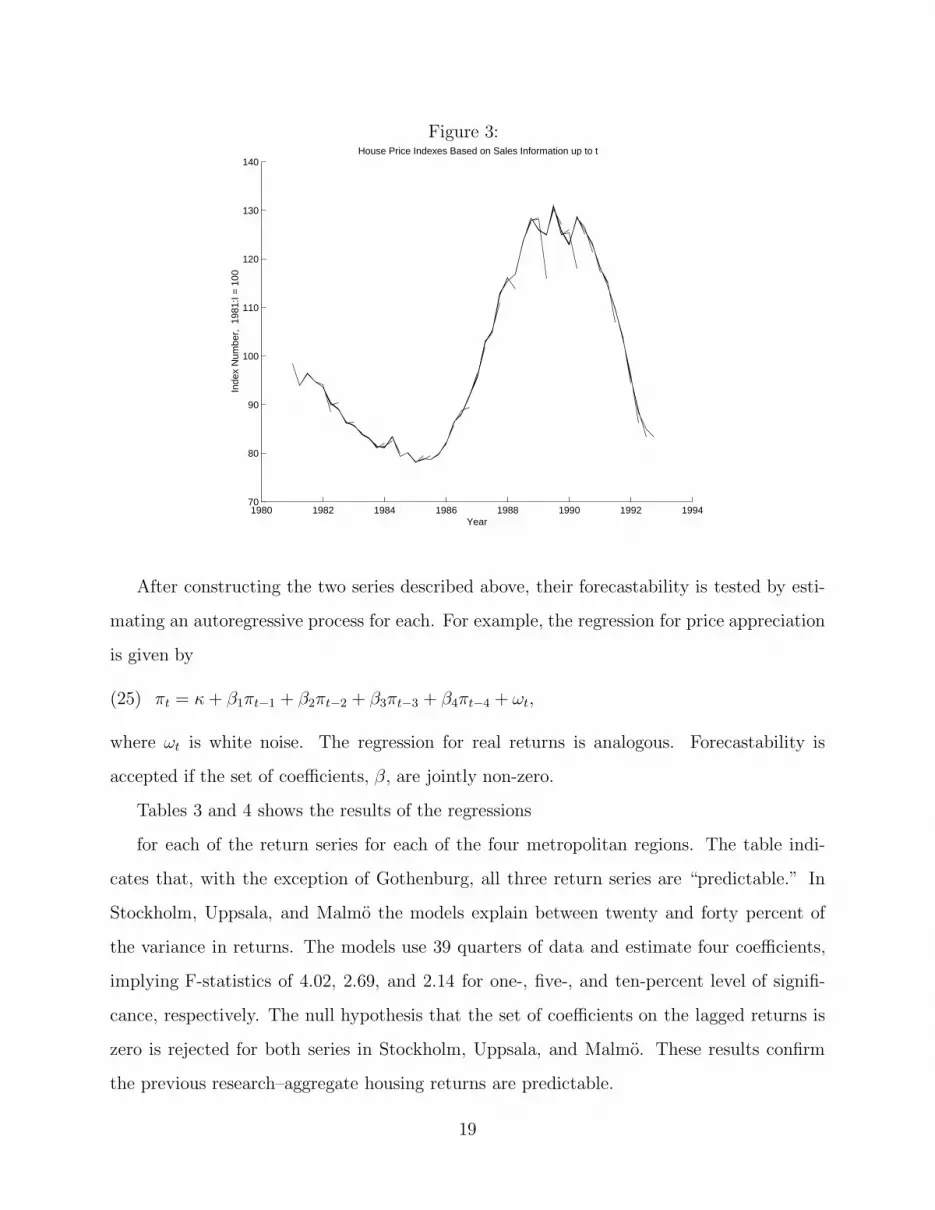
Figure 3:

1980 1982 1984 1986 1988 1990 1992 199470

80

90

100

110

120

130

140

Year

Inde

x N

umbe

r, 1

981:

I = 1

00

House Price Indexes Based on Sales Information up to t

After constructing the two series described above, their forecastability is tested by esti-

mating an autoregressive process for each. For example, the regression for price appreciation

is given by

πt = κ + β1πt−1 + β2πt−2 + β3πt−3 + β4πt−4 + ωt,(25)

where ωt is white noise. The regression for real returns is analogous. Forecastability is

accepted if the set of coefficients, β, are jointly non-zero.

Tables 3 and 4 shows the results of the regressions

for each of the return series for each of the four metropolitan regions. The table indi-

cates that, with the exception of Gothenburg, all three return series are “predictable.” In

Stockholm, Uppsala, and Malmo the models explain between twenty and forty percent of

the variance in returns. The models use 39 quarters of data and estimate four coefficients,

implying F-statistics of 4.02, 2.69, and 2.14 for one-, five-, and ten-percent level of signifi-

cance, respectively. The null hypothesis that the set of coefficients on the lagged returns is

zero is rejected for both series in Stockholm, Uppsala, and Malmo. These results confirm

the previous research–aggregate housing returns are predictable.

19

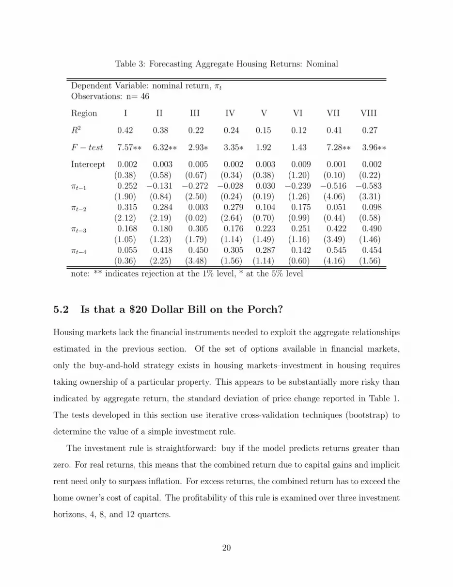
Table 3: Forecasting Aggregate Housing Returns: Nominal

Dependent Variable: nominal return, πt

Observations: n= 46

Region I II III IV V VI VII VIII

R2 0.42 0.38 0.22 0.24 0.15 0.12 0.41 0.27

F − test 7.57∗∗ 6.32∗∗ 2.93∗ 3.35∗ 1.92 1.43 7.28∗∗ 3.96∗∗Intercept 0.002 0.003 0.005 0.002 0.003 0.009 0.001 0.002

(0.38) (0.58) (0.67) (0.34) (0.38) (1.20) (0.10) (0.22)πt−1 0.252 −0.131 −0.272 −0.028 0.030 −0.239 −0.516 −0.583

(1.90) (0.84) (2.50) (0.24) (0.19) (1.26) (4.06) (3.31)πt−2 0.315 0.284 0.003 0.279 0.104 0.175 0.051 0.098

(2.12) (2.19) (0.02) (2.64) (0.70) (0.99) (0.44) (0.58)πt−3 0.168 0.180 0.305 0.176 0.223 0.251 0.422 0.490

(1.05) (1.23) (1.79) (1.14) (1.49) (1.16) (3.49) (1.46)πt−4 0.055 0.418 0.450 0.305 0.287 0.142 0.545 0.454

(0.36) (2.25) (3.48) (1.56) (1.14) (0.60) (4.16) (1.56)

note: ** indicates rejection at the 1% level, * at the 5% level

5.2 Is that a $20 Dollar Bill on the Porch?

Housing markets lack the financial instruments needed to exploit the aggregate relationships

estimated in the previous section. Of the set of options available in financial markets,

only the buy-and-hold strategy exists in housing markets–investment in housing requires

taking ownership of a particular property. This appears to be substantially more risky than

indicated by aggregate return, the standard deviation of price change reported in Table 1.

The tests developed in this section use iterative cross-validation techniques (bootstrap) to

determine the value of a simple investment rule.

The investment rule is straightforward: buy if the model predicts returns greater than

zero. For real returns, this means that the combined return due to capital gains and implicit

rent need only to surpass inflation. For excess returns, the combined return has to exceed the

home owner’s cost of capital. The profitability of this rule is examined over three investment

horizons, 4, 8, and 12 quarters.

20

Table 4: Forecasting Aggregate Housing Returns: Real

Dependent Variable: real return, rt

Observations: n= 46

Region I II III IV V VI VII VIII

R2 0.45 0.38 0.23 0.27 0.16 0.18 0.44 0.27

F − test 8.70∗∗ 6.36∗∗ 3.06∗ 3.81∗ 1.98 2.24 8.19∗∗ 3.85∗∗Intercept −0.002 −0.001 −0.004 −0.003 −0.003 −0.002 −0.008 −0.007

(0.41) (0.33) (0.71) (0.56) (0.69) (0.33) (1.55) (1.05)rt−1 0.175 −0.230 −0.315 −0.034 0.002 −0.330 −0.586 −0.615

(1.26) (1.50) (2.78) (0.28) (0.01) (1.83) (4.43) (3.83)rt−2 0.238 0.210 0.018 0.307 0.094 0.154 0.028 0.101

(1.77) (1.44) (0.12) (2.62) (0.61) (0.98) (0.22) (0.67)rt−3 0.245 0.290 0.343 0.197 0.285 0.360 0.466 0.477

(1.59) (1.82) (2.11) (1.33) (1.93) (1.77) (4.01) (1.45)rt−4 0.187 0.488 0.406 0.296 0.256 0.193 0.535 0.421

(1.42) (3.18) (2.88) (1.43) (1.16) (0.79) (3.99) (1.47)

note: ** indicates rejection at the 1% level, * at the 5% level

The relationship between past and future returns is estimated by exploiting the panel

nature of the data. For each paired sale, both the lagged aggregate returns and realized

return for that particular dwelling are known. Those paired sales which are sold 4, 8, and 12

quarters apart are extracted from the repeat sales data described above. These observations

are then merged with lagged aggregate real and excess returns. The subsample is split–

ninety percent of the merged data are used to estimated the relationship between lagged

returns and realized returns, ten percent is used to test for excess profitability given this

relationship.

For each of the test intervals, the quarterly geometric mean of realized returns in the

ninety-percent subsample are regressed on lagged returns to test for predictability over a

specific investment horizon. The investment rule can then be evaluated. For each of the

remaining observations in the ten-percent subsample–those not used in the regression–the

forecasted return is calculated. If the predicted return is greater than zero, the dwelling

is “purchased.” Realized returns for “purchased” properties are then compared with those

21

which are not.

The number of observations in any one interval is in the hundreds so that the 90/10

split leaves few observations on which to judge profitability. To overcome this problem, the

cross-validation technique just described is repeated. Fifty iterations are executed for each

interval for each of the four regions. The results of this process are displayed in several tables

below.

Table 5 shows the distribution of forecasts for real and excess returns. It contains the

number of sampled dwellings that are forecast to have positive and non-positive returns

and the actual return observed over the period between the two sales. It is immediately

clear that the combined return due to capital gains and implicit rent exceeded inflation for

most of the sample period as almost every sampled dwelling is forecast to have positive real

returns. This is not true of the forecasted excess returns. While a clear majority of sampled

dwellings is forecast to have positive returns, a sizeable minority is not. The difference in

realized excess returns is striking. The average excess return is one to three percentage

points higher per quarter. This indicates that the predictable relationship observed at the

aggregate level holds when measured at the level of the individual dwelling.

However, predictability alone does not indicate the existence of arbitrage opportunities.

In order to determine the potential to exploit the relationship between past and future

returns, it is necessary to account for the substantial costs of buying, owning, and selling

housing. These costs are explained in detail in Soderberg (1995). Table 6 summarizes the

major costs of participating in the housing market for four hypothetical home buyers.

The first is referred to as a market timer. This individual faces no transaction costs as

they are considered sunk costs–he is living at home with his parents and waiting for the

right time to buy. The second buyer is the mover, who incurs the costs of entry and exit but

continues to roll any accumulated capital gains back into housing and thus avoids paying

capital gains taxes. The speculator is an individual who invests in housing because of the

total returns and will move out and sleep in his office when higher returns appear elsewhere.

The last of the four buyers is the investor who acquires housing but does not occupy it, and

is therefore subject to the rental income he earns from the property.

22

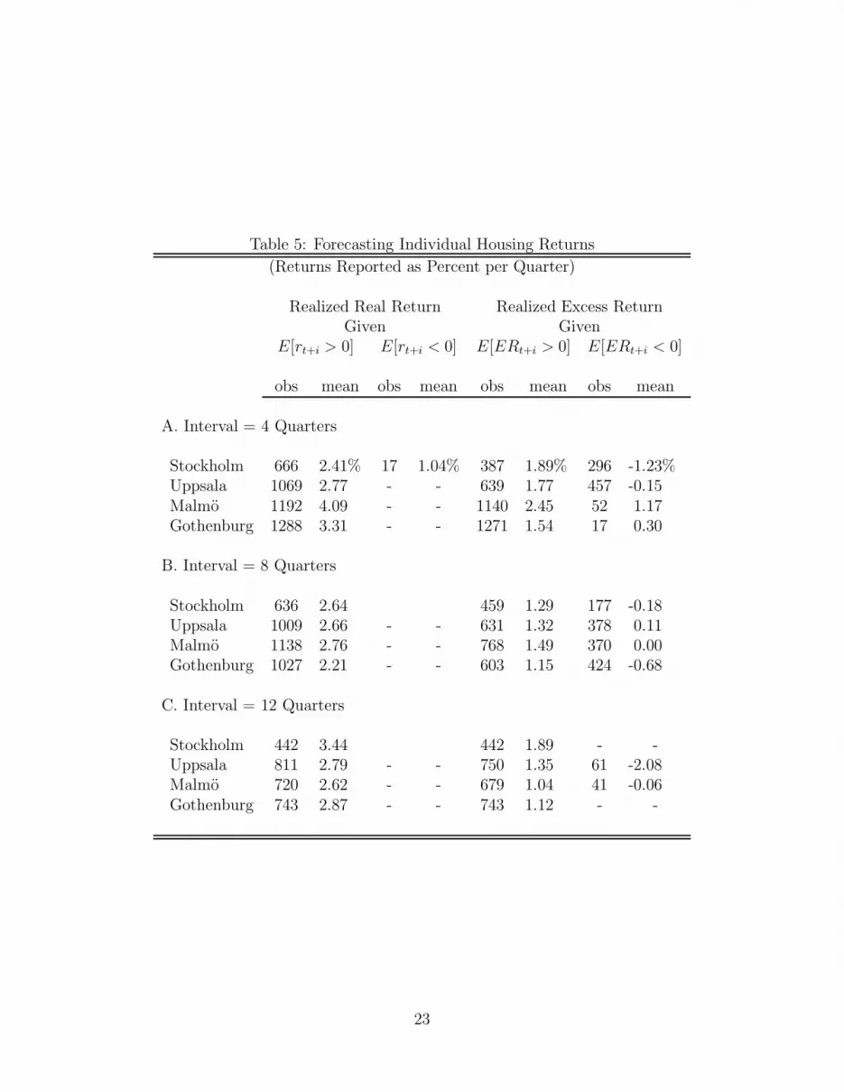
Table 5: Forecasting Individual Housing Returns

(Returns Reported as Percent per Quarter)

Realized Real Return Realized Excess ReturnGiven Given

E[rt+i > 0] E[rt+i < 0] E[ERt+i > 0] E[ERt+i < 0]

obs mean obs mean obs mean obs mean

A. Interval = 4 Quarters

Stockholm 666 2.41% 17 1.04% 387 1.89% 296 -1.23%Uppsala 1069 2.77 - - 639 1.77 457 -0.15Malmo 1192 4.09 - - 1140 2.45 52 1.17Gothenburg 1288 3.31 - - 1271 1.54 17 0.30

B. Interval = 8 Quarters

Stockholm 636 2.64 459 1.29 177 -0.18Uppsala 1009 2.66 - - 631 1.32 378 0.11Malmo 1138 2.76 - - 768 1.49 370 0.00Gothenburg 1027 2.21 - - 603 1.15 424 -0.68

C. Interval = 12 Quarters

Stockholm 442 3.44 442 1.89 - -Uppsala 811 2.79 - - 750 1.35 61 -2.08Malmo 720 2.62 - - 679 1.04 41 -0.06Gothenburg 743 2.87 - - 743 1.12 - -

23

Table 6: Transactions Costs

Costs reported as percent of house price, unless otherwise indicatedType of Buyer

MarketCost Timer Mover Speculator Investor

Registration,Inspection, none 2% 2% 2%Assessment

Tax on none none none 40% (of rent)Rental Income

Broker’s Fee none 5% 5% 5%at Sale

Capital Gains Tax none none 30% (of gain) 30% (of gain)

Clearly, these are simplifications, but the four buyers described above provide enough

detail to understand the approximate magnitude of the restraints on competition in housing

markets. For example, the tax on rental income is faced by owners who do not occupy their

dwelling. This institutional feature of housing markets penalizes the “investor” relative to

the other buyers, and represents a substantial barrier to entry for economic agents who are

strong forces for efficiency in other markets.

Based on the investment rule employed above (“purchase” if expected returns are positive,

realized profits from trade are calculated and presented in Tables 7 and 8. Table 7 shows

that, even after incorporating the appropriate costs, the real returns to housing are generally

positive for all four types of buyer. The increasingly higher costs facing the mover, the

speculator, and the investor, significantly reduce the realized real returns for each. In the

shortest interval, the investor experiences negative real returns, but as the interval increases

real returns rise, reflecting the amortization of the fixed costs incurred at purchase and sale.

Table 8 shows the realized excess returns for the same four types of buyers. The table

24

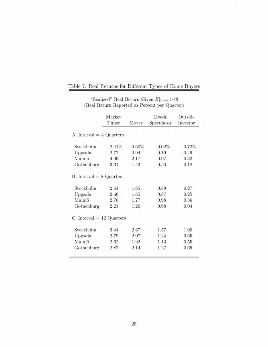
Table 7: Real Returns for Different Types of Home Buyers

“Realized” Real Return Given E[rt+i > 0](Real Return Reported as Percent per Quarter)

Market Live-in OutsideTimer Mover Speculator Investor

A. Interval = 4 Quarters

Stockholm 2.41% 0.60% -0.02% -0.72%Uppsala 2.77 0.94 0.19 -0.49Malmo 4.09 2.17 0.97 0.32Gothenburg 3.31 1.43 0.50 -0.18

B. Interval = 8 Quarters

Stockholm 2.64 1.65 0.89 0.27Uppsala 2.66 1.65 0.87 0.25Malmo 2.76 1.77 0.98 0.36Gothenburg 2.21 1.26 0.68 0.04

C. Interval = 12 Quarters

Stockholm 3.44 2.67 1.57 1.00Uppsala 2.79 2.07 1.24 0.65Malmo 2.62 1.92 1.13 0.55Gothenburg 2.87 2.14 1.27 0.69

25

Table 8: Excess Returns for Different Types of Home Buyers

“Realized” Excess Return Given E[rt+i > 0](Excess Return Reported as Percent per Quarter)

Market Live-in OutsideTimer Mover Speculator Investor

A. Interval = 4 Quarters

Stockholm 1.89% 0.01% -0.99% -1.68%Uppsala 1.77 -0.11 -1.11 -1.72Malmo 2.46 0.54 -0.67 -1.32Gothenburg 1.54 -0.34 -1.27 -1.95

B. Interval = 8 Quarters

Stockholm 1.29 0.29 -0.57 -1.18Uppsala 1.32 0.30 -0.59 -1.18Malmo 1.50 0.48 -0.46 -1.05Gothenburg 1.15 0.15 -0.65 -1.26

C. Interval = 12 Quarters

Stockholm 1.84 1.07 -0.03 -0.59Uppsala 1.35 0.62 -0.27 -0.86Malmo 1.04 0.33 -0.48 -1.06Gothenburg 1.20 0.47 -0.39 -0.98

differs sharply from the realized real returns in Table 7. After accounting for the costs

associated with investment in housing, excess returns are not as large as real returns. The

table shows that both the speculator and the investor lose money when buying and selling

housing over these three time horizons. The market timer, as in Case and Shiller (1989), is

able to make consistent excess returns by waiting for a positive forecast.

The most interesting result given in Table 8 is the returns experienced by the “mover.”

This type of buyer is the most common; the majority of housing transactions are not first time

purchases, but reflect adjustments to housing consumption. Most of these transactions do

not trigger capital gains taxes because the gains are reinvested in more expensive housing.

26

For these individuals, the excess returns are close to zero over the shortest interval, and

increase slightly as the interval increases. While this appears to be evidence that excess

returns are available to typical market participants, it should be noted that the costs of

moving have not been included because no data were available. It seems likely that the true

excess returns will be close to zero.

These results should hearten believers in competitive markets. Housing markets are

inefficient but do not offer arbitrage opportunities. For the majority of the participants

housing markets, the predictability of excess returns cannot be exploited. Furthermore, it

appears that market forces have driven the returns to housing to exactly the home owner’s

cost of capital after accounting for the fixed cost associated with buying and selling housing.

6 Conclusion

Past research on housing market efficiency has focused on the behavior of aggregate housing

prices. The general consensus from the literature is that aggregate housing prices and average

returns are predictable, which is a violation of market efficiency. However, it is typically

argued that the high costs associated with housing transactions prevents market forces from

competing away what appear to be excess profits.

The model presented in this paper addresses the question of housing market efficiency at

the level of the individual dwelling. By incorporating an appropriate error structure, which

reflect the prominent features of housing markets, into a general model of housing prices,

individual dwelling prices are shown quite clearly to follow a mean reverting process. This

result indicates that, at this level, housing markets are inefficient.

Case and Shiller’s (1989) speculation that “the house-specific component of the change in

log price is probably not homoskedastic but that the variance of the noise increases with the

interval between sales,” is correct. The results of this paper indicate that the error variance

is positively correlated with the interval of time between sales. However, the results also

indicate the the correlation is not one. Rather than following a random walk, the errors

are characterized more accurately as an autocorrelated process with a quarterly correlation

27

coefficient of about 0.9–pricing errors will persist for many years.

These results have implications for aggregate prices, but unfortunately do not offer an

opportunity for great wealth. The paper demonstrates that the serial correlation that char-

acterizes individual home prices is found also in aggregate prices. The results indicate that

for market timers–those for whom entry costs are sunk and capital gains taxes are mostly

irrelevant–there exists at least one strategy that earns excess returns. However, the in-

stitutional features of housing markets for owner-occupied housing prevent investors from

exploiting the apparent inefficiency to earn consistent excess profits. Indeed, it appears that

excess returns are predictable, but that they have been driven down to approximately the

fixed costs of buying and selling housing.

28

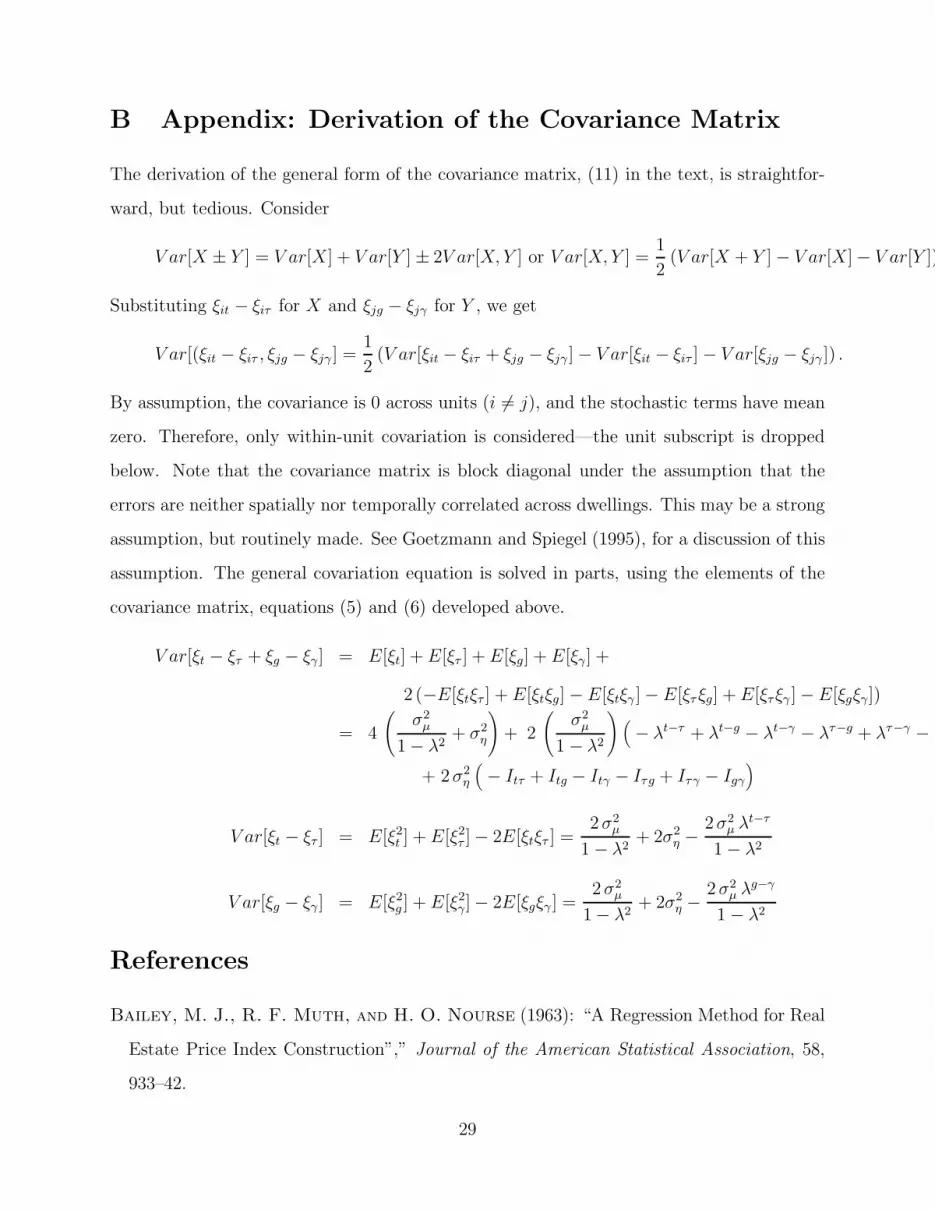
B Appendix: Derivation of the Covariance Matrix

The derivation of the general form of the covariance matrix, (11) in the text, is straightfor-

ward, but tedious. Consider

V ar[X ± Y ] = V ar[X] + V ar[Y ] ± 2V ar[X, Y ] or V ar[X, Y ] =1

2(V ar[X + Y ] − V ar[X] − V ar[Y ])

Substituting ξit − ξiτ for X and ξjg − ξjγ for Y , we get

V ar[(ξit − ξiτ , ξjg − ξjγ ] =1

2(V ar[ξit − ξiτ + ξjg − ξjγ ] − V ar[ξit − ξiτ ] − V ar[ξjg − ξjγ ]) .

By assumption, the covariance is 0 across units (i 6= j), and the stochastic terms have mean

zero. Therefore, only within-unit covariation is considered—the unit subscript is dropped

below. Note that the covariance matrix is block diagonal under the assumption that the

errors are neither spatially nor temporally correlated across dwellings. This may be a strong

assumption, but routinely made. See Goetzmann and Spiegel (1995), for a discussion of this

assumption. The general covariation equation is solved in parts, using the elements of the

covariance matrix, equations (5) and (6) developed above.

V ar[ξt − ξτ + ξg − ξγ] = E[ξt] + E[ξτ ] + E[ξg] + E[ξγ] +

2 (−E[ξtξτ ] + E[ξtξg] − E[ξtξγ ] − E[ξτξg] + E[ξτξγ ] − E[ξgξγ])

= 4

(σ2

µ

1 − λ2+ σ2

η

)+ 2

(σ2

µ

1 − λ2

)(− λt−τ + λt−g − λt−γ − λτ−g + λτ−γ − λ

+ 2σ2η

(− Itτ + Itg − Itγ − Iτg + Iτγ − Igγ

)

V ar[ξt − ξτ ] = E[ξ2t ] + E[ξ2

τ ] − 2E[ξtξτ ] =2σ2

µ

1 − λ2+ 2σ2

η −2σ2

µ λt−τ

1 − λ2

V ar[ξg − ξγ] = E[ξ2g ] + E[ξ2

γ] − 2E[ξgξγ ] =2σ2

µ

1 − λ2+ 2σ2

η −2σ2

µ λg−γ

1 − λ2

References

Bailey, M. J., R. F. Muth, and H. O. Nourse (1963): “A Regression Method for Real

Estate Price Index Construction”,” Journal of the American Statistical Association, 58,

933–42.

29

Case, K. E., and R. J. Shiller (1987): “Prices of Single-Family Homes since 1970: New

Indexes for Four Cities,” New England Economic Review, 0(0), 45–56.

(1989): “The Efficiency of the Market for Single-Family Homes,” American Eco-

nomic Review, 79(1), 125–37.

(1990): “Forecasting Prices and Excess Returns in the Housing Market,” American

Real Estate and Urban Economics Association Journal, 18(3), 253–73.

Englund, P., J. M. Quigley, and C. L. Redfearn (1998): “Improved Price Indexes

for Real Estate: Measuring the Course of Swedish Housing Prices,” Journal of Urban

Economics, 44(2), 171–96.

(1999a): “Do Housing Transactions Provide Misleading Evidence About the Course

of Housing Values?,” unpublished manuscript, pp. 1–26.

(1999b): “The Choice of Methodology for Computing Price Indexes: Comparisons

of Temporal Aggregation and Sample Definition,” Journal of Real Estate Finance and

Economics, 19(3), 91–112.

Gatzlaff, D. H. (1994): “Excess Returns, Inflation, and the Efficiency of the Housing

Market,” Journal of the American Real Estate and Urban EconomicsAssociation, 22(4),

553–81.

Gatzlaff, D. H., and D. R. Haurin (1997): “Sample Selection Bias and Repeat-Sales

Index Estimates,” Journal of Real Estate Finance and Economics, 14(1-2), 33–50.

(1998): “Sample Selection and Biases in Local House Value Indices,” Journal of

Urban Economics, 43(2), 199–222.

Goetzmann, W. N., and M. Spiegel (1995): “Non-temporal Components of Residential

Real Estate Appreciation,” Review of Economics and Statistics, 77(1), 199–206.

Grossman, S. J., and J. E. Stiglitz (1980): “On the Impossibility of Informationally

Efficient Markets,” American Economic Review, 70(3), 393–408.

30

Guntermann, K. L., and S. C. Norrbin (1991): “Empirical Tests of Real Estate Market

Efficiency,” Journal of Real Estate Finance and Economics, 4(3), 297–313.

Malpezzi, S. (1999): “A Simple Error Correction Model of Housing Prices,” Journal of

Housing Economics, 8(1), 27–62.

Quan, D. C., and J. M. Quigley (1991): “Price Formation and the Appraisal Function

in Real Estate Markets,” Journal of Real Estate Finance and Economics, 4(2), 127–46.

Soderberg, B. (1995): “Transaction Costs in the Market for Residential Real Estate,” De-

partment of Real Estate Economics Working Paper no. 20, Royal Institute of Technology,

Sweden, 20, 1–12.

31