introduction to value-at-risk (var
TRANSCRIPT

| ACE |
NTU – RISK MANAGEMENT SOCIETY – RESEARCH DEPARTMENT Page 1 of 10
Date of Presentation: 21 February 2013
Introduction to Value-at-Risk (VaR)
Executive Summary
Introduction and history of VaR
Three commonly used methods of quantifying VaR
Benefits and limitations
Case study on Citigroup
Contributors:
Ow-Yang Zhi Yan [email protected]
Zhou Xinzi [email protected]
Chia Zhiwei Isaiah [email protected]
Christoffer Alejandro Neil Ng
Meng Hui [email protected]
1.0 Introduction
For many that have invested or are considering investing in risky assets, it is often common to be
concerned about the maximum amount an investor can possibly lose on a particular investment
decision. Value at Risk (VaR) aims to provide a reasonable bounds answer. Due to the widespread
use of VaR as a tool for risk assessment, especially in financial service firms, this report aims to
briefly introduce to the reader the background, basic methods, benefits and limitations of the VaR
tool. A case study on Citigroup will also be examined.
By basic definition, VaR measures the potential loss in value of an asset over a defined period for a
given confidence interval. Any meaningful description of Value at Risk should comprise of three
components:
1. Time period,
2. Confidence level, and
3. VaR Amount (Loss Amount)
Hence, a typical VaR statement might look like this: “VaR on [Asset] is $100 million within a one-
week interval, 95% confidence level”
While VaR can be used by any entity to measure its risk exposure, it is widely used by commercial
banks, investment banks and most financial institutions to capture the potential loss in value of their
assets or portfolios from adverse market conditions over a specific period of time. This potential loss
| ACE |
NTU – RISK MANAGEMENT SOCIETY – RESEARCH DEPARTMENT Page 2 of 10
will then be compared against their available capital and cash reserves to ensure balance sheet
solvency.
VaR tries to capture the downside risk and potential losses. It is used by financial firms to prevent an
insolvency crisis, where a low-probability catastrophic occurrence creates a loss that wipes out the
firm’s entire capital base. It is to note that VaR can be defined more broadly or narrowly in specific
contexts, measuring risks in the form of interest rate changes, equity market volatility, and economic
growth.
1.1 History and Development of VaR
The impetus for the use of VaR measures came from the crisis that beset financial firms over time
and the regulatory responses to this crisis. In the aftermath of the Great Depression, Securities
Exchange Commission (SEC) required banks to keep borrowings below a specific equity capital. In the
decades thereafter, banks have consistently devised risk measures and control devices to ensure
that they meet these capital requirements.
With increased risk associated to derivatives markets and floating exchange rates in the early 1970s,
capital requirements were further refined. In 1980, SEC tied the capital requirements of financial
firms to the losses that would incur with 95% confidence over a thirty-day interval in different
security classes. In additional to stricter regulatory reporting demand, trading portfolios of
investment banks and commercial banks were becoming larger and more volatile. A more
sophisticated and timely set of risk control measures were thus needed.
By 1990s, many financial firms had already developed rudimentary measures of Value at Risk, with
wide variations on how it was measured. However, it was only in the aftermath of numerous
disastrous losses associated with the use of leverage and derivatives between 1993 and 1995,
coupled with the failure of Barings, that firms were ready for a more comprehensive risk measures.
In 1995, J.P. Morgan provided public access to data on the variances and co-variances across various
security and asset classes it had used internally to manage risk. This allows software makers to
develop software, based on the matrices made public and available to measure risk. The measure
was readily received by the commercial and investment banking, while regulatory authorities
welcomed this intuitive appeal. In the last decade, VaR has being widely used by financial firms and
is finding acceptance in non-financial firms.
2.0 Methodology
Next, we discuss the three popular computational methods used in calculating Value-at-Risk:
2.1 Historical Simulation (Empirical Distribution Function)
In the historical simulation method, we plot the empirical distribution of the metric (eg asset price,
asset return) that we are interested in, according to historical data. In other words, we do not
assume any theoretical distribution in this method and are therefore not interested in the mean,
standard deviation or any distribution parameter of the historical data. Instead we are only

| ACE |
NTU – RISK MANAGEMENT SOCIETY – RESEARCH DEPARTMENT Page 3 of 10
concerned about the actual frequencies of different occurrences in the historical distribution (within
a defined period).
After plotting the empirical distribution, we assume that history will repeat itself and that all
occurrences are independent and identically-distributed (iid). We then read off the results on the
left-tail of the curve to determine the worst outcome within our desired confidence level.
Figure 1: 1387 daily returns of stock QQQ. Source: ( Investopedia )
In the graph above, results of daily returns on the stock QQQ were collected on 1387 occasions and
plotted with the percentage return on the horizontal axis (worst returns on the left and best returns
on the right) against corresponding frequencies on the vertical axis. According to the graph, the
worst 5% of daily returns ranged from -4% to -8%. Therefore, in this situation, we can expect that
our daily return will exceed -4% with 95% confidence.
Other variations of the historical simulation method include the weighted historical simulation and
the filtered historical simulation.
2.2 Parametric (Variance-covariance) method
Under the parametric method, we make the strict assumption that our test subject follows a familiar
distribution, usually the Normal distribution. Based on historical data, we calculate the most likely
parameters (eg, mean and standard deviation) of the distribution and make necessary projections
with the use of these parameters.

| ACE |
NTU – RISK MANAGEMENT SOCIETY – RESEARCH DEPARTMENT Page 4 of 10
Figure 2: Fitting empirical results into a parametric distribution
As seen from the graph above, based on historical data (histogram), the likely mean and standard
deviation parameters are calculated, leading to the plotted theoretical normal distribution. The red
area represents the Value at Risk at 95% confidence.
The benefit of the parametric method over the historical simulation is that we know more properties
of the theoretical normal distribution than we know of the true distribution in historical simulation.
This grants us greater perceived knowledge of the risk distribution.
This method however, is not recommended for long horizons, portfolios with many options, or
assets with skewed distributions.
Example of Parametric calculation:
We express VaR = Market Price * Volatility [which is usually derived by: confidence
interval*standard deviation]
We have two assets within a portfolio, A and B
Price of A follows a normal distribution, with standard deviation 1%
Price of B follows a normal distribution, with standard deviation 1.5%
Correlation between A and B is 0.6
Calculate the VaR at 95% confidence interval:
Portfolio Value Volatility * 95% Confidence
Level Scaling Factor
VaR
A $1,000,000 1%*1.65 $16,500
B $1,000,000 1.5%*1.65 $24,750
| ACE |
NTU – RISK MANAGEMENT SOCIETY – RESEARCH DEPARTMENT Page 5 of 10
We use the formula:
= [16,5002 + 24,7502 + 2*0.6*24,750*16,500]1/2
= 37079.138 (being the Value at Risk of the portfolio at 95% confidence level)
Numerically, you might have also realized that the smaller the correlation between A and B, the
smaller the VaR for the portfolio of A and B as well.
2.3 Monte Carlo Simulation
The Monte Carlo method is the most complex and time-consuming of the three popular methods for
calculating VaR. In essence, the Monte Carlo simulation method involves the full re-pricing of an
asset based on algorithms that factor in current price, time, a number generated from a generator,
and other factors.
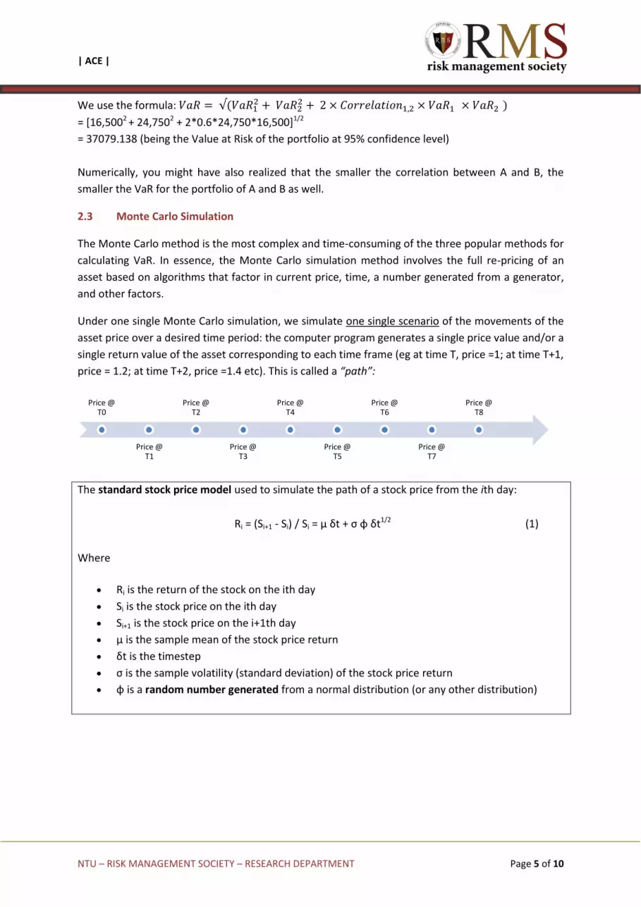
Under one single Monte Carlo simulation, we simulate one single scenario of the movements of the
asset price over a desired time period: the computer program generates a single price value and/or a
single return value of the asset corresponding to each time frame (eg at time T, price =1; at time T+1,
price = 1.2; at time T+2, price =1.4 etc). This is called a “path”:
The standard stock price model used to simulate the path of a stock price from the ith day:
Ri = (Si+1 - Si) / Si = μ δt + σ φ δt1/2 (1)
Where
Ri is the return of the stock on the ith day
Si is the stock price on the ith day
Si+1 is the stock price on the i+1th day
μ is the sample mean of the stock price return
δt is the timestep
σ is the sample volatility (standard deviation) of the stock price return
φ is a random number generated from a normal distribution (or any other distribution)
Price @ T0
Price @ T1
Price @ T2
Price @ T3
Price @ T4
Price @ T5
Price @ T6
Price @ T7
Price @ T8
| ACE |
NTU – RISK MANAGEMENT SOCIETY – RESEARCH DEPARTMENT Page 6 of 10
: : : : : : : : : : : : :
: : : : : : : : : : : : :
: : : : : : : : : : : : :
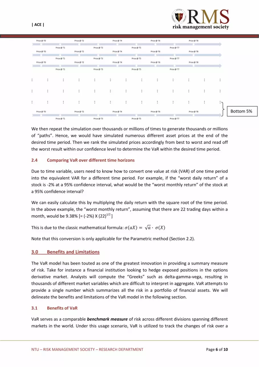
We then repeat the simulation over thousands or millions of times to generate thousands or millions
of “paths”. Hence, we would have simulated numerous different asset prices at the end of the
desired time period. Then we rank the simulated prices accordingly from best to worst and read off
the worst result within our confidence level to determine the VaR within the desired time period.
2.4 Comparing VaR over different time horizons
Due to time variable, users need to know how to convert one value at risk (VAR) of one time period
into the equivalent VAR for a different time period. For example, if the “worst daily return” of a
stock is -2% at a 95% confidence interval, what would be the “worst monthly return” of the stock at
a 95% confidence interval?
We can easily calculate this by multiplying the daily return with the square root of the time period.
In the above example, the “worst monthly return”, assuming that there are 22 trading days within a
month, would be 9.38% [= (-2%) X (22)1/2 ]
This is due to the classic mathematical formula:
Note that this conversion is only applicable for the Parametric method (Section 2.2).
3.0 Benefits and Limitations
The VaR model has been touted as one of the greatest innovation in providing a summary measure
of risk. Take for instance a financial institution looking to hedge exposed positions in the options
derivative market. Analysts will compute the “Greeks” such as delta-gamma-vega, resulting in
thousands of different market variables which are difficult to interpret in aggregate. VaR attempts to
provide a single number which summarizes all the risk in a portfolio of financial assets. We will
delineate the benefits and limitations of the VaR model in the following section.
3.1 Benefits of VaR
VaR serves as a comparable benchmark measure of risk across different divisions spanning different
markets in the world. Under this usage scenario, VaR is utilized to track the changes of risk over a
Price @ T0
Price @ T1
Price @ T2
Price @ T3
Price @ T4
Price @ T5
Price @ T6
Price @ T7
Price @ T8
Price @ T0
Price @ T1
Price @ T2
Price @ T3
Price @ T4
Price @ T5
Price @ T6
Price @ T7
Price @ T8
Price @ T0
Price @ T1
Price @ T2
Price @ T3
Price @ T4
Price @ T5
Price @ T6
Price @ T7
Price @ T8
Price @ T0
Price @ T1
Price @ T2
Price @ T3
Price @ T4
Price @ T5
Price @ T6
Price @ T7
Price @ T8 Bottom 5%
| ACE |
NTU – RISK MANAGEMENT SOCIETY – RESEARCH DEPARTMENT Page 7 of 10
time for use in a time-series analysis. In addition, a cross-sectional analysis can be performed by
comparing the different divisions in a certain time period to ensure compliance with the pre-
determined risk tolerance of the institution.
The VaR measure could be employed to maintain an equity cushion for a firm, effectively serving as
a measure of equity capital for a financial institution. A financial institution will determine an
adequate risk buffer based upon its risk aversion, and consequentially adjust the input of the
confidence level into the VaR model. This will allow the institution to not only ensure regulatory
compliance, but also effectively control its leverage adequately to avoid bankruptcy should the
market move in an unfavorable direction.
3.2 Limitations of VaR
As often as VaR is employed as first line of defense against market risk, practitioners should be
reminded of one of its limitations: the model does not provide an absolute loss estimate. As
discussed in the previous sections, the VaR benchmark provides a loss estimate at a pre-determined
level of confidence, and does not account for black swan events nor for increased kurtosis during a
crisis, which will increase the maximum absolute losses the institution could potentially incur.
VaR inherently assumes that the market exposure of the firm is fixed over a specified time horizon,
thus failing to account for differing risk exposure over the period. Volatility and the VaR measure
are often scaled by the square-root-of-time variable method to obtain a measure for the time
horizon of interest. The scaling factor does not account for change in exposure an institution would
have taken in response to changing market conditions.
Historical volatility data are used as inputs into the VaR model, which inherently assumes that
historical data proves to be a good predictor of the future. As such, stability risk exists because
historical data fails to account for structural surprises such as new regulatory requirements and
increase in correlation coefficients across financial assets during a crisis. The failure to incorporate
new information to predict future volatility will provide a grave underestimation of the risk.
Where historical data is not available as an input for the model, information risk does exist. For
instance, in situations such as the pricing of risk for an initial public offering, in a private placement,
or derivatives traded in the over-the-counter market, proxies are used in these scenarios, and the
reliability and accuracy of the estimate is highly dependent on the supposed correlation between
the proxy of choice and the financial instrument of interest.
4. 0 Case Study
Having learnt the various aspects of value at risk, let us now look at how VaR played a role in the
2008 financial crisis.
In 2008, a typical investment portfolio of 60% stocks and 40% bonds lost about 20% of its value.
Standard portfolio-construction tools assume that such an event will only happen once every 111
years. Using a fat-tailed distribution, however, such an occurrence was predicted to possibly happen
once every 40 years. This number obtained might be due to the fact that number crunchers who
have a smaller supply of historical observations to construct models tended to focus on rare events.
| ACE |
NTU – RISK MANAGEMENT SOCIETY – RESEARCH DEPARTMENT Page 8 of 10
The “Value-at-Risk” model is widely used due to the ease of understanding compared to the other
available risk measures. In fact, it is so easy to understand that some bank managers may have went
one step further from using VaR as a risk measure to relying on it for risk management.
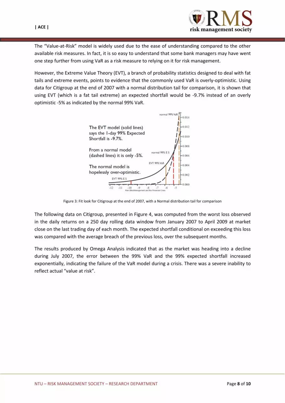
However, the Extreme Value Theory (EVT), a branch of probability statistics designed to deal with fat
tails and extreme events, points to evidence that the commonly used VaR is overly-optimistic. Using
data for Citigroup at the end of 2007 with a normal distribution tail for comparison, it is shown that
using EVT (which is a fat tail extreme) an expected shortfall would be -9.7% instead of an overly
optimistic -5% as indicated by the normal 99% VaR.
Figure 3: Fit look for Citigroup at the end of 2007, with a Normal distribution tail for comparison
The following data on Citigroup, presented in Figure 4, was computed from the worst loss observed
in the daily returns on a 250 day rolling data window from January 2007 to April 2009 at market
close on the last trading day of each month. The expected shortfall conditional on exceeding this loss
was compared with the average breach of the previous loss, over the subsequent months.
The results produced by Omega Analysis indicated that as the market was heading into a decline
during July 2007, the error between the 99% VaR and the 99% expected shortfall increased
exponentially, indicating the failure of the VaR model during a crisis. There was a severe inability to
reflect actual “value at risk”.

| ACE |
NTU – RISK MANAGEMENT SOCIETY – RESEARCH DEPARTMENT Page 9 of 10
Figure 4: Estimate EVT-based 99% VaR and 99% Expected Shortfall daily from January 2004 to June 2009
–A risk-controlled portfolio of Citigroup shares and cash, with a target 1-day 99% Expected Shortfall of -4% (No short positions)
Many managers who heavily relied on the VaR model had heavily leveraged their portfolios.
Depending on the degree of leverage, losses could be painfully magnified. The interaction of
extreme leverage and the rapidly falling value of whatever was held in the portfolio led to the wipe-
out of vulnerable firms, and eventually mergers, bailouts, and loss of confidence in the financial
system. The implication is that the misuse of a risk measure, VaR, led to a degree of unwarranted
comfort with the leveraged position of the firm.
The findings from this case were not specific to Citigroup or the Dow Jones Index alone; similar
analysis revealed very similar situations for other entities such as Lehman Brothers, Halifax Bank of
Scotland, Royal Bank of Scotland, BNP Paribas, ING. Equity indices worldwide and other asset classes
such as hedge fund indices also showed similar characteristics. The use of other EVT methods also
produced similar results.
As many investors were clobbered by the financial crisis and many investment firms lost significant
portions of their assets under management, enhanced risk management has become a current
priority for most in the industry. VaR, however, will continue to be used as a way to communicate
risk.
5.0 Conclusion
VaR is not necessarily less effective than other risk measures used, since standard deviation is one of
the most commonly used risk measures in the industry. VaR improves on standard deviation in that
standard deviation is not an intuitive concept to most investors. VaR is stated in terms of the dollar
value of the portfolio, so it is a more intuitive estimate of risk. However, exclusive reliance on VaR
without due consideration of the tail risk of extreme losses had clearly led to painful losses. The
lessons we should take away from the financial crisis include the need to watch out for over-reliance
on VaR or any one tool alone. We need to prepare for downside events beyond the “expected
downside” quantified by VaR, even if these events are of a small probability. A proper understanding
of VaR should lead to productive discussions of the risk of extreme losses, the investor’s appetite for
such risk, and strategies for managing the risk-return trade-offs.

| ACE |
NTU – RISK MANAGEMENT SOCIETY – RESEARCH DEPARTMENT Page 10 of 10
References
Berry Romain(n.d.). An Overview of Value-at-Risk: Part III – Monte Carlo Simulations VaR J.P. Morgan Investment Analytics
&Consulting, extracted from:
http://www.jpmorgan.com/tss/General/Risk_Management/1159380637650
Chen, W., Skoglund, J., & Erdman, D. (Spring 2010). The performance of value-at-risk models during the crisis. The Journal
of Risk Model Validation.
Investopedia (n.d). An Introduction To Value at Risk (VAR), extracted from:
http://www.investopedia.com/articles/04/092904.asp#axzz2Ka4jT4Ng
Kourouma, L., Dupre, D., Sanfilippo, G., & Taramasco, O. (2012). Extreme Value at Risk and Expected Shortfall during
Financial Crisis. France: Doctoral School of Management.
Nicklas Norling, D. S. (n.d.). An empirical evaluation of Value-at-Risk during the financial crisis. Sweden: Lund University,
School of Economics Management,Department of Business Administration.
Pohlmeier, R. C. (2009). How Risky is the Value-at-Risk ? Evidence from Financial Crisis. Rimini: Rimini Center for Economic
Analysis.
RiskMetrics Group (n.d.). VaR: Parametric Method, Monte Carlo Simulation, Historical Simulation, extracted from:
http://help.riskmetrics.com/RiskManager3/Content/Statistics_Reference/VaR.htm
Saša Žiković, B. A. (2009). Global fi nancial crisis and VaR performance in emerging markets: A case of EU candidate states -
Turkey and Croatia. Zb. rad. Ekon. fak. Rij, 149-170.
Saunders, A., & Allen, L. (2002). New Approaches to Value at Risk and Other Paradigms. New York: John Wiley & Sons, Inc.
Shadwick, D. W. (2010, Febuary 25). Risk (Mis) Management and the Financial Crisis The Impact of the All Too Probable.
Omega Analysis. Hawaii, United States of America: University of Hawaii Mathematics Department.
Disclaimer
The information set forth herein has been obtained or derived from sources generally available to the public and believed
by the author(s) to be reliable, but the author(s) does not make any representation or warranty, express or implied, as to
its accuracy or completeness. The information is not intended to be used as the basis of any investment decisions by any
person or entity. This information does not constitute investment advice, nor is it an offer or a solicitation of an offer to
buy or sell any security. This report should not be considered to be a recommendation by any individual affiliated with NTU
RMS Research Department.