Centre forComputationalFinance andEconomicAgents

WorkingPaperSeries

www.ccfea.net

WP013-07

Amadeo AlentornSheri Markose

Generalized Extreme ValueDistribution and Extreme

Economic Value at Risk(EE-VaR)

October 2007

Generalized Extreme Value Distribution andExtreme Economic Value at Risk (EE-VaR)

Amadeo Alentorn∗and Sheri Markose†

September, 2007

Abstract

Ait-Sahalia and Lo (2000) and Panigirtzoglou and Skiadopoulos (2004)have argued that Economic VaR (E-VaR), calculated under the optionmarket implied risk neutral density is a more relevant measure of riskthan historically based VaR. As industry practice requires VaR at highconfidence level of 99%, we propose Extreme Economic Value at Risk(EE-VaR) as a new risk measure, based on the Generalized Extreme Value(GEV) distribution. Markose and Alentorn (2005) have developed a GEVoption pricing model and shown that the GEV implied RND can accu-rately capture negative skewness and fat tails, with the latter explicitlydetermined by the market implied tail index. Here, we estimate the termstructure of the GEV based RNDs, which allows us to calibrate an em-pirical scaling law for EE-VaR, and thus, obtain daily EE-VaR for anytime horizon. Backtesting results for the FTSE 100 index from 1997 to2003, show that EE-VaR has fewer violations than historical VaR. Fur-ther, there are substantial savings in risk capital with EE-VaR at 99%as compared to historical VaR corrected by a factor of 3 to satisfy theviolation bound. The efficiency of EE-VaR arises because an implied VaRestimate responds quickly to market events and in some cases even antici-pates them. In contrast, historical VaR reflects extreme losses in the pastfor longer.

∗Centre for Computational Finance and Economic Agents (CCFEA), Old Mutual AssetManagers (UK) Ltd

†Centre for Computational Finance and Economic Agents (CCFEA),Department of Eco-nomics, University of Essex. Corresponding author: Sheri Markose. Email address:scher@essex.ac.uk We are grateful for comments from two anonymous referees which haveimproved the paper. We acknowledge useful discussions with Thomas Lux, Olaf Menkens,Christian Schlag, Christoph Schleicher, Radu Tunaru and participants at the FMA 2005 atSiena and CEF 2005 in Washington DC.

1

JEL classification: G10, G14.Keywords: Economic Value-at-Risk, EE-VaR, empirical scaling law,

term structure of implied RNDs.

1 Introduction

Value-at-Risk (VaR) has become the most popular measure for risk man-agement. Value-at- Risk, denoted by VaR (q, k), is an estimate, for a givenconfidence level q, of the maximum that can be lost from a portfolio over a giventime horizon k. An alternative measure of risk is the Economic VaR (E-VaR)proposed by Ait-Sahalia and Lo (2000) and calculated under the option-impliedrisk neutral density. It has been argued that E-VaR is a more general measure ofrisk, since it incorporates investor risk preferences, demand–supply effects, andmarket implied probabilities of losses or gains, Panigirtzoglou and Skiadopoulos(2004). E-VaR can be seen as a forward looking measure to quantify marketsentiment about the future course of financial asset prices, whereas historicalor statistically based VaR (S-VaR) is backward looking, based on the historicaldata. With the development in 1993 of the traded option implied VIX indexfor the SP-500 returns volatility over a 30 calendar day horizon, the so called“investor fear gauge”, a significant move toward the use of a market impliedrather than a historical measure of risk in practical aspects of risk managementhas occurred. Policy makers such as the Bank of England use traded optionimplied risk neutral density, volatility and quantile measures to gauge marketsentiment regarding future asset prices. 1

Given the industry standard for 10 day VaR at high confidence levels of 99%,it is important to correctly model the distribution of the extreme values of assetreturns, as it is well known that the probability distributions of asset returns arenot Gaussian especially at short time horizons (see, Cont, 2001). In the man-agement of risk, the modelling of asymmetries and the asymptotic behaviour ofthe tails of the distribution of losses is important. Extreme value theory is arobust framework to analyse the tail behaviour of distributions. Extreme valuetheory has been applied extensively in hydrology, climatology and also in the

1For the VIX index see www.cboe.com/micro/vix/ and for the Bank of England op-tion traded implied probability density functions, volatility and quantile measures see,www.bankofengland.co.uk/statistics/impliedpdfs/ . In particular, market risk premia for agiven holding period is estimated as payoffs from volatility swaps which effectively take thedifference between realized volatility and the option implied volatility.

2

insurance industry (see, Embrechts et. al. 1997). Despite early work by Man-delbrot (1963) on the possibility of fat tails in financial data and evidence on theinapplicability of the assumption of log normality in option pricing, a system-atic study of extreme value theory for financial modelling and risk managementhas only begun recently. Embrechts et. al. (1997) is a comprehensive sourceon extreme value theory and applications.2 Dacorogna et. al. (2001) developa VaR estimate based on the extreme value Pareto distribution for the tails ofthe distribution which is then empirically estimated from high frequency datausing a bootstrap method for the Hill estimator.

In this paper we propose Extreme Economic Value at Risk (EE-VaR) as anew risk measure, which is calculated from an implied risk neutral density thatis based on the Generalized Extreme Value (GEV) distribution. It has beenshown in Markose and Alentorn (2005) that the GEV option pricing modelnot only accurately captures the negative skewness and higher kurtosis of theimplied risk neutral density (RND), but it also delivers the market implied tailindex that governs the tail shape. It is important to note that the GEV does notpose a priori restrictions on the tail shape as the GEV distribution encompassesthe thin and short tailed class of the Gumbel and Weibull , respectively, alongwith the fat tailed Fréchet.3 Indeed, one of the main findings from Alentorn andMarkose (2006) and Alentorn (2007) is that the daily implied tail shape parame-ter estimated without maturity effects from the GEV RND model indicates thatmarket perception of fat tailed behaviour of extreme events is interspersed withthin and short tailed Gumbel and Weibull values.4 Hence, the assumption of theGEV parametric model for the RND overcomes problems, associated with theestimation of the risk neutral density function to flexibly include extreme valuesand fat tails, which are often encountered with many non-parametric methodsand with the use of parametric models such as the Gaussian.5 In this paper we

2Embrechts (1999, 2000) considers the potential and limitations of extreme value theory forrisk management. Without being exhaustive here, De Haan et. al. (1994) and Danielsson andde Vries (1997) study quantile estimation. Bali (2003) uses the GEV distribution to modelthe empirical distribution of returns. Mc Neil (1999) gives an extensive overview of extremevalue theory for risk management. See also Dowd (2002, pp.272-284).

3The Gumbel class includes the normal, exponential, gamma and log normal while theWeibull include distributions such as the uniform and beta. Examples of fat tailed distribu-tions that belong to the Fréchet class are Pareto, Cauchy, Student-t and mixture distributions.

4Even during extreme events, though the implied tail index results in fat tails for the GEVRND based returns– at all times the first four moments were bounded.

5In order to estimate risks at high confidence levels, such as 99% - many non-parametricmethods for RND estimation fail to capture tail behaviour of distributions because of sparsedata for options traded at very high or very low strike prices. Hence, parametric models havebecome unavoidable. This, however, replaces sampling error by model error. Markose and

3

will focus on estimating the term structure of the GEV based implied RNDs,which allows us to calibrate an empirical scaling law for EE-VaR at differentconfidence levels, and thus, to obtain the daily EE-VaR for any time horizon,without having to employ the widely used but incorrect square root of timescaling rule.

There is a vast literature on the analysis of information implied from optionmarkets. One of the areas that has received the most attention is the study ofthe implied volatility surfaces, such as in Day and Craig (1988), Ncube (1996),Dumas, Fleming and Whalley (1998) and others. The great majority of studiesof implied distributions have focused on the analysis of the distributions at asingle point in time for event studies, such as Bates (1991) for the study of the1987 crash, Gemmill and Saflekos (2000) for the study of British elections, andMelick and Thomas (1996) for the analysis of oil prices during the Gulf warcrisis. Starting with the study of the day to day dynamics of implied volatilitysurfaces (see Cont and Da Fonseca (2002)), recently, Clews et. al. (2001) andPanigirtzoglou and Skiadopoulos (2004) have developed a framework for theanalysis of dynamics of implied RND functions.

A problem encountered when looking at the daily dynamics of RNDs, orRND implied measures such as volatility6 or their associated quantile values, theE-VaR, is the time to maturity and the contract switch effects (see, Melick andThomas, 1998). RNDs are usually constructed using the options with shortesttime to maturity. Since options have a fixed expiry date, this means that boththe time horizon of the RND and the holding period of the underlying assetchange with time to maturity. The degree of uncertainty decreases as the expirydate approaches. Uncertainty jumps up again when the option with the shortesttime to maturity expires, and we switch to options with the next expirationdate. For instance, given that options on the FTSE 100 index expire on thethird Friday of the expiry month, the jump would occur on the third Mondayof the expiry month. Note also that option prices with less than 5 working daysto maturity are usually excluded. Thus, the problem associated with obtainingconstant horizon RNDs and option implied values for VaR or volatility for theunderlying assets from traded options is non-trivial. Clearly, the use of E-VaR

Alentorn (2005) have argued that as the GEV distribution encompasses the 3 main classesof tail behaviour, it mitigates model error and further there is parsimony in the number ofparameters necessary to define the distribution.

6Alentorn and Markose (2006) give an extensive survey of the studies done on removingmaturity effects on implied volatility and higher moments of the RND. Here, we focus on thequantile values, E-VaR.

4

for risk management is feasible only if it can be calculated and reported dailyfor a constant time horizon or holding period that is required.

With regard to the traded option implied E-VaR, to our knowledge, thereare only three previous studies that have carried out an empirical analysis ofE-VaR and two of these study daily constant horizon E-VaR. Ait-Sahalia andLo (2000) estimated the E-VaR for a 126 day horizon. Clews et al. (2001)have suggested a semi-parametric methodology that can remove maturity effectsin the construction of constant horizon RNDs. The methodology consists ofinterpolating the Black-Scholes implied volatility surface in delta space at agiven time horizon, and then deriving the implied RND by calculating the secondderivative of the call pricing function, using the Breeden and Litzenberger (1978)result. This methodology is used by the Monetary Instruments and MarketsDivision at the Bank of England to report daily E-VaR values for the FTSE100 index at confidence levels ranging from 5% to 95% for the FTSE 100, fora 3 month constant horizon RND. However, with this methodology, it is notpossible to construct a constant time horizon implied RND for a time horizonshorter than the shortest maturity available, given that the implied volatilitysurface in delta space is non-linear. Panigirtzoglou and Skiadopoulos (2004)looked at the E-VaR calculated at 95% confidence level for constant horizons of1, 3 and 6 months for every 14 days during the year 2001. However, the problemof reporting daily E-VaR at short constant horizons such as 10 days remains andtypically semi-parametric methods for RND extraction fail to report E-VaR at99% confidence level.

In this paper, we focus on obtaining a daily estimate of a constant timehorizon GEV based E-VaR using a discrete term structure of RNDs. In Sec-tion 2, the new methodology we propose proceeds by first constructing a dailydiscrete term structure of implied RNDs, using option prices of all maturitiesavailable and a cross section of strikes for each maturity. Hence, there is aRND for each maturity available for traded options in a given day. Assumingthe parametric GEV model for the RND, we calculate the EE-VaR at differentconfidence levels as the quantile values for the RND for each available maturity.We exploit the linear behaviour of quantile values vis-à-vis the holding period,k, in the log-log scale to derive an empirical scaling law for different confidencelevels, q.7 One of the advantages of this linear relationship is that it allows us

7The empirical evidence for the scaling parameter b in the relationship, V aR(q, k) =V aR(q, 1)kb, which is linear in logs has been studied by Hauksson (2001), Menkens (2004)and Provizionatou et. al.(2005) in the context of historical VaR. Also, Dacorogna et. al.

5

to both interpolate and extrapolate from the available maturities and obtaindaily E-VaR values for any constant horizon from 1 day to m days and can beused regardless of the method for extracting the discrete RNDs. To test therobustness of our methodology we use the daily 90 day E-VaR reported by theBank of England for the 95% confidence level to compare the performance ofthe GEV implied EE-VaR and also E-VaRs obtained from parametric RNDsfor the Black Scholes and the Mixture of two Lognormals. We then proceedto report a 10 day EE-VaR which is easily done with our method regardlessof the time horizon of the closest maturity option contracts. We analyse theperformance of EE-VaR for different confidence levels, different time horizons,and for a large dataset, and compare it with the performance of historical VaRand the Black-Scholes E-VaR. In this paper we perform an in depth analysis ofthe daily EE-VaR performance for over 7 years, using daily closing index optionprices on the FTSE 100 from 1997 to 2003. This is the first paper to do thisand the empirical implementation and results are reported in Sections 3 and 4.Backtesting results, based on the FTSE 100 index from 1997 to 2003, show thatEE-VaR has fewer violations than historical VaR. Note that statistical VaR isdone for a 1 day return and then scaled by the square root of time rule. The 10day S-VaR when corrected by a multiplication factor of 3, to satisfy the viola-tion bound, requires substantially more risk capital than EE-VaR. This savingin risk capital with EE-VaR at high confidence levels of 99% arises because animplied VaR estimate responds quickly to market events and in some cases evenanticipate them. In contrast, VaR estimates based on historical data reflectextreme losses in the past for longer.

2 Model and Methodology

2.1 Extraction of GEV based RND from option prices

A large number of methods have been proposed for extracting implied distri-butions from option prices since the seminal work of Breeden and Litzenberger(1978), (see Jackwerth (1999) for an extensive survey). In this paper we use themethodology proposed by Markose and Alentorn (2005) based on the General-ized Extreme Value (GEV) distribution.

Let St denote the underlying asset price at time t. The European call option

(2001) derived an extreme value based VaR scaling law for high frequency forex data. Here,we investigate the scaling relationship for implied VaR, rather than for historical VaR.

6

Ct is written on this asset with strike K and maturity T . We assume theinterest rate r is constant. Following the Harrison and Pliska (1981) result onthe arbitrage free European call option price, there exists a risk neutral density(RND) function, g(ST ), such that the equilibrium call option price can bewrittenas:

Ct (K) = EQt [e−r(T−t)max (ST −K, 0)]

= e−r(T−t)

ˆ ∞K

(ST −K) g (ST ) dST . (1)

Also, the following martingale condition holds for the stock price

St = e−r(T−t)EQt [ST ]. (2)

Here EQt [.] is the risk-neutral expectation operator, conditional on all infor-

mation available at time t, and g(ST ) is the risk-neutral density function of theunderlying at maturity. Note that the GEV option pricing model in Markoseand Alentorn (2005) is based on the assumption that negative returns, LT , asdefined in equation (3) below, follow a GEV distribution:

LT = −RT = −ST − St

St= 1− ST

St. (3)

The GEV distribution, in the form in von Mises (1936) (see, Reiss andThomas, 2001, p. 16-17) which incorporates a location parameter µ, a scaleparameter σ, and a tail shape parameter ξ, is defined by:

Fξ,µ,σ(x) = exp

(−(

1 +ξ

σ(x− µ)

)−1/ξ)

, ξ 6= 0, (4)

with1 + ξ

(x− µ)σ

> 0,

andF0,µ,σ (x) = exp

(−exp

(x− µ

σ

)), ξ = 0. (5)

The tail shape parameter ξ = 0 yields thin tailed distributions with the socalled tail index 1/ξ = α being equal to infinity, implying that all momentsof this class of distributions exist. When ξ < 0 the GEV distribution class isWeibull. The fat tailed Fréchet distributions arise when ξ > 0 and note ξ > 25

7

is sufficient to imply infinite kurtosis.The RND function g(ST ) in (1) for the underlying asset price given that

LT is assumed to satisfy the GEV density function (see, Reiss and Thomas, p.16-17) is given by8:

g(ST ) =1

Stσ

(1 +

ξ (LT − µ)σ

)−1−1/ξ

exp

(−(

1 +ξ (LT − µ)

σ

)−1/ξ)

, (6)

with1 +

ξ

σ(LT − µ) = 1 +

ξ

σ

(1− ST

St− µ

)> 0. (7)

Note if the above condition in (7) is not satisfied, the GEV density function isnot defined on the real line. When ξ > 0 and the distribution for Lt is fat tailed,condition (7) implies that the GEV density function for the price is truncatedon the right, that is, the probability that the price will rise above this truncationvalue is zero. On the other hand, when the ξ < 0 and Lt is Weibull class, theGEV density function for ST is truncated on the left implying that the pricewill not fall below the truncation value. Markose and Alentorn (2005) find thatwhile this did affect the limits of integration for the option price equation in(1), the closed form solution for the call (and put) option for all cases of ξ 6= 0is identical. Omitting the proof , which can be found in Markose and Alentorn(2005) the closed form GEV RND based call option price is given by

Ct (K) = e−r(T−t){−Stσ

ξΓ(1− ξ, H−1/ξ)

−(St(1− µ +σ

ξ)−K)(−e−H−1/ξ

)}, (8)

where H = 1 + ξσ

(1− K

St− µ

)and Γ(1 − ξ,H−1/ξ) =

´∞H−1/ξ z−ξe−zdz is the

incomplete Gamma function.The structural GEV parameters ξ, µ and σ can be estimated by minimizing

the sum of squared errors (SSE) between the analytical solution of the GEVoption pricing equations in (8) and the observed traded option prices with strikesKi, as given in (9) below:

SSE(t) = minξ,µ,σ

{N∑

i=1

(Ct (Ki)− Ct((Ki)

)2}

. (9)

8Note the relationship between the density function for Lt, f(Lt) , and that for the under-lying, g(ST ), is given by the general formula g(ST ) = f(LT )| ∂LT

∂ST| = f(LT ) 1

St.

8

For purposes of comparison, we use the above method to back out the re-spective implied parameters for the Black-Scholes model and also the RND fromthe Mixture of two Lognormals (MLN) first constructed by Ritchey (1990).

At the estimation stage, we use the data on the index futures contract withthe same maturity as the options and as the futures price at maturity yields,FT = ST , the no arbitrage martingale condition in (2) enables us to substituteout EQ(ST ) by using Ft,T = EQ(ST ), This also vitiates the need for data on thedividend yield rate. The optimization problem in (10), was performed using thenon-linear least squares algorithm from the Optimization toolbox in MatLab.9

2.2 EE-VaR calculation from GEV RND

The quantile for the GEV distribution i.e. the VaR value associated witha given confidence level q, is given as a function of the three GEV parameters(see, Dowd 2004: pp. 274):

V aR = µ− σ

ξ

[1− (− log (q))−ξ

], ξ 6= 0, (10)

and

V aR = µ− σ log [log (1/q)] , ξ = 0. (11)

On substituting the implied GEV parameters from daily traded option pricesfor a given maturity horizon, the extreme economic value at risk (EE-VaR) iscalculated from (10) and (11).

The results obtained using EE-VaR will be compared with E-VaR valuesunder the Gaussian assumptions of the Black-Scholes model and that of themixture of two lognormals. The quantile of the normal distribution is usedto calculate the E-VaR values for the Gaussian case using the Black-Scholesimplied volatility. The MLN method models the RND as a weighted sum of twolognormals, and is given by:

f(ST ) = ph(ST | µ1T, σ1

√T ) + (1− p)h(ST | µ2, σ2

√T ). (12)

The MLN RND has been extensively used in the literature, given that it is9For a more detailed analysis of the estimation results, including time series of implied

parameters, pricing performance and comparison of results of the GEV model with otherparametric models, can be found in Alentorn and Markose (2006) and Alentorn (2007). Asalready noted in the Introduction, the daily implied tail shape parameters ξ, for the sampleperiod ranged between -0.2 and +0.22.

9

very flexible, and allows the modelling of different levels of skewness, as well asbimodal densities. However, compared to the GEV RND it has are five unknownparameters θ = {µ1, µ2, σ1, σ2, p}, the means of each lognormal function µ1andµ2 , the standard deviations σ1and σ2 , and the weighting coefficient p. Weobtain the set of implied parameters θ by the method in (9). Then, E-VaR iscalculated as the quantile of the MLN density, which consists of a weighted sumof the two inverse cumulative distribution functions, H , and given by:

E − V aR(q, k) = pH−1 (q | µ1, σ1, T ) + (1− p) H−1 (q | µ2, σ2, T ) . (13)

Some authors, such as Shiratsuka (2001) and Melick (1999), argue that thevalues for the higher quantiles of implied RNDs are very sensitive to the choiceof RND estimation technique, since the range of strike prices that are actuallytraded is very limited and the tails of the estimated implied RND vary dependingon the procedure employed. Table 1 below shows the percentage number of daysbetween 1997 and 2003 with traded put options with strike below each of theconfidence levels.

Table 1: Percentage number of days with put option prices with strikes beloweach of the confidence levels FTSE-100 Traded Options (1997-2003)Confidenc level Percentage number of days

70% 94%80% 86%90% 68%95% 51%99% 22%

Hence, we will also compare the quantile values obtained from the parametricRND models with those at the highest confidence level of 95% reported by theBank of England which uses the semi-parametric RND method discussed earlier.

3 Data description

The data used in this study are the daily settlement prices of the FTSE100 index call and put options published by the London International FinancialFutures and Options Exchange (LIFFE). These settlement prices are based onquotes and transactions during the day and are used to mark options and futurespositions to market. Options are listed at expiry dates for the nearest threemonths and for the nearest March, June, September and December. FTSE 100

10

options expire on the third Friday of the expiry month. The FTSE 100 optionstrikes are in intervals of 50 or 100 points depending on time-to-expiry, and theminimum tick size is 0.5.

The period of study was from 1997 to 2003, so there were 28 expirationdates (7 years with 4 contracts per year). This period includes some events,such as the Asian crisis, the LTCM crisis and the 9/11 attacks, which resultedin a sudden fall of the underlying FTSE 100 index, and will be useful to analyzethe performance of the methods under extreme events. The average number ofmaturities available with more than 3 options traded in our sample (1997-2003)is displayed in Table 2 below . In average across all years, we have 5.33 differentmaturities each day.

Table 2: Average number of maturities available FTSE-100 Traded Options(1997-2003)

Year Average number of maturities available1997 3.961998 4.571999 5.192000 5.492001 5.842002 6.192003 6.09

Average 5.33

The LIFFE exchange quotes settlement prices for a wide range of options,even though some of them may have not been traded on a given day. In thisstudy we only consider prices of traded options, that is, options that have a non-zero volume. The data were also filtered to exclude days when the cross-sectionsof options had less than three option strikes, since a minimum of three strikesis required to estimate the three parameters of the GEV model.10Also, optionswhose prices were quoted as zero or that had less than 5 days to expiry wereeliminated. Finally, option prices were checked for violations of the monotonicitycondition.11

10The number of option prices needed to extract the RND must be at least equal than thenumber of degrees of freedom for the parametric method used. The number of degrees offreedom is equal to the number of parameters that need to be estimated minus the numberof constraints. For example, the GEV model has three parameters while the mixture oflognormals have five parameters.

11Monotonicity requires that the call (put) prices are strictly decreasing (increasing) withrespect to the exercise price.

11

The risk-free rates used are the British Bankers Association’s 11 a.m. fixingsof the 3-month Short Sterling London InterBank Offer Rate (LIBOR) rates fromthe website www.bba.org.uk. Even though the 3-month LIBOR market does notprovide a maturity-matched interest rate, it has the advantages of liquidity andof approximating the actual market borrowing and lending rates faced by optionmarket participants (Bliss and Panigirtzoglou, 2004).

4 Empirical Modelling and Results

4.1 Term structure of RNDs

To calculate the EE-VaR, ideally, one would use a RND implied by optionswith time to maturity exactly equal to the time horizon we are interested. Thatis, to calculate the 10 day EE-VaR we would use prices from options that maturein 10 days to obtain an implied RND, and calculate the quantile of that densityat the confidence level required. However, in practice, we only have options thatexpire every month during the next three months, and also, options that expirein March, June, September and December. In the original study of Markoseand Alentorn (2005), at each trading day, only the RND implied by the closestto maturity contracts for which futures contracts were available (March, June,September and December) was extracted. Here, we propose, on a daily basis,the extraction of an RND for each of the maturities with a sufficient number oftraded option prices. Then, using this discrete set of RNDs, each with a differentmaturity, we can construct what we call a term structure of implied RNDs. Thisterm structure can be visualized as a 3 dimensional chart that displays, for agiven day, how the implied RNDs vary across different maturities. For purposesof illustration, Figure 1 below displays the implied RND term structure for atypical day, 21 August 2001, using the GEV model. Note from Figure 1 that themain feature of the term structure, which is independent of the RND extractionmethod used, is that the peakedness of the RNDs decreases as the time horizonincreases. This term structure of implied RNDs will be used in the followingsection to obtain constant time horizon E-VaRs.

Table 3 below displays the actual EE-VaR values. As one would expect, theEE-VaR values increase both with confidence level and with time horizon. Also,note how the number of options prices available decreases as time to maturityincreases, that is, the options with the closest to maturity dates are the onesthat have the widest range of traded strikes.

12

Figure 1: Term Structure of GEV based implied RNDs on 21 August 01

0100

200300

−0.5

0

0.5

0

1

2

3

4

5

6

7

Time horizon (days)

RNDs and EE−VaRs for 21−Aug−01

Negative returns

Pro

babi

lity

dens

ityRND99%95%90%80%70%

Table 3: EE-VaR values for each available maturity and at different confidencelevels on 21 August 01Expiry Days to Number EE – VaRmonth maturity options 70% 80% 90% 95% 99%Sep-01 31 44 2.4% 4.4% 7.4% 10.1% 15.6%Oct-01 59 31 3.1% 5.9% 10.2% 14.0% 21.7%Nov-01 87 13 3.7% 7.2% 12.7% 17.5% 27.4%Dec-01 122 16 4.2% 8.5% 15.0% 20.8% 32.6%Mar-02 213 13 5.7% 11.4% 20.1% 27.7% 42.8%Jun-02 304 10 6.9% 13.7% 23.8% 32.4% 49.0%

4.2 Empirical Scaling of EE-VaR

One of the requirements of the Basel accord is that banks should report thedaily 10 day VaR at 99% confidence level of their portfolios. However, there aresome difficulties with estimating the 10 day VaR, due to the need for a long time

13

series in order to compute the 10 day returns, and then, calculate the quantilesof their distribution. In practice, the square root of time scaling rule is widelyused to scale up the 1 day VaR to the 10 day VaR. This scaling rule is onlyappropriate for time series that have Gaussian properties, but it has been wellestablished in the literature for a long time (see, Fama (1965) and Mandelbrot(1967)), that financial data is non-Gaussian. Following the wide spread useof VaR as a risk measure and reporting requirement, there have been severalrecent studies that looked at the problem of scaling VaR, such as McNeil andFrey (2000), Hauksson et. al. (2001), Kaufmann and Patie (2003), Danielssonand Zigrand (2004), Menkens (2004) and Provizionatou et al (2005).

In this study we are faced with a similar problem, but instead of having toscale up the 1 day E-VaR, we need to scale down from the maturities available,to 10 day and 1 day E-VaR. Without resorting to scaling, we would only beable to calculate the 10 day VaR for only one day each month, the day whenthere are exactly 10 days to maturity for the closest to maturity contract (inthe case of FTSE 100 data, it would be around the first Friday of each month,since contracts mature in the third Friday of the month). Following a similarapproach as in Hauksson et. al. (2001) and Menkens (2004), we have identifiedan empirical scaling law for EE-VaR against time horizon that is linear in alog-log scale.

log (EEV aR (k, q)) = b (q) log (k) + c (q) , (14)

where k is the number of days, c(k) is the 1-day EE-VaR value (given thatlog(1) = 0), and the slope b(q) is the EE-VaR scaling parameter for a givenconfidence level q. Once we estimate the parameters b(q) and c(q) for a givenday and for a given confidence level q, we can obtain the k-day EE-VaR valueas follows:

EEV aR (k, q) = 10b(q) log(k)+c(q). (15)

Figure 2 below displays the EE-VaR values obtained from the RNDs in Figure1 above, using the linear regression line from equation (14).

14

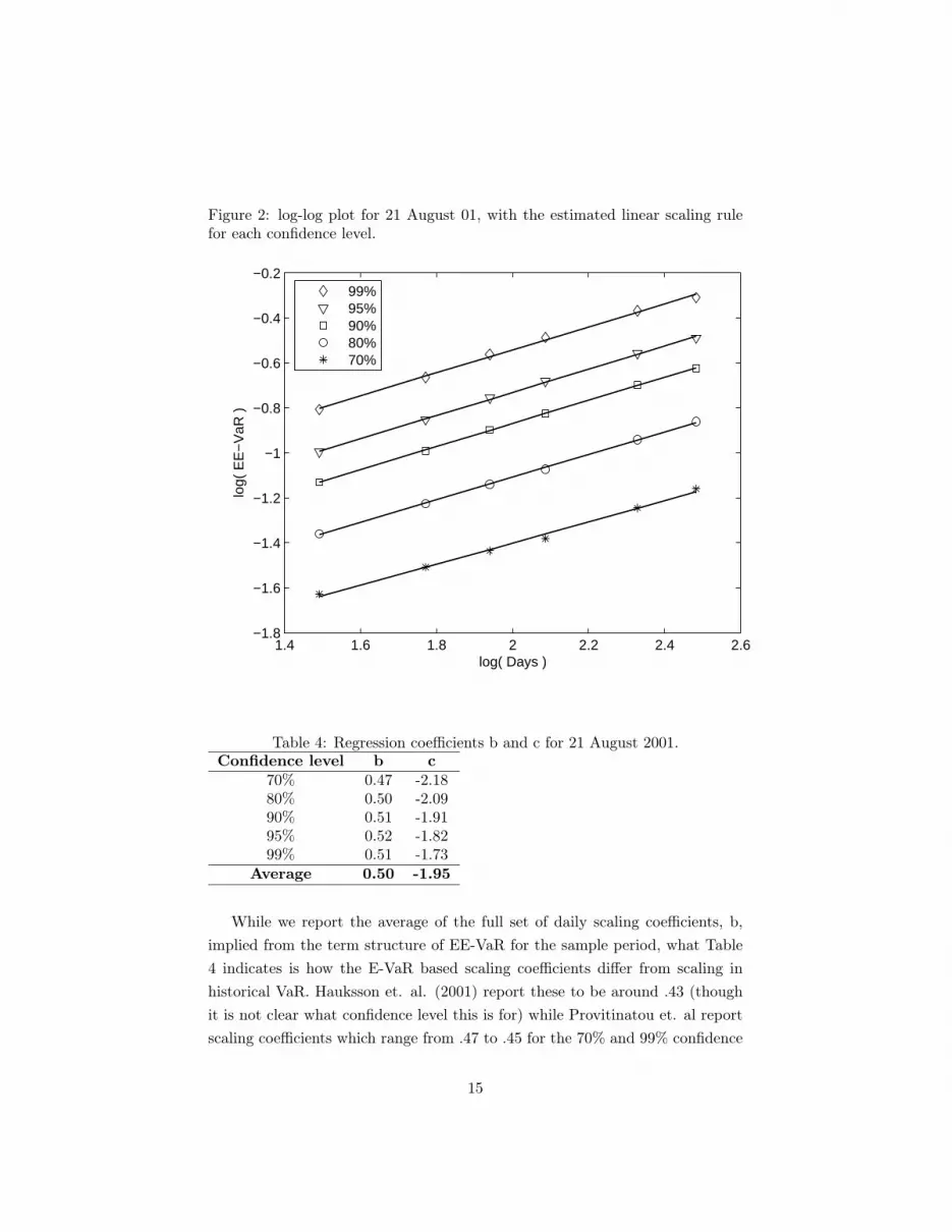
Figure 2: log-log plot for 21 August 01, with the estimated linear scaling rulefor each confidence level.

1.4 1.6 1.8 2 2.2 2.4 2.6−1.8

−1.6

−1.4

−1.2

−1

−0.8

−0.6

−0.4

−0.2

log( Days )

log(

EE

−V

aR )

99%95%90%80%70%

Table 4: Regression coefficients b and c for 21 August 2001.Confidence level b c

70% 0.47 -2.1880% 0.50 -2.0990% 0.51 -1.9195% 0.52 -1.8299% 0.51 -1.73

Average 0.50 -1.95

While we report the average of the full set of daily scaling coefficients, b,implied from the term structure of EE-VaR for the sample period, what Table4 indicates is how the E-VaR based scaling coefficients differ from scaling inhistorical VaR. Hauksson et. al. (2001) report these to be around .43 (thoughit is not clear what confidence level this is for) while Provitinatou et. al reportscaling coefficients which range from .47 to .45 for the 70% and 99% confidence

15

levels, respectively. As will be seen, in general the market implied VaR scalesmore vigorously with time at higher quantiles. However, the size of the scalingcoefficients in Tables 4 and 5 should not be confused with implying unboundedsecond and higher moments of the RND functions as the implied tail parametersξ at all times for the sample period showed that up to 4 moments exist.

4.3 Improving the estimation of the linear scaling law byusing WLS

The linear regression estimated to obtain the time scaling for EE-VaR canbe affected by EE-VaR values calculated from an RND constructed from veryfew option prices. The EE-VaR estimates in such cases will have very wideconfidence intervals. As an example, take the data and regression for 12 Nov97, shown in Figure 3 below. The R2 of the OLS regression was 64.8%, a verypoor fit. The EE-VaR value furthest away from maturity was obtained froman RND estimated using only 4 option prices, and thus the confidence intervalsof the EE-VaR estimate are much wider than the EE-VaR values obtained forcloser maturities, which are based on RNDs extracted using around 25 contracts.

One method to solve this issue is to use a Weighted Linear Squares (WLS)regression, using the number of option prices available at each maturity relativeto total prices as weights for the EE-VaR values.

WeightedR2 = 1−∑TN

i=T1wi (yi − yi)

2∑TN

i=T1wi (yi − yi)

2, with

TN∑i=T1

wi = 1, (16)

wi =NumberOfPriceAtMaturityi

TotalNumberOfPrices(17)

Table 5: Average R2 for different quantiles, and number of days with differentranges of R2

Confidence level 70% 80% 90% 95% 99%Average R2 87.9% 97.9% 98.8% 98.7% 97.9%

Number of days with R2 > 99% 429 1152 1410 1320 90199% ≥ R2 > 90% 860 510 282 375 742

R2 ≤ 90% 444 71 41 38 90

Table 6 below shows the average weighted R2 at each confidence level. Notehow the fitting performance increases with confidence level, while it is lowest at96.8% for the lowest quantile of 70%.

16

Figure 3: Example of linear regression using OLS vs. WLS for a day when thereare some maturities with very few option prices available.

Table 6: Average weighted R2 at each quantileConfidence level 70% 80% 90% 95% 99%

Weighted R2 96.8% 99.4% 99.6% 99.5% 99.3%

4.4 Full Regression results for scaling in EE-VaR

The average regression coefficients b and c across the 1733 days in our sampleperiod are displayed in Table 7 below. We can see that the slope b increaseswith the confidence interval, and that intercept, i.e. the 1 day EE-VaR alsoincreases with confidence level, as one would expect. The standard deviation ofthe estimates at different confidence levels is fairly constant. We also report thepercentage number of days where b was found to be statistically significantlydifferent from one half.12 On average, irrespective of the confidence level, we

12Newey-West (1987) heterosckedasticity and autocorrelation consistent standard error was

17

found that in around 50% of the days the scaling was significantly different than0.5, the scaling implied by the square root of time rule.

Table 7: Average regression coefficients b,c and exp(c) across the 1733 days inthe sample, for the GEV case. #: The percentage number of days where b wasstatistically significantly different from 0.5. †: Standard deviation of bConfidence level q b(q) c EVaR(1,q) = exp(c)

0.41 -2.2470% (51.3%)# (0.26)† 0.6%

(0.12)† level0.48 -2.04

80% (51.1%)# (0.23)† 0.9%(0.09)†0.51 -1.84

90% (52.4%)# (0.23)† 1.4%(0.09)†0.53 -1.73

95% (52.1%)# (0.23)† 1.9%(0.09)†0.56 -1.57

99% (52.6%)# (0.25)† 2.7%(0.11)†

-1.88

Figure 4 displays the time series of the b estimates (the slope of the scalinglaw) for the GEV case at the 95% confidence level. Even though the averagevalue of b at this confidence level is 0.53 (see Table 7), it appears to be timevarying and takes values that range from 0.2 to 1.

used to test the null hypothesis H0 :b = 0.5. We employed this methodology when testing thestatistical significance of the estimated slope b, because E-VaR estimates are for overlappinghorizons, and therefore are auto-correlated. The Newey-West lag adjustment used was n - 1.

18

Figure 4: Time series of b estimates for the GEV model at 95% confidence

4.5 Comparison of EE-VaR with other models for E-VaR

Figure 5 below displays the time series of 90 day EVaR estimates at the 95%confidence level for each of the three parametric methods for RND extraction(combined with their respective empirical scaling regression results) togetherwith the estimates from the Bank of England non-parametric method. The 90day FTSE returns are also displayed in Figure 5.

Table 8 below shows the sample mean and standard deviation of each of thefour EVaR time series. If we use the BoE values as the benchmark, we cansee that on average, the mixture of lognormals method overestimates EVaR,while the Black-Scholes method underestimates it. Among the three parametricmethods, the GEV method yields the time series of EVaRs closest to the BoEone. This can be seen both from Table 8 and also in the Figure 5, where theBoE time series practically overlaps the GEV E-VaR time series. This confirmsthat the GEV based VaR calculation is equivalent to the semi-parametric oneused by the Bank of England but also has the added advantage, as we will seein the next section, of being capable of providing 10 day E-VaRs at the industrystandard 99% confidence level.

19

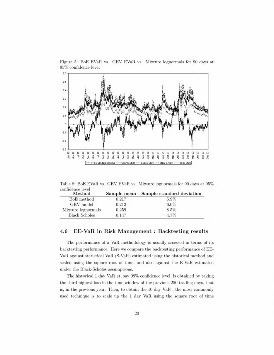
Figure 5: BoE EVaR vs. GEV EVaR vs. Mixture lognormals for 90 days at95% confidence level

Table 8: BoE EVaR vs. GEV EVaR vs. Mixture lognormals for 90 days at 95%confidence level

Method Sample mean Sample standard deviationBoE method 0.217 5.9%GEV model 0.212 6.0%

Mixture lognormals 0.259 8.5%Black Scholes 0.147 4.7%

4.6 EE-VaR in Risk Management : Backtesting results

The performance of a VaR methodology is usually assessed in terms of itsbacktesting performance. Here we compare the backtesting performance of EE-VaR against statistical VaR (S-VaR) estimated using the historical method andscaled using the square root of time, and also against the E-VaR estimatedunder the Black-Scholes assumptions.

The historical 1 day VaR at, say 99% confidence level, is obtained by takingthe third highest loss in the time window of the previous 250 trading days, thatis, in the previous year. Then, to obtain the 10 day VaR , the most commonlyused technique is to scale up the 1 day VaR using the square root of time

20

rule. The percentage number of violations at each confidence level q needs tobe below the benchmark (1-q). For example, at the 99% confidence level, thepercentage of days where the predicted VaR is exceeded by the market shouldbe 1%. If there are fewer violations than the benchmark 1%, it means thatthe VaR estimate is too conservative, and it could impose an excessive capitalrequirement for the banks. On the other hand, if there are more violations thanthe benchmark 1%, the VaR estimates are too low, and the capital set aside bythe bank would be insufficient.

We use our method to calculate the GEV and Black-Scholes based E-VaRvalues at constant time horizons of 1, 10, 30, 60, and 90 days. Tables 9, 10and 11 show the results in terms of percentage number of violations for EE-VaR, S-VaR, and Black-Scholes E-VaR, respectively. The values highlightedin bold indicate that the benchmark percentage number of violations has beenexceeded. On the other hand, the non highlighted values indicate that thebenchmark percentage number of violations at the given confidence level hasnot been exceeded. The last row of each table displays the average percentagenumber of violations across maturities for each confidence level. In the rowlabelled “Benchmark” we can see the target percentage number of observationsat each confidence level.

We can see that of all the three methods, EE-VaR yields the least numberof cases where the benchmark percentage violations is exceeded. However, itexceeds the benchmark at all confidence levels for the 1 day horizon. The S-VaRalso exceeds the benchmark at all confidence levels for the 1 day horizon, butadditionally, it exceeds it for the 10 day horizon at 97% and 99% confidencelevels, and for the 30 day horizon at almost all confidence levels. The Black-Scholes based E-VaR is the worst of all methods, exceeding the benchmark in14 out of the 25 cases.

Looking at the averages across horizons for the three methods, we see thatEE-VaR and S-VaR yield similar results at the higher quantiles (98% and 99%),but EE-VaR appears further away from the benchmark than S-VaR at the otherconfidence levels, indicating that it may be too conservative. On average, theBlack-Scholes based E-VaR exceeds the benchmark percentage number of viola-tions at all but the lowest confidence level, which indicates that it substantiallyunderestimates the probability of downward movements at high confidence lev-els.

21

Table 9: Percentage violations of EE-VaRHorizon Confi- level

dence(days) 95% 96% 97% 98% 99%

Benchmark 5% 4% 3% 2% 1%1 6.2% 5.5% 4.4% 3.8% 3.1%10 2.4% 1.8% 1.5% 1.3% 0.6%30 2.8% 2.0% 1.3% 0.5% 0.1%60 2.5% 2.2% 1.3% 0.7% 0.0%90 2.9% 2.3% 1.5% 0.8% 0.0%

Average 3.4% 2.8% 2.0% 1.4% 0.8%

Table 10: Percentage violations of Statistical VaR (S-VaR)Horizon Confi- level

dence(days) 95% 96% 97% 98% 99%

Benchmark 5% 4% 3% 2% 1%1 5.9% 4.7% 3.8% 2.5% 1.5%10 4.6% 4.0% 3.1% 1.7% 1.4%30 5.3% 4.2% 3.3% 2.1% 0.8%60 4.3% 3.6% 2.8% 1.1% 0.3%90 4.5% 2.8% 1.9% 0.7% 0.0%

Average 4.9% 3.9% 3.0% 1.6% 0.8%

Table 11: Percentage violations of Black-Scholes based E-VaRHorizon Confi- level

dence(days) 95% 96% 97% 98% 99%

Benchmark 5% 4% 3% 2% 1%1 6.8% 5.9% 5.1% 4.4% 3.5%10 3.6% 3.2% 2.3% 2.0% 1.0%30 4.0% 3.8% 3.3% 2.4% 1.3%60 3.9% 3.3% 2.9% 2.4% 1.7%90 4.6% 4.1% 3.7% 3.0% 2.0%

Average 4.6% 4.1% 3.5% 2.8% 1.9%

Figure 6 below shows the time series of 10 day FTSE returns, 10 day EE-VaRand 10 day S-VaR, both at 99% confidence level. We have chosen to plot theVaR of these particular set of (q, k) values as the 10 day VaR at 99% confidencelevel is one of most relevant VaR measures for practitioners, given the regulatory

22

reporting requirements. We can see how the S-VaR is violated more times (25times, or 1.4% of the time) than the EE-VaR (10 times, or 0.6%) by the 10 dayFTSE return.

Figure 6: Time series of the 10 day FTSE returns, 10 day EE-VaR and 10 dayS-VaR, both at a 99% confidence level.

4.7 E-VaR vs. Historic VaR x3

The Basle Committee on Banking Supervision explains in the “Overviewof the Amendment to the Capital Accord to Incorporate Market Risks” (1996)that the multiplication factor, ranging from 3 to 4 depending on the backtestingresults of a bank’s internal model, is needed to translate the daily value-at-riskestimate into a capital charge that provides a sufficient cushion for cumulativelosses arising from adverse market conditions over an extended period of time.But it is also designed to account for potential weaknesses in the modellingprocess. Such weaknesses exist because:

• Market price movements often display patterns (such as "fat tails") thatdiffer from the statistical simplifications used in modelling (such as theassumption of a "normal distribution").

• The past is not always a good approximation of the future (for example

23

volatilities and correlations can change abruptly).

• VaR estimates are typically based on end-of-day positions and generallydo not take account of intra-day trading risk.

• Models cannot adequately capture event risk arising from exceptional mar-ket circumstances.

It is interesting to note from Figure 7 that the E-VaR values in periods of marketturbulence (Asian Crisis, LTCM crisis and 9/11) are similar to the historical S-VaR values when multiplied by a factor of 3. Thus, the multiplication factor 3for a 10 day S-VaR appears to justify the reasoning that it will cover extremeevents. In contrast, as we are modelling extreme events explicitly under EE-VaRsuch ad hoc multiplication factors are unnecessary.

Figure 7: 10 day at 99% E-VaR vs. Statistical VaR multiplied by a factor of 3

4.8 Capital requirements

The average capital requirement based on the EE-VaR, S-VaR and S-VaRx3for the 10 day VaR at different confidence level is displayed in Table 12 below.

24

Here, the capital requirement is calculated as a percentage of the value of aportfolio that replicates the FTSE 100 index. What is very clear is that EE-VaRwhen compared to S-VaRx3 shows substantial savings in risk capital, needingonly on average 1.7% more than S-VaR to give cover for extreme events. S-VaRx3 needs over 2.36 times as much capital for risk cover at 99% level. Figure7 clearly gives the main draw back of historically derived VaR estimates wherethe impact of large losses in the past result in high VaR for some 250 days ata time. The EE-VaR estimates are more adept at incorporating market datainformation contemporaneously.

Table 12: Average daily capital requirement based on a 10 day horizon at dif-ferent confidence levels, with standard deviations in brackets.

Confi- level Aver-dence age

95% 96% 97% 98% 99%S- 6.5% 7.3% 7.8% 9.1% 10.1% 8.2%

VaR (1.9%) (2.3%) (2.4%) (2.9%) (2.8%) (2.5%)S-VaR 19.5% 21.9% 23.4% 27.3% 30.3% 24.48%×3 (5.7%) (6.9%) (7.2%) (8.7%) (8.4%) (7.38%)EE- 8.1% 8.7% 9.6% 10.8% 12.7% 9.9%VaR (3.1%) (3.3%) (3.7%) (4.2%) (5.0%) (3.9%)

5 Conclusions

We propose a new risk measure, Extreme Economic Value at Risk (EE-VaR), which is calculated from an implied risk neutral density that is based onthe Generalized Extreme Value (GEV) distribution. In order to overcome theproblem of maturity effect, arising from the fixed expiration of options, we havedeveloped a new methodology to estimate a constant time horizon EE-VaR byderiving an empirical scaling law in the quantile space based on a term structureof RNDs. Remarkably, the Bank of England semi-parametric method for RNDextraction and the constant horizon implied quantile values estimated daily for a90 day horizon coincides closely with the EE-VaR values at 95% confidence levelshowing that GEV model is flexible enough to avoid model error displayed by theBlack-Scholes and Mixture of Lognormal models. The main difference betweenthe Bank’s method and the one that relies on an empirical linear scaling lawof the E-VaR based on a daily term structure of the GEV RND is that shorterthan 1 month E-VaRs and in particular daily 10 day E-VaR can be reported

25

in our framework. This generally remains problematic in the RND extractionmethod based on the implied volatility surface in delta space as it is non-linearin time to maturity and also it cannot reliably report E-VaR for high confidencelevels of 99%.

Based on the backtesting and capital requirement results, it is clear thereis a trade-off between the frequency of benchmark violations of the VaR value,and the amount of capital required. The 10 day EE-VaR gives fewer cases ofbenchmark violations, but yields higher capital requirements compared to the10 day S-VaR. However, when the latter is corrected by a multiplication factorof 3, to satisfy the violation bound, the risk capital needed is more that 2.3times as much as EE-VaR for the same cover at extreme events. This savingin risk capital with EE-VaR at high confidence levels of 99% arises because animplied VaR estimate responds quickly to market events and in some cases evenanticipate them.

While the power of such a market implied risk measure is clear, both asan additional tool for risk management to estimate the likelihood of extremeoutcomes and for maintaining adequate risk cover, the EE-VaR needs furthertesting against other market implied parametric models as well as S-VaR meth-ods. This will be undertaken in future work.

References[1] Ait-Sahalia, Y., Lo, A.W., (2000). “Nonparametric risk management and

implied risk aversion”. Journal of Econometrics 94, 9–51.

[2] Ait-Sahalia, Y., Wang, Y., Yared, F., (2001) “Do option markets correctlyprice the probabilities of movement of the underlying asset?” Journal ofEconometrics 102, 67–110.

[3] Alentorn, A. (2007) Option Pricing with the Generalized Extreme ValueDistribution and Applications, PhD thesis, University of Essex.

[4] Alentorn, A., Markose, S. (2006) “Removing Maturity Effects of ImpliedRisk Neutral Densities and Related Statistics”, University of Essex, De-partment of Economics Discussion Paper, Number 609.

[5] Anagnou, I., Bedendo, M., Hodges, S D. and Tompkins, R. G., (2002)"The Relation Between Implied and Realised Probability Density Func-tions" EFA 2002 Berlin Meetings Presented Paper; University of WarwickFinancial Options Research Centre Working Paper.

[6] Bates, D.S., (1991). “The Crash of ’87: Was it expected? The evidencefrom options market”. Journal of Finance 46, 1009–1044.

26

[7] Bali, T. G. (2003). “The generalized extreme value distribution”. EconomicsLetters 79, 423-427.

[8] Black, F. and M. Scholes (1973). “The Pricing of Options and CorporateLiabilities”. Journal of Political Economy 81, 637-659.

[9] Clews, R., Panigirtzoglou, N., Proudman, J., (2000). “Recent developmentsin extracting information from option markets.” Bank of England QuarterlyBulletin 40, 50–60.

[10] Cont, R. (2001): “Empirical properties of asset returns: stylized facts andstatistical issues”. Quantitative Finance 1.

[11] Cont, R. and de Fonseca, J. (2002) “Dynamics of implied volatility sur-faces”. Quantitative Finance 2 45-60.

[12] Danielsson, J. and J. Zigrand ( 2004). "On time-scaling of risk and thesquare-root-of-time rule." FMG Discussion Papers. Discussion Paper Num-ber 439.

[13] Danielsson, J. and C.G. de Vries (1997) “Tail index estimation with veryhigh frequency data”, Journal of Empirical Finance, 4, 241-257.

[14] De Haan, L., D.W. Cansen, K. Koedijk and C.G. de Vries (1994) “Safetyfirst portfolio selection, extreme value theory and long run asset risks. Ex-treme value theory and applications” (J. Galambos et al., eds.) 471-487.Kluwer, Dordrecht.

[15] Dowd, K. (2002). Measuring Market Risk. Wiley Press.

[17] Dacorogna, M. M., Müller, U. A., Pictet, O. V., de Vries, C. G. (2001)“Extremal Forex Returns in Extremely Large Data Sets”, Extremes, 4,105-127.

[18] Dumas, B., Fleming, J. and Whalley, R.E., (1998), “Implied VolatilityFunctions: Empirical Tests”, Journal of Finance, Volume 53, No. 6, pp.2059-2106.

[19] Embrechts, P., C. Klüppelberg and T. Mikosch (1997) Modelling ExtremalEvents for Insurance and Finance. Berlin: Springer.

[20] Embrechts P., S. Resnick and G. Samorodnitsky (1999). “Extreme valuetheory as a risk management tool” North American Actuarial Journal 3,30-41.

[21] Embrechts, P. (2000) “Extreme Value Theory: Potential and Limitationsas an Integrated Risk Management Tool” Derivatives Use, Trading & Reg-ulation, 6, 449-456.

[22] Fama, E. (1965). "The behaviour of stock market prices." Journal of Busi-ness. 38. 34-105.

27

[23] Gemmill G, and A. Saflekos (2000) “How Useful are Implied Distributions?Evidence from Stock-Index Options” Journal of Derivatives 7, 83-98.

[24] Hardle, W. and Hlavka, Z. (2005) “ Dynamics of State Price Densities”.SFB 649 Discussion Paper 2005-021.

[25] Hauksson, H.A, M. Dacorogna, T. Domenig, U. Müller, and G. Samorod-nitsky, (2001), “Multivariate extremes, aggregation, and risk estimation”,Quantitative Finance 1:79-95.

[26] Jackwerth, J. C. (1999). “Option-Implied Risk-Neutral Distributions andImplied Binomial Trees: A Literature Review”. The Journal of Derivatives,7, 66-82.

[27] Kaufmann, R. and P. Patie (2003). "Strategic Long-Term Financial Risks:The One-Dimensional Case." RiskLab Report. (ETH Zurich).

[28] Mandelbrot, B. (1963). "The Stable Paretian Income Distribution whenthe Apparent Exponent is Near Two." International Economic Review. 4.(1). 111-115.

[29] Mandelbrot, B. (1967). "The Variation of Some Other Speculative Prices."Journal of Business. 40. 393-413.

[30] Markose, S. and Alentorn, A. (2005). “The Generalized Extreme Value(GEV) Distribution, Implied Tail Index and Option Pricing”. Universityof Essex, Department of Economics Discussion Paper, Number 594. Underrevision with Journal of Derivatives.

[31] Melick, W. R. (1999). “Results of the estimation of implied PDFs from acommon data set”. Proceedings of the Bank for International SettlementsWorkshop on ‘Estimating and Interpreting Probability Density Functions’,Basel, Switzerland.

[32] Melick, W. R. and C. P. Thomas (1998). “Confidence intervals and constantmaturity series for probability measures extracted from option prices”, Pa-per presented at the conference ‘Information contained in Prices of Finan-cial Assets’, Bank of Canada.

[33] Melick, W. R. and C. P. Thomas (1996). “Using Option prices to infer PDFsfor asset Prices: An application to oil prices during the Gulf war crisis”.International Finance Discussion Paper, No. 541, Board of Governors ofthe Federal Reserve System.

[34] Menkens, O. (2004). “Value-at-Risk and Self Similarity”. Mimeo. Centre forComputational Finance and Economic Agents, University of Essex, UK.

[35] McNeil, A.J. and R. Frey. (2000). “Estimation of tail-related risk measuresfor heteroscedastic financial time series: an extreme value approach”. Jour-nal of Empirical Finance. 7: 271-300.

28

[36] Ncube, M. (1996) “Modelling implied volatility with OLS and panel datamodels”, Journal of Banking and Finance, 20, 71-84.

[37] Panigirtzoglou, N. and G. Skiadopoulos (2004) “A New Approach to Mod-elling the Dynamics of Implied Distributions: Theory and Evidence fromthe S&P 500 Options” Journal of Banking and Finance, 28, 1499-1520.

[38] Provizionatou, V., S. Markose and O. Menkens (2005) “Empirical ScalingLaws In VaR ”, Mimeo, Centre for Computational Finance and EconomicAgents, University of Essex, UK.

[39] Ritchey, R. J. (1990) “Call Option Valuation for Discrete Normal Mixtures”.Journal of Financial Research, 13, 285-296.

[40] Shiratsuka, S. (2001) “Information Content of Implied Probability Distri-butions: Empirical Studies on Japanese Stock Price Index Options”, IMESDiscussion Paper 2001-E-1, Institute for Monetary and Economic Studies,Bank of Japan.

29