introduction to matlab 1 0
TRANSCRIPT

,QWURGXFWLRQ�WR�0DWODEDept. Zoology and Neurobiology
Ruhr University Bochum1999
Bart Krekelberg
Version 1.0 - March 1999
Current Address:[email protected]

�
�� 7DEOH�RI�&RQWHQWV�
1 Table of Contents........................................................................................ 3
2 Introduction .................................................................................................. 7
3 Basics........................................................................................................... 9
3.1 Variables.......................................................................................... 9
3.2 Vectors and Matrices.................................................................... 11
3.2.1 Addition...................................................................................... 13
3.2.2 Subtraction ................................................................................ 13
3.2.3 Multiplication.............................................................................. 13
3.2.4 Division ...................................................................................... 14
3.2.5 Powers....................................................................................... 14
3.2.6 Matrix Operation........................................................................ 14
3.3 Special Matrices............................................................................ 15
3.3.1 Zeros.......................................................................................... 15
3.3.2 Ones .......................................................................................... 15
3.3.3 Meshgrids.................................................................................. 16
3.4 Matrix Manipulation....................................................................... 16
3.4.1 Subscript Addressing................................................................ 16
3.4.2 Index Addressing ...................................................................... 18
3.4.3 Logical Addressing.................................................................... 18
3.5 Matrix Functions............................................................................ 20
3.5.1 find ............................................................................................. 20
3.5.2 size, length ................................................................................ 21
3.5.3 flipud, fliplr.................................................................................. 21
3.5.4 Reshape, [ ], : ............................................................................ 21
3.6 General Mathematics ................................................................... 22
3.7 Further Reading ............................................................................ 22
3.8 Excercises..................................................................................... 23
INTRODUCTION TO MATLAB
�
4 Strings ........................................................................................................ 25
4.1 Manipulating strings...................................................................... 25
4.2 String Cell Arrays .......................................................................... 27
4.3 Further Reading ............................................................................ 27
4.4 Excercises..................................................................................... 27
5 Programming............................................................................................. 29
5.1 Flexible Functions......................................................................... 32
5.2 Flow Control .................................................................................. 34
5.2.1 for x = vector ... end ................................................................. 35
5.2.2 while a<b end............................................................................ 36
5.2.3 if a<b end................................................................................... 37
5.2.4 switch case end......................................................................... 37
5.3 Error Handling ............................................................................... 38
5.4 Miscellaneous Programming Tricks............................................. 38
5.4.1 Programming with eval ............................................................. 38
5.5 Using large arrays......................................................................... 39
5.6 Further Reading ............................................................................ 39
5.7 Exercises....................................................................................... 40
6 Graphics..................................................................................................... 41
6.1 Two Dimensional Plots................................................................. 41
6.2 Special Two Dimensional Plots.................................................... 45
6.2.1 Polar Plots ................................................................................. 45
6.2.2 Bar Charts ................................................................................. 45
6.2.3 Histograms. ............................................................................... 47
6.2.4 Arrow Plots (Compass, Feather, Quiver) ................................ 49
6.3 Three Dimensional Plots .............................................................. 51
6.4 Fine Tuning ................................................................................... 54
6.5 Printing and Exporting Graphics .................................................. 61
6.5.1 Latex .......................................................................................... 61
TABLE OF CONTENTS
�
6.5.2 Word / PowerPoint.................................................................... 61
6.6 Further Reading ............................................................................ 62
6.7 Excercises..................................................................................... 62
7 Data Analysis............................................................................................. 63
7.1 Statistics ........................................................................................ 63
7.2 Correlations................................................................................... 64
7.3 Fourier Analysis ............................................................................ 65
7.4 Data smoothing............................................................................. 65
7.5 Optimization .................................................................................. 66
7.6 Curve Fitting.................................................................................. 66
7.7 Excercises..................................................................................... 67
8 FileIO.......................................................................................................... 69
8.1 Storing Matlab Results ................................................................. 69
8.1.1 Data ........................................................................................... 69
8.1.2 Figures....................................................................................... 69
8.2 Importing Data............................................................................... 69
8.3 Exporting Data .............................................................................. 70
8.3.1 Excel .......................................................................................... 71
8.4 Excercises..................................................................................... 71
9 Datastructures and Object Oriented Programming ................................ 72
9.1 N-dimensional Arrays ................................................................... 72
9.2 Structures ...................................................................................... 73
9.3 Classes and Object-Oriented Programming ............................... 74
9.3.1 The constructor ......................................................................... 75
9.3.2 Class Methods .......................................................................... 76
9.3.3 Overloading Methods ............................................................... 77
9.3.4 Reading and Writing Object Properties ................................... 79
9.3.5 Caveats and Comments........................................................... 81
9.4 Exercises....................................................................................... 82

INTRODUCTION TO MATLAB
�
10 GUI Building.................................................................................. 83
10.1 Graphical Design with Guide........................................................ 83
10.1.1 Setting the Properties ............................................................... 84
10.2 Programming Callbacks ............................................................... 84
10.3 Reading the Settings .................................................................... 85
10.4 Dealing with data .......................................................................... 87
10.5 Further Reading ............................................................................ 87
10.6 Exercises....................................................................................... 87
11 Miscellaneous ............................................................................... 89
11.1 Help ............................................................................................... 89
11.1.1 Looking for Help........................................................................ 89
11.1.2 Providing Help........................................................................... 89
11.2 Debugger....................................................................................... 89
11.3 Profiler ........................................................................................... 90
11.4 Public Tools................................................................................... 90
11.5 Network Use.................................................................................. 91
11.6 Operating System Issues ............................................................. 91
12 Answers to Selected Exercises.................................................. 93
12.1 Comments..................................................................................... 93
12.2 Basics ............................................................................................ 93
12.3 Strings............................................................................................ 95
12.4 Programming................................................................................. 95
12.5 Graphics ........................................................................................ 97
12.6 Data Analysis ................................................................................ 99
�
�� ,QWURGXFWLRQ�
The Matlab environment and programming language is used in a wide range of scientific applications. These vary from the design of controllers for the precision landing of an airplane (Daimler Benz), forecasting of financial products (Lionhart Investments) to the analysis of cardiac arythmia in sheep (Washington University). In neuroscience, Matlab’s use is increasing due to the higher demands put on data analysis by modern recording techniques, but also the higer demands put on the quality of visualisation. In the department, Matlab is used extenisvely for the analysis of both physiological and psychophysical data. If all you want to do is to determine the average and standard deviation of a small set of reaction times, use a calculator, or Excel if you need graphs too. If, however, you want to fit complicated non-linear models to your response curves, analyse spike times to generate peri-stimulus time histograms and corresponding polar tuning curves, or even to analyse the signals coming from an fMRI equipment, use Matlab. Matlab is a programming language especially suited for the numerical analysis of data. Users can define complex algorithms themselves, or use one of the many pre-defined routines. Usually a Matlab program will consist of a combination of the two. It is therefore good to learn not only the structure of the programming language, but also to find out what kind of functions for analysis have already been implemented in Matlab. The help files (in PDF or HTML format) are very extensive and everyone should browse through them from time to time. More information on the use of Help is given in section 11.1. Apart from the built-in functions, Matlab has Toolboxes. These are packages that define additional functions in a specific area. Currently, our department has a Matlab 5.2 license for the Neural Networks Toolbox, the Signal Processing Toolbox, and the Optimization Toolbox. The most directly relevant functions of those toolboxes are described in this document, but browse the (online-) documentation for more details. A third source of pre-defined functions is the collection of user-contributed M-files at the Matlab world-wide-web site. (http://www.mathworks.com/ or http://www-europe.mathworks.com/) These are functions and sometimes extensive programs contributed by Matlab users. They are free to download and use, but obviously come without any warranty. They are written by people by you and me, and hence they will contain bugs. I do recommend using these, but never without some testing or without having a look at the source code to check what the program does. Further sources of information on the Mathworks homepage are the Solution Search Engine, which is a database of frequently asked questions that can be searched for keywords. This is extremely useful if you are stuck in some programming problem. The Matlab Access program (Username Krekelberg, Access number 133196) provides a further layer of information. The most interesting documents are the short courses in various subjects. Browse the Mathworks site from time to time to keep your Matlab knowledge up-to-date. A fourth source of pre-defined functions is a collection of Matlab scripts written by people in the department. These files are stored on the server in \public\matlab. A listing of their functionality is provided in section 11.4. The same warning applies here: if you use a program, you are responsible for its proper behaviour, not the author. Test it. If you write a program that may have applicability beyond your analysis, please save others some time and add it to the archive. Before doing so, add comments to the code and describe the usage of the program in the first lines of the file (see section 11.1.2). If none of the above sources can provide you with a solution, you will have to program it yourself. This book will help you get started in writing Matlab programs. In section 3 I will discuss the basic building blocks of all Matlab programs. These are vectors and matrices and the way in which they can be manipulated with fast, vector functions. Specific programming tricks to execute the same action on many datasets (loops) or to execute different actions on many datasets (conditionals) are discussed in section 5.2. When the anaysis is done, you will want to see the result in a visually attractive way. Matlab has a large repertoire of methods to visualise data. Two-dimensional cartesian plots, three-dimensional plots, colour coding, contour plots, and ways to personalise your graphs are presented in section 6. Section 7 is concerned with built-in Matlab functions that are particularly useful for the analysis of (neuroscience) data. Curve fitting, cross-correlation and statistical significance tests are just a few of the possibilities. Section 8 demonstrates how to load datafiles from other programs for analysis in Matlab and how to save your results or export them to other programs for post-processing.
INTRODUCTION TO MATLAB
�
More advanced programming techniques, including the highly recommended object oriented methods, are discussed in section 9. Whenever you want to explore your data with many different data analysis methods, it may be worth developing a graphical user interface (GUI) for your analysis. A (good) GUI makes it easy to change parameters of your analysis (think for instance of bin-width, averaging window, median or mean as a method for averaging, etc.) and immediately shows the results that this change has on your data. Moreover, it should also be easy to load a new dataset (a different cell, or another subject) and immediately see the results of the analysis of this dataset. Building a GUI has been much simplified with the introduction of GUIDE (GUI-Development Environment) with Matlab 5, but is still not for the fainthearted. An introduction, tips and caveats are presented in section 1. Finally, in section 11 I discuss miscellaneous items such as the extensive help facilities, the debugger etc. Just reading this introduction to Matlab may teach you the basics of programming in Matlab, but you will not become a master of data analysis overnight. The most important thing will be to practice the newly acquired knowledge. The exercises allow you to test your ability to use the knowledge you acquired in a particular chapter. Try coming up with your own solution before looking at some of the suggestions for a solution in section 11.5. If you want to improve your skills beyond what you can learn from this book, the ’Further Reading’ sections point to additional information available in the Help files, the on-line documentation or on the World Wide Web.

�
�� %DVLFV�
The Matlab program is started by clicking the Matlab icon in your start menu or by clicking the Matlab executable in the \Bin subdirectory of the Matlab directory tree. This is usually found under c:\Program Files\Matlab\Bin. Starting the program gives you white screen with a few comments about how to get started and the prompt ’>>’ waiting for your input. The Matlab menubar, at the top of the screen, has four sub-menus. The File menu allows you to save a Matlab session, to print data or a figure, and to set various options concerning the operation of Matlab (under Preferences). The details of the function of these options will be discussed later. In the Edit menu you can cut, copy and paste parts of the command window, just as if the Command window were an ordinary text editor. The Window menu allows you to switch between the various figures that are related to your Matlab session, such as figures, control panels and the editor/debugger. The Help submenu, finally, gives access to the extensive Help facilities of Matlab. You enter commands by typing them at the command prompt. At the prompt you can perform calculations as in a normal calculator, but also assign the results of calculations to variables, as in a programming language. All mathematical functions of a scientific calculator are available For example*: exp(10) sin(0) ans = 2.2026e+004 ans = 0 Of course you will want to use Matlab for more than a fancy calculator. The basis for this is the use of variables. Their definition is explained in the next section.
���� 9DULDEOHV�
Variables are the memory of Matlab (or any other programming language). Variables allow you to store intermediate results of your calculations for later use. For instance: a=exp(10) a = 2.2026e+004 stores the result of the simple calculation exp(10) in the variable with the name a. In a subsequent calculation, you can now use the variable name a to refer to the number 2.2026e+004. Hence: log(a) ans = 10 Variable names in Matlab can be arbitrarily long, should contain only alphanumeric characters and are case-sensitive. Be careful not to redefine one of the Matlab commands as a variable. Matlab will not express any warnings when you type: print =2 print = 2
* Examples of Matlab code are interleaved with the text. The font (Courier Bold) distinguishes code from text. Matlab’s response to a line of code is shown in normal Courier.
INTRODUCTION TO MATLAB
���
but afterwards, you will not be able to use the print command anymore: in response to print, Matlab will just return the contents of the variable print, rather than executing the command print. The variable with the name ’ans’, short for answer, is a special variable that contains the result of the last calculation at the command prompt, which was not assigned to a variable. In other words, if you enter a mathematical command at the command prompt without specifying a variable for the result, Matlab automatically assigns the result to the variable ans. For instance, sqrt(99) ans = 9.9499 Just as a variable you define, ans can be used in further calculations: ans*ans ans = 99 If variables could only contain numbers, their use would be limited. In Matlab a variable can contain just about anything: a list of numbers (i.e. a vector), a bit of text (i.e. a string), or even a complex, but not arbitrary combination of text and numbers: times = [ 10 20 30 40] times = 10 20 30 40 The variable times now contains the 4 values 10, 20, 30 and 40 that may be relevant to an analysis. Variables can be thought of as boxes containing data. These can be raw data, acquired from some data-recording program, but also processed data, which are the result of a Matlab calculation with raw data. Another way of looking at variables is to think of them as the name or address of a chunk of data. Hence, the variable times tells Matlab where to look for those particular numbers that play a role in our data analysis. The variables you define, plus those that Matlab defines, are stored in something called the Matlab workspace. When you start Matlab, a default empty workspace is created. To view the contents of this workspace, type who for a brief description or whos for a listing that includes the sizes and formats of the variables. whos Name Size Bytes Class a 1x1 8 double array ans 1x1 8 double array print 1x1 8 double array times 1x4 32 double array Grand total is 7 elements using 56 bytes This tells us that we have three defined variables, the first, a, is the one that was defined first, it contains the result of the calculation exp(10). Matlab uses 8 bytes to store this value with double precision. The ’class’ of this variable is ’array’, which means it contains simple numerical values. About the times variable, Matlab tells us that it is of a size 1*4, which means that it contains one row of four elements (which we know to be the numbers 10, 20, 30 and 40). In Matlab memory storing the numbers in times requires 32 bytes. Given the fact that most computers these days have at least 32 Mbytes of random access memory, this means that you could in principle store 1 million variables of this size*. Once you leave the workspace, which happens among other times when you leave the Matlab program, the variables are lost. In programming terms this is referred to as variables going out of focus, or being
* Not quite, the Matlab program and any other programs you may be running at the same time, take up memory as well.
CHAPTER 3: BASICS
� �
no longer visible. If you want to save your variables for use in a future session of Matlab, you can save them to a file by typing save PEN12 times a This will save the variables times and a, with their contents, to the file called "PEN12.dat". In a future session of Matlab, these data can be retrieved with load PEN12 The whole workspace, with all its variables, can be stored by leaving out the list of variable names, or by using the File|Save Workspace command. More details on storing and retrieving data, including data formats, are discussed in section 8. The File|Show Workspace command is similar to the whos command, except that it provides a more graphical way of looking at the variables currently defined in your workspace, more on this in section 11.2. When you no longer need a certain variable, you can remove it from the workspace by clear times This will free up the memory formerly used by this variable. In programs that extensively use intermediate results an occasional clear of the superfluous memory can improve performance. The function clear removes all variables from the workspace. Another way to improve performance is to type the command pack. This reorganises the physical storage of the variables such that more large chunks of memory can become available.
���� 9HFWRUV�DQG�0DWULFHV�
Almost all programming in Matlab is done with vectors and matrices. Vectors, which effectively are lists of numbers, can for instance contain all the times a single cell fired during an extracellular recording. Similarly, the reaction times of a subject in a psychophysical detection task could be stored in a vector variable. Matrices are useful when you have data that share one parameter, but differ in some other aspect. The eye positions of ten trials of a smooth pursuit task, for instance, could be stored in a matrix with ten columns and as many rows as there are eye-position recordings per trial. Similarly, if you did a reaction time experiment with 5 subjects, who repeated the experiment 10 times, you could store the data in a 5 by 10 matrix. This section shows you how to define Matlab vectors and matrices, as these are the building blocks for all other programming it is crucial to learn how to create and manipulate them efficiently. Matlab variables are flexible; they can contain vectors and matrices just as easily as plain numbers. You don’t even have to tell Matlab that you are assigining a vecor to a variable; Matlab is an untyped programming language, variables do not have types. By entering x = [1 2 3 4 5] The name x is assigned to a vector. Rather than typing all elements of a vector or matrix, they can be generated by iteration. For instance: x =0:1:10 y = 0:2:10 z = 10:-1:0 x = 0 1 2 3 4 5 6 7 8 9 10 y = 0 2 4 6 8 10 z = 10 9 8 7 6 5 4 3 2 1 0 Hence, the notation a:c can be read as: ’all integer numbers between a and c’. The notation a:b:c extends this to all numbers between a and c, stepping with a stepsize equal to b. You can also use the two special functions linspace(start, stop, number) and logspace(start, stop, number) to create vectors of a specified length in which the entries are spaced linearly or logarithmically between two values: linspace(0,100,11) ans =
INTRODUCTION TO MATLAB
���
0 10 20 30 40 50 60 70 80 90 100 In logspace, the entries represent the exponents: logspace(0,2,5) ans = 1.0000 3.1623 10.0000 31.6228 100.0000 Vectors can be concatenated: a = [1 2 3];b = [4 5]; c =[a b] c = 1 2 3 4 5 Note the use of the semicolon behind the Matlab commands. This prevents the command prompt from showing the result of that particular calculation on the command prompt. In this example, for instance, we were not interested in a and b and therefore hid them from view with the ’;’. Concatenation can be useful to create long vectors that have a certain kind of regularity with a minimal amount of typing: x = [(1:2:10) (10:-2:1)] x = 1 3 5 7 9 10 8 6 4 2 Note the use of square and normal brackets. The square brackets are used to group the individual elements of a vector (or matrix). The round normal brackets are used to group iterations of the a:b:c type, as well as to denote function arguments as in exp(10). Matrices store tables or arrays of values. Just as vectors, they can be generated by typing the array elements between square brackets. In this notation semicolons separate the rows of the matrix. m = [1 2; 3 4] m = 1 2 3 4 Combining vectors or other matrices can also generate matrices: a = [1 2 3] a =
1 2 3 m = [a;a] m = 1 2 3 1 2 3 You will normally only join numbers in a matrix if these numbers are somehow similar. They could for instance all be reaction times or viewing angles. In most programming languages manipulating such data would have to be done sequentially. For instance, assume that you need to calculate the sine of a long list of viewing angles. In most programming languages this would be done sequentially: start at the first in the list, calculate the sine, jump to the next etc. This is the main difference between Matlab and languages such as C. In Matlab you can calculate the sine of a list of values with a single command: x = 0:3.1415 sin(x) x = 0 1 2 3 ans = 0 0.8415 0.9093 0.1411 Not only does this work for lists of numbers (vectors) but even for whole tables (matrices): cos(m) ans = 0.5403 -0.4161 -0.9900 0.5403 -0.4161 -0.9900
CHAPTER 3: BASICS
� �
In fact, all mathematical operations are defined on a matrix basis. You can add and subtract mulitply or divide the elements in a matrix all with a single command, as if you were adding single numbers. The next few sections illustrate this with some examples. ������ $GGLWLRQ�
When you add two vectors of the same length, all their corresponding elements are added, and a vector of the same length results: x = 1:10 y = 10:-1:1 x = 1 2 3 4 5 6 7 8 9 10 y = 10 9 8 7 6 5 4 3 2 1 x+y ans = 11 11 11 11 11 11 11 11 11 11 Similarly, for two matrices of the same size, all corresponding elements are added: m+m ans = 2 4 6 2 4 6 ������ 6XEWUDFWLRQ�
Subtraction works in a similar way as addition: x-y ans = -9 -7 -5 -3 -1 1 3 5 7 9 Obviously, such operations are only allowed when the vectors are of the same length. There is one exception though, when one vector is of length 1 (i.e. a scalar), the addition or subtraction will be done on a per element basis. To subtract 5 from each element in the matrix m, just type: m -5 ans = -4 -3 -2 -4 -3 -2 or, similarly to multiply each element in a vector by 5: 5*x ans = 5 10 15 20 25 30 35 40 45 50 ������ 0XOWLSOLFDWLRQ�
Some caution is appropriate for multiplication. The standard multiplication (i.e. scalar multiplication) is defined in Matlab by the sign ".*" this can also be applied to matrices and will multiply the elements of matrix a with those of matrix b. An example: a = [1 0; 0 1] b = [10 20; 30 40] a.*b a = 1 0 0 1

INTRODUCTION TO MATLAB
� �
b = 10 20 30 40 ans = 10 0 0 40 Matrix multiplication on the other hand, is defined by the operator "*". a*b ans = 10 20 30 40 Hence a*b =b because a is the identity matrix. For vectors, we have element-multiplication: x.*y ans = 10 18 24 28 30 30 28 24 18 10 and matrix multiplication x*y’ ans = 220 which is the inner product of the two vectors. Note that matrix multiplication is only defined when the number of columns of the first matrix is the same as the number of rows of the second matrix. This is why the vector y (a matrix with one row and ten columns) had to be transposed for the above example. ������ 'LYLVLRQ�
Matlab handles division just like multiplication. The operator "./" denotes element-by-element division: m./m ans = 1 1 1 1 1 1 whereas the "/" operator does matrix division, which corresponds to matrix inversion. ������ 3RZHUV�
Powers, finally, are defined by ".^" for the elements of a matrix: b.^2 ans = 100 400 900 1600 and by "^" for the matrix as a whole. The exponent of a matrix is defined by an expansion. b^2 ans = 700 1000 1500 2200 ������ 0DWUL[�2SHUDWLRQ�
The arithmetic operations discussed above are normally applied to numbers, when used with vectors, Matlab applies them to each element. Similary, when a function that is normally applied to a list of numbers is applied to a table, Matlab applies the function to each column of the table (matrix). The sum function is a good example. Normally, it sums all the elements of a vector.
CHAPTER 3: BASICS
� �
sum(1:10) ans = 55 but supplying the sum function with a matrix argument gives: m m = 1 2 3 1 2 3 sum(m) ans = 2 4 6 This shows that the sum function is applied to every column in the matrix m. This is a demonstration of the fact that Matlab assumes that every column is a different data set. You can use this to your advantage if you structure your data such that each subject or neuron is stored in a different column. Assume for instance that you have a matrix in which each colum contains the reaction times of a single subject in 3 repetitions of a particular task. You want to find out what the fastest reaction time is for each subject. The function min() returns the minimum value: reactionTimes = [100 200 120 234; 100 230 240 190; 100 220 320 90] fastest = min(reactionTimes) reactionTimes = 100 200 120 234 100 230 240 190 100 220 320 90 fastest = 100 200 120 90 With one command, we get the results for all subjects owing to a judicious choice of data formatting and Matlab’s matrix calculation possibilities.
���� 6SHFLDO�0DWULFHV�
Matrices can be created by typing in the individual elements, or by concatenation of vectors or smaller matrices (see section 3.2). Moreover, many of your data matrices will presumably be read from a file with a particular data format, this is discussed in section 8.2. Some matrices, however, crop up in many programs as tools for various calculations. They are introduced in this section. ������ =HURV�
The zeros function creates a matrix whose entries are all equal to zero. The number of rows and columns is specified at creation time. These matrices are particularly important to speed up Matlab applications as they can be used to define the size of a matrix before it is used. See section 5.5 for details. zeros(1,5) ans = 0 0 0 0 0 zeros(2,4) ans = 0 0 0 0 0 0 0 0 ������ 2QHV�
With the ones command you can create a matrix whose entries are all 1. ones(1,5)

INTRODUCTION TO MATLAB
� �
4.*ones(3,3) ans = 1 1 1 1 1 ans = 4 4 4 4 4 4 4 4 4 ������ 0HVKJULGV�
The command meshgrid(a,b) duplicates a vector a as many times as there are entries in vector b: m = meshgrid([1 2 3 4],[1 2 3 4 5]) m = 1 2 3 4 1 2 3 4 1 2 3 4 1 2 3 4 1 2 3 4 but note that the same result is obtained with: m = meshgrid([1 2 3 4],[1 1 1 1 1]) m = 1 2 3 4 1 2 3 4 1 2 3 4 1 2 3 4 1 2 3 4 Hence, the actual values of the second argument are irrelevant, only the length of the vector matters. Meshgrids are useful for three-dimensional plots, or in a model if you want to calculate a value that depends on two parameters for all possible combinations of parameters. A similar duplication of vectors can also be obtained with the repmat(a, [1 b]]) command, which replicates a matrix a b times along the column dimension, see section 9.1.
���� 0DWUL[�0DQLSXODWLRQ��
This section discusses the nuts and bolts of Matlab matrix manipulation: it shows you how to enter numbers in a matrix and how to extract particular elements of a matrix. As nearly everything in Matlab is a matrix, being able to mould matrices and to think in terms of matrices is crucial for efficient Matlab programming. The examples in this section cannot demonstrate all possibilities of matrix manipulation. You are strongly advised to experiment with the various possibilities before progressing to more advanced programs. ������ 6XEVFULSW�$GGUHVVLQJ�
Each element of a matrix has a row number (1 or larger) and a column number (1 or larger). Elements of matrices and vectors are extracted by providing subscripts or ranges of subscripts. This is called subscript addressing. If you want to know the value of the element in the first column of the first row of a matrix m : m= [ 1 2 3 4; 5 6 7 8; 9 10 11 12; 13 14 15 16 ; 17 18 19 20] m = 1 2 3 4 5 6 7 8 9 10 11 12 13 14 15 16 17 18 19 20 Just type provide the row subscript 1 and column subscript 1: m(1,1)

CHAPTER 3: BASICS
� �
If you want to extract the first two rows of the first two columns, type: m(1:2,1:2) ans = 1 2 5 6 To extract all columns in a particular row or all rows in a particular column, use the ’:’ operator that can be read as ’all elements’. All columns in the second row are extracted by: m(2,:) ans = 5 6 7 8 The operator ’end’ denotes the last element in an subscript range. This allows you to extract for instance, the 2 by 2 submatrix in the lower right corner of m: m(4:end,3:end) ans = 15 16 19 20 Legal subscripts for matrices are between 1 and the size of the matrix in that particular dimension, otherwise there are no restrictions on the order or even on the number of times that a subscript appears in the subscript vector. This makes subscript addressing a very flexible way to manipulate your matrices. You could, for instance, take all columns (:), but only the odd rows of a matrix m (1:2:5,:) ans = 1 2 3 4 9 10 11 12 17 18 19 20 or, you could take the third row, but reverse its columns: m(3,4:-1:1) ans = 12 11 10 9 To expand a matrix, you can use an index multiple times. To take each element of the fourth row twice: m(4,[1 1 2 2 3 3 4 4] ) ans = 13 13 14 14 15 15 16 16 This can also be done with vectors. A matrix similar to the meshgrids defined in section 3.3.3 can be created by taking all rows (:) from the first column five times: m(:,[1 1 1 1 1]) ans = 1 1 1 1 1 5 5 5 5 5 9 9 9 9 9 13 13 13 13 13 17 17 17 17 17 or also m(:,[1 1 2 2 3 3]) ans = 1 1 2 2 3 3 5 5 6 6 7 7 9 9 10 10 11 11 13 13 14 14 15 15 17 17 18 18 19 19

INTRODUCTION TO MATLAB
� �
The possibilities are almost limitless, and creating matrices in this way is almost certainly faster than enumerating entry-by-entry. Before writing a for-loop (see section 5.2.1) to fill the elements of a matrix, be sure that it cannot be done in any of the ways described here or in the next sections. ������ ,QGH[�$GGUHVVLQJ��
An index is similar to a subscript in that it identifies an element of a matrix by a number. The difference with subscripts is that indices are always one-dimensional. I.e. the elements in a matrix are number from 1 to N where N is the total number of elements. For a matrix with four rows and 5 columns, the index runs from 1 to 20. The indices 1 to 4 identify the first column, the indices 5 to 8 the second column, etc. Hence, Matlab indices snake row-first through a matrix. An example will clarify this: m(1:8) ans = 1 5 9 13 17 2 6 10 I.e. the first 8 entries in m are four from the first column then another four from the second column. Note that the answer no longer is a 2D matrix, but a vector. You can easily transform from index to subscript addresses and vice versa with the functions ind = sub2ind(matrixSize, rowSubscript,columnSubscript) and [rowSubscript, columnSubscript] = ind2sub(matrixSize,index). For instance, if you want to know the index number corresponding to the fourth element in the third row of a matrix m, type: index = sub2ind(size(m),3,4) ������ /RJLFDO�$GGUHVVLQJ�
A third and very powerful method of accessing elements of matrices is called logical addressing. This method uses matrices consisting of 1’s and 0’s to indicate which elements are staying and which are discarded. As you have to specify either stay (1) or go (0) for each element in a matrix, these logical address matrices must have the same size as the matrix that is being addressed. An example: m m = 1 2 3 4 5 6 7 8 9 10 11 12 13 14 15 16 17 18 19 20 Create an address address = [1 1 1 0;1 1 1 0; 0 0 0 0; 0 0 0 0; 0 0 0 0] address = 1 1 1 0 1 1 1 0 0 0 0 0 0 0 0 0 0 0 0 0 And use this address as al logical index into m. Note that the ’’’ operator transposes the answer, this is done for cosmetical reasons only. The use of logical(), however, is required to change a normal matrix (with entries one or zero) into a matrix that can be used as an address. This is new in Matlab 5, in Matlab 4 any matrix with ones or zeros could be used as a logical address. m(logical(address))’ ans = 1 5 2 6 3 7 This shows that the top-left corner of the matrix m is returned as the answer, while all the other elements are discarded (of course in the answer only, the matrix m still contains all its elements). The structure of this submatrix is lost, the result of a logical address operation always is a vector of numbers
CHAPTER 3: BASICS
� �
that satisfy the conditions of the logical address. The elements in this vector are ordered by the index they had in the matrix. Creating a logical address by enumeration is rather cumbersome, but logical operators simplify this task. For instance, extract all values in m that are larger than 10. m(m>10)’ Note that the function logical was not needed now: all array resulting from logical operators are logical. The disadvantage of logical addressing is that the result is always a vector, often you will want to maintain the structure of a matrix and just set some of the entries to another value. You can do this with logical arrays in combination with matrix element multiplication. To change all values below 13 to 0 use: m = (m>12).*m If you want to change the values to another value, say 4: m = (m>=15).*m + 4.*(m<15) Other operators that are useful in the context of logical addressing are the relational operators (see Table 1) and the two vector operators any and all.
Operator Meaning == Equal > Greater than < Less than ~= Not equal to <= Less or equal >= Greater or equal
� 7DEOH���/RJLFDO�RSHUDWRUV�
The any function returns 1 if any element of a vector is non-zero. Applied to a matrix, the any function returns 1 for each column in which an entry is non-zero. any(address) ans = 1 1 1 0 All, on the other hand, returns one only when all entries of the vector are non-zero: all(address) ans = 0 0 0 0 all(1:5) ans = 1 Finally, there are the functions isnan, isinf, finite, which return logical matrices the same size as the argument with ones at the position of NaN (Not a Number = 0/0), Infinite (1/0) and finite numbers, respectively. x =[0 1 2 0 4 5 ] nanVector = isnan(0./x) infiniteVector = isinf(1./x) finiteVector = finite(1./x) x = 0 1 2 0 4 5 Warning: Divide by zero. nanVector =
INTRODUCTION TO MATLAB
� �
1 0 0 1 0 0 Warning: Divide by zero. infiniteVector = 1 0 0 1 0 0 Warning: Divide by zero. finiteVector = 0 1 1 0 1 1 These operations are useful to throw out non-sensical data points from vectors. Imagine having read in the following vector from a data file: data = [0.5 0.5 0.6 0.8 Inf Inf Inf ] cleanData =data(finite(data)) data = 0.5000 0.5000 0.6000 0.8000 Inf Inf Inf cleanData = 0.5000 0.5000 0.6000 0.8000 All logical arrays can be combined with the operators and (&), not (~), or (|) and xor. To remove infinite data points as well as those with a value above 0.75: cleanData = data(finite(data) & data<=0.75) cleanData = 0.5000 0.5000 0.6000 This particular selection can actually be done in a slightly quicker way: cleanData= data(data<=0.75) This works because Matlab knows that Inf is larger than 0.75. Note, however, that comparisons with NaN always fail; NaNs are not larger, not smaller nor equal to zero or any other number.
���� 0DWUL[�)XQFWLRQV�
������ ILQG�
The relational operators discussed above do not provide access to the subscripts or indices of the relevant matrix elements. For this purpose, the find is defined. The function find returns the row and column indices for which the matrix m is non-zero. Suppose you have a matrix with spike counts for electrodes located in a rectangular array. The position in the matrix corresponds to position in your electrode array. For an electrode array with 12 electrodes arranged in a 3 by 4 rectangle you could have the following data: spikeCount = [100 90 123 120; 50 90 100 120; 100 0 0 0] spikeCount = 100 90 123 120 50 90 100 120 100 0 0 0 To find those locations where the cells are firing: [rowNo,colNo] = find(spikeCount); colNo’ rowNo’ ans = 1 1 1 2 2 3 3 4 4 ans = 1 2 3 1 2 1 2 1 2

CHAPTER 3: BASICS
� �
The variables rowNo and colNo now contain the cortical locations of firing cells. This technique becomes even more powerful in combination with logical operators. We could for instance find all those electrodes where the firing rate is above 100. [rowNo,colNo] = find(spikeCount>100); colNo’ rowNo’ ans = 1 1 3 3 4 4 ans = 1 3 1 2 1 2 The logical operator returns a matrix with entries 0 where the comparison fails (i.e. where the rate is below 100) and entries 1 where the comparison succeeds. The find function then looks at this matrix and returns those subscripts with a non-zero value; these correspond to the rates above 100. ������ VL]H��OHQJWK�
The function size returns the number of rows and columns in a matrix. [rows,columns]=size(spikeCount) rows = 3 columns = 4 If you only want to determine the size of a matrix along a particular dimension (row or column), the size function can take a second argument: size(m,1) determines the size of the row (first) dimension, size(m,2) the size of the second (column) dimension. This is particularly useful for matrices with more than 2 dimensions, see section 9.1. The function length on the other hand, returns the length of the largest dimension in the matrix. In the above example, nrCells =length(colNo) gives the number of cells with non-zero spike counts. nrCells = 9 ������ IOLSXG��IOLSOU�
These functions flip matrices in the direction up-down or left-right. spikeCount flipud(spikeCount) ans = 100 0 0 0 50 90 100 120 100 90 123 120 fliplr(spikeCount) ans = 120 123 90 100 120 100 90 50 0 0 0 100 ������ 5HVKDSH��>�@����
A matrix can be reshaped with the function reshape(matrix,row,column). The 3 by 4 matrix spikeCount for instance, can be transformed into a 2 by 6 matrix by calling reshape(spikeCount,2,6) ans = 100 100 90 123 0 120 50 90 0 100 120 0

INTRODUCTION TO MATLAB
� �
The number of entries must remain the same in this transformation. The empty matrix ’[ ]’ can be used to eliminate parts of a matrix. To elimanate the second row of the spikeCounts matrix: spikeCount(2,:) =[] spikeCount = 100 90 123 120 100 0 0 0 Note that this deletion is only allowed when the resulting matrix would still be a matrix. Eliminating a single element therefore leads to an error: spikeCount(1,2) =[] ??? Indexed empty matrix assignment is not allowed. Finally, the colon operator ’:’ used as an index vector representing all indices, can also be used to transform a matrix into a vector. The resulting vector is a concatenation of the columns in the matrix. spikeCount(:)’ ans = 100 100 90 0 123 0 120 0 Applied to vectors, this operator transforms the vector into a column vector. This can be a useful first operation in a function M-file (see section 29). By applying this operator to a vector that was passed as an argument, you can be sure that the vector in the function file is a column vector.
function [mean] = weightedMean(weights,values) %function [mean] = weightedMean(weights,values) % Determines the mean of a vector of values weighted % by another vector. % INPUT % weights The weighting vector. % values The values to be averaged. % OUTPUT % mean The weighted mean. weights = weights(:); values = values(:); mean = (weights’*values)/sum(weights);
� /LVWLQJ�����0DNLQJ�VXUH�WKDW�DOO�YHFWRUV�DUH�FROXPQ�YHFWRUV��
For vector operations that depend on the orientation of the vector (such as an inner product), this can be crucial. The function ’weightedMean’ in Listing 3-1 now works regardless of the orientation of the weight and value vectors that are passed to the function.
���� *HQHUDO�0DWKHPDWLFV�
The standard mathematical functions are implemented in Matlab just as in C or many other programming languages. The main difference is that these functions work on vectors, as explained in section 3.2.6. For a list of implemented functions, see help elfun.
���� )XUWKHU�5HDGLQJ�
The subject matter discussed in this chapter is basic to everything that follows. The only way to become fluent in Matlab is to play with matrices, vectors and functions for some time. Books that help you do this are the user guide that comes with the Matlab Student Edition, and the Getting Started Guide that comes with Matlab 5.2. Pages up to number 30 are recommended reading for now. More on matrices, in particular their use in linear algebra, can be found in the Matlab User’s Guide, chapter 4.
CHAPTER 3: BASICS
� �
���� ([FHUFLVHV�
The excercises in this section allow you to experiment with the various possibilities of matrix composition, subscript-, index- and logical-addressing and matrix manipulation. For most assignments, there is more than one solution; this is typical for Matlab programs. Whenever you find a solution, do step back for a bit and think whether it could not have been done in a different or even simpler and faster way. 1. Create a 6 by 4 matrix whose first three rows have elements equal to 1, and the last three rows
elements equal to 2. 2. Construct an 8 by 8 matrix, consisting of 2 by 2 submatrices with the entries: [1 2; 3 4] 3. A cyclist drives 15km/h. Starting at time zero at position zero, where is she after 1,4, 7, 10 and 13
hours? 4. A car makes a three-stage journey. In the first stage it drives 100km in 2 hrs, then 150km in 1.5
hrs, then 200km in 3hrs. What were the average speeds over the three stages of the journey? 5. Three subjects perform three saccades each, the latencies are recorded: Subject A: 0.1, 0.15, 0.02,
0.4, 0.2, 0.1 seconds. Subject B: 0.05, 0.12, 0.04, 0.1, 0.2, 0.5. Subject C: 0.3, 0.2, 0.1, 0.02, 0.02, 0.2. Make a matrix that describes these experimental data, then determine the mean saccade latency per subject. (Use the function mean() )
6. The saccade data mess up your hypothesis! You realise, however, that some of these saccade latencies seem to be rather unlikely: throw out those trials for which the saccade latencies is larger than 0.25 s and those smaller than 0.05s. Now determine the mean again. Did you determine the mean per subject?
7. The matrix rt contains the results of a reaction time experiment. Each column represents the results of a single subject in the same experiment on different days. The vector days represent the days at which these trials were done. To investigate a possible learning effect, we want to find out when the reaction time first drops below 500ms. First, clean the matrix by throwing out the NaN values (which could be due to an error occuring in the data-recording program). Then, for each subject find the first time at which the reaction time drops below 500ms. Note that some subjects never reach this performance level. Control for this and set their ’firstBelow500Time’ to Inf. rt = [750 850 800; 730 700 700; 650 600 700; 400 350 600 ;400 300 650] days = [1 4 6 8 10]
8. Suppose we have a vector with all the data recorded during an experiment. There were 5 conditions in the experiment, with 3 trials each. The conditions were executed consecutively. Reshape the vector into a matrix whose columns represent the different conditions. data = [1.1 2.2 3.1 4.3 5.5 1.2 2.1 3.3 4.2 5.0 1.3 2.0 3.1 4.2 5.3]

� �
�� 6WULQJV�
Strings in Matlab are vectors of characters and are distinguished from variable names by single (forward) quotes. The usual properties of vectors apply to strings as well: length, size etc. They can be flipped (fliplr) and combined to form string matrices. One thing to note is that a matrix can only be formed from strings of the same length: a = ’This is a string’ b = ’This is another one’ a = This is a string b = This is another one try to combine these into a matrix: c =[a;b] ??? All rows in the bracketed expression must have the same number of columns. To combine these strings in a matrix, you would have to padd the smallest strings with spaces such that the strings are of the same size. Matlab has defined a function that does this for you: c = strvcat(a,b) c = This is a string This is another one size(a) size(b) size(c) ans = 1 16 ans = 1 19 ans = 2 19 strvcat (String Vertical Concatenation) padded a with three spaces, then combined it with b into the matrix c. strcat does horizontal concatenation: strcat(a,b) ans = This is a stringThis is another one The extra spaces at the end of a string can be removed with the function deblank: size(deblank(c(1,:))) ans = 1 16
���� 0DQLSXODWLQJ�VWULQJV�
A common task related to strings is to find specific characters or substrings inside a larger string. A number of functions is available for this purpose. The most useful one is the strtok function that extracts the first string from a larger string that is separated by a token: strtok(’A-large-string’,’-’) ans = A If you want more than just the first element separated by the token string; with two output arguments, strtok also returns the remainder of the string [first,rest] = strtok(’A-large-string’,’-’) first = A rest = -large-string A loop is required to extract all entries. Note that if the token is the first element in the string, or if the token does not occur in the string at all, strtok returns the whole search string.
INTRODUCTION TO MATLAB
� �
strtok(’\winnt’,’\’) ans = winnt strtok(’winnt’,’\’) ans = winnt To distinguish between these two situations you could use ans(1) == ’\’ which stresses the fact that strings are simply vectors: you can use subscript addressing to extract the elements. The strcmp functions allow you to check whether two strings are identical: strcmp(a,b) ans = 0 strcmp(’this’,’this’) ans = 1 Variants of strcmp compare only the first N characters in a string (strncmp), ignore case (strcmpi) or compare the first n characters and ignore case (strncmpi). strncmp(a,b,6) ans = 1 strncmpi(’this’,’That’,2) ans = 1 C-programmers should watch out here: unlike in C, strcmp returns 1 whenever the strings are the same. Findstr is the equivalent of find for string arrays, it returns the index number at which the smallest string is found in the larger string: findstr(’Where are the es in this sentence?’,’e’) ans = 3 5 9 13 15 27 30 33 strmatch does a similar job, but tests only whether a row in a string matrix (or string cell array) starts with a particular string: c strmatch(’This’,c) c = This is a string This is another one ans = 1 2 Finally, there are three ways to manipulate characters in a string. First, the functions lower and upper convert the strings to all lower- and uppercase. This is particularly useful when strings are passed to denote options to a function. Using the lower or upper function in the function body allows you to specify any form of the string as the option (see example on page 33). The function strrep allows you to replace a specific substring in a string with another string. a strrep(a,’is’,’was’) a = This is a string ans = Thwas was a string

CHAPTER 4: STRINGS
� �
���� 6WULQJ�&HOO�$UUD\V��
The awkward storage of multiple strings in a matrix, which requires padding with spaces, is no longer needed with the advent of cell arrays. These objects are like matrices except that they do not require that all elements of the array be the same size. This alllows you to store a short string in one cell element and a long string in another. To distinguish cell arrays from numerical arrays (=matrices), they use curly brackets to specify subscripts: cc= cell(2,1); cc{1,1} = a; cc{2,1} = b; cc cc = ’This is a string’ ’This is another one’ The first line declares the variable cc as a cell array. As with numeric arrays, this declaration is not necessary, but can speed up programs by allocating memory in advance rather than creating it on the fly while running. The next two lines use subscript addressing with cell arrays to put the contents of the variables a and b in the first and second row of the cell array, respectively. Cell Arrays are used here to store strings, but they are in fact much more general and can contain any object or collection of objects. You could, for instance, store a string in the first row, a number in the second and a matrix in the third. .
���� )XUWKHU�5HDGLQJ�
Strings as well as String Cell Arrays are discussed in depth in Chapter 11 of the User’s Guide. More on Cell Arrays as general containers for data is in Chapter 13 of the User’s Guide, but will also be discussed in section 9.
���� ([FHUFLVHV�
1. Write a loop that converts a sentence (a string with spaces) into a string matrix in which each row contains a single word. Use while (see help while, or section 5.2.2) strtok and isempty.
2. Find the last token separated by ’\’ in ’c:\programs\matlab\bin\matlab.exe’ without using a loop. 3. Count the characters in the variable sentence. Count them again, without counting the spaces.
sentence = ’How many characters are there in this sentence?’ 4. The simplest encryption of text is probably the well known a=1, b=2, z=26 code. Write a script
that uses a somewhat more advanced code based on this simple code. First convert text to numbers with the above code, then add a certain integer number (this will also be the decryption key) and transform back to text. Be sure that the transformed text only contains text characters and that spaces remain spaces. Functions that will come in handy are mod (to deal with numeric codes above 26), and char and double to convert between ASCII codes and character strings.

� �
�� 3URJUDPPLQJ��
In the previous sections we used Matlab from the command prompt. This is an option to test a brief idea, but not to do an extensive data analysis. For exstensive programs we need another way to enter commands. There are in fact four ways to give instructions to Matlab. The first is what we have been doing up to now: simply by typing commands at the Matlab command prompt. A useful featuer in this respect is that previously typed commands can be recalled by pressing the "Cursor-up" button. To recall a previously issued command starting with a specific string, type that string and then press the cursor-up button. Matlab will find the commands that match this start. The second method for data entry is the Matlab-Notebook, of which the current document is an example. Such a Notebook is a Microsoft Word97 document with embedded Matlab commands. A notebook can be started from the Matlab command prompt by typing notebook, or notebook filename.doc. This will open Word with a (new) notebook. Conversely it is also possible to start Word first, open an existing notebook or create a new one (from File|New). Word will then start Matlab in the background. The main advantage of this method is , as the current document shows, that explanatory text , code for data manipulation as well as graphics are all combined in a single document. This way of working with Matlab is much like Mathematica, but without the symbolic maths functions. Disadvantages of this method are first that it is slower; your computer is running at least two programs which draw heavily on your resources. Secondly, repetitive actions, such as applying one type of analysis on different sets of data, ask for a lot of repetition of code (although this could be limited by combining the notebook interface with M-scripts, see below). A third disadvantage is that the feature which allows you to evaluate parts of the Notebook at will, can become a bug when the order of operation matters to your program. In other words, the Notebook interface is inducive to a very unstructured way of programming. This can introduce bugs in your code that are difficult to trace. A fourth disadvantage, which may disappear with future releases, is that the Notebook interface is still quite buggy. Cells disappear and take large parts of your document with you, they mysteriously fail to calculate or suddenly send their output to a different location in your document etc. My advice is to stick with scripts and functions, which are discussed next. The third method, the one you will probably use the most, is the Matlab Script or M-script. An M-script is a plain text file containing Matlab commands. The commands in this file are executed sequentially when the name of the file is typed at the Matlab command prompt. Executing an M-file this way is identical to typing the commands in the file at the command prompt. To write an M-file, use the Matlab-Editor. The editor is easy to use for anyone familiar with MS Windows based programs. Moreover, the editor colours the code you type to show the syntax. This will save you a lot of time trying to find a bug in a program caused by a forgotten closing quote. The editor also gives access to more advanced debugging functions, see section 11.2. The fourth method is the Matlab function. These are also stored in files with the ’.m’ extension and will normally be used in combination with M-scripts. A function is a small program that receives input (data, options) does some calculations and returns data. As far as the script that calls the function is concerned, the function is a black box: something (the function arguments) is sent in, and something else (the function return arguments) comes out. The script that calls the function only has access to the return arguments. Most Matlab commands are functions: the mean command for instance has a vector or matrix as input argument and returns a number (or vector) that represents the mean of the input arguments. When using this function you do not care what happens inside that function, you are only interested in the result. To maintain this black-box nature of functions, all variables in functions are local to that function. In other words, each function is a Matlab session (a workspace) in itself, and only interacts with the Matlab command prompt or the Matlab script that calls the function through the arguments that are passed and returned. At first sight this may seem an unneccessary restriction, but in fact, it is the only way to keep large programs relatively easy to debug and maintain. The advantages of using functions for structured programming are manifold: • Using functions first of all avoids duplicating code: if you need a similar calculation at two stages
in your program, you write one function and simply call it from these two places. Not only does
INTRODUCTION TO MATLAB
� �
this save typing, debugging of this calculation is done in one place only hence fewer mistakes will creep in.
• If something is wrong in your function, errors don’t spread through your whole program (exccept through the returned variables, which can be checked for errors).
• If at some point in time you find an easier way to perform a certain calculation, you merely have to change the function m-file. Without worrying whether this may affect the rest of the program in unpredictable ways.
• Many tasks recur in various guises in many data analysis tasks, rather than coding them anew for each application, code them once with flexible in and output rules. Then debug them with care and simply use them in all future programs.
• Local variables prevent you from accidentally changing the contents of one of the variables in the main program. A popular mistake in this respect is a variable called ’n’ for some number. If you used this in your main program and in a function, but for different purposes, you would be in trouble: after exiting from the function, your n-variable in the main script would have taken on a new value. Local variables prevent this from happening: even though the name of the variable in my function is ’n’, this is a different ’n’ than that in the main program (i.e. a different bit of RAM stores this variable).
As functions form the backbone of structured programming, let us look at an example function that determines the surface and circumference of a circle, given its radius.
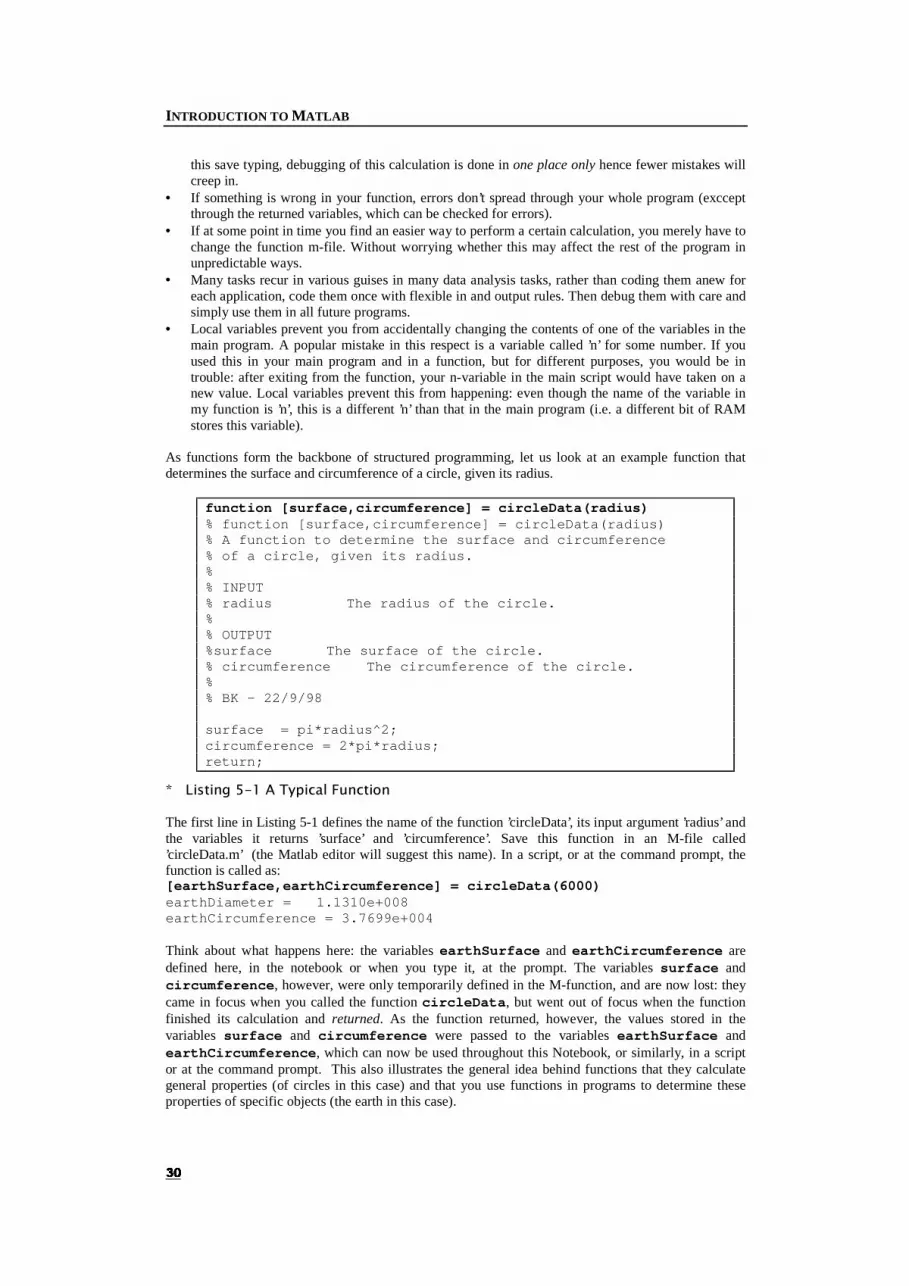
function [surface,circumference] = circleData(radius) % function [surface,circumference] = circleData(radius) % A function to determine the surface and circumference % of a circle, given its radius. % % INPUT % radius The radius of the circle. % % OUTPUT %surface The surface of the circle. % circumference The circumference of the circle. % % BK – 22/9/98 surface = pi*radius^2; circumference = 2*pi*radius; return;
� /LVWLQJ�����$�7\SLFDO�)XQFWLRQ�
The first line in Listing 5-1 defines the name of the function ’circleData’, its input argument ’radius’ and the variables it returns ’surface’ and ’circumference’. Save this function in an M-file called ’circleData.m’ (the Matlab editor will suggest this name). In a script, or at the command prompt, the function is called as: [earthSurface,earthCircumference] = circleData(6000) earthDiameter = 1.1310e+008 earthCircumference = 3.7699e+004 Think about what happens here: the variables earthSurface and earthCircumference are defined here, in the notebook or when you type it, at the prompt. The variables surface and circumference, however, were only temporarily defined in the M-function, and are now lost: they came in focus when you called the function circleData, but went out of focus when the function finished its calculation and returned. As the function returned, however, the values stored in the variables surface and circumference were passed to the variables earthSurface and earthCircumference, which can now be used throughout this Notebook, or similarly, in a script or at the command prompt. This also illustrates the general idea behind functions that they calculate general properties (of circles in this case) and that you use functions in programs to determine these properties of specific objects (the earth in this case).

CHAPTER 5: PROGRAMMING
� �
The function example also demonstrates a good coding habit. Start every M-file, script or function, with some explanatory comments. Comment lines start with the %-sign. Not only do these comments help you when you edit the file, they are also accessible to the Matlab help system. As an example, this is Matlab’s response to a request for help about circleData: help circleData function [surface,circumference] = circleData(radius) A function to determine the surface and circumference of a circle, given its radius. INPUT radius The radius of the circle. OUTPUT surface The surface of the circle. circumference The circumference of the circle. BK - 22/9/98 Matlab shows all comment lines in the M-file that form an uninterrupted block, starting from the first line. Note that for functions, the function definition itself (the first line) is not shown. That is why I repeat this line after a %-sign on the second line. This way, a call to help will quickly show me how to use this function: the order of the in- and output parameters, their meaning etc. This may seem somewhat superfluous when you first write the function, but you will start to forget these kind of things once you have set up a large library of your own data analysis functions. In normal use, you will probably write Matlab scripts and functions. The main script (program) could call other scripts. Variables defined in any of these scripts are available in all other scripts. In other words, the scope of the variables defined in one script includes other scripts. Some of the scripts will call functions to do small calculations that need only limited access to the data you are analysing. If a task or calculation relies on only a few variables and calculates only a few variables, a function is probably the best option. As soon as you are passing large numbers of arguments to the function, however, you may be better off doing the calculation in the main script. Or, for clarity, define another script to perform this task and call this script from the main script. It is good general programming practice to divide your program in as many scripts or functions as there are clearly identifiable separate tasks. In earlier versions of Matlab this sometimes led to a large number of M-files containing various scripts and functions. From Matlab 5, however, it is possible to define a function inside a function M-file. This makes your code easier to maintain and debug by separating out the tasks, but now without having to switch between large numbers of files to debug a single program. This does, however, add the decision level when to move a function to its own file. If a function defines a generally useful calculation, it will be called from other scripts than the current one and should therefore be placed in its own file. On the other hand, if the function defines some calculation that is unique to this function, you are probably better off defining it in the file in which it is used. This hides the function from other scripts (as well as from the help system). Part 2 of this book will discuss such design issues in more detail and explore them in real world applications. As mentioned above, each function creates its own workspace. Because variables are visible only to the workspace in which they are defined, functions have no access to the variables of the default workspace or the variables of another function. You should not look upon this as a restriction, but as a sensible feature. Hiding variables from parts of your application means that the parts run relatively independently and that they can be tested independently. This makes debugging much easier. Moreover, it allows you to reuse functions in many different applications. In very few instances you may want to circumvent this restricted visibility by defining variables as global. This is achieved by global A B

INTRODUCTION TO MATLAB
� �
defines the variables A and B as members of the global workspace. Note the absence of commas between the variables and the use of capitals. The latter is not compulsory, but a common way to distinguish local and global variables. If you want to access these variables in another workspace, for instance in a function, type global A B in that workspace, before accessing them. This tells the workspace that the value of the variable A should be looked up in the global workspace. Had you used A before declaring it as global, the function would assume that A is a variable of the local workspace and create it there, access to the global variable A would then be lost. This shows a clear disadvantage of the absence of data typing. To avoid such problems, put all global statements at the start of M-scripts and M-functions that require access to those variables. Global variables take up more storage space than local variables, and they can keep on using resources long after you stopped using them. Moreover, unless one is very careful declaring all relevant variables as global in all functions and scripts, considerable confusion can arise with some variables being global in one script and local in the other. Global variables are hardly ever necessary. When using functions, simply pass along the required variables as arguments. If you find you are passing long lists of variables to your functions, you have two options. First, if the calculations are only relevant to the application at hand, you can rewrite the functions as separate scripts. These scripts have access to all variables defined in the default workspace (the workspace of the command prompt and all scripts called from it). A second option is to use object oriented methods, roughly speaking this is a way to keep all the data that belong together, (for instance all the recorded spikes, analog data, equipment settings of a single experiment), together in a single object variable. Rather than passing all the individual bits of data to functions, you can pass the whole object for analysis inside the function. For details, see section The use of global variables is especially tempting when developing graphical user interfaces, where many small callback functions are defined to react to user input (such as button presses, keyboard input etc). Even there, global variables are not really needed, because data can be stored in the interface itself and collected when needed. GUIs developed this way are generally faster and easier to maintain. For details, see section 10.4.
���� )OH[LEOH�)XQFWLRQV�
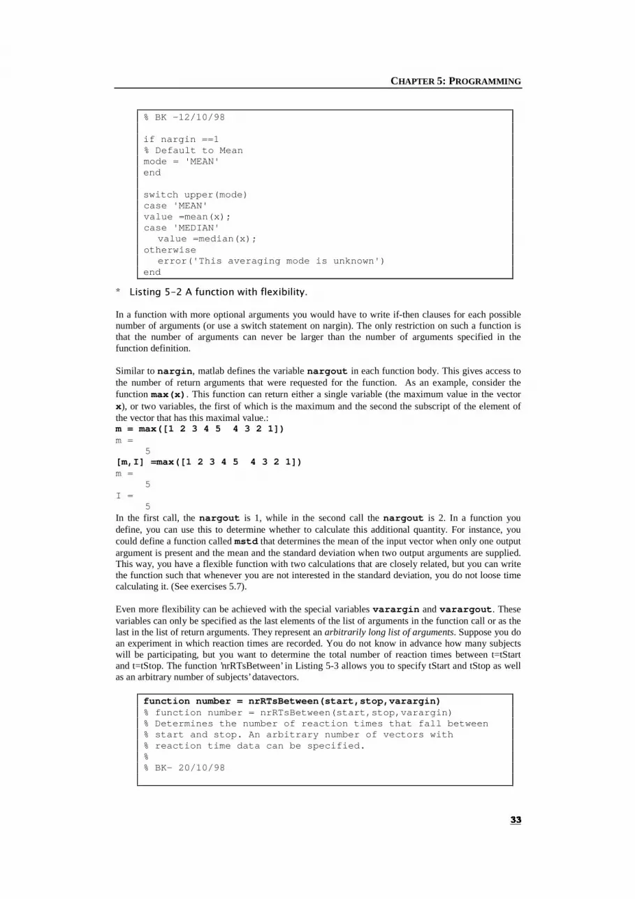
A structured program is a script that calls functions for common or repetitive tasks. The use of functions pays off most when you can reuse them in many applications. That implies, however, that functions should be flexible in the type of arguments that they receive, as there may be small differences in the way in which different programs will want to call a particular common function. Functions discussed up to here had a fixed number of arguments and returned a fixed number of variables. Functions can, however, be made more flexible. This is particularly useful in an objected oriented function that returns different objects depending on the context. This section explains how this is done. The simplest way to allow for some flexibility is to write the function body such that it can respond to different numbers of input and output arguments. Inside a function body, the variable nargin contains the number of input arguments. This is useful when some of the arguments of the function usually take on the same values, such default values could be coded into the function. Whenever the function is called without a value for these variables, the default values are used. In Listing 5-2, the function tests whether there is only a single argument, if so, the remaining second argument (the averaging mode) is defaulted to ’MEAN’.
function value = average(x,mode) % Determine the average of the data in x. The function % can use a median, mean or …. average depending on % the mode parameter % INPUT % x The vector of matrix with data. % [mode] The mode: median, mean. Defaults to % mean. % OUTPUT % value The average. %
CHAPTER 5: PROGRAMMING
� �
% BK –12/10/98 if nargin ==1 % Default to Mean mode = 'MEAN' end switch upper(mode) case 'MEAN' value =mean(x); case 'MEDIAN' value =median(x); otherwise error('This averaging mode is unknown') end
� /LVWLQJ�����$�IXQFWLRQ�ZLWK�IOH[LELOLW\��
In a function with more optional arguments you would have to write if-then clauses for each possible number of arguments (or use a switch statement on nargin). The only restriction on such a function is that the number of arguments can never be larger than the number of arguments specified in the function definition. Similar to nargin, matlab defines the variable nargout in each function body. This gives access to the number of return arguments that were requested for the function. As an example, consider the function max(x). This function can return either a single variable (the maximum value in the vector x), or two variables, the first of which is the maximum and the second the subscript of the element of the vector that has this maximal value.: m = max([1 2 3 4 5 4 3 2 1]) m = 5 [m,I] =max([1 2 3 4 5 4 3 2 1]) m = 5 I = 5 In the first call, the nargout is 1, while in the second call the nargout is 2. In a function you define, you can use this to determine whether to calculate this additional quantity. For instance, you could define a function called mstd that determines the mean of the input vector when only one output argument is present and the mean and the standard deviation when two output arguments are supplied. This way, you have a flexible function with two calculations that are closely related, but you can write the function such that whenever you are not interested in the standard deviation, you do not loose time calculating it. (See exercises 5.7). Even more flexibility can be achieved with the special variables varargin and varargout. These variables can only be specified as the last elements of the list of arguments in the function call or as the last in the list of return arguments. They represent an arbitrarily long list of arguments. Suppose you do an experiment in which reaction times are recorded. You do not know in advance how many subjects will be participating, but you want to determine the total number of reaction times between t=tStart and t=tStop. The function ’nrRTsBetween’ in Listing 5-3 allows you to specify tStart and tStop as well as an arbitrary number of subjects’ datavectors.
function number = nrRTsBetween(start,stop,varargin) % function number = nrRTsBetween(start,stop,varargin) % Determines the number of reaction times that fall between % start and stop. An arbitrary number of vectors with % reaction time data can be specified. % % BK- 20/10/98
INTRODUCTION TO MATLAB
� �
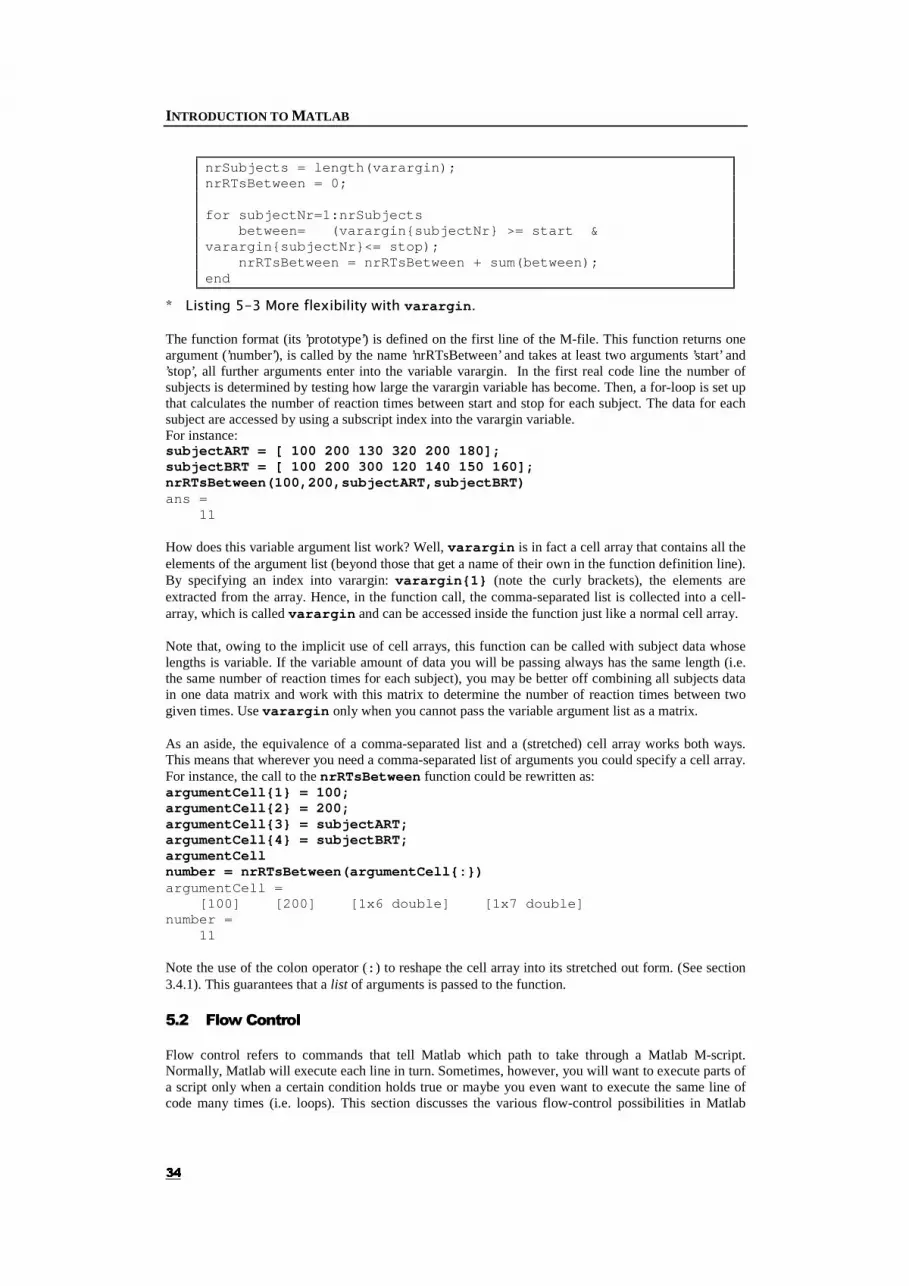
nrSubjects = length(varargin); nrRTsBetween = 0; for subjectNr=1:nrSubjects between= (varargin{subjectNr} >= start & varargin{subjectNr}<= stop); nrRTsBetween = nrRTsBetween + sum(between); end
� /LVWLQJ�����0RUH�IOH[LELOLW\�ZLWK�varargin��
The function format (its ’prototype’) is defined on the first line of the M-file. This function returns one argument (’number’), is called by the name ’nrRTsBetween’ and takes at least two arguments ’start’ and ’stop’, all further arguments enter into the variable varargin. In the first real code line the number of subjects is determined by testing how large the varargin variable has become. Then, a for-loop is set up that calculates the number of reaction times between start and stop for each subject. The data for each subject are accessed by using a subscript index into the varargin variable. For instance: subjectART = [ 100 200 130 320 200 180]; subjectBRT = [ 100 200 300 120 140 150 160]; nrRTsBetween(100,200,subjectART,subjectBRT) ans = 11 How does this variable argument list work? Well, varargin is in fact a cell array that contains all the elements of the argument list (beyond those that get a name of their own in the function definition line). By specifying an index into varargin: varargin{1} (note the curly brackets), the elements are extracted from the array. Hence, in the function call, the comma-separated list is collected into a cell-array, which is called varargin and can be accessed inside the function just like a normal cell array. Note that, owing to the implicit use of cell arrays, this function can be called with subject data whose lengths is variable. If the variable amount of data you will be passing always has the same length (i.e. the same number of reaction times for each subject), you may be better off combining all subjects data in one data matrix and work with this matrix to determine the number of reaction times between two given times. Use varargin only when you cannot pass the variable argument list as a matrix. As an aside, the equivalence of a comma-separated list and a (stretched) cell array works both ways. This means that wherever you need a comma-separated list of arguments you could specify a cell array. For instance, the call to the nrRTsBetween function could be rewritten as: argumentCell{1} = 100; argumentCell{2} = 200; argumentCell{3} = subjectART; argumentCell{4} = subjectBRT; argumentCell number = nrRTsBetween(argumentCell{:}) argumentCell = [100] [200] [1x6 double] [1x7 double] number = 11 Note the use of the colon operator (:) to reshape the cell array into its stretched out form. (See section 3.4.1). This guarantees that a list of arguments is passed to the function.
���� )ORZ�&RQWURO�
Flow control refers to commands that tell Matlab which path to take through a Matlab M-script. Normally, Matlab will execute each line in turn. Sometimes, however, you will want to execute parts of a script only when a certain condition holds true or maybe you even want to execute the same line of code many times (i.e. loops). This section discusses the various flow-control possibilities in Matlab
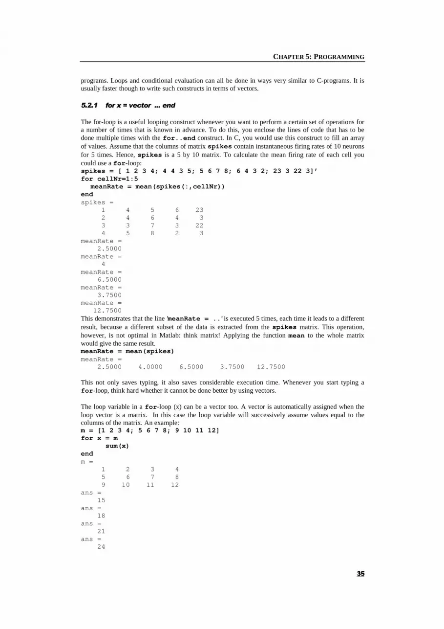
CHAPTER 5: PROGRAMMING
� �
programs. Loops and conditional evaluation can all be done in ways very similar to C-programs. It is usually faster though to write such constructs in terms of vectors. ������ IRU�[� �YHFWRU������HQG�
The for-loop is a useful looping construct whenever you want to perform a certain set of operations for a number of times that is known in advance. To do this, you enclose the lines of code that has to be done multiple times with the for..end construct. In C, you would use this construct to fill an array of values. Assume that the columns of matrix spikes contain instantaneous firing rates of 10 neurons for 5 times. Hence, spikes is a 5 by 10 matrix. To calculate the mean firing rate of each cell you could use a for-loop: spikes = [ 1 2 3 4; 4 4 3 5; 5 6 7 8; 6 4 3 2; 23 3 22 3]’ for cellNr=1:5 meanRate = mean(spikes(:,cellNr)) end spikes = 1 4 5 6 23 2 4 6 4 3 3 3 7 3 22 4 5 8 2 3 meanRate = 2.5000 meanRate = 4 meanRate = 6.5000 meanRate = 3.7500 meanRate = 12.7500 This demonstrates that the line ’meanRate = ..’ is executed 5 times, each time it leads to a different result, because a different subset of the data is extracted from the spikes matrix. This operation, however, is not optimal in Matlab: think matrix! Applying the function mean to the whole matrix would give the same result. meanRate = mean(spikes) meanRate = 2.5000 4.0000 6.5000 3.7500 12.7500 This not only saves typing, it also saves considerable execution time. Whenever you start typing a for-loop, think hard whether it cannot be done better by using vectors. The loop variable in a for-loop (x) can be a vector too. A vector is automatically assigned when the loop vector is a matrix. In this case the loop variable will successively assume values equal to the columns of the matrix. An example: m = [1 2 3 4; 5 6 7 8; 9 10 11 12] for x = m
sum(x) end m = 1 2 3 4 5 6 7 8 9 10 11 12 ans = 15 ans = 18 ans = 21 ans = 24
INTRODUCTION TO MATLAB
� �
But again, the same result in vector format can be obtained by exploiting Matlab’s matrix capabilities. sum(m) ans = 15 18 21 24 With experience in other programming languages, for-loops come to mind as the solution to every problem. In Matlab, however, they are rarely the optimal way to solve a problem. ������ ZKLOH�D�E�HQG�
The while loop is useful to perform a set of calculations a number of times, without knowing in advance how many iterations will be needed. The decision to continue the loop or to exit is taken after each iteration on the basis of the condition supplied after the while keyword. Let spikes be a vector containing the spike rates at certain times. spike(1) is the spikerate at time 1, spike(2) at time 2 etc. To determine the first time at which the spike rate drops below 10, a while-loop could be used:
spikes=[100 210 280 150 100 80 70 30 20 10 5 5 1 2 3]; time=1; while spikes(time)>=10 time=time+1; end belowThreshold = time belowThreshold = 11
What happens is that in line starting with ’while’, Matlab checks whether the element of the spikes vector at subscript time is larger than or equal to 10. If it is, the variable time is incremented after which Matlab jumps back to the start of the while-loop to check the next element of the spike vector. When the condition fails, the inside of the while-end loop is skipped and Matlab jumps to the line that sets the belowThreshold variable equal to the current value of the time variable. Note that here too, a vectorised approach is possible, and faster: belowThreshold = min(find(spikes<10)) belowThreshold = 11 In this code snippet I first use a logical operator to set all those entries of the spikes vector that have times below 10 to zero. Then the find function finds those values that are not zero (i.e. it returns those subscripts where the times are above or equal to 10). Finally, the min function returns the smallest of these subscripts. A while loop is often used to read text from files in conjunction with the fgets function. The fgets function returns –1 when the end of the file is found and a line of text in the file otherwise. You can use this to process all lines one by one. Assuming that fid is the file identifier of the file you want to read (see section 8.2 ) the loop would look something like: lineRead =1; while (lineRead ~= -1) lineRead = fgets(fid) %Do something with this line end This first initialises the variable lineRead to 1, to get the loop going. The while condition (lineRead ~=-1) evaluates to True hence the loop is executed. In the first line, a line is read from the file and this is stored in the lineRead variable. The something is done with this information after which execution goes back to the start of the while loop. Had the last call to fgets returned –1, which means that you have read all lines in the file and reached the end, the while condition would fail and the loop is exited. Hence this simple loop reads all the textlines in a file, regardless of how many lines there are.
CHAPTER 5: PROGRAMMING
� �
������ LI�D�E�HQG�
With the if-end and if-else-end constructs different bits of code can be executed in different circumstances. You could for instance decide on the basis of the number of spikes a cell fires to include it in an analysis or not. for cell = 1:5
if sum(spikes(:,cell)) > spikeThreshold %Do the analysis for this cell.
else disp([’Excluded cell ’ num2str(cell)] );
end end As an aside, the disp-command displays a text string. In this case the text string is a concatenation of two strings, the first is ’Excluded cell ’ , the second is the cell number that is converted from a number to a string by the function num2str. If-end constructs in combination with the break command can be used to exit for or while loops before they exit naturally. Consider the situation where you only want to analyse a specific number of cells (enoughCells). The following loop counts how many cells have been analysed and breaks the loop when enough cells have been done. When doneCells equals enoughCells, execution continues at the first line after the for-loop, without looping through the rest of the cells. doneCells =0; for cell = 1:nrCells
if sum(spikes(:,cell) > spikeThreshold %Do the analysis for this cell.
doneCells = doneCells +1; else
disp([’Excluded cell ’ num2str(cell)] ); end if (doneCells == enoughCells) break;
end end The if-break-end construct can also be used to break out of while-loops. ������ VZLWFK�FDVH�HQG�
Even though all conditional execution can in principle be done with combinations of if-then-else constructs, this can become quite opaque. Whenever you are programming many if-end constructs after another, consider using the switch-case-end construct. This will specifically be useful to process options to a command. Imagine for instance that you programmed a function that determines the central moment of a dataset that allows one to specify different kinds of central moments (’weighted’,’mean’,’median’). Assuming that the variable averagingMethod contains the selected method, a switch-statement to process these options would look like: switch lower(averagingMethod) case ’mean’ %Determine the arithmetic mean case ’median’ %Dermine the median
case ’weighted’ %Determine the weighted mean.
otherwise error([’This averaging method is unknown’ averagingMethod]); end The function lower is used to change the option string to all lower case letters. This provides an extra bit of flexibility, allowing the user of this function to use ’mean’ or ’Mean’ interchangeably. Whereas the
INTRODUCTION TO MATLAB
� �
case statements filter out those central-moment options that are known, the otherwise-statements catches those options that a user may supply, but have not been implemented. You could just ignore such options and wait for you program to produce unexpected results, but it is generally a good idea to try to catch all possible misuse of a function and respond to it with an error message that explains what is wrong. The error function displays the message (on the command prompt) and also terminates the program. This is discussed in more detail in the next section.
���� (UURU�+DQGOLQJ�
Matlab has a couple of functions that will help you to provide warnings to users whenever an unexpected situation arises. The first, disp , simply displays a string. A more sophisticated function is warning, which also displays a string, but this can be turned off or on globally with ’warning off’ and ’warning on’. This is useful when you write many warning messages in your code when you are developing a program but don’t want to see all of these messages when you start using the program "for real". To achieve this, simply type ’warning off’ before using the application. A further option, ’warning backtrace’ shows the warning string, but also displays a list of function calls that led to this warning. The function error not only displays an error message, it also passes control back to the command prompt. Use this whenever an error occurs from which the application cannot recover. Examples are a crucial argument that is missing in the function call, a variable containing a value that makes no sense, or a function is called with an option that has not been implemented. A recent addition to error handling in Matlab is the try-catch-end block. This construct allows you to try one set of commands and if these, for some reason, led to an error, perform another set. For instance try load filename catch warning([’Filename ’ filename ’ could not be opened’]); load matlab.mat end This code snippet will attempt to load the file whose filename is in the variable filename. If the load action fails for some reason (i.e. the file does not exist or cannot be opened), the file ’matlab.mat’ is opened instead. If this file cannot be loaded either, an error occurs. Note the use of a warning message inside the catch block. Without such a message you would never know that the file in filename could not be opened. Even though the try-catch construct is very useful to catch runtime errors that could not be foreseen when you were programming, it should be used with some care: trying one operation, catching the error and then trying another operation does take extra time to execute. If you know in advance that different arguments can be passed to a function and that in response to the type of argument a different calculation has to be performed, you should not use try-catch. Use if-then or switch-case instead.
���� 0LVFHOODQHRXV�3URJUDPPLQJ�7ULFNV�
This section discusses some techniques that have turned out to be useful in many Matlab applications, but do not fit in any of the other sections. ������ 3URJUDPPLQJ�ZLWK�HYDO�
The eval function takes a string argument and passes this to the Matlab command line. This means that the string is executed as if you typed it on the command line. Why is this useful? One example is when you loop through a whole dataset, say spike data of 10 neurons. You perform some kind of analysis on these and then want to save or print the results to file. You would need a different filename
CHAPTER 5: PROGRAMMING
� �
(based on the neurons’ name or id-number) for each analysis. Eval allows you to do this. Let’s assume that the datafiles are called ’neuron1.dat’ to ’neuron10.dat’ and you want to store the results of the analysis (say a figure) as an encapsulated postscript file called neuronXAnalysis.eps where X is the number of the neuron. This kind of batch processing can only be done with eval:
for neuronNr = 1:10 % Create the load command. loadString = [’load neuron’ num2str(neuronNR) ’.dat’]; % Execute the load command. eval(loadString) % Do the analysis here. Assume this generates a figure % with the calculated properties. % Create the print command to print the current figure. printString = [’print -deps neuron’ num2str(neuronNr) ’Analysis.exp’]; % Execute the print command. eval(printString); end
� /LVWLQJ�����$Q�H[DPSOH�RI�XVLQJ�HYDO��
When using eval, be sure to setup the string to be executed in a separate variable and, in the debugging phase, check its value before execution. Errors creep in easily! See exercise 4 in chapter 6, for a working demonstration of eval.
���� 8VLQJ�ODUJH�DUUD\V�
When you need to use large matrices, always try to initialise them before you put data into them with the zeros commands. For instance: m= zeros(100,100) initialises a 100*100 matrix with all its entries set to zero. After this initialisation you can proceed to read the actual data into the matrix one-by-one (or whichever way you like). A speed increase is gained here because Matlab needs to allocate memory for this variable only once. If instead, you read data from file and extended the matrix on the fly, the memory reserved for this matrix would have to be reallocated many times anew and this costs time. Strictly, this method only works if you know before filling the matrix how large it will be. If this is not the case, it may be worthwhile to block your memory allocations. This means that you would allocate a large matrix to start with (say 100*100) , fill these values and when you reach the point that the matrix is full, allocate another large block. Keep on doing this until all entries have been filled with their correct values. Then chechk whether you have allocated any elements in the matrix which weren’t necessary after all. Remove these by setting them equal to the empty matrix. If you use very large matrices whose entries are almost all zero, it is worthwhile to delve into sparse matrices. These matrices represent their contents in a different way than normal matrices. I.e. they assume that an entry is zero unless it is explicitly represented to be something else. Clearly, if you have a 1000*1000 matrix in which only the diagonal entries are non-zero, this saves a lot of storage space. In this case 1000*1000*8bytes ~ 8Mbytes whereas the diagonal elements need only 100*8 ~ 800 bytes. Although the internal representation of these matrices is different, they can be used just as any other matrices (i.e. for multiplication, addition etc).
���� )XUWKHU�5HDGLQJ�
Programming in Matlab is the subject of chapter 10 in the Matlab User’s guide. Apart from the subjects covered above, it discusses techniques to optimize your code, to obtain user input from the command line and many other things. Read it. To gain more experience with programming, spend a lot of time on the exercises as well as the projects in part 2 of this book. You can only learn this by trying and doing it yourself!
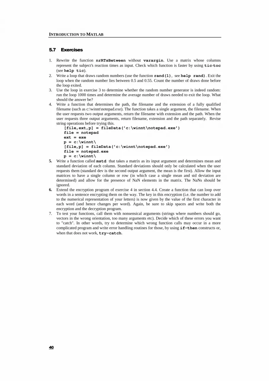
INTRODUCTION TO MATLAB
� �
���� ([HUFLVHV�
1. Rewrite the function nrRTsBetween without varargin. Use a matrix whose columns represent the subject’s reaction times as input. Check which function is faster by using tic-toc (see help tic).
2. Write a loop that draws random numbers (use the function rand(1), see help rand). Exit the loop when the random number lies between 0.5 and 0.55. Count the number of draws done before the loop exited.
3. Use the loop in exercise 3 to determine whether the random number generator is indeed random: run the loop 1000 times and determine the average number of draws needed to exit the loop. What should the answer be?
4. Write a function that determines the path, the filename and the extension of a fully qualified filename (such as c:\winnt\notepad.exe). The function takes a single argument, the filename. When the user requests two output arguments, return the filename with extension and the path. When the user requests three output arguments, return filename, extension and the path separately. Revise string operations before trying this.
[file,ext,p] = fileData(’c:\winnt\notepad.exe’) file = notepad ext = exe p = c:\winnt\ [file,p] = fileData(’c:\winnt\notepad.exe’) file = notepad.exe p = c:\winnt\
5. Write a function called mstd that takes a matrix as its input argument and determines mean and standard deviation of each column. Standard deviations should only be calculated when the user requests them (standard dev is the second output argument, the mean is the first). Allow the input matrices to have a single column or row (in which case a single mean and std deviation are determined) and allow for the presence of NaN elements in the matrix. The NaNs should be ignored.
6. Extend the encryption program of exercise 4 in section 4.4. Create a function that can loop over words in a sentence encrypting them on the way. The key in this encryption (i.e. the number to add to the numerical representation of your letters) is now given by the value of the first character in each word (and hence changes per word). Again, be sure to skip spaces and write both the encryption and the decryption program.
7. To test your functions, call them with nonsensical arguments (strings where numbers should go, vectors in the wrong orientation, too many arguments etc). Decide which of these errors you want to "catch". In other words, try to determine which wrong function calls may occur in a more complicated program and write error handling routines for those, by using if-then constructs or, when that does not work, try-catch.
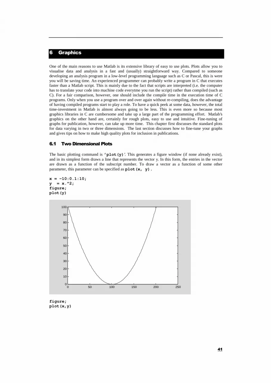
� �
�� *UDSKLFV�
One of the main reasons to use Matlab is its extensive library of easy to use plots. Plots allow you to visualise data and analysis in a fast and (usually) straightforward way. Compared to someone developing an analysis program in a low-level programming language such as C or Pascal, this is were you will be saving time. An experienced programmer can probably write a program in C that executes faster than a Matlab script. This is mainly due to the fact that scripts are interpreted (i.e. the computer has to translate your code into machine code everytme you run the script) rather than compiled (such as C). For a fair comparison, however, one should include the compile time in the execution time of C programs. Only when you use a program over and over again without re-compiling, does the advantage of having compiled programs start to play a role. To have a quick peek at some data, however, the total time-investment in Matlab is almost always going to be less. This is even more so because most graphics libraries in C are cumbersome and take up a large part of the programming effort. Matlab’s graphics on the other hand are, certainly for rough plots, easy to use and intuitive. Fine-tuning of graphs for publication, however, can take up more time. This chapter first discusses the standard plots for data varying in two or three dimensions. The last section discusses how to fine-tune your graphs and gives tips on how to make high quality plots for inclusion in publications.
���� 7ZR�'LPHQVLRQDO�3ORWV�
The basic plotting command is ’plot(y)’. This generates a figure window (if none already exist), and in its simplest form draws a line that represents the vector y. In this form, the entries in the vector are drawn as a function of the subscript number. To draw a vector as a function of some other parameter, this parameter can be specified as plot(x, y). x = -10:0.1:10; y = x.^2; figure; plot(y)
0 50 100 150 200 2500
10
20
30
40
50
60
70
80
90
100
figure; plot(x,y)

INTRODUCTION TO MATLAB
� �
-10 -8 -6 -4 -2 0 2 4 6 8 100
10
20
30
40
50
60
70
80
90
100
Here I opened a new figure window by issuing the figure command. To add a second line to the same figure, first ’hold’ the current figure, then issue another plot command: plot(x,y) hold on plot(x,y+25)
-10 -8 -6 -4 -2 0 2 4 6 8 100
20
40
60
80
100
120
140
Two lines in the same linestyle can become confusing, Matlab allows you to specify different styles for the lines you plot. This is achieved by adding a string to the plot call. This string also specifies the colour of the line: clf; %Clear the figure plot(x,y,’r:’) %Plot a dotted line in red hold on plot(x,y+25,’y-.’) %Add a dashed-dotted line in yellow.

CHAPTER 6: GRAPHICS
� �
-10 -8 -6 -4 -2 0 2 4 6 8 100
20
40
60
80
100
120
140
A complete list of line options can be found under help plot. The default plot command connects the dataopoints in the vectors x,y by linearly interpolating lines. This is not always desirable. The third argument to the plot function can be used to plot only the datapoints: x=0:5:25; y = x.^2; clf; plot(x,y,’+r’) %Plot the datapoints with red ’+’ markers . hold on plot(x,2*y,’*y’) %Plot these datapoints with yellow ’*’ markers.
0 5 10 15 20 250
200
400
600
800
1000
1200
1400
You can create a plot showing both lines and datapoint markers by using the hold function, but it is more easily done by doubling the call to the plot function: clf; plot(x,y,’+r’,x,y,’:r’) % Plot red ’+’ datamarkers and connect them
% with a red dotted line.
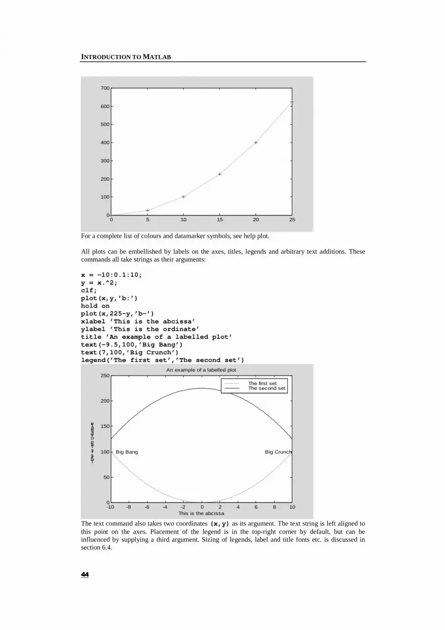
INTRODUCTION TO MATLAB
� �
0 5 10 15 20 250
100
200
300
400
500
600
700
For a complete list of colours and datamarker symbols, see help plot. All plots can be embellished by labels on the axes, titles, legends and arbitrary text additions. These commands all take strings as their arguments: x = -10:0.1:10; y = x.^2; clf; plot(x,y,’b:’) hold on plot(x,225-y,’b-’) xlabel ’This is the abcissa’ ylabel ’This is the ordinate’ title ’An example of a labelled plot’ text(-9.5,100,’Big Bang’) text(7,100,’Big Crunch’) legend(’The first set’,’The second set’)
-10 -8 -6 -4 -2 0 2 4 6 8 100
50
100
150
200
250
This is the abcissa
This is the ordinate
An example of a labelled plot
Big Bang Big Crunch
The first setThe second set
The text command also takes two coordinates (x,y) as its argument. The text string is left aligned to this point on the axes. Placement of the legend is in the top-right corner by default, but can be influenced by supplying a third argument. Sizing of legends, label and title fonts etc. is discussed in section 6.4.
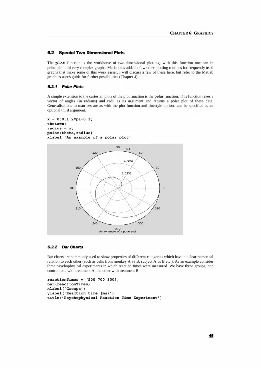
CHAPTER 6: GRAPHICS
� �
���� 6SHFLDO�7ZR�'LPHQVLRQDO�3ORWV�
The plot function is the workhorse of two-dimensional plotting, with this function one can in principle build very complex graphs. Matlab has added a few other plotting routines for frequently used graphs that make some of this work easier. I will discuss a few of these here, but refer to the Matlab graphics user’s guide for further possibilities (Chapter 4). ������ 3RODU�3ORWV�
A simple extension to the cartesian plots of the plot function is the polar function. This function takes a vector of angles (in radians) and radii as its argument and returns a polar plot of these data. Generalisations to matrices are as with the plot function and linestyle options can be specified as an optional third argument. x = 0:0.1:2*pi-0.1; theta=x; radius = x; polar(theta,radius) xlabel ’An example of a polar plot’
An example of a polar plot
2.0333
4.0667
6.1
30
210
60
240
90
270
120
300
150
330
180 0
������ %DU�&KDUWV���
Bar charts are commonly used to show properties of different categories which have no clear numerical relation to each other (such as cells from monkey A vs B, subject A vs B etc.). As an example consider three psychophysical experiments in which reaction times were measured. We have three groups, one control, one with treatment A, the other with treatment B. reactionTimes = [500 700 300]; bar(reactionTimes) xlabel(’Groups’) ylabel(’Reaction time (ms)’) title(’Psychophysical Reaction Time Experiment’)

INTRODUCTION TO MATLAB
� �
1 2 30
100
200
300
400
500
600
700
Groups
Reaction time (ms)
Psychophysical Reaction Time Experiment
Suppose however that you want to display the data of the individual subjects in each of the groups. In that case, your data will form a matrix: individualReactionTimes = [500 450 550; 675 700 725; 200 300 400]; bar(individualReactionTimes) ; xlabel(’Groups’) ylabel(’Reaction time (ms)’) title(’Psychophysical Reaction Time Experiment’)
1 2 30
100
200
300
400
500
600
700
800
Groups
Reaction time (ms)
Psychophysical Reaction Time Experiment
Hence, each row in the matrix is shown as a group, and each element of a row is a single bar showing a reaction time of a single subject. The details of how to display these charts as horizontal barcharts, 3D bar charts or stacked bar charts can be found in the graphics manual.
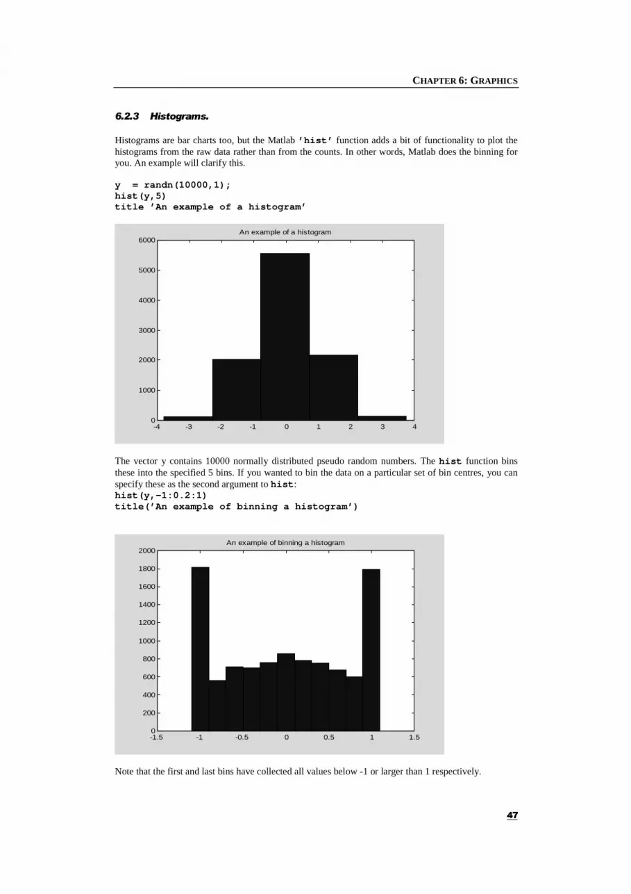
CHAPTER 6: GRAPHICS
� �
������ +LVWRJUDPV��
Histograms are bar charts too, but the Matlab ’hist’ function adds a bit of functionality to plot the histograms from the raw data rather than from the counts. In other words, Matlab does the binning for you. An example will clarify this. y = randn(10000,1); hist(y,5) title ’An example of a histogram’
-4 -3 -2 -1 0 1 2 3 40
1000
2000
3000
4000
5000
6000An example of a histogram
The vector y contains 10000 normally distributed pseudo random numbers. The hist function bins these into the specified 5 bins. If you wanted to bin the data on a particular set of bin centres, you can specify these as the second argument to hist: hist(y,-1:0.2:1) title(’An example of binning a histogram’)
-1.5 -1 -0.5 0 0.5 1 1.50
200
400
600
800
1000
1200
1400
1600
1800
2000An example of binning a histogram
Note that the first and last bins have collected all values below -1 or larger than 1 respectively.
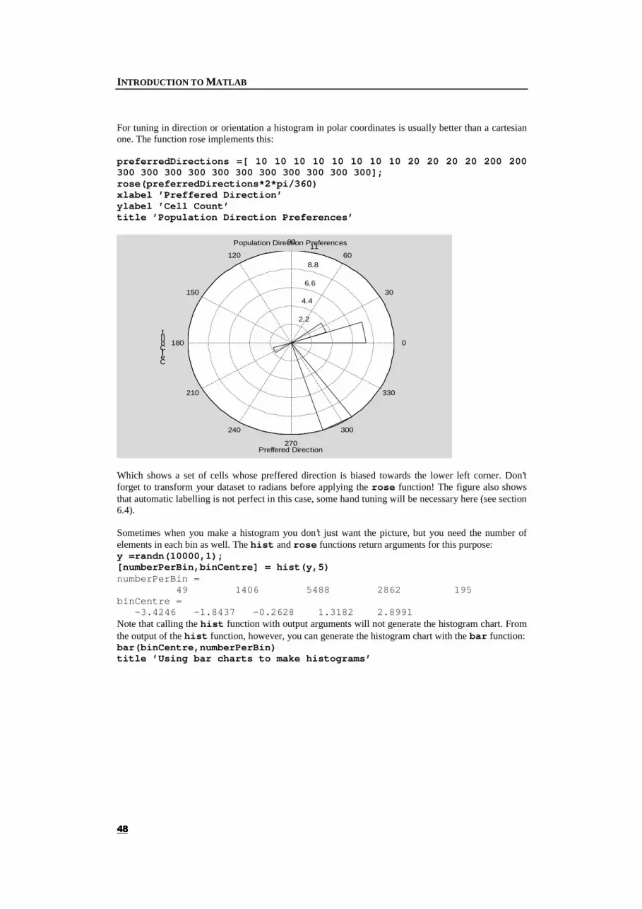
INTRODUCTION TO MATLAB
� �
For tuning in direction or orientation a histogram in polar coordinates is usually better than a cartesian one. The function rose implements this: preferredDirections =[ 10 10 10 10 10 10 10 10 20 20 20 20 200 200 300 300 300 300 300 300 300 300 300 300 300]; rose(preferredDirections*2*pi/360) xlabel ’Preffered Direction’ ylabel ’Cell Count’ title ’Population Direction Preferences’
Preffered Direction
Cell Count
Population Direction Preferences
2.2
4.4
6.6
8.8
11
30
210
60
240
90
270
120
300
150
330
180 0
Which shows a set of cells whose preffered direction is biased towards the lower left corner. Don’t forget to transform your dataset to radians before applying the rose function! The figure also shows that automatic labelling is not perfect in this case, some hand tuning will be necessary here (see section 6.4). Sometimes when you make a histogram you don’t just want the picture, but you need the number of elements in each bin as well. The hist and rose functions return arguments for this purpose: y =randn(10000,1); [numberPerBin,binCentre] = hist(y,5) numberPerBin = 49 1406 5488 2862 195 binCentre = -3.4246 -1.8437 -0.2628 1.3182 2.8991 Note that calling the hist function with output arguments will not generate the histogram chart. From the output of the hist function, however, you can generate the histogram chart with the bar function: bar(binCentre,numberPerBin) title ’Using bar charts to make histograms’

CHAPTER 6: GRAPHICS
� �
-5 -4 -3 -2 -1 0 1 2 3 40
1000
2000
3000
4000
5000
6000Using bar charts to make histograms
The function rose also returns bincentres and numbers per bin, but to plot these data on a polar grid, you will have to use the polar function. ������ $UURZ�3ORWV��&RPSDVV��)HDWKHU��4XLYHU��
Directions, velocities and orientations are most easily depicted with arrows. Matlab provides the compass function which plots arrows emanating from the origin of a polar coordinate system, the feather function which shows arrows emanating from a horizontal line and the quiver function with which you can plot arros at arbitrary positions in two or even three dimensional space. Strangely, all these functions require cartesian coordinates as input. To make their use somewhat easier, use the functions that convert between polar and cartesian coordinates: pol2cart and cart2pol. As an example, consider the population of direction tuned neurons discussed in the example of the rose plot above. Suppose that apart from their preferred directions, we also know the firing rate of these neurons when stimulated in their preferred direction. preferredDirections =[ 10 10 10 10 10 10 10 10 20 20 20 20 200 200 300 300 300 300 300 300 300 300 300 300 300]; firingRate = [100 110 120 200 100 120 130 123 60 70 50 50 100 150 230 250 250 240 250 230 234 260 290 290 290 ]; [cartDirections,cartRates] = pol2cart(preferredDirections*2*pi/360,firingRate); compass(cartDirections,cartRates); xlabel ’A Compass Plot’
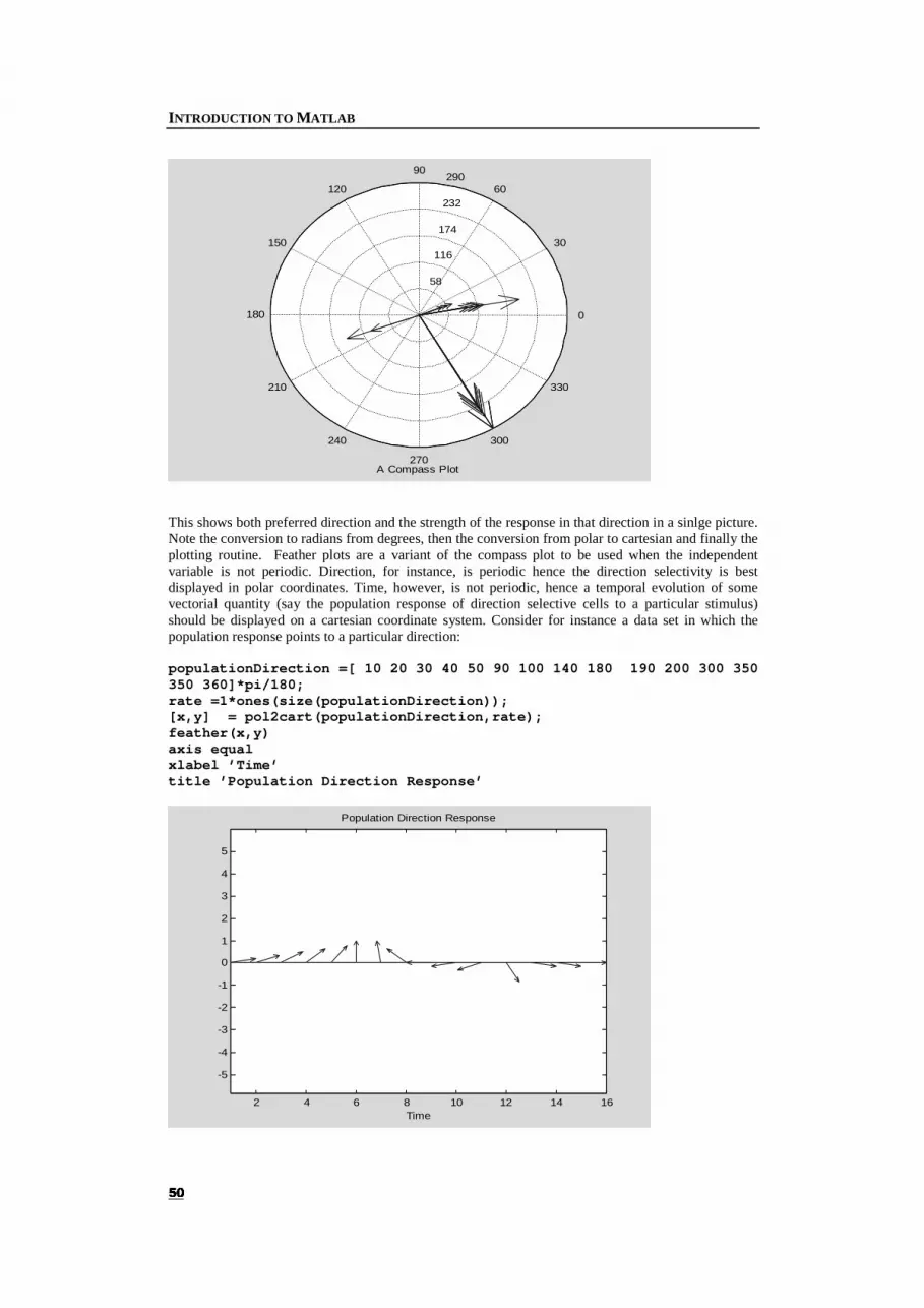
INTRODUCTION TO MATLAB
� �
A Compass Plot
58
116
174
232
290
30
210
60
240
90
270
120
300
150
330
180 0
This shows both preferred direction and the strength of the response in that direction in a sinlge picture. Note the conversion to radians from degrees, then the conversion from polar to cartesian and finally the plotting routine. Feather plots are a variant of the compass plot to be used when the independent variable is not periodic. Direction, for instance, is periodic hence the direction selectivity is best displayed in polar coordinates. Time, however, is not periodic, hence a temporal evolution of some vectorial quantity (say the population response of direction selective cells to a particular stimulus) should be displayed on a cartesian coordinate system. Consider for instance a data set in which the population response points to a particular direction: populationDirection =[ 10 20 30 40 50 90 100 140 180 190 200 300 350 350 360]*pi/180; rate =1*ones(size(populationDirection)); [x,y] = pol2cart(populationDirection,rate); feather(x,y) axis equal xlabel ’Time’ title ’Population Direction Response’
2 4 6 8 10 12 14 16
-5
-4
-3
-2
-1
0
1
2
3
4
5
Time
Population Direction Response

CHAPTER 6: GRAPHICS
� �
Quiver plots, finally, give complete freedom to place arrows in the plotting area. A two-dimensional quiver, for instance, takes for arguments. The first two specify the x,y location of the base of the arrow, while the next two u,v specify the direction of the arrow. A fifth argument can be used to scale the arrows. The quiver function is clearly very useful to display optic flow or other vector fields. The graphics manual shows an example of how this can be used to clarify the structure of a complicated surface by adding arrows that represent the gradients of the surface.
���� 7KUHH�'LPHQVLRQDO�3ORWV�
The straightforward generalisation of the plot function is the plot3 function which takes x,y as well as z vector or matrix arguments. Each point in these vectors is plotted as a point in the graph and interpolating lines can connect these datapoints. Multiple lines can be plotted by specifying matrix arguments for X, Y, Z, where each column corresponds to a single line. The plot3 function draws lines in three-dimensional space. To visualise matrices that represent depedencies of data on two independent variables rather than vectors, which were discussed in the previous section, Matlab provides the functions surf and mesh. To illustrate this, I use the function peaks which is just a matrix that looks nice. mesh(peaks) xlabel ’X-axis’ ylabel ’Y-axis’ zlabel ’Z-axis’ title ’The Peaks Function’
surf(peaks) xlabel ’X-axis’ ylabel ’Y-axis’ zlabel ’Z-axis’ title ’The Peaks Function’
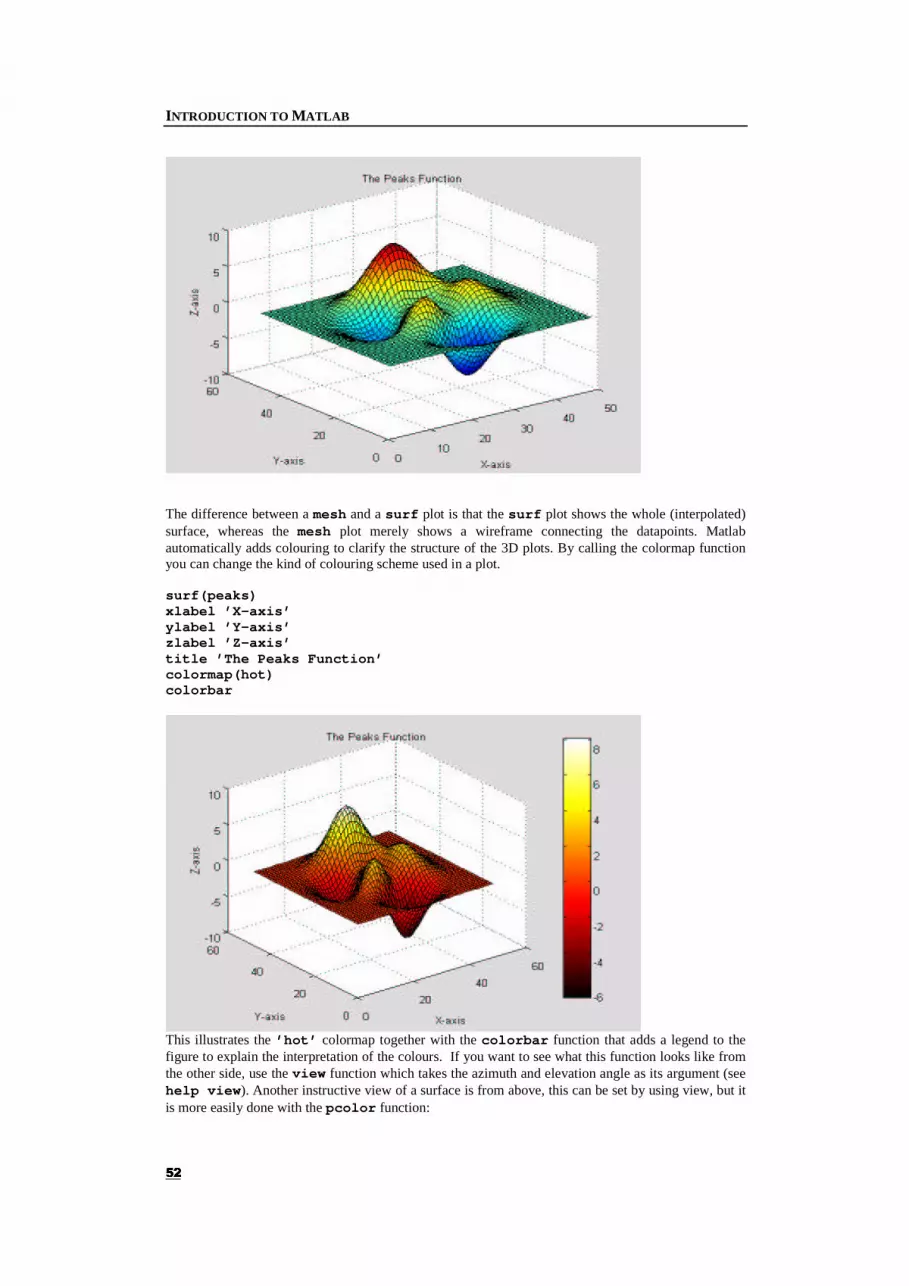
INTRODUCTION TO MATLAB
� �
The difference between a mesh and a surf plot is that the surf plot shows the whole (interpolated) surface, whereas the mesh plot merely shows a wireframe connecting the datapoints. Matlab automatically adds colouring to clarify the structure of the 3D plots. By calling the colormap function you can change the kind of colouring scheme used in a plot. surf(peaks) xlabel ’X-axis’ ylabel ’Y-axis’ zlabel ’Z-axis’ title ’The Peaks Function’ colormap(hot) colorbar
This illustrates the ’hot’ colormap together with the colorbar function that adds a legend to the figure to explain the interpretation of the colours. If you want to see what this function looks like from the other side, use the view function which takes the azimuth and elevation angle as its argument (see help view). Another instructive view of a surface is from above, this can be set by using view, but it is more easily done with the pcolor function:
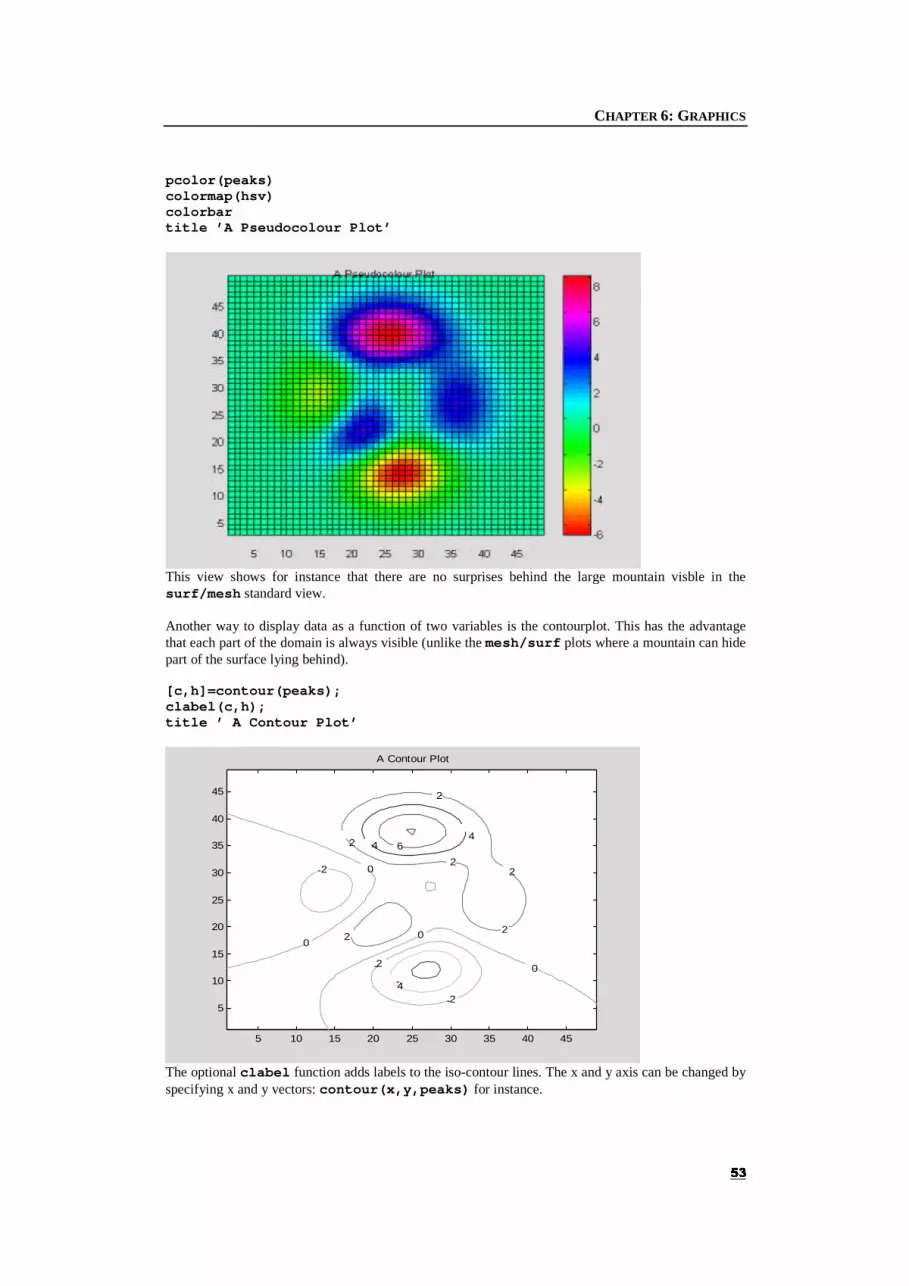
CHAPTER 6: GRAPHICS
� �
pcolor(peaks) colormap(hsv) colorbar title ’A Pseudocolour Plot’
This view shows for instance that there are no surprises behind the large mountain visble in the surf/mesh standard view. Another way to display data as a function of two variables is the contourplot. This has the advantage that each part of the domain is always visible (unlike the mesh/surf plots where a mountain can hide part of the surface lying behind). [c,h]=contour(peaks); clabel(c,h); title ’ A Contour Plot’
5 10 15 20 25 30 35 40 45
5
10
15
20
25
30
35
40
45
A Contour Plot
-4
-2
-2
-2
0
0
0
0 2
2
2
2
2
2
4 4 6
The optional clabel function adds labels to the iso-contour lines. The x and y axis can be changed by specifying x and y vectors: contour(x,y,peaks) for instance.

INTRODUCTION TO MATLAB
� �
To display data that vary as a function of more than one variable, three-dimensional plots must be used. It can be quite a lot of work to get these three dimensional pictures to look "just right". This is not some shortcoming of Matlab but rather the fact that paper and your computer screen are two-dimensional. This means that you will have to choose a point of view from which to look at the whole three-dimensional structure. If you take the wrong point of view, the interesting structure in your data may remain hidden. Drawings can be much improved by using lighting, shading, colouring, adding or removing grids, judicious labelling, the combination of contour with surface plots or even an occasional quiver plot on top of a surface. All of this requires a lot of experimentation and patience. Before you start developing more complicated plots, browse through the graphics manual to see whether there is no other way to plot the same data or maybe a predefined Matlab function that does just what you want. It is also worth considering before you start whether a coloured drawing will be acceptable for a publication, otherwise it may be a waste of time. Also, Matlab 3D plots are turned into bitmaps when exported, this can have nasty consequences when you try to import them into other packages such as Word or Powerpoint. Unlike one-dimensional plots, they are not easy to edit! See also section 6.5.
���� )LQH�7XQLQJ�
Figures can be enhanced by the use of subplot which allow you to display multiple subplots in a single figure. The command subplot(2,31) for instance, generates a figure with 2 rows with 3 axes each and it makes the first axis the current one. I.e. all plotting commands will be directed towards the first subplot. subplot(2,3,1) plot(1:10,(1:10).^2,’:b’) subplot(2,3,2) plot(1:10,10 - (1:10).^2,’-.b’) subplot(2,3,6) plot(1:10,sin (1:10).^2,’-b’) title ’An example of using subplots’
0 5 100
20
40
60
80
100
0 5 10-100
-50
0
50
0 5 100
0.2
0.4
0.6
0.8
1An example of using subplots
Labels and legends can be added to subplots by calling these functions when that particular axis is current. The current axis is the one referred to by the last call to the subplot function. What is really going on in the subplot function is that Matlab generates more than one set of axes. The subplot function always does this in a "rectangular" form. I.e.it does not allow you to generate three subplots. To do this you will have to use the axes function which creates an additional set of axes in the current figure at the specified position. figure; axes(’position’,[0.07 0.1 0.4 0.8]);
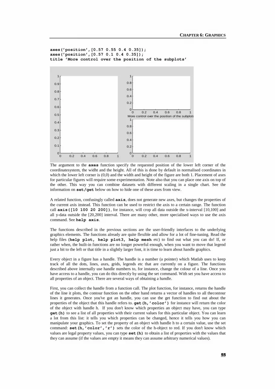
CHAPTER 6: GRAPHICS
� �
axes(’position’,[0.57 0.55 0.4 0.35]); axes(’position’,[0.57 0.1 0.4 0.35]); title ’More control over the position of the subplots’
0 0.2 0.4 0.6 0.8 10
0.1
0.2
0.3
0.4
0.5
0.6
0.7
0.8
0.9
1
0 0.2 0.4 0.6 0.8 10
0.2
0.4
0.6
0.8
1
0 0.2 0.4 0.6 0.8 10
0.2
0.4
0.6
0.8
1More control over the position of the subplots
The argument to the axes function specify the requested position of the lower left corner of the coordinatesystem, the widht and the height. All of this is done by default in normalised coordinates in which the lower left corner is (0,0) and the width and height of the figure are both 1. Placement of axes for particular figures will require some experimentation. Note also that you can place one axis on top of the other. This way you can combine datasets with different scaling in a single chart. See the information on set/get below on how to hide one of these axes from view. A related function, confusingly called axis, does not generate new axes, but changes the properties of the current axis instead. This function can be used to restrict the axis to a certain range. The function call axis([10 100 20 200]), for instance, will crop all data outside the x-interval [10,100] and all y-data outside the [20,200] interval. There are many other, more specialised ways to use the axis command. See help axis. The functions described in the previous sections are the user-friendly interfaces to the underlying graphics elements. The functions already are quite flexible and allow for a lot of fine-tuning. Read the help files (help plot, help plot3, help mesh etc) to find out what you can do! If, or rather when, the built-in functions are no longer powerful enough, when you want to move that legend just a bit to the left or that title in a slightly larger font, it is time to learn about handle graphics. Every object in a figure has a handle. The handle is a number (a pointer) which Matlab uses to keep track of all the dots, lines, axes, grids, legends etc that are currently on a figure. The functions described above internally use handle numbers to, for instance, change the colour of a line. Once you have access to a handle, you can do this directly by using the set command. With set you have access to all properties of an object. There are several ways of obtaining a handle. First, you can collect the handle from a function call. The plot function, for instance, returns the handle of the line it plots, the contour function on the other hand returns a vector of handles to all thecontour lines it generates. Once you’ve got an handle, you can use the get function to find out about the properties of the object that this handle refers to. get(h,’color’) for instance will return the color of the object with handle h. If you don’t know which properties an object may have, you can type get(h) to see a list of all properties with their current values for this particular object. You can learn a lot from this list: it tells you which properties can be changed, hence it tells you how you can manipulate your graphics. To set the property of an object with handle h to a certain value, use the set command: set(h,’color’,’r’) sets the color of the h-object to red. If you don’t know which values are legal property values, you can type set(h) to obtain a list of properties with the values that they can assume (if the values are empty it means they can assume arbitrary numerical values).

INTRODUCTION TO MATLAB
� �
figure; x = -10:0.1:10; y = x.^2; lineHandle = plot(x,y,’r-’) lineHandle = 3.0002
-10 -8 -6 -4 -2 0 2 4 6 8 100
10
20
30
40
50
60
70
80
90
100
This example shows that the red line in the above figure has the handle 1.0011. To find out about the properties of this line use the get and set command. Left in the table are the current properties of this line, obtained with get and on the right the legal property values obtained with set.
get(lineHandle)
Color = [1 0 0] EraseMode = normal LineStyle = - LineWidth = [0.5] Marker = none MarkerSize = [6] MarkerEdgeColor = auto MarkerFaceColor = none XData = [ (1 by 201) double array] YData = [ (1 by 201) double array] ZData = [] ButtonDownFcn = Children = [] Clipping = on CreateFcn = DeleteFcn = BusyAction = queue HandleVisibility = on HitTest = on Interruptible = on Parent = [2.00012] Selected = off SelectionHighlight = on Tag = Type = line UIContextMenu = [] UserData = [] Visible = on
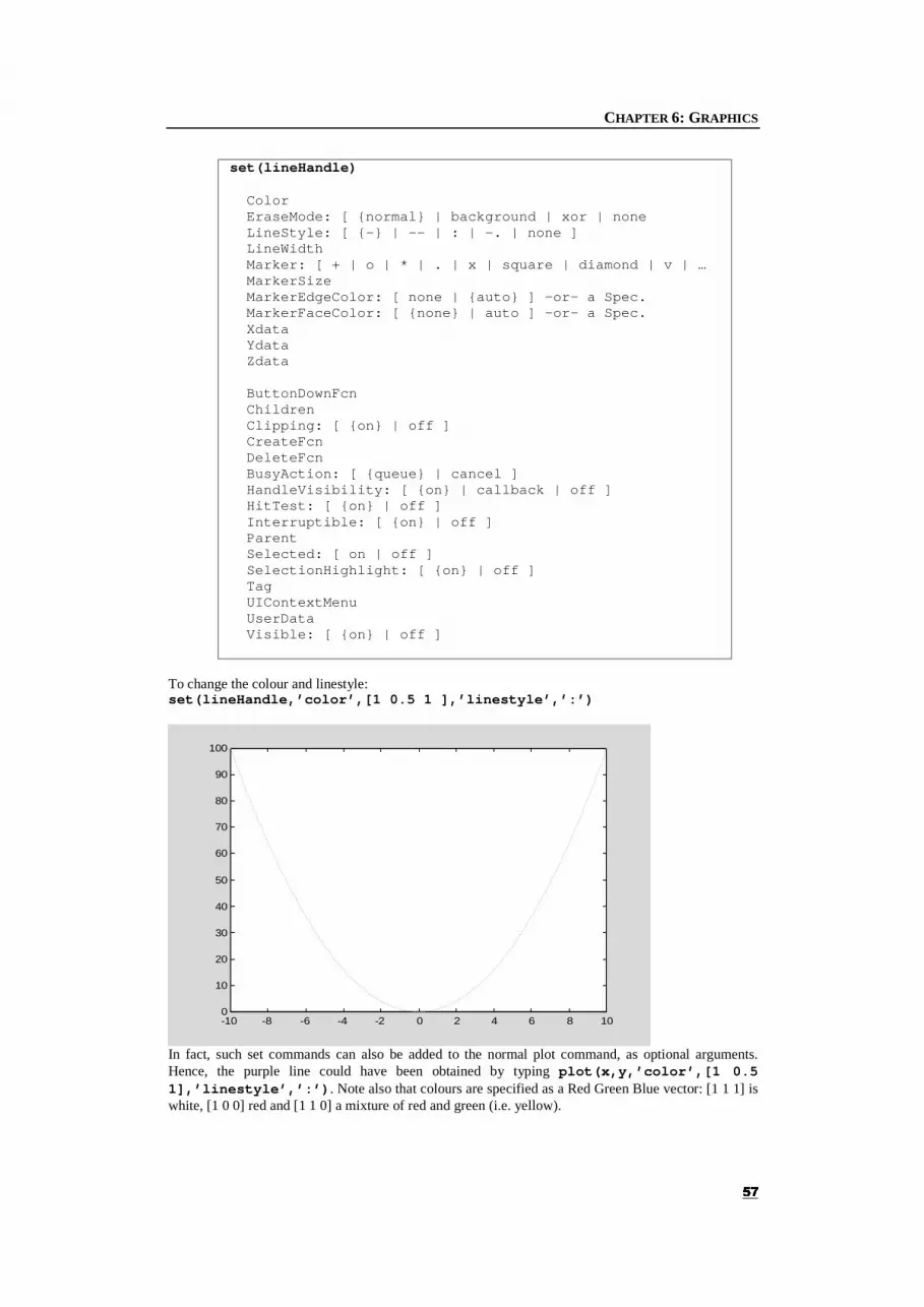
CHAPTER 6: GRAPHICS
� �
set(lineHandle) Color EraseMode: [ {normal} | background | xor | none LineStyle: [ {-} | -- | : | -. | none ] LineWidth Marker: [ + | o | * | . | x | square | diamond | v | … MarkerSize MarkerEdgeColor: [ none | {auto} ] -or- a Spec. MarkerFaceColor: [ {none} | auto ] -or- a Spec. Xdata Ydata Zdata ButtonDownFcn Children Clipping: [ {on} | off ] CreateFcn DeleteFcn BusyAction: [ {queue} | cancel ] HandleVisibility: [ {on} | callback | off ] HitTest: [ {on} | off ] Interruptible: [ {on} | off ] Parent Selected: [ on | off ] SelectionHighlight: [ {on} | off ] Tag UIContextMenu UserData Visible: [ {on} | off ]
To change the colour and linestyle: set(lineHandle,’color’,[1 0.5 1 ],’linestyle’,’:’)
-10 -8 -6 -4 -2 0 2 4 6 8 100
10
20
30
40
50
60
70
80
90
100
In fact, such set commands can also be added to the normal plot command, as optional arguments. Hence, the purple line could have been obtained by typing plot(x,y,’color’,[1 0.5 1],’linestyle’,’:’). Note also that colours are specified as a Red Green Blue vector: [1 1 1] is white, [1 0 0] red and [1 1 0] a mixture of red and green (i.e. yellow).
INTRODUCTION TO MATLAB
� �
As mentioned before, every object on the figure (and even the figure itself) has a handle. The handles can be obtained when the object is created, as used in the plot example above. This uses the feature that most plotting functions return the handles of the objects they plot. A second possibility is to traverse the hierarchy of objects. As can be seen in the list of properties of the line, each object has a ’Parent’ and ’ Children’ property. These properties contain handles to the objects further down or up in the hierarchy. For the line object the parent is an axes object as can be seen from the following nested call to get. get(get(lineHandle,’Parent’)) AmbientLightColor = [1 1 1] Box = on CameraPosition = [0 50 17.3205] CameraPositionMode = auto CameraTarget = [0 50 0] CameraTargetMode = auto CameraUpVector = [0 1 0] CameraUpVectorMode = auto CameraViewAngle = [6.60861] CameraViewAngleMode = auto CLim = [0 1] CLimMode = auto Color = [1 1 1] CurrentPoint = [ (2 by 3) double array] ColorOrder = [ (7 by 3) double array] DataAspectRatio = [10 50 1] DataAspectRatioMode = auto DrawMode = normal FontAngle = normal FontName = Helvetica FontSize = [10] FontUnits = points FontWeight = normal GridLineStyle = : Layer = bottom LineStyleOrder = - LineWidth = [0.5] NextPlot = replace PlotBoxAspectRatio = [1 1 1] PlotBoxAspectRatioMode = auto Projection = orthographic Position = [0.13 0.11 0.775 0.815] TickLength = [0.01 0.025] TickDir = in TickDirMode = auto Title = [5.00012] Units = normalized View = [0 90] XColor = [0 0 0] XDir = normal XGrid = off Label = [6.00012] XAxisLocation = bottom XLim = [-10 10] XLimMode = auto
XScale = linear XTick = [ (1 by 11) double array] XTickLabel = [ (11 by 3) char array] XtickLabelMode = auto XTickMode = auto YColor = [0 0 0] YDir = normal YGrid = off YLabel = [7.00012] YAxisLocation = left YLim = [0 100] YLimMode = auto YScale = linear YTick = [ (1 by 11) double array] YTickLabel = [ (11 by 3) char array] YtickLabelMode = auto YTickMode = auto ZColor = [0 0 0] ZDir = normal ZGrid = off ZLabel = [8.00012] ZLim = [-1 1] ZLimMode = auto ZScale = linear ZTick = [-1 0 1] ZTickLabel = ZTickLabelMode = auto ZTickMode = auto ButtonDownFcn = Children = [3.00024] Clipping = on CreateFcn = DeleteFcn = BusyAction = queue HandleVisibility = on HitTest = on Interruptible = on Parent = [2] Selected = off SelectionHighlight = on Tag = Type = axes UIContextMenu = [] UserData = [] Visible = on
CHAPTER 6: GRAPHICS
� �
Similarly, once you’ve got the handle to an axis, you can apply some formatting to all the elements that are plotted on these axes by enumerating the list of children. This is useful when you have a plot that contains different amounts of graphical elements at various times. By enumerating the list of children you can be sure that you always change the style of all the objects. A third way of obtaining the handle to a graphical element is by using the findobj function. This function returns the handle of an object whose specified property has a specific value. For instance: findobj(’linestyle’,’:’) returns all objects whose ’linestyle’ property equals ’:’. If there is no such object, the empty list is returned. By default, findobj starts looking for graphical objects from the root level. This means that all figures currently open in Matlab will be searched. To expand on this a bit, the Matlab session itself is the root of the tree, with handle 0, all figures are children of the Matlab session, axes are children of figures and lines, dots, bars etc. are children of axes. If many figures are open, searching the hierarchy for a particular object can take some time. To restrict the search to a particular figure, you can specify this figure’s handle to the findobj function. I.e. findobj(figHandle,’color’,[1 0 0]) finds all red objects in the figure with the handle figHandle. A special property, much used in combination with the findobj function, is the ’tag’ property. Matlab does not use this property internally, and it provides you with the possibility to give a certain object a name. This is particularly useful in the context of Graphical User Interfaces (see section 0), but naming figures can be useful too. Consider a script in which two output figures are used. When these are created, I collect their handles from the call to the figure function: fig1 = figure. If I use one figure to show the averaged data of an experiment and the other for the per subject individual data, I could tag the first with set(fig1,’tag’,’averaged’) and the second with set(fig2,’tag’,’persubject’). Where I assumed that fig1 and fig2 contain the handles of the figures. Each time that I want to draw something to the averaged data figure, I first find the figure with the appropriate tag, make it current and then issue the plot command: figHandle = findobj(’tag’,’averaged’,’type’,’figure’);
% Find the figure figure(figHandle); % Make it current plot(…) % Plot the data. Note that the findobj function looked for a match of two property-value pairs. This way I can be sure that the handle will refer to a figure and hence that the figure() function on the next line will not lead to an error (there could have been a line object with the tag ’averaged’). If you have been paying attention, you will probably wonder why I did not use the fig1 handle to make the appropriate figure the current one. Indeed, I first created the figure for the averaged data, stored the handle to that figure in the variable fig1. Later I forgot about this variable fig1 and used the findobj function to find the handle to this figure and stored this in the new handle variable figHandle. This means that figHandle and fig1 are identical and I could have used fig1 to without ever bothering to use the findobj function. If your program is a single script, you are right: the fig1 will still be available and you are better off using it. In general, however, it is likely that you have multiple scripts and functions: the figure may be created in one (say the ’main’ script) while the actual drawing is done much later in a subroutine script or function. The variable containing the handle to the figure (’fig1’ in the example) is no longer in scope when you get to the plotting function! By using a tag for the figure, you can always find it, irrespective of whether you are in the main script or in one of the subfunctions. This is particularly important in the development of Graphical User Interfaces, where each element on the GUI (say a button or list box) has its own variable space (i.e. they all execute as a function) while they may all have to print something to the same figure. Unless you use many (slow) global variables to store the handles of your figures, this can only be solved by using tags. (See section 0) Using tags is part of the object oriented programming strategy: "keep information local to the object to which it belongs". In this case the figure has all the information it needs, including a tag that allows me to find it, stored locally "in the figure". This as opposed to a program in which all figure handles are stored in global variables: there the information needed to find the object is stored "outside the figure". Keeping all information local makes it easier to maintain large programs. The fourth way to obtain handles to objects is by the specialised functions gcf, gca and gco. gcf returns the handle to the current figure, gca to the current axes, gco the current object, which can be a figure or axis but also a line, or an GUI element such as a pushbutton. Note that, if no figure or axis exists, the gcf and gca functions create a new figure/axis.
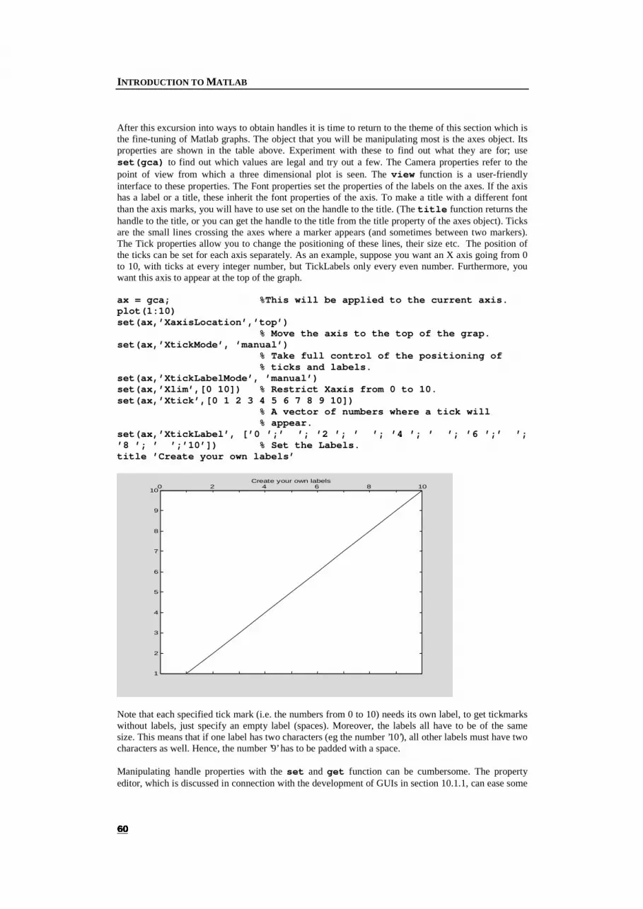
INTRODUCTION TO MATLAB
� �
After this excursion into ways to obtain handles it is time to return to the theme of this section which is the fine-tuning of Matlab graphs. The object that you will be manipulating most is the axes object. Its properties are shown in the table above. Experiment with these to find out what they are for; use set(gca) to find out which values are legal and try out a few. The Camera properties refer to the point of view from which a three dimensional plot is seen. The view function is a user-friendly interface to these properties. The Font properties set the properties of the labels on the axes. If the axis has a label or a title, these inherit the font properties of the axis. To make a title with a different font than the axis marks, you will have to use set on the handle to the title. (The title function returns the handle to the title, or you can get the handle to the title from the title property of the axes object). Ticks are the small lines crossing the axes where a marker appears (and sometimes between two markers). The Tick properties allow you to change the positioning of these lines, their size etc. The position of the ticks can be set for each axis separately. As an example, suppose you want an X axis going from 0 to 10, with ticks at every integer number, but TickLabels only every even number. Furthermore, you want this axis to appear at the top of the graph. ax = gca; %This will be applied to the current axis. plot(1:10) set(ax,’XaxisLocation’,’top’)
% Move the axis to the top of the grap. set(ax,’XtickMode’, ’manual’)
% Take full control of the positioning of % ticks and labels.
set(ax,’XtickLabelMode’, ’manual’) set(ax,’Xlim’,[0 10]) % Restrict Xaxis from 0 to 10. set(ax,’Xtick’,[0 1 2 3 4 5 6 7 8 9 10])
% A vector of numbers where a tick will % appear.
set(ax,’XtickLabel’, [’0 ’;’ ’; ’2 ’; ’ ’; ’4 ’; ’ ’; ’6 ’;’ ’; ’8 ’; ’ ’;’10’]) % Set the Labels. title ’Create your own labels’
0 2 4 6 8 10
1
2
3
4
5
6
7
8
9
10
Create your own labels
Note that each specified tick mark (i.e. the numbers from 0 to 10) needs its own label, to get tickmarks without labels, just specify an empty label (spaces). Moreover, the labels all have to be of the same size. This means that if one label has two characters (eg the number ’10’), all other labels must have two characters as well. Hence, the number ’9’ has to be padded with a space. Manipulating handle properties with the set and get function can be cumbersome. The property editor, which is discussed in connection with the development of GUIs in section 10.1.1, can ease some
CHAPTER 6: GRAPHICS
� �
of this interaction. If you find yourself setting the same properties of figures over and over again, however, you are probably better off writing a script that uses set and get to do this for you (see exercises). Also, in the next version of Matlab (5.3), the plot editor will be introduced to take care of some of the fine-tuning; have a look at the help files when 5.3 is installed.
���� 3ULQWLQJ�DQG�([SRUWLQJ�*UDSKLFV�
There are several ways in which Matlab can produce hardcopy output. The easiest way is to go to the File menu in a figure window and select Print. This will pop up the standard Windows print dialog, which means that all printers available for printing in, say, Word are available here too. This includes network printers. For the end-user this should be all they need. To set this up, however, there is a bit of extra work for the administrator. Matlab gets its connection to the windows print dialog from the settings in the printopt.m file, which can be found in the matlab\toolbox\local directory. Here the default device should be changed to: ’-dwinc’ . In printopt this is done after the line: %---> Put your own changes to the defaults here (if needed) pcmd = []; dev = ’-dwinc’; This setting will, by default, route all print commands through the Windows printer drivers. Note the ’c’: ’dwin’ by itself will always generate black and white output: even if your printer is colour-capable. If Windows is installed properly, this is usually the best thing to do. Once this has been set in printopt, command line print commands will also by default go through windows. Printing from the Figure window has the further advantage that you can set the page position, size and other properties of the hardcopy by selecting ’File|Page Position’ If Windows does not print your figure correctly or if you have special demands, such as Encapsulated Postscript output or Adobe Illustrator output, you will have to print from the command line. The command print takes several arguments. The most important is the driver that is to be used. Standard Colour-Windows printing is obtained by print -dwinc. Other useful drivers are the Postscript drivers of which there are level one and level two varieties -dps, -dps2 and black and white and colour -dps, -dpsc. Moreover, there is a useful driver for Encapsulated Postscript (-deps,-deps2,-depsc,-depsc2) and one for Adobe Illustrator format (-dill). The latter format is useful if you want to post-process your figure in Adobe Illustrator, to add that final touch. There is another issue for those few European users of Matlab; printing is on US letter paper by default. To change this default, go into the matlabrc.m file found in the matlab\toolbox\local directory and uncomment the line saying set(0,’DefaultFigurePaperType’,’a4letter’). A problem with legends is that they tend to change fontsize when printed. To prevent this from happening, force their fontsize by setting it explicitly with a set command like set (findobj (h, ’type’, ’text’, ’FontUnits’, ’points’, ’FontSize’, 10). ������ /DWH[�
Latex works best with figures in Encapsulated Postscript format. LaTeX does not care about level 1 or level 2, but generally, level 2 gives smaller files and better results on most modern printers. If you have problems printing, try level 1. Although Matlab has the option to include a preview bitmap of the figure in the eps-file (-epsi or –tiff) this should be avoided when used in combination with LaTeX. Hence, use print -deps2 filename.eps. Note that this command will overwrite any existing file with the same name without warning! (See exercises) ������ :RUG���3RZHU3RLQW�
Figures can be copy-and-pasted from the Matlab figure window into Word (and most other MS-Windows based packages with the exception of Adobe Illustrator, for which the -dill driver exists). Before you do this, be sure to check the Preferences in the File menu of the figure. Select "Windows Metafile" as the copying format on the Copying Options tab page. Click on the figure, select File|Copy or press Ctrl-C, go to the Word document and select Edit|Paste or Ctrl-V. The figure will appear in the document and can be scaled and moved at will. If you want to edit the figure, right-click it, select
INTRODUCTION TO MATLAB
� �
ungroup and confirm that you want to convert this figure into a Microsoft Office drawing. From then on you can move individual lines, change the labels, fonts and even the datapoints! This ungrouping will not work with three dimensional drawings or with pcolor plots. These ignore the copying options and are always copied and therefore imported as bitmaps which cannot be edited (except in programs like PhotoPaint, PhotoShop, Paintbrush…?). Another way of getting figures into MS-Office is the round-about way through Adobe Illustrator, or another vector drawing package for post-processing. In that case, print the files to Illustrator format (-dill), load this into Adobe Illustrator and from there save it with a preview image. The latter will be visible but not looking all too well in Word, but when you print the document the real image is used. You do need a postscript printer for this to work. Note also that Adobe Illustrator cannot receive figures with copy and paste; you have to print them in the –dill format.
���� )XUWKHU�5HDGLQJ�
The Mathworks devotes a whole book to the graphical possibilities of Matlab. This includes a full discussion of the standard two and three-dimensional plots referred to above, but also techniques to edit bitmap images, develop 3D models with patch-techniques, and even animation. The graphics manual also discusses the ins and outs of graphic handles.
���� ([FHUFLVHV�
1. In the example to make your own tick labels, the labels were spelled out one-by-one and padded with spaces. Define a function that takes three arguments: the handle to the axes, the vector of ticks, and the vector of labels (as numbers or as strings). The function should add the labels to the ticks on the specified axes. To test your function, see the example on page 60.
2. Make the function defined in exercise 1 more flexible. Allow the specification of a 4th argument to select the x,y or z axis for adding the labels. Write the function such that the axes default to the current axes and the label vector to the values of the ticks. Be sure to include error-handling routines in this, as much can go wrong.
3. Make a bar chart with reaction time data (500,300 400ms) for 3 subjects. Write the subjects initials (B,V,Ph) below their respective performance. All text should be in Times-Roman, and the title should be italic.
4. Printing to file does not check whether the file already exists. Write a function (safePrint) which takes two arguments: the format (eps1 or eps2) and the filename (with or without extension). The function should issue a warning if the file exists and ask the user to overwrite. The file extensions should default to '.eps'.
5. When you create a plot with many subplots, the title function will always refer to the current subplot. In many cases, however, you may want to add a title to the figure as a whole. Create a function called supertitle that implements this. Supertitle takes a single string (the title) as its argument.
6. The Matlab graphics manual has descriptions of many additional plotting functions including 3D modelling and animations and the details of some of the functions described here: read it! (\matlab\help\pdf_doc\matlab\graphg.pdf)
� �
�� 'DWD�$QDO\VLV�
All subjects up to now have been preparation for the real work that Matlab does. I will discuss some of the possibilities that I consider most useful to neuroscientists in this section. A complete overview of what Matlab can do is impossible to give here. Even though data-analysis may soon become very specilaised, there are many functions or problems that crop up in very different applications. I cannot stress it often enough: browse through the (online) help, the Matlab user contributed files and the user’s guides before you start programming something from scratch. There is a good chance that something very much like what you want is already part of Matlab or one of the toolboxes.
���� 6WDWLVWLFV�
Matlab pure is (surprisingly) not very good at statistics and the Statistics Toolbox does not do all that much to change this. The basic tests are available, but for something slightly more advanced than an ANOVA, you will have to use SPSS anyway, or write the algorithm yourself. Writing statistical tests yourself is simplfied by a fairly large collection of probability density functions (such as the chi-squared, F, Gamma etc). Taken together with a copy of Numerical Recipes in C you can do it yourself. This has the added advantages that you may actually come to understand that test you have been using all along. Simple functions such as mean(), median(), std() , min() and max() work the way you would expect them to. Given a vector they determine mean, median, standard deviation, minimum and maximum value. Given a matrix, they do this for each column. Built-in tests are the Z-test which compares the mean of a sample (with a known standard deviation) to a constant. ztest(data, testMean,sigmaData,confidenceLevel,tail) All statistical tests return a 1 if the hypothesis is to be rejected at this significance level, a 0 otherwise. A second output argument contains the significance level at which the hypothesis could be rejected. Example: data = randn(10,1); % Take a sample of 10 from the normal
% distribution. [H,significance] = ztest(data,1,1,0.05,0)
% Test whether the mean is different from 1. H = 1 significance = 0.0023 From this test we can conclude that the mean of our sample is different from 1 with a level of confidence p= 0.0023. Next is the T-test for a single sample (with unknown standard deviation): ttest(data,testMean,confidenceLevel,tail) Example: [H,sig] = ttest(data,0,0.05,0) H = 0 sig = 0.8967 The t-test failed: you cannot conclude that these data have a mean unequal to zero. The T-test for two samples allows you to compare the means of two measured datasets: ttest2(dataSetOne,dataSetTwo,confidenceLevel,tail) Example: data1 = randn(100,1);
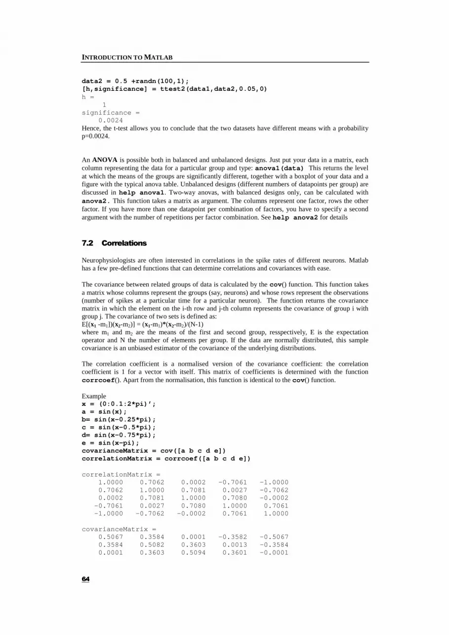
INTRODUCTION TO MATLAB
� �
data2 = 0.5 +randn(100,1); [h,significance] = ttest2(data1,data2,0.05,0) h = 1 significance = 0.0024 Hence, the t-test allows you to conclude that the two datasets have different means with a probability p=0.0024. An ANOVA is possible both in balanced and unbalanced designs. Just put your data in a matrix, each column representing the data for a particular group and type: anova1(data) This returns the level at which the means of the groups are significantly different, together with a boxplot of your data and a figure with the typical anova table. Unbalanced designs (different numbers of datapoints per group) are discussed in help anova1. Two-way anovas, with balanced designs only, can be calculated with anova2. This function takes a matrix as argument. The columns represent one factor, rows the other factor. If you have more than one datapoint per combination of factors, you have to specify a second argument with the number of repetitions per factor combination. See help anova2 for details
���� &RUUHODWLRQV�
Neurophysiologists are often interested in correlations in the spike rates of different neurons. Matlab has a few pre-defined functions that can determine correlations and covariances with ease. The covariance between related groups of data is calculated by the cov() function. This function takes a matrix whose columns represent the groups (say, neurons) and whose rows represent the observations (number of spikes at a particular time for a particular neuron). The function returns the covariance matrix in which the element on the i-th row and j-th column represents the covariance of group i with group j. The covariance of two sets is defined as: E[(x1 -m1])(x2-m2)] = (x1-m1)*(x2-m2)/(N-1) where m1 and m2 are the means of the first and second group, resspectively, E is the expectation operator and N the number of elements per group. If the data are normally distributed, this sample covariance is an unbiased estimator of the covariance of the underlying distributions. The correlation coefficient is a normalised version of the covariance coefficient: the correlation coefficient is 1 for a vector with itself. This matrix of coefficients is determined with the function corrcoef(). Apart from the normalisation, this function is identical to the cov() function. Example x = (0:0.1:2*pi)’; a = sin(x); b= sin(x-0.25*pi); c = sin(x-0.5*pi); d= sin(x-0.75*pi); e = sin(x-pi); covarianceMatrix = cov([a b c d e]) correlationMatrix = corrcoef([a b c d e]) correlationMatrix = 1.0000 0.7062 0.0002 -0.7061 -1.0000 0.7062 1.0000 0.7081 0.0027 -0.7062 0.0002 0.7081 1.0000 0.7080 -0.0002 -0.7061 0.0027 0.7080 1.0000 0.7061 -1.0000 -0.7062 -0.0002 0.7061 1.0000 covarianceMatrix = 0.5067 0.3584 0.0001 -0.3582 -0.5067 0.3584 0.5082 0.3603 0.0013 -0.3584 0.0001 0.3603 0.5094 0.3601 -0.0001
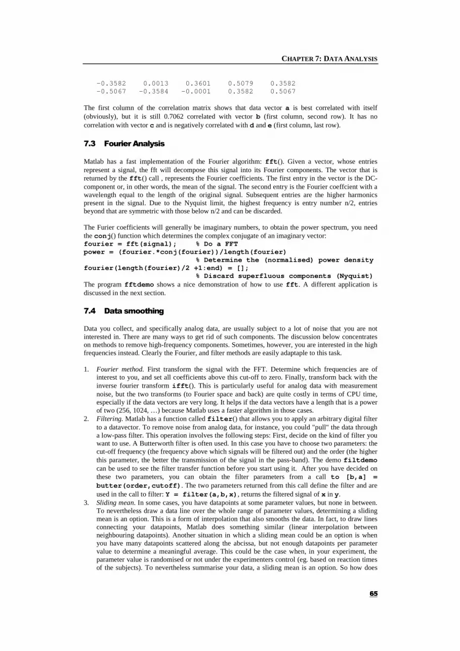
CHAPTER 7: DATA ANALYSIS
� �
-0.3582 0.0013 0.3601 0.5079 0.3582 -0.5067 -0.3584 -0.0001 0.3582 0.5067 The first column of the correlation matrix shows that data vector a is best correlated with itself (obviously), but it is still 0.7062 correlated with vector b (first column, second row). It has no correlation with vector c and is negatively correlated with d and e (first column, last row).
���� )RXULHU�$QDO\VLV�
Matlab has a fast implementation of the Fourier algorithm: fft(). Given a vector, whose entries represent a signal, the fft will decompose this signal into its Fourier components. The vector that is returned by the fft() call , represents the Fourier coefficients. The first entry in the vector is the DC-component or, in other words, the mean of the signal. The second entry is the Fourier coeffcient with a wavelength equal to the length of the original signal. Subsequent entries are the higher harmonics present in the signal. Due to the Nyquist limit, the highest frequency is entry number n/2, entries beyond that are symmetric with those below n/2 and can be discarded. The Furier coefficients will generally be imaginary numbers, to obtain the power spectrum, you need the conj() function which determines the complex conjugate of an imaginary vector: fourier = fft(signal); % Do a FFT power = (fourier.*conj(fourier))/length(fourier)
% Determine the (normalised) power density fourier(length(fourier)/2 +1:end) = [];
% Discard superfluous components (Nyquist) The program fftdemo shows a nice demonstration of how to use fft. A different application is discussed in the next section.
���� 'DWD�VPRRWKLQJ�
Data you collect, and specifically analog data, are usually subject to a lot of noise that you are not interested in. There are many ways to get rid of such components. The discussion below concentrates on methods to remove high-frequency components. Sometimes, however, you are interested in the high frequencies instead. Clearly the Fourier, and filter methods are easily adaptaple to this task. 1. Fourier method. First transform the signal with the FFT. Determine which frequencies are of
interest to you, and set all coefficients above this cut-off to zero. Finally, transform back with the inverse fourier transform ifft(). This is particularly useful for analog data with measurement noise, but the two transforms (to Fourier space and back) are quite costly in terms of CPU time, especially if the data vectors are very long. It helps if the data vectors have a length that is a power of two (256, 1024, …) because Matlab uses a faster algorithm in those cases.
2. Filtering. Matlab has a function called filter() that allows you to apply an arbitrary digital filter to a datavector. To remove noise from analog data, for instance, you could "pull" the data through a low-pass filter. This operation involves the following steps: First, decide on the kind of filter you want to use. A Butterworth filter is often used. In this case you have to choose two parameters: the cut-off frequency (the frequency above which signals will be filtered out) and the order (the higher this parameter, the better the transmission of the signal in the pass-band). The demo filtdemo can be used to see the filter transfer function before you start using it. After you have decided on these two parameters, you can obtain the filter parameters from a call to [b,a] = butter(order,cutoff). The two parameters returned from this call define the filter and are used in the call to filter: Y = filter(a,b,x), returns the filtered signal of x in y.
3. Sliding mean. In some cases, you have datapoints at some parameter values, but none in between. To nevertheless draw a data line over the whole range of parameter values, determining a sliding mean is an option. This is a form of interpolation that also smooths the data. In fact, to draw lines connecting your datapoints, Matlab does something similar (linear interpolation between neighbouring datapoints). Another situation in which a sliding mean could be an option is when you have many datapoints scattered along the abcissa, but not enough datapoints per parameter value to determine a meaningful average. This could be the case when, in your experiment, the parameter value is randomised or not under the experimenters control (eg. based on reaction times of the subjects). To nevertheless summarise your data, a sliding mean is an option. So how does

INTRODUCTION TO MATLAB
� �
this work? Imagine sliding a window over the abcissa. When the window is at the far left, you determine the mean of all the datapoints that can be seen in the window (this of course depends on the width of the window). This mean is the sliding mean for the far-left position on the abcissa
(and is plotted there). Next you shift the window some distance (the step size) to the right and again determine the mean of all datapoints visible inside the window, this is the value corresponding to the current position of the window. By sliding the window over the whole x.axis, you get estimates of the values at all required parameter values. Be aware though that the actual values you find depend on the width of the window and the stepsize of your slides.
���� 2SWLPL]DWLRQ�
The Optimization Toolbox gives access to a number of solution finding routines, usually realted to minimum or maximum finding or zero finding. The function leastsq() is generally useful to find the best parametrised approximation to a dataset. The main advantage over regress() or fit() is that leastsq() allows you to specfiy non-linear relations between parameters and data. The disadvantage is, of course, that no solution can be guaranteed for your optimization problem and, moreover, that if a solution is found it need not be the optimal solution (local minima problem). One can reduce (but not overcome) these problems by starting the leastsq() routine from different starting points. The leastsq() function finds the parameters for which a function specified as the first argument attains its minimum value. Note that this function has to be a Matlab m-file. Assume for instance that you defined a function m-file as in Listing 7-1:
function value = goal(x) value = (x’*x).^3;
� /LVWLQJ�����/HDVW�6TXDUHV�2SWLPLVDWLRQ�
and pass this function to the leastsq() function: leastsq(’goal’,[1 1 2 3]) then leastsq would first pass the vector [1 1 2 3] to the goal function, to evaluate its value. By gradient descent, the leastsq function then determines whether there are any vectors near [1 1 2 3] whose goal-value is lower. If so, this vector becomes the next value. This process is repeated until no vector can be found whose goal value is lower than the last found value.
���� &XUYH�)LWWLQJ�
The statistics toolbox contains the function regress() which takes a vector of observations y and a matrix X as its arguments and returns a vector b such that y = Xb. By supplying the appropriate matrix X, a completely general linear regression can be set up. Confidence limits on the correlation coefficient as well as on the parameters b can be obtained by specifying output arguments. In regression you want to express your data as a function of some known (expected) function. The simplest example of such a function is a polynomial. Assume you have a dataset (y) whose dependence on a parameter (x) looks a lot like a parabola. A linear regression will allow you to determine how well these data are described
Original Data
Sliding Mean Step Size
Window Width

CHAPTER 7: DATA ANALYSIS
� �
by a parabola and will also give you the parameters of the best-fitting parabola. In more mathematical terms, you want to determine the b-parameters in the expression y = b0 +b1x +b2x
2 that lead to the smallest possible discrepancy between the value of the function and the actually measured data. The functions 1,x,x2 are called the basis functions of the regression. Matlab can determine the best fitting b-parameters if you tell it the values of your data (y) and the values of the basis functions at those parameter values (x). An example will clarify this. Assume that you have 2 datapoints (too few to do a regression on a parabola, but as an example, it will do), at x= 1, 2. The measured datavalues are y = 3, 12. You tell Matlab about the values of the three basisfunctions at the three values of x by specifying a design matrix X. The entry X11 represents the value of the first design function at the first parameter-value, X21 the second basis function at the first parameter value. Hence, in this example: X = [1 1 1; 1 2 4; 1 3 9;1 4 16] yData = [3 7 12 20]’; X = 1 1 1 1 2 4 1 3 9 1 4 16 With these parameters, you can call the regress function: [b,bConfidence,r,rConfidence,stats] =regress(yData,X,0.05) WARNING: the stats toolbox seems to be buggy, the regress function does not work (not in Matlab 4.2 nor in 5.2)! In absence of a (working) Statistics Toolbox, the function ’fit()’ in bkTools can be used for general linear regressions and particularly simple polynomial and exponential fits. This function returns fitting parameters, chi-quared statistics and the covariance matrix of the fit. In its simplest form, the fit function asks for the y and x data, the (expected) standard deviations of these datapoints and the order of the polynomial to which you want to fit these data. An example: x = (1:5); y = [2 4 6 7 11]; stdDev = 0.5; [coefficients,covariance,chiSquared,Q]= fit(y,x,stdDev,’p’,1) This model almost seems reasonable coefficients = -0.3000 2.1000 covariance = 0.2750 -0.0750 -0.0750 0.0250 chiSquared = 7.6000 Q = 0.0826 Which tells you that the function y=-0.3 +2.1*x is a reasonably good fit of the data. The goodness-of-fit is given by the χ2 = 7.6. The probability that a χ2 value as poor as 7.6 should occur by chance is Q = 0.0826. Interpreting this number requires some handwaving. NRC says that if Q is larger than 0.1, the fit is believable, values down to 0.001 could be allright if the errors in your measurement procedure (given by the standard deviation supplied to the fit function) are slightly underestimated. More advanced functions, including non-linear curve fitting can be found in the Optimization Toolbox, see help optim, the Matlab Helpdesk and section 7.5.
���� ([FHUFLVHV�
1. Write a function that, given a datavector, window width and step size, determines the sliding mean of the data. The output vector should have the same size as the input data vector.

INTRODUCTION TO MATLAB
� �
2. Extend the sliding mean function such that it can take a weighted sliding average: this means that when determining the mean of the data inside the window, the datapoints nearest to the current position (centre of the window) contribute more than those at the edges of the window. Use a Gaussian weighting function whose "standard deviation"is given by the width parameter. Introduce an optional fourth parameter in the function call, which can be used to select this weighing function.
3. The fit function allows you to do a general linear regression by specifying ’d’ mode. In this mode you have to determine the design matrix (explained on page 67). To test this function, generate a set of data points on the interval 0 to 10 consisting of a weighted sum of three functions, say three Gaussian functions with different widths and centres. Now add some random noise to the data. After this preparation, try to extract the coefficients with which the data were constructed by setting up the design matrix for the three basis functions and running it with the data through the fit function.
� �
�� )LOH,2�
This section deals with the in and output of Matlab. First I will discuss how to store data from a Matlab session to be used later. This includes data which are stored in matrices, but also more complicated objects such as figures. Secondly I will discuss some methods that can be used to retrieve data from other programs (including data-recording programs). After analysing these data you may want to export the results to a format that specialised statistics programs can read, this is discussed in the last section.
���� 6WRULQJ�0DWODE�5HVXOWV�
������ 'DWD�
As briefly discussed in section 3.1 a Matlab matrix can be saved to a file by typing save filename variableName1 variableName2 This stores the variables in a Matlab format which is difficult to decipher by other programs. For export to programs such as Excel, see section 8.3.1. If you want to save your whole Matlab session (i.e. all the variables currently in scope, including the global variables) just type save filename Next time, when you want to continue working on these data, just type load filename to continue where you left off. ������ )LJXUHV�
Figures can be saved from their menubar. Selecting File|Save will prompt you for a filename. This can be a useful way to store the results of a long analysis, together with the fine-tuning that you may have done to get the figure to look just right. Saving it as a Matlab figure will allow you to continnue editing at some later time, this would not have been possible if you printed the figure to file. When you try to save the figure again Matlab will prompt you for another filename, to save it to the same name, just select the filename and confirm the "overwrite" prompt. To open this figure, just type its name: you can treat it as just another m-script. Apart from being a future proof way of storing the results of an analysis, saved figures can also be used as base figures on which similar data are plotted. You could, for instance, prepare a figure with labels, titles, colours etc, call this ’fancyPlot’ and instead of running the command ’figure’ before plotting a new dataset, type ’fancyPlot’ to open a new copy of your fancy figure. Issuing the plot command afterward will simply add the new data to the pre-fab figure. Saving figures is also necessary in the development of GUIs. GUIs in Matlab are nothing more than fancy figure windows that respond to mouseclicks in various ways. This is discussed in detail in section 1.
���� ,PSRUWLQJ�'DWD�
Many programs generate ASCII or text files as output. If the data in the file is space-separated and the number of elements on each row is the same (i.e. it is a matrix) you can use the load command to read the file. load -ascii filename If the file contains rows of different length, this easy data reading is not possible. In this case you could use the fgets function, which reads one line after the other from a file. To use this, you first have to open the file and get a handle to its contents: fileHandle = fopen(’filename’) found = 0; while found <> -1
INTRODUCTION TO MATLAB
� �
found = fgets(fileHandle) end fclose(fileHandle) This code snippet first opens the file, then reads the lines one by one and stores this in the variable found. When the fgets function has found the end of the file, it returns the value -1 and stores this in found. At that point the while loop terminates and the file is closed. Try it on a simple text file! Don’t forget to issue the fclose command, otherwise you may have trouble later on, in another program, to open this file. Moreover, open files take up resources and are more prone to corruption than closed files. With an fgets call the returned variable will always contain strings representing the current line in the file. If a line contains more than one number, all numbers will be part of this string. Usually, however, you will want to store the various numbers on a line in different variables. The numbers may represent different aspects of a stimulus, such as the speed, luminance and size of a moving object in a display, these numbers would have to be stored in three separate variables. In other circumstances, you may want to store a whole line in the file in a single vector. This may be the case if you have a file that contains the spike times of a cell you recorded electrophysiologically. To read numbers directly into variables. the fscanf function is suitable: [data,numberRead] = fscanf(fileHandle,’%f’); This function reads floating point data from file and returns this in the variable ’data’. The format of the data to be read is specified in by the ’%f’ string. The ’f’ means that you expect to read a floatuing point number, ’d’ would mean an integer. See help fscanf for details. For data stored in a binary format (i.e. those that are not readable in a texteditor) fread should be used. For binary data you specify what you want to read from the file. From the program that generated the file you obtain the information about the format: for instance, a program stores 5 single precision floating point numbers, then two integers, and finally a short in a file. Reading this would go as follows: fileHandle = fopen(filename,’r’); % open for reading data1 = fread(fileHandle,5,’float’); % Read 5 floats data2 = fread(fileHandle,2,’int’); % read 2 integers data3 = fread(fileHandle,1,’short’) % read 1 short fclose(fileHandle) % Close the file This will store the data in the variables data1, data2, data3. To check whether your data reading operation was successful, you could check the length of the data vectors or look at the second output argument of the fread function which tells you the number of numbers read. You have to be very careful when reading binary files: be sure to follow the definition of the format of the file to the letter. Reading files with the wrong size specifier (i.e. reading an int as a float) will lead to complete nonsense numbers in your data. (Numbers such as 1e+109 in a vector that was read from a binary file are an almost sure sign that your file reading routine is incorrect). Apart from the wrong size specifier, errors do occur due to differences in binary formats. Matlab’s default is to read data in the format that the machine on which the program runs uses. I.e. if you run Matlab under Windows on a PC, it will use a PC format. This spells trouble when you import data generated under Unix, where the byte ordering of binary numbers is (sometimes) reversed. Silicon Graphics Irix, for instance, uses ’big-endian’ byte ordering. To open a file generated on an SGI, you must speciffy this ordering to the fopen function: fileHandle = fopen(filename ,’r’,’b’) % Open file from SGI. Note that it does not matter where the file is stored, it matters which operating system (or even program) was used to generate this file. If nonsense numbers show up in your data, this is another thing to keep in mind.
���� ([SRUWLQJ�'DWD�
Matlab is flexible and powerful, but some things such as a thorough statistical analysis are more easily done in specialised packages such as Excel or SPSS. Moreover, the possibilities to generate graphs in a

CHAPTER 9: DATASTRUCTURES AND OBJECT ORIENTED PROGRAMMING
� �
more intuitive, interactive manner are well developed in Excel. Use Matlab for the things it does best: simulations, long heavy calculations, complicated maths, but use Excel or SPSS when it comes to statistics. To be able to use your data in these other packages, you will have to export them. All three packages can read ASCII data. This means that you can export a data matrix to a file by using the save function with the –ascii option and simply open this file in any of the packages. One important thing to note here is that the number of data columns that these programs read is restricted (Excel97 reads 256, for instance). If your file contains more columns these are simply discarded: no warning is issued by any of the programs and you simply loose your data. If the number of rows in your data matrix is smaller than 256, you can circumvent this problem by rotating the matrix. If the number of rows is also larger than 256, you will have to split the analysis up into parts. ������ ([FHO�
Excel and Matlab can communicate through DynamicData Exchange. This is an MS-Windows protocol that allows the exchange of data between two running applications, without the need for any files. With DDE, you can link a range of cells in Excel to a matrix in Matlab. This link can be live: whenever the matrix changes in Matlab, the cells in Excel are automatically updated. The Excel macro toMatlab in the bkTools.xls add-in is somewhat simpler, it allows you to push ranges from Excel to a named Matlab matrix, and vice versa to retrieve a matrix from Matlab and write its entries to a specified range of Excel cells.
���� ([FHUFLVHV�
1. Write error-handling routines that issue a warning if a file could not be opened for reading or writing. As this is a routine that is useful in many applications, write it as a separate function, called safeOpen, which takes a filename and a mode-string as its argument and which returns the fileHandle. Make the error-messages user friendly: determine the cause for the error (does the file exists at all?, is it open already?, is it in binary/text format?)

INTRODUCTION TO MATLAB
� �
�� 'DWDVWUXFWXUHV�DQG�2EMHFW�2ULHQWHG�3URJUDPPLQJ�
One of the rules that lead to successful programming is to "keep together what belongs together". This rule can be applied to the whole hierarchy of programming objects. Starting at the top, you should keep M-files that tackle similar problems together in a single directory. This makes it easier for you to find these functions. Moreover, when you start programming a new function from the same cateegory, you can have a quick look to see whether you already programmed something that was similar and may be adapted or extended. Finally, in combination with the what function, you can quickly find out what functions are available in this general category. One step down, scripts should deal with tasks that form a logical entity. If you have subtask that stand quite apart from the rest, separate them out from the main script and write them as other small scripts, or better even as functions that can be used by future scripts as well. Writing programs this way allows you to keep an overview of the main structure of your program (in the main script) without looking at the details of all the subtasks. This makes spotting errors in the logic of the program much easier. Conversely, you can edit the scripts that deal with particular tasks on their own, without being concerned with their particular embedding in the larger whole. This, however, will only work if you stick to local variables in your functions, otherwise unexpected dependencies could arise between subtasks and the main program. Further down, we find the parts of a single script. Again, separate those parts concerned with different aspects of the task visually: use written comments, but also lines between parts of the code that are relatively independent (but not so independent that they could be written as a separate script).
���� 1�GLPHQVLRQDO�$UUD\V�
At the lowest level we find the variables that Matlab works with. Up till now we have been working with scalar, vector and matrix variables. They already part of the "keep together what belongs together" philosophy. For instance, using a matrix to store the data of five subjects on the same task keeps those data together in one place. This is much more transparent than the alternative way where you would define five vector variables that each contained the data for one subject. The scalar, vector, matrix ladder can be extended to N-dimensional arrays. These arrays work just like matrices, except that beyond rows and columns, they also have so-called pages. For a three-dimensional array you can still visualise this, but not for a four dimensional array. A three dimensional array would, for instance, be useful to store all results from two groups of five subjects who did the same experiment 10 times. You would need a matrix with size [2 5 10] for that. The result of the second subject from the first group on the 5th experiment would be given by data (1,2,5). It is as simple as that. Of course, having such an array, rather than many vectors, makes it much easier to do the same calculation for all subjects in all groups. For-loops are often used in conjunction with N-dimensional arrays to apply a certain operation to certain lower-dimensional slices of the array (eg. the slice that has all the subjects of group 1: data(1,:,5)) The trouble with N-dimensional arrays is that not all data fit in such a regular array: to form an array, the number of elements has to be the same in all dimensions. In the example above if the second group had only 4 subjects, while the first had 5, an N-dimensional array could not store the data without resorting to some default values for the "absent subject". Luckily, cell arrays have no such restriction on the dimensions and they too can be N-dimensional. I.e. to keep the spike times of two cells recorded on 15 trials of 5 conditions, you would use a cell array called spikeTimes. spikeTimes would have size 2*5*15, and each element would be a vector of a length equal to the number of spikes that that particular cell fired in that trial and under that condition. In fact, one could argue that this is a 4 dimensional object, where the 4th dimension is the spiketime. This dimension is not equally large for each of the other three dimensions. For instance, if cell 2 fired 5 times at [100 110 120 130 200] ms in trial 5 of condition 1: spikeTimes{2,5,1} = [100 110 120 130 200]. Note the curly brackets used to subscript into the cell array. To access the second spike time, type: spikeTimes{2,5,1}(2). Here we have four subscript references to extract a scalar number from a four-dimensional object. The first three numbers, in the curly brackets, subscript into the 3D cell array and extract a 1D vector. The last number, in the normal parenthesis, subscripts into this 1D vector and extracts the element.

CHAPTER 9: DATASTRUCTURES AND OBJECT ORIENTED PROGRAMMING
� �
These N-dimensional data structures are useful to keep very similar data together, especially data that you may want to apply the same analysis to. Referring to particular elements can sometimes become somewhat confusing. This is even more so when the data you wan to store are related but not of the same type. Consider for instance a recording where you subjects detection thresholds as a function of stimulus luminance, but also their reaction times. I.e. how fast they detected the stimulus. As these quantities are quite different you will probably not want to apply the same analysis to both (except maybe simple things like determining the mean). Nevertheless, these data belong together, hence they should stay together. You could choose to store them in the different pages of a three dimensional array, but you would have to be very careful not to access the detection thresholds of subject 2 in experiment 3 (data(1,2,3)) when you wanted the reaction times (data(2,2,3)). There is nothing in this notation that makes it clear what you are accessing and hence it leads to the same problems as the use of cryptic variable names. Matlab 5 borrowed an elegant solution for this kind of problem from C that can make your code much more readable: structures.
���� 6WUXFWXUHV�
A structure is an object with elements that can be referenced by name. For the example above, we could define the structure ’data’, which has fields ’reactionTime’ and ’detectionThreshold’. These fields can be defined simply by asssigning data to them: data.reactionTime = [200 300 200 300 405]; data.detectionThreshold = [0.3 0.4 0.1 0.4 0.2]; Now the structure data contains two vectors that can be referenced by their names and treated as any ordinary vector. To extract the second element for instance data.reactionTime(2) ans = 300 or, to determine the mean: mean(data.reactionTime) ans =281 Hence structures allow you to store properties of objects together. In this example we have stored the results of one experiment in the data structure, but we could also add the name of the subject, her age, the day at which this experiment was done and any other information that pertains to this experiment in this datastructure: data.subject = ’PP’; data.age =29; data.date = ’01-04-99’; The information stored in the variable data can be retrieved just like any other variable, by typing it at the command prompt. This will, however, only show those elements that are easy to display: strings and vectors, but not matrices. For matrices contained in the structure, only the size is shown. data
reactionTime: [200 300 200 300 405] detectionThreshold: [0.3000 0.4000 0.1000 0.4000 0.2000] subject: ’PP’ age: 29 date: ’01-04-99’ To take this one step further, we can now store the information on many subjects’ performance in the experiment in a vector of structures. For instance: data(2).subject = ’JK’; data(2).reactionTime = [100 200 300 300 200]; data(2).detectionThreshold = [0.2 0.3 0.2]; Now, data is a structure array. The first element of the array is the structure containing the information on subject ’PP’, the second that on ’JK’. To access individual elements of the structure array we can mix subscript addressing with structure referencing and more subscript referencing. For instance, the second reaction time of JK is: data(2).reactionTime(2) ans =200 Or, we can look at the difference in reaction times of the two subjects by: data(1).reactionTime-data(2).reactionTime ans = 100 100 -100 0 205
INTRODUCTION TO MATLAB
� �
Structures allow us to store all information that is relevant to a particular object in one place, in one variable. This is makes your code transparent, because you always know where the information is and where it comes from. Compare for instance the notation subjects(2).reactionTime with data{2,1}. Both could store the same information, but the former, by using sensible variable names and the power of structures is almost normal language and thereofre much easier to understand than the cryptic data{2,1}. Another way of solving this problem is the use of many temporary variables that store the information of the currently active data object. Some operation that looped over all cells in a recording would for instance store the spiketimes of cell number 1 in the variable tmpSpikeTimes, do th eanalysis on this then store the spiketimes of cell 2 in tmpSpikeTimes etc. With structure arrays you would have a single data structure called ’cell’ and write a loop as follows: for cellNr =1:nrCells analyse(cell(cellNr).spikeTimes) end where analyse is some kind of function that analyses the spiketimes. This code speaks for itself. Structures are not only a transparent way to keep information about your data objects together, they also provide for a more transparent way to deal with the many properties of handle graphics objects. The rather cumbersome: set(h,’Color’,’r’,’Marker’,’.’,’LineWidth’,7) can also be written as: the more transparent: lineProperties.color = ’r’; lineProperties.Marker = ’.’ lineProperties.LineWidth =7 set(h,lineProperties) This is particularly useful if you want to use the same properties for many different objects. In that case you only have to define the properties structure once and use it thoughout your program.
���� &ODVVHV�DQG�2EMHFW�2ULHQWHG�3URJUDPPLQJ�
To complete the hierarchy of data structures that embody the "keep it together" philosophy, we have to consider a form of information that we have not considered yet. Up to now, we have talked about static information about data objects: the number of spikes, the number of subjects, the name of the subjects or the date of the experiment. We have seen ways of keeping this static information together. Usually, however, we have a whole range of other information about data that is much more active. For instance, we know how spiketimes should be plotted (as a raster plot and optionally a peri stimulus histogram). Or, if the data object is a data file with a particular format, we know how the data should be read from file for this object. In other words, we know the methods that apply to this object. Object Oriented Programming is the culmination of all techniques discussed in this section: it aims to store passive contents of an object together with the methods that this object can execute. ’Methods’ is another word for functions. I.e. the methods of an object are the M-functions that can be applied to this object. In OO terms, these are the M-functions that the object can execute. This is in fact an easier way of thinking: objects are not passive things that wait until you apply a function to them. Instead, they have a range of methods with which they manipulate themselves and possibly other objects. Some objects, or better classes#, are pre-defined in Matlab. For instance, the class ’double’ contains all normal Matlab matrices, vectors and numbers. The passive contents, or properties, of the objects in this class are simply the numbers in the matrices. The methods of this class are all functions that can be applied to matrices. For instance, the function ’plot’ is one of the methods of the double-class. Similarly, the operators ’+’ and ’*’ are methods of the double-class: the methods define ways in which the objects of this particular type (of this class) can be manipulated.
# An Object is an instance of a particular Class. In other word, the class is an abstract description of a particular kind of object, somewhat like a template. An object is a specific example of something that behaves according to the rules of the Class. In programming, you define a Class, but use Objects in your code.
CHAPTER 9: DATASTRUCTURES AND OBJECT ORIENTED PROGRAMMING
� �
All m-files defining a new class are stored in a single directory with a special name. The name of the directory should be @classname, where classname is an arbitrary name of the class you want to define. This directory itself should not be on the Matlab search path although the parent directory should be. To define your own class, you must first write a special function called the constructor of the class. This function sets up a structure to contain the passive content of the object: it tells Matlab what kind of information will be stored in objects of this class. Secondly, you define the methods that will apply to objects of this class. The constructor as well as the method m-files are stored in the class directory. This is an important way in which all information is kept together and makes maintenance of your code much easier. An example will clarify some of the issues. Consider an experiment in a virtual reality environment in which human subjects are first "driven" to some location and then instructed to find their way home by manipulating a joystick. As part of the analysis, we want to plot the positions that subjects moved to in the two-dimensional plane. To show the variability in their answers over trials, we also want to show the standard deviation over trials as an ellipse around the mean "home position". Analysing the problem, you realise that you will be plotting many ellipses. As this is not a pre-defined function in Matlab and because it is something that may come in useful in other programs as well, you decide to set up a class for this purpose. To completely specify an ellipse, you need its centre, the length of the two axes as well as the orientation of one of the axes. These elements will become the properties of the ellipse class. For plotting purposes, some other properties may be of importance as well. You could for instance define the colour and the linestyle of the ellipse. For our current purposes, we need to define a plot method for this class: this will draw the ellipse on the current figure. We also decide to implement a colour method that changes the colour of the ellipse and a move method, which moves the ellipse by a certain amount. The latter function may come in useful when we want to simulate the temporal dynamics of the user’s response: i.e. how they found their way home. Finally, we will implement a function that returns the surface area of the ellipse. Although this is a general property of ellipses (and hence belongs to the methods of the calss ellipse), it can be used in this particular application to obtain a measure of the uncertainty of the subjects. Table 2 summarises the first step of the class-design process and shows the properties and methods that the ellipse class will need.
@ellipse: ellipse Class constructor. Properties centre The x,y location in the two-dimensional plane shortAxis The length of the short axis. longAxis The length of the long axis. orientation The orientation of the long axis. colour The colour of the drawing Methods plot Plot this ellipse move Move this ellipse to another position. colour Give the ellipse a specific colour. surface Determine the surface of the ellipse
� 7DEOH����7KH�(OOLSVH�FODVV��
������ 7KH�FRQVWUXFWRU��
The second phase of the class design is to capture the definitions in terms of m-files. We start by creating a directory called ’shapes’ and in that directory a subdirectory called @ellipse. Use the path-browser to put the ’shapes’ directory (but not the @ellipse directory) on the search path. Then, create an m-file called ellipse in the @ellipse directory. This m-file will be the constructor function for objects of the ellipse class. The constructor tells matlab what kind of properties this object has and, when called with appropriate arguments, can set the properties of the object. Listing 9-1 shows the typical style of a constructor.
function e = ellipse(centre,short,long,orient) % Constructor of the ellipse class. % Creates an object of the ellipse class with properties: % % centre The x,y location in the two-dimensional plane % shortAxis The length of the short axis.

INTRODUCTION TO MATLAB
� �
% longAxis The length of the long axis. % orientation The orientation of the long axis. % colour The colour of the drawing % % BK - 5/3/99 e.centre = [0 0]; e.shortAxis = 1; e.longAxis = 2; e.orientation = 0; e.colour =’b’; if nargin ==0 %Default constructor. e = class(e,’ellipse’); elseif isa(centre,’ellipse’) %Copy constructor e =centre; elseif nargin ==4 % Initialisation constructor e.centre = centre; e.shortAxis = short; e.longAxis = long; e.orientation = orient; e = class(e,’ellipse’); else error(’No such constructor for an Ellipse’) end
* /LVWLQJ������7KH�FRQVWUXFWRU�RI�WKH�HOOLSVH�FODVV�
The if-then-elseif construction is always necessary in a constructor because a call to the constructor can be done in various ways. The most common call will be the one handled by the last condition (nargin==3). This is a call of the type e1=ellipse([1 1], 2 ,3,45) which is a request to create an object e1 of the class ellipse with its centre at [1 1], a short axis of 2, a long axis of 3 and an orientation of 45. In the constructor function the information passed as arguments is stored in the form of a structure (for instance, the value [1 1] is stored in the ’centre’ field of the object.) . After storing this information, the structure is converted to an object with type ’ellipse’ in the call to class. From now on, Matlab nows that this object (i.e. the object e1) is an ellipse. This means two things. First, all its properties have become essentially private: you cannot type e1.centre as you could with a structure. This information is only available to the class methods. Secondly, by converting the structure to a class, Matlab now knows that when you type plot(e1), it should use the m-file plot.m defined in the @ellipse directory. I.e. it knows which methods apply to this object. Other calls to the constructor occur for instance when you make a copy of an object. When you type e3 = e1 and e1 is an object of class ellipse, the constructor function will be called with nargin==1 and the value of the variable e1 stored in the variable ’centre’. (In this circumstance the latter unavoidably has an undescriptive name). In the constructor above, the e1 object is then simply copied and returned. The default constructor is used when you type e1=ellipse;. This calls the constructor with nargin==0 and in that case the object gets the default properties set in the first lines of the constructor. Because you cannot change the number of properties of an object, it is a good idea to start each constructor with such a list of properties and their default properties, even though this does mean that sometimes code gets executed that is not strictly necessary. ������ &ODVV�0HWKRGV��
After defining the properties of the class in the constructor, we now continue with the methods. The method ’surface’ is a typical example of a method. A method is nothing more than a function that can only be applied to objects from a particular class. Given this object input and optionally some other

CHAPTER 9: DATASTRUCTURES AND OBJECT ORIENTED PROGRAMMING
� �
arguments, the method returns a value. The method is defined just as any other function, as shown in Listing 9-2.
function s = surface(e) % Determines the surface of an ellipse object. % BK – 5/3/99 s = pi*((e.longAxis+ e.shortAxis)/2).^2
� /LVWLQJ�����7KH�6XUIDFH�PHWKRG�RI�WKH�(OOLSVH�FODVV��
Inside one of the methods, the properties of the object are available as if the object were an ordinary structure. Outside the methods, however, objects can only be manipulated as a whole or through their methods. This encapsulation of the data has the advantage that you can be sure that the contents of your dataobject can only be changed by functions that were specifically written for that purpose. After adding the surface.m file to the class directory, you have to force Matlab to update its internally stored functions by typing clear functions. This way the newly added method of the ellipse class will be recognised by Matlab. Moreover, whenever you change the constructor of a class (and hence the internal memory structure of the class), you must delete all objects that were constructed with the old constructor. If you forget to do this, Matlab will complain that you cannot change the class structure. ������ 2YHUORDGLQJ�0HWKRGV�
Apart from functions peculiar to the class being defined, there are some functions that could apply to any class. For instance, most objects will have a plot method. Although the actual results of this method will be different for each object, they are all sensibly called plot methods. For an object of the class ’double’, for instance, the method plot results in a small dot in a figure window, but for an object of the hypothetical class ’spikeData’, it could result in a peri stimulus time histogram. This re-defining of existing methods for a newly defined class is called overloading. Let us habe a look at the overloaded plot method for the ellipse class. Create a file called plot.m in the @ellipse directory and add Listing 9-3. The details of the mathematics are not of particular interest here. What is important, however, is the way in which the information about the object is extracted from the underlying object-structure. Note that the function call only receives the ellipse object (stored locally in the variable e). Inside the method we can refer to the properties of the object by use of the structure notation e.centre, e.orientation etc.
function plot(e) % Plot function for ellipse objects. % % BK – 5/3/99 th = 0:2*pi/100:2*pi; x = e.shortAxis*cos(th)+e.centre(1); y = e.longAxis*sin(th)+e.centre(2); [th,r] = cart2pol(x-e.centre(1),y-e.centre(2)); th = th-e.orientation*pi/180; [x,y] = pol2cart(th,r); x = x+e.centre(1); y = y+e.centre(2); plot(x,y,e.colour)
� /LVWLQJ�����3ORW�PHWKRG�IRU�(OOLSVH�&ODVV��
Even though many plot.m files may be defined on your Matlab search path, Matlab knows that this particular plot method only applies to objects of the class ellipse. Another often overloaded function is the display function. This function is called whenver you type a variable name of a particular class without a semicolon and press return. As you know, for vectors and matrices this will result in their contents being shown at the command prompt. Another way of putting this is that the display-function of the double-class simply returns the numbers contained in that

INTRODUCTION TO MATLAB
� �
double-object. For user-defined classes, the default display function returns a message about the kind of class that this object is part of. For instance: e = ellipse([2 2],1,2,45) e = ellipse object: 1-by-1 Here Matlab reports that e is a single ellipse object. It would be more informative, however, if Matlab could return some or all of the properties of this object. To implement this, you have to overload the display function. To display the centre and the axes of the ellipse, you simply define a function called display in the @ellipse directory along the lines of Listing 9-5.
function display(e) % Display function for ellipse objects. % BK - 5/3/99 disp(’---------------- Ellipse Object ------------’) disp([’ Centre: ’ num2str(e.centre)]) disp([’ Long Axis ’ num2str(e.longAxis)]) disp([’ Short Axis ’ num2str(e.shortAxis)]) disp(’--------------------------------------------’)
� �/LVWLQJ�����2YHUORDGHG�'LVSOD\�0HWKRG�IRU�(OOLSVH�&ODVV�
There are no restrictions to the definitions, if you want to include extensive graphical displays in your display function for a particular classs, you are free to do so. Many other functions can be overloaded as well. To overload a function, you must know what the name of the corresponding m-file is. This is easy for functions such as plot. The corresponding m-file to be defined in the class-directory is plot.m. For operations with no clear link to an m-file, there always is a logically related m-file that can be defined in the class directory. The display.m file is an example of this, other examples are the m-files mtimes.m, plus.m and minus.m that correspond to arithmetic operations suchs as ’*’, ’+’ and ’-’. The m-files corresponding to arithemtic operators can be found under help ops. For our ellipse object we could overload the multiplication operation ’*’. Although the interpretation of the overloaded method is entirely up to the programmer, it makes sense to use arithemtic operators for logically related operations that apply to the particular class. For instance, multiplying an ellipse by a number could be taken to mean the stretching of both axes by the same amount. To implement this, define the method mtimes.m as in Listing 9-5.
function eNew = mtimes(e,number) % Defines ellipse*number as the stretching of both axis of % the ellipse by the same amount. % BK – 5/3/99 if isa(number,'ellipse') tmp =e; e=number; number=tmp; end eNew =e; eNew.shortAxis = e.shortAxis *number; eNew.longAxis = e.longAxis*number;
� /LVWLQJ�����2YHUORDGHG� �RSHUDWLRQ�IRU�(OOLSVH�&ODVV�
The if-end construct in the file swaps around the variables if the command was ’10*ellipse’ rather than ’ellipse *10’, hence it provides additional flexibility in the use of the multiplication operator. Note furthermore how the mtimes function returns a new object, that is a copy of the input ellipse object except for the size of the two axes, which have been scaled by number. small = ellipse([0 0],1,2,0); large = small*10 ---------------- Ellipse Object ------------ Centre: 0 0 Long Axis 20 Short Axis 10

CHAPTER 9: DATASTRUCTURES AND OBJECT ORIENTED PROGRAMMING
� �
-------------------------------------------- ������ 5HDGLQJ�DQG�:ULWLQJ�2EMHFW�3URSHUWLHV�
In the examples up to now, we have determined properties of an object, displayed it numerically and graphically and even derived new objects from it. None of these operations, however, has changed the original object. In the example above for instance, the small ellipse stil has its original radii of 1 and 2. This is the behaviour you would expect from a multiplication operation, but sometimes you will want to change the properties of an object without creating a new object. Because interactions with objects properties can only be done through its methods (the properties are private), the following will not work: small.centre = [1 1] ??? Access to an object’s fields is only permitted within its methods. The work-around for this is to overload the subscripted assignment method. This method is called for structures whenever you type something of the form ’structure.field = value’. The structure data in section 9.2, for instance, has a field called ’name’. Assigning a value to this field by: data.name = ’JK’ results in the following Matlab internal call: subsasgn(data,S,’JK’). In this call the structure S contains information about the kind of subscripted assignment this was. S has the field ’type’, which in this case contains the value ’.’ In order to implement similar assignment procedures for our ellipse object, we have to overload the subsasgn method. Although this may seem like a lot of work for a simple task, it actually makes your code much more robust as you can be sure that changes to your object always take place in the m-files in the class directory. By providing ample error checking in these files you can be sure that no unforeseen changes creep in. For instance, in the ellipse class you could check to make sure that the length of the axes is not negative.
function e = subsasgn(e,S,value) % Subscripted assignment of ellipse objects. switch S.type case ’.’ switch S.subs case ’shortAxis’ if value <0 warning(’Short Axis cannot be smaller than zero’) else e.shortAxis =value; end case ’longAxis’ if value <0 warning(’Short Axis cannot be smaller than zero’) else e.shortAxis =value; end otherwise warning (’This property of an ellipse cannot be set’) end end
� /LVWLQJ�����2YHUORDGLQJ�VXEVFULSWHG�DVVLJQPHQW�IRU�WKH�HOOLSVH�FODVV��
With the overloaded subsasgn.m of Listing 9-6 we can change the ’longAxis’ and ’shortAxis’ properties of an ellipse object: they have become public properties, albeit with some error checking on possible assignments. The other properties on the other hand, still remain private, and will only become public when added to the switchyard in the subsasgn function.
INTRODUCTION TO MATLAB
� �
small.shortAxis =0.5 ---------------- Ellipse Object ------------ Centre: 0 0 Long Axis 2 Short Axis 0.5 -------------------------------------------- Note the crucial return argument of the subsasgn function: the object variable e itself that enters as an argument is returned as an argument. This construct makes sure that the small variable in the default workspace gets its new properties assigned. Subscrpted assignment allows you to write object properties, subscripted reference allows you to read object properties. Hence, if you want to allow read-access to the centre of the ellipse outside the class methods, you should overload the subsref function.
function value = subsref(e,S) % Overload subscript reference for the ellipse class. % Provides access to the centre and surface of the ellipse. switch S.type case ’.’ switch S.subs case ’centre’ value = e.centre;
case ’surface’ value =surface(e); otherwise warning ’This is a no-read property’ value =-1; end end
� /LVWLQJ�����2YHUORDGLQJ�VXEVFULSW�UHIHUHQFH�RI�WKH�(OOLSVH�&ODVV��
Now we can request the centre property of an ellipse object: small.centre ans = 0 0 as well as its surface: small.surface ans = 6.4766 The surface subscripted reference demonstrates that the key you use as a subscript reference need not be one of the properties of the object. You are free to do what you want with particular subscript references, in the current example, the surface reference is interpreted as a call to the surface function. I.e. surface(small) and small.surface are now equivalent. The latter notation is much more like that in C++, is much more readable and seems to be taking over in many programming languages. This notation also stresses the object-oriented viewpoint that the object is doing something in response to your request, rather than the functional/C viewpoint that you do something to the object. As a final example in which some of the issues discsussed on the preceding pages come together, let us have a look at the move function. As mentioned above, this function should move the ellipse by some vectorial (x,y) amount. One way to could this would be to write a method called move that takes the ellipse and the vector as its argument and returns a moved ellipse. I.e something like: movedEllipse = move(e,[1 1]); The problem with this approach is that we now have two ellipses, one at the original position of e and one shifted by 1 in both x an y direction (the latter is stored in the variable movedEllipse). To circumvent this proliferation of ellipses, you could write e = move(e,[1 1]), which simply stores

CHAPTER 9: DATASTRUCTURES AND OBJECT ORIENTED PROGRAMMING
� �
the new ellipse in the same variable as the old (not-moved) ellipse and thereby eliminates the old ellipse. There is a more elegant solution though that can be implemented with subscripted assignment. Suppose we add the following case statement to the subsasgn function:
case ’move’ e.centre = e.centre + value;
� /LVWLQJ� ���� $Q� H[WHQVLRQ� RI� WKH� VXEVDVJQ� PHWKRG� RI� WKH� HOOLSVH� FODVV� �VHH� DOVR�
/LVWLQJ�������
Then we can move an ellipse by typing: small.move = [3 4] ---------------- Ellipse Object ------------ Centre: 3 4 Long Axis 2 Short Axis 0.5 -------------------------------------------- With this implementation of ’move’ you actually move the object itself, without creating any new objects. ������ &DYHDWV�DQG�&RPPHQWV�
When you overload the subsasgn and subsref functions, you not only change the way Matlab treats calls to ’object.field’ , but also object(10). The latter is a subscripted reference too! In this case a call to subsref(A,S) will result with A = object and S.type =’()’ and S.subs = 10. If your subsref function contains no code to deal with this possibility, this operation will be ill defined. For the ellipse class, this should not be a problem as you probably will not be tempted to use the e(5) notation. It is a good idea though to acknowledge the possibility that someone may try to use the class in this way and generate an appropriate error message in the subsref method. For some classes you may want to exploit the possibility to overload index references. You could, for instance, define a class that implements a moving shape. Referencing this as shape(10) could be overloaded to return the shape at time t=10. Defining a class entails quite some overhead: you have to create the appropriate directory structures, define a constructor and usually the display function before you can even start to code the methods to do the real work. Clearly, this overhead only pays off when your class will be used a lot and even more so when this class will be used in various programs. In the latter case you have to make sure that your class is very robust to different ways of calling the methods. Be generous with error messages and flexibility in the method definitions, this will make it easier to use the class in a future program. Objects can be nested, or in OO-speak: aggregated. This means that an object can contain another object as its property. An object that encapsulates the interaction with data from an electrophysiological experiment, for instance, could have a property called trials, which contains an array of trial objects. Each of the trial objects contains data for a single trial. Inheritance is a powerful way to create new classes from existing ones. The classical example is a parent class called shapes, which has a set of properties and methods that are the same for all shapes. The individual shape classes (of which ellipse is only one, we could add circles, squares ,etc.) inherit their structure from the shapes class and add further properties and methods. In practice this means that whenever a method is defined in the class directory of the object, that method is executed. If no method definition is found, Matlab looks for a definition in the parent class directory and executes that method. You can tell Matlab that a class inherits properties from another class when you cal l the class function. For instance: e =class(e,’ellipse’,’shapes’) This tells Matlab that e is an ellipse object whose parent class is the shapes class. You can even add further classes as parents after ’shapes’ for multiple-inheritance. A neuroscience example of this would be the class ’spikeData’ which has properties such as spikeTimes, recordingDate, anaimalName etc. The parent class could implement a method called psth which could plot a psth on the basis of the spikeTimes property. Classes that inherit from this class could for instance be the REXSpikeData or NabedaSpikeData class. These classes encapsulate the interaction with specific spike data recording programs. The methods for reading data from file will be quite different for these different classes, but
INTRODUCTION TO MATLAB
� �
they can both inherit the psth method from their parent. This saves a lot of time on coding, prevents you from having to duplicate a lot of code (and hence make it impossible to maintain) and keeps your analysis flexible in that you can always add further children classes (eg. new dataformats).
���� ([HUFLVHV�
1) The ellipse class used an overloaded ’*’ operation to implement a scaling of the ellipse in all directions. Sometimes, however, you may want to scale the two axes of the ellipse differently. Overload the ’.*’ operator (by redefining times.m in the @ellipse directory) to implement this.
2) Moving ellipses is like adding them to a two-dimensional vector. Hence, it makes sense to overload the ’+’ operator. Use the existing move function in an overloaded plus.m to implement this.
� �
��� *8,�%XLOGLQJ�
When you find yourself using the same program over and over again, switching between the editor (to change some parameters), the Matlab command prompt and an output figure repeatedly, you may contemplate developing a GUI for your application. A good GUI will allow you to change the important parameters of your analysis in an intuitive way, start the analysis and display the results, all in a single window. Good GUIs give an immediate insight into the data, bad ones take up much more processing time than a command line program, clutter your windows with superfluous and dsitracting buttons, still rely on many unseen parameters, hide important messages from the command line window and are unable to generate hardcopy output. The real difference between a good and bad GUI comes down to structure in design and program and requires many hours of programming effort. This chapter gives an introduction to GUI development in Matlab. My main advice is not to start with this too early. First develop a program that can be run from the command line and which does the core analysis in a satisfactory way. Make this program as structured as you can: write functions or scripts for subtasks, and write a main program in which all parameters are set and from which various subscripts and functions are called. Once this works satisfactorily, set up a minimal GUI along the lines described below, slowly phase out the parameter settings in the scripts and replace them by calls to the GUI. This process is discussed in detail below. GUIDE, the Graphical User Interface Development Environment, simplifies developing a GUI. This Matlab 5+ tool allows you to place the graphical elements of a GUI on a window. Buttons, list boxes, text, edit boxes, and plot axes can all be dragged and dropped onto an empty figure window. This process is discussedin section 10.1. After setting up a graphically pleasing surface, you are ready to add some functionality to your GUI. GUIDE helps here too, with the Callback editor, discussed in section 10.2. In the callback editor you can define small bits of code that will be executed each time a button is pressed or each time a text item in a listbox is selected. Defining these callbacks, and especially those callbacks that do most of the analysis work is much simplified if the program you start from is structured. In that case the only thing you have to do is to link the appropriate functions to their resepctive buttons.
����� *UDSKLFDO�'HVLJQ�ZLWK�*XLGH�
Typing guide at the Matlab command prompt starts GUIDE. This will open the GUIDE control panel. GUIDE takes an open figure window under its control. This means that you can add graphical control objects to this figure by dragging and dropping. The figure list in the GUIDE control panel shows the figures which are currently controlled. In the figures themselves this is shown by a white gridline around the edges. In the "New Object Palette" of the control panel you can select graphical objects to add to the active figure. Simply click on one of the buttons, move the mouse to the controlled figure, left click on the figure and drag the mouse until the control has the desired size. Moving and resizing can always be done afterwards by selecting the arrow-button on the control panel. After you have placed a number of controls on the figure window, select the figure in the figure list to activate it. This will release the GUIDE control of the figure and make it behave as a normal figure. Before activating, however, GUIDE will ask you whether you want to save the figure to a file. Select yes and enter a filename. GUIDE now generates two files. The first is an m-file with the Matlab commands required to generate the figure as it looks now, the second is a .mat file, which contains additional information about the contents and properties of the various controls (see section 10.1.1). To open this figure after you have closed it, simply type the name of the m-file.
Object When to use Push button To initiate a longer calculation Text Display information on the GUI Edit Enter arbitrary parameter-values List Select options from a list (whole list is visible) Popup Select options from a list (lists pops up when selected) Check Select Yes/No options Radio Select one of many options
INTRODUCTION TO MATLAB
� �
Slider Fancy way to select values in a restricted range. Frame Cosmetic purposes only.
To continue adding controls and shaping your GUI, put the figure back under controlby selecting it in the GUIDE panel and pressing apply. At the top in the GUIDE panel are four large buttons that link to useful tools for GUI design. The second on the right is the Alignment tool with which you can manipulate the alignment of graphical objects and the spacing between objects in an intuitive way. Press the button and a new panel will open up. By selecting two or more GUI controls in the controlled figure and then selecting one of the controls in the Alignment tool objects are aligned on their left/right/top or bottom edges. Similarly, controls can be distributed over a certain area on the figure with the distribution buttons and the Set Spacing options. Experiment to find out how they work. ������� 6HWWLQJ�WKH�3URSHUWLHV�
The Property Editor, which can be started from the GUIDE panel, but also by typing propedit at the command prompt, takes us deeper into the structure of GUIs. The Property Editor is an easy to use interface to all the properties of all the graphical objects in your current Matlab session. As discussed in section 6.4, all elements of a figure have a whole list of properties that can be set to various values with the set and get commands. The property editor displays these properties and allows you to set them interactively. If you select the ’Show Object Browse’ tickbox, the property editor will show a hierarchy of graphical objects currently present in Matlab. This will include the figure that you are trying to turn into a GUI, and all the graphical objects in this GUI. By cklicking your way through the object browser, or alternatively, by selecting an object in the GUI, you can display the properties of a particular object. Useful properties that you may want to edit in this way are the Name property of the GUI figure. This property determines the text at the top of the figure window. You may want to add something like ’Data Analysis V1.0’ here. If you do so, be sure to set the numberedTitle property to ’off’. The properties you set in the property editor are saved whenever you reactivate and save the figure. The most directly relevant properties of graphical objects are the ’String’ and ’Value’ property. For pushbuttons, simple text and edit boxes their meaning is clear. The ’String’ property is the string that is shown in the object. For ListBoxes and Combo boxes, the ’String’ property represents the list of strings, where each element is separated from the other elements by the ’|’ sign. Hence, a listbox or popup with the ’String’ property set to ’Mean|Median|Mode’ would allow you to select either Mean, Median or Mode. The ’Value’ property of listboxes and popups determines which of the elements of the list is currently selected. When ’Mode’ is selected, the ’Value’ property is set to 3. For radiobuttons and tickboxes, the ’Value’ property indicates whether they are selected (value = 1) or not (value = 0). The property editor gives you total freedom to change the properties of all objects: you can change their colour (’Color’), size (’Position’), Font (’Fontsize’,’FontWeight’) etc. Here too, you can only find out about the possibilities by experimenting with them. Note also that you can use the property editor to change the properties of ordinary (i.e. non-gui) figures. This would avoid the sometimes cumbersome fine-tuning with the get and set commands. The Alignment and Property tools allow you to change the look of your GUI. This is important, especially if users beside you will be using this GUI. An intuitive look saves a lot of time explaining what all the buttons are for. You can use colour coding to do this or provide help for users in the form of tooltips. These useful objects pop-up whenever a user holds the mouse over a graphical object for a longer period of time. You can set the text that will be displayed in the property editor by changing an object’s tooltip property.
����� 3URJUDPPLQJ�&DOOEDFNV�
The Property and Alignment tools allow you to design a GUI that looks nice, but I will not do anything. The graphical objects are present, but not functional. To assign a function, you need the Callback editor. A callback is the (small) script that will be executed when a user selects that particular object.

CHAPTER 10: GUI BUILDING
� �
For a pushbutton this means that the callback is executed when the user presses the button, for a combo-box, the callback is executed when the user selects one of the values, etc. To test the callback editor, place a pushbutton on the GUI, select it and open the Callbak editor. The editor allows you to add a few lines of code that will be executed when this button is pushed. A number of warnings apply here. First of all, the callback is a function with its own workspace. This means that you don’t have access to the variables of other callbacks nor to those of the default workspace. Section 10.4 discusses how to deal with this. Secondly, the callback editor window is small for a reason. You are not supposed to enter large blocks of code as a callback. As this code is stored inside the figure (and eventually in the figure.mat file) this would make maintaining your code extremely difficult. This is were structured programming comes in useful. If your program is structured, then you defined a function which performs the task belonging to this button. The only thing the button callback has to do is to pass control to the appropriate function. In a typical data analysis GUI you will want to enter some parameter values, select some options and then press a button that starts the analysis on the basis of these parameters. In this case the many edit boxes for parameter values and options don’t really need callbacks as they are meant to be passive. These objects record changes in the parameters, but will only be read out once the analysis starts. Hence, in the simplest case you will define only one callback: the callback for the "Start Analysis" buttton. If you followed my advice and wrote a structured , running program before starting on the GUI, the only thing you have to do is to link the callback of the "Start Analysis" button to the main script and to change the parameter settings at the start of this script to use the parameters set in the GUI. In somewhat more advanced GUIs, you may want to add some callbacks to other objects. For instance, some of the lists in one listbox may have to be changed depending on the selections made elsewhere in the GUI. Imagine a GUI with a popup that displays a list of datafiles in a particular directory. Next to this list is a button that allows me to change the directory. (Each directory could contain the data for a particular subject, or a particular experiment). To synchronise the file list with the directory, you need to write an appropriate callback for the directory push-button. This callback will first ask for a new directory, then get a directory listing and determine which of the files are datafiles. Finally it will place this list in the ’String’ property of the popup control. More complications arise if we want to display a brief summary of the currently loaded data in the GUI window. It could be useful for instance to show the initials of the subject and the day on which this subject performed an experiment. This information changes when a new datafile is selected in a popup control, hence the popup must have a callback that first reads the appropriate data from the file and then changes the ’String’ property of a text control to contain the updated information.
����� 5HDGLQJ�WKH�6HWWLQJV�
You designed your GUI, put the graphical objects in aesthetically pleasing positions, set their properties to the appropriate values and assigned callbacks to the active buttons. Now what? How do you use the values that were set in the GUI? The values of the GUI are simply properties of the graphics objects. As with any property, these can be read out from a handle to the object with the get function. Suppose we have a checkbox on our GUI which determines whether a plot of the analysis should be generated or not. If the handle to this checkbox is stored in the variable hPlot, we could use the following bit of code:
if get(hPlot,’value’) == 1 %Show a plot end
The difficulty is, however, to get a hold of that handle. The only place where these handles are readily available is inside the figure m-file that GUIDE creates to store your GUI. As this is a function, all variables are local and out of scope by the time you see the GUI. You could of course edit the m-file and store all handles in global variables. This is not recommended. A better way is to assign names or tags to graphical objects whose values you will be needing during execution. This is most easily done in the Property Editor, where the ’Tag’ property of an object can be set to any string value. The checkbox of the previous example, for instance, would get the instructive tag: ’makePlot’. Another
INTRODUCTION TO MATLAB
� �
graphical element in which a subject’s initials are entered gets the tag ’initials’ and a listbox with the datafiles gets the tag ’dataFile’. Whenever you need the handle of a particular object, you use the findobj function. This function searches the hierarchy of graphical objects for objects that satisfy a list of conditions. For instance, findobj(’tag’,’makePlot’) ; will return the handle to the checkbox discussed above, because its ’tag’ property was set to ’makePlot’. You can improve on this by restricting the match further: findobj(’tag’,’makePlot’,’style’,’checkbox’); makes sure that only checkboxes are searched. Finally, you can save some search time by restricting the search to all objects in a particular figure: findobj(gcf,’tag’,’initials’,’style’,’edit’); will return the handle for the edit box with tag ’intials’ in the current figure only (gcf returns the handle to the current figure). To get the values stored in the graphical elements we write calls such as: get( findobj(’tag’,’makePlot’),’value’)); or get( findobj(gcf,’tag’,’initials’,’style’,’edit’),’value’)); This will work just fine for text and checkboxes, but some further complications arise for listboxes and numbers stored in edit boxes. To start with the latter, a number stored in an edit box is always stored as a string, if you want to use this value in a calculation, you will have to transform it to a number first. Hence, to get the numerical value of an editbox containing the number of iterations in some analysis, the following call could be used: iterations = num2str(get(findobj(gcf,’tag’,’nrIterations’),’value’)); To get the value selected in a popup or listbox, we not only need the ’String’ property of that graphical element (i.e. the list), but also the currently selected ’Value’. Assuming that the popup showing a list of datafiles is tagged with ’dataFiles’, the selected datafile can be extracted by: h = findobj(’tag’,’dataFiles’); val = get(h,’Value’); list = get(h,’String’); dataFile = list(val); Although defining tags in this way is similar to using global variables, there are some important differences. First, you can make your tags local to a figure by using the findobj function with the optional figure handle. In other words you could have two objects tagged with the same name in different figures without there being any confusion in the program, as long as you restrict your callbacks to search for handles (with findobj) inside their own GUI. Secondly, there is no need to declare the variables in each function or callback where you want to use them, with the danger that if your forget to do so, local variables will be generated instead. Soemtimes there is an easier ways to obtain a handle to the relevant object. In the callback for instance, you can use the function gcbo that returns the handle to the callback object. I.e. the object whose callbak is currently executing. Similarly, you could use the hierarchy of objects to get handles to other objects (see section 6.4) With these techniques in place, the simple GUI with a number of parameter edit boxes and a single "start" button is easy to implement. The Start button is linked via its callback to the main script (or function), say guiRun.m. In guiRun, the first lines of code now read in the parameters from the GUI rather than setting them explicitly (as you did before developing the GUI). This reading makes extensive use of findobj and get along the lines discussed above. With all the variables assigned their correct values, the guiRun script now calls the functions that do the actual work. None of the latter functions had to be changed when moving from a command line driven to a GUI based program! Moreover, if at some point you decide that you want to test your analysis with a large number of different parameter sets (such that the interactive setting of these parameters is no longer feasible), you can easily adapt the guiRun script to take (optional) parameter sets as its argument, skip the reading of parameters from the GUI and do the analysis. Hence, you have the best of worlds, a GUI for interactive data analysis and a program that can run in batch mode to run through a large number of data sets.
CHAPTER 10: GUI BUILDING
� �
����� 'HDOLQJ�ZLWK�GDWD�
In the previous section we dealt with GUIs in which theres is basically one main program and one push button linking to that program. In that case, the main program does the analysis, shows the result in a figure (which may be part of the GUI window) and that is it. In a more complicated GUI, however, you may have different levels of analysis, which rely on each other but which are not always all executed. In this case you would have many pushbuttons or one pushbutton and a list of options. If Analysis B relies on the results of Analysis B, we need a way to pass the results of A to B. As Callbacks are all functions with their own local variables, they have no way of determining the results of another callback. One way would be to call the function behind the callback again: this duplicates a lot of the analysis and is not an option if the analysis is complicated. Instead, we need some place to store the results of a calculation. Of course, we could use global variables to do this. Analysis A does its job, stores the results in a global variable and analysis B can pick up the information from the global variable. A more object oriented way of doing this is to store the results of an analysis in the GUI. All graphical objects have a property ’UserData’ that can be used for this purpose. You can set this property to any value you like. Hence if pushbutton A performs analysis A which results in a matrix called data, the last thing in the callback would be to store this matrix in the button by typing : set(gcbo,’UserData’,data) If the A button is tagged with ’analysisA’, you can retrieve this matrix from anywhere inside the GUI’s callback with get(findobj(gcf,’Tag’,’analysisA’),’UserData’). For transparency, storing data like this should be done in logically related graphical objects, but if you run out of place to store intermediate results, you could always add a few objects, set their ’visible’ property to ’off’ and store data in them. Such a fudged solution will not be necessary if you base your GUI on an object oriented program. For instance, if you define an object to encapsulate all information about a certain experiment, you could put this object in the ’UserData’ of the GUI. The individual buttons would retrieve the object from the ’UserData’, manipulate it and put the result back into the ’UserData’ property. This is a very powerful combination of Object Oriented programming and Graphical User Interfaces and takes the "keep it together" philosophy to its extreme: all information is contained in a single figure: the user interface, the data and the methods. One problem with this approach arises when you are still developing your GUI and try to save you figure with an object in the ’UserData’. Although there is no problem in principle (the object should simply be stored in the .mat file corresponding to the figure), I have had some problems saving figures containing large objects. To prevent this, create a button on the figure with clears the user data before saving. Another useful button on this kind of GUI is one that pushes the object in the userdata into the default workspace, for further analysis of a type that your GUI does not implement.
����� )XUWKHU�5HDGLQJ�
One of the Matlab User’s Guides deals entirely with Graphical User Interfaces. It discusses issues of design, and ease-of-use as well as techniques to code your callbacks. Recommended.
����� ([HUFLVHV�
1. The reading of data from a GUI can lead to quite complicated looking code due to the nesting of findobj and get calls for string and value properties. You can simplify a lot of your code by writing a few routines that get and set values from a gui based on a string (the tag), but independent of the style of the object. Write a function guiValue that takes a tag as its argument and returns the value of the corresponding object. For list boxes it should return the string that is selected and for edit boxes the (possibly numeric) value!
2. Write a function that clears all UserData properties of all objects in a GUI. 3. Write a function that pushes the userdata of a guii into the default workspace.


� �
��� 0LVFHOODQHRXV�
����� +HOS��
������� /RRNLQJ�IRU�+HOS�
There are several ways to get information about Matlab and its functions. If you know the exact name of the function or command that you want help for, type: help function at the command prompt. This usually gives enough information on how to use the script or the function. If you are not sure what the function you want to learn more about is called, use the function lookfor keyword This will search all (!) Matlab scripts and look for the keyword in the first line of the file (the so-called H1 line, which is the first line in a script file and the first line after the function line in a function m-file). You could use the information returned from this search to get additional information with the help command. More information, as well as some examples on the use of the functions, is available in Matlab’s helpdesk. This is a collection of HTML files that, if installed, can be accessed by typing helpdesk This will start up your favourite world-wide-web browser. The browser does not need to access the internet though, the HTML documents are on your local disk. Another tool to browse though the help files is the help window. This is a Matlab application that lets you search commands and functions with relative ease. If you have access to the HTML documents, this helpwin seems rather superfluous. A third source of information is the collection of PDF (protable document format) files, which contain extensive examples, code-explanation, programming tips etc. These files can be accessed from the helpdesk or you can look directly in the directory /Matlab/Help/pdf_doc. If you’re still not sure what causes that error or when you want to find out whether someone has battled with similar problems and found a solution, access the Solution Search Engine on the Mathworks website (www-europe.mathworks.com). Accessing this is easiest from the helpdesk. In this solution search engine, you can type keywords and search a large Matlab knowledge base as well as consumer provided solutions to problems. This is the best place to look for solutions of difficult problems. ������� 3URYLGLQJ�+HOS�
The Matlab help system is as complete as you make it. The Matlab help and lookfor functions do not distinguish between native and user-defined scripts: for all of these, the answer of the help function is the first contiguous block of comment lines in the file. This means that you can get help on your own functions as long as you stick to the good coding habit mention on page 33. The lookfor function searches the H1 lines: the first line after the function definition for keywords. Keep that in mind when writing comments. Finally, the whatfunction gives information about all M-files defined in a specific directory.
����� 'HEXJJHU�
To use the Matlab editor as a debugger, start it from the Matlab command prompt. Typing edit ’filename’ does this. This will open the script of function with that particular name. By using the options in the Debug menu you can set a breakpoint in this file. This means that the next time that Matlab execution reaches this line, the program halts. When this happens, you see a yellow arrow pointing to the line which the program has reached. By pressing the F10 key, one line after the other is executed. Meanwhile, you can inspect the contents of variables by hovering the mouse above their names in the
INTRODUCTION TO MATLAB
� �
debugger or by typing them at the Matlab (debug) command prompt. You can even change the value of a variable this way! This is a very powerful way to check your programs; you will find out whether all variables have the values you think they should have, whether the flow of execution is indeed the way you intended it to be, etc. Other featueres of the debugger are the option to stop when an error occurs, a warning is issued or even when a calculation leads to an infinite number. Often, when Matlab exits the program after generating an errror, it is difficult to trace what went wrong. With these options, however, execution halts at the line of code where the error occurred and the debugger allows you to investigate the code and the workspace to quickly trace the errror. Note that this also works for files that are not currently open in the debugger: when an error occurs, the debugger opens them automatically. The debugger seems to have problems with some of the Windows naming conventions. For instance, files with Capital letters in their names will not be found by the debugger. (Probably this is a Windows bug rather than a Matlab bug). Moreover, sometimes when you press F12 to set a breakpoint, the debugger will complain that it cannot find the m-file. Acknowledge the message and just press F12 again, this time the debugger usually does find the m-file. The workspace browser, which can be started from File|Show Workspace in the Matlab command window, is another useful tool during debugging. In the first place, it is an automatically updating version of the whos command: it shows which variables are currently in focus, what kind of data they store and how large they are. If you want to inspect the contents of any of the variables, double click it and, as long as it is not higer dimensional than a matrix, it will open in the debugger as a kind of spreadsheet. You can even use this to change some of the values in a matrix.
����� 3URILOHU�
The Profiler is a tool that allows you to test your Matlab programs in a somewhat more advanced way than the tic-toc construct allows you. You switch on the profiler for a specific M-script or M-function by typing profile filename . When you now start the script (or a script that uses this function), Matlab counts the time spent in each of the lines of the M-file. After your script has finished, you can have a look at the timing data by typing profile report or profile report N, which shows a report of the time spent in each line or in the N most used lines, respectively. For even more information on the performance of your function, you can request a pareto histogram of the profile by profile plot. When you are done profiling, switch off the profiler by profile done. This function is especially useful if your application is running too slow for your purposes and you want to find out where an effort to optimise the code is best spent. Use the profiler to find out which lines of code take up most of the execution time, then concentrate your optimisation techniques on those lines.
����� 3XEOLF�7RROV�
This section contains a list of Matlab programs that are currently available on the departmental server. Use of these programs is at your own risk, authors provide these "as is", without warranty. Check, test and debug them before use and put updated versions, with a description of the update, back on the server.
�Stats ¾�fit: The fit function as described in section 7.6. ¾�slimean An implementation of a sliding mean function.
�Toolbox ¾�Stats: The Matlab Statistics Toolbox, licensed for version 4.2. Watch out, it is buggy!
�Network ¾�Logon Log on to the network with your personal search paths ¾�Logoff Log off the network and save your current paths.
CHAPTER 11: MISCELLANEOUS
� �
����� 1HWZRUN�8VH�
Current installation of Matlab in the department is in single-user mode. This means that each machine has its own copy of Matlab, with its own settings. Often, however, you will want to adapt your Matlab working environment to your own use. For instance, you will probably have a number of directories with Matlab functions that you wrote and use a lot, but which are not accessible to all users. If you add these to Matlab’s search path with the path browser, this information will be stored in the Matlab directories of the machine that you do this on. This leads to two problems. First, you will have to do this again for each machine that you work on. Secondly, when someone else logs on to that machine, Matlab will complain that it cannot find some of the directories on the search path. This is because those directories were on the (network) drive of the user logged on before. Matlab will remove these unreachable directories from the search path, forcing you to re-enter the paths each time you start-up Matlab on a machine that is used by others as well. A working solution to this problem is implemented with the logon and logoff scripts in bkTools. The logon script looks in the users network home directory to find the matlab subdirectory of the .profiles directory. In that directory it finds a file called pathdef.m, which contains this user’s path definitions. This file is copied to the \matlab\local directory on this computer and the path is adapted accordingly. Using the path browser will now lead to changes in this user-defined file. Changes to the file will be only be stored in the user’s profile if the user exits Matlab by typing logoff rather than exit. Prerequisites for this networked operation are that users have write permisions in the \toolbox\local directory and that the logon and logoff scripts are stored in this directory of each computer. For ease of use, users are advised to mount their network home directories (\\sunset\username) as drive H. Although other drive letters can be specified as arguments to the logon call, this is were the logon scripts look by default to find the users path definitions. Moreover, as Matlab cannot deal with the UNC naming convention, the network drive has to be mounted as a network drive. This means that it should appear as "just another hard disk" in the Windows explorer. To mount a network drive from Windows Explorer, go to "Extras" in the menu bar. Note also that, on first use, the logon script creates the hidden directory ’.profiles\matlab’ and stores the default path definition of the current machine in the profile. This can be edited by hand or better by simply using the path browser in Matlab to adapt to the user’s wishes.
����� 2SHUDWLQJ�6\VWHP�,VVXHV� �
The Matlab program is available for almost all operating systems. The licensed version in the department runs under Windows 95 and 98 as well as Windows NT.
Operating System Comments Windows 3.11 Matlab 4 only. Windows 95 Matlab 4 and Matlab 5. There is a patch to resolve some bugs. Windows 98 Matlab 4 and Matlab 5. A patch is required for 5.2. This is available from the
Mathworks and on \public\matlab\patches Windows NT Matlab 5. Programs will execute up to 7% slower than under Windows 95.
But, when Matlab crashes, NT will recover whereas Win95/98 will not. Graphics work even worse under NT: up to 30% performance loss.
IRIX Matlab 4, Matlab 5 Linux Matlab 5
Under the various Microsoft Windows OSs, Matlab gets its own separate memory area. If you start the Editor/Debugger from Matlab (rather than by double clicking on the Editor icon itsels), the editor will run in this memory area as well. This means that when Matlab exits, your editor will too. If the Mtlab program crashes, you sometimes end up with an editor referring to a memory area that no longer exists (this area was freed when Matalb crashed). This implies that you will not be able to save any of the

INTRODUCTION TO MATLAB
� �
files in the editor. A workaround is to start the Matlab editor on its own, this, however, has the unfortunate consequence that the debugger will not work.

� �
��� $QVZHUV�WR��6HOHFWHG�([HUFLVHV�
����� &RPPHQWV�
This section provides the solutions for most of the exercises in this Introduction to Matlab. There often is more than one way to solve a single problem in Matlab and some may even be equivalent. When comparing different solutions though, keep in mind that the speed of execution may differ wildly among approaches. You can check execution time by framing the command in a tic-toc construct. The command tic sets the clock to zero, and toc gives the time since the last call to tic. A more advanced method to do this was discussed in section 11.3. The function m-files provided as answers here often go somewhat beyond the letter of the exercises in that they add a certain amount of flexibility or error catching. Where such has not been done you can exercise a bit more by adding it. Some of the m-files are generally useful in many applications, you can copy them, amend them to your needs and put them in an appropriate (private) directory (such as fileIO or Graphics) and add this to your Matlab search path for future use.
����� %DVLFV�
1. m=[ones(3,4);2*ones(3,4)] m = 1 1 1 1 1 1 1 1 1 1 1 1 2 2 2 2 2 2 2 2 2 2 2 2 2. s = [1 2;3 4]; v =[s,s;s s]; m = [v , v; v ,v] m = 1 2 1 2 1 2 1 2 3 4 3 4 3 4 3 4 1 2 1 2 1 2 1 2 3 4 3 4 3 4 3 4 1 2 1 2 1 2 1 2 3 4 3 4 3 4 3 4 1 2 1 2 1 2 1 2 3 4 3 4 3 4 3 4 3. time = (1:3:14) speed = 15 distance = speed.*time time = 1 4 7 10 13 speed = 15 distance = 15 60 105 150 195 4. distance = 100:50:200

INTRODUCTION TO MATLAB
� �
time = [2 1.5 3] speed = distance./time distance = 100 150 200 time = 2.0000 1.5000 3.0000 speed = 50.0000 100.0000 66.6667 5. data = [ 0.1 0.15 0.02 0.4 0.2 0.1; 0.05 0.12 0.04 0.1 0.2 0.5; 0.3 0.2 0.1 0.02 0.02 0.2]’ meanLatency = mean(data) data = 0.1000 0.0500 0.3000 0.1500 0.1200 0.2000 0.0200 0.0400 0.1000 0.4000 0.1000 0.0200 0.2000 0.2000 0.0200 0.1000 0.5000 0.2000 meanLatency = 0.1617 0.1683 0.1400 6. correct = (data>0.05 & data < 0.25) correct = 1 0 0 1 1 1 0 0 1 0 1 0 1 1 0 1 0 1 meanCleanLatency = sum(correct.*data)./sum(correct) meanCleanLatency = 0.1375 0.1400 0.1667
����� 6WULQJV��
1. This exercise shows how useful a while loop can be to do some operation for a number of times that is not known in advance: you use the isempty test to determine whether to go on looping or to stop. % First Define a test string testString = ’This is a test string’; remainder = testString; % Initialise the remainder
textMatrix = []; % Initiatlise the text matrix while ~isempty(remainder) % Start a loop; loop until the
% remainder is empty [token,remainder] = strtok(remainder);
% Extract a token (default separator % is space)
textMatrix = strvcat(textMatrix,token); % Add the token to the matrix
end textMatrix % Display the result.
2. You can find the last token if you first flip the string (fliplr) and then look for the first token: data = ’c:\programs\matlab\bin\matlab.exe’; lastToken = fliplr(strtok(fliplr(data),’\’))
����� 3URJUDPPLQJ�
1. Instead of using a varargin argument, you can use a function that takes a matrix as input: the number of columns in the matrix determines the number of subjects. % function number = nrRTsBetween(start,stop,data) % Determines the number of reaction times between tStart and % tStop. A matrix with reaction time data is specified as the % third argument. Each column represents the data for a % different subject. BK- 20/10/98 [nrData,Subjects] = size(data); between= (data >= start & data <= stop); number =sum(between);
2. A while loop is ideal if the decision about how many times a loop should be executed cannot be made in advance, but depends on calculations inside the loop. Disp is used to display output on the command line. Disp takes a string as argument hence the number to be displayed has to be converted from number to string (num2str) before appending it to the rest of the output string. number = 0; count =0; while (number > 0.55 | number < 0.5) number = rand(1); count = count+1; end disp ([’The number of draws needed was ’ num2str(count) ])
3. To test how many times the while loop has to execute on average, you can nest the whole loop
inside a for-loop (a for-loop is useful when you know the number of iterations in advance). nrIterations = 10000; % Initialise the large vector. allCounts = zeros(nrIterations,1); % Start the outer loop for iteration = 1:nrIterations number = 0; count =0; % The inner loop (ex 2.)
INTRODUCTION TO MATLAB
� �
while (number > 0.55 | number < 0.5) number = rand(1); count = count+1; end allCounts(iteration) = count; end meanCount = mean(allCounts); disp (’The mean number of draws needed was ’ num2str(meanCount)]);
4. The following m-function, placed in a directory for functions related to file in- and output which is
placed on the Matlab search path, does the job. Note that in Matlab 5.2, the function fileparts() has similar functionality, look at its source code to compare different approaches. function [varargout] = fileData(s) % Given a string denoting a file, return the filename without % extension, the extension (if present) and the path to the % file. The extension is defined as the characters after the % last dot. The filename is the character string between the % last dot and the last ’/’ or ’\’ character. The full path % is the rest. % INPUT % s A string representing the fully qualified file name. % OUTPUT % For three output arguments: For two or fewer arguments % file file.extension % extension path % path % BK - 13/10/98 % Take care of Unix/Dos filenames fullName = strrep(s,’\’,’/’); % Extract the three elements from the input argument. [extension,remainder] = strtok(fliplr(fullName),’.’); if isempty(remainder) extension =[]; else extension = fliplr(extension); end reverse = fliplr(fullName); if reverse(1) == ’/’ file = []; else file = strtok(fliplr(strtok(fliplr(fullName),’/’)), [’.’ extension]); end if isempty(extension) fileWExtension = file; else fileWExtension = [file ’.’ extension]; end fullpath = fullName(1:length(fullName)-length(fileWExtension)); % Depending on the number of output arguments, return path, extension and filename. if nargout ==3 varargout{1} = file; varargout{2} = extension; varargout{3} = fullpath; elseif nargout ==2 if isempty(extension)
CHAPTER 11: MISCELLANEOUS
� �
varargout{1} = file; else varargout{1} = [file ’.’ extension]; end varargout{2} = fullpath; elseif nargout ==1 varargout{1} = [file ’.’ extension]; end
����� *UDSKLFV�
1. The function tickLabels is a fairly flexible implementation of a labelling function. Feel free to add further embellishments.
function void = tickLabels(ax,tickVector,labelVector,mode) % function void = tickLabels(vector) % Adds user defined labels to a specified axis. % % INPUT % ax Axes handle (defaults to current) % tickVector Where the tickmarks should appear. % labelVector Which labels should be printed (defaults to % tickVector) % mode Which axis. (’x’:X-axis (default), ’y’, y-axis, ’z’, z % axis) % OUTPUT % none % BK - 11/1/99 if nargin == 1 tickVector =ax; ax =gca; labelVector = num2str(tickVector(:)); mode = ’x’; elseif nargin == 2 labelVector = num2str(tickVector(:)); mode = ’x’; elseif nargin == 3 mode = ’x’; end tickVector = tickVector(:); % Error checking. if ~isobj(ax) error(’TickLabels: no handle specified?’) end if length(tickVector)~= length(labelVector) error(’TickLabels: different number of ticks and labels’) end if ~isstr(mode) error(’TickLabels: the mode should be one of x,y,z’) end if ~isstr(labelVector) labelVector = num2str(labelVector); end % Set the appropriate properties of the axes.

INTRODUCTION TO MATLAB
� �
switch upper(mode); case {’X’,’Y’,’Z’} set(ax,[mode ’TickMode’],’Manual’); set(ax,[mode ’TickLabelMode’],’Manual’); set(ax,[mode ’Tick’], tickVector); set(ax,[mode ’TickLabel’], labelVector); otherwise error([’Ticklabels: modenot defined! (’ mode ’)’]) end
2. The bar() function returns a handle to a ’patch’ object. This patch forms the bars on your plot. By
retrieving the handle from the bar function call, you can first find out about the bars properties and then set them From using set() you will find that patches have no ’Color’ property but a ’FaceColor’ and ’EdgeColor’ property that can be set separately. The labels are combined (and padded with spaces) by the strvcat function. The title’s properties can be set by retrieving the handle from the title() function call.
% Prepare the data rTime = [500 300 400]; subjectNr = 1:3 labels = strvcat(’B’,’V’,’Ph’); % Plot the data and colour them. h = bar(subjectNr,rTime) set(h,’FaceColor’,[1 0 0 ]) % Set the properties of the axes ax =gca; set(ax,’FontName’,’TimesRoman’) set(ax,’FontSize’,9) set(ax,’XTickLabelMode’,’Manual’) set(ax,’XTickMode’,’Manual’) set(ax,’XTick’,subjectNr) set(ax,’XTickLabels’,labels) % Add a title in the right font. t = title(’Reaction time data’) set(t,’FontAngle’,’Italic’)
3 M-file functions, unlike built-in commands, do not work with option parameters (such as print -
deps). This means that you will have to specify the options to safePrint as normal string arguments. This function illustrates a number of other techniques. First, the subfunction: in a function file, you can define another function which will only be accessible to the function in this file. This is useful when there are many points in the main function at which you want to do the same task, but the task is not complex enough to warrant its own m-file function. Second, the input function is used to obtain user input. Thirdly, the eval function is used to construct a Matlab command from strings determined in the function. See also section 5.4.1.
function void = safePrint(filename,option) % function void = safePrint(filename,option) % Prints the current figure to the file, in the specified % format. Checks first whether a file already exists and % offers the possibility to cancel. % INPUT % filename A filename with or without extension % (default ext =.eps) % option File format. Defaults to eps2 % (’eps’,’eps2’,’epsc’,’epsc2,’ps’,’ps2’ % ’psc’,’psc2’) % OUTPUT
CHAPTER 11: MISCELLANEOUS
� �
% none % % BK 11-1-99 if nargin==1 option = ’eps2’ end % Has an extension been specified? if isempty(findstr(filename,’.’)) extension = ’.eps’; else extension = ’’; end filename = [filename extension]; %Error checking fileExists = fopen(filename,’r’); if fileExists == -1 printNow(filename,option) else fclose(fileExists); % Don’t forget to close the file! answer = input([filename ’ exists.\n Overwrite (Y/N)? ’],’s’); if upper(answer) == ’Y’ printNow(filename,option); else disp(’Figure not printed!’) filename = input(’Specify a new filename (return to exit): ’,’s’); if isempty(filename) return; else % Try again with the new filename. safePrint(filename,option); end end end %----------------- Sub function to do the actual printing --% function printNow(filename,option) switch lower(option) case {’eps’,’eps2’,’epsc’,’epsc2’,’ps’,’ps2’ ,’psc’,’psc2’} exeString = [’print -d’ lower(option) ’ ’ filename]; eval(exeString); otherwise error([’SafePrint: unknown format for printing to file: ’ option]); end
����� 'DWD�$QDO\VLV�
1. See slimean.m in bkTools for an example of a sliding mean function which includes weighting (ex 2).