This article was originally published in a journal published byElsevier, and the attached copy is provided by Elsevier for the

author’s benefit and for the benefit of the author’s institution, fornon-commercial research and educational use including without

limitation use in instruction at your institution, sending it to specificcolleagues that you know, and providing a copy to your institution’s

administrator.

All other uses, reproduction and distribution, including withoutlimitation commercial reprints, selling or licensing copies or access,

or posting on open internet sites, your personal or institution’swebsite or repository, are prohibited. For exceptions, permission

may be sought for such use through Elsevier’s permissions site at:

http://www.elsevier.com/locate/permissionusematerial

Autho

r's

pers

onal

co

py

Electric Power Systems Research 77 (2007) 508–517

Interior-point based algorithms for the solution ofoptimal power flow problems

Florin Capitanescu ∗, Mevludin Glavic, Damien Ernst, Louis WehenkelDepartment of Electrical Engineering and Computer Science, University of Liege, Institute Montefiore, B28, 4000 Liege, Belgium

Received 18 August 2005; received in revised form 20 March 2006; accepted 7 May 2006Available online 21 June 2006

Abstract

Interior-point method (IPM) is a very appealing approach to the optimal power flow (OPF) problem mainly due to its speed of convergence andease of handling inequality constraints. This paper analyzes the ability of three interior-point (IP) based algorithms, namely the pure primal-dual(PD), the predictor–corrector (PC) and the multiple centrality corrections (MCC), to solve various classical OPF problems: minimization of overallgeneration cost, minimization of active power losses, maximization of power system loadability and minimization of the amount of load curtailment.These OPF variants have been formulated using a rectangular model for the (complex) voltages. Numerical results on three test systems of 60, 118and 300 buses are reported.© 2006 Elsevier B.V. All rights reserved.

Keywords: Optimal power flow; Interior-point method; Nonlinear programming

1. Introduction

Since the early 60’s [1] the optimal power flow (OPF) hasbecome progressively an essential tool in power systems plan-ning, operational planning and real-time operation, both in anintegrated and a deregulated electricity industry [2].

The OPF is stated in its general form as a nonlinear, non-convex, large-scale, static optimization problem with both con-tinuous and discrete variables. It aims at optimizing someobjective by acting on available control means while satisfy-ing network power flow equations, physical and operationalconstraints.

First approaches to the complex OPF problem can be classi-fied in: gradient methods [3], sequential quadratic programming[4] and sequential linear programming [5]. The shortcomings ofthese techniques concern the slow convergence especially in theneighborhood of the optimum for the first two, and a rather lim-ited field of application, such as the optimization of the activecontrol variables only, for the third one.

The use of the very efficient Newton method to the solutionof the Karush–Kuhn Tucker (KKT) optimality conditions con-

∗ Corresponding author.E-mail address: capitane@montefiore.ulg.ac.be (F. Capitanescu).

stitutes a breakthrough [6]. Moreover, this reference proposessparsity techniques to considerably speed up the computations.The weakness of this approach lies in the difficulty to identifyinequality constraints that are active at the optimum.

Emerged in the middle 50’s [7] and largely developed inthe late 60’s [8], the interior-point method (IPM) becomesin the early 90’s a very appealing approach to the OPFproblem due to three reasons: (i) ease of handling inequalityconstraints by logarithmic barrier functions, (ii) speed of con-vergence and (iii) a strictly feasible initial point is not required[9–12].

The pure primal-dual interior-point algorithm was histor-ically the first one used to solve OPF problems. Althoughenjoying the above mentioned IPM advantages, it suffers, nev-ertheless, from two drawbacks: (i) the heuristic to decrease thebarrier parameter and (ii) the required positivity of slack vari-ables and their corresponding dual variables at every iteration,which may drastically shorten the Newton step length(s). Inorder to mitigate or to remove one or both among these flaws,two classes of methods emerged: higher-order IPMs (e.g., thepredictor–corrector [13], multiple predictor–corrector [14], mul-tiple centrality corrections [15]) and non-interior point methods(e.g., the unlimited point algorithm [16], the complementar-ity method [17], the Jacobian smoothing method [18]). Note,incidentally, that although non-interior point methods are not

0378-7796/$ – see front matter © 2006 Elsevier B.V. All rights reserved.doi:10.1016/j.epsr.2006.05.003

Autho

r's

pers

onal

co

py

F. Capitanescu et al. / Electric Power Systems Research 77 (2007) 508–517 509

perfectly mathematically rigorous, some of them exhibit in prac-tice convergence performances comparable to those of the bestinterior-point algorithms.

In this paper we compare performances of three interior-point (IP) based algorithms: the pure primal-dual (PD), thepredictor–corrector (PC) and the multiple centrality correc-tions (MCC), on several OPF problems, expressed in rectan-gular form. This paper gathers the main results of our previousresearch work in the OPF field [19–21].

The PC and MCC algorithms belong to the class of higher-order interior-point methods. The latter rely on the observationthat the factorization of the Hessian matrix is, by far, the mostexpensive computational task of an interior-point algorithm iter-ation. Indeed, in most power system applications, the Hessianfactorization takes much more time than the backward/forwardsolution of the already factorized linear system [9,11,12]. Theaim of these methods is hence to draw maximum of profit fromthe factorized matrix, with little additional computational effort.Practically, they solve one or more extra linear system(s), basedon the same factorized matrix, expecting to yield an improvedsearch direction and thereby to reduce the number of iterations.Obviously, higher-order methods are of interest as long as theyare able to reduce the computational time with respect to the PDalgorithm.

The PC algorithm is considered to be the benchmark of IPbased algorithms. It was consequently extensively used in thelast decade for the solution of OPF problems [9–12,22]. TheMCC algorithm, initially proposed for linear programming [15],has been less well studied so far. However, its performances havealready been assessed on some OPF problems and have beenshown to be comparable to those of the PC algorithm [22,23].The MCC algorithm is motivated by the observation that theconvergence of an IP algorithm is worsened by a large discrep-ancy between complementarity products at an iteration [15]. TheMCC algorithm is based on the assumption that the closer thepoint to be optimized to the central path, the larger step length(s)can be afterwards. The aim of the MCC approach is twofold: (i)to increase the step length in both primal and dual spaces at thecurrent iteration and (ii) to improve the centrality of the nextiteration.

The paper is organized as follows. Section 2 introduces thegeneral OPF problem. Section 3 offers an overview of the threeIP algorithms under study: PD, PC and MCC, respectively. Sec-tion 4 provides numerical results obtained with these algorithmson several OPF variants. Finally, some conclusions and futureworks are presented in Section 5.

2. Statement of the optimal power flow problem

2.1. Generalities

Let us denote by: n, g, c, b, l, t, o and s the number of: buses,generators, loads, branches, lines, all transformers, transformerswith controllable ratio and shunt elements, respectively.

We formulate the OPF problem with voltages expressed inrectangular coordinates, choice which will be explained in Sec-tion 2.6. In rectangular coordinates the complex voltage V- i is

expressed as:

V- i = ei + jfi, i = 1, . . . , n

where ei and fi are its real and imaginary part, respectively.

2.2. Objective functions

In this paper we deal with four classical objectives, namelyminimum generation cost (1), minimum active power losses (2),maximum power system loadability (3) and minimum load shed-ding (4):

ming∑

i=1

(c0i + c1iPgi + c2iP2gi) (1)

minn∑

i=1

n∑j=1

Gij[(ei − ej)2 + (fi − fj)2] (2)

max S = −min(−S) (3)

minc∑

i=1

φiPci (4)

where for the i-th generator, c01, c1i and c2i are cost coefficientsdescribing its cost curve (usually assumed not to include termshigher than quadratic) and Pgi is its active output, Gij is theconductance of the branch linking buses i and j, S is a scalarrepresenting the loadability factor and, for the i-th load, φi is itspercentage of load curtailment and Pci is its active demand.

2.3. Control variables

For the sake of presentation clarity we have restricted our-selves to the most widespread control variables, e.g., generatoractive power, generator reactive power (or generator terminalvoltage), controllable transformer ratio, shunt reactance and per-centage of load curtailment. Note, however, that our OPF canalso take into account control variables such as: phase shiftertransformer angle, SVC reactance, TCSC reactance, etc.

2.4. Equality constraints

Equality constraints mainly involve nodal active and reactivepower balance equations, which, for the i-th bus (i = 1, . . ., n),take on the form:

Pgi − (1+ S − φi)Pci − V 2i

∑j ∈Ni

(Gsij +Gij)

+∑j ∈Ni

[(eiej + fifi)Gij + (fiej − eifj)Bij] = 0 (5)

Qgi − (1+ S − φi)Qci + V 2i

⎡⎣Bsi +

∑j ∈Ni

(Bsij + Bij)

⎤⎦

−∑j ∈Ni

[(eiej + fifj)Bij + (eifj − fiej)Gij] = 0 (6)

where Pgi and Qgi are the active and reactive power of the gen-erator connected at bus i, Pci and Qci are the active and reactive

Autho

r's

pers

onal

co

py

510 F. Capitanescu et al. / Electric Power Systems Research 77 (2007) 508–517

demand of the load connected at bus i, V 2i = e2

i + f 2i is the mod-

ulus of the complex voltage at bus i, Bsi is the shunt susceptanceat bus i, Gij and Bij (resp. Gsij and Bsij) are the longitudinal (resp.shunt) conductance and susceptance of the branch linking busesi and j and Ni is the set of buses connected by branches to the busi. Obviously, S = 0, unless one deals with the objective (3) andφi = 0, i = 1, . . ., c if load curtailment is not allowed as controlvariable.

Additional equality constraints may exist, as for example thesetting of generator voltage to a specified reference:

e2i + f 2

i − (V refi )

2 = 0 i = 1, . . . , g. (7)

2.5. Inequality constraints

An OPF problem encompasses two types of inequality con-straints: operational (aimed to ensure a secure operation of thesystem) and physical limits of equipments. The former involvelimits on branches current and voltages magnitude:

(G2ij+B2

ij)[(ei − ej)2+(fi − fj)2]≤(Imaxij )2

, i, j = 1, . . . , n

(8)

(V mini ) ≤ e2

i + f 2i ≤ (V max

i )2, i = 1, . . . , n (9)

We have chosen to express constraints on (longitudinal)branch current rather than on active power flowing through thebranch because overcurrent protections and conductor heatingare related to Amperes and not Mega Watts. Note, however, thatactive, reactive and apparent power flow constraints can be easilyincorporated if needed.

Finally, physical limits of some power system devices can beexpressed as:

Pmingi ≤ Pgi ≤ Pmax

gi , i = 1, . . . , g (10)

Qmingi ≤ Qgi ≤ Qmax

gi , i = 1, . . . , g (11)

rmini ≤ ri ≤ rmax

i , i = 1, . . . , o (12)

xmini ≤ xi ≤ xmax

i , i = 1, . . . , s (13)

φmini ≤ φi ≤ φmax

i , i = 1, . . . , c (14)

where for the i-th generator Pmingi , Pmax

gi (resp. Qmingi , Qmax

gi ) areits active (resp. reactive) output limits, for the i-th controllabletransformer rmin

i and rmaxi are bounds on its ratio, for the i-th load

φmini and φmax

i are limits on its curtailment percentage and finally,for the i-th shunt xmin

i and xmaxi are bounds on its reactance. Note

that, although not shown explicitely, the variable ri intervenesin the OPF formulation through the terms Gsij, Bsij, Gij and Bij,while xi intervenes through the term Bsi only.

2.6. Pros and cons of using rectangular coordinates

Although most (IP-based) OPF codes rely on a voltage polarcoordinates model [9–11,22,27], equally good results (in termsof number of iterations to convergence and CPU time) havebeen reported with the voltage rectangular model for severalOPF problems as well [12,24,26]. The good results obtained

with voltages expressed in rectangular coordinates are due to inmost OPF applications intervenes quadratic functions only, e.g.,functions (1)–(13) are at most quadratic. The major advantageof a quadratic function is that its Hessian matrix is constant, e.g.,second derivatives of load flow Eqs. (5) and (6), branch current(8) and voltage bounds (9) constraints. Besides, the Hessianmatrix has slightly less non-zero terms and the computation ofits terms requires much less operations as with polar coordinates,as clearly shown in references [12,26]. On the other hand, themain drawback of rectangular coordinates is the handling ofbus voltage magnitudes constraints (9) and imposed voltages ofgenerators (7) as functional constraints, instead of simple boundsas in case of using polar coordinates.

3. Interior-point based algorithms

3.1. Obtaining the optimality conditions in theinterior-point method

The above OPF formulation, optimizing one objective among(1)–(4), subject to constraints (5)–(14) can be compactly writtenas a general nonlinear programming problem:

min f (x) (15)

subject to:

g(x) = 0 (16)

h(x) ≥ 0 (17)

where f(x), g(x) and h(x) are assumed to be twice continuouslydifferentiable, x is an m-dimensional vector that encompassesboth control variables and state variables (real and imaginarypart of voltage at all buses), g is a p-dimensional vector of func-tions and h is a q-dimensional vector of functions. To simplifythe presentation simple bound constraints (10)–(14) have beenincluded into the functional inequality constraints (17).

The IPM encompasses four steps to obtain optimality con-ditions. One first adds slack variables to inequality constraints,transforming them into equality constraints and non-negativityconditions on slacks:

min f (x)

subject to:

g(x) = 0, h(x)− s = 0, s ≥ 0

where the vectors x and s = [s1, . . ., sq]T are called primal vari-ables.

The inequality constraints are then eliminated by adding themto the objective function as logarithmic barrier terms, resultingin the following equality constrained optimization problem:

min f (x)− μ

q∑i=1

ln si

subject to:

g(x) = 0, h(x)− s = 0

where μ is a positive scalar called barrier parameter which isgradually decreased to zero as iterations progress. Let us remark

Autho

r's

pers

onal

co

py

F. Capitanescu et al. / Electric Power Systems Research 77 (2007) 508–517 511

that at the heart of IPM is the main theorem from [8], whichproves that as μ tends to zero, the solution x(μ) converges to alocal optimum of the problem (15)–(17).

Next, one transforms the equality constrained optimizationproblem into an unconstrained one, by defining the Lagrangian:

Lμ(y) = f (x)− μ

q∑i=1

ln si − �T g(x)− �T [h(x)− s]

where the vectors of Lagrange multipliers � and � are calleddual variables and y = [s, �, �, x]T.

Finally, the perturbed KKT first order necessary optimal-ity conditions of the resulting problem are obtained by settingto zero the derivatives of the Lagrangian with respect to allunknowns [8]:⎡⎢⎢⎢⎣∇sLμ(y)

∇�Lμ(y)

∇�Lμ(y)

∇xLμ(y)

⎤⎥⎥⎥⎦ =

⎡⎢⎢⎢⎣

−μe+ S�

−h(x)+ s

−g(x)

∇f (x)− Jg(x)T � − Jh(x)T �

⎤⎥⎥⎥⎦ = 0 (18)

where S is a diagonal matrix of slack variables, e = [1, . . ., 1]T,�f(x) is the gradient of f, Jg(x) is the Jacobian of g(x) and Jh(x)is the Jacobian of h(x).

3.2. The primal dual algorithm

We briefly outline the PD algorithm to solve KKT optimalityconditions (18):

(1) Set iteration count k = 0. Chose μ0 > 0. Initialize y0, tak-ing care that slack variables and their corresponding dualvariables are strictly positive (s0, �0) > 0.

(2) Solve the linearized KKT conditions for the Newton direc-tion �yk:

H(yk)

⎡⎢⎢⎢⎣

�sk

��k

��k

�xk

⎤⎥⎥⎥⎦ =

⎡⎢⎢⎢⎢⎣

μke− Sk�k

h(xk)−sk

g(xk)

−∇f (xk)+ Jg(xk)Tλk+Jh(xk)

T�k

⎤⎥⎥⎥⎥⎦

(19)

where H(yk) is the second derivative Hessian matrix(∂2Lμ(yk)/∂y2).

(3) Determine the maximum step length αk ∈ (0, 1] along theNewton direction �yk such that (sk+1, �k+1) > 0:

αk = min

{1, γ min

�ski<0

−ski

�ski, γ min

�πki<0

−πki

�πki

}(20)

where γ ∈ (0, 1) is a safety factor aiming to ensure strictpositiveness of slack variables and their corresponding dualvariables. A typical value of the safety factor is γ = 0.99995.Update solution:

sk+1 = sk + αk�sk πk+1 = �k + αk��k

xk+1 = xk + αk�xk �k+1 = �k + αk��k

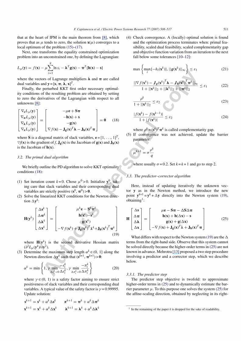
(4) Check convergence. A (locally) optimal solution is foundand the optimization process terminates when: primal fea-sibility, scaled dual feasibility, scaled complementarity gapand objective function variation from an iteration to the nextfall below some tolerances [10–12]:

max

{max

i{−hi(xk)}, ||g(xk)||∞

}≤ ε1 (21)

||∇f (xk)− Jg(xk)T

� − Jh(xk)T

�k||∞1+ ||xk||2 + ||�k||2 + ||�k||2

≤ ε1 (22)

ρk

1+ ||xk||2 ≤ ε2 (23)

|f (xk)− f (xk−1)|1+ |f (xk)| ≤ ε2 (24)

where ρk = (sk)T�k is called complementarity gap.(5) If convergence was not achieved, update the barrier

parameter:

μk+1 = σρk

q

where usually σ = 0.2. Set k = k + 1 and go to step 2.

3.3. The predictor–corrector algorithm

Here, instead of updating iteratively the unknown vec-tor y as in the Newton method, we introduce the newpoint yk+1 = yk + �y directly into the Newton system (19),obtaining1:

H

⎡⎢⎢⎢⎣

�s

��

��

�x

⎤⎥⎥⎥⎦ =

⎡⎢⎢⎢⎣

μe− S�−�S��

h(x)+ h(�x)− sg(x)+ g(�x)

−∇f (x)+ Jg(x)T λ+ Jh(x)T �

⎤⎥⎥⎥⎦ (25)

What differs with respect to the Newton system (19) are the �

terms from the right-hand side. Observe that this system cannotbe solved directly because the higher-order terms in (25) are notknown in advance. Mehrotra [13] proposed a two step procedureinvolving a predictor and a corrector step, which we describebelow.

3.3.1. The predictor stepThe predictor step objective is twofold: to approximate

higher-order terms in (25) and to dynamically estimate the bar-rier parameter μ. To this purpose one solves the system (25) forthe affine-scaling direction, obtained by neglecting in its right-

1 In the remaining of the paper k is dropped for the sake of readability.

Autho

r's

pers

onal

co

py

512 F. Capitanescu et al. / Electric Power Systems Research 77 (2007) 508–517

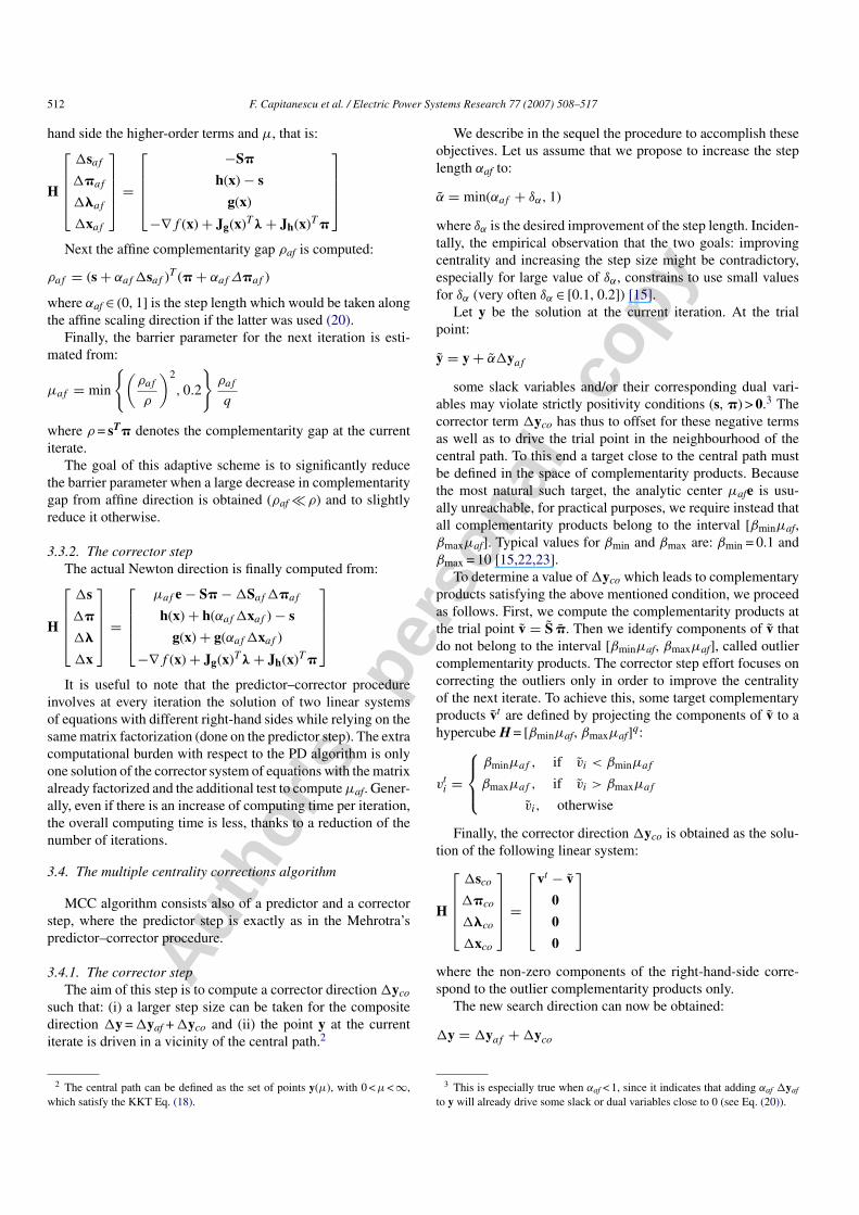
hand side the higher-order terms and μ, that is:

H

⎡⎢⎢⎢⎣

�saf

��af

��af

�xaf

⎤⎥⎥⎥⎦ =

⎡⎢⎢⎢⎣

−S�

h(x)− s

g(x)

−∇f (x)+ Jg(x)T λ+ Jh(x)T �

⎤⎥⎥⎥⎦

Next the affine complementarity gap ρaf is computed:

ρaf = (s+ αaf �saf )T (�+ αaf Δ�af )

where αaf ∈ (0, 1] is the step length which would be taken alongthe affine scaling direction if the latter was used (20).

Finally, the barrier parameter for the next iteration is esti-mated from:

μaf = min

{(ρaf

ρ

)2

, 0.2

}ρaf

q

where ρ = sT� denotes the complementarity gap at the currentiterate.

The goal of this adaptive scheme is to significantly reducethe barrier parameter when a large decrease in complementaritygap from affine direction is obtained (ρaf� ρ) and to slightlyreduce it otherwise.

3.3.2. The corrector stepThe actual Newton direction is finally computed from:

H

⎡⎢⎢⎢⎣

�s

��

��

�x

⎤⎥⎥⎥⎦ =

⎡⎢⎢⎢⎣

μaf e− S�−�Saf ��af

h(x)+ h(αaf �xaf )− s

g(x)+ g(αaf �xaf )

−∇f (x)+ Jg(x)T λ+ Jh(x)T �

⎤⎥⎥⎥⎦

It is useful to note that the predictor–corrector procedureinvolves at every iteration the solution of two linear systemsof equations with different right-hand sides while relying on thesame matrix factorization (done on the predictor step). The extracomputational burden with respect to the PD algorithm is onlyone solution of the corrector system of equations with the matrixalready factorized and the additional test to compute μaf. Gener-ally, even if there is an increase of computing time per iteration,the overall computing time is less, thanks to a reduction of thenumber of iterations.

3.4. The multiple centrality corrections algorithm

MCC algorithm consists also of a predictor and a correctorstep, where the predictor step is exactly as in the Mehrotra’spredictor–corrector procedure.

3.4.1. The corrector stepThe aim of this step is to compute a corrector direction �yco

such that: (i) a larger step size can be taken for the compositedirection �y = �yaf + �yco and (ii) the point y at the currentiterate is driven in a vicinity of the central path.2

2 The central path can be defined as the set of points y(μ), with 0 < μ <∞,which satisfy the KKT Eq. (18).

We describe in the sequel the procedure to accomplish theseobjectives. Let us assume that we propose to increase the steplength αaf to:

α = min(αaf + δα, 1)

where δα is the desired improvement of the step length. Inciden-tally, the empirical observation that the two goals: improvingcentrality and increasing the step size might be contradictory,especially for large value of δα, constrains to use small valuesfor δα (very often δα ∈ [0.1, 0.2]) [15].

Let y be the solution at the current iteration. At the trialpoint:

y = y+ α�yaf

some slack variables and/or their corresponding dual vari-ables may violate strictly positivity conditions (s, �) > 0.3 Thecorrector term �yco has thus to offset for these negative termsas well as to drive the trial point in the neighbourhood of thecentral path. To this end a target close to the central path mustbe defined in the space of complementarity products. Becausethe most natural such target, the analytic center μafe is usu-ally unreachable, for practical purposes, we require instead thatall complementarity products belong to the interval [βminμaf,βmaxμaf]. Typical values for βmin and βmax are: βmin = 0.1 andβmax = 10 [15,22,23].

To determine a value of �yco which leads to complementaryproducts satisfying the above mentioned condition, we proceedas follows. First, we compute the complementarity products atthe trial point v = S �. Then we identify components of v thatdo not belong to the interval [βminμaf, βmaxμaf], called outliercomplementarity products. The corrector step effort focuses oncorrecting the outliers only in order to improve the centralityof the next iterate. To achieve this, some target complementaryproducts vt are defined by projecting the components of v to ahypercube H = [βminμaf, βmaxμaf]q:

vti =

⎧⎪⎨⎪⎩

βminμaf , if vi < βminμaf

βmaxμaf , if vi > βmaxμaf

vi, otherwise

Finally, the corrector direction �yco is obtained as the solu-tion of the following linear system:

H

⎡⎢⎢⎢⎣

�sco

��co

��co

�xco

⎤⎥⎥⎥⎦ =

⎡⎢⎢⎢⎣

vt − v

0

0

0

⎤⎥⎥⎥⎦

where the non-zero components of the right-hand-side corre-spond to the outlier complementarity products only.

The new search direction can now be obtained:

�y = �yaf +�yco

3 This is especially true when αaf < 1, since it indicates that adding αaf �yaf

to y will already drive some slack or dual variables close to 0 (see Eq. (20)).

Autho

r's

pers

onal

co

py

F. Capitanescu et al. / Electric Power Systems Research 77 (2007) 508–517 513

Then, the actual step length α is computed so as to preservenon-negativity conditions and variables are updated:

y← y+ α�y

The corrector step can be applied several times. In such acase, the current direction �y becomes the predictor for a newcorrector, that is:

�yaf ← �yaf +�yco and αaf ← α

The computation of a new centrality correction terminatesas soon as one of the following conditions is achieved: (i) themaximal number of corrections allowed K is reached, (ii) thegain in step length (α−αaf) is insignificant and (iii) the steplength becomes α = 1.

3.4.2. Some implementation issues of the MCC algorithmTo lighten the presentation, we have considered a common

step length α for updating both primal and dual variables. Ourexperience showed, however, that the MCC algorithm behavesbetter when applying separate step lengths in primal and dualspaces.

As regards the choice of the desired improvement of the stepsize δα, two solutions are proposed: either the use of a constantvalue δα = 0.1 [15,23], or the use of an adaptive value accordingto the formula δα = (1−αaf)/K while imposing additionally thatδα ought not to be smaller than 0.1 or greater than 0.2 [23,22]. Inorder to reduce the number of centrality corrections computed atan iteration while aiming to obtain the largest increase in the stepsize we suggest to set δα = 0.2. We have found that this settingoffers better convergence performances in terms of CPU timeand number of iterations than the above mentioned proposals.We have not encountered any convergence trouble caused bythis “optimistic” setting.

In our implementation we compute a new centrality correc-tion only if it improves considerably the step lengths. To thisend, we allow the computation of a new centrality correctiononly if the gain in step length (α−αaf) is superior to εα = 0.03.Some other authors have suggested that a value for εα as smallas 0.01 may be accepted [15,23].

The most challenging problem of the MCC algorithm is thechoice of the maximal number of corrections allowed K, as theobjective is not only to reduce the number of iterations com-paratively to the PC algorithm but also to save some CPU time.To this respect some heuristics were proposed in the literature[15,23]. We instead determine K as follows. Assume a givenpower system and OPF variant. We first solve this OPF variantby progressively increasing the maximal number of correctionsallowed K (going from 1 to 10, for instance). Then we randomlyperturb (e.g. modifying generators active power, load consump-tions, topology, etc.) the initial operating point of the powersystem to be optimized and repeat the previous step a prede-fined number of times. Finally, results are gathered togetherand the value of K that led to the overall smallest CPU timeis determined. This value is automatically used for all subse-quent solutions of the same type of OPF variant and the samepower system. This procedure for choosing K proved to be quiterobust.

Note, finally, that the algorithms performance in terms ofCPU time may also depend somewhat on to the solver used forthe solution of the linear system of equations. In this work werely on the sparse object-oriented library SPOOLES [25]. Thislibrary, to the best of our knowledge, is not widely used butexhibits excellent performance of its linear algebra kernel (seealso Netlib web-site: www.netlib.org).

4. Numerical results

In this section we present numerical results of four OPFapplications while comparing PD, PC and MCC algorithms per-formance. The OPF has been coded in C++ and runs underCygwin or Linux environments. It has been tested on threetest systems, namely a 60 bus system which is a modifiedvariant of the Nordic32 system, and the popular IEEE118 andIEEE300 systems. A summary of these test systems is given inTable 1.

All tests have been performed on a PC Pentium IV of 1.7 GHzand 512 MB RAM. The MCC algorithm runs with the followingparameters: βmin = 0.1, βmax = 10, δα = 0.2 and εα = 0.03.

The convergence tolerances are set to ε1 = 10−4 for the primalfeasibility (21) and the scaled dual feasibility (22), and ε2 = 10−6

for the scaled complementarity gap (23) and the scaled objectivefunction variation from an iteration to the next (24).

4.1. Minimizing active power losses

We first deal with the minimization of transmission activepower losses (2), counted as the sum of active losses overall branches of the system. We consider the following con-trol variables: slack generator active power, generators reactivepower, controllable transformers ratio and shunt reactance. Theequality constraints involve the buses power balance (5) and(6). The inequality constraints concern bounds on: generatorsreactive power (11), voltage magnitudes (9), transformer withcontrollable ratio (12) and shunt reactance (13). Voltage mag-nitudes are allowed to vary between 0.95 pu and 1.05 pu in allbuses.

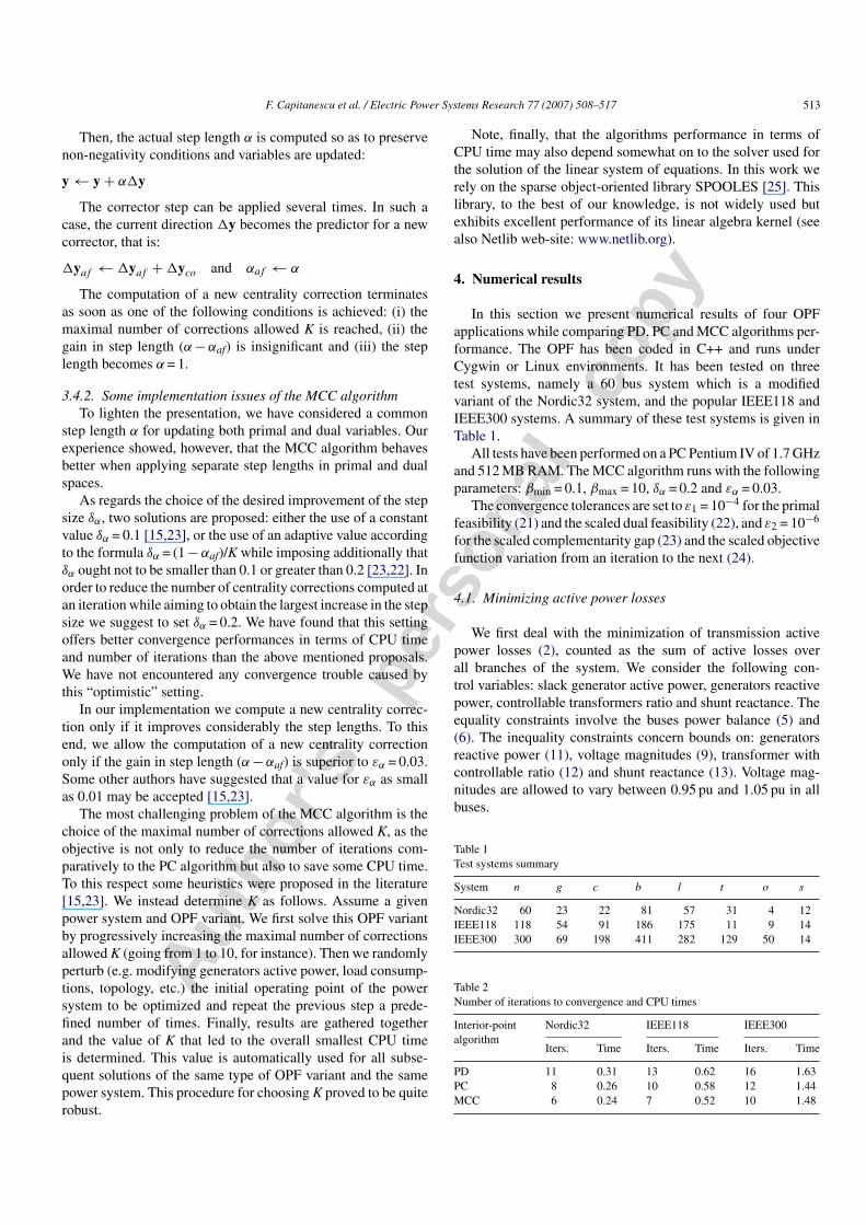
Table 1Test systems summary

System n g c b l t o s

Nordic32 60 23 22 81 57 31 4 12IEEE118 118 54 91 186 175 11 9 14IEEE300 300 69 198 411 282 129 50 14

Table 2Number of iterations to convergence and CPU times

Interior-pointalgorithm

Nordic32 IEEE118 IEEE300

Iters. Time Iters. Time Iters. Time

PD 11 0.31 13 0.62 16 1.63PC 8 0.26 10 0.58 12 1.44MCC 6 0.24 7 0.52 10 1.48

Autho

r's

pers

onal

co

py

514 F. Capitanescu et al. / Electric Power Systems Research 77 (2007) 508–517

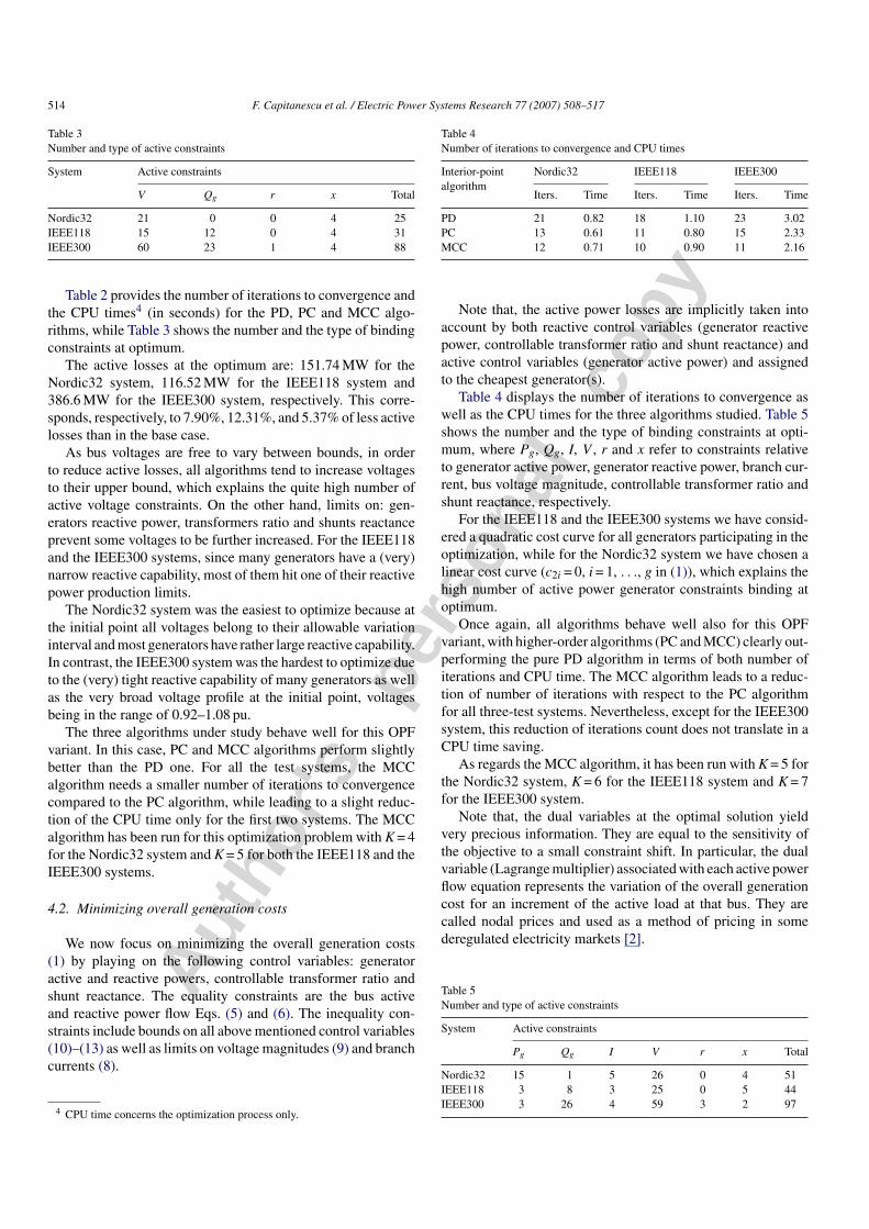
Table 3Number and type of active constraints

System Active constraints

V Qg r x Total

Nordic32 21 0 0 4 25IEEE118 15 12 0 4 31IEEE300 60 23 1 4 88

Table 2 provides the number of iterations to convergence andthe CPU times4 (in seconds) for the PD, PC and MCC algo-rithms, while Table 3 shows the number and the type of bindingconstraints at optimum.

The active losses at the optimum are: 151.74 MW for theNordic32 system, 116.52 MW for the IEEE118 system and386.6 MW for the IEEE300 system, respectively. This corre-sponds, respectively, to 7.90%, 12.31%, and 5.37% of less activelosses than in the base case.

As bus voltages are free to vary between bounds, in orderto reduce active losses, all algorithms tend to increase voltagesto their upper bound, which explains the quite high number ofactive voltage constraints. On the other hand, limits on: gen-erators reactive power, transformers ratio and shunts reactanceprevent some voltages to be further increased. For the IEEE118and the IEEE300 systems, since many generators have a (very)narrow reactive capability, most of them hit one of their reactivepower production limits.

The Nordic32 system was the easiest to optimize because atthe initial point all voltages belong to their allowable variationinterval and most generators have rather large reactive capability.In contrast, the IEEE300 system was the hardest to optimize dueto the (very) tight reactive capability of many generators as wellas the very broad voltage profile at the initial point, voltagesbeing in the range of 0.92–1.08 pu.

The three algorithms under study behave well for this OPFvariant. In this case, PC and MCC algorithms perform slightlybetter than the PD one. For all the test systems, the MCCalgorithm needs a smaller number of iterations to convergencecompared to the PC algorithm, while leading to a slight reduc-tion of the CPU time only for the first two systems. The MCCalgorithm has been run for this optimization problem with K = 4for the Nordic32 system and K = 5 for both the IEEE118 and theIEEE300 systems.

4.2. Minimizing overall generation costs

We now focus on minimizing the overall generation costs(1) by playing on the following control variables: generatoractive and reactive powers, controllable transformer ratio andshunt reactance. The equality constraints are the bus activeand reactive power flow Eqs. (5) and (6). The inequality con-straints include bounds on all above mentioned control variables(10)–(13) as well as limits on voltage magnitudes (9) and branchcurrents (8).

4 CPU time concerns the optimization process only.

Table 4Number of iterations to convergence and CPU times

Interior-pointalgorithm

Nordic32 IEEE118 IEEE300

Iters. Time Iters. Time Iters. Time

PD 21 0.82 18 1.10 23 3.02PC 13 0.61 11 0.80 15 2.33MCC 12 0.71 10 0.90 11 2.16

Note that, the active power losses are implicitly taken intoaccount by both reactive control variables (generator reactivepower, controllable transformer ratio and shunt reactance) andactive control variables (generator active power) and assignedto the cheapest generator(s).

Table 4 displays the number of iterations to convergence aswell as the CPU times for the three algorithms studied. Table 5shows the number and the type of binding constraints at opti-mum, where Pg, Qg, I, V , r and x refer to constraints relativeto generator active power, generator reactive power, branch cur-rent, bus voltage magnitude, controllable transformer ratio andshunt reactance, respectively.

For the IEEE118 and the IEEE300 systems we have consid-ered a quadratic cost curve for all generators participating in theoptimization, while for the Nordic32 system we have chosen alinear cost curve (c2i = 0, i = 1, . . ., g in (1)), which explains thehigh number of active power generator constraints binding atoptimum.

Once again, all algorithms behave well also for this OPFvariant, with higher-order algorithms (PC and MCC) clearly out-performing the pure PD algorithm in terms of both number ofiterations and CPU time. The MCC algorithm leads to a reduc-tion of number of iterations with respect to the PC algorithmfor all three-test systems. Nevertheless, except for the IEEE300system, this reduction of iterations count does not translate in aCPU time saving.

As regards the MCC algorithm, it has been run with K = 5 forthe Nordic32 system, K = 6 for the IEEE118 system and K = 7for the IEEE300 system.

Note that, the dual variables at the optimal solution yieldvery precious information. They are equal to the sensitivity ofthe objective to a small constraint shift. In particular, the dualvariable (Lagrange multiplier) associated with each active powerflow equation represents the variation of the overall generationcost for an increment of the active load at that bus. They arecalled nodal prices and used as a method of pricing in somederegulated electricity markets [2].

Table 5Number and type of active constraints

System Active constraints

Pg Qg I V r x Total

Nordic32 15 1 5 26 0 4 51IEEE118 3 8 3 25 0 5 44IEEE300 3 26 4 59 3 2 97

Autho

r's

pers

onal

co

py

F. Capitanescu et al. / Electric Power Systems Research 77 (2007) 508–517 515

Table 6Number of iterations to convergence and CPU times

Interior-pointalgorithm

Nordic32 IEEE118 IEEE300

Iters. Time Iters. Time Iters. Time

PD 19 0.48 21 0.99 47 4.65PC 11 0.37 15 0.83 19 2.60MCC 9 0.33 11 0.78 14 2.46

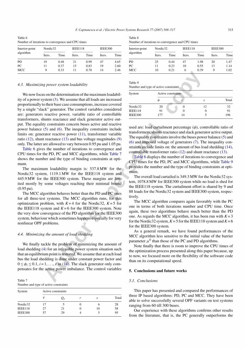
4.3. Maximizing power system loadability

We now focus on the determination of the maximum loadabil-ity of a power system (3). We assume that all loads are increasedproportionally to their base case consumptions, increase coveredby a single “slack” generator. The control variables consideredare: generators reactive power, variable ratio of controllabletransformers, shunts reactance and slack generator active out-put. The equality constraints concern buses active and reactivepower balance (5) and (6). The inequality constraints includelimits on: generator reactive power (11), transformer variableratio (12), shunt reactance (13) and bus voltage magnitudes (9)only. The latter are allowed to vary between 0.95 pu and 1.05 pu.

Table 6 gives the number of iterations to convergence andCPU times for the PD, PC and MCC algorithms, while Table 7shows the number and the type of binding constraints at opti-mum.

The maximum loadability margin is: 537.8 MW for theNordic32 system, 1119.1 MW for the IEEE118 system and445.9 MW for the IEEE300 system. These margins are lim-ited mostly by some voltages reaching their minimal bound(0.95 pu).

The MCC algorithm behaves better than the PD and PC onesfor all three-test systems. The MCC algorithm runs, for thisoptimization problem, with K = 4 for the Nordic32, K = 5 forthe IEEE118 system and K = 6 for the IEEE300 system. Notethe very slow convergence of the PD algorithm for the IEEE300system, behaviour which sometimes happens especially for verynonlinear OPF problems.

4.4. Minimizing the amount of load shedding

We finally tackle the problem of minimizing the amount ofload shedding (4) for an infeasible power system situation suchthat an equilibrium point is restored. We assume that at each loadbus the load shedding is done under constant power factor and0≤φi≤ 0.1, i = 1, . . ., c in (14). The slack generator only com-pensates for the active power imbalance. The control variables

Table 7Number and type of active constraints

System Active constraints

V Qg r x Total

Nordic32 17 5 0 6 28IEEE118 27 21 0 10 58IEEE300 57 29 4 5 95

Table 8Number of iterations to convergence and CPU times

Interior-pointalgorithm

Nordic32 IEEE118 IEEE300

Iters. Time Iters. Time Iters. Time

PD 25 0.44 47 1.98 20 1.47PC 11 0.23 10 0.55 13 1.14MCC 10 0.21 6 0.39 9 1.02

Table 9Number and type of active constraints

System Active constraints

φ r x Total

Nordic32 20 0 12 32IEEE118 91 0 0 91IEEE300 177 14 5 196

used are: load curtailment percentage (φ), controllable ratio oftransformers, shunts reactance and slack generator active output.The equality constraints involve the buses power balance (5) and(6) and imposed voltage of generators (7). The inequality con-straints include limits on: the amount of bus load shedding (14),controllable transformer ratio (12) and shunt reactance (13).

Table 8 displays the number of iterations to convergence andCPU times for the PD, PC and MCC algorithms, while Table 9provides the number and the type of binding constraints at opti-mum.

The overall load curtailed is 349.3 MW for the Nordic32 sys-tem, 1078.8 MW for IEEE300 system while no load is shed forthe IEEE118 system. The curtailment effort is shared by 9 and88 loads for the Nordic32 system and IEEE300 system, respec-tively.

The MCC algorithm compares again favorably with the PCone in terms of both iterations number and CPU time. Onceagain, these two algorithms behave much better than the PDone. As regards the MCC algorithm, it has been run with K = 3for the Nordic32 system, K = 5 for the IEEE118 system and K = 6for the IEEE300 system.

As a general remark, we have found performances of theMCC algorithm less sensitive to the initial value of the barrierparameter μ0 than those of the PC and PD algorithms.

Note finally that there is room to improve the CPU times ofthe optimization process presented along this paper because, upto now, we focused more on the flexibility of the software codethan on its computational speed.

5. Conclusions and future works

5.1. Conclusions

This paper has presented and compared the performances ofthree IP based algorithms: PD, PC and MCC. They have beenable to solve successfully several OPF variants on test systemsranging from 60 till 300 buses.

Our experience with these algorithms confirms other resultsfrom the literature, that is, the PC generally outperforms the

Autho

r's

pers

onal

co

py

516 F. Capitanescu et al. / Electric Power Systems Research 77 (2007) 508–517

PD algorithm in terms of CPU time, and thereby number ofiterations, on large-scale optimization problems. The oppo-site situation sometimes happens, especially for rather simpleproblems.

The results obtained suggest also that the MCC algorithm isa highly viable alternative to the successful PC algorithm. Thegood performances of the MCC algorithm emphasize once morethe importance of keeping the current iterate along the centralpath.

5.2. Future works

As regards the MCC algorithm, future work aims to find abetter heuristic scheme to automatically choose the maximumnumber of corrections allowed K for a given problem, in as muchas the best value of K shifts from an OPF variant to another andfrom a test system to another.

A natural extension of this work is the development of ahybrid algorithm, in which the corrector step combines bothMCC and PC features, in order to take advantage of their respec-tive qualities, as reported in [22].

A challenging future work is the development of a secu-rity constrained OPF (SCOPF), which handles together basecase constraints and steady-state security constraints relative tocredible (mainly “N− 1”) contingencies [28]. The benchmarkSCOPF is stated as an extension of the base case OPF model(1)–(14) that includes a set of equality and inequality constraintsof type (5)–(14) for each post-contingency state. One may dis-tinguish between two SCOPF formulations: “preventive” and“corrective”. The difference between these variants is that, inthe preventive SCOPF, the re-scheduling of control variables inpost-contingency states is not allowed. The major drawback ofthe brute force approach to the SCOPF benchmark is the highdimensionality of the problem, especially for large power sys-tems and many contingent cases.

Since not all contingencies constrain the optimum, clearly,there is a need to filter out such “harmless” contingencies andto perform the SCOPF with “harmful” contingencies only. Thesimplest technique for contingency filtering is post-contingencyconstraint relaxation. Thus, one first runs the SCOPF with thebase case constraints only. Then, at the resulted optimal solu-tion, contingencies are simulated one by one. If no contingencyviolates any security limit the solution is found, otherwise theequality and inequality constraints relative to those contingen-cies which violate some limits or are very close to them areadded to the SCOPF.

A widely used common approach to both SCOPF variantsconsists in adding to the base case constraints only relevantpost-contingency inequalities, linearized around the base caseoptimized operating point, while dropping all post-contingencyequality constraints. The latter constraints are however checkedat the optimal solution. This approach requires iterating betweenthe solution of the SCOPF and the linearization of post-contingency inequality constraints until some convergence cri-teria are met.

Alternatively, Benders decomposition is a very promisingtechnique to deal with a corrective SCOPF [29]. In this approach

the original SCOPF problem is decomposed into a master prob-lem and some slave problems, each corresponding to a harmfulcontingency case. Thus, a slave problem encompasses mainlythe post-contingency constraints relative to a contingency andprovides a linear constraint (Benders cut) to the master problem.The latter contains base case constraints and Benders cuts stem-ming from slave problems. At each iteration the slave problemsfed the master problem with improved Benders cuts until con-vergence is reached. Clearly, the simultaneous solution of slaveproblems, distributed among several processors, is possible; itcan significantly speed-up computations.

Besides, finding a trade-off between both preventive and cor-rective SCOPF variants still remains an open question [30].

Acknowledgments

This work is funded by the “Region Wallonne” in the frame-work of the project PIGAL (French acronym for Interior PointGenetic ALgorithm), RW 215187. Damien Ernst acknowledgesthe financial support of the Belgian National Fund of Scien-tific Research (FNRS) of which he is a post-doctoral ResearchFellow.

References

[1] J. Carpentier, Contribution a l’etude du dispatching economique, Bulletinde la Societe Franchise d’Electricite 3 (1962) 431–447.

[2] R.D. Christie, B.F. Wollenberg, I. Wangensteen, Transmission managementin the deregulated environment, IEEE Proc. 88 (2000) 170–195.

[3] H.W. Dommel, W.F. Tinney, Optimal power flow solutions, IEEE Trans.Power Ap. Syst. PAS-87 (10) (1968) 1866–1876.

[4] G.F. Reid, L. Hasdorf, Economic dispatch using quadratic programming,IEEE Trans. Power Ap. Syst. PAS-92 (1973) 2015–2023.

[5] B. Stott, E. Hobson, Power system security control calculation using linearprogramming, IEEE Trans. Power Ap. Syst. PAS-97 (5) (1978) 1713–1731.

[6] D.I. Sun, B. Ashley, B. Brewer, A. Hughes, W.F. Tinney, Optimal powerflow by newton approach, IEEE Trans. Power Ap. Syst. PAS-103 (10)(1984) 2864–2880.

[7] K.R. Frisch, The Logarithmic Potential Method of Convex Programming,Manuscript at Institute of Economics, University of Oslo, Norway, 1955.

[8] A.V. Fiacco, G.P. McCormick, Nonlinear Programming: Sequential Uncon-strained Minimization Techniques, John Willey and Sons, 1968.

[9] Y.C. Wu, A.S. Debs, R.E. Marsten, A direct nonlinear predictor–corrector primal-dual interior point algorithm for optimal power flows,IEEE Trans. Power Syst. 9 (2) (1994) 876–883.

[10] S. Granville, Optimal reactive dispatch through interior point methods,IEEE Trans. Power Syst. 9 (1) (1994) 136–142.

[11] G.D. Irrisari, X. Wang, J. Tong, S. Mokhtari, Maximum loadability of powersystems using interior point nonlinear optimization methods, IEEE Trans.Power Syst. 12 (1) (1997) 162–172.

[12] G.L. Torres, V.H. Quintana, An interior-point method for nonlinear optimalpower flow using rectangular coordinates, IEEE Trans. Power Syst. 13 (4)(1998) 1211–1218.

[13] S. Mehrotra, On the implementation of a primal-dual interior point method,SIAM J. Optim. 2 (1992) 575–601.

[14] T.J. Carpenter, I.J. Lusting, J.M. Mulvey, D.F. Shanno, Higher-orderpredictor–corrector interior point methods with application to quadraticobjectives, SIAM J. Optim. 3 (1993) 696–725.

[15] J. Gondzio, Multiple centrality corrections in a primal-dual method forlinear programming, Comput. Optim. Appl. 6 (1996) 137–156.

[16] G. Tognola, R. Bacher, Unlimited point algorithm for OPF problems, IEEETrans. Power Syst. 14 (3) (1999) 1046–1054.

Autho

r's

pers

onal

co

py

F. Capitanescu et al. / Electric Power Systems Research 77 (2007) 508–517 517

[17] G.L. Torres, V.H. Quintana, Optimal power flow by a nonlinear comple-mentarity method, IEEE Trans. Power Syst. 15 (3) (2000) 1028–1033.

[18] G.L. Torres, V.H. Quintana, A Jacobian smoothing nonlinear complemen-tarity method for solving optimal power flows, in: PSCC Conference,Sevilla, Spain, 2002.

[19] F. Capitanescu, M. Glavic, L. Wehenkel, An interior-point method basedoptimal power flow, in: ACOMEN Conference, Ghent, Belgium, June,2005, p. 18.

[20] F. Capitanescu, M. Glavic, L. Wehenkel, Applications of an interior-pointmethod based optimal power flow, in: CEE Conference, Coimbra, Portugal,October, 2005, p. 6.

[21] F. Capitanescu, M. Glavic, L. Wehenkel, Experience with the multiplecentrality corrections interior-point algorithm for optimal power flow, in:CEE Conference, Coimbra, Portugal, October, 2005, p. 6.

[22] M.J. Rider, C.A. Castro, M.F. Bedrinana, A.V. Garcia, Towards a fast androbust interior point method for power system applications, IEE Proc.Gener. Transm. Distribut. 151 (2004) 575–581.

[23] G.L. Torres, V.H. Quintana, On a nonlinear multiple centrality correctionsinterior-point method for optimal power flow, IEEE Trans. Power Syst. 16(2) (2001) 222–228.

[24] H. Wei, H. Sasaki, J. Kubokawa, R. Yokohama, An interior point nonlinearprogramming for optimal power flow with a novel data structure, IEEETrans. Power Syst. 13 (3) (1998) 870–877.

[25] C. Ashcraft, R. Grimes, SPOOLES: an object-oriented sparse matrixlibrary, in: Proceedings of the 1999 SIAM Conference on Parallel Pro-cessing for Scientific Computing, 1999, pp. 22–27.

[26] G.L. Torres, Nonlinear Optimal Power Flow by Interior and Non-interiorPoint Methods, PhD Thesis, University of Waterloo, Canada, 1998.

[27] J.L. Martinez Ramos, A. Gomez Exposito, V.H. Quintana, Transmissionpower loss reduction by interior-point methods: implementation issues andpractical experience, IEE Proc. Gener. Transm. Distribut. 152 (1) (2005)90–98.

[28] O. Alsac, B. Stott, Optimal load flow with steady-state security, IEEE Trans.Power Ap. Syst. PAS-93 (3) (1974) 745–751.

[29] R.A. Schlueter, S. Liu, N. Alemadi, Preventive and corrective open accesssystem dispatch based on the voltage stability security assessment anddiagnosis, Electr. Power Syst. Res. 60 (2001) 17–28.

[30] J. Carpentier, D. Menniti, A. Pinnarelli, N. Scordino, N. Sorrentino, Amodel for the ISO insecurity costs management in a deregulated marketscenario, in: IEEE Power Tech. Conference, Porto, September, 2001.