Inter-instrument comparison of particle-size analysers1

Sam Robersona,∗, Gert Jan Weltjeb2

aGeological Survey of Northern Ireland, Colby House, Stranmillis Court, Belfast, BT9 5BF, United Kingdom.3bDelft University of Technology, Faculty of Civil Engineering and Geoscience, Department of Geoscience and Engineering, Stevinweg 1, Delft 26284

CN, The Netherlands5

Abstract6

This paper presents a methodological framework for inter-instrument comparison of different particle-size analysers.7

The framework consists of: (i) quantifying the difference between complete particle-size distributions, (ii) identifying the8

best regression model for homogenising data sets of particle-size distributions measured by different instruments, (iii)9

quantifying the precision of a range of particle-size analysers, and (iv) identifying the most appropriate instrument for10

analysing a given set of samples. The log-ratio transform is applied to particle-size distributions throughout this study11

to avoid the pitfalls of analysing percentage-frequency data in ‘closed-space’. A Normalized Distance statistic is used12

to quantify the difference between particle-size distributions and assess the performance of logratio regression models.13

Forty-six different regression models are applied to sediment samples measured by both sieve-pipette and laser analysis.14

Interactive quadratic regression models offer the best means of homogenising data sets of particle-size distributions15

measured by different instruments into a comparable format. However, quadratic interactive logratio regression models16

require a large number of training samples (n > 80) to achieve optimal performance compared to linear regression17

models (n = 50). The precision of ten particle-size analysis instruments was assessed using a data set of ten replicate18

measurements made of four previously published silty sediment samples. Instrument precision is quantified as the19

median Normalised Difference measured between the ten replicate measurements made for each sediment sample. The20

Differentiation Power statistic is introduced to assess the ability of each instrument to detect differences between the four21

sediment samples. Differentiation Power scores show that instruments based on laser diffraction principles are able to22

differentiate most effectively between the samples of silty sediment at a 95% confidence level. Instruments applying the23

principles of sedimentation offer the next most precise approach.24

Keywords: analytical precision, differentiation power, particle-size distribution, laser diffraction, log-ratio analysis25

∗Corresponding authorEmail address: samrob@bgs.ac.uk (Sam Roberson)

Preprint submitted to Sedimentology November 10, 2013

PREPRINT

INTRODUCTION1

This paper presents a methodological framework for the inter-comparison of particle-size analysis instruments. The2

aims of this paper are to provide solutions to the following interconnected issues:3

i. Quantifying the difference between complete particle-size distributions4

ii. Adjusting for differences measured between particle-size distributions analysed by different instruments5

iii. Quantifying the precision of different particle-size analysers6

iv. Objectively identifying the most appropriate instrument for a given set of sediment samples7

The methods used by this study explicitly acknowledge the limitations of analysing percentage frequency data8

using traditional multivariate statistical techniques. An alternative approach is offered by a suite of techniques known9

collectively as ‘compositional data analysis’. Compositional data analysis has been applied to particle-size data for over10

thirty years, yet remains a comparatively unknown approach within the field of sedimentology (Aitchison, 1982, 1986,11

1999, 2003; von Eynatten, 2004; Weltje and Prins, 2003; Jonkers et al., 2009; Tolosana-Delgado and von Eynatten, 2009,12

2010; Weltje and Roberson, 2012). Many other examples of compositional data analysis exist in geoscience, including:13

mineral compositions of rocks (Thomas and Aitchison, 2006; Weltje, 2002, 2006), pollutant profiles (Howel, 2007), pollen14

populations (Jackson, 1997) and trace element compositions (von Eynatten et al., 2003). Initially it is helpful to provides a15

brief introduction to compositional data analysis and its relevance to inter-instrument comparison of particle-size analysers16

using a short example.17

The mathematical properties of particle-size distributions18

To appreciate the best way to analyse particle-size distributions, expressed as discrete particle-size percentage values,19

it is necessary to highlight some of their fundamental (often obvious) mathematical properties.20

1. Particle-size distributions contain relative information about the proportions of different particle-sizes in a sediment21

sample22

2. Particle-size categories are expressed as percentages, so are greater or equal to zero and less then or equal to 100%23

3. Particle-size distributions sum to 100%24

These properties are very useful in that they normalise measurements of particle mass or particle volume, allowing25

for widespread data comparison. However, they also represent serious obstacles to multivariate statistical analysis and26

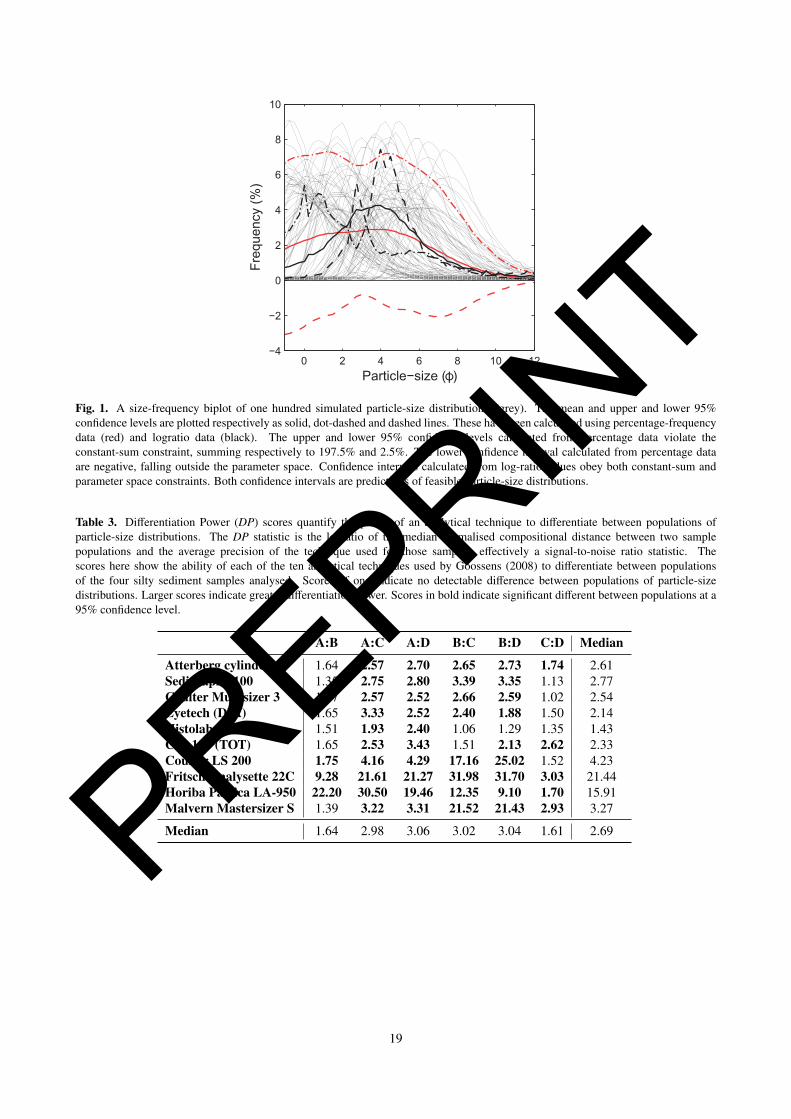
subsequent data interpretation. A data set of one hundred simulated size-frequency distributions is presented as (i) a27

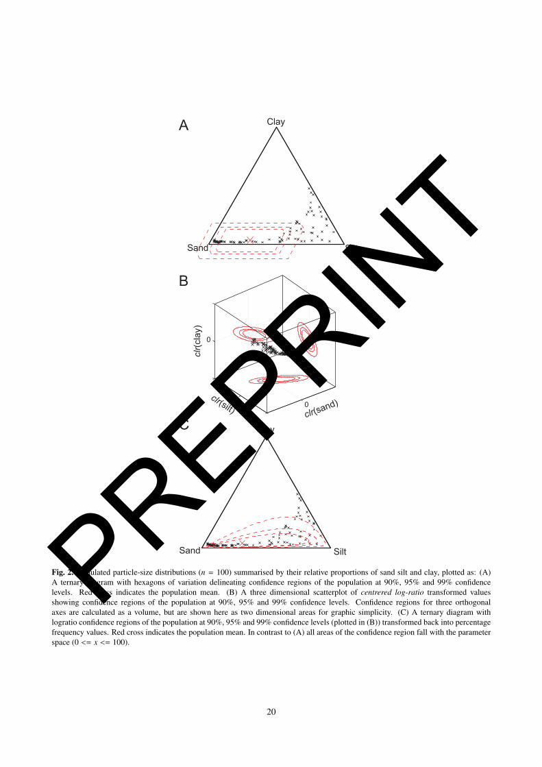
percentage-frequency plot (Fig. 1), and (ii) ternary diagrams (Fig. 2A, C). These data are used below to illustrate28

these mathematical properties act as constraints, limiting the extent to which standard statistical tests can be applied29

to particle-size distributions.30

The first constraint is that each part of a particle-size distribution must be considered in relation to all its other31

parts. This is because a change in one part of a distribution automatically results in an inverse change in all the other32

2

PREPRINT

parts of the distribution. For example, if there is an absolute increase in the mass of silt in a sample compared to1

another sample, the relative proportions of sand and clay will decrease, even if the mass of both of these size fractions2

remains constant. The lengthy description of the relative proportions of each part of a particle-size distribution can be3

avoided if log-normal distribution coefficients are used instead (Folk and Ward, 1957; Inman, 1952; Evans and Benn,4

2004). Comparisons between particle-size distributions are most commonly quantified using mean, standard deviation,5

skewness and kurtosis statistics. The limitations of this approach have been documented by several authors (Bagnold6

and Barndorff-Nielsen, 1980; Fredlund et al., 2000; Fieller et al., 1992; Beierle et al., 2002; Friedman, 1962), the most7

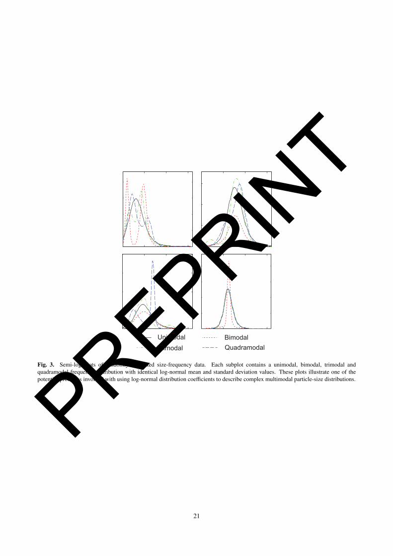
fundamental of which being that particle-size distributions are frequently not log-normal. Figure 3 illustrates how a series8

of markedly different multimodal distributions can have identical log-normal distribution coefficients (mean and standard9

deviation). Quantifying the analytical precision of an instrument is clearly problematic if the statistics used are unable to10

differentiate between particle-size distributions that are evidently dissimilar. Alternative probability distribution functions11

(e.g. log-hyperbolic, skew-Laplace) have been suggested to circumvent this issue (Bagnold and Barndorff-Nielsen,12

1980; Fieller et al., 1992), but the limitations of non-uniqueness are still applicable. Moreover, all distribution function13

statistics mask potentially important variations in empirical data. One means of avoiding the pitfalls of distribution14

function statistics has been to compare complete particle-size distributions using factor analysis (Syvitski, 1991; Stauble15

and Cialone, 1996). Unfortunately, in most cases this approach is not valid because percentage values in particle-size16

distributions are subject to bias (Falco et al., 2003). The source of this bias is detailed by the second constraint acting on17

particle-size distributions and is detailed below.18

The second constraint is that percentage frequency data occupy a mathematically limited space, 0 < x < 100. This19

has important implications for applying regression models to particle-size distributions, used for example when making20

adjustments to homogenise data sets analysed by a range of different instruments (Konert and Vandenberghe, 1997;21

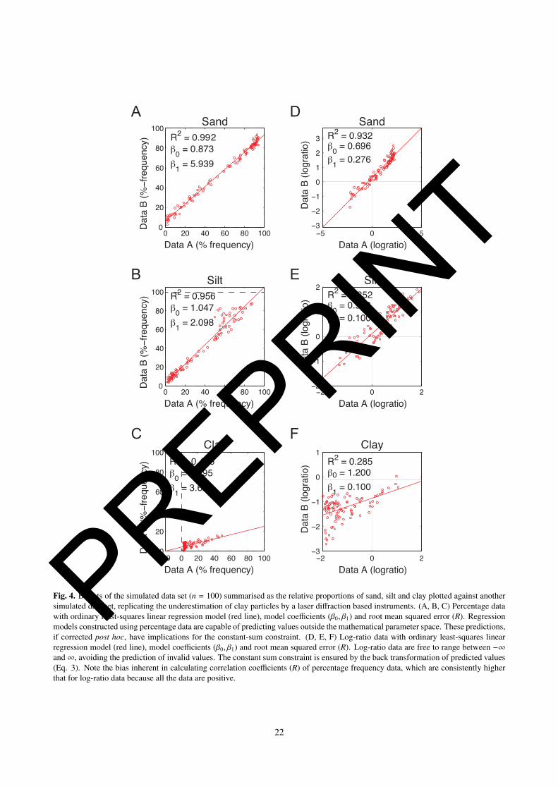
Beuselinck et al., 1998; Buurman et al., 2001; Eshel et al., 2004). Figure 4A, B, and C show the simulated data set (‘Data22

A’) of percentage frequency values plotted against another synthetic data set (‘Data B’) . Data set ‘B’ has been simulated23

to replicate the underestimation of clay particles by a laser diffraction instrument. A least-squares linear regression model24

has been calculated for each size fraction (solid red line) with model coefficients and R2 correlation coefficients given for25

each. R2 statistics are close to one for both sand and silt, indicating a good agreement between the two data sets. Close26

inspection of the regression models reveal that for the silt fraction (Fig. 4B) percentage values greater than one hundred27

are predicted for a the upper range of data, indicated by the horizontal dashed line. The inverse case is also true for the28

clay fraction (Fig. 4C), where the regression model predicts negative percentage values for data set A.29

Calculating confidence regions around populations of particle-size distributions is important if differences between30

populations are to be reliably determined. Confidence regions for ternary diagrams have traditionally been calculated31

using hexagonal fields of variation (Stevens et al., 1956; Weltje, 2002). These are plotted for the simulated data set in32

Figure 2 as confidence regions of the population at 90%, 95% and 99% confidence limits. Confidence intervals calculated33

using percentage frequency values have also been plotted in Figure 1. The red dashed line in Figure 1 indicates the lower34

3

PREPRINT

95th confidence limit of the population. In both the figures some of the values within the confidence regions fall outside1

the range of zero and one hundred, which is clearly impossible.2

The third constraint operating on particle-size distributions is that they must sum to one hundred. This restriction3

applies as equally to confidence intervals as it does to particle-size distributions modelled using regression functions. In4

the former case the upper and lower 95% confidence levels of the synthetic data calculated using percentage frequency5

values plotted in Figure 1 sum respectively to 197.5% and 2.5%. Were these estimates taken as correct they would violate6

principles of conservation of mass, implying that mass has the potential to both leave and enter the system. In the latter7

case, there is no way to guarantee that distributions predicted from percentage data will sum to one hundred. post hoc8

adjustments performed to ensure constant sum, unless done with extreme care, are liable to violate the first constraint by9

changing the relative proportions of the distribution.10

These three mathematical constraints impose serious limitations on how well particle-size data can be described and11

compared, and consequently the reliability with which the performance of particle-size analysers can be defined and12

compared.13

Compositional data14

To overcome the constraints detailed above, the principles of compositional data and the log-ratio transformation must15

be introduced. Data characterised mathematically as positive constant-sum vectors are known as compositional data16

(Aitchison, 1986). A single compositional data point is known as a composition, e.g. a particle-size distribution. Aitchison17

(1986) recognised that, because each part of a composition must be considered relative to all its other parts, they were best18

treated as ratios. Ratios are mathematically awkward, so Aitchison (1986) logically extended the transformation to derive19

the logarithm of the ratios, log-ratios. There are a number of different ways to calculate the log-ratio of compositions. For20

particle-size distributions composed of more than three parts the centered-log-ratio transform (clr) is generally the most21

useful:22

q = clr(p) =

[log

(pi

g(p)

). . . log

(pD

g(p)

)](1)

where q is the log-ratio transform of p, a particle-size distribution with D-particle-size categories, i is the ith category and23

g(p) is the geometric mean of the particle-size distribution p. For a three-part particle-size distribution [0.4 0.35 0.25] the24

log-ratio of the first category is:25

q1 = clr(p1) = log(

0.43√

0.4 ∗ 0.35 ∗ 0.25

)(2)

The log-ratio transformation of compositional data moves it from closed space to real space, also referred to as co-ordinate26

space. The transformation into co-ordinate space is best visualised by comparing Figure 2A to Figure 2B. In the latter27

three-dimensional scatterplot the log-ratios of the sand, silt and clay fractions are a dimension in co-ordinate space,28

4

PREPRINT

analogous to (x, y, z) Cartesian co-ordinates. In co-ordinate space where there are no parameter limits (data values range1

from −∞ to ∞) these data can be analysed using standard multivariate statistics without any of the restrictions described2

above.3

The application of linear regression models to particle-size distributions in co-ordinate space is illustrated by Figure4

4D, E and F. In co-ordinate space linear regression models are incapable of predicting ‘impossible’ values. Eq. 1 also5

removes the influence of bias on root mean squares error (RMSE) calculations because the data are both positive and6

negative. With the removal of this bias, correlation coefficients calculated using log-ratio data are notably lower than for7

the equivalent percentage frequency data in Figure 4A, B and C. Standard goodness-of-fit statistics can also be applied to8

data in co-ordinate space without the need to apply to moment measure statistics. The root mean squared error statistic9

applied in this case is identical to the Euclidian distance measurement normalised by degrees of freedom. This can be10

applied to compare the output of predictive models and instrument precision using replicate sample measurements.11

Working with log-ratio data allows population confidence regions to be predicted in a straightforward manner van den12

Boogaart and Tolosana-Delgado (2008). The red ellipses plotted in Figure 2B delineate confidence regions of the synthetic13

data population at 90%, 95% and 99% confidence limits. These are actually calculated as volumes using a trivariate14

probability model, but are plotted as orthogonal ellipses for graphical simplicity. To turn these confidence regions, along15

with modelled distributions, into meaningful information they must be converted back to percentage-frequency values.16

The transformation of log-ratio data back into constrained space is performed using the inverse log-ratio transform (clr−1):17

p∗ = clr−1(q) = [exp(qi)...exp(qD)] (3)

where qi is the ith part of a log-ratio particle-size distribution q. To arrive at percentage frequency values p∗ must be18

further adjusted using the closure operation C so that its component parts sum to 100%:19

p = p∗(

100sum(p∗)

)(4)

The inverted confidence intervals are plotted as a ternary diagram in Figure 2C and Figure 1. All the values within these20

confidence regions are conveniently within the parameter space and all sum to 100%. Modelled particle size distributions21

predicted using log-ratio regression models also obey closed-data restrictions following back transformation by Eq. 3.22

The example given above demonstrates how the log-ratio transformation (Eq. 1) can be used to overcome the23

restrictions of closed space and apply regression analysis and concepts of statistical confidence to comparing particle-size24

analysers.25

5

PREPRINT

METHODS1

The data sets2

This study makes use of an extensive database of high quality particle-size distributions (4837) collected and maintained3

by the Geological Survey of the Netherlands. Particle-size distributions were measured by Fritsch A22 XL (Fritsch4

GmbH, Idar-Oberstein, Germany) laser particle sizers at the University of Amsterdam (see supplementary Appendix A5

for details). A subset of 138 sediment samples from the database were re-analysed using traditional sieve-pipette methods6

(see supplementary Appendix B for details). The samples analysed were selected to be representative of the entire range7

of sedimentary environments in the Netherlands, i.e. marine, aeolian, fluvial and glacial.8

The issue of particle-size category mismatch between laser and sieve-pipette data was circumvented by amalgamating9

both data formats to a single uniform format composed of sixteen categories following Weltje and Roberson (2012). The10

amalgamated particle-size categories are at half-phi intervals for particles between -1 to 4 φ and at φ intervals for particles11

between 4 and 9 φ. These are the standard category intervals for sieve-pipette analysis. Included in the amalgamation12

process is a multiplicative zero-replacement strategy following Martın-Fernandez et al. (2003). This is an important step13

when working with log-ratio particle-size distributions, because zeros cannot be log transformed. The method used here14

ensures that zeros in the data are replaced by statistically realistic values (equivalent to machine accuracy), while also15

preserving the relative information contained in each distribution.16

Particle-size distributions published in a comparison study by Goossens (2008) are re-analysed by this study to quantify17

the relative precision and differentiation power of ten different instruments. The data set published by Goossens (2008)18

consists of four clayey silt sediment samples taken from Korbeek-Dijle, Belgium. Each sediment was measured ten19

times by ten different instruments, giving a total of 400 particle-size distributions. The data were extracted from20

cumulative-frequency particle-size distributions given in Goossens (2008, their Figure 11) by a digital image analysis21

algorithm. Particle-size categories from 3 to 14 φ at quarter φ intervals were used for these data. A high digitisation22

accuracy was achieved during by this process, primarily because the graphs were available in a vector format. To extract23

the data each individual cumulative-frequency curve was converted to a raster image (946 by 510 pixels). The images24

were registered using standard digital techniques, substituting the axis limits as (x,y) co-ordinates. Horizontal resolution25

was 0.11 µm for samples A and B and 0.08 µm for samples C and D. Vertical resolution was 0.2% for all samples.26

Prior to any analysis it was established using a Kolmogorov-Smirnov test for normality that none of the samples used in27

this study exhibited a log-normal distribution. This made comparison of distributions using a moment measures approach28

Inman (1952) unsuitable.29

Regression models30

The adjustment of sediment samples measured by both sieve-pipette and laser techniques were performed in31

co-ordinate-space using the clr transformation [Eq. 1]. Continuing with the notation introduced above q is given as the32

log-ratio of particle-size distributions p measured by sieve-pipette analysis and r the log-ratio of particle-size distributions33

6

PREPRINT

measured by laser analysis s. A range of multivariate regression models were used to model the relationship between q1

and r: linear, polynomial, quadratic and quadratic with interaction terms. Regression models were applied iteratively2

to each particle-size category to model the complete distribution. Polynomial and quadratic regression models were run3

using a range of two to sixteen terms, limited by the total number of particle-size categories available. Including the linear4

model, a total of forty-six different regression models were applied to particle-size calibration. The straightforward linear5

regression model is given in the familiar form:6

ri = qi ∗ β1 + β0 (5)

where ri is the ith particle-size category of the modelled distribution r, β0 is the intercept and β1 is slope. The second7

degree polynomial form is given as:8

ri = qi2 ∗ β2 + qi ∗ β1 + β0 (6)

where β1 and β2 are the first and second order model coefficients. The second order quadratic model without interaction9

is given as:10

ri = β4(qi−12) + β3(qi

2) + β2(qi−1) + β1(qi) + β0 (7)

where qi−1 is the particle-size category before qi and β4 and β3 are the coefficients for the squared terms. In the case where11

i = 1 the second term becomes q2. This rule was also applied to higher order models. The second-order quadratic model12

with interactive terms is given as:13

ri = β5(qi ∗ qi−1) + β4(qi−12) + β3(qi

2) + β2(qi−1) + β1(qi) + β0 (8)

where β5 is the coefficient of the interaction term qi ∗ qi−1. It is impractical to write out the formulae for all regression14

models used, so readers are directed to Devore (2011) for an up to date introduction to multivariate regression models.15

Goodness-of-fit statistics16

A normalised Euclidean distance statistic (ND) is used here to quantify the difference between log-ratio particle-size17

distributions a and b:18

ND(a,b) =1

D − 1·

√√√ D∑i=1

(ai − bi)2 (9)

where D is the number of particle size categories. Having defined a robust means of quantifying the difference between19

two particle-size distributions, it is now possible to apply the ND statistic to measuring: (i) the performance of the20

7

PREPRINT

regression models used for calibration; (ii) the precision of different analytical techniques; and (iii) the power with which1

an analytical technique can differentiate between two sediment samples.2

Model performance3

The performance of each regression model was assessed by calculating ND(r,r), the median ND between distributions4

measured by laser granulometry r and distributions predicted from sieve-pipette measurements r. In addition to calculating5

which model best fits the data using all the available samples, it is also pertinent to determine the influence of sample6

numbers on model performance. This was performed using a series of cross-validation tests. Cross validation tests7

involve partitioning a dataset into two subsets: a training set and a testing set. The training set is used to build the8

regression model, which is then tested by applying it to the testing set. The type of cross-validation applied here is9

known as k-fold cross-validation, where the data set is randomly partitioned into k subsamples and run k times. Random10

partitioning ensures that each iteration uses a different training set to create the model, which is then tested against all11

subsets, meaning that all data are eventually used for training and testing. To summarise model performance for ns/k12

training samples the ND statistic is averaged over all the results, where ns is the total number of samples in the dataset.13

A series of k-fold cross-validation tests were run for each of the forty-six regression models (linear, polynomial,14

quadratic and interactive quadratic). The tests were run for a range of training set sizes ns/k, from eight to one15

hundred and thirty eight at intervals of ten. To ensure that all combinations of training-testing portioning were used each16

cross-validation test was repeated 1000 times. The performance of each model for a given training set size was measured17

as the median ND statistic across the range of results. The results of these tests are a measure of model robustness and18

may be particularly important in determining which regression model should be used for any given set of samples.19

Analytical precision20

The precision of an analytical technique has been defined as the spread of repeat measurements around a central value,21

in this case precision is defined as the median ND score between all possible combinations of repeat measurements. The22

standard deviation of these ND statistics therefore quantifies how representative the median ND value is of technique23

precision, i.e. how well technique precision has been established.24

It should also be pointed out that with samples of natural sediment it is essentially impossible to determine the accuracy25

of a technique, because the actual size of particles is difficult to measure when they are in large numbers. Determining26

machine accuracy is therefore best attempted using standardised glass spheres in the manner of Konert and Vandenberghe27

(1997).28

Differentiation power29

The ability to quantify instrument precision raises some interesting questions. For example, if the precision of an30

instrument is low, at what point it still possible to reliably detect the difference between two populations of particle-size31

8

PREPRINT

distributions? Furthermore, if there is a measurable difference between the distributions, at what point is that difference1

significant?2

In order to answer these questions, the ND statistic is extended to calculate the power of an analytical technique to3

differentiate between sediment samples. The differentiation power DPT(a,b) of analytical technique T quantifies the ability4

of that technique to distinguish between two populations of particle-size distributions a and b. The DP statistic takes the5

form of a standard Z-score statistic, stating that if the distance between two populations is less than the spread of those6

populations then it is not possible to distinguish between them. DP is therefore defined as:7

DPT(a,b) =

ND(a,b)

s2p

(10)

where ND(a,b) is the median ND between all possible combinations of repeat measurements of sediment a and b, and S 2p8

is the pooled standard deviation. S 2p is defined as:9

√ND

2a · n + ND

2b · m

n + m − 2(11)

where NDa is the median ND score between all repeat measurements a. Eq 10 then is the log-ratio of the distance between10

two populations and the average precision of the technique used. n and m are respectively the sample size of populations11

a and b. This statistic has the same form as an independent two sample t-test (Davis, 2002), allowing significance to be12

assessed at a 95% confidence level for n + m − 2 degrees of freedom. Larger DP scores therefore correspond to a greater13

ability to distinguish between two groups of particle-size distributions. In such cases DP scores may be considered14

analogous to a high signal-to-noise ratio. DP scores of one mean that two populations of particle-size distributions are15

indistinguishable from each other.16

Note that the definition of technique precision given in the denominator of Eq. 10 is specific to each sediment, rather17

than the technique as a whole. This is an important distinction to make, given that particle shape and density in natural18

sediments may differ markedly between locations. Machine precision is then heavily dependant upon the particular shape19

and density of particles in the sediment measured.20

RESULTS AND DISCUSSION21

Predictive models22

This section presents the results of regression modelling applied to 138 Dutch particle-size distributions analysed by23

both sieve-pipette and laser diffraction. The specific results are therefore important only to geologists working with Dutch24

sediments that have been analysed by these two instruments. The wider aim here is to illustrate how the best regression25

model for any data set may be objectively identified using compositional data analysis.26

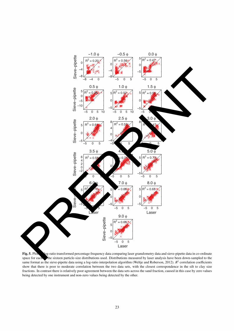
Figure 5 shows the sieve-pipette data plotted against laser data in co-ordinate space for all of the sixteen integrated27

particle-size categories. The basic correlation structure between the two data sets is quantified by a squared correlation28

9

PREPRINT

coefficient R2. The two data sets correspond most closely across the silt range (R2 > 0.7) and least closely for very coarse1

sands at -1 φ (R2 = 0.2) and coarse sands at 0.5 φ (R2 = 0.36). The comparatively high correlation between particles2

in the silt range is consistent with previous observations (Konert and Vandenberghe, 1997; Beuselinck et al., 1998) and3

is probably attributable to a relatively high proportion of near-spherical particles. The data structure of coarse-sand size4

particles in Figure 5 deviates considerably from the ideal 1:1 ratio (diagonal black line). Horizontal and vertical data5

clusters in these plots are caused by large proportions of particles being detected in a specific size range by one instrument6

which were not detected in the same size range by the other instrument. This discrepancy is likely to be caused by7

non-spherical particles in these size ranges (Beuselinck et al., 1998). Squared-mesh sieve stacks preferentially separate8

particles on the basis of the intermediate axis length, which can mask the presence of both elongated and bladed particles.9

Laser granulometry, in, contrast detects particles transported in a flowing medium using a diffraction algorithm, indicating10

that the long axes of elongated particles are more likely to be detected.11

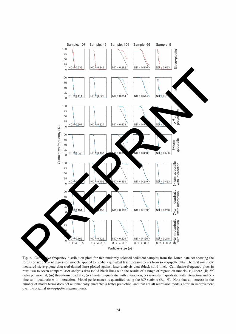
The results of predicting laser particle-size distributions from sieve-pipette data are shown in Figure 6 for five randomly12

selected samples. The first row of plots in Figure 6 compare cumulative frequency distributions for both laser and13

sieve-pipette data. Plots in rows two to six compare laser cumulative frequency distributions against modelled distributions14

for six of the forty-six regression models applied: linear, second-degree polynomial, three-term quadratic and five-,seven-15

and nine-term quadratic interaction models. The different regression models are highly variable in terms of how closely16

they fit the original laser data for individual particle-size distributions. No single model guarantees a better prediction17

for any one sample. For example, predictions for samples 45 and 66 (Fig. 6) is best achieved using a 9-term interactive18

quadratic model. In contrast, the five-term quadratic model for sample 107 has a higher ND score than the sieve-pipette19

measurement, 0.351 and 0.282 respectively.20

The tendency for regression models to not always generate an improved fit to the data reflects the fact that the difference21

between laser and sedimentation methods is not a linear problem, but a function of both three-dimensional particle shape22

and the density of individual sediment grains. Approaching this problem with a physically-based model that would enable23

complete conversion between two instruments based on different physical principles requires knowledge of both particle24

density and shape. An underlying issue in particle-size analysis therefore remains : our knowledge of particle-size remains25

incomplete in all but the most simple of cases.26

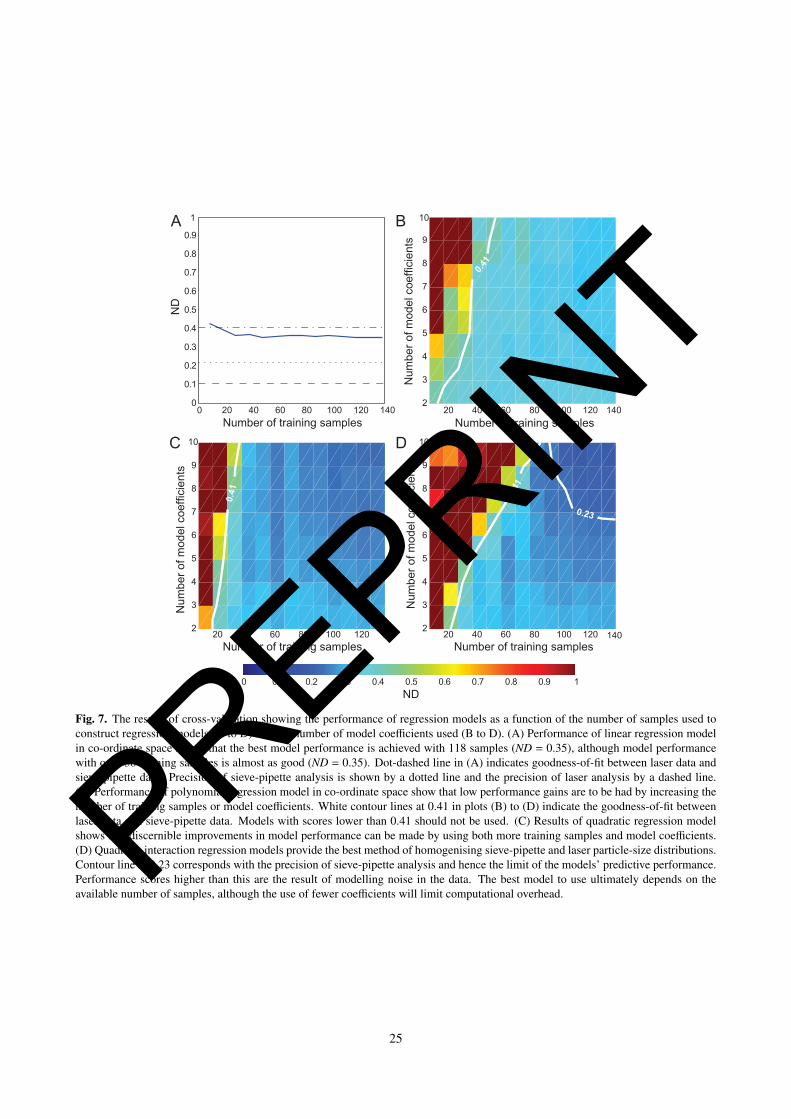
The performance of all regression models with respect to the number of samples used is summarised in Figure 7. For27

each type of model, both an increase in the number of training samples and coefficients used resulted in an increase28

in model performance. While this is not surprising, the results quantify for the first time the added value of using29

quadratic regression models over linear models for adjusting particle-size distributions measured by different techniques.30

Importantly, the results of the cross-validation analysis indicate which model is most suitable for the number of samples31

available. Models with ND scores higher than 0.41 (green-yellow-brown colours) should not be used because they do32

not predict better fit distributions than the original sieve-pipette data. Quadratic interaction models naturally require the33

largest number of samples to function adequately owing to the interaction terms, resulting in the best performance scores.34

10

PREPRINT

For models with seven or more coefficients, predictions made using all the available samples produced ND scores better1

than the precision of the sieve-pipette data (0.23). Given that model performance must be limited by the precision of the2

input data, this must therefore be the result of modelling noise in the data set. Any further improvements to modelling3

laser data may therefore only be achieved by acquiring higher precision sieve-pipette data. Taking into account the high4

levels of laboratory personnel experience, it is difficult to see how this could be achieved.5

On the basis of the cross-validation results presented in Figure 7, it is recommended that procedures adjusting for6

differences between laser and sieve-pipette data use a minimum of thirty replicate samples, and apply a two-term quadratic7

regression model. If more resources are available using at least ninety replicate samples is recommended, allowing an8

eight-term interactive quadratic regression model to be applied. It should be noted that the maximum number of model9

terms is strictly limited by the number of particle-size categories measured. Interpolating particle-size distributions to10

increase the number of size categories does will not lead to an increase in model performance, because the underlying11

data structure still remains. This was the reason why the laser diffraction data analysed in this study were down-sampled12

to the sieve-pipette data format.13

Analytical precision14

The results presented in this and the following section illustrate how instrument precision and the related differentiation15

power statistic can be quantified using compositional data analysis. It is emphasised that while the results here refer16

specifically to the sediment samples published by Goossens (2008), a limited range of sediment types, the analytical17

framework presented is generic and may be applied to any given data set or sediment type where repeat sample analysis18

has been performed. These results are intended to illustrate how the performance of different particle-size analysers can19

be objectively quantified for a given set of samples in terms of precision and power to differentiate between populations20

of particle-size distributions. The objective is to allow future users to empirically identify the optimum instrument for any21

given set of samples.22

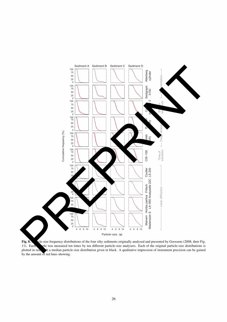
The particle-size distributions analysed by Goossens (2008) are presented in Figure 8. These consist of ten repeat23

measurements of four silty sediment samples A, B, C and D by ten different instruments, giving a total of four hundred24

particle-size distributions. Individual distributions are given in red and the median distribution for each plot is given in25

black. The area of red visible is therefore a qualitative indicator of instrument precision: the more red visible the lower26

the precision.27

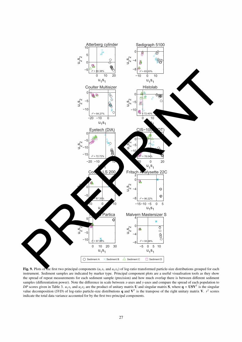
Analytical precision can also be illustrated using principal component analysis (Fig. 9). These plots show the first28

two principal components of each log-ratio particle-size distribution plotted against each other for each technique, which29

account for between 72% and 97% of the population variance. Principal component plots are equivalent to traditional30

mean-sorting plots, but are able to account for the influence of multi-modal distributions on population variability.31

Principal component analysis of particle-size distributions is only feasible in co-ordinate space because the angles between32

particle-size categories are orthogonal. The amount of scatter within each sediment population (Sediments A, B , C or33

11

PREPRINT

D) corresponds inversely to technique precision, noting that the scale of x-axis and y-axis are not equal and that the1

first principal component always describes more variability than the second and so on. For example, the Horiba Partica2

(Horiba Ltd, Kyoto, Japan) and the Fritsch Analysette 22C (Fritsch GmbH, Idar-Oberstein, Germany) both show very low3

total spread for each of the four samples. The principal component scores plot almost on top of each other, so it can be4

said that these techniques have a high precision. In contrast, the spread of principal component scores from the Histolab5

(Microvision Instruments, Evry, France) show that this technique is relatively imprecise.6

The precision of each analytical technique is shown in Table 1, defined as the median ND score between all7

distributions in a population (Eq. 9). The most precise techniques are highlighted in bold for each sediment population.8

Median precision scores for each technique show that there is a marked difference between techniques that use laser9

diffraction (Coulter LS 200 (Beckman Coulter Inc., Fullerton, CA, USA), Fritsch Analysette 22C, Horiba Partica10

LA-950, Malvern Mastersizer S (Malvern Instruments Ltd, Malvern, UK)) and those that rely upon on other physical11

principles. The laser-based techniques all show precision scores lower than 0.029, the Fritsch Analysette 22C achieving12

the best overall score (ND = 0.011). In contrast, the next most precise technique is over an order of magnitude13

less precise. Of the other instruments, settling methods were the next most precise (Atterberg cylinder and Sedigraph14

5100 (Micromeritics Instrument Corporation, Norcross, GA, USA)), followed by electro-resistance (Coulter Multisizer15

3: Beckman Coulter Inc., Fullerton, CA, USA), dynamic image analysis (Eyetech: Ankersmid B.V., Oosterhout, the16

Netherlands), time-of-transition (CIS-100: Galai Production Ltd, now maintained by Ankersmid B.V., Oosterhout, the17

Netherlands) and static image analysis (Histolab).18

Differentiation power19

The difference between sediment samples A, B C and D are quantified as the median ND value between all possible20

combinations of particle-size distributions (Table 2). The results in Table 2 show that the measured difference between21

sediment populations varies with the technique used to analyse particle-size distributions. More importantly, these data22

show that the measured differences between sediments are non-identical. For example, the difference between sediment C23

and D is on average the lowest (ND = 0.11) and the difference between sediment B and C the third lowest (ND = 0.35).24

However, ND scores from the CIS-100 suggest that the difference between sediment B and C is the lowest, and the25

difference between the C and D only the third lowest. Without knowing the precision of the analytical techniques used,26

the meaning and reliability of these scores is unclear.27

To address this problem the measured differences between samples were reanalysed taking into account technique28

precision (Table 1). The resulting Differentiation Power (differentiation power) statistics are presented in Table 3. Values29

highlighted in bold are those that were found to be statistically significant at the 95% confidence level. Scores of one30

indicate that there is no detectable difference between two populations of particle-size distributions (sediment samples)31

when taking into account the precision of the technique with which they were analysed.32

Technique precision and the impact that this has on the potential to differentiate between two sediment samples is33

12

PREPRINT

effectively illustrated by Figure 9. The Histolab has the lowest differentiation power scores on average and is only able1

to differentiate between samples A and C and samples A and D at a 95% confidence level. Figure 9 illustrates that this2

is caused by the high amount of spread and overlap between the principal component scores of the different sediment3

populations. The ND scores between samples given in Table 2 for the Histolab are therefore only valid for comparisons4

between those two pairs of samples. In contrast the Fritsch Analysette 22C showed the highest median DP scores, and5

was able to distinguish between all sediment sediment samples at a 95% confidence level. Figure 9 shows that principal6

component scores for the Fritsch Analysette are very tightly clustered together, with the exception of sediment A. With7

this technique it is therefore possible to differentiate between sediment samples that are very similar at a high confidence8

level.9

Based on average differentiation power scores for all the sample pairs (Table 3) the Fritsch Analysette 22C is the10

technique recommended for analysing samples of slightly clayey silt. differentiation power scores further indicate that of11

the instruments used, those based on laser diffraction-refraction are best at distinguishing between silty sediment samples.12

In addition, whine some instruments are able to differentiate between specific types of sediment to a very high degree,13

they may not necessarily be able to differentiate between other sediment types. For example, the Malvern Mastersizer S,14

while it has a good overall DP score, cannot reliably differentiate between samples A and B.15

Fundamental differences between instruments in terms of how particle-size is measured have been the source of much16

discussion within the research community. Several authors have suggested that sedimentation methods are the most17

appropriate analogies for deposition in marine environments (McCave et al., 2006; McIntyre and Howe, 2009; Bianchi18

et al., 1999). The principal reasons behind this argument have been: (i) particles in the 63 – 10 µm size range preserve the19

most information about sedimentation; and (ii) that laser diffraction instruments tend to underestimate silt to clay-sized20

platy particles relative to sedimentation techniques. It is clear from DP statistics (Table 3) that neither Horiba nor Fritsch21

instruments based on laser diffraction have any difficulty in distinguishing between sediment samples, due to their high22

precision. However, operators preferring to use sedimentation techniques are recommended to use the Atterberg cylinder23

over the Sedigraph 5100. Extension of the present work to encompass a wider range of sedimentary environments would24

provide a much better understanding of the overall capabilities and limitations of these instruments. Such a study would25

require a large inter-laboratory collaboration, as many laboratories analyse only a limited range of sediments.26

Any recommendations made about the appropriateness of a specific analytical technique for sedimentary analysis27

should be based on empirical evidence for a specific range of samples. Averaged values of analytical precision, while28

important, do not fully convey the ability of a technique to distinguish between specific sediments. Indeed, the results29

presented in Table 3 indicate that differentiation power scores should be considered for a range of confidence levels, so30

that the operator is fully aware of the significance of the results produced.31

13

PREPRINT

CONCLUSIONS1

This study presents a methodological framework for the inter-comparison of different particle-size analysers. The2

framework consists of: (i) quantifying differences between complete particle-size distributions; (ii) adjusting for3

differences observed between particle-size distributions measured by different analytical techniques; (iii) quantifying the4

precision of a range of particle-size analysers; and (iv) identifying the most appropriate instrument for analysing a given5

set of samples.6

The main conclusions from this study are presented below.7

1. Then normalized distance statistic provides a means of quantifying differences between particle-size distributions,8

predictive model performance and instrument precision.9

2. Interactive quadratic regression models provide the best means of homogenising data sets of particle-size10

distributions measured by different instruments. Quadratic interaction models allow adjacent particle size-classes11

to be used implicitly to predict logratio transformed percentage values. Quadratic models require a large number of12

training samples (n > 80) compared to linear or polynomial models (n = 50) to achieve optimum results. The ideal13

model therefore depends on the number of samples analysed. The results of cross-validation demonstrated that the14

performance of any regression model is ultimately limited by the precision of the instrument used.15

3. Data presented by Goossens (2008) were used to define the analytical precision of ten different instruments. Those16

instruments based on laser diffraction (Fritsch Analysette 22C, Horiba Partica LA-950, Coulter LS and Malvern17

Mastersizer S) scored markedly higher (two to five times) than settling-based instruments (Atterberg cylinder and18

Sedigraph 5100). The Coulter Multisizer was the next most precise instrument, followed by the CIS-100, the Eyetech,19

with the Histolab instrument scoring the lowest precision value.20

4. The differentiation potential statistic is introduced to assess the significance of differences measured between21

populations of particle-size distributions. Laser diffraction based instruments were best able to distinguish between22

different populations of particle-size distributions at a 95% confidence level. Sedimentation, electro-resistance and23

dynamic image analysis based instruments were also able to differentiate between the majority of silty sediment24

samples, but at a lower degree of precision. In contrast, the Histolab, based on static image analysis performed25

poorly and was only able to differentiate between two populations of sediment samples. The results of this study26

indicate that this instrument is not suitable for the analysis of silty sediments.27

Acknowledgements28

The authors would like to thank the Geological Survey of the Netherlands for database access, Ronald Harting for29

co-ordinating sample logistics and Martin Konert at the Vrije Universiteit Amsterdam for sieve and pipette analysis of30

samples. Simon Blott, Stephen Rice and three anonymous reviewers are thanked for their thorough and thought provoking31

14

PREPRINT

comments on previous versions of this manuscript which have helped to markedly improve it. This work was completed1

when SR was in receipt of a postdoctoral research fellowship at Delft University of Technology, The Netherlands.2

Appendices3

A. Pretreatment of samples for analysis with laser particle sizer4

Measurement of particle-size was performed using a Fritsch A22 XL laser particle sizer. The pretreatment of samples5

and analysis was performed by the following steps.6

1. Gravel content was removed from samples using a 2 mm sieve. Sieved content finer than 2 mm was placed in a in a7

pre-weighed dish and dried in an oven at 70◦C for 48 hours and then weighed.8

2. Subsamples of the dried sediment were added to an 800 mL beaker of distilled water. The amount of sample added9

was dependant on the texture and size range, ∼0.5 g for clays and between 10 and 20 g for sands. The ultimate aim10

was to produce a beam obscuration of 20-25%.11

3. Organic content was removed from the samples by oxidation with H2O2. 5 mL increments of H2O2 were added until12

no further reaction was observed. The excess H2O2 was reduced to a volume of 50-100 mL by boiling.13

4. After cooling, the walls of the beakers were cleaned, to determine the volume of material in suspension.14

5. HCl was added in 5 mL increments until all CaCO in the samples was dissolved. Samples were heated to boiling15

point and topped up with distilled water.16

6. After cooling, samples were measured on a Fritsch A22 XL laser particle sizer, using a KR Helos Quixel dispersion17

unit with a 2 mm cell. Three lenses for three overlapping grain sizes were used with a total of 93 sensor elements,18

of which 59 points were used to calculate particle size. The three ranges were R1 (0.1-35 µm), R4 (1.8-350 µm) and19

R7 (18-3500 µm).20

7. The measurement times were as follows:21

• For the blank or ’background’ measurements were measured in each lens for 10 seconds.22

• The suspension was measured with R1 and R4 for 15 seconds.23

• The suspension was measured with R7 for 45 seconds.24

B. Determination of particle-size distribution by sieve and pipette method25

Samples were prepared for analysis by the following treatment:26

1. Samples were dried at 70◦C for 72 hours.27

2. Samples were then air dried for a further 72 hours in an equilibrium humidity environment.28

15

PREPRINT

3. The moisture content was determined at 50 to 55◦C using a thermogravimetric analyser (LECO TGA 601).1

4. Carbonate content (CaCO3) was calculated as the amount of HCl needed to dissolve the carbonates.2

Measurement of particle-size using the pipette and sieve fractions was performed following the guidelines set out in3

NEN5753. A brief description of this procedure is given below:4

1. Samples were placed in an graded cylinder of distilled water and stirred intensively.5

2. Settling times were calculated at a depth of 20.8 cm using Stoke’s law. Settling velocity v and time for particles to6

reach the calculated depth, were given here as:7

v =

(2(ρs − ρl)gr2

9η

)(12)

where ρs is particle density, ρl is the density of the settling fluid, g is gravitational acceleration, r is particle size and8

η is the viscosity of the settling fluid.9

3. Following this a sample of 20 mL from the calculation depth was taken with a clay-pipette designed following Kohn10

(1928). Each fraction was dried at 40◦C and weighed. The measured weight was corrected for the Na4P2O7 · 10H2O11

addition and percentages.12

4. After the pipette fractions (<2, < 8, <16, <22 and <32 µm) were analysed the remaining sediment was dry sieved13

using a sieve stack ranging from -1 to 4 φ at 0.5 φ intervals.14

C. Data sets15

The data sets analysed in this study can be accessed on-line for download. These are available in CSV formatted files via16

the following links.17

• The simulated data set used in the introduction containing one hundred particle-size distributions :18

http://alturl.com/smrjo19

• Calibration data set containing laser analysis and sieve-pipette analysis measurements :20

http://alturl.com/vmvdo21

• Particle-size distributions from (Goossens, 2008, their Fig. 11) :22

http://alturl.com/2jdiv23

A Matlab function for the automated calculation of ND and DP statistics can be downloaded from the Mathworks file24

exchange (http://www.mathworks.com/matlabcentral/fileexchange/39220). The code is open-source and may25

be modified to run in any equivalent scientific software.26

16

PREPRINT

References

Aitchison, J. (1982). The statistical analysis of compositional data. Journal of the Royal Statistical Society. Series B (Methodological), 44(2), 139–177.Aitchison, J. (1986). The statistical analysis of compositional data: Monographs on statistics and applied probability. Chapman & Hall Ltd., London.Aitchison, J. (1999). Logratios and natural laws in compositional data analysis. Mathematical Geology, 31(5), 563–580.Aitchison, J. (2003). A concise guide to compositional data analysis. In CODAWORK’03. Universitat de Girona. Departament d’Informatica i

Matematica Aplicada, p. 134.Bagnold, R. and Barndorff-Nielsen, O. (1980). The pattern of natural size distributions. Sedimentology, 27, 199–207.Beierle, B. D., Lamoureux, S. F., Cockburn, J. M. and Spooner, I. (2002). A new method for visualizing sediment particle size distributions. Journal

of Paleolimnology, 27(2), 279–283.Beuselinck, L., Govers, G., Poesen, J., Degraer, G. and Froyen, L. (1998). Grain-size analysis by laser diffractometry: comparison with the

sieve-pipette method. Catena, 32(3-4), 193–208.Bianchi, G., Hall, I., McCave, I. and Joseph, L. (1999). Measurement of the sortable silt current speed proxy using the Sedigraph 5100 and Coulter

Multisizer IIe: precision and accuracy. Sedimentology, 46(6), 1001–1014.van den Boogaart, K. G. and Tolosana-Delgado, R. (2008). compositions: A unified R package to analyze compositional data. Computers &

Geosciences, 34(4), 320–338.Buurman, P., Pape, T., Reijneveld, J., De Jong, F. and Van Gelder, E. (2001). Laser-diffraction and pipette-method grain sizing of Dutch sediments:

correlations for fine fractions of marine, fluvial, and loess samples. Geologie en Mijnbouw, 80(2), 49–58.Davis, J. (2002). Statistics and Data Analysis in Geology. 638 pp., Wiley and Sons, New York, third edition.Devore, J. (2011). Probability and Statistics for Engineering and the Sciences. Duxbury Press.Eshel, G., Levy, G., Mingelgrin, U. and Singer, M. (2004). Critical evaluation of the use of laser diffraction for particle-size distribution analysis.

Distribution, 68(3), 736–743.Evans, D. J. and Benn, D. I. (2004). A practical guide to the study of glacial sediments. Arnold London.von Eynatten, H. (2004). Statistical modelling of compositional trends in sediments. Sedimentary Geology, 171(1), 79–89.von Eynatten, H., Barcelo-Vidal, C. and Pawlowsky-Glahn, V. (2003). Composition and discrimination of sandstones: a statistical evaluation of

different analytical methods. Journal of Sedimentary Research, 73(1), 47–57.Falco, G. D., Molinaroli, E., Baroli, M. and Bellaciccob, S. (2003). Grain size and compositional trends of sediments from Posidonia oceanica

meadows to beach shore, Sardinia, western Mediterranean. Estuarine, Coastal and Shelf Science, 58(2), 299 – 309.URL: http://www.sciencedirect.com/science/article/pii/S0272771403000829

Fieller, N., Flenley, E. and Olbricht, W. (1992). Statistics of particle size data. Journal of the Royal Statistical Society. Series C (Applied Statistics),41(1), 127–146.

Folk, R. and Ward, W. (1957). Brazos River bar [Texas]; a study in the significance of grain size parameters. Journal of Sedimentary Research, 27(1),3.

Fredlund, M., Fredlund, D. and Wilson, G. (2000). An equation to represent grain-size distribution. Canadian Geotechnical Journal, 37(4), 817–827.Friedman, G. M. (1962). On sorting, sorting coefficients, and the lognormality of the grain-size distribution of sandstones. The Journal of Geology,

pp. 737–753.Goossens, D. (2008). Techniques to measure grain-size distributions of loamy sediments: a comparative study of ten instruments for wet analysis.

Sedimentology, 55(1), 65–96.Howel, D. (2007). Multivariate data analysis of pollutant profiles: PCB levels across Europe. Chemosphere, 67(7), 1300–1307.Inman, D. (1952). Measures for describing the size distribution of sediments. Journal of Sedimentary Research, 22(3), 125.Jackson, D. (1997). Compositional data in community ecology: The paradigm or peril of proportions? Ecology, 78(3), 929–940.Jonkers, L., Prins, M., Brummer, G., Konert, M. and Lougheed, B. (2009). Experimental insights into laser diffraction particle sizing of fine-grained

sediments for use in palaeoceanography. Sedimentology, 56(7), 2192–2206.Kohn, M. (1928). Beitrage zur Theorie und Praxis der mechanischen Bodenanalyse. Ph.D. thesis, Eberswalde (Forstliche Hochschule).Konert, M. and Vandenberghe, J. (1997). Comparison of laser grain size analysis with pipette and sieve analysis: a solution for the underestimation

of the clay fraction. Sedimentology, 44(3), 523–535.Martın-Fernandez, J., Barcelo-Vidal, C. and Pawlowsky-Glahn, V. (2003). Dealing with zeros and missing values in compositional data sets using

nonparametric imputation. Mathematical Geology, 35(3), 253–278.McCave, I., Hall, I. and Bianchi, G. (2006). Laser vs. settling velocity differences in silt grainsize measurements: estimation of palaeocurrent vigour.

Sedimentology, 53(4), 919–928.McIntyre, K. and Howe, J. (2009). Bottom-current variability during the last glacial-deglacial transition, Northern Rockall Trough and Faroe Bank

Channel, NE Atlantic. Scottish Journal of Geology, 45(1), 43–57.Stauble, D. K. and Cialone, M. A. (1996). Sediment dynamics and profile interactions: Duck94. Coastal Engineering Proceedings, 1(25).Stevens, N. P., Bray, E. E. and Evans, E. D. (1956). Hydrocarbons in sediments of Gulf of Mexico. AAPG Bulletin, 40(5), 975–983.Syvitski, J. (1991). Principles, methods and application of particle size analysis, Cambridge Univ Press, chapter Factor analysis of size frequency

distributions: Significance of factor solutions based on simulation experiments, pp. 249 – 263.Thomas, C. and Aitchison, J. (2006). Log-ratios and geochemical discrimination of Scottish Dalradian limestones: a case study. Geological Society,

London, Special Publications, 264(1), 25–41.Tolosana-Delgado, R. and von Eynatten, H. (2009). Grain-size control on petrographic composition of sediments: compositional regression and

rounded zeros. Mathematical Geosciences, 41(8), 869–886.Tolosana-Delgado, R. and von Eynatten, H. (2010). Simplifying compositional multiple regression: Application to grain size controls on sediment

geochemistry. Computers & Geosciences, 36(5), 577–589.Weltje, G. J. (2002). Quantitative analysis of detrital modes: statistically rigorous confidence regions in ternary diagrams and their use in sedimentary

petrology. Earth-Science Reviews, 57(3), 211–253.Weltje, G. J. (2006). Ternary sandstone composition and provenance: an evaluation of the Dickinson model. Geological Society, London, Special

Publications, 264(1), 79–99.Weltje, G. J. and Prins, M. A. (2003). Muddled or mixed? Inferring palaeoclimate from size distributions of deep-sea clastics. Sedimentary Geology,

162(1-2), 39–62.Weltje, G. J. and Roberson, S. (2012). Numerical methods for integrating particle-size frequency distributions. Computers & Geosciences, 44,

156–167.

17

PREPRINT

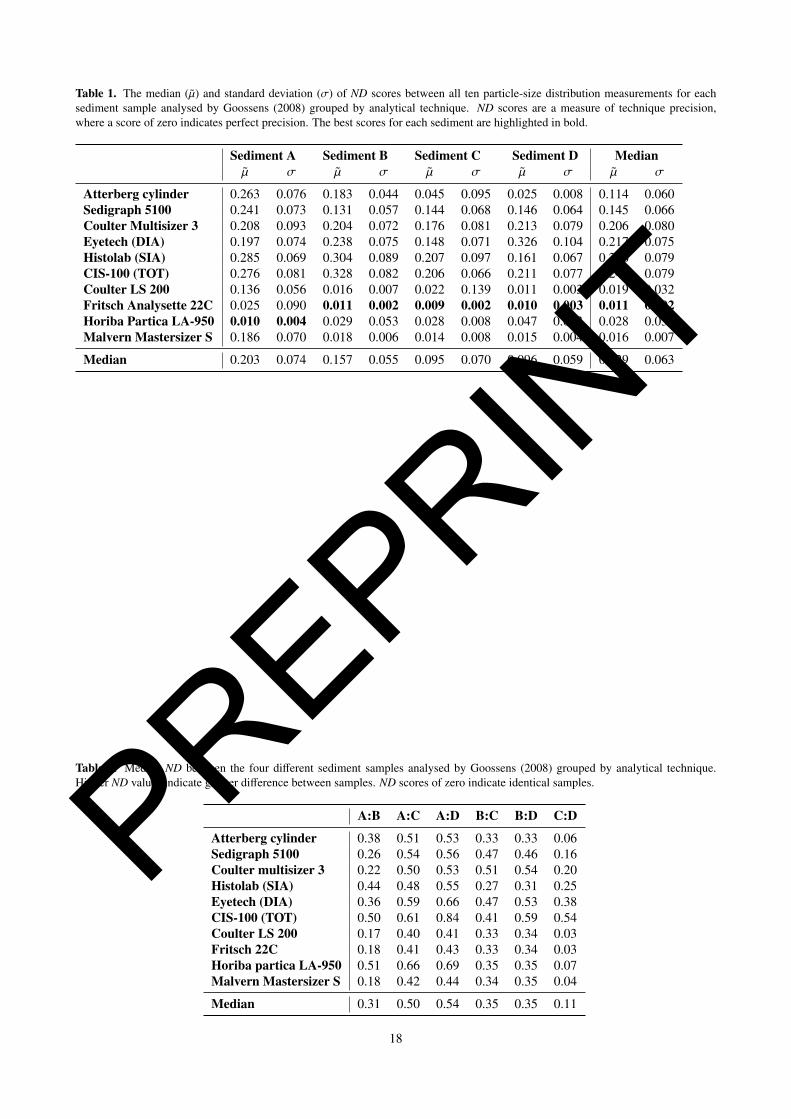
Table 1. The median (µ) and standard deviation (σ) of ND scores between all ten particle-size distribution measurements for eachsediment sample analysed by Goossens (2008) grouped by analytical technique. ND scores are a measure of technique precision,where a score of zero indicates perfect precision. The best scores for each sediment are highlighted in bold.

Sediment A Sediment B Sediment C Sediment D Medianµ σ µ σ µ σ µ σ µ σ

Atterberg cylinder 0.263 0.076 0.183 0.044 0.045 0.095 0.025 0.008 0.114 0.060Sedigraph 5100 0.241 0.073 0.131 0.057 0.144 0.068 0.146 0.064 0.145 0.066Coulter Multisizer 3 0.208 0.093 0.204 0.072 0.176 0.081 0.213 0.079 0.206 0.080Eyetech (DIA) 0.197 0.074 0.238 0.075 0.148 0.071 0.326 0.104 0.217 0.075Histolab (SIA) 0.285 0.069 0.304 0.089 0.207 0.097 0.161 0.067 0.246 0.079CIS-100 (TOT) 0.276 0.081 0.328 0.082 0.206 0.066 0.211 0.077 0.244 0.079Coulter LS 200 0.136 0.056 0.016 0.007 0.022 0.139 0.011 0.003 0.019 0.032Fritsch Analysette 22C 0.025 0.090 0.011 0.002 0.009 0.002 0.010 0.003 0.011 0.002Horiba Partica LA-950 0.010 0.004 0.029 0.053 0.028 0.008 0.047 0.053 0.028 0.030Malvern Mastersizer S 0.186 0.070 0.018 0.006 0.014 0.008 0.015 0.004 0.016 0.007

Median 0.203 0.074 0.157 0.055 0.095 0.070 0.096 0.059 0.129 0.063

Table 2. Median ND between the four different sediment samples analysed by Goossens (2008) grouped by analytical technique.Higher ND values indicate greater difference between samples. ND scores of zero indicate identical samples.

A:B A:C A:D B:C B:D C:D

Atterberg cylinder 0.38 0.51 0.53 0.33 0.33 0.06Sedigraph 5100 0.26 0.54 0.56 0.47 0.46 0.16Coulter multisizer 3 0.22 0.50 0.53 0.51 0.54 0.20Histolab (SIA) 0.44 0.48 0.55 0.27 0.31 0.25Eyetech (DIA) 0.36 0.59 0.66 0.47 0.53 0.38CIS-100 (TOT) 0.50 0.61 0.84 0.41 0.59 0.54Coulter LS 200 0.17 0.40 0.41 0.33 0.34 0.03Fritsch 22C 0.18 0.41 0.43 0.33 0.34 0.03Horiba partica LA-950 0.51 0.66 0.69 0.35 0.35 0.07Malvern Mastersizer S 0.18 0.42 0.44 0.34 0.35 0.04

Median 0.31 0.50 0.54 0.35 0.35 0.11

18

PREPRINT

0 2 4 6 8 10 12−4

−2

0

2

4

6

8

10

Particle−size (φ)

Freq

uenc

y (%

)

Fig. 1. A size-frequency biplot of one hundred simulated particle-size distributionS (grey). The mean and upper and lower 95%confidence levels are plotted respectively as solid, dot-dashed and dashed lines. These have been calculated using percentage-frequencydata (red) and logratio data (black). The upper and lower 95% confidence levels calculated from percentage data violate theconstant-sum constraint, summing respectively to 197.5% and 2.5%. The lower confidence interval calculated from percentage dataare negative, falling outside the parameter space. Confidence intervals calculated from log-ratio values obey both constant-sum andparameter space constraints. Both confidence intervals are predictions of feasible particle-size distributions.

Table 3. Differentiation Power (DP) scores quantify the power of an analytical technique to differentiate between populations ofparticle-size distributions. The DP statistic is the logratio of the median normalised compositional distance between two samplepopulations and the average precision of the technique used for those samples, effectively a signal-to-noise ratio statistic. Thescores here show the ability of each of the ten analytical techniques used by Goossens (2008) to differentiate between populationsof the four silty sediment samples analysed. Scores of one indicate no detectable difference between populations of particle-sizedistributions. Larger scores indicate greater differentiation power. Scores in bold indicate significant different between populations at a95% confidence level.

A:B A:C A:D B:C B:D C:D Median

Atterberg cylinder 1.64 2.57 2.70 2.65 2.73 1.74 2.61Sedigraph 5100 1.35 2.75 2.80 3.39 3.35 1.13 2.77Coulter Multisizer 3 1.07 2.57 2.52 2.66 2.59 1.02 2.54Eyetech (DIA) 1.65 3.33 2.52 2.40 1.88 1.50 2.14Histolab (SIA) 1.51 1.93 2.40 1.06 1.29 1.35 1.43CIS-100 (TOT) 1.65 2.53 3.43 1.51 2.13 2.62 2.33Coulter LS 200 1.75 4.16 4.29 17.16 25.02 1.52 4.23Fritsch Analysette 22C 9.28 21.61 21.27 31.98 31.70 3.03 21.44Horiba Partica LA-950 22.20 30.50 19.46 12.35 9.10 1.70 15.91Malvern Mastersizer S 1.39 3.22 3.31 21.52 21.43 2.93 3.27

Median 1.64 2.98 3.06 3.02 3.04 1.61 2.69

19

PREPRINT

Sand

B

Clay

Silt

00

0

clr(sand)clr(silt)

clr(

clay

)

C

A

Sand

Clay

Silt

Fig. 2. Simulated particle-size distributions (n = 100) summarised by their relative proportions of sand silt and clay, plotted as: (A)A ternary diagram with hexagons of variation delineating confidence regions of the population at 90%, 95% and 99% confidencelevels. Red cross indicates the population mean. (B) A three dimensional scatterplot of centrered log-ratio transformed valuesshowing confidence regions of the population at 90%, 95% and 99% confidence levels. Confidence regions for three orthogonalaxes are calculated as a volume, but are shown here as two dimensional areas for graphic simplicity. (C) A ternary diagram withlogratio confidence regions of the population at 90%, 95% and 99% confidence levels (plotted in (B)) transformed back into percentagefrequency values. Red cross indicates the population mean. In contrast to (A) all areas of the confidence region fall with the parameterspace (0 <= x <= 100).

20

PREPRINT

A B

C D

Unimodal BimodalTrimodal Quadramodal

Fig. 3. Semi-log plots of randomly simulated size-frequency data. Each subplot contains a unimodal, bimodal, trimodal andquadramodal frequency distribution with identical log-normal mean and standard deviation values. These plots illustrate one of thepotential problems involved with using log-normal distribution coefficients to describe complex multimodal particle-size distributions.

21

PREPRINT

0 20 40 60 80 1000

20

40

60

80

100Sand

Data A (% frequency)

Dat

a B

(%−f

requ

ency

) R2 = 0.992β0 = 0.873β1 = 5.939

0 20 40 60 80 1000

20

40

60

80

100Silt

Data A (% frequency)

Dat

a B

(%−f

requ

ency

) R2 = 0.956β0 = 1.047β1 = 2.098

0 20 40 60 80 1000

20

40

60

80

100Clay

Data A (% frequency)

Dat

a B

(%−f

requ

ency

) R2 = 0.446β0 = 0.295β1 = 3.624

−5 0 5−3

−2

−1

0

1

2

3

Sand

Data A (logratio)

Dat

a B

(logr

atio

) R2 = 0.932β0 = 0.696β1 = 0.276

−2 0 2−2

−1

0

1

2Silt

Data A (logratio)

Dat

a B

(logr

atio

) R2 = 0.852β0 = 0.978β1 = 0.100

−2 0 2−3

−2

−1

0

1Clay

Data A (logratio)

Dat

a B

(logr

atio

) R2 = 0.285β0 = 1.200β1 = 0.100

A D

B E

C F

-10

Fig. 4. Biplots of the simulated data set (n = 100) summarised as the relative proportions of sand, silt and clay plotted against anothersimulated data set, replicating the underestimation of clay particles by a laser diffraction based instruments. (A, B, C) Percentage datawith ordinary least-squares linear regression model (red line), model coefficients (β0, β1) and root mean squared error (R). Regressionmodels constructed using percentage data are capable of predicting values outside the mathematical parameter space. These predictions,if corrected post hoc, have implications for the constant-sum constraint. (D, E, F) Log-ratio data with ordinary least-squares linearregression model (red line), model coefficients (β0, β1) and root mean squared error (R). Log-ratio data are free to range between −∞and∞, avoiding the prediction of invalid values. The constant sum constraint is ensured by the back transformation of predicted values(Eq. 3). Note the bias inherent in calculating correlation coefficients (R) of percentage frequency data, which are consistently higherthat for log-ratio data because all the data are positive.

22

PREPRINT

−8 −4 0−8

−4

0

−1.0 φR2 = 0.20

Siev

e−pi

pette

−5 0 5−8

−4

0

−0.5 φR2 = 0.56

−5 0 5

−5

0

50.0 φ

R2 = 0.47

−5 0 5 10

−10−5

05

0.5 φR2 = 0.36

Siev

e−pi

pette

−5 0 5 10−5

0

5

1.0 φR2 = 0.52

−5 0 5−5

0

5

1.5 φR2 = 0.55

−5 0 5−5

0

5

2.0 φR2 = 0.61

Siev

e−pi

pette

−5 0 5−4

0

4

82.5 φ

R2 = 0.52

−5 0 5−2

2

83.0 φ

R2 = 0.47

−5 0 5−2

0246

3.5 φR2 = 0.56

Siev

e−pi

pette

−5 0 5−4

0

64.0 φ

R2 = 0.71

−5 0 5−5

0

5

5.0 φR2 = 0.73

−5 0 5−5

0

5

6.0 φR2 = 0.72

Laser

Siev

e−pi

pette

−5 0 5−5

0

5

7.0 φR2 = 0.66

−5 0 5−5

0

5

8.0 φR2 = 0.63

Laser

−5 0 5−5

0

5

9.0 φR2 = 0.65

Laser

Siev

e−pi

pette

Fig. 5. Plots of log-ratio transformed percentage frequency data comparing laser granulometry data and sieve-pipette data in co-ordinatespace for each of the sixteen particle-size distributions used. Distributions measured by laser analysis have been down-sampled to thesame format as the sieve-pipette data using a log-ratio interpolation algorithm (Weltje and Roberson, 2012). R2 correlation coefficientsshow that there is poor to moderate correlation between the two data sets, with the closest correspondence in the silt to clay sizefractions. In contrast there is relatively poor agreement between the data sets across the sand fraction, caused in this case by zero valuesbeing detected by one instrument and non-zero values being detected by the other.

23

PREPRINT

0

25

50

75

100

ND = 0.533

Sample: 107

0

25

50

75

100

ND = 0.414

0

25

50

75

100

ND = 0.387

0

25

50

75

100

ND = 0.348

Cum

ulat

ive

frequ

ency

(%)

0

25

50

75

100

ND = 0.296

0

25

50

75

100

ND = 0.151

0 2 4 6 80

25

50

75

100

ND = 0.165

ND = 0.248

Sample: 45

ND = 0.225

ND = 0.224

ND = 0.137

ND = 0.155

ND = 0.158

0 2 4 6 8

ND = 0.129

ND = 0.282

Sample: 109

ND = 0.314

ND = 0.423

ND = 0.348

ND = 0.351

ND = 0.189

0 2 4 6 8

ND = 0.229

Particle−size (φ)

ND = 0.516

Sample: 66

ND = 0.544

ND = 0.512

ND = 0.358

ND = 0.249

ND = 0.189

0 2 4 6 8

ND = 0.136

ND = 0.683

Sample: 5

Sie

ve−p

ipet

te

ND = 0.704

Line

ar

ND = 0.704 2nd

o

rder

poly

nom

ial

ND = 0.536

3−te

rmqu

adra

ticND = 0.433

5−te

rm q

uadr

atic

with

inte

ract

ion

ND = 0.278

7−te

rm q

uadr

atic

with

inte

ract

ion

0 2 4 6 8

ND = 0.248

9−te

rm q

uadr

atic

with

inte

ract

ion

Fig. 6. Cumulative frequency distribution plots for five randomly selected sediment samples from the Dutch data set showing theresults of six different regression models applied to predict equivalent laser measurements from sieve-pipette data. The first row showmeasured sieve-pipette data (red-dashed line) plotted against laser analysis data (black solid line). Cumulative-frequency plots inrows two to seven compare laser analysis data (solid black line) with the results of a range of regression models: (i) linear, (ii) 2nd

order polynomial, (iii) three-term quadratic, (iv) five-term quadratic with interaction, (v) seven-term quadratic with interaction and (vi)nine-term quadratic with interaction. Model performance is quantified using the ND statistic (Eq. 9). Note that an increase in thenumber of model terms does not automatically guarantee a better prediction, and that not all regression models offer an improvementover the original sieve-pipette measurements.

24

PREPRINT

0 20 40 60 80 100 120 1400

0.1

0.2

0.3

0.4

0.5

0.6

0.7

0.8

0.9

1

Number of training samples

ND

A

20 40 60 80 100 1202

3

4

5

6

7

8

9

10

0.41

B

20 40 60 80 100 1202

3

4

5

6

7

8

9

10

0.41

C

20 40 60 80 100 1202

3

4

5

6

7

8

9

10

0.230.4

1

D

ND0 0.1 0.2 0.3 0.4 0.5 0.6 0.7 0.8 0.9 1

Num

ber o

f mod

el c

oeffi

cien

ts

140

140140

Num

ber o

f mod

el c

oeffi

cien

tsN

umbe

r of m

odel

coe

ffici

ents

Number of training samples

Number of training samplesNumber of training samples

Fig. 7. The results of cross-validation showing the performance of regression models as a function of the number of samples used toconstruct regression models (A to D) and the number of model coefficients used (B to D). (A) Performance of linear regression modelin co-ordinate space shows that the best model performance is achieved with 118 samples (ND = 0.35), although model performancewith only 38 training samples is almost as good (ND = 0.35). Dot-dashed line in (A) indicates goodness-of-fit between laser data andsieve-pipette data. Precision of sieve-pipette analysis is shown by a dotted line and the precision of laser analysis by a dashed line.(B) Performance of polynomial regression model in co-ordinate space show that low performance gains are to be had by increasing thenumber of training samples or model coefficients. White contour lines at 0.41 in plots (B) to (D) indicate the goodness-of-fit betweenlaser data and sieve-pipette data. Models with scores lower than 0.41 should not be used. (C) Results of quadratic regression modelshows that discernible improvements in model performance can be made by using both more training samples and model coefficients.(D) Quadratic interaction regression models provide the best method of homogenising sieve-pipette and laser particle-size distributions.Contour line at 0.23 corresponds with the precision of sieve-pipette analysis and hence the limit of the models’ predictive performance.Performance scores higher than this are the result of modelling noise in the data. The best model to use ultimately depends on theavailable number of samples, although the use of fewer coefficients will limit computational overhead.

25

PREPRINT

0255075

100Sediment A

0255075

100

0255075

100

0255075

100

0255075

100

Cum

ulat

ive

frequ

ency

(%)

0255075

100

0255075

100

0255075

100

0255075

100

4 6 8 100

255075

100

Sediment B

4 6 8 10

Particle−size (φ)

Sediment C

4 6 8 10

Sediment D

Atte

rber

gcy

linde

rC

IS−1

00C

oulte

rLS

200

Cou

lter

mul

tisiz

er 3

Eye

tech

(DIA

)Fr

itsch

Ana

lyse

tte 2

2CH

isto

lab

(SIA

)H

orib

a pa

rtica

LA−9

50M

alve

rnM

aste

rsiz

er S

4 6 8 10

Sed

igra

ph51

00

Lase

r diff

ract

ion

Sed

imen

tatio

nE

lect

ro-

resi

stan

ceTi

me

of

trans

ition

Imag

e an

alys

is

Fig. 8. Particle-size frequency distributions of the four silty sediments originally analysed and presented by Goossens (2008, their Fig.11). Each sample was measured ten times by ten different particle-size analysers. Each of the original particle-size distributions isplotted in red, with a median particle-size distribution given in black. A qualitative impression of instrument precision can be gainedby the amount of red lines showing.

26

PREPRINT

0 10 20

−5

0

5

10Atterberg cylinder

u1s1u 2s 2

r2 = 80.38%

−20 0 20−15

−10

−5

0

5CIS−100 (TOT)

u1s1

u 2s 2

r2 = 78.04%

−10 0 10

−5

0

5

Coulter LS 200

u1s1

u 2s 2

r2 = 87.35%

−20 −10 0

−10

−5

0Coulter Multisizer

u1s1

u 2s 2

r2 = 84.27%

−20 −10 0 10

−15

−10

−5

0Eyetech (DIA)

u1s1

u 2s 2

r2 = 72.72%

−15−10 −5 0 5

−8

−4

02

Fritsch Analysette 22C

u1s1

u 2s 2

r2 = 96.22%

0 10 20

−10

−5

0

Histolab

u1s1u 2s 2

r2 = 72.40%

0 10 20 30

−10

−5

0

5Horiba Partica

u1s1

u 2s 2

r2 = 97.96%

−5 0 5 10−8

−4

0

4Malvern Mastersizer S

u1s1

u 2s 2

r2 = 93.68%

−10 0 10

−8

−4

0

Sedigraph 5100

u1s1

u 2s 2

r2 = 83.20%

Sediment A Sediment B Sediment C Sediment D

Fig. 9. Plots of the first two principal components (u1 s1 and u2 s2) of log-ratio transformed particle-size distributions grouped for eachinstrument. Sediment samples are indicated by marker type. Principal component plots are a useful visualisation tools as they showthe spread of repeat measurements for each sediment sample (precision) and how much overlap there is between different sedimentsamples (differentiation power). Note the difference in scale between x-axes and y-axes and compare the spread of each population toDP scores given in Table 3. u1 s1 and u2 s2 are the product of unitary matrix U and singular matrix S, where q = USVT is the singularvalue decomposition (SVD) of log-ratio particle-size distributions q and VT is the transpose of the right unitary matrix V. r2 scoresindicate the total data variance accounted for by the first two principal components.

27

PREPRINT