integrating a random utility model for non-timber forest users into a strategic forest planning...

ARTICLE IN PRESS

Journal of Forest Economics 14 (2008) 133–153

1104-6899/$ -

doi:10.1016/j

�CorrespoE-mail ad

1Tel.: +1 7

www.elsevier.de/jfe

Integrating a random utility model for non-timber forest users

into a strategic forest planning model

David M. Nananga,�, Grant K. Hauerb,1

aIndian and Northern Affairs Canada, 10 Wellington Street, Gatineau, Quebec,

Canada K1A 0H4bDepartment of Rural Economy, University of Alberta, Edmonton, Alberta, Canada T6G 2H1

Received 2 February 2006; accepted 16 August 2007

Abstract

In this paper, we developed a mixed-integer non-linear programming model that integrates

access road development and a utility theoretic spatial choice model of hunters into a strategic

forest harvest-scheduling model. The model was applied to an operationally sized Forest

Management Agreement (FMA) area in central Alberta, Canada. The resulting behavioral model

had approximately 2.6 million decision variables and about 96,000 constraints, and was used to

examine the impacts of timber harvesting on hunters’ preference for hunting sites. We also

evaluated the impacts of various levels of hunter welfare on: (i) the degree of tradeoff between

timber and hunting benefits, (ii) timber harvest schedules, and (iii) the marginal costs of producing

timber products. The results showed significant tradeoffs between timber and hunting benefits and

a clear link between landscape characteristics and changes and behavioral responses by hunters.

r 2007 Elsevier GmbH. All rights reserved.

JEL classification: Q230

Keywords: Decomposition techniques; Harvest-scheduling; Random utility model; Landscape;

Recreational hunting

see front matter r 2007 Elsevier GmbH. All rights reserved.

.jfe.2007.08.001

nding author. Tel.: +1819 953 9706; fax: +1 819 953 2454.

dresses: [email protected] (D.M. Nanang), [email protected] (G.K. Hauer).

80 492 0820; fax: +1 780 492 0268.

www.elsevier.de/jfe

dx.doi.org/10.1016/j.jfe.2007.08.001

mailto:[email protected]

mailto:[email protected]

ARTICLE IN PRESS

D.M. Nanang, G.K. Hauer / Journal of Forest Economics 14 (2008) 133–153134

Introduction

Increasing public demand for non-timber goods and services from forests hasprovided the motivation for forest managers to incorporate these benefits intostrategic forest management planning. Incorporating non-timber values intotraditional timber supply models has the potential to change optimal rotation agesand consequently affect timber harvest schedules. Furthermore, non-timber valuesaffect the normal issues of choosing stands for harvest to achieve concentration inspace as well as profitability based only on timber values. Concentration is desiredover space because of economies of scale associated with concentrating harvests overthe landscape. Forest operations such as harvesting and road construction also affectwildlife and other non-timber values within the forest. When multiple forest benefitsare considered, forest management activities become interdependent, and any oneactivity ultimately affects other values directly or indirectly.

The challenge for forest managers is not only how to incorporate these multiplevalues into existing forest planning models, but also to understand the nature anddegree of tradeoffs that may be associated with the provision of multiple benefits. Tounderstand these tradeoffs, we need to know the nature of the relationships betweenthe various forest uses. Determining the relationships between the various forest usesis a task of considerable complexity, though these relationships are known to fallinto three main categories: independent, complementary, or competitive (Teeguarden,1982). One way to evaluate these tradeoffs is to integrate timber and non-timbervalues into forest management scheduling models. Whilst timber output levels areoften easy to set, it is usually difficult to determine how much non-timber goods andservices to produce and where, and the effect of timber management activities onnon-timber users of the forests. These and other multiple-use questions arefundamental to long-term planning that ensures the sustainability of forests andallows society to derive maximum benefits from forest resources.

This paper provides an effort to incorporate a specific type of non-timber valueinto a strategic forest management model. We developed a utility theoretic spatialchoice model and applied it to a Forest Management Agreement (FMA) area inAlberta, Canada. We use mixed-integer non-linear programming (MINLP) toincorporate a spatially explicitly utility function for hunter recreation values into aforest level harvest scheduling and access road development model. The resultingbehavioral model was used to examine the impacts of various levels of hunter welfareon: (i) the degree of tradeoff between timber and hunting benefits, (ii) timber harvestschedules, and (iii) the marginal costs of producing timber products. Because of theimportance of hunting to many communities in Alberta, this activity is used as anexample to investigate the above objectives, which we believe are crucial to analysesof tradeoffs arising from conflicts in providing timber and non-timber benefits. Thispaper contributes significantly to our understanding of the link between landscapecharacteristics and changes and behavioral responses by hunters and recreationists.This knowledge is important if the prediction of how hunting patterns will change inresponse to different management scenarios is required. It is important to emphasizethat though our specification of non-timber values is not exhaustive, the methods

ARTICLE IN PRESS

D.M. Nanang, G.K. Hauer / Journal of Forest Economics 14 (2008) 133–153 135

shown here demonstrate how other behavioral models for other forms of hunting,recreation and fishing for example, could be incorporated.

This is not the first attempt to incorporate non-timber values of forests intomathematical programming models. The literature abounds with examples ofdifferent approaches to model multiple objectives of forest management usingmathematical programming. Although these references are not intended to beexhaustive, they clearly show the level of interest by researchers, and the range oftechniques that have been employed, to incorporate non-timber values intomathematical programming timber supply models. The earliest and most widelyused technique is goal programming, which was pioneered by Field (1973).Following the work of Field (1973), many other researchers have applied goalprogramming to different forest management problems, for example Kao andBrodie (1979), Field et al. (1980), and Diaz-Balteiro and Romero (1997). Thoughgoal programming may be adequate for examining tradeoffs in forest managementwith multiple criteria, it suffers from the possibility of dominated solutions, andproblems with goal and utility functions specification (Bouzaher and Mendoza,1987).

Despite the popularity of goal programming, other approaches that addressmultiple objectives of forest management have been applied to forest problems. Onesuch approach is the optimization of timber values with spatial and/or temporal(e.g., green up) constraints to protect non-timber resources such as wildlife, waterquality, aesthetics, and increased recreational opportunities (e.g., Carter et al., 1997;Nelson et al., 1993). A third approach is the use of utility functions to compare theutility from multiple objective functions, which represent the utility obtained fromvarious timber and non-timber forest products. The various objective functions areoptimized using alternative management schedules, and the management schedulethat results in the highest utility is chosen (e.g., Harrison and Rosenthal, 1986;Kilkki et al., 1986; Kangas and Pukkala, 1996).

The next generation of modeling timber and non-timber benefits sought toovercome the limitations of previous models by incorporating spatial and temporaldimensions and using forest landscapes of more realistic sizes (e.g., Montgomery etal., 1999; Lichtenstein and Montgomery, 2003). A key drawback of static and non-spatial models is that they may prescribe management regimes that are infeasible orincorrectly estimate the productive capacity of landscapes (Nalle et al., 2004). Afurther improvement to these static models was the introduction of dynamics intothe modeling approach, such as that of Hof and Raphael (1997). However, most ofthese dynamic models either lacked the complexity or scale of actual forestlandscapes.

This paper extends previous studies in several ways. First, most of the previousapplications reported were small forest problems with limited spatial resolution. Weapplied the modeling technique to an operationally sized FMA in Alberta, which islarge enough to provide meaningful results for policy formulation regardingmultiple-use of forest lands. Given that forest management areas of this size are therule rather than the exception in Canada, developing modeling techniques that solvelarge, spatially and temporally detailed models in relatively short computer time is

ARTICLE IN PRESS


both attractive and necessary. Secondly, we use a site choice model (random utilitymodel), which is widely used in the literature to model consumer choice from amonga discrete set of alternatives such as in recreation demand (Adamowicz et al., 1997).The approach results in a behavioral model, in that as the characteristics of the forestchange, the expected behavior of hunters change and so do the expected benefits.This therefore allows for the possibility of substitution among hunting sites overtime, which is endogenously driven by changes in the characteristics of the forest.Furthermore, our model explicitly considers road access development, which allowsus to examine the long-term impacts of access road development on non-timberbenefits. Although modeling road access complicates the modeling and solution ofthe problem, it is an extremely important factor in determining harvesting andhunter preferences on the landscape.

The next section of this paper gives a detailed description of the MINLPformulation. The results from an empirical application of the model to anoperationally sized forest management problem is then presented, followed by adiscussion of the management applications of the results, and possible extensions ofthe present model. The conclusions from the results are presented in the last section.

Model formulation

To ease comparison of this model with others in the literature, we present theexplicit mathematical formulation for the forest management problem. The model isan extension of the Model II formulation given in Johnson and Scheurman (1977).

First, we define the following sets and variables:Let

J be the set of all supply locations in the forest with j serving as a counter(j ¼ 1,y,J)JP be the set of permanently accessed supply locationsJ1 be the set of all permanently accessed locations that are adjacent to at least onelocation that is not accessedI be the set of all demand locations with i serving as a counter (i ¼ 1,y,I)IjA be the set of all supply locations adjacent to j from which product may be

shipped. This set is empty for all j 2 Jp � J1 (i.e., permanently opened locationsthat are not adjacent to any unaccessed locations)IjB be the set of all supply locations adjacent to j to which product may be shipped

IjC be the set of all demand locations to which product may be shipped from j. This

set is empty for all jeJp. Note that j is only aplicable to permanently accessedlocations.ypjit be the volume shipped from supply location j to demand location i for j 2 Jp.

yAjkt be the volume shipped from supply location j to supply location k for j; keJp

and j 2 J1.ys

jt be the volume supply at location j.

ARTICLE IN PRESS


ydit be the volume demand at demand location i.

zjt be the 0,1 access variable for location j.

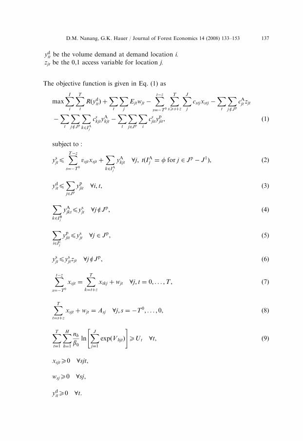
The objective function is given in Eq. (1) as

maxXI

i

XT

t

RðyditÞ þ

Xt

Xj

Ejtwjt �Xt�z

s¼�T0

XT

sXsþz

XJ

j

cstjxstj �X

t

XjeJp

cAjt zjt

�X

t

XjeJp

Xk2IAj

cskjty

Akjt �

Xt

Xj2Jp

Xi

csjity

pjit, ð1Þ

subject to :

ysjtp

XT�z

s¼�T0

vsjtxsjt þXk2IAj

yAkjt 8j; tðIAj ¼ f for j 2 Jp � J1Þ, ð2Þ

yditp

Xj2Jp

ypjit 8i; t, (3)

Xk2IBj

yAjktpys

jt 8jeJp, (4)

Xi2I cj

ypjitpys

jt 8j 2 Jp, (5)

ysjtpys

jtzjt 8jeJp, (6)

Xt�z

s¼�T0

xsjt ¼XT

k¼tþz

xtkj þ wjt 8j; t ¼ 0; . . . ;T , (7)

XT

t¼sþz

xsjt þ wjt ¼ Asj 8j; s ¼ �T0; . . . ; 0, (8)

XT

t¼1

XHh¼1

nh

b0lnXJ

j¼1

expðV hjtÞ

" #XUt 8t, (9)

xsjtX0 8sjt,

wsjX0 8sj,

yditX0 8t.

ARTICLE IN PRESS


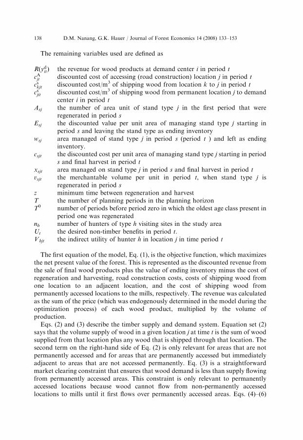
The remaining variables used are defined as

RðyditÞ the revenue for wood products at demand center i in period t

cAjt discounted cost of accessing (road construction) location j in period t

cskjt discounted cost/m3 of shipping wood from location k to j in period t

csjit discounted cost/m3 of shipping wood from permanent location j to demandcenter i in period t

Asj the number of area unit of stand type j in the first period that wereregenerated in period s

Esj the discounted value per unit area of managing stand type j starting inperiod s and leaving the stand type as ending inventory

wsj area managed of stand type j in period s (period t ) and left as endinginventory.

csjt the discounted cost per unit area of managing stand type j starting in periods and final harvest in period t

xsjt area managed on stand type j in period s and final harvest in period t

vsjt the merchantable volume per unit in period t, when stand type j isregenerated in period s

z minimum time between regeneration and harvestT the number of planning periods in the planning horizonT0 number of periods before period zero in which the oldest age class present in

period one was regeneratednh number of hunters of type h visiting sites in the study areaUt the desired non-timber benefits in period t.V hjt the indirect utility of hunter h in location j in time period t

The first equation of the model, Eq. (1), is the objective function, which maximizesthe net present value of the forest. This is represented as the discounted revenue fromthe sale of final wood products plus the value of ending inventory minus the cost ofregeneration and harvesting, road construction costs, costs of shipping wood fromone location to an adjacent location, and the cost of shipping wood frompermanently accessed locations to the mills, respectively. The revenue was calculatedas the sum of the price (which was endogenously determined in the model during theoptimization process) of each wood product, multiplied by the volume ofproduction.

Eqs. (2) and (3) describe the timber supply and demand system. Equation set (2)says that the volume supply of wood in a given location j at time t is the sum of woodsupplied from that location plus any wood that is shipped through that location. Thesecond term on the right-hand side of Eq. (2) is only relevant for areas that are notpermanently accessed and for areas that are permanently accessed but immediatelyadjacent to areas that are not accessed permanently. Eq. (3) is a straightforwardmarket clearing constraint that ensures that wood demand is less than supply flowingfrom permanently accessed areas. This constraint is only relevant to permanentlyaccessed locations because wood cannot flow from non-permanently accessedlocations to mills until it first flows over permanently accessed areas. Eqs. (4)–(6)

ARTICLE IN PRESS


define the access and wood transport from one supply location to another supplylocation and from supply locations to mills. Eq. (4) states that the volume of woodshipped from one location to another location cannot be greater than the volumesupply of wood in the initial location. Eq. (5) implies that the volume of woodshipped from a permanently accessed location to a mill cannot be greater than thevolume supply of wood in the supply location. Eqs. (4) and (5) taken togethersuggest that wood flows from one location to another in the locations that are notpermanently accessed, whilst in permanently accessed locations, wood is shippeddirectly from supply locations to the mills. Eq. (6) constrains the model to ensurethat each location without permanent access is accessible when it is to be harvested.That is, access must first be provided before harvesting can take place. It isimportant to notice that Eq. (6) is quite different from the rest in that it is a non-linear constraint in which the access variable (zjt) is a binary integer variable. Thisequation could also be written as ys

jtpzjtM, where M is a large number. This is thestandard way of writing such a constraint. However, here we use the form in Eq. (6)due to the fact that we applied the dual decomposition approach that uses heuristicsto adjust dual prices on constraints. We find that the constraint as written in Eq. (6)provides a more convenient interpretation of the dual price and heuristics for priceadjustment (see Appendix A).

Eqs. (7) and (8) describe the forestland constraints including the initial age classdistribution and the dynamics of transition from harvest to regenerated stands.These two equations are part of the standard Model II set-up of Johnson andScheurman (1977).

Eq. (9) is the hunter welfare constraint and implies that the non-timber benefitsderived by hunters in the FMA should not be less than a specified value Ut. Thehunter welfare on the left-hand side of Eq. (9) was estimated based on the indirectutility function described in Eq. (10). These benefits are endogenously determined bythe model, such that as the characteristics of the forest change due to harvesting, sodo the benefits.

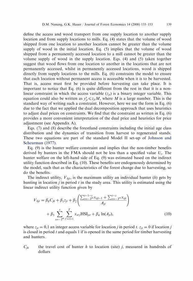
The indirect utility, V hjt, is the maximum utility an individual hunter (h) gets byhunting in location j in period t in the study area. This utility is estimated using thelinear indirect utility function given by

Vhjt ¼ b0Cjh þ b1zjt þ b2

Pt�1�zs¼�T0xsjt�1 þ

Pt�zs¼�T0xsjt

Ajt

!

þ b3Xt

s¼�T0

XT

t0¼tþ1

xst0jHSIjst þ b4 lnðAjtÞ, ð10Þ

where zjt ¼ 0,1 an integer access variable for location j in period t. zjt ¼ 0 if location j

is closed in period t and equals 1 if is opened in the same period for timber harvestingand hunters.

Cjh the travel cost of hunter h to location (site) j, measured in hundreds ofdollars

ARTICLE IN PRESS


Ajt total forested area (in km2) of location (site) j in period tPt�1�zs¼�T0xsjt�1 the total area harvested in location j in the previous period (t�1)Pt�zs¼�T0xsjt the total area harvested in location j in period t

HSIjst the average Habitat Suitability Index (HSI) of location j at time t for stands

born in time s. This HSI comes from the study of Buckmaster et al. (1999).

The HSI is a rating between zero (very poor habitat) and one (very good habitat)of the quality of a site for a particular animal species. HSI models predict thesuitability of a habitat for species based on an assessment of habitat attributes suchas habitat structure, habitat type and spatial arrangements between habitat features(Buckmaster et al., 1999). For forested areas of the FMA, this is calculated asHSIijst ¼ S2S3, where S2 is the HSI associated with percent tree canopy closure, andS3 represents the HSI associated with per cent deciduous tree canopy cover (percentcomposition of deciduous tree species in the tree canopy). From the definition of theHSI for the stands, we can obtain the average HSI (weighted by the area of stands)for location j in period t as

HSIjst ¼1

Ajt

XI

i¼1

Xt

s¼�T0

XT

t0¼tþ1

xist0jHSIijst.

The final measure of a site’s quality, however, is the elk habitat units (EHU),which is obtained by multiplying the HSI of a stand by its corresponding area, whichis used in Eq. (10). Note we are summing up HSIs for stands born before time t butwhich are also harvested after time t in period t0.

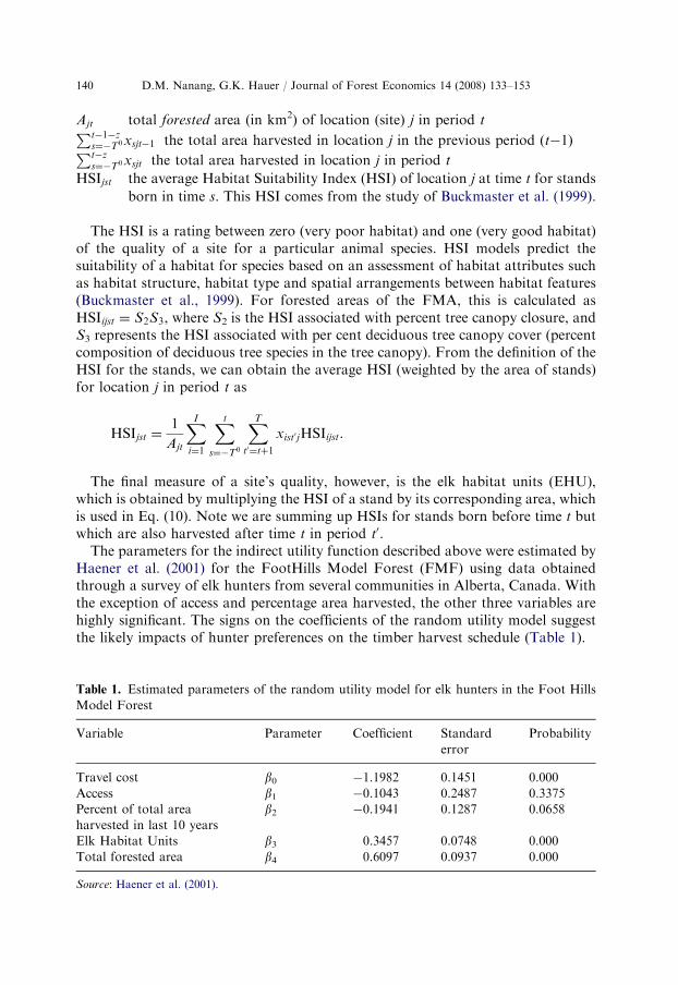
The parameters for the indirect utility function described above were estimated byHaener et al. (2001) for the FootHills Model Forest (FMF) using data obtainedthrough a survey of elk hunters from several communities in Alberta, Canada. Withthe exception of access and percentage area harvested, the other three variables arehighly significant. The signs on the coefficients of the random utility model suggestthe likely impacts of hunter preferences on the timber harvest schedule (Table 1).

Table 1. Estimated parameters of the random utility model for elk hunters in the Foot Hills

Model Forest

Variable Parameter Coefficient Standard

error

Probability

Travel cost b0 �1.1982 0.1451 0.000

Access b1 �0.1043 0.2487 0.3375

Percent of total area

harvested in last 10 years

b2 �0.1941 0.1287 0.0658

Elk Habitat Units b3 0.3457 0.0748 0.000

Total forested area b4 0.6097 0.0937 0.000

Source: Haener et al. (2001).

ARTICLE IN PRESS


Study area and problem definition

The problem being addressed in this study can be described as using optimizationtechniques to formulate and solve a large integrated forest-scheduling model. Usingspatial data from geographic information system (GIS), a FMA area ofapproximately 640,000 ha in central Alberta, Canada was aggregated into 577locations (of about 1100 ha each). The problem therefore, was to maximize thepresent value of wood scheduled on these locations less harvest, transportation,regeneration, and road building costs, subject to several constraints including ahunter benefit constraint. There are two demand centers, labeled A and B. DemandCenter A serves as a demand center for the two wood products, lumber and orientedstrand board (OSB), and also as an entry point for hunters into the FMA. DemandCenter B only serves as an entry point for hunters.

We define the number of decision variables and constraints to the above problemusing a planning horizon of 100 years with 10 planning periods, a minimum rotationof 40 years, three regeneration prescriptions per stand (natural regeneration, basic,and intensive silviculture), a total of 6156 stand types, 18,883 analysis areas, andapproximately six shipping alternatives for each stand. With these assumptions, theresulting model has approximately 2.6 million decision variables and about 96,000constraints.

Incorporating access development and constraints complicates model formulationand solution in several ways. First, access constraints impose both temporal andspatial requirements on the model and hence considerably increase the number ofdecision variables and constraints to be modeled. Secondly, because adequate accessmust be provided before forest management activities can be carried out in forests, itplaces constraints on where timber can be harvested in any given period. Thirdly,simultaneous optimization of forest management activities, access and non-timberbenefits using mixed-integer programming is easy to solve for small models.However, the difficulty of solving such models increases as the number of decisionvariables and constraints increase.

To ease the difficulties introduced by the access integer variables, we definelocations that currently have a major road through them as permanently opened/accessed locations (POLs). These POLs are assumed to be built and maintained ingood condition throughout the planning horizon at some fixed cost. Temporary orintermittent roads are built to each location in each planning period as needed. Toreduce the problem to a reasonable level of complexity, we did not explicitly modeltemporary roads built to access stands within locations. We find the cost-minimizingroad network to connect all locations targeted for harvests to the existing roads.Locations to be harvested are determined based on economic criteria of timber andnon-timber benefits of accessing a location exceeding the costs of doing so.

The number of integer decision variables in this formulation is estimated at 3850,which in a branch and bound algorithm would have 23850 combinations of solutionsalthough the number of combinations that actually need to be explored is somewhatless than this because of the constraints on sequencing. For example, some locationswould have to be accessed through other locations. Even then, it is obvious that the

ARTICLE IN PRESS


enormous number of feasible solutions associated with this problem will make it anextremely difficult problem to solve using the branch and bound technique. Thesolution algorithm we employ breaks down the large MINLP problem into simplestand level economic analysis over the planning horizon, and simple optimal pathnetwork analysis for access planning in each planning period given the value ofcurrent dual prices. Simple intuitive price adjustment procedures are used to changedual prices to move the solution towards feasibility.

The model was solved using a variant of the dual decomposition algorithmproposed by Hoganson and Rose (1984). Only the general outline is discussed here.The detailed algorithm for the solution is given in Appendix A. First, we assumedthat all the POLs are opened in each time period throughout the planning horizon.All other areas are considered closed at the beginning of each model run, and theseclosed areas are sorted according to how far away they are from a POL, startingfrom those locations that are directly adjacent to POLs, those that are one locationaway, etc. There were 192 POLs (zjt ¼ 1), and 385 closed (zjt ¼ 0) locations at thebeginning of each model run. The solution algorithm for this problem describedbelow is based on the first-order conditions of the lagrangian function derived fromEqs. (1)–(9). The algorithm begins by solving each stand level problem using initialguesses at the shadow prices for each forest wide constraint for both POLs andinitially closed locations. These stand level decisions include harvest timing for initialand subsequent harvests, mill destination for each timber type, and regenerationoptions. After all of the stand level problems are solved, the volume flows implied bythe harvest timing and transport options are added up and compared to the demandconstraint levels for timber products. If the flows deviate from the constraint levelsand mill demand levels then the shadow prices are adjusted using simple intuitiveshadow price adjustment procedures described by Hoganson and Rose (1984) andmodified by Hauer (1993).

Model scenarios

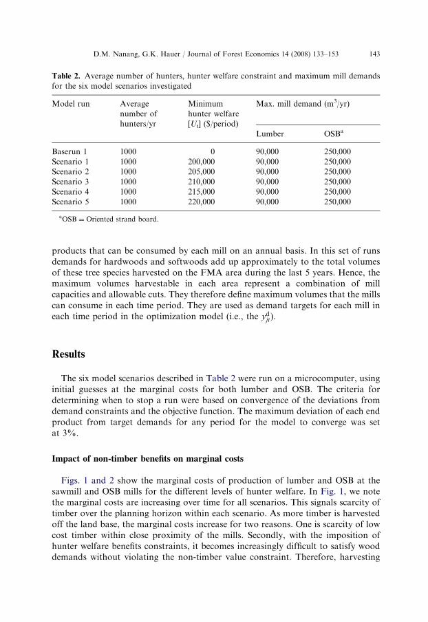
To achieve the objectives of this paper, we examined six different scenarios of themodel specified above. Each model run is comprised of combinations of the samelevels of timber volumes harvested, average number of hunters visiting the studyarea, and different levels of hunter benefits specified in Table 2. The second columnin Table 2 shows the average number of hunters that visit a location in any givenyear. The hunters visit the study area either from Demand Center A or DemandCenter B. The number of hunters was estimated based on the sales of elk huntinglicences for the study area from the Fish and Wildlife Division of AlbertaEnvironment (Alberta Environment, 2001). The third column specifies the maximumnon-timber value (hunter welfare) constraint, in terms of dollars per planning period.The range of values for this constraint was determined by first running the modelwithout a non-timber constraint in order to estimate the range of non-timber benefitsin each planning period. The last two columns give the maximum volume of final

ARTICLE IN PRESS

Table 2. Average number of hunters, hunter welfare constraint and maximum mill demands

for the six model scenarios investigated

Model run Average

number of

hunters/yr

Minimum

hunter welfare

[Ut] ($/period)

Max. mill demand (m3/yr)

Lumber OSBa

Baserun 1 1000 0 90,000 250,000

Scenario 1 1000 200,000 90,000 250,000

Scenario 2 1000 205,000 90,000 250,000

Scenario 3 1000 210,000 90,000 250,000

Scenario 4 1000 215,000 90,000 250,000

Scenario 5 1000 220,000 90,000 250,000

aOSB ¼ Oriented strand board.


products that can be consumed by each mill on an annual basis. In this set of runsdemands for hardwoods and softwoods add up approximately to the total volumesof these tree species harvested on the FMA area during the last 5 years. Hence, themaximum volumes harvestable in each area represent a combination of millcapacities and allowable cuts. They therefore define maximum volumes that the millscan consume in each time period. They are used as demand targets for each mill ineach time period in the optimization model (i.e., the yd

jt).

Results

The six model scenarios described in Table 2 were run on a microcomputer, usinginitial guesses at the marginal costs for both lumber and OSB. The criteria fordetermining when to stop a run were based on convergence of the deviations fromdemand constraints and the objective function. The maximum deviation of each endproduct from target demands for any period for the model to converge was setat 3%.

Impact of non-timber benefits on marginal costs

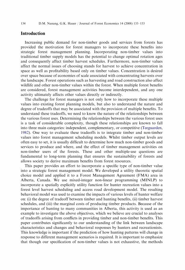
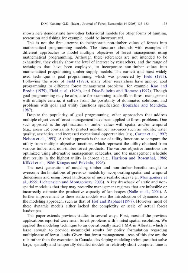
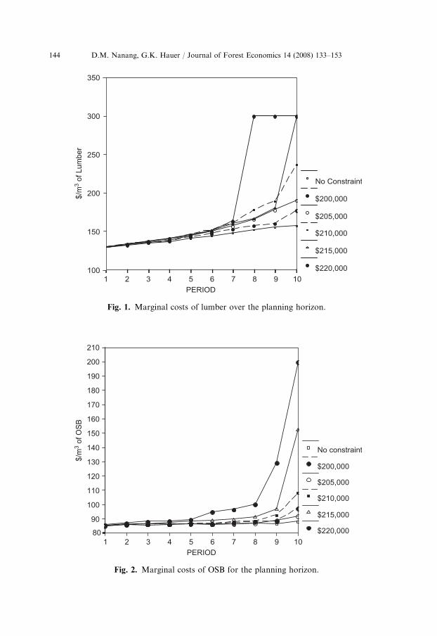
Figs. 1 and 2 show the marginal costs of production of lumber and OSB at thesawmill and OSB mills for the different levels of hunter welfare. In Fig. 1, we notethe marginal costs are increasing over time for all scenarios. This signals scarcity oftimber over the planning horizon within each scenario. As more timber is harvestedoff the land base, the marginal costs increase for two reasons. One is scarcity of lowcost timber within close proximity of the mills. Secondly, with the imposition ofhunter welfare benefits constraints, it becomes increasingly difficult to satisfy wooddemands without violating the non-timber value constraint. Therefore, harvesting

ARTICLE IN PRESS

PERIOD

10987654321

$/m

3 o

f L

um

be

r350

300

250

200

150

100

No Constraint

$200,000

$205,000

$210,000

$215,000

$220,000

Fig. 1. Marginal costs of lumber over the planning horizon.

PERIOD

10987654321

$/m

3 o

f O

SB

210

200

190

180

170

160

150

140

130

120

110

100

90

80

No constraint

$200,000

$205,000

$210,000

$215,000

$220,000

Fig. 2. Marginal costs of OSB for the planning horizon.


ARTICLE IN PRESS


may need to occur in areas of higher marginal costs. Therefore, marginal costs couldincrease even when the model determines an optimal harvest schedule. The resultsshow that the marginal costs for models with higher non-timber benefit constraintsare consistently higher than their corresponding models with lower non-timberbenefit constraints. This suggests that increasing the level of non-timber valuesincreases the marginal costs of production of both lumber and OSB. The mainreason for higher marginal costs when non-timber benefits are higher is related to theavailability of alternative harvest locations for timber that do not negatively impacton non-timber values. The fewer these alternative locations, the higher the marginalcosts would be.

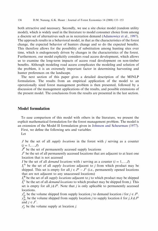
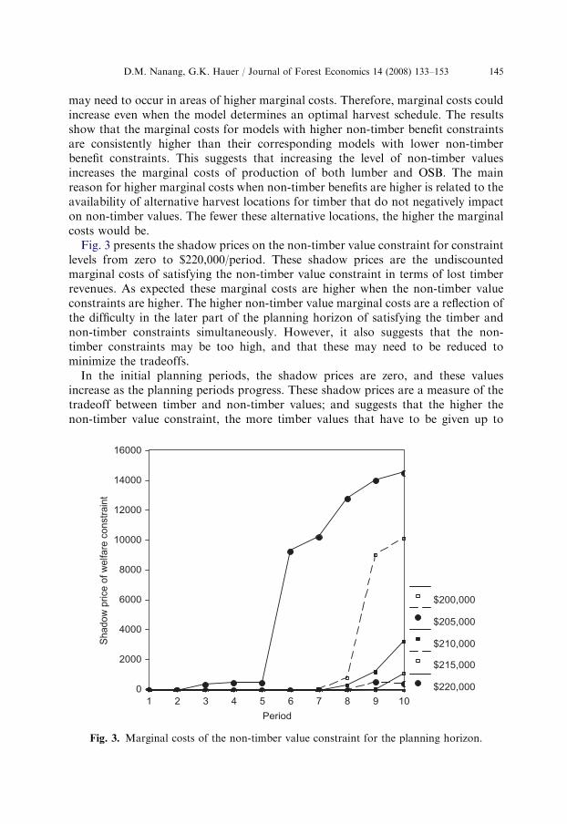
Fig. 3 presents the shadow prices on the non-timber value constraint for constraintlevels from zero to $220,000/period. These shadow prices are the undiscountedmarginal costs of satisfying the non-timber value constraint in terms of lost timberrevenues. As expected these marginal costs are higher when the non-timber valueconstraints are higher. The higher non-timber value marginal costs are a reflection ofthe difficulty in the later part of the planning horizon of satisfying the timber andnon-timber constraints simultaneously. However, it also suggests that the non-timber constraints may be too high, and that these may need to be reduced tominimize the tradeoffs.

In the initial planning periods, the shadow prices are zero, and these valuesincrease as the planning periods progress. These shadow prices are a measure of thetradeoff between timber and non-timber values; and suggests that the higher thenon-timber value constraint, the more timber values that have to be given up to

Period

10987654321

Shadow

price

of w

elfa

re c

onst

rain

t

16000

14000

12000

10000

8000

6000

4000

2000

0

$200,000

$205,000

$210,000

$215,000

$220,000

Fig. 3. Marginal costs of the non-timber value constraint for the planning horizon.

ARTICLE IN PRESS


satisfy the non-timber constraint. For hunting benefits of $220,000, the effect of theconstraint is observed in period 2, whilst for all other constraints less than this value,the effects are not observed until the 7th period and beyond.

Impact of non-timber benefits on harvest schedule

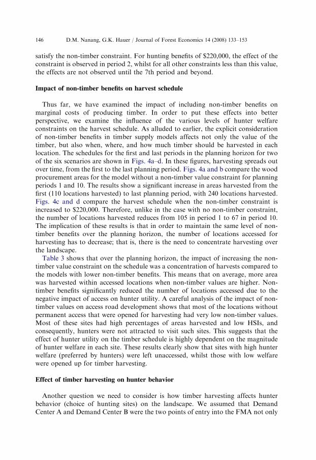
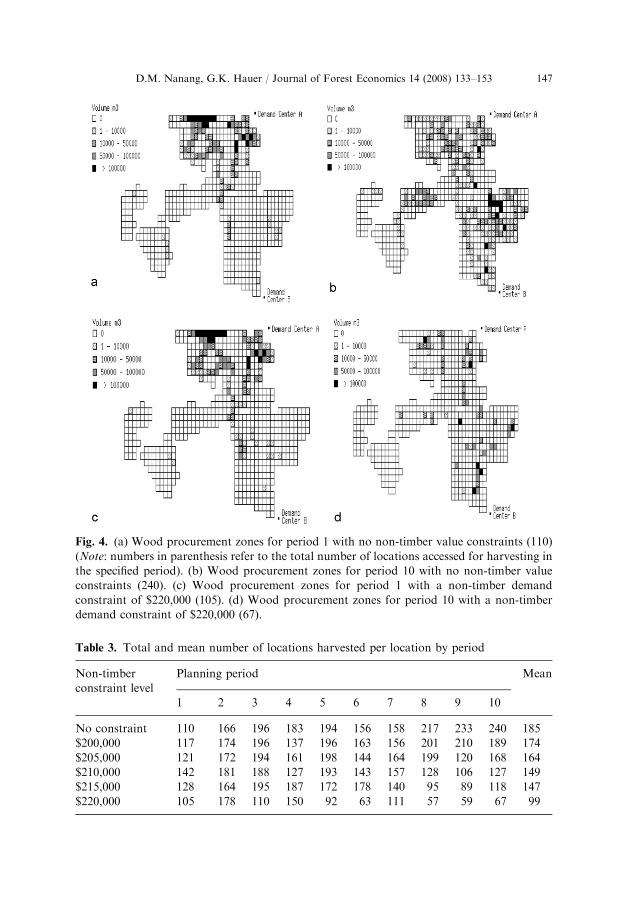
Thus far, we have examined the impact of including non-timber benefits onmarginal costs of producing timber. In order to put these effects into betterperspective, we examine the influence of the various levels of hunter welfareconstraints on the harvest schedule. As alluded to earlier, the explicit considerationof non-timber benefits in timber supply models affects not only the value of thetimber, but also when, where, and how much timber should be harvested in eachlocation. The schedules for the first and last periods in the planning horizon for twoof the six scenarios are shown in Figs. 4a–d. In these figures, harvesting spreads outover time, from the first to the last planning period. Figs. 4a and b compare the woodprocurement areas for the model without a non-timber value constraint for planningperiods 1 and 10. The results show a significant increase in areas harvested from thefirst (110 locations harvested) to last planning period, with 240 locations harvested.Figs. 4c and d compare the harvest schedule when the non-timber constraint isincreased to $220,000. Therefore, unlike in the case with no non-timber constraint,the number of locations harvested reduces from 105 in period 1 to 67 in period 10.The implication of these results is that in order to maintain the same level of non-timber benefits over the planning horizon, the number of locations accessed forharvesting has to decrease; that is, there is the need to concentrate harvesting overthe landscape.

Table 3 shows that over the planning horizon, the impact of increasing the non-timber value constraint on the schedule was a concentration of harvests compared tothe models with lower non-timber benefits. This means that on average, more areawas harvested within accessed locations when non-timber values are higher. Non-timber benefits significantly reduced the number of locations accessed due to thenegative impact of access on hunter utility. A careful analysis of the impact of non-timber values on access road development shows that most of the locations withoutpermanent access that were opened for harvesting had very low non-timber values.Most of these sites had high percentages of areas harvested and low HSIs, andconsequently, hunters were not attracted to visit such sites. This suggests that theeffect of hunter utility on the timber schedule is highly dependent on the magnitudeof hunter welfare in each site. These results clearly show that sites with high hunterwelfare (preferred by hunters) were left unaccessed, whilst those with low welfarewere opened up for timber harvesting.

Effect of timber harvesting on hunter behavior

Another question we need to consider is how timber harvesting affects hunterbehavior (choice of hunting sites) on the landscape. We assumed that DemandCenter A and Demand Center B were the two points of entry into the FMA not only

ARTICLE IN PRESS

Table 3. Total and mean number of locations harvested per location by period

Non-timber

constraint level

Planning period Mean

1 2 3 4 5 6 7 8 9 10

No constraint 110 166 196 183 194 156 158 217 233 240 185

$200,000 117 174 196 137 196 163 156 201 210 189 174

$205,000 121 172 194 161 198 144 164 199 120 168 164

$210,000 142 181 188 127 193 143 157 128 106 127 149

$215,000 128 164 195 187 172 178 140 95 89 118 147

$220,000 105 178 110 150 92 63 111 57 59 67 99

Fig. 4. (a) Wood procurement zones for period 1 with no non-timber value constraints (110)

(Note: numbers in parenthesis refer to the total number of locations accessed for harvesting in

the specified period). (b) Wood procurement zones for period 10 with no non-timber value

constraints (240). (c) Wood procurement zones for period 1 with a non-timber demand

constraint of $220,000 (105). (d) Wood procurement zones for period 10 with a non-timber

demand constraint of $220,000 (67).


ARTICLE IN PRESS


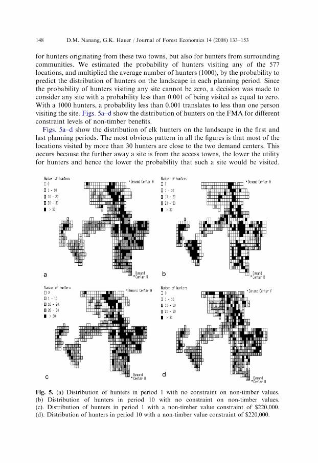
for hunters originating from these two towns, but also for hunters from surroundingcommunities. We estimated the probability of hunters visiting any of the 577locations, and multiplied the average number of hunters (1000), by the probability topredict the distribution of hunters on the landscape in each planning period. Sincethe probability of hunters visiting any site cannot be zero, a decision was made toconsider any site with a probability less than 0.001 of being visited as equal to zero.With a 1000 hunters, a probability less than 0.001 translates to less than one personvisiting the site. Figs. 5a–d show the distribution of hunters on the FMA for differentconstraint levels of non-timber benefits.

Figs. 5a–d show the distribution of elk hunters on the landscape in the first andlast planning periods. The most obvious pattern in all the figures is that most of thelocations visited by more than 30 hunters are close to the two demand centers. Thisoccurs because the further away a site is from the access towns, the lower the utilityfor hunters and hence the lower the probability that such a site would be visited.

Fig. 5. (a) Distribution of hunters in period 1 with no constraint on non-timber values.

(b) Distribution of hunters in period 10 with no constraint on non-timber values.

(c). Distribution of hunters in period 1 with a non-timber value constraint of $220,000.

(d). Distribution of hunters in period 10 with a non-timber value constraint of $220,000.

ARTICLE IN PRESS


The figures reveal several important patterns regarding the distribution of hunters inspace and time on the landscape:

When there is no constraint on non-timber benefits, as in Figs. 5a and b, the totalnumber of locations visited by hunters decreases over time, with the highest numberof locations in period 1 and the least in period 10. This is a direct consequence of thespreading out of timber harvesting from the first to the last period. Increased timberharvesting tends to concentrate hunters to fewer, unaccessed locations. This meansthat when there is less timber harvesting, the hunters are more spread out and whenthere is more timber harvesting they tend to concentrate in the unaccessed areas.

However, when the non-timber value constraint is set at $220,000 as in Figs. 5cand d, the distribution of hunters over the landscape remains relatively unchanged inall planning periods. This distribution is achieved at the expense of reduced numberof locations accessed for harvesting over the planning horizon.

Discussion

The modeling approach and results presented in this paper have severalmanagement applications. First, the models provide shadow price information onthe demand constraints for lumber and OSB. These constraints represent themarginal costs (or marginal values) of production of these two timber outputs. Allmarginal costs for lumber increase with time, indicating scarcity of conifer as wood isharvested off the land base. The significance of these shadow prices is that theyprovide a way of tying the wood production to marginal costs and values of timberand non-timber, which can be compared to expectations of future timber prices. Themodel further provides shadow price (marginal cost) information for non-timbervalue constraint. These marginal costs increase with both time and magnitude of theconstraint level. This increase in marginal costs over time is related to the fact thattimber harvesting spreads out over time and hence non-timber values would decreaseover time without a non-timber value constraint. Once a constraint is imposed toensure the non-timber values do not decrease over time, more timber values have tobe given up to provide the desired level of non-timber values. The implication is thatthe competition between timber and non-timber values may be low in the presentand near future, but would become more acute in the long run.

In this model, three specific factors were found to be significant determinants ofhunter behavior. These were: the percentage of the area harvested in the last 10 yearsin each location, availability or absence of access roads, and the HSI. Bymanipulating these variables, the characteristics of the forest change and so doesthe behavior of hunters regarding which sites they visit. An important policyimplication of these findings is that there appears to be timber managementstrategies that minimize the impact of timber activities on hunters. Similarly, theremay equally be opportunities for influencing hunter behavior that can accommodatea wider scope of timber management. For example, by strategically locating roadaccess and harvesting patterns, forest managers can influence the preference ofhunters for hunting sites, and hence their distribution over the landscape. This is very

ARTICLE IN PRESS


useful in forest planning that seeks to jointly produce timber and non-timberbenefits. For example, if the idea is to zone the forest, it should be possible to createconditions that increase hunter utility in zones specifically designed for hunters. Onthe other hand, by analyzing various harvest levels and number of hunters expectedto visit the FMA, the forest manager can predict where the hunters might be visitingand then reduce harvest activities in such areas.

Another important application of the results presented here is that the model canbe used to understand and analyze the tradeoffs inherent in the joint production oftimber and non-timber values on the same landscape. Restricting timber harvestingto the most valuable stands and concentrating forest management activities in theseareas may serve to reduce the margin of tradeoff between timber and non-timbervalues. This means that timber growing on unaccessed low productivity sites willhave more value if left for non-timber purposes than harvested uneconomically. Thebenefits of doing this is an improvement in timber values by reducing the roadbuilding costs, and increase non-timber values by reducing the negative impacts ofaccess roads on non-timber values.

Although our model has been successful at incorporating non-timber values usingthe RUM, there are still some barriers that have to be cleared before more accurateestimates of non-timber values using this technique can be achieved. First, most sitechoice models operate on very large scales that do not correspond to the spatialscales of forest management. Therefore, for the models to adequately predict theimpacts of forestry activities on hunting behavior, we need to develop recreationmodels that operate at finer scales. Though not implemented, it would have beenpossible in our model to use a landscape unit for hunters that is different from theunit for access. For example, we could have used a township as the unit of analysisfor hunters and still use 1/9th of a township as an access unit. If this were done, itwould allow the use of percentage access as a variable in the random utility model.

It is worthy to caution that the optimal harvest and access schedules that result fromincorporating non-timber values into the timber management plan will undoubtedlydepend on how the variables incorporated in the random utility model affect predictedhunter utility. How variables are included and which variables are left out maysignificantly affect the signs of the coefficients on variables in these models. Forexample, coefficients on road access may be significantly correlated with congestion.Hence, it is important to determine how sensitive harvest and access schedules are todifferences in the variables included in models. In addition, if integrated models such asthe one presented in this paper are to be used in practice, detailed studies of the targetforest management areas are required to find the appropriate site choice model.

Conclusions

This study demonstrates that the decomposition method for solving large-scaleforest management problems introduced by Hoganson and Rose (1984) is aneffective technique for generating acceptable solutions for forest planning modelsinvolving non-timber benefits, in the form of a random utility model. Because the

ARTICLE IN PRESS


model is behavioral, it can be used to analyze the impacts of various levels of timberharvests on non-timber benefits and hunter behavior. Similarly, by using differentlevels of non-timber value constraints, the effects of hunters on the timber values andharvest schedules can be analyzed. A major achievement of this paper is that it hasimproved our understanding of the link between landscape characteristics andchanges and behavioral responses by hunters. By manipulating the main factorsinfluencing hunter behavior, timber management strategies can minimize the impactof timber activities on hunters. Similarly, there are equally opportunities forinfluencing hunter behavior that can accommodate a wider scope of timbermanagement (and reduce multiple-use conflicts), such as growing timber onunaccessed low productive sites that have low hunter benefits. The model can befurther extended to include a feed back in the model for elk populations, and usingfiner spatial scales to estimate the non-timber benefits.

Appendix A. Solution Algorithm

We start with the Lagrangian function for Eqs. (1)–(9), then derive the first-orderconditions.

1.
Assume that zjt ¼ 0, for all JeJP. That is, all non-permanently accessedlocations are initially closed.
2.
Provide initial guesses of timber prices for all tðp0itsÞ 3. For all permanently assessed locations, ðj 2 JPÞ, we calculate the value of wood
at each supply location j. That is: yjt ¼ maxiðpit � csjitÞ (note in the algorithm this

is done for each of six wood products).
4. For all non-permanently assessed locations, jeJP, we defined sub-destinations
on the way to the mills at locations that are permanently accessed and adjacentto areas that are not accessed. The price of wood in each sub-destination iscalculated by solving iteratively the dynamic programming formulation given by

ujt ¼ maxk2IBj

fukt � csjktg þ ljtðzjt � 1Þ, (A.1)

where ljt is the shadow price on the access constraint. This equation says that themarginal value of wood at location j in period t is equal to the maximum of the netvalue of shipping the wood to all adjacent locations minus the shadow cost ofopening the location j if location j is not opened. The equation is solved as follows:

(a) List the supply locations that do not have permanent access according tohow far they are from permanent access. Locations directly adjacent topermanent access are listed first – followed by areas that are one locationaway from permanent access, followed by areas two locations away, etc.

(b) Initialize u0jts for each location to zero.(c) For each time period and location: Solve (A.1) by setting the initial estimates

of ukt to zero. Use the latest update for ljt and zjt. This will give a ujt, and wealso store the best destination (i.e. best supply location).

ARTICLE IN PRESS


(d) Compare this iteration’s u0jts to previous iterations. If they are the same thengo to Step e. Otherwise repeat Step c.

(e) Stop.The u0jts and v0jts (shadow price on Eq. (4) in this formulation are functions ofthe prices we calculate at permanently accessed areas. So there is no iterationprocedure other than the one described above needed to re-estimate theprices. The re-estimate of u0jts are based on re-estimates of p0its.

5.
Assume the p0its are correct and solve the dual (not given) of the primal (Eq. (1))for the remaining dual variables (a0jss and s0jss, the shadow prices for Eqs. (7) and(8), respectively).
6.
Determine the primal solution (the xsjt0s) in Eq. (1) that corresponds to
the optimal dual solution. This primal solution is not necessarily a feasiblesolution.

7.
Determine the output levels for the primal solution found in Step 6 by summingup all flows of wood through a given location in period t. Notice that this flow isnot only from harvest within the associated supply location but also from otherlocations that ship wood through those sub-destinations.
8.
Test for primal feasibility. If the output levels determined in Step 6 are close totheir desired output levels ðys
jtÞ, stop, the primal solution is both an optimal and anear-feasible solution.Otherwise:

9.
Use the output levels determined in Step 7 and a basic understanding of therelationship between output levels and marginal revenue of production to re-estimate the pit values. The p0its were adjusted using the methods presented byHoganson and Rose (1984) and modified by Hauer (1993). Also adjust theshadow prices on the access constraint.
(a) Calculate the approximate value of the shadow price on the access constraintwith ljt as the average cost of opening up a closed location, and cAjt is thefixed cost of accessing a closed location.

(b) Calculate a deviation for this constraint as devjt ¼ ysjt � ys

jtzjt.(c) If devjt ¼ ys

jt � ysjtzjt40, then we adjust l1jt ¼ l0jt;þf ðdevjtÞ

(d) If the devjt ¼ ysjt � ys

jtzjt ¼ 0; ysjt40; zjt ¼ 1; then the price changes are based

on

l1jt ¼ l0jt þ fcAjt

ysjt

� ðbenefit if opened� benefit if closedÞ � l0jt

!.

10.
Update the z0jts. If after the price adjustments above
ljtysjt þ

bt�1

b0

XHh

nhðbenefit if opened� benefit if closedÞXcAjt

then update as zjt ¼ 1 otherwise, zjt ¼ 0.
11. Return to Step 5.

ARTICLE IN PRESS


References

Adamowicz, W.L., Sawit, J., Boxall, P.C., Louviere, J., Williams, M., 1997. Perceptions versus objectivemeasures of environmental quality in combined revealed and stated preference models ofenvironmental valuation. Journal of Environmental Economics and Management 32 (1), 65–84.

Alberta Environment, 2001. Fish and Wildlife Division, Edmonton, Alberta, Canada.Bouzaher, A., Mendoza, G.A., 1987. Goal programming: potential and limitations for agricultural

economists. Canadian Journal of Agricultural Economics 35 (1), 89–107.Buckmaster, G., Todd, M., Smith, K., Bonar, R., Beck, B., Beck, J., Quinlan, R., 1999. Elk winter

foraging habitat suitability index model. Version 5, 8pp.Carter, D.R., Vosiatzis, M., Moss, C.B., Arvanitis, L.G., 1997. Ecosystem management or infeasible

guidelines?: Implications of adjacency restrictions for wildlife habitat and timber production. CanadianJournal of Forest Research 27, 1302–1310.

Diaz-Balteiro, L., Romero, C., 1997. Modeling timber harvest scheduling problems with multiple criteria:an example from Spain. Forest Science 44 (1), 47–57.

Field, D.B., 1973. Goal programming for forest management. Forest Science 19, 125–135.Field, R.C., Dress, P.E., Fortson, J.C., 1980. Complimentary linear and goal programming procedures for

timber harvest scheduling. Forest Science 26, 121–133.Haener, M.K., Adamowicz, W.L., Boxall, P.C., Kuhnke, D., 2001. Aggregation bias in logit models: does

size really matter? unpublished.Harrison, T.P., Rosenthal, R.E., 1986. A multiobjective optimization approach for scheduling timber

harvests on non-industrial private forestlands. In: Systems Analysis in Forestry and Forest Industries.Studies in the Management Sciences 21, 269–283.

Hauer, G.K., 1993. Timber management scheduling with multiple markets and multiple products.Unpublished M.S. Thesis, University of Minnesota.

Hof, J., Raphael, M.G., 1997. Optimization of habitat placement: a case study of the northern spotted owlin the Olympic Peninsula. Ecological Applications 7 (4), 1160–1169.

Hoganson, H.M., Rose, D.W., 1984. A simulation approach to optimal timber management scheduling.Forest Science 30 (1), 220–238.

Johnson, K.L., Scheurman, H.L., 1977. Techniques for prescribing optimal timber harvest and investmentunder different objectives – discussion and Synthesis. Forest Science Monograph 18, 31pp.

Kangas, J., Pukkala, T., 1996. Operationalization of biological diversity as a decision objective in tacticalforest planning. Canadian Journal of Forest Research 26, 103–111.

Kilkki, P., Lappi, J., Siitonen, M., 1986. Long-term timber production planning via utility maximization.In: Systems Analysis in Forestry and Forest Industries. Studies in the Management Sciences 21,285–295.

Kao, C., Brodie, J.D., 1979. Goal programming for reconciling economic, even flow and regulationobjectives in forest scheduling. Canadian Journal of Forest Research 9, 525–531.

Lichtenstein, M.E., Montgomery, C.A., 2003. Biodiversity and timber in the Coast Range of Oregon:inside the production possibility frontier. Land Economics 79 (1), 56–73.

Montgomery, C.A., Pollack, R.A., Freemark, K., White, D., 1999. Pricing biodiversity. Journal ofEnvironmental Economics and Management 38, 1–19.

Nalle, D.J., Montgomery, C.A., Arthur, J.L., Polasky, S., Schumaker, N.H., 2004. Journal ofEnvironmental Economics and Management 48, 997–1017.

Nelson, J.D., Shannon, T., Errico, D., 1993. Determining the effects of harvesting guidelines on the age-class profile of the residual forest. Canadian Journal of Forest Research 23, 1870–1880.

Teeguarden, D.E., 1982. Multiple services. In: Duerr, W.A., Teeguarden, D.E., Christiansen, N.B.,Guttenberg, S. (Eds.), Forest Resource Management: Decision-making Principles and Cases. Corvallis,Oregon, pp. 276–290.

integrating a random utility model for non-timber forest users into a strategic forest planning...

Documents