influence of global correlations on central limit theorems and entropic extensivity
TRANSCRIPT

1/25
Influence of global correlations on central limit theorems and entropic extensivity
John A. Marsh1, Miguel A. Fuentes2,3,
Luis G. Moyano4 and Constantino Tsallis2,4
1SI International, 7900 Turin Road, Rome, NY 13440, USA 2Santa Fe Institute, 1399 Hyde Park Road, Santa Fe, NM 87501, USA 3Consejo Nacional de Investigaciones Científicas y Técnicas, Centro
Atómico Bariloche and Instituto Balseiro, 8400 Bariloche, Rio Negro, Argentina 4Centro Brasileiro de Pesquisas Físicas, Rua Xavier Sigaud 150, 22290-180
Rio de Janeiro, Brazil
Abstract We consider probabilistic models of N identical distinguishable, binary
random variables. If these variables are strictly or asymptotically independent, then, for N → ∞ , (i) the attractor in distribution space is, according to the standard central limit theorem, a Gaussian, and (ii) the Boltzmann-Gibbs-
Shannon entropy 1
lnW
BGS i iiS p p
=≡ −∑ (where W = 2N) is extensive, meaning
that SBGS(N) ~ N . If these variables have any nonvanishing global (i.e., not asymptotically independent) correlations, then the attractor deviates from the Gaussian. The entropy appears to be more robust, in the sense that, in some cases, SBGS remains extensive even in the presence of strong global correlations. In other cases, however, even weak global correlations make the entropy deviate from the normal behavior. More precisely, in such cases the entropic form
( )11 1
1W q
q iq iS p− =
≡ −∑ (with 1 BGSS S≡ ) can become extensive for some value of
1q ≠ . This scenario is illustrated with several new as well as previously described models. The discussion illuminates recent progress into q-describable nonextensive probabilistic systems, and the conjectured q-Central Limit Theorem (q-CLT) which posses a q-Gaussian attractor.
1. Introduction
The foundation of statistical mechanics is a probabilistic description of macroscopic systems reflecting microscopic dynamical behavior. If the assumption of ergodicity holds in configurational phase space, then we have standard Boltzmann-Gibbs statistical mechanics. Chaos theory provides the basic tools and simple models to study situations in which ergodicity may be violated, showing fractal, hierarchical, or other incomplete occupation of phase space. A generalization of the Boltzmann-Gibbs-Shannon entropy SBGS may provide a fundamental description characterized by a single real parameter q. The entropy Sq is defined, for a system with W microstates with occupation probabilities pi , as follows:

2/25
1
11
1
Wq
q ii
S pq =
⎛ ⎞≡ −⎜ ⎟− ⎝ ⎠∑ (with 1
1
lnW
BGS i ii
S S p p=
= ≡ −∑ ) (1)
For composition of independent subsystems, where the joint probabilities satisfy a product law, Sq is extensive for q = 1, and nonextensive for 1q ≠ . In many
respects, the appearance of nonextensivity provides an essential description of natural, man-made, and even social phenomena. For example, in physical systems, long-range interactions (and, hence, global correlations) among system components, or long-range memory, imply that the composition of systems cannot proceed using the assumption of probabilistic independence.
The statistical mechanics associated with Sq, which parallels that associated with Boltzmann-Gibbs entropy, has been developed to a considerable degree [1], and gives rise to the so-called nonextensive statistical mechanics, with stationary state distribution function showing power-law (“heavy-tail”) decay. Strong connections have also been made by Robledo and collaborators [2] (see also [3]) between the q-statistical concepts and nonlinear dynamical systems such as unimodal one-dimensional maps at the edge of chaos and elsewhere.
Recent developments [4,5] have provided a number of simple examples which illustrate the interconnected nature of these concepts and the applicability of this formalism to natural systems, in which strongly correlated behaviors and power-law distributions are ubiquitous, yet largely unexplained.
The aim of this communication is to explore globally correlated systems composed of N distinguishable and identical random binary variables. Two aspects of these systems are of particular interest: first, the question of extensivity of the entropy Sq, and second, the nature of the attractor in the space of probability distributions. Each of these aspects may show anomalous behavior due to global correlations, in contrast to the more normal behavior associated with strictly or nearly independent system composition. The entropy Sq which is extensive in the case of independence is that with q = 1, whereas the anomalous case shows extensivity for q ≠ 1. Correspondingly, for independent systems, the attractor in probability space is a Gaussian, as studied by A. de Moivre (1733), P.S. de Laplace (1774), R. Adrain (1808) and C.F. Gauss (1809), when the variance of the single distribution is finite. If this variance diverges instead, the attractor is a Levy distribution, as studied by P. Levy and B.V. Gnedenko in the 1930’s. In the anomalous case (i.e., when global correlations are present), a variety of attractors have been conjectured or discussed [6], most notably the q-Gaussian distribution [5,7]. This distribution optimizes the entropy Sq, and so the two anomalous features induced by global correlations are intimately related. Several examples of globally correlated systems will be studied here in this context, and the unified picture that emerges will be discussed in the light of recent progress [5,7] at a q-generalized central limit theorem (q-CLT).
This new formalism has also been shown [8] to yield a fundamental explanation for the emergence of networks in nature: network nodes are interpreted as special points (or regions) in a more-or-less continuous phase space which show non-vanishing occupancy.

3/25
non q-describable
qent = 1
qent ≠ 1
Gaussian attractor
q-describable
non q-describable
qent = 1
qent ≠ 1
Gaussian attractor
q-describable
(A) (B)
present2
present1
MTG
α < 0
TGS2
TGS3
α > 0
α > 0
α < 0
Gaussian attractor
qent = 1
qent ≠ 1
present3
L
TGS1
present2
present1
MTG
α < 0
TGS2
TGS3
α > 0
α > 0
α < 0
Gaussian attractor
qent = 1
qent ≠ 1
present3
L
TGS1non q-describable
qent = 1
qent ≠ 1
Gaussian attractor
q-describable
non q-describable
qent = 1
qent ≠ 1
Gaussian attractor
q-describable
(A) (B)
present2
present1
MTG
α < 0
TGS2
TGS3
α > 0
α > 0
α < 0
Gaussian attractor
qent = 1
qent ≠ 1
present3
L
TGS1
present2
present1
MTG
α < 0
TGS2
TGS3
α > 0
α > 0
α < 0
Gaussian attractor
qent = 1
qent ≠ 1
present3
L
TGS1
Fig. 1: (A) Schematic representation of the classes of probabilistic systems discussed. The class of q-describable systems is defined as those for which the entropy Sq is extensive for some q = qent. The q-describable systems are further divided into those for which the Boltzmann-Gibbs-Shannon entropy SBGS = S1 is extensive, and those for which Sq is extensive for 1entq ≠ . The Gaussian attractor occurs for the special case of
independent system composition, and is represented here by a single point contained within the space of qent = 1 q-describable systems. (B) Detail showing the various models discussed in this work, appearing as lines parameterized by some variable in the model. The positioning of the lines indicates whether qent equals unity or differs from unity. The various models are labeled as discussed in the text: the MTG endpoint L represents the Leibnitz triangle.
The simplest setting in which to study correlated behavior of a large number
of subsystems is discrete k-state systems under composition. (We note that analogous constructions can be made for continuous systems [4]). As N k-state systems are composed, the number of possible states is given by W = kN. Let us denote by effW the number of states whose probability is (sensibly) different from zero (eff stands for effective). If the subsystems are independent, then generically eff NW W k= = . If, furthermore, each of these possibilities has probability on the order of 1/ Nk , the BGS entropy is given by
~ ln ~ lnBGSS W N k , and thus shows extensive behavior (i.e., SBGS ~ N
as N → ∞ , or, equivalently, 0 lim q
N
S
N→∞< < ∞ ) only for qent = 1. Thus, the
composition of (strictly or nearly) uncorrelated systems is described by the usual entropy. However, if strong correlations exist among subsystems, then, in general, many microstates of the system might be forbidden. For a large class of interesting systems, the effective number of states
~ ( 0)eff NW N W kρ ρ<< = > , in which case

4/25
( )1
1( ) 1~ ln ~
1
eff qqeff
q q
WS W N
qρ
−−−≡
−. (2)
In this case Sq is extensive for and only for
1
1entqρ
= − . (3)
This simple argument links a (appreciably) reduced occupancy of phase space, corresponding to a breaking of ergodicity, with the entropy Sq and the associated nonextensive theory. It becomes clear now that the expression “nonextensive entropy” sometimes used for Sq, is appropriate only for “normal” systems (i.e., those constituted by subsystems which are mutually independent), not in general. For such systems, the multiplicity of microstates is exponential in the number N of composed subsystems. Focus has now turned instead to the so-called “q-describable” systems [4, 9] in which the entropy Sq shows extensive behavior for some qent equal to or different from unity. Fig. 1a shows a schematic representation of these possibilities, with q-describable systems forming a subset of all possible systems, and q-describable systems with qent = 1 forming a further subset of the q-describable systems. The “normal”, or independent, case is shown as a point located at the boundary of the qent = 1 and
1≠entq regions of the q-describable systems. We will return to Fig. 1 in the next section, when specific models are discussed.
r20 r21 r22
r30 r31 r32 r33
r10 r11
N = 3
N = 2
N = 1
r20 r21 r22
r30 r31 r32 r33
r10 r11
r20 r21 r22
r30 r31 r32 r33
r10 r11
N = 3
N = 2
N = 1
Fig. 2: Pascal-Leibnitz triangle configuration of reduced probabilities rN,n illustrated for number of composed systems N = 1, 2, 3.
Our interest here lies not only in simple examples of q-describable systems,
but also some indications as to whether q-statistics (with the associated power-law generalizations of the natural logarithm and exponential functions) constitutes a fundamental explanation of (asymptotic) scaling and power-law behavior observed so often in nature. Optimizing Sq in the new formalism, with appropriate constraints, yields the so-called q-Gaussian, a generalized form of
the Gaussian distribution, given by ( ) 2
e xqf x β−∝ , where β characterizes the
width, and the q-exponential function ( ) ( )1 11 1
qxqe q x
−≡ + −⎡ ⎤⎣ ⎦ (so defined where

5/25
( )1 1 0q x− − > , and 0 elsewhere) appears, and reduces, as expected, to the usual
exponential function in the limit q = 1. This q-Gaussian distribution has power law tails for 1 < q < 3, has compact support for q < 1, and recovers the usual Gaussian distribution for q = 1. From this perspective, we expect the q-Gaussian to appear often in nature, associated with strongly correlated complex systems. Indeed, a considerable amount of evidence exists today for the ubiquitous nature of power-law behavior in both natural and man-made systems, and the possibility that the q-statistical formalism is in some sense fundamental in nature is thus very appealing.
Important evidence in support of such a possibility has recently appeared in the form of numerical indications [5, 7], and a formal development of a q-qeneralized Central Limit Theorem (q-CLT) is in progress.
A natural starting point is the case of identical and distinguishable binary subsystems, but which are not necessarily independent. We let p denote the probability that the binary system is in state 0, out of a state space { }0,1 . When
N such systems are composed, the full state space may be considered to consist of all 2N possible binary strings of length N. Because the systems are identical, these 2N probabilities can be reduced to just N values ,N nr , each with
multiplicity given by the binomial coefficient ( )! ! !N N n n−⎡ ⎤⎣ ⎦ , where n = 0,
1, … , N. These reduced probabilities ,N nr thus satisfy the normalization
condition
( ) ,
0
!1
! !
N
N nn
Nr
N n n==
−∑ (4)
and ,N nr can be thought of as counting the number of subsystems in the state 1
(and thus 1,0r p≡ and 1,1 1r p≡ − ). Any specific prescription for successively
adding binary systems to the N-system yields a sequence of systems, whose reduced probabilities ,N nr can be arranged into a triangle, as shown in Fig. 2. The
corresponding arrangement of the binomial coefficients is the familiar Pascal triangle. Since each of the N single random variables can take values 0 or 1, the index n corresponds to the value of the random variable defined by the sum of all N binary random variables. Therefore, the attractors that emerge after centering and rescaling n, precisely correspond to the natural abscissa associated with all central limit theorems. The abscissa n measured from its "center" (value of n, for given N, for which pN,n is maximal) scales, in all the models that we discuss in the present paper, as Nγ with 0γ ≥ . Therefore, 1
2γ =

6/25
n (centered)
N
log(rN,n)
(A)20 40 60 80 100
20
40
60
80
100
-60
-50
-40
-30
-20
-10
n (centered)
N
log(pN,n)
(B)20 40 60 80 100
20
40
60
80
100
-60
-50
-40
-30
-20
-10
0 100 200 300 4000
0.02
0.04
0.06
0.08
0.1
0.12
n
pN
,n
(C)0 100 200 300 400
10-150
10-100
10-50
100
n
pN
,n
(D)
N = 100
N = 200
N = 300
N = 400
-2 0 20
0.2
0.4
0.6
0.8
(n - N/2)/N0.5
N0.
5 pN
,n
(E)-10 -5 0 5 10
10-150
10-100
10-50
100
(n - N/2)/N0.5
N0.
5 pN
,n
(F)
N = 100
N = 200
N = 300
N = 400
Fig. 3: Behavior of independent binary system composition for the case p = 0.5. Each model discussed in this paper has this case as a limiting case. Parts (A)-(B) show reduced probabilities log(rN,n) and probabilities log(pN,n) up to N = 100 as grayscale images. Parts (C)-(D) show uncentered and unscaled probabilities for N = 50, 100, … , 400, in both linear and log units. Parts (E)-(F) show centered and scaled probabilities, illustrating the Gaussian attractor in probability space.
corresponds to normal diffusion, 1
2γ > corresponds to superdiffusion, and 120 γ≤ < corresponds to subdiffusion (γ = 0 means in fact localization).
A scale-invariant construction, yielding systems suitable for analysis in the thermodynamic limit N → ∞ , can be imposed by requiring the marginal probabilities of the system at level N in the construction to reproduce the joint probabilities at level N - 1. It can be verified that this condition is equivalent to imposing the Leibnitz rule for the reduced probabilities: , , 1 1,N n N n N nr r r+ −+ = .
7/25
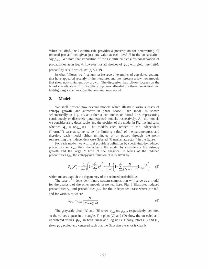
When satisfied, the Leibnitz rule provides a prescription for determining all reduced probabilities given just one value at each level N in the construction, say ,0Np . We note that imposition of the Leibnitz rule ensures conservation of
probabilities as in Eq. 4, however not all choices of ,0Np will yield admissible
probability sets in which 0 1,ip i≤ ≤ ∀ . In what follows, we first summarize several examples of correlated systems
that have appeared recently in the literature, and then present a few new models that show non-trivial entropy growth. The discussion that follows focuses on the broad classification of probabilistic systems afforded by these considerations, highlighting some questions that remain unanswered.
2. Models
We shall present now several models which illustrate various cases of entropy growth, and attractor in phase space. Each model is shown schematically in Fig. 1B as either a continuous or dotted line, representing continuously or discretely parameterized models, respectively. All the models we consider are q-describable, and the position of the model in Fig. 1A indicates whether 1=entq or 1≠entq . The models each reduce to the independent (“normal”) case at some value (or limiting value) of the parameter(s), and therefore each model either terminates at or passes through the point representing the independent case (labeled “Gaussian attractor”) in the figure.
For each model, we will first provide a definition by specifying the reduced probability set rN,n, then characterize the model by considering the entropy growth and the large N limit of the attractor. In terms of the reduced probabilities rN,n, the entropy as a function of N is given by
( ) ( ) ( )2
,1 0
1 1 !1 1
1 1 ! !
N Nqq
q i N ni n
NS N p r
q q N n n= =
⎛ ⎞⎛ ⎞≡ − = −⎜ ⎟⎜ ⎟ ⎜ ⎟− − −⎝ ⎠ ⎝ ⎠
∑ ∑ , (5)
which makes explicit the degeneracy of the reduced probabilities. The case of independent binary system composition will serve as a model
for the analysis of the other models presented here. Fig. 3 illustrates reduced probabilities nNr , and probabilities pN,n for the independent case where p = 0.5,
and for various N, where
( ), ,
!
! !N n N n
Np r
N n n≡
−. (6)
The grayscale plots (A) and (B) show nNr , and nNp , , respectively, centered
so the values appear in a triangle. The plots (C) and (D) show the unscaled and uncentered values nNp , in both linear and log units. Finally, plots (E) and (F)
show nNp , scaled and centered such that the Gaussian attractor is clearly

8/25
n (centered)
N
log(rN,n)
(A)20 40 60 80 100
20
40
60
80
100 -70
-60
-50
-40
-30
-20
-10
0
n (centered)
N
log(pN,n)
(B)20 40 60 80 100
20
40
60
80
100 -12
-10
-8
-6
-4
-2
0
0 20 40 60 80 1000
0.02
0.04
0.06
0.08
n
pN
,n
(C)
0 20 40 60 80 10010
-5
10-4
10-3
10-2
10-1
pN
,n
n(D)
N = 40
N = 60
N = 80
N = 100
-1 -0.5 0 0.5 10
0.5
1
1.5
x = (n - ncenter)/Nγ
Nγ
p N,n
(E)-1 -0.5 0 0.5 1
10-4
10-3
10-2
10-1
100
x = (n - ncenter)/Nγ
Nγ
p N,n
(F)
Fig. 4: The behavior of the MTG model with parameter qcorr = 0.8. Parts (A)-(B) show reduced probabilities log(rN,n) and probabilities log(pN,n) up to N = 100 as grayscale images. Parts (C)-(D) show uncentered and unscaled probabilities for N = 30, 40, … , 100, in both linear and log units. Parts (E)-(F) show centered and scaled probabilities, illustrating the attractor in probability space. We find γ = 0.88.
observed. Indeed, as seen in the axis labels, the scaling makes use of the fact that the centers of the unscaled distributions occur at values N/2, and the widths scale
as N . In general, for the models presented here, the attractor in phase space is scaled by first centering, and then applying the rule
( ), ,N n N n
center
p p N
n nn
N
γ
γ
→
−→
, (7)

9/25
which generalizes the scaling used for the independent (Gaussian) case, where the exponent was 5.0=γ . The exponent γ characterizes the diffusion rate of the
random process.
2.1 A q-describable model with qent = 1 and a q-Gaussian attractor
We consider first the model referred to as MTG in Fig. 1, that has provided [5] numerical evidence for a generalized central limit theorem. The construction works in analogy to the case of independent subsystem composition, where ,0 1,0
N NNr r p= ≡ . Application of the Leibnitz rule then yields the usual
form ( ), 1nN n
N nr p p−= − . Global correlations can be introduced through the q-
product [10], defined as follows
( ) ( )1
1 1 111q q q
qx y x y x y xy− − −⊗ ≡ + − ⊗ = , (8)
where it is required that , 1x y ≥ , and 1q ≤ . From this definition, the form
N
nN pr ⎟⎟⎠
⎞⎜⎜⎝
⎛= 11
,
, (9)
valid for independent subsystem composition, is generalized to
( )1
11 1
,0
1 1 11corr corr
corr corr corr
q qN q q qr Np N
p p p
−
− −⎡ ⎤⎛ ⎞ ⎛ ⎞ ⎛ ⎞ ⎡ ⎤= ⊗ ⊗ ⊗ = − −⎢ ⎥⎜ ⎟ ⎜ ⎟ ⎜ ⎟ ⎣ ⎦⎝ ⎠ ⎝ ⎠ ⎝ ⎠⎣ ⎦
(10)
where corr stands for correlation. The case 1corrq = yields the independent case, as the q-product reduces to the usual product when q = 1. And the case
0corrq = and 0.5p = yields ( ) 1
,0 1Nr N−= + , which is the original Leibnitz
triangle construction [11]. The MTG model is illustrated in Figs. 4-5 for qcorr = 0.8, and 0.3, respectively.
With the rN,0 specified as in Eq. 10 above, the Leibnitz rule is applied to define the remaining reduced probabilities. As discussed in more detail in the original reference [5], this model reproduces, in the limit N → ∞ , a q-generalization of the de Moivre-Laplace version of the Central Limit Theorem. Indeed, the probability distribution closely approaches a q-Gaussian,
( ) 2
e xQp x β−∝ , (11)

10/25
n (centered)
N
log(rN,n)
(A)20 40 60 80 100
20
40
60
80
100 -70
-60
-50
-40
-30
-20
-10
0
n (centered)
N
log(pN,n)
(B)20 40 60 80 100
20
40
60
80
100 -6
-5
-4
-3
-2
-1
0
0 20 40 60 80 1000
0.01
0.02
0.03
0.04
0.05
n
pN
,n
(C)
0 20 40 60 80 10010
-3
10-2
10-1
pN
,n
n(D)
N = 40
N = 60
N = 80
N = 100
-1 -0.5 0 0.5 10.2
0.4
0.6
0.8
1
1.2
x = (n - ncenter)/Nγ
Nγ p
N,n
(E)-1 -0.5 0 0.5 1
0.4
0.6
0.8
1
x = (n - ncenter)/Nγ
Nγ
p N,n
(F)
Fig. 5: The behavior of the MTG model with parameter qcorr = 0.30. Parts (A)-(B) show reduced probabilities log(rN,n) and probabilities log(pN,n) up to N = 100 as grayscale images. Parts (C)-(D) show uncentered and unscaled probabilities for N = 30, 40, … , 100, in both linear and log units. Parts (E)-(F) show centered and scaled probabilities, illustrating the attractor in probability space. We find γ = 0.96.
except for a very small amount of asymmetry. The relation between the original qcorr supplied to the construction (via the q-product of Eq. 10), and the value Q that characterizes the limiting q-Gaussian distribution function is quite simple, and obtained numerically [5] as 2 1 corrQ q= − .

11/25
0 10 20 30 40 50-70
-60
-50
-40
-30
-20
-10
0
Nmax = 80, 100
(n - N/2)/Nγ)2
lnQ
(pN
,n/p
N,n
max
)
qcorr = 1
Q = 2 - 1/qcorr = 1
(A)
qcorr = 1
Q = 2 - 1/qcorr = 1
(A)
N = 80
N = 100
0 1 2 3 4 5-8
-7
-6
-5
-4
-3
-2
-1
0
Nmax = 100
(n - N/2)/Nγ)2
lnQ
(pN
,n/p
N,n
max
)
qcorr = 0.9
Q = 2 - 1/qcorr = 0.89
(B)
0 0.5 1 1.5 2 2.5 3-4
-3.5
-3
-2.5
-2
-1.5
-1
-0.5
0
Nmax = 100
(n - N/2)/Nγ)2
lnQ
(pN
,n/p
N,n
max
)
qcorr = 0.8
Q = 2 - 1/qcorr = 0.75
(C)0 0.2 0.4 0.6 0.8 1 1.2 1.4
-0.35
-0.3
-0.25
-0.2
-0.15
-0.1
-0.05
0
Nmax = 100
(n - N/2)/Nγ)2
lnQ
(pN
,n/p
N,n
max
)
qcorr = 0.25
Q = 2 - 1/qcorr = -2
(D) Fig. 6: The probabilities pN,n for the MTG model, replotted to illustrate the approach to the q-Gaussian form. (A) qcorr = 1.0, where the deviation from a straight line is a finite-size effect, also apparent in Fig. 3F, and is illustrated using two N values, (B) qcorr = 0.9, (C) qcorr = 0.8, as shown in Fig. 4, (D) qcorr = 0.25, similar to the case shown in Fig. 5. In each case the Q-log of the probabilities, with the appropriate Q, is plotted as a function of scaled n2, showing a straight line, in agreement with the q-Gaussian form.
Figure 6 illustrates the q-Gaussian attractor explicitly by plotting the q-log
of the probability set vs. the square of the centered index centernn − , which
yields a straight line for q-Gaussian distributions. Indeed, for the independent case of Fig. 3, where qcorr = 1, and the various qcorr values of Fig. 6, we find good numerical agreement with the equation 2 1 corrQ q= − . The slight asymmetry noted in Ref. [5] is also apparent in Fig. 6B-D.
The correlations introduced into this model are, although global in nature, relatively weak, and the model exhibits qent = 1 for all values of qcorr. This may be expected, since Weff ~ 2N. Figure 7 shows an example of Sq vs. N for qcorr = 0.25, demonstrating that qent = 1.
2.2 A q-describable model with qent = 1, and non-q-Gaussian attractor
We consider next a generalization of the independent system case, referred to as TGS1 in Fig. 1, which has appeared previously in Ref. [4]. This model is defined using a stretched exponential as follows
,0 1,0N N
Nr r pα α
= = , (12)

12/25
where α is a parameter constrained to the range [0, 1] (for α outside this range, some of the rN,n become unphysical). The other reduced probabilities are constructed using the Leibnitz rule. At one extreme, α = 0, only two values, rN,0 and rN,N are nonzero. The opposite extreme, α = 1 reduces to the independent case (Gaussian attractor). Figure 8 illustrates the behavior of this model for case α = 0.9.
0 5 10 15 20 250
5
10
15
20
25
N
Sq
q = 0.6 q = 0.7
q = 0.8
q = 0.9
q = 1.0
q = 1.1
q = 1.2
Fig. 7: Entropy growth in the model “MTG” defined in Eq. 10, for the case qcorr = 0.25, showing that SBGS is extensive (i.e., qent = 1).
The attractor clearly deviates from the Gaussian, however for the entire
range of α this model exhibits extensive qent = 1. In Fig. 1B, this model thus resides in the qent = 1 region of the q-describable systems, and terminates at the Gaussian attractor, thus providing a second example of a system for which the attractor deviates from the Gaussian, yet the correlations are not strong enough to give 1≠entq .
2.3 Two q-describable models with qent ≠ 1, and non-q-Gaussian attractor
We consider next a q-describable model [4] for which 1entq ≠ . This model is referred to as model TGS2 in Fig. 1B, and is shown as a series of dots, since the model is discretely parameterized. The model is based on restricted occupancy, such that the effective occupancy ~eff dW N for some positive integer d. The reduced probabilities are specified as
( )
1min( , )
, 0
1 !
! !
0 otherwise
d N
effN n k
Nn d
r N k kW
−
=
⎧ ⎛ ⎞⎪ = ≤⎜ ⎟⎜ ⎟= −⎨ ⎝ ⎠⎪⎩
∑ . (13)

13/25
n (centered)
N
log(rN,n)
(A)20 40 60 80
20
40
60
80
100-50
-40
-30
-20
-10
0
n (centered)
N
log(pN,n)
(B)20 40 60 80
20
40
60
80
100 -25
-20
-15
-10
-5
0
0 20 40 60 800
0.05
0.1
0.15
0.2
0.25
n
pN
,n
(C)
0 20 40 60 8010
-15
10-10
10-5
100
pN
,n
n(D)
N = 20
N = 40
N = 60
N = 80
-2 -1 0 1 20
0.2
0.4
0.6
0.8
1
x = (n - ncenter)/Nγ
Nγ p
N,n
(E)-2 -1 0 1 2
10-15
10-10
10-5
100
x = (n - ncenter)/Nγ
Nγ
p N,n
(F)
Fig. 8: Behavior of the model “TGS1”, defined in Eq. 12, for α = 0.9. Parts (A)-(B) show reduced probabilities log(rN,n) and probabilities log(pN,n) up to N = 100 as grayscale images. Parts (C)-(D) show uncentered and unscaled probabilities for N = 10, 20, … , 80, in both linear and log units. Parts (E)-(F) show centered and scaled probabilities, illustrating the attractor in probability space. We find γ = 0.70. In case dN ≤ , the summation extends to k = N, so the probabilities reproduce the case of independent system composition. For N > d, the summation extends only to k = d, yielding non-zero occupation only in the first d+1 reduced probabilities. Note the normalization condition of Eq. 4 is satisfied by this prescription. Figure 9 illustrates the behavior of this model, for the case d = 15.
In the case d N= , this model reduces to the independent case, yielding a Gaussian attractor, and qent = 1. For finite d, the attractor of this model is a delta
14/25
n (centered)
N
log(rN,n)
(A)20 40 60 80 100
20
40
60
80
100 -40
-30
-20
-10
n (centered)
N
log(pN,n)
(B)20 40 60 80 100
20
40
60
80
100 -40
-30
-20
-10
10 12 14 16 18 200
0.2
0.4
0.6
0.8
1
n
pN
,n
(C)
0 5 10 15 2010
-30
10-20
10-10
100
pN
,n
n(D)
N = 50
N = 100
N = 400
N = 50 N = 400
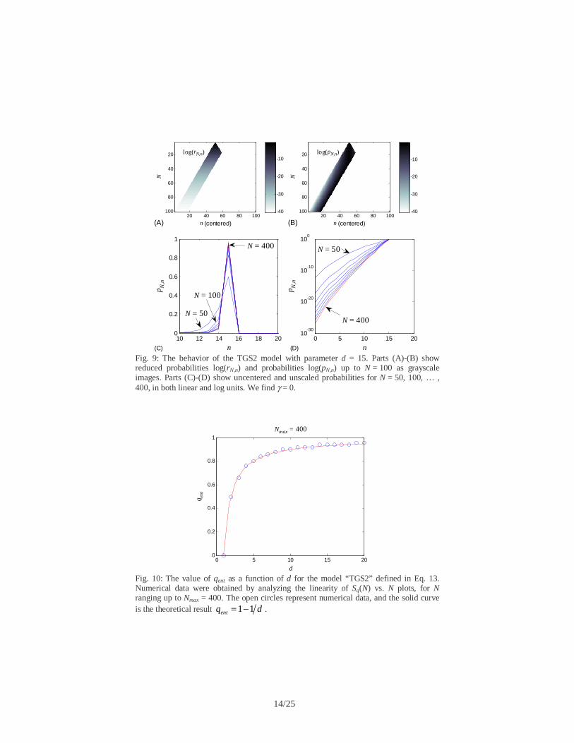
Fig. 9: The behavior of the TGS2 model with parameter d = 15. Parts (A)-(B) show reduced probabilities log(rN,n) and probabilities log(pN,n) up to N = 100 as grayscale images. Parts (C)-(D) show uncentered and unscaled probabilities for N = 50, 100, … , 400, in both linear and log units. We find γ = 0.
0 5 10 15 200
0.2
0.4
0.6
0.8
1
d
Nmax = 400
qen
t
Fig. 10: The value of qent as a function of d for the model “TGS2” defined in Eq. 13. Numerical data were obtained by analyzing the linearity of Sq(N) vs. N plots, for N ranging up to Nmax = 400. The open circles represent numerical data, and the solid curve is the theoretical result dqent 11−= .

15/25
function, clearly deviating from the Gaussian distribution. Furthermore, because [4] the effective number of states Weff ~ Nd, the value of qent satisfies the theoretical form 1 1entq d= − . Figure 10 illustrates this agreement with numerical simulation results, in which the qent was determined in each case by fitting a straight line to the Sq vs. N curves, and maximizing the R2 value of the fit. Figure 11 gives an example of the entropy growth curves for the case d = 5, verifying that qent = 0.8 gives linear entropy growth, as predicted.
0 50 100 150 200 250 300 350 4000
50
100
150
200
250
300
350
400
N
Sq
q = 0.7 q = 0.8
q = 0.9
Fig. 11: Entropy growth for the model TGS2 defined in Eq. 13, for the case d = 5, demonstrating numerically that linear entropy growth is observed for 8.011 =−= dqcorr .
The model TGS2 does not show scale invariance, as the Leibnitz rule is
violated, even asymptotically. However, an asymptotically scale-free variation on this model, using the same cutoff parameter d, has been produced in Ref. [4]. This model is referred to as TGS3 in Fig. 1B, and has similar properties to that of TGS2, being discretely parameterized, exhibiting a similar delta function attractor, and satisfying the same theoretical prediction 1 1entq d= − . Figure 12 illustrates the behavior of this model for the case d = 4.
Both TGS2 and TGS3 provide examples of systems for which the global correlations are so strong that 1≠entq , in addition to the attractor deviating substantially from the Gaussian.
2.4 A new class of q-describable models with qent ≠ 1, and non-q-Gaussian attractor
We introduce now a new class of models which offer further insight into the conditions necessary for 1entq ≠ . Three examples from this class will be presented.
The first example from this new class, referred to as “present1” in Fig. 1B, is defined by the reduced probabilities

16/25
( ),
0
!! !
n
N n Nk
k
Nr
NN
N k k
α
α
=
=
−∑ (14)
where α is a real constant, and the denominator ensures proper normalization. This model introduces correlations so strongly that the probability set at level N does not depend in a simple way on the probability set at level N – 1, and so does not adhere to the Leibnitz rule. The case α = 0 reduces to the independent
n (centered)
N
log(rN,n)
(A)20 40 60 80 100
20
40
60
80
100
-15
-10
-5
0
n (centered)
N
log(pN,n)
(B)20 40 60 80 100
20
40
60
80
100-2.5
-2
-1.5
-1
-0.5
0
0 1 2 3 40
0.1
0.2
0.3
0.4
0.5
n
pN
,n
(C)
0 1 2 3 410
-2
10-1
100
pN
,n
n(D)
N = 30
N = 100
N = 100
N = 30
Figure 12: The behavior of the “TGS3” model with parameter d = 4. Parts (A)-(B) show reduced probabilities log(rN,n) and probabilities log(pN,n) up to N = 100 as grayscale images. Parts (C)-(D) show uncentered and unscaled probabilities for N = 30, 40, … , 100, in both linear and log units. We find γ = 0.
composition case, and so yields qent = 1. However, for 1α ≠ , we find 1entq ≠ .
Indeed, Fig. 13 shows the entropy growth with N for α = -1.0, and for several values of q, demonstrating qent ≈ 0.7. Figure 14 shows the dependence of qent on the parameter α, where each value of qent is determined by maximizing the R2 value from straight line fits to Sq(N) vs N. The model is symmetric in α, as shown. The figure also shows a fit to a stretched q-Gaussian of the form
( )( )41
4 1e 1 1 Qent Qq Qα α− −= = − − , (15)

17/25
0 5 10 15 20 250
5
10
15
20
25
N
Sq
q = 0.4 q = 0.5
q = 0.6
q = 0.7
q = 0.8
q = 0.9 q = 1.0
Fig. 13: Entropy growth for the model “present1” defined in Eq. 14, with parameter α = -1. The entropy growth curves for various q, showing the entropy Sq is extensive for qent ≈ 0.7. where the fitted parameter 5.0Q ≅ . This parameter is found to depend in a systematic way on the maximum value N used in the straight-line fits to Sq(N) vs. N, and is found to closely approach Q = 5.0 as N → ∞ . The asymptotic behavior for large α is thus well-described by the simple form
1~entq α −
.
0 1 2 3 4 5 6 7 80
0.2
0.4
0.6
0.8
1
|α|
qen
t
(A)
0 500 1000 1500 2000 2500 3000 3500 4000 4500-5000
-4000
-3000
-2000
-1000
0
|α|4
log Q
(qen
t)
(B)
Fig. 14: Extensive qent plotted as a function of the parameter α, for the model “present1” defined in Eq. 14. (A) Linear axes, and (B) scaled axes. The open circles represent data obtained numerically, and the solid line is a fit to a stretched q-Gaussian, characterized by Q = 4.95 ≈ 5. As expected, we find qent = 1 when α = 0. The extensive qent was determined by analyzing the linearity of Sq(N) plot for N ranging up to Nmax = 25.
18/25
n (centered)
N
log(rN,n)
(A)20 40 60 80 100
20
40
60
80
100 -140
-120
-100
-80
-60
-40
-20
n (centered)
N
log(pN,n)
(B)20 40 60 80 100
20
40
60
80
100 -140
-120
-100
-80
-60
-40
-20
0 50 1000
0.05
0.1
0.15
0.2
n
pN
,n
(C)0 100 200 300 400
10-300
10-200
10-100
100
pN
,n
(D) n
N = 100N = 200
N = 300
N = 400
-2 0 20
0.2
0.4
0.6
0.8
x = (n - ncenter)/Nγ
Nγ
p N,n
(E)-10 0 10 20 30
10-300
10-200
10-100
100
Nγ
p N,n
(F) x = (n - ncenter)/Nγ
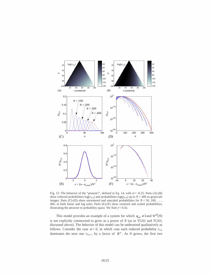
Fig. 15: The behavior of the “present1”, defined in Eq. 14, with α = -0.25. Parts (A)-(B) show reduced probabilities log(rN,n) and probabilities log(pN,n) up to N = 400 as grayscale images. Parts (C)-(D) show uncentered and unscaled probabilities for N = 50, 100, … , 400, in both linear and log units. Parts (E)-(F) show centered and scaled probabilities, illustrating the attractor in probability space. We find γ = 0.42.
This model provides an example of a system for which 1≠entq and Weff(N) is not explicitly constructed to grow as a power of N (as in TGS2 and TGS3, discussed above). The behavior of this model can be understood qualitatively as follows. Consider the case α < 0, in which case each reduced probability rN,k dominates the next one rN,k+1 by a factor of N α . As N grows, the first two

19/25
probabilities pN,0 and pN,1 are increasingly dominant, becoming approximately
1 – ε and ε, with αε +1~ N . Clearly, as N increases, the BGS entropy of this probability set decreases towards zero. A small value qent tends to emphasize the very small probabilities pN,n for 2n ≥ , effectively drawing the calculation away from the zero entropy point, and ensuring the entropy Sq increases linearly.
-5 -4 -3 -2 -1 0 1 2 30
0.2
0.4
0.6
0.8
1
α
Nmax = 100 q
ent
Fig. 16: Numerical results for extensive qent plotted as a function of the parameter α, for the model “present2” defined in Eq. 16. The symmetry of the model “present1” in α has been broken, and qent = 1 for all 0α ≥ . The solid line is a guide for the eye. The values qent for α < 0 coincide with those of Fig. 14.
The attractor for this model for α = -0.25 is shown in Fig. 15. As α is varied
away from 0 (the independent case), we find the diffusion exponent varies systematically away from the normal case γ = 0.5, and 0γ → as 0α → , as can
be seen in Fig. 20. For |α| > 1, the exponent γ remains 0, indicating a localized state, and consistent with the picture of only two probabilities (PN,0 and pN,1) which are appreciably non-zero.
We now introduce a symmetrized version of this model, referred to as “present2” in Fig. 1B, and defined by
,
n
N n
Nr
Z
α ′
= (16)
where
/ 2
0, ,n n N
n n NN n otherwise
≤⎧ ⎢ ⎥⎣ ⎦′ = =⎨ −⎩… (17)
and where Z is a constant chosen to satisfy normalization. With this definition, 0α > ( 0α < ) corresponds to reduced probabilities that reach a minimum
(maximum) at n = N/2. When 0≥α , this model exhibits 1entq = . When 0α < ,

20/25
n (centered)
N
log(rN,n)
(A)20 40 60 80 100
20
40
60
80
100-80
-60
-40
-20
n (centered)
N
log(pN,n)
(B)20 40 60 80 100
20
40
60
80
100
-15
-10
-5
0
-200 -100 0 100 2000
0.02
0.04
0.06
0.08
(n - N/2)
pN
,n
(C)-200 -100 0 100 200
10-50
10-40
10-30
10-20
10-10
100
pN
,n
(n - N/2) (D)
N = 250
N = 100
-2 0 20
0.1
0.2
0.3
0.4
(|N/2 - n| - ncenter)/Nγ
Nγ p
N,n
(E)-10 -5 0 5
10-50
10-40
10-30
10-20
10-10
100
Nγ
p N,n
(|N/2 - n| - ncenter)/Nγ (F)
Fig. 17: The behavior of the “present2”, defined in Eq. 16, with α = -0.25. Parts (A)-(B) show reduced probabilities log(rN,n) and probabilities log(pN,n) up to N = 400 as grayscale images. Parts (C)-(D) show uncentered and unscaled probabilities for N = 50, 100, … , 400, in both linear and log units. Parts (E)-(F) show centered and scaled probabilities, illustrating the attractor in probability space. We find γ = 0.42.

21/25
n (centered)
N
log(rN,n)
(A)20 40 60 80 100
20
40
60
80
100 -120
-100
-80
-60
-40
-20
n (centered)
N
log(pN,n)
(B)20 40 60 80 100
20
40
60
80
100
-50
-40
-30
-20
-10
-200 -100 0 100 2000
0.02
0.04
0.06
0.08
0.1
(n - N/2)
pN
,n
(C)-200 -100 0 100 200
10-150
10-100
10-50
100
pN
,n
(n - N/2) (D)
N = 250
N = 100
-2 0 20
0.05
0.1
0.15
0.2
0.25
(|N/2 - n| - ncenter)/Nγ
Nγ
p N,n
(E)-40 -30 -20 -10 0 10
10-150
10-100
10-50
100
Nγ
p N,n
(|N/2 - n| - ncenter)/Nγ (F)
Fig. 18: The behavior of the “present2”, defined in Eq. 16, with α = -0.5. Parts (A)-(B) show reduced probabilities log(rN,n) and probabilities log(pN,n) up to N = 400 as grayscale images. Parts (C)-(D) show uncentered and unscaled probabilities for N = 50, 100, … , 400, in both linear and log units. Parts (E)-(F) show centered and scaled probabilities, illustrating the attractor in probability space. We find γ = 0.28.
qent behaves quantitatively like the model “present1” defined in Eq. 14 above. However, as α decreases we expect to see a difference, because the smallest pN,n in this model (“present2”) are not as small as the smallest pN,n in the model “present1”. The behavior of qent as a function α is shown in Fig. 16. Due to the symmetry of this model about N/2, the attractor for this model has two branches, as shown for α = -0.25 and α = -0.5 in Figs 17 and 18, respectively, and is scaled with ordinate measured from the point of symmetry.

22/25
-5 -4 -3 -2 -1 0 1 20
0.2
0.4
0.6
0.8
1d = 10
d = 5d = 4d = 3
d = 2
α
q ent
Nmax = 200
Fig. 19: Numerical results for extensive qent plotted as a function of the parameter α, for the model “present3”, defined in Eq. 18. Shown are plots for d = 2, 3, 4, 5, and 10. For
0≥α , we observe qent = 1 – 1/d, as predicted based on reduced occupancy. For α < 0, rapidly decreasing probabilities, coupled with explicitly reduced occupancy, leads to
behavior much like that in the model “present 1”, where 1
~−αq as −∞→α . In the
region -1 < α < 0, we find the two effects in competition, leading to more complex behavior. The inset contains a log-log plot of the negative α portion of the data, showing
explicitly that 1
~−αentq , and the sharp change in behavior at α = -1.
Finally, we introduce a version of this model, referred to as “present3” in
Fig. 1B, with a cutoff, similar to the cutoff introduced in the model TGS2. The model is defined by
,
0 otherwise
n
N n
Nn d
Zr
α⎧≤⎪= ⎨
⎪⎩
(18)
where Z is a quantity (depending on N) chosen to ensure proper normalization. When 0α ≥ , this model behaves like the model TGS1, with 1 1entq d= − . This similarity holds even though the occupation probabilities are markedly different from those of TGS1. We thus find the behavior is dominated by Weff, which scales as Weff ~ Nd. When α < 0, the effective number of states is further restricted due to the sharply decreasing values of rN,n, and qent behaves much like the models “present1” and “present2” above, which, as −∞→α , require
0→entq . These results are shown in Fig. 19.
10-1
100
101
10-1
100
-α
qen
t
23/25
3. Conclusion
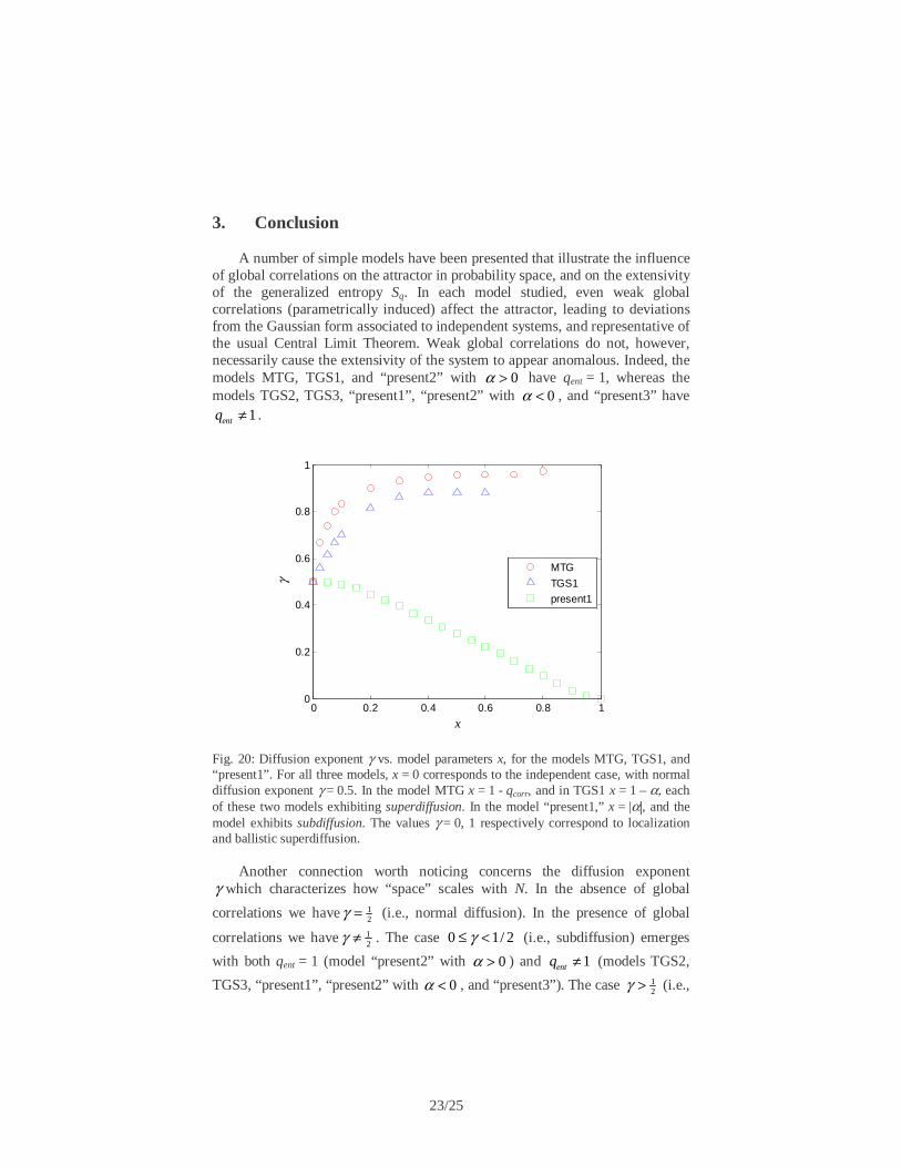
A number of simple models have been presented that illustrate the influence of global correlations on the attractor in probability space, and on the extensivity of the generalized entropy Sq. In each model studied, even weak global correlations (parametrically induced) affect the attractor, leading to deviations from the Gaussian form associated to independent systems, and representative of the usual Central Limit Theorem. Weak global correlations do not, however, necessarily cause the extensivity of the system to appear anomalous. Indeed, the models MTG, TGS1, and “present2” with 0α > have qent = 1, whereas the models TGS2, TGS3, “present1”, “present2” with 0α < , and “present3” have
1entq ≠ .
0 0.2 0.4 0.6 0.8 10
0.2
0.4
0.6
0.8
1
x
γ
MTG
TGS1
present1
Fig. 20: Diffusion exponent γ vs. model parameters x, for the models MTG, TGS1, and “present1”. For all three models, x = 0 corresponds to the independent case, with normal diffusion exponent γ = 0.5. In the model MTG x = 1 - qcorr, and in TGS1 x = 1 – α, each of these two models exhibiting superdiffusion. In the model “present1,” x = |α|, and the model exhibits subdiffusion. The values γ = 0, 1 respectively correspond to localization and ballistic superdiffusion.
Another connection worth noticing concerns the diffusion exponent
γ which characterizes how “space” scales with N. In the absence of global
correlations we have 12γ = (i.e., normal diffusion). In the presence of global
correlations we have 12γ ≠ . The case 0 1/ 2γ≤ < (i.e., subdiffusion) emerges
with both qent = 1 (model “present2” with 0α > ) and 1entq ≠ (models TGS2,
TGS3, “present1”, “present2” with 0α < , and “present3”). The case 12γ > (i.e.,

24/25
superdiffusion) has only emerged for qent = 1 (models MTG, and TGS1). None of the present models has simultaneously exhibited 1
2γ > and 1entq ≠ , but we
see no reason for such a situation to be excluded a priori. For the particular case of subdiffusion, we have obtained 0γ = (i.e., localization) every time that the probabilistic model had, for increasingly large N, probabilities sensibly different from zero only for a finite width in n (hence for the models TGS2, TGS3, “present2” with 0α > , and “present3”). Finally, all the cases for which γ continuously varies with the model parameter characterizing global correlation are indicated in Fig. 20.
The present results can be considered to be a first step in the understanding of the interconnections between (i) the entropic extensivity, (ii) the attractor in the sense of a central limit theorem, (iii) the type of diffusion, and (iv) the distribution which, under appropriate constraints, extremizes the entropic functional. In the absence of global correlations (and assuming that the variances of the distributions that are being composed are finite, which always is the case for binary random variables) we have respectively qent = 1, a Gaussian attractor, normal diffusion, and the maximization of BGSS yields a Gaussian. The challenge at this stage of course is to attain a similar understanding in the presence of global correlations, either (strictly or asymptotically) scale-invariant or not.
Acknowledgements We have benefited from interesting discussions with S. Umarov, R. Hersh,
S. Steinberg, K. Nelson, W. Thistleton, A. Williams and M. Gell-Mann. JM and CT gratefully acknowledge support from A. Williams of the Air Force Research Laboratory, Information Directorate, and SI International, under contract No. FA8756-04-C-0258. LM acknowledges support from PRONEX and CNPq (Brazilian Agencies).
4. References
1 C. Tsallis, J. Stat. Phys. 52, 479 (1988); M. Gell-Mann and C. Tsallis., eds.,
Nonextensive Entropy - Interdisciplinary Applications (Oxford University Press, New York, 2004); J. P. Boon and C. Tsallis, eds., Nonextensive Statistical Mechanics - New Trends, New Perspectives, Europhysics News 36 (6) (2005).
2 F. Baldovin and A. Robledo, Europhys. Lett. 60, 518 (2002); F. Baldovin and A. Robledo, Phys. Rev. E 66, R045104 (2002); F. Baldovin and A. Robledo, Phys. Rev. E 69, 045202(R) (2004); E. Mayoral and A. Robledo, Physica A 340, 219 (2004); A. Robledo, Physica D 193, 153 (2004); A. Robledo, Physica A 342, 104 (2004); A. Robledo, Physica A 344, 631 (2004); A. Robledo, in Nonextensive Entropy - Interdisciplinary Applications, eds. M. Gell-Mann and C. Tsallis (Oxford University Press, New York, 2004); A.

25/25
Robledo, Proceedings of Statphys-Bangalore (2004), Pramana-Journal of Physics 64, 947 (2005); A. Robledo, Europhysics News 36, 214 (2005); E. Mayoral and A. Robledo, Phys. Rev. E 72, 026209 (2005); E. Mayoral and A. Robledo, cond-mat/0501398 (2005); A. Robledo, F. Baldovin and E. Mayoral, in Complexity, Metastability and Nonextensivity, eds. C. Beck, G. Benedek, A. Rapisarda and C. Tsallis (World Scientific, Singapore, 2005), page 43; F. Baldovin and A. Robledo, cond-mat/0504033 (2005); F. Baldovin and A. Robledo, Phys. Rev. E 72, 066213 (2005); A. Robledo, Molecular Physics 103, 3025 (2005); H. Hernandez-Saldana and A. Robledo, Phys. Rev. E (2006), in press [cond-mat/0507624].
3 G. Casati, C. Tsallis and F. Baldovin, Europhys. Lett. 72, 355 (2005). 4 C. Tsallis, M. Gell-Mann and Y. Sato, Proc. Natl. Acad. Sc. USA 102, 15377
(2005). 5 L.G. Moyano, C. Tsallis and M. Gell-Mann, Europhys. Lett. 73, 813 (2006). 6 G. Jona-Lasinio, Nuovo Cimento B 26, 99 (1975); Phys. Rep. 352, 439 (2001)
and references therein; P.A. Mello and B. Shapiro, Phys. Rev. B 37, 5960 (1988); P.A. Mello and S. Tomsovic, Phys. Rev. B 46, 15963 (1992); M. Bologna, C. Tsallis and P. Grigolini, Phys. Rev. E 62, 2213 (2000); C. Tsallis, C. Anteneodo, L. Borland and R. Osorio, Physica A 324, 89 (2003); C. Tsallis, in Anomalous Distributions, Nonlinear Dynamics and Nonextensivity, eds. H.L. Swinney and C. Tsallis, Physica D 193, 3 (2004); C. Tsallis, Milan J. Mathematics 73, 145 (2005); C. Anteneodo, Physica A 358, 289 (2005); F. Baldovin and A. Stella, cond-mat/0510225 (2005); C. Tsallis, in Proc. International Conference on Complexity and Nonextensivity: New Trends in Statistical Mechanics (Yukawa Institute for Theoretical Physics, Kyoto, 14-18 March 2005), Prog. Theor. Phys. Supplement (2006), in press, eds. S. Abe, M. Sakagami and N. Suzuki, [cond-mat/0510125]; D. Sornette, Critical
Phenomena in Natural Sciences (Springer, Berlin, 2001), page 36. 7 H. Suyari and M. Tsukada, IEEE Transactions on Information Theory 51, 753
(2005); H. Suyari, in Complexity, Metastability and Nonextensivity, eds. C. Beck, G. Benedek, A. Rapisarda and C. Tsallis (World Scientific, Singapore, 2005), page 61. H. Suyari, Physica A (2006), in press [cond-mat/0401546].
8 D.J.B. Soares, C. Tsallis, A.M. Mariz and L.R. da Silva, Europhys. Lett. 70, 70 (2005); S. Thurner and C. Tsallis, Europhys Lett 72, 197 (2005); D.R. White, N. Kejzar, C. Tsallis, D. Farmer and S.D. White, Phys. Rev. E 73, 016119 (2006).
9 J.A. Marsh and S. Earl, Phys. Lett. A, 349, 146 (2006). 10 E.P. Borges, Physica A 340, 95 (2004); L. Nivanen, A. Le Mehaute and Q.A.
Wang, Rep Math Phys 52, 437 (2003). 11 G. Polya, Mathematical Discovery, Vol. 1, p 88 (John Wiley, New York,
1962).