individual employment, household employment and risk of

2013 edition

KS-RA-09-001-EN

-C

M e t h o d o l o g i e s a n d W o r k i n g p a p e r s

ISSN 1977-0375

Individual employment, household employment andrisk of poverty in the EU

A decomposition analysis

2013 edition


Individual employment, household employment andrisk of poverty in the EUA decomposition analysis

Europe Direct is a service to help you find answers to your questions about the European Union.

Freephone number (*):

00 800 6 7 8 9 10 11

(*) Certain mobile telephone operators do not allow access to 00 800 numbers or these calls may be billed.

More information on the European Union is available on the Internet (http://europa.eu). Cataloguing data can be found at the end of this publication. Luxembourg: Publications Office of the European Union, 2013 ISBN 978-92-79-29045-9 ISSN 1977-0375 doi:10.2785/41846 Cat. No KS-RA-13-014-EN-N Theme: Populations and social conditions

Collection: Methodologies & Working papers © European Union, 2013 Reproduction is authorised provided the source is acknowledged.

http://europa.eu

3 Individual employment, household employment and risk of poverty in the EU

Eurostat is the Statistical Office of the European Union (EU). Its mission is to be the leading provider of

high quality statistics on Europe. To that end, it gathers and analyses data from the National Statistical

Institutes (NSIs) across Europe and provides comparable and harmonised data for the EU to use in the

definition, implementation and analysis of EU policies. Its statistical products and services are also of

great value to Europe’s business community, professional organisations, academics, librarians, NGOs, the

media and citizens.

In the field of income, poverty, social exclusion and living conditions, the EU Statistics on Income and

Living Conditions (EU-SILC) is the main source for statistical data at European level.

Over the last years, important progress has been achieved in EU-SILC as a result of the coordinated work

of Eurostat and NSIs.

In June 2010, the European Council adopted a social inclusion target as part of the Europe 2020 Strategy:

to lift at least 20 million people in the EU from the risk of poverty and exclusion by 2020. To monitor

progress towards this target, the 'Employment, Social Policy, Health and Consumer Affairs' (EPSCO) EU

Council of Ministers agreed on an 'at risk of poverty or social exclusion' indicator. To reflect the

multidimensional nature of poverty and social exclusion, this indicator consists of three sub-indicators: i)

at-risk-of-poverty (i.e. low income); ii) severe material deprivation; and iii) living in very low work

intensity households.

In this context, the Second Network for the Analysis of EU-SILC (Net-SILC2) is bringing together

National Statistical Institutes (NSIs) and academic expertise at international level in order to carry out in-

depth methodological work and socio-economic analysis, to develop common production tools for the

whole European Statistical System (ESS) as well as to ensure the overall scientific organisation of the

third and fourth EU-SILC conferences. The current working paper is one of the outputs of the work of

Net-SILC2. It was presented at the third EU-SILC conference (Vienna, December 2012), which was

jointly organised by Eurostat and Net-SILC2 and hosted by Statistics Austria.

It should be stressed that this methodological paper does not in any way represent the views of Eurostat,

the European Commission or the European Union. This is independent research which the authors have

contributed in a strictly personal capacity and not as representatives of any Government or official body.

Thus they have been free to express their own views and to take full responsibility both for the judgments

made about past and current policy and for the recommendations for future policy.

This document is part of Eurostat’s Methodologies and working papers collection, which are technical

publications for statistical experts working in a particular field. These publications are downloadable free

of charge in PDF format from the Eurostat website:

http://epp.eurostat.ec.europa.eu/portal/page/portal/income_social_inclusion_living_conditions/publication

s/methodologies_and_working_papers.

Eurostat databases are also available at this address, as are tables with the most frequently used and

requested short- and long-term indicators.

http://epp.eurostat.ec.europa.eu/portal/page/portal/income_social_inclusion_living_conditions/publications/methodologies_and_working_papers

http://epp.eurostat.ec.europa.eu/portal/page/portal/income_social_inclusion_living_conditions/publications/methodologies_and_working_papers


TABLE OF CONTENTS

1. Introduction .......................................................................................................... 9

2. The distribution of jobs over households ............................................................ 11

2.1 Trends in individual and household employment ....................................................... 11

2.2 Concept of polarization .............................................................................................. 13

2.3 Trends in the distribution of individual employment over households ........................ 14

2.4 Has distribution of jobs become more unequal over time? ........................................ 17

3. Household joblessness and low work-intensity .................................................. 21

3.1 Alternative definitions of household employment ....................................................... 21

3.2 The Social Stratification of Individuals in Jobless and Work-poor Households ......... 23

4. Relation between changes in labour markets and poverty risks ......................... 27

4.1 Relationship between poverty and employment rates ............................................... 27

4.2 Integrated decomposition of labour market trends and poverty changes .................. 28

4.3 Decomposition of changes in poverty rates on the basis of household work-

intensity ............................................................................................................................ 33

5. Conclusions ........................................................................................................ 39

6. References ......................................................................................................... 41

7. Appendices ........................................................................................................ 43

7.1 Appendix 1: ‘Conditional’ polarization ........................................................................ 43

7.2 Appendix 2: Convergence in EU? .............................................................................. 47

7.3 Appendix 3: Indicators of work poverty at the household level .................................. 50

7.4 Appendix 4: Probability of joblessness on the individual level ................................... 59


INDIVIDUAL EMPLOYMENT, HOUSEHOLD EMPLOYMENT AND RISK OF POVERTY IN THE EU

A decomposition Analysis

(Vincent CORLUY, Frank VANDENBROUCKE(1))

Abstract: This chapter explores the missing links between employment policy success and

inclusion policy failure. The focus is on individuals in the 20 to 59 age cohort and empirical

analyses are relying on the EU Labour Force Survey (EU LFS) and the EU Survey on Income

and Living Conditions (EU SILC).

The analysis proceeds in two steps. The first step considers the distribution of individual jobs

over households, thus establishing a link between individual employment rates and household

employment rates. Following the work by Gregg, Scutella and Wadsworth (2008, 2010) a

‘polarization index’ is created to measure the size of unequal distribution of employment over

households. Actual changes in household joblessness are decomposed in (i) changes due to

changing individual employment rates and changing household structures and (ii) changes in the

distribution of jobs over households.

The second step in the analysis matches employment at both levels of aggregation with poverty.

Therefore, we decompose changes in the at-risk-of-poverty rates on the basis of (i) changes in

the poverty risks of jobless households, and (ii) changes in the poverty risks of other (non-

jobless) households; (iii) changes in household joblessness due to changes in individual

employment rates and changing household structures and (iv) changes in the distribution of

employment. The proposed technique does yield interesting insights into the trajectories that

individual EU welfare states have followed over the past ten years.

(1) Vincent Corluy is affiliated to the University of Antwerp (Belgium) and Frank Vandenbroucke is affiliated to the University of Leuven and the

University of Antwerp (Belgium). We thank Paul De Beer, Bea Cantillon and colleagues at the Herman Deleeck Centre for Social Policy, Brian Nolan, Anne-Catherine Guio, Tony Atkinson and the participants at a seminar at the KU Leuven and the UvA for precious comments. The usual disclaimers apply. This work has been supported by the second Network for the analysis of EU-SILC (Net-SILC2), funded by Eurostat. The European Commission bears no responsibility for the analyses and conclusions, which are solely those of the authors. Email address for correspondence: [email protected].

mailto:[email protected]

9

1 Introduction

Individual employment, household employment and risk of poverty in the EU

1. Introduction

Is employment the best recipe against poverty of people in working age? At the level of individual

citizens and the households in which they live, participation in the labour market significantly diminishes

the risk of financial poverty. However, what seems evident at the level of individuals and households is

less evident at the country level.

Prior to the financial crisis, the Lisbon Strategy could be regarded as a qualified success in the field of

employment, at least if one assumes there to have been causal relationships between the Lisbon Agenda

and growing employment rates across Europe. On the other hand, though, the Lisbon Strategy largely

failed to deliver on its ambitious promise concerning poverty. Notwithstanding generally higher

employment rates many Member States encountered a standstill in the poverty record. We do not observe

a general conversion of employment policy success in anti-poverty success. Hence, it is important to

understand the missing links between employment policy success (or failure) and inclusion policy success

(or failure). We explore those missing links, relying on the statistical apparatus of the EU Labour Force

Survey (EU LFS) and the EU Survey on Income and Living Conditions (EU SILC).

At the poverty side of the equation, our focus is on the share of individuals at risk of poverty in the 20-to-

59 age cohort. Since the poverty risk of an individual is determined on the basis of the income of the

household to which that individual belongs, the relation between at-risk-of-poverty rates and employment

rates must, first of all, be analyzed at the household level. Hence, we will establish measures of household

employment. Our time frame for the analysis of poverty risks is determined by the use of EU SILC 2005

and EU SILC 2008(1). This short time frame is linked to data limitations, but is also interesting per se, as

we want to study the trajectory of EU welfare states(2) during the ‘good economic years’.

Our inquiry in this chapter is to verify empirically one of the explanations for this disappointing poverty

trends during the ‘good economic years’ of the Lisbon era, put forward in Vandenbroucke and Vleminckx

(2011) and Cantillon (2011), to wit, that this outcome is partly attributable to a failure to reduce the

number of individuals living in jobless or work-poor households, despite increasing individual

employment rates.

The analysis of the poverty trends proceeds in two steps.

The first step considers the distribution of individual jobs over households, thus establishing a link

between individual employment rates and the configuration of household employment. Following the

work by Gregg, Scutella and Wadsworth (2008, 2010), a ‘polarization index’ is defined in terms of the

difference between, on the one hand, the actual share of individuals living in jobless households and, on

the other, the hypothetical share of individuals living in jobless households assuming that individual

employment is distributed randomly across households. This benchmark of ‘random distribution of jobs’

does not carry a normative meaning. The message should be read as follows, in our understanding: to the

extent that positive polarization is avoidable, it signals an avoidable suboptimal situation for a welfare

state. Not only the (skewness of the) relation between individual and household employment is of interest

for our inquiry, but even more important are the changes in its relation. Actual changes in household

joblessness are determined by changing individual employment rates, changing household composition

structures and a (potentially) changing distribution of individual employment rates. We pay additional

attention to the overall evolution in the distribution of jobs over households in EU Member States over a

longer time frame.

The second step in the analysis integrates the two missing links we explore (the link between individual

(1) Since the income data in SILC refer to the year prior to the survey, the basis of our poverty data spans the years 2004 and 2007 (except in

Ireland and the United Kingdom). The ILO-based definition of jobless households refers to realities in 2005 and 2008 observed immediately before the survey, whilst the definition of ‘work-poor’ households (see Section 4) refers to the 12-month period as the income data. To summarize this complex construal we label the time frame as ‘2004/5-2007/8’.

(2) Currently, 31 countries are involved in the EU SILC process. Romania, Bulgaria and Malta were not yet available in the EU SILC 2005 survey and excluded from the trend analysis. The 2008 EU SILC user database offers information on 27 countries. These are all EU European Member States except France and Malta, but including non-EU members Iceland and Norway. However, as France is again included in the UDB of EU SILC 2009, information of this wave is used for estimating changes in France.

10

1 Introduction


employment rates and the configuration of household employment; the link between the configuration of

household employment and poverty) into one single analysis. Therefore we decompose changes in the at-

risk-of-poverty rates on the basis of (i) changes in the poverty risks of jobless households, (ii) changes in

the poverty risks of other (non-jobless) households, (iii) changes in household joblessness due to changes

in individual employment rates and changing household structures and (iv) changes in polarization. In

principle, this method would allow to assess the impact on at-risk-of-poverty rates of changes in

individual employment rates, ceteris paribus, and the impact on at-risk-of poverty rates of changes in

polarization, ceteris paribus. In practice, data limitations make such an integrated analysis hard, and the

conclusions we will draw can only be tentative.

The proposed technique does yield interesting insights into the trajectories that EU welfare states have

followed over the past ten years. The analysis uncovers a puzzling combination of convergence and

disparity within the EU. Polarization levels and household sizes constitute important structural

background features for EU welfare states; together with differences in social spending, they help explain

differences in their performance with regard to poverty risks and poverty risk reduction.

This chapter is organised as follows. In Section 0 we describe the (mathematical) relation between

individual and household employment and explore the distribution of jobs over households over the

timespan 1995-2008. This empirical analysis is based on EU-LFS using an ILO concept of employment.

In Section 0 we will introduce a complementary conception of household employment, we compare those

different dividing lines and assess the social stratification of those individuals living in jobless or work-

poor households, introducing EU SILC estimates. Section 0 integrates the missing links between labour

market trends and at-risk-of-poverty changes. First, we explore whether the upward convergence towards

more unequal distribution of jobs is a determining factor in the analysis of poverty evolutions. Second,

we decompose at-risk-of-poverty rates, looking more in depth at the impact of changes in the

retrospective work-intensity of the household and their poverty risks.

11

2 The distribution of jobs over households


2. The distribution of jobs over households

In this section of the chapter we will use an ILO concept of employment. According to this ILO concept

of employment, an individual is in work if employed for at least one hour in the week before the survey.

The household is jobless if no member in the age bracket 20-59 is in employment, so defined. As a short

cut, we will use ‘jobless household rate’ or ‘household joblessness’ to refer to the share of individuals in

the age bracket 20-59 living in jobless households.(3) In Section 2, we will add a different conception of

household employment rates, distinguishing ‘work-poor’ from ‘work-rich’ households applying a

measurement for work-intensity as defined by Eurostat in the framework of Europe 2020.

2.1 Trends in individual and household employment

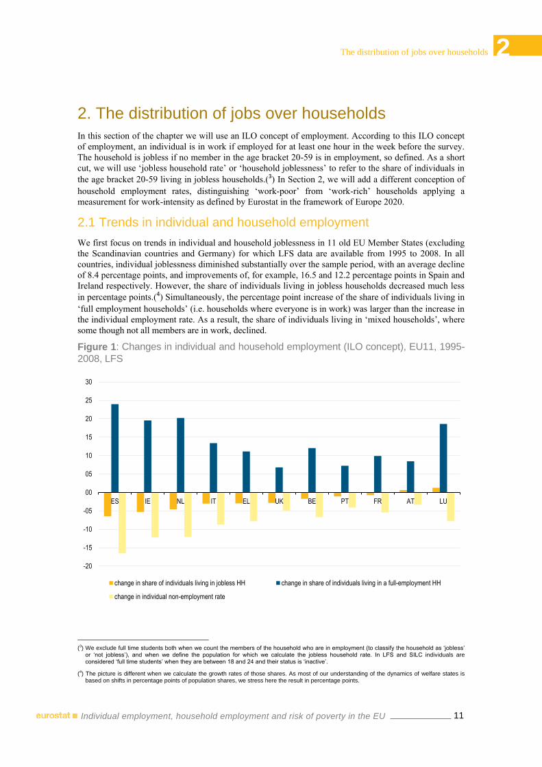
We first focus on trends in individual and household joblessness in 11 old EU Member States (excluding

the Scandinavian countries and Germany) for which LFS data are available from 1995 to 2008. In all

countries, individual joblessness diminished substantially over the sample period, with an average decline

of 8.4 percentage points, and improvements of, for example, 16.5 and 12.2 percentage points in Spain and

Ireland respectively. However, the share of individuals living in jobless households decreased much less

in percentage points.(4) Simultaneously, the percentage point increase of the share of individuals living in

‘full employment households’ (i.e. households where everyone is in work) was larger than the increase in

the individual employment rate. As a result, the share of individuals living in ‘mixed households’, where

some though not all members are in work, declined.

Figure 1: Changes in individual and household employment (ILO concept), EU11, 1995-

2008, LFS

(3) We exclude full time students both when we count the members of the household who are in employment (to classify the household as ‘jobless’

or ‘not jobless’), and when we define the population for which we calculate the jobless household rate. In LFS and SILC individuals are considered ‘full time students’ when they are between 18 and 24 and their status is ‘inactive’.

(4) The picture is different when we calculate the growth rates of those shares. As most of our understanding of the dynamics of welfare states is based on shifts in percentage points of population shares, we stress here the result in percentage points.

-20

-15

-10

-05

00

05

10

15

20

25

30

ES IE NL IT EL UK BE PT FR AT LU

change in share of individuals living in jobless HH change in share of individuals living in a full-employment HH

change in individual non-employment rate

12



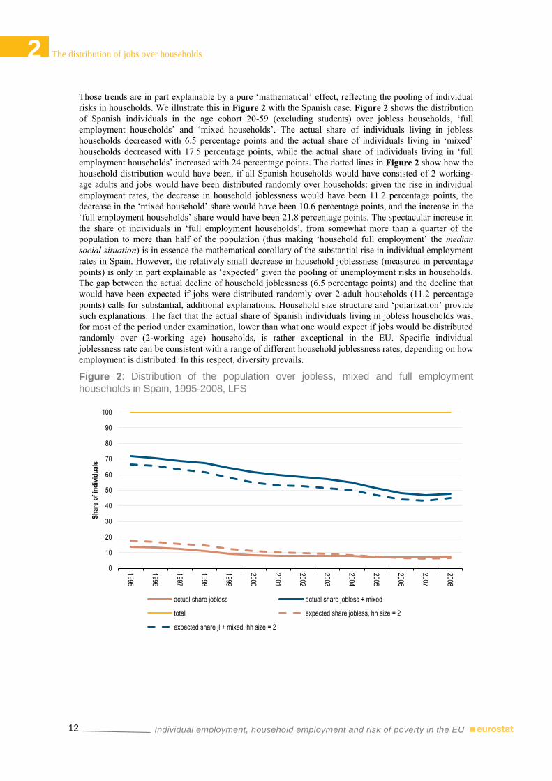
Those trends are in part explainable by a pure ‘mathematical’ effect, reflecting the pooling of individual

risks in households. We illustrate this in Figure 2 with the Spanish case. Figure 2 shows the distribution

of Spanish individuals in the age cohort 20-59 (excluding students) over jobless households, ‘full

employment households’ and ‘mixed households’. The actual share of individuals living in jobless

households decreased with 6.5 percentage points and the actual share of individuals living in ‘mixed’

households decreased with 17.5 percentage points, while the actual share of individuals living in ‘full

employment households’ increased with 24 percentage points. The dotted lines in Figure 2 show how the

household distribution would have been, if all Spanish households would have consisted of 2 working-

age adults and jobs would have been distributed randomly over households: given the rise in individual

employment rates, the decrease in household joblessness would have been 11.2 percentage points, the

decrease in the ‘mixed household’ share would have been 10.6 percentage points, and the increase in the

‘full employment households’ share would have been 21.8 percentage points. The spectacular increase in

the share of individuals in ‘full employment households’, from somewhat more than a quarter of the

population to more than half of the population (thus making ‘household full employment’ the median

social situation) is in essence the mathematical corollary of the substantial rise in individual employment

rates in Spain. However, the relatively small decrease in household joblessness (measured in percentage

points) is only in part explainable as ‘expected’ given the pooling of unemployment risks in households.

The gap between the actual decline of household joblessness (6.5 percentage points) and the decline that

would have been expected if jobs were distributed randomly over 2-adult households (11.2 percentage

points) calls for substantial, additional explanations. Household size structure and ‘polarization’ provide

such explanations. The fact that the actual share of Spanish individuals living in jobless households was,

for most of the period under examination, lower than what one would expect if jobs would be distributed

randomly over (2-working age) households, is rather exceptional in the EU. Specific individual

joblessness rate can be consistent with a range of different household joblessness rates, depending on how

employment is distributed. In this respect, diversity prevails.

Figure 2: Distribution of the population over jobless, mixed and full employment

households in Spain, 1995-2008, LFS

0

10

20

30

40

50

60

70

80

90

1001995

1996

1997

1998

1999

2000

2001

2002

2003

2004

2005

2006

2007

2008S

har

e o

f in

div

idu

als

actual share jobless actual share jobless + mixed

total expected share jobless, hh size = 2

expected share jl + mixed, hh size = 2

13



Although one can observe a rather mathematical relation between individual and household employment,

this does not mean that its relation carries no societal meaning. In a modernizing society, with increasing

individual employment rates, the mitigating impact of risk pooling in households (risk with regard to non-

employment) becomes progressively less important in terms of the (percentage point) reduction of

household joblessness that corresponds (in a ‘probabilistic’, expected sense) to a reduction in individual

joblessness.(5)

2.2 Concept of polarization

The rather crude distinction between jobless households and other households, based on the ILO concept,

allows the construction and decomposition of a polarization index. Later (in section 0), we will integrate

this measure in the decomposition of at-risk-of-poverty rates.

Gregg and Wadsworth (2008) propose a counterfactual to evaluate polarization in the distribution of

household employment. Like the benchmark used in the Lorenz curve, the counterfactual or predicted

household joblessness rate is the one that would occur if jobs were randomly distributed in the

population, given the specific household size structure in the country under examination. Polarization can

be defined as the difference between the actual and the predicted household joblessness rate. So it

measures the extent to which there are more (or fewer) jobless households than predicted in the case of a

random distribution of employment across individuals, given the national household size structure.

Formally,

( )

with:

( )

Obviously, if the share of smaller households increases, a given rate of individual joblessness may be

expected to lead to higher household joblessness, as, all other things being equal, the probability of

having no-one in work is higher in a smaller household than in a larger one. Ceteris paribus the risk of

household joblessness decreases with household size. In what follows, households are distinguished on

the basis of size only. Hence, in this analysis, the ‘predicted rate’ of household joblessness is a function of

(i) the rate of individual joblessness and (ii) the structure of households in terms of size.

We should emphasize that the expression ‘polarization’ does not carry a normative meaning for us, that

is, we do not consider the benchmark used to define the concept – a random distribution of jobs over

households, given the household size structure – as a normative ideal. In a context of limited job

opportunities ‘positive polarization’ might be seen as a kind of ‘Matthew effect’: a concentration of

additional advantage (say, a second job for the partner of someone who is already employed) for those

who already have some advantage (compared with a household where both partners are jobless);

‘negative polarization’ might be appreciated as a form of solidarity, i.e. a fair distribution of scarce

(5) The argument can best be illustrated in the simple hypothesis that the whole population consists of households with only 2 working-age adults.

For a given individual jobless rate n, a random distribution of jobs implies a household jobless rate wp = n2. Hence, the ratio of ‘household joblessness’ on ‘individual joblessness’ wp/n is equal to n, and thus diminishes with increasing individual employment rates. The marginal impact of changes in n on wp also diminishes with increasing employment rates (dwp/dn = 2n). The argument should be interpreted in terms of changes

in percentage points (i.e. percentage points changes in population shares); the elasticity calculated for marginal changes (ndn

wpdwp

/

/) is in this

case always equal to 2. Our reasoning about poverty rates, employment rates, social spending, etc. is typically in terms of changes in percentage points.

14



employment opportunities. However, we do not suggest that either maximally ‘negative polarization’, or

the benchmark of ‘randomly distributed jobs’ serve a normative ideal. The message rather is that ‘positive

polarization’ comes with a social cost: jobless households of working-age people need to be supported by

social transfers. If that cost is to some extent avoidable, the welfare state is in a sense in a suboptimal

equilibrium.

2.3 Trends in the distribution of individual employment over households

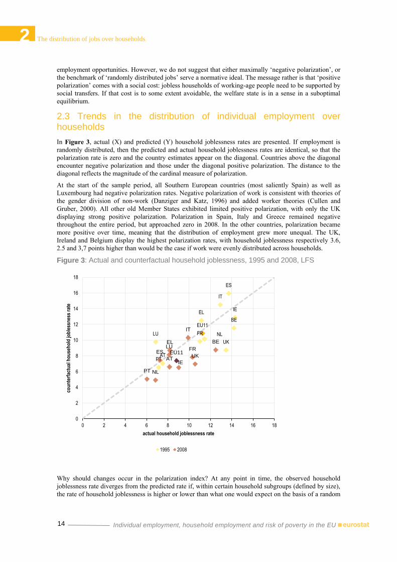
In Figure 3, actual (X) and predicted (Y) household joblessness rates are presented. If employment is

randomly distributed, then the predicted and actual household joblessness rates are identical, so that the

polarization rate is zero and the country estimates appear on the diagonal. Countries above the diagonal

encounter negative polarization and those under the diagonal positive polarization. The distance to the

diagonal reflects the magnitude of the cardinal measure of polarization.

At the start of the sample period, all Southern European countries (most saliently Spain) as well as

Luxembourg had negative polarization rates. Negative polarization of work is consistent with theories of

the gender division of non-work (Danziger and Katz, 1996) and added worker theories (Cullen and

Gruber, 2000). All other old Member States exhibited limited positive polarization, with only the UK

displaying strong positive polarization. Polarization in Spain, Italy and Greece remained negative

throughout the entire period, but approached zero in 2008. In the other countries, polarization became

more positive over time, meaning that the distribution of employment grew more unequal. The UK,

Ireland and Belgium display the highest polarization rates, with household joblessness respectively 3.6,

2.5 and 3,7 points higher than would be the case if work were evenly distributed across households.

Figure 3: Actual and counterfactual household joblessness, 1995 and 2008, LFS

Why should changes occur in the polarization index? At any point in time, the observed household

joblessness rate diverges from the predicted rate if, within certain household subgroups (defined by size),

the rate of household joblessness is higher or lower than what one would expect on the basis of a random

AT

BE

ES

FR

EL IE

IT

LU NL

PT

UK

EU11

AT

BE

ES FR

EL

IE

IT

LU

NL PT

UK EU11

0

2

4

6

8

10

12

14

16

18

0 2 4 6 8 10 12 14 16 18

cou

nte

rfac

tual

ho

use

ho

ld jo

ble

ssn

ess

rate

actual household joblessness rate

1995 2008

15



distribution. Over time, these divergences can decrease or increase in one or more subgroups of the

households; this type of change is referred to as ‘within-household polarization’. There may also be a

structural shift towards household subgroups where polarization is relatively higher, without change in

the subgroup degree of polarization itself; this is referred to as ‘between-household polarization’.

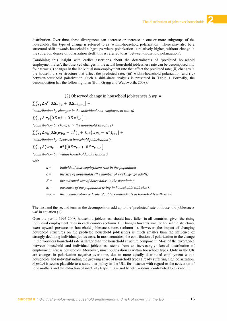
Combining this insight with earlier assertions about the determinants of ‘predicted household

employment rates’, the observed changes in the actual household joblessness rate can be decomposed into

four terms: (i) changes in the individual non-employment rate that affect the predicted rate; (ii) changes in

the household size structure that affect the predicted rate; (iii) within-household polarization and (iv)

between-household polarization. Such a shift-share analysis is presented in Table 1. Formally, the

decomposition has the following form (from Gregg and Wadsworth, 2008):

( )

∑ [ ]

(contribution by changes in the individual non-employment rate n)

∑ [

]

(contribution by changes in the household structure)

∑ ( ) ( ) ]

(contribution by ‘between household polarization’)

∑ ( )[ ]

(contribution by ‘within household polarization’)

with

n = individual non-employment rate in the population

k = the size of households (the number of working-age adults)

K = the maximal size of households in the population

πk = the share of the population living in households with size k

wpk = the actually observed rate of jobless individuals in households with size k

The first and the second term in the decomposition add up to the ‘predicted’ rate of household joblessness

wpe in equation (1).

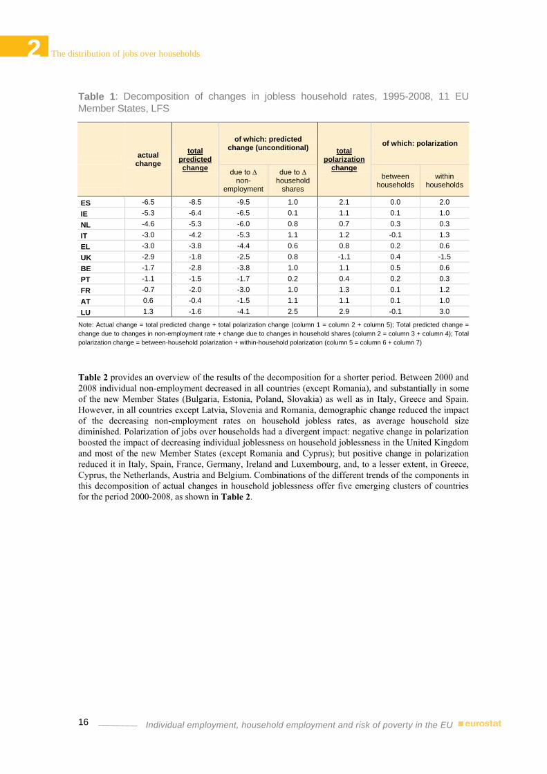
Over the period 1995-2008, household joblessness should have fallen in all countries, given the rising

individual employment rates in each country (column 3). Changes towards smaller household structures

exert upward pressure on household joblessness rates (column 4). However, the impact of changing

household structures on the predicted household joblessness is much smaller than the influence of

strongly declining individual joblessness. In most countries, the contribution of polarization to the change

in the workless household rate is larger than the household structure component. Most of the divergence

between household and individual joblessness stems from an increasingly skewed distribution of

employment across households. Moreover, most polarization is within household types. Only in the UK

are changes in polarization negative over time, due to more equally distributed employment within

households and notwithstanding the growing share of household types already suffering high polarization.

A priori it seems plausible to assume that policy in the UK, for instance with regard to the activation of

lone mothers and the reduction of inactivity traps in tax- and benefit systems, contributed to this result.

16



Table 1: Decomposition of changes in jobless household rates, 1995-2008, 11 EU

Member States, LFS

actual

change

total predicted change

of which: predicted change (unconditional) total

polarization change

of which: polarization

due to ∆ non-

employment

due to ∆ household

shares

between households

within households

ES -6.5 -8.5 -9.5 1.0 2.1 0.0 2.0

IE -5.3 -6.4 -6.5 0.1 1.1 0.1 1.0

NL -4.6 -5.3 -6.0 0.8 0.7 0.3 0.3

IT -3.0 -4.2 -5.3 1.1 1.2 -0.1 1.3

EL -3.0 -3.8 -4.4 0.6 0.8 0.2 0.6

UK -2.9 -1.8 -2.5 0.8 -1.1 0.4 -1.5

BE -1.7 -2.8 -3.8 1.0 1.1 0.5 0.6

PT -1.1 -1.5 -1.7 0.2 0.4 0.2 0.3

FR -0.7 -2.0 -3.0 1.0 1.3 0.1 1.2

AT 0.6 -0.4 -1.5 1.1 1.1 0.1 1.0

LU 1.3 -1.6 -4.1 2.5 2.9 -0.1 3.0

Note: Actual change = total predicted change + total polarization change (column 1 = column 2 + column 5); Total predicted change =

change due to changes in non-employment rate + change due to changes in household shares (column 2 = column 3 + column 4); Total

polarization change = between-household polarization + within-household polarization (column 5 = column 6 + column 7)

Table 2 provides an overview of the results of the decomposition for a shorter period. Between 2000 and

2008 individual non-employment decreased in all countries (except Romania), and substantially in some

of the new Member States (Bulgaria, Estonia, Poland, Slovakia) as well as in Italy, Greece and Spain.

However, in all countries except Latvia, Slovenia and Romania, demographic change reduced the impact

of the decreasing non-employment rates on household jobless rates, as average household size

diminished. Polarization of jobs over households had a divergent impact: negative change in polarization

boosted the impact of decreasing individual joblessness on household joblessness in the United Kingdom

and most of the new Member States (except Romania and Cyprus); but positive change in polarization

reduced it in Italy, Spain, France, Germany, Ireland and Luxembourg, and, to a lesser extent, in Greece,

Cyprus, the Netherlands, Austria and Belgium. Combinations of the different trends of the components in

this decomposition of actual changes in household joblessness offer five emerging clusters of countries

for the period 2000-2008, as shown in Table 2.

17



Table 2: Decomposition of changes in household joblessness rate, 2000-2008, EU27

(exc. SE, FI, DK, MT), LFS

actual

change

total predicted change

of which: predicted change (unconditional) total

polarization change

of which: polarization

due to ∆ non-

employment

due to ∆ household

shares

between households

within households

BG -6.05 -4.5 -6.48 1.98 -1.55 0.05 -1.6

EE -4.51 -3.62 -4.7 1.09 -0.89 0.24 -1.14

PL -3.56 -3.17 -3.51 0.34 -0.39 0.1 -0.49

SK -2.71 -2.43 -2.8 0.38 -0.29 0.11 -0.39

CZ -1.67 -0.58 -1.57 0.99 -1.09 0.37 -1.46

UK -1.01 -0.66 -0.96 0.31 -0.35 0.19 -0.54

LV -3.82 -2.07 -0.94 -1.12 -1.76 0.01 -1.77

SI -2.5 -1.8 -1.61 -0.19 -0.7 -0.06 -0.64

HU -1.09 -0.55 -0.54 0 -0.54 0.01 -0.56

IT -2.07 -2.93 -3.97 1.04 0.86 -0.25 1.11

EL -2 -2.2 -3.06 0.86 0.2 0.04 0.16

CY -1.5 -2.08 -2.22 0.13 0.58 0.14 0.44

NL -1.39 -1.79 -2.21 0.42 0.4 0.16 0.24

ES -1.04 -2.83 -3.6 0.77 1.79 -0.03 1.82

AT -0.71 -1.06 -1.54 0.48 0.35 0.1 0.25

FR -0.58 -1.37 -2.01 0.64 0.8 0.08 0.72

LT -0.43 -1.57 -3.29 1.73 1.14 0.5 0.64

BE -0.35 -0.71 -1.17 0.45 0.36 0.22 0.14

PT 0.64 0.43 0.19 0.24 0.2 0.11 0.1

RO 1.83 1.46 1.86 -0.4 0.38 0.04 0.34

DE 0.25 -0.46 -1.1 0.63 0.72 0.09 0.63

IE 0.57 -0.8 -0.92 0.12 1.37 0.03 1.34

LU 1.1 -0.55 -1.27 0.72 1.66 -0.13 1.79

2.4 Has distribution of jobs become more unequal over time?

In the 11 countries examined (i.e. the Southern, Anglo-Saxon and Continental members of the EU15,

excluding Germany) one observes an upward convergence of the levels of polarization. The pattern is one

of both beta-convergence, a catch-up process, and sigma-convergence, a reduction in the dispersion of

values. In 1995, the average value of the polarization index was 0.39, with a particularly large positive

value in the UK and negative values in Luxembourg, Spain, Italy and Greece (see Figure 4). By 2008 the

average value of the polarization index increased to 1.42.(6) In the UK, positive polarization diminished,

while in Luxembourg, Spain, Italy and Greece the negative polarization characterizing the beginning of

the period was reduced to close to zero. Belgium is an exception in this respect, moving from a rather

high level of positive polarization in 1995 to an even higher level (the highest of the group) by 2008.(7)

(6) Beta-convergence is identified by a negative correlation of -0.81 between the initial values in 1995 and the changes over the period 1995-2008;

sigma-convergence is identified by the standard deviation decreasing from 2.16 to 1.50.The sigma-convergence is quite sensitive to outliers, unlike the beta-convergence. Omission of the UK reduces the decline of standard deviation from -0.66 to -0.35; it also reduces the negative correlation from -0.81 to -0.66.

(7) Appendix 1 shows that the combined impact of region, origin and education is an important explanatory factor for the level of polarization in

Belgium.

18



Figure 4: Levels of polarization in 1995, 2000 and 2008, old and new EU Member

States, LFS

Note: average polarization level in EU11 (avg EU11) excludes Germany from calculations, because estimation for 1995 is missing.

If one restricts the period under consideration to 2000-2008, the number of countries can be increased to

23 (the EU27 minus Sweden, Finland, Denmark and Malta). Between 2000 and 2008, one again observes

beta and (albeit less robustly) sigma-convergence, both for the group of 23 EU Member States and for the

eleven for which data availability stretches back to 1995.(8) There is no real upward convergence in the

levels of polarization across the 23 EU Members: the average value of the polarization index for the

group under review increased from 1.61 in 2000 (with a standard deviation of 1.75) to 1.75 (with a

standard deviation of 1.25). In the smaller group of 11 countries for which data are available from 1995

onwards, the upward movement is more outspoken: in 2000 the average value of the polarization index

for these Member States was 0.73 (standard deviation 1.88) increasing to 1.42 (standard deviation 1.50)

by 2008. This trend seems to have been driven mainly by the declining size of households and the rising

female participation in labour markets in Spain, Italy, France and Greece. The ten new Member States

under examination were characterized by high levels of polarization in 2000 (with an average polarization

index of 2.72); in this respect their starting position in the beginning of the Lisbon era was very different

from that of Spain, Italy and Greece, which were still characterized by negative polarization in 2000 with

extended families still pooling unemployment risks.

(8) The beta-convergence is more robust than the sigma-convergence when eliminating outliers. The negative correlation between starting values

for P, signalling beta-convergence, is -0.71 for the EU23 and -0.70 for the EU11. In appendix 2 we elaborate on the impact of elimination of outliers on the sustainability of convergence.

-3

-2

-1

0

1

2

3

4

5

P (1995) P (2000) P (2008)

19



The choice of the first year of this shorter period, 2000, is dictated primarily by data availability.

However, it appears that 2000 is a useful cut-off in describing the evolution of polarization for some

countries. For instance, in Spain and Ireland, the increase in polarization accelerated after 2000; in

Belgium, and to a lesser extent France, the year 2000 marked the beginning of a deceleration or even a

standstill in polarization. Hence, if one takes account of the timing, there appears to be no uniform pattern

of evolutions across the EU, apart from the general trend of upward convergence. The difference in pace

at which women entered the labour market offers part of the explanation.

A first approach to gaining an understanding of the underlying societal trends that affect polarization

consists in the construction of ‘conditional counterfactuals’. We construct a variety of counterfactual

household employment rates and allow individual employment rates to vary over gender, age and

educational level of working-age household members. One can then compare the ‘unconditional

polarization’ index (the counterfactual being based on household size only) with various ‘conditional

polarization’ indices (see Gregg et al., 2010). Subsequently one can calculate the share (as a percentage)

of the absolute level and the share of the change (again, as a percentage) of the unconditional polarization

index that is explained by gender, age, education, etc., or by combinations of those factors. Applying this

approach shows that the level of polarization is predominantly explained by gender.(9)

A second approach applies regression techniques. A simple regression for the EU11 over 1995-2008

shows that the changes in the ratio of female and male employment rates have a significant and

substantial impact on changes in the unconditional polarization index, while changes in the structure of

educational attainment of the population seem to have no significant impact.

These findings reflect fundamental societal trends in Europe, some of which follow a clear pattern of

convergence, whereas others – surprisingly – show no prima facie convergence at all. The ratio of female

and male employment rates displays very strong beta and sigma-convergence in the EU11 over these

years. However, there is neither beta-convergence nor sigma-convergence with regard to the proportion

of the population with post-secondary education (ISCED levels 5-6) in the EU11 over this period (the

correlation between starting values and change is actually positive, and the dispersion increases); with

regard to the proportion of the population with lower than secondary education (ISCED levels 0-2), the

correlation between starting values and change is mildly negative, but the dispersion is not reduced.

Other results show that ‘increased homogamy’ (increased matching of couples on the basis of education

attainment of the partners) is not an explanatory factor for increasing polarization since 1995, that is,

there is no increasing gap between the degree of homogamy one sees in reality in couples and the degree

of homogamy one would expect if couples are formed at random.

(

9) The level of polarization is explained by gender for more than 50% in Spain (for every single year in 1995-2008, with a minimum of 73%

explained), in Greece (for every single year in 1995-2008, with a minimum of 109% explained), in Italy (for every single year in 1995-2008, with a minimum of 97%) and in Luxembourg (for most years in 1995-2008). The change in the level of polarization is explained for more than 50% by gender in the following cases: Austria (2000-2008, change explained for 61%), Belgium (1995-2008, 62%; and 2000-2008, 67%), Cyprus (2000-2008, 146%), Spain (1995-2008, 57%; and 2000-2008, 64%), Greece (1995-2008, 128%; and 2000-2008, 223%), Ireland (1995-2008, 82%), Italy (1995-2008, 70%), Luxembourg (1995-2008, 59%), the Netherlands (2000-2008, 104%; and 1995-2008, 106%), and Portugal (2000-2008, 51%).

21

3 Household joblessness and low work-intensity


3. Household joblessness and low work-intensity

3.1 Alternative definitions of household employment

In the previous Section of this chapter, we used an ILO concept of employment. In this Section, we will

introduce a different conception of household employment rates, distinguishing ‘work-poor’ from ‘work-

rich’ households. Applying a measurement for work-intensity as defined by Eurostat in the framework of

Europe 2020, we consider a household to be ‘work-poor’, if it’s work-intensity is less than 50%. We will

refer to the latter concept with the notation wp0.5 and refer to the former concept (joblessness) with the

notation wp0. The population reference group is exactly the same for wp0 and wp0.5: ‘adults’ are defined as

those belonging to the 20-59 age bracket excluding full-time students (that is, household members aged

20-24 with ILO status inactive). Similarly, the employment status is checked of household members aged

20-59, excluding full-time students aged 20-24.(10) The underlying employment concept is radically

different though. According to the ILO concept of employment an individual is in work if employed for

at least one hour in the week before the survey; the household is jobless if no member belonging to the

working-age focus group is in employment, so defined. For the calculation of wp0 use can be made of

LFS and SILC, differences in the LFS and SILC samples alas leading to divergent results.(11) In contrast,

in order to calculate wp0.5, work-intensity is defined as the ratio of the total number of months that

working-age household members (excluding students) worked to the total number of months that could,

in theory, have been worked by them. For persons who reported having worked part-time, an estimate of

the number of months in terms of full-time-equivalent was computed on the basis of the number of

usually worked hours at the time of the interview. The indicator wp0.5 can only be calculated on the basis

of SILC.

A comparison of these different dividing lines is not straightforward: the distinction between wp0 and

wp0.5 is a matter not only of degree (no economic activity whatsoever versus limited economic activity)

but also of the timeframe applied: wp0 is based on the week before the survey, whereas wp0.5 is based on

the year prior to the survey (income reference period). Thus, the households identified as jobless may be

households where the week prior to the survey no-one happened to be in employment, even though

household members experienced irregular spells in and out of the labour market in the months before;

with the work-intensity metric, these households would not be identified as jobless but as work-poor.

Unsurprisingly, the average value of wp0.5 across the countries under review is higher than the average

value of wp0: 9.5% of the population aged 20-59 was living in a jobless household and 15.7% of the

population was living in a work-poor household, i.e. a household with work-intensity of less than 50%.

Rather more surprisingly, the poverty risk of the jobless households (pwp0), while typically higher than

the poverty risk for the work-poor (pwp0.5), is lower in Denmark, Greece, Norway, France and Estonia.

Two factors may explain this. First, the ILO-based measure for wp0 is not comparable to the work-

intensity measure used by Eurostat, hence one should not a priori expect an ILO-based calculation of

pwp0 to be higher than a work-intensity based calculation for pwp0.5. Second, even when using the work-

intensity metric to calculate pwp0 (i.e. looking back twelve months, and taking into account both months

and hours worked – which we did not do here) the relation between work-intensity and financial poverty

risks is non-linear in most countries: households with work-intensity equal to zero experience lower

poverty risks than households with work-intensity close to zero but non-zero (European Commission,

2011, p. 157, Chart 21). Prima facie, this may be due to the fact that the group of zero work-intensity

households includes a substantial number of households living on pensions or pre-pensions, even below

the age of 59; early-exit schemes may yield a better income than the unemployment or social assistance

benefits on offer to those who have irregular spells in and out of the labour market.

As a matter of fact, the selection of the population age cohort that is examined, influences not only the

levels of at-risk-of-poverty rates within the work-poor (or jobless) and the work-rich segment of the

(10) Hence, whether or not a household, comprised of two 22-year-old students and a non-student adult of the same age, is a jobless household

depends on the employment status of the non-student only.

(11) This problem is discussed in Nolan and De Graaf (2011) and in appendix 2 of this paper.

22

3 Household joblessness and low work intensity


population, but also the share of individuals living in work-poor or jobless households, and the level of

polarization. This corroborates the social stratification analysis in Section 0 below, which shows that age

has an important impact on an individual’s risk to live in a jobless household. However, we found that

alternative choices for the age cohort, e.g. the 20-49 age bracket, did not have much impact on the overall

picture of our decomposition results. For that reason, we only present results with regard to the 20-59 age

bracket.(12)

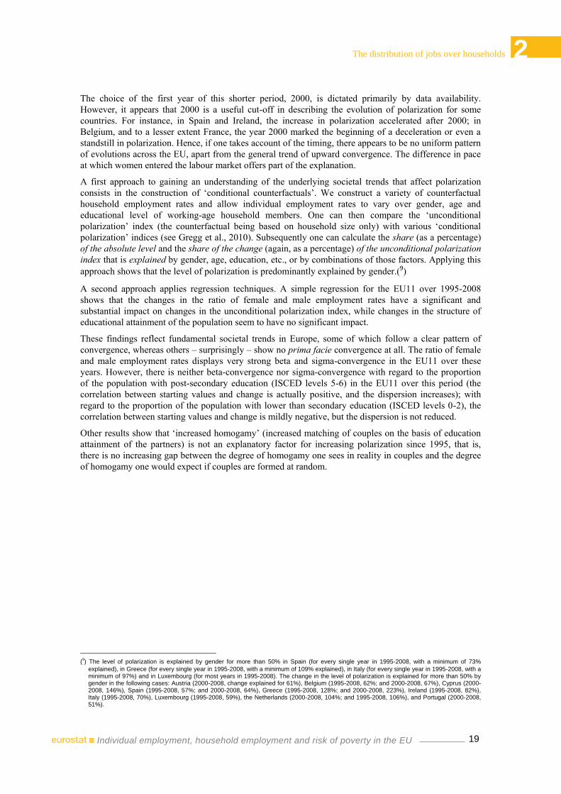
Figure 5: At-risk-of-poverty rate for individuals in jobless and non-jobless households,

2007/8, (ILO definition, EU SILC 2008)

The Europe 2020 strategy focuses on households with ‘very low work-intensity’: very low work-intensity

means a work-intensity of less than 20%. The European Commission shows that the risk of poverty

begins to drop significantly when household work-intensity increases beyond 20%, which explains their

choice of this benchmark. Simultaneously, the Commission shows that the poverty risk (for adults) only

comes down to the same level as the total at-risk-of poverty rate for adults when work-intensity exceeds

50% (European Commission, ibidem). We have chosen to partition the population on the basis of a

benchmark of 50% for several reasons. First, the heterogeneity of the subpopulation with work-intensity

less than 50% does not differ that much from the heterogeneity of the subpopulation with work-intensity

less than 20%. Second, for our purposes the decomposition should focus as much on the work-rich as on

the work-poor segment of the population, and within both groups we want sufficient homogeneity. As a

matter of fact, the changes in at risk of poverty rates are strongly driven by changes related to the work-

rich group. When we expand the work-rich group, by restricting the notion of ‘work-poor’ to ‘very low

work-intensity’ (less than 20%), (a) the position of the work-rich in the decomposition becomes even

more dominant, and (b) their composition becomes more heterogeneous. For these reasons, in Section 0

we pursue a decomposition on the basis of a 50% work-intensity benchmark.

(12) A decomposition of changes in poverty rates (2004/5-2007/8, based on the ILO concept of employment) for the age bracket 20-49 is available

on request.

0

10

20

30

40

50

60

70

80

90

EL DK NL FR NO SE PL AT IS HU SK IT IE FI RO LU BE SI ES PT CZ CY UK LT BG DE EE LV

pwr (wi > 0) pwp (wi = 0)

23



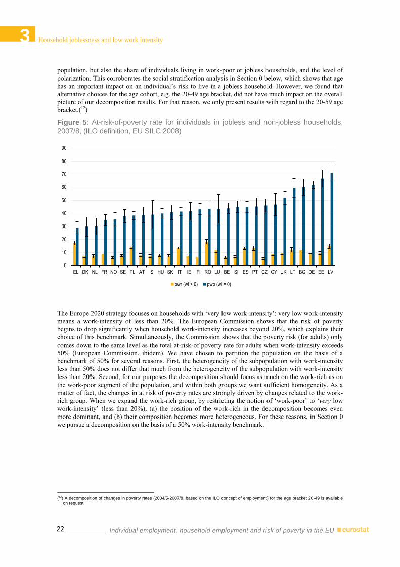
Figure 6: At-risk-of-poverty rate for individuals in work-poor and work-rich households,

2007/8, (EU 2020 definition of work-intensity, EU SILC 2008)

3.2 The Social Stratification of Individuals in Jobless and Work-poor Households

Who are the individuals confronted with a high risk of living in a jobless household (ILO-concept) or a

work-poor household with less than 50% work-intensity (EU2020-concept)? A probit analysis on the

level of EU15 and EU10 reveals strong social stratification, as can be seen in Figure 7 and Figure 8. We

distinguish the old and new Member States, because a priori one might expect a sociological difference

in the stratification of the post-communist societies of the EU10. However, the social stratification of

jobless and work-poor households in today’s ‘old’ and ‘new’ Europe is quite similar; apart from the risk

associated with being single, this social stratification to a large extent reflects some deep-rooted social

disadvantages with which individuals are born or have come to live with rather early in their lives. This

underscores the challenges activation strategies face if they want to reach out successfully at jobless or

work-poor households.

00

10

20

30

40

50

60

70

80

NL IE SE HU AT EL NO PL FR LU SK DK BE CY SI IS IT RO PT CZ ES FI DE UK BG LT EE LV

pwr (wi >= 0.5) pwp (wi < 0.5)

24

3 Household joblessness and low work intensity


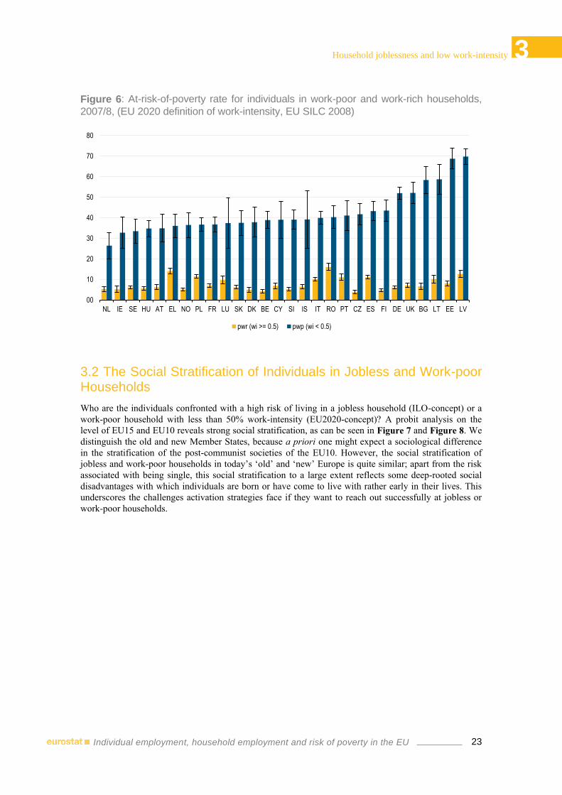
Figure 7: Marginal effects on the probability of living in jobless (ILO) or work-poor (wi <

0.5) households, SILC 2008, for EU15.

First of all and unsurprisingly, individuals with high risks of living in a jobless household or a work-poor

household are individuals living in single households. This result is in part attributable to the mere

‘mathematical’ effect of the absence of unemployment risk pooling in single households. Our probit

analysis does not reveal whether or not singles run a higher risk of joblessness or work poverty as a

‘household’ than their peers in larger households (peers in terms of gender, education, and the other

factors studied in the probit analysis) beyond the higher risk they incur because of the lack of risk

pooling.(13) Rather surprisingly, at the level of these pooled EU data, having children does not influence

the risk of living in a jobless or work-poor household: this is the result of small positive and negative

impact of having children in different Member States, cancelling each other out at the EU15 and EU10

level.(14) Whatever the household size, we see that disabled individuals(15) and individuals whose

educational attainment is lower than secondary education run a higher risk of living in a jobless or work-

poor household. With regard to the risk of living in a jobless household, our age-result follows intuition.

Compared with individuals aged 20-29, individuals between 30-54 have a lower risk and individuals

between 55-59 have a significantly higher risk of living in a jobless household. This result for the latter

group is in line with what one would expect given early exit from labour markets. The marginal effects

are very similar for both the fine-grained definition on the basis of work-intensity and the ILO definition.

(13) In appendix 1 of this paper we refine the decomposition of polarization ‘within’ and ‘between’ households on a conditional basis, which can in

principle shed some light on this question.

(14) That does not exclude that the impact of having children might be important when analysing specific subgroups of the population, for instance singles.

(15) The variable captures the person’s own perception of their main activity at present. The respondent indicates to be permanently disabled or/and unfit to work.

-0,30 -0,20 -0,10 0,00 0,10 0,20 0,30 0,40

sex (male)

age (30-54y)

age (55-59y)

marital status (married)

education (medium)

education (tertiary)

origin (non-EU born)

disabled

2 wa in hh

at least 3 wa in hh

at least 1 child in hh

EU15

wp < 0.5 (eu2020) jl = 0 (ilo)

25



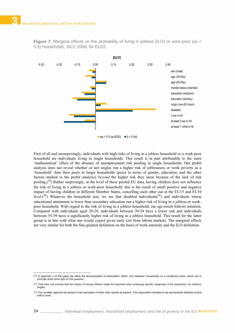
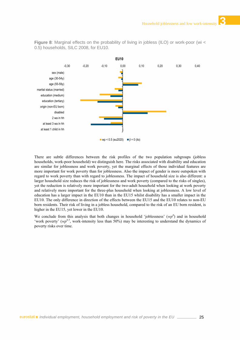
Figure 8: Marginal effects on the probability of living in jobless (ILO) or work-poor (wi <

0.5) households, SILC 2008, for EU10.

There are subtle differences between the risk profiles of the two population subgroups (jobless

households, work-poor household) we distinguish here. The risks associated with disability and education

are similar for joblessness and work poverty, yet the marginal effects of those individual features are

more important for work poverty than for joblessness. Also the impact of gender is more outspoken with

regard to work poverty than with regard to joblessness. The impact of household size is also different: a

larger household size reduces the risk of joblessness and work poverty (compared to the risks of singles),

yet the reduction is relatively more important for the two-adult household when looking at work poverty

and relatively more important for the three-plus household when looking at joblessness. A low level of

education has a larger impact in the EU10 than in the EU15 whilst disability has a smaller impact in the

EU10. The only difference in direction of the effects between the EU15 and the EU10 relates to non-EU

born residents. Their risk of living in a jobless household, compared to the risk of an EU born resident, is

higher in the EU15, yet lower in the EU10.

We conclude from this analysis that both changes in household ‘joblessness’ (wp0) and in household

‘work poverty’ (wp0.5, work-intensity less than 50%) may be interesting to understand the dynamics of

poverty risks over time.

-0,30 -0,20 -0,10 0,00 0,10 0,20 0,30 0,40

sex (male)

age (30-54y)

age (55-59y)

marital status (married)

education (medium)

education (tertiary)

origin (non-EU born)

disabled

2 wa in hh

at least 3 wa in hh

at least 1 child in hh

EU10

wp < 0.5 (eu2020) jl = 0 (ilo)

27

4 Relation between changes in labour markets and poverty risks


4. Relation between changes in labour markets and

poverty risks

4.1 Relationship between poverty and employment rates

On a cross-country level, national rates of household ‘joblessness’ and household ‘work poverty’

calculated on the basis of EU SILC correlate in a different way with national poverty risks for individuals

in the age cohort 20 to 59.

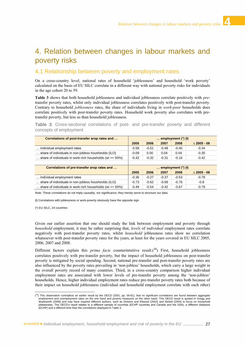
Table 3 shows that both household joblessness and individual joblessness correlate positively with pre-

transfer poverty rates, whilst only individual joblessness correlates positively with post-transfer poverty.

Contrary to household joblessness rates, the share of individuals living in work-poor households does

correlate positively with post-transfer poverty rates. Household work poverty also correlates with pre-

transfer poverty, but less so than household joblessness.

Table 3: Cross-sectional correlations of post- and pre-transfer poverty and different

concepts of employment

Correlations of post-transfer arop rates and … … employment (*) (ⱡ)

2005 2006 2007 2008 ∆ 2005 - 08

… individual employment rates -0.58 -0.51 -0.48 -0.40 -0.34

… share of individuals in non-jobless housheolds (ILO) -0.09 0.00 0.04 0.04 -0.35

… share of individuals in work-rich households (wi >= 50%) -0.42 -0.32 -0.31 -0.16 -0.42

Correlations of pre-transfer arop rates and … … employment (*) (ⱡ)

2005 2006 2007 2008 ∆ 2005 - 08

… individual employment rates -0.36 -0.27 -0.37 -0.53 -0.78

… share of individuals in non-jobless housheolds (ILO) -0.73 -0.62 -0.69 -0.76 -0.8

… share of individuals in work-rich households (wi >= 50%) -0.49 -0.54 -0.42 -0.67 -0.79

Note: These correlations do not imply causality, nor significance; they merely serve to structure our data.

(ⱡ) Correlations with joblessness or work-poverty obviously have the opposite sign

(*) EU SILC, 24 countries

Given our earlier assertion that one should study the link between employment and poverty through

household employment, it may be rather surprising that, levels of individual employment rates correlate

negatively with post-transfer poverty rates, whilst household joblessness rates show no correlation

whatsoever with post-transfer poverty rates for the years, at least for the years covered in EU SILC 2005,

2006, 2007 and 2008.

Different factors explain this prima facie counterintuitive result.(16) First, household joblessness

correlates positively with pre-transfer poverty, but the impact of household joblessness on post-transfer

poverty is mitigated by social spending. Second, national pre-transfer and post-transfer poverty rates are

also influenced by the poverty rates prevailing in ‘non-jobless’ households, which carry a large weight in

the overall poverty record of many countries. Third, in a cross-country comparison higher individual

employment rates are associated with lower levels of pre-transfer poverty among the ‘non-jobless’

households. Hence, higher individual employment rates reduce pre-transfer poverty rates both because of

their impact on household joblessness (individual and household employment correlate with each other)

(16) This observation contradicts an earlier result by the OECD (2001, pp. 59-61), that no significant correlations are found between aggregate

employment and unemployment rates on the one hand and poverty measures on the other hand. This OECD result is quoted in Gregg and Wadsworth (2008) and may have inspired different authors, such as Dickens and Ellwood (2002) and Nickell (2004) to focus on household joblessness. The OECD’s result relates to a different sample of countries (ECHP countries and Canada and the USA), a different database (ECHP) and a different time than the correlations displayed in Table 3.

28



and because of their impact on pre-transfer poverty among the ‘non-jobless’ segment. Finally, higher

individual employment rates are associated with higher levels of spending on working-age cash benefits.

Higher levels of spending are associated with a larger extent of poverty reduction through social transfers,

both within the jobless and the non-jobless segment of the population. Together, all these elements

explain why in a cross-country comparison post-transfer poverty correlates with individual joblessness

but not with household joblessness.

With regard to changes in at-risk of poverty rates between EU SILC 2005 and EU SILC 2008, both

individual joblessness, household joblessness and household work poverty correlate positively but weakly

with changes in poverty rates, as can be inferred from Table 3 (a correlation coefficient of 0.34 for

changes in individual joblessness, 0.35 for changes in household joblessness ∆wp0, and 0.42 for changes

in household work poverty ∆wp0.5). The decomposition analysis in Sections 0 and 0 focuses on these

changes over time.

4.2 Integrated decomposition of labour market trends and poverty changes

In the first section (0) we described an ‘upward convergence in polarization’ with regard to the

distribution of jobs over households. This ‘upward convergence’ had a substantial impact on the

evolution of household joblessness, certainly in relative terms. In comparison with the predicted evolution

of household joblessness without any change in polarization, over the years 2000-2008 changes in the

distribution of individual employment may have been an important factor in the UK (where a negative

change in polarization boosted the household employment rate) and in Spain, Italy, France, Belgium and

Luxembourg (where a positive change in polarization reduced the improvement in household

employment). The question now is whether polarization is also an important factor in the analysis of

poverty trends.

We examine this question by decomposing changes in the at-risk-of-poverty rates on the basis of (i)

changes in the poverty risks of jobless households, (ii) changes in the poverty risks of other (non-jobless)

households, (iii) changes in household joblessness due to changes in individual employment rates and

changing household structures and (iv) changes in polarization. Thus, we integrate the two missing links

we explore in this paper (the link between individual employment rates and the configuration of

household employment; the link between the configuration of household employment and poverty) into

one single analysis. In principle, this would allow to assess the impact of changes in individual

employment rates on at-risk-of-poverty rates, ceteris paribus, and the impact on at-risk-of poverty rates

of changes in polarization, ceteris paribus. In practice, data limitations make such an integrated analysis

hard, and the conclusions we will draw can only be tentative.

Formally, this second step in this integration exercise proceeds as follows.

The at-risk-of-poverty rate can be written as a weighted average of the at-risk-of-poverty rate of

individuals in jobless households and the at-risk-of-poverty rate of individuals in the other households.

Figure 5 illustrated that the poverty risk of individuals in jobless households (pwp) is much higher than

the poverty risk in the other households (pwr) in all EU Member States. Labelling these other households

as the ‘work-rich’ (the share of individuals in work-rich households wr = 1 - wp), we can write:

( )

where:

( )

( )

Changes over time can be decomposed as:

( ) ( )

29



where, for a change from t=0 to t=1,

, etcetera.

In this way, the change in the overall poverty risk is decomposed into three subcomponents or

contributory factors:

i. a contribution by the change in the at-risk-of-poverty rate of the work-rich;

ii. a contribution by the change in the at-risk-of-poverty rate of the work-poor;

iii. a contribution by the change in the share of the population living in work-poor households.

de Beer (2007), who applied this technique to long-term evolutions between 1980 and 2000, rightly

stresses that a decomposition as such is not a causal analysis. It simply calculates by how much a

decomposable variable changes if one of the factors informing the decomposition changes, all the other

factors being equal. Such a mechanical approach should be interpreted with due caution: it is an

accounting device, that does not imply causality. Moreover, changes in one subcomponent may be

intrinsically linked to changes in other subcomponents of the decomposition. For instance, reducing the

share of people living in work-poor households may be achieved by means of a deliberate policy of

increasing the poverty risk of people in work-poor households through stricter conditionality and less

generosity in unemployment benefits. Or increasing employment may push up the median income, to the

effect that a decreasing share of work-poor households and higher poverty rates go hand in hand.

Conversely, work-poor households may become work-rich because their members accept jobs that are at

the lower end of the pay scale, thus marginally increasing the average risk of poverty of the work-rich

group. Diverging evolutions in household size structure between the work-poor and the work-rich,

implying changes in the poverty gap between the two categories, may also be at play. These examples do

not invalidate the decomposition as such, but rather illustrate a general caveat concerning its

interpretation.

Using equations (1), (2), (3) and (4), it is possible to integrate the decomposition of changes in household

employment and changes in poverty on the basis of following equation:

( ) ( ) ( )

However, this requires that the data used to decompose changes in individual and household employment

and changes in poverty are consistent. Since we must rely on SILC to establish a link between

employment and income, it is only possible to pursue this integrated decomposition from 2004 onwards.

For some countries, there are considerable differences between individual and household employment

data obtained through LFS and SILC, as discussed in de Graaf-Zijl and Nolan (2011). Hence,

circumspection is called for when connecting the analysis based on SILC 2005-2008 with the

employment analyses for 1995-2008 and 2000-2008 based on LFS, as presented in previous Sections. In

order to allow some comparison on a conceptual level the ILO definition of joblessness is applied, even

though SILC makes it possible to define joblessness on a retrospective basis for the twelve months prior

to the survey.

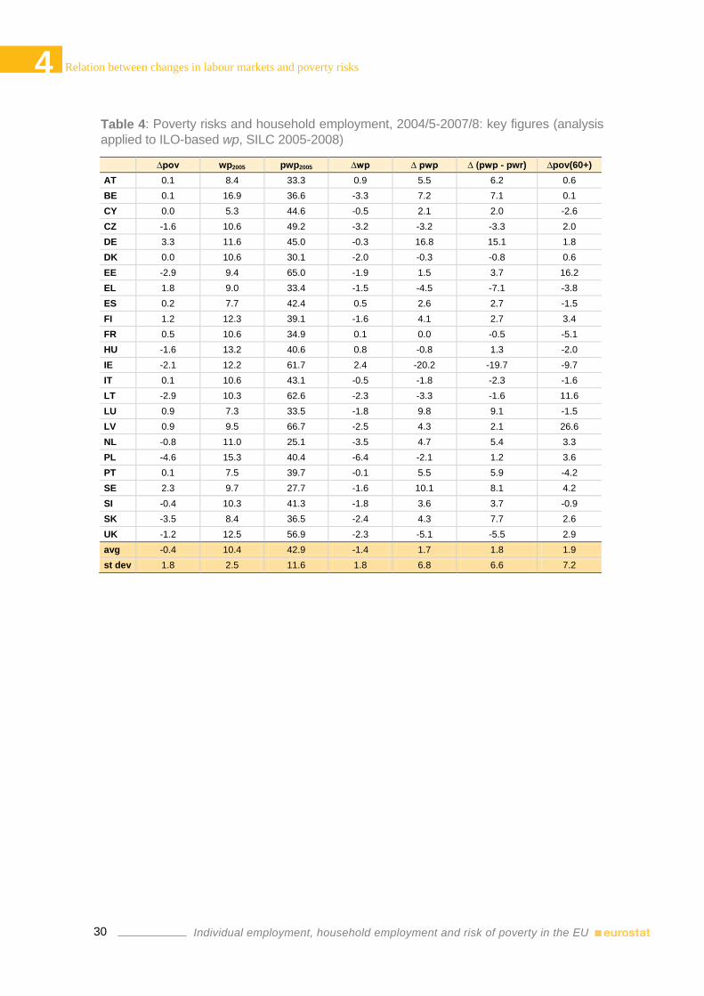
Figure 9 summarizes the integrated decomposition of changes in household joblessness and poverty risks

in the 20-to-59 age bracket on the basis of SILC. The underlying figures are presented in Table 4 and

Table 5 (the statistical significance of the estimated changes in at-risk-of-poverty rates is provided in ).

30



Table 4: Poverty risks and household employment, 2004/5-2007/8: key figures (analysis

applied to ILO-based wp, SILC 2005-2008)

∆pov wp2005 pwp2005 ∆wp ∆ pwp ∆ (pwp - pwr) ∆pov(60+)

AT 0.1 8.4 33.3 0.9 5.5 6.2 0.6

BE 0.1 16.9 36.6 -3.3 7.2 7.1 0.1

CY 0.0 5.3 44.6 -0.5 2.1 2.0 -2.6

CZ -1.6 10.6 49.2 -3.2 -3.2 -3.3 2.0

DE 3.3 11.6 45.0 -0.3 16.8 15.1 1.8

DK 0.0 10.6 30.1 -2.0 -0.3 -0.8 0.6

EE -2.9 9.4 65.0 -1.9 1.5 3.7 16.2

EL 1.8 9.0 33.4 -1.5 -4.5 -7.1 -3.8

ES 0.2 7.7 42.4 0.5 2.6 2.7 -1.5

FI 1.2 12.3 39.1 -1.6 4.1 2.7 3.4

FR 0.5 10.6 34.9 0.1 0.0 -0.5 -5.1

HU -1.6 13.2 40.6 0.8 -0.8 1.3 -2.0

IE -2.1 12.2 61.7 2.4 -20.2 -19.7 -9.7

IT 0.1 10.6 43.1 -0.5 -1.8 -2.3 -1.6

LT -2.9 10.3 62.6 -2.3 -3.3 -1.6 11.6

LU 0.9 7.3 33.5 -1.8 9.8 9.1 -1.5

LV 0.9 9.5 66.7 -2.5 4.3 2.1 26.6

NL -0.8 11.0 25.1 -3.5 4.7 5.4 3.3

PL -4.6 15.3 40.4 -6.4 -2.1 1.2 3.6

PT 0.1 7.5 39.7 -0.1 5.5 5.9 -4.2

SE 2.3 9.7 27.7 -1.6 10.1 8.1 4.2

SI -0.4 10.3 41.3 -1.8 3.6 3.7 -0.9

SK -3.5 8.4 36.5 -2.4 4.3 7.7 2.6

UK -1.2 12.5 56.9 -2.3 -5.1 -5.5 2.9

avg -0.4 10.4 42.9 -1.4 1.7 1.8 1.9

st dev 1.8 2.5 11.6 1.8 6.8 6.6 7.2

31



Figure 9: Decomposition of changes in poverty risks, 2004/5-2007/8; analysis performed

on ILO-based wp, SILC 2005-2008.

Table 5: Decomposition of changes in poverty risks, 2004/5-2007/8; analysis on ILO-

based wp, SILC 2005-2008.

awr.∆pwr awp.∆pwp (apwp - apwr).∆pwe (apwp - apwr).∆P ∆pov

AT -0.67 0.48 0.07 0.17 0.05

BE 0.11 1.1 *** -0.98 *** -0.14 0.09

CY 0.1 0.11 -0.32 0.15 0.04

CZ 0.05 -0.29 -0.67 *** -0.69 -1.6 **

DE 1.49 *** 1.92 *** -0.55 0.41 3.28 ***

DK 0.45 -0.03 -0.31 *** -0.15 -0.03

EE -1.98 *** 0.13 -0.7 *** -0.36 -2.91 ***

EL 2.42 *** -0.37 -0.24 *** 0.02 1.83 **

ES -0.15 0.2 -0.29 0.44 0.2

FI 1.26 *** 0.48 * -0.32 *** -0.25 1.17 ***

FR 0.51 0 0.05 -0.02 0.54

HU -1.75 *** -0.1 -0.18 0.44 -1.59 ***

IE -0.46 -2.7 *** 0.74 *** 0.31 -2.11 ***

IT 0.42 -0.19 -0.2 0.05 0.08

LT -1.51 -0.3 -1.49 *** 0.39 -2.92 ***

LU 0.71 0.63 -0.23 *** -0.26 0.86

LV 1.99 ** 0.35 -1.09 *** -0.3 0.95

NL -0.57 0.44 -0.36 *** -0.35 -0.84

PL -2.86 *** -0.26 -1.27 *** -0.26 -4.64 ***

PT -0.29 0.41 -0.05 0.01 0.08

SE 1.84 *** 0.9 *** -0.48 *** 0.05 2.31 ***

SI -0.08 0.34 -0.61 *** -0.04 -0.39

SK -3.11 *** 0.31 -0.47 *** -0.24 -3.51 ***

UK 0.37 -0.58 ** -0.77 *** -0.26 -1.24 **

Note: ∆pov, ∆pwp and ∆pwr, and (actually observed) ∆wp significantly different from 0 at 95% (***), at 90% (**), at 85% (*).

-6

-5

-4

-3

-2

-1

0

1

2

3

4

5

PL SK LT EE IE CZ HU UK NL SI DK CY AT IT PT BE ES FR LU LV FI EL SE DE

awr . ∆pwr awp . ∆pwp (apwp - apwr) . ∆wpE (apwp - apwr) . ∆P ∆pov "a" = average value

32



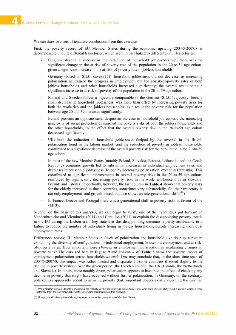
We can draw two sets of tentative conclusions from this exercise.

First, the poverty record of EU Member States during the economic upswing 2004/5-2007/8 is

decomposable in quite different trajectories, which seem in part linked to different policy trajectories:

- Belgium: despite a success in the reduction of household joblessness wp, there was no

significant change in the at-risk-of-poverty rate of the population in the 20-to-59 age cohort,

given a significant increase in the at-risk-of-poverty rate of jobless households.

- Germany (based on SILC, caveat(17)): household joblessness did not decrease, as increasing

polarization neutralised the progress in employment; but the at-risk-of-poverty rates of both

jobless households and other households increased significantly; the overall result being a

significant increase in at-risk-of-poverty of the population in the 20-to-59 age cohort.

- Finland and Sweden follow a trajectory comparable to the German (SILC-)trajectory: here, a

small decrease in household joblessness, was more than offset by increasing poverty risks for

both the work-rich and the jobless households; as a result the poverty risk for the population

between age 20 and 59 increased significantly.

- Ireland presents an opposite case: despite an increase in household joblessness, the increasing

generosity of social protection diminished the poverty risks of both the jobless households and

the other households, to the effect that the overall poverty risk in the 20-to-59 age cohort

decreased significantly.

- UK: both the reduction of household joblessness (helped by the reversal in the British

polarization trend in the labour market) and the reduction of poverty in jobless households,

contributed to a significant decrease of the overall poverty risk for the population in the 20-to-59

age cohort .

- In most of the new Member States (notably Poland, Slovakia, Estonia, Lithuania, and the Czech

Republic) economic growth led to substantial increases in individual employment rates and

decreases in household joblessness (helped by decreasing polarization, except in Lithuania). This

contributed to significant improvements in overall poverty risks in the 20-to-59 age cohort,

reinforced by significantly decreasing poverty risks in the work-rich households in Slovakia,

Poland, and Estonia. Importantly, however, the last column in Table 4 shows that poverty risks

for the elderly increased in those countries, sometimes very substantially. So, their trajectory is

not only employment- and growth-based, but also shows an intergenerational shift.(18)

- In France, Greece and Portugal there was a generational shift in poverty risks in favour of the

elderly.

Second, on the basis of this analysis, we can begin to verify one of the hypotheses put forward in

Vandenbroucke and Vleminckx (2011) and Cantillon (2011) to explain the disappointing poverty trends

in the EU during the Lisbon era. They state that this disappointing outcome is partly attributable to a

failure to reduce the number of individuals living in jobless households, despite increasing individual

employment rates.

Differences among EU Member States in levels of polarization and household size do play a role in

explaining the diversity of configurations of individual employment, household employment and at-risk-

of-poverty rates. How important were changes in employment polarization in explaining changes in

poverty rates? The dark red bars in Figure 9 and column 4 of Table 5 show the poverty impact of

employment polarization across households as such. One may conclude that, in the short time span of

2004/5-2007/8, this impact was rather limited and disparate. In some countries it added slightly to the

decline in poverty realised over the given period (the Czech Republic, the UK, Estonia, the Netherlands

and Slovakia). In others, most notably Spain, polarization appears to have had the effect of checking any

decline in poverty that might have occurred without further polarization. In Germany, on the contrary,

polarization apparently added to growing poverty (but, important doubts exist concerning the German

(17) We entertain serious doubts concerning the validity of the German EU SILC data (Frick and Krell, 2010). They yield a picture which is very

different from the German SOEP data, for crucial components of this analysis.

(18) Hungary and Latvia present diverging trajectories in the group of new Member States.

33



SILC figures).

Obviously, polarization is a long-term trend, rather than a short-term event. Given the fact that the gap

between the poverty risk of jobless households and the poverty risk of non-jobless households is, on

average and across countries, about 33 percentage points, one might say that a one-percentage-point

increase in polarization – which is more or less the average increase for the 11 countries studied between

1995 and 2008 – structurally adds 0.33 percentage points to the proportion of people experiencing

poverty in the 20-to-59 age cohort. This may seem little, but it is certainly not insignificant. However,

polarization does not emerge as ‘structural’, that is, our analysis does not show that it is an unavoidable

process in modernizing societies. Policies do play a role (for evidence on the impact of policies about

patterns of household (non-)participation in labour markets, see for instance Ellwood, 2000; Meyer and

Rosenbaum, 2001; Grogger, 2003).

4.3 Decomposition of changes in poverty rates on the basis of household work-intensity

In Section 0 we pointed out that the correlation between changes in the share of individuals living in

work-poor households and changes in poverty rates is positive, but rather weak (Table 3). This is also

illustrated in Figure 10. This figure is constructed with four quadrants, using changes in poverty (∆pov)

and the share of individuals living in work-poor households (∆wp0.5) between 2005 and 2008 (SILC).

Figure 10: Overall poverty risks and the share of individuals in work-poor household: the

diversity of EU trajectories (EU 2020 definition of work-intensity, EU SILC 2005-2008).

In each of the quadrants one can identify specific trajectories. The Finnish trajectory shows a decreasing

AT BE CY

CZ

DE

DK

EE

ES

FI

FR

EL

HU

IE

IS

IT

LT

LU LV

NL

NO

PL

PT

SE

SI

SK

UK

-6

-4

-2

0

2

4

6

-15 -10 -5 0 5 10 15∆ p

ov

∆ wp

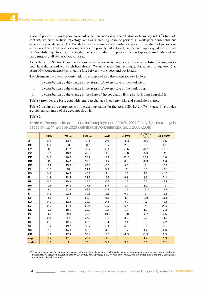
34



share of persons in work-poor households, but an increasing overall at-risk-of-poverty rate.(19) In stark

contrast, we find the Irish trajectory, with an increasing share of persons in work-poor households but

decreasing poverty risks. The Polish trajectory follows a substantial decrease in the share of persons in

work-poor households and a strong decrease in poverty risks. Finally in the right upper quadrant we find

the Swedish trajectory, with a slightly increasing share of persons in work-poor households and an

increasing overall at-risk-of-poverty rate.

As explained in Section 0, we can decompose changes in at-risk-of-poverty rates by distinguishing work-

poor households and work-rich households. We now apply this technique, formalized in equation (4),

using 50% work-intensity as dividing line between work-poor and work-rich.

The change in the overall poverty risk is decomposed into three contributory factors:

i. a contribution by the change in the at-risk-of-poverty rate of the work-rich;

ii. a contribution by the change in the at-risk-of-poverty rate of the work-poor;

iii. a contribution by the change in the share of the population living in work-poor households.

Table 6 provides the basic data with regard to changes in poverty risks and population shares.

Table 7 displays the components of the decomposition for the period 2004/5-2007/8. Figure 11 provides

a graphical summary of the decomposition in

Table 7.

Table 6: Poverty risks and household employment, 2004/5-2007/8: key figures (analysis

based on wp0.5, Europe 2020 definition of work-intensity, SILC 2005-2008)

∆pov Wp2005 pwp2005 ∆wp ∆ pwp ∆ (pwp -

pwr) ∆pov(60+)

AT 0.1 13.2 36.1 2.9 -1.3 -0.5 0.6

BE 0.1 23 36 -2.7 2.9 2.6 0.1

CY 0 11.7 39.7 -0.1 -0.6 -0.7 -2.6

CZ -1.6 13.3 47.5 -1.6 -5.8 -5.6 2

DE 3.3 20.6 38.1 -2.1 13.8 12.1 1.8

DK 0 14.6 37.6 -1.7 0.3 -0.3 0.6

EE -2.9 15.6 65.5 -6.6 3.3 3 16.2

EL 1.8 18 34.1 0.9 2 0.5 -3.8

ES 0.2 16.5 40.8 -2.4 2.5 2.3 -1.5

FI 1.2 18.4 33.7 -4.1 9.8 8.6 3.4

FR 0.5 15.9 35.6 -0.9 1.2 0.5 -5.1

HU -1.6 16.3 37.1 5.9 -2.4 1.1 -2

IE -2.1 21.5 47.8 3.5 -15 -15.3 -9.7

IT 0.1 22.2 39.3 -2.1 0.7 0 -1.6

LT -2.9 17 60.4 -5.6 -1.7 -1.5 11.6

LU 0.9 12.2 32.7 0.8 4.7 4.7 -1.5

LV 0.9 14.8 63.4 -3.7 6.4 4 26.6

NL -0.8 18.1 25.3 -2.5 1.2 1.8 3.3

PL -4.6 29.3 40.5 -10.9 -3.8 -2.7 3.6

PT 0.1 14 37.8 1.1 3.2 3.9 -4.2

SE 2.3 12.5 26.3 1.4 7.1 6 4.2

SI -0.4 19.2 32.7 -5.4 6.3 6.1 -0.9

SK -3.5 14.6 35.8 -4.3 1.7 4.4 2.6

UK -1.2 17.4 53.4 -2.6 -1.3 -1.5 2.9

avg -0.4 17.1 40.7 -1.8 1.5 1.4 1.9

st dev 1.8 4 10.4 3.5 5.5 5.1 7.2

(19) It is tempting to use Germany as an example of a trajectory where the overall poverty rate increases, despite a decreasing share of work-poor

households. As already indicated in footnote 17, doubts exist about EU SILC for Germany. Hence, one should refrain from drawing conclusions on the basis of the former data.

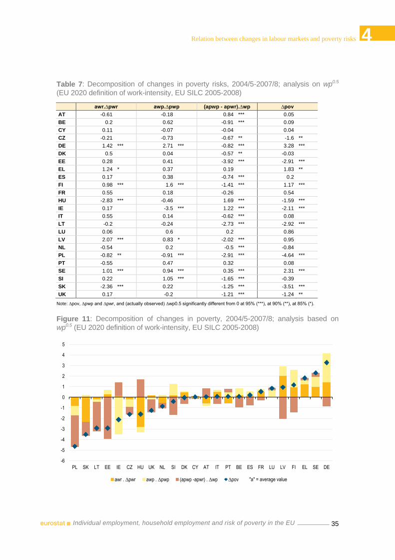
35



Table 7: Decomposition of changes in poverty risks, 2004/5-2007/8; analysis on wp0.5

(EU 2020 definition of work-intensity, EU SILC 2005-2008)

awr.∆pwr awp.∆pwp (apwp - apwr).∆wp ∆pov

AT -0.61 -0.18 0.84 *** 0.05

BE 0.2 0.62 -0.91 *** 0.09

CY 0.11 -0.07 -0.04 0.04

CZ -0.21 -0.73 -0.67 ** -1.6 **

DE 1.42 *** 2.71 *** -0.82 *** 3.28 ***

DK 0.5 0.04 -0.57 ** -0.03

EE 0.28 0.41 -3.92 *** -2.91 ***

EL 1.24 * 0.37 0.19 1.83 **

ES 0.17 0.38 -0.74 *** 0.2

FI 0.98 *** 1.6 *** -1.41 *** 1.17 ***

FR 0.55 0.18 -0.26 0.54

HU -2.83 *** -0.46 1.69 *** -1.59 ***

IE 0.17 -3.5 *** 1.22 *** -2.11 ***

IT 0.55 0.14 -0.62 *** 0.08

LT -0.2 -0.24 -2.73 *** -2.92 ***

LU 0.06 0.6 0.2 0.86

LV 2.07 *** 0.83 * -2.02 *** 0.95

NL -0.54 0.2 -0.5 *** -0.84

PL -0.82 ** -0.91 *** -2.91 *** -4.64 ***

PT -0.55 0.47 0.32 0.08

SE 1.01 *** 0.94 *** 0.35 *** 2.31 ***

SI 0.22 1.05 *** -1.65 *** -0.39

SK -2.36 *** 0.22 -1.25 *** -3.51 ***

UK 0.17 -0.2 -1.21 *** -1.24 **

Note: ∆pov, ∆pwp and ∆pwr, and (actually observed) ∆wp0.5 significantly different from 0 at 95% (***), at 90% (**), at 85% (*).

Figure 11: Decomposition of changes in poverty, 2004/5-2007/8; analysis based on

wp0.5 (EU 2020 definition of work-intensity, EU SILC 2005-2008)

-6

-5

-4

-3

-2

-1

0

1

2

3

4

5

PL SK LT EE IE CZ HU UK NL SI DK CY AT IT PT BE ES FR LU LV FI EL SE DE

awr . ∆pwr awp . ∆pwp (apwp -apwr) . ∆wp ∆pov "a" = average value

36



The percentage point differences between the at-risk-of-poverty rates for respectively work-poor and

work-rich households varies between 20.2 (for the Netherlands) and 59.2 (for Estonia), with an average

of 33.5 percentage points. Correspondingly, the impact of a decrease in the share of individuals living in

work-poor households (wp0.5) by 1 percentage point on the at-risk-of-poverty rate for the whole

population aged 20-59 ranges from -0.2 to -0.6 percentage points, and is, on average, around -0.3

percentage points.(20) Obviously, given the additional diversity of ∆wp0.5 (∆wp0.5 ranges from -10.9 in

Poland to +5.9 in Hungary), the actual contribution to the poverty rate of the change in the share of

people living in work-poor households is very diverse, ranging from -3.9 percentage points in Estonia to

+1.7 percentage points in Hungary (see column 3 in

Table 7).

The observation that the overall cross-sectional correlation between ∆pov and ∆wp0.5 is rather weak

(Table 3) is explained by the highly diversified impact of the other factors at work in the decomposition,

driven by ∆pwp0.5 and ∆pwr0.5. It would be incorrect to assert that the modest decline in the share of

work-poor households was the ‘main culprit’ in explaining disappointing poverty trends across the board

in EU Member States. The picture is both more complicated and more diversified. Moreover, to

contextualize the decomposition of poverty in the 20-59 age bracket, one must also consider the evolution

of poverty in other segments of the population, notably the elderly. For this reason, Table 6 also

incorporates the evolution of the poverty risk of people aged 60+ (hereafter ‘the elderly’).

A first set of observations relates to the overall pattern of change between 2004/5 and 2007/8, a period of

economic growth, particularly in the new Member States. Not surprisingly, with regard to the poverty risk

of both the population aged 20 to 59 and individuals living in work-poor households, one observes

catching-up or beta-convergence (albeit weakened somewhat if one disregards Poland); as regards the

poverty risk of the working-age population, there is also evidence of a sigma-convergence (i.e. less

dispersion, but this effect is weakened quite substantially if Poland is disregarded). However,

simultaneously, the evolution of the gap between the poverty risk of persons in work-poor households

and those in work-rich households is quite diverse: it increased by 12.1 percentage points in Germany, 8.6

percentage points in Finland, 6.1 percentage points in Slovenia, and 6 percentage points in Sweden. In

that same period of just four years, it decreased by 15.3 percentage points in Ireland and 5.6 percentage

points in the Czech Republic. In Germany and Finland, persons in work-poor households lost out in

comparison with, not only the work-rich, but also the elderly. In the Czech Republic and Ireland, persons

in work-poor households gained ground on both the work-rich and the elderly, although the reduction in

poverty risk among the elderly was quite substantial in Ireland. In yet other countries, such as Poland,

Estonia, Lithuania and Latvia, the gap between the work-rich and the work-poor did not change very

much, but the total population aged 20-59 (i.e. both work-poor and work-rich) gained ground on the

elderly, whose poverty risk increased substantially between 2005 and 2008. In other words, Poland,

Estonia, Lithuania and Latvia witnessed an intergenerational shift; the same holds, albeit to a lesser

extent, for the United Kingdom. In France and Greece, too, the gap between the poverty risk of the work-

poor and the work-rich changed hardly at all, though here the elderly gained ground significantly, vis-à-

vis both the work-poor and the work-rich in the population aged 20-59.

We now focus on cases that are in a certain sense exceptional or remarkable. For each of the three

subcomponents in the decomposition, values can be identified in

Table 7 that may be regarded as ‘outliers’ when compared to the average value and standard deviation of

those subcomponents for the twenty-six European countries under review.

Finland is an outlier with regard to the contribution of changes in the poverty risk of work-poor

households, which adds 1.6 percentage points to the overall poverty risk. The decrease in household work

poverty, which was also rather substantial, was not sufficient to offset that impact. Given the fact that the

poverty risk of work-rich households also increased, the overall poverty risk in Finland increased.

The data for Ireland paint exactly the opposite picture. The reduction of poverty among work-poor

households greatly dwarfed the impact of the increasing share of individuals living in work-poor

households over the years 2005-2008. This confirms the intuition on the basis of Figure 10 that, in so far

(20) A regression of ∆pov on ∆wp0.5, ∆pwp0.5 and ∆pwr0.5 yields a coefficient of 0.32 for ∆wp0.5, 0.17 for ∆pwp0.5 and 0.81 for ∆pwr0.5.

37



as the 1990s and the 2000s were concerned, Ireland represented a striking exception.

Poland is exceptional on two counts: the contribution of the declining share of individuals living in work-

poor households (an impact of -2.9 percentage points on the overall poverty rate) and the contribution of

the decreasing poverty risk of work-poor households (an impact of -0.9 percentage points). Together with

a rather large reduction in the poverty risk of the work-rich, this resulted in a substantial overall reduction

in poverty risks. The downside is that the poverty risk of the elderly increased considerably. So one could

say that in Poland the decomposition reveals trends (of pwp0.5 and pwr0.5) that are driven by an

intergenerational shift, i.e. the relative improvement of the position of the cohort aged 20-59 vis-à-vis the

elderly.

Sweden recorded an exceptional increase in poverty over the years considered. This was the result of the

positive impact of all three subcomponents (none were statistical outliers, though all three were rather

high up in the distribution of the value of the subcomponents across the EU). In Sweden, the poverty risk

of the work rich, the work-poor and the elderly increased, and the share of persons in work-poor

households also grew.

Although in Greece the overall poverty risk of the population aged 20-59 increased slightly (though only

significantly at 90%), this was mainly due to the increasing poverty risk of persons in work-rich

households, which was not offset by any other factor at play within that age cohort; the elderly gained the

most ground.

In the United Kingdom, the positive poverty record in the population aged 20-59 (as opposed to the

poverty increase among the elderly) was due mainly to the declining share of people living in work-poor

households. This suggests that activation policies were successful in reaching out to work-poor

households and moving them to the work-rich group.

Although the underlying employment concept is different, we can now compare both poverty risk

decompositions on the basis of wp0.5 and wp0 (Sections 0 and 0). The figures do suggest some interesting

stories. A visual comparison of Figure 9 and Figure 11 shows that the poverty decomposition on the basis

of wp0 is quite different from the decomposition on the basis of wp0.5. The differences are relatively

important for Estonia, Finland, Greece, Hungary, Lithuania, Poland and Slovenia. Some are readily

attributable, as in the case of Poland, where the decomposition on the basis of wp0.5 gives greater weight

to the decline in the share of individuals living in work poverty (as the decrease in wp0.5 is much more

substantial than the decrease in joblessness wp0) and lower weight to the diminishing poverty risk of the

work-rich (since the poverty risk of the work-poor households that hold any job decreases more than the

poverty risk of work-rich households). Despite those differences, the overall picture that emerges with

regard to the diversity of trajectories followed by EU welfare states in the years 2004/5-2007/8 is

confirmed by both decompositions.

39

5 Conclusions


5. Conclusions

The configuration of individual employment rates and household employment rates on which we

focussed in this paper proves relevant for differentiating EU welfare states. We used two concepts to

structure data on household employment: ‘household joblessness’, based on an ILO definition of

employment, and ‘household work poverty’, based on work-intensity. Although the ILO employment

definition is less fine-grained than the work-intensity measure, it has the advantage that it can be

decomposed on the basis of evolutions in individual joblessness, household size structure, and

polarization between and within households.

The shape of this configuration of individual and household employment is driven by forces of

modernization that affect all European welfare states in the same direction, such as declining household size,

feminization of labour markets, … Nevertheless, the configuration is different from country to country.

At the start of the Lisbon era the individual/household employment configuration was rather different in

Spain, Greece and Italy from most other EU Member States, including new Member States. The level of

polarization was negative in Spain, Greece and Italy – a corollary of the pooling of non-employment risks

in extended families – and became gradually less negative. These southern welfare states were in a

trajectory of modernization in which gains in individual employment did not lead to important declines in

the shares of jobless households, i.e. in welfare state dependency. Their welfare states were still in a

process of taking over from familial solidarity.

The pattern in the new Member States after 2000 was very different. Gains in individual employment

rates were enhanced by decreasing polarization of jobs over households, i.e. by a more even distribution

of jobs over households, thus additionally decreasing welfare state dependency. Experience in the UK

suggests that the prevalence of jobless households, and thus the extent of ‘positive’ polarization, can be

influenced by policy.

However, changes in the share of jobless households cannot explain very much of the diversity in the

changes in national at-risk-of-poverty rates during the economic upswing 2004/5-2007/8. Or, to put it in

other ways, it would be incorrect to attribute disappointing poverty trends during the employment boom

years solely to the modest conversion of individual employment successes in household employment

successes, or more specifically to ongoing polarization of jobs over households. But that does not

diminish the importance of national and EU policymakers should attach to the presence of high numbers

of jobless households and polarization, as possibly problematic conditions for welfare states. The

multidimensional Europe 2020 target on social exclusion and poverty, which includes the reduction of

people living in low work-intensity households, may find a justification here.

The disappointing overall ‘stand still’ in national at-risk-of poverty rates during the economic upswing

coincides with a convergence of national at-risk-of-poverty rates in the 20-to-59 age cohort in the EU

during those years. We pursued a decomposition of changes in poverty risks both on the basis of

‘household joblessness’ and ‘household work poverty’. Both suggest that the convergence is the

combined result of four evolutions:

first, an overall poverty standstill in a number of countries, with both relatively low and

relatively high poverty rates;

second, a clearly inegalitarian trajectory in some countries with historically low poverty rates,

such as Sweden and Finland (and Germany, if we base our assessment on EU SILC);

third, a successful effort to reduce poverty in the Anglo-Saxon Member States where poverty

rates were higher, yet with a different policy emphasis in the UK (successful activation) and

Ireland (much enhanced social protection generosity);

fourth, the strong economic and employment growth and an intergenerational shift in poverty

risks in the new Member States.(21

)

(21) There was also an intergenerational shift in some of the old Member States.

40

5 Conclusions


Economic and socio-demographic convergence was a dominant background condition in this short time

span, but the policy trajectories with regard to public social spending on working-age benefits (including

child benefits) were quite different.

These conclusions point simultaneously to the need to refuel economic convergence in the EU, to allow

the new Member States to reconnect on a sound basis with the ‘good years’ in terms of growth and

employment creation, and to the necessary complementarity of employment creation and poverty

reduction through social transfers and inclusive labour market policies.

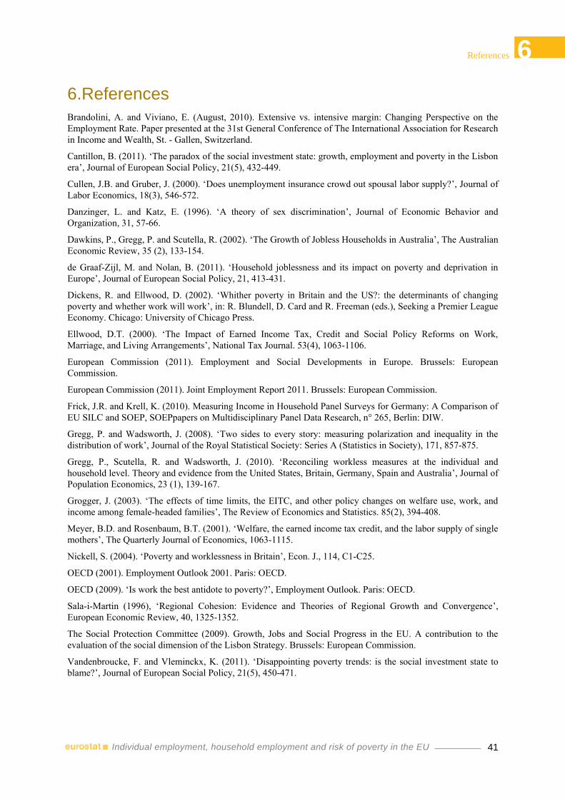
41

6 References


6.References

Brandolini, A. and Viviano, E. (August, 2010). Extensive vs. intensive margin: Changing Perspective on the

Employment Rate. Paper presented at the 31st General Conference of The International Association for Research

in Income and Wealth, St. - Gallen, Switzerland.

Cantillon, B. (2011). ‘The paradox of the social investment state: growth, employment and poverty in the Lisbon

era’, Journal of European Social Policy, 21(5), 432-449.

Cullen, J.B. and Gruber, J. (2000). ‘Does unemployment insurance crowd out spousal labor supply?’, Journal of

Labor Economics, 18(3), 546-572.

Danzinger, L. and Katz, E. (1996). ‘A theory of sex discrimination’, Journal of Economic Behavior and

Organization, 31, 57-66.

Dawkins, P., Gregg, P. and Scutella, R. (2002). ‘The Growth of Jobless Households in Australia’, The Australian

Economic Review, 35 (2), 133-154.

de Graaf-Zijl, M. and Nolan, B. (2011). ‘Household joblessness and its impact on poverty and deprivation in

Europe’, Journal of European Social Policy, 21, 413-431.

Dickens, R. and Ellwood, D. (2002). ‘Whither poverty in Britain and the US?: the determinants of changing

poverty and whether work will work’, in: R. Blundell, D. Card and R. Freeman (eds.), Seeking a Premier League

Economy. Chicago: University of Chicago Press.

Ellwood, D.T. (2000). ‘The Impact of Earned Income Tax, Credit and Social Policy Reforms on Work,

Marriage, and Living Arrangements’, National Tax Journal. 53(4), 1063-1106.

European Commission (2011). Employment and Social Developments in Europe. Brussels: European

Commission.

European Commission (2011). Joint Employment Report 2011. Brussels: European Commission.

Frick, J.R. and Krell, K. (2010). Measuring Income in Household Panel Surveys for Germany: A Comparison of

EU SILC and SOEP, SOEPpapers on Multidisciplinary Panel Data Research, n° 265, Berlin: DIW.

Gregg, P. and Wadsworth, J. (2008). ‘Two sides to every story: measuring polarization and inequality in the

distribution of work’, Journal of the Royal Statistical Society: Series A (Statistics in Society), 171, 857-875.

Gregg, P., Scutella, R. and Wadsworth, J. (2010). ‘Reconciling workless measures at the individual and

household level. Theory and evidence from the United States, Britain, Germany, Spain and Australia’, Journal of

Population Economics, 23 (1), 139-167.

Grogger, J. (2003). ‘The effects of time limits, the EITC, and other policy changes on welfare use, work, and

income among female-headed families’, The Review of Economics and Statistics. 85(2), 394-408.

Meyer, B.D. and Rosenbaum, B.T. (2001). ‘Welfare, the earned income tax credit, and the labor supply of single

mothers’, The Quarterly Journal of Economics, 1063-1115.

Nickell, S. (2004). ‘Poverty and worklessness in Britain’, Econ. J., 114, C1-C25.

OECD (2001). Employment Outlook 2001. Paris: OECD.

OECD (2009). ‘Is work the best antidote to poverty?’, Employment Outlook. Paris: OECD.

Sala-i-Martin (1996), ‘Regional Cohesion: Evidence and Theories of Regional Growth and Convergence’,

European Economic Review, 40, 1325-1352.

The Social Protection Committee (2009). Growth, Jobs and Social Progress in the EU. A contribution to the

evaluation of the social dimension of the Lisbon Strategy. Brussels: European Commission.

Vandenbroucke, F. and Vleminckx, K. (2011). ‘Disappointing poverty trends: is the social investment state to

blame?’, Journal of European Social Policy, 21(5), 450-471.

43

7 Appendices


7. Appendices

7.1 Appendix 1: ‘Conditional’ polarization

The index of polarization measures the deviation of the actual number of jobless households from a random

distribution of employment across all adults aged 20 – 59. The counterfactual household joblessness rate is

determined by individual employment levels and the evolving structure of households. Positive polarization

occurs when there are more jobless households than would be the case with a random distribution of work.

One methodological approach to gain an understanding of the underlying societal conditions in polarization

trends consists in the construction of ‘conditional counterfactuals’ (Dawkins et al., 2002; Gregg et al., 2008), i.e.

a range of counterfactual household employment rates varying by gender, age and educational level of household

members. Relaxing the random distribution of the employment assumption and allowing for varying

employment rates across the key subgroups of the population for which employment is known to vary, make it

possible to explain the concentration of joblessness within certain households. Assortive mating, where members

of the household share common individual characteristics, has an impact on the polarization measure. If

household members have similar characteristics, inequalities in labour market outcomes related to these

characteristics will result in a within-household polarization, especially in the case of randomly distributed

employment across all working age adults. This societal process tends to make joblessness concentrated in

particular households if joblessness occurs more in certain sections of the labour market. The effect of assortive

mating will be stronger if employment opportunities have worsened for certain groups in the population while

having improved for others and the disadvantaged groups live in the same household. For example, demand for

low-educated labour may have fallen simultaneously with an increase in demand for tertiary educated

individuals. When low educated individuals are more likely to live in a household of other low-educated adults

and tertiary educated adults tend to choose for a tertiary educated partner, this can have an effect on employment

polarization.

Subsequently, one can compare the ‘unconditional polarization’ index (the counterfactual being based on

household size only) with several ‘conditional polarization’ indices (see Gregg & Scutella, 2008). The estimation

of this ‘conditional’ counterfactual household joblessness rate allows us to explore whether changes in

employment patterns across age, gender or education (and region or origin) over the last fifteen years lie behind

the observed polarization of work.

We focus on characteristics for which employment rates vary strongly across the population. The characteristics

we use to differentiate between varying employment rates are gender, age (20 – 29 years, 30 – 54 years, 55 – 59

years) and education (at most lower secondary education: ISCED 1-2, upper secondary education: ISCED 3-4,

tertiary education: ISCED 5-6). For Belgium we allow additional variation of individual employment by region

(Flemish, Brussels or Walloon region). We use a combination of these individual characteristics to calculate a

conditional counterfactual household joblessness rate. In Figure A.1 and Figure A.2 we present the actual

household joblessness rate over the period between 1995 and 2009 alongside the counterfactual household

joblessness rate. Initially we assume that employment is distributed randomly. Then we allow employment to

vary across different individual characteristics.

In Spain, the observed share of individuals living in a jobless household is only marginally higher than predicted

by a benchmark of randomly distributed work in 2008. Today then, there is little observed polarization on this

measure. In previous years, the predicted household joblessness rate was higher than the actual share of

household joblessness. This indicates negative polarization. There is negative polarization in countries where

there are fewer jobless households than predicted by a random distribution of individual joblessness. In the

relevant time frame, this occurs mainly in Southern European countries where a more traditional organisation of

the family is still prevalent. One adult works in paid employment while another adult, usually the woman,

remains inactive on the labour market and produces within the home.

44

7 Appendices


In Belgium, the counterfactual household joblessness rate has decreased over time (from 11.6 % in 1995 to 8.8

% in 2008). However, the observed household joblessness rate has broadly remained flat. Therefore polarization

of work across households has increased over time.

Subsequently one can calculate the share (as a percentage) of the absolute level of the unconditional polarization

index that is explained by gender, age, education, etc., or by combinations of those factors. In Figure A.2 and

Figure A.4 we estimate unconditional polarization as the difference between the actual household joblessness

and the unconditional counterfactual household joblessness. The figures show which share of polarization can be

explained when allowing employment to vary across the combined set of characteristics. What remains is called

unexplained (or conditional) polarization.

For Spain, the figures show that allowing employment to vary by gender, age and education decreases the

counterfactual household joblessness rate. This drop is entirely driven by gender related changes. After all,

allowing for gender variations can only fully explain (negative) polarization in Spain. Before 2005, female

employment rates were much lower than those of men. Allowing for gender differences in the counterfactual

employment rate brings on lower predicted household joblessness. Over time the gap in female and male

employment rates has fallen, and by now this effect has entirely disappeared.

For Belgium, variation of individual employment by gender, age and education increases the estimated

counterfactual household joblessness rate, but this effect is very limited. Yet, Figure A.3 shows that the effect of

differences in individual employment rates by region, origin and education is stronger to explain levels of

polarization in Belgium. Because Brussels (and the Walloon region) and non-EU born immigrants are confronted

with low employment rates and adults with those characteristics reside in the same household, individuals living

in those households are likely to have a higher propensity of household joblessness. In combination these

employment changes raise the counterfactual household joblessness by a little more than 1 percentage point, so

even after conditioning around 70 % of the polarization remains (see Figure A.4).

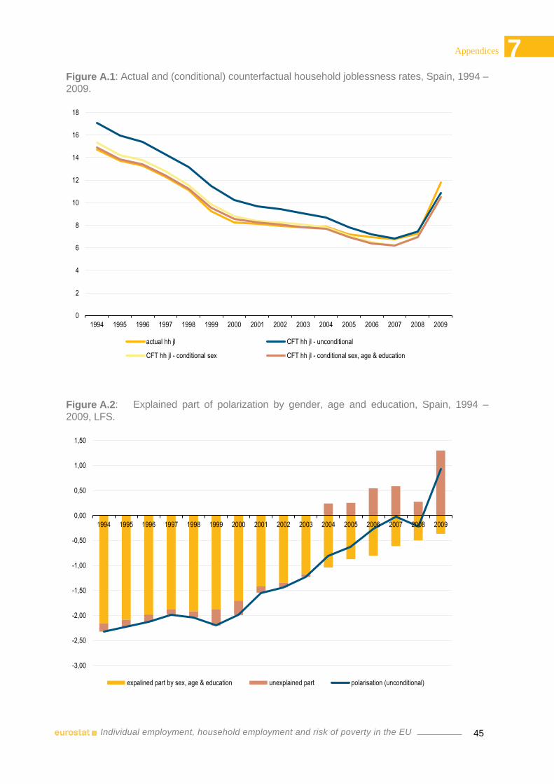
45

7 Appendices


Figure A.1: Actual and (conditional) counterfactual household joblessness rates, Spain, 1994 –

2009.

Figure A.2: Explained part of polarization by gender, age and education, Spain, 1994 –

2009, LFS.

0

2

4

6

8

10

12

14

16

18

1994 1995 1996 1997 1998 1999 2000 2001 2002 2003 2004 2005 2006 2007 2008 2009

actual hh jl CFT hh jl - unconditional

CFT hh jl - conditional sex CFT hh jl - conditional sex, age & education

-3,00

-2,50

-2,00

-1,50

-1,00

-0,50

0,00

0,50

1,00

1,50

1994 1995 1996 1997 1998 1999 2000 2001 2002 2003 2004 2005 2006 2007 2008 2009

expalined part by sex, age & education unexplained part polarisation (unconditional)

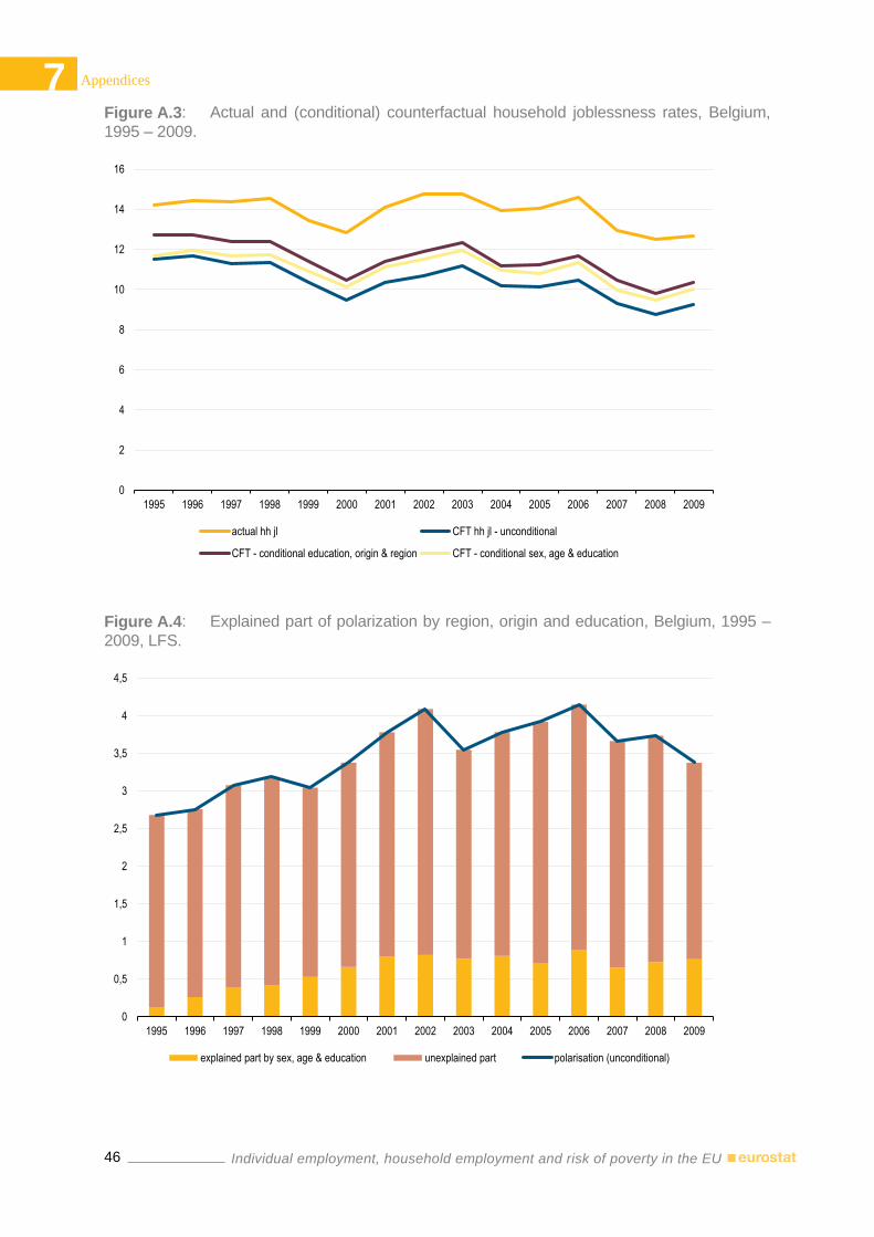
46

7 Appendices


Figure A.3: Actual and (conditional) counterfactual household joblessness rates, Belgium,

1995 – 2009.

Figure A.4: Explained part of polarization by region, origin and education, Belgium, 1995 –

2009, LFS.

0

2

4

6

8

10

12

14

16

1995 1996 1997 1998 1999 2000 2001 2002 2003 2004 2005 2006 2007 2008 2009

actual hh jl CFT hh jl - unconditional

CFT - conditional education, origin & region CFT - conditional sex, age & education

0

0,5

1

1,5

2

2,5

3

3,5

4

4,5

1995 1996 1997 1998 1999 2000 2001 2002 2003 2004 2005 2006 2007 2008 2009

explained part by sex, age & education unexplained part polarisation (unconditional)

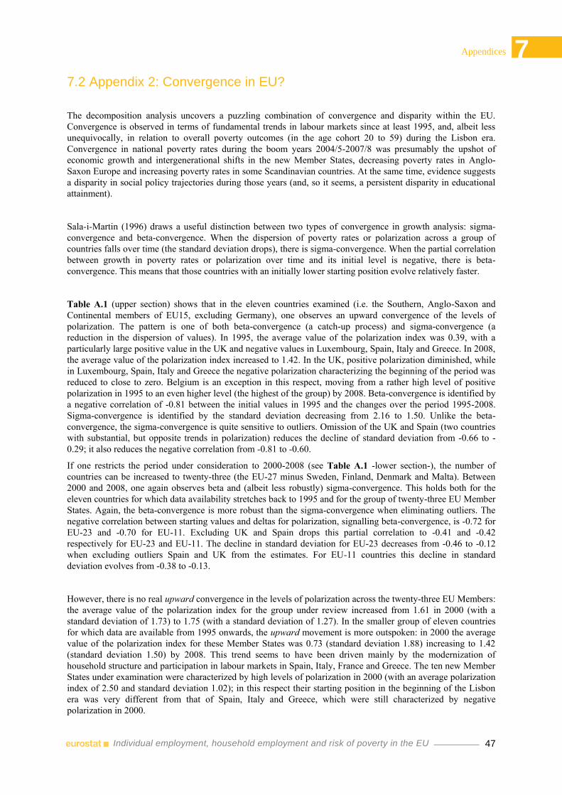
47

7 Appendices


7.2 Appendix 2: Convergence in EU?

The decomposition analysis uncovers a puzzling combination of convergence and disparity within the EU.

Convergence is observed in terms of fundamental trends in labour markets since at least 1995, and, albeit less

unequivocally, in relation to overall poverty outcomes (in the age cohort 20 to 59) during the Lisbon era.

Convergence in national poverty rates during the boom years 2004/5-2007/8 was presumably the upshot of

economic growth and intergenerational shifts in the new Member States, decreasing poverty rates in Anglo-

Saxon Europe and increasing poverty rates in some Scandinavian countries. At the same time, evidence suggests

a disparity in social policy trajectories during those years (and, so it seems, a persistent disparity in educational

attainment).

Sala-i-Martin (1996) draws a useful distinction between two types of convergence in growth analysis: sigma-

convergence and beta-convergence. When the dispersion of poverty rates or polarization across a group of

countries falls over time (the standard deviation drops), there is sigma-convergence. When the partial correlation

between growth in poverty rates or polarization over time and its initial level is negative, there is beta-

convergence. This means that those countries with an initially lower starting position evolve relatively faster.

Table A.1 (upper section) shows that in the eleven countries examined (i.e. the Southern, Anglo-Saxon and

Continental members of EU15, excluding Germany), one observes an upward convergence of the levels of

polarization. The pattern is one of both beta-convergence (a catch-up process) and sigma-convergence (a

reduction in the dispersion of values). In 1995, the average value of the polarization index was 0.39, with a

particularly large positive value in the UK and negative values in Luxembourg, Spain, Italy and Greece. In 2008,

the average value of the polarization index increased to 1.42. In the UK, positive polarization diminished, while

in Luxembourg, Spain, Italy and Greece the negative polarization characterizing the beginning of the period was

reduced to close to zero. Belgium is an exception in this respect, moving from a rather high level of positive

polarization in 1995 to an even higher level (the highest of the group) by 2008. Beta-convergence is identified by

a negative correlation of -0.81 between the initial values in 1995 and the changes over the period 1995-2008.

Sigma-convergence is identified by the standard deviation decreasing from 2.16 to 1.50. Unlike the beta-

convergence, the sigma-convergence is quite sensitive to outliers. Omission of the UK and Spain (two countries

with substantial, but opposite trends in polarization) reduces the decline of standard deviation from -0.66 to -

0.29; it also reduces the negative correlation from -0.81 to -0.60.

If one restricts the period under consideration to 2000-2008 (see Table A.1 -lower section-), the number of

countries can be increased to twenty-three (the EU-27 minus Sweden, Finland, Denmark and Malta). Between

2000 and 2008, one again observes beta and (albeit less robustly) sigma-convergence. This holds both for the

eleven countries for which data availability stretches back to 1995 and for the group of twenty-three EU Member

States. Again, the beta-convergence is more robust than the sigma-convergence when eliminating outliers. The

negative correlation between starting values and deltas for polarization, signalling beta-convergence, is -0.72 for

EU-23 and -0.70 for EU-11. Excluding UK and Spain drops this partial correlation to -0.41 and -0.42

respectively for EU-23 and EU-11. The decline in standard deviation for EU-23 decreases from -0.46 to -0.12

when excluding outliers Spain and UK from the estimates. For EU-11 countries this decline in standard

deviation evolves from -0.38 to -0.13.

However, there is no real upward convergence in the levels of polarization across the twenty-three EU Members:

the average value of the polarization index for the group under review increased from 1.61 in 2000 (with a

standard deviation of 1.73) to 1.75 (with a standard deviation of 1.27). In the smaller group of eleven countries

for which data are available from 1995 onwards, the upward movement is more outspoken: in 2000 the average

value of the polarization index for these Member States was 0.73 (standard deviation 1.88) increasing to 1.42

(standard deviation 1.50) by 2008. This trend seems to have been driven mainly by the modernization of

household structure and participation in labour markets in Spain, Italy, France and Greece. The ten new Member

States under examination were characterized by high levels of polarization in 2000 (with an average polarization

index of 2.50 and standard deviation 1.02); in this respect their starting position in the beginning of the Lisbon

era was very different from that of Spain, Italy and Greece, which were still characterized by negative

polarization in 2000.

48

7 Appendices


With regard to poverty risks, we are restricted to periods of change between 2004/5 and 2007/8, a period of

economic growth, particularly in the new Member States. Not surprisingly, when we look at the poverty risk of

the population aged 20 to 59, we observe catching-up or beta-convergence with a negative correlation of -0.45

between the initial estimates in 2004/5 and the changes over the period 2004/5 and 2007/8 (see Table A.2). This

beta-convergence is weakened if one disregards Poland (negative correlation of -0.33) or if one drops those

countries with the most outspoken trends in poverty risks (i.e. Germany, Ireland, Poland and Sweden) (with a

negative correlation of only -0.18). This beta-convergence also holds for individuals living in work-poor or

jobless households. As regards the poverty risk of the working-age population, there is also evidence of a sigma-

convergence (i.e. less dispersion, but this effect is weakened quite substantially if Poland is disregarded) (see

Table A.3).

Table A.1: BETA & SIGMA-convergence of polarization for different periods (1995 – 2000

– 2008) and different country combinations , SILC.

EU

11 (

=E

U 1

5,

exclu

din

g D

K, F

I, S

E &

DE

)

EU

9 (

=E

U 1

1, e

xclu

din

g U

K &

ES

)

EU

23 (

= E

U27,

exclu

din

g D

K, F

I, S

E &

MT

)

EU

12 (

= E

U15,

exclu

din

g D

K, F

I &

SE

)

EU

11 (

= E

U12 N

MS

, exclu

din

g M

T)

EU

21 (

= E

U23,

exclu

din

g E

S &

UK

)

avg. polarization index 1995 0.39 0.20

2008 1.42 1.36

std. dev. 1995 2.16 1.68

2008 1.5 1.38

sigma convergence '95 - '08 -0.66 -0.29

beta-convergence '95 - '08 -0.81 -0.6

avg. polarization index 2000 0.73 0.67 1.61 0.79 2.5 1.67

2008 1.42 1.36 1.75 1.48 2.03 1.75

std. dev. 2000 1.88 1.52 1.73 1.81 1.02 1.46

2008 1.5 1.38 1.27 1.45 0.88 1.34

sigma convergence '00 - '08 -0.38 -0.13 -0.46 -0.36 -0.13 -0.12

beta-convergence '00 - '08 -0.7 -0.42 -0.72 -0.69 -0.52 -0.41

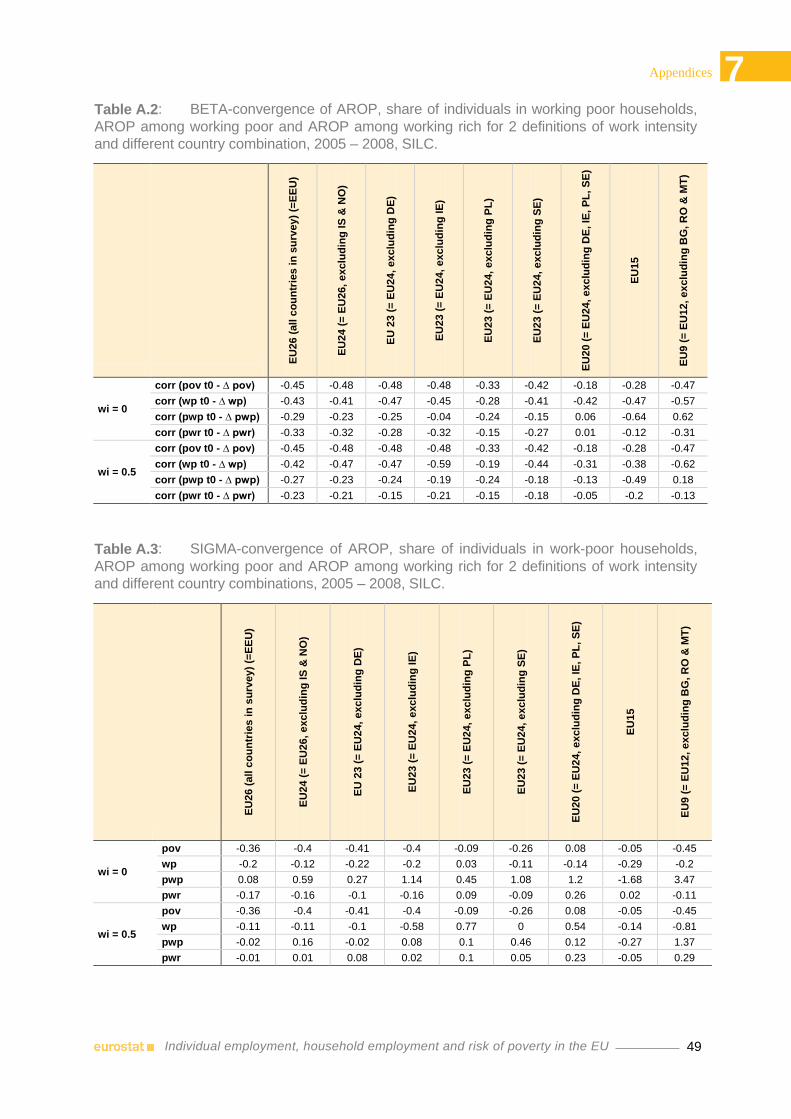
49

7 Appendices


Table A.2: BETA-convergence of AROP, share of individuals in working poor households,

AROP among working poor and AROP among working rich for 2 definitions of work intensity

and different country combination, 2005 – 2008, SILC.

EU

26 (

all c

ou

ntr

ies in

su

rvey)

(=E

EU

)

EU

24 (

= E

U26,

exclu

din

g IS

& N

O)

EU

23 (

= E

U24

, exclu

din

g D

E)

EU

23 (

= E

U24,

exclu

din

g IE

)

EU

23 (

= E

U24,

exclu

din

g P

L)

EU

23 (

= E

U24,

exclu

din

g S

E)

EU

20 (

= E

U24,

exclu

din

g D

E,

IE,

PL

, S

E)

EU

15

EU

9 (

= E

U12,

ex

clu

din

g B

G, R

O &

MT

)

wi = 0

corr (pov t0 - ∆ pov) -0.45 -0.48 -0.48 -0.48 -0.33 -0.42 -0.18 -0.28 -0.47

corr (wp t0 - ∆ wp) -0.43 -0.41 -0.47 -0.45 -0.28 -0.41 -0.42 -0.47 -0.57

corr (pwp t0 - ∆ pwp) -0.29 -0.23 -0.25 -0.04 -0.24 -0.15 0.06 -0.64 0.62

corr (pwr t0 - ∆ pwr) -0.33 -0.32 -0.28 -0.32 -0.15 -0.27 0.01 -0.12 -0.31

wi = 0.5

corr (pov t0 - ∆ pov) -0.45 -0.48 -0.48 -0.48 -0.33 -0.42 -0.18 -0.28 -0.47

corr (wp t0 - ∆ wp) -0.42 -0.47 -0.47 -0.59 -0.19 -0.44 -0.31 -0.38 -0.62

corr (pwp t0 - ∆ pwp) -0.27 -0.23 -0.24 -0.19 -0.24 -0.18 -0.13 -0.49 0.18

corr (pwr t0 - ∆ pwr) -0.23 -0.21 -0.15 -0.21 -0.15 -0.18 -0.05 -0.2 -0.13

Table A.3: SIGMA-convergence of AROP, share of individuals in work-poor households,

AROP among working poor and AROP among working rich for 2 definitions of work intensity

and different country combinations, 2005 – 2008, SILC.

EU

26 (

all c

ou

ntr

ies in

su

rvey)

(=E

EU

)

EU

24 (

= E

U26,

exclu

din

g IS

& N

O)

EU

23 (

= E

U24

, exclu

din

g D

E)

EU

23 (

= E

U24,

exclu

din

g IE

)

EU

23 (

= E

U24,

exclu

din

g P

L)

EU

23 (

= E

U24,

exclu

din

g S

E)

EU

20 (

= E

U24,

exclu

din

g D

E,

IE,

PL

, S

E)

EU

15

EU

9 (

= E

U12,

ex

clu

din

g B

G, R

O &

MT

)

wi = 0

pov -0.36 -0.4 -0.41 -0.4 -0.09 -0.26 0.08 -0.05 -0.45

wp -0.2 -0.12 -0.22 -0.2 0.03 -0.11 -0.14 -0.29 -0.2

pwp 0.08 0.59 0.27 1.14 0.45 1.08 1.2 -1.68 3.47

pwr -0.17 -0.16 -0.1 -0.16 0.09 -0.09 0.26 0.02 -0.11

wi = 0.5

pov -0.36 -0.4 -0.41 -0.4 -0.09 -0.26 0.08 -0.05 -0.45

wp -0.11 -0.11 -0.1 -0.58 0.77 0 0.54 -0.14 -0.81

pwp -0.02 0.16 -0.02 0.08 0.1 0.46 0.12 -0.27 1.37

pwr -0.01 0.01 0.08 0.02 0.1 0.05 0.23 -0.05 0.29

50

7 Appendices


7.3 Appendix 3: Indicators of work poverty at the household level

In this appendix we discuss the existing definitions of household joblessness. We compare the different

demarcations of the relevant populations, the definition of employment and the impact of their combination on

the ranking of countries by their population in household joblessness.

Currently, different indicators for wpα, the share of individuals living in households which we consider ‘work-

poor’ because their work intensity is less than a chosen benchmark value α, are used. In this appendix we list six

indicators, referring to different definitions of household joblessness and/or household work intensity, which one

finds in Eurostat publications and the literature on household employment. Those indicators are based on three

surveys, the EU Labour Force Survey (LFS), the European Community Household Panel (ECHP), and the EU

Survey on Income and Living Conditions (SILC). All these indicators have the same structure. They are

characterized by a population reference group, a working age focus group, and a definition of employment. The

reference group is the population subset which we partition according to the work intensity of households (or, in

the limiting case, the subset which we take into account when calculating the share of individuals in jobless

households and the share not living in jobless households). The working age focus group consists of the

household members on which we focus to determine the work intensity of a household (or, less frequently,

whether or not their household is jobless). In other words, the reference group consists of the potential

“beneficiaries” of economic activity whom we consider relevant for the calculation of the indicator; the focus

group consist of those household members whose potential contribution to economic activity we consider

relevant. The reference group and the focus group may overlap to a large extent, but not necessarily completely.

We examine these indicators in detail in Table A.4 to Table A.7 illustrate that seemingly minor differences in

definitions may translate into differences in analytical and policy emphasis and entail significant changes in

country ranking.

In this paper we have used two indicators for the share of individuals living in work-poor households. Those

measures only differ in the underlying concept of ’employment’: wp0 refers to the share of adults living in

jobless households, using an ILO-concept of employment; wp0.5 refers to the share of adults living in households

that have a work intensity lower than 0.5, using a measurement for work intensity. The population reference

group and the working age focus group are exactly the same. However, in recent scientific literature and policy

debates different definitions of the share of individuals living in work-poor or jobless households have been used

simultaneously. In Table A.4 we compare (a) the population reference group, (b) the working age focus group,

(c) the definition of employment and (d) the data sources of the currently available definitions.

Definition I and definition II are both ‘older’ Eurostat definitions, but are still available online(22). Definition I

determines the share of individuals living in jobless households as (a) the share of individuals aged 18 – 59 who

are living in a household where (b) no adult between 15 and 75 is working. Students aged 18 – 24 who live in

households composed solely of students of the same age group are not included in the calculation. The (c)

employment concept is the ILO definition of employment. Someone is employed when he/she was in paid or

self-employment for at least one hour during the reference week. The household is jobless when no member

belonging to the working age focus group is employed, so defined. Computation of the indicator is based on (d)

LFS.

The indicator in definition II is based on the same employment definition (ILO) and survey data (LFS) as in

definition I, but the population reference group and the working age focus group differ. In definition II the

indicator is calculated as (a) the share of all persons aged 16 – 64 who are living in a household where (b) no-one

between 16 – 64 (excluding dependent children and retired persons) is employed. Additionally, depending on the

number of working age adults in the household, an ordinal measurement of work intensity is introduced.

Definition III is derived from Gregg, Scutella and Wadsworth’s work (2008, 2010) on the relation between

individual and household employment. The indicator is calculated as (a) the share of the total working age

population (20 – 59), excluding full-time students (20 – 24) and all households with a (nominated) head above

retirement age (60 and over), who are living in a household where (b) no-one of this age group is working. The

definition of employment is the ILO concept.

Definition IV captures the ‘new’ household work intensity variable as developed in 2010 in the framework of the

Europe 2020 strategy. For the (d) definition of employment this indicator introduces a work intensity measure of

(22) For definition I see: http://epp.eurostat.ec.europa.eu/tgm/table.do?tab=table&plugin=1&language=en&pcode=tsisc090

For definition II see: http://ec.europa.eu/eurostat/ramon/nomenclatures/index.cfm?TargetUrl=DSP_GLOSSARY_NOM_DTL_VIEW&StrNom=CODED2&StrLanguageCode=EN&IntKey=16624585&RdoSearch=CONTAIN&TxtSearch=work%20intensity&CboTheme=&IntCurrentPage=1

http://epp.eurostat.ec.europa.eu/tgm/table.do?tab=table&plugin=1&language=en&pcode=tsisc090

http://ec.europa.eu/eurostat/ramon/nomenclatures/index.cfm?TargetUrl=DSP_GLOSSARY_NOM_DTL_VIEW&StrNom=CODED2&StrLanguageCode=EN&IntKey=16624585&RdoSearch=CONTAIN&TxtSearch=work%20intensity&CboTheme=&IntCurrentPage=1

http://ec.europa.eu/eurostat/ramon/nomenclatures/index.cfm?TargetUrl=DSP_GLOSSARY_NOM_DTL_VIEW&StrNom=CODED2&StrLanguageCode=EN&IntKey=16624585&RdoSearch=CONTAIN&TxtSearch=work%20intensity&CboTheme=&IntCurrentPage=1

51

7 Appendices


the total work potential during the past year. Work intensity is defined as the ratio of the number of all months

that household members belonging to the working age focus group worked to the total number of months that

could, in theory, have been worked by all the members of the same household who belong to the working age

focus group. For persons who declared having worked part-time, an estimate of the number of months in terms

of the full-time-equivalent is computed on the basis of the number of usually worked hours at the time of the

interview. The indicator is calculated as (a) the share of individuals of 0-59 living in a household where (b) no-

one between 18 – 59 (with the exclusion of students in the age group between 18 and 24) is employed using the

full-time equivalent retrospective definition of employment. In this definition persons are characterized as living

in a household with low work intensity when the household work intensity is below a threshold set at 0.20. The

estimates are based on SILC.

Definition V refers to the (ordinal) measure of work intensity as adopted in 2004 by the Indicators’ Sub-Group

(ISG) of the Social Protection Committee (SPC). It has been used in the breakdown of the social inclusion

secondary indicator ‘at risk of poverty rate by work intensity’. It was calculated (c) as a ratio of the sum of all

months actually worked in the past year (without any distinction between full-time or part-time) by (b) adults

(aged 16-64, excluding dependent inactive youth aged 16-24) to the sum of workable months in the household.

The (a) population reference group is demarcated as the population aged 16-64 excluding dependent inactive

youth aged 16-24. The estimates are based on SILC.

Definition VI uses the same delineations for the working age focus group, the population reference group, the

employment definition and the source data as definition IV, with the sole difference that an ordinal measurement

of work intensity replaces the binary concept of a threshold.

Table A.5 shows the estimates of these different definitions. Looking at individuals living in a jobless household

(work intensity zero), definition VI is clearly the most flexible one. In all countries, the share of individuals

living in a jobless household is the lowest. Comparison of the LFS data estimates learns that definition II is the

most stringent, offering the highest rates of household joblessness. The broader working age focus group

(including individuals aged 60 – 64) can be a relevant explanation. The higher propensity of household

joblessness in definition V as compared to definition VI (both SILC measures) can be explained by the

retrospective question of employment. Not controlling for a full-time equivalent employment of part-time

employees reveals higher rates of household joblessness.

Table A.6 ranks the available countries (dependent of the data source) by the share of individuals living in a

jobless household (work intensity is zero for ordinal measures of work intensity). Minor differences in

definitions translate in significant changes in country rankings.

The discussion of the different definitions of household joblessness shows that available measures do differ in a

number of ways. Besides the data source used, we described differences in population covered, the definition of

employment definitions and the time frame of evaluated work. Given the fact that these indicators differ in all

these respects, it is not surprising that they produce different outcomes. However, to understand the impact of the

data source and to know which of the underlying differences do account for a divergent measurement of the

share of individuals living in household joblessness, we re-calculate definition I in SILC, progressively adapting

the different concepts in the indicator of definition IV (the current EU2020 threshold for individuals living in a

work-poor household). This analysis is shown in Table A.7 (see also table 3 in de Graaf-Zijl and Nolan, 2011) .

Column (1) and column (3) show the point estimates available at the Eurostat website. Column (2) and column

(4) show the same estimates that we have produced ourselves from LFS and SILC data. These estimates are very

similar, indicating that we use the correct definitions and concepts.

In column (5) we retain the concepts of definition IV, but we shift from a work-poor (work intensity < 0.2)

perspective to a joblessness one (work intensity of the household equals zero). For all countries, the share of

individuals living in a jobless household is lower than the share of individuals living in a work-poor household.

The differences, however, are limited indicating that very small jobs are rather exceptional. Bulgaria, Hungary

and Ireland are exceptions with substantial differences between the work-poor and joblessness approach. In

column (6), we alter the population reference group to that of definition I ( from individuals aged 0 - 59 to

individuals aged 18 – 59). The differences between column (5) and (6) are limited. In most countries, excluding

children from the population reference group (hardly) increases the share of individuals living in jobless

households. In Belgium, the Netherland, Denmark and Finland, the increase is more obvious, potentially

indicating that most children do not grow up in joblessness. On the contrary, in the United Kingdom and Ireland

the narrowing of the population reference group to the working age population decreases the share of individuals

living in household joblessness. Subsequently, in column (7) the working age focus group is adapted. Changing

the subset of household members whose potential contribution to economic activity we consider relevant (in this

52

7 Appendices


case from adults aged 18-59y to those aged 15-75y, both excluding students) decreases the share of individuals

living in household joblessness in comparison to column (6). This decline is limited, but most notable in

Southern European countries. Finally, column (7) changes the definition of employment. We switch from a

retrospective work-intensity approach as recently developed in the framework of the new headline targets of the

Europe 2020 strategy to one based on current labour force status during the reference week (ILO). This

adjustment causes the most substantial change in the share of individuals living in jobless households.

Temporary employment, not captured through the ILO definition, is most prominent in the United Kingdom and

Poland, and to a smaller extent in Spain, Finland, Hungary and Ireland. Any remaining differences between

estimates in column (2) and column (8) are solely attributable to reasons related to data sources. For some

countries these differences are quite substantial. We find more than 2 percentage points higher estimates in SILC

in Ireland, Poland and Latvia and we observe 2 per cent point lower estimates in SILC for Luxemburg and

Slovakia. Although both survey samples might have different purposes, with LFS primarily dedicated to the

measurement of employment at the individual level and with SILC mainly constructed for poverty and income

measurement at the household level, these differences are cause for concern for Eurostat and researchers

interested in the relation between individual employment and household poverty.

In Figure A.5 to Figure A.8 we look more closely at the (a) distribution of the population aged 0–59 living in a

jobless household and (b) the distribution of the poor population by work intensity, both defined by the ISG

definition of work intensity (definition V) and the more recent EU2020 definition of work intensity (definition

VI).

The main difference between both definitions is the concept of employment. Although both definitions use a

retrospective approach of employment during the year prior to the survey, definition V controls for the number

of months an individual has been employed while definition VI additionally controls for the number of hours a

part-time employed individual has been working. Thus, in definition V work intensity is defined as the ratio of

the number of all months that household members belonging to the working age focus group worked to the total

number of months that could in theory have been worked by all the members of the same household who belong

to the working age focus group. Additionally, in definition VI, for persons who declared having worked part-

time, an estimate of the number of months in terms of full-time equivalent is computed on the basis of the

number of usually worked hours at the time of the interview.

To improve comparability between both definitions, the population reference group is set at individuals aged 0–

59 years of age for both definitions. The working age focus group is already the same.

Figure A.5 and Figure A.6 show the distribution of the population aged 0–59 by household work intensity in

2009. The following findings arise. First, in all countries, the share of individuals living in a jobless household

(work intensity equals zero) is smaller when one applies definition VI. Controlling for part-time employment

decreases the propensity of living in a jobless household. Second, the share of individuals living in a full

employment household is much more confined when one calculates the estimates with the new EU 2020

definition of work intensity. These differences are most prevalent in the Netherlands and the United Kingdom

with differences of more than 40 percentage points between both definitions of retrospective work intensity. But

also in Austria, Belgium, Germany, Luxembourg and Sweden the differences between both indicators exceed 20

percentage points. Those differences are mainly translated in a trade-off between household full-employment (wi

= 1) and work rich household employment (0.5 <= wi < 1). Thirdly, in the new EU Member States observed

differences in the share of individuals living in full-employment households are rather limited, not exceeding 10

percentage points in any of these countries.

Consequently, the composition of the population at risk of poverty also differs by household work intensity,

depending of the definition applied.

Because of a more rudimentary approach of household work intensity in definition V, the more detailed

subgroups of individuals living in work-poor and work rich households are underrepresented among the poor (at

risk of poverty) population in all countries in comparison with a similar distribution based on definition VI (see

Figure A.7 and Figure A.8). Complementary, the share of individuals living in jobless and full-employment

households are overrepresented among the poor (at risk of poverty) population when one applies definition V to

demarcate work intensity. The overrepresentation of individuals living in jobless households among the poor is

the strongest in Finland, the Netherlands and Poland. The overrepresentation of individuals living in full-

employment households among the poor population is most outspoken in Luxembourg, the Netherlands,

Romania, Sweden and the United Kingdom.

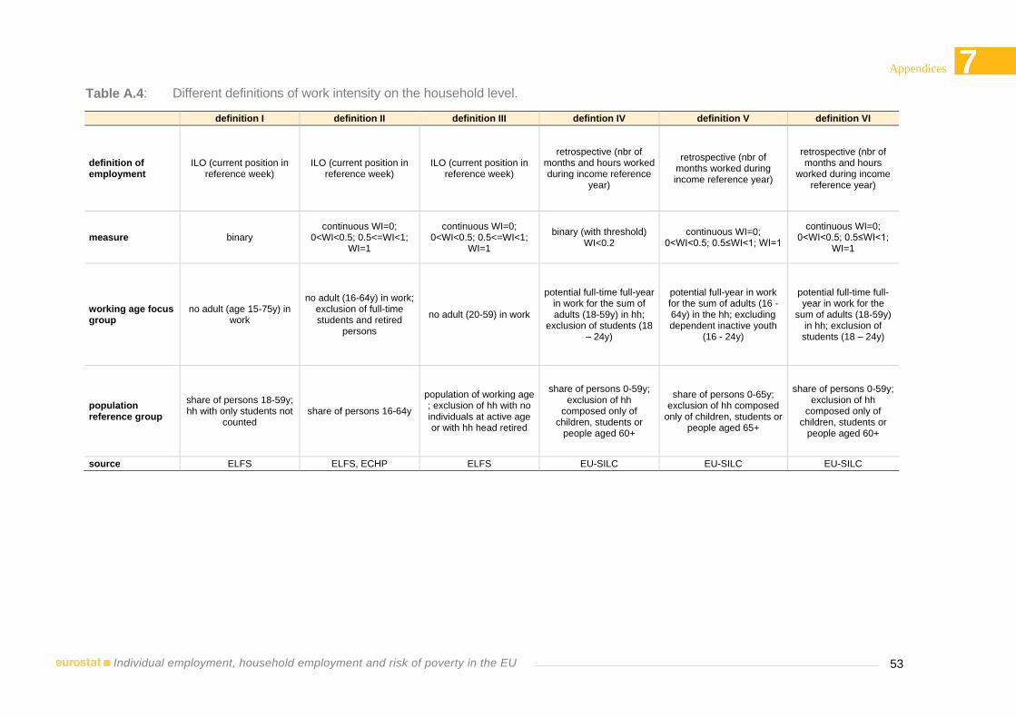
7 Appendices


Table A.4: Different definitions of work intensity on the household level.

definition I definition II definition III defintion IV definition V definition VI

definition of employment

ILO (current position in reference week)



retrospective (nbr of months and hours worked during income reference

year)

retrospective (nbr of months worked during income reference year)

retrospective (nbr of months and hours

worked during income reference year)

measure binary continuous WI=0;

0<WI<0.5; 0.5<=WI<1; WI=1

continuous WI=0; 0<WI<0.5; 0.5<=WI<1;

WI=1

binary (with threshold) WI<0.2

continuous WI=0; 0<WI<0.5; 0.5≤WI<1; WI=1

continuous WI=0; 0<WI<0.5; 0.5≤WI<1;

WI=1

working age focus group

no adult (age 15-75y) in work

no adult (16-64y) in work; exclusion of full-time students and retired

persons

no adult (20-59) in work

potential full-time full-year in work for the sum of adults (18-59y) in hh;

exclusion of students (18 – 24y)

potential full-year in work for the sum of adults (16 - 64y) in the hh; excluding dependent inactive youth

(16 - 24y)

potential full-time full-year in work for the

sum of adults (18-59y) in hh; exclusion of

students (18 – 24y)

population reference group

share of persons 18-59y; hh with only students not

counted share of persons 16-64y

population of working age ; exclusion of hh with no individuals at active age or with hh head retired

share of persons 0-59y; exclusion of hh

composed only of children, students or

people aged 60+

share of persons 0-65y; exclusion of hh composed

only of children, students or people aged 65+

share of persons 0-59y; exclusion of hh

composed only of children, students or

people aged 60+

source ELFS ELFS, ECHP ELFS EU-SILC EU-SILC EU-SILC

54

7 Appendices


Table A.5: Different definitions of work intensity at the household level, 2008.

country

Labour Force Survey Survey on Income and Living Conditions

def I definition II definition III def IV definition V definition VI

0 0 0 - 0.5 0.5 - 1 1 0 0 - 0.5 0.5 - 1 1 0 0 0 - 0.5 0.5 - 1 1 0 0 - 0.5 0.5 - 1 1

AT 7.8 11.4 3 24.7 61 8 1.3 23.1 67.6 7.8 12.2 6.9 37.2 43.7 6.8 8.9 54.6 29.7

BE 12.3 17.2 2.9 22.4 57.4 12.6 1.9 20.6 64.9 11.6 17.3 6.1 27.1 49.5 10 9 47.4 33.7

BG 8.6 12.9 3.7 27.1 56.2 9.4 2.5 22.6 65.5 8.1 10.5 12.4 40.8 36.4 5.8 14.8 39.4 40

CY 4.5 6.6 3.4 32.6 57.4 4.9 1.3 27.9 66 4.1 5.9 7.7 43.6 42.7 3.4 7.9 46.7 42

CZ 6 11 2 26.5 60.5 6.7 0.7 24.8 67.7 7.2 11.7 5.1 38.2 45 6.4 5 40.4 48.1

DE 10.8 13.8 1.8 20.7 63.7 11.6 0.8 21.2 66.4 11.7 15.9 3.7 27.7 52.7 10.4 7.4 53.2 29

DK 8.5 14.7 1.9 18.2 65.2 8 3.4 29.9 58.7

EE 5.9 9 1 20.8 69.1 7.7 0.7 18.8 72.8 5.3 7.9 3.3 33.4 55.4 4.4 4.5 39.8 51.4

EL 7.5 11.1 5.1 36.7 47.2 7.4 2.5 35.3 54.7 7.5 9.8 11.2 42.5 36.5 6.3 10.5 45.8 37.4

ES 6.5 8.6 7 38.8 45.6 7.7 3.9 35.5 52.9 6.1 8.5 7.7 42.2 41.6 4.6 9 50 36.5

FI 7.4 11.5 4.9 35.2 48.4 5.6 7.6 42.2 44.6

FR 10.2 15.1 1.5 22.8 60.6 10.2 0.7 21.4 67.6

HU 12.4 16.7 5.6 32.5 45.2 13.1 3.4 32 51.5 12.9 20.2 9.7 36.3 33.8 9.9 11.9 40.7 37.5

IE 8.7 10 2.8 30.6 56.6 10.4 1.6 29.3 58.7 13.7 13.8 8.7 38.3 39.3 11 14.5 50.1 24.5

IT 9.3 13.1 7.6 35.7 43.6 9.7 4.1 35.9 50.3 9.7 13.7 11.1 38 37.2 8.4 10.7 48.1 32.8

LT 9.1 11.6 2.6 22.8 63 9.6 1.8 19.7 69 5.1 8.3 5.3 32.4 54.1 4.5 6.2 35 54.2

LU 7.6 11.8 4.1 28.2 55.9 7.7 2.1 29.6 60.6 4.6 8.4 7.8 37.4 46.4 3.5 8.3 58.3 29.8

LV 5 7.4 6 37.2 49.3 4.2 7 40 48.8

NL 6.3 10.1 1.2 20 68.8 7.1 0.5 17.2 75.2 8.2 13.6 3.6 32.8 50 6.7 8.1 70 15.1

PL 10.3 13.1 7.7 33.7 45.5 10.3 4.9 31.2 53.6 7.9 13.8 9.4 40.3 36.5 6.1 10.9 47.6 35.4

PT 5.4 7.9 4.6 31 56.5 5.9 2.9 26.9 64.2 6.3 8.2 8.4 38.8 44.6 5.2 9.4 40.9 44.5

RO 10.1 12.3 6.4 32.7 48.7 10.7 4.1 30.9 54.3 8.4 12 9 37.6 41.4 7.4 10.2 40.2 42.2

SE 5.5 7.7 3.1 24.4 64.7 4.3 9.3 42.8 43.6

SI 6.7 10.1 5.1 25.7 59.1 6.3 2.3 22.3 69.1 6.7 11.7 8.2 35.6 44.5 5.9 5.9 34.1 54.1

SK 8.2 11.4 5.2 33.5 49.8 8.9 3.1 29.9 58.1 5 9.4 6 35.7 48.8 4.6 5 35.4 55

UK 14.3 12.9 1.5 20.3 65.3 12.6 0.8 18.2 68.3 10.3 13.1 1.7 19.8 65.4 8.8 7.6 48.4 35.1

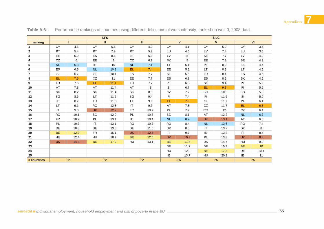
7 Appendices


Table A.6: Performance rankings of countries using different definitions of work intensity, ranked on wi = 0, 2008 data.

LFS SILC

ranking I II III IV V VI

1 CY 4.5 CY 6.6 CY 4.9 CY 4.1 CY 5.9 CY 3.4

2 PT 5.4 PT 7.9 PT 5.9 LU 4.6 LV 7.4 LU 3.5

3 EE 5.9 ES 8.6 SI 6.3 LV 5 SE 7.7 LV 4.2

4 CZ 6 EE 9 CZ 6.7 SK 5 EE 7.9 SE 4.3

5 NL 6.3 IE 10 NL 7.1 LT 5.1 PT 8.2 EE 4.4

6 ES 6.5 NL 10.1 EL 7.4 EE 5.3 LT 8.3 LT 4.5

7 SI 6.7 SI 10.1 ES 7.7 SE 5.5 LU 8.4 ES 4.6

8 EL 7.5 CZ 11 EE 7.7 ES 6.1 ES 8.5 SK 4.6

9 LU 7.6 EL 11.1 LU 7.7 PT 6.3 SK 9.4 PT 5.2

10 AT 7.8 AT 11.4 AT 8 SI 6.7 EL 9.8 FI 5.6

11 SK 8.2 SK 11.4 SK 8.9 CZ 7.2 BG 10.5 BG 5.8

12 BG 8.6 LT 11.6 BG 9.4 FI 7.4 FI 11.5 SI 5.9

13 IE 8.7 LU 11.8 LT 9.6 EL 7.5 SI 11.7 PL 6.1

14 LT 9.1 RO 12.3 IT 9.7 AT 7.8 CZ 11.7 EL 6.3

15 IT 9.3 UK 12.9 FR 10.2 PL 7.9 RO 12 CZ 6.4

16 RO 10.1 BG 12.9 PL 10.3 BG 8.1 AT 12.2 NL 6.7

17 FR 10.2 PL 13.1 IE 10.4 NL 8.2 UK 13.1 AT 6.8

18 PL 10.3 IT 13.1 RO 10.7 RO 8.4 NL 13.6 RO 7.4

19 DE 10.8 DE 13.8 DE 11.6 DK 8.5 IT 13.7 DK 8

20 BE 12.3 FR 15.1 UK 12.6 IT 9.7 IE 13.8 IT 8.4

21 HU 12.4 HU 16.7 BE 12.6 UK 10.3 PL 13.8 UK 8.8

22 UK 14.3 BE 17.2 HU 13.1 BE 11.6 DK 14.7 HU 9.9

23 DE 11.7 DE 15.9 BE 10

24 HU 12.9 BE 17.3 DE 10.4

25 IE 13.7 HU 20.2 IE 11

# countries 22 22 22 25 25 25

56

7 Appendices


Table A.7: Comparison of household joblessness indicators in LFS and SILC, 2008 data.

1 2 3 4 5 6 7 8

hhner (wi=0) - LFS wp (wi < 0.2) - SILC hhner (wi = 0) - SILC

Eurostat own

estimate Eurostat

own estimate

own estimate

AT 7 7.8 7.8 7.8 6.8 7.5 7.1 9.4

BE 12 12.3 11.7 11.6 10 11.2 10.8 13.1

BG 9 8.6 8.1 8.1 5.8 5.8 5.2 8

CY 4.9 4.5 4.1 4.1 3.4 3.8 2.9 4.1

CZ 6 6 7.2 7.2 6.4 6.5 6.2 7.5

DE 9 10.8 11.6 11.7 10.4 11.2 10.7 12

DK 8.3 8.5 8 9.6 9.3 10

EE 6.2 5.9 5.3 5.3 4.4 4.9 4.5 7.1

EL 7.5 7.5 7.4 7.5 6.3 7.2 6.3 7.7

ES 7.4 6.5 6.2 6.1 4.6 5.2 4.5 7.9

FI 7.3 7.4 5.6 6.7 6.4 10.3

FR 9.8 10.2 8.8

HU 12.5 12.4 12 12.9 9.9 10.5 10.4 14.1

IE 9 8.7 13.6 13.7 11 10.5 9.7 13.6

IT 9.6 9.3 9.8 9.7 8.4 9.4 8.7 10

LT 9 9.1 5.1 5.1 4.5 5.3 5 8.2

LU 7.9 7.6 4.7 4.6 3.5 3.9 3.8 5.5

LV 6.4 5.1 5 4.2 4.8 4.4 7.1

MT 8.2

NL 5.9 6.3 8.1 8.2 6.7 7.8 7.4 7

PL 10.1 10.3 7.9 7.9 6.1 7 6.7 13.6

PT 5.5 5.4 6.3 6.3 5.2 5.6 4.9 6.8

RO 10.5 10.1 8.2 8.4 7.4 8 7.7 8.9

SE 5.4 5.5 4.3 4.8 4.2 7.2

SI 6.4 6.7 6.7 6.7 5.9 7 6.8 8.3

SK 7.5 8.2 5.2 5 4.6 5.1 4.9 5.6

UK 10.7 14.3 10.4 10.3 8.8 7.4 7 13.7

57

7 7

Appendices 7 7

57


Figure A.5: Definition VI (EU2020), Distribution of population (0-59) by household work

intensity, 2009, SILC.

Figure A.6: Definition V (ISG, 2004), Distribution of population (0 – 59)(23) by household

work intensity, 2009, SILC.

(23) To improve comparability, age brackets for the population reference group are adapted to those of definition 6 (EU2020) .

0%

10%

20%

30%

40%

50%

60%

70%

80%

90%

100%

NL MT IE DE AT LU BE UK IT ES PL EL HU FR FI BG PT RO SE CY LV EE IS NO LT CZ SK SI DK

wi = 0 0 < wi <0.5 0.5 <= wi <1 wi = 1

0%

10%

20%

30%

40%

50%

60%

70%

80%

90%

100%

MT IE EL PL IT ES HU BG PT CY LV FI RO LU AT EE BE SK SI DE CZ LT FR NL IS SE NO DK UK

wi = 0 0 < wi <0.5 0.5 <= wi <1 wi = 1

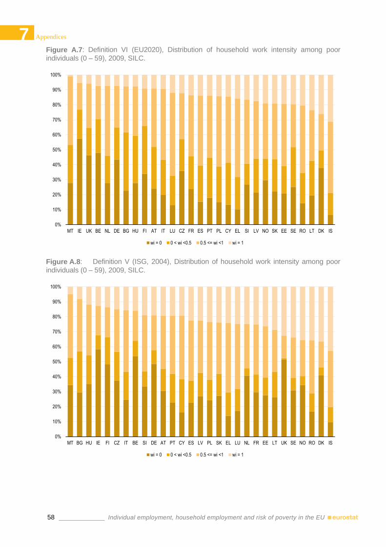
58

7 Appendices


Figure A.7: Definition VI (EU2020), Distribution of household work intensity among poor

individuals (0 – 59), 2009, SILC.

Figure A.8: Definition V (ISG, 2004), Distribution of household work intensity among poor

individuals (0 – 59), 2009, SILC.

0%

10%

20%

30%

40%

50%

60%

70%

80%

90%

100%

MT IE UK BE NL DE BG HU FI AT IT LU CZ FR ES PT PL CY EL SI LV NO SK EE SE RO LT DK IS

wi = 0 0 < wi <0.5 0.5 <= wi <1 wi = 1

0%

10%

20%

30%

40%

50%

60%

70%

80%

90%

100%

MT BG HU IE FI CZ IT BE SI DE AT PT CY ES LV PL SK EL LU NL FR EE LT UK SE NO RO DK IS

wi = 0 0 < wi <0.5 0.5 <= wi <1 wi = 1

59

7 7

Appendices 7 7

59


7.4 Appendix 4: Probability of joblessness on the individual level

In this section we further explore the socio-demographic characteristics of individuals who are confronted with a

high risk of living in a jobless household (ILO-concept) or a work-poor household with less than 50% work

intensity.

We estimate a probit model with a range of dependent socio-demographic covariates that may affect the

individual probability of living in a jobless (or work-poor) household. The probit model specifies a cumulative

distribution function of the standard normal distribution. The coefficients are estimated by maximum likelihood.

In a nonlinear model (as is the case with a binary dependent variable of household joblessness), marginal effects

are more informative than the coefficients. Therefore we provide estimates of the marginal effect at a benchmark

case.

In Table A. 8 and Table A. 9 we look at individual probabilities of household work intensity for the population

of six country clusters, for household joblessness (work intensity equals zero) and work-poor households (work

intensity is strictly lower than 0.5) respectively. In column 4 and 5 we compare old and new EU Member States

(EU15 versus EU10). In columns 6 to 9 the EU15 population is subdivided in four welfare state type clusters.

We provide both the estimated probability of household joblessness and the marginal effects of the different

covariates at the benchmark case of a 20-29 year old, unmarried low educated woman , born in an EU country,

who is not disabled and lives in a single adult household without children.

We find quite similar individual risks of living in a jobless or work-poor household for the reference individuals

in old and new EU member states. For the average working age adult (with the characteristics of the reference

individual - see column 3) the risk of household joblessness is 42.2 % and 47.1 %, for EU15 and EU10

respectively. The EU15 average conceals the lower household joblessness rate in Scandinavian countries and the

relatively high rate in Southern European countries.

But also the magnitude and sign of the marginal effects of the different socio-demographic characteristics for

both country clusters are largely similar. This social stratification reflects to a large extent some deep-rooted

social disadvantages with which individuals are born or have come to live with rather early on in their lives. First

of all and unsurprisingly, individuals with a high risk of living in a jobless household or a work-poor household

are individuals living in single households. This result is in part attributable to the mere ‘mathematical’ effect of

the absence of unemployment risk pooling in single households. With regard to the risk of living in a jobless

household, our age-result follows intuition. Compared with individuals aged 20-29, individuals between 30-54

face a lower risk and individuals between 55-59 face a significantly higher risk of living in a jobless household.

The result for the latter group is in line with what one would expect given early exit from the labour market.

Again, we find substantial differences by welfare state cluster. In Scandinavian countries there is no significant

difference in the probability of household joblessness for older and younger individuals. In Southern countries,

the youngest age group is at the highest risk. Rather surprisingly, having children does not influence the risk of

living in a jobless or work-poor household. Whatever the household size, we see that disabled individuals run a

higher risk of living in a jobless or work-poor household. Here the effect is stronger in older European Member

States countries, with a percentage point difference of 7.1. Moreover, the impact of individual educational

outcomes follows standard sociological relations; the lower the educational profile, the higher the probability of

living in a jobless household. Again, differences between EU15 and EU10 are limited, with the cluster of

Scandinavian countries displaying a divergent pattern with a limited positive effect of tertiary education on

household joblessness. Finally, the only socio-demographic characteristics for which the sign of the marginal

effect is opposite for different country clusters is origin (defined as country of birth). Being born in a non-

European country strongly increases the risk of living in a jobless household in Scandinavian and to a lesser

extent in Conservative European countries, but it decreases household joblessness in EU10 and liberal European

countries.

Using a more fine grained definition of household work intensity (see Table A. 9) slightly increases the risk of

household joblessness for the reference population. However, this effect is stronger in EU15 than in EU10,

which makes the gap in probabilities for both country clusters smaller. On the one hand, in Conservative and

Scandinavian countries the EU2020 estimation of living in a household with poor work intensity (with a

benchmark at 0.5) strongly increases the individual risk in comparison with the ILO definition (around 13

percentage points), while in Southern and liberal EU this change of definition increases the risk only slightly.

Considering the marginal effects, there are only subtle differences between the risk profiles of the two population

subgroups (jobless households, work-poor household) we distinguish here. The risks associated with age,

60

7 Appendices


education and disability are similar for joblessness and work poverty, yet the marginal effects of these individual

features are more important for work poverty than for joblessness (with some opposite effect within the welfare

state clusters). Also the impact of gender is more outspoken in the case of work poverty than in the case of

joblessness. A larger household size reduces the risk of joblessness and work poverty (compared to the risks of

singles), yet the reduction is relatively more important for a two-adult household when looking at work poverty

and relatively more important for a three-plus household when looking at joblessness.

Table A. 10 and Table A. 11 make a similar exercise, but expand the EU2020 definitions of work-poor

households with a peculiar focus on Belgium. In the covariates region is also added. The benchmark case is now

a 30-54 year old, unmarried, low educated woman, born in an EU country, who is not disabled and lives in a

single adult household without children in the Flemish region.

The first row of Table A. 10 shows the predicted probability for a working age adult (with the characteristics of

the reference case) of living in a jobless/ work-poor household. For the retrospective definition of full-time

employment in the reference year (EU2020) we use several benchmarks to define the household’s work poverty

(work intensity = 0; < 0.2; < 0.5; < 0.8). As already discussed in Appendix 2, the ILO definition of household

joblessness is less strict than the EU2020 definition. This explains why the probability of joblessness is higher

when the ILO definition is used. For the different benchmarks of work-poor households the risk of living in such

a household gradually increases from 35.4 per cent to 52.0 per cent in 2005. In 2008 those estimates are slightly

higher for all subgroups.

The magnitude of the marginal effects does gradually increase/decrease across the work-poor benchmarks. For

example, the negative impact of tertiary education on household joblessness decreases from -14.8 percentage

points to -25.6 percentage points. The same pattern can be found for gender, age and (very progressively) for

origin and disability. For the number of working age adults in the household the sign of the marginal effect turns

opposite for work rich households (benchmark between 0.5 and 0.8). At least one individual within the

household is not working full-time over the past year, which can be explained by risk pooling and time

management within the household. The effect of region and the impact of the presence of children in the

household do not gradually change with the narrowing of the definition of work-poorness. Living in Brussels

increases the risk for an individual of living in a work-poor household with around 8 percentage point in 2005,

independent of the applied benchmark for work intensity.

Table A. 11 estimates the probability of living in a jobless/work-poor household for individuals with specific

combinations of socio-demographic characteristics of gender, age and education and the number of working age

adults in the household. It is clear that for single adult households, the individual probability of living in a work-

poor household across different benchmarks does not differ as substantially as for the other household

composition types. For example, the estimated risk for a low educated, 55 – 59 year old single man differs from

0.78 of complete joblessness to 0.87 for work intensity lower than 0.8. For a man living in a household with two

working age adults this risk increases from 0.33 of complete joblessness to 0.88 for household work intensity 0

to 0.8. Within households with at least 2 working age adults, the gap in the individual risk is most outspoken

between work-poorness defined as smaller than 0.2 and smaller than 0.5. We conclude from this analysis that

both changes in household ‘joblessness’ (wp0) and in household ‘work poverty’ (wp0.5, work intensity less than

50%) may be interesting to understand the dynamics of poverty risks over time.

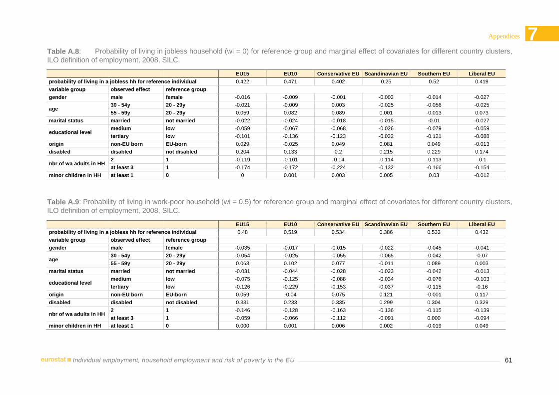
61

7 7 7

Appendices


Table A.8: Probability of living in jobless household (wi = 0) for reference group and marginal effect of covariates for different country clusters,

ILO definition of employment, 2008, SILC.

EU15 EU10 Conservative EU Scandinavian EU Southern EU Liberal EU

probability of living in a jobless hh for reference individual 0.422 0.471 0.402 0.25 0.52 0.419

variable group observed effect reference group

gender male female -0.016 -0.009 -0.001 -0.003 -0.014 -0.027

age 30 - 54y 20 - 29y -0.021 -0.009 0.003 -0.025 -0.056 -0.025

55 - 59y 20 - 29y 0.059 0.082 0.089 0.001 -0.013 0.073

marital status married not married -0.022 -0.024 -0.018 -0.015 -0.01 -0.027

educational level medium low -0.059 -0.067 -0.068 -0.026 -0.079 -0.059

tertiary low -0.101 -0.136 -0.123 -0.032 -0.121 -0.088

origin non-EU born EU-born 0.029 -0.025 0.049 0.081 0.049 -0.013

disabled disabled not disabled 0.204 0.133 0.2 0.215 0.229 0.174

nbr of wa adults in HH 2 1 -0.119 -0.101 -0.14 -0.114 -0.113 -0.1

at least 3 1 -0.174 -0.172 -0.224 -0.132 -0.166 -0.154

minor children in HH at least 1 0 0 0.001 0.003 0.005 0.03 -0.012

Table A.9: Probability of living in work-poor household (wi = 0.5) for reference group and marginal effect of covariates for different country clusters,

ILO definition of employment, 2008, SILC.

EU15 EU10 Conservative EU Scandinavian EU Southern EU Liberal EU

probability of living in a jobless hh for reference individual 0.48 0.519 0.534 0.386 0.533 0.432

variable group observed effect reference group

gender male female -0.035 -0.017 -0.015 -0.022 -0.045 -0.041

age 30 - 54y 20 - 29y -0.054 -0.025 -0.055 -0.065 -0.042 -0.07

55 - 59y 20 - 29y 0.063 0.102 0.077 -0.011 0.089 0.003

marital status married not married -0.031 -0.044 -0.028 -0.023 -0.042 -0.013

educational level medium low -0.075 -0.125 -0.088 -0.034 -0.076 -0.103

tertiary low -0.126 -0.229 -0.153 -0.037 -0.115 -0.16

origin non-EU born EU-born 0.059 -0.04 0.075 0.121 -0.001 0.117

disabled disabled not disabled 0.331 0.233 0.335 0.299 0.304 0.329

nbr of wa adults in HH 2 1 -0.146 -0.128 -0.163 -0.136 -0.115 -0.139

at least 3 1 -0.059 -0.066 -0.112 -0.091 0.000 -0.094

minor children in HH at least 1 0 0.000 0.001 0.006 0.002 -0.019 0.049

62

7 Appendices


Table A.10: Probability of living in jobless/ work-poor household for reference group and marginal effect of covariates for different definitions of

work intensity (ILO, EU2020 with gradual benchmark), Belgium, 2005 & 2008, SILC.

2005 2008

ilo eu2020 ilo eu2020

jl jl wi < 0.2 wi < 0.5 wi < 0.8 jl jl wi < 0.2 wi < 0.5 wi < 0.8

Probability of living in jl/wp hh for reference individual 0.399 0.354 0.371 0.43 0.52 0.469 0.394 0.428 0.483 0.557

variable observed effect reference group

gender male female -0.038 -0.035 -0.044 -0.05 -0.069 -0.025 -0.02 -0.025 -0.042 -0.049

age 20 - 29y 30 - 54y 0.024 0.021 0.034 0.048 0.045 0.009 0.007 0.014 0.013 0.021

55 - 59y 30 - 54y 0.173 0.142 0.154 0.202 0.275 0.125 0.101 0.118 0.156 0.262

marital status married not married -0.011 -0.022 -0.024 -0.028 0.033 -0.007 0.008 -0.007 -0.024 0.055

educational level medium low -0.076 -0.07 -0.076 -0.096 -0.147 -0.101 -0.077 -0.089 -0.124 -0.165

tertiary low -0.15 -0.148 -0.157 -0.18 -0.256 -0.172 -0.142 -0.162 -0.215 -0.298

region Brussels region Flemish region 0.077 0.069 0.078 0.088 0.071 0.034 0.034 0.039 0.063 0.042

Walloon region Flemish region 0.061 0.072 0.077 0.059 0.072 0.053 0.053 0.052 0.062 0.064

origin non-EU born EU-born 0.095 0.075 0.084 0.149 0.188 0.114 0.094 0.115 0.168 0.223

disabled disabled not disabled 0.234 0.206 0.223 0.303 0.669 0.158 0.144 0.167 0.244 0.421

nbr of wa adults in HH

2 1 -0.139 -0.121 -0.126 -0.146 0.062 -0.156 -0.155 -0.153 -0.139 0.013

at least 3 1 -0.225 -0.207 -0.193 -0.035 0.312 -0.212 -0.197 -0.183 -0.058 0.188

minor children in HH at least 1 0 -0.021 -0.013 -0.011 -0.027 -0.02 -0.021 -0.02 -0.019 -0.047 -0.025

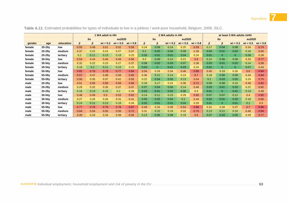
63

7 7 7

Appendices


Table A.11: Estimated probabilities for types of individuals to live in a jobless / work-poor household, Belgium, 2008, SILC.

1 WA adult in HH 2 WA adults in HH at least 3 WA adults inHH

ilo eu2020 ilo eu2020 ilo eu2020

gender age education jl jl wi < 0.2 wi < 0.5 wi < 0.8 jl jl wi < 0.2 wi < 0.5 wi < 0.8 jl jl wi < 0.2 wi < 0.5 wi < 0.8

female 20-29y low 0.55 0.48 0.51 0.52 0.59 0.24 0.09 0.14 0.25 0.59 0.17 0.04 0.08 0.34 0.74

female 20-29y medium 0.37 0.22 0.24 0.27 0.37 0.1 0.02 0.04 0.09 0.38 0.04 0.01 0.02 0.16 0.55

female 20-29y tertiary 0.2 0.11 0.13 0.18 0.25 0.05 0.01 0.01 0.04 0.24 0.01 0 0 0.08 0.39

female 30-54y low 0.53 0.44 0.46 0.49 0.56 0.2 0.09 0.12 0.21 0.6 0.12 0.06 0.09 0.33 0.77

female 30-54y medium 0.32 0.22 0.23 0.27 0.37 0.08 0.02 0.03 0.07 0.38 0.03 0.01 0.02 0.14 0.59

female 30-54y tertiary 0.18 0.1 0.11 0.15 0.23 0.03 0 0.01 0.03 0.24 0.01 0 0 0.07 0.44

female 55-59y low 0.82 0.76 0.78 0.77 0.84 0.54 0.29 0.34 0.46 0.85 0.45 0.19 0.26 0.6 0.94

female 55-59y medium 0.67 0.47 0.48 0.49 0.65 0.36 0.11 0.14 0.24 0.7 0.18 0.06 0.09 0.34 0.84

female 55-59y tertiary 0.56 0.35 0.37 0.41 0.55 0.22 0.04 0.05 0.13 0.54 0.1 0.03 0.05 0.24 0.75

male 20-29y low 0.51 0.55 0.59 0.59 0.66 0.18 0.17 0.24 0.36 0.71 0.09 0.08 0.15 0.46 0.82

male 20-29y medium 0.29 0.32 0.35 0.37 0.47 0.07 0.04 0.06 0.14 0.46 0.03 0.01 0.03 0.22 0.62

male 20-29y tertiary 0.16 0.13 0.15 0.2 0.28 0.03 0.01 0.02 0.06 0.3 0.01 0 0.01 0.13 0.48

male 30-54y low 0.48 0.49 0.5 0.53 0.62 0.14 0.11 0.15 0.26 0.65 0.07 0.07 0.12 0.4 0.82

male 30-54y medium 0.27 0.25 0.26 0.31 0.41 0.05 0.03 0.04 0.1 0.44 0.02 0.01 0.03 0.18 0.65

male 30-54y tertiary 0.14 0.11 0.13 0.18 0.26 0.02 0.01 0.01 0.04 0.29 0.01 0 0.01 0.1 0.5

male 55-59y low 0.77 0.78 0.79 0.78 0.87 0.49 0.33 0.39 0.53 0.88 0.31 0.28 0.37 0.7 0.96

male 55-59y medium 0.64 0.54 0.55 0.56 0.72 0.31 0.15 0.19 0.32 0.75 0.13 0.11 0.16 0.46 0.89

male 55-59y tertiary 0.49 0.33 0.34 0.39 0.56 0.13 0.06 0.08 0.18 0.6 0.07 0.03 0.05 0.29 0.77

European Commission

Individual employment, household employment and risk of poverty in the EU. A decomposition analysis Luxembourg: Publications Office of the European Union 2013 — 63 pp. — 21 x 29.7 cm ISBN 978-92-79-29045-9 ISSN 1977-0375 doi:10.2785/41846 Cat. No KS-RA-13-014-EN-N Theme: Populations and social conditionsCollection: Methodologies & Working papers

HOW TO OBTAIN EU PUBLICATIONS Free publications: • via EU Bookshop (http://bookshop.europa.eu);

• at the European Union’s representations or delegations. You can obtain their contact details on the Internet (http://ec.europa.eu) or by sending a fax to +352 2929-42758.

Priced publications: • via EU Bookshop (http://bookshop.europa.eu).

Priced subscriptions (e.g. annual series of the Official Journal of the European Union and reports of cases before the Court of Justice of the European Union): • via one of the sales agents of the Publications Office of the European Union

(http://publications.europa.eu/others/agents/index_en.htm)

http://bookshop.europa.eu

http://ec.europa.eu

http://bookshop.europa.eu

http://publications.europa.eu/others/agents/index_en.htm

2008 edition

KS-RA-13-014-EN

-N


Domestic tourism manual

ISSN 1977-0375

individual employment, household employment and risk of

Documents