independent introductions and admixtures have contributed to

RESEARCH ARTICLE

Independent introductions and admixtures

have contributed to adaptation of European

maize and its American counterparts

Jean-Tristan Brandenburg1, Tristan Mary-Huard1,2, Guillem Rigaill3, Sarah J. Hearne4,

Helène Corti1, Johann Joets1, Clementine Vitte1, Alain Charcosset1, Stephane D. Nicolas1,

Maud I. Tenaillon1*

1 Genetique Quantitative et Evolution – Le Moulon, Institut National de la Recherche agronomique,

Universite Paris-Sud, Centre National de la Recherche Scientifique, AgroParisTech, Universite Paris-Saclay,

France, 2 UMR 518 AgroParisTech/INRA, France, 3 Institute of Plant Sciences Paris-Saclay, UMR 9213/

UMR1403, CNRS, INRA, Universite Paris-Sud, Universite d’Evry, Universite Paris-Diderot, Sorbonne Paris-

Cite, France, 4 CIMMYT (International Maize and Wheat Improvement Centre), El Batan, Texcoco, Edo de

Mexico, Mexico

* [email protected]

Abstract

Through the local selection of landraces, humans have guided the adaptation of crops to a

vast range of climatic and ecological conditions. This is particularly true of maize, which was

domesticated in a restricted area of Mexico but now displays one of the broadest cultivated

ranges worldwide. Here, we sequenced 67 genomes with an average sequencing depth of

18x to document routes of introduction, admixture and selective history of European maize

and its American counterparts. To avoid the confounding effects of recent breeding, we tar-

geted germplasm (lines) directly derived from landraces. Among our lines, we discovered

22,294,769 SNPs and between 0.9% to 4.1% residual heterozygosity. Using a segmenta-

tion method, we identified 6,978 segments of unexpectedly high rate of heterozygosity.

These segments point to genes potentially involved in inbreeding depression, and to a

lesser extent to the presence of structural variants. Genetic structuring and inferences of

historical splits revealed 5 genetic groups and two independent European introductions,

with modest bottleneck signatures. Our results further revealed admixtures between distinct

sources that have contributed to the establishment of 3 groups at intermediate latitudes in

North America and Europe. We combined differentiation- and diversity-based statistics to

identify both genes and gene networks displaying strong signals of selection. These include

genes/gene networks involved in flowering time, drought and cold tolerance, plant defense

and starch properties. Overall, our results provide novel insights into the evolutionary history

of European maize and highlight a major role of admixture in environmental adaptation, par-

alleling recent findings in humans.

PLOS Genetics | https://doi.org/10.1371/journal.pgen.1006666 March 16, 2017 1 / 30

a1111111111

a1111111111

a1111111111

a1111111111

a1111111111

OPENACCESS

Citation: Brandenburg J-T, Mary-Huard T, Rigaill

G, Hearne SJ, Corti H, Joets J, et al. (2017)

Independent introductions and admixtures have

contributed to adaptation of European maize and

its American counterparts. PLoS Genet 13(3):

e1006666. https://doi.org/10.1371/journal.

pgen.1006666

Editor: Nathan M. Springer, University of

Minnesota, UNITED STATES

Received: July 5, 2016

Accepted: March 1, 2017

Published: March 16, 2017

Copyright: © 2017 Brandenburg et al. This is an

open access article distributed under the terms of

the Creative Commons Attribution License, which

permits unrestricted use, distribution, and

reproduction in any medium, provided the original

author and source are credited.

Data Availability Statement: DNA-sequencing

reads from all lines were deposited in the European

Nucleotide Archive (ENA) under the study

accession number PRJEB14212.

Funding: This work was supported by the French

National Research Agency (ANR) as part of the

“Investissements d’Avenir” Programme (Amaizing;

ANR-10-BTBR-03, AMAIZING, France Agrimer).

JTB was successively funded by the

“Investissements d’Avenir” Programme, the LabEx

https://doi.org/10.1371/journal.pgen.1006666

http://crossmark.crossref.org/dialog/?doi=10.1371/journal.pgen.1006666&domain=pdf&date_stamp=2017-03-30








http://creativecommons.org/licenses/by/4.0/

Author summary

The spread of a species outside its native range depends on its ability to face new environ-

mental challenges. Despite a loss of diversity associated with recurrent introductions,

domesticated species offer excellent examples of rapid expansion and adaptation to new

climatic and ecological conditions. This is exemplified in maize, which was first domesti-

cated in a restricted area of Central Mexico but now displays one of the broadest cultivated

ranges of all crops. Here, we focused on the largely overlooked history of European maize,

which was introduced from American sources. We sequenced 67 genomes from both con-

tinents. The data suggest two independent European introductions and also the admixed

origin of three groups: maize from the US Corn Belt, European Flints and Italian material.

We found modest genetic footprints of bottlenecks from European introduction. We

detected signs of past selection at genes and gene pathways involved in adaptation to abi-

otic (drought/cold) and biotic (pathogens/herbivores) challenges. Our results provide

novel insights into the evolutionary history of European maize and highlight a major role

of admixture in environmental adaptation.

Introduction

Expansion of species to conditions that differ from their native range depends on their abilities

to adapt to new environments. Depletion of genetic diversity of introduced—founder—popula-

tions may however alter this ability. Despite loss of diversity associated with population bottle-

necks during their domestication [1], domesticated species offer repeated examples of shifts in

geographic range. There is in fact little overlap between the centers of origin of major crops and

their area of highest production in the modern world [2]. For example, niche modeling of prim-

itive maize landraces and cotton cultivars has demonstrated that their range rapidly exceeds

that of their wild relatives [3,4]. Such rapid expansion is facilitated along east-west axes sharing

more similar day-length characteristics and climates than along north-south axes [2]. Accord-

ingly, data suggest that the evolution of vernalization or photoperiod-neutral requirements has

delayed expansion of wheat and barley to Northern latitudes by hundreds of years [5].

In plants, while numerous studies have documented the early demographic and selective

history of domesticated plants [6,7], a handful has focused on the routes of migration of crops

outside their native range. It is clear, however, that migration routes and subsequent admix-

tures are important drivers of adaptation. For instance, adaptation of Tibetan highlanders

to hypoxic conditions was facilitated through introgressions from individuals of Denisovan

ancestry [8]. Similarly, introgressions from Neanderthal have contributed to functional adap-

tive variation at innate immunity genes in modern European populations [9]. In this study, we

propose to address these issues in maize, a prime example of crop adaptive success displaying

one of the broadest cultivated range.

Maize was domesticated around 9,000 BP in the tropical lowlands of Mexico [10,11].

Domestication and breeding bottlenecks in the Americas have reduced genetic diversity by

20% and<5% respectively [12]. Spread of maize landraces throughout the American continent

has been addressed by earlier studies showing two major expansions northwards and south-

wards from Mexico [13]. In contrast with the well-established history of American maize, the

history of European maize has been largely overlooked (reviewed in [14]). Two molecular

studies, based on a restricted set of markers, have converged on the following conclusions.

First, introductions to Europe occurred soon after the discovery of the Americas by Columbus.

Second, landraces from northern Europe are related to northern American landraces, while

Evolutionary genomics of European and American maize


BASC (ANR-11-LABX-0034) as well as the Institut

Diversite, Ecologie et Evolution du Vivant (IDEEV).

Double Haploids from CIMMYT were developed

under the MasAgro (Sustainable Modernization of

Traditional Agriculture) initiative supported by

SAGARPA (La secretaria de Agricultura, Ganaderia,

Desarollo Rural, Pesca y Alimentacion), Mexico.

The funders had no role in study design, data

collection and analysis, decision to publish, or

preparation of the manuscript.

Competing interests: The authors have declared

that no competing interests exist.


landraces from southern Europe are related to Tropical lowland maize, which are of Caribbean

origin [15]. Third, paralleling the emergence of the Corn Belt Dents at mid-latitudes in the

US, the European Flints may derive from admixture between European northern and southern

material [15,16].

Previous studies have genotyped maize from the Americas with MaizeSNP50k genotyping

array [17], Genotype-by-Sequencing technology [18,19], or low-depth (5x) whole-genome

sequencing [20] to detect genomic regions targeted by selection at the species level. More

recently, Unterseer and colleagues [21] have undertaken an alternative approach by contrast-

ing lines from two temperate heterotic groups (Dents and Flints) to screen for breeding signals

using the MaizeSNP600k array that targets about half of maize annotated genes. Those studies

have collectively identified hundreds of putative genomic targets of selection during ancient

and more recent breeding history—in traditional landraces and elite maize lines. The pheno-

typic impact of a handful of genes has been validated through linkage-based cloning and

association mapping, among which ZmCCT has been shown to contribute to day-length adap-

tation [22], and Vgt1 [23] and ZCN8 [24] are associated with flowering time. Because of the

rapid decline of linkage disequilibrium in maize [1], a high density of markers is necessary to

address a more complete inventory of genomic targets.

To document routes of introduction, patterns of admixture and the selective history of

European corn and its American counterparts, we performed whole-genome sequencing of 67

maize lines from the two continents at mid-depth (18x). We purposely sampled inbred lines

directly derived from landraces both to avoid the confounding effects of recent breeding selec-

tion and to account for geographical information. With >22 million SNPs identified, we (1)

describe the genome-wide distribution of heterozygosity along chromosomes, (2) assess pro-

posed sources of European maize, (3) measure the impact of introduction bottlenecks, (4)

explore admixture events, (5) track signatures of selection at the level of genes and gene net-

works, using latitudinal and longitudinal contrasts.

Results

With the purpose of tracing the origins of European maize and investigating its demographic

and selective history, we combined genetic, historic and geographic information to select a

sample of 67 maize lines. This sample is representative of European maize diversity and

encompasses all possible American introduction sources. We specifically targeted lines directly

derived from traditional populations (landraces), for which we have established the geographic

origin from historical records. Such lines are less heterozygous than landraces and therefore

more amenable for high-throughput sequencing (HTS) genotype calls. They are also less

affected by recent and intense selection than elite lines, and therefore particularly relevant for

conducting population genomic analyzes with a historical perspective.

Altogether our sample included 48 first-cycle maize inbred lines, 9 lines obtained by single

seed descent and 10 doubled haploids. The lines covered 11 major groups described in previ-

ous studies [13,25] and thus defined here a priori (Fig 1A, S1 Table). These eleven groups are

the American (n = 5) and European (n = 8) Northern Flints (ANFs and ENFs), which we

collectively call the Northern Flints, European Flints (EFs, n = 13), Spanish (n = 3), Italians

(n = 5), Mexican lowlands (n = 5) and highlands (n = 2), Caribbeans (n = 5), Southern (n = 5)

and Northern South Americans (n = 2), and Corn Belt Dents (CBDs, n = 14).

Polymorphism discovery and accuracy of genotype calling

We generated 2x100 bases paired-end reads from High Throughput Sequencing (HTS) of 67

lines totaling 2,654 Gb of sequences. We aligned them to the B73 v2 reference genome [26].




The percentage of paired-end reads mapped with correct insert sizes ranged between 68.2%

and 80.1%, depending on the line (S1 Table). Considering only bases covered by at least 4

reads (4x depth), the per-line reference genome coverage varied between 70.3% and 78.6%

(S1 Fig).

The maize genome has undergone several rounds of duplications and contains large pro-

portions (85%) of transposable elements [26]. This genomic redundancy makes polymorphism

calling a challenging task. In particular, misalignment of paralogous regions often causes het-

erozygotes miscalling. We designed customized filters to increase the accuracy of SNP calling.

A small proportion of positions called by Varscan (~16%) passed these filters. Among posi-

tions that we discarded: ~30% contained > 50% of missing data; ~30% became monomorphic

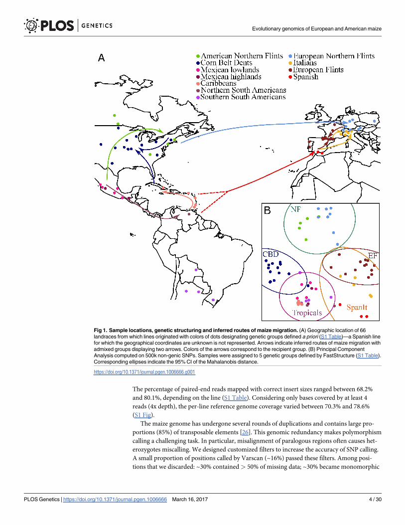
Fig 1. Sample locations, genetic structuring and inferred routes of maize migration. (A) Geographic location of 66

landraces from which lines originated with colors of dots designating genetic groups defined a priori (S1 Table)—a Spanish line

for which the geographical coordinates are unknown is not represented. Arrows indicate inferred routes of maize migration with

admixed groups displaying two arrows. Colors of the arrows correspond to the recipient group. (B) Principal Component

Analysis computed on 500k non-genic SNPs. Samples were assigned to 5 genetic groups defined by FastStructure (S1 Table).

Corresponding ellipses indicate the 95% CI of the Mahalanobis distance.

https://doi.org/10.1371/journal.pgen.1006666.g001





after filtering for read-depth variation, multiple mapping, and genotype uncertainties (LRT

not significant); and another ~40% were suspected to belong to duplicated regions based on

error count, heterozygotes count, elevated read-depth variation and/or proportion of multiple

mapped reads.

We obtained a dataset of 22,294,769 Single Nucleotide Polymorphisms (SNPs) after filter-

ing, of which 86.0% were located outside genes, 5.4% in exonic regions and 8.6% in intronic

regions. In total 34,350 out of the 39,423 genes of the maize genome were covered by at least

one SNP. The percentage of missing data per line ranged between 18.2% and 32.1% (S2 Fig).

2,189,230 (9.8%) SNPs encompassed no missing data. Given genome divergence between spe-

cies, we were able to map only 6.19% of HTS data from Tripsacum dactyloides [20] to the B73

v2 reference genome. In total, we managed to orientate 1,255,761 of our SNPs with Tripsacumdactyloides, half of which (48.5%) were located in genic regions.

Proportion of heterozygous sites (SNPs x lines) was initially comprised between 26.5% and

37.5%, but decreased after filtering to a range of 0.9% to 4.1% (S1 Table). To test the efficiency

of our filters to remove false heterozygotes, which are often confounded with homozygous alle-

lic variants at duplicated sites, we compared the average heterozygous sites proportion across

lines between a set of genes encompassing paralogs (2,788 genes) and a set of single genes with

no paralogous copy (3,949 genes) [27]. We found no significant difference between the two

sets with a two-sided Kolmogorov-Smirnov test (P-value = 0.873), thus indicating that gene

paralogy is well accounted for heterozygous calls.

We further estimated miscalling of both homozygotes and heterozygotes by comparing

our HTS genotype calling to that obtained with the MaizeSNP50k genotyping array (S1 Table,

~38,000 positions analyzed). We found a rate of discrepancy between the two datasets that ran-

ged from 0.016% to 0.21% per line—with an average value of 0.038% across lines. For a subset

of 20 lines (S1 Table), our MaizeSNP50k and HTS genotypes were obtained from the same

DNA extractions. Considering this subset, the error rate of genotype calling in our HTS data

for homozygotes dropped to 0.036%. In contrast, for heterozygotes (181 positions on average

per individual), the percentage of false negatives—proportion of homozygotes in our HTS data

among heterozygotes in the MaizeSNP50k data—and false positives—proportion of false het-

erozygotes among heterozygotes in our HTS data—was 18.3% and 34% respectively.

Finally, we assessed the power of our HTS approach over MaizeSNP50k SNP to analyze

maize genetic diversity by comparing folded Site Frequency Spectra (S3 Fig). The two SFS dif-

fered markedly, pointing to a marked deficit of rare variants in the array data. Such a deficit is

expected, because a restricted panel of lines was used for SNP discovery for the MaizeSNP50k

SNP design.

In sum, our HTS approach combined multiple advantages: high SNP density; a low error

rate for homozygous calls; and a realistic description of allele frequencies, including low fre-

quency variants that are likely to have arisen recently and are therefore informative for assess-

ing both recent ancestry and selection.

Patterns of genetic diversity reveals a complex demographic history

In order to get insights into the history of divergence and admixtures in our sample, we

applied Treemix to the 11 groups that were defined a priori (S1 Table), using Tripsacum dacty-loides as an outgroup. The corresponding unfolded SFS is shown in S4 Fig. As illustrated in Fig

2, our results showed: (1) a major split isolating Northern Flints and European Flints from the

rest; the marked distinction of NFs from ancestral Mexican lines was confirmed by elevated

Fst values between NFs and all other groups (S2 Table); (2) proximity of NFs and EFs, the latter

being admixed by ancestors of the Southern European Material; (3) an admixed origin of the




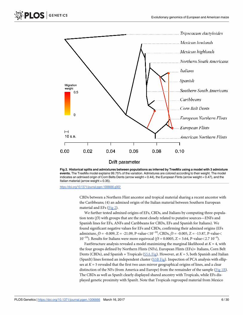
CBDs between a Northern Flint ancestor and tropical material sharing a recent ancestor with

the Caribbeans; (4) an admixed origin of the Italian material between Southern European

material and EFs (Fig 2).

We further tested admixed origins of EFs, CBDs, and Italians by computing three-popula-

tion tests (f3) with groups that are the most closely related to putative sources—ENFs and

Spanish lines for EFs, ANFs and Caribbeans for CBDs, EFs and Spanish for Italians). We

found significant negative values for EFs and CBDs, confirming their admixed origins (EFs

admixture, f3 = -0.009, Z = -21.09, P-value<10−10; CBDs, f3 = -0.005, Z = -13.87, P-value<

10−10). Results for Italians were more equivocal (f3 = 0.0005, Z = 3.64, P-value<2.7 10−4).

FastStructure analysis revealed a model maximizing the marginal likelihood at K = 4, with

the four groups defined by Northern Flints (NFs), European Flints (EFs)+ Italians, Corn Belt

Dents (CBDs), and Spanish + Tropicals (S5A Fig). However, at K = 5, both Spanish and Italian

(SpanIt) lines formed an independent cluster (S5B Fig). Inspection of PCA analysis with ellip-

ses at K = 5 revealed that the first two axes mirror geographical origins of lines, and a clear

distinction of the NFs (from America and Europe) from the remainder of the sample (Fig 1B).

The CBDs as well as SpanIt clearly displayed shared ancestry with Tropicals, while EFs dis-

played genetic proximity with SpanIt. Note that Tropicals regrouped material from Mexico

Fig 2. Historical splits and admixtures between populations as inferred by TreeMix using a model with 3 admixture

events. The TreeMix model explains 99.75% of the variation. Admixtures are colored according to their weight. The model

indicates an admixed origin of Corn Belts Dents (arrow weight = 0.44), the European Flints (arrow weight = 0.47), and the

Italian material (arrow weight = 0.35).






(lowlands and highlands), South America (northern and southern) and Caribbeans. Grouping

of Tropicals was further supported by extremely low Fst values (<0.05), with an average Fst

of 0.02 within Tropicals, i.e. average value obtained from all pairwise comparisons involving

material from Mexico, South America, and Caribbeans as listed above. In comparison, we

obtained an average Fst of 0.15 when comparing Tropicals to all other groups (S2 Table).

We estimated genome-wide nucleotide diversity (π/bp) of the non-genic compartment for

the 5 genetic groups: Tropicals displayed the highest level of genetic diversity of all 5 groups

(0.00824, n = 19), followed by EFs (0.00739, n = 13), CBDs (0.00736, n = 14), SpanIt (0.00694,

n = 8), and NFs (0.00648, n = 13). Distributions of nucleotide diversity for all genetic groups

are shown in S6 Fig.

Finally, we performed a more detailed inspection of admixture of CBDs and EFs using Fas-

tStructure. While American Northern Flints contributed less to the CBDs than the Tropicals

(S7A Fig), the contribution of NFs and Southern European material to the EFs was balanced

(S7B Fig).

Footprints of European introductions

One of our main goals was to test whether introductions of European corn were associated

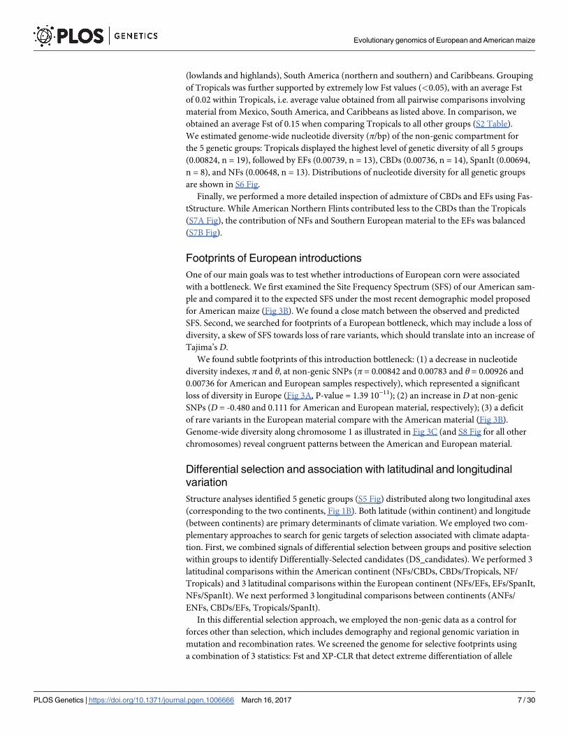
with a bottleneck. We first examined the Site Frequency Spectrum (SFS) of our American sam-

ple and compared it to the expected SFS under the most recent demographic model proposed

for American maize (Fig 3B). We found a close match between the observed and predicted

SFS. Second, we searched for footprints of a European bottleneck, which may include a loss of

diversity, a skew of SFS towards loss of rare variants, which should translate into an increase of

Tajima’s D.

We found subtle footprints of this introduction bottleneck: (1) a decrease in nucleotide

diversity indexes, π and θ, at non-genic SNPs (π = 0.00842 and 0.00783 and θ = 0.00926 and

0.00736 for American and European samples respectively), which represented a significant

loss of diversity in Europe (Fig 3A, P-value = 1.39 10−11); (2) an increase in D at non-genic

SNPs (D = -0.480 and 0.111 for American and European material, respectively); (3) a deficit

of rare variants in the European material compare with the American material (Fig 3B).

Genome-wide diversity along chromosome 1 as illustrated in Fig 3C (and S8 Fig for all other

chromosomes) reveal congruent patterns between the American and European material.

Differential selection and association with latitudinal and longitudinal

variation

Structure analyses identified 5 genetic groups (S5 Fig) distributed along two longitudinal axes

(corresponding to the two continents, Fig 1B). Both latitude (within continent) and longitude

(between continents) are primary determinants of climate variation. We employed two com-

plementary approaches to search for genic targets of selection associated with climate adapta-

tion. First, we combined signals of differential selection between groups and positive selection

within groups to identify Differentially-Selected candidates (DS_candidates). We performed 3

latitudinal comparisons within the American continent (NFs/CBDs, CBDs/Tropicals, NF/

Tropicals) and 3 latitudinal comparisons within the European continent (NFs/EFs, EFs/SpanIt,

NFs/SpanIt). We next performed 3 longitudinal comparisons between continents (ANFs/

ENFs, CBDs/EFs, Tropicals/SpanIt).

In this differential selection approach, we employed the non-genic data as a control for

forces other than selection, which includes demography and regional genomic variation in

mutation and recombination rates. We screened the genome for selective footprints using

a combination of 3 statistics: Fst and XP-CLR that detect extreme differentiation of allele




frequencies between groups (the latter accounting for local linkage disequilibrium), and D that

detects selection within a group. Genes passing the 5% threshold for all 3 statistics were consid-

ered as candidate genes.

Among 9 pairwise comparisons (Table 1) we detected 968 DS_candidate genes (S3 Table),

and 252 of them were involved in multiple comparisons. That a given gene was involved in

multiple comparisons was mainly caused by a given group being used in multiple comparisons

rather than a signal of convergent selection between comparisons using distinct groups. The

number of DS_ candidates varied between 46 and 219 (Table 1) among comparisons, with

the CBDs and Tropicals comparisons offering the smallest number of candidates. On average,

Fig 3. Genome-wide patterns of nucleotide diversity of American and European samples. A: Box-plots of non-genic

per-bp nucleotide diversity (π) estimated on 4,799 non-overlapping segments of 10kb along the genome. B: Folded Site

Frequency Spectra of the European sample and the American sample projected down to 29 samples. SFS were built on a

common set of 2,941,528 non-genic SNPs. SFS expectation for American landraces from a model incorporating a

domestication bottleneck, population expansion and gene flow (parameters from [28]) is shown by a red line. C: Variation of

π/bp along chromosome 1 computed from 50kb sliding windows.






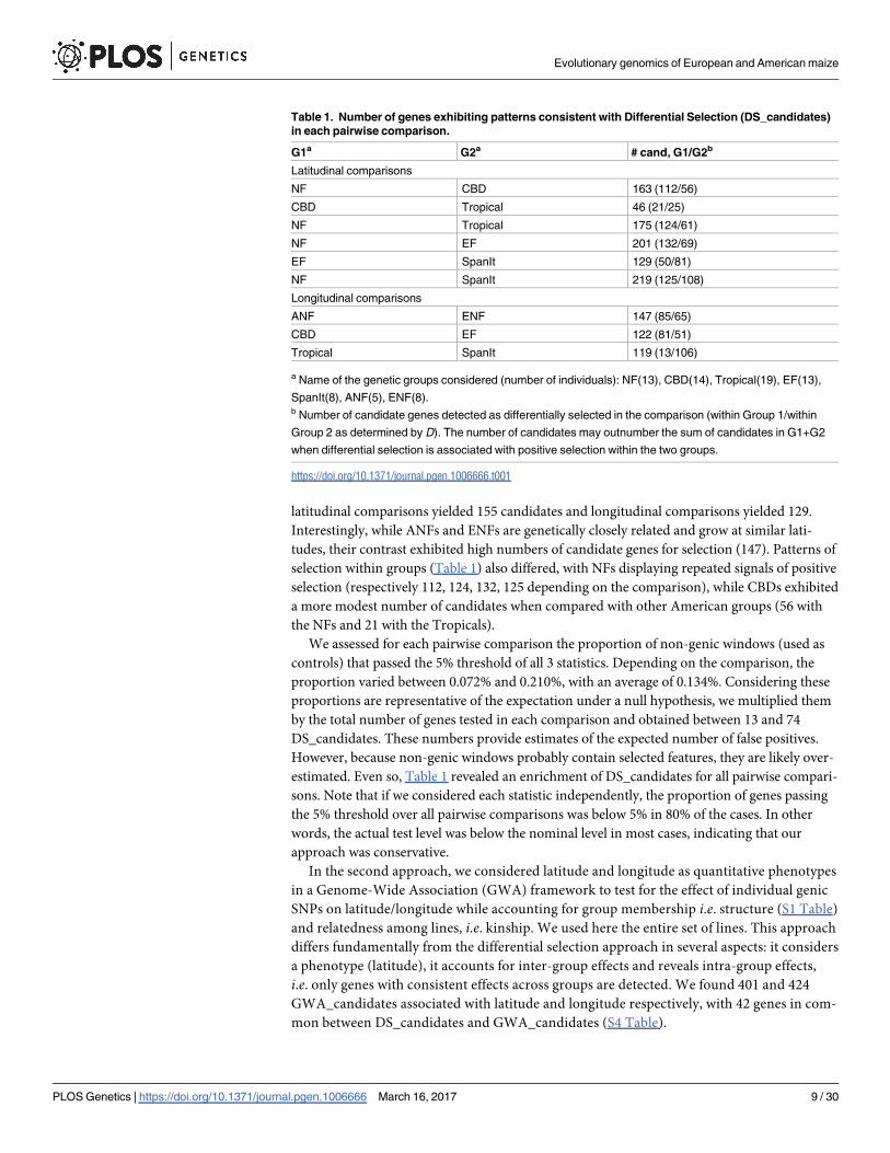
latitudinal comparisons yielded 155 candidates and longitudinal comparisons yielded 129.

Interestingly, while ANFs and ENFs are genetically closely related and grow at similar lati-

tudes, their contrast exhibited high numbers of candidate genes for selection (147). Patterns of

selection within groups (Table 1) also differed, with NFs displaying repeated signals of positive

selection (respectively 112, 124, 132, 125 depending on the comparison), while CBDs exhibited

a more modest number of candidates when compared with other American groups (56 with

the NFs and 21 with the Tropicals).

We assessed for each pairwise comparison the proportion of non-genic windows (used as

controls) that passed the 5% threshold of all 3 statistics. Depending on the comparison, the

proportion varied between 0.072% and 0.210%, with an average of 0.134%. Considering these

proportions are representative of the expectation under a null hypothesis, we multiplied them

by the total number of genes tested in each comparison and obtained between 13 and 74

DS_candidates. These numbers provide estimates of the expected number of false positives.

However, because non-genic windows probably contain selected features, they are likely over-

estimated. Even so, Table 1 revealed an enrichment of DS_candidates for all pairwise compari-

sons. Note that if we considered each statistic independently, the proportion of genes passing

the 5% threshold over all pairwise comparisons was below 5% in 80% of the cases. In other

words, the actual test level was below the nominal level in most cases, indicating that our

approach was conservative.

In the second approach, we considered latitude and longitude as quantitative phenotypes

in a Genome-Wide Association (GWA) framework to test for the effect of individual genic

SNPs on latitude/longitude while accounting for group membership i.e. structure (S1 Table)

and relatedness among lines, i.e. kinship. We used here the entire set of lines. This approach

differs fundamentally from the differential selection approach in several aspects: it considers

a phenotype (latitude), it accounts for inter-group effects and reveals intra-group effects,

i.e. only genes with consistent effects across groups are detected. We found 401 and 424

GWA_candidates associated with latitude and longitude respectively, with 42 genes in com-

mon between DS_candidates and GWA_candidates (S4 Table).

Table 1. Number of genes exhibiting patterns consistent with Differential Selection (DS_candidates)

in each pairwise comparison.

G1a G2a # cand, G1/G2b

Latitudinal comparisons

NF CBD 163 (112/56)

CBD Tropical 46 (21/25)

NF Tropical 175 (124/61)

NF EF 201 (132/69)

EF SpanIt 129 (50/81)

NF SpanIt 219 (125/108)

Longitudinal comparisons

ANF ENF 147 (85/65)

CBD EF 122 (81/51)

Tropical SpanIt 119 (13/106)

a Name of the genetic groups considered (number of individuals): NF(13), CBD(14), Tropical(19), EF(13),

SpanIt(8), ANF(5), ENF(8).b Number of candidate genes detected as differentially selected in the comparison (within Group 1/within

Group 2 as determined by D). The number of candidates may outnumber the sum of candidates in G1+G2

when differential selection is associated with positive selection within the two groups.

https://doi.org/10.1371/journal.pgen.1006666.t001



https://doi.org/10.1371/journal.pgen.1006666.t001


From candidates to gene ontology to selection along gene networks

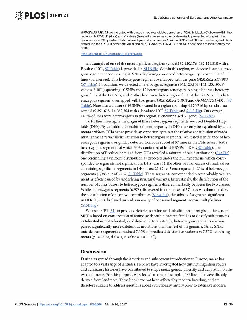
An example of a DS_candidate is illustrated in Fig 4. Patterns at SU1 revealed reduced diver-

sity in the CBDs as compared with the NFs (Fig 4A), and XP-CLR values deviating from

the genome-wide estimates (Fig 4C, S3 Table). Consistently, one main haplotype segregated

around SU1 within CBDs and to a lesser extent within Tropicals, with an overall elevated

level of LD within this region (Fig 4B). Selection within CBDs was further confirmed by sig-

nificantly negative D values (Fig 4C, S3 Table). Note also selective footprints in the region

surrounding the nearby domestication gene TGA1, as illustrated by elevated LD with the

segregation of two major haplotypes (Fig 4B).

Association between latitude and allele frequency was found at GRMZM2G095955 (GWA_

candidate, S4 Table), a gene located in the vicinity of maize floral activator, ZCN8 [29]. Pat-

terns in the ZCN8 region revealed a haplotype common to all temperate material and the seg-

regation of this “temperate” haplotype with a “tropical” haplotype within Tropicals and to a

lesser extent within CBDs (S9 Fig).

Along with previously characterized genes, we also revealed new candidates such as ZCN5,

which is also known as PEBP5. This gene harbored strong evidence of selection both within

the Tropicals (S10C Fig) and within the European Flints when compared with the NFs with

corresponding significant negative D values (S3 Table). A specific haplotype for these groups

differed markedly from the most common NF haplotype (S10B Fig). Interestingly, both haplo-

types segregated at intermediate frequency within the CBDs (S10B Fig), as denoted by a signif-

icant positive D (S3 Table, S10C Fig).

Considering candidate genes detected among all pairwise comparisons in both DS_ and

GWA_ approaches, we found significant enrichment in 19 MapMan ontologies (S5 Table).

We further grouped MapMan ontologies into 23 main categories, and found enrichment in 2

out of the 23 main categories: carbohydrate metabolism, proteins (S5 Table).

We also tested for a global enrichment of differential selection signals (using Fst) at the

gene network level rather than at the individual gene level, following a method proposed by

[30]. In this purpose, we used 294 maize gene networks described in the MaizeCyc database.

We found 62 significant pairwise comparisons at α<1%, corresponding to 44 gene networks.

Because some gene networks had more than 50% of genes in common, we grouped genes into

25 network clusters (S6 Table). Among network clusters with a potential role in adaptation,

we found signs of selection on the abscissic acid (ABA) biosynthesis network (Network Cluster

#2, S6 Table), the putrescine pathway (Network Cluster #9, S6 Table), the β-caryophyllene

biosynthesis pathway (Network Cluster #11, S6 Table), the cis- and trans- zeatin biosynthesis

pathways (Network Cluster #18, S6 Table).

Genome-wide distribution of residual heterozygosity

We developed a segmentation method to detect regions with patterns of heterozygosity that

deviate from genome-wide expectations, i.e. heterozygous segments. We applied our method

to the subset of 57 first-cycle inbred and SSD lines. Deviations were detected either because

heterozygosity extended over an unexpectedly high number of adjacent sites (in a single or

multiple lines) or because heterozygosity was unexpectedly conserved across lines (at a single

or multiple sites). We retained 17,959 segments genome-wide, each encompassing at least 5

SNPs. Among these, 6,978 exhibited significantly elevated heterozygosity relative to that of the

entire genome (0.41%) as determined by an exact Bernoulli test procedure followed by an FDR

control at a nominal level of 5% (S7 Table). Heterozygous segments encompassed/overlapped

with 4,354 annotated genes (S7 Table). They covered a total of 166,892,128 bases. No particular

distribution pattern was observed at the chromosome level (S11A Fig).




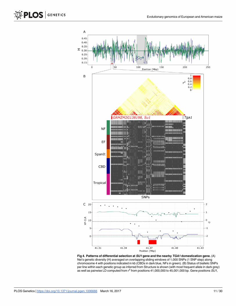
Fig 4. Patterns of differential selection at SU1 gene and the nearby TGA1 domestication gene. (A)

Nei’s genetic diversity (H) averaged on overlapping sliding windows of 1,000 SNPs (1 SNP step) along

chromosome 4 with positions indicated in kb (CBDs in dark blue, NFs in green). (B) Status of biallelic SNPs

per line within each genetic group as inferred from Structure is shown (with most frequent allele in dark grey)

as well as pairwise LD computed from r2 from positions 41,000,000 to 45,001,000 bp. Gene positions SU1,




An example of one of the most significant regions (chr. 6,162,120,176–162,124,810 with a

P-value<10−6, S7 Table) is provided in S11B Fig. Within this region, we detected one heterozy-

gous segment encompassing 20 SNPs displaying conserved heterozygosity in over 33% of

lines (on average). This heterozygous segment overlapped with the gene GRMZM2G174990(S7 Table). In addition, we detected a heterozygous segment (162,126,864–162,133,490, P-

value = 6.10−6) spanning 10 SNPs and 12 heterozygous genotypes. A single line was heterozy-

gous for 5 of the 12 SNPs, and 7 other lines were heterozygous for 1 of the 12 SNPs. This het-

erozygous segment overlapped with two genes, GRMZM2G174949 and GRMZM2G174971 (S7

Table). Note also a cluster of 19 SNPs located in a region spanning 4,170,746 bp on chromo-

some 6 (9,891,618–14,062,364 with a P-value<10−6, S7 Table and S11A Fig). On average

14.9% of lines were heterozygous in this region. It encompassed 37 genes (S7 Table).

To further investigate the origin of these heterozygous segments, we used Doubled Hap-

loids (DHs). By definition, detection of heterozygosity in DHs may only be explained by align-

ments artifacts. DHs hence provide an opportunity to test the relative contribution of reads

misalignment versus allelic variation to heterozygous segments. We tested significance of het-

erozygous segments originally detected from our subset of 57 lines in the DHs subset (6,978

heterozygous segments of which 5,069 contained at least 5 SNPs in DHs, S7 Table). The

distribution of P-values obtained from DHs revealed a mixture of two distributions (S12 Fig):

one resembling a uniform distribution as expected under the null hypothesis, which corre-

sponded to segments not significant in DHs (class 1); the other with an excess of small values,

containing significant segments in DHs (class 2). Class 2 encompassed ~21% of heterozygous

segments (1,088 out of 5,069, S7 Table). These segments corresponded most probably to align-

ment artefacts caused by underlying structural variants. Interestingly, the distribution of the

number of contributors to heterozygous segments differed markedly between the two classes.

While heterozygous segments (6,978) discovered in our subset of 57 lines was dominated by

the contribution of one or two contributors (S13A Fig), the subset of segments significant

in DHs (1,088) displayed instead a majority of conserved segments across multiple lines

(S13B Fig).

We used SIFT [31] to predict deleterious amino acid substitutions throughout the genome.

SIFT is based on conservation of amino acids within protein families to classify substitutions

as tolerated or not tolerated, i.e. deleterious. Interestingly, heterozygous segments encom-

passed significantly more deleterious mutations than the rest of the genome. Genic SNPs

outside those segments contained 7.07% of predicted deleterious variants vs 7.57% within seg-

ments (χ2 = 23.78, d.f. = 1, P-value = 1.07 10−6).

Discussion

During its spread through the Americas and subsequent introduction to Europe, maize has

adapted to a vast range of latitudes. Here we have investigated how distinct migration routes

and admixture histories have contributed to shape maize genetic diversity and adaptation on the

two continents. For this purpose, we selected an original sample of 67 lines that were directly

derived from landraces. These lines have not been affected by modern breeding, and are

therefore suitable to address questions about evolutionary history prior to extensive modern

GRMZM2G138198 are indicated with boxes in red (candidate genes) and TGA1 in black. (C) Zoom within the

region with XP-CLR (dots) and D values (lines with the same color code as in A) presented along with the

genome-wide 5% quantile (dark blue and green dotted line for D within CBDs and NFs respectively, and black

dotted line for XP-CLR between CBDs and NFs). GRMZM2G138198 and SU1 positions are indicated by red

boxes.






breeding. We have generated whole genome sequencing to produce a dataset of SNPs with

reduced ascertainment bias and allele frequencies that include low frequency variants (S4 Fig).

Maize is characterized by high nucleotide diversity (10–20 times greater than humans [32]),

a vast amount of structural variation [33], and extended paralogy [34]. Our methodology has

accounted for those specificities and allowed accurate detection of homozygous SNPs despite

the complexity of the maize genome. Our estimated miscall rate of 0.036% is about 8 times

lower than that estimated from 5x whole genome sequencing data (0.31%, [20]). We geno-

typed over 22 million SNPs that covered 87% of annotated genes, providing the largest whole

genome sequencing effort to date of the maize European germplasm.

Characterizing regions with unexpected patterns of heterozygosity

Heterozygotes are much more challenging to call than homozygotes particularly with coverage

<20x [35]. Consistently, we found a much higher rate of false positives (34%) for heterozy-

gotes. This rate still compares advantageously to previous estimates from 103 lines, which had

a false positive rate of nearly 75% [20]. A small proportion of heterozygotes miscalling may be

explained by genotyping errors in the data generated by the MaizeSNP50 array. We indeed

found examples of array-called heterozygous SNPs in our sample of 3 doubled-haploids

(0.16% of genotypes on average).

Although heterozygotes calling in our HTS dataset was error prone, we have postulated that

extended segments of heterozygosity (along a region or among lines) provide evidence for

either mapping artifacts caused by underlying structural variants (duplications) or regions that

are resistant to homozygosity. Selection against allele combinations that are highly deleterious

when homozygous may indeed help overcoming inbreeding depression. Previous studies have

proposed that elevated rate of heterozygosity in low-recombining pericentromeric regions of

recombinant inbred lines is a consequence of inefficient purging of deleterious alleles [36,37].

In contrast, we have observed no specific patterns of heterozygosity along the chromosomes

(S8 Fig).

Because deleterious alleles segregate at low frequencies in the maize genome, they are diffi-

cult to use in association mapping frameworks that combine genotypes and phenotypic mea-

sures of inbreeding depression [38]. The power of our segmentation approach is to rely on

repeated evidence, either among lines or regions, to discover regions of unexpectedly high het-

erozygosity. Using a subset of 57 first-cycle inbreds and SSD lines (out of 67), we identified

6,978 segments of unexpectedly high heterozygosity rate. Together, these heterozygous seg-

ments represent 8.8% of all base pairs analyzed. A substantial proportion of heterozygous seg-

ments (~21%) also displayed an elevated rate of heterozygosity in our subset of 10 doubled

haploids, consistent with alignment artefacts caused by underlying structural variants. On chro-

mosome 6, for example, we found a segment of extended heterozygosity bearing 37 genes

(S11A Fig), 6 of which are reported as part of the highest read depth variants in maize [20], sig-

naling a structural variant recently confirmed by PCR assays in a collection of lines [39]. But the

majority of our heterozygous segments were not detected in doubled haploids and may there-

fore point to inbreeding depression candidates. While the difference is small, we actually found

significantly more deleterious variants in heterozygous segments (7.57%) than in the rest of the

genome (7.07%). Altogether, our results suggest that selection against inbreeding depression

has played a role in the maintenance of residual heterozygosity in our sample of maize lines.

American sources and footprints of European introductions

In the Americas, two historical major expansions northwards and southwards from Mexico

have been documented [13] (Fig 1). The northwards expansion through southwestern US to




the northern US and Canada gave rise to the Northern Flints [40,41]. Introduced around 500

BC, Northern Flints gradually became the main crop in eastern North America [42]. Southern

Dents appeared 2000 yrs later and likely derived from southeastern US introductions with

influence of Caribbean flints [43,44]. Corn Belt Dents (CBDs), that are adapted to the Mid-

western US climate, emerged about 200 years ago from crosses between southern Dents and

Northern Flints [43]. Our data confirmed their admixed origin (S7A Fig) but also pointed to a

greater contribution of Southern material. Interestingly CBDs in the Treemix analysis (Fig 2)

appeared to share a close ancestor with the Caribbean rather than with Mexican material, per-

haps mirroring the Caribbean contribution to the Southern Dents [43].

We have combined evidence from inferred genetic proximities and admixture events

revealed by Treemix as well as historical records to propose a model of maize migration in

Europe (Fig 1). Our data are consistent with two major introductions in Europe. First genetic

proximity between European and American Northern Flints (ANFs and ENFs) indicate that

the latter derived from the former (Fig 2). Second, the Spanish materials appear to share a

common ancestor with the South American material (Fig 2). The latter observation questions

the Caribbean origin of Spanish maize. Because there is clear evidence that Columbus

imported maize from Cuba to Spain by 1493 [45], it is possible that our limited sample did not

capture the source of the Spanish material but rather the South American origin of the Carib-

bean material subsequently introduced in Southern Europe.

Regarding a putative third independent introduction of the Italian material from Argentina

[16], our results were more consistent with the emergence of Italian lines from an admixture

between Spanish and European Flints (Fig 2). Letters actually attest to the donation of maize

from Spain to the Vatican in Rome after the second voyage of Columbus as early as 1494 [46].

Finally, we have substantiated—with a much larger dataset than [15,16]–the admixed origin of

the European Flints (EFs) from two contributors, the ENFs and the Tropicals.

Altogether our results show that while genetic diversity is significantly lower in Europe

than in America (Fig 3A & 3C), European introductions left only modest footprints on the dis-

tribution of allele frequencies (Fig 3B). We found evidence for two independent introductions

to Europe and propose that adaptation to mid-latitudes both in the US (CBDs) and Europe

(EFs and Italians) has depended on admixture.

Screening for genic targets of selection along latitude and longitude

Our sample encompassed 5 genetic groups (Fig 1B and S5B Fig) distributed over a broad

range of latitudes along two longitudinal axes (the two continents). Both latitude and longitude

are primary determinants of climate variation. However, because locations at the same latitude

share identical day-length and seasonalities and often similar climates [2], we expect latitudinal

contrasts to reveal more adaptations than longitudinal contrasts. Consistently, among Differ-

entially Selected candidates (DS_candidates) we have observed on average more candidates

in latitudinal contrasts (155 genes) than in longitudinal contrasts (129 genes). However, the

opposite trend was observed in the GWA analysis (401 versus 424), perhaps highlighting the

role of other adaptive forces such as habitats and biotic components. The number of DS_can-

didates detected for the Northern Flints (>112 in all comparisons, Table 1) outnumbered

those detected for the Tropicals (<61 in all comparisons), signaling more pervasive adaptation

outside latitudes where maize originated.

In total, we retrieved 968 DS_candidates. In order to control the rate of false positives, we

based our DS_candidates identification on genome-wide extreme values for three metrics

(CLR test, Fst, D) that detect different hallmarks and time scales of selection [47]. While our

approach was conservative, the comparison with the recent work of Unterseer and colleagues




[21] that employed a similar methodology to detect DS_candidates revealed a greater number

of common DS_candidate genes between the two studies (93, S3 Table) than expected by

chance (P-value<2.10−3). Unterseer and colleagues [21] have contrasted Flint elite lines—

grouping EFs and NFs from Europe—to Dent elite lines developed in Europe and the US, and

accordingly most common DS_candidate genes (59 among 93) originated from our Flints and

Dents comparisons (EFs/CBDs and NFs/CBDs). While significant, the overlap between the

two studies was overall limited: first because the two studies differ in the time scale analyzed,

recent breeding (elite lines were included in [21]) versus more ancient adaptive events repre-

sented by the first-cycle inbred lines in our study; second because we included tropical materi-

als, thereby expanding our ability to find loci involved in the first steps of adaptation towards

northern latitudes. More generally, although false positives may contribute to differences

between studies, our results are consistent with the recruitment of distinct genetic mechanisms

in different genetic groups.

Because polygenic adaptation may involve a collection of mutations with small effects,

which collectively have a large effect on a given pathway, we adapted a gene-set enrichment

test [30] to uncover genome-wide signals of differential selection along 294 gene networks.

We found evidence for differential selection at 25 candidate gene network clusters (S5 Table).

Overall, common signals of selection detected at individual genes and along gene networks

were scarce. In fact, while our networks together encompassed 627 genes, only 16 genes that

were detected as candidates by the gene-by-gene approach also belonged to selected networks

(S3 Table). This result may illustrate potential complementarity of these two approaches, with

the former detecting genes with potential strong allelic effect, while the latter aims at detecting

polygenic adaptation emerging from selection of a multitude of alleles with small effects.

Multifarious adaptation of maize

While a small fraction of our candidates has been functionally characterized in maize (S3 and

S4 Tables), we can point to a number of interesting examples. For instance, we found a signifi-

cant association between a polymorphism located in the vicinity of ZCN8 and latitudinal varia-

tion (S9 Fig). ZCN8 is the main floral activator of maize [29], and it is strongly associated with

flowering time variation [48]. Here, patterns at ZCN8were consistent with segregation of two

haplotypes in the Tropicals, and elimination of the late flowering haplotype from northern lati-

tudes (late flowering haplotype displayed in light grey, S9 Fig). With a single exception, the late

flowering haplotype was also counter-selected within CBDs and within EFs after admixture

events in North America and Europe respectively. Interestingly, we also found signals of posi-

tive selection ZCN5 (also known as zen1 and pebp5), a gene from the same family as ZCN8.

Here the “tropical” haplotype present in Tropicals strongly differed from the major “NF”

haplotype (S10 Fig). In contrast to CBDs that exhibited the two haplotypes at intermediate

frequency, the pattern in EFs was consistent with strong positive selection of the “tropical”

haplotype in this group (S10 Fig). ZCN5 is expressed in developing ears and tassels after floral

transition in maize but its function remains undetermined [49]. While it is beyond the scope

of our paper to perform functional validations, a recent study has reported an association

between polymorphisms at ZCN5 and flowering time variation [50].

Besides flowering, which is an obvious target of selection, we have also uncovered an

important role for abiotic stress tolerance in maize adaptation. We have found significant

enrichment for the tetrapyrrole synthesis category both in our gene-by-gene (S5 Table) and

network approaches (S6 Table), as well as evidence of selection along the ABA synthesis gene

network in ANFs/ENFs comparisons (S6 Table). One of our candidates, the ZmASR2 gene

(Abscisic acid-, Stress-, and Ripening-induced protein 2, GRMZM5G854138, S3 Table) actually




displays increase in expression at the transcript and protein level under water deficit condi-

tions [51]. Both ABA and tetrapyrroles entail drought tolerance via independent stimuli, cellu-

lar changes—loss of turgor—for the former, and ROS-mediated stress signaling for the latter

[52]. Cold tolerance also contributed to maize spread as manifested by selection along the

putrescine pathway (S6 Table)—and the largely redundant arginine degradation III arginine

decarboxylase-agmatinase pathway—in multiple pairwise comparisons. The putrescine path-

way is part of the polyamine metabolism activated in response to various abiotic stresses [53].

In Arabidopsis thaliana, putrescine controls ABA level in response to low temperature, thereby

contributing to cold acclimation [54]. Along the same lines, we have revealed strong evidence

of selection along cis- and trans-zeatin pathways in pairwise comparisons involving NFs vseither Tropicals or SpanIt (S6 Table). The zeatin biosynthesis pathways mediate responses to

biotic and abiotic environmental interactions [55]. They are considered essential cytokinins

and in conjunction with ABA are involved in various stress responses including cold, drought,

and osmotic stresses [56].

Biotic factors are equally important contributors to maize adaptation and spread. We have

found footprints of selection along the β-caryophyllene biosynthesis network in comparisons

involving EFs versus Tropicals or CBDs (S6 Table). β-caryophyllene is a secondary metabolite

that serves as foraging cues for natural enemies of herbivores [57]. The pathway includes the

TPS23 gene (GRMZM2G127336) responsible for the synthesis of a volatile sesquiterpene that

attract natural enemies of herbivores upon release [58]. Interestingly, evidence from 24 North

American lines suggest that the majority (22 out of 24) have lost the capacity of synthetizing

this component [59], while the gene is actively transcribed in European material. Consistent

with these observations, our results revealed selection within EFs at GRMZM2G127336 (S3

Table). Likewise, selection at 6 genes from theWRKY family (S3 and S4 Tables) support the

adaptive contribution of DNA binding transcription factors that regulate plant defense in

response to various infections such as Trichoderma root colonization [59] and fungal patho-

gens [60]. For instance, expression of the putative Arabidopsis thaliana ortholog ofWRKY41(S3 Table), AtWRKY46, is strongly induced by pathogen effectors, and therefore likely

involved in the transcriptional reprogramming that initiate effector-trigger immunity [61].

In addition to phenology, abiotic and biotic stress responses, patterns at the SU1 gene

(GRMZM2G138060, S3 Table and Fig 4)—that encodes a starch debranching enzyme—uncov-

ered differential selection on kernel phenotypes between NFs and CBDs [62]. In conjunction

with other starch biosynthesic components [63], SU1 contributes to the structure of amylopec-

tin as well as the ratio of amylose over amylopectin, which affects gelatinization properties

and texture [64]. SU1 was targeted by selection during domestication [64]. Moreover, previous

work has demonstrated gradual allelic selection at SU1 from teosintes to early maize and to

modern varieties [65]. The region bearing SU1 and TGA1, one of the key domestication gene

conferring the naked grain maize phenotype [66], displays strong linkage disequilibrium (Fig

4) consistently with previous observations [48]. Note that TGA1 displayed no clear footprints

of species-wide past selection despite the indisputable effect of a single amino acid substitution

in the acquisition of the domesticated phenotype. Close interactions between TGA1 and the

nearby NOT1 gene contribute to numerous pleiotropic effects and traits—including branch-

ing, kernel shape and size [67]. The complexity of effects and their interactions may produce a

complex pattern of haplotypes.

Conclusion

We scored over 22 million SNPs in American and European maize germplasm with high accu-

racy. This dataset helped refine a scenario consisting of two major introductions of maize to




Europe. The range of latitudes in Europe represents a restricted subset of latitudes in the North

America. We found that independent introduction sources and subsequent admixtures are

keys to the spread of maize through Europe, mirroring the emergence of the admixed Corn

Belt Dents in the US. This repeated pattern of admixture with newly introduced groups has

contributed to adaptive innovations, paralleling recent findings in humans. Future work

should help unravel the genome-wide specific contribution of parental groups to these

admixed groups.

Materials and methods

Sampling and sequencing

We directed our sampling towards first-cycle inbred lines directly derived from landraces after

a few generations of selfing. We established a list of all available first-cycle inbreds and gath-

ered historical information to establish the name and geographic location of the corresponding

landraces. Our sample included 48 of these lines. However, for the Mexican, Caribbean and

South American lines, only a very small set of first cycle inbreds was available. We therefore

used 9 Single Seed Descents (SSDs) and 10 Doubled Haploids (DHs) recently derived from

Tropical landraces instead. Note that 8 of these SSDs were previously sequenced in [20]. The

geographical locations of landraces from which the lines were derived is shown in Fig 1.

Our final sample encompassed 67 lines including 14 Corn Belt Dents (CBDs), 5 American

Northern Flints (ANFs), 8 European Northern Flints (ENFs), 13 European Flints (EFs), 3

Spanish (Span), 5 Italians (It), 7 South Americans (2 and 5 respectively from the Northern and

the Southern part), 7 Mexicans (5 lowlands and 2 highlands below/above 1500 meters) and 5

Caribbeans. We referred to Tropicals when combining South Americans, Mexicans and Carib-

beans (19 Lines). Sample information with name, origin, provider, and status is available in S1

Table.

Genomic DNAs of all lines were extracted from fresh leaf tissue of a single plant using the

Macherey-Nagel MaxiKit and sent to Integragen (Evry, France) for library construction and

sequencing. Sheared total genomic DNA was used to generate Illumina paired-end libraries

(500 bp insert size). Each library was paired-end sequenced (2 x 101 bp) with a target sequenc-

ing depth of 15x. Sequencing data volume for each line is detailed in S1 Table. DNA-sequenc-

ing reads from all lines were deposited in the European Nucleotide Archive (ENA) under the

study accession number PRJEB14212.

Mapping and SNP calling

All lines were aligned to the B73 v2. reference genome by combining Bowtie2 [68] and Stampy

[69]. First Bowtie2 was used with default parameters, using a>98% identity threshold between

each sample and the reference genome (parameter - -score-min L,0,-0.12). In a second step,

unmapped reads were used for mapping with Stampy (default parameters), which is a slower

but more accurate aligner for insertion-deletion types of polymorphisms [69]. From SAM for-

mat outputs, we sorted and filtered out duplicates using Samtools V1.1 [70]. A total of 2,654

Gb of Illumina reads from the 67 samples were used to extract mpileup format with Samtools

using properly mapped pairs only. We used mpileup raw counts to estimate genome coverage

and read depth of each line. We considered as covered any base with at least 4 reads.

We performed genotype calling for each SNP with Varscan using the following parameters:

Phred score above Q20, minimum coverage of 6 reads, α = 5%. For each sample, Varscan pro-

vides the number of reads that support variants at a given SNP. We utilized this information to

define genotypes by performing a Likelihood Ratio Test (LRT) with one degree of freedom fol-

lowing [71] with slight modifications. Let n1 and n2 be the counts of most frequent and second




most frequent nucleotide variants, we computed the likelihoods of a homozygote (genotype

1/1) or a heterozygote (1/2) as follows: L (1/1) ~ B(n1+n2,ε) and L (1/2) ~ B (n1+n2, 0.5), with

the error rate ε = 0.01. If LRT was significant at α = 5%, we assigned the most likely genotype

at the SNP.

Customized filters and genotyping accuracy

After individual genotype calling, we considered the genotype information across samples to

apply filters and improve genotype-calling accuracy. We retained only SNPs with two variants

(biallelic). Our filters aimed at increasing proper SNP identification, and eliminating false het-

erozygosity created by misalignment of duplicated (paralogous) regions. We employed four

criteria described below: multiple mapping, sequencing-depth variation, error rate, heterozy-

gosity rate.

Multiple mapping. To avoid false genotype calling arising from genome redundancy, we

retained genotypes (lines) for which the percentage of reads mapping to unique genomic posi-

tions was >90%. For reads aligned with Stampy, we used an alignment score>11 to define

uniquely-mapped reads. We discarded positions that presented both ambiguous (with regards

to multiple-mapped reads) and heterozygous genotypes.

Sequencing-depth variation. We eliminated genotyping information for all lines with a

low sequencing-depth (<6) at a given position. In addition, we discarded positions with an

average sequencing-depth > 28 across samples (28 represents the 99% average upper bound of

the coverage). Such an elevated depth likely corresponds to missing portions in the reference

genome and/or duplicated regions in our samples.

Error rate. For each genotype, we evaluated the error rate as the number of reads that dif-

fered from the called genotype, as given by the LRT (see above). We dropped positions for

which (1) the probability of observing the number of error counts or more is above α = 5%

given that B (n1+n2, ε), with ε = 0.01; (2) the distribution of the error counts among samples

significantly differs from a Poisson distribution of parameter the average error count at the

position (Kolmogorov-Smirnov test, α = 5%).

Heterozygosity rate. We eliminated heterozygous genotypes located in close vicinity

(< 500 bp) to heterozygous insertion-deletions (indels). Local alignments are indeed known

to be less accurate in regions encompassing such indels. When a heterozygote was detected

among the 67 Lines, we retained only positions for which at least one homozygote of each vari-

ant was detected in other lines.

We extracted all positions that passed our stringent filters and determined the distribution

of missing genotyping information across SNPs as well as the percentage of missing data per

line. We annotated SNPs and classified them in two categories: within and outside genes.

SNPs within genes were further subdivided into belonging to 5’UTR, 3’ UTR, exonic and

intronic regions. Throughout the text, non-genic SNPs are defined as SNPs located >50kb

away from annotated genes, and genic SNPs are defined as SNPs located within genes and

10kb on both sides of the genes.

Genotype calling accuracy

To test the accuracy of our genotype calling we employed several approaches. First, we com-

pared the rate of heterozygosity per line before and after applying our customized filters. We

computed the per-line heterozygosity as the number of heterozygous sites divided by the num-

ber of heterozygous and homozygous sites for the alternative allele (allele differing from the

reference). By considering alternative homozygotes only, this estimate compares each line to

the reference independently from the level of diversity in the rest of the sample.




Second, we used 2 sets of high-confidence genes defined by [27] as “retained homoeologs”

and “lost homoeologs”. The former encompasses genes with paralogs within the B73 genome,

while the latter corresponds to single genes in B73 (with no paralogous copy). We expect no

significant difference in the heterozygosity rate between those two sets of genes if our filters

were efficient to discern true heterozygotes from homozygotes for different alleles at two dupli-

cated loci. We retained genes with less than 30% of missing data—for a total of 2,788 genes

with paralogs and 3,949 single genes—and computed the rate of heterozygosity per gene across

our sample of 67 lines. We tested difference in the rate of heterozygosity between the two sets

of genes using a bilateral Kolmogorov-Smirnov test (α = 5%).

Third, we extracted positions of the Illumina Maize SNP50k array from our HTS data to

compare genotypes. For 42 lines, array genotyping was already available [72] but the DNAs

used for genotyping came from different seed lots than the ones we used for HTS. Because

first-cycle inbred lines exhibit residual heterozygosity, a substantial amount of heterozygous

genotypes may differ between and within seed lots derived from the same line. We therefore

also generated for another 20 lines new MaizeSNP50k genotyping from the exact same DNAs

that served to produce the HTS data (S1 Table). We used Genome Studio (Illumina, v1) to call

genotypes by applying the manually curated clustering of [73]. We first restricted our analysis

to homozygotes both in Maize SNP50k array and HTS data. We calculated the error rate of

genotype calling in our HTS data as the ratio of the number of discrepancies between the 2

datasets divided by the total number of genotypes evaluated, and considered either all 62

lines or the subset of 20 lines. Second, we used the subset of 20 lines to calculate errors rates for

heterozygotes. We determined the false positive rate of HTS genotyping as the number of het-

erozygotes declared as homozygotes on the MaizeSNP50k divided by the number of heterozy-

gotes in our HTS data. Conversely, we estimated the false negative rate as the number of

heterozygotes found in the MaizeSNP50k but declared as homozygotes in our HTS data.

Patterns of heterozygosity along chromosomes

We aimed at identifying regions with heterozygosity patterns deviating from the genome wide

expectation across our sample of first-cycle inbreds and Single Seed Descent (SSD) lines (57).

In order to do so, we employed a segmentation method on positions with MAF>5%. We con-

sidered the following statistical model. Let Xij stand for the heterozygous status of line i at posi-

tion j, with Xij = 1 if the line is heterozygous, 0 otherwise. On a given chromosome, positions

were assumed to be spread into K contiguous regions, each of these regions being character-

ized by a specific Heterozygosity Rate (HR), i.e. Xij~B(pk) if position j belongs to region k,

where B(.) is the Bernoulli distribution and pk is theHR in region k. The goal of the statistical

analysis was to identify regions with associatedHR pk significantly higher than the genome

wide HR. To this aim, a 2-step statistical analysis was performed.

In step 1 we applied a breakpoint detection procedure to jointly segment the heterozygous

profiles and identify regions with homogeneous HR. When the number of regions K is known,

the breakpoint detection problem boils down to finding the optimal splitting of the chromo-

some into K regions along with their associated HR{p1,. . .,pK}. A combination (splitting, HR{p1,. . .,pK}) is optimal if it achieves the best fit to the data, the fitting being measured through

the likelihood. Identification of the combination (splitting, HR {p1,. . .,pK}) optimizing the like-

lihood was achieved through dynamic programming [74,75]. Since in practice the number of

regions is unknown, we considered different values for K, ranging from 1 to 20,000. We fur-

ther selected the optimal value K� using the model selection criterion proposed in [76].

In step 2, we applied a test procedure to identify regions with aHR significantly higher

than the genome wideHR, noted pg. For a given region, the procedure consisted in testing




H0 {pK = pg} vs H1 {pK> pg} using an exact Bernoulli test procedure. To control for multiple

testing, a Benjamini Hochberg procedure [77] was performed at a nominal level of 5%. The

true genome wideHR being unknown, we considered pobs (0.41%) as the best estimate of pg,where pobs is the genome wide averagedHR computed on the first-cycle inbred lines and SSDs

(57). Note that pobs was calculated as the number of heterozygotes divided by the number of

heterozygotes and homozygotes. The previously described 2 steps procedure was applied to 57

lines (first-cycle inbreds and SSD lines).

For better visualization, we first merged independently significant (resp. non-significant)

adjacent segments; second we removed segments containing a single SNP; and third we

repeated the merging. In the end, we retained segments containing at least 5 SNPs. In the fol-

lowing we denoted segments displaying unexpected patterns of heterozygosity as heterozygous

segments.

For heterozygous segments, we calculated the rate of heterozygosity in our subset of 10

HDs. We also determined the corresponding P-values using the test procedure described

above.

We next asked whether heterozygous segments were enriched for deleterious mutations. To

this purpose, we extracted genome wide genic SNPs and used SIFT4G_Annotator_v2.3 with

the corresponding maize database [31] to identify both tolerated and deleterious variants. We

tested for enrichment of deleterious variants within heterozygous segments compared with the

rest of the genome using a χ2 test.

Because heterozygotes represented a small proportion of all genotypes, in all subsequent

analyzes we considered heterozygotes as missing data and relied on a haploid model.

Site frequency spectra and summary statistics

To evaluate the distributions of allele frequencies in our samples, we generated folded Site Fre-

quency Spectra (SFS) using the DaDi (Diffusion approximation for Demographic inference)

python library [78]. When constructing spectra, we projected down the sample size to account

for missing data and differences in sample size. We generated folded SFS for (1) the entire

sample of lines restricted to positions of the Maize SNP50k array, and (2) the entire sample

(SFS projected down to 60 samples). Additionally, we retrieved all SNP positions available

from Tripsacum dactyloidesHTS data [20] to infer the ancestral versus derived status of our

SNPs, and built an unfolded SFS considering the entire set of 67 Lines (projected down to 60

as above).

In order to further test the impact of introduction bottlenecks, we generated SFS on Ameri-

can and European lines (projected down to 29 samples) using non-genic SNPs. We compared

our observed American SFS to the predicted “neutral” SFS obtained from a demographic

model recently established by [28] for American landraces. This model incorporates a domes-

tication bottleneck occurring 15,000 generations as well as a population expansion, and

accounts for gene flow between wild and cultivated forms. We simulated sequences of 38 sam-

ples with MS [79] using the parameters indicated in Fig. 2 of [28] with an instantaneous expan-

sion. We further established the corresponding SFS downsized to 29 samples. For non-genic

SNPs, we also computed for American and European lines, genome-wide per-bp summary sta-

tistics with corrections for missing data [80]: π[81], Watterson’s θ [82], and Tajima’s D (D)

[83]. In order to assess the significance of the difference in the amount of diversity between

American and European samples, we estimated π on non-overlapping non-genic windows of

10kb along the genome (with less than 50% missing positions) and applied a pairwise Wil-

coxon signed-rank test. Genetic diversity along chromosomes for the American and European

samples as measured by π was computed on 50kb overlapping sliding windows with a step of




10kb. We used local linear polynomial fit for smoothing with lowess function of the R Package

Stats with parameters 1/500 for smoother span.

Genetic structuring

We assessed the population structure underlying our lines by combining different methods:

1. Genetic differentiation as measured by Fst. We estimated the Fst using non-genic SNPs

from the equation of [84] for all pairwise comparisons between the 11 groups that were

used to design our sample: Mexican highlands and lowlands, Caribbeans, Northern and

Southern South Americans, American and European Northern Flints ANFs, ENFs), Corn

Belt Dents (CBDs), European Flints (EFs), Spanish (Span), Italians (It). We chose the esti-

mate of [84] because it is appropriate for small sample size, and values were calculated

across all SNPs.

2. FastStructure v1.0 [85]. FastStructure minimizes deviations from Hardy—Weinberg

between alleles within a predefined number of clusters (K). It provides admixture propor-

tions of K clusters for each sample. We ran FastStructure using 500,000 non-genic SNPs

uniformly distributed along the 10 chromosomes on the whole data set of 67 Lines, with Kranging from 1 to 10. A single run was carried out for each K using default parameters (con-

vergence criterion: 10−6, choice of prior: simple and 10 cross-validations). To choose the

appropriate number of clusters, we employed the model complexity that maximizes mar-

ginal likelihood. Additionally, we ran separate analyzes on American lines (CBDs, ANFs,

Mexicans and Caribbeans) with K = 2, and European lines (All Europeans) with K = 2 to

infer the proportion of admixture of two sets of lines with a recent history of hybridization,

the Corn Belt Dents and the European Flints.

3. Principal components analysis (PCA). PCA allows samples projection on axes of variation

reducing the data to a small number of dimensions. We used EIGENSTRAT v5 [86] on

500,000 non-genic SNPs uniformly distributed along the 10 chromosomes of the whole

data set of 67 Lines, and retained the significant axes (α = 5%). We used the function

DataEllipse of the R package ‘car’ v2.1–2 to draw 95% confidence ellipses of the Mahalano-

bis distance for genetic groups determined by FastStructure.

4. TreeMix analysis. Treemix models genetic drift to infer historical splits of populations

deriving from an outgroup. But when populations are more closely related than modeled

by the resulting bifurcating tree, TreeMix reconciliates the modelled covariance with the

observed covariance by placing migration edges along the tree. These edges can originate

either from existing populations or from unsampled, more basal populations. They are

informative with regards to both the direction and the position of admixture relative to

the divergence of the populations. We inferred admixture graphs using Treemix version

1.12 [87] using 109,580 non-genic SNPs (for which missing data did not exceed 20% of

Lines in each population) oriented with the Tripsacum dactyloides outgroup. We consid-

ered all populations as defined in S1 Table. We tested 0 to 10 admixture events to build

the graph. TreeMix was run on windows of 25 SNPs to account for linkage disequilib-

rium. We chose the graph corresponding to the first stabilized value of the likelihood,

i.e. the value after which the likelihood does not substantially increase. In addition, we

computed the three-population test (f3 statistics) introduced by [88] to further validate

admixture events inferred by TreeMix (threepop program of Treemix). f3 is used to

detect correlations in allele frequencies that are not compatible with evolution following

a bifurcating tree. Negative value indicates that a population results from admixture of 2




other populations. A value of Z-score <−1.64 corresponds to a significant P-value at a

5% threshold.

Detection of differential selection in genic regions

We employed 3 summary statistics to undertake genome scans for selection: Fst [84], XP-CLR

[89] and Tajima’s D—thereafter D [83]. Fst and XP-CLR both measure genetic differentiation

between two groups. XP-CLR also considers one of the two groups as a reference and incorpo-

rates local linkage disequilibrium information. D indicates deviation from the neutral SFS

caused by demographic or selective processes.

We computed D and Fst values for each genic region encompassing > 7 SNPs and for

which missing data did not exceed > 30% of lines in each group. For XP-CLR, genome-wide

values were computed on sliding windows of 0.001 cM with 5000 bp steps. Individual SNPs

were assigned a position along a genetic map by assuming uniform recombination between

mapped markers. We down-weighted pairs of SNPs in high LD (r2> 0.7).

We considered the 5 groups defined by FastStructure as indicated in S1 Table. For Fst and

XP-CLR we considered the following latitudinal comparisons: Northern Flints vs Corn Belt

Dents, Corn Belt Dents vs Tropicals, Northern Flints vs Tropicals within the American conti-

nent; Northern Flints vs European Flints, European Flints vs SpanIt, Northern Flints vs SpanIt

within the European continent. In addition, we performed longitudinal comparisons, Ameri-

can Northern Flints vs European Northern Flints, Corn Belt Dents vs European Flints, Tropi-

cals vs SpanIt. We computed Dwithin each of the 5 groups.

We attributed P-values for D and Fst as follows: (1) we determined D and Fst values for

non-genic regions of similar range size as the genic regions; (2) we computed the P-value of

each candidate gene as the proportion of non-genic regions with equal or higher Fst (resp.

equal or lower D) than the value observed for this candidate gene. The same rationale was

employed for XP-CLR. Non-genic windows were located at least 50kb away from genes.

We considered as putatively selected, genes passing the significance thresholds for all 3 sta-

tistics in at least one of the pairwise comparison that is, genes displaying: (1) a significant Fst

(P-value<5%; and (2) a significant XP-CLR (P-value<5%) in at least one of the two reciprocal

comparisons; and (3) a significant negative D (P-value<5%) within one of the 2 groups under

comparison. These putatively selected genes are named Differentially-Selected (DS_) candi-

dates thereafter.

Detection of genes associated with latitude and longitude variation

We performed a Genowe Wide Association (GWA) analysis using all 67 lines and either lati-

tude or longitude as phenotypes with FaST-LMM [90]. We considered for each SNP (MAF

>5%) the following linear mixed model:

Y ¼ Xsbs þ Xmbm þ ZU þ E;

where Y is the vector of phenotypes (latitude or longitude), Xs is the structure matrix account-

ing for the membership in one of the 5 groups (NF, CBD, Tropical, EF, SpanIt, S1 Table), bs is

the vector of fixed structure effects, Xm is the genotype matrix at SNPm, bm is the vector of

allelic effects, Z is the identity matrix, U is a random effect accounting for the genetic back-

ground and E is an error term. Both E and U are assumed to follow a Gaussian distribution

with mean 0 and covariance matrix σ2I and σg2K, respectively, with I the identity matrix and K,

the kinship matrix. The kinship matrix was estimated using the IBS estimator described in




[91]. For each marker, the test H0: {bm = 0} was performed. P-values were corrected to account

for multiple testing using the BH procedure [77] to control the FDR at nominal level 5%.

Gene ontology enrichment

Finally, we conducted a functional annotation of candidate genes using the MapMan Ontol-

ogy (http://mapman.gabipd.org/web/guest/mapman). Considering only the subset of genes

with a MapMan annotation, we tested for categories’ enrichment in candidate genes using

a unilateral exact Fisher test. We performed this analysis on our set of DS_ candidates and

GWA_candidates seperately.

Selection on gene networks

To analyze selection at the network level, we employed the method of [30] with the following

modifications. First, we retrieved a collection of 340 maize gene networks (pathways) available

at http://maizecyc.maizegdb.org/ and selected a subset of 294 presenting more than 5 genes.

For each annotated gene, we estimated pairwise Fst values and P-values as described above

between all possible pairwise comparisons between the 5 groups (10 comparisons) and an

additional comparison between American and European Northern Flints. P-values were fur-

ther used to determine a normalized Z-score [30] following the qnorm function in R [92].

Because Z-scores are correlated with SNP number, genes were grouped into bins with similar

number of SNPs. We performed a second normalization of the Z-score of each gene with the

median of its corresponding bin. We calculated the network Z-score (SUMSTAT score as

defined by [93]) as the sum of Z-scores across genes. SUMSTAT significance was evaluated by

1,000 resampling using all annotated genes with a number of genes equal to the network size.

Supporting information

S1 Fig. Distribution of maize reference genome coverage (B73) in our sample of 67 lines.

(EPS)

S2 Fig. Distribution of the percentage of missing data across lines at all SNPs.

(EPS)

S3 Fig. Folded site frequency spectra on the whole sample of 67 lines (HTS data) obtained

using either MaizeSNP50 array positions only, or all positions. The former was computed

on 33,046 positions (blue) and the latter on 10,813,686 positions (red). Only sites with less

than 8 missing genotypes (�60 genotyped lines) were conserved and the sample was projected

down to 60 individuals.

(EPS)

S4 Fig. Unfolded site frequency spectra on the whole sample of 67 lines obtained from

High Throughput Sequencing data. The SFS is based on positions aligned to T. dactyloideswhich defines the allele ancestral state. The sample was projected down to 60 individuals.

(EPS)

S5 Fig. FastStructure visualization of ancestry proportions at model complexity of K = 4

(A) and K = 5 (B). Each color represents a group. Vertical lines (individuals) are partitioned

into colored segments whose length represents the admixture proportions from K groups.

Classification of individuals according to the groups defined in the structuring analyzes (S1

Table) and further used for genome scan (Fig 2) are indicated below each graph: N = Northern

Flints from America and Europe, E = European Flints, C = Corn Belt Dents, T = Tropicals,



http://mapman.gabipd.org/web/guest/mapman

http://maizecyc.maizegdb.org/

http://journals.plos.org/plosgenetics/article/asset?unique&id=info:doi/10.1371/journal.pgen.1006666.s001






K = SpanIt.

(EPS)

S6 Fig. Box plots of per-bp nucleotide diversity (π) in the 5 genetic groups used for selec-

tive scans. Nucleotide diversity is estimated on non-overlapping windows of 10kb along the

genome (with less than 50% missing positions). N = Northern Flints from America and

Europe, E = European Flints, C = Corn Belt Dents, T = Tropicals, K = SpanIt.

(EPS)

S7 Fig. FastStructure visualization of ancestry proportions at model complexity of K = 2

for two admixed groups, the Corn Belt Dents (A) and the European Flints (B). Each color

represents a group. Vertical lines (individuals) are partitioned into colored segments whose

length represents the admixture proportions from 2 parental groups. Classification of individ-

uals are indicated below each graph: N = American Northern Flints, C = Corn Belt Dents,

T = Tropicals and K = SpanIt, E = European Flints, N = Northern Flints.

(EPS)

S8 Fig. Variation of π/bp in the American (red) and European (blue) sample. Variation of

π/bp was computed along chromosomes 2 to 10 from 50kb sliding windows.

(EPS)

S9 Fig. Segregation of haplotypes in the vicinity of the ZCN8 gene. Status of biallelic SNPs

per line within each genetic group as inferred from Structure in a region encompassing the

GWA_candidate, GRMZM2G095955, and the ZCN8 gene.

(EPS)

S10 Fig. Patterns of selection at the ZCN5 gene. (A) Nei’s genetic diversity (H) averaged on

overlapping sliding windows of 1,000 SNPs (1 SNP step) along chromosome 10 with positions

indicated in kb (NFs in green, Tropicals in pink). (B) Status of biallelic SNPs per line within

each genetic group as inferred from Structure is shown as well as pairwise LD computed from

r2 from positions 113,529,804 to 114,530,887 bp. ZCN5 position is indicated with a red box.

(C) Zoom within the ZCN5 genomic region with XP-CLR (dots) and D values (lines with the

same colour code as in A) presented along with the genome-wide 5% quantile (green and pink

dotted for Dwithin NFs and Tropicals respectively, and black dotted line for XP-CLR between

NFs and Tropicals).

(EPS)

S11 Fig. Patterns of heterozygosity along chromosome 6 as determined by segmentation.

(A) Rate of heterozygosity (%) among 57 lines. Positions along the chromosome are indicated

in kb. Shaded area corresponds to centromere position. Horizontal bars designate the rate of

heterozygosity per segment with grey and red corresponding to non-significant and significant

segment respectively. (B) zoom within a specific region. Black crosses indicate rate of heterozy-

gosity at each SNP. As in (A) non-significant and significant segments are indicated in grey

and red respectively. Blue segments encompass less than 5 SNPs. Location of 4 genes within

the region is shown by boxes underneath.

(EPS)

S12 Fig. Distribution of P-values associated with heterozygosity rate in doubled haploids

at 5,069 heterozygous segments defined from 57 lines.

(EPS)

S13 Fig. Distributions of the number of contributors to heterozygous segments as defined

from 57 lines. A: segments significant in our sample of 57 lines (first-cycle inbreds and SSD












lines)– 6,978 segments. B: subset of segments also significant in Doubled Haploids– 1,088 seg-

ments.

(EPS)

S1 Table. List of plant material, alignment and sequencing statistics.

(XLSX)

S2 Table. Pairwise Fst matrix (P-value) computed between 11 groups defined a priori (cf.

S1 Table).

(XLSX)

S3 Table. Description of Differentially Selected candidate genes (DS_candidates).

(XLSX)

S4 Table. Description of Genome Wide Association candidate genes (GWA_candidates).

(XLSX)

S5 Table. Enrichment test of MapMan ontologies for main and minor functional catego-

ries for DS_ and GWA_ candidates.

(XLSX)

S6 Table. Enrichment test for DS_candidates within gene networks.

(XLSX)

S7 Table. Description of segments displaying significantly elevated rate of heterozygosity

(heterozygous segments).

(XLS)

Acknowledgments

Seeds were kindly provided by INRA stock center (Saint Martin de Hinx, France), John Doeb-

ley (Wisconsin, USA), and CIMMYT (Mexico). We are grateful to Jacques Laborde and Carine

Palaffre for maintaining seeds collection at Saint Martin de Hinx. We are grateful to breeders

from institutions that have been involved in the historical development of first cycle inbred

lines used in this study. We thank Delphine Madur and Valerie Combes for handling the

DNA samples and MaizeSNP50k data. Advices from Josephine Daub were useful to adapt her

method to our dataset. We are extremely grateful to Brandon Gaut for his help in improving

our manuscript. We truly appreciated insightful comments and suggestions made by Peter

Morell and two anonymous reviewers that helped improving our manuscript.

Author Contributions

Conceptualization: MIT SDN AC.

Data curation: JJ JTB.

Formal analysis: GR TMH JTB.

Funding acquisition: MIT AC SJH CV.

Methodology: JTB MIT TMH GR.

Project administration: MIT.

Resources: HC MIT SJH JTB AC.

Supervision: MIT.











Software: JTB.

Validation: JTB.

Visualization: JTB MIT SDN.

Writing – original draft: MIT JTB.

Writing – review & editing: JTB SDN TMH AC MIT CV GR SJH JJ.

References1. Tenaillon MI, Sawkins MC, Long AD, Gaut RL, Doebley JF, Gaut BS. Patterns of DNA sequence poly-

morphism along chromosome 1 of maize (Zea mays ssp mays L.). Proceedings of the National Acad-

emy of Sciences of the United States of America. 2001; 98(16):9161–6. https://doi.org/10.1073/pnas.

151244298 PMID: 11470895

2. Diamond J. Evolution, consequences and future of plant and animal domestication. Nature. 2002; 418

(6898):700–7. https://doi.org/10.1038/nature01019 PMID: 12167878

3. d’Eeckenbrugge GC, Lacape J-M. Distribution and differentiation of wild, feral, and cultivated popula-

tions of perennial upland cotton (Gossypium hirsutum L.) in Mesoamerica and the Caribbean. Plos

One. 2014; 9(9).

4. Hufford MB, Martinez-Meyer E, Gaut BS, Eguiarte LE, Tenaillon MI. Inferences from the historical distri-

bution of wild and domesticated maize provide ecological and evolutionary insight. Plos One. 2012; 7(11).

5. Colledge S, Conolly J, Shennan S. The evolution of Neolithic farming from SW Asian origins to NW

European limits. Journal of Archeology. 2005; 8(2):137–56.

6. Martinez-Ainsworth NE, Tenaillon MI. Superheroes and masterminds of plant domestication. Comptes

Rendus Biologies. 2016; 339(7–8):268–73. https://doi.org/10.1016/j.crvi.2016.05.005 PMID: 27317057

7. Olsen KM, Wendel JF. A Bountiful Harvest: Genomic insights into crop domestication phenotypes. In:

Merchant SS, editor. Annual Review of Plant Biology, Vol 64. Annual Review of Plant Biology. 642013.

p. 47–70.

8. Huerta-Sanchez E, Jin X, Asan, Bianba Z, Peter BM, Vinckenbosch N, et al. Altitude adaptation in Tibet-

ans caused by introgression of Denisovan-like DNA. Nature. 2014; 512(7513):194–7. https://doi.org/10.

1038/nature13408 PMID: 25043035

9. Deschamps M, Laval G, Fagny M, Itan Y, Abel L, Casanova JL, et al. Genomic Signatures of selective

pressures and introgression from archaic hominins at human innate immunity genes. American Journal

of Human Genetics. 2016; 98(1):5–21. https://doi.org/10.1016/j.ajhg.2015.11.014 PMID: 26748513

10. Matsuoka Y, Vigouroux Y, Goodman MM, Sanchez G. J, Buckler E, Doebley J. A single domestication

for maize shown by multilocus microsatellite genotyping. Proceedings of the National Academy of Sci-

ences of the United States of America. 2002; 99(9):6080–4. https://doi.org/10.1073/pnas.052125199

PMID: 11983901

11. Piperno DR, Ranere AJ, Holst I, Iriarte J, Dickau R. Starch grain and phytolith evidence for early ninth

millennium BP maize from the Central Balsas River Valley, Mexico. Proceedings of the National Acad-

emy of Sciences of the United States of America. 2009; 106(13):5019–24. https://doi.org/10.1073/pnas.

0812525106 PMID: 19307570

12. Hufford MB, Xu X, van Heerwaarden J, Pyhaejaervi T, Chia J-M, Cartwright RA, et al. Comparative pop-

ulation genomics of maize domestication and improvement. Nature Genetics. 2012; 44(7):808–11.

https://doi.org/10.1038/ng.2309 PMID: 22660546

13. Vigouroux Y, Glaubitz J, Matsuoka M, Goodman MM, Sanchez GJ, Doebley J. Population structure and

genetic diversity of new world maize races assessed by DNA microstellites. American Journal of Bot-

any. 2008; 95(10):1240–53. https://doi.org/10.3732/ajb.0800097 PMID: 21632329

14. Tenaillon MI, Charcosset A. A European perspective on maize history. Comptes Rendus Biologies.

2011; 334(3):221–8. https://doi.org/10.1016/j.crvi.2010.12.015 PMID: 21377617

15. Rebourg C, Chastanet M, Gouesnard B, Welcker C, Dubreuil P, Charcosset A. Maize introduction into

Europe: the history reviewed in the light of molecular data. Theoretical and Applied Genetics. 2003;

106:895–903. https://doi.org/10.1007/s00122-002-1140-9 PMID: 12647065

16. Dubreuil P, Warburton ML, Chastanet M, Hoisington D, Charcosset A. The origin of maize (Zea mays

L.) in Europe as evidenced by microsatellite diversity. Maydica. 2006; 51:281–91.

17. van Heerwaarden J, Hufford MB, Ross-Ibarra J. Historical genomics of North American maize. Pro-

ceedings of the National Academy of Sciences of the United States of America. 2012; 109(31):12420–

5. https://doi.org/10.1073/pnas.1209275109 PMID: 22802642



https://doi.org/10.1073/pnas.151244298


http://www.ncbi.nlm.nih.gov/pubmed/11470895

https://doi.org/10.1038/nature01019


https://doi.org/10.1016/j.crvi.2016.05.005





https://doi.org/10.1016/j.ajhg.2015.11.014







https://doi.org/10.1038/ng.2309


https://doi.org/10.3732/ajb.0800097


https://doi.org/10.1016/j.crvi.2010.12.015


https://doi.org/10.1007/s00122-002-1140-9





18. Takuno S, Ralph P, Swarts K, Elshire RJ, Glaubitz JC, Buckler ES, et al. Independent molecular basis

of convergent highland adaptation in maize. Genetics. 2015; 200(4):1297-. https://doi.org/10.1534/

genetics.115.178327 PMID: 26078279

19. Romay MC, Millard MJ, Glaubitz JC, Peiffer JA, Swarts KL, Casstevens TM, et al. Comprehensive gen-

otyping of the USA national maize inbred seed bank. Genome Biology. 2013; 14(6).

20. Chia J-M, Song C, Bradbury PJ, Costich D, de Leon N, Doebley J, et al. Maize HapMap2 identifies

extant variation from a genome in flux. Nature Genetics. 2012; 44(7):803–7. https://doi.org/10.1038/ng.

2313 PMID: 22660545

21. Unterseer S, Pophaly SD, Peis R, Westermeier P, Mayer M, Seidel MA, et al. A comprehensive study of

the genomic differentiation between temperate Dent and Flint maize. Genome Biology. 2016; 17-.

22. Hung H-Y, Shannon LM, Tian F, Bradbury PJ, Chen C, Flint-Garcia SA, et al. ZmCCT and the genetic

basis of day-length adaptation underlying the postdomestication spread of maize. Proceedings of the

National Academy of Sciences of the United States of America. 2012; 109(28):E1913–E21. https://doi.

org/10.1073/pnas.1203189109 PMID: 22711828

23. Salvi S, Sponza G, Morgante M, Tomes D, Niu X, Fengler KA, et al. Conserved noncoding genomic

sequences associated with a flowering-time quantitative trait locus in maize. Proceedings of the

National Academy of Sciences of the United States of America. 2007; 104:11376–81. https://doi.org/10.

1073/pnas.0704145104 PMID: 17595297

24. Coles ND, McMullen MD, Balint-Kurti PJ, Pratt RC, Holland JB. Genetic control of photoperiod sensitiv-

ity in maize revealed by joint multiple population analysis. Genetics. 2010; 184(3):799–U301. https://

doi.org/10.1534/genetics.109.110304 PMID: 20008571

25. Camus-Kulandaivelu L, Veyrieras J-B, Madur D, Combes V, Fourmann M, Barraud S, et al. Maize

adaptation to temperate climate: relationship between population structure and polymorphism of

Dwarf8 gene. Genetics. 2006; 172:2449–63. https://doi.org/10.1534/genetics.105.048603 PMID:

16415370

26. Schnable PS, Ware D, Fulton RS, Stein JC, Wei FS, Pasternak S, et al. The B73 Maize genome: com-

plexity, diversity, and dynamics. Science. 2009; 326(5956):1112–5. https://doi.org/10.1126/science.

1178534 PMID: 19965430

27. Schnable JC, Springer NM, Freeling M. Differentiation of the maize subgenomes by genome domi-

nance and both ancient and ongoing gene loss. Proceedings of the National Academy of Sciences of

the United States of America. 2011; 108(10):4069–74. https://doi.org/10.1073/pnas.1101368108

PMID: 21368132

28. Beissinger TM, Wang L, Crosby K, Durvasula A, Hufford MB, Ross-Ibarra J. Recent demography drives

changes in linked selection across the maize genome. Nature Plants. 2016; 2(7).

29. Meng X, Muszynski MG, Danilevskaya ON. The FT-Like ZCN8 gene functions as a floral activator and

is involved in photoperiod sensitivity in maize. Plant Cell. 2011; 23(3):942–60. https://doi.org/10.1105/

tpc.110.081406 PMID: 21441432

30. Daub JT, Hofer T, Cutivet E, Dupanloup I, Quintana-Murci L, Robinson-Rechavi M, et al. Evidence for

polygenic adaptation to pathogens in the human genome. Molecular Biology and Evolution. 2013; 30

(7):1544–58. https://doi.org/10.1093/molbev/mst080 PMID: 23625889

31. Vaser R, Adusumalli S, Leng SN, Sikic M, Ng PC. SIFT missense predictions for genomes. Nature Pro-

tocols. 2016; 11(1):1–9. https://doi.org/10.1038/nprot.2015.123 PMID: 26633127

32. Wright SI, Bi IV, Schroeder SG, Yamasaki M, Doebley JF, McMullen MD, et al. The effects of artificial

selection on the maize genome. Science. 2005; 308(5726):1310–4. https://doi.org/10.1126/science.

1107891 PMID: 15919994

33. Springer NM, Ying K, Fu Y, Ji T, Yeh C-T, Jia Y, et al. Maize inbreds exhibit high levels of Copy Number

Variation (CNV) and Presence/Absence Variation (PAV) in genome content. Plos Genetics. 2009; 5

(11).

34. Wei F, Coe E, Nelson W, Bharti AK, Engler F, Butler E, et al. Physical and genetic structure of the

maize genome reflects its complex evolutionary history. Plos Genetics. 2007; 3(7):1254–63.

35. Nielsen R, Korneliussen T, Albrechtsen A, Li YR, Wang J. SNP calling, genotype calling, and sample

allele frequency estimation from new-generation sequencing data. Plos One. 2012; 7(7).

36. McMullen MD, Kresovich S, Villeda HS, Bradbury P, Li H, Sun Q, et al. Genetic properties of the maize

nested association mapping population. Science. 2009; 325(5941):737–40. https://doi.org/10.1126/

science.1174320 PMID: 19661427

37. Gore MA, Chia J-M, Elshire RJ, Sun Q, Ersoz ES, Hurwitz BL, et al. A first-generation haplotype map of

maize. Science. 2009; 326(5956):1115–7. https://doi.org/10.1126/science.1177837 PMID: 19965431

38. Mezmouk S, Ross-Ibarra J. The pattern and distribution of deleterious mutations in maize. G3-Genes

Genomes Genetics. 2014; 4(1):163–71.



https://doi.org/10.1534/genetics.115.178327

















https://doi.org/10.1126/science.1178534





https://doi.org/10.1105/tpc.110.081406

https://doi.org/10.1105/tpc.110.081406


https://doi.org/10.1093/molbev/mst080


https://doi.org/10.1038/nprot.2015.123











39. Jin M, Liu H, He C, Fu J, Xiao Y, Wang Y et al. Maize pan-transcriptome provides novel insights into

genome complexity and quantitative trait variation. Scientific Reports. 2016; 6:18936. https://doi.org/

10.1038/srep18936 PMID: 26729541

40. Doebley J, Goodman MM, Stuber CW. Exceptional genetic divergence of northern flint corn. American

Journal of Botany. 1986; 73(1):64–9.

41. da Fonseca RR, Smith BD, Wales N, Cappellini E, Skoglund P, Fumagalli M, et al. The origin and evolu-

tion of maize in the Southwestern United States. Nature Plants. 2015; 1(1),14003.

42. Smith BD. Origins of agricultre in Eastern North-America. Science. 1989; 246(4937):1566–71. https://

doi.org/10.1126/science.246.4937.1566 PMID: 17834420

43. Doebley J, Wendel JD, Smith JSC, Stuber CW, Goodman MM. The origin of Cornbelt maize: the iso-

zyme evidence. Economic botany. 1988; 42(1):120–31.

44. Labate JA, Lamkey KR, Mitchell SE, Kresovich S, Sullivan H, Smith JSC. Molecular and historical

aspects of corn belt dent diversity. Crop Science. 2003; 43(1):80–91.

45. Brandolini A, Brandolini A. Maize introduction, evolution and diffusion in Italy. Maydica. 2009; 54:233–

42.

46. Janick J, Caneva G. The first images of maize in Europe. Maydica. 2005; 50:71–80.

47. Vitti JJ, Grossman SR, Sabeti PC. Detecting Natural Selection in Genomic Data. In: Bassler BL, Lichten

M, Schupbach G, editors. Annual Review of Genetics, Vol 47. Annual Review of Genetics. 472013. p.

97–120.

48. Bouchet S, Servin B, Bertin P, Madur D, Combes V, Dumas F, et al. Adaptation of maize to temperate

climates: mid-density genome-wide association genetics and diversity patterns reveal key genomic

regions, with a major contribution of the Vgt2 (ZCN8) locus. Plos One. 2013; 8(8).

49. Danilevskaya ON, Meng X, Hou Z, Ananiev EV, Simmons CR. A genomic and expression compendium

of the expanded PEBP gene family from maize. Plant Physiology. 2008; 146(1):250–64. https://doi.org/

10.1104/pp.107.109538 PMID: 17993543

50. Li YX, Li CH, Bradbury PJ, Liu XL, Lu F, Romay CM, et al. Identification of genetic variants associated

with maize flowering time using an extremely large multi-genetic background population. Plant Journal.

2016; 86(5):391–402. https://doi.org/10.1111/tpj.13174 PMID: 27012534

51. Virlouvet L, Jacquemot MP, Gerentes D, Corti H, Bouton S, Gilard F, et al. The ZmASR1 protein influ-

ences branched-chain amino acid biosynthesis and maintains kernel yield in maize under water-limited

conditions. Plant Physiology. 2011; 157(2):917–36. https://doi.org/10.1104/pp.111.176818 PMID:

21852416

52. Nagahatenna DSK, Langridge P, Whitford R. Tetrapyrrole-based drought stress signalling. Plant Bio-

technology Journal. 2015; 13(4):447–59. https://doi.org/10.1111/pbi.12356 PMID: 25756609

53. Liu J-H, Wang W, Wu H, Gong X, Moriguchi T. Polyamines function in stress tolerance: from synthesis

to regulation. Frontiers in Plant Science. 2015; 6:827-. https://doi.org/10.3389/fpls.2015.00827 PMID:

26528300

54. Cuevas JC, Lopez-Cobollo R, Alcazar R, Zarza X, Koncz C, Altabella T, et al. Putrescine is involved in

Arabidopsis freezing tolerance and cold acclimation by regulating abscisic acid levels in response to low

temperature. Plant Physiology. 2008; 148(2):1094–105. https://doi.org/10.1104/pp.108.122945 PMID:

18701673

55. Schaefer M, Bruetting C, Meza-Canales ID, Grosskinsky DK, Vankova R, Baldwin IT, et al. The role of

cis-zeatin-type cytokinins in plant growth regulation and mediating responses to environmental interac-

tions. Journal of Experimental Botany. 2015; 66(16):4873–84. https://doi.org/10.1093/jxb/erv214 PMID:

25998904

56. Poonam, Bhardwaj R, Kaur R, Bali S, Kaur P, Sirhindi G, et al. Role of various hormones in photosyn-

thetic responses of green plants under environmental stresses. Current protein & peptide science.

2015; 16(5):435–49.

57. De Moraes CM, Mescher MC, Tumlinson JH. Caterpillar-induced nocturnal plant volatiles repel conspe-

cific females. Nature. 2001; 410(6828):577–80. https://doi.org/10.1038/35069058 PMID: 11279494

58. Koellner TG, Held M, Lenk C, Hiltpold I, Turlings TCJ, Gershenzon J, et al. A maize (E)-beta-caryophyl-

lene synthase implicated in indirect defense responses against herbivores is not expressed in most

American maize varieties. Plant Cell. 2008; 20(2):482–94. https://doi.org/10.1105/tpc.107.051672

PMID: 18296628

59. Brotman Y, Landau U, Cuadros-Inostroza A, Takayuki T, Fernie AR, Chet I, et al. Trichoderma-plant

root colonization: escaping early plant defense responses and activation of the antioxidant machinery

for saline stress tolerance. Plos Pathogens. 2013; 9(3).



https://doi.org/10.1038/srep18936

https://doi.org/10.1038/srep18936


https://doi.org/10.1126/science.246.4937.1566

https://doi.org/10.1126/science.246.4937.1566


https://doi.org/10.1104/pp.107.109538

https://doi.org/10.1104/pp.107.109538


https://doi.org/10.1111/tpj.13174


https://doi.org/10.1104/pp.111.176818


https://doi.org/10.1111/pbi.12356


https://doi.org/10.3389/fpls.2015.00827


https://doi.org/10.1104/pp.108.122945


https://doi.org/10.1093/jxb/erv214


https://doi.org/10.1038/35069058


https://doi.org/10.1105/tpc.107.051672



60. Cheng HT, Liu HB, Deng Y, Xiao JH, Li XH, Wang SP. The WRKY45-2 WRKY13 WRKY42 transcrip-

tional regulatory cascade is required for rice resistance to fungal pathogen. Plant Physiology. 2015; 167

(3):1087-. https://doi.org/10.1104/pp.114.256016 PMID: 25624395

61. Gao X, Chen X, Lin W, Chen S, Lu D, Niu Y, et al. Bifurcation of Arabidopsis NLR immune signaling via

Ca2+-dependent protein kinases. Plos Pathogens. 2013; 9(1).

62. Bouchet S, Bertin P, Jamin P, Coubriche D, Gouesnard B, Laborde J, et al. Association mapping for

phenology and plant architecture in maize shows higher power for developmental traits compared to

growth influenced traits. Heredity. 2016; 118:249–259. https://doi.org/10.1038/hdy.2016.88 PMID:

27876803

63. Dinges JR, Colleoni C, Myers AM, James MG. Molecular structure of three mutations at the maize sug-

ary1 locus and their allele-specific phenotypic effects. Plant Physiology. 2001; 126(1):463-.

64. Whitt SR, Wilson LM, Tenaillon MI, Gaut BS, Buckler ES. Genetic diversity and selection in the maize

starch pathway. Proceedings of the National Academy of Sciences of the United States of America.

2002; 99(20):12959–62. https://doi.org/10.1073/pnas.202476999 PMID: 12244216

65. Jaenicke-Despres V, Buckler ES, Smith BD, Gilbert MTP, Cooper A, Doebley J, et al. Early allelic selec-

tion in maize as revealed by ancient DNA. Science. 2003; 302(5648):1206–8. https://doi.org/10.1126/

science.1089056 PMID: 14615538

66. Wang H, Nussbaum-Wagler T, Li BL, Zhao Q, Vigouroux Y, Faller M, et al. The origin of the naked

grains of maize. Nature. 2005; 436(7051):714–9. https://doi.org/10.1038/nature03863 PMID: 16079849

67. Wang H, Studer AJ, Zhao Q, Meeley R, Doebley JF. Evidence that the origin of naked kernels during

maize domestication was caused by a single amino acid substitution in tga1. Genetics. 2015; 200

(3):965-+. https://doi.org/10.1534/genetics.115.175752 PMID: 25943393

68. Langmead B, Trapnell C, Pop M, Salzberg SL. Ultrafast and memory-efficient alignment of short DNA

sequences to the human genome. Genome Biology. 2009; 10(3).

69. Lunter G, Goodson M. Stampy: A statistical algorithm for sensitive and fast mapping of Illumina

sequence reads. Genome Research. 2011; 21(6):936–9. https://doi.org/10.1101/gr.111120.110 PMID:

20980556

70. Li H. A statistical framework for SNP calling, mutation discovery, association mapping and population

genetical parameter estimation from sequencing data. Bioinformatics. 2011; 27(21):2987–93. https://

doi.org/10.1093/bioinformatics/btr509 PMID: 21903627

71. Hohenlohe PA, Bassham S, Etter PD, Stiffler N, Johnson EA, Cresko WA. Population genomics of par-

allel adaptation in threespine stickleback using sequenced RAD Tags. Plos Genetics. 2010; 6(2).

72. Rincent R, Nicolas S, Bouchet S, Altmann T, Brunel D, Revilla P, et al. Dent and Flint maize diversity

panels reveal important genetic potential for increasing biomass production. Theoretical and Applied

Genetics. 2014; 127(11):2313–31. https://doi.org/10.1007/s00122-014-2379-7 PMID: 25301321

73. Ganal MW, Durstewitz G, Polley A, Berard A, Buckler ES, Charcosset A, et al. A large maize (Zea mays

L.) SNP genotyping array: development and germplasm genotyping, and genetic mapping to compare

with the B73 reference genome. Plos One. 2011; 6(12).

74. Auger IE, Lawrence CE. Algorithms for the optimal identification of segment neighborhoods. Bulletin of

Mathematical Biology. 1989; 51(1):39–54. PMID: 2706400

75. Bellman R. On the approximation of curves by line segments using dynamic programming. Communica-

tions of the ACM. 1961; 4(6):284-.

76. Cleynen A, Lebarbier E. Segmentation of the Poisson and negative binomial rate models: a penalized

estimator Esaim-Probability and Statistics. 2014; 18:750–69.

77. Benjamini Y, Hochberg Y. Controlling for false discovery rate—a pratical and powerful approach to mul-

tiple testing. Journal of the Royal Statistical Society Series B-Methodological. 1995; 57(1):289–300.

78. Gutenkunst RN, Hernandez RD, Williamson SH, Bustamante CD. Inferring the joint demographic his-

tory of multiple populations from multidimensional SNP frequency data. Plos Genetics. 2009; 5(10).

79. Hudson RR. Generating samples under a Wright-Fisher neutral model of genetic variation. Bioinformat-

ics. 2002; 18(2):337–8. PMID: 11847089

80. Blekhman R, Man O, Herrmann L, Boyko AR, Indap A, Kosiol C, et al. Natural selection on genes that

underlie human disease susceptibility. Current Biology. 2008; 18(12):883–9. https://doi.org/10.1016/j.

cub.2008.04.074 PMID: 18571414

81. Nei M. Molecular Evolutionary Genetics. New York, NY: Columbia University Press; 1987.

82. Watterson GA. On the number of segregating sites in genetical models without recombination. Theor

Popul Biol. 1975; 7:188–93.

83. Tajima F. Statistical method for testing the neutral mutation hypothesis by DNA polymorphism. Genet-

ics. 1989; 123(3):585–95. PMID: 2513255



https://doi.org/10.1104/pp.114.256016


https://doi.org/10.1038/hdy.2016.88











https://doi.org/10.1101/gr.111120.110


https://doi.org/10.1093/bioinformatics/btr509

https://doi.org/10.1093/bioinformatics/btr509


https://doi.org/10.1007/s00122-014-2379-7




https://doi.org/10.1016/j.cub.2008.04.074

https://doi.org/10.1016/j.cub.2008.04.074




84. Reich D, Thangaraj K, Patterson N, Price AL, Singh L. Reconstructing Indian population history. Nature.

2009; 461(7263):489–U50. https://doi.org/10.1038/nature08365 PMID: 19779445

85. Raj A, Stephens M, Pritchard JK. fastSTRUCTURE: Variational inference of population structure in

large SNP data sets. Genetics. 2014; 197(2):573–U207. https://doi.org/10.1534/genetics.114.164350

PMID: 24700103

86. Price AL, Patterson NJ, Plenge RM, Weinblatt ME, Shadick NA, Reich D. Principal components analy-

sis corrects for stratification in genome-wide association studies. Nature Genetics. 2006; 38(8):904–9.

https://doi.org/10.1038/ng1847 PMID: 16862161

87. Pickrell JK, Pritchard JK. Inference of population splits and mixtures from genome-wide allele frequency

data. Plos Genetics. 2012; 8(11).

88. Patterson N, Moorjani P, Luo Y, Mallick S, Rohland N, Zhan Y, et al. Ancient admixture in human his-

tory. Genetics. 2012; 192(3):1065-+. https://doi.org/10.1534/genetics.112.145037 PMID: 22960212

89. Chen H, Patterson N, Reich D. Population differentiation as a test for selective sweeps. Genome

Research. 2010; 20(3):393–402. https://doi.org/10.1101/gr.100545.109 PMID: 20086244

90. Lippert C, Listgarten J, Liu Y, Kadie CM, Davidson RI, Heckerman D. FaST linear mixed models for

genome-wide association studies. Nature Methods. 2011; 8(10):833–U94. https://doi.org/10.1038/

nmeth.1681 PMID: 21892150

91. Astle W, Balding DJ. Population structure and cryptic relatedness in genetic association studies. Statis-

tical Science. 2009; 24(4):451–71.

92. Team RC (2015) R: A language and Environment for Statistical Computing. Vienna, Austria.

93. Tintle NL, Borchers B, Brown M, Bekmetjev A. Comparing gene set analysis methods on single-nucleo-

tide polymorphism data from Genetic Analysis Workshop 16. BMC proceedings. 2009; 3 Suppl 7:S96–

S.







https://doi.org/10.1038/ng1847




https://doi.org/10.1101/gr.100545.109


https://doi.org/10.1038/nmeth.1681

https://doi.org/10.1038/nmeth.1681



independent introductions and admixtures have contributed to

Documents