increase of frictional resistance in closed conduit systems
TRANSCRIPT

Increase of frictional resistance in closed conduit systems fouled with biofilmsby Mark Douglas Groenenboom
A thesis submitted in partial fulfillment of the requirements for the degree of Master of Science inMechanical EngineeringMontana State University© Copyright by Mark Douglas Groenenboom (2000)
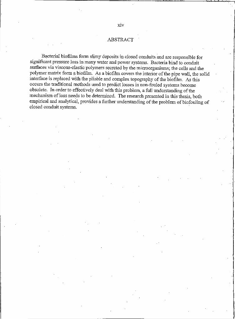
Abstract:Bacterial biofilms form slimy deposits in closed conduits and are responsible for significant pressureloss in many water and power systems. Bacteria bind to conduit surfaces via viscous-elastic polymerssecreted by the microorganisms; the cells and the polymer matrix form a biofilm. As a biofilm coversthe interior of the pipe wall, the solid interface is replaced with the pliable and complex topography ofthe biofilm. As this occurs the traditional methods used to predict losses in non-fouled systems becomeobsolete. In order to effectively deal with this problem, a full understanding of the mechanism of lossneeds to be determined. The research presented in this thesis, both empirical and analytical, provides afurther understanding of the problem of biofouling of closed conduit systems.
INCREASE OF FRICTIONAL RESISTANCE IN CLOSED
CONDUIT SYSTEMS FOULED WITH BIOFILMS
by
Mark Douglas Groenenboom
A thesis submitted in partial fulfillment of the requirements for
the degree of
Master of Science in
Mechanical Engineering
MONTANA STATE UNIVERSITY-BOZEMAN Bozeman, Montana
April 2000
/
f i y n
G,n>-4APPROVAL
of a thesis submitted by
Mark Douglas Groenenboom
This thesis has been read by each member of the thesis committee and has been found to be satisfactory regarding content, English usage, format, citations, bibliographic style, and consistency, and is ready for submission to the College of Graduate Studies.
Approved for the Department of Mechanical Engineering
Dr. Doug Cairns __ t(Signature)
Approved for the College of Graduate Studies
Dr. Bruce McLeod(Signature) Date
STATEMENT OF PERMISSION TO USE
In presenting this thesis in partial fulfillment of the requirements for a master’s
degree at Montana State University - Bozeman, I agree that the library shall make it available to borrowers under the rules of the Library.
IfI dictated my intention to copyright this thesis by including a copyright notice
page, copying is allowable only for scholarly purposes, consistent with “fair use “ as
prescribed in the U.S. copyright Law. Request for permission for extended quotation
from or reproduction of this thesis in whole on in parts may be granted only by the
copyright holder. . -
Signature
Date

IV
To my family, friends, and especially to Monica, who has always been there for me.

V
ACKNOWLEDGEMENTS
This project was possible thanks to National Science Foundation.
I would like to thank all the members of my committee and the structure function
group at the Center for Biofilm Engineering. Particularly, Dr. Halulc Beyenal for his
sharing of his wealth of knowledge regarding biofilms. In addition, I would like to thank
John Neuman for his technical assistance. The help was greatly appreciated.
Vl
TABLE OF CONTENTS
LIST OF TABLES............................................................................................................. ix
LIST OF FIGURES............................................................................................................ x
LIST OF VARIABLES....................... xiii
ABSTRACT............... xiv
1. INTRODUCTION........................................... I
Introduction............................................................ IBackground...................................................................................................................2 'Literature Review...........................................................!..............................................8
2. APPROACHES TO REDICTING VELOCITY PROFILES INHETEROGENEOUS BIOFILMS........................................................................... 20
Introduction................................................................................................................. 20Velocity Profile of an Actual Biofilm.............. ,...21Comparison of Flow Velocity within a Biofilm to AtmosphericFlow in a Vegetative Canopy.................................. 23Comparison to Flow within an Artificial Canopy....:................ 28Evaluation of Flow through a Model BiofilmComposed of Cylindrical Elements.................. 33Conclusion.................................................................................................................. 37
3. MATERIALS AND METHODS................................. ...38
Introduction................................................. 38System Layout.......................................................................... 38Growth Medium and Sterilization...... ......................... ....... ,...................................... 41Method of Biofouling....... ............................................................... 42Measurement of Pressure Loss and Calculation of Friction Factors.......... ................43
4. CLOSED CONDUIT SYSTEM HEADLOSS AS AFUNCTION OFBlOFILMSTRUCTURE............................................................... 46
Introduction.........................................................................................................■....... 45Porosity Study............................................................................................................. ,47
a) Porosity Study Materials and Method.............................................................. 47b) Biofilm Imaging and Image Analysis............................................................... 48c) Results of the Porosity Study........................................................................ 48
Experiment to Quantify a Relationship betweenBiofilm Structure and Energy Loss .................................................. 51a) Materials and Methods.......................................................................................51b) Results.................................................................................... 53c) Dimensional Analysis........................................................................................54
Discussion and Conclusion........ .................................................................. ;............57
5. THE PHEOMENON OF INCREASING FRICTION FACTORWITH INCREASING REYNOLDS NUMBERIN BIOFOULED SYSTEMS....................................................................................61
Introduction...................................................................................................;............ 61Experiment Specific Details and Methods......................................................... 64Results........................................................................ 65Experimental Observations..........................................................................................68Discussion....,............................................................... 70Conclusions..................................................................................................................75
6. SIMULATING A FILAMENTOUS BIOFILM SURFACE.... ..................................76
Introduction.,.............................................................................................. 76Materials and Methods.................................................................................................76Results....................................................................................................... 79Discussion................................................................................................................ 80
7. A RELATIONSHIP BETWEEN MEAN FLOW VELOCITY AND FRICTIONFACTORS EXHIBITED BY BIOFOULED SYSTEMS......................................... 82
Introduction..... .................................................................................. 82System Layout and Reactors.......................................................... 82Constrictional Effects...................................................................................................83Results..........................................................................................................................84Discussion............................................................................................................. 86
8. CONCLUSION AND FUTURE WORK................................................ 91
vii
V lll .
REFERENCES CITED.......... :.......................................... ...............................................96
APPENDICES............................................................................................................... 100
APPENDIX A ......................................................................................... • ........... io iSpreadsheet Data / Measurements of Streamer..................................................102Lengths for the Experiment of Chapter 4 ............................................ ........... ...102Sample of Images Taken for the Experiment of Chapter 4 ..'.................. ............103
APPENDIX B ........ ........................ .............:........................................................... 104Spreadsheet Data for Chapter 5 Experiment....................................... ................105
IX
LIST OF TABLES
Table Page
Table 2.1 Attenuation Coefficients for Various Canopies............... .................................26
Table 5.1 Friction Factor Values and Comparison Blasius Solution................................67
Table 7.1 Experimental Parameters for the 12 Experiments............................................83
Table 7.2 Reynolds number, Velocity and MaximumFriction Factor of the 12 Experiments............... .............................................85
LIST OF FIGURES
Figure , Page
Figure I . I Diagram of Forces Acting on a Slug of FluidTraveling through a Pipe........................................ 2
Figure 1.2 The Moody Diagram.................................................. 7
Figure 2.1 Image of 3-Specie Biofilm Showing the Locations atwhich Velocity Profiles Were Measured............................................. 22
Figure 2.2 Plot of Flow Velocity as a Function of Vertical Positionfor the Five Locations Shown in Figure 2.1 ....................,......................... 22
Figure 2.3 Flow Profile Generated by Equation 2.1 with anAttenuation Coefficient of 2 ..................................................................... 24
Figure 2.4 Nondimensional Wind Profiles for Various Canopies...................................25
Figure 2.5 Superimposing of Biofilm Flow Profile on Figure 2.4................. 26
Figure 2.6 Spherical Canopy Illustration........................................................................28
Figure 2.7 Flow Profile Generated using the Canopy Model Composed of Spherical Elements and AssociatedVariables from Stoltzenbach (1989).................................. 30
Figure 2.8 Predicted Flow Profile for Sample Biofilm...................................................32
Figure 2.9 Proposed Cylinder Model......................................................... 33
Figure 2.10 Drag Coefficient as a Function of Reynolds Number for a Cylinder............34
Figure 2.11 Plot of Biofilm Flow Velocity Profile with Plots ofEquation 2.9 for Various Values of B............;..........................................36
Figure 3.1 The General System Layout used for the Experiments ofChapters 4 through 7 ...................................:................. ...........................39
Figure 3.2 Photo of an Actual ClosedConduit Reactor System............................................... '........................... 40
Figure 3.3 An Impeller Pump also used to provide Flow throughthe Recycle Loop and Closed Conduit Reactor........................................ 41
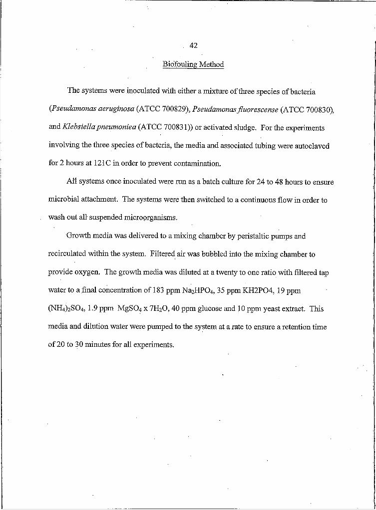
Figure 3.4 Cole Parmer Flowmeter................................................ ............................ ..43
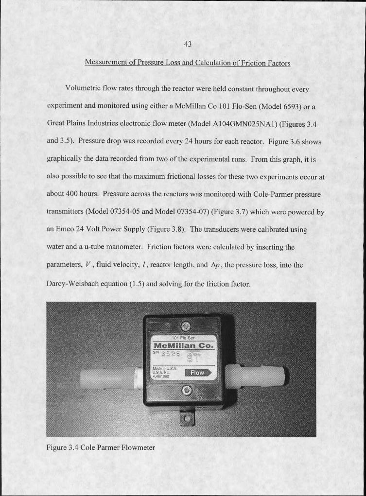
Figure 3.5 GPI Flowmeter.................. ......................... ................ ;.................. ............44
Figure 3.6 Plots of Pressure Loss vs. Time for Two Experiments involving an 8 mm Square Glass Tubeand the Three Species Bacteria................................................................. 44
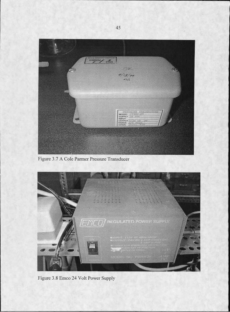
Figure 3.7 A Cole Parmer Pressure Transducer ........... ......................................... .......45
Figure 3.10 The Emco 24 Volt Power Supply used toProvide Voltage to the Pressure Transducers........................................ ...45
Figure 4.1 Porosity Profile Graph Showing Low Porosity at the Biofilm Base........... 49
Figure 4.2 Close-Up Image of Substratum and Biofilmwith Filaments Protruding Toward the Bulk............................................ 50
Figure 4.3 Typical Sample of %” I.D. Vinyl Tubingfrom Second Experiment.................... 52
Figure 4.4 Image of Sample Showing the Traces used toMeasure the Filament Lengths and Base Thickness................................. 52
Figure 4.5 Non-Submerged Sample with Filaments Adhered to the Base Film........... 53
Figure 4.6 Plot of Friction Factor vs. Dimensionless Factor ofStreamer Length / Conduit Length........................................................... 53
Figure 4.7 Plot of Biofilm Thickness vs. Friction Factor.............................................. 53
Figure 4.8 Plot of Friction Factor vs. Dimensionless Factor of StreamerLength / Conduit Length........................................................................... 57
Figure 5.1 Graph Comparing the Friction Factor Generated by theNon-Fouled Vinyl Reactor to the Friction Factor PredictedUsing Tradition Methods for a Hydraulically Smooth Pipe..................... 66
xi
X ll
Figure 5.2 Plot of Friction Factor vs. Reynolds Number forVarious Days of Growth Riofilm..................................... .........................68
Figure 5.3 Images of the Cross-Sections Removed from Experiment..........................69
Figure 5.4 Side Views of Cross-Sections Taken from the Experimenton day 7 and 32..................................... ................. ..................................70
Figure 5.5 Illustration of Flow Profile without the Presence ofFilamentous Biofilm and Proposed Velocity Profile forConduit Fouled with Filamentous Riofilm..................... ..........................72
Figure 5.6 Graph Showing the Dramatic Difference in the Friction Factors for the Clean Reactor and the Reactor fouled with 22 days of Biofilm Growth...............................................................73
Figure 6.1 Images of Simulated and Naturally Biofouled conduit................................ 77
Figure 6.2 Image of a Cross Section of the Tube Lined with the AcrylicFur with Measurement Showing the Hydraulic Diameter............. ...........78
Figure 6.3 Plot of Friction Factor vs. Reynolds Number for the ConduitLined with the Artificial with the Acrylic Fur ...........................................79
Figure 6.4 Plot of the Friction Factor vs. Reynolds Number forBiofouled and Non Fouled Conduit................................................... 80
Figure 7.1 Graph Illustrating the Relationship between ReynoldsNumber and Maximum Friction Factors Exhibited by the Fouled Closed Conduit Reactors......................................................... 85
Figure 7.2. Plot Comparing Mean Flow Velocities toMaximum Friction Factors....................................................................... 86
Figure 7.3 Biofilm Structure for Bulk Fluid Velocity of 1.33 m/s................................ 89
Figure 7.4 Biofilm Structure for Bulk Fluid velocity of 2.85....................................... 89
xiii
LIST OF VARIABLES
j[ = Cross Section Area of Cylinder a = Attenuation Coefficient aK = Kouwen Equation Coefficient d = Maximum Sphere Radius a = Minimum Sphere Radius A = Kouwen equation coefficient Cd = Coefficient of Drag C = Skin Friction CoefficientD = Hydraulic Diameter n = Effective Diameterl j Off
EI = Bending Stiffness f = Friction Factor g = Gravitational Acceleration h = Roughness Heights k = Kouwen Roughness Height
= Canopy Height = Head Loss
I = Conduit Length L = Length M =MassH = Number of Cylinders Per Area
= Exit Pressure
t = Timeu = Fluid Velocity within Canopyu = Wall Friction Velocityjj, = Open Channel flow VelocityUh = Velocity within CanopyUh =V elocity at Canopy Top y = Mean Conduit Fluid Velocity Volejf = Effective Volume z — Height within Canopyr = Conduit Wall Shear Stressa = Sphere Volume Fraction# = Ratio of Average Sphere Radius to
. Canopy Height§ = Absolute Boundary Layer Thickness§* = Displacement Layer ThicknessEpl = Pressure Loss per Conduit Length£ = Average Roughness Heightjl = Kinematic Viscosityp = Fluid DensityQ = Momentum Layer ThiclcnessH = Dimensionless Pi Group
p. = Inlet PressureRe = Reynolds NumberSlam = Average Streamer LengthSI = Streamer Length Per Conduit Length
XlV
ABSTRACT
Bacterial biofilms form slimy deposits in closed conduits and are responsible for significant pressure loss in many water and power systems. Bacteria bind to conduit surfaces via viscous-elastic polymers secreted by the microorganisms; the cells and the polymer matrix form a biofilm. As a biofilm covers the interior of the pipe wall, the solid interface is replaced with the pliable and complex topography of the biofilm. As this occurs the traditional methods used to predict losses in non-fouled systems become obsolete. In order to effectively deal with this problem, a full understanding of the mechanism of loss needs to be determined. The research presented in this thesis, both empirical and analytical, provides a further understanding of the problem of biofouling of closed conduit systems.
I
INTRODUCTION
Introduction
Bacterial biofilms form slimy deposits in closed conduits and are responsible for
significant pressure loss in water distribution systems and hydraulic lines used in power
generation. Bacteria bind to conduit surfaces via viscous-elastic polymers secreted by the
microorganisms; the cells and the polymer matrix form a biofilm. As a biofilm covers
the interior of the pipe wall, the solid interface is replaced with the pliable biofilm. As
this occurs, the traditional methods used to predict losses in non-fouled systems become
unreliable. In order to effectively deal with this problem, a better understanding of the
. mechanism of energy loss is needed. The research presented in this thesis provides a
better understanding of the problem of biofouling in closed conduit systems.
This chapter explains the traditional approach to the problem of frictional losses in
closed conduit system's. Also presented is a review of the literature relevant to the
specific problem of increased frictional losses related to biofouling. Chapter 2 evaluates
three approaches to modeling flow in highly porous heterogeneous biofilms. Chapter 3
provides the materials and methods used in the laboratory to generate the results given in
Chapters 4 through 7. Chapter 4 quantitatively relates increased frictional losses to
biofilm structure. Chapter 5 investigates an interesting relationship between frictional
2
losses and Reynolds number in systems fouled with biofilm, and Chapter 6 shows the
results of an attempt to artificially simulate the fluid biofilm interface in a closed conduit.
Chapter 7 shows how losses in biofouled systems are better related to fluid velocity than
to Reynolds numbers based on pipe diameters.
Background
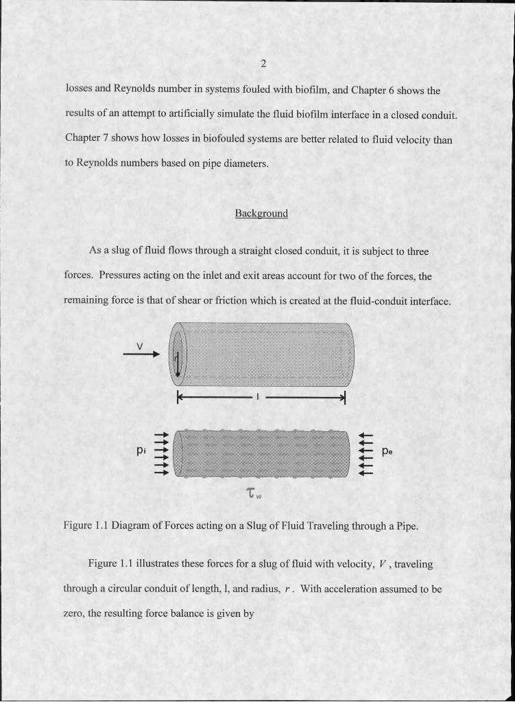
As a slug of fluid flows through a straight closed conduit, it is subject to three
forces. Pressures acting on the inlet and exit areas account for two of the forces, the
remaining force is that of shear or friction which is created at the fluid-conduit interface.
Figure 1.1 Diagram of Forces acting on a Slug of Fluid Traveling through a Pipe.
Figure 1.1 illustrates these forces for a slug of fluid with velocity, V , traveling
through a circular conduit of length, I, and radius, r . With acceleration assumed to be
zero, the resulting force balance is given by
3
p ,nr2 - P eW2 - r w2wl = 0' 1.1
where p; is the inlet pressure, r is the pipe radius, pe is the exit pressure, Tw is the shear
stress caused by the conduit walls, and I is the pipe length. The change or loss in pressure
experienced by the slug of fluid can then be expressed as
1.2r
Equation 1.2 illustrates that the shear force exerted on the fluid by the pipe wall
causes the drop in pressure experienced across the slug of fluid traveling down the pipe.
Equation 1.2 also shows the direct relationship between the length of the pipe and the
pressure loss.
In many engineering applications, it is necessary to predict pressure losses in closed
conduits. Hence, the shear force and resulting pressure loss formed the focus of a
substantial amount of research during the first half of the 20th century. For laminar flow,
predicting losses is relatively simple. By applying the no-slip boundary condition at the
fluid-wall interface, along with the boundary condition of finite velocity at the pipe
center, one can analytically solve for the flow profile [I]. The resulting flow profile for
conduits of circular cross section is parabolic. From this velocity profile, shear is
determined. The results show that for laminar flow, shear stress is linearly related to the
Reynolds number, given by equation 1.3 [2],
Re 1.3
4
where p is the fluid density, V is the fluid velocity, D is the hydraulic diameter, and fi
is the dynamic fluid viscosity. For turbulent flow, no analytical solution is available and
prediction of shear stress and pressure loss is much more complex.
Munson states [2],
“Turbulent flow can be a very complex difficult topic - one that has yet defied a rigorous theoretical treatment. Thus, most turbulent flow analyses are based on experimental data and semi-empirical formulas, even if the flow is fully developed. These results are given in dimensionless form and cover a very wide range of flow parameters, including arbitrary fluids, pipes and flow rates.”
This has indeed been the approach used to predict pressure losses in closed conduit
systems.
In order to form a dimensionless equation applicable to predicting fluid losses in
closed conduits, Darcy and Weissbrook [2] applied the technique of dimensional analysis
to the relevant variables involved with the problem. The relevant variables were
determined to be fluid velocity, V ; fluid viscosity, ju; fluid density, p ; conduit length,
I ; conduit diameter, D, and the roughness of the conduit surface, s . Written
functionally.
A? - F (V ,D ,l,s ,p ,p ) 1.4
The result of the dimensional analysis performed on these variables is the Darcy -
Weisbach equation [2],
D 2 g 1.5
5
where the variables are: H l , the head loss; I ,the pipe length; V ,the average fluid
velocity; g , the gravitation constant, and D is the pipe diameter. The one undefined
variable is f, the friction factor.
For turbulent flow, the friction factor is functionally dependent on a complex
relationship between two other dimensionless quantities, the Reynolds number (equation
1.3) and the relative roughness. Relative roughness is the ratio of the statistically
averaged heights of the roughness elements to the pipe diameter ( s / D ).
A vast amount of empirical and theoretical research was directed toward
quantifying the friction factor during the first half of this century. In 1934, Pigott
compiled the results of over 10,000 experiments from various sources and formed the
Pigott chart [3]; the chart related relative roughness and Reynolds number to the friction
factor. Unfortunately, the data were compiled in such manner that practicing engineers
could not easily extract results. Pigotfs work was followed by Nikuradse who artificially
roughened pipes with sand grains [4]. Because of the substantial difference between
sand-roughened surface and surfaces encountered in practice, Nikuradse’s results varied
substantially from those of Pigott Based on Nikuradse’s results, von Karman and
Prandtl developed theoretical analyses of pipe flow that resulted in numerical constants
for the case of hydraulically smooth surfaces in which the roughness elements are small
compared to the boundary layer thickness [5]. In 1938, Colebrook continued to fit
formulas to the empirical data [5], Unfortunately, Colebrook's equation, like Pigoffs
chart, was cumbersome and difficult for the practicing engineer to use. Also in 1938,
6
Blasius [2] offered a solution that was much more tractable but only applicable to
hydraulically smooth surfaces.
In 1944, Lewis F. Moody [5] compiled the results of previous researchers in order
to “furnish the engineer with a simple means of estimating the friction factors to be used
in computing the loss of head in clean new pipes”. Moody’s relatively simple technique
of predicting frictional losses has become a standard method used by the practicing
engineer to predict pressure losses in closed conduits.
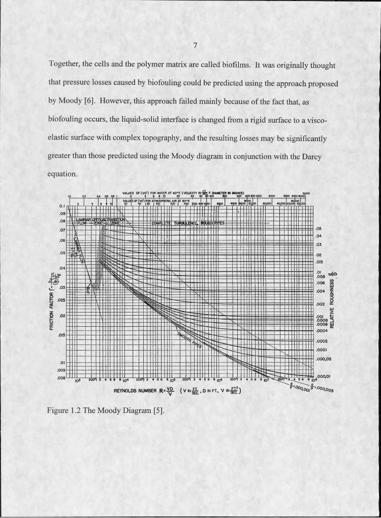
Moody provided a chart similar to Pigotfs that correlates the two dimensionless
quantities of Reynolds number, Re, and relative roughness, s / D , with the friction factor,
f. In addition, Moody provided the engineer with charts for determining the exact value
of relative roughness and Reynolds number for a closed conduit system. Moody’s chart
(Figure 1.2) is then used to correlate these two dimensionless quantities with the friction
factor. The corresponding friction factor is then inserted into the Darcy equation (1.5)
together with the fluid velocity, hydraulic diameter and length. With these parameters,
the Darcy equation can predict losses in clean, new systems to within 5%.
However, Moody's diagram is applicable only to “clean new pipes” [5], Many old
piping systems (and those prone to microbial fouling) exhibit substantial losses that
cannot be predicted using this traditional diagram.
Microbial fouling (biofouling) is a technical term referring to the adverse effects
caused by the attachment of microorganisms to liquid-solid interfaces. These
microorganisms, i.e. bacteria, bind to a surface and each other via viscous-elastic
extracellular polymers made mainly of polysaccharides produced by the bacterial cells.
7
Together, the cells and the polymer matrix are called biofilms. It was originally thought
that pressure losses caused by biofouling could be predicted using the approach proposed
by Moody [6], However, this approach failed mainly because of the fact that, as
biofouling occurs, the liquid-solid interface is changed from a rigid surface to a visco
elastic surface with complex topography, and the resulting losses may be significantly
greater than those predicted using the Moody diagram in conjunction with the Darcy
equation.
(VO*) FOR WATER AT 60*F (VELOCITY IN-Sfc 4 6 e Ip ep 40 eo ap
X OlAMETOt M HOMES)VALUES OF
T O iB IL E
.004
.0008 5
.0006 W
.0004
0 0 0 2
.0001
.000,05
2(10* 3 4 5 6 8 |q 72(10*) 3 4 5
REYNOLDS NUMBER R = X L ( v IN^L , D IN FT, V INggg)
Figure 1.2 The Moody Diagram [5],
8
Literature Review
McEntee did some of the earliest study into the energy losses caused by biofouling'
in 1915 [7], McEntee submerged a series of steel plates in water, allowed a biofilm to '
form on the plates, and then tested them for frictional resistance to fluid flow. He
concluded that the biofouling resulted in a 2% increase in frictional resistance each day
the biofilms were allowed to grow. In a discussion of McEntee’s.paper, Sir Archibald
Denny, a member of the Society of Naval Architects and Marine Engineers,
acknowledged a similar increase in frictional resistance. He stated, “for each day a vessel
lies in our dock the skin friction resistance increases at a rate of 1A0Zo per day and this we
have found to be true for periods as long as three months.” [7],
Other areas where the increase of frictional resistance is troublesome is in the ■
water-supply and power industries. Such systems are particularly prone to biofouling,
due to an abundance of bacteria. Observations of researchers investigating biofouled
industrial systems have been qualitative with regards to biofilm structure, and
quantitative with regard to energy losses caused by the biofilms.
In a case in 1959, biofouling affected a power conduit located in North Carolina [8].
The pipeline, put into operation in 1928, was approximately 4.75 miles long, and was
composed of both steel and concrete sections. In 1928, the conduit friction head losses
were determined to be 40.6 feet at 900 cfs. In 1945, the conduit friction head losses had
increased to 55 feet, i.e. 35% greater than the original value. In 1945, inspection of the
11-ft diameter pipeline found the steel pipe portion of the line, which was painted with
bituminous paint in 1939, to be in excellent condition. The inspection also showed no
9
structural damage to the concrete lining, however, the concrete portions were found to be
covered with “something like a dense layer of soot” [8], These rough black fouling
deposits were up to 5Zg inch thick and had an average depth of 1A inch overall. Chemical
analysis showed that these deposits were composed of 87% water and organic matter,
2.5% organic matrix and 10.5% mineral matter. It was also observed that the deposits
consisted of layers that “undoubtedly represent equilibrium conditions and are obviously
laid down at yearly intervals” [8]. The researchers assumed microorganisms (i.e.
biofilm) formed the deposits, and the goal of the research was to determine the best
method of treatment. The authors concluded that mechanical cleaning at certain intervals
was the most cost-effective solution. Although knowledge of the composition of these
deposits may be helpful in determining effective temporary solutions to the biofouling
problem in closed conduits, this knowledge does nothing to associate biofilm structure to
the resulting effect on fluid dynamics and the resulting losses.
Another notable case of this type of fouling occurred in Germany in 1950. In this
instance, a 60-cm diameter, 93-kilometer long water supply line was reduced to 55% of
its original flow capacity over three years. The loss was due to a “thin, slimy layer” [9].
The layer was characterized by a “ripple-like” surface having an average thickness of .
0.25-in. The resulting energy losses could not be explained in terms of constriction or
equivalent sand roughness common to friction factor relationships.
Regarding this particular case, Characklis pointed to the rippled surface as the cause
of the unusually high losses experienced by pipelines,, using an example of a solid surface
of similar pattern that showed high frictional resistance [10]. Brauer performed
10
experiments on form stability of asphalt-lined pipes as a function of temperature of the
flowing water [11]. Brauer observed that, at higher temperatures, the asphalt mating also
assumed a rippled surface structure, which was accompanied by an unusual increase in
frictional resistance. Brauer proposed that there is a “two phase” flow, in which shear
stress (caused by the bulk fluid flow acting on the asphalt) forced the asphalt to be
dragged along the pipe wall [11]. Although this theory would explain an increase in loss,
Characklis acknowledges that the losses are not nearly as high as the losses occurring in
some biofouled systems.
Characklis continues with a general explanation of energy loss in turbulent flows
past rigid surfaces.
“The complicated nature of turbulent motion can be visualized by assuming that fluid particles moving near the wall coalesce into lumps and travel bodily together for a certain distance. If such a lump of fluid collides with the leading part of a roughness element, the fluid changes its direction and a momentum exchange takes place. Any forced motion of the fluid particles in a direction transverse to the flow corresponds to an increase in general turbulence. This phenomena causes energy loss in flow past rigid rough surfaces” [12].
Characklis then explains a possible mechanism for increased losses in biofouled
systems when the fluid interface is changed from that of a rigid surface to a rippled slime
layer.
“If the material constituting the roughness element has a low modulus of elasticity, the force exerted on the roughness element by the fluid may be sufficient to cause a temporary deformation of the element which would result in an oscillatory motion of the pliable roughness element. A resonance phenomenon could occur from the coordinated motions of the individual roughness elements.”
11
Also in 1973, Kouwen and Unny investigated the effects of surface roughness
flexibility in open channels [13]. They applied dimensional analysis to the situation and
postulated the following relationship (1.6).
U f
N y _i
mEI h d'
^ P u O y
Ik° 1.6
Where U0 is wall friction velocity; U is the free stream velocity; h0 is the roughness height
with an undeflected pliable over-layer; 5 is the height of the absolute boundary layer
(shear layer); h is the measure of the roughness height; EI is a measure of the bending
stiffness'of the pliable elements; and m is a non-dimensional value of the aerial density of
the elements. Kouwen and Unny ultimately proposed the following empirical
correlation, in which aK and bK represent numerical constants.
mEIV
-bs/ 1.7
Minkus reported another case of this phenomenon [14]. This case involved a 42-in.
diameter cast iron pipeline that had been used to transport water 7 miles to a treatment
facility for 22 years. To increase longevity of the line, a 1A-In cement lining was added to
the pipeline wall. Capacity measurements were taken after the lining was applied and
again 2 years later. The results showed a decrease in the pipeline’s capacity from 50
million gallons per day to 44 million gallons per day. Inspection of the pipeline showed
the cement lining to be in excellent condition; “however, a microbiological and chemical
film 1/32 to 1/16 in. thick was found attached to the wall” [14].
12
Minlcus also reports about a 36-in. concrete pipeline that was tested over a 5-year
period. This pipeline showed a reduction in flow of 23%, from 35 millions gallons per
day to 27 million gallons per day [14]. Immediately after emptying the pipeline, a film
was observed, and although it appeared to be smooth, Minkus states that “it could be said
that with a little imagination that there was a rougher feeling to the deposit."
In 1980 Picologlou et al. [6], presented the results of the first formal laboratory
experiments focused on the specific problem of pressure loss in biofouled closed
conduits. Picologlou et al. ran a series of experiments involving three tubular fouling
reactors (TFR) that were fouled with biofilm while pressure loss across the reactors was
monitored. In these experiments, either velocity through the reactor, or pressure loss
across the reactor, was held constant. The experiments in. which velocity was held
constant showed increases in pressure loss, while the experiments with a constant rate of
pressure reduction showed diminished flow capacity. The authors propose and evaluate
six possible mechanisms that could contribute to the increased losses.
I . Biofilm constricting the diameter and reducing flow.
To evaluate the extent and affect of diameter constriction by the biofilm, the authors
measured biofilm thickness during their experiments. Thickness measurements were
determined by dividing the biofilm volume by the surface area covered by the
biofilm. Biofilm volume was determined by removing a sample of biofilm and then
allowing excess fluid to drain from the sample. The authors acknowledge that the
thickness measurements could be as much as 36% larger for drain times of 2.5
minutes than for drain times of 10 minutes. They also found that the constriction of
13
the hydraulic diameter caused by the biofilm would account for only 10% of the total
frictional resistance.
2. Change in fluid viscosity.
The authors found that fluid viscosity never varied by more than 2% from pure
water; therefore, the authors dismissed the effect that fluctuating viscosity had on
pressure loss as negligible.
3. Viscous dissipation within the biofilm due to its creeping flow in the down stream
direction.
The authors refer to the work done by Bauer [11] regarding the asphalt-lined
conduits, but dismiss this creeping phenomenon as a possible mechanism for the
increase loss based on two reasons. First, the biofilm coverage always appeared
uniform, and second, there was no evidence of an accumulation of biofilm in areas
where creeping biofilm would collect.
4. Viscous dissipation within the biofilm due to its oscillatory response to turbulent
flow excitation.
Previous research by the authors determined the viscoelastic nature of the biofilm.
Using a Weissenberg Rheogoniometer, the biofilm was determined to have a
relatively large viscous modulus, i.e., the viscous modulus was much larger than the
elastic modulus. Picologlou et al. state that, “the possibility exists that the biofilm
draws energy from the flow, such energy being eventually dissipated through viscous
action. This situation is quite complex and defies analysis, particularly since there is
a nonlinear coupling between the structure of the turbulent flow and the biofilm
14
response.” The authors also believe that this loss mechanism is of secondary
importance because the losses they observed could quite satisfactorily be attributed to
increased film surface roughness.
5. Increased dissipation in fluid due to increased surface roughness as a result of
biofilm accumulation.
Although the frictional resistance observed could usually be adequately explained
using methods for rigid rough surfaces, the authors do not conclude that the biofilm
presents a rigid rough surface to the flow. This would be an oversimplification and
would not account for all their experimental observations. Specifically, in one
experiment the pronounced frictional resistance could not be adequately explained as
a rigid surface element.
6. Increased dissipation in fluid due to the presence of biofilm filaments.
Filaments of the biofilm were observed to flutter with a frequency related to the
bulk fluid velocity. The authors also qualitatively observed that the frictional
resistance increased with increasing filament length, although they do not define what
is meant by “streamer length”. They suggest that this loss mechanism is analogous to
increased drag in streams due to bottom vegetation, and similar phenomena occurring
in atmospheric boundary layers in the presence of natural vegetation.
The authors concluded that both frictional resistance and equivalent sand roughness
values correspond to an increase in biofilm thickness. They characterized the frictional
losses as having a lag period associated with small biofilm thickness, followed by a rapid
increase when the biofilm thickness reached a critical thickness. The authors
15
hypothesized that this may be because the biofilm thickness reaches a critical value in
relation to the viscous sublayer thickness. The response of the friction factor for a tube
with attached biofilm is similar to that of a rigid rough surface for Reynolds numbers
ranging from 5,000-48,000. They also observed a filamentous morphology of the biofilm
surface and stated that these filaments contribute to the increase in frictional resistance.
Many researchers have suggested that biofilms have an effect similar to that of a
compliant surface [6], [10], [15], [16], [17-21], Most research done in this area suggests
compliant surfaces reduce skin friction, in some cases, significantly. These findings tend
to contradict applying such a concept to biofilms. Initial research in this area was done
by Kramer, who covered underwater projectiles with rubber diaphragm [19]. He found
drag could be reduced up to 40% from that of an equivalent rigid-surface projectile at
Reynolds numbers of 15x106. Looney and Blick achieved reductions in skin friction up
to 50% using a compliant plane [20]. Pelt found reductions of 35% in friction losses for
flexible tubes lined with a variety of viscous fluids [21]. The findings of all of this
research suggest that to maximize reduction in drag, a highly viscous fluid enclosed by
the thinnest membrane should be used.
Research by Klinzing et al. [22] on frictional losses in foam-damped flexible tubes
yielded interesting but inconclusive results. They tested flow through a 15/16-in inner
diameter, 1/16-in wall silastic tube. This tube was encased by polyurethane foam, and
was hydraulically smooth. Although no pronounced decrease in frictional resistance was
found, the authors do show a definite decrease in the friction factor for the foam-damped
tube between Reynolds numbers of 10,000 and 20,000. They interpret this result as a
16
possible delay in the onset of full turbulence from the normal transition range of
Reynolds numbers between 2100 - 7000 to the 10,000 - 20,000 range.
Loeb et al. [17] studied the effects of microbial fouling films on the hydrodynamic
drag of rotating disks. This experimental study was undertaken to “evaluate the effects of
■ microbial slime under hydrodynamic conditions that reflect realistic ranges of vessel
operation”. Their work indicated that even under relatively high Reynolds numbers,
representing vessel speeds of 20 to 60 knots, the biofilms increased drag by up to 10%. It
should be noted that they tested surfaces that were either initially hydraulically smooth or
rough. Unlike Picologlou et al. [6], Loeb et al. [17] did not find an initial reduction in
drag on the hydraulically rough discs in the early stages of fouling. •
Lewkowicz and Das [23] investigated turbulent boundary layers on rough surfaces
with and without a pliable over-layer that simulated marine biofouling. They covered
two flat plates (30 cm by 92 cm) with abrasive paper and mounted tufts of fine nylon
fibers to one a plate to form a “combined roughness.” Each tuft contained approximately
300 fibers that were 2 cm long and 15 microns in diameter (the modulus of elasticity for
the nylon is approximately 2 x IO9 N/m2). The tufts were laid out on the plate at a rate of
3100 per square meter. The plate was then placed in a wind tunnel and exposed to a free
stream of air at 26 m/s. By utilizing a flexible top wall in the working section of the
tunnel, the investigators were able to keep the static pressure distribution along the plate
constant to within 2% of the inlet dynamic pressure. “Not surprisingly, the combined
roughness had a thickening effect on the boundary layer (by some 25-30%). Notably, it
affected, in that sense, the displacement thickness more than the momentum thickness as
17
the shape factor, 5* /6 ,fox the combined roughness increased on average by 30%.”
Here <5* is the displacement thickness, and O is the momentum thickness. They also
found the skin friction coefficient, Cf, was 18% higher on the plate with the combined
roughness.
Lewandowski and Stoodley [15] also observed an increase in pressure loss in
conduits fouled with biofilm. They postulated that “structural development of the biofilm
suggests that individual microcolonies behave like blunt bodies shedding vortices. The
microcolonies assume elongated forms, termed “streamers”, possibly because of an
external pressure drag force.” The vortex sheet formed around the blunt colonies
activated the streamers into motion. Energy then dissipated through the flow-induced
movements of the streamer and microcolonies. This would, in part, explain the increase
in pressure loss.
In addition, Lewandowski and Stoodley also suggest that the biofilm influences
pressure loss only above a certain critical flow velocity [15]. This pressure loss,
attributed to the biofilm, reaches a steady (or pseudo-steady) state in the reactor. The
authors conclude that the “interpretation of classical hydrodynamic parameters such as
Reynolds number, friction factor, and surface roughness as related to biofilms should be
reexamined in context to biofilm viscoelasticity and heterogeneity.” The authors also
suggest that, although the Reynolds number calculated using the reactor geometry may be
useful for predicting the overall flow stability, it should be re-evaluated to asses local
flow conditions near a biofihn.
18
To verify their hypothesis concerning the vorticies, the. investigators attempted to
relate the frequencies of streamer motion to the Strouhal number [16]. Using confocal
scanning laser microscopy, they were able to plot the position of a location on a streamer
filament as a function of time. Unfortunately, no characteristic frequencies were found,
suggesting that the streamers’ motion is more likely a response to turbulent flow rather
than to vortices formed around the blunt colonies.' . -
Recently, in 1999, Schultz and Swain investigated the effect of biofilms on
turbulent boundary layers [24]. Their experiments were conducted in a water tunnel
utilizing actual biofilms. Biofilms were grown on steel plates, 2.06-m by 0.58-m (54 mm
thick), in filtered lagoon water. The control plates were non-fouled. The biofilms were
allowed to grow for 2 to 3 weeks, and thickness measurements (performed using a wet-
film paint thickness gauge) ranged from 25 microns to 2032 microns. A fiber-optic laser
Doppler velocimeter (LDV) was used to acquire velocity measurements.
Results of the investigation showed that there was no statistically significant
difference in the turbulent boundary layer (absolute) thickness between the control and
the fouled specimens. However, statistically significant increases in the displacement
thickness and the shape factor were found for the biofouled plates. The authors also
found that the skin friction was dependent on biofilm thickness, composition, and
morphology. For example, a biofilm thickness of 160 microns increased frictional
resistance by 33%, while a thickness of 350 microns increased the resistance by 68%. In
addition, the authors state that biofilms containing a higher proportion of algae seem to
19
“draw a greater amount of momentum from the mean flow” because of “waving algae
filaments”.
The authors conclude that there is not a sufficient characteristic length scale.
associated with the complex biofilm structure to relate it to traditional methods, such as a
standard Nikuradse sand roughness.
Clearly, the problem of increased frictional resistance caused by biofilm has been
the center of a considerable amount of research. Although documentation of the problem
is extensive, there does not currently exist an accepted mechanism relating the biofouling
to the increased losses. The following research was done to provide a clearer
understanding of the relationship between this type of biofouling and increases in
frictional resistance.
APPROACHES TO PREDICTING VELOCITY PROFILES IN HETEROGENEOUS BIOFILMS.
Introduction
To model flow velocities within a biofilm, one must obtain some knowledge of
biofilm structure. There are currently three models of biofilm structure explained in
literature on biofilms grown under low flow velocities.
1. Dense, or slab, biofilm structure, in which there are no pores or voids [25].
2. Heterogeneous biofilm structure, in which microcolonies form mushroom like
structures [26] [27] [28] [29].
3. Heterogeneous mosaic biofilm structure, in which individual microcolonies
form stacks which are separated from other colonies [30].
In the dense or non-porous films, there is no convective flow to model. However,
in the heterogeneous and heterogeneous mosaic structure models, convective transport is
important. Evaluations of three possible approaches to modeling flow within these types
of films are offered in this chapter.
The first evaluation compares the biofilm’s velocity profile to actual profiles
obtained for various vegetative canopies [31]. The second comparison is based on
modeling the film structure as a highly idealized canopy composed of spherical elements
21
[32]. A third possibility of a canopy composed of idealized cylinders is then offered and
evaluated.
Velocity Profile of an Actual Biofilm
In order to evaluate the effectiveness of these approaches, an actual velocity profile
is needed for comparison. The profile that will be used for this purpose was generated at
Montana State University’s Center for Biofilm Engineering using an electrochemical
technique [33]. This technique utilizes the measuring of the limiting current of a
microelectrode. The limiting current is a function of the mass transfer boundary layer,
which is in turn a function of the local flow velocity. The micro-electrode was calibrated
using a particle tracking technique in conjunction with confocal scanning laser
microscopy. The microelectrode was then positioned in and near a heterogenous biofilm.
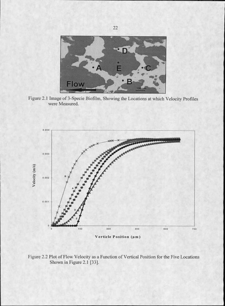
Xia et al. [33] determined velocity profiles at five points (see Figure 2.1) in a three
species biofilm (Psuedamonas aeruginosa. Pseudomonas flour escens and Klebsiella
pneumoniae), which was, on average, 160 pm thick. Four of the five profiles were taken
at voids in the biofilm structure, while the fifth (point E) was taken within and above a
cell cluster. In Figure 2.1, lighter areas denote voids and darker areas represent biofilm
clusters. The velocity profile at point A was selected as the profile to be used for
comparison because of its location in a void and the corresponding flow profile, shown in
Figure 2.2.
Vel
ocit
y (m
/s)
2 2
Figure 2.1 Image of 3-Specie Biofilm, Showing the Locations at which Velocity Profiles were Measured.
V e r t i c l e P o s i t i o n ( g m )
Figure 2.2 Plot of Flow Velocity as a Function of Vertical Position for the Five Locations Shown in Figure 2.1 [33].
23
Comparison of flow velocity within a biofilm to atmospheric flow in a vegetative canopy
Research and studies into flow profiles in natural canopies is abundant. Empirical
data is available for flow profiles from plant types ranging from immature com to large
trees [31]. Such data has been incorporated into the modeling of shear stresses on
vegetation caused by wind gusts, and into complicated models used to predict the
behavior of wildfires. The intent here is to evaluate whether such canopy profiles could
be used to model flow within a porous biofilm.
Arguments can be made both for and against modeling flow within biofilms as flow
within natural canopies. An argument for such a model is that certain components of the
systems are somewhat analogous: flow in both systems can be considered
incompressible, and both canopies are composed of flexible elements. Arguments can
also be made that both vegetation and bibfilms develop structures that optimize nutrient
uptake. For a vegetative system this includes such parameters as sunlight uptake by leaf
area (photosynthesis) and transport of water from the soil throughout the plant. For a
biofilm these processes include breaking down substrates through diffusion and cell
respiration.
At the same time obvious differences exist between the two systems. For instance,
the volume ratios of the two systems vary significantly. For vegetation the ratio of
vegetative volume to total volume is of the order IO'3, while volume ratios of biofilms
with their extra-cellular matrix tend to be of the order IO"1. It follows from this
volumetric relationship that the two systems will also have dramatically different surface
24
area ratios. Differences in these ratios will result in different shear and pressure drag
forces exerted on the fluid in each system.
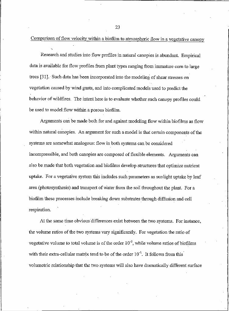
For vegetative canopies, Cionco [31] proposed the following equation for flow
profiles within vegetative canopies,
~~—11u = Ufl * e 2.1
where u is the velocity of the fluid at a given height (z) within the total canopy height
(H). Uh is the fluid velocity at the canopy top, and “a” is an attenuation coefficient that
varies based on the type of vegetation. In order to illustrate the resulting velocity profile.
Figure 2.3 is provided for a canopy with an attenuation coefficient value, a, of two.
10.8
x 0.60.4 0.2
00 0.2 0.4 0.6 0.8 1
u/Uh
Figure 2.3 Flow Profile Generated by Equation 2.1 with an Attenuation Coefficient of 2.
Equation 2.1 is empirically based, and it was developed by fitting curves to data
such as that offered in Figure 2.4. Figure 2.4 shows velocity as a function of vertical
position inside a canopy for several types of vegetation [31]. From this graph one can
observe the similar shape of the flow profiles typical in all vegetation. Also, one should
note that this graph shows the resolution of the flow profiles into the bulk fluid flow up to
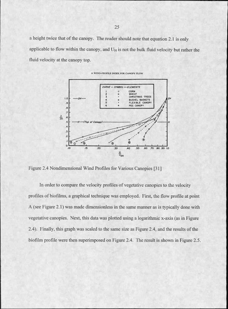
25
a height twice that of the canopy. The reader should note that equation 2.1 is only
applicable to flow within the canopy, and Uh is not the bulk fluid velocity but rather the
fluid velocity at the canopy top.
A WIND-PROFILE INDEX FOR CANOPY FLOW
CURVE — SYMBOL— ELEMENTS
1 o CORN2 » WHEAT3 + CHRISTM AS TREES4 * BUSHEL BASKETS5 * FL E X IB L E CANOPY6 * PEG CANOPY
--- 2H---
-H------- (Top o f Canopy)-
.6 0 .7 0 .8 0 .9 0 IjO
Figure 2.4 Nondimensional Wind Profiles for Various Canopies [31]
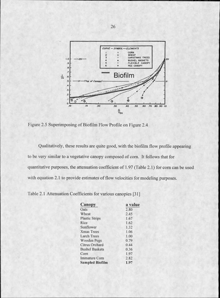
In order to compare the velocity profiles of vegetative canopies to the velocity
profiles of biofilms, a graphical technique was employed. First, the flow profile at point
A (see Figure 2.1) was made dimensionless in the same manner as is typically done with
vegetative canopies. Next, this data was plotted using a logarithmic x-axis (as in Figure
2.4). Finally, this graph was scaled to the same size as Figure 2.4, and the results of the
biofilm profile were then superimposed on Figure 2.4. The result is shown in Figure 2.5.
2 6
CURVE — SYMBOL— ELEMENTS
CORNWHEATCHRISTMAS TR EES BUSHEL BASKETS FLEX IB LE CANOPY PEG CANOPY
— — 2H --------
Biofilm- ----------H ------- (Top o f Canopy)-
.6 0 .7 0 .8 0 .9 0 1.0
U2H
Figure 2.5 Superimposing of Biofilm Flow Profile on Figure 2.4
Qualitatively, these results are quite good, with the biofilm flow profile appearing
to be very similar to a vegetative canopy composed of corn. It follows that for
quantitative purposes, the attenuation coefficient of 1.97 (Table 2.1) for corn can be used
with equation 2.1 to provide estimates of flow velocities for modeling purposes.
Table 2.1 Attenuation Coefficients for various canopies [31]
Canopy a valueOats 2.80Wheat 2.45Plastic Strips 1.67Rice 1.62Sunflower 1.32Xmas Trees 1.06Larch Trees 1.00Wooden Pegs 0.79Citrus Orchard 0.44Bushel Baskets 0.36Com 1.97Immature Com 2.82Sam pled Biofilm 1.97
27
It should be noted that although the fit for the biofilm profile is satisfying visually,
attempts to numerically fit data to equation 2.1 result in a poor correlation. This results
from the difference in the basic shape of the two curves, i.e. the velocity within the
vegetative canopies are concave up while the biofilm’s velocity profile is concave down
(see Figure 2.5).
After these considerations, three conclusions are made for comparing flow within a
biofilm to flow within a vegetative canopy:
1. This approach can be used satisfactorily to estimate the flow velocity within
and above a porous biofilm.
2. Although qualitative comparison is satisfactory, there exists a difference in
the shape of the two profiles, which makes quantitative comparison difficult.
3. Use of equation 2.1, with an attenuation coefficient of 1.97, can provide
approximate flow velocities within, biofilms modeled as heterogeneous and
heterogeneous mosaic films.
2 8
Comparison to Flow within an Artificial Canopy
The previous study compared flow within biofilm systems to flow within a
vegetative canopy. This is primarily an empirical approach to simplify the quantifying of
complicated systems; nevertheless, it does provide researchers with a simple approach for
estimating shear within biofilms.
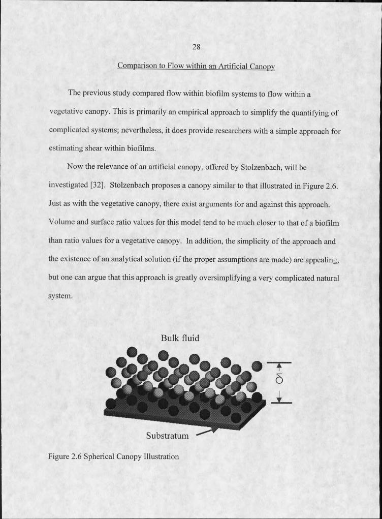
Now the relevance of an artificial canopy, offered by Stolzenbach, will be
investigated [32]. Stolzenbach proposes a canopy similar to that illustrated in Figure 2.6.
Just as with the vegetative canopy, there exist arguments for and against this approach.
Volume and surface ratio values for this model tend to be much closer to that of a biofilm
than ratio values for a vegetative canopy. In addition, the simplicity of the approach and
the existence of an analytical solution (if the proper assumptions are made) are appealing,
but one can argue that this approach is greatly oversimplifying a very complicated natural
system.
Bulk fluid
Figure 2.6 Spherical Canopy Illustration
29
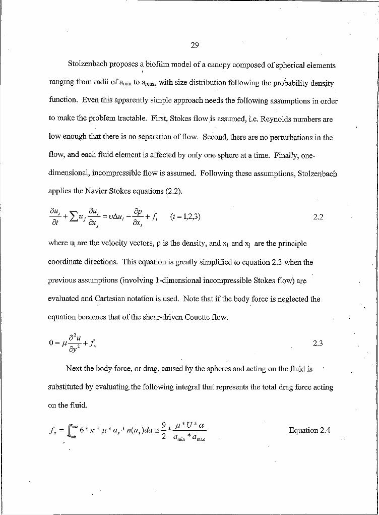
Stolzenbach proposes a biofilm model of a canopy composed of spherical elements
ranging from radii of amj„ to amax, with size distribution following the probability density
function. Even this apparently simple approach needs the following assumptions in order
to make the problem tractable. First, Stokes flow is assumed, i.e. Reynolds numbers are
low enough that there is no separation of flow. Second, there are no perturbations in the
flow, and each fluid element is affected by only one sphere at a time. Finally, one
dimensional, incompressible flow is assumed. Following these assumptions, Stolzenbach
applies the Navier Stokes equations (2.2).
where u; are the velocity vectors, p is the density, and xj and Xj are the principle
coordinate directions. This equation is greatly simplified to equation 2.3 when the
previous assumptions (involving I-dimensional incompressible Stokes flow) are
evaluated and Cartesian notation is used. Note that if the body force is neglected the
equation becomes that of the shear-driven Couette flow.
Next the body force, or drag, caused by the spheres and acting on the fluid is
substituted by evaluating the following integral that represents the total drag force acting
on the fluid.
2.2
2.3
f x = 6* ft* pi* as * n(as )da = - Equation 2.4
30
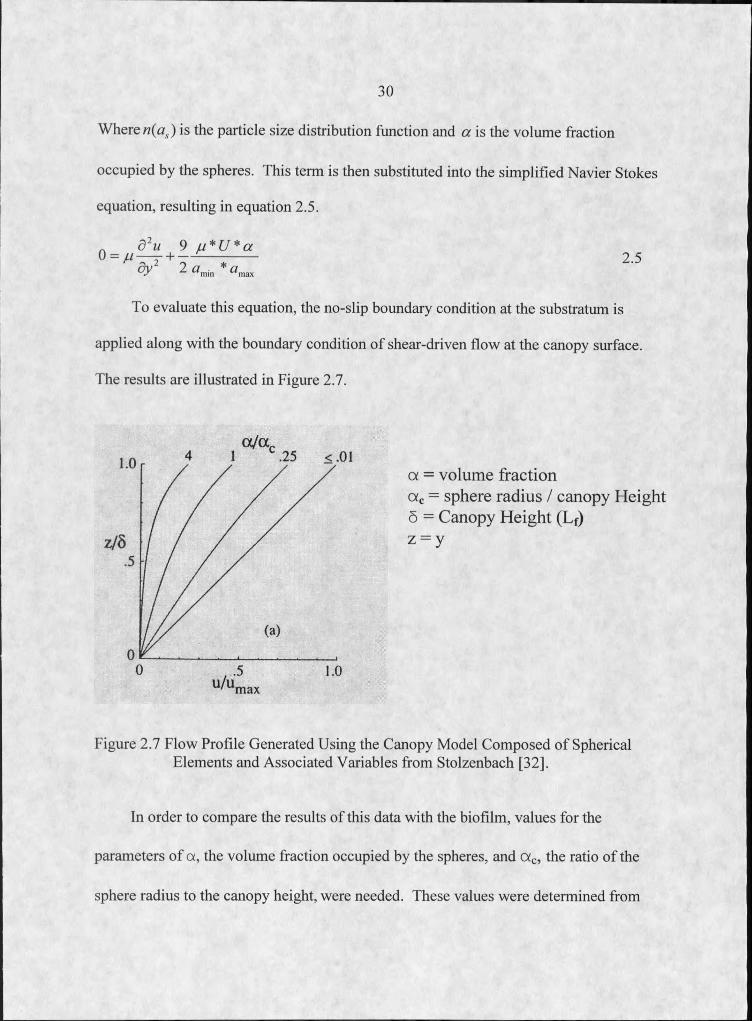
WherertO1) is the particle size distribution function and a is the volume fraction
occupied by the spheres. This term is then substituted into the simplified Navier Stokes
equation, resulting in equation 2.5.
A S2W 9 ju*U *a0 = + ------ 2.5
To evaluate this equation, the no-slip boundary condition at the substratum is
applied along with the boundary condition of shear-driven flow at the canopy surface.
The results are illustrated in Figure 2.7.
m a x
a = volume fraction a c = sphere radius / canopy Height 5 = Canopy Height (Lf) z = y
Figure 2.7 Flow Profile Generated Using the Canopy Model Composed of Spherical Elements and Associated Variables from Stolzenbach [32].
In order to compare the results of this data with the biofilm, values for the
parameters of a, the volume fraction occupied by the spheres, and a c, the ratio of the
sphere radius to the canopy height, were needed. These values were determined from
31
measurements taken from Figyre 2.1. The value for the sphere radius (200 microns) was
taken across the colony where point E is located in Figure 2.1. The thickness of the film
5, was reported to be 160 microns [33]. The value for a, the volume fraction of the film
was estimated to be 0.375. This number was determined by averaging the volume
fraction at the substratum with the volume fraction at the biofilm surface. At the
substratum the volume ratio was estimated to be 0.75. This value is based on the ratio of
the area shown in Figure 2.1 that is covered with biofilm compared to the total area. At
the biofilm surface, the porosity is zero. The average of these, 0.375, was used for the
calculation of the volume fraction, a. To estimate oic (the ratio of the sphere radius
squared to the biofilm thickness squared) the values for the radius of the colony and
biofilm thickness were used. Using these values, a/ac is 0.24, and the estimated profile
shape for this value can be approximated as 0.25. The corresponding curve can be
viewed in Figure 2.7.
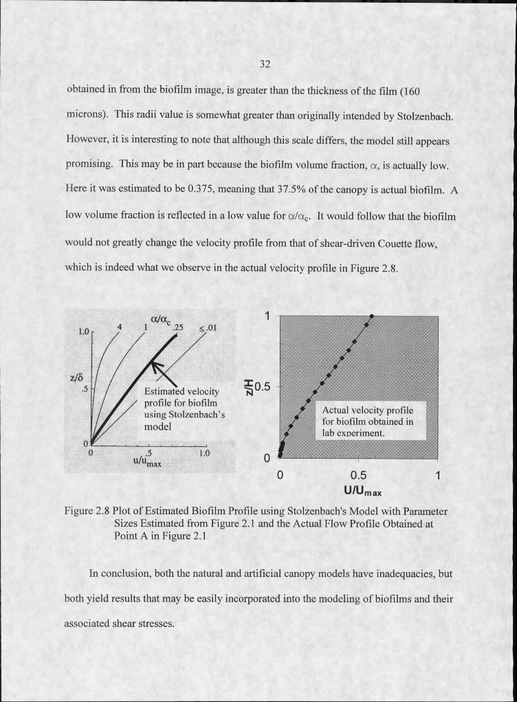
Stolzenbach1 s model compares favorably to the shape of the actual flow profile
generated from the sample data taken from the three species biofilm, and this comparison
can be seen in the 2 graphs in Figure 2.8. Here the data for the actual biofilm was
normalized in the same fashion as Stolzenbach1 s predicted profiles displayed in Figure
2.7. It also interesting to note that flow within the biofilm at point A (Figure 2.1) does
not seem to be greatly affected by the presence of the film.
When the values, which were estimated from the biofilm image, are used to
determine a /ac, the results of this evaluation are favorable. But it needs to be
acknowledged that the estimated value of 200 microns for the value of the sphere radii.
32
obtained in from the biofilm image, is greater than the thickness of the film (160
microns). This radii value is somewhat greater than originally intended by Stolzenbach.
However, it is interesting to note that although this scale differs, the model still appears
promising. This may be in part because the biofilm volume fraction, a, is actually low.
Here it was estimated to be 0.375, meaning that 37.5% of the canopy is actual biofilm. A
low volume fraction is reflected in a low value for a/ac. It would follow that the biofilm
would not greatly change the velocity profile from that of shear-driven Couette flow,
which is indeed what we observe in the actual velocity profile in Figure 2.8.
Estimated velocity profile for biofilm using Stolzenbaclfs model
max
Figure 2.8 Plot of Estimated Biofilm Profile using Stolzenbach's Model with Parameter Sizes Estimated from Figure 2.1 and the Actual Flow Profile Obtained at Point A in Figure 2.1
In conclusion, both the natural and artificial canopy models have inadequacies, but
both yield results that may be easily incorporated into the modeling of biofilms and their
associated shear stresses.

33
Based on the promising results obtained for this model and acknowledging its
insufficiencies, a more appropriate model consisting of cylinders rather than spheres is
offered and evaluated.
Evaluation of Flow Through a Model Biofilm Composed of Cylindrical Elements.
It is now proposed to model heterogeneous biofilms as a canopy model composed
of cylindrical elements protruding from the substratum as illustrated in Figure 2.9. This
model is more applicable to biofilm modeling than the spherical model proposed by
Stolzenbach [32] for the following reasons.
Unlike the canopy composed of spherical elements that are held in place by
assumption, this model’s elements protrude from the substratum completely to the bulk
fluid, and they more closely represent the actual colonies in a heterogeneous biofilm.
Figure 2.9. Proposed Cylinder Model
One can vary the size of the cylinder radii in this model to account for changes of
the biofilm porosity within the canopy height. One could even allow these cylinders to
34
form mushroom or mosaic type shapes or clusters, which some researchers argue are
common among heterogeneous biofilms [26] [27]. However, when the protruding
structures begin to approach this scale, it is not valid to assume that flow around
neighboring protrusions does not interact.
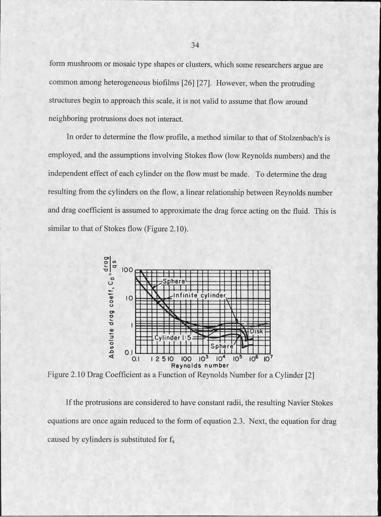
In order to determine the flow profile, a method similar to that of Stolzenbach's is
employed, and the assumptions involving Stokes flow (low Reynolds numbers) and the
independent effect of each cylinder on the flow must be made. To determine the drag
resulting from the cylinders on the flow, a linear relationship between Reynolds number
and drag coefficient is assumed to approximate the drag force acting on the fluid. This is
similar to that of Stokes flow (Figure 2.10).
Figure 2.10 Drag Coefficient as a Function of Reynolds Number for a Cylinder [2]
If the protrusions are considered to have constant radii, the resulting Navier Stokes
equations are once again reduced to the form of equation 2.3. Next, the equation for drag
caused by cylinders is substituted for fx
35
2.6Z
where p is fluid density, U is velocity as a function of y, A is the cross-section area of an
individual cylinder, Cd is the coefficient of drag (approximated as 12/Re) and N is the
number of cylinders per area. Substituting equation 2.6 into equation 2.3 and simplifying
leads to equation 2.7
d2U9 /
with
2.7
B = 6*vf*iVD
2.8
Here A and N ate previously defined, and D is the cylinder diameter. The solution to
equation 2.7, with the no slip-boundary condition at the substratum, and U=I at y=l,, was
determined analytically and is equation 2.9.
U I * e ~ B * y _|____ IeB —e B
B * y 2.9
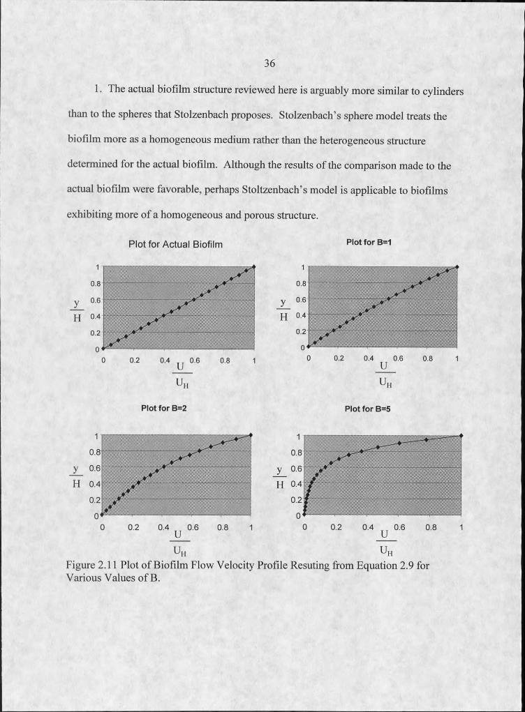
The results of equation 2.9 for various values of B are displayed graphically in
Figure 2.11. From these graphs, a profile similar to that provided by Stolzenbach's
model is seen, and the results here compare well with the results for the actual biofilm .
profile (Figure 2.11). Conclusions for comparison of this model is that it appears to have
the all the benefits of Stolzenbach5 s yet it is more realistic for the following reasons.
36
I . The actual biofilm structure reviewed here is arguably more similar to cylinders
than to the spheres that Stolzenbach proposes. Stolzenbach’s sphere model treats the
biofilm more as a homogeneous medium rather than the heterogeneous structure
determined for the actual biofilm. Although the results of the comparison made to the
actual biofilm were favorable, perhaps Stoltzenbach’s model is applicable to biofilms
exhibiting more of a homogeneous and porous structure.
Plot for Actual Biofilm Plot for B=1
Plot for B=2 Plot for B=S
1
0.8
y 0.6 H 0.4
0.2
0
* *
D 0.2 0.4 ^ 0.6 0.8
1
0.8
y 0.6
H 0.4
0.2
0
r"*.■
/ Sill:II I l0.4 ^ 0.6 0.8
u H u H
Figure 2.11 Plot of Biofilm Flow Velocity Profile Resuting from Equation 2.9 for Various Values of B.
37
2. The cylinder model could be further refined to more closely imitate actual
biofilm structure based on the changes in porosity at different heights within the biofilm.
For instance, to mimic the blunt colonies observed in many biofilms, the cylinders’ radii
could be assumed large at the base and then taper down away from the substratum. The
colonies could also be assumed to have small radii at the substratum and larger radii
within the canopy height. Such alterations would imitate the proposed mushroom model
[35].
Conclusion
Each of these methods can be used to estimate velocity profiles in biofilms that
have a highly porous heterogeneous structure. Unfortunately, this type of biofilm
structure is usually associated with biofilms grown under low flow velocities below those
relevant to industrial piping applications. Such industrial systems typically operate at
Reynolds numbers over 10,000 and fluid velocities on .the scale of meters per second
rather than centimeters per second. Therefore, a dramatically different approach is
needed to understand the problem of increased frictional losses in industrial biofouled
systems.
38
MATERIALS AND METHODS
. Introduction
In order to gain insight into the Mctional losses exhibited by biofouled systems,
several experiments were run. The purpose and results of the specific experiments are
included and discussed in Chapters 4 through 7. Although the specific objective of each
experiment varied, all the results were obtained from experiments that shared a similar
system, which consisted of a recycle loop containing a closed conduit reactor.
Throughout this reactor, biofilm growth and the corresponding pressure loss were
monitored. Rather than defining this system and its components in each of the following
chapters, the general system and method will be defined in this chapter and the details
specific to each experiment, which vary from the general layout, are included in the '
following chapters.
System Layout
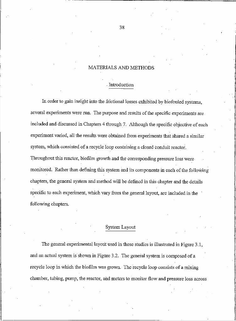
The general experimental layout used in these studies is illustrated in Figure 3.1,
and an actual system is shown in Figure 3.2. The general system is composed of a
recycle loop in which the biofilm was grown. The recycle loop consists of a mixing
chamber, tubing, pump, the reactor, and meters to monitor flow and pressure loss across
39
the reactor. The media, filtered air, and dilution water were added to the mixing chamber
that was vented to the atmosphere of the room. Flow through the recycle loop was
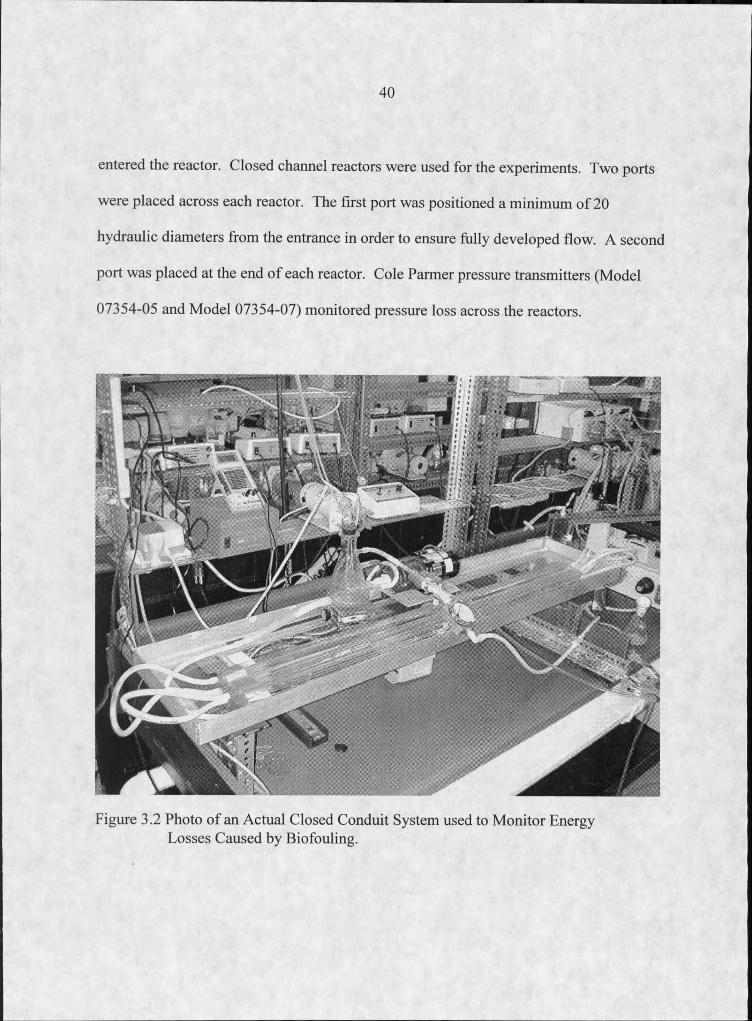
provided by either, a Cole Parmer pump (Model 7553-70) with an impeller pump head
attachment, or a Little Giant (Model 4-MD-HC) impeller pump (Figure 3.3). A pressure
vessel served as a pulse damper was placed after the pump in order to dampen flow
surges that may have been created by the pump. Down stream of the pulse damper, flow
MEDIA
Figure 3.1 The General System Layout used for the Experiments of Chapters 4 through 7
40
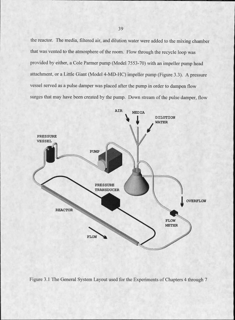
entered the reactor. Closed channel reactors were used for the experiments. Two ports
were placed across each reactor. The first port was positioned a minimum of 20
hydraulic diameters from the entrance in order to ensure fully developed flow. A second
port was placed at the end of each reactor. Cole Parmer pressure transmitters (Model
07354-05 and Model 07354-07) monitored pressure loss across the reactors.
Figure 3.2 Photo of an Actual Closed Conduit System used to Monitor Energy Losses Caused by Biofouling.
41
Growth Medium and Sterilization
The growth medium was the same for all experiments. The medium was diluted at
a twenty to one ratio with filtered tap water to a final concentration of 183 ppm
Na2HPO4, 35 ppm KH2P04, 19 ppm (NH4)2SO4, and 1.9 ppm MgSO4 * 7H20.
The reactors were sterilized by circulating a 5% bleach solution throughout for at
least 12 hours. The system was then flushed with filtered water until the pH returned to 7
and filled with media and dilution water. For the experiments involving 3 species, the
media and associated tubing were autoclaved for 2 hours at 121C in order to prevent
contamination. The media and dilution water were pumped to the system at a rate to
ensure a retention time of 20 to 30 minutes for all experiments.
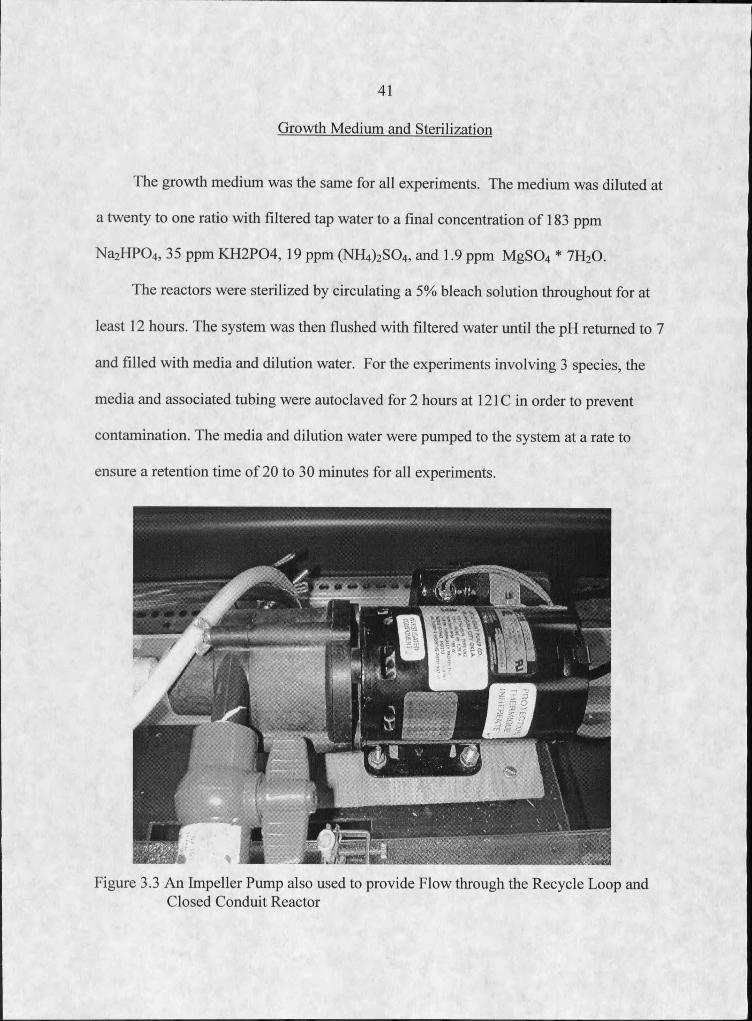
Figure 3.3 An Impeller Pump also used to provide Flow through the Recycle Loop and Closed Conduit Reactor
42
Bidfouling Method
The systems were inoculated with either a mixture of three species of bacteria
{Pseudomonas aeruginosa (ATCC 700829), Pseudamonas fluorescense (ATCC 700830),
and Klebsiellapneumoniea (ATCC 700831)) or activated sludge. For the experiments
involving the three species of bacteria, the media and associated tubing were autoclaved
for 2 hours at 121C in order to prevent contamination.
All systems once inoculated were run as a batch culture for 24 to 48 hours to ensure
microbial attachment. The systems were then switched to a continuous flow in order to
wash out all suspended microorganisms.
Growth media was delivered to a mixing chamber by peristaltic pumps and
recirculated within the system. Filtered air was bubbled into the mixing chamber to
provide oxygen. The growth media was diluted at a twenty to one ratio with filtered tap
water to a final concentration of 183 ppm Na2HPO4, 3.5 ppm KH2P04, 19 ppm
(NH4)2SO4, 1.9 ppm MgSO4 x 7H20, 40 ppm glucose and 10 ppm yeast extract. This
media and dilution water were pumped to the system at a rate to ensure a retention time
of 20 to 30 minutes for all experiments.
43
Measurement of Pressure Loss and Calculation of Friction Factors
Volumetric flow rates through the reactor were held constant throughout every
experiment and monitored using either a McMillan Co 101 Flo-Sen (Model 6593) or a
Great Plains Industries electronic flow meter (Model A104GMN025NA1) (Figures 3.4
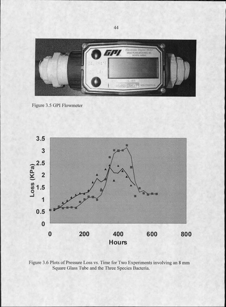
and 3.5). Pressure drop was recorded every 24 hours for each reactor. Figure 3.6 shows
graphically the data recorded from two of the experimental runs. From this graph, it is
also possible to see that the maximum frictional losses for these two experiments occur at
about 400 hours. Pressure across the reactors was monitored with Cole-Parmer pressure
transmitters (Model 07354-05 and Model 07354-07) (Figure 3.7) which were powered by
an Emco 24 Volt Power Supply (Figure 3.8). The transducers were calibrated using
water and a u-tube manometer. Friction factors were calculated by inserting the
parameters, V , fluid velocity, I , reactor length, and Ajy, the pressure loss, into the
Darcy-Weisbach equation (1.5) and solving for the friction factor.
Figure 3.4 Cole Parmer Flowmeter
44
Figure 3.5 GPI Flowmeter
Hours
Figure 3.6 Plots of Pressure Loss vs. Time for Two Experiments involving an 8 mm Square Glass Tube and the Three Species Bacteria.
45
Figure 3.7 A Cole Parmer Pressure Transducer
Figure 3.8 Emco 24 Volt Power Supply
46
CLOSED CONDUIT SYSTEM HEADLOSS AS A FUNCTION OF BIOFILM STRUCTURE
Introduction
Several researchers have suggested a connection between increased frictional losses
and filamentous biofilm morphology. Picologou et al. reported that "the filaments of the
biofilm flutter with a frequency that is a function of the average fluid velocity" and that
"frictional resistance increased with increasing filament length" [6], Lewkowicz and Das
attempted to simulate the filaments by adhering groups of fine nylon tufts to flat,,
hydraulically rough, plates that were then placed in a wind tunnel [23]. The plates
containing the filaments showed an 18% increase in frictional resistance over those
without the filaments. Schultz and Swain, who researched the effect of biofilms on
turbulent boundary layers using laser Doppler velocimetry, stated that "Waving algae
filaments seem to draw a greater amount of momentum from the flow than do slime films
alone" [24]. Stoodley and Lewandowski tracked the movement of a filament but were
unable to correlate the movement to any related frequency [15] [16]. Although all of
these observations do provide some insight into the problem of increased frictional
resistance associated with biofouling, they do not quantitatively relate biofilm structure to
energy losses associated with biofouling. The goal of this section, is to quantify a
relationship between biofilm filaments and increased frictional losses. To accomplish
47
this goal, two experiments were run. The first experiment was a porosity study, and is
explained in section 4.2. This experiment was performed in order to determine to what
extent the biofilm base acts as a constriction to a conduit diameter, i.e. while a highly
porous biofilm would have convective flow within it; a non-porous film would not. The
second was performed in order quantify a relationship between the filamentous biofilm
surface to the energy losses of the system.
Porosity Study
a) Porosity Study Materials and Method
The reactor system used for the porosity study was similar to the general
system layout of Figure 3.1. Because the method used to determine porosity
necessitated a reactor with favorable optical properties, a square borosilicate glass
tube (0.8 cm x 0.8 cm and 121 cm length, Freidrick & Douglas BST 800-80) was
used. Total system capacity was 450 ml. The system was inoculated with the 3
species of bacteria and run as a continuous culture with the medium described in
section 3.4. The three species biofilm was grown under a flow velocity of 0.81 m/s
and a Reynolds number of 6000. Porosity measurements were obtained by the
following method of biofilm imaging and image analysis.
48
b) Biofilm Imaging and Image Analysis
After 3 weeks of monitoring pressure loss and biofilm growth, I % v/v,
acridine orange (from Sigma) was added to the reactor to stain the three species
biofilm. The solution was recycled for 10 minutes to complete the staining
Following staining, confocal microscopy images were taken at 20 micron intervals
beginning at the biofilm/glass interface and then at every 20 microns through the
200 micron thick film and up to biofilm/fluid interface. The digital images of the
biofilm were takenin binary format. In these binary images, white (zero) is the area
void of biofilm while black (one) represents areas covered with biomass. The area
porosity is defined as the ratio of void area to total area. This calculation was
performed using the software Imagepro® (Media Cybernetics, Maryland).
c) Results of the Porosity Study
The graph shown in Figure 4.1 illustrates that the three species biofilm, grown
under initial non-fouled mean flow velocity of 0.81 m/s, had a dense base. This
observation agrees well with a close-up of the cross-sectioned image taken from the
second experiment that involved similar growth conditions and the vinyl tube
reactor (Figure 4.2). An isotropic view of a cross-section taken from this
experiment is shown in Figure 4.3. Because of the dense base and the relatively
small reactor sizes, for the remaining calculations and graphs, the biofilm base, as
shown in Figure 4.4, has been considered a constriction to the conduit. The
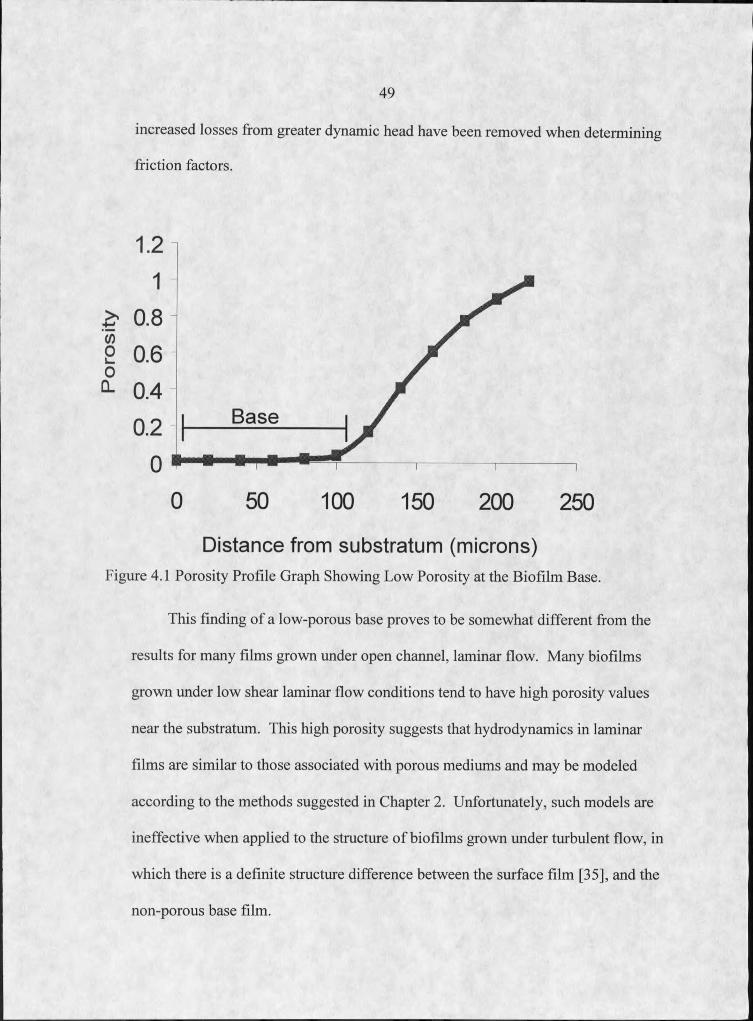
49
increased losses from greater dynamic head have been removed when determining
friction factors.
> 0.82 0.611 0.4
Base
0 50 100 150 200 250
Distance from substratum (microns)Figure 4.1 Porosity Profile Graph Showing Low Porosity at the Biofilm Base.
This finding of a low-porous base proves to be somewhat different from the
results for many films grown under open channel, laminar flow. Many biofilms
grown under low shear laminar flow conditions tend to have high porosity values
near the substratum. This high porosity suggests that hydrodynamics in laminar
films are similar to those associated with porous mediums and may be modeled
according to the methods suggested in Chapter 2. Unfortunately, such models are
ineffective when applied to the structure of biofilms grown under turbulent flow, in
which there is a definite structure difference between the surface film [35], and the
non-porous base film.
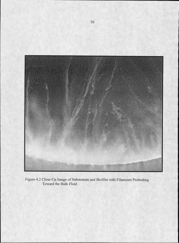
50
Figure 4.2 Close-Up Image of Substratum and Biofilm with Filaments Protruding Toward the Bulk Fluid
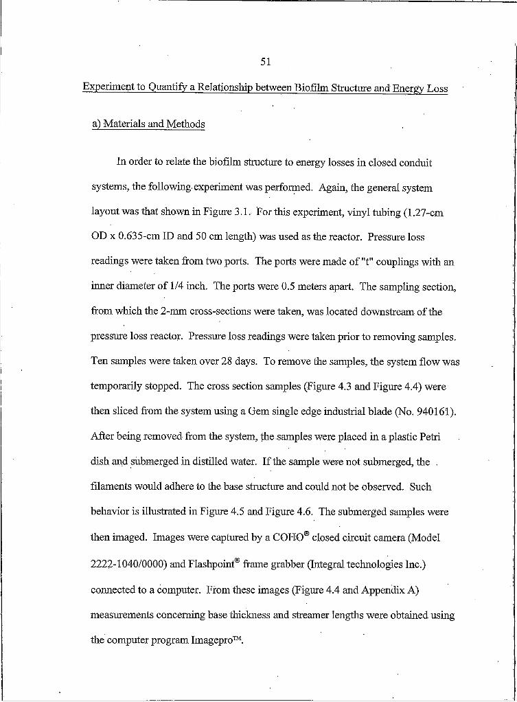
51
Experiment to Quantify a Relationship between Biofilm Structure and Energy Loss
a) Materials and Methods
In order to relate the biofilm structure to energy losses in closed conduit
systems, the following experiment was performed. Again, the general system
layout was that shown in Figure 3.1. For this experiment, vinyl tubing (1.27-cm
OD x 0.635-cm ID and 50 cm length) was used as the reactor. Pressure loss
readings were taken from two ports. The ports were made of "t" couplings with an
inner diameter of 1/4 inch. The ports were 0.5 meters apart. The sampling section,
from which the 2-mm cross-sections were taken, was located downstream of the
pressure loss reactor. Pressure loss readings were taken prior to removing samples.
Ten samples were taken over 28 days. To remove the samples, the system flow was
temporarily stopped. The cross section samples (Figure 4.3 and Figure 4.4) were
then sliced from the system using a Gem single edge industrial blade (No. 940161).
After being removed from the system, the samples were placed in a plastic Petri
dish and submerged in distilled water. If the sample were not submerged, the .
filaments would adhere to the base structure and could not be observed. Such
behavior is illustrated in Figure 4.5 and Figure 4.6. The submerged samples were
then imaged. Images were captured by a COHO® closed circuit camera (Model
2222-1040/0000) and Flashpoint® frame grabber (Integral technologies Inc.)
connected to a computer. From these images (Figure 4.4 and Appendix A)
measurements concerning base thickness and streamer lengths were obtained using
the computer program Imagepro™.
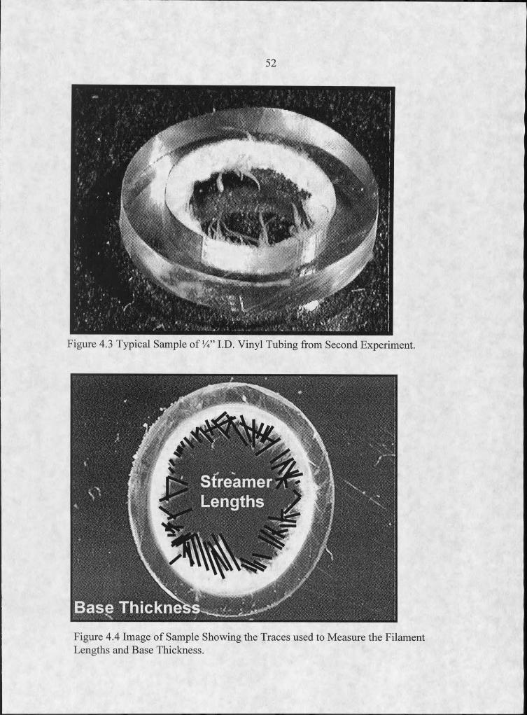
52
Figure 4.3 Typical Sample of 14” I D. Vinyl Tubing from Second Experiment.
Figure 4.4 Image of Sample Showing the Traces used to Measure the Filament Lengths and Base Thickness.
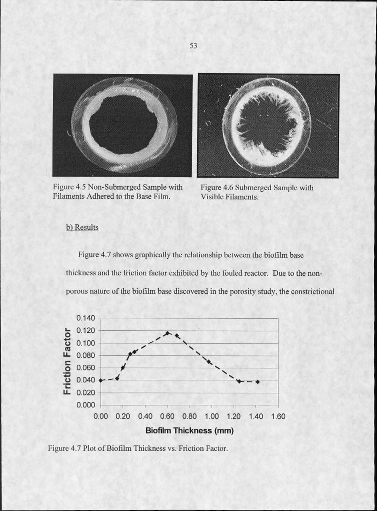
Fric
tion
Fact
or
53
Figure 4.5 Non-Submerged Sample with Figure 4.6 Submerged Sample with Filaments Adhered to the Base Film. Visible Filaments.
b) Results
Figure 4.7 shows graphically the relationship between the biofilm base
thickness and the friction factor exhibited by the fouled reactor. Due to the non-
porous nature of the biofilm base discovered in the porosity study, the constrictional
0.1400.120
0.100
0.0800.0600.0400.020
0.000
Biofilm T h ickn ess (m m )
Figure 4.7 Plot of Biofilm Thickness vs. Friction Factor.
54
effects have been incorporated into the calculation of the friction factor. This graph
shows that there is no direct relationship between biofilm thickness and frictional
losses.
In order to evaluate the effect of the filaments on pressure loss, the
Buckingham Pi Theorem [2] was applied using the traditional parameters: velocity,
hydraulic diameter, fluid density, viscosity, and reactor length. The roughness
element was replaced with the new parameter of total streamer length ( SI, ) per
effective volume (the effective volume resulting after considering the biofilm base
thickness a constriction to the tube diameter). This parameter is shown in equation
4.1. The motivation for choosing this parameter is included in the discussion.
M,.-------------- = 4.1
VoI-Jr
c) Dimensional Analysis
The dimensional analysis based on the parameter provided in 4,1 is as follows.
Step I . Establish the variables on which pressure loss is dependent.
Variable Representation
Ap - pressure loss across length of pipeV = mean fluid velocityDeff = Effective Diameter (Pipe Diameter less 2x the biofilm base thickness I = length of the pipep = dynamic viscosityp - fluid density
55
——---- Total streamer length per effective volume of cross section sample"olCif
Functional Fomi
SI
P h y
Dimensions
Use the primary dimensions of M (kg), L (m), ahd t (s).
Express Variables in Primary Dimensions
Apper length of pipe ->
I L■Dcjf , -> L
M 'Ii ->
L * tLV —>tM :
P ->■ L3
SI,->
IV°hff L2
Step 2. Choice of repeating variables V, Dejj, p
Step 3. Form dimensionless Pi groups based using these repeating variables.
System of equations evaluated for Ap.
A p * r * Ddr**/,'
A = M 0 * T0 * T'0
M I + 0 + 0 + c = 0 c = —l
56
L — 2 + <z + Z> + (—3c) = O 6 = 1
t — 2 + (—la) + 0 + 0 — 0 Ci = -L
System of equations evaluated for //
f0 * r0 * /-rrO
L *t t Z3
M l + 0 + 0 + c =0 C = - I
L — I + cz + 6 + (—3c) = 0 a = —I
t — I + (—a) + 0 + 0 = 0 A = - I
11I =:* Deff
n 2 =
Final system of equations be evaluated for SllK ff
SI,V„fe
I T a M c*z_ = M 0 *Z0 *!r0
r r Zj
M 0 + 0 + 0 + c =0 c = 0
L - 2 + a + b + (-3c) = 0 a = 0 simplifies Io fl3
t 0 + {-a) + 0 + 0 = 0 6 = 2
where Slj represents the crimulative,streamer length measured (per 2-mm sample),
and the denominator of this parameter is the volume of the cross section sample
thickness as shown in Figure 4.3. Measurement data is included in Appendix A.
This volume is calculated using the effective diameter i.e. the initial tube diameter
less 2 times the biofilm thickness. The final variable, I, is the length of the reactor.
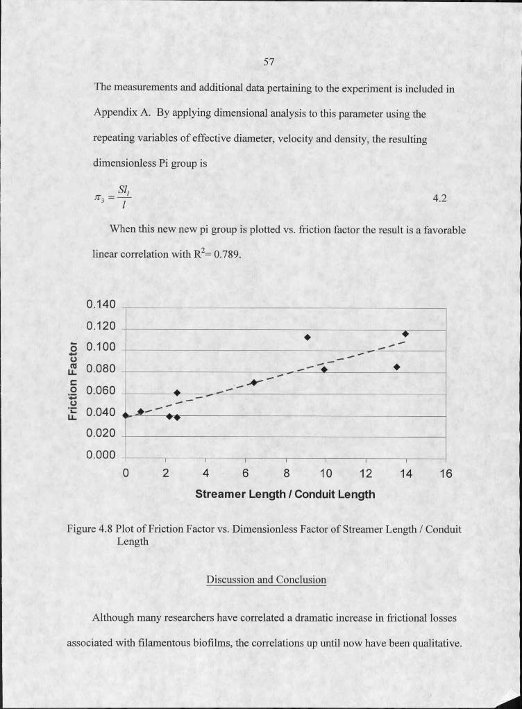
tio
n F
acto
r57
The measurements and additional data pertaining to the experiment is included in
Appendix A. By applying dimensional analysis to this parameter using the
repeating variables of effective diameter, velocity and density, the resulting
dimensionless Pi group is
SI,X3 = - j - 4.2
When this new new pi group is plotted vs. friction factor the result is a favorable
linear correlation with R2= 0.789.
0.140
0.120 0.100
0.080
0.060
^ 0.040
0.020
0.000
0 2 4 6 8 10 12 14 16
S tre a m e r L en g th / C onduit L en g th
Figure 4.8 Plot of Friction Factor vs. Dimensionless Factor of Streamer Length / Conduit Length
Discussion and Conclusion
Although many researchers have correlated a dramatic increase in frictional losses
associated with filamentous biofilms, the correlations up until now have been qualitative.
58.
Other investigators have indicated that attributed rippled biofilm topography, similar to
that shown in Figure 4.5, was responsible for the losses. Such observations may have
been the result of viewing the biofouled surface in a moist but not submerged state, i.e.
viewing a pipeline just after draining it out. Viewing the biofouled system in such
conditions the streamers would not be visible and could easily be overlooked.
These results are the first attempt to quantify a relationship between biofilm
structure and pressure loss associated with biofouling. Because natural systems are
complicated, much more so than a manufactured conduit surface, such an attempt is not
trivial and the following topics arise as points of discussion.
I . The replacement of the traditional roughness element (e / D) with the parameter
SI,in the dimensional analysis is not intuitively obvious as a parameter
based simply on the streamer length, but was selected over such a length
because of the following 2 reasons. .
a. This variable accounts for, not only the lengths of streamers, but also the
number (density) of streamers, i.e. this variable accounts for the total
streamer length per volume. By using a simple reference length based on
average streamer length ( Slave), the resulting Pi group, , would not
account for changes in the population of streamers.
59
b. Unlike the traditional roughness elements that perturb flow by protruding into
the flow, the streamers arguably lie parallel to the flow along the conduit wall.
iS7 SISuch a situation is better represented by the Pi group, ~ , rather than
c. It also should be noted that other possibilities exist for the variable such as
total streamer length per area of the conduit wall or streamer length squared
per area of the conduit wall.
2. The measuring technique was done carefully as described in the section 4.2.
Possible areas of uncertainty and the effects on the results are the following,
a. Variations in the thickness of the slice of tubing would be linearly related to a
change in the measurement of Sll•. For instance, a deviation in the length
eff
of the slice of 5% would be reflected in a 5% change in the recorded value of
SI,
'
b. The scale at which the measurements were performed on the images was
approximately 20 times. Changes in this scale could result in significant
changes in the measurements of the streamers. These differences would likely
be reflected in changes of measurements for all the images, but this would not
change the R2 value for the correlation in Figure 4.8.
3. Errors in the measurement of base thickness (Figure 4.4) of the biofilm would
be reflected in Calculations of the mean flow velocity in the reactor. Such errors
would be compounded when calculating the associated friction factor, due to the
60
velocity squared term in the Darcy equation. It is acknowledged that errors in
the thickness measurements may result in up to 15% error in the resulting
friction factor.
Despite these areas of uncertainty regarding the experiment, the results
nonetheless provide a fundamental quantitative relationship between biofilm structure
and pressure loss.
61
THE PHENOMENON OF INCREASING FRICTION FACTORS WITH INCREASING REYNOLDS NUMBERS IN BIOFOULED SYSTEMS.
Introduction
In the previous chapters, it was shown that traditional approaches fall short in
predicting losses in biofouled systems. Several industrial case studies where this
occurred were offered in Chapter I . Chapter 4 illustrated how the streamers lengths
found in some biofouled systems differ from the traditional parameter of the roughness
element, and in Chapter 4 the length of these filaments was related to the energy losses
through a dimensional analysis. In this chapter, another fundamental deviation from the
traditional losses caused by rigid roughness is investigated.
In a rigid, non-fouled conduit system, the frictional resistance and corresponding
friction factor are dependent on the two dimensionless parameters of roughness element
and Reynolds number. The relationship between these two parameters is predicted by the
Moody diagram and the Colebrook correlation for various roughnesses [2].. In addition,
the Blasius solution can be used to predict losses in hydraulically smooth conduits where
s ! D < 0.00005 [2], The Moody diagram applies to flow for all Reynolds numbers while
the Colebrook and Blasius solutions apply only to turbulent flows. For laminar flow the
value of the friction factor is independent of the surface and linearly related to the
Reynolds number [2],
62
To illustrate the general relationship between friction factor and Reynolds number,
consider a piping system of average diameter with the flow slowly increasing from the no
flow condition. Initially the flow velocity is low and the Reynolds number is less than
2,100, resulting in a laminar flow. As the flow velocity increases, the Reynolds number
increases and the friction factor falls off according to
This continues until the flow is increased to a point where the Reynolds number reaches
approximately 2100, and the friction factor is reduced to near 0.03. At this point, the
inertial force of the fluid becomes too high, relative to the viscosity, to maintain laminar
flow, and the flow enters a transitional zone. The transitional zone is characterized by
periods of laminar flow interrupted with bursts of turbulence. Here equation 5.1 becomes
ineffective at predicting the friction factor.
The nature of the flow in the transition zone creates a difficulty in predicting the
values of the friction factor with high degree accuracy. As the flow velocity is increased
to a point where the corresponding Reynolds number exceeds 4,000, the flow is fully
transitioned into turbulent flow. In this flow regime the values of the friction factor
become predictable again to within 5% to 10% using the Moody diagram and related
equations [2],
Unlike the laminar regime, friction factors related to turbulent flow are dependent
upon the roughness of the conduit wall. The Moody diagram provides friction factors for
a range the roughness elements varying from a !D < 0.00005 (hydraulically smooth) up
to 0.05.
63
The different relative roughnesses are represented on the Moody diagram by the set
of curves, all of which begin near a Reynolds number of 4,000. Similar curves can also .
be generated using the Colebrook equation (5.2) for the associated range of Reynolds
numbers and relative roughnesses [2].
V7= - 2.0 logr s !D 2.51 "
3.75.2
Where f is the friction factor, s ! D is the relative roughness and Re is the Reynolds
number. Because of the implicit dependence on the friction factor, f needs to be solved
for with an iterative method.
In addition, the Blasius equation (5.3) [2] can be used to predict losses for Reynolds
numbers in the range of 4,000 to 100,000 for smooth walled conduits.
D * ISpl p * V 2
0.1582 5.3
Where D is the hydraulic diameter, ISpl is the pressure loss, p is the fluid density, V is
the mean fluid velocity, and p is the dynamic viscosity of the fluid. The Blasius solution
is more tractable than the Colebrook solution but is limited to smooth wall conduits and
Reynolds numbers of the given range. Both the Colebrook and Blasius solutions are the
result of fitting an equation to numerous experimental results.
These methods show that for rigid wall pipes, friction factors in the turbulent
regime have their maximum value at Reynolds numbers representing the transition to
. fully turbulent flow. As Reynolds numbers increase from here, the friction factors
64
decrease in the manner shown on the Moody diagram and similarly represented
numerically by Colebrook and Blasius solution.
The goal of the following experimental was to show how friction factors exhibited
by biofouled closed conduits deviate from the aforementioned behavior. A discussion of
possible reasons for the deviation is then offered.
Materials and Methods Specific to Experiment
The general experimental setup is the same as that discussed in Chapter 3. 6.4-mm
inner diameter (9.5-mm outer diameter) clear vinyl tubing was used as the reactor. The
distance between the pressure ports was 0.5-m. Two Cole Parmer impeller pumps (Model
7553-70) placed in parallel provided the flow and a McMillan Co 101 Flo-Sen (Model
6593) measure the flow rate. The flow sensor was calibrated using tap water prior to the
experiment. The biofilm was grown under a volumetric flow rate of 41.9 ml/sec,
resulting in a flow velocity in the reactor of 1.3 m/s. The Reynolds number based on this
the diameter is approximately 7,500.
The reactor was inoculated with 250 ml of activated sludge that was obtained from
the Bozeman wastewater treatment facility, located on Springhill Road in Bozeman
Montana. This was reeirulated for 24 hours in the system with the medium described in
Chapter 3 to ensure attachment before switching to a continuous culture.
Pressure loss data for this experiment was obtained with a Cole-Parmer pressure
transmitter (Model 07354-05) that was calibrated, prior to the experiment, using water
and a u-tube manometer. Pressure readings for this experiment varied from the method
65
described in Chapter 3. For the purpose of this experiment, pressure readings were taken
over a large range of Reynolds numbers based upon the tube diameter and the bulk flow
velocity. Measurements were taken as the pumps and flow were incrementally increased
from a minimum to the maximum possible flow permitted by the pumps.
Results
Prior to fouling the system, pressure measurements were taken over the range of
Reynolds numbers permitted by the flows generated by the pumps. The resulting friction
factors were then compared to those predicted for laminar flow by 64/Re, and those
predicted for turbulent flow by the Blasius solution. The results are shown in Figure 5.1.
The comparison of the actual friction factor to the predicted is favorable in the laminar
flow regime at Reynolds numbers around .1000. Then, as the flow nears the transitional
zone the actual friction factor deviates from the 64/Re. This may be due to an early onset
of the transition zone caused by entrance conditions and/or the fact that the vinyl tube is
not truly a rigid surface. As the flow is increased to Reynolds numbers above 4,000 the
comparison of the friction factor to the Blasius solution is excellent and is numerically
expressed in Table 5.1.
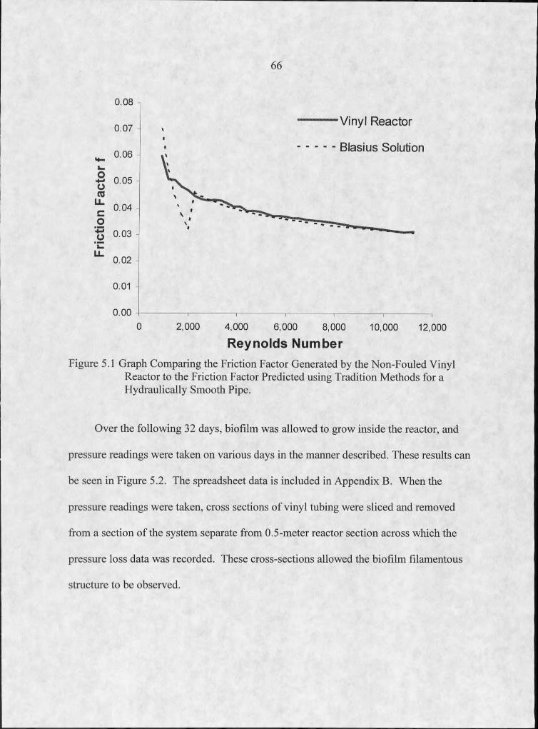
0.08
6 6
oro
LLCO4-»OLL
0.07
0.06
0.05
0.04
0.03
0.02
0.01
Vinyl Reactor
Blasius Solution
0.00 4------------------- —T------------------------------ T----------------------------T--------------------------- T----------------------------T--------------------------- ,
0 2,000 4,000 6,000 8,000 10,000 12,000
Reynolds NumberFigure 5.1 Graph Comparing the Friction Factor Generated by the Non-Fouled Vinyl
Reactor to the Friction Factor Predicted using Tradition Methods for a Hydraulically Smooth Pipe.
Over the following 32 days, biofilm was allowed to grow inside the reactor, and
pressure readings were taken on various days in the manner described. These results can
be seen in Figure 5.2. The spreadsheet data is included in Appendix B. When the
pressure readings were taken, cross sections of vinyl tubing were sliced and removed
from a section of the system separate from 0.5-meter reactor section across which the
pressure loss data was recorded. These cross-sections allowed the biofilm filamentous
structure to be observed.
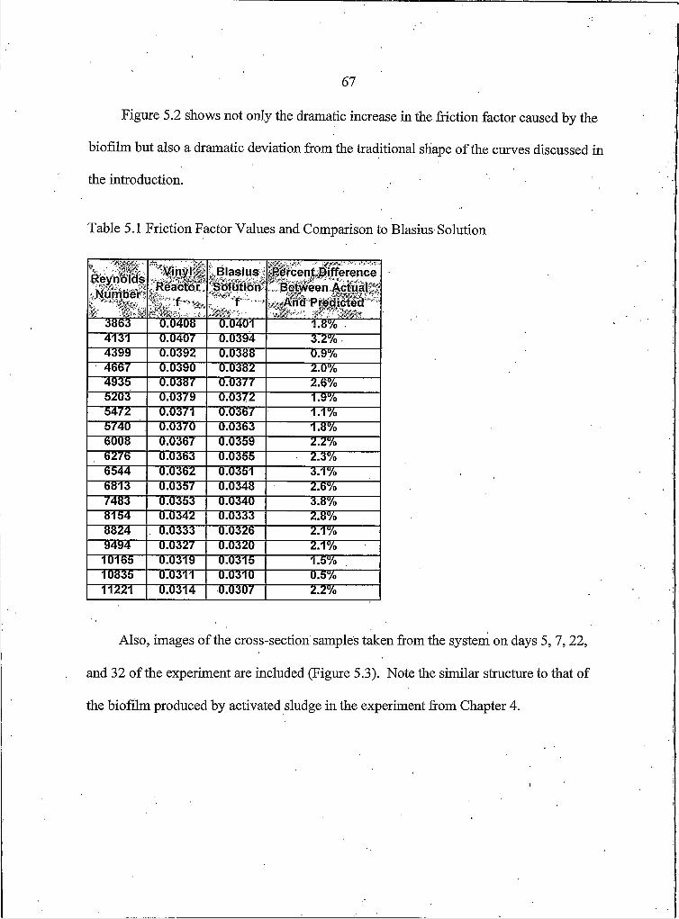
67
Figure 5.2 shows not only the dramatic increase in the friction factor caused by the
biofilm but also a dramatic deviation from the traditional shape of the curves discussed in
the introduction.
Table 5.1 Friction Factor Values and Comparison to Blasius Solution
# #B lasius
Sf s if3553 0.0408 0.0401 i . 8 % : “4131 0.0407 0.0394 3.2%4399 0.0392 0.0388 0l5%4667 0.0390 0.0382 2.0%4935 0.0387 0.0377 2.6%5203 0.0379 0.0372 1.9%5472 0.0371 0.0367 1.1%5740 0.0370 0.0363 1.8%6008 0.0367 0.0359 2.2%6276 0.0363 0.0355 2.3%6544 0.0362 0.0351 3.1%6813 0.0357 0.0348 2.6%7483 0.0353 0.0340 3.8%8154 0.0342 0.0333 2.8%8824 0.0333 0.0326 2.1%9494 0.0327 0.0320 2.1%
10165 0.0319 0.0315 1.5%10835 0.0311 0.0310 0.5%11221 0.0314 0.0307 2.2%
Also, images of the cross-section samples taken from the system on days 5, 7, 22,
and 32 of the experiment are included (Figure 5.3). Note the similar structure to that of
the biofilm produced by activated sludge in the experiment from Chapter 4.
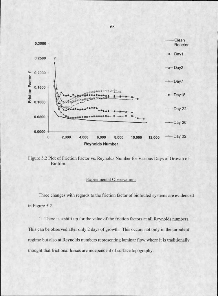
Fric
tion
Fact
or6 8
0.3000------Clean
Reactor
0.2500
0.2000
0.1500
0.1000
0.0500
Dayl
Day2
Day/
♦ -D a y 18
4— Day 22
— Day 26
0.0000 -------------- i--------------1--------------,--------------,--------------,--------------,0 2,000 4,000 6,000 8,000 10,000 12,000 Day 32
Reynolds Number
Figure 5.2 Plot of Friction Factor vs. Reynolds Number for Various Days of Growth of Biofilm.
Experimental Observations
Three changes with regards to the friction factor of biofouled systems are evidenced
in Figure 5.2.
I . There is a shift up for the value of the friction factors at all Reynolds numbers.
This can be observed after only 2 days of growth. This occurs not only in the turbulent
regime but also at Reynolds numbers representing laminar flow where it is traditionally
thought that frictional losses are independent of surface topography.
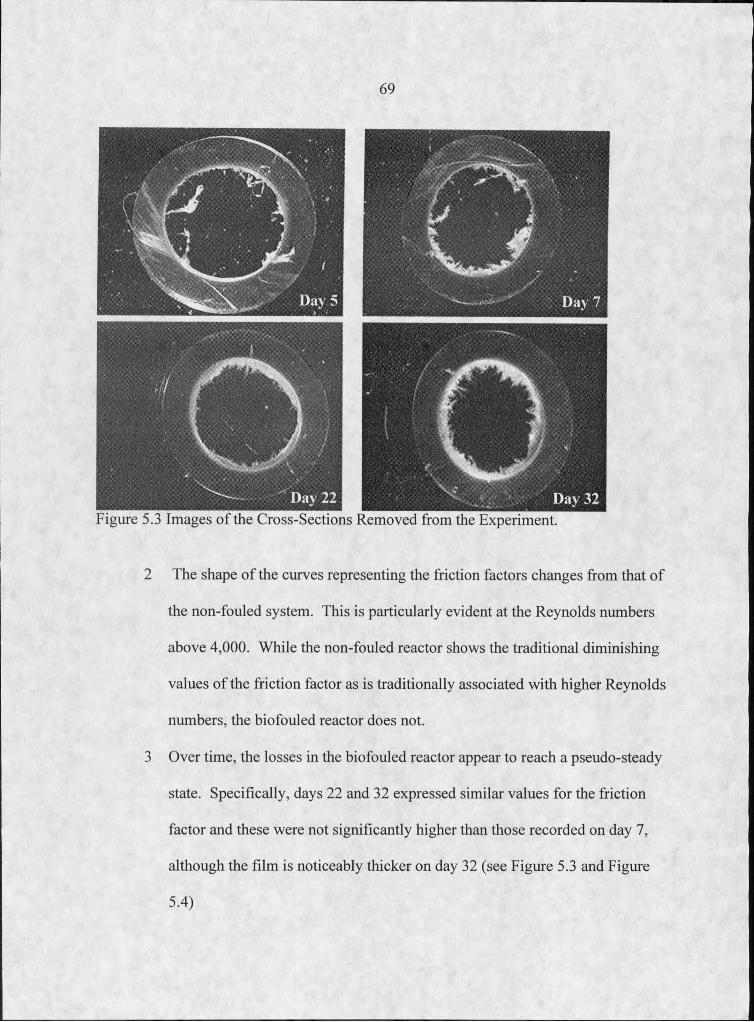
69
Figure 5.3 Images of the Cross-Sections Removed from the Experiment.
2 The shape of the curves representing the friction factors changes from that of
the non-fouled system. This is particularly evident at the Reynolds numbers
above 4,000. While the non-fouled reactor shows the traditional diminishing
values of the friction factor as is traditionally associated with higher Reynolds
numbers, the biofouled reactor does not.
3 Over time, the losses in the biofouled reactor appear to reach a pseudo-steady
state. Specifically, days 22 and 32 expressed similar values for the friction
factor and these were not significantly higher than those recorded on day 7,
although the film is noticeably thicker on day 32 (see Figure 5.3 and Figure
5.4)
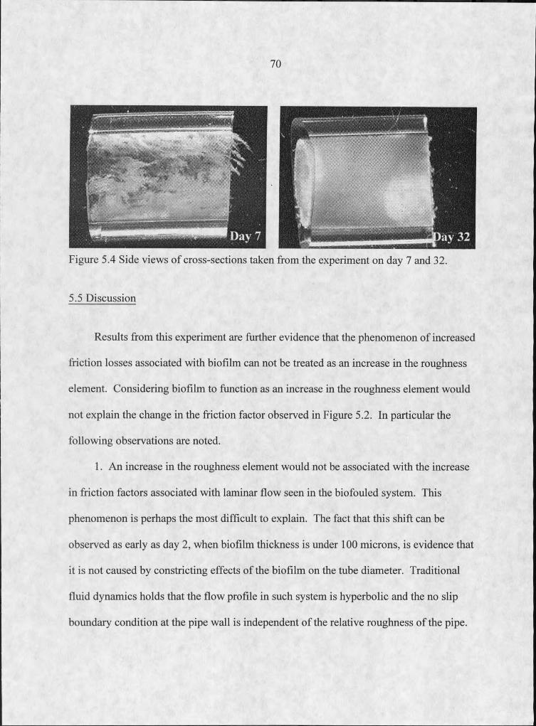
70
5.5 Discussion
Results from this experiment are further evidence that the phenomenon of increased
friction losses associated with biofilm can not be treated as an increase in the roughness
element. Considering biofilm to function as an increase in the roughness element would
not explain the change in the friction factor observed in Figure 5.2. In particular the
following observations are noted.
I . An increase in the roughness element would not be associated with the increase
in friction factors associated with laminar flow seen in the biofouled system. This
phenomenon is perhaps the most difficult to explain. The fact that this shift can be
observed as early as day 2, when biofilm thickness is under 100 microns, is evidence that
it is not caused by constricting effects of the biofilm on the tube diameter. Traditional
fluid dynamics holds that the flow profile in such system is hyperbolic and the no slip
boundary condition at the pipe wall is independent of the relative roughness of the pipe.
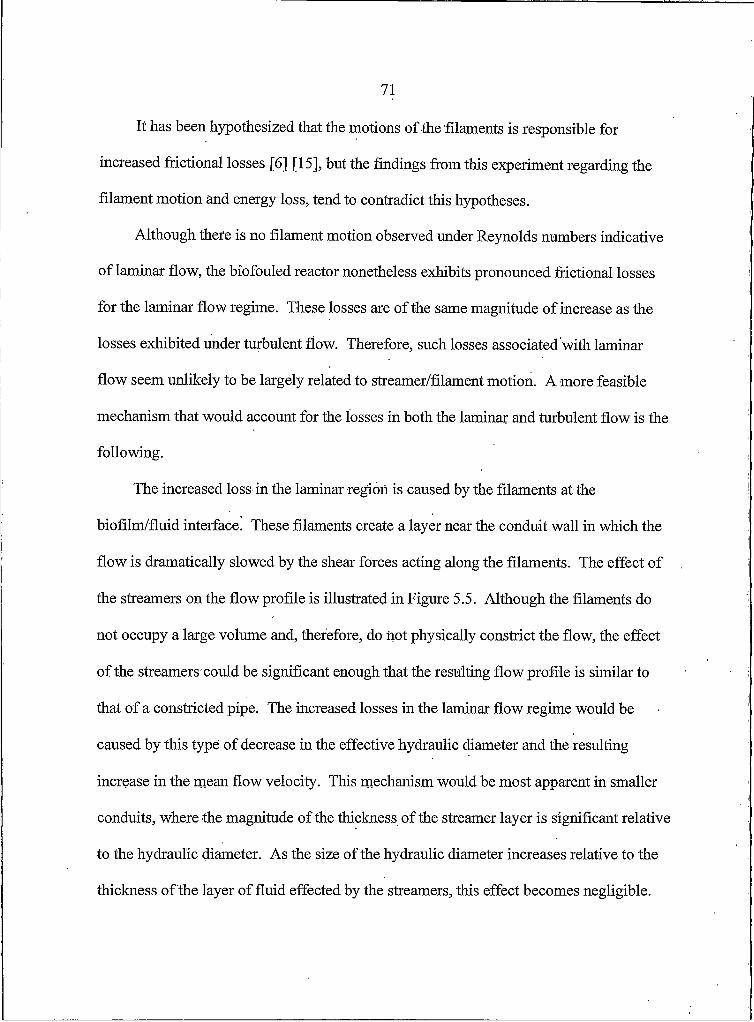
71
It has been hypothesized that the motions of the filaments is responsible for
increased frictional losses [6] [15], but the findings from this experiment regarding the
filament motion and energy loss, tend to contradict this hypotheses.
Although there is no filament motion observed under Reynolds numbers indicative
of laminar flow, the biofouled reactor nonetheless exhibits pronounced frictional losses
for the laminar flow regime. These losses are of the same magnitude of increase as the
losses exhibited under turbulent flow. Therefore, such losses associated with laminar
flow seem unlikely to be largely related to streamer/filament motion. A more feasible
mechanism that would account for the losses in both the laminar and turbulent flow is the
following.
The increased loss in the laminar region is caused by the filaments at the
biofilm/fluid interface. These filaments create a layer near the conduit wall in which the
flow is dramatically slowed by the shear forces acting along the filaments. The effect of
the streamers on the flow profile is illustrated in Figure 5.5. Although the filaments do
not occupy a large volume and, therefore, do not physically constrict the flow, the effect
of the streamers could be significant enough that the resulting flow profile is similar to
that of a constricted pipe. The increased losses in the laminar flow regime would be
caused by this type of decrease in the effective hydraulic diameter and the resulting
increase in the mean flow velocity. This mechanism would be most apparent in smaller
conduits, where the magnitude of the thickness of the streamer layer is significant relative
to the hydraulic diameter. As the size of the hydraulic diameter increases relative to the
thickness of the layer of fluid effected by the streamers, this effect becomes negligible.
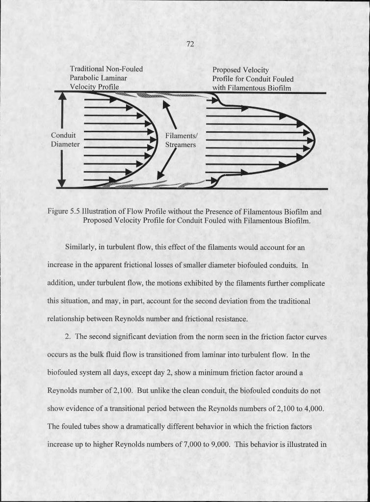
72
Traditional Non-Fouled Proposed VelocityParabolic Laminar Profile for Conduit FouledVelocity Profile with Filamentous Biofilm
ConduitDiameter
Filaments/Streamers
Figure 5.5 Illustration of Flow Profile without the Presence of Filamentous Biofilm and Proposed Velocity Profile for Conduit Fouled with Filamentous Biofilm.
Similarly, in turbulent flow, this effect of the filaments would account for an
increase in the apparent frictional losses of smaller diameter biofouled conduits. In
addition, under turbulent flow, the motions exhibited by the filaments further complicate
this situation, and may, in part, account for the second deviation from the traditional
relationship between Reynolds number and frictional resistance.
2. The second significant deviation from the norm seen in the friction factor curves
occurs as the bulk fluid flow is transitioned from laminar into turbulent flow. In the
biofouled system all days, except day 2, show a minimum friction factor around a
Reynolds number of 2,100. But unlike the clean conduit, the biofouled conduits do not
show evidence of a transitional period between the Reynolds numbers of 2,100 to 4,000.
The fouled tubes show a dramatically different behavior in which the friction factors
increase up to higher Reynolds numbers of 7,000 to 9,000. This behavior is illustrated in
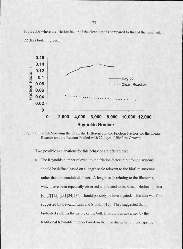
73
Figure 5.6 where the friction factor of the clean tube is compared to that of the tube with
22 days biofilm growth.
0.16 0.14
5 0.12 S 0.1c 0.08ip 0.06if 0.04
0.02 0
0
Day 22
Clean Reactor
I I I I I I
2,000 4,000 6,000 8,000 10,000 12,000Reynolds Number
Figure 5.6 Graph Showing the Dramatic Difference in the Friction Factors for the Clean Reactor and the Reactor Fouled with 22 days of Biofilm Growth.
Two possible explanations for this behavior are offered here,
a. The Reynolds number relevant to the friction factor in biofouled systems
should be defined based on a length scale relevant to the biofilm structure
rather than the conduit diameter. A length scale relating to the filaments,
which have been repeatedly observed and related to increased frictional losses
[6] [7] [15] [23] [24] [36], should possibly be investigated. This idea was first
suggested by Lewandowski and Stoodly [15]. They suggested that in
biofouled systems the nature of the bulk fluid flow is governed by the
traditional Reynolds number based on the tube diameter, but perhaps the
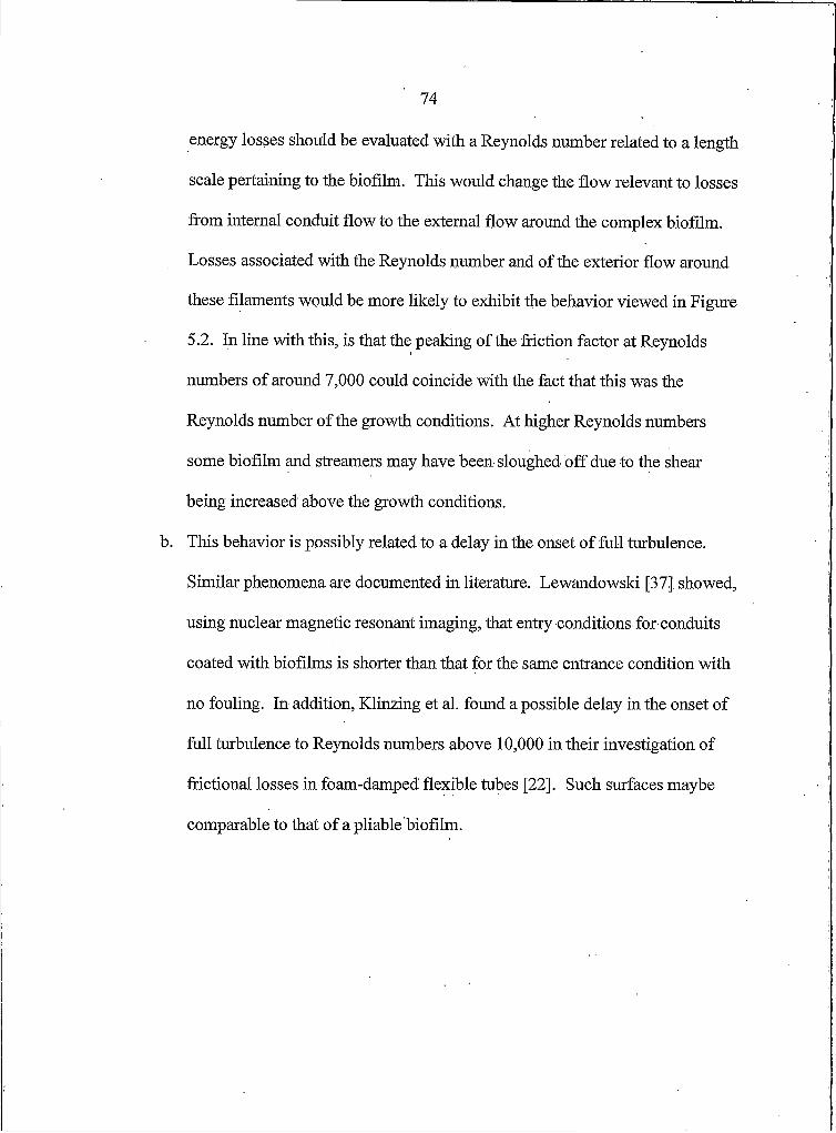
74
energy losses should be evaluated with a Reynolds number related to a length
scale pertaining to the biofilm. This would change the flow relevant to losses
from internal conduit flow to the external flow around the complex biofilm.
Losses associated with the Reynolds number and of the exterior flow around
these filaments would be more likely to exhibit the behavior viewed in Figure
5.2. In line with this, is that the peaking of the friction factor at Reynolds
numbers of around 7,000 could coincide with the fact that this was the
Reynolds number of the growth conditions. At higher Reynolds numbers
some biofilm and streamers may have been sloughed off due to the shear
being increased above the growth conditions,
b. This behavior is possibly related to a delay in the onset of full turbulence.
Similar phenomena are documented in literature. Lewandowski [37] showed,
using nuclear magnetic resonant imaging, that entry conditions for conduits
coated with biofilms is shorter than that for the same entrance condition with
no fouling. In addition, Klinzing et al. found a possible delay in the onset of
full turbulence to Reynolds numbers above 10,000 in their investigation of
frictional losses in foam-damped flexible tubes [22]. Such surfaces maybe
comparable to that of a pliable biofilm.
75
Conclusions
1. The filamentous biofilm structure increases frictional resistance in closed
conduits.
2. There are several ways that the increased frictional resistance is not consistent
with an increase in the roughness element.
o Increased losses under laminar conduit flow,
o Friction factor behavior is not consistent within the traditional
transition between laminar and turbulent flow,
o Friction factor behavior at Reynolds numbers between 4,000 and 8,000
increases rather than decreases.
3. A possible explanation for the dramatic increase in losses in relatively small
diameter conduits is that the streamers dramatically slow flow in a region near
the conduit wall.
76
SIMULATING A FILAMENTOUS BIOFILM SURFACE
Introduction
Chapter 5 showed that the filamentous biofilm surface topography is related to
increased frictional losses and Chapter 6 illustrated how these losses deviate
dramatically from those of rigid wall conduits. The goal of the experiment of this
chapter was to simulate the frictional resistance exhibited by the filamentous biofilms
of the experiments presented in Chapter 5 and Chapter 6. In order to simulate a
biofouled conduit, a pipe was lined with filamentous material, subjected to flow, and
the resulting frictional resistance was recorded and compared to the frictional
resistance exhibited by biofouled systems.
Materials and Methods
Acrylic fur, acquired from a local material store, was used to simulate the
fluid/filamentous interface exhibited by some biofilms. Prior to applying the acrylic
fur to the inside of the pipe, the fur was sheared to a shorter length to simulate the
topography discussed in chapter 4. The acrylic fur was then mounted to the inside of
a closed conduit in the following way.
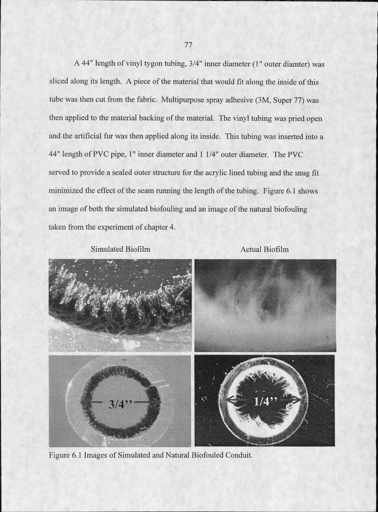
77
A 44" length of vinyl tygon tubing, 3/4" inner diameter (I" outer diamter) was
sliced along its length. A piece of the material that would fit along the inside of this
tube was then cut from the fabric. Multipurpose spray adhesive (3M, Super 77) was
then applied to the material backing of the material. The vinyl tubing was pried open
and the artificial fur was then applied along its inside. This tubing was inserted into a
44" length of PVC pipe, I" inner diameter and I 1/4" outer diameter. The PVC
served to provide a sealed outer structure for the acrylic lined tubing and the snug fit
minimized the effect of the seam running the length of the tubing. Figure 6.1 shows
an image of both the simulated biofouling and an image of the natural biofouling
taken from the experiment of chapter 4.
Simulated Biofilm Actual Biofilm
Figure 6.1 Images of Simulated and Natural Biofouled Conduit.
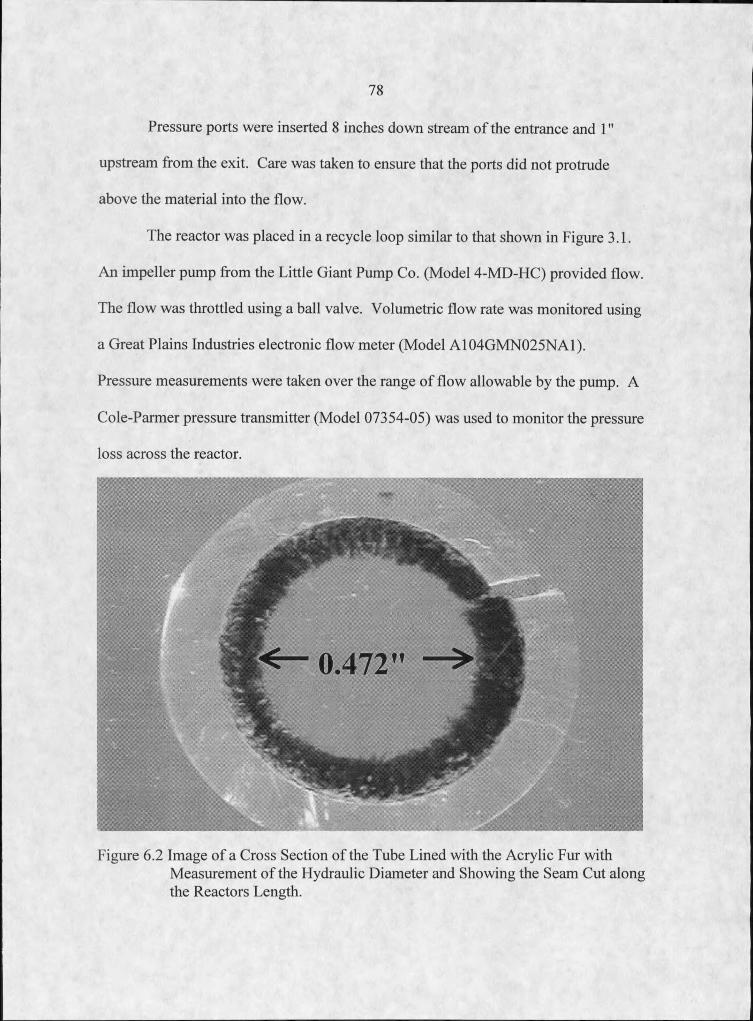
78
Pressure ports were inserted 8 inches down stream of the entrance and I"
upstream from the exit. Care was taken to ensure that the ports did not protrude
above the material into the flow.
The reactor was placed in a recycle loop similar to that shown in Figure 3.1.
An impeller pump from the Little Giant Pump Co. (Model 4-MD-HC) provided flow.
The flow was throttled using a ball valve. Volumetric flow rate was monitored using
a Great Plains Industries electronic flow meter (Model A104GMN025NA1).
Pressure measurements were taken over the range of flow allowable by the pump. A
Cole-Parmer pressure transmitter (Model 07354-05) was used to monitor the pressure
loss across the reactor.
Figure 6.2 Image of a Cross Section of the Tube Lined with the Acrylic Fur withMeasurement of the Hydraulic Diameter and Showing the Seam Cut along the Reactors Length.
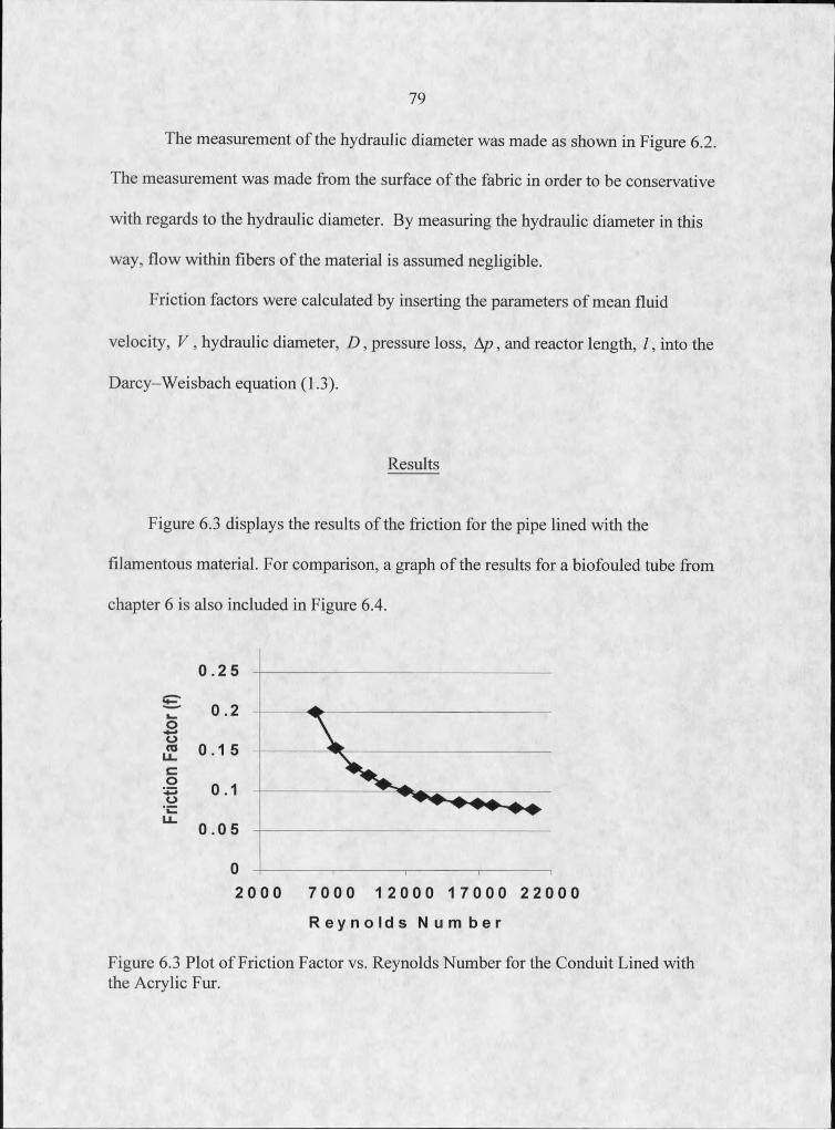
79
Fhe measurement of the hydraulic diameter was made as shown in Figure 6.2.
The measurement was made from the surface of the fabric in order to be conservative
with regards to the hydraulic diameter. By measuring the hydraulic diameter in this
way, flow within fibers of the material is assumed negligible.
Friction factors were calculated by inserting the parameters of mean fluid
velocity, V , hydraulic diameter, D , pressure loss, Ap, and reactor length, I , into the
Darcy-Weisbach equation (1.3).
Results
Figure 6.3 displays the results of the friction for the pipe lined with the
filamentous material. For comparison, a graph of the results for a biofouled tube from
chapter 6 is also included in Figure 6.4.
0 . 2 5
0 . 0 5
2 0 0 0 7 0 0 0 1 2 0 0 0 1 7 0 0 0 2 2 0 0 0
R e y n o l d s N u m b e r
Figure 6.3 Plot of Friction Factor vs. Reynolds Number for the Conduit Lined with the Acrylic Fur.
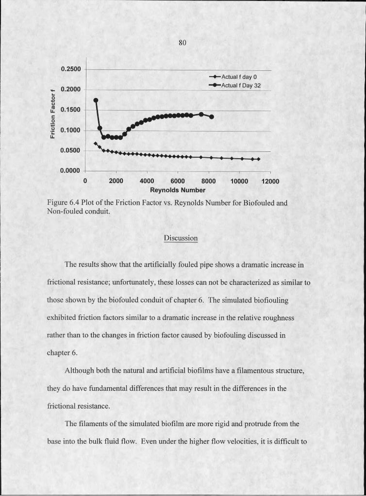
8 0
0.2500Actual f day 0 ■Actual f Day 320.2000
0.1500
0.1000
0.0500
0.00002000 IO 6000 8<
Reynolds Number10000 12000
Figure 6.4 Plot of the Friction Factor vs. Reynolds Number for Biofouled and Non-fouled conduit.
Discussion
The results show that the artificially fouled pipe shows a dramatic increase in
frictional resistance; unfortunately, these losses can not be characterized as similar to
those shown by the biofouled conduit of chapter 6. The simulated biofiouling
exhibited friction factors similar to a dramatic increase in the relative roughness
rather than to the changes in friction factor caused by biofouling discussed in
chapter 6.
Although both the natural and artificial biofilms have a filamentous structure,
they do have fundamental differences that may result in the differences in the
frictional resistance.
The filaments of the simulated biofilm are more rigid and protrude from the
base into the bulk fluid flow. Even under the higher flow velocities, it is difficult to
81
imagine that the filaments of the simulated film flex or yield much to. the flow. It
would follow that the simulated surface would exhibit frictional resistance more
closely related to a rough rigid surface rather than that of the pliable filamentous
biofilm.
Increased frictional resistance in the simulated system would be attributed
primarily to the pressure drag as the filaments function as cylinders in a cross flow.
Where as the filaments in the biofouled system would more accurately be represented
as cylinders parallel to the flow, in which shear rather than pressure is the primary
mechanism of frictional resistance.
82
A RELATIONSHIP BETWEEN MEAN FLOW VELOCITY AND FRICTION FACTORS EXHIBITED BY BIOFOULED SYSTEMS
Introduction
Chapters 4 through 6 investigated several aspects of the relationship between
biofilm structure and fluid flow. Chapter 7 investigated an attempt to simulate these
losses by artificially simulating the biofilm fluid interface in a closed conduit. Many
insights into the problem of increased friction factor were gained through these
experiments but such information and knowledge cannot easily be applied to industrial
applications.
This chapter looks at the results gathered from these experiments and others, and
shows that frictional losses in biofouled closed conduit systems are more dependent on
the fluid flow velocity arid less dependent on the Reynolds number.
System Layout and Reactors
Twelve experiments were conducted. All shared a layout similar to (Figure 3.1).
The experiments were all run with the media described in Chapter 3 except for four
experiments that used the same buffer but had 240 ppm glucose. Closed channel reactors
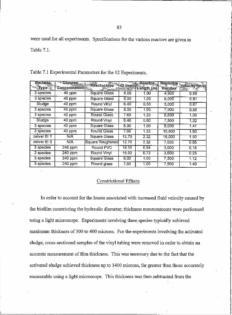
83
were used for all experiments. Specifications for the various reactors are given in
Table 7.1.
Table 7.1 Experimental Parameters for the 12 Experiments.
10 |mm-3 species ■ 40 ppm Square Glass 8.00 1.00 4,900 0.693 species 40 ppm Square Glass 8.00 1.00 6,000 0.81Sludge 40 ppm Round Vinyl 6.40 0.50 5,000 0.87
3 species 40 ppm Square Glass 8.00 1.00 7,000 0.983 species 40 ppm Round Glass 7.60 1,22 6,800 1,00Sludge 40 ppm Round Vinyl 6.40 0.50 7,500 1.32
3 species 40 ppm Square Glass 6.00 . 1.00 8,000 1.413 species 40 ppm Round Glass 7.60 1.22 10,800 1.60
zelver tfr 1 N/A Square Glass 12.70 2.32 16,000 1.50zelver tfr 3 N/A Square Roughened 12.70 2.32 7,000 0.653 species 240 ppm Round PVC 19.10 0.94 3,000 0.183 species 240 ppm Round Vinyl 15.90 0.73 3,600 0.253 species 240 ppm Square Glass 6.00 1.00 7,500 1.123 species 240 ppm Round glass 7.60 1.00 7,500 1.40
Constrictional Effects
In order to account for the losses associated with increased fluid velocity caused by
the biofilm constricting the hydraulic diameter; thickness measurements were performed
using a light microscope. Experiments involving three species typically achieved
maximum thickness of 300 to 400 microns. For the experiments involving the activated
sludge, cross-sectioned samples of the vinyl tubing were removed in order to obtain an
accurate measurement of film thickness. This was necessary due to the fact that the
activated sludge achieved thickness up to 1400 microns, far greater than those accurately
measurable using a light microscope. This thickness was then subtracted from the
84
reactors hydraulic diameter when calculating the mean fluid velocity from the volumetric
flow rate. Figures 4.3 and 4.4 show one of these cross-sections from which thickness
measurements were made for the activated sludge.
Results
Prior to fouling, the 12 reactors produced frictional resistance within 5% of values
predicted by the Blasius equation and the Moody diagram. As the reactors became
fouled with biofilm, there were dramatic increases in the frictional resistance. This
increase peaked at a maximum before falling off due to a change in biofilm structure or
sloughing of the film from the conduit wall. The maximum frictional losses correspond
to friction factors ranging from 0.05 to 0.24. The resulting maximum friction factors
from each experiment are provided in Table 7.2.
In Figure 7.1, the maximum friction factor recorded for each of the 12 experiments
are plotted vs. the Reynolds number. These points are then fit with a linear regression
and the resulting R2 value is 0.5175.
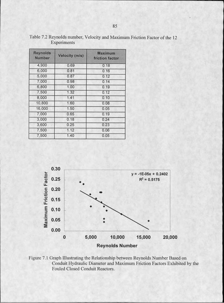
85
Table 7.2 Reynolds number, Velocity and Maximum Friction Factor of the 12 Experiments
ReynoldsNumber Velocity (m/s) Maximum
friction factor
4,900 0.69 0.186,000 0.81 0.165,000 0.87 0.127,000 0.98 0.146,800 1.00 0.197,500 1.32 0.128,000 1.41 0.1010,800 1.60 0.0816,000 1.50 0.057,000 0.65 0.193,000 0.18 0.243,600 0.25 0.237,500 1.12 0.067,500 1.40 0.05
0.30L -Oo 0.25(9
= 0.20♦3
c 0.15U-
| 0.10 Ex 0 .05COS
0.000 5 ,000 10 ,000 15,000 20 ,000
R eyn o ld s N u m b er
Figure 7.1 Graph Illustrating the Relationship between Reynolds Number Based onConduit Hydraulic Diameter and Maximum Friction Factors Exhibited by the Fouled Closed Conduit Reactors.
y = -1 E-OSx + 0.2402 R2 = 0.5175
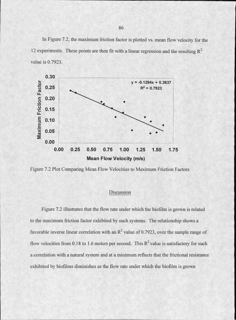
86
In Figure 7.2, the maximum friction factor is plotted vs. mean flow velocity for the
12 experiments. These points are then fit with a linear regression and the resulting R2
value is 0.7923.
y = -0.1294x + 0.2637 R2 = 0.7923O 0.25
c 0.20
c 0.15
S 0.05
0.00 0.25 0.50 0.75 1.00 1.25 1.50
M ean F lo w V e loc ity (m /s)
Figure 7.2 Plot Comparing Mean Flow Velocities to Maximum Friction Factors
Discussion
Figure 7.2 illustrates that the flow rate under which the biofilm is grown is related
to the maximum friction factor exhibited by such systems. The relationship shows a
favorable inverse linear correlation with an R2 value of 0.7923, over the sample range of
flow velocities from 0.18 to 1.6 meters per second. This R2 value is satisfactory for such
a correlation with a natural system and at a minimum reflects that the frictional resistance
exhibited by biofilms diminishes as the flow rate under which the biofilm is grown
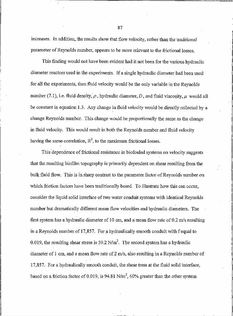
87
increases. In addition, the results show that flow velocity, rather than the traditional
parameter of Reynolds number, appears to be more relevant to the frictional losses.
This finding would not have been evident had it not been for the various hydraulic
diameter reactors used in the experiments. If a single hydraulic diameter had been used
for all the experiments, then fluid velocity would be the only variable in the Reynolds
number (7.1), i.e. fluid density, p , hydraulic diameter, D , and fluid viscosity, /u would all
be constant in equation 1.3. Any change in fluid velocity would be directly reflected by a
change Reynolds number. This change would be proportionally the same as the change
in fluid velocity. This would result in both the Reynolds number and fluid velocity
having the same correlation, R2, to the maximum frictional losses.
This dependence of frictional resistance in biofouled systems on velocity suggests
that the resulting biofilm topography is primarily dependent on shear resulting from the
bulk fluid flow. This is in sharp contrast to the parameter factor of Reynolds number on
which friction factors have been traditionally based. To illustrate how this can occur,
consider the liquid solid interface of two water conduit systems with identical Reynolds
number but dramatically different mean flow velocities and hydraulic diameters. The
first system has a hydraulic diameter of 10 cm, and a mean flow rate of 0.2 m/s resulting
in a Reynolds number of 17,857. For a hydraulically smooth conduit with f equal to
0.019, the resulting shear stress is 59.2 N/m2. The second system has a hydraulic
diameter of I cm, and a mean flow rate of 2 m/s, also resulting in a Reynolds number of
17,857. For a hydraulically smooth conduit, the shear tress at the fluid solid interface,
based on a friction factor of 0.019, is 94.81 N/m2, 60% greater than the other system
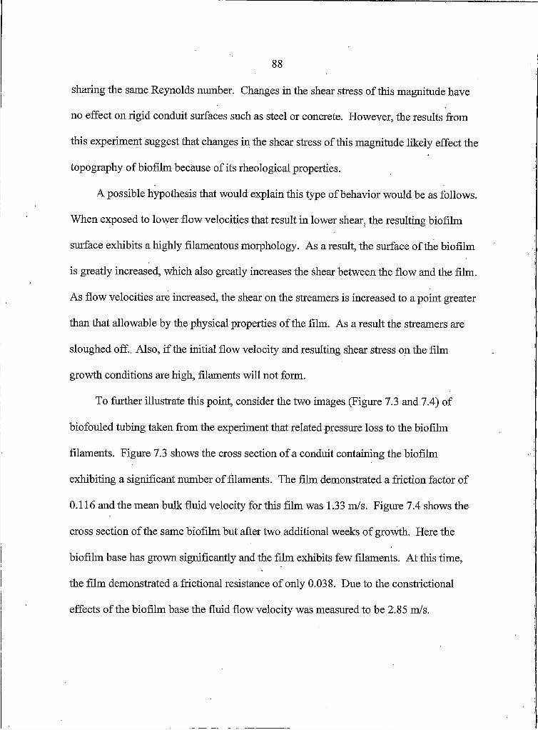
88
sharing the same Reynolds number. Changes in the shear stress of this magnitude have
no effect on rigid conduit surfaces such as steel or concrete. However, the results from
this experiment suggest that changes in the shear stress of this magnitude likely effect the
topography of biofilm because of its rheological properties.
A possible hypothesis that would explain this type of behavior would be as follows.
When exposed to lower flow velocities that result in lower shear, the resulting biofilm
surface exhibits a highly filamentous morphology. As a result, the surface of the biofilm
is greatly increased, which also greatly increases the shear between the flow and the film.
As flow velocities are increased, the shear on the streamers is increased to a point greater
than that allowable by the physical properties of the film. As a result the streamers are
sloughed off. Also, if the initial flow velocity and resulting shear stress on the film
growth conditions are high, filaments will not form.
To further illustrate this point, consider the two images (Figure 7.3 and 7.4) of
biofouled tubing taken from the experiment that related pressure loss to the b i o f i lm
filaments. Figure 7.3 shows the cross section of a conduit containing the biofilm
exhibiting a significant number of filaments. The film demonstrated a friction factor of
0.116 and the mean bulk fluid velocity for this film was 1.33 m/s. Figure 7.4 shows the
cross section of the same biofilm but after two additional weeks of growth. Here the
biofilm base has grown significantly and the film exhibits few filaments. At this time,
the film demonstrated a frictional resistance of only 0.038. Due to the constrictional
effects of the biofilm base the fluid flow velocity was measured to be 2.85 m/s.
89
Figure 7.3 Biofilm Structure for Figure 7.4 Biofilm Structure forBulk Fluid Velocity of 1.33 m/s. Bulk Fluid velocity of 2.85.
This calculation was based on the volumetric flow rate and the constricted tube diameter
caused by the biofilm base thickness. At this high flow velocity the frictional resistance
created at the biofilm surface is approximately equivalent to that of a hydraulically
smooth surface.
Conclusion
The relationship between flow velocity and frictional resistance has implications for
both the practicing engineer and those further researching this problem.
For the practicing engineer who is designing hydraulic pipelines prone to
biofouling, these results demonstrate that the effects of increased pressure losses due to
biofouling will be minimized if the system is operated at higher flow velocities. If this is
not feasible then the engineer must anticipate the possibility of large frictional resistance
and incorporate additional costs of reduction in flow and treatment measures into design
analysis. Figure 7.2 may be used to conservatively estimate the maximum possible
friction losses in such systems.
• Implications involving further research suggest flow velocity or more specifically,
shear stress, plays a more important role than the traditional parameter of Reynolds
Number with respect to losses in biofouled systems.
90
91
CONCLUSION AND FUTURE WORK
For past researchers, determining a method of predicting frictional losses in closed
conduits was not trivial. To this day, methods such as the Colebrook equation, Blasius
equation and the Moody diagram which are used to predict losses in clean, new conduits,
are methods empirically based on tens of thousands of experiments. Predicting losses in
systems where the manufactured fluid-solid interface of a pipe wall has become covered
with the complex topography of a compliant biofilm is an even more daunting task. The
biofilm greatly complicates an already difficult problem. The research presented in this
thesis provides a further understanding of the problem of increased frictional resistance
associated with biofouled conduits.
In Chapter 2, it was shown that for relatively slow flows in porous biofilms,
velocity profiles can be modeled using flow profiles of a vegetative canopy, or, if enough
assumptions are made, using simple canopy models and the Navier Stokes equations.
Such methods are simplified approaches to a complicated problem, but nonetheless,
resulting profiles generated by these approaches satisfactorily compared to a flow profile
acquired from an actual biofilm. Therefore these methods may be used to estimate flow
profiles in highly porous heterogeneous biofilms.
Unfortunately, for biofilms grown under higher turbulent flow rates in closed
conduits, the situation is further complicated. As shown in Chapter 4, these biofilms
have a non-porous base from which filaments protrude. These filaments exhibit
92
movements as they interact with the turbulent flow. For these filamentous biofilms,
many past researchers have suggested that there is a correlation between the filaments
and the increased frictional losses exhibited by the system. Here in Chapter 4, for the
first time, an experiment was performed which measured the lengths of the streamers and
quantified, using dimensional analysis, a relationship between the lengths of these
filaments and the frictional losses in closed conduits.
Next, in Chapter 5, it was shown that rather than simply increasing frictional losses
in a manner similar to that of an increase in rigid roughness, losses due to biofouling
deviate from losses caused by rigid roughness in the following ways.
1. The biofouled systems exhibited increased losses in the laminar regime.
Traditionally, pressure losses for laminar flows are independent of the interface
topography. The cause of this increase was attributed to the filaments
sufficiently slowing the flow near the interface, i.e. the filaments act as a
pseudo-constriction to the flow. This effect is likely magnified due to the
relatively small scale of the laboratory experiments.
2. Although the friction factors of biofouled systems appear to show a transition
from laminar to transitional flow at Reynolds numbers near 2,100, the friction
factors were not indicative of the transition to full turbulence at a Reynolds
numbers near 4,000
3. Unlike rigid conduits in which friction factors decrease as flow becomes more
turbulent, friction factors in the biofouled systems increased well into the

93
turbulent regime. This increase was possibly attributed to movements of the
streamers and biofilm in response to the bulk fluid flow.
In order to verify that the filaments caused these deviations from the traditional
frictional losses, a simulation of the filamentous interface was attempted. Unfortunately,
the attempt was unsuccessful. The failure was attributed to the fact that the filaments of
the material used to simulate the biofilm were sufficiently stiff to protrude into the flow
rather than lie parallel to the flow as the pliable biofilm filaments were observed to do.
Future attempts to simulate the filamentous interface should focus on finding or
manufacturing a material that more accurately simulates the biofilm filaments, but
obtaining such a material most likely will not be easy.
Finally, in Chapter 7 the results of all the experiments were revisited to find that the
velocity is a more influential factor than Reynolds number on the biofilm structure and
therefore its ability to greatly increase frictional losses. Possible future work could
further verify this by growing biofilms under constant Reynolds numbers, but with
varying velocities.
In order to gain a better understanding of this complex problem, future work
investigating the increased frictional losses associated with biofouling should take a step
back from closed conduits and focus on the shear force exhibited on biofouled flat plate
(or rotating disk) reactors. By utilizing these open channel reactors, future research
would take a simplified approach to the problem by avoiding several of the problems and
pitfalls implicit to the closed conduit flow and the research contained in this thesis. Such
an approach would have the following advantages over research using closed conduits.
94
1. Ifa different characteristic length (as suggested by past researchers and
acknowledged in Chapter 6) is more relevant than hydraulic diameter in biofouled
systems, such a parameter would be more apparent in an open channel system than in
a closed conduit system. In these systems the flow velocities and shear stress could
be increased and decreased without complicating the situation by changing the nature
of the bulk fluid flow from laminar to turbulent.
2. Similarly, this type of system would not mix the problem of internal conduit flow
with the problem of external flow past a biofilm surface. The flow and shear acting
on a flat plate would be based on an external Reynolds number problem and also
when the plate became fouled it would still remain an external flow problem.
3. The fact that biofilms are much easier to observe and sample in open channel flat plat
systems will result in a more easily and better quantified biofilm structure.
4. The constrictional effects of the biofilm discussed in Chapter 4 would be eliminated.
5. From a technical viewpoint, modem techniques used to investigate fluid flow (such as
laser doppler velocimetry) are easier to apply to open channels than to closed
conduits.
Once a better understanding of the shear forces associated with biofilms on flat
plates is obtained, this knowledge could then be used to analyze the shear stresses
causing losses in biofouled closed conduits. Unfortunately, this flat plate type of reactor
does not exactly represent the problem associated with biofilms in industry but
understanding these systems would be a major step toward properly modeling the exact
mechanism of loss associated with biofouling of closed conduits.
95
A recommendation for further research on frictional losses in closed; conduits is that
the research should focus on conduit systems of larger scale. Due to the relatively small
hydraulic diameters used in the experiments of this thesis, the constrietional effects as
discussed in Chapter 5, many times dominated the losses. By increasing the scale of the
piping systems, the constrietional effects would be minimized and the frictional losses
would be highlighted. Because of the large costs associated with increasing the scale of
the experimental systems, perhaps future investigation should focus on actual industrial
systems that are plagued with the problem of increased frictional resistance caused by
biofouling. Previous studies into industrial systems with this problem have inspected the
biofilms only after draining out the system, by doing this one hides the filaments and
overlooks the real cause of the losses. By determining and utilizing a method of in-situ
sampling of industrial systems, future research could better quantify a relationship
between the filamentous biofilm structure and the losses for which they are responsible.
96
REFERENCES CITED
1. Currie, I.G., “Fundamental Mechanics of Fluids" McGraw-Hill, Inc., New York, New York, 1993.
2. Munson, B. R., Young, D. F., Okiishi, T. H. “Fundamentals of Fluid Mechanics,” John Wiley and Sons, 1994, New York, New York.
3. Pigott, R. J. S., "The Flow of Fluids in Closed Conduits," Mechanical Engineering, vol. 55, 1933, pp. 497-501.
4. Nikkuradse, J . ,"Stromungsgesetze in Rauhen Rohen," V.D.I Forschungsheft 361, Berlin, 1933, pp. 1-22.
5. Moody, L. F., “Friction Factors for Pipe Flow, ” Transactions o f the A.S.M.E. November 1944, pp.671-684.
6. Picologlou B. F., N. Zelver, and W. G. Characklis, (1980) “Biofilm Growth and Hydraulic Performance” Journal o f the Hydraulic Division, ASCE, vol 106, No HY5, 1980, pp. 733-746.
7. McEntee, W., “Variation of Frictional Resistance of Ships with Condition of Wetted Surface, ” Transactions Society o f Naval Architects and Marine Engineers, Vol. 24,1915, pp. 37-42.
8. Pollard, A. L., House, H. E., “An Unusual Deposit in a Hydraulic Tunnel,” Journal o f the Power Division, Proceedings o f the American Society o f Civil Engineers, December 1959.
9. Seifert, R., Kruger, W,. “Uberraschend hohe Reibungsziffer einerFemwasserleitung,” Verein Deutscher Ingenieure Zeitschrift, Vol.92, 1950, pp.189-191.
10. Characklis, W. G., “Attached Microbial Growth - II. Frictional Resistance Due To Microbial Slimes,” Water Research, Permagon Press Vol. 7, 1973, pp 1249- 1258.
97
11. Bauer H., "Flow Resistance in Pipes with Rippled Roughness," Chem. ztg., 1963, 87, 199.
12. Schlicting H., Boundary Layer Theory, 4th edn. McGraw-Hill, 1960, New York
13. Kouwen, N. and Unny, T.E., “Flexible Roughness in open channels”. Journal o f the Hydraulics Division ASCE, Vol.99, No.HYS, May 1973, pp.713-728.
14. Minkus, A. J., "Determination of Hydrualic Capacity of Pipelines," J. New Engl. Wat. WksAss., 1956, 68, pp. 1-10.
15. Lewandowski Z. and P. Stoodly “Flow Induced Vibrations, Drag Force and Pressure Drop in Closed Conduits Covered with Biofilm,” Wat. Sci Tech1, 32(8), 1995, pp. 19-26.
16. Stoodley, P., Lewandowski, Z., Boyle, J.D., and. Lappin-Scott, H.M., "Oscillation Characteristics of Biofilm Streamers in Turbulent Flowing Water as Related to Drag and Pressure Drop," Biotechnology and Bioengineering. 57, 1998, pp. 536- 544.
17. Loeb, Gd., Taster, D., Gracik, T., (1984) “The influence of Microbial Fouling Films on Hydrodynamic Drag of Rotating Discs, ” Marine Biodeteriation, An Interdisciplinary Study, J.D. Costlow and R.Tipper, eds., Naval Institute Press, Annapolis, MD, 1984, pp.88-94.
18. Klinzing, G. E., J. Biomed. Mater. Res., in press, 1962.
19. Kramer, M., Naval Eng.J. 74, 341,1962.
20. Looney, W.R., Blick, E. F., J. Space Rockets 3, No. 10, 1562,1966.
21. Pelt, R. J., Ph.D. dissertation, University of Pittsburgh, 1964.
22. Klinzing, G.E., Kubovcik R.J., Marmo, J. F. “Frictional Losses in Foam-Damped Flexible Tubes,” I&EC Process Design and Development, Vol. No. I January 1969, pp.112-114.
23. Lewkowicz, A. K., Das, D. K., “Turbulent Boundary Layers on Rough Surfaces With and Without a Pliable Overlayer: A Simulation af Marine Biofouling,” Proceedings o f the A.S.M.E/A.S.C.E. Bioengineering, Fluid Engineering, and Applied Mechanics Conference, 1981, pp. 174-186.
24. Schultz, M. P., Swain, G. W., “The Effect of Biofilms on Turbulent Boundary ' Layers,” Journal o f Fluids Engineering, March 1999, Vol. 121.
98
25. Wimpenny, J. W., Colasanti, R., "A Unifying Hypothesis for the Structure of Microbial Biofilms Based on Celluar Automanton Models," FEMS Microbiology Ecology, 1997, 22, pp. 1-16.
26. De Beer, D., Stoodley, P., Lewandowski, Z., "Measurement of Local Diffusion Coefficients in Biofilms by Microinjection and Confocal Microscopy," Biotechnol Bioeng., 1997, 53, pp.151-158.
27. Picioreanu, C., van Loosdrecht, M. C. M., Heijnen, J. J., "A New Combined Differential-Discrete Cellular Automaton Approach for Biofilm Modeling: Application for growth in Gel Beads," Biotechnol Bioeng, 1998, 57, pp. 718- 731.
28. Bishop, P.L., "Biofilm Structure and Kinetics," Wat. Sci Tech, 1997, 36, pp.287-294.
29. Yang, S., Lewandowski, Z. "Measurement of Local Mass Transfer Coefficient in Biofilms," Biotechnol Bioeng, 1995, 48, pp.737-744.
30. Keevil, C. W., Dowsett, A. B., Rogers, I , "Legionella Biofilms and their Control," Society for applied Bacterilogy technical series, Microbial biofilm,1993,pp.201-215.
31. Cionco R. M., “A wind-profile index for canopy flow,” Bound. Layer Meteor., 3, 1972, pp. 255-263.
32. Stolzenbach K. D. “Particle Transport and Attachment,” Berlin, Germany: Dahlem Konferenzen, 1989, pp. 33-46, Springer-Verlag, Berlin.
33. Xia, F., Beyenal, H., Lewandowski, Z., “An Electrochemical Technique to Measure Local Flow Velocities in Biofilms” Wat. Res. Vol 32, No.12,1998, pp.3631-3636.
34. Cionco R. M., “A Mathematical Model for Air Flow in a Vegetative Canopy,” Journal of Applied Meteorology, Vol. 4, August 1965, pp. 517-522.
35. Characklis, W. G., Marshall, K. C. “Biofilms,” John Wiley and Sons, New York, New York.
36. Haslbeck, E. G. Bohlander, G., “Microbial Biofilm Effects on Drag - Lab and Field,” Proceedings, 1992, S.N.A.M.E Ship Production Symposium
99
37. Lewandowski Z., Altobelli S. Water flow in a Narrow Conduit Covered with Biofilm.. International Association on Water Quality Research Seminar "Biological Degradation of Organic Chemical Pollutants in Biofilm Systems. 19- 21 May 1994, Kollekolle, Copenhagen, Denmark,
100
APPENDICES
101
APPENDIX A
EXPERIMENTAL DATA RELEVANT TO CHAPTER 4
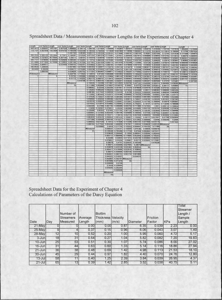
102
Spreadsheet Data / Measurements of Streamer Lengths for the Experiment of Chapter 4
L e n g th c o r r f a c to r L e n g th c o r r f a c to r L e n g th c o r r f a c to r L e n g th c o r r f a c to r L e n g th c o r r f a c to r L e n g th c o r r f a c to r L e n g th c o r r f a c to r L e n g th L e n g t h
0 .7 8 2 0 5 8 0 .9 9 1 8 6 6 0 .1 1 6 5 8 8 0 .866891 0 .8 1 9 6 3 5 0 .8 5 7 0 2 4d .1 8 1238 0 .038101 0 .2 /3 6 8 6 0 .048781 0 .3 6 2 7 0 5 0 .6 8 7 0 8 4
0 .O844O9 0 .6 2 7 6 1 3 0 .0 4 4 8 9 4 0 .3 2 8 6 0 3 0 .4 8 8 8 9 31 .02 4 0 1 6 0 .3 8 7 5 3 8 1.035893 0 .0 4 6 0 4 4 0 .085551 0 .6 2 6 2 2 5
3 0 .9 0 0 5 8 0 .0 7 0 2 8 6 0 .5 0 4 8 8 2 0 .4 0 4 7 0 8 0 .0 2 8 2 2 90 .1 1 0 8 5 3 0 .0 9 1 1 6 6 0 .077801 0 .0 8 5 1 7 2 0 .6 1 1 8 1 6 0 .1 5 2 3 8 8 0 .0 7 0 2 7 5 0 .4 9 7 0 9 3 0 .0 6 0 0 4 6 0 .4 3 9 5 2 9
0 .0 4 9 1 0 3 0 .4 0 2 3 5 7 0 .0 8 0 1 8 5 0 .0 7 8 9 5 6 0 .4 4 0 7 6 3 0 .0 6 0 9 2 90 .0 4 5 3 0 3 0 .9 5 0 1 5 8 0 .0 7 2 0 7 9 0 .0 6 2017 0 .0 6 7 5 3 7 0 .0 2 2 7 1 6 '0 .1 6 6 2 8 2
0 .026271 0 .2 1 5 0 5 3 0 .0 7 7 2 2 6 0 .0 8 1 1 3 9 0 .6 0 3 2 9 8 0 .0 4 0 9 9 6 0 .3 0 0 0 7 2 0 .0 3 8 5 8 2 0 .2 0 6 5 6 70 .8 4 5 9 0 7 0 .2 8 6 5 3 8 0 .8 8 2 8 7 5
# M e a s u r e # M e a s u r e c 0 .0 2 0 /9 8 b .0839 9 6 0 .6 0 3 3 6 4 0 .0 2 6 2 8 3 0 .0 2 2 5 7 6 0 .0 8 3 7 1 5 0 .0 1 9 3 4 90 .3 0 9 9 8 6 0 .0 9 8 9 2 6 0 .0 6 2 0 6 5 0 .3 0 6 3 7 5 0 .0 7 8 7 4 9 0 .557031 0 .0 3 0 4 6 4
0 .85 8 2 0 1 0 .0 8 5 4 0 3 0 .6 3 5 0 0 2 0 .3 3 8 6 9 3 0 .0 6 3 5 7 4 0 .0 4 1 7 0 7 0 .3 0 5 2 9 30 .8 6 0 1 4 5 0 .4 5 6 0 9 7 0 .063201 0 .4 6 2 5 9 8 0 .3 9 /2 9 5
0 .1 5 9 9 3 8 0 .5 1 4 8 0 5 0 .0 5 8 7 9 2 0 .0 6 0 6 8 9 S M e a s u r e d0 .8 0 5 9 6 4 0 .0 7 4 9 0 7 0 .5 3 8 0 7 5 0 .0 6 1 8 0 9
0 .0 8 6 6 6 2 0 .0 5 5 3 9 4 0 .3 9 7 9 0 7 0 .1 3 1 0 7 9 0 .9 7 4 6 2 8 0 .0 2 5 5 7 9 0 .0 7 0 7 2 5 0 .5 0 0 2 7 30 .0 9 2 4 5 8 0 .0 7 3 0 4 2 0 .5 8 6 3 6 2 0 .0 9 6 6 0 8 0 .6 8 3 3 5 50 .0 4 6 5 5 9 0 .0 6 0 9 2 9 0 .0 6 8 2 5 9 0 .4 8 2 8 2 90 .0 3 2 0 7 3 0 .2 3 0 3 8 6 0 .0 9 8 8 8 2 0 .0 8 3 0 6 9 0 .6 0 8 0 2
0 .1 0 1 8 3 8 0 .0 5 0 7 2 9 0 .5 3 8 5 5 2 0 .0 6 1 3 9 5 0 .0 7 6 8 5 0 .5 4 3 5 9 90 .0 5 8 5 0 2 0 .0 8 9 5 9 6 0 .0 9 9 0 7 2 0 .0 5 8 7 9 2 0 .4 3 0 3 2 9 0 .0 5 1 9 3 20 .0 7 6 3 1 9 0 .5 5 0 8 3 7 0 .0 4 4 6 8 5 0 .3 2 0 9 8 7 0 .1 0 7 7 9 50 .0 7 9 2 5 3 0 .0 3 4 6 6 2 0 .2 4 8 9 8 3 0 .776201 0 .1 0 1 0 70 .0 6 6 4 9 9 0 4 8 6 9 6 6 0 .0 9 5 7 5 4 0 .0 2 8 1 1 2 0 .1 9 8 8 5 4
0 .0 /6 8 5 1 0 .0 8 2 9 6 6 0 .6 1 6 8 8 5 0 .6 7 8 7 0 2 0 .0 3 8 2 6 60 .1 2 5 0 4 6 0 .5 3 1 7 0 5 0 .4 9 9 0 7 6 0 .1 2 6 1 8 5 0 .9 2 3 6 0 90.099951 0 .0 5 3 5 5 6 0 .3 8 4 7 0 6 0 .0 2 4 8 8 9 0 .1 8 5 0 5 6 0 .0 2 5 8 9 7 0 .1 8 3 1 8 50 .0 5 9 4 8 3 0 .3 8 /6 3 8 0 .0 9 0 0 3 2 0 .0 4 3 9 0 50 .0 6 2 8 2 9 0 .0 8 0 9 4 3 0 .63 7 6 0 1 0 .5 5 0 9 5 40 .0 7 7 3 6 8 0 .5 5 8 4 0 8 0 .0 6 6 1 6 4 0 .1 0 9 3 2 3 0 .81 2 8 6 2 0 .0 8 8 0 6 6 0 .0 3 6 2 4 80 .0 8 6 9 3 2 0 .0 7 7 8 9 8 0 .5 7 0 1 7 6
0 .0 6 4 0 4 6 0 .4 6 0 0 5 8 0 .1 6 7 9 8 7 0 .0 5 8 6 2 8 # M e a s u r e d0 .6 3 9 6 6 6 0 .9 0 8 9 9 7 0 .1 0 5 7 0 3
# M e a s u r e a 0 .0 8 8 2 6 0 .6 4 6 0 1 60 .1 0 9 3 4 9 0 .7 8 5 4 8 6 0 .0 9 2 2 6 30 .0 3 3 6 2 6 0 .2 8 4 6 4 6 0 .896561 0 .0 3 8 5 9 4 0 .2 8 2 4 9 20 .0 9 3 1 1 7 0 .6 6 8 8 8 6 0 .8 5 2 8 0 4 0 .0 2 0 2 6 8 0 .1 4 8 3 5 3
0 .0 7 1 9 1 4 0 .5 3 4 7 0 8 0 .0 4 9 4 6 4 0 .36 2 0 5 10 .076851
0 .0 2 4 9 3 5 0 .1 8 5 3 9 8 0 .4 7 6 2 2 60 .4 3 6 0 9 9 0 .0 2 7 8 0 5 I tM e a s u r e d
0 .0 5 9 8 7 6 0 .4 3 0 1 0 90 .0 8 0 4 7 7 0 .5 /8 0 8 8 0 .0 2 2 8 1 6
0 .4 3 6 0 9 9 0 .0 8 3 1 3 8 0 .6 1 8 1 6 40 .050221 0 .3 6 0 7 5 3 0 .0 9 1 7 1 9 0 .6 8 1 9 6 80 .044301
0 .302181 # M e a s u r e d0 .0 5 1 6 8 60 .0 3 8 0 8 9
0 .3 2 8 9 9 50 .0 3 3 2 9 5
0 .5 0 9 8 0 6I tM e a s u r e d
5 3 |
Spreadsheet Data for the Experiment of Chapter 4 Calculations of Parameters of the Darcy Equation
Date Day
Number of Streamers Measured
AverageLength
BiofilmThickness(mm)
Velocity(m/s) Diameter
FrictionFactor KPa
Total Streamer Length / Sample Length
21-May a 5 5 5 0 500 5 5 7 5735 0.039 2.23 5 5 525-May 5 3 0737 07T5 0755 5705 0.043 3.0/ TT3528-May TZ 5 5 2 5 2 0 T700 5755 OOtiO 4 /2 57T7
3-Jun 3T 5 5 3 0727 1.04 5752 0.082 7.20 T575310-Jun 25 53 55T 0730 1.07 5773 0.088 8.00 27752Iti-Jun 3T 33 5 5 3 5 5 0 1.33 57T3 O.llti 18 88 2775321-Jun 35 35 5 3 5 0755 TT32 3755 0.113 21.53 18.1030-Jun 35 25 5 3 3 0757 T752 3730 0.0/0 24./ti T2755IikJuI 55 ^TT 5 3 0 1.25 2735 3753 0.039 28.95 373721-Jul 55 T 3 0735 1.42 2755] 3752 0.038 40./5 57TT
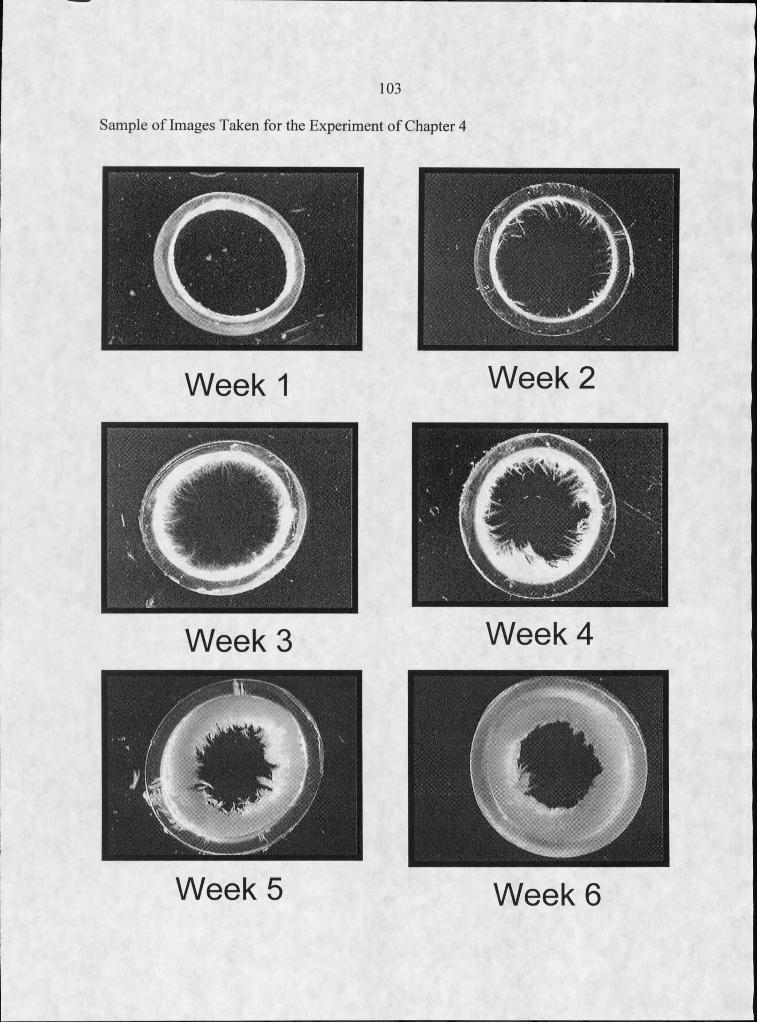
103
Sample of Images Taken for the Experiment of Chapter 4
Week 1 Week 2
Week 3
Week 5 Week 6

104
APPENDIX B
EXPERIMENTAL DATA RELEVANT TO CHAPTER 5
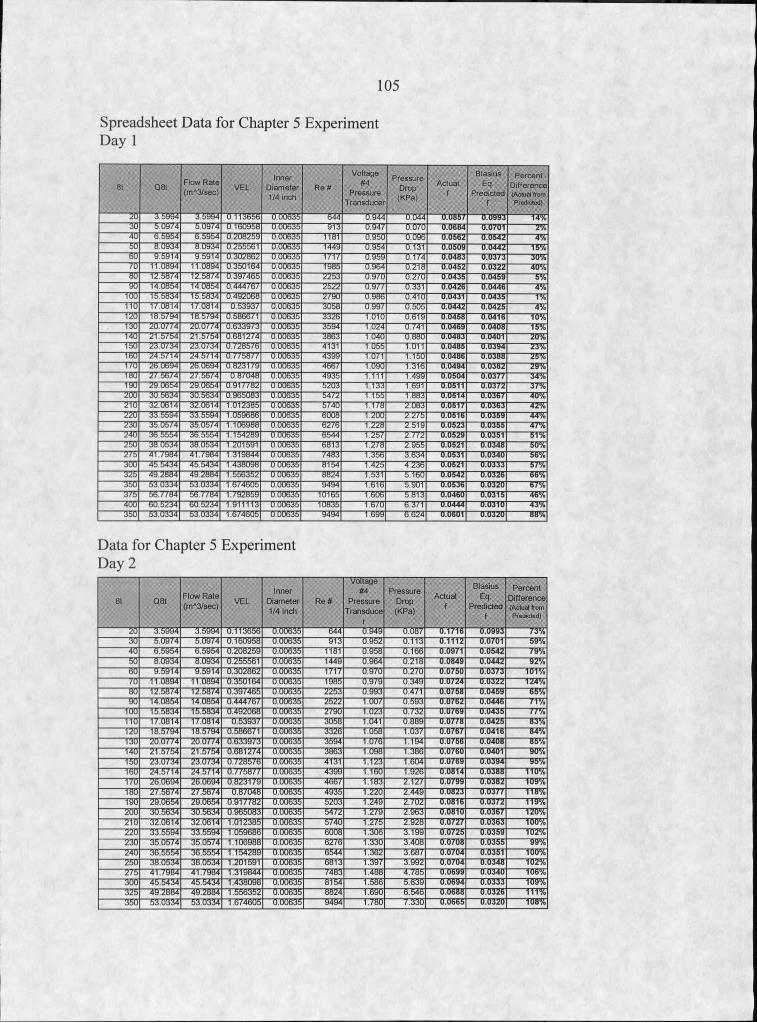
105
Spreadsheet Data for Chapter 5 ExperimentDay I
8t Q8tFlow R ate (m A3/sec) VEL
Im er D iam eter 1/4 inch
R e #
Voltage#4
P ressu reT ransducer
P ressu reDrop
(KPa)
Actualf
BlasiusEq-
Predicted. f
P ercen tDifference(Actual from Predicted)
" 20 ^ 3 ^ 5 9 9 4 3.5994 O t 15666 0.00635 .. 644 0.944 6.044 0.0857 6.6993 14 Vo30 5 .0 9 /4 5 .0 9 /4 0 .160958 0.00635 5TB 0.947 0 .0 /0 0.0684 0.0701 2%30 6.5954 6.5954 0.208259 0.00635 1181 0.950 0.096 0.0562 0.0542 4%50 8.0934 8.0934 0.255561 0.00635 1449 0.954 0.131 0.0509 0.0442 15%60 9.5914 9.5914 0.302862 0.00635 1 /1 / 0.959 0 .1 /4 0.0483 0.0373 3D%fO 11.0894 11.0894 0.350164 0.00635 1985 0,964 0.218 0.0452 0.0322 40%BO 12 .5 8 /4 1 2 .5 8 /4 0 .3 9 /4 6 5 0.00635 2253 0 .9 /0 0 .2 /0 0.0435 0.0459 5%90 14.0854 14.0854 0.444767 0.00635 2522 0 .9 /7 0.331 0.0426 0.0446 4%
TOO 15.5834 15.5834 0.492068 0.00635 2 /9 0 0.986 0.410 0.0431 0.0435 T%17.0814 0.53937 0.00635 3058 0.997 0.505 0.0442 0.0425 4%
T20 18.5794 1 8 .5 /94 0 .5866 /1 0.00635 3326 1.010 0.619 0.0458 0.0416 10%T30 2 0 .0 / /4 2 0 .0 7 /4 0 .6 3 3 9 /3 0.00635 3594 1.024 0. /41 0.0469 0 .0 4 0 8 T5%T30 2 1 .5 /5 4 2 1 .5 /5 4 0 .6 8 1 2 /4 0.00635 3863 1.040 0.880 0.0483 0.0401 20%150 0.728576 0.00635 4131 1.055 1.011 0.0485 0.0394 23%TOO 24.5714 24.5714 0 . / / 5 8 /7 0.00635 4399 1.0/1 1.150 0.0486 0.0388 25%T70 26.0694 26.0694 0.823179 0.00635 4 6 6 / 1.090 1.316 0.0494 0.0382 29%TBO 2 / 5 6 / 4 27.5674 0.87048 0.00635 4935 1.111 1.499 0.0504 0.0377 34%T90 29.0654 29.0654 0 .9 1 7 /8 2 0.00635 5203 1.133 1.691 0.0511 0.0372 37%200 30.5634 30.5634 0.965083 0.00635 5 4 /2 1.155 1.883 0.0514 0.0367 40%2TU 32.0614 32.0614 1.012385 0.00635 5 /4 0 1 .1 /8 2.083 0.0517 0.0363 42%220 33.5594 33.5594 1.059686 0.00635 6008 1.200 2 .2 /5 0.0516 0.0359 44%230 35.0574 35.0574 1.106988 0.00635 6276 1.228 2.519 0.0523 0.0355 47%230 36.5554 36.5554 1. 154289 0.00635 6544 1 .2 5 / 2. / / 2 0.0529 0.0351 51%250 38.0534 38.0534 1.201591 0.00635 6813 1 .2 /8 2.955 0.0521 0.0348 50%275 4 1 ./9 8 4 41.7984 1.319844 0.00635 7483 1.356 3.634 0.0531 0.0340 55%300 45.5434 45.5434 1.438098 0.00635 8154 1.425 4.236 0.0521 0.0333 57%325 49.2884 49.2884 1.556352 0.00635 8824 1.531 5.160 0.0542 0.0326 55%350 53.0334 53.0334 1 .6 /4 6 0 5 0.00635 9494 1.616 5.901 0.0536 0.0320 67%375 5 6 . / /8 4 5 6 .7 /5 4 I . /92859 0.00635 10165 1.606 5.813 0.0460 0.0315 46%300 60.5234 60.5234 1.911113 0.00635 10835 1 .6 /0 6 .3 /1 0.0444 0.0310 43%350 53.0334 53.0334 1 .6 /4 6 0 5 0.00635 9494 1.699 6.624 0.0601 0.0320 88%
Data for Chapter 5 Experiment Day 2
81 081 Flow R ate (m A3/sec) VEL
Inner D iam eter 1/4 inch
R e #
V oltage#4
P ressu reT ran sd u ce
: r ■
P ressu reDrop
(KPa)
Actualf
BlasiusEq-
Predictedf
P ercen tD ifference(Actual from Predicted)
20 3.5994 3.5994 6.113856 8.00635 644 0.949 0.687 0 .1 )1 6 0.0993 ... 73%30 5 .0 9 /4 5 .0 9 /4 0.160958 0.00635 3T3 0.952 0.113 0.1112 0.0701 55%40 6.5954 6.5954 0.208259 0.00635 1181 0.958 0.166 0.0971 0.0542 75%50 8.0934 8.0934 0.255561 0.00635 1449 0.964 0.218 0.0849 0.0442 52%BO 9.5914 9.5914 0.302862 0.00635 1717 0.970 0.270 075750 0.0373 101%70 11.0894 11.0894 0.350164 0.00635 1985 0.979 0.349 0.0724 0.0322 124%80 1 2 .5 8 /4 12.5874 0.397465 0.00635 2253 0.993 0.471 0.0758 0.0459 55%SO 14.0854 14.0854 0.444767 0.00635 2522 1.007 0.593 0.0762 0.0446 7T%
TOO 15.5834 15.5834 0.492068 0.00635 2790 1.023 0.732 0 .0 /6 9 0.0435 77%TTO 17.0814 17.0814 0.53937 0.00635 3058 1.041 0 .889 0.0778 0.0425 83%T20 18.5794 18.5794 0.586671 0.00635 3326 1.058 1.037 0.0767 0.0416 84%T30 20.0774 20.0774 0.633973 0.00635 3594 1.076 1.194 0.0756 0.0408 85%T40 21.5754 21.5754 0.681274 0.00635 3863 1.098 1.386 0.0760 0.0401 90%T50 23.0734 23.0734 0.728576 0.00635 4131 1.123 1.604 0.0769 0.0394 55%TBa 24.5714 24.5714 0.775877 0.00635 4399 1.160 1.926 0.0814 0.0388 110%TTO1 26.0694 26.0694 0.8231 /9 0 .00635 4667 1.183 2TT77 0.0799 0.0382 109%TBO1 27.5674 2 / .5 6 /4 0 .87048 0.00635 4935 1.220 2.449 0.0823 0.0377 118%TSO1 29.0654 29.0654 0.917782 0.00635 5203 1.249 2.702 0.0816 0.0372 119%203 30.8634 80.5634 0.965083 0.00635 5472 1.279 2.963 0.0810 0.0367 120%2TTT 32.0614 32.0614 1(112385 U.UU635 57401 1.275 2.928 0.0727 0.0363 100%223 33.5594 33.5594 1.059686 0.00635 6008 1.306 3 .199 0.0725 0.0359 102%23G 35.0574 35.0574 1.106988 0.00635 6 2 /6 1.330 3 .408 0.0708 0.0355 55%243 36.5554 36.5554 1.154289 0.00635 6544 1.362 3.687 0.0704 0.0351 100%253 38.0534 38.0534 1.201591 0.00635 6813 1357 3 5 5 7 0.0704 0.0348 102%275' 41.7984 41.7984 1.319844 0.00635 7483 1.488 4 .785 0.0699 0.0340 106%30ff 45.5434 45.5434 1.438098 0.00635 5T54 1330 57035 0.0694 0.0333 109%325 49 .2884 49.2884 1.556352 0.00635 8824 1.690 6 .546 0.0688 0.0326 111%353 53.0334 53.0334 1.674605 U.UUO&L 9494 1.780 7.330 0.0665 0.0320 108%
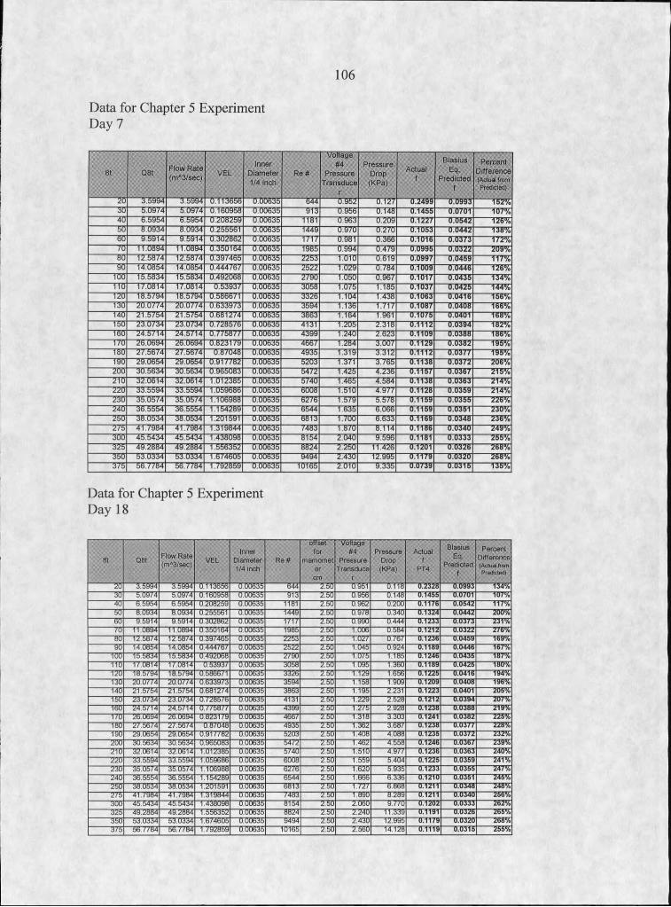
Data for Chapter 5 ExperimentDay 7
106
Bt QBtFlow R a te (m A3 /se c )
VELInner
D ia m e te r 1 /4 inch
R e #
V oltage#4
P re ss u reT ra n sd u c e
:: I r
P re s s u reD rop
(K P a)
A ctualf
B las iu sEq.
P re d ic te df
P e rc e n t D iffe ren ce (Actual from Predicted)
.Io1 3 .5 9 9 4 3 .5 9 9 4 0 .1 1 3 6 5 6 ~trnoB35 644 cT9S2 0 .1 2 7 0.2499 0.0993 152%3U" 5 .0 9 7 4 5 .0 9 7 4 0 .1 6 0 9 5 8 0 .0 0 6 3 b 9TT 0 .9 5 6 0 .1 4 8 0 .1 4 5 5 0.0701 T07%30 6 5 9 5 4 6 .5 9 5 4 0 .2 0 8 2 5 9 0 .0 0 6 3 5 TTET 0 .9 6 3 0 .2 0 9 0 .1 2 2 7 0 .0 5 4 2 126%50 8 .0 9 3 4 8 .0 9 3 4 0 .255561 0 .0 0 6 3 5 1449 0 .9 7 0 0 .2 7 0 0 .1 0 5 3 0 .0 4 4 2 138%50 9 .5 9 1 4 9 .5 9 1 4 0 .3 0 2 8 6 2 0 .0 0 6 3 5 1717 0.981 0 .3 6 6 0 .1 0 1 6 0 .0 3 7 3 172%70 1 1 .0 8 9 4 11 .0 8 9 4 0 .3 5 0 1 6 4 0 .0 0 6 3 5 1985 0 .9 9 4 0 .4 7 9 0 .0 9 9 5 0 .0 3 2 2 209%50 1 2 .5 8 7 4 12 .5 8 7 4 0 .3 9 7 4 6 5 0 .0 0 6 3 5 2 253 1 .010 0 .6 1 9 0 .0 9 9 7 0 .0 4 5 9 117%50 1 4 .0 8 5 4 14 .0 8 5 4 0 .4 4 4 7 6 7 0 .0 0 6 3 5 2 522 1 .029 0 .7 8 4 0 .1 0 0 9 0 .0 4 4 6 126%
TOO 1 5 .5 8 3 4 15 .5 8 3 4 0 .4 9 2 0 6 8 0 .0 0 6 3 5 2 7 9 0 1.050 0 .9 6 7 0 .1 0 1 7 0 .0 4 3 5 1 34%TTO 1 7 .0 8 1 4 17 .0 8 1 4 0 .5 3 9 3 7 0 .0 0 6 3 5 305 8 1.075 1 .185 0 .1 0 3 7 0 .0 4 2 5 144%TZO 1 8 .5 7 9 4 18 .5 7 9 4 0 .586671 0 .0 0 6 3 5 3 3 2 6 1 .104 1.438 0 .1 0 6 3 0 .0 4 1 6 156%TOO 2 0 .0 7 7 4 2 0 .0 7 7 4 0 .6 3 3 9 7 3 0 .0 0 6 3 5 359 4 T7T35 1 .717 0 .1 0 8 7 0 .0 4 0 8 166%T30 2 1 .5 7 5 4 2 1 .5 7 5 4 0 .6 8 1 2 7 4 0 .0 0 6 3 5 386 3 1 .164 1.961 0 .1 0 7 5 0 .0401 168%T50 2 3 .0 7 3 4 2 3 .0 7 3 4 0 .7 2 8 5 7 6 0 .0 0 6 3 5 4131 1 .205 2 .3 1 8 0 .1 1 1 2 0 .0 3 9 4 182%T50 2 4 .5 7 1 4 2 4 .5 7 1 4 0 .7 7 5 8 7 7 0 .0 0 6 3 5 4 3 9 9 1 .240 2 .6 2 3 0 .1 1 0 9 0 .0 3 8 8 186%T70 2 6 .0 6 9 4 2 6 .0 6 9 4 0 .8 2 3 1 7 9 0 .0 0 6 3 5 466 7 1 .284 3 .0 0 7 0 .1 1 2 9 0 .0 3 8 2 195%TOO 2 7 .5 6 7 4 2 7 .5 6 7 4 0 .8 7 0 4 8 0 .0 0 6 3 5 4 9 3 5 1 .319 3 .3 1 2 0 .1 1 1 2 0 .0 3 7 7 19 5 %TOO 2 9 .0 6 5 4 2 9 .0 6 5 4 0 .9 1 7 7 8 2 0 .0 0 6 3 5 520 3 1.371 3 .7 6 5 0 .1 1 3 8 0 .0 3 7 2 206%ZOO 3 0 .5 6 3 4 3 0 .5 6 3 4 0 .9 6 5 0 8 3 0 .0 0 6 3 5 5472 1 .425 4 .2 3 6 0 .1 1 5 7 0 .0 3 6 7 215%ZTO 3 2 .0 6 1 4 3 2 .0 6 1 4 1 .0 1 2 3 8 5 0 .0 0 6 3 5 574 0 1 .465 4 .5 8 4 0 .1 1 3 8 0 .0 3 6 3 214%ZZO 3 3 .5 5 9 4 3 3 .5 5 9 4 1 .0 5 9 6 8 6 0 .0 0 6 3 5 600 8 1 .510 4 .9 7 7 0 .1 1 2 8 0 .0 3 5 9 214%Z30 3 5 .0 5 7 4 3 5 .0 5 7 4 1 .1 0 6 9 8 8 0 .0 0 6 3 5 6 2 7 6 1 .579 5 .5 7 8 0 .1 1 5 9 0 .0 3 5 5 226%230 3 6 .5 5 5 4 3 6 .5 5 5 4 1 .15 4 2 8 9 0 .0 0 6 3 5 6 5 4 4 1 .635 6 .0 6 6 0 .1 1 5 9 0 .0351 230%250 3 8 .0 5 3 4 3 8 .0 5 3 4 1 .201591 0 .0 0 6 3 5 6 8 1 3 1 .700 6 .6 3 3 0 .1 1 6 9 0 .0 3 4 8 236%275 4 1 .7 9 8 4 4 1 V 9 8 4 1 .3 1 9 8 4 4 0 .0 0 6 3 5 7483 1.870 8 .1 1 4 0 .1 1 8 6 0 .0 3 4 0 249%300 4 5 .5 4 3 4 4 5 .5 4 3 4 1.4 3 8 0 9 8 0 .0 0 6 3 5 815 4 2 .0 4 0 9 .5 9 6 0.1181 0 .0 3 3 3 255%325 4 9 .2 8 8 4 4 9 .2 8 8 4 1 .556 3 5 2 0 .0 0 6 3 5 882 4 2 .2 5 0 1 1 .426 0.1201 0 .0 3 2 6 268%350 5 3 .0 3 3 4 5 3 .0 3 3 4 1 .674 6 0 5 0 .0 0 6 3 5 949 4 2 .4 3 0 12 .995 0 .1 1 7 9 0 .0 3 2 0 268%375 5 6 .7 7 8 4 5 6 .7 7 8 4 1 .7 9 2 8 5 9 0 .0 0 6 3 5 10165 2 .0 1 0 9 .3 3 5 0 .0 7 3 9 0 .0 3 1 5 135%
Data for Chapter 5 Experiment Day 18
8 t Q S t F l o w R a t e ( m A 3 / s e c ) V E L
I n n e r D i a m e t e r
1 / 4 i n c hR e #
o f f s e tf o r
m a m o m e te r
c m
V o l t a g e# 4
P r e s s u r eT r a n s d u c e
r
P r e s s u r eD r o p
( K P a )
A c t u a lf
P T 4
B l a s i u sE q -
P r e d i c t e df
P e r c e n tD i f f e r e n c e(Actual from Predcted)
20 3.5994 3.5994 0.113656 6.60335 OT 5b 0.951 0T l8 0 .2 3 2 8 0 .0 9 9 3 1 3 4 %3 0 5.0974 5 .0 9 /4 0.160958 0.00635 B T B 2.50 E T S i S 0.148 0 .1 4 5 5 0 .0 /0 1 1 0 7 %4 0 6.5954 6.5954 0 208259 0.00635 1181 2.50 0.962 0.200 0 .1 1 7 6 0 .0 5 4 2 117%5 0 8.0934 8.0934 0.255561 0.00635 1449 2.50 0.978 0.340 0 .1 3 2 4 0 .0 4 4 2 200%B O 9.5914 9.5914 0.302862 0.00635 1717 2.50 0.990 0.444 0 .1 2 3 3 0 .0 3 7 3 231%
7 0 11.0894 11.0894 0.350164 0.00635 1985 2.50 1.006 0.584 0 .1 2 1 2 0 .0 3 2 2 276%B O 12.5874 1 2 .58 /4 0 .3 9 /4 6 5 0.00635 2253 2.50 1.027 0.767 0 .1 2 3 6 0 .0 4 5 9 169%5 0 14.0854 14.0854 0 .4 4 4 /6 / 0.00635 2522 2.50 1.045 0.924 0 .1 1 8 9 0 .0 4 4 6 167%
T O O 15.5834 15.5834 0.492068 0.00635 2790 2.50 1.075 1.185 0 .1 2 4 6 0 .0 4 3 5 187%T T O j 1/.UB14 17.0814 0.53937 0.00635 3 0 5 8 2.50 1.095 1.360 0 .1 1 8 9 0 .0 4 2 5 180%T Z O - T E T B T S R 18.5794 0.586671 0.00635 3326 2.50 1.129 1.656 0 .1 2 2 5 0 .0 4 1 6 194%T 3 0 - 20.0774 2 0 .0 /7 4 0.633973 0.00635 3594 2.50 1.158 1.909 0 .1 2 0 9 0 .0 4 0 8 196%T 4 0 " 2 1 .5 /5 4 21.5754 0 .6 8 1 2 /4 0.00635 3863 2.50 1.195 2.231 0 .1 2 2 3 0 .0 4 0 1 205%T 5 0 " 2B.U/3 4 I 23.0734 0.728576 0.00635 4131 2.50 1.229 2.528 0 .1 2 1 2 0 .0 3 9 4 207%T B O - 2 4 .5 /1 4 2 4 .5 /1 4 0.775877 0.00635 4399 2.50 1.275 2.928 0 .1 2 3 8 0 .0 3 8 8 219%T T O - 26.0694 26.0694 0.8231 79 0.00635 4667 2.50 1.318 3.303 0 .1241 0 .0 3 8 2 225%T B B 27.5674 27.5674 0 .8 /0 4 8 0.00635 4935 2.50 1.362 3.687 0 .1 2 3 8 0 .0 3 7 7 228%T W 29.0654 29.0654 0.917782 0.00635 5203 2.50 1.408 4.088 0 .1 2 3 5 0 .0 3 7 2 2 3 2 %
Z O B 30.5634 30.5634 0.965083 0.00635 5472 2.50 1.462 4.558 0 .1 2 4 6 0 .0 3 6 7 2 3 5 %2 W 32.0614 32.0614 1.012385 0.00635 5740 2.50 1.510 3 T 3 7 7 0 .1 2 3 6 0 .0 3 6 3 240%Z Z B 3 3 . 5 5 9 4 33.5594 1.059686 0.00635 6008 2.50 1.559 5.404 0 .1 2 2 5 0 . 0 3 5 9 241%2 3 1 T 35.0574 35.0574 1.106988 0.00635 6276 2.50 1.620 5.935 0 .1 2 3 3 0 .0 3 5 5 247%2 4 B 36.5554 36.5554 1.154289 0.00635 6544 2.50 T T S G S 6.336 0 .1 2 1 0 0 .0 3 5 1 245%Z 5 B 38.0534 38.0534 1.201591 0. UlXxii 6813 2.50 1.727 6.868 0.1211 0 .0 3 4 8 248%275 41.'/984 41.7984 1.319844 0.00635 7483 2.50 1.890 8.289 0 .1211 0 .0 3 4 0 256%B O B 45.5434 45.5434 1 . 4 3 a U 9 H O.UlXxJb B T B T 2.50 2.060 9.7 70 0 .1 2 0 2 0 .0 3 3 3 262%B Z B 49.4884 49.2884 1.556352 0.00635 8824 2.50 2.240 11.339 0.1191 0 .0 3 2 6 265%3 5 B 53.0334 53.0334 1.674605 0.00635 9494 2.50 2.430 12.995 0 .1 1 7 9 0 .0 3 2 0 268%3 7 B 56.7784 56.7784 1.792859 0.00635 10165 2.50 2.560 14.128 0 .1 1 1 9 0 .0 3 1 5 255%
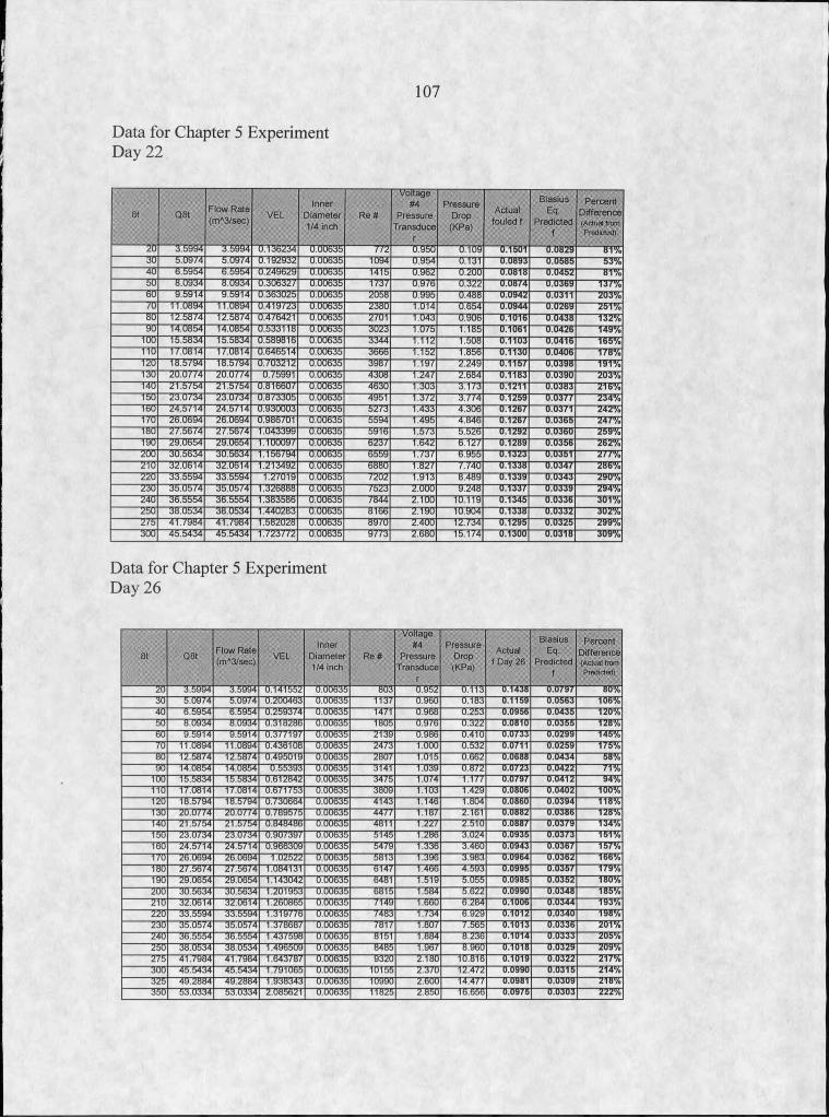
Data for Chapter 5 ExperimentDay 22
107
8 t Q StFlow R a te (m A3 /se c )
VELInner
D iam eter 1/4 inch
R e #
V oltage#4
P re ssu reT ra n sd u c e
r
P re ss u reDrop
(K Pa)
Actual fou led f
B lasiu sEq.
P red ic tedf
P e rc e n tD iffe rence(Actual from Predicted)
" Io 3 .5 9 9 4 3 .5 9 9 4 0.138234 ~ThtoB35 772 olSo U.109 0.1501 0.0829 -gnpj£
30 8 .0 9 /4 5 .0 9 /4 0 .1 9 2 9 3 2 0 .0 0 6 3 5 1094 0 .9 5 4 0.131 0 .0893 0 .0 5 8 5 53%30 6 .5 9 8 4 6 .5 9 5 4 0 .2 4 9 6 2 9 0 .0 0 6 3 5 1415 0 .962 0 .2 0 0 0 .0818 0.0452 81%50 8 .0 9 3 4 8 .0 9 3 4 0 .3 0 6 3 2 / 0 .0 0 6 3 5 1 /3 7 0 .9 /6 0 .3 2 2 0 .0 8 /4 0 .0 3 6 9 13/Vo50 9 .5 9 1 4 9 .5 9 1 4 0 .3 6 3 0 2 5 0 .0 0 6 3 5 2058 0 .9 9 5 0 .4 8 8 0 .0942 0.0311 2 0 3 Vo70 11 .0 8 9 4 11 .0894 0 .4 1 9 /2 3 0 .0 0 6 3 5 238 0 1.014 0 .6 5 4 0 .0 9 4 4 0 .0 2 6 9 251%50 12.58 /4 12 .5874 0 .4 /6 4 2 1 0 .0 0 6 3 5 2701 1.043 0 .906 0 .1016 0 .0 4 3 8 132%go 14 .0854 14 .0854 0 .5 3 3 1 1 8 0 .0 0 6 3 5 3 023 1 .0 /5 1.185 0.1061 0 .0 4 2 6 149%
TOO 15 .5 8 3 4 15 .5 8 3 4 0 .5 8 9 8 1 6 0 .0 0 6 3 5 3344 1 .112 1.508 0 .1103 0.0416 165%TTO 17 .0 8 1 4 17 .0 8 1 4 0 .6 4 6 5 1 4 0 .0 0 6 3 5 3 666 1.152 1.856 0 .1130 0 .0 4 0 6 178%TZO 1 8 .5 /9 4 1 8 .5 /9 4 0 ./0 3 2 1 2 O.Oueas 3987 1.197 2 .2 4 9 0 .1157 0 .0 3 9 8 191 VoTOO 2 0 .0 / / 4 2 0 .0 / / 4 0 ./5 9 9 1 0 .0 0 6 3 5 4 308 1.247 2 .684 0 .1183 0 .0 3 9 0 203%T30 2 1 .5 /5 4 2 1 .5 /5 4 0 .8 1 6 6 0 / 0 .0 0 6 3 5 4 630 1.303 3 .1 /3 0.1211 0.0383 216%T50 2 3 .0 /3 4 Z 3 .0 /3 4 0 .8 /3 3 0 5 0 .0 0 6 3 5 4951 1.372 3 . / / 4 0 .1259 0.0377 234%TOO 2 4 .5 /1 4 2 4 .5 /1 4 0 .9 3 0 0 0 3 0 .0 0 6 3 5 5 2 /3 1.433 4 .3 0 6 0 .1267 0.0371 242%TTO 2 6 .0 6 9 4 26 .0 6 9 4 0 .9 8 6 /0 1 0 .00 6 3 5 5594 1.495 4 .8 4 6 0 .1267 0 .0 3 6 5 247%TBO 2 / 5 6 / 4 2 / 5 6 / 4 1 .043399 0 .00 6 3 5 5 916 1 .5 /3 5 .526 0 .1292 0.0360 259%TOO 2 9 .0 6 5 4 2 9 .0 6 5 4 1 .1 0 0 0 9 / 0 .00 6 3 5 6 2 3 / 1.642 6 .1 2 / 0 .1289 0.0356 262%ZOO 3 0 .5 6 3 4 3 0 .5 6 3 4 1 .1 5 6 /9 4 0 .00 6 3 5 6 559 I . / 3 / 6 .9 5 5 0 .1323 0.0351 2 //V oZTO 3 2 .0 6 1 4 3 2 .0 6 1 4 1.213492 0 .00 6 3 5 6 880 1 .8 2 / / . / 4 0 0 .1338 0 .0 3 4 / 286%ZZO 3 3 .5 5 9 4 3 3 .5 5 9 4 1 .2 /0 1 9 0 .00 6 3 5 /2 0 2 1.913 8 .489 0 .1339 0 .0 3 4 3 290%ZOO 3 5 .0 5 /4 3 5 .0 5 /4 1 .326888 0 .00 6 3 5 /5 2 3 2 .0 0 0 9 .2 4 8 0 .1 3 3 / 0 .0 3 3 9 294%Z30 3 6 .5 5 5 4 3 6 .5 5 5 4 1.38 3 5 8 6 0 .00 6 3 5 /8 4 4 2 .100 10.119 0.1345 0 .0 3 3 6 3 0 1 Vo250 3 8 .0 5 3 4 3 8 .0 5 3 4 1 .440283 0 .0 0 6 3 5 8166 2 .1 9 0 10.904 0.1338 0 .0 3 3 2 302%Z75 4 1 / 9 8 4 4 1 / 9 8 4 1.582028 0 .0 0 6 3 5 8 9 /0 2 .4 0 0 12 . /3 4 0.1295 0 .0 3 2 5 299%300 4 5 .5 4 3 4 4 5 .5 4 3 4 I . / 2 3 / / 2 O.QOBSb 9 / / 3 2 .6 8 0 15.1 /4 0 .1300 0 .0318 309%
Data for Chapter 5 Experiment Day 26
Bt QStFlow R a te (m A3/sec) V E L
Inner D iam eter 1/4 inch
R e #
V oltage#4
P re ssu reT ran sd u ce
r
P re ssu reD rop(K Pa)
Actual f Day 26
BlasiusEq-
P red ic tedf
P e rce n t D ifference ( A c tu a l f r o m
P r e d i c t e d )
' 20 3 .5994 3 .5994 0.1 T l 652 0 .00636 BOB 6.952 0 .113 0.1438 0 .0 / 9 7 " 5 0 %30 5 .0 9 /4 5 .0 9 /4 0 .200463 0 .00635 1137 0 .960 0 .183 0.1159 0 .0563 106%TO 6.5954 6 .5954 0.259374 0.00635 1471 0 .968 0 .253 0.0956 0 .0435 120%50 S.U9S4 8 .0934 0.318286 0.00635 T805 0 .9 /6 0 .322 0.0810 0 .0355 1 28%BO 9.5 9 1 4 9 .5914 0 .377197 0.00635 2139 0 .986 0 .410 0 .0 /3 3 0 .0299 145%70 11.0894 11.0894 0.436108 0.00635 2473 1.000 0 .532 0.0711 0 .0259 175%80 12.5874 12.5874 0.495019 0.00635 2807 1.015 0 .662 0.0688 0 .0434 5 5 %go 14.US54 14.0854 0.55393 0.UUS3S 3141 1.039 0 .872 0.0723 0 .0422 7T%
TOO 15.5834 15.5834 0 .612842 0.00635 3475 1 .0 /4 1.177 0.0797 0 .0412 94%TTO 17.0814 17.0814 0 .6 /1 7 5 3 0.00635 3809 1.103 1.429 0.0806 0 .0402 100%TZO 18.5794 1 8 .5 /9 4 0 ./3 0 6 6 4 0.00635 4143 1.146 1.804 0.0860 0 .0 3 9 4 118%TOO 20.0774 2 0 .0 7 /4 0. /8 9 5 /5 0 .00635 4 4 7 / 1 .1 8 / 2.161 0.0882 0 .0386 128%TTO 21.5754 21 .5754 0.848486 0.00635 4811 TT227 ZTBTff 0.0887 O T B B T B T33%T50 23 .0 7 3 4 23 .0734 0 .9 0 /3 9 / 0 .00635 5145 1.286 3.024 0.0935 0 .0373 151%TBO 24.8714 2 4 .5 /1 4 0 .966309 0.00635 5479 1.336 3.460 0.0943 0 .0367 157%TTO 26 .0694 26 .0694 1 .02522 0.00635 5813 1.396 BTBBB 0.0964 0 .0362 166%TBO 2 7 .5 6 /4 2 7 .5 6 /4 1.084131 0.00635 6147 1.466 TBBB 0.0995 0.0357 179%TOO 29.0654 29 .0664 1.143042 0.00635 6481 1.519 5.055 0.0985 0 .0352 180%ZOO 30.5 6 3 4 30.5634 1 .201953 0.00635 6815 1.SB4 5.622 0.0990 0 .0348 185%ZTO 32.0 6 1 4 32.0614 1 .260865 0.00635 7T39 TTBBff 6 .284 0.1006 0.0344 193%ZZOj 33 .5 5 9 4 33.5594 1 .3 1 9 /7 6 0.00635 /4 8 3 1.734 6.929 0.1012 0 .0340 198%Z30" 35 .0574 35.0574 1.378687 0.00635 / 8 1 / 1 .8 0 / 7.565 0.1013 0.0336 201%ZTO- 36 .5554 36 .5554 1 .437598 0.00635 8151 1.884 8.236 0.1014 0.0333 205%Z 5 a 38 .0 5 3 4 38.0534 1.4965U9 0.00635 8485 1.967 8.960 0.1018 0.0329 209%275 41 .7 9 8 4 41 .7984 1 .6 4 3 /8 7 0.00635 9320 2.180 10.816 0.1019 0.0322 217%3 0 0 45 .5 4 3 4 45 .5434 1.791065 0.00635 10155 2 .3 /0 12.472 0.0990 0.0315 214%325 49 .2 8 8 4 49 .2 8 8 4 1.938343 0.00635 10990 2.600 14.477 0.0981 0.0309 218%350“ 53 .0334 53 .0334 2.085621 0 .00635 11825 2.850 16.656 0.0975 0.0303 222%
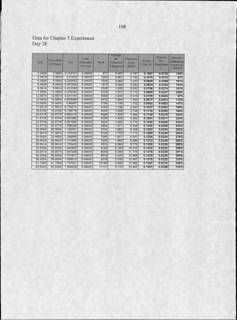
108
Data for Chapter 5 ExperimentDay 28
081 Flow Rate (m'‘S/sec) VEL
Inner Diameter 1/4 inch
R e#
Voltage# 4
PressureTransduce
r
PressureDrop(KPa)
Actual f Day 32
BlasiusEq-
Predictedf
Percent Difference
( A c t u a l f r o m P r e d i c t e d )
3 . 5 6 9 4 5 . 1 5 4 7 4 7 0 . 0 0 6 3 5 # 7 0 . 9 5 7 0 . 1 5 7 0.1667 0.0729 i 28%5 . 0 9 7 4 5 . 0 9 7 4 0 . 2 1 9 1 5 0 . 0 0 6 3 5 I W 0 . 9 6 1 0 . 1 9 2 0.1016 0.0515 97%6 . 5 9 5 4 6 . 5 9 5 4 0 . 2 8 3 5 5 3 0 . 0 0 6 3 5 TBM 0 . 9 6 8 0 . 2 5 3 0.O8OO 0.0398 101%8 . 0 9 3 4 8 . 0 9 3 4 0 . 3 4 7 9 5 6 0 . 0 0 6 3 5 T W 0 . 9 8 4 0 . 3 9 2 0.0824 0.0324 154%9 . 5 9 1 4 9 . 5 9 1 4 0 . 4 1 2 3 5 9 0 . 0 0 6 3 5 2 3 3 8 1 . 0 0 0 0 . 5 3 2 0.0796 0.0274 191%
1 1 . 0 8 9 4 1 1 . 0 8 9 4 0 . 4 7 6 7 6 2 0 . 0 0 6 3 5 2 7 0 3 1 . 0 2 1 0 . 7 1 5 0.0800 0.0237 238%1 2 . 5 8 7 4 1 2 . 5 8 7 4 0 . 5 4 1 1 6 5 0 . 0 0 6 3 5 3 0 6 8 1 . 0 4 4 0 . 9 1 5 0.0795 0.0425 87%1 4 . 0 8 5 4 1 4 . 0 8 5 4 0 . 6 0 5 5 6 8 0 . 0 0 6 3 5 3 4 3 3 1 . 0 8 4 1 . 2 6 4 0.0877 0.0413 112%1 5 . 5 8 3 4 1 5 . 5 8 3 4 0 . 6 6 9 9 7 0 . 0 0 6 3 5 3 7 9 8 1 . 1 4 0 1 . 7 5 2 0.0993 0.0403 147%1 7 . 0 8 1 4 1 7 . 0 8 1 4 0 . 7 3 4 3 7 3 0 . 0 0 6 3 5 4 1 6 4 1 . 1 9 6 2 . 2 4 0 0.1057 0.0393 169%1 8 . 5 7 9 4 1 8 . 5 7 9 4 0 . 7 9 8 7 7 6 0 . 0 0 6 3 5 4 5 2 9 1 . 2 6 0 2 . 7 9 8 0.1116 0.0385 190%
2 0 . 0 7 7 4 2 0 . 0 7 7 4 0 . 8 6 3 1 7 9 0 . 0 0 6 3 5 1 . 3 2 5 3 . 3 6 4 0.1149 0.0378 204%2 1 . 5 7 5 4 2 1 . 5 7 5 4 0 . 9 2 7 5 8 2 0 . 0 0 6 3 5 5 2 5 9 1 . 4 0 5 4 . 0 6 2 0.1201 0.0371 224%2 3 . 0 7 3 4 2 3 . 0 7 3 4 0 . 9 9 1 9 8 5 0 . 0 0 6 3 5 5 6 2 4 1 . 4 8 0 4 . 7 1 5 0.1220 0.0365 234%2 4 . 5 7 1 4 2 4 . 5 7 1 4 1 . 0 5 6 3 8 8 0 . 0 0 6 3 5 5 9 8 9 1 . 5 7 1 5 . 5 0 8 0.1256 0.0359 250%2 6 . 0 6 9 4 2 6 . 0 6 9 4 1 . 1 2 0 7 9 1 0 . 0 0 6 3 5 6 3 5 4 1 . 6 6 5 6 . 3 2 8 0.1282 0.0354 262%2 7 . 5 6 7 4 2 7 . 5 6 7 4 1 . 1 8 5 1 9 3 0 . 0 0 6 3 5 6 7 2 0 1 . 7 5 5 7 . 1 1 2 0.1289 0.0349 269%2 9 . 0 6 5 4 2 9 . 0 6 5 4 1 . 2 4 9 5 9 6 0 . 0 0 6 3 5 7 0 5 5 TBBT 8 . 0 0 1 0.1304 0.0344 279%3 0 . 5 6 3 4 3 0 . 5 6 3 4 1 . 3 1 3 9 9 9 0 . 0 0 6 3 5 7 4 5 0 " 1 . 9 6 0 8 . 8 9 9 0.1312 0.0340 286%3 2 . 0 6 1 4 3 2 . 0 6 1 4 1 . 3 7 8 4 0 2 0 . 0 0 6 3 5 7 8 1 5 2 . 0 6 0 9 . 7 7 0 0.1309 0.0336 289%3 3 . 5 5 9 4 3 3 . 5 5 9 4 1 . 4 4 2 8 0 5 0 . 0 0 6 3 5 BTM 2 . 1 8 0 1 0 . 8 1 6 0.1322 0.0332 298%3 5 . 0 5 7 4 3 5 . 0 5 7 4 1 . 5 0 7 2 0 8 0 . 0 0 6 3 5 8 5 4 5 2 . 2 9 0 1 1 . 7 7 5 0.1319 0.0329 301%3 6 . 5 5 5 4 3 6 . 5 5 5 4 1 . 5 7 1 6 1 1 0 . 0 0 6 3 5 S W 2 . 4 2 0 1 2 . 9 0 8 0.1330 0.0325 309%3 8 . 0 5 3 4 3 8 . 0 5 3 4 1 6 3 6 0 1 3 0 . 0 0 6 3 5 9 2 7 6 2 . 5 3 0 1 3 . 8 6 7 0.1319 0.0322 310%4 1 . 7 9 8 4 4 1 . 7 9 8 4 1 . 7 9 7 0 2 1 0 . 0 0 6 3 5 1 0 1 8 8 2 . 9 0 0 1 7 . 0 9 2 0.1347 0.0315 328%4 5 . 5 4 3 4 4 5 . 5 4 3 4 1 . 9 5 8 0 2 8 0 . 0 0 6 3 5 1 1 1 0 1 3 . 1 7 0 1 9 . 4 4 5 0.1291 0.0308 319%

STATE - BOZEMAN