1

Incentives to Invest in improving Quality in

the Telecommunications Industry

François Jeanjean, France Telecom Orange1

February, 14, 2013

Abstract:

This paper investigates the incentives to invest in improving quality (as opposed to investments in new

activities) in the telecommunications industry, based on the example of wireless markets. We highlight

the fact that investment incentives are positively related to potential for technical progress. They also

depend on market structure, competition intensity and penetration rate. We show that for each national

market, there is a target level of investment which companies strive to achieve. From a social

perspective, this target level is the best amount that companies are encouraged to invest. Non-

achievement of the target level entails underinvestment and a decrease in consumer surplus and welfare

and may slow down technical progress. We used a data set covering 30 countries over a period of 8

years to empirically prove the existence of a change in investment behavior depending on whether or

not the target level is achieved. A low margin per user may hamper achievement of the target level. As

a result, maximum consumer surplus and welfare occur under imperfect competition and not perfect

competition.

Keywords:

Competition, Investment, Investment incentives, Technical Progress, Regulation

JEL Codes: D21, D43, D92, L13, L51, L96, O12

1 Introduction Information technologies are characterized by the regular exponential growth of data

usage, as exemplified by Moore’s law. The telecommunications sector is no

exception, and shows an impressive increase in consumption, with annual growth

rates often well into the double digits.

This is made possible by the sector’s tremendous technological progress, as well as

regular and ongoing investments by operators.

These investments are essential to allow consumers to benefit from technical progress.

1 F.J Author is with France Télécom Orange, Economist, 6, place d’Alleray 75015 Paris Cedex (e-

mail : francois.jeanjean@Orange-ftgroup.com) (This paper represents the analysis of the author and not

necessarily a position of France Telecom)

2

It is therefore crucial for policy makers and the competition authorities to ensure that

investment incentives and capacities are sufficient for investments to continue.

In this paper, we will examine telecommunications companies’ investments in

wireless markets in 30 countries around the world from 2002 to 2010.

We will show empirically that in all studied countries, companies strive to achieve

target investment levels based on market conditions (competition, standard of living,

penetration rate, technological progress, etc.). However, only companies which

generate adequate margins succeed. Companies with lower margins invest only what

they can and find themselves threatened by the technology gap.

Target investment levels are the levels of investment which maximize expected

corporate profits. They are closely related to the potential for technical progress: high

potential provides more investment opportunities and makes investment more

efficient, thus increasing the target level.

Investments in quality improvement, which represent a significant portion of

telecommunications operators’ investments, must be distinguished from investments

in new activities or markets. The decision processes involved differ significantly.

Investments in new activities are expected to ultimately provide new revenues and

profits. The decision to invest is based on the estimated Net Present Value and Return

On Investment. The decision to invest in improving the quality of existing services,

on the other hand, depends more on competition than on expected profits. Indeed, this

paper shows that when the market is fully covered and symmetrical, investment in

improving the quality does not increase profits.

Improving quality means improving network performance for users (bandwidth,

availability, quality and ease of use, customer care, etc.) and leads to an increase in

consumers’ willingness to pay.

The operator which most improves its performance gains a competitive advantage and

increases its profits. However, if all competitors improve their performances to the

same extent, none of them creates a competitive advantage. In practice, competitive

advantages are relatively weak because they are difficult to obtain and even more

difficult to maintain over time. All operators can buy the same equipment and invest

under similar conditions, meaning that this type of investment generally does not

significantly increase corporate profits; however, these investments do dramatically

increase consumer surplus and social welfare.

Competition based on quality improvement grows fiercer as the potential for technical

progress increases. An increase in the potential for technical progress increases the

profit margin required to achieve the target investment levels. It is impossible to

achieve target investment levels if profit margins are too low, thus slowing technical

progress at the expense of consumers and their welfare.

Our study revealed that this occurs not only in emerging countries but also in

developed countries when price-based competition is so fierce that companies are

unable to achieve their target investment levels. A Chow test shows that companies’

investment behavior varies depending on whether or not they have the means to attain

their target levels.

Competition plays a crucial role in investment behavior. More specifically, there are

two types of competition, which have very different impacts: competition on pricing

and competition on quality improvement. The former tends to decrease margins,

while the latter tends to increase investments. As long as companies’ margins remain

sufficient to achieve their target investment levels, the competition is sustainable;

otherwise it is too fierce and companies underinvest.

3

A trade-off seems to exist between the two types of competition. An increase in the

potential for technical progress encourages competition based on quality improvement

by increasing the target investment levels, implying a decrease in price-based

competition. In a sense, these two types of competition are in competition with one

another.

We will show that consumer surplus and welfare are maximized at investment levels

which exceed the target. A trade-off should therefore be made in favor of competition

based on quality improvement until the target levels are achieved, and in favor of

competition based on pricing in other cases. Companies will not invest more once

they have achieved their target levels.

Another key parameter which impacts investments in quality improvement is the user

penetration rate. Investment increases consumers’ willingness to pay, allowing

consumers with lower willingness to pay to enter the market. This increases revenues

and profits for all competitors, even without generating a competitive advantage.

However, this phenomenon depends on the market’s potential for growth. When a

market is fully covered, it no longer offers any growth potential.

We will show that investments in quality improvement do not actually increase profits

when the market is close to full coverage. A Granger test reveals that investment does

not generate margins, except when the size of the market is increasing fast enough.

On the other hand, margins always generate investments. Margins mainly depend on

competition, market structure and standards of living, and have a major influence on

target levels of investment.

Because investments in quality improvement do not have a major impact on margins,

companies cannot rely on future additional margins to finance them, meaning that

they must generate an adequate margin. This explains why corporate investment

behavior varies when companies’ margins are insufficient to attain target investment

levels. Companies aim to reach their target levels, and try to come as close as possible

when reaching their goal is impossible.

Our paper is organized as follows: Part 2 is a literature review on the relationship

between competition and investment. Part 3 provides a theoretical framework which

explains how investment incentives and target investment levels are determined in the

specific and particularly relevant case of markets with full coverage. Part 4 describes

the empirical model used, and Part 5 lays out our conclusion and discusses its policy

implications.

2 Literature review

The literature on the relationship between competition and investment is quite rich,

but mainly focuses on investments in Research and Development. These studies differ

from ours, since R&D investment leads to uncertain outcomes while investments in

quality improvement are much more predictable. The issues are, however, closely

related and the findings are very similar. There are two conflicting traditions in the

field (Loury, 1979). The first is the Schumpeterian Effect, which highlights

competition’s negative impact on innovation. Schumpeter emphasized that a

monopoly gives entrepreneurs the greatest incentive to invest in innovation

(Schumpeter, 1942). The second, the Escape Effect, highlights the positive impact of

competition on innovation. In a competitive structure, companies are encouraged to

innovate in order to escape from competition. Innovation provides a competitive

advantage, thus restoring a portion of their monopoly rents. Adam Smith’s “invisible

4

hand” supports the idea that monopolies should be restrained and competitive market

structures promoted in order to foster innovation.

The trade-off between the Schumpeterian and Escape Effects raises the question of

whether there is an optimal intermediate degree of competition located somewhere on

the spectrum between monopoly and perfect competition. Several empirical and

theoretical studies support this view, (Kaminen & Schwartz, 1975) (Dasgupta &

Stiglitz, 1980), as well as the famous inverted U relationship between competition and

innovation demonstrated by Aghion et al. (Aghion, Bloom, Blundell, Griffith, &

Howitt, 2005).

The Escape Effect is true for relatively low levels of competition, but the

Schumpeterian Effect prevails after a certain saturation point is reached.

The idea of a trade-off between competition and innovation has been extended to the

trade-off between competition and investment (Friederiszick, Grajek, & Röller, 2008),

as the concepts of innovation and investment are often closely linked. The inverted U

relationship has also been observed between competition and investment (Kim, Kim,

Gaston, Kim, & Lestage, 2010) or (Bouckaert, Van Dijk, & Verboven, 2010). The

Escape and Schumpeterian Effects also apply to investments in quality improvement,

but in a rather different way. The Escape Effect is more prevalent in this case, since

investments in quality never lead to radical innovation and a competitive advantage is

more difficult to obtain. Competition based on quality improvement drives companies

to make regular investments, although these investments do not significantly increase

their profits. However, it always increases both consumer surplus and social welfare.

The Schumpeterian Effect also works differently in this case. Competition reduces

margins, thus decreasing both the expected profits and investment capabilities.

The literature has consequences for regulatory authorities and policy makers, who

must adjust their decisions depending on whether the Schumpeterian Effect or the

Escape Effect prevails.

When the Escape Effect prevails, static regulation (Antitrust policies, entry

promotion, increased price competition, reduced switching costs, etc.) will increase

the intensity of competition, thus encouraging investment. When the Schumpeterian

Effect prevails, on the other hand, dynamic regulation (regulatory vacancies, laissez

faire, etc.) will decrease competition in order to increase investment. The debate

surrounding the trade-off between static and dynamic regulations has changed over

time.

Pakes et al. noted the positive impact of technological opportunities on R&D

investments (Pakes & Schankerman, 1984). High levels of technical potential improve

the effectiveness of investments, encouraging companies to invest more and requiring

greater investment capacities. This shifts the balance between the Escape and

Schumpeterian Effects towards the latter.

Pure static regulation has come under increasing criticism in recent years (Audretsch,

Baumol, & Burke, 2001), (Valletti, 2003) and (Bauer, 2010). Its main drawback is the

fact that it is best applied to situations with a very stable demand and market structure,

at a time when the telecommunications sector is changing rapidly.

The need for significant investments in telecommunications networks such as the

Next Generation Network has led regulatory authorities to increasingly take the issues

of investment and dynamic efficiency into account. Bauer and Bohlin observed this

shift in the USA (Bauer & Bohlin, 2008). Furthermore, Cambini and Jiang (Cambini

& Jiang, 2009) note that:

5

“Nowadays, the urgency to spread broadband access calls for a large amount of

capital expenditure. Therefore more and more regulatory concerns are attracted to

the investment issue in the broadband market”

Dynamic regulation seeks to encourage investments in order to improve consumer

appeal and surplus, as well as welfare. However, dynamic regulation is not a panacea

for regulatory policies. (Salop, 1979), (Gilbert & Newbery, 1982) and (Sutton, 1991)

refute this assumption and highlight the fact that dynamic regulation may reduce the

intensity of competition and does not necessarily lead to improved consumer welfare.

3 Theoretical background

This section provides a theoretical framework for understanding the incentives to

invest in quality improvement. In particular, it explains the origin of the target

investment levels and the impact of the different parameters on these levels.

Our model is based on the spoke model described by (Chen & Riordan, 2007), a

competition model with horizontal differentiation among companies.

The model highlights telecommunications operators’ incentives to invest. They invest

in order to improve the quality of their offer and increase consumers’ willingness to

pay. This boosts the total number of consumers who make purchases, thus expanding

the market. Furthermore, the companies which most improve their quality gain a

competitive advantage, although if all of them improve their quality to the same

extent none of them gains a competitive advantage. Competition will, however,

encourage them to invest anyway. This constitutes competition based on quality

improvement. The amount that companies are willing to invest depends on their

investments’ impact on consumer utility. The model shows that a certain amount of

investment maximizes corporate profits. This is the target investment level.

Companies invest this amount when they have the ability to do so; otherwise they

invest as much as they can but are unable to reach their target and invest less than

they would like to.

The model shows that the socially optimal level of investment is always higher than

the financially optimal amount that companies seek to invest. Companies which can

achieve their target levels of investment therefore come closest to the socially optimal

level.

The model also reviews the ideal margin level, which maximizes consumer surplus

and welfare.

We have chosen to study the relevant case of a fully covered market in order to

analyze the role of competition based on quality improvement in investment

incentives. The market size is normalized to 1. When the market is not fully covered,

its potential for growth encourages investment. We wanted to set aside this factor in

order to focus solely on the impact of competition on quality improvement.

The market is represented by a spoked wheel where consumers are uniformly

distributed. Each company is located at the end of a spoke. The wheel’s diameter is

normalized to 1; the length of each spoke is thus 1/2. Each consumer located within a

spoke compares the utility of purchasing an offer from the company located at the end

of the spoke and an offer from one of the other companies, which all have an equal

probability of being chosen. Since all of the spokes converge at the centre of the

wheel, the companies can be compared on a one-to-one basis. If there are N

6

companies, there will be 2)1( NN comparisons. Each company is involved

in )1( N comparisons.

We assume that iv and ip are respectively the consumer’s willingness to pay and the

price of company i’s offer. We will focus on the comparison between companies i

and j. The combined length of the two spokes is 1. A consumer located at a distance

of x from company i is located at a distance of (1-x) from company j. For the

customer, the utility of purchasing company i and company j’s offers respectively is:

)1( xtpvU

txpvU

jjj

iii

With t, the differentiation coefficient (transportation cost).

We consider the following two-stage game, which comprises an investment stage and

a competition stage.

In the investment stage, each company decides on an investment level I per customer,

which will improve the quality of its offer.

In the competition stage, companies compete on the basis of price.

The game is solved by backwards induction.

In order to simplify the situation, we assume that at the beginning of the game, the

market is symmetrical which is not so far from actual markets2.

All companies have the same market share and earn the same profit. In that case,

vvvji ji , and Ntji . Each company has an equal market share:

N1 customers.

The consumer hesitating between i and j is located at t

tppvvx

ijji

ij2

Company i’s market share is written:

ij

iji xNN )1(

2

We assume that all companies incur the same marginal cost c . Company i’s profit is:

)( cpiii

The first order condition allows us to determine ip :

)12(

)1(

N

vvN

tcpij

ji

i (1)

and therefore:

tNN

vvN

N

ij

ji

i)12(

)1(1

(2)

2 The asymmetry index used in the empirical section, the variable IOA, shows that markets are

generally relatively close to symmetrical. (See descriptive statistics in the appendix). The average IOA

is under 15% and less than 10% of the markets observed have an asymmetry index above 30%.

7

3.1 Investment incentives

We assume that the investment I per customer at the investment stage increases

willingness to pay by )(IV during the competition stage. Function V characterizes the

impact of investment on consumers’ willingness to pay. We assume that function

)(IV is increasing, concave and tends toward a horizontal asymptote: increasing

because the greater the investment, the greater its impact; concave because the

marginal increase in investment is less and less efficient. According to the Weber

Fechner law, consumers are sensitive to the logarithm of a stimulus (Reichl, Tuffin, &

Schatz, 2010). It tends toward a horizontal asymptote because the impact of

investment cannot be infinite. These conditions define the target amount that

companies are encouraged to invest (F. Jeanjean, 2011) As the impact of the marginal

investment decreases and tends toward zero (horizontal asymptote), there is a

threshold above which the cost of investment is higher than the expected gains. This

threshold is the target investment level, provided that the initial marginal investment

is lower than expected gains.

Assume that company i decides to invest iI and improves its consumers’ willingness

to pay from v to )( iIVv . In the competition stage, company i attempts to

maximize i , its profit minus the cost of the investments made during the previous

stage, depending on the discount rate :

)1(1

12

)()()1(1

2

i

ji

ji

i INN

IVIVN

tNt

(3)

The level of investment which maximizes equation (3) is *I . If all companies play an

equal role on the market, they will all invest the same amount *I .

The first order condition leads to:

)1(2

)12)(1()( *

N

N

dI

IdV (4)

(See proof in appendix)

Let us denote T, the right side of equation (4). As we can see, T does not depend on

the differentiation between companies, parameter t. It depends only on the discount

rate and the number of companies, N. For a given market, when and N are fixed, T

does not depend on the level of investment.

As V is increasing, concave and the marginal increase of V tends toward zero, dIdV

is positive, decreasing, and 0lim

dIdVI

. Therefore the higher the value of T, the

lower the value of *I . If dIdV )0( is higher than T, equation (4) has a solution, and

companies are encouraged to invest *I . However, if dIdV )0( is lower, equation (4)

8

has no solution and companies decide not to invest, as shown in the graph below

(figure 1). T is thus the triggering threshold for investment.

Figure 1: Threshold triggering of investment

The amount of investment *I which maximizes corporate profits is obtained when the

curve dIdV crosses T. At this point, equation 4 is fulfilled. For lower levels of

investment, dIdV is higher than T, consumer utility increases faster than the

corresponding cost of investment, and companies are encouraged to invest more. For

higher levels of investment, where dIdV is lower than T, consumer utility increases

more slowly than the corresponding cost of investment so companies are encouraged

to invest less.

The discount rate tends to reduce investment because investment is riskier or the

value of money is higher in the short run.

The number of companies N tends to increase investment. N strengthens competition,

as the difference in quality between competitors, the competitive advantage, becomes

more important. The variation in margin per user generated by a higher investment

increases with N.

As the market is symmetrical, all companies invest the same amount, meaning that

none of them gains a competitive advantage. They would therefore have been better

off not investing but are driven to invest anyway by fear of competition. This is non

price-based competition. This type of investment benefits consumers more than

companies.

3.2 Budget constraints and effective investment levels

At the end of the game, given the assumption of a symmetrical market, all companies

have invested the same amount, so the market remains symmetrical. The investments

made have increased quality, but prices and margins remain stable. In a symmetrical

market, equation (1) becomes tcpi and industry margin t which does not

depend on Investment.

dI

dV

T

Firms invest

Firms do not invest

*I

dI

dV

T

Firms invest

Firms do not invest

*I

9

In this case, companies cannot rely on futures profits to finance their investments;

they must rely solely on self-investment. Indeed, investment does not increase profits

and profits are fully mobilized for investment, thus there remains nothing to repay a

loan. Companies try to invest target amount *I . When their profits are sufficient to

achieve *I , they invest *I ; otherwise they invest as much as possible but are unable to

achieve their target investment levels.

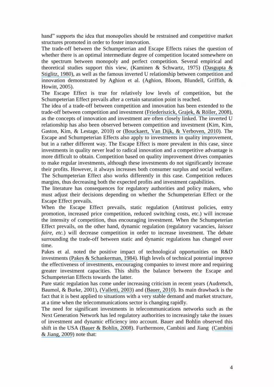
Given the assumption of a symmetrical market, the margin (profit per customer)

equals the transportation cost: tii

The relationship between investments and margins is as follows:

When the margin is low, i.e. *It , companies do not make enough profits to invest *I , so they invest tI .

When investment capabilities are high enough, i.e. *It , companies invest *I .

The following graph (figure 2) illustrates the relationship

Figure 2: Investment according to the margin I(t)

The drop in investment for low margin is due to budgetary restrictions. This decrease

in investment is empirically observed in the next section.

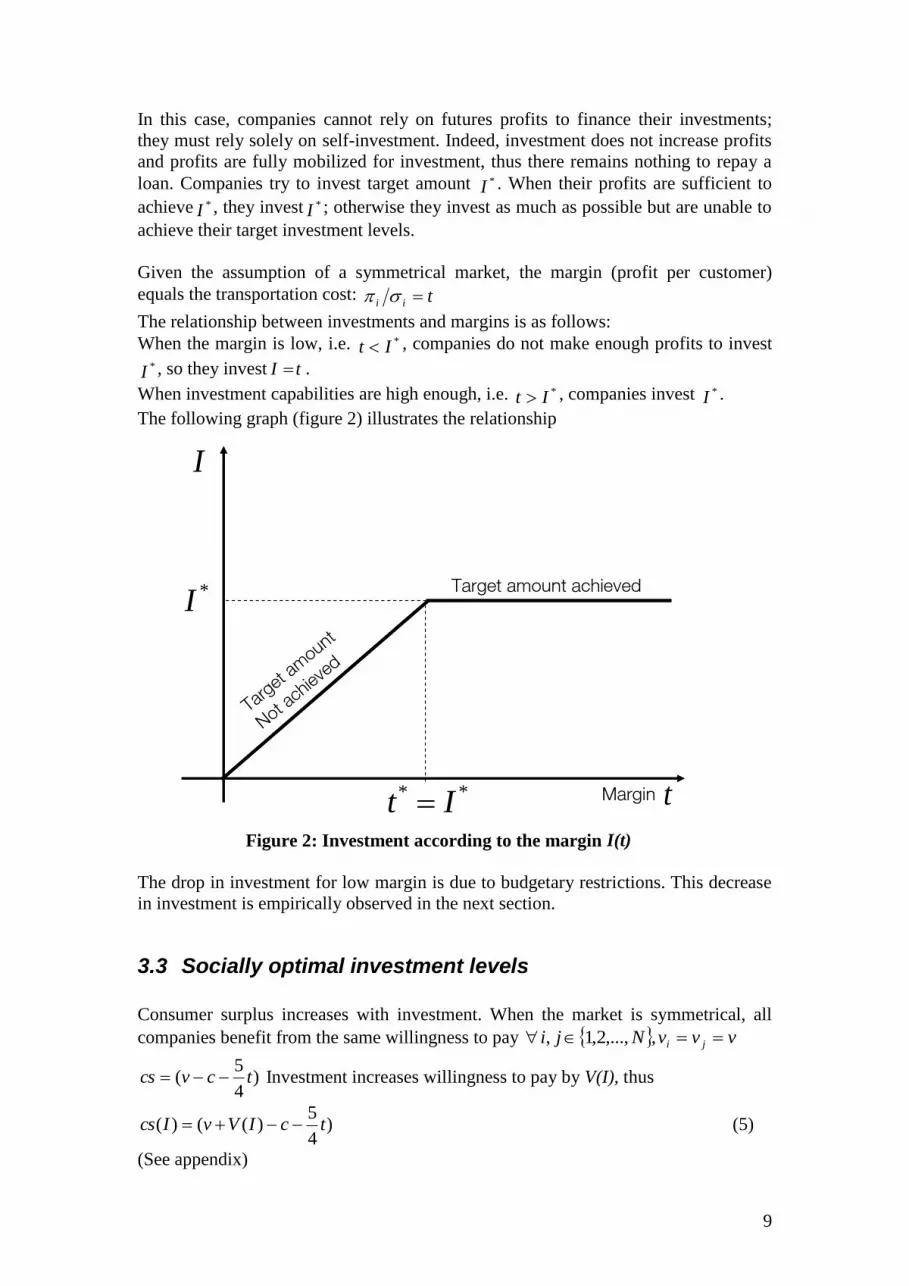
3.3 Socially optimal investment levels

Consumer surplus increases with investment. When the market is symmetrical, all

companies benefit from the same willingness to pay vvvNji ji ,,...,2,1,

)4

5( tcvcs Investment increases willingness to pay by V(I), thus

)4

5)(()( tcIVvIcs (5)

(See appendix)

*I

I

t

Target amount achieved

Target

am

ount

Not ach

ieved

Margin** It

10

and as a result )()( IVcsIcs

Social Welfare, defined as the sum of consumer surplus and total profits generated on

the market, is written as: )()()( IIcsIw

The market size is normalized to 1, so the profit generated on the market is

)1()( ItI . The market’s symmetry encourages all companies to invest the

same amount and prevents them from winning a competitive advantage. Investment

ultimately increases consumer surplus but decreases corporate profits. What level of

investment **I maximizes welfare?

Welfare is written as:

)1()4

)(()( It

cIVvIw (6)

The first order condition leads to the following equation:

)1()( **

dI

IdV (7)

A comparison of equations 4 and 7 shows that dIIdVdIIdV )()( *** . As a result, *** II . The socially optimal level of investment is always greater than the

investment level which maximizes corporate profits. As we saw in subsection 3.2,

companies are never encouraged to exceed the target level , meaning that they always

invest less than the socially optimal level **I . They come closest to achieving **I when they can afford to invest *I .

3.4 Socially optimal margins

Equations (5) and (6) represent consumer surplus and welfare according to the margin

t (figure 3).

Figure 3: Optimal margin which maximizes consumer surplus and welfare3

3 The graph is based on the assumption that the impact of investment on consumers is high enough that

45)( * dIIdV . Consumer surplus and welfare increase as long as *tt

t** It

Surplus

)(tcs

)(tw

cvmargin

11

Derivatives of equations (5) and (6) provide variations of consumer surplus and

welfare according to t:

4

5

dt

dI

dI

dV

dt

dcs and )1(

4

1

dt

dI

dt

dI

dI

dV

dt

dw

Figure 2 indicates that investment depends on whether the value of the margin is

lower or higher than the target level. If *It , then tI and 1dtdI . If *It then *II and 0dtdI .

If *It , 4

5

dI

dV

dt

dcs and

4

5

dI

dV

dt

dw, any margin growth is used to invest.

As long as the impact of investment on consumers is high enough, and so as long as

the dynamic effects outweigh the static effects: ( 45dIdV for consumer surplus

and 45dIdV for welfare), the margin’s growth increases both consumer

surplus and welfare.

If *It 45dtdcs and 41dtdw , however, the margin’s growth is no

longer used to make investments. The dynamic effects disappear, leaving only static

effects, so both consumer surplus and welfare decrease with the margin.

When the dynamic effects are high enough ( 45dIdV for consumer surplus and

45dIdV for welfare), the margin values which maximize consumer surplus

or welfare are both strictly positive. The socially optimal margin value is therefore not

equal to zero. The socially optimal situation is not perfect competition. A certain

degree of margin t, which reduces market fluidity, can be socially efficient.

The greater the potential for technical progress, the higher the socially optimal margin

value.

Moreover, if 23N , then 45)( * dIIdV , and consumer surplus and

welfare are maximum for the same value ** Itt (case of figure 3).

Remark: Investment mainly benefits the telecommunications sector and equipment

suppliers. If we consider welfare without investment, equation (6) becomes:

)4

)(()(t

cIVvIw . In that case, welfare is always maximum when ** Itt .

Quality improvement based competition can be characterized by the target amount of

investment *I and price-based competition by the level of margin t or rather by t1 ,

the level of substitutability.

Maximum welfare occurs for 1* tI which means that the level of quality

improvement based competition is inversely proportional to the level of price-based

competition.

12

4 Empirical analysis

This section provides an empirical analysis of the relationship between investment

and margin per user for in wireless markets in 30 countries between 2002 and 2010. It

highlights the existence of a breaking point in the relationship between margin and

investment. Companies’ investment behavior in a country tends to change when their

margins reach a certain threshold. Below the threshold, investment increases sharply

with the margin, while the increase is slower above the threshold. The theoretical

model in the previous section predicts this type of change in a symmetrical and fully

covered market (figure 2). In that specific case, beyond the threshold (the target

level), growth in investment is nil.

Section 3 address the problem in terms of the firms problem, however, because the

market is assumed to be symmetrical, all firms play the same role. As a result the

industry behavior is totally defined by a representative firm. In this section, the

analysis is conducted at the industry level and the results could be compared at the

theoretical results of section 3.

In markets which are not fully covered, investment may increase the number of

consumers and profits. The observed growth of investment, although relatively low,

therefore remains positive. The model also underscores the role of other factors

including market structure, level of service adoption, level of technology and standard

of living.

4.1 Data set

The data set used here is a panel data set for 30 countries (cf. list in appendix, which

includes annual data by country from 2002 to 2010. The data set should comprise 270

observations, however 29 observations are unavailable. The data set therefore

comprises 241 observations. The financial figures used (Revenue, Capex, Ebitda,

HHI and the number of companies) are drawn from the Informa “World Cellular

Information Service”. The number of wireless users, the population and the level of

technology come from the strategy analytics report “Broadband cellular user forecasts

2011-2016 (September 2011)”4, while the standard of living (GNI per Capita) is taken

from the World Bank. A table of descriptive statistics is provided in the appendix.

The dependant variable in the linear regression model is the yearly Capex per user by

country, CAPU in US $. Capex per user is a proxy of investment.

There are two categories of explanatory variables: financial figures, which depend on

the wireless market in the country, and country figures, which are based on the

specificities of each country. A time trend is included, YEAR, which indicates the

number of years counting from 2001, (the value of year in 2002 is 2, and in 2003 is 3,

etc.), as is a squared time trend. Descriptive statistics are available in the appendix

These variables are presented as follows:

4.1.1 Financial figures:

These variables aim to evaluate the market’s impact on investment incentives. First,

the margin per user, MAPU, defined as annual Ebitda divided by the number of users.

4 This report provides not only forecast data but also data from 2002 to 2010.

13

Second, the number of companies on the market, N. Third, the asymmetry index ,

which measures the degree of asymmetry among companies present on the market:

IOA. This index is calculated as follows: 1

1)(

N

HHINIOA . IOA may range from 0

to 1. In a perfectly symmetrical market, IOA=0; IOA increases with market’s

asymmetry. HHI, the Herfindahl index, is expressed as a percentage. When the market

is absolutely symmetrical, all companies have an equal market share: NHHI 1 ,

thus 0IOA . When the market is absolutely asymmetrical, it tends towards a

monopoly; HHI tends towards 1, so IOA tends towards 1 as well. Fourth, the potential

for market growth, PMG. PMG depends on the penetration rate q, defined as the

number of users divided by the total population of the country. Assuming that the

demand function, which expresses the penetration rate according to price, is sigmoid

shaped, which is a common assumption in telecommunications (Fildes and Kumar

2002) potential for market growth is close to its maximum at the middle of market

coverage. When q is low or high, close to 0 or 1, the potential for market growth is

low. )1( qqPMG . The potential for market growth increases with PMG, which

seems more relevant than simply q. The strength of competition is given by COMP,

which is defined by 1-L, where L is the Lerner index. The Lerner index is calculated

yearly by country; it is defined as Ebitda divided by total Revenue on the market.

4.1.2 Country-specific figures:

These variables aim to take into account the specific situation of each country. First,

the density of population, DPOP, defined as the total population divided by the

country’s surface area. Density may have an impact on investment. Second, the

standard of living, given by the Gross National Income per capita, GNICAP,

expressed in PPP. Finally, the level of technical advances integrated in the network,

3GT, defined as the proportion of subscriptions using 3G technologies as CDMA

2000, WCDMA or LTE.

The following table (Table 1) represents the descriptive statistics of the variables.

CAPU MAPU COMP N IOA PMG 3G DPOP YEAR GNICAP

Mean 62,24 172,61 60,72% 5,94 14,50% 18,13% 14,88% 564 5,33 26579

Standard error 2,10 5,78 0,69% 0,60 0,69% 0,26% 1,29% 102 0,16 810

Median 60,99 173,55 61,33% 4,00 12,38% 17,20% 5,29% 108 5,00 29893

Standard deviation 32,58 89,79 10,76% 9,25 10,76% 3,97% 20,05% 1582 2,45 12575

Variance 1061,57 8061,65 1,16% 85,65 1,16% 0,16% 4,02% 2501646 6,01 158135179

Kurstosis coefficient (flattening) 3,12 -0,24 0,94 38,21 1,43 -1,16 2,58 9,41 -1,11 -0,41

Skewness 1,31 0,44 -0,36 6,05 1,27 0,29 1,67 3,35 -0,12 0,07

Minimum 5,32 12,92 23,76% 2 0,05% 9,35% 0,00% 2,65 1 4064

Maximum 211,11 466,51 93,43% 71 51,99% 25,00% 95,38% 6812,24 9 68547

Sum 15000 41599 146 1432 35 44 36 135976 1285 6405424

Observations 241 241 241 241 241 241 241 241 241 241 Table 1: Descriptive statistics

4.2 Econometric Model

We estimate first the determinants of the margin and we discuss the impact of

investment on future margin. We have shown in section 3 that in a symmetrical and

fully covered market, investment did not increase the margin. However, since markets

are neither perfectly symmetrical nor fully covered, we will see to what extend

investments actually affect margin.

14

4.2.1 Margin equation

We use a panel data regression OLS in order to estimate the coefficients of the

following equation:

iyiykiyjiy YXMAPU (8)

where iyX represents the control variables and iyY the investment variables

iyiyiyiyiyiyiy YEARIOANGNICAPDPOPCOMPX ,,,,, ,

iyiyiyiyiy IOACAPUPMGCAPUCAPUCAPUY *1,*1,1, and iy is the error

term.

CAPU-1 is the Capex per user CAPU lagged one year. CAPU-1*PMG and CAPU-

1*IOA are the lagged values of CAPU multiplied respectively by the Potential for

market growth PMG and index of asymmetry IOA. These variables aim to assess the

impact of the remoteness of assumption of symmetry and full coverage on the margin.

The subscripts of the variables denote country i at year y. The results are presented in

the following table (Table 2):

VARIABLES MAPU (1) MAPU (2) MAPU (3) MAPU (4) MAPU (5) MAPU (6) MAPU (7)

COMP -195.1*** -182.2*** -182.3*** -183.9*** -184.9*** -181.9*** -184.1***

(25.13) (25.86) (24.03) (24.59) (24.41) (24.84) (24.67)

DPOP 0.0755*** 0.0812*** 0.0716*** 0.0807*** 0.0748*** 0.0806*** 0.0804***

(0.0254) (0.0255) (0.0241) (0.0239) (0.0240) (0.0242) (0.0240)

GNICAP 0.00458*** 0.00489*** 0.00426*** 0.00455*** 0.00450*** 0.00461*** 0.00399***

(0.000873) (0.000885) (0.000832) (0.000835) (0.000829) (0.000844) (0.000871)

N 0.0148 -0.288 -0.153 -0.525* -0.581** -0.483* -0.656**

(0.288) (0.276) (0.278) (0.267) (0.266) (0.272) (0.286)

YEAR -0.0121 -2.364* -0.109 -2.684** -2.579** -2.171* -1.837

(1.220) (1.255) (1.162) (1.189) (1.181) (1.211) (1.215)

CAPU 0.0449 0.223** 0.171*

(0.0740) (0.0913) (0.0902)

CAPU-1 0.0374 0.277*** 0.253***

(0.0687) (0.0924) (0.0926)

CAPU-1*PMG 1.127**

(0.497)

CAPU-1*IOA 1.216***

(0.428)

Constant 124.0*** 121.6*** 117.5*** 120.5*** 116.6*** 119.3*** 139.0***

(27.16) (27.59) (26.06) (26.29) (26.18) (26.66) (26.75)

Observations 241 211 238 208 208 208 208

R-squared 0.433 0.384 0.428 0.408 0.420 0.395 0.405

Number of Countries 30 30 30 30 30 30 30

Standard errors in parentheses

*** p<0.01, ** p<0.05, * p<0.1 Table 2: Margin equation

The first specification is the regression on the full sample (241 observations). The

second specification represents the same model with lagged CAPU, that is why we

lose 30 observations (one per country). The results of the second specification are

15

very similar to the first. In this case, Investment seems to have no significant impact

on margin. However, three observations show an abnormally high Capex. For those

observations, Capex is significantly higher than margin. It is possible that these Capex

do not only represent investments in improving quality or that these values are

incorrect. Anyway, in the following columns, we removed these three values leaving

238 observations for CAPU and 208 for CAPU-1. In the third and the fourth

specification, investment has a significant impact on margin. There is no significant

difference between the coefficients estimated in these two specifications which

suggest that an investment remains relatively steady over time. The fifth specification

provides both CAPU and CAPU-1 in order to compare the respective impact of past

year and current year investment on margin. As expected, although both CAPU and

CAPU-1 are significant, the impact of past year is higher and more significant.

Consequently, in the following model, we chose the lagged values of investment

CAPU-1 rather than CAPU. In the sixth specification we replaced CAPU-1 by the

product CAPU-1*PMG and in the seventh we replaced CAPU-1 by the product

CAPU-1*IOA. These variables indicate respectively the impact of the Potential for

Market Growth PMG and the asymmetry of the market on the relationship between

investment and margin. These two variables have a positive and significant impact on

margin. This means that PMG and IOA both increase the impact of investment on

margin. This is consistent with section 3 and the hypothesis of market symmetry and

full coverage. Under such hypothesis, PMG = IOA = 0, Investment has no impact on

margin. Therefore, the impact we highlighted is caused by the fact that markets are

neither fully covered nor symmetrical, even though they often approach close to

symmetry and full coverage. PMG increases profits and thus encourages investment.

Indeed, when PMG is high, investment in quality improvement encourages customers

who were not yet in the market to enter. This increases the market size and thus

profits. Asymmetry of market also encourages investment because asymmetry means

there are leader firms, and leader firms can expect their investment to provide them a

competitive advantage and increase their profits.

The coefficients of control variables are robust to the different specifications. As

expected, competition COMP and the number of firms N have a negative impact on

margin. The density of the population DPOP and the GNI per capita have a positive

one. The time trend YEAR, indicates a decline of margin over time.

4.2.2 Investment equation

The investment equation emphasizes the difference in behavior between companies

according to their margins. In order to do so, we will compare two hypotheses: The

first hypothesis, H0 supposes there is no change in firms’ behavior according to their

margin. The corresponding equation is as follow:

iyiyyi MAPUCAPU 10 (9)

The Capex per user CAPU is explained by the margin per user MAPU. is the error

term.

The alternative hypothesis, Ha supposes there is a break in firms’ behavior. Before the

break, for the low values of margin, Capex per user follows the equation (9) and after

the break, Capex per users follows the following equation:

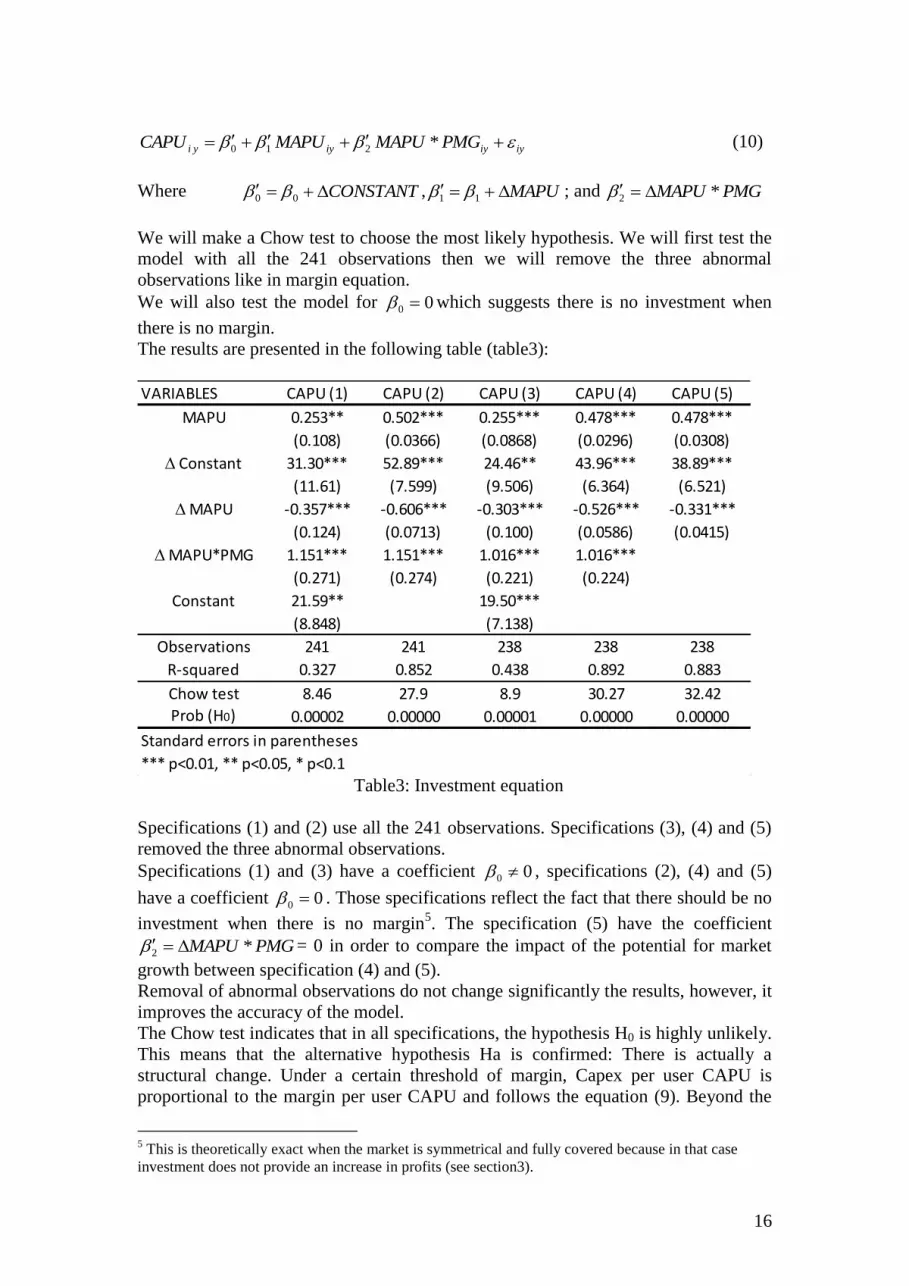
16

iyiyiyyi PMGMAPUMAPUCAPU *210 (10)

Where CONSTANT 00 , MAPU 11 ; and PMGMAPU *2

We will make a Chow test to choose the most likely hypothesis. We will first test the

model with all the 241 observations then we will remove the three abnormal

observations like in margin equation.

We will also test the model for 00 which suggests there is no investment when

there is no margin.

The results are presented in the following table (table3):

VARIABLES CAPU (1) CAPU (2) CAPU (3) CAPU (4) CAPU (5)

MAPU 0.253** 0.502*** 0.255*** 0.478*** 0.478***

(0.108) (0.0366) (0.0868) (0.0296) (0.0308)

Constant 31.30*** 52.89*** 24.46** 43.96*** 38.89***

(11.61) (7.599) (9.506) (6.364) (6.521)

MAPU -0.357*** -0.606*** -0.303*** -0.526*** -0.331***

(0.124) (0.0713) (0.100) (0.0586) (0.0415)

MAPU*PMG 1.151*** 1.151*** 1.016*** 1.016***

(0.271) (0.274) (0.221) (0.224)

Constant 21.59** 19.50***

(8.848) (7.138)

Observations 241 241 238 238 238

R-squared 0.327 0.852 0.438 0.892 0.883

Chow test 8.46 27.9 8.9 30.27 32.42

Prob (H0) 0.00002 0.00000 0.00001 0.00000 0.00000

Standard errors in parentheses

*** p<0.01, ** p<0.05, * p<0.1 Table3: Investment equation

Specifications (1) and (2) use all the 241 observations. Specifications (3), (4) and (5)

removed the three abnormal observations.

Specifications (1) and (3) have a coefficient 00 , specifications (2), (4) and (5)

have a coefficient 00 . Those specifications reflect the fact that there should be no

investment when there is no margin5. The specification (5) have the coefficient

PMGMAPU *2 = 0 in order to compare the impact of the potential for market

growth between specification (4) and (5).

Removal of abnormal observations do not change significantly the results, however, it

improves the accuracy of the model.

The Chow test indicates that in all specifications, the hypothesis H0 is highly unlikely.

This means that the alternative hypothesis Ha is confirmed: There is actually a

structural change. Under a certain threshold of margin, Capex per user CAPU is

proportional to the margin per user CAPU and follows the equation (9). Beyond the

5 This is theoretically exact when the market is symmetrical and fully covered because in that case

investment does not provide an increase in profits (see section3).

17

threshold, CAPU follows the equation (10). The margin threshold is chosen for the

value of MAPU that maximizes the fisher’s statistic of the chow test. This occurs for a

value of MAPU=117 $/user/year.

Equation (10) does not depend on the initial specification of the coefficient 0 . We

can notice that CONSTANT 00 and MAPU 11 have exactly the same

values in specification (1) and (2) and in specification (3) and (4).

The structural change in investment behavior according to the margin is consistent

with the theoretical framework of section 3.

For low margin values (under the threshold), the target amount of investment is not

achieved, therefore an increase in margin entails a proportional increase in investment

to approach the target amount.

For high values of margin (above the threshold), the target amount is achieved and an

increase in margin does not necessary lead to a higher investment. The value of

MAPU 11 in specifications (2), where 104.0606.0505.01 and in

specification (4), where 048.0526.0478.01 , is very low (and negative),

barely significant in specification (2) and not significant in specification (4). Only the

specification (5) indicates a positive and significant coefficient

147.0331.0478.01 but this is just because we do not have taken into account

the variable PMGMAPU * . In specifications (2) and (4), the coefficient of this

variable, 2 , is positive and significant. This variable, indeed, captures all the impact

of the variation of the margin. This means that, beyond the threshold, the impact of

margin on investment is positive only if the Potential for market growth, PMG, is

nonzero. As a result, when the market is fully covered, the margin has no impact on

investment, as theoretically stated in section 3. However, when the potential for

market growth is high, investment increases the market size and future profits, as

shown in the margin equation. Thereby, an increase in margin leads to an increase in

investment.

The figure below (figure.4) illustrates the relationship between margin and

investment.

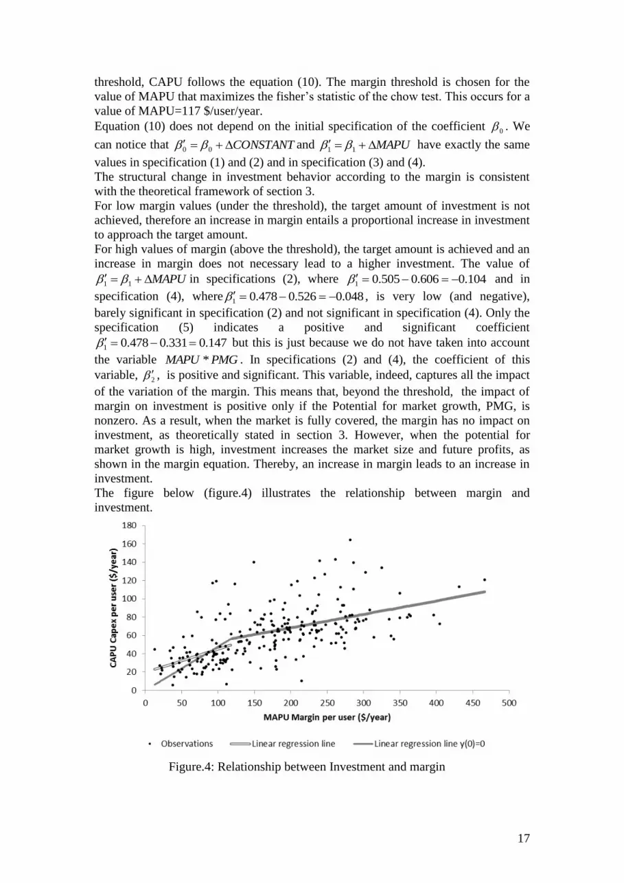
Figure.4: Relationship between Investment and margin

18

The linear regression lines on Figure 4, calculated when the 3 abnormal observations

are removed, are quite similar to the theoretical Figure 2. Especially the “y (0) = 0”

line where 00 . The break between low margin and high margin values appears

clearly from both sides of the margin threshold (MAPU=117 $/year). The main

difference is the slope of the line due to the potential for market growth. It is

noteworthy that when 00 (y (0) =0 line), the two half-lines are continuous at the

breaking point. This is not the case when 00 . Thus the hypothesis 00 is

consistent with the trend beyond the threshold. The fact that markets are neither fully

covered nor perfectly symmetrical could explain the constant.

Investment behavior is different from either sides of the breaking threshold. Before

the breaking threshold, margin is too low to achieve the target amount of investment.

Thereby, in this case, an increase in margin results in a proportional increase in

investment in order to approach the target amount. Beyond the breaking threshold, the

target amount is achieved. An increase in margin does not result in an increase in

investment if the market is not fully covered. When the market is fully covered, the

target amount is achieved and the investment is no more linked to the margin as

indicated by equation 4 in the theoretical framework. When the market is not fully

covered, target amount depends on the margin. An increase in investment allows an

increase in market size and profits, and therefore, margin is reinvested proportionally

to the potential for market growth.

4.2.3 Impact of competition on investment

Considering that beyond the margin threshold the target amount is achieved,

investment does not exceed this target amount. As a result, we consider that, in such

case, CAPU equals the target amount. We will now test the impact of the other

variables: (COMP, N and 3G+) on the target amount. Beyond the threshold

MAPU>117 $/year,

iyiyyi XCAPU 0 (11)

With X, the vector of variables GNCOMPPMGMAPUMAPUX 3,,,*, , and

the coefficients to be estimated. The results are presented in the following table

(Table.4) VARIABLES CAPU (1) CAPU (2) CAPU (3) CAPU (4)

COMP 58.16*** 39.43** 49.15*** 35.18***

(21.45) (17.36) (9.826) (8.036)

N 2.833*** 2.760*** 2.758*** 2.724***

(0.714) (0.574) (0.694) (0.558)

3G+ 26.65*** 33.62*** 27.88*** 34.21***

(9.698) (7.829) (9.319) (7.515)

MAPU -0.0177 0.0129 -0.0332 0.00564

(0.0659) (0.0532) (0.0571) (0.0461)

MAPU*PMG 0.844*** 0.776*** 0.872*** 0.789***

(0.299) (0.240) (0.292) (0.235)

Constant -7.950 -3.743

(16.81) (13.53)

Observations 158 156 158 156

R-squared 0.357 0.477 0.914 0.941

Standard errors in parentheses

*** p<0.01, ** p<0.05, * p<0.1 Table.4: Target amount of investment

19

Specifications (1) and (3) use all the 241 observations, specifications (2) and (3)

removed the three abnormal observations. Specifications (1) and (2) use the constant

term while specifications (3) and (4) do not.

Coefficients of competition COMP and number of firms N are positive and significant

in all the specifications in table 4.

Competition has an ambiguous impact on investment. On the one hand, table 4

indicates that competition tends to increase; however, on the other hand, table 2

highlights that competition decreases margin.

The overall impact of competition on target amount seems to be positive provided the

potential for market growth is not too high, because the variable MAPU, as in

equation 10, is not significant. Although variable MAPU*PMG is positive and

significant, its impact becomes negligible when market approach the full coverage.

However, when competition is fierce enough to reduce the margin below the

threshold, then the target amount is no more achieved. In this case, margin is pushed

below the threshold where investment is proportional to the margin. As a result,

investment decreases.

In other words, competition has a positive impact on investment as long as the target

amount can be reached; otherwise it has a negative impact.

4.2.4 Discussion

As we discussed in subsection 3.3, the target investment level is lower than the

socially optimal level of investment, but is the highest amount that companies are

encouraged to invest. Non-achievement of the target level thus means

underinvestment and a decrease in consumer surplus and social welfare. A low

margin may cause non-achievement of the target investment level. This could explain

the inverted U relationship between investment and competition. As we have seen,

competition and the number of companies have a positive impact on investment when

the margin is sufficient to achieve the target investment level. However, they also

have a negative impact on the margin. If this negative impact is strong enough to

decrease the margin to a point below the level which makes it possible to achieve the

target investment level, the overall impact may be negative. Otherwise the overall

impact remains positive.

5 Conclusion and policy implications

Competition based on quality improvement leads to a target investment level which

companies strive to achieve in order to maximize their profits. This target level is

lower than the socially optimal level, meaning that the target level is, in social terms,

the best level of investment that companies are encouraged to make. However,

companies need to have adequate margins to achieve their target amounts. A lack of

resources causes non-achievement of the target level and entails a decrease in

technical progress, consumer surplus and welfare.

The potential for technical progress increases investment’s impact on quality. The

target level is thus even higher than the potential for technical progress. This potential

is particularly high for information technologies and telecommunications, meaning

20

that the target investment level is particularly high and difficult to achieve. There are

many examples where the target level is not achieved, not only in emerging countries

where standards of living are low, but also in developed countries when price-based

competition is too fierce.

There is a trade-off between competition based on quality improvement, which

represents the dynamic side of competition, and competition based on pricing, which

represents the static side of competition. These two types of competition can be seen

as competitors. Welfare is maximized when the target investment level is exactly

achieved. For a given potential for technical progress providing a given target

investment level and thus a given level of dynamic competition, the static side of

competition should be adjusted in order to allow achievement of the target level.

Regulatory and competition authorities in the sector should avoid underinvestment by

ensuring that companies are able to achieve their target levels.

In terms of market tools, competition and entry have a positive impact on investment

but only when companies can achieve their target levels, otherwise they may have a

negative impact.

Appendix

List of countries:

Argentina 2004-2010; Australia 2005-2010; Austria 2002-2010; Belgium 2003-2010;

Brazil 2002-2010; Canada 2002-2010; China 2005-2010; Colombia 2005-2010; Egypt

2006-2010; France 2003-2010; Germany 2002-2010; Hong-Kong 2002-2010;

Hungary 2002-2010; Italy 2002-2010; Japan 2004-2010; Korea 2002-2010; Mexico

2003-2010; Netherland 2003-2010; Norway 2002-2010; Poland 2002-2010; Portugal

2002-2010; Russia 2002-2010; Singapore 2003-2010; South Africa 2002-2010; Spain

2004-2010; Sweden 2002-2010; Switzerland 2003-2008; Turkey 2003-2010; UK

2002-2010; USA 2002-2010.

Correlation Matrix:

Correlation matrix CAPU MAPU COMP NF IOA PMG 3GT DPOP YEAR GNICAP

CAPU 1.000

MAPU 0.505 1.000

COMP 0.003 -0.314 1,000

NF 0.119 -0.166 -0.087 1.000

IOA -0.068 -0.192 -0.155 0.190 1.000

PMG -0.114 -0.307 -0.027 0.096 0.416 1.000

3GT 0.324 0.363 0.142 -0.119 -0.139 -0;443 1.000

DPOP -0.021 -0.038 0.138 -0.050 -0.211 -0.352 0.119 1.000

YEAR -0.084 0.075 0.033 -0.153 -0.021 -0.311 0.609 -0.002 1.000

GNICAP 0.469 0.783 0.069 -0.148 -0.376 -0.457 0.447 0.227 0.136 1.000

Proof of equation (4):

)1(1

12

)()()1(

12

)1(2

NN

IVIVN

tdI

dV

N

N

NtdI

d ji

ji

ii

i

21

If the market is symmetrical, III ji ; in that case,

ji

ji IVIVN )()()1( and

therefore: )1(1)(

12

)1(2

NdI

IdV

N

N

NdI

d

ii

i

The first order condition 0

dI

d

dI

d i

i

i leads to

)1(2

)12)(1()( *

N

N

dI

IdV equation (4)

Proof of equation (5) and (6):

There are N spokes and

2

)1( NN different i,j pairs. There are Nq consumers on

each spoke or Nq2 customer for each pair. Each company appears in 1N pairs.

Let us denote ijcs the consumer surplus of the pair i,j. Total Consumer surplus is:

ijij cscsNN

NNcs

)1(

12

2

)1(

1

0 ij

ij

x

j

x

iij dxUdxUcs

When market is symmetrical, vvv ji ; 21ijx

)4

5()2()(

1

21

21

0

tcvdxtxtcvdxtxtcvqcscs ij

Welfare is the sum of consumer surplus and industry profits.

In a symmetrical market, industry profits are )1( Itq . Welfare is written:

)1()4

1( Itcvw

Bibliography:

Aghion, P., Bloom, N., Blundell, R., Griffith, R., & Howitt, P. (2005). Competition

and Innovation: An Inverted-U Relationship*. Quarterly Journal of

Economics, 120(2), 701–728.

Audretsch, D. B., Baumol, W. J., & Burke, A. E. (2001). Competition policy in

dynamic markets. International Journal of Industrial Organization, 19(5),

613–634.

22

Bauer, J. M. (2010). Regulation, public policy, and investment in communications

infrastructure. Telecommunications Policy, 34(1-2), 65–79.

Bauer, J. M., & Bohlin, E. (2008). From Static to Dynamic Regulation.

Intereconomics, 43(1), 38–50.

Bouckaert, J., Van Dijk, T., & Verboven, F. (2010). Access regulation, competition,

and broadband penetration: An international study. Telecommunications

Policy, 34(11), 661–671.

Cambini, C., & Jiang, Y. (2009). Broadband investment and regulation: A literature

review. Telecommunications Policy, 33(10-11), 559–574.

Chen, Y., & Riordan, M. H. (2007). Price and Variety in the Spokes Model*. The

Economic Journal, 117(522), 897–921.

Dasgupta, P., & Stiglitz, J. (1980). Industrial structure and the nature of innovative

activity. The Economic Journal, 90(358), 266–293.

Fildes, R., & Kumar, V. (2002). Telecommunications demand forecasting---a review.

International Journal of Forecasting, 18(4), 489--522.

Friederiszick, H., Grajek, M., & Röller, L. H. (2008). Analyzing the relationship

between regulation and investment in the telecom sector. ESMT White Paper

WP-108-01.

Gilbert, R. J., & Newbery, D. M. . (1982). Preemptive patenting and the persistence of

monopoly. The American Economic Review, 72(3), 514–526.

Jeanjean, F.; , "Competition through Technical Progress," Telecommunication, Media

and Internet Techno-Economics (CTTE), 10th Conference of , vol., no., pp.1-

15, 16-18 May 2011

Kaminen, M., & Schwartz, N. (1975). Market structure and innovation: a survey. The

Journal of Economics Literature.

23

Kim, J., Kim, Y., Gaston, N., Kim, Y., & Lestage, R. (2010). Access regulation,

competition, and the investment of network operators in the mobile

telecommunications industry. Globalisation and Development Centre, 34.

Loury, G. C. (1979). Market structure and innovation. The Quarterly Journal of

Economics, 395–410.

Pakes, A., & Schankerman, M. (1984). An exploration into the determinants of

research intensity. University of Chicago Press.

Reichl, P., Tuffin, B., & Schatz, R. (2010). Economics of logarithmic Quality-of-

Experience in communication networks. Telecommunications Internet and

Media Techno Economics (CTTE), 2010 9th Conference on (p. 1–8).

Salop, S. C. (1979). Monopolistic competition with outside goods. The Bell Journal of

Economics, 10(1), 141–156.

Schumpeter, J. A. (1942). Socialism, capitalism and democracy. Harper and Bros.

Sutton, J. (1991). Sunk costs and market structure: Price competition, advertising,

and the evolution of concentration. The MIT press.

Valletti, T. M. (2003). The theory of access pricing and its linkage with investment

incentives. Telecommunications Policy, 27(10-11), 659–675.