improving portfolio selection using option-implied volatility and skewness
TRANSCRIPT

JOURNAL OF FINANCIAL AND QUANTITATIVE ANALYSIS Vol. 48, No. 6, Dec. 2013, pp. 1813–1845COPYRIGHT 2013, MICHAEL G. FOSTER SCHOOL OF BUSINESS, UNIVERSITY OF WASHINGTON, SEATTLE, WA 98195doi:10.1017/S0022109013000616
Improving Portfolio Selection UsingOption-Implied Volatility and Skewness
Victor DeMiguel, Yuliya Plyakha, Raman Uppal,and Grigory Vilkov∗
Abstract
Our objective in this paper is to examine whether one can use option-implied informa-tion to improve the selection of mean-variance portfolios with a large number of stocks,and to document which aspects of option-implied information are most useful to improvetheir out-of-sample performance. Portfolio performance is measured in terms of volatil-ity, Sharpe ratio, and turnover. Our empirical evidence shows that using option-impliedvolatility helps to reduce portfolio volatility. Using option-implied correlation does notimprove any of the metrics. Using option-implied volatility, risk premium, and skewnessto adjust expected returns leads to a substantial improvement in the Sharpe ratio, even afterprohibiting short sales and accounting for transaction costs.
I. Introduction
To determine the optimal mean-variance portfolio of an investor, one needs toestimate the moments of asset returns, such as means, volatilities, and correlations.
∗DeMiguel, [email protected], London Business School, 6 Sussex Place, Regent’s Park,London NW1 4SA, United Kingdom; Plyakha, [email protected], Luxembourg School of Finance,University of Luxembourg, 4, rue Albert Borschette, L-1246 Luxembourg; Uppal, [email protected], Edhec Business School, 10 Fleet Place, Ludgate, London EC4M 7RB, United King-dom and Center for Economic and Policy Research (CEPR); and Vilkov, [email protected], GoetheUniversity Frankfurt, Finance Department, Gruneburgplatz 1 / Uni-Pf H 25, Frankfurt am Main,D-60323, Germany. We gratefully acknowledge financial support from INQUIRE-Europe; however,this article represents the views of the authors and not of INQUIRE. We acknowledge detailed feed-back from Luca Benzoni, Massimo Guidolin (the referee), Pascal Maenhout, and Christian Schlag.We received helpful comments and suggestions from Alexander Alekseev, Hendrik Bessembinder(the editor), Michael Brandt, Mike Chernov, Engelbert Dockner, Bernard Dumas, Wayne Ferson,Rene Garcia, Lorenzo Garlappi, Nicolae Garleanu, Amit Goyal, Jakub Jurek, Nikunj Kapadia, RalphKoijen, Lionel Martellini, Vasant Naik, Stavros Panageas, Andrew Patton, Boryana Racheva-Iotova,Marcel Rindisbacher, Paulo Rodrigues, Pedro Santa-Clara, Bernd Scherer, Peter Schotman, GeorgeSkiadopoulos, Luis Viceira, Josef Zechner, and seminar participants at AHL (Man Investments),BlackRock, Goethe University Frankfurt, London School of Economics, University of Mainz, Univer-sity of Piraeus, University of St. Gallen, Vienna University of Economics and Business Administra-tion, CEPR European Summer Symposium on Financial Markets, Duke-University of North Carolinaat Chapel Hill Asset Pricing Conference, EDHEC-Risk Seminar on Advanced Portfolio Construction,Financial Econometrics Conference at Toulouse School of Economics, Stockholm Institute for Finan-cial Research Conference on Asset Allocation and Pricing in Light of the Recent Financial Crisis, andmeetings of the European Finance Association, Western Finance Association, and the Joint Confer-ence of INQUIRE-UK and INQUIRE-Europe 2011.
1813

1814 Journal of Financial and Quantitative Analysis
Traditionally, historical data on returns are used to estimate these moments, butresearchers have found that portfolios based on sample estimates perform poorlyout of sample.1 Several approaches have been proposed for improving the perfor-mance of portfolios based on historical data.2
In this paper, instead of trying to improve the quality of the moments es-timated from historical data, we use forward-looking moments of stock-returndistributions that are implied by option prices. The main contribution of our workis to evaluate empirically which aspects of option-implied information are par-ticularly useful for improving the out-of-sample performance of portfolios witha large number of stocks. Specifically, we consider option-implied volatility, cor-relation, skewness, and the risk premium for stochastic volatility, and we obtainthese not just from the Black-Scholes (1973) model, but also using the model-freeapproach, which has the benefit that the measurement error resulting from modelmisspecification is reduced.
In selecting portfolios, we use a variety of moments implied by prices of op-tions. First, we consider the use of option-implied volatilities and correlations toimprove out-of-sample performance of mean-variance portfolios invested in onlyrisky stocks. When evaluating the benefits of using option-implied volatilities andcorrelations, we set expected returns to be the same across all assets so that theresults are not confounded by the large errors in estimating expected returns.3
Consequently, the mean-variance portfolio reduces to the minimum-variance port-folio. In addition to considering the minimum-variance portfolio based on thesample covariance matrix, we consider also the short-sale-constrained minimum-variance portfolio, the minimum-variance portfolio with shrinkage of the covari-ance matrix (as in Ledoit and Wolf (2004a), (2004b)), and the minimum-varianceportfolio obtained by assuming all correlations are equal to 0 or with correlationsset equal to the mean correlation across all asset pairs (as suggested by Elton,Gruber, and Spitzer (2006)). We find that using risk-premium-corrected option-implied volatilities in minimum-variance portfolios improves the out-of-samplevolatility by more than 10% compared to the traditional portfolios based on onlyhistorical stock-return data, while the changes in the Sharpe ratio are insignifi-cant. Thus, using option-implied volatility allows one to reduce the out-of-sampleportfolio volatility significantly.
Next, we examine the use of risk-premium-corrected option-implied cor-relations to improve the performance of minimum-variance portfolios. We findthat in most cases option-implied correlations do not lead to any improvement
1For evidence of this poor performance, see DeMiguel, Garlappi, and Uppal (2009), Jacobs,Muller, and Weber (2010), and the references therein.
2These approaches include: imposing a factor structure on returns (Chan, Karceski, andLakonishok (1999)), using data for daily rather than monthly returns (Jagannathan and Ma (2003)),using Bayesian methods (Jobson, Korkie, and Ratti (1979), Jorion (1986), Pastor (2000), and Ledoitand Wolf (2004b)), constraining short sales (Jagannathan and Ma), constraining the norm of the vectorof portfolio weights (DeMiguel, Garlappi, Nogales, and Uppal (2009)), and using stock-return char-acteristics such as size, book-to-market ratio, and momentum to choose parametric portfolios (Brandt,Santa-Clara, and Valkanov (2009)).
3Jagannathan and Ma ((2003), pp. 1652–1653) write, “The estimation error in the sample mean isso large nothing much is lost in ignoring the mean altogether when no further information about thepopulation mean is available.”

DeMiguel, Plyakha, Uppal, and Vilkov 1815
in performance. Our empirical results indicate that the gains from using impliedcorrelations are not substantial enough to offset the higher turnover resulting fromthe increased instability over time of the covariance matrix when it is estimatedusing option-implied correlations.
Finally, to improve the out-of-sample performance of mean-variance portfo-lios, we consider the use of option-implied volatility, risk premium for stochasticvolatility, and option-implied skewness. These characteristics have been shownin the literature to help explain the cross section of expected returns.4 Therefore,it makes sense to explore their effect in the framework of mean-variance portfo-lios. Using these characteristics to rank stocks and adjusting by a scaling factor theexpected returns of the stocks, or using these characteristics with the parametric-portfolio methodology of Brandt et al. (2009), leads to a substantial improvementin the Sharpe ratio, even after prohibiting short sales and accounting for transac-tion costs.
We conclude this Introduction by discussing the relation of our work to theexisting literature. The idea that option prices contain information about futuremoments of asset returns has been understood ever since the work of Black andScholes (1973) and Merton (1973); Poon and Granger (2005) provide a compre-hensive survey of this literature. The focus of our work is to investigate how theinformation implied by option prices can be used to improve portfolio selection.Two other papers study this question. The first, by Aıt-Sahalia and Brandt (2008),uses option-implied state prices to solve for the intertemporal consumption andportfolio choice problem using the Cox and Huang (1989) martingale representa-tion formulation rather than the Merton (1971) dynamic-programming formula-tion; however, the focus of the paper is not on finding the optimal portfolio withsuperior out-of-sample performance. The second, by Kostakis, Panigirtzoglou,and Skiadopoulos (2011), studies the asset-allocation problem of allocating wealthbetween the Standard & Poor’s (S&P) 500 index and a riskless asset. That paperfinds that the out-of-sample performance of the portfolio based on the return dis-tribution inferred from option prices is better than that of a portfolio based onthe historical distribution. However, there is an important difference between thatwork and ours: Rather than considering the problem of how to allocate wealthbetween the S&P 500 index and the risk-free asset, we consider the portfolio-selection problem of allocating wealth across a large number of individual stocks.It is not clear how one would extend the methodology of Kostakis et al. to accom-modate a large number of risky assets. They also need to make other restrictiveassumptions, such as the existence of a representative investor and the complete-ness of financial markets, which are not required in our analysis.
The rest of the paper is organized as follows: In Section II, we describe thedata on stocks and options that we use. In Section III, we explain how we use dataon options to predict volatilities, correlations, and expected returns. In Section IV,
4For instance, Bollerslev, Tauchen, and Zhou (2009) document a positive relation between thevariance risk premium and future returns. Bali and Hovakimian (2009) and Goyal and Saretto (2009)show that stocks with a large spread between Black-Scholes (1973) implied volatility and realizedvolatility tend to outperform those with low spreads. Bali and Hovakimian (2009), Xing, Zhang, andZhao (2010), and Cremers and Weinbaum (2010) find a positive relation between various measures ofoption-implied skewness and future stock returns.

1816 Journal of Financial and Quantitative Analysis
we describe the construction of the various portfolios we evaluate along with thebenchmark portfolios, and the metrics used to compare the performance of theseportfolios. Our main findings about the performance of various portfolios that useoption-implied information are given in Section V. We conclude in Section VI.
II. Data
In this section, we describe the data on stocks and stock options that we usein our study. Our data on stocks are from the Center for Research in SecurityPrices (CRSP). To implement the parametric-portfolio methodology, we also usedata from Compustat. Our data for options are from IvyDB (OptionMetrics). Oursample period is from Jan. 1996 to Oct. 2010.5
A. Data on Stock Returns and Stock Characteristics
We study stocks that are in the S&P 500 index at any time during our sampleperiod. The daily stock returns of the S&P 500 constituents are from the daily fileof CRSP, and we have in our sample a total of 3,986 trading days.6 Counting byCRSP identifiers (PERMNO), we have data for a maximum of 961 stocks. Out ofthese 961 stocks, there are 143 stocks for which implied volatilities are availablefor the entire time series. For robustness, we consider two samples in our analysis.The first, which we label “Sample 1,” consists of the 143 stocks for which thereare no missing data. The second, “Sample 2,” consists of all the stocks that arepart of the S&P 500 index on a particular day and that have no missing data onthat day (such as prices of options on the same underlying and the same matu-rity but across different strikes, which are needed to compute model-free impliedvolatility (MFIV) and model-free implied skewness (MFIS)). Thus, the secondsample has a variable number of stocks; on average, there are about 400 stocks ateach date in this sample.7
We measure size (market value of equity) as the price of the stock per sharemultiplied by shares outstanding; both variables are obtained from the CRSPdatabase. For measuring value or book-to-market (BTM) characteristic, we usethe Compustat Quarterly Fundamentals file. The 12-month momentum (MOM)characteristic is measured for each day t using daily returns data from CRSP asthe cumulative return from day t − 251− 21 to day t − 21.8
5We carry out all the tests included in the manuscript also for the pre-crisis period from Jan. 1996to Dec. 2007, and the crisis period from Jan. 2008 to June 2009 (identified as a recession by the Na-tional Bureau of Economic Research (NBER)). The main insights of our analysis do not change withthe choice of sample period. These results are available in the working paper version of the manuscript.
6We also use high-frequency intraday stock-price data consisting of transaction prices for the S&P500 constituents from the NYSE’s Trade and Quote database; the results for these data are very similarto those using daily data.
7The main difference between Sample 1 and Sample 2 is that for estimating the parameters of thecovariance matrix for Sample 2, which has more stocks, one needs a longer estimation window. Thus,while the estimation window for Sample 1 is 250 trading days, for Sample 2 it is 750 days. As a resultof the longer estimation window, the weights are relatively more stable over time for Sample 2. On theother hand, because the covariance matrix for Sample 2 is of a larger dimension, its condition numberis different from that of the covariance matrix for Sample 1.
8To get better distributional properties of the size and BTM characteristics we construct, we takethe logarithm of size and value characteristics. In order to prepare these characteristics so that they

DeMiguel, Plyakha, Uppal, and Vilkov 1817
B. Data on Stock Options
For stock options, we use IvyDB, which contains data on all U.S.-listed indexand equity options, most of which are American. We use the volatility surfacefile, which contains a smoothed implied-volatility surface for a range of standardmaturities and a set of option delta points. From the surface file we select the out-of-the-money implied volatilities for calls and puts (we take implied volatilities forcalls with deltas smaller than or equal to 0.5, and implied volatilities for puts withdeltas bigger than−0.5) for a maturity of 30 days.9 For each date, underlying stock,and time to maturity, we have 13 implied volatilities from the surface data, whichare used to calculate the moments of the risk-neutral distribution. Some of theoption-based characteristics also use the parametric Black-Scholes (1973) impliedvolatilities for at-the-money options. We compute the at-the-money volatility asthe average volatility for a put and a call with absolute delta level equal to 0.5.
III. Option-Implied Information
In this section, we explain how we compute the option-implied moments thatwe use for portfolio selection; we compare the ability of option-implied momentsand the historical moments to forecast the actual realized moments. We considerthe following measures: i) model-free option-implied volatility; ii) the volatilityrisk premium, measured as the spread between realized and Black-Scholes (1973)option-implied volatility; iii) option-implied correlation; iv) model-free option-implied skewness; and v) a proxy for skewness, measured as the spread betweenthe Black-Scholes implied volatility obtained from calls and that from puts.
A. Predicting Volatilities Using Options
When option prices are available, an intuitive first step is to use this infor-mation to back out implied volatilities and use them to predict volatility.10 In con-trast to the model-specific Black and Scholes (1973) implied volatility, we use forthis purpose MFIV, which represents a nonparametric estimate of the risk-neutralexpected stock-return volatility until the option’s expiration. It subsumes infor-mation in the whole Black-Scholes implied volatility smile (Vanden (2008)) andis expected to predict the realized volatility (RV) better than the Black-Scholesvolatility. We compute MFIV as the square root of the variance contract ofBakshi et al. (2003), as explained later.
can be used to compute the parametric-portfolio weights, we also winsorize the characteristics byassigning the value of the 3rd percentile to all values below the 3rd percentile and do the same forvalues higher than the 97th percentile. Finally, we normalize all characteristics to have zero mean andunit standard deviation.
9The use of out-of-the-money options is standard in this literature; see, for instance, Bakshi,Kapadia, and Madan (2003) and Carr and Wu (2009). The reason for selecting options that are outof the money is that it reduces the effect of the premium for early exercise of American options.
10Note that our objective is only to show that the option-implied moments provide better forecaststhan the estimators based on historical sample data, rather than to demonstrate that option-impliedmoments provide the best forecasts of future volatility and correlations. There is a very large literatureon forecasting stock-return volatility and correlations; see, for instance, the survey article by Andersen,Bollerslev, and Diebold (2009).
1818 Journal of Financial and Quantitative Analysis
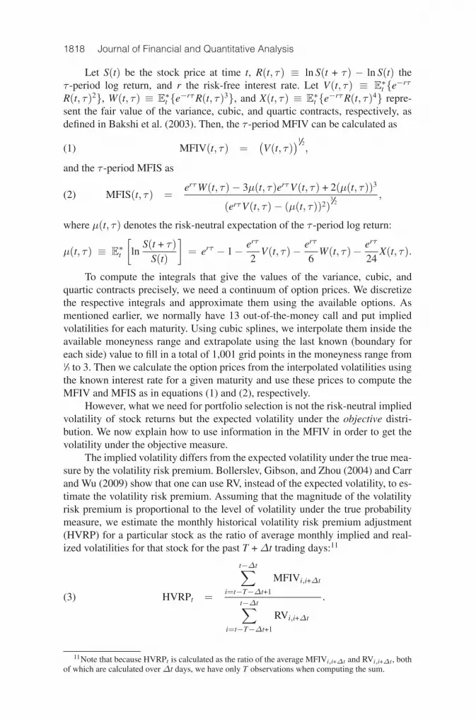
Let S(t) be the stock price at time t, R(t, τ) ≡ ln S(t + τ) − ln S(t) theτ -period log return, and r the risk-free interest rate. Let V(t, τ) ≡ E
∗t {e−rτ
R(t, τ)2}, W(t, τ) ≡ E∗t {e−rτR(t, τ)3}, and X(t, τ) ≡ E
∗t {e−rτR(t, τ)4} repre-
sent the fair value of the variance, cubic, and quartic contracts, respectively, asdefined in Bakshi et al. (2003). Then, the τ -period MFIV can be calculated as
MFIV(t, τ) =(V(t, τ)
)1/2,(1)
and the τ -period MFIS as
MFIS(t, τ) =erτW(t, τ)− 3μ(t, τ)erτV(t, τ) + 2(μ(t, τ))3
(erτV(t, τ)− (μ(t, τ))2)3/2,(2)
where μ(t, τ) denotes the risk-neutral expectation of the τ -period log return:
μ(t, τ) ≡ E∗t
[ln
S(t + τ)S(t)
]= erτ − 1− erτ
2V(t, τ)− erτ
6W(t, τ)− erτ
24X(t, τ).
To compute the integrals that give the values of the variance, cubic, andquartic contracts precisely, we need a continuum of option prices. We discretizethe respective integrals and approximate them using the available options. Asmentioned earlier, we normally have 13 out-of-the-money call and put impliedvolatilities for each maturity. Using cubic splines, we interpolate them inside theavailable moneyness range and extrapolate using the last known (boundary foreach side) value to fill in a total of 1,001 grid points in the moneyness range from1/3 to 3. Then we calculate the option prices from the interpolated volatilities usingthe known interest rate for a given maturity and use these prices to compute theMFIV and MFIS as in equations (1) and (2), respectively.
However, what we need for portfolio selection is not the risk-neutral impliedvolatility of stock returns but the expected volatility under the objective distri-bution. We now explain how to use information in the MFIV in order to get thevolatility under the objective measure.
The implied volatility differs from the expected volatility under the true mea-sure by the volatility risk premium. Bollerslev, Gibson, and Zhou (2004) and Carrand Wu (2009) show that one can use RV, instead of the expected volatility, to es-timate the volatility risk premium. Assuming that the magnitude of the volatilityrisk premium is proportional to the level of volatility under the true probabilitymeasure, we estimate the monthly historical volatility risk premium adjustment(HVRP) for a particular stock as the ratio of average monthly implied and real-ized volatilities for that stock for the past T +Δt trading days:11
HVRPt =
t−Δt∑i=t−T−Δt+1
MFIVi,i+Δt
t−Δt∑i=t−T−Δt+1
RVi,i+Δt
.(3)
11Note that because HVRPt is calculated as the ratio of the average MFIVi,i+Δt and RVi,i+Δt , bothof which are calculated overΔt days, we have only T observations when computing the sum.

DeMiguel, Plyakha, Uppal, and Vilkov 1819
In our analysis, we estimate the HVRP on each day over the past year (−272days to −21 days) using the MFIV and RV from daily returns, each measuredover 21 trading days and each annualized appropriately. Then, assuming that inthe next period, from t to t + Δt, the prevailing volatility risk premium will bewell approximated by the historical volatility risk premium in equation (3), onecan obtain the prediction of the future realized volatility, RVt, which we call therisk-premium-corrected implied volatility:12
RVt,t+Δt =MFIVt,t+Δt
HVRPt.
We now wish to confirm the intuition that risk-premium-corrected impliedvolatility is better than historical volatility at predicting RV. To do this, we con-sider, as a predictor first historical volatility and then risk-premium-corrected im-plied volatility, for the monthly RV from daily returns for each stock. We comparethe performance of each predictor in terms of root mean squared error (RMSE)and mean prediction error (ME). We find that the average RMSE in Sample 1for the risk-premium-corrected implied volatility is 0.1274, which is smaller thanthe RMSE of 0.1671 for historical daily volatility. The ME for both predictors isnegative, indicating that on average both measures are biased upward with respectto the RV; however, the ME of −0.0047 for the risk-premium-corrected impliedvolatility is one order of magnitude smaller than the ME of−0.0185 for historicalvolatility.
B. Predicting Correlations Using Options
The second piece of option-implied information that we consider is impliedcorrelation; because we need the correlation under the objective measure for theportfolio optimization, we discuss directly how to obtain option-implied correla-tion corrected for the risk premium.
If a portfolio is composed of N individual stocks with weights wi,i = {1, . . . ,N}, we can write the variance of the portfolio p under the objective(physical) probability measure P as
(σP
p,t
)2=
N∑i=1
w2i
(σP
i,t
)2+
N∑i=1
N∑j�=i
wiwjσPi,tσ
Pj,tρ
Pij,t.(4)
Assume that we have estimated the expectation of the future volatilities of theportfolio σP
p,t and of its components σPi,t, and we want to estimate the set of ex-
pected correlations ρ Pij,t that turn equation (4) into identity. Once we substitute the
expected volatilities into equation (4) , we have one equation with N×(N − 1) /2unknown correlations, ρ P
ij,t. Thus, to compute all pairwise correlations we need tomake some identifying assumptions.
12Another method for obtaining the predictor of future realized volatility is to use a modified ver-sion of the heterogeneous autoregressive model of RV proposed by Corsi (2009). We find that the rootmean squared error (RMSE) and mean prediction error (ME) with this measure are larger than thoseusing the approach we adopt.
1820 Journal of Financial and Quantitative Analysis
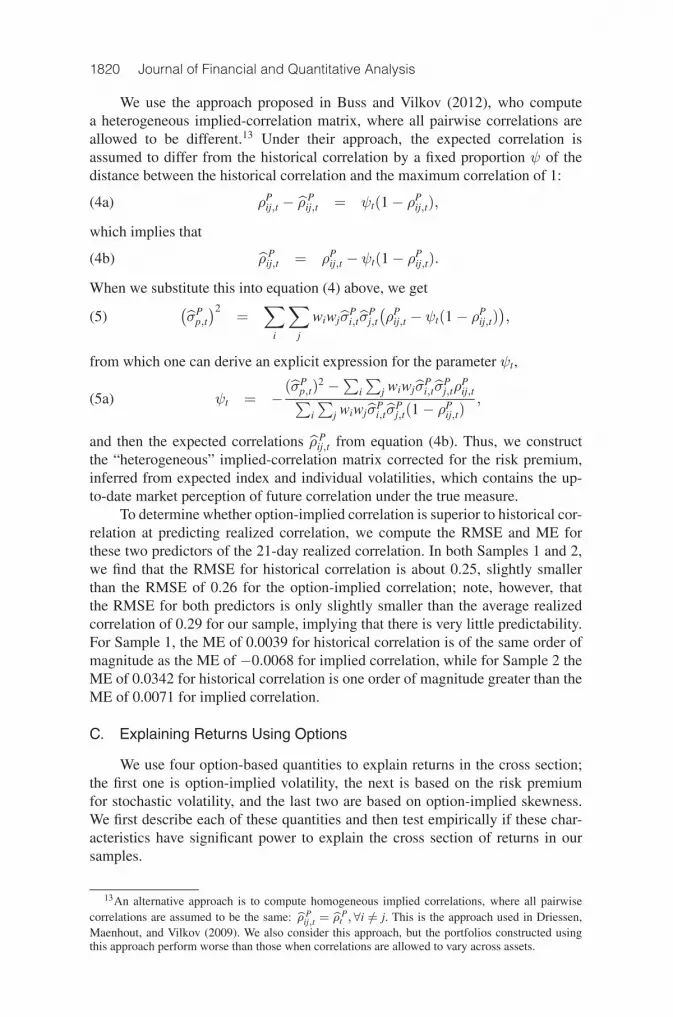
We use the approach proposed in Buss and Vilkov (2012), who computea heterogeneous implied-correlation matrix, where all pairwise correlations areallowed to be different.13 Under their approach, the expected correlation isassumed to differ from the historical correlation by a fixed proportion ψ of thedistance between the historical correlation and the maximum correlation of 1:
ρPij,t − ρ P
ij,t = ψt(1− ρPij,t),(4a)
which implies that
ρ Pij,t = ρP
ij,t − ψt(1− ρPij,t).(4b)
When we substitute this into equation (4) above, we get(σP
p,t
)2=∑
i
∑j
wiwjσPi,tσ
Pj,t
(ρP
ij,t − ψt(1− ρPij,t)),(5)
from which one can derive an explicit expression for the parameter ψt,
ψt = − (σPp,t)
2 −∑i
∑j wiwjσ
Pi,tσ
Pj,tρ
Pij,t∑
i
∑j wiwjσ
Pi,tσ
Pj,t(1− ρP
ij,t),(5a)
and then the expected correlations ρ Pij,t from equation (4b). Thus, we construct
the “heterogeneous” implied-correlation matrix corrected for the risk premium,inferred from expected index and individual volatilities, which contains the up-to-date market perception of future correlation under the true measure.
To determine whether option-implied correlation is superior to historical cor-relation at predicting realized correlation, we compute the RMSE and ME forthese two predictors of the 21-day realized correlation. In both Samples 1 and 2,we find that the RMSE for historical correlation is about 0.25, slightly smallerthan the RMSE of 0.26 for the option-implied correlation; note, however, thatthe RMSE for both predictors is only slightly smaller than the average realizedcorrelation of 0.29 for our sample, implying that there is very little predictability.For Sample 1, the ME of 0.0039 for historical correlation is of the same order ofmagnitude as the ME of −0.0068 for implied correlation, while for Sample 2 theME of 0.0342 for historical correlation is one order of magnitude greater than theME of 0.0071 for implied correlation.
C. Explaining Returns Using Options
We use four option-based quantities to explain returns in the cross section;the first one is option-implied volatility, the next is based on the risk premiumfor stochastic volatility, and the last two are based on option-implied skewness.We first describe each of these quantities and then test empirically if these char-acteristics have significant power to explain the cross section of returns in oursamples.
13An alternative approach is to compute homogeneous implied correlations, where all pairwisecorrelations are assumed to be the same: ρ P
ij,t = ρPt , ∀i =/ j. This is the approach used in Driessen,
Maenhout, and Vilkov (2009). We also consider this approach, but the portfolios constructed usingthis approach perform worse than those when correlations are allowed to vary across assets.

DeMiguel, Plyakha, Uppal, and Vilkov 1821
The first option-based characteristic we use is option-implied volatility. Ang,Bali, and Cakici (2010) show that stocks with high current levels of option-implied volatility earn, in the next periods, higher returns than stocks with lowlevels of implied volatility. To maximize the information content of the option-implied volatility proxy, we use the MFIV described in Section III.A.
The second option-based characteristic we use is the variance risk premium,which is defined as the difference between risk-neutral (implied) and objective(expected or realized) variances. Previous research (see the papers cited in foot-note 4) documents a positive relation between the variance risk premium andfuture stock returns. We use the implied-realized volatility spread (IRVS) as ameasure of the volatility risk premium. We compute IRVS using the approach inBali and Hovakimian (2009) as the spread between the Black-Scholes (1973) im-plied volatility averaged across call and put options and the realized stock-returnvolatility for the past month (21 trading days).
The third characteristic we consider is option-implied skewness, for whichwe use two measures. The first, MFIS, as defined in equation (2), represents anonparametric estimate of the risk-neutral stock-return skewness.14 Rehman andVilkov (2009) find that stocks with high option-implied skewness outperformstocks with low option-implied skewness.15 The second measure of skewnesswe consider is the spread between the Black-Scholes (1973) implied volatilityfor pairs of calls and puts, which is studied in Bali and Hovakimian (2009) andCremers and Weinbaum (2010). We follow the methodology of Bali and Hov-akimian to compute the call-put volatility spread (CPVS) as the difference be-tween the current Black-Scholes implied volatilities of the 1-month at-the-moneycall and put options.
In order to evaluate if each of these four option-implied measures is usefulfor explaining the cross section of returns for our samples, we examine the returnsof long-short decile portfolios for each characteristic separately. The long-shortstrategies are rebalanced daily based on the characteristic value at the end of aday, and each portfolio is held for the particular holding period we are considering(1 day, 1 week, or 1 fortnight). In Table 1 we show the annualized returns for eachportfolio, along with the p-values, based on the Newey and West (1987) standarderrors with a lag equal to the number of overlapping portfolio returns for eachholding period. For completeness, we also include standard characteristics suchas size (SIZE), book-to-market (BTM), and 12-month momentum (MOM).
14For the relation between expected stock returns and skewness measured directly, as opposed tooption-implied skewness, see Rubinstein (1973), Kraus and Litzenberger (1976), Harvey and Siddique(2000), and Boyer, Mitton, and Vorkink (2010). For a study of asset allocation that takes into accounttime variations in risk premia, volatility, correlations, skewness, kurtosis, co-skewness, and co-kurtosismeasured directly from stock returns, see Guidolin and Timmermann (2008).
15Some researchers (e.g., Xing et al. (2010)) use as a simple measure of skewness the differencebetween the implied volatilities for out-of-the-money put and at-the-money call options. However,that measure does not take into account the whole distribution, but rather just the left tail. Moreover,it is based on only two options and, hence, may be less informative than implied skewness, measuredusing the entire range of out-of-the money options. Rehman and Vilkov (2009) find that risk-neutralskewness contains information about future stock returns above and beyond that contained in thesimple measure of skewness.

1822 Journal of Financial and Quantitative Analysis
Table 1 confirms that the Fama-French characteristics (SIZE and BTM) ex-plain returns in the expected direction, while momentum (MOM) is not signif-icant. More interestingly, most option-based characteristics lead to significantreturns on the long-short decile portfolios. The strongest results, in terms of themagnitude of returns, persistence across holding periods, and significance ofreturns, are for the portfolios based on the two measures of implied skewness,model-free implied skewness (MFIS) and the call-put implied volatility spread(CPVS), and for model-free implied volatility (MFIV); as expected, high-decilestocks outperform the low-decile ones for these measures. The IRVS is also posi-tively and significantly related to returns, but at the 10% level.
TABLE 1
Return Predictability
In Table 1, we report the results of various stock characteristics: size (SIZE), book-to-market (BTM), momentum (MOM),model-free implied volatility (MFIV), implied-realized-volatility spread (IRVS), model-free implied skewness (MFIS), andcall-put volatility spread (CPVS) to explain the cross section of returns. For each sample, on a daily basis, we sort thestocks by a particular characteristic, form the long-short decile portfolio, and hold this portfolio for a particular holdingperiod (1 day, 1 week, or 1 fortnight). Below, we show the annualized mean holding return for each decile-based portfolioand in the parentheses the p-value for the hypothesis that the mean return is not different from 0. The p-values are basedon the Newey and West (1987) autocorrelation-adjusted standard errors with the lag equal to the number of overlappingperiods in portfolio holding.
Sample 1 Sample 2
Characteristic 1 Day 1 Week 1 Fortnight 1 Day 1 Week 1 Fortnight
SIZE –0.1705 –0.1729 –0.1623 –0.1543 –0.1543 –0.1511(0.00) (0.00) (0.00) (0.00) (0.00) (0.00)
BTM 0.2050 0.1983 0.1853 0.1463 0.1365 0.1337(0.00) (0.00) (0.00) (0.00) (0.00) (0.00)
MOM 0.0026 –0.0148 –0.0325 –0.0034 –0.0060 –0.0160(0.49) (0.42) (0.34) (0.48) (0.46) (0.41)
MFIV 0.3055 0.2674 0.2243 0.1694 0.1497 0.1174(0.00) (0.00) (0.00) (0.07) (0.06) (0.09)
IRVS 0.1477 0.0959 0.0610 0.1535 0.0911 0.0479(0.01) (0.01) (0.06) (0.01) (0.01) (0.09)
MFIS 0.3721 0.1651 0.1465 0.4640 0.2337 0.1798(0.00) (0.00) (0.00) (0.00) (0.00) (0.00)
CPVS 0.7581 0.1899 0.1061 0.8699 0.2477 0.1421(0.00) (0.00) (0.00) (0.00) (0.00) (0.00)
Looking across the three rebalancing periods, we see that the magnitude ofthe returns for the option-implied characteristic portfolios decreases as the hold-ing period increases. However, the rate of change of return with the holding pe-riod is not the same across characteristics: For example, in Sample 2, for dailyrebalancing, it is the CPVS portfolio that earns the highest return of 86.99% perannum (p.a.), while for the fortnightly holding period, it is the MFIS portfoliothat delivers the highest return of 17.98% p.a. Thus, the various characteristicswill lead to different out-of-sample portfolio performance for the daily, weekly,and fortnightly rebalancing periods that we consider.
IV. Portfolio Construction and Performance Metrics
In this section, we explain the construction of the various portfolios we con-sider and also the metrics used to compare the performance of the benchmark

DeMiguel, Plyakha, Uppal, and Vilkov 1823
portfolios with that of portfolios based on option-implied information. For robust-ness, we consider several benchmark portfolios that do not rely on option-impliedinformation.
A. Equal-Weighted Portfolio
For the equal-weighted (1/N) portfolio, in each period one allocates an equalamount of wealth across all N available stocks. The reason for considering thisportfolio is that DeMiguel, Garlappi, and Uppal (2009) and Jacobs et al. (2010)show that it performs quite well even though it does not rely on any optimization;for example, the Sharpe ratio of the 1/N portfolio is more than double that of theS&P 500 over our sample period.
B. Minimum-Variance Portfolios
In this section, we study minimum-variance portfolios. We start by describ-ing the mean-variance problem and then explain that this reduces to the minimum-variance problem if mean returns on all the assets are assumed to be equal. Then,in Section IV.C we consider the case where the mean returns on all assets are notassumed to be the same.
The mean-variance optimization problem can be written as
minw w�Σw− w�μ,(6)
s.t. w�e = 1,(7)
where w ∈ IRN is the vector of portfolio weights invested in stocks, Σ ∈ IRN×N
is the estimated covariance matrix, μ ∈ IRN is the estimated vector of expectedreturns, and e ∈ IRN is the vector of ones. The objective in equation (6) is tominimize the difference between the variance of the portfolio return, w�Σw, andits mean, w�μ. The constraint w�e = 1 in equation (7) ensures that the portfolioweights for the risky assets sum to 1; we consider the case without the risk-freeasset because our objective is to explore how to use option-implied informationto select the portfolio of only risky stocks.
In light of our discussion in the Introduction about the difficulty in forecast-ing expected returns, when we are studying the benefits of using option-impliedsecond moments we assume that the expected return for each asset is equal to thegrand mean return across all assets. In this case, the mean-variance portfolio prob-lem in equation (6) reduces to finding the portfolio that minimizes the variance ofthe portfolio return, subject to the constraints that the portfolio weights sum to 1.The solution to the resulting minimum-variance portfolio problem is
wmin =Σ−1e
e�Σ−1e.(8)
The covariance matrix Σ in equation (8) can be decomposed into volatility andcorrelation matrices,
Σ = diag(σ) Ω diag(σ),(9)
where diag (σ) is the diagonal matrix with volatilities of the stocks on the diago-nal, and Ω is the correlation matrix. Thus, to obtain the optimal portfolio weights

1824 Journal of Financial and Quantitative Analysis
in equation (8) based on the sample covariance matrix, two quantities need to beestimated: volatilities (σ) and correlations (Ω).
In the existing literature, several methods have been proposed to improve theout-of-sample performance of the minimum-variance portfolio based on sample(co)variances. We consider four approaches. The first is to impose constraints onthe portfolio weights, which Jagannathan and Ma (2003) show can lead to sub-stantial gains in performance. Thus, our next benchmark is the constrained port-folio, where we compute the short-sale-constrained minimum-variance portfolioweights.
The second approach we consider is the shrinkage portfolio, where we com-pute the minimum-variance portfolio weights after shrinking the covariance ma-trix. First, the sample covariance matrix for daily data is computed using the sameapproach that is described above. Then, to shrink the covariance matrix for dailyreturns, we use the approach in Ledoit and Wolf (2004a), (2004b), which usesas the covariance matrix a weighted average of the sample covariance matrix anda low-variance estimator of the covariance matrix (we use the identity matrix),with the weights assigned to these two covariance matrices determined optimally.
We also consider two other methods proposed in the literature for improvingthe behavior of the covariance matrix (see Elton et al. (2006) and the referencestherein). The first relies on setting all correlations equal to 0 so that the covari-ance matrix contains only estimates of variances. The second relies on settingthe correlations equal to the mean of the estimated correlations; we do not reportthe performance of portfolios based on the second method, because they performworse in terms of all three performance metrics when compared to portfolios ob-tained from the first method.
C. Mean-Variance Portfolios
In the previous section, we assumed that all assets had the same expectedreturn. However, the recent literature on empirical asset pricing (see, e.g., thepapers cited in footnote 4) finds that quantities that can be inferred from op-tion prices such as the volatility risk premium and option-implied skewness areuseful for predicting returns on stocks. But, it is well known in the literature(see, e.g., DeMiguel, Garlappi, and Uppal (2009), Jacobs et al. (2010)) that theweights of the traditional mean-variance portfolio are very sensitive to errors inestimates of expected returns, and that these portfolios perform poorly out ofsample. Therefore, when evaluating the benefits of using option-based charac-teristics to form mean-variance portfolios, we use two alternative approaches. Inthe first approach, we use option-based characteristics to rank stocks and then ad-just the mean returns of the top and bottom decile portfolios by a constant factor.In the second approach, we use the parametric-portfolio methodology of Brandtet al. (2009), which can be interpreted as a method where the adjustment of stockreturns is done in an optimal fashion. We now describe these two approaches.
1. Mean-Variance Portfolios with Characteristic-Adjusted Returns
In the first approach, we assume that the conditional expected returnEt[ri,t+1] = μi,t of stock i at time t can be written as a function of the stock

DeMiguel, Plyakha, Uppal, and Vilkov 1825
characteristics k = {1, . . . ,K}. More precisely, we specify that
μi,t = μBENCH,t
(1 +
K∑k=1
δk,t xik,t
),
where μBENCH,t is the expected benchmark return at t (we choose the benchmarkreturn to be the grand mean return across all stocks), the value of xik,t depends onthe sorting index of stock i with respect to characteristic k at t, and the parameterδk,t denotes the intensity at t of the effect of the characteristic k on the conditionalmean. In our analysis, we adjust the mean returns for only the stocks in the top andbottom deciles. That is, in our empirical exercise, with the characteristic definedso that it is positively related to returns, we set xik,t equal to −1 if the stock isin the bottom decile in the cross section of all companies at date t, to +1 if it islocated in the top decile, and 0 otherwise. Moreover, to isolate the effect of eachoption-implied characteristic, we consider each characteristic individually; thatis, we set the mean return for each asset to be
μi,t = μBENCH,t(1 + δk,t xik,t
).
In our empirical analysis, we report the results for the intensity δk,t = δk = 0.10.
2. Mean-Variance Parametric Portfolios
In the second approach, we apply the parametric-portfolio methodology ofBrandt et al. (2009) by using the MFIV, MFIS, CPVS, and IRVS, in additionto the traditional stock characteristics (size, value, and momentum), to constructparametric portfolios based on mean-variance utility.
The parametric-portfolio methodology has been developed to deal with theproblem of poor out-of-sample performance of portfolios because of estimationerror. In the parametric portfolios, the weight of an asset is a linear function of itsweight in the benchmark portfolio and the value of characteristics:
ωi,t = ω1/Ni,t +
K∑k=1
θk,t xik,t ,
where ω1/Ni,t is the weight of the asset i in the equal-weighted benchmark portfolio
at t, θk,t is the loading on characteristic k at t, and xik,t is the value of characteristick for stock i at t.16 Following Brandt et al. (2009), we normalize the characteristicsto have zero mean and unit variance. Note that θk,t is not asset-specific, but it isthe same for all assets in the portfolio. We choose the vector θt = (θ1,t, θ2,t, . . .)optimally by maximizing the average daily mean-variance utility using a rollingwindow procedure with an estimation window of 250 days. Because it is difficultto short stocks, we constrain short sales; that is, we choose the loadings θt suchthat ωi,t ≥ 0.
To determine the parametric portfolios, we start with the same characteristicsas the ones in Brandt et al. (2009), but using the 1/N portfolio as the benchmark:
16In addition to using the 1/N portfolio as the benchmark, we also consider the value-weightedportfolio, and the findings are similar with this benchmark portfolio.
1826 Journal of Financial and Quantitative Analysis
That is, 1/N + FFM, where FFM denotes the size and value characteristics iden-tified in Fama and French (1992) and the momentum characteristic identified inJegadeesh and Titman (1993). Then, to study the effect of option-implied infor-mation, we first consider the effect of replacing the FFM characteristics withthe following option-implied characteristics: MFIV, IRVS, MFIS, and CPVS.Second, in order to study the incremental value of option-implied informationover and above the FFM characteristics, we also consider the effect of includingthese option-implied characteristics in addition to the FFM factors.
Using a variety of metrics that are described next, the out-of-sample perfor-mance of the benchmark portfolios described in Sections IV.A–IV.C (reported inTables 2 and 3) and discussed in Section V.A.
D. Portfolio-Performance Metrics
We evaluate performance of the various portfolios using three criteria. Theseare the i) out-of-sample portfolio volatility (standard deviation); ii) out-of-sampleportfolio Sharpe ratio;17 and, iii) portfolio turnover (trading volume).
We consider three rebalancing intervals: daily, weekly, and fortnightly. Typ-ically, for weekly and fortnightly holding periods, one would form the optimalportfolio on a particular day and then compute the return from holding that port-folio for a week or a fortnight by multiplying the optimal weights on that par-ticular day by the cumulative returns of each asset over the following week orfortnight. One concern when doing this is that the performance of the portfoliosfor the weekly and fortnightly holding periods would depend on the particulardate chosen for forming the portfolio. In order to address this concern for theportfolios with weekly and fortnightly rebalancing, we find a new set of weightsdaily and then hold that portfolio for a week or fortnight. Thus, we have a seriesof overlapping portfolio returns. To compute the annualized performance met-rics, we multiply the overlapping portfolio returns by the number of rebalancingperiods in a year; that is, we multiply by the ratio of 251 to Δt, where for weeklyrebalancingΔt = 5, and for fortnightly rebalancing Δt = 10.
We use the “rolling-horizon” procedure for computing the portfolio weightsand evaluating their performance, with the estimation-window length for dailydata being τ = 250 days for Sample 1 and τ = 750 days for Sample 2. Holdingthe portfolio wSTRATEGY
t for the period Δt gives the out-of-sample return at timet +Δt: That is, rSTRATEGY
t+Δt = (wSTRATEGYt )�rt+Δt, where rt+Δt denotes the returns
from t to t + Δt, and Δt is 1 day, 1 week, or 1 fortnight. After collecting thetime series of T − τ −Δt returns, rSTRATEGY
t , the annualized out-of-sample mean,volatility (σ), and Sharpe ratio of returns (SR) are, respectively,
μSTRATEGY =
(1
T − τ −Δt − 1
)(251Δt
) T−Δt∑t=τ
rSTRATEGYt+Δt ,
17We also compute the certainty equivalent return of an investor with power utility in order toevaluate the effect of higher moments; we find that the insights using this measure are the same asthose from using the Sharpe ratio.
DeMiguel, Plyakha, Uppal, and Vilkov 1827
σSTRATEGY =
[(1
T − τ −Δt − 1
)(251Δt
)
×T−Δt∑t=τ
(rSTRATEGY
t+Δt − μSTRATEGY)2]1/2
,
SRSTRATEGY
=μSTRATEGY
σSTRATEGY.
To measure the statistical significance of the difference in the volatility andSharpe ratio of a particular portfolio from that of another portfolio that serves asa benchmark, we also report the p-values for these differences. For calculatingthe p-values for the case of daily rebalancing, we use the bootstrapping method-ology described in Efron and Tibshirani (1993), and for weekly or fortnightlyrebalancing we make an additional adjustment, as in Politis and Romano (1994),to account for the autocorrelation arising from overlapping returns.18
Finally, we wish to obtain a measure of portfolio turnover per holding period.Let wSTRATEGY
j,t denote the portfolio weight in stock j chosen at time t for a par-ticular strategy, wSTRATEGY
j,t+ the portfolio weight before rebalancing but at t +Δt,and wSTRATEGY
j,t+Δt the desired portfolio weight at time t + Δt (after rebalancing).Then, turnover, which is the average percentage of wealth traded per rebalancinginterval (daily, weekly, or fortnightly), is defined as the sum of the absolute valueof the rebalancing trades across the N available stocks and over the T − τ − Δttrading dates, normalized by the total number of trading dates, and, because ourportfolios for weekly and fortnightly rebalancing periods are created each day andhence are overlapping, normalized further by the number of overlapping periods:
TURNOVER =
(1
T − τ −Δt
)(1Δt
) T−Δt∑t=τ
N∑j=1
(∣∣wSTRATEGYj,t+Δt − wSTRATEGY
j,t+
∣∣) .The strategies that rely on forecasts of expected returns based on option-
implied characteristics have much higher turnover compared to the benchmarkstrategies. In order to understand whether or not the option-based strategies wouldoutperform the benchmarks even after adjusting for transaction costs, we also
18Specifically, consider two portfolios i and n, with μi, μn, σi, σn as their true means and volatili-ties. We wish to test the hypothesis that the Sharpe ratio (or certainty-equivalent return) of portfolio i isworse (smaller) than that of the benchmark portfolio n, that is, H0 :μi/σi−μn/σn ≤ 0. To do this, weobtain B pairs of size T− τ of the portfolio returns i and n by simple resampling with replacement fordaily returns, and by blockwise resampling with replacement for overlapping weekly and fortnightlyreturns. We choose B= 10,000 for both cases and the block size equal to the number of overlaps in aseries, that is, 4 for weekly and 9 for fortnightly data. If F denotes the empirical distribution functionof the B bootstrap pairs corresponding to μi/σi − μn/σn, then a one-sided p-value for the previousnull hypothesis is given by p = F(0), and we will reject it for a small p. In a similar way, to testthe hypothesis that the variance of portfolio i is greater (worse) than the variance of the benchmarkportfolio n, H0 : σ2
i /σ2n ≥ 1, if F denotes the empirical distribution function of the B bootstrap pairs
corresponding to σ2i /σ
2n , then a one-sided p-value for this null hypothesis is given by p = 1 − F(1),
and we reject the null for a small p. For a nice discussion of the application of other bootstrappingmethods to tests of differences in portfolio performance, see Ledoit and Wolf (2008).

1828 Journal of Financial and Quantitative Analysis
compute the equivalent transaction cost: that is, the transaction cost level in basispoints that equates the particular performance metric (mean return or Sharpe ratio)of a given strategy with that for the benchmark strategy. To find this equivalenttransaction cost, we adopt the following approach, which is similar to that inGrundy and Martin (2001). First, for each level of transaction cost, we computethe time series of net returns rSTRATEGY
t+Δt for a given strategy and the benchmark:
rSTRATEGYt+Δt = rSTRATEGY
t+Δt −N∑
j=1
∣∣wSTRATEGYj,t+Δt − wSTRATEGY
j,t+
∣∣×TCSTRATEGY,BENCHMARK.
Then, we compute the performance metrics using these returns. Finally, we searchfor the level of transaction costs that makes the performance metric the same forthe strategy being evaluated and the appropriate benchmark strategy.
V. Out-of-Sample Performance
In this section, we discuss the major empirical findings of our paper aboutthe ability of forward-looking information implied in option prices to improvethe out-of-sample performance of stock portfolios. We start, in Section V.A,by discussing the performance of the benchmark portfolios that do not use infor-mation from option prices. In Section V.B, we report the performance of portfoliosobtained using option-implied volatilities. In Section V.C, we report the perfor-mance of portfolios that use option-implied correlations. Finally, in Section V.D,we report the improvement in out-of-sample portfolio performance from usingoption-implied quantities that explain the cross section of returns, such as thevariance risk premium and option-implied skewness. In each of these sections,we use option-implied information about only one moment at a time (volatility,correlation, or expected return) in order to isolate the magnitude of the gains fromusing option-implied information to estimate that particular moment.
A. Performance of Benchmark Portfolios
In Tables 2 and 3 we report the performance of several benchmark strate-gies, all of which do not use data on option prices. Table 2 gives the performanceof minimum-variance portfolios, and Table 3 gives the performance of mean-variance portfolios; both tables also report the performance of the 1/N portfolio.In Panel A of each table, we report the results for daily rebalancing, in Panel Bfor weekly rebalancing, and in Panel C for the case in which the portfolio is heldfor 1 fortnight. We report three performance metrics in the table: the volatility(STD) of portfolio returns, the Sharpe ratio (SR), and the turnover (TRN) of theportfolio. The p-value for the comparison with the 1/N benchmark is reported inparentheses under each performance metric. The p-value is for the one-sided nullhypothesis that the portfolio being evaluated is no better than the 1/N benchmarkfor a given performance metric (so a small p-value suggests rejecting the nullhypothesis that the portfolio being evaluated is no better than the benchmark).
Table 2 reports the performance of four variants of the minimum-variancebenchmark portfolio: “Sample cov,” “Constrained,” “Shrinkage,” and “Zero cor-relation.” We see from this table that, compared to the 1/N portfolio, all of the
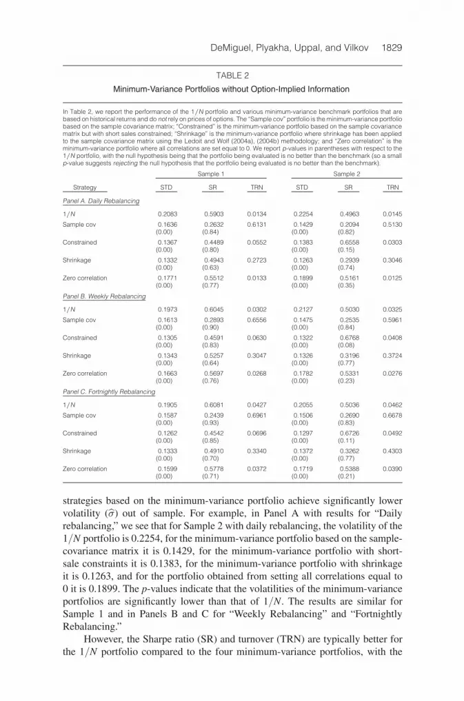
DeMiguel, Plyakha, Uppal, and Vilkov 1829
TABLE 2
Minimum-Variance Portfolios without Option-Implied Information
In Table 2, we report the performance of the 1/N portfolio and various minimum-variance benchmark portfolios that arebased on historical returns and do not rely on prices of options. The “Sample cov” portfolio is the minimum-variance portfoliobased on the sample covariance matrix; “Constrained” is the minimum-variance portfolio based on the sample covariancematrix but with short sales constrained; “Shrinkage” is the minimum-variance portfolio where shrinkage has been appliedto the sample covariance matrix using the Ledoit and Wolf (2004a), (2004b) methodology; and “Zero correlation” is theminimum-variance portfolio where all correlations are set equal to 0. We report p-values in parentheses with respect to the1/N portfolio, with the null hypothesis being that the portfolio being evaluated is no better than the benchmark (so a smallp-value suggests rejecting the null hypothesis that the portfolio being evaluated is no better than the benchmark).
Sample 1 Sample 2
Strategy STD SR TRN STD SR TRN
Panel A. Daily Rebalancing
1/N 0.2083 0.5903 0.0134 0.2254 0.4963 0.0145
Sample cov 0.1636 0.2632 0.6131 0.1429 0.2094 0.5130(0.00) (0.84) (0.00) (0.82)
Constrained 0.1367 0.4489 0.0552 0.1383 0.6558 0.0303(0.00) (0.80) (0.00) (0.15)
Shrinkage 0.1332 0.4943 0.2723 0.1263 0.2939 0.3046(0.00) (0.63) (0.00) (0.74)
Zero correlation 0.1771 0.5512 0.0133 0.1899 0.5161 0.0125(0.00) (0.77) (0.00) (0.35)
Panel B. Weekly Rebalancing
1/N 0.1973 0.6045 0.0302 0.2127 0.5030 0.0325
Sample cov 0.1613 0.2893 0.6556 0.1475 0.2535 0.5961(0.00) (0.90) (0.00) (0.84)
Constrained 0.1305 0.4591 0.0630 0.1322 0.6768 0.0408(0.00) (0.83) (0.00) (0.08)
Shrinkage 0.1343 0.5257 0.3047 0.1326 0.3196 0.3724(0.00) (0.64) (0.00) (0.77)
Zero correlation 0.1663 0.5697 0.0268 0.1782 0.5331 0.0276(0.00) (0.76) (0.00) (0.23)
Panel C. Fortnightly Rebalancing
1/N 0.1905 0.6081 0.0427 0.2055 0.5036 0.0462
Sample cov 0.1587 0.2439 0.6961 0.1506 0.2690 0.6678(0.00) (0.93) (0.00) (0.83)
Constrained 0.1262 0.4542 0.0696 0.1297 0.6726 0.0492(0.00) (0.85) (0.00) (0.11)
Shrinkage 0.1333 0.4910 0.3340 0.1372 0.3262 0.4303(0.00) (0.70) (0.00) (0.77)
Zero correlation 0.1599 0.5778 0.0372 0.1719 0.5388 0.0390(0.00) (0.71) (0.00) (0.21)
strategies based on the minimum-variance portfolio achieve significantly lowervolatility (σ) out of sample. For example, in Panel A with results for “Dailyrebalancing,” we see that for Sample 2 with daily rebalancing, the volatility of the1/N portfolio is 0.2254, for the minimum-variance portfolio based on the sample-covariance matrix it is 0.1429, for the minimum-variance portfolio with short-sale constraints it is 0.1383, for the minimum-variance portfolio with shrinkageit is 0.1263, and for the portfolio obtained from setting all correlations equal to0 it is 0.1899. The p-values indicate that the volatilities of the minimum-varianceportfolios are significantly lower than that of 1/N. The results are similar forSample 1 and in Panels B and C for “Weekly Rebalancing” and “FortnightlyRebalancing.”
However, the Sharpe ratio (SR) and turnover (TRN) are typically better forthe 1/N portfolio compared to the four minimum-variance portfolios, with the

1830 Journal of Financial and Quantitative Analysis
TABLE 3
Mean-Variance Portfolios without Option-Implied Information
In Table 3, we report the performance of the 1/N portfolio and various mean-variance portfolios that are based on historicalreturns and do not rely on prices of options. The “Sample cov” portfolio is the mean-variance portfolio based on the samplecovariance matrix; “Constrained” is the mean-variance portfolio based on the sample covariance matrix but with shortsales constrained; “Shrinkage” is the mean-variance portfolio where shrinkage has been applied to the sample covariancematrix using the Ledoit and Wolf (2004a), (2004b) methodology; “Zero correlation” is the mean-variance portfolio whereall correlations are set equal to 0; and “1/N + FFM” denotes the parametric benchmark portfolio, where we start with the“1/N” initial portfolio and adjust it optimally using the Fama-French and momentum characteristics. We report p-valuesin parentheses with respect to the 1/N portfolio, with the null hypothesis being that the portfolio being evaluated is nobetter than the benchmark (so a small p-value suggests rejecting the null hypothesis that the portfolio being evaluated isno better than the benchmark).
Sample 1 Sample 2
Strategy STD SR TRN STD SR TRN
Panel A. Daily Rebalancing
1/N 0.2083 0.5903 0.0134 0.2254 0.4963 0.0145
Sample cov 0.4204 –0.2277 3.7940 0.6481 –0.9411 4.6965(1.00) (0.99) (1.00) (1.00)
Constrained 0.1370 0.3553 0.0624 0.1377 0.6083 0.0321(0.00) (0.92) (0.00) (0.23)
Shrinkage 0.6747 –0.1630 3.9762 0.9947 –0.6261 6.9215(1.00) (0.99) (1.00) (1.00)
Zero correlation 0.5700 –0.0683 1.6410 0.3427 0.1929 0.3008(1.00) (0.98) (1.00) (0.91)
1/N + FFM 0.2079 0.6589 0.0515 0.2285 0.5453 0.0372(0.38) (0.06) (1.00) (0.14)
Panel B. Weekly Rebalancing
1/N 0.1973 0.6045 0.0302 0.2127 0.5030 0.0325
Sample cov 0.4404 –0.0664 4.0024 0.7402 –0.6171 7.0693(1.00) (0.99) (1.00) (1.00)
Constrained 0.1301 0.4018 0.0703 0.1301 0.6513 0.0426(0.00) (0.92) (0.00) (0.13)
Shrinkage 0.8527 –0.0660 5.3350 1.1251 –0.4198 26.4889(1.00) (0.99) (1.00) (1.00)
Zero correlation 0.6571 0.0195 2.5679 0.3980 0.2036 0.4230(1.00) (0.99) (1.00) (0.95)
1/N + FFM 0.1979 0.6725 0.0624 0.2156 0.5617 0.0508(0.66) (0.05) (0.94) (0.08)
Panel C. Fortnightly Rebalancing
1/N 0.1905 0.6081 0.0427 0.2055 0.5036 0.0462
Sample cov 0.4330 –0.0352 4.2037 0.8165 –0.5013 19.2794(1.00) (0.99) (1.00) (1.00)
Constrained 0.1250 0.4124 0.0769 0.1267 0.6582 0.0508(0.00) (0.90) (0.00) (0.13)
Shrinkage 0.8992 –0.0386 7.0368 1.1933 –0.3280 24.4343(1.00) (0.98) (1.00) (0.99)
Zero correlation 0.6616 0.1669 9.9765 0.4239 0.1704 0.3918(1.00) (0.96) (1.00) (0.96)
1/N + FFM 0.1903 0.6749 0.0719 0.2075 0.5657 0.0623(0.48) (0.06) (0.77) (0.08)
only exceptions being the Sharpe ratio for the constrained minimum-varianceportfolio, and for the minimum-variance portfolio obtained by setting allcorrelations equal to 0, in the case of Sample 2; but, for both cases the differ-ences are not statistically significant.19
19It might seem strange to evaluate the Sharpe ratio of minimum-variance portfolios, whoseobjective is to only minimize the volatility of the portfolio. This comparison is motivated by thestatement in Jagannathan and Ma ((2003), p. 1653) that “the global minimum variance portfolio has

DeMiguel, Plyakha, Uppal, and Vilkov 1831
Of the four minimum-variance portfolios that we consider, the short-sale-constrained portfolio and the portfolio obtained by setting all correlations equalto 0 have turnover that is comparable to that of the 1/N portfolio and substantiallylower than the turnover of the unconstrained “Sample cov” portfolio. This is truealso in the tables that follow, where we use option-implied information.
Table 3 reports the performance of four mean-variance portfolios, “Samplecov,” “Constrained,” “Shrinkage,” and “Zero correlation,” and the mean-varianceportfolio implemented using the parametric-portfolio methodology with the Famaand French characteristics along with momentum, which in the table is labeled“1/N + FFM.” The three mean-variance portfolios that do not have constraints onshort selling (“Sample cov,” “Shrinkage,” and “Zero correlation”) perform verypoorly along all metrics. The mean-variance strategy with short-sale constraintsachieves a lower volatility than the 1/N portfolio, but it has a lower Sharpe ra-tio and higher turnover than the 1/N portfolio and also the short-sale-constrainedminimum-variance portfolio considered in Table 2. The parametric portfolio usu-ally has the best Sharpe ratio compared to the 1/N portfolio and the other mean-variance portfolios (though the difference is not always statistically significant),with a turnover that is comparable to that of 1/N. The volatility of the parametricportfolio is higher than that of the short-sale-constrained mean-variance portfolioand the minimum-variance portfolios considered in Table 2, which is not sur-prising, given that this portfolio is not designed with the objective of minimizingvolatility.
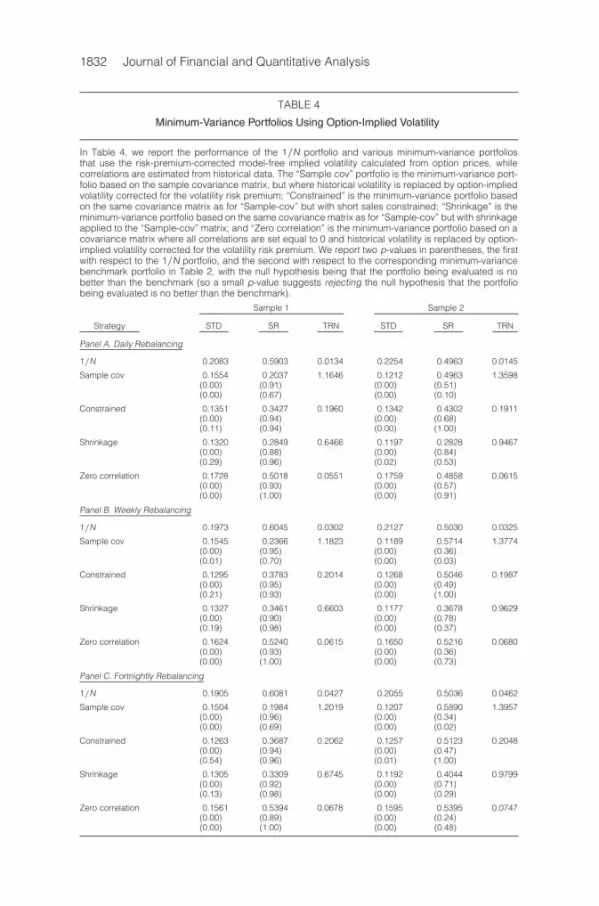
B. Performance of Portfolios Using Option-Implied Volatility
Motivated by the findings in Section V.A about the predictive power ofmodel-free implied volatilities after correction for the risk premium, RV, we usethem in diag(σ) to obtain the covariance matrix given in equation (9); that is,Σ=diag(RV) Ω diag(RV). Using this covariance matrix, and setting the expectedreturn on each asset equal to the grand mean across all stocks, we determine theminimum-variance portfolio in equation (8), along with the portfolios where shortsales are constrained, where shrinkage is applied to this covariance matrix, andwhere we impose the restriction that all correlations are equal to 0. In comput-ing these portfolios, we continue to use historical correlations (except for the lastportfolio, where correlations are set equal to 0).
The results for the minimum-variance portfolios based on risk-premium-corrected option-implied volatility are given in Table 4. In this table we reporttwo sets of p-values: the first with respect to the 1/N portfolio, and the secondwith respect to the corresponding benchmark portfolio in Table 2. For Sample 2,comparing the volatility (STD) of portfolio returns across the different portfo-lio strategies, we see that the “Shrinkage” portfolio always achieves the lowest
as large an out-of-sample Sharpe ratio as other efficient portfolios when past historical average returnsare used as proxies for expected returns.” DeMiguel, Garlappi, and Uppal (2009) also find that theminimum-variance portfolio performs surprisingly well in terms of Sharpe ratio when compared toother portfolios that rely on estimates of expected returns.
1832 Journal of Financial and Quantitative Analysis
TABLE 4
Minimum-Variance Portfolios Using Option-Implied Volatility
In Table 4, we report the performance of the 1/N portfolio and various minimum-variance portfoliosthat use the risk-premium-corrected model-free implied volatility calculated from option prices, whilecorrelations are estimated from historical data. The “Sample cov” portfolio is the minimum-variance port-folio based on the sample covariance matrix, but where historical volatility is replaced by option-impliedvolatility corrected for the volatility risk premium; “Constrained” is the minimum-variance portfolio basedon the same covariance matrix as for “Sample-cov” but with short sales constrained; “Shrinkage” is theminimum-variance portfolio based on the same covariance matrix as for “Sample-cov” but with shrinkageapplied to the “Sample-cov” matrix; and “Zero correlation” is the minimum-variance portfolio based on acovariance matrix where all correlations are set equal to 0 and historical volatility is replaced by option-implied volatility corrected for the volatility risk premium. We report two p-values in parentheses, the firstwith respect to the 1/N portfolio, and the second with respect to the corresponding minimum-variancebenchmark portfolio in Table 2, with the null hypothesis being that the portfolio being evaluated is nobetter than the benchmark (so a small p-value suggests rejecting the null hypothesis that the portfoliobeing evaluated is no better than the benchmark).
Sample 1 Sample 2
Strategy STD SR TRN STD SR TRN
Panel A. Daily Rebalancing
1/N 0.2083 0.5903 0.0134 0.2254 0.4963 0.0145
Sample cov 0.1554 0.2037 1.1646 0.1212 0.4963 1.3598(0.00) (0.91) (0.00) (0.51)(0.00) (0.67) (0.00) (0.10)
Constrained 0.1351 0.3427 0.1960 0.1342 0.4302 0.1911(0.00) (0.94) (0.00) (0.68)(0.11) (0.94) (0.00) (1.00)
Shrinkage 0.1320 0.2849 0.6466 0.1197 0.2828 0.9467(0.00) (0.88) (0.00) (0.84)(0.29) (0.96) (0.02) (0.53)
Zero correlation 0.1728 0.5018 0.0551 0.1759 0.4858 0.0615(0.00) (0.93) (0.00) (0.57)(0.00) (1.00) (0.00) (0.91)
Panel B. Weekly Rebalancing
1/N 0.1973 0.6045 0.0302 0.2127 0.5030 0.0325
Sample cov 0.1545 0.2366 1.1823 0.1189 0.5714 1.3774(0.00) (0.95) (0.00) (0.36)(0.01) (0.70) (0.00) (0.03)
Constrained 0.1295 0.3783 0.2014 0.1268 0.5046 0.1987(0.00) (0.95) (0.00) (0.49)(0.21) (0.93) (0.00) (1.00)
Shrinkage 0.1327 0.3461 0.6603 0.1177 0.3678 0.9629(0.00) (0.90) (0.00) (0.78)(0.19) (0.98) (0.00) (0.37)
Zero correlation 0.1624 0.5240 0.0615 0.1650 0.5216 0.0680(0.00) (0.93) (0.00) (0.36)(0.00) (1.00) (0.00) (0.73)
Panel C. Fortnightly Rebalancing
1/N 0.1905 0.6081 0.0427 0.2055 0.5036 0.0462
Sample cov 0.1504 0.1984 1.2019 0.1207 0.5890 1.3957(0.00) (0.96) (0.00) (0.34)(0.00) (0.69) (0.00) (0.02)
Constrained 0.1263 0.3687 0.2062 0.1257 0.5123 0.2048(0.00) (0.94) (0.00) (0.47)(0.54) (0.96) (0.01) (1.00)
Shrinkage 0.1305 0.3309 0.6745 0.1192 0.4044 0.9799(0.00) (0.92) (0.00) (0.71)(0.13) (0.98) (0.00) (0.29)
Zero correlation 0.1561 0.5394 0.0678 0.1595 0.5395 0.0747(0.00) (0.89) (0.00) (0.24)(0.00) (1.00) (0.00) (0.48)
DeMiguel, Plyakha, Uppal, and Vilkov 1833
volatility, and this is significantly lower than that of the 1/N portfolio and alsothe “Shrinkage” benchmark strategy in Table 2, which uses historical volatility;however, the “Shrinkage” strategy has the lowest Sharpe ratio of all the strategiesin Table 4, and also its turnover is quite high. For Sample 1, again the lowestvolatility for daily rebalancing is achieved by the “Shrinkage” strategy, but forweekly and fortnightly rebalancing, it is the constrained strategy that has the low-est volatility. For both samples and all three rebalancing frequencies, of the fourminimum-variance portfolios, it is the “Zero correlation” portfolio that achievesthe lowest turnover and the highest Sharpe ratio; for Sample 2, this Sharpe ratiois higher than even that of the 1/N portfolio.20
We conclude that volatility of stock returns estimated from risk-premium-corrected implied volatility is successful in achieving a significant reduction inportfolio volatility.21
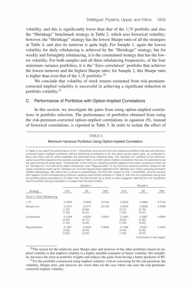
C. Performance of Portfolios with Option-Implied Correlations
In this section, we investigate the gains from using option-implied correla-tions in portfolio selection. The performance of portfolios obtained from usingthe risk-premium-corrected option-implied correlations in equation (9), insteadof historical correlations, is reported in Table 5. In order to isolate the effect of
TABLE 5
Minimum-Variance Portfolios Using Option-Implied Correlation
In Table 5, we report the performance of the 1/N portfolio and various minimum-variance portfolios that use risk-premium-corrected option-implied correlation without restricting correlations to be the same across asset pairs, as computed inBuss and Vilkov (2012), while volatilities are estimated from historical data. The “Sample cov” portfolio is the minimum-variance portfolio based on the sample covariance matrix, but with option-implied correlations that are not assumed to bethe same across all asset pairs; “Constrained” is the minimum-variance portfolio based on the same covariance matrix asfor “Sample-cov” but with short sales constrained; and “Regularization” is the minimum-variance portfolio based on thesame covariance matrix as for “Sample-cov” but with regularization applied to the “Sample-cov” matrix using the Zumbach(2009) methodology. We report two p-values in parentheses, the first with respect to the 1/N portfolio, and the secondwith respect to the corresponding minimum-variance benchmark portfolio in Table 2, with the null hypothesis being thatthe portfolio being evaluated is no better than the benchmark (so a small p-value suggests rejecting the null hypothesisthat the portfolio being evaluated is no better than the benchmark).
Sample 1 Sample 2
Strategy STD SR TRN STD SR TRN
Panel A. Daily Rebalancing
1/N 0.2083 0.5903 0.0134 0.2254 0.4963 0.0145
Sample cov 0.2374 0.2771 3.6129 0.2204 0.2838 4.4839(1.00) (0.84) (0.27) (0.76)(1.00) (0.47) (1.00) (0.37)
Constrained 0.1549 0.8235 0.0843 0.1803 0.5867 0.0895(0.00) (0.17) (0.00) (0.36)(1.00) (0.03) (1.00) (0.62)
Regularization 0.1367 0.6334 0.2659 0.1506 0.6321 0.4240(0.00) (0.43) (0.00) (0.26)(0.82) (0.25) (1.00) (0.07)
(continued on next page)
20The reason for the relatively poor Sharpe ratio and turnover of the other portfolios based on im-plied volatility is that implied volatility is a highly unstable estimator of future volatility; this instabil-ity increases the error in portfolio weights and reduces the gains from having a better predictor of RV.
21For the portfolio constructed using implied volatility without correcting for the risk premium, thevolatility, Sharpe ratio, and turnover are worse than for the case where one uses the risk-premium-corrected implied volatility.

1834 Journal of Financial and Quantitative Analysis
TABLE 5 (continued)
Minimum-Variance Portfolios Using Option-Implied Correlation
Sample 1 Sample 2
Strategy STD SR TRN STD SR TRN
Panel B. Weekly Rebalancing
1/N 0.1973 0.6045 0.0302 0.2127 0.5030 0.0325
Sample cov 0.2307 0.4974 3.6233 0.2034 0.3755 4.5216(1.00) (0.67) (0.16) (0.71)(1.00) (0.16) (1.00) (0.24)
Constrained 0.1416 0.7545 0.0879 0.1651 0.5673 0.0945(0.00) (0.22) (0.00) (0.36)(0.99) (0.03) (1.00) (0.71)
Regularization 0.1321 0.6429 0.2756 0.1454 0.6261 0.4381(0.00) (0.43) (0.00) (0.23)(0.28) (0.22) (0.99) (0.05)
Panel C. Fortnightly Rebalancing
1/N 0.1905 0.6081 0.0427 0.2055 0.5036 0.0462
Sample cov 0.2160 0.4381 3.6494 0.2117 0.2819 4.5829(0.98) (0.77) (0.71) (0.83)(1.00) (0.17) (1.00) (0.47)
Constrained 0.1347 0.7294 0.0909 0.1608 0.5446 0.0983(0.00) (0.27) (0.00) (0.40)(0.94) (0.05) (1.00) (0.73)
Regularization 0.1277 0.6214 0.2857 0.1431 0.6051 0.4522(0.00) (0.47) (0.00) (0.28)(0.12) (0.18) (0.83) (0.05)
using implied correlations, we use volatilities calculated from historical data whencomputing the portfolio weights.
We consider three minimum-variance portfolios in Table 5: The first is basedon the sample-covariance matrix with option-implied correlations; the second isthe same as the first, but with short sales constrained; and the third, which is la-beled “regularization,” replaces the “shrinkage” portfolio considered in the earliertables. We use the regularization approach of Zumbach (2009) because we are us-ing option-implied correlations and, hence, do not know the distribution of returnsfor the resulting covariance matrix, which means that we cannot use the shrinkageresults of Ledoit and Wolf (2004a), (2004b) that rely on particular distributionalassumptions.
We observe from Table 5 that using the risk-premium-corrected impliedcorrelations does not lead to much of an improvement in the out-of-sample per-formance of the minimum-variance portfolios.22 While the volatility of the port-folios with short-sale constraints and regularization is less than that of the 1/Nfor both Sample 1 and Sample 2, it exceeds that of the corresponding benchmarkportfolios studied in Table 2. The portfolios based on option-implied correlationsalso have higher turnover. The only positive result is that the Sharpe ratio of theconstrained portfolio is greater than that of the 1/N portfolio and also the corre-sponding benchmark portfolio in Table 2, though the improvement is not alwaysstatistically significant.
22The performance of portfolios based on implied correlations without the correction for the riskpremium is slightly worse.

DeMiguel, Plyakha, Uppal, and Vilkov 1835
Thus, we conclude that using the option-implied correlations does not leadto a significant improvement in portfolio performance. The reason for the poorperformance of portfolios based on implied correlations is that the covariancematrix based on these correlations is highly unstable over time. Consequently, theresulting portfolio weights are highly variable and perform poorly out of sample.
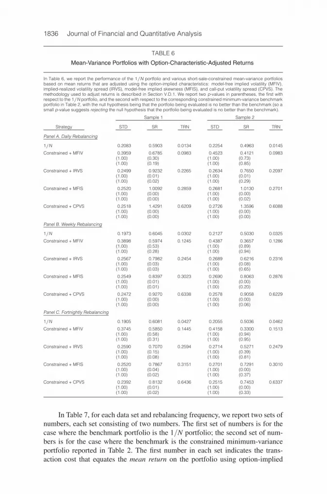
D. Performance of Portfolios with Returns Predicted Using Options
In this section, we examine the effect on portfolio performance of using fouroption-implied quantities that explain the cross section of stock returns: MFIV;volatility risk premium, measured as the spread between the currently observedBlack-Scholes (1973) option-implied volatility and realized (historical) volatility(IRVS); MFIS; and skewness, measured as the spread between the Black-Scholesimplied volatilities for calls and for puts (CPVS). There are two ways in whichwe use these quantities to improve the performance of portfolios. In the first,described in Section V.D.1, we rank all stocks based on each characteristic andadjust the returns of the top and bottom decile portfolios. In the second, describedin Section V.D.2, we use the parametric-portfolio methodology of Brandt et al.(2009).
1. Performance of a Mean-Variance Portfolio with Option Characteristics
The out-of-sample performance of the mean-variance portfolios that useoption-implied characteristics to adjust returns is reported in Table 6. There arefour portfolios, each with short-sale constraints, considered in this table corre-sponding to the following four option characteristics: MFIV, IRVS, MFIS, andCPVS. We compare performance of these portfolios to two sets of benchmarks:the 1/N portfolio and the constrained minimum-variance portfolio reported inTable 2, which does not rely on option prices.23
From Table 6, we see that other than MFIV, the portfolios whose returns areadjusted based on any of the other three characteristics have a significantly higherSharpe ratio than the 1/N portfolio and the benchmark portfolios in Table 3. Thedifference in Sharpe ratios is largest for daily rebalancing, and it declines as therebalancing frequency decreases. For example, for Sample 1, the Sharpe ratio forthe 1/N portfolio is 0.5903, while for the portfolio using IRVS it is 0.9232, for theportfolio using MFIS it is 1.0092, and for the portfolio using CPVS it is 1.4291.However, the improvement in the Sharpe ratio is accompanied by an increase inturnover.
To understand whether the mean-variance portfolios using option-impliedcharacteristics to forecast expected returns outperform the benchmark portfolioseven in the presence of transaction costs, we compute the equivalent transactioncost for each portfolio. Recall from Section IV.D that this is the transaction costlevel that equates the performance metric (mean return or Sharpe ratio) of a givenstrategy with that for the benchmark strategy.
23We use as a benchmark the short-sale-constrained minimum-variance portfolio rather than theconstrained mean-variance portfolios because the constrained minimum-variance portfolio has betterperformance in terms of all three metrics.
1836 Journal of Financial and Quantitative Analysis
TABLE 6
Mean-Variance Portfolios with Option-Characteristic-Adjusted Returns
In Table 6, we report the performance of the 1/N portfolio and various short-sale-constrained mean-variance portfoliosbased on mean returns that are adjusted using the option-implied characteristics: model-free implied volatility (MFIV),implied-realized volatility spread (IRVS), model-free implied skewness (MFIS), and call-put volatility spread (CPVS). Themethodology used to adjust returns is described in Section V.D.1. We report two p-values in parentheses, the first withrespect to the 1/N portfolio, and the second with respect to the corresponding constrained minimum-variance benchmarkportfolio in Table 2, with the null hypothesis being that the portfolio being evaluated is no better than the benchmark (so asmall p-value suggests rejecting the null hypothesis that the portfolio being evaluated is no better than the benchmark).
Sample 1 Sample 2
Strategy STD SR TRN STD SR TRN
Panel A. Daily Rebalancing
1/N 0.2083 0.5903 0.0134 0.2254 0.4963 0.0145
Constrained + MFIV 0.3959 0.6785 0.0983 0.4523 0.4121 0.0983(1.00) (0.30) (1.00) (0.73)(1.00) (0.19) (1.00) (0.85)
Constrained + IRVS 0.2499 0.9232 0.2265 0.2634 0.7650 0.2097(1.00) (0.01) (1.00) (0.01)(1.00) (0.02) (1.00) (0.29)
Constrained + MFIS 0.2520 1.0092 0.2859 0.2681 1.0130 0.2701(1.00) (0.00) (1.00) (0.00)(1.00) (0.00) (1.00) (0.02)
Constrained + CPVS 0.2518 1.4291 0.6209 0.2726 1.3596 0.6088(1.00) (0.00) (1.00) (0.00)(1.00) (0.00) (1.00) (0.00)
Panel B. Weekly Rebalancing
1/N 0.1973 0.6045 0.0302 0.2127 0.5030 0.0325
Constrained + MFIV 0.3898 0.5974 0.1245 0.4387 0.3657 0.1286(1.00) (0.53) (1.00) (0.89)(1.00) (0.28) (1.00) (0.94)
Constrained + IRVS 0.2567 0.7982 0.2454 0.2689 0.6216 0.2316(1.00) (0.03) (1.00) (0.08)(1.00) (0.03) (1.00) (0.65)
Constrained + MFIS 0.2549 0.8397 0.3023 0.2690 0.8063 0.2876(1.00) (0.01) (1.00) (0.00)(1.00) (0.01) (1.00) (0.20)
Constrained + CPVS 0.2472 0.9270 0.6338 0.2578 0.9058 0.6229(1.00) (0.00) (1.00) (0.00)(1.00) (0.00) (1.00) (0.06)
Panel C. Fortnightly Rebalancing
1/N 0.1905 0.6081 0.0427 0.2055 0.5036 0.0462
Constrained + MFIV 0.3745 0.5850 0.1445 0.4158 0.3300 0.1513(1.00) (0.58) (1.00) (0.94)(1.00) (0.31) (1.00) (0.95)
Constrained + IRVS 0.2590 0.7070 0.2594 0.2714 0.5271 0.2479(1.00) (0.15) (1.00) (0.39)(1.00) (0.08) (1.00) (0.81)
Constrained + MFIS 0.2520 0.7867 0.3151 0.2701 0.7291 0.3010(1.00) (0.04) (1.00) (0.00)(1.00) (0.02) (1.00) (0.37)
Constrained + CPVS 0.2392 0.8132 0.6436 0.2515 0.7453 0.6337(1.00) (0.01) (1.00) (0.00)(1.00) (0.02) (1.00) (0.33)
In Table 7, for each data set and rebalancing frequency, we report two sets ofnumbers, each set consisting of two numbers. The first set of numbers is for thecase where the benchmark portfolio is the 1/N portfolio; the second set of num-bers is for the case where the benchmark is the constrained minimum-varianceportfolio reported in Table 2. The first number in each set indicates the trans-action cost that equates the mean return on the portfolio using option-implied
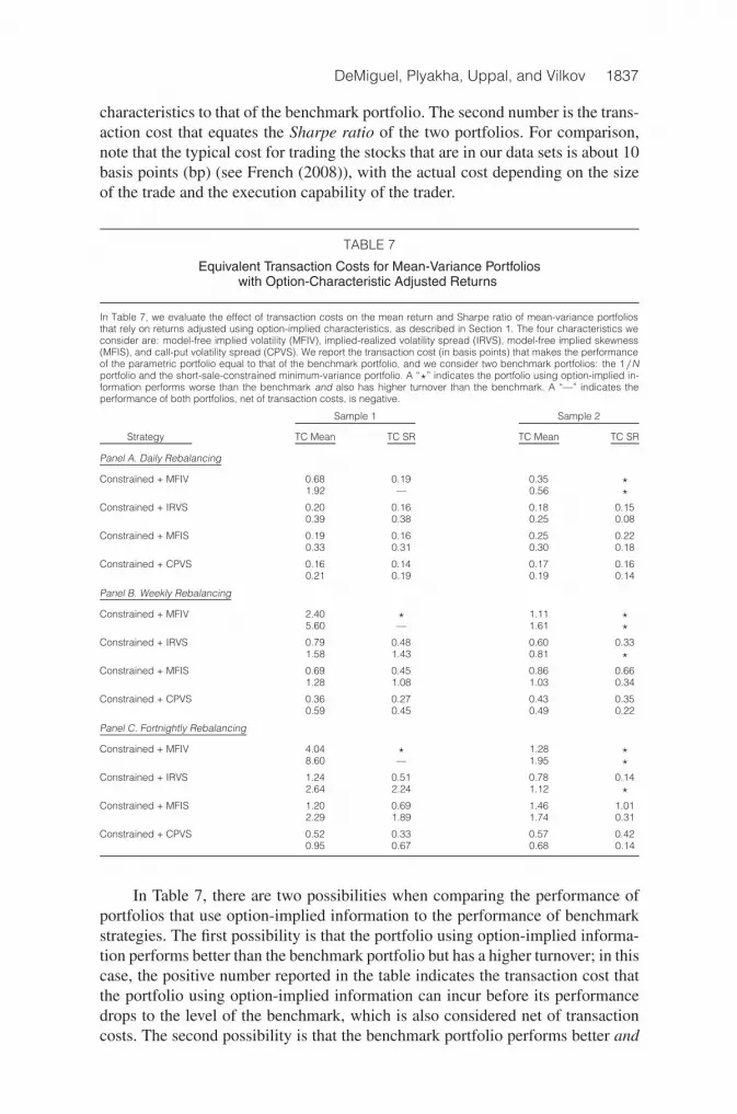
DeMiguel, Plyakha, Uppal, and Vilkov 1837
characteristics to that of the benchmark portfolio. The second number is the trans-action cost that equates the Sharpe ratio of the two portfolios. For comparison,note that the typical cost for trading the stocks that are in our data sets is about 10basis points (bp) (see French (2008)), with the actual cost depending on the sizeof the trade and the execution capability of the trader.
TABLE 7
Equivalent Transaction Costs for Mean-Variance Portfolioswith Option-Characteristic Adjusted Returns
In Table 7, we evaluate the effect of transaction costs on the mean return and Sharpe ratio of mean-variance portfoliosthat rely on returns adjusted using option-implied characteristics, as described in Section 1. The four characteristics weconsider are: model-free implied volatility (MFIV), implied-realized volatility spread (IRVS), model-free implied skewness(MFIS), and call-put volatility spread (CPVS). We report the transaction cost (in basis points) that makes the performanceof the parametric portfolio equal to that of the benchmark portfolio, and we consider two benchmark portfolios: the 1/Nportfolio and the short-sale-constrained minimum-variance portfolio. A “�” indicates the portfolio using option-implied in-formation performs worse than the benchmark and also has higher turnover than the benchmark. A “—” indicates theperformance of both portfolios, net of transaction costs, is negative.
Sample 1 Sample 2
Strategy TC Mean TC SR TC Mean TC SR
Panel A. Daily Rebalancing
Constrained + MFIV 0.68 0.19 0.35 �1.92 — 0.56 �
Constrained + IRVS 0.20 0.16 0.18 0.150.39 0.38 0.25 0.08
Constrained + MFIS 0.19 0.16 0.25 0.220.33 0.31 0.30 0.18
Constrained + CPVS 0.16 0.14 0.17 0.160.21 0.19 0.19 0.14
Panel B. Weekly Rebalancing
Constrained + MFIV 2.40 � 1.11 �5.60 — 1.61 �
Constrained + IRVS 0.79 0.48 0.60 0.331.58 1.43 0.81 �
Constrained + MFIS 0.69 0.45 0.86 0.661.28 1.08 1.03 0.34
Constrained + CPVS 0.36 0.27 0.43 0.350.59 0.45 0.49 0.22
Panel C. Fortnightly Rebalancing
Constrained + MFIV 4.04 � 1.28 �8.60 — 1.95 �
Constrained + IRVS 1.24 0.51 0.78 0.142.64 2.24 1.12 �
Constrained + MFIS 1.20 0.69 1.46 1.012.29 1.89 1.74 0.31
Constrained + CPVS 0.52 0.33 0.57 0.420.95 0.67 0.68 0.14
In Table 7, there are two possibilities when comparing the performance ofportfolios that use option-implied information to the performance of benchmarkstrategies. The first possibility is that the portfolio using option-implied informa-tion performs better than the benchmark portfolio but has a higher turnover; in thiscase, the positive number reported in the table indicates the transaction cost thatthe portfolio using option-implied information can incur before its performancedrops to the level of the benchmark, which is also considered net of transactioncosts. The second possibility is that the benchmark portfolio performs better and

1838 Journal of Financial and Quantitative Analysis
has better turnover; in this case, there is no positive level of transaction costs thatequates the performance of the two strategies, and we indicate this in the tablewith the symbol “�”. The third possibility is that the performance of both portfo-lios turns negative after adjustment for transaction costs; in the table, we use “—”to represent this case.
We observe from Panel A of Table 7 that for the case of daily rebalancing,the equivalent transaction cost for the Sharpe ratio ranges from 14 bp to 38 bp; forexample, in the case of Sample 2, the portfolio with returns adjusted using MFIShas a higher Sharpe ratio than the 1/N portfolio for transaction costs of up to22 bp. In Panels B and C, we see that as the rebalancing frequency decreases, andthe equivalent transaction cost increases; for example, in the case of Sample 2, theportfolio with returns adjusted using MFIS has a higher Sharpe ratio than the 1/Nportfolio for transaction costs of up to 66 bp for weekly rebalancing, and up to101 bp for fortnightly rebalancing.
We conclude from this analysis that information in MFIV, IRVS, MFIS, andCPVS can be used to improve the Sharpe ratio of mean-variance portfolios evenafter adjusting for the higher transaction cost as a consequence of higher turnoverin implementing the option-based strategy.
2. Performance of a Parametric Portfolio Based on Option Characteristics
Next, we examine the out-of-sample performance of the parametric port-folios that use option-implied characteristics. We consider two benchmark port-folios: the 1/N portfolio and the mean-variance parametric portfolio “1/N +FFM” that starts with the 1/N portfolio and uses the Fama-French and momentumcharacteristics to adjust the portfolio weights; we do not allow for short sales.Comparing the two benchmarks, we see that the 1/N portfolio has better turnoverand volatility, but the parametric portfolio has a better Sharpe ratio.
From Table 8, we see that when we use the option-implied characteristicsalone instead of the FFM, then the implied skewness measures (MFIS and CPVS)improve the risk-return tradeoff significantly compared to the two benchmarks.Moreover, the improvement over 1/N is significant for daily, weekly, and fort-nightly holding periods, while the improvement over the parametric portfolio issignificant only for daily rebalancing. For instance, in Panel A for Sample 1,the Sharpe ratio for the 1/N portfolio is 0.5903 and for the parametric portfoliowith FFM factors it is 0.6589, while for the parametric portfolio with IRVS it is0.6433, for the parametric portfolio with MFIS it is 0.7908, and for the parametricportfolio with CPVS it is 0.9390; the results are similar for Sample 2. However,these gains are accompanied by higher turnover. Note that as the rebalancing pe-riod increases, the improvement decreases, while turnover per rebalancing periodstays at about the same level. This implies that the total transaction cost paid overthe entire time period is decreasing.
We can also ask whether the option-implied characteristics improve perfor-mance if one is already using the traditional size, value, and momentum charac-teristics when selecting the parametric portfolio. This question is answered in thesecond part of each panel of Table 8, where we consider each option-implied char-acteristic in addition to the FFM characteristics considered in the benchmark port-folio. From the lower part of each panel, we see that MFIS and CPVS improve the

DeMiguel, Plyakha, Uppal, and Vilkov 1839
TABLE 8
Parametric Portfolios Using Option-Implied Information
In Table 8, we evaluate the performance of parametric portfolios that rely on option-implied characteristics about expectedreturns, using the methodology proposed in Brandt et al. (2009). In each panel, we first consider the effect of choosing aportfolio that is based on option-implied characteristic (individually and together), rather than the traditional FFM charac-teristics. The characteristics we consider are: model-free implied volatility (MFIV), implied-realized volatility spread (IRVS),model-free implied skewness (MFIS), and call-put volatility spread (CPVS). In the second part of each panel, we considerthe effect of considering these option-implied characteristics (individually and together) in addition to the FFM character-istics. We report two p-values in parentheses, the first with respect to the 1/N portfolio and the second with respect to the“1/N + FFM” portfolio, with the null hypothesis being that the portfolio being evaluated is no better than the benchmark(so a small p-value suggests rejecting the null hypothesis that the portfolio being evaluated is no better than the bench-mark).
Sample 1 Sample 2
Strategy STD SR TRN STD SR TRN
Panel A. Daily Rebalancing
1/N 0.2083 0.5903 0.0134 0.2254 0.4963 0.0145
1/N + FFM 0.2079 0.6589 0.0515 0.2285 0.5453 0.0372(0.38) (0.06) (1.00) (0.14)(0.50) (0.50) (0.50) (0.50)
1/N + MFIV 0.2142 0.6180 0.0780 0.2269 0.5063 0.0605(1.00) (0.33) (0.84) (0.44)(1.00) (0.75) (0.16) (0.74)
1/N + IRVS 0.2062 0.6433 0.0904 0.2246 0.5413 0.0855(0.00) (0.01) (0.19) (0.04)(0.09) (0.63) (0.00) (0.54)
1/N + MFIS 0.2143 0.7908 0.2033 0.2378 0.7075 0.1950(1.00) (0.00) (1.00) (0.00)(1.00) (0.01) (1.00) (0.00)
1/N + CPVS 0.2093 0.9390 0.2944 0.2300 0.8516 0.2935(0.98) (0.00) (1.00) (0.00)(0.87) (0.00) (0.92) (0.00)
1/N + ALL IMPLIED 0.2178 0.9269 0.3352 0.2346 0.8493 0.2844(1.00) (0.00) (1.00) (0.00)(1.00) (0.00) (1.00) (0.00)
1/N + FFM + MFIV 0.2140 0.6635 0.0891 0.2270 0.5714 0.0613(1.00) (0.12) (0.85) (0.09)(1.00) (0.47) (0.07) (0.23)
1/N + FFM + IRVS 0.2070 0.6645 0.0932 0.2257 0.5556 0.0607(0.08) (0.04) (0.60) (0.09)(0.02) (0.39) (0.00) (0.29)
1/N + FFM + MFIS 0.2091 0.7996 0.2011 0.2340 0.6649 0.1683(0.79) (0.00) (1.00) (0.00)(0.98) (0.00) (1.00) (0.00)
1/N + FFM + CPVS 0.2127 1.0174 0.3497 0.2333 0.8655 0.3047(1.00) (0.00) (1.00) (0.00)(1.00) (0.00) (1.00) (0.00)
1/N + FFM + ALL IMPLIED 0.2167 1.0184 0.3999 0.2351 0.8619 0.3164(1.00) (0.00) (1.00) (0.00)(1.00) (0.00) (1.00) (0.00)
Panel B. Weekly Rebalancing
1/N 0.1973 0.6045 0.0302 0.2127 0.5030 0.0325
1/N + FFM 0.1979 0.6725 0.0624 0.2156 0.5617 0.0508(0.66) (0.05) (0.94) (0.08)(0.50) (0.50) (0.50) (0.50)
1/N + MFIV 0.2046 0.6349 0.0880 0.2157 0.4965 0.0723(1.00) (0.30) (0.89) (0.55)(1.00) (0.76) (0.53) (0.89)
1/N + IRVS 0.1966 0.6270 0.0970 0.2144 0.5250 0.0938(0.23) (0.12) (0.94) (0.13)(0.25) (0.84) (0.30) (0.81)
1/N + MFIS 0.2045 0.6757 0.2064 0.2269 0.5884 0.1992(1.00) (0.00) (1.00) (0.00)(1.00) (0.47) (1.00) (0.26)
1/N + CPVS 0.1978 0.7034 0.2960 0.2167 0.6031 0.2956(0.91) (0.00) (1.00) (0.00)(0.46) (0.23) (0.75) (0.13)
(continued on next page)

1840 Journal of Financial and Quantitative Analysis
TABLE 8 (continued)
Parametric Portfolios Using Option-Implied Information
Sample 1 Sample 2
Strategy STD SR TRN STD SR TRN
Panel B. Weekly Rebalancing (continued)
1/N + ALL IMPLIED 0.2074 0.6915 0.3372 0.2215 0.6097 0.2869(1.00) (0.01) (1.00) (0.00)(1.00) (0.33) (1.00) (0.11)
1/N + FFM + MFIV 0.2042 0.6697 0.0973 0.2149 0.5732 0.0724(1.00) (0.11) (0.80) (0.07)(1.00) (0.52) (0.34) (0.35)
1/N + FFM + IRVS 0.1963 0.6700 0.1006 0.2141 0.5505 0.0712(0.31) (0.04) (0.79) (0.11)(0.01) (0.56) (0.02) (0.78)
1/N + FFM + MFIS 0.1990 0.7075 0.2044 0.2237 0.5760 0.1729(0.88) (0.00) (1.00) (0.01)(0.90) (0.06) (1.00) (0.31)
1/N + FFM + CPVS 0.2021 0.7538 0.3511 0.2209 0.6168 0.3068(1.00) (0.00) (1.00) (0.00)(1.00) (0.01) (1.00) (0.04)
1/N + FFM + ALL IMPLIED 0.2075 0.7600 0.4014 0.2235 0.6284 0.3185(1.00) (0.00) (1.00) (0.00)(1.00) (0.01) (1.00) (0.01)
Panel C. Fortnightly Rebalancing
1/N 0.1905 0.6081 0.0427 0.2055 0.5036 0.0462
1/N + FFM 0.1903 0.6749 0.0719 0.2075 0.5657 0.0623(0.48) (0.06) (0.77) (0.08)(0.50) (0.50) (0.50) (0.50)
1/N + MFIV 0.1979 0.6441 0.0972 0.2084 0.5023 0.0830(0.99) (0.29) (0.82) (0.53)(1.00) (0.71) (0.61) (0.88)
1/N + IRVS 0.1913 0.6226 0.1036 0.2085 0.5114 0.1020(0.74) (0.20) (0.98) (0.33)(0.64) (0.87) (0.66) (0.90)
1/N + MFIS 0.1986 0.6631 0.2103 0.2205 0.5585 0.2041(1.00) (0.00) (1.00) (0.00)(1.00) (0.59) (1.00) (0.58)
1/N + CPVS 0.1911 0.6627 0.2984 0.2094 0.5559 0.2985(0.92) (0.00) (1.00) (0.00)(0.61) (0.60) (0.79) (0.59)
1/N + ALL IMPLIED 0.2008 0.6662 0.3398 0.2137 0.5678 0.2901(1.00) (0.05) (1.00) (0.00)(1.00) (0.58) (0.99) (0.49)
1/N + FFM + MFIV 0.1973 0.6712 0.1051 0.2078 0.5665 0.0825(0.98) (0.15) (0.76) (0.11)(1.00) (0.55) (0.57) (0.49)
1/N + FFM + IRVS 0.1897 0.6681 0.1076 0.2068 0.5480 0.0808(0.36) (0.07) (0.70) (0.13)(0.22) (0.67) (0.23) (0.91)
1/N + FFM + MFIS 0.1926 0.7030 0.2084 0.2163 0.5484 0.1782(0.86) (0.00) (1.00) (0.07)(0.99) (0.12) (1.00) (0.72)
1/N + FFM + CPVS 0.1957 0.7165 0.3533 0.2146 0.5731 0.3097(1.00) (0.00) (1.00) (0.00)(1.00) (0.11) (1.00) (0.41)
1/N + FFM + ALL IMPLIED 0.2009 0.7286 0.4034 0.2166 0.5865 0.3212(1.00) (0.00) (1.00) (0.00)(1.00) (0.06) (1.00) (0.24)

DeMiguel, Plyakha, Uppal, and Vilkov 1841
Sharpe ratio beyond the gains obtained from using only the FFM characteristics.This improvement in Sharpe ratio for daily rebalancing is statistically significantfor both Samples 1 and 2 when using MFIS and CPVS; for weekly rebalancing,it is statistically significant for CPVS for both samples, and for MFIS only forSample 1; and it is not statistically significant for fortnightly rebalancing. Finally,looking at the last row of each panel, where we add all four option-implied charac-teristics to the portfolio that already considers the FFM characteristics, we observethat the Sharpe ratio increases substantially, and this improvement is statisticallysignificant for daily and weekly rebalancing for both samples; for fortnightlyrebalancing it is significant for Sample 1.
To understand if the parametric portfolios using option-implied character-istics outperform the benchmark portfolios even in the presence of transactioncosts, just as before, we compute the equivalent transaction cost for each port-folio. In Table 9, for each data set and rebalancing frequency, we report two setsof numbers, each set having two numbers. The first set of numbers is for the casewhere the benchmark portfolio is the 1/N portfolio; the second set of numbersis for the case where the benchmark is the parametric portfolio with the FFMcharacteristics.
TABLE 9
Equivalent Transaction Costs for Parametric Portfolios Using Option-Implied Information
In Table 9, we evaluate the effect of transaction costs on the mean return and Sharpe ratio of parametric portfolios thatrely on option-implied characteristics, using the methodology proposed in Brandt et al. (2009). The four characteristicswe consider (individually and together) are: model-free implied volatility (MFIV), implied-realized volatility spread (IRVS),model-free implied skewness (MFIS), and call-put volatility spread (CPVS). In the second part of each panel, we considerthe effect of considering these option-implied characteristics (individually and together) in addition to the FFM character-istics. We report the transaction cost (in basis points) that makes the performance of the parametric portfolio equal to thatof the benchmark portfolio, and we consider two benchmark portfolios: the 1/N portfolio and the “1/N + FFM” parametricportfolio. A “�” indicates the portfolio using option-implied information performs worse than the benchmark and also hashigher turnover than the benchmark.
Sample 1 Sample 2
Strategy TC Mean TC SR TC Mean TC SR
Panel A. Daily Rebalancing
1/N + MFIV 0.06 0.04 0.03 0.02� � � �
1/N + IRVS 0.05 0.06 0.05 0.06� � � �
1/N + MFIS 0.10 0.09 0.12 0.110.09 0.07 0.11 0.10
1/N + CPVS 0.10 0.10 0.12 0.120.10 0.10 0.11 0.11
1/N + ALL IMPLIED 0.10 0.09 0.13 0.120.09 0.08 0.12 0.12
1/N + FFM + MFIV 0.10 0.08 0.15 0.150.05 0.01 0.08 0.10
1/N + FFM + IRVS 0.07 0.08 0.12 0.120.00 0.01 0.01 0.04
1/N + FFM + MFIS 0.09 0.09 0.11 0.100.08 0.08 0.09 0.09
1/N + FFM + CPVS 0.11 0.11 0.12 0.120.11 0.10 0.12 0.11
1/N + FFM + ALL IMPLIED 0.10 0.10 0.12 0.110.10 0.09 0.11 0.11
(continued on next page)

1842 Journal of Financial and Quantitative Analysis
TABLE 9 (continued)
Equivalent Transaction Costs for Parametric Portfolios Using Option-Implied Information
Sample 1 Sample 2
Strategy TC Mean TC SR TC Mean TC SR
Panel B. Weekly Rebalancing
1/N + MFIV 0.37 0.22 0.01 �� � � �
1/N + IRVS 0.12 0.13 0.18 0.15� � � �
1/N + MFIS 0.21 0.17 0.32 0.230.07 0.01 0.17 0.08
1/N + CPVS 0.15 0.15 0.18 0.160.05 0.05 0.08 0.07
1/N + ALL IMPLIED 0.16 0.12 0.22 0.190.07 0.03 0.12 0.09
1/N + FFM + MFIV 0.52 0.40 0.81 0.760.21 � 0.19 0.23
1/N + FFM + IRVS 0.35 0.36 0.56 0.53� � � �
1/N + FFM + MFIS 0.25 0.23 0.31 0.230.11 0.10 0.13 0.05
1/N + FFM + CPVS 0.21 0.19 0.21 0.180.13 0.11 0.12 0.10
1/N + FFM + ALL IMPLIED 0.21 0.17 0.23 0.200.14 0.11 0.14 0.11
Panel C. Fortnightly Rebalancing
1/N + MFIV 0.85 0.53 0.13 �� � � �
1/N + IRVS 0.21 0.18 0.22 0.12� � � �
1/N + MFIS 0.38 0.26 0.50 0.310.09 � 0.16 �
1/N + CPVS 0.17 0.16 0.20 0.17� � � �
1/N + ALL IMPLIED 0.24 0.16 0.29 0.230.08 � 0.07 0.01
1/N + FFM + MFIV 1.06 0.82 1.56 1.460.48 � 0.07 0.03
1/N + FFM + IRVS 0.67 0.70 1.14 1.07� � � �
1/N + FFM + MFIS 0.47 0.44 0.46 0.300.20 0.16 0.04 �
1/N + FFM + CPVS 0.31 0.27 0.29 0.230.17 0.12 0.09 0.03
1/N + FFM + ALL IMPLIED 0.34 0.27 0.34 0.260.22 0.13 0.15 0.07
We observe from Panel A of Table 9 that for the case of daily rebalancing,the benefits of using option-implied information would be eliminated if one had topay a transaction cost of more than 11 bp. This is because of the relatively higherturnover of the strategies using option-implied information. However, when werebalance less frequently, the benefits of using option-implied information survivehigher transaction costs. For example, the results in Panel C for fortnightly rebal-ancing indicate that MFIS improves performance relative to the 1/N strategy evenwhen we pay transaction costs of about 30 bp. However, option-implied charac-teristics improve performance relative to the benchmark parametric portfolio for

DeMiguel, Plyakha, Uppal, and Vilkov 1843
transaction costs of up to 10 bp. Using all of the implied characteristics is bene-ficial in the presence of transaction costs of about 20 bp with respect to the 1/Nbenchmark, and about 10 bp for the parametric-portfolio benchmark.
In summary, Table 9 suggests that in the presence of transaction costs, MFISand CPVS are useful characteristics for choosing portfolios, while the value ofusing other characteristics is smaller, and their contribution is not robust across thetwo samples. Overall, the empirical evidence suggests that using option-impliedskewness can lead to an improvement in the out-of-sample portfolio Sharpe ratio,even after adjusting for the higher transaction costs incurred by these strategies.
VI. Conclusion
Mean-variance portfolio weights depend on estimates of volatilities, correla-tions, and expected returns of stocks. In this paper, we have studied how informa-tion implied in prices of stock options can be used to improve estimates of thesethree moments in order to improve the out-of-sample performance of portfolioswith a large number of stocks. Performance is measured in terms of portfoliovolatility, Sharpe ratio, and turnover. The benchmark portfolios are the 1/N port-folio; four types of minimum-variance portfolios and four types of mean-varianceportfolios based on historical returns; and the parametric portfolios of Brandt et al.(2009), based on historical returns and size, value, and momentum characteristics.
We find that using option-implied volatilities can lead to a significant im-provement in portfolio volatility; however, option-implied correlations are lessuseful in reducing portfolio volatility. We also find that forming portfolios usingexpected returns that exploit information in option-implied model-free skewnessand implied volatility achieve a higher Sharpe ratio than portfolios that ignoreoption-implied information; this improvement in performance is present even af-ter adjusting for transaction costs. Based on our empirical analysis, we concludethat prices of stock options contain information that can be useful for improvingthe out-of-sample performance of portfolios.
ReferencesAıt-Sahalia, Y., and M. W. Brandt. “Consumption and Portfolio Choice with Option-Implied State
Prices.” NBER Working Paper (2008).Andersen, T. G.; T. Bollerslev; and F. X. Diebold. “Parametric and Nonparametric Measurement
of Volatility.” In Handbook of Financial Econometrics, Y. Aıt-Sahalia, and L. P. Hansen, eds.Amsterdam: North Holland (2009).
Ang, A.; T. G. Bali; and N. Cakici. “The Joint Cross Section of Stocks and Options.” Working Paper,Fordham University (2010).
Bakshi, G. S.; N. Kapadia; and D. B. Madan. “Stock Return Characteristics, Skew Laws, andthe Differential Pricing of Individual Equity Options.” Review of Financial Studies, 16 (2003),101–143.
Bali, T. G., and A. Hovakimian. “Volatility Spreads and Expected Stock Returns.” ManagementScience, 55 (2009), 1797–1812.
Black, F., and M. S. Scholes. “The Pricing of Options and Corporate Liabilities.” Journal of PoliticalEconomy, 81 (1973), 637–659.
Bollerslev, T.; M. Gibson; and H. Zhou. “Dynamic Estimation of Volatility Risk Premia and InvestorRisk Aversion from Option-Implied and Realized Volatilities.” Finance and Economics DiscussionSeries, 2004-56, Board of Governors of the Federal Reserve System, Washington, DC (2004).
Bollerslev, T.; G. Tauchen; and H. Zhou. “Expected Stock Returns and Variance Risk Premia.” Reviewof Financial Studies, 22 (2009), 4463–4492.
1844 Journal of Financial and Quantitative Analysis
Boyer, B. H.; T. Mitton; and K. Vorkink. “Expected Idiosyncratic Skewness.” Review of FinancialStudies, 23 (2010), 169–202.
Brandt, M. W.; P. Santa-Clara; and R. Valkanov. “Parametric Portfolio Policies: Exploiting Character-istics in the Cross Section of Equity Returns.” Review of Financial Studies, 22 (2009), 3411–3447.
Buss, A., and G. Vilkov. “Measuring Equity Risk with Option-Implied Correlations.” Review ofFinancial Studies, 25 (2012), 3113–3140.
Carr, P., and L. Wu. “Variance Risk Premiums.” Review of Financial Studies, 22 (2009), 1311–1341.Chan, L. K. C.; J. Karceski; and J. Lakonishok. “On Portfolio Optimization: Forecasting Covariances
and Choosing the Risk Model.” Review of Financial Studies, 12 (1999), 937–974.Corsi, F. “A Simple Approximate Long-Memory Model of Realized Volatility.” Journal of Financial
Econometrics, 7 (2009), 174–196.Cox, J. C., and C.-F. Huang. “Optimal Consumption and Portfolio Policies When Asset Prices Follow
a Diffusion Process.” Journal of Economic Theory, 49 (1989), 33–83.Cremers, M., and D. Weinbaum. “Deviations from Put-Call Parity and Stock Return Predictability.”
Journal of Financial and Quantitative Analysis, 45 (2010), 335–367.DeMiguel, V.; L. Garlappi; F. Nogales; and R. Uppal. “A Generalized Approach to Portfolio
Optimization: Improving Performance by Constraining Portfolio Norms.” Management Science,55 (2009), 798–812.
DeMiguel, V.; L. Garlappi; and R. Uppal. “Optimal versus Naive Diversification: How Inefficient Isthe 1/N Portfolio Strategy?” Review of Financial Studies, 22 (2009), 1915–1953.
Driessen, J.; P. Maenhout; and G. Vilkov. “The Price of Correlation Risk: Evidence from EquityOptions.” Journal of Finance, 64 (2009), 1375–1404.
Efron, B., and R. Tibshirani. An Introduction to the Bootstrap. Boca Raton, FL: Chapman and Hall(1993).
Elton, E. J.; M. J. Gruber; and J. Spitzer. “Improved Estimates of Correlation Coefficients and TheirImpact on Optimum Portfolios.” European Financial Management, 12 (2006), 303–318.
Fama, E. F., and K. R. French. “The Cross-Section of Expected Stock Returns.” Journal of Finance,47 (1992), 427–465.
French, K. R. “Presidential Address: The Cost of Active Investing.” Journal of Finance, 63 (2008),1537–1573.
Goyal, A., and A. Saretto. “Cross-Section of Option Returns and Volatility.” Journal of FinancialEconomics, 94 (2009), 310–326.
Grundy, B. D., and S. Martin. “Understanding the Nature of the Risks and the Source of the Rewardsto Momentum Investing.” Review of Financial Studies, 14 (2001), 29–78.
Guidolin, M., and A. Timmermann. “International Asset Allocation under Regime Switching, Skewand Kurtosis Preferences.” Review of Financial Studies, 21 (2008), 889–935.
Harvey, C. R., and A. Siddique. “Conditional Skewness in Asset Pricing Tests.” Journal of Finance,55 (2000), 1263–1295.
Jacobs, H.; S. Muller; and M. Weber. “How Should Private Investors Diversify? An Empirical Evalu-ation of Alternative Asset Allocation Policies to Construct a ‘World Market Portfolio’.” WorkingPaper, University of Mannheim (2010).
Jagannathan, R., and T. Ma. “Risk Reduction in Large Portfolios: Why Imposing the Wrong Con-straints Helps.” Journal of Finance, 58 (2003), 1651–1684.
Jegadeesh, N., and S. Titman. “Returns to Buying Winners and Selling Losers: Implications for StockMarket Efficiency.” Journal of Finance, 48 (1993), 65–91.
Jobson, J. D.; R. Korkie; and V. Ratti. “Improved Estimation for Markowitz Portfolios Using James-Stein Type Estimators.” Proceedings of the American Statistical Association, 41 (1979), 279–284.
Jorion, P. “Bayes-Stein Estimation for Portfolio Analysis.” Journal of Financial and QuantitativeAnalysis, 21 (1986), 279–292.
Kostakis, A.; N. Panigirtzoglou; and G. Skiadopoulos. “Market Timing with Option-Implied Distri-butions: A Forward-Looking Approach.” Management Science, 57 (2011),1231–1249.
Kraus, A., and R. H. Litzenberger. “Skewness Preference and the Valuation of Risk Assets.” Journalof Finance, 31 (1976), 1085–1100.
Ledoit, O., and M. Wolf. “Honey, I Shrunk the Sample Covariance Matrix.” Journal of PortfolioManagement, 30 (2004a), 110–119.
Ledoit, O., and M. Wolf. “A Well-Conditioned Estimator for Large-Dimensional Covariance Matri-ces.” Journal of Multivariate Analysis, 88 (2004b), 365–411.
Ledoit, O., and M. Wolf. “Robust Performance Hypothesis Testing with the Sharpe Ratio.” Journalof Empirical Finance, 15 (2008), 850–859.
Merton, R. C. “Optimum Consumption and Portfolio Rules in a Continuous-Time Model.” Journalof Economic Theory, 3 (1971), 373–413.
Merton, R. C. “Theory of Rational Option Pricing.” Bell Journal of Economics and ManagementScience, 4 (1973), 141–183.

DeMiguel, Plyakha, Uppal, and Vilkov 1845
Newey, W. K., and K. D. West. “A Simple, Positive-Semidefinite, Heteroskedasticity and Autocorre-lation Consistent Covariance Matrix.” Econometrica, 55 (1987), 703–708.
Pastor, L. “Portfolio Selection and Asset Pricing Models.” Journal of Finance, 55 (2000), 179–223.Politis, D., and J. Romano. “The Stationary Bootstrap.” Journal of the American Statistical Associa-
tion, 89 (1994), 1303–1313.Poon, S.-H., and C. W. J. Granger. “Practical Issues in Forecasting Volatility.” Financial Analysts
Journal, 61 (2005), 45–56.Rehman, Z., and G. Vilkov. “Risk-Neutral Skewness: Return Predictability and Its Sources.” Working
Paper, Goethe University Frankfurt (2009).Rubinstein, M. E. “The Fundamental Theorem of Parameter-Preference Security Valuation.” Journal
of Financial and Quantitative Analysis, 8 (1973), 61–69.Vanden, J. M. “Information Quality and Options.” Review of Financial Studies, 21 (2008), 2635–2676.Xing, Y.; X. Zhang; and R. Zhao. “What Does Individual Option Volatility Smirk Tell Us About
Future Equity Returns?” Journal of Financial and Quantitative Analysis, 45 (2010), 641–662.Zumbach, G. “Inference on Multivariate ARCH Processes with Large Sizes.” Available at
http://dx.doi.org/10.2139/ssrn.1346416 (2009).