improving ensemble streamflow prediction using interdecadal
TRANSCRIPT

UNLV Theses, Dissertations, Professional Papers, and Capstones
12-2010
Improving ensemble streamflow prediction using interdecadal/Improving ensemble streamflow prediction using interdecadal/
interannual climate variability interannual climate variability
Kenneth W. Lamb University of Nevada, Las Vegas
Follow this and additional works at: https://digitalscholarship.unlv.edu/thesesdissertations
Part of the Civil and Environmental Engineering Commons, Climate Commons, Environmental
Monitoring Commons, and the Water Resource Management Commons
Repository Citation Repository Citation Lamb, Kenneth W., "Improving ensemble streamflow prediction using interdecadal/interannual climate variability" (2010). UNLV Theses, Dissertations, Professional Papers, and Capstones. 718. http://dx.doi.org/10.34917/1945917
This Dissertation is protected by copyright and/or related rights. It has been brought to you by Digital Scholarship@UNLV with permission from the rights-holder(s). You are free to use this Dissertation in any way that is permitted by the copyright and related rights legislation that applies to your use. For other uses you need to obtain permission from the rights-holder(s) directly, unless additional rights are indicated by a Creative Commons license in the record and/or on the work itself. This Dissertation has been accepted for inclusion in UNLV Theses, Dissertations, Professional Papers, and Capstones by an authorized administrator of Digital Scholarship@UNLV. For more information, please contact [email protected].
ii
IMPROVING ENSEMBLE STREAMFLOW PREDICTION USING
INTERDECADAL/INTERANNUAL CLIMATE VARIABILITY
by
Kenneth W. Lamb
Bachelor of Science, Civil Engineering University of Nevada, Las Vegas
2003
Masters of Civil Engineering Norwich University
2007
A dissertation submitted in partial fulfillments of the requirements for the
Doctor of Philosophy in Engineering
Department of Civil and Environmental Engineering
Howard R. Hughes College of Engineering
Graduate College
University of Nevada, Las Vegas
December 2010

iii
Copyright by Kenneth W. Lamb 2011 All Rights Reserved

ii
THE GRADUATE COLLEGE We recommend the dissertation prepared under our supervision by
Kenneth W. Lamb
entitled
Improving Ensemble Streamflow Prediction Using Interdecadal/
Interannual Climate Variability
be accepted in partial fulfillment of the requirements for the degree of Doctor of Philosophy in Engineering Civil and Environmental Engineering Thomas C. Piechota, Committee Chair Jacimaria Batista, Committee Member Sajjad Ahmad, Committee Member Ashok K. Singh, Committee Member Susanna Priest, Graduate Faculty Representative Ronald Smith, Ph. D., Vice President for Research and Graduate Studies and Dean of the Graduate College December 2010
iii
ABSTRACT
Improving Ensemble Streamflow Prediction Using
Interdecadal/Interannual Climate Variability
by
Kenneth W. Lamb
Thomas C. Piechota, Examination Committee Chair Professor of Civil Engineering
University of Nevada, Las Vegas
The National Weather Service’s (NWS) river forecast centers provide long-term
water resource forecasts for the main river basins in the U.S. The NWS creates seasonal
streamflow forecasts using an ensemble prediction model called the Extended
Streamflow Prediction (ESP) software. ESP creates runoff volume forecasts by taking
the current observed soil moisture and snowpack conditions in the basin and applying
them to historical temperature and precipitation scenarios. The ESP treats every historic
input year as a likely scenario of future basin conditions. Therefore improving the
knowledge about how long-term climate cycles impact streamflow can extend the
forecast lead time and improve the quality of long-lead forecasts.
First, a study of the existing climate indices is carried out in Chapter 3 to establish
which index shows a significant long-lead connection to the Colorado River Basin
(CRB). Using Singular Value Decomposition (SVD) this step identifies a 1-year lagged
relationship between the Pacific Ocean sea surface temperatures (SST) and CRB
streamflow. A new SST region is identified in this analysis (named the Hondo region)
and compared to the other established climate indices (e.g. SOI, PDO, NAO, AMO). The
tests demonstrate Hondo performs better at longer lead times than the existing climate
indices.

iv
Second, Chapter 4 identifies the climate cycles impacting the CRB streamflow.
The SVD analysis performed in Chapter 3 is extended to include the simultaneous (or 0-
year lag) as well as the 2nd and 3rd year lag times. Because SST’s and streamflow are
basically independent data, this chapter explains the physical connection between them
by analyzing the relationship between the ocean, atmosphere and CRB streamflow. This
analysis, as well as recent research into the Pacific Quasi-Decadal Oscillation (PQDO),
demonstrates that the CRB streamflow is dominated by a hierarchy of climate drivers.
The Hondo is the secondary level which exists between the extreme impacts of the ENSO
signal and the longer cyclical patters observed in the PQDO. The current research shows
that the QDO cycle leads precipitation by three years, and the Hondo leads the CRB by
one to two years.
Finally, the information from Chapter 4 reveals that the Hondo region can be used
as a basis for weighing the ESP output. This is done because water resource managers
create multi-year water plans that are utilized to project power generation supplies and
water system improvements. In Chapter 5 several methods of weighing the ESP output
based on the Hondo region are presented. Each method is assessed using parametric and
non-parametric forecast skill metrics. The overall goal of this chapter is to identify a
weighting technique, lag time, and season interval which show a marked improvement
over simply using the 30-year mean as a streamflow predictor. From this analysis the
forecast skill score is optimized when using the January – March average SST values as a
basis for forecasting the streamflow for the following water year.
v
TABLE OF CONTENTS
ABSTRACT ............................................................................................................... iii LIST OF FIGURES ..................................................................................................... viii CHAPTER 1 INTRODUCTION .................................................................................... 1
1.1 Research Problem ............................................................................................. 1
1.2 Long Lead Ensemble Streamflow Forecasting ................................................... 2
1.3 Water Resource Planning Forecasts in the Colorado River Basin....................... 3
1.3.1 CRB Forecasts and the 24-Month Study ............................................ 5
1.4 Existing CRB-Climate Teleconnections ............................................................ 6
1.5 Research Questions ........................................................................................... 8
1.6 Research Tasks – Question 1 ............................................................................. 9
1.6.1 Establishing a Long Lead Climate-Streamflow Teleconnection ......... 9
1.6.2 Defining the SST-Streamflow Teleconnection ................................. 10
1.6.3 Inter-comparison of Climate Indices ................................................ 12
1.6.4 Testing Forecast Potential ............................................................... 13
1.7 Research Tasks – Question 2 ........................................................................... 14
1.7.1 Extended SVD and Correlation Analysis ......................................... 14
1.7.2 Comparison With Current Research ................................................ 15
1.8 Research Tasks – Question 3 ........................................................................... 17
1.8.1 Weight Kernel Selection .................................................................. 17
1.8.2 Cross-Validation Forecast Skill ....................................................... 20
CHAPTER 2 LITERATURE REVIEW ....................................................................... 22
2.1 Introduction .................................................................................................... 22
2.2 Streamflow Forecasting ................................................................................... 22
2.3 Pacific Ocean Climate Indices ......................................................................... 24
2.3.2 Pacific Decadal Oscillation.............................................................. 27
2.4 Atlantic Ocean Climate Indices ....................................................................... 29
2.4.1 Northern Atlantic Oscillation........................................................... 29
2.5 Global Gridded Climate Data .......................................................................... 34
2.5.1 Sea Surface Temperature Data......................................................... 34
2.5.2 Geopotential Height ........................................................................ 38
2.5.3 Zonal Wind Field ............................................................................ 38
2.6 Colorado River Basin Streamflow/Forecast Data ............................................. 40
2.7 Summary of Data ............................................................................................ 42
CHAPTER 3 A BASIS FOR IMPROVING STREAMFLOW FORECASTING OF THE
COLORADO RIVER BASIN ................................................................ 44
3.1 Introduction .................................................................................................... 44
3.2 Data 47
3.2.1 Naturalized Streamflow ................................................................... 47
3.2.2 SST and Climate Index Data ........................................................... 48
3.3 Methodology ................................................................................................... 50
...
vi
3.3.1 Rank Sum Analysis ......................................................................... 50
3.3.2 Combination of Indices ................................................................... 52
3.3.3 SVD Analysis of Pacific Ocean SSTs .............................................. 53
3.3.4 Forecast Skill Comparison ............................................................... 56
3.4 Results ............................................................................................................ 57
3.4.1 Climate Indices ............................................................................... 57
3.4.2 Pacific Ocean SSTs ......................................................................... 60
3.4.3 Forecast Skill Comparison Results .................................................. 65
3.5 Conclusion ...................................................................................................... 67
CHAPTER 4 CONNECTING THE PACIFIC OCEAN TO THE COLORADO RIVER
BASIN .................................................................................................. 68
4.0 Introduction .................................................................................................... 68
4.1 Data 70
4.1.1 Streamflow Data ............................................................................. 70
4.1.2 Climate Data ................................................................................... 71
4.2 Methodology ................................................................................................... 72
4.3 Analysis Results .............................................................................................. 74
4.4 Discussion ....................................................................................................... 83
4.4.1 Climatology .................................................................................... 83
4.4.2 The Lagged Relationship ................................................................. 87
4.5 Summary and Conclusions .............................................................................. 90
CHAPTER 5 TESTING A POST-ANALYSIS WEIGHTING TECHNIQUE TO
IMPROVE lONG-LEAD FORECASTS OF THE COLORADO RIVER BASIN .................................................................................................. 92
5.1 Introduction .................................................................................................... 92
5.2 Data 94
5.2.1 Streamflow Data .................................................................................. 94
5.2.1 Sea Surface Temperature Data ............................................................. 95
5.3 Methodology ................................................................................................... 97
5.3.1 Weighting Kernels ............................................................................... 98
5.3.2 Forecast Development ....................................................................... 100
5.3.3 Forecast Skill Scores ......................................................................... 101
5.3.4 Average Skill Score ........................................................................... 103
5.4 Results .......................................................................................................... 104
5.4.1 Forecast Skill Results Summary .................................................... 104
5.4.2 Forecast Skill Maps ....................................................................... 107
5.4.3 Forecast Time Series ..................................................................... 109
5.5 Conclusions and Recommendations .............................................................. 116
CHAPTER 6 CONCLUSIONS AND RECOMMENDATIONS ................................ 118
6.1 Contributions ................................................................................................ 118
6.2 Recommendations for Future Work ............................................................... 120
APPENDIX 1 ............................................................................................................. 122

vii
APPENDIX 2 ............................................................................................................. 220
REFERENCES ............................................................................................................ 239
VITA ............................................................................................................. 256 …….....

viii
LIST OF FIGURES
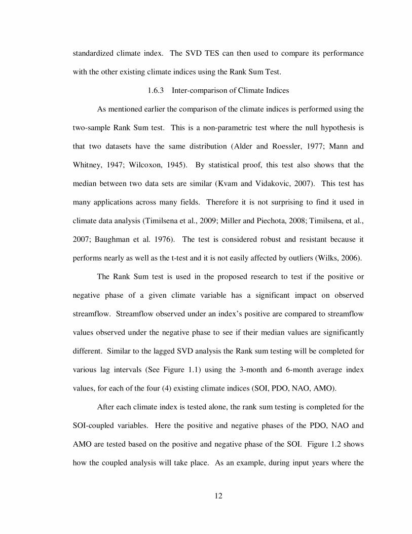
Figure 1.1 Depiction of 3-month and 6-month lag-lead analysis ................................. 11
Figure 1.2 Combination rank sum testing using the SOI as a basis .............................. 13
Figure 1.3 Depiction of extended 3-month analysis of climate data ............................ 15
Figure 2.1 Mean SOI values 1951-2009 (monthly-grey / yearly-black) ....................... 26
Figure 2.2 Mean PDO values 1950-2007 (monthly-grey / yearly-black) ..................... 28
Figure 2.3 Mean NAO values 1950-2009 (monthly-grey / yearly-black) ..................... 31
Figure 2.4 Mean AMO values 1950-2009 (monthly-grey / yearly-black) .................... 33
Figure 2.5 60S -60N ERSST Annual Anomaly (1880 – 2009) .................................... 35
Figure 2.6 Location Map showing the limits of the SST data. ..................................... 37
Figure 2.7 Location map of 29 USGS streamflow gauges ........................................... 41
Figure 3.1 Location map of 29 USGS streamflow gauges ........................................... 49
Figure 3.2 Depiction of 3-month and 6-month lag-lead analysis ................................. 51
Figure 3.3 Combination rank sum testing using the SOI as a basin ............................. 53
Figure 3.4 Number of significant results of the rank sum test ..................................... 59
Figure 3.5 6-month left and right heterogeneous correlation maps (|r| ≥ 0.27) ............. 61
Figure 3.6 3-month left and right heterogeneous correlation maps (|r| ≥ 0.27) ............. 62
Figure 3.7 Plots showing contribution of index to forecast skill. ................................. 66
Figure 4.1 Location map of 29 USGS streamflow gauges ........................................... 71
Figure 4.2 Lagged analysis schematic ........................................................................ 73
Figure 4.3 0-year and 1-year lag correlation maps from SVD analysis ........................ 75
Figure 4.4 2-year and 3-year lag correlation maps from SVD analysis ........................ 76
Figure 4.5 0-year and 1-year Z500 correlation maps ................................................... 79
Figure 4.6 2-year and 3-year Z500 correlation maps ................................................... 80
Figure 4.7 0-year and 1-year U200 correlation maps .................................................. 81
Figure 4.8 2-year and 3-year U200 correlation maps .................................................. 82
Figure 4.9 Zonal wind field (a) and sea level pressure (b) climatology maps. ............. 84
Figure 4.10 Comparison between 1983 and 2003 ENSO Events ................................... 86
Figure 5.1 Location map of 29 USGS streamflow gauges ........................................... 96
Figure 5.2 Schematic showing how Pf and Po are obtained from the eCDF ............... 103
Figure 5.3 Maps showing average skill score results. ................................................ 108
Figure 5.4 Scatterplots from Alternative 2 (Observed vs. Forecast) .......................... 110
Figure 5.5 Scatterplots from Alternative 3 (Observed vs. Forecast) .......................... 111
Figure 5.6 0-year lag forecast relative errors for eight gauge locations...................... 112
Figure 5.7 1-year lag forecast relative errors for eight gauge locations...................... 113
Figure 5.8 2-year lag forecast relative errors for eight gauge locations...................... 114
1
CHAPTER 1
INTRODUCTION
1.1 Research Problem
This dissertation seeks to improve the quality and length of lead time used in
ensemble forecasts of streamflow. The basic concept of ensemble forecasting can be
explained as the use of some initial states (observed climate data) being applied as input
into numerical weather models which simulate climate patterns. The process produces
various model outputs, or traces, which are the result of answering the question: what
would have happened in the past if the current initial conditions had been present? The
number of traces created by the ensemble forecast model produces a probability
distribution of time series data, from which, the mean trace or 95% confidence limits can
be extracted.
The use of ensemble forecasting has been developing for several decades.
Gleeson (1961, 1970) introduced the concept of defining the probability space of a given
climate field while using quantum mechanics and statistical mechanics to define a final
distribution, or ensemble, of forecast values. Epstein (1969) also provided some
theoretical and practical approaches to handle the issue of uncertainty in numerical
weather prediction (NWP) forecasts. However, the theoretical equations proved to be
extremely complicated and still were not capable of capturing enough of the atmospheric
uncertainty to generate a reliable forecast. Building upon this research Leith (1974)
proposed and tested the skill of approximating the stochastic dynamic forecasting
technique introduced by Epstein by using Monte-Carlo methods. Since Monte-Carlo

2
methods are used to generate ensemble forecasts, the improvement in computing
resources has automatically improved the frequency and quality of the forecasts.
In the short term (3 – 7 days) ensemble forecasts have demonstrated good
accuracy, but more importantly, the uncertainty of these forecasts is fairly well known.
Once there is a shift from short-term to mid-term (10 – 30 days) forecasts, as well as
long-term forecasts (monthly – seasonal) the significant autocorrelation of the climate
states is eliminated and the model becomes heavily dependent upon the accuracy of the
initial condition’s estimate and the NWP model (Wilks, 2006).
1.2 Long Lead Ensemble Streamflow Forecasting
The use of ensemble forecasts for climate forecasts is virtually the same for
making streamflow forecasts, except that streamflow forecasts require a hydrologic
modeling component to convert the forecasted temperature and precipitation data into
surface runoff or snow pack. Therefore the first step to increasing the forecast lead time
is to incorporate knowledge of how the volume of water stored as snowpack contributes
to runoff in the spring. Whether using an ensemble streamflow forecasting technique or
not, understanding the relationship between a basin’s snowpack and spring runoff can
extend the forecast lead time (Miller et al, 2006; Grantz et al., 2005; Simpson et al., 2004;
Cayan and Peterson, 1989).
A second method to extending streamflow forecast lead times is to utilized
climate data which demonstrates interannual, or even interdecadal persistence. In this
scenario, a climate event must have the ability to remain in an anomalous phase
(observations which are significantly higher or lower than the expected seasonal values)
for much longer than the forecast lead time. There are many climate indices that have

3
been defined to represent persistent climate variability including the Pacific Decadal
Oscillation (PDO), El Niño Southern Oscillation (ENSO), North Atlantic Oscillation
(NAO) and the Atlantic Multi-decadal Oscillation (AMO). While the discussion of how
each of these climate indices has been used in research is given in Chapter 2, it is
important to point out that this list is not exhaustive, nor is it impossible to expect that
there are other climate patterns not currently defined by a climate index which may
improve long-lead forecasts.
1.3 Water Resource Planning Forecasts in the Colorado River Basin
For stakeholders of the Colorado River Basin (CRB), having a better estimate of
the streamflow before the spring runoff begins is necessary for them to make effective
water management decisions. Water resource projection generated prior to a given water
year are typically heavily dependent upon the historical average of runoff for the CRB, or
historically ambivalent water-year outlooks which are modeled assuming all input years
have equally probable impact on the coming year’s streamflow. In order to assist water
managers of the CRB, the National Weather Service’s (NWS) Colorado Basin River
Forecast Center (CBRFC) issues three different types of forecasts.
The first CBRFC water supply forecast is a 3-month forecast of monthly water
volumes issued at the start of each month throughout the year. The second forecast is a
4-month lump sum water volume for the April – July runoff period. This forecast is
issued starting January 1 of each year and updated monthly through July 1. The final
forecast is actually referred to only as an “outlook” for the coming water year. While this
water-year outlook is generated using the same tool as the April – July forecast, there is
less confidence in the output value for several reasons, including: lack of research

4
supporting 12-month forecasts, and unknown uncertainty in the model. The outlook is
issued on August 1 and then updated on October 1 (NWS CBRFC staff, personal
communication, 2008).
All three forecasts are generated using the same analysis tool: the Extended
Streamflow Prediction (ESP) software (Day, 1985). ESP forecasts are calibrated on the
observed soil moisture, climate (Temperature and Precipitation) and runoff data from the
30 period of 1976-2005. The observed soil moisture conditions and snowpack
measurements (if available) are used as the initial conditions for the ESP model. The
ESP uses the initial conditions and creates a time series of daily streamflow values (also
known as a “trace”) by applying a time series of temperature and precipitation values
from a year in the calibration period (e.g. 1976). In all, the ESP analysis creates 30
output traces: one for each calibration year. From these 30 values, the median is reported
as the forecast value, and the 5th, 10th, 90th, and 95th quartiles are reported as different
confidence intervals (NWS CBRFC staff, personal communication, 2009).
The April – July forecast is unique in that it is created in coordination with the
National Resource Conservation Service (NRCS) who generate their own forecast for the
runoff season (April-July) each year. Before the CBRFC forecast is officially issued to
the CRB stakeholders, CBRFC and NRCS staff meet to discuss their separate forecast
results before issuing the “coordinated” runoff forecast for the CRB (NWS CBRFC staff,
personal communication, 2008).
After the ESP generates its forecast traces certain years can be assigned more
significance than others based on climatic similarities between the forecast year and the
calibrated historical years. Research related to finding a post-analysis weight method has
5
been done on the April – July forecasts while using the average November – January
Niño3.4 index as a predictor of seasonal streamflow (Werner et al, 2004). Werner et al.
were able to define a weighting technique for the April – Forecasts created by the ESP at
two locations within the CRB, but because of the poor El Niño Southern Oscillation
(ENSO) impact in the northern regions of the basin, the weighting technique was,
predictably, non-significant. Also noticeably absent from this paper was any discussion
about how this research can improve forecasts (or outlooks) created more than a few
months ahead of the spring runoff. As such was the case, currently no research has been
done to improve the water-year outlook created by the ESP.
1.3.1 CRB Forecasts and the 24-Month Study
Whether it is the 3-month forecasts, the April – July forecast, or the water year
outlook, the forecast, and outlook, values are reported for a dozen locations in the upper
CRB. The USBR uses the ESP and ESP/NRCS forecasts to create a 24-month projection
of water resource storage and releases along the CRB by modeling the forecast inputs
through the river basin modeling tool, RiverWare. The 24-month study uses the ESP-
generated forecasts as the primary input into the RiverWare model for the first year of the
study. The second year of the study uses the 30-year average (1976-2005) observed
streamflow values to continue their release/storage projections based on the various
treaties, compacts, laws, and court decisions which make up the “Law of the River”. The
24-month study is then issued to all stakeholders of the Colorado River including fish and
wildlife, power generation and water consumption managers, all of whom use this
information in their operation plans (USBR staff, personal communication, 2009).
6
There are many studies which demonstrate the uses of the 24-month study with
respect to CRB water resources. Background information into computer models used to
manage storage and release schedules can be found in Schuster (1989), Fulp et al, (1991),
and Zagona et al, (2001). Most of the research regarding modeling of CRB streamflow
and the 24-month study, try to simulate policy decisions on future river conditions based
on using the Law of the River as constraints in the 24-month study (Stevens, 1986;
Booker, 1995; Sangoyomi and Harding, 1995; Fulp et al, 1991; Gilmore et al., 2000).
One study touched on the inputs and assumptions of the 24-month study (Garrick, et al,
2008). However, there are no studies which examine the quality of the 24-month study
inputs, or ways to improve them.
1.4 Existing CRB-Climate Teleconnections
Recent research has provided many tools for the climate scientist to understand
the connection between large-scale climate inputs (for example, sea surface temperatures
(SST) and sea level pressure) with surface climate over the United States (Ropelewski
and Halpert, 1986, 1989; Latif and Barnett, 1994; McCabe and Dettinger, 1999;
Rajagopalan et al., 2000; Hidalgo, 2004; McCabe et al., 2007). Due to the recent drought
conditions in the desert southwest, much of this research focuses on ways to describe the
changes Colorado River Basin (CRB) streamflow by observing large-scale climate
variability over the Pacific Oceans (Grantz et al., 2005; Kim et al. 2006; Kim et al. 2007).
The well known relationships between SST/SLP data and streamflow of the western
United States are attributed to the El Niño Southern Oscillation (ENSO). However, there
are limitations to what information the ENSO can provide water managers of the CRB
(McCabe and Dettinger, 2002).
7
The first limitation is that the effects of the ENSO, while easily correlated with
surface climate of the northwestern and southwestern areas of the United States
(Ropelewski and Halpert, 1986), has a poor signal over a large area covering central
California, Nevada, Utah, Colorado and Wyoming which does not respond consistently to
ENSO variability (Hidalgo and Dracup, 2003; Kahya and Dracup, 1993; Kahya and
Dracup 1994b). Clark et al. (2001) supposes that this region is a transition area between
the positive ENSO-Streamflow correlation of the southwest, and the negative ENSO-
Streamflow correlation of the northwest. Because of the focus on ENSO signals over
larger regions of the U.S., there is no research that shows if any other climate index
demonstrates significant correlation with the entire CRB.
Another limitation to the ENSO is that its effect on surface hydrology of the
western U.S. has a lead time which does not lend itself to improving the long-lead
forecasts used in the 24-month study. McCabe and Dettinger (2002), who tested a lagged
response between ENSO and snowpack in the upper Rocky Mountains, found that
summer-fall ENSO observations were correlated with snowpack measurements in the
western U.S. Since snowpack measurements are well correlated with spring runoff
(Clark et al., 2001), this provided the potential for forecasting the April – July runoff
about 7 months before the predictand period. In order to improve the ESP outlook the
research needs to show a relationship between the entire water year (October –
September and not just April – July) volume, and the months leading up to that year.
There are no studies which examine the limit of the lag response between the established
climate indices and CRB streamflow.

8
1.5 Research Questions
The overall goal of the proposed research is to develop an approach which is
capable of improving the existing ESP outlook by establishing a weight methodology that
will be applied to the ESP output to generate a new forecast. This goal is broken down
into the following three research questions:
Question 1: Which large-scale climate patterns demonstrate a long-lead
connection to most of the streamflow in the CRB?
Hypothesis 1: A 1-year lagged teleconnection will be identified, but it will most
likely not be associated with an established climate index.
Question 2: How does the Pacific Ocean climate impact streamflow in the
Colorado River Basin?
Hypothesis 2: The Pacific Ocean – CRB connection will be explained through
analysis of atmospheric data and demonstrate a significant
correlation with streamflow gauges in the CRB
Question 3: Which climate lag-time and weight technique combination
demonstrates the greatest potential for generating successful
forecasts?
Hypothesis 3: The optimal forecasting approach will improve upon the use of
climatology as a forecast value and provide a basis for testing the
ESP output

9
1.6 Research Tasks – Question 1
1.6.1 Establishing a Long Lead Climate-Streamflow Teleconnection
Question No. 1: Which large-scale climate patterns demonstrate a long-lead connection
to most of the streamflow in the CRB?
The most well understood atmospheric or oceanic patterns used in research
include the El Niño Southern Oscillation (ENSO) as represented by the Southern
Oscillation Index (SOI), the Pacific Decadal Oscillation (PDO), the Northern Atlantic
Oscillation (NAO), and the Atlantic Multidecadal Oscillation (AMO). While there are
many more climate indices representing different areas of the globe, these four are most
often used in research when trying to define Climate-Hydrology teleconnections.
Therefore these climate indices will form the foundation of the first question. Aside from
the existing climate indices an SST index will be “created” for the CRB and then
compared to the other established climate indices. All of the teleconnections are
established using the climate data from a given water year with the streamflow volumes
of the following water year. A full description of the data and the origin of each data set
is given in Chapter 2.
The first step to find an answer to the first question is summarized into the
following tasks:
1a) Define an SST region of the Pacific Ocean using Singular Value Decomposition
(SVD).
1b) Compare the existing climate indices with the SVD results using Rank Sum
testing

10
1c) Assess the forecast potential of the results from (1a) and (1b) by creating a sample
forecast using a weighted kernel approach to optimize forecast skill score.
1.6.2 Defining the SST-Streamflow Teleconnection
Yarnall and Diaz (1986) suggested the potential to create basin-specific indices.
In light of the suggestion, the basic concept of Singular Value Decomposition (SVD) is
to provide an understanding of the covariance between two spatially distributed datasets
(Prohaska, 1976). Therefore the application of this method can work for finding the
contribution of one data field upon another, so long as the have the same number of
observations. Since this is the case the application of this method has appeared widely in
research whose aim is to describe the covariance of two meteorological data sets
(Oikonomou et al., 2010; Grassi et al., 2009; Yang, 2009; Wu et al., 2007; Skinner et al.,
2006; Tootle and Piechota, 2006; Xue et al., 2005; Shabbar and Skinner, 2004; Kim et
al., 2002; George and Saunders, 2001; Cholaw and Liren, 1999; Nakamura, 1996). The
utility of SVD was compared to other analysis techniques by Bretherton et al. (1992) and
its companion paper Wallace et al. (1992). In general, SVD is ideal for climate analysis
because it provides a non-parametric explanation of the climatic contribution of one
dataset on another.
The use of SVD in the proposed work will use the 3-month average and 6-month
average SST values of a 2º SST grid from 120º East to 80º West and 20º South to 60º
North. These two monthly averages are chosen arbitrarily, but they are intended to
reflect a season, or two seasons, of SST data. SVD analysis is run for various lag times
to find the optimal long-lead lag time. Figure 1.1 shows how each lag time will be tested.
Since the goal is to improve the forecasts for the following water year, the initial lag time

11
Figure 1.1 Depiction of 3-month and 6-month lag-lead analysis (Qi = yearly total runoff measured at station i)
(lag 0) is the July-September SST average and the April – September SST average for the
3-month and 6-month analyses respectively. Therefore, Lag 1 is the June-August SST
average and March-August SST average for the 3-month and 6-month analyses
respectively. Each lag represents a one month step back in time, and there are lags
generated until reaching the start of the previous water year (for example October-
December for the 3-month, lag 9; and October-March for the 6-month, lag 6).
The output of the SVD analysis will be mapped to show regions where the
covariance is significant (α = 0.05) between the SST gird location and a given streamflow
gauge in the CRB. These maps will help identify a specific region which represents the
strongest covariance with CRB streamflow. In addition to the maps the SVD also
provides a Temporal Expansion Series (TES) which resembles the properties of a
12
standardized climate index. The SVD TES can then used to compare its performance
with the other existing climate indices using the Rank Sum Test.
1.6.3 Inter-comparison of Climate Indices
As mentioned earlier the comparison of the climate indices is performed using the
two-sample Rank Sum test. This is a non-parametric test where the null hypothesis is
that two datasets have the same distribution (Alder and Roessler, 1977; Mann and
Whitney, 1947; Wilcoxon, 1945). By statistical proof, this test also shows that the
median between two data sets are similar (Kvam and Vidakovic, 2007). This test has
many applications across many fields. Therefore it is not surprising to find it used in
climate data analysis (Timilsena et al., 2009; Miller and Piechota, 2008; Timilsena, et al.,
2007; Baughman et al. 1976). The test is considered robust and resistant because it
performs nearly as well as the t-test and it is not easily affected by outliers (Wilks, 2006).
The Rank Sum test is used in the proposed research to test if the positive or
negative phase of a given climate variable has a significant impact on observed
streamflow. Streamflow observed under an index’s positive are compared to streamflow
values observed under the negative phase to see if their median values are significantly
different. Similar to the lagged SVD analysis the Rank sum testing will be completed for
various lag intervals (See Figure 1.1) using the 3-month and 6-month average index
values, for each of the four (4) existing climate indices (SOI, PDO, NAO, AMO).
After each climate index is tested alone, the rank sum testing is completed for the
SOI-coupled variables. Here the positive and negative phases of the PDO, NAO and
AMO are tested based on the positive and negative phase of the SOI. Figure 1.2 shows
how the coupled analysis will take place. As an example, during input years where the
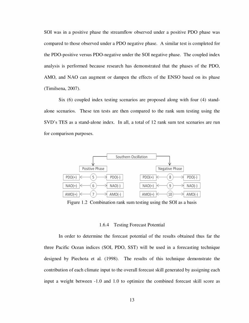
13
SOI was in a positive phase the streamflow observed under a positive PDO phase was
compared to those observed under a PDO negative phase. A similar test is completed for
the PDO-positive versus PDO-negative under the SOI negative phase. The coupled index
analysis is performed because research has demonstrated that the phases of the PDO,
AMO, and NAO can augment or dampen the effects of the ENSO based on its phase
(Timilsena, 2007).
Six (6) coupled index testing scenarios are proposed along with four (4) stand-
alone scenarios. These ten tests are then compared to the rank sum testing using the
SVD’s TES as a stand-alone index. In all, a total of 12 rank sum test scenarios are run
for comparison purposes.
Figure 1.2 Combination rank sum testing using the SOI as a basis
1.6.4 Testing Forecast Potential
In order to determine the forecast potential of the results obtained thus far the
three Pacific Ocean indices (SOI, PDO, SST) will be used in a forecasting technique
designed by Piechota et al. (1998). The results of this technique demonstrate the
contribution of each climate input to the overall forecast skill generated by assigning each
input a weight between -1.0 and 1.0 to optimize the combined forecast skill score as
14
determined by the Linear Error in Probability Space (LEPS) score (more details about the
LEPS score are provided below).
1.7 Research Tasks – Question 2
Question No. 2: How does the Pacific Ocean climate impact streamflow in the Colorado
River Basin?
Since the analysis from Task 1 may solely be a statistical relationship, it is
necessary to analyze further the physical connection linking Pacific Ocean Climate with
Colorado River Streamflow. To accomplish this goal the following subtasks are
proposed:
2a) Use SVD on datasets which represent atmospheric climate fields such as zonal
wind, geopotential height, and/or sea level pressure to identify the physical
connection between Pacific Ocean SSTs and CRB streamflow
2b) Compare the SVD analysis to current research into Pacific Ocean teleconnections
with the intermountain west to identify common patterns between the proposed
work and other research
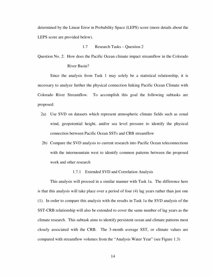
1.7.1 Extended SVD and Correlation Analysis
This analysis will proceed in a similar manner with Task 1a. The difference here
is that this analysis will take place over a period of four (4) lag years rather than just one
(1). In order to compare this analysis with the results in Task 1a the SVD analysis of the
SST-CRB relationship will also be extended to cover the same number of lag years as the
climate research. This subtask aims to identify persistent ocean and climate patterns most
closely associated with the CRB. The 3-month average SST, or climate values are
compared with streamflow volumes from the “Analysis Water Year” (see Figure 1.3)
15
Figure 1.3 Depiction of extended 3-month analysis of climate data
The SVD on the SST – Streamflow covariance matrix gives three matrices
[SVD(covarTS) = U Σ V], where V represents the decomposed covariance values closely
associated with the streamflow. Therefore, given the decomposed matrix, V, and the
original matrix of streamflow anomalies, S, the streamflow temporal expansion series
(STES) is determined by the following equation: STES = V’S’. The result of this
calculation is a series of values, one for each time period in V and S. Once calculated, the
STES is then correlated with cell of the Z500 and U200 gridded data.
1.7.2 Comparison With Current Research
There are several studies by Wang et al. (2009, 2010a, 2010b, 2010c) that are
significant to the proposed work trying to establish a connection between the Pacific
Ocean and CRB Streamflow. These studies represent an analysis of the long-lead
climate drivers of precipitation in the intermountain west region of the U.S. The reason
these studies are of importance to the proposed work is that they identify the physical
relationship between the Pacific Ocean cycles and the lagged response in precipitation.
According to several studies (Ely et al. 1994; Harnack et al., 1998; Schafer and
Steenburgh 2008) the precipitation in the intermountain west is typically produced by
transient synoptic activity (i.e. cyclone waves and the interaction of frontal passages with
16
orography - the spatial variation in the atmosphere). Wang et al (2009) identified that the
Pacific Ocean SSTs have a 10-20 year cycle, and that this cycle leads a precipitation
cycle of similar length by about 3-years. Wang et al (2010a) show that the Pacific Ocean
cycles are actually closer to 12 years and are best represented by the central equatorial
region of SSTs (essentially the Niño4 region: 5˚N-5˚S and 160˚E-150˚W). This study
analyzed the water vapor flux data in order to identify the leading modes of the transient
synoptic activity impacting the intermountain west. The results of this analysis showed
that there is a 3-year lag between the first two principle components of the moisture flux
data, and the first component is highly correlated with the Niño4 data and the second
component is highly correlated with the precipitation cycle.
The work of Wang et al (2010c) analyzed the moisture flux potential data to
determine the specific mechanism drawing storm activity into the intermountain west
region. The second mode of the principle component analysis revealed the t short
atmospheric wave pattern beginning in western tropical region (east of the Philippines)
and ending off the coast of the pacific Northwest coast of the U.S. this wave track is the
primary driver of the persistent climate anomalies toward the western U.S.
The works by Wang et al provide the proposed work with a foundation upon
which to build. The circulation patterns and leading cycles identified will provide a basis
for understanding the results generated in the proposed work. For example since the
foundation identifies a 3-year lag time between Pacific Ocean SSTs and the precipitation
in the intermountain west, then the proposed analysis should resemble this lag time as
well. Also since the short wave track identifies several region of significance between

17
the tropical pacific and the western U.S. the proposed research should identify at least
one of these regions as significant in the SVD analysis.
1.8 Research Tasks – Question 3
Question No. 3: Which climate lag-time and weight technique combination demonstrates
the greatest potential for generating successful forecasts?
Building upon the results from the first question the approach to the second
question is broken down into the following tasks:
3a) Calculate probability weights for years based on the three most significant SST
regions identified in Task 1b using four (4) weighting kernels
3b) Assess forecast skill of kernel-interval input combination using weighted
bootstrap technique to create a cross validation forecast for CRB streamflow from
1976-2005
3c) Using the best weight kernel-interval input combination from Task 2b, re-forecast
streamflow for 1906 – 1974
1.8.1 Weight Kernel Selection
Four different kernels are selected to create forecast values. The kernel which
results in the highest improvement in forecast skill is considered the optimal choice. The
first weight kernel is taken from research by Rajagopalan and Lall (1999) which is used
in a k-Nearest Neighbor (k-NN) technique to downscale climate data from yearly
observations to daily data. The kernel is defined as follows:
1
1/1
1/
ii n
i
i
RW
R=
=
∑
18
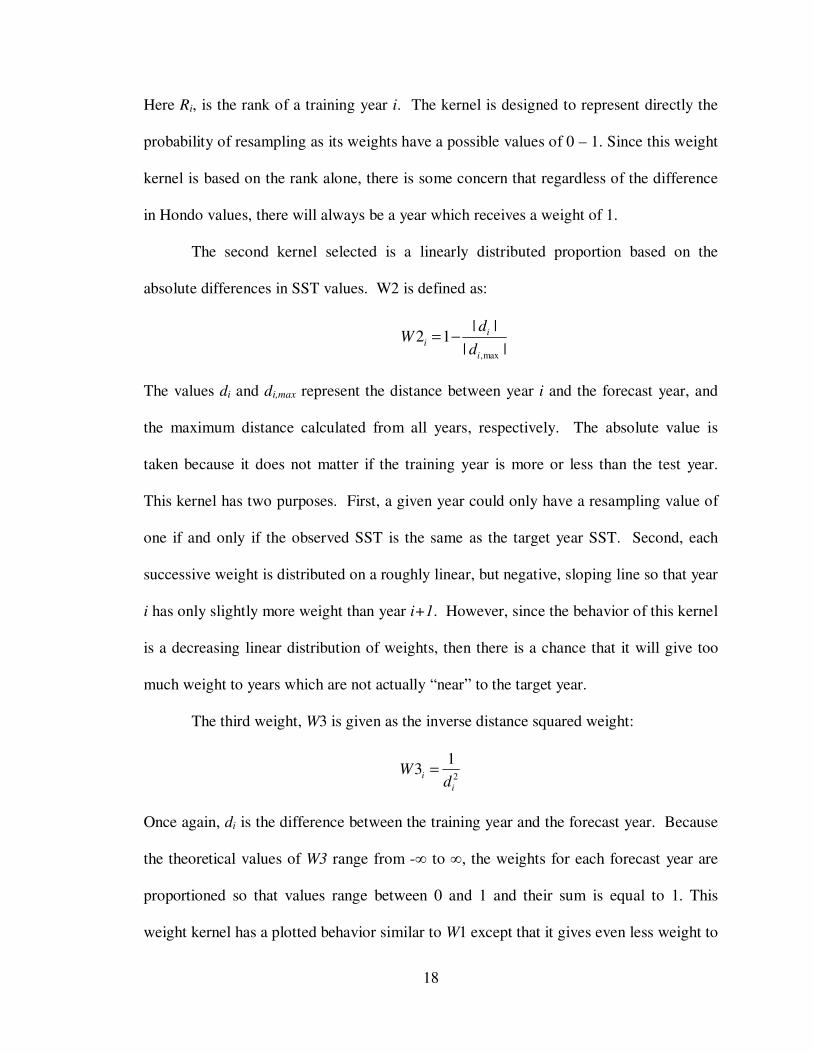
Here Ri, is the rank of a training year i. The kernel is designed to represent directly the
probability of resampling as its weights have a possible values of 0 – 1. Since this weight
kernel is based on the rank alone, there is some concern that regardless of the difference
in Hondo values, there will always be a year which receives a weight of 1.
The second kernel selected is a linearly distributed proportion based on the
absolute differences in SST values. W2 is defined as:
,max
| |2 1
| |i
i
i
dW
d= −
The values di and di,max represent the distance between year i and the forecast year, and
the maximum distance calculated from all years, respectively. The absolute value is
taken because it does not matter if the training year is more or less than the test year.
This kernel has two purposes. First, a given year could only have a resampling value of
one if and only if the observed SST is the same as the target year SST. Second, each
successive weight is distributed on a roughly linear, but negative, sloping line so that year
i has only slightly more weight than year i+1. However, since the behavior of this kernel
is a decreasing linear distribution of weights, then there is a chance that it will give too
much weight to years which are not actually “near” to the target year.
The third weight, W3 is given as the inverse distance squared weight:
2
13i
i
Wd
=
Once again, di is the difference between the training year and the forecast year. Because
the theoretical values of W3 range from -∞ to ∞, the weights for each forecast year are
proportioned so that values range between 0 and 1 and their sum is equal to 1. This
weight kernel has a plotted behavior similar to W1 except that it gives even less weight to

19
observations with increasing values of di. Since this kernel does shift the majority of the
weight to the first or second years some relevant information from other years may be
ignored.
The final kernel, W4 is simply the inverse distance:
14i
i
Wd
=
Both W3 and W4 are commonly used kernels used in resampling and interpolating
applications or as comparisons to other more sophisticated methods. W4 does not weigh
the closest 1 or 2 as heavily as W1 or W3, but since it is not linear it also does not
distribute the weights to too many of the other, adjacent observations.
Weights are calculated using the raw SST values. A test was run to see if there
would be any difference between using raw data and calculating the Hondo anomalies
which were used in the SVD analysis (Lamb et al. 2010, Aziz et al,. 2010). The results of
this simple test demonstrated that there was no significant difference between the forecast
skill score resulting from these two data sets. Additionally, using proportioned weights
were compared to raw (un-proportioned) weights to see if the forecast skill is sensitive to
either method. The results of this test demonstrated that there was no significant
difference. From these two small tests the use of the raw Hondo data is selected for
testing because it is simpler to employ, and the proportioned weights are used because
they communicate the idea of resampling probability better than the raw weights.
The weighting kernels determine resampling probabilities for each of the 30 years
in the analysis period. Since these are being applied to 30 years in the cross-validation
analysis, a 30 x 30 matrix of values is created from a given weight kernel. Once matrix
of probabilities is created for each weight kernel selected. Since the weight kernels are

20
also based on which 3-month average SST values are used (i.e. Dec-Feb, Jan-Mar, or
Feb-Apr) a total of 12 probability matrices are calculated to generate the forecasts for
Task 2b.
1.8.2 Cross-Validation Forecast Skill
Using the results from 2a, the forecasts are generated for each kernel-SST
interval. This is done using a weighted bootstrap technique. The bootstrap technique
was first developed by Efron (1979, 1982) in order to make estimates of population
parameters from relatively small datasets. This method is selected because it, like the
other statistical methods proposed in this research, is non-parametric. The current
research proposed using the weighted (or generalized bootstrap) method to intentionally
introduce a bias to the resampling process (Barbe and Bertail, 1995).
In order to preserve the ~1 year lag between the Pacific Ocean SST region and the
streamflow observations the probability weights are actually calculated on the data set
from 1975-2004, and then applied to the observed data from 176-2005. The 30 year
period from 1976-2005 is significant because this is the current 30 period upon which the
CBRFC ESP model is calibrated. Using this 30-year period will provide a better basis for
comparison in future research tasks.
The forecast skill score is determined using the Linear Error in Probability Space
(LEPS) score. This score was initially developed by Ward and Folland (1991) and
further revised by Potts et al. (1996). The score measures the distance between the
observed and forecast values in probability space. To do this the LEPS score requires
that an empirical distribution function (EDF) be created for each streamflow gauge. The

21
probabilities for the observed and forecast values are read from the appropriate EDF and
then inserted into the following equation developed by Potts et al.:
2 23(1 | | ) 1f o f f o vLEPS P P P P P P= − − + − + − −
After the forecast skill is calculated at each location for each year in the cross-
validation analysis, the average skill score is determined for each location in the CRB.
The average skill score is ranges from -1 to 1 with a score of 0 being as good as
forecasting with the mean. Scores which are greater than 10% are considered as “good”
skill. These results will help determine which weight kernel, applied to which 3-month
average SST interval, was most successful.

22
CHAPTER 2
LITERATURE REVIEW
2.1 Introduction
The proposed dissertation is based upon several general topics, which include
long-lead streamflow forecasting and the data typically used in such forecasting The
following chapter describes the basis of research regarding the recent improvements to
long-lead forecasting as well as the state of knowledge surrounding the data, which
include the Southern Oscillation Index (SOI – measure of the ENSO signal), Pacific
Decadal Oscillation (PDO), Atlantic Multi-decadal Oscillation (AMO), and North
Atlantic Oscillation (NAO) datasets. Also included in the proposed research is sea
surface temperature data, the naturalized/unimpaired streamflow data, and the historic
forecast data.
2.2 Streamflow Forecasting
As noted in Chapter 1, the major goal of the proposed dissertation is to improve
upon the current knowledge of long lead streamflow forecasting. For many years,
deterministic forecasts generated by understanding the relationship between snowpack
and spring runoff provided the only methodology to long-term streamflow forecasting
(Druce, 2001). In 1975 the Hydraulic Research Laboratory of the NWS in initiated a
program to create the Extended Streamflow Prediction (ESP) procedure. Day’s (1985)
work essentially marked the beginning of ensemble streamflow forecasting procedures
even though it did not wholly supplant any other forecasting method then or since (e.g.
Krzysztofowicz,1999; Kalra and Ahmad, 2009).
23
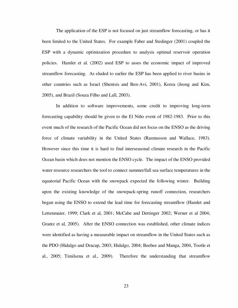
The application of the ESP is not focused on just streamflow forecasting, or has it
been limited to the United States. For example Faber and Stedinger (2001) coupled the
ESP with a dynamic optimization procedure to analysis optimal reservoir operation
policies. Hamlet et al. (2002) used ESP to asses the economic impact of improved
streamflow forecasting. As eluded to earlier the ESP has been applied to river basins in
other countries such as Israel (Shentsis and Ben-Avi, 2001), Korea (Jeong and Kim,
2005), and Brazil (Souza Filho and Lall, 2003).
In addition to software improvements, some credit to improving long-term
forecasting capability should be given to the El Niño event of 1982-1983. Prior to this
event much of the research of the Pacific Ocean did not focus on the ENSO as the driving
force of climate variability in the United States (Rasmusson and Wallace, 1983).
However since this time it is hard to find interseasonal climate research in the Pacific
Ocean basin which does not mention the ENSO cycle. The impact of the ENSO provided
water resource researchers the tool to connect summer/fall sea surface temperatures in the
equatorial Pacific Ocean with the snowpack expected the following winter. Building
upon the existing knowledge of the snowpack-spring runoff connection, researchers
began using the ENSO to extend the lead time for forecasting streamflow (Hamlet and
Lettenmaier, 1999; Clark et al, 2001; McCabe and Dettinger 2002; Werner et al 2004;
Grantz et al, 2005). After the ENSO connection was established, other climate indices
were identified as having a measurable impact on streamflow in the United States such as
the PDO (Hidalgo and Dracup, 2003; Hidalgo, 2004; Beebee and Manga, 2004, Tootle et
al., 2005; Timilsena et al., 2009). Therefore the understanding that streamflow

24
forecasting could take place well in advance of the spring runoff season became a
commonly accepted idea by the start of the last decade.
It should be pointed out here that the ESP tool and the use of large scale climate
as predictors in long-term streamflow forecasting, have largely been developed without a
comprehensive discussion about the model uncertainty (Krzysztofowicz,, 2001). Even
thought the ESP output is often communicated in terms of probability (e.g. median
forecast with 95% confidence limits), it does not discuss the sampling error imbedded in
the model’s initial states or the 30 calibrated years used to represent the population of
precipitation and temperature time series. ESP and large-scale climate uncertainty is a
large enough topic that it would warrant considerable work to fully address. However,
for completeness’ sake the limitations of the ESP are simply mentioned.
2.3 Pacific Ocean Climate Indices
Data from the Pacific Ocean has been logically linked with many hydrologic
responses in the world and especially in the United States, as is demonstrated below. The
two most widely used climate indices representing the Pacific Ocean include the
Southern Oscillation Index (SOI), representing the ENSO signal, and the Pacific Decadal
Oscillation (PDO). The SOI is a measurement of sea level pressure (SLP) and the PDO
is a measurement of sea surface temperatures.
2.3.1 El Niño Southern Oscillation
The ENSO is perhaps the most widely known climate variable outside of
academic circles. This acronym refers to both the warm and cool phases of the
oscillation known as El Niño and La Niña respectively. It was initially observed by Sir
Charles Todd, but not named, in the 1880’s, but it was ultimately defined by Sir Gilbert

25
Walker and his collaborators in publications in 1923 and 1932 as a “seesaw” of sea-level
pressure (Diaz and Markagraf, 1992). The increase in the South Pacific High diminishes
the tradewinds pushing east towards South America which results in warming SST’s. As
SST’s increase so does the evaporation and heating in the troposphere which improves
the conditions for “convection and rainfall” (Diaz and Markagraf, 1992).
Currently there are several indices used to define the ENSO phenomenon. These
indices include several sea surface temperature (SST) indices such as the Wright SST,
Niño1&2, Niño3, Niño3.4 and Niño4. In addition to the SST indices there is an index
created from sea level pressure (SLP), called the Southern Oscillation Index (SOI) and a
composite wind, pressure, and temperature index called the Multivariate ENSO Index
(MEI). Each has been used in various teleconnection studies and none is officially
accepted as the only index to represent the ENSO. Figure 2.1 shows a time series plot of
the SOI index from 1950 – 2010.
The proposed research uses the SOI to represent the ENSO which is maintained
by the National Oceanic Atmospheric Administration’s (NOAA) Climate Prediction
Center (CPC) and it can be downloaded from their website
(http://www.cpc.ncep.noaa.gov/data/indices/soi). The SOI dataset covers monthly values
from 1951 through the current year. The SOI is defined as the difference between the
standardized SLP anomalies at Tahiti and Darwin, Australia. These observations
describe the seesaw event that Walker (1923) and Walker and Bliss (1932) divide. As
SLP values increase in Darwin, there is a resulting decrease in SLP at Tahiti and vice
versa. Therefore a positive SOI phase occurs when the Tahitian SLP anomaly is greater
26
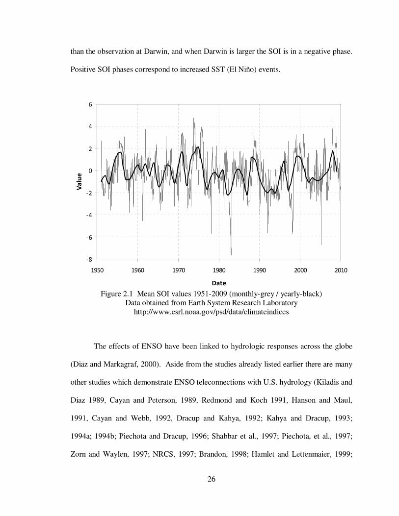
than the observation at Darwin, and when Darwin is larger the SOI is in a negative phase.
Positive SOI phases correspond to increased SST (El Niño) events.
-8
-6
-4
-2
0
2
4
6
1950 1960 1970 1980 1990 2000 2010
Date
Value
Figure 2.1 Mean SOI values 1951-2009 (monthly-grey / yearly-black)
Data obtained from Earth System Research Laboratory http://www.esrl.noaa.gov/psd/data/climateindices
The effects of ENSO have been linked to hydrologic responses across the globe
(Diaz and Markagraf, 2000). Aside from the studies already listed earlier there are many
other studies which demonstrate ENSO teleconnections with U.S. hydrology (Kiladis and
Diaz 1989, Cayan and Peterson, 1989, Redmond and Koch 1991, Hanson and Maul,
1991, Cayan and Webb, 1992, Dracup and Kahya, 1992; Kahya and Dracup, 1993;
1994a; 1994b; Piechota and Dracup, 1996; Shabbar et al., 1997; Piechota, et al., 1997;
Zorn and Waylen, 1997; NRCS, 1997; Brandon, 1998; Hamlet and Lettenmaier, 1999;

27
Schmidt et al., 2001; Harshburger et al., 2002; Maurer and Lettenmaier, 2003; Hidalgo
and Dracup, 2003; Hidalgo and Dracup, 2004; Beebee and Manga, 2004; Tootle and
Piechota, 2004; Mauer, et al., 2004; Hidalgo, 2004; Twine et al., 2005). Despite the
shortcomings of the ENSO already mentioned earlier, the ENSO-U.S. Hydrology
teleconnection has been discussed enough that is included here as a way to show that the
testing being done with the current research matches up with past research. It is expected
that the ENSO signal will appear during the short lag times and for gauges located in the
lower CRB. In the context of the current research, it is also expected to show the limit of
the ENSO-CRB teleconnection.
2.3.2 Pacific Decadal Oscillation
When discussing the CRB, the second most common climate index is the Pacific
Decadal Oscillation (PDO). The PDO is defined as the first mode of the principal
component analysis of Pacific Ocean SSTs poleward of 20º N. The anomalies and the
impacts of the PDO were initially observed by Nitta and Yamada (1989) and Trenbreth
(1990). PDO fluctuations have a period between 50-70 years with a given warm or cool
phase persisting for about 15 – 25 years (Chao et al., 2000; Minobe; 1997). The
mechanism driving PDO variability is not known, but it is hypothesized by Trenberth and
Hurell (1994), that the origins of the PDO can be found in the tropical Pacific Ocean.
PDO data are available from the Joint Institute for the Study of the Atmosphere and
Ocean at the University of Washington for the period of 1900 through the current year
(http://jisao.washington.edu/pdo/PDO.latest). Figure 2.2 shows a time series plot of the
PDO data.

28
-4
-3
-2
-1
0
1
2
3
4
1950 1960 1970 1980 1990 2000 2010
Date
Value
Figure 2.2 Mean PDO values 1950-2007 (monthly-grey / yearly-black)
Data obtained from Earth System Research Laboratory http://www.esrl.noaa.gov/psd/data/climateindices
Similar to the ENSO, the PDO teleconnection has been identified around the
Pacific Ocean basin. Studies showed symmetric atmospheric circulation changes
associated with the PDO (Gerreaud and Battisti, 1999; Zhang et al., 1997b). Power et al
(1997, 1999a, 1999b) showed how changes in the PDO impact Australian temperatures
and rainfall. However, a large number of studies demonstrate the impact the PDO has on
marine biology (Mantua and Hare, 2002; Hare et al., 1999; Beamish, 1993; McFarlane
and Beamish, 1992; Clark et al., 1999).
The climate impacts of the PDO have been shown to explain hydrologic
variability in the western U.S. under several different circumstances including ENSO-
29
PDO coupling (Minobe, 1997; Gershunov and Barnett, 1998; McCabe and Dettinger,
2002; Hidalgo and Dracup, 2003; Hidalgo, 2004; Beebee and Manga, 2004, Tootle et al.,
2005; Timilsena et al., 2009). In general, the PDO signal is often discussed in the context
of ENSO, because the PDO signal can either enhance or diminish the ENSO signal,
depending on the phase of the PDO (Hamlet and Lettenmaier, 1999). While there are
many studies which have discussed the impact of the ENSO, and the PDO, as well as the
ENSO-PDO effect on streamflow in the CRB, there is no study which defines the lagged
climate-hydrology response of these climate variables on the CRB.
2.4 Atlantic Ocean Climate Indices
The proposed research proposes to use Atlantic Ocean climate data to understand
the long-lead impacts associated with the CRB though there is significantly less research
connecting the two than with Pacific Ocean data. The two datasets selected for this work
include the Northern Atlantic Oscillation (NAO) and the Atlantic Multidecadal
Oscillation (AMO). However, Marshall et al (2001) point out that the North Atlantic
Ocean temperature and pressure variability can have an effect on weather throughout the
northern hemisphere. Because, as Marshall et al. point out, the NAO is a part of the
northern hemisphere circulation which is described by the Arctic Oscillation (AO). They
go on to demonstrate that the NAO/AO impacts can rival those of the ENSO signal from
the Pacific Ocean. Because of this information, there is a good reason to include Atlantic
Ocean climate data when considering streamflow responses in the CRB.
2.4.1 Northern Atlantic Oscillation
The NAO is defined as the anomaly differences in sea level pressure between the
Azores and Iceland (Hurell, 1995), and has also since been identified as part of northern

30
annular mode, the Arctic Oscillation (Marshall et al., 2001). Interestingly,
teleconnections identifying the NAO were made in the same studies that originally
identified the ENSO signal (Walker, 1924; Walker and Bliss, 1932). When in a positive
phase, the North Atlantic Jet moves poleward taking with it the storm track (Kushnir,
1994). Barnston and Livezey (1987) describe the NAO contracting northward in summer
and expanding southward in winter giving it a variable location which thought to be the
result of changes in North Atlantic SSTs (Kushnir et al., 2006). Unlike the ENSO and
PDO the NAO index does not remain in one phase for an extended period of time (See
Figure 2.3). Its short period of 12-14 days is the result of seasonal-to-interannual (S/I)
variability (e.g. affected by volcanic activity or internal dynamics of the climate system)
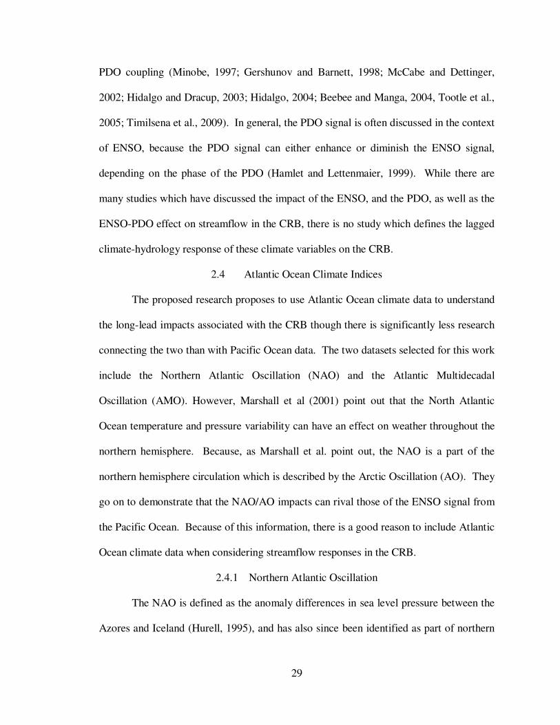
and is therefore nearly impossible to predict (Kushnir et al., 2006).
The NAO index is most famously teleconnected to climate in the northern
Atlantic Ocean (Visbeck et al. 2002; Kushnir 1994; Deser and Blackmon 1993; Wallace
et al. 1992; Bjerknes 1964). This basic understanding of changes in Atlantic SSTs has
led to many studies linking the NAO to hydrologic responses across Europe (Ionita et al.,
2009; Karcher et al., 2007; Macklin and Rumsby, 2007; Ukita et al., 2007; Otterson et al.,
2000; Frei and Robinson, 1999; Higuchi et al., 1999; Dugam et al., 1997; Nakamura,
1996; Hurell, 1995; Zhifang and Wallace, 1993; Van Loon and Rogers, 1978;). Other
studies have shown that this index can also explain variation in surface hydrology across
the United States. Morin et al. (2008) demonstrated that the primary mode of total
snowfall and number of snow days in the eastern United States is driven by the NAO.
Durkee et al. (2008) showed that there is an increase in precipitation across the eastern
United States when the NAO is in a positive phase. The use of positive and negative
31
phases of the NAO were also linked to changes in CRB streamflow by Tootle et al
(2005). Because the NAO is a measure of SLP, it is possible to describe the physical
connection of the index to changes in storm tracks across Europe. However no
explanation is given for the NAO – North American teleconnection.
-4
-3
-2
-1
0
1
2
3
4
1950 1960 1970 1980 1990 2000 2010
Date
Value
Figure 2.3 Mean NAO values 1950-2009 (monthly-grey / yearly-black)
Data obtained from Earth System Research Laboratory <http://www.esrl.noaa.gov/psd/data/climateindices>
2.4.2 Atlantic Multi-Decadal Oscillation
The AMO represents a persistent SST pattern observed in the northern Atlantic
Ocean between 0 – 70 degrees north bounded by the continents (Gray et al., 2004). In
contrast to the other indices discussed, the AMO does not vary drastically, and it is by far
the index with the longest cycle period. It is estimated from modeling studies to be 50-70

32
years, and from tree-ring and arctic ice regression as closer to 80 years (Schlesinger and
Ramankutty, 1994; Kerr, 2000). Figure 2.4 shows a time series plot of the AMO from
1950 – 2009. While the initial observation of the index may be attributed to Schlesinger
and Ramankutty, the definition of the AMO as an actual oscillation has largely come
from work aimed at extending the AMO through analysis of reconstructed SST datasets
(Gray et al., 2004; Knight et al., 2005). The increased understanding about the physics of
the AMO index (Dijkstra et al., 2006) comes from the studies which defined the
teleconnection of AMO and the Thermohaline Circulation (THC) (Sutton and Hodson,
2005; Knight et al., 2005; Dima and Lohman, 2007, Richter and Xie, 2009).
Understanding the AMO cycle has also helped understand the trends related to climate
change (Hodson, et al., 2009; Keenlyside et al., 2008).
Because the AMO index is also the youngest index there are fewer examples of
using this index in teleconnection studies. The AMO appears in research into
teleconnections with changes in Asian summer monsoons (Lu et al, 2006), Indian and
Sahal summer rainfall (Zhang and Delworth, 2006), northern Pacific Ocean variability
(Zhang and Delworth, 2007) and climate in east China (Shuaunglin and Bates, 2003).
Some of these teleconnections were also checked in the reconstructed AMO dataset
(Knight et al., 2006). Logically it also figures into research related to changes in
hurricane activity in the Atlantic Ocean and the resulting changes in precipitation in
countries adjacent to the Atlantic basin.
Goldenberg et al. (2001) used the AMO data to help explain the increase in
Atlantic Hurricane activity. Because of the longer trends of the AMO data, the study
concludes that the increased hurricane activity will persist for many years. Trenbreth and

33
Shea (2006) used the observed 2005 hurricane season as a backdrop to discuss the
observed increases in global temperature as a result of climate change and increases in
-1
-0.8
-0.6
-0.4
-0.2
0
0.2
0.4
0.6
0.8
1
1950 1960 1970 1980 1990 2000 2010
Date
Value
Figure 2.4 Mean AMO values 1950-2009 (monthly-grey / yearly-black)
Data obtained from Earth System Research Laboratory
http://www.esrl.noaa.gov/psd/data/climateindices
the AMO oscillation. Finally, Holland and Webster (2007), defined three regimes of
eastern Atlantic SSTs where there are 50% more cyclones and hurricanes in each
successive regime.
The connection between AMO and US streamflow has also been introduced in
studies showing changes in streamflow across the US, (Enfield et al., 2001), in Florida
(Kelley and Gore, 2008) and in gaining an understanding of long-term drought observed
in the southwest (Hidalgo, 2004). More pertinent to the current research the AMO-

34
ENSO coupled effect has appeared in studies looking at the Mississippi Valley
streamflow (Rogers and Coleman, 2003) as well as in the CRB (Timilsena et al, 2009,
Tootle et al, 2005). The AMO index data from 1948 through the present can be
downloaded from the CPC’s website (http://www.cdc.noaa.gov/Correlation/
amon.us.data).
2.5 Global Gridded Climate Data
In addition to using specific climate indices, the proposed research will use data
which is created for the entire globe and represented in a gridded format. These data
include Sea Surface Temperatures (SSTs), 500mb Geopotential Height (Z500), and
200mb Zonal wind (U200). The purpose of using the “raw” global data is to be able to
identify climate patterns which may not be represented in the defined climate indices
already listed
2.5.1 Sea Surface Temperature Data
The SST data used in the proposed research comes from work by Smith and
Reynolds (2002) at the National Climate Data Center (NCDC) of the National Oceanic
Atmospheric Administration (NOAA). Officially named the Extended Reconstructed Sea
Surface Temperature (ERSST) dataset, it comprises of monthly average values at 2-
degree grid cells covering the entire globe from 1854 – 1997. The dataset has been
improved (Smith and Reynolds 2004; Smith et al, 2008) since the initial reconstruction
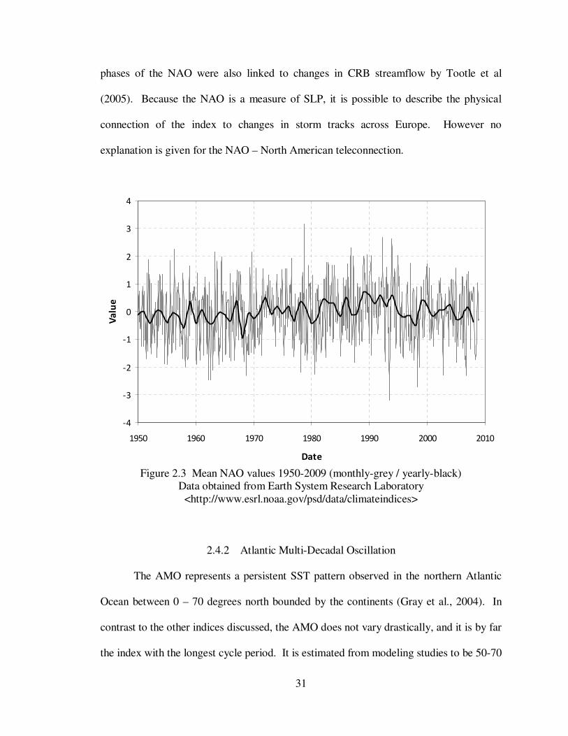
was performed to reduce bias and modeling error. Figure 2.5 shows the time series for
the mean SST values from 60° S – 60° N.
35
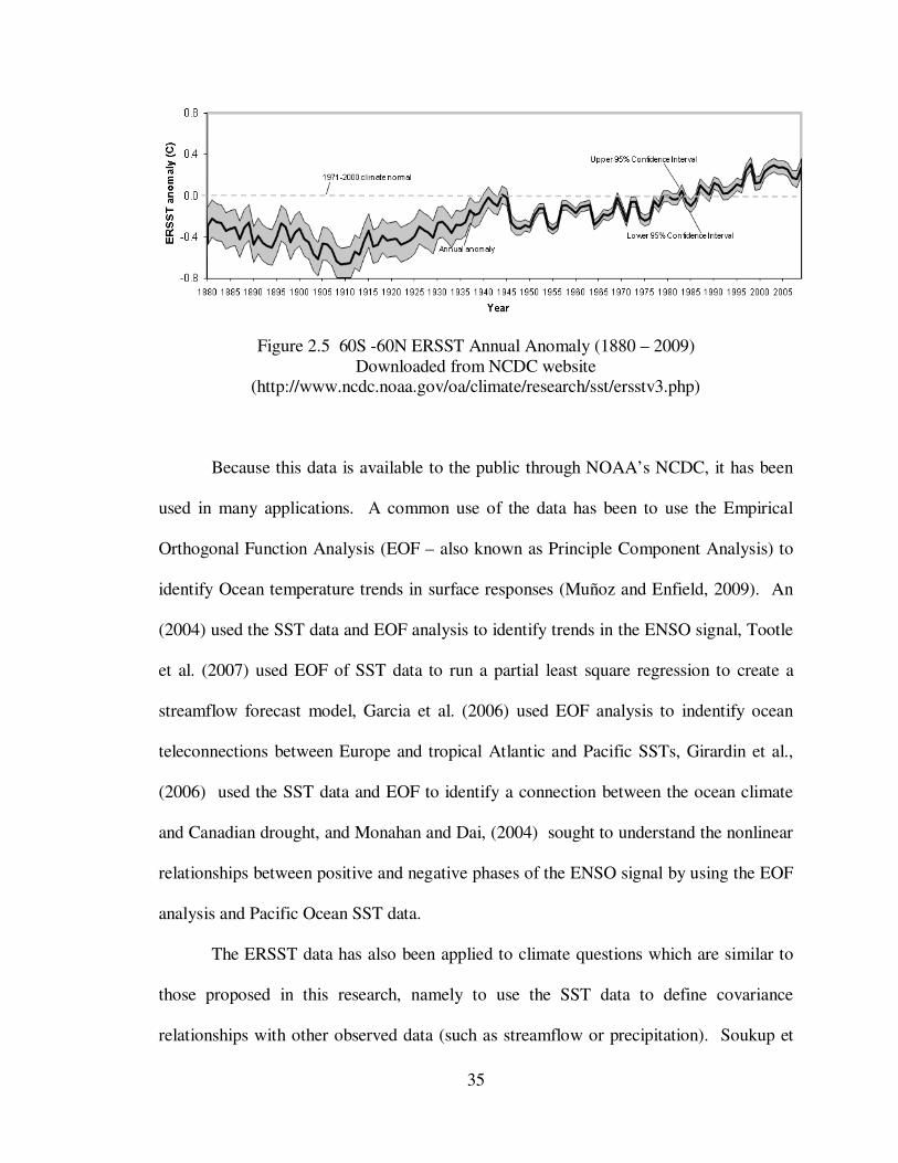
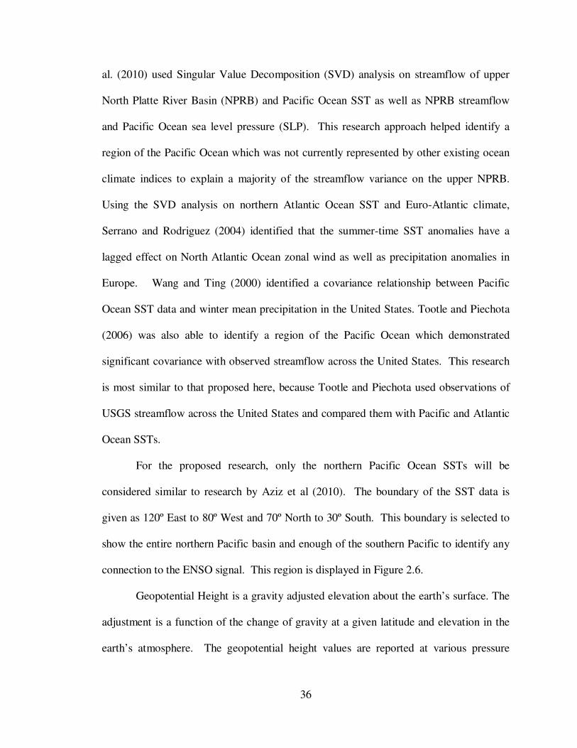
Figure 2.5 60S -60N ERSST Annual Anomaly (1880 – 2009) Downloaded from NCDC website
(http://www.ncdc.noaa.gov/oa/climate/research/sst/ersstv3.php)
Because this data is available to the public through NOAA’s NCDC, it has been
used in many applications. A common use of the data has been to use the Empirical
Orthogonal Function Analysis (EOF – also known as Principle Component Analysis) to
identify Ocean temperature trends in surface responses (Muñoz and Enfield, 2009). An
(2004) used the SST data and EOF analysis to identify trends in the ENSO signal, Tootle
et al. (2007) used EOF of SST data to run a partial least square regression to create a
streamflow forecast model, Garcia et al. (2006) used EOF analysis to indentify ocean
teleconnections between Europe and tropical Atlantic and Pacific SSTs, Girardin et al.,
(2006) used the SST data and EOF to identify a connection between the ocean climate
and Canadian drought, and Monahan and Dai, (2004) sought to understand the nonlinear
relationships between positive and negative phases of the ENSO signal by using the EOF
analysis and Pacific Ocean SST data.
The ERSST data has also been applied to climate questions which are similar to
those proposed in this research, namely to use the SST data to define covariance
relationships with other observed data (such as streamflow or precipitation). Soukup et
36
al. (2010) used Singular Value Decomposition (SVD) analysis on streamflow of upper
North Platte River Basin (NPRB) and Pacific Ocean SST as well as NPRB streamflow
and Pacific Ocean sea level pressure (SLP). This research approach helped identify a
region of the Pacific Ocean which was not currently represented by other existing ocean
climate indices to explain a majority of the streamflow variance on the upper NPRB.
Using the SVD analysis on northern Atlantic Ocean SST and Euro-Atlantic climate,
Serrano and Rodriguez (2004) identified that the summer-time SST anomalies have a
lagged effect on North Atlantic Ocean zonal wind as well as precipitation anomalies in
Europe. Wang and Ting (2000) identified a covariance relationship between Pacific
Ocean SST data and winter mean precipitation in the United States. Tootle and Piechota
(2006) was also able to identify a region of the Pacific Ocean which demonstrated
significant covariance with observed streamflow across the United States. This research
is most similar to that proposed here, because Tootle and Piechota used observations of
USGS streamflow across the United States and compared them with Pacific and Atlantic
Ocean SSTs.
For the proposed research, only the northern Pacific Ocean SSTs will be
considered similar to research by Aziz et al (2010). The boundary of the SST data is
given as 120º East to 80º West and 70º North to 30º South. This boundary is selected to
show the entire northern Pacific basin and enough of the southern Pacific to identify any
connection to the ENSO signal. This region is displayed in Figure 2.6.
Geopotential Height is a gravity adjusted elevation about the earth’s surface. The
adjustment is a function of the change of gravity at a given latitude and elevation in the
earth’s atmosphere. The geopotential height values are reported at various pressure

37
levels, and 500mb is simply one of those levels. Therefore the values used for this
research are reporting the additional amount of elevation required to “reach” elevation of
mean sea level. The geopotential height data are available from the NCEP/NCAR
Reanalysis Product (Kalnay et al, 1996), and can be downloaded from the following
website http://www.esrl.noaa.gov/psd/data/gridded/data.ncep.reanalysis.html. The 500mb
height data will identify circulation patterns in the upper layers of the atmosphere (above
land and sea). Therefore some studies use the data to identify teleconnection patterns or
atmospheric waves which demonstrate the path of storm tracks in the atmosphere (Mo
and White, 1985; Rogers, 1990; Thompson and Wallace, 1998; Yu, 2007).
Figure 2.6 Location Map showing the limits of the SST data.
(120º E – 80º W, 70º N to 30º S)

38
2.5.2 Geopotential Height
The utility of geopotential height as a climate variable is summarized by Wallace
and Gutzler (1981). Wallace and Gutzler used the data to reproduce these patterns and to
identify the Pacific/North American (PNA) signal as a teleconnection within the 500mb
geopotential height data. It is important to note that it was the sea level pressure data (a
subset of the geopotential height data) that Sir Gilbert Walker used initially to identify the
SOI as well as the NAO patterns. In general this dataset has been utilized so many times
that there is not enough room to list all of them here.
There are a few of the studies which relate to the tasks carried out in this research.
For example, work by Goebbert and Leslie (2010) identified a multi-year cycle present in
the geopotential height data in the northwest Australian tropical cyclone (TC) area. This
analysis showed there is a significant correlation between the wintertime climate variable
and the yearly TC frequency and the number of TC days each year. Casola and Wallace
(2007) showed the wintertime Z500 data is correlated with the ENSO signal in several
regions around the Pacific Basin and North America. Finally, work by Blackmon (1976)
helped set the foundation for using power spectrum analysis on the Z500 data to reveal
the low frequency signals imbedded in gridded climate data. These three studies show
that there is a low frequency cycle to the Z500 data which demonstrates noted
teleconnection patterns in the Pacific Basin and these have shown the potential for being
correlated with established climate phenomenon such as the ENSO cycle in the Rocky
Mountain region.
2.5.3 Zonal Wind Field
The atmospheric water budget is defined by Wang et al., (2010a) as the following.
39
W
Q E Pt
∂+ ∇ ⋅ = −
∂
Here, W, P, E, and Q represent respectively, precipitable water, precipitation, evaporation
and vertically integrated water vapor flux. Water vapor flux is defined as the integration
of specific humidity, q and zonal wind, V from the surface layer to the troposphere.
0
1 sp
Q qVdpg
= ∫
This demonstrates that the zonal wind field is a component of quantifying the
atmospheric budget. This zonal wind field, as a component in an atmospheric water
budget has been used specifically in research to connect the Pacific Ocean climate
variability to precipitation in the intermountain west (Wang et al., 2009, 2010a, 2010b).
This work uses both components of the water vapor flux as decomposed by Chen (1985),
namely the moisture flux streamfunction – a measurement of the amount of moisture
carried in the atmosphere – and the moisture flux potential.
The zonal wind field data has been used in studies as a climate variable itself.
Because it is also part of the NCEP/NCAR reanalysis product there are myriad research
examples using this data. The work by Athanasiadis (2010) used the wintertime 250 mb
zonal wind field to identify the location of the wintertime East Asian Jet Stream (EAJS)
and its correlation with north American storm tracks. Yang et al (2002) utilized the zonal
wind field data to draw between the variations of the EAJS and Asian-Pacific-American
winter climate. Zhang et al. (1997a) demonstrated that the presence of high pressures
over Siberia, and cold surges from east Asia (travelling on a south-southeast direction
from northern china), have a great effect on the winter monsoon season over East Asia.
A strong East Asia winter monsoon is characterized by two high-pressure centers: the

40
first is a warm high pressure center whose mid-point is roughly east of Papua New
Guinea while the other center is a cold “dome adjacent to the Siberian region”. Between
the two high pressure centers is the winter traveling path of the East Asian Jet Stream.
These studies demonstrate that the climate of east Asia has an important connection with
that of the Pacific Ocean and of North America as well. Therefore the research should
identify a connection to the dominant jet stream as well
2.6 Colorado River Basin Streamflow/Forecast Data
The final data used in the proposed research are the observed and forecast data for
the CRB. The United States Bureau of Reclamation (USBR) maintains a database of
unimpaired, naturalized runoff data for the Colorado River Basin (CRB) and is available
for download from the following URL (http://www.usbr.gov/lc/region/
g4000/NaturalFlow/current.html). Streamflow gauges are considered naturalized when
the effects of human interference (e.g. dams as well as consumptive diversions) have
been removed mathematically from the gauge measurements. Unimpaired gauges are
those which, for all intents and purposes, measure the natural flowrate of the river where
no man-made impacts affect the measurements. Impaired gauges measure streamflow
which are affected by upstream storage or diversions. In all, there are 29 streamflow
gauges within the upper and lower CRB which report monthly naturalized or unimpaired
streamflow volumes from October 1905 thru September 2006. This particular dataset is
chosen for this analysis because the USBR uses this data as input into their 24-month
study, as well as the fact that it is referenced as the baseline for all forecasts of the CRB.
For example, a given CBRFC seasonal forecast is often reported as a percentage of the
30-year average (1971-2000) streamflow volume using this data. However, unlike the
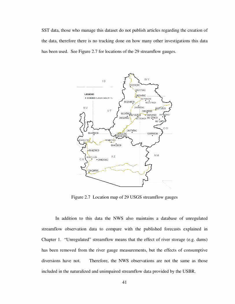
41
SST data, those who manage this dataset do not publish articles regarding the creation of
the data, therefore there is no tracking done on how many other investigations this data
has been used. See Figure 2.7 for locations of the 29 streamflow gauges.
Figure 2.7 Location map of 29 USGS streamflow gauges
In addition to this data the NWS also maintains a database of unregulated
streamflow observation data to compare with the published forecasts explained in
Chapter 1. “Unregulated” streamflow means that the effect of river storage (e.g. dams)
has been removed from the river gauge measurements, but the effects of consumptive
diversions have not. Therefore, the NWS observations are not the same as those
included in the naturalized and unimpaired streamflow data provided by the USBR.

42
The online database of unregulated forecasts and observations can be downloaded
from (http://www.nwrfc.noaa.gov/westernwater/?page=data&id=). The data include the
April – July forecasts generated January through July of each year, but not the yearly
outlooks generated in August and October. Therefore the “outlook” data will need to be
obtained from the CBRFC at a future time, after sufficient progress has been made. Also,
CBRFC references gauge identifications which are different from the USGS gauge ID
numbers used in the USBR streamflow data. However, from the description of the NWS
and USBR gauges a total of 18 gauges were identified to common between the two
datasets.
The proposed work will use only the forecast data obtained for these 18 gauge
locations to compare the results from the proposed research with the seasonal forecasts
generated by the NWS. It should be pointed out that for reasons similar to those with the
USBR streamflow data, the number of studies using this data is unknown.
2.7 Summary of Data
In total there are nine (9) data sets used in the proposed work:
• NCEP/NCAR Reanalysis Datasets 1948 through present:
o 500mb Geopotential Height
o 200mb Zonal Wind Data
• Southern Oscillation Index (SOI) – 1951 through present
• Pacific Decadal Oscillation (PDO) – 1900 through present
• Northern Atlantic Oscillation (NAO) – 1950 through present
• Atlantic Multidecadal Oscillation (AMO) – 1948 through present
• Extended reconstructed sea surface temperatures (ERSST v.3): 1854 - present
43
• USBR Naturalized/Unimpaired Streamflow: 1905 – Present for 29 locations
Because of the common length of records of the existing climate indices, the tasks
related to the first question will involve data from 1951 – 2004, and compare this with
observed yearly streamflow volumes from 1952 – 2005. Extended SVD analysis uses
streamflow data from 1952 – 2005 to compare with SST data from 1952 – 2005 (0-year
lag), 1952 – 2004 (1-year lag), 1951 – 2003 (2-year lag), and 1950 – 2002 (3-year lag)
SST gridded data. The associated correlation analysis in Chapter 4 uses the gridded
ocean data for similar lag times. Finally, and because the ESP is calibrated on the period
from 1976 – 2005, Chapter 5 will utilize the streamflow data from 1906 – 2005 to
complete the three different split sample analyses. This analysis will also require SST
data from 1904 – 2005.
44
CHAPTER 3
A BASIS FOR IMPROVING STREAMFLOW FORECASTING OF THE COLORADO
RIVER BASIN
3.1 Introduction
Recent research has provided many tools for the climate scientist to understand
the connection between sea surface temperatures (SSTs) and sea level pressure (SLP)
with surface climate over the United States (Latif and Barnett 1994; Hidalgo and Dracup
2003; McCabe and Dettinger 1999). Due to the recent drought conditions in the desert
southwest, much of this research focuses on ways to describe the streamflow of the
Colorado River basin, by observing large-scale climate observations over the Pacific
Oceans (Grantz et al. 2005; Kim et al. 2006; Kim et al. 2007). The well known
relationships between SST/SLP data and streamflow of the western United States are a
result of the El Niño Southern Oscillation (ENSO). However, there are many limitations
to what information the ENSO can provide water managers of the Colorado River Basin
(CRB) (McCabe and Dettinger 2002).
The first limitation is that the effects of the ENSO are most easily correlated with
surface climate of the northwestern and southwestern areas of the United States. There is
a large area covering central California, Nevada, Utah, Colorado and Wyoming which
does not respond consistently to ENSO variability. The supposition is at times this
region is influenced by northerly atmospheric conditions, and at other times southerly
conditions influence the region. Another limitation to the ENSO is that its effect on
surface hydrology of the western U.S. has a relatively short lead time. For instance,
McCabe and Dettinger (2002) found that fall-winter ENSO observations were correlated
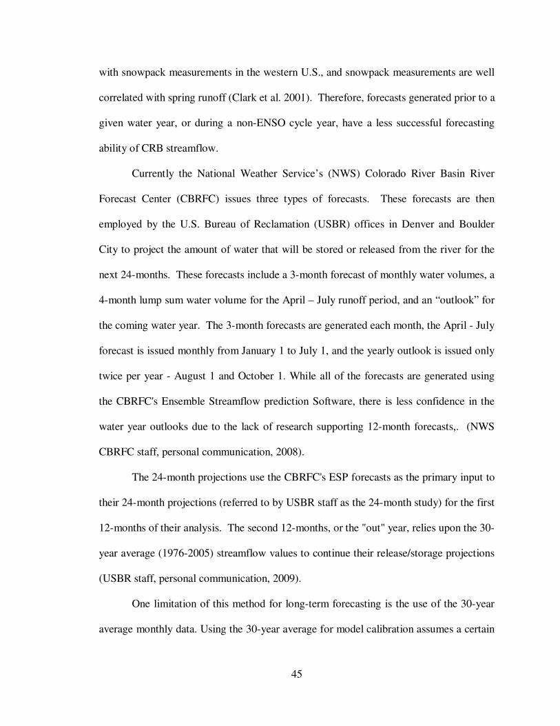
45
with snowpack measurements in the western U.S., and snowpack measurements are well
correlated with spring runoff (Clark et al. 2001). Therefore, forecasts generated prior to a
given water year, or during a non-ENSO cycle year, have a less successful forecasting
ability of CRB streamflow.
Currently the National Weather Service’s (NWS) Colorado River Basin River
Forecast Center (CBRFC) issues three types of forecasts. These forecasts are then
employed by the U.S. Bureau of Reclamation (USBR) offices in Denver and Boulder
City to project the amount of water that will be stored or released from the river for the
next 24-months. These forecasts include a 3-month forecast of monthly water volumes, a
4-month lump sum water volume for the April – July runoff period, and an “outlook” for
the coming water year. The 3-month forecasts are generated each month, the April - July
forecast is issued monthly from January 1 to July 1, and the yearly outlook is issued only
twice per year - August 1 and October 1. While all of the forecasts are generated using
the CBRFC's Ensemble Streamflow prediction Software, there is less confidence in the
water year outlooks due to the lack of research supporting 12-month forecasts,. (NWS
CBRFC staff, personal communication, 2008).
The 24-month projections use the CBRFC's ESP forecasts as the primary input to
their 24-month projections (referred to by USBR staff as the 24-month study) for the first
12-months of their analysis. The second 12-months, or the "out" year, relies upon the 30-
year average (1976-2005) streamflow values to continue their release/storage projections
(USBR staff, personal communication, 2009).
One limitation of this method for long-term forecasting is the use of the 30-year
average monthly data. Using the 30-year average for model calibration assumes a certain

46
amount of climate stationarity, a concept which lately has been challenged in light of
global climate trends (Milly et al. 2008). Another limitation of this method is that the
NWS/NRCS forecast, as well as the 24-month study, are deterministic forecasts. From a
practical standpoint, this means that the actual probability of each is not reported
therefore the quality of the forecast remains unknown. A final limitation is that the
forecasts created by the ESP view each of the historical inputs as equally likely in the
current forecast.
This Chapter proposes that one improvement to generating long-term forecasts
can be found by weighing the historical input data used by the ESP. Currently, after the
ESP generates its forecast traces for the forecast period, certain years can be assigned
more significance than others based on how similar the forecast year is to the calibrated
years. For example, if an El Niño event is taking place during the water year, El Niño
years from the historical record can be assigned more weight (e.g., Tootle e al., 2009).
While this post-analysis weighting is sometimes performed, this information is not used
to generate the official ESP forecast (CBRFC, Personal Communication, 2009).
However, developing a forecasting approach where the streamflow traces are weighted
post-analysis, provides a greater promise for implementation since the CBRFC are
already acquainted with the method. The key to finding an objective weighting measure
is to identify a long-lead climate indicator which provides a better indication to changes
in streamflow than the 30-year mean. The principle goal of this Chapter is to establish a
long-lead teleconnection between existing climate indices, or Pacific Ocean SST’s, and
CRB streamflow. A physical description of a long-lead teleconnection is the subject of
Chapter 4, which will be based on the results from the current chapter.

47
Much has been discovered about the connection of observed climate indices with
the current water year, or two season lag time between the climate and runoff
measurements (Grantz et al. 2005). This Chapter builds upon recent studies showing the
correlation of large scale climate index phases and streamflow or snowpack
measurements in the Colorado River Basin (Tootle et al. 2005; Clark et al. 2001; Werner
et al. 2004). Where this study differs from existing work (Timilsena et al, 2007) is that
measured data will be used to ascertain the effect of large scale climate on
unimpaired/naturalized CRB streamflow data, as opposed to using tree-ring reconstructed
streamflow data sets. Another departure from existing research (e.g. Werner et al 2004)
is that we will be analyzing the correlation of lead climate indices and the following
water year's volume over multiple lag times.
3.2 Data
There are a total of six (6) data sets used in this analysis: naturalized streamflow,
observed monthly Southern Oscillation Index (SOI), monthly Pacific Decadal Oscillation
(PDO) index, monthly Northern Atlantic Oscillation (NAO) index, monthly Atlantic
Multidecadal Oscillation (AMO) index, and Sea Surface Temperatures.
3.2.1 Naturalized Streamflow
The United States Bureau of Reclamation (USBR) maintains a database of
naturalized or unimpaired runoff data for the Colorado River Basin (CRB) and is
available for download from the following URL (http://www.usbr.gov/lc/region/
g4000/NaturalFlow/current.html). Streamflow gauges are considered naturalized when
the effects of human interference (e.g. dams and diversions) have been removed
(mathematically) from the gauge measurements. For the readers reference, there are two

48
other kinds of gauges data: Unimpaired and Impaired. Unimpaired gauges are those
which, for all intents and purposes, measure the natural flowrate of the river. Impaired
gauges measure streamflow which are affected by upstream storage or diversions. In all,
there are 29 streamflow gauges within the upper and lower CRB which report naturalized
streamflow from 1905 water year (October 1905 – September 1906) thru the 2004 water
year. This particular dataset is chosen for this analysis because the USBR uses this data
as input into their 24-month study, as well as the fact that it is referenced as the baseline
for all forecasts of the CRB. For example, a given CBRFC seasonal forecast is often
reported as a percentage of the 30-year average (1971-2000) streamflow volume using
this data). Figure 3.1 shows a map of the 29 river gauge locations.
3.2.2 SST and Climate Index Data
Average monthly SST values were obtained from the National Climatic Data
Center (http://www.cdc.noaa.gov/cdc/data.noaa.ersst.html). The data is presented in 2º x
2º grid cell for all oceans (Smith and Reynolds, 2003; Smith et al., 2008) and spans the
years from 1846 until present. Though the dataset is a reconstruction of SST values for
the period, data quality improves from 1950 on as a result of increase coverage ocean
monitoring capability. The range of ocean data used in this study covers the area from
Longitudes 120º East to 80º West and Latitudes 20º South to 60º North, which is similar
to the region studied by Tootle et al. (2006).
Climate index data can be found through the National Oceanic Atmospheric
Administration’s (NOAA) Climate Prediction Center (CPC) website. These indices have
been used previously to demonstrate a correlation between the changes in the index and
surface climate changes (Tootle et al. 2005; Shabbar et al. 1997; Rasmussen & Wallace,
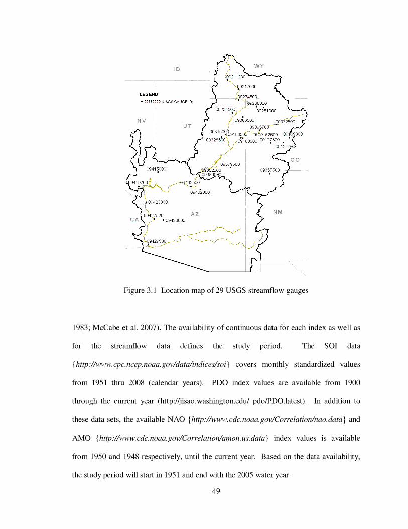
49
Figure 3.1 Location map of 29 USGS streamflow gauges
1983; McCabe et al. 2007). The availability of continuous data for each index as well as
for the streamflow data defines the study period. The SOI data
{http://www.cpc.ncep.noaa.gov/data/indices/soi} covers monthly standardized values
from 1951 thru 2008 (calendar years). PDO index values are available from 1900
through the current year (http://jisao.washington.edu/ pdo/PDO.latest). In addition to
these data sets, the available NAO {http://www.cdc.noaa.gov/Correlation/nao.data} and
AMO {http://www.cdc.noaa.gov/Correlation/amon.us.data} index values is available
from 1950 and 1948 respectively, until the current year. Based on the data availability,
the study period will start in 1951 and end with the 2005 water year.

50
3.3 Methodology
The correlation between the climate variability and SST with the gauge
streamflow was completed using two statistical methods. The first test is the Rank Sum
Test. This test is used to compare mean values from two different datasets to determine
if they are significantly different. The second test is the Singular Value Decomposition
(SVD) method of finding maximum covariance between two fields. SVD was used to
compare the SST data with the streamflow data.
3.3.1 Rank Sum Analysis
The rank sum test is an excellent way to test a “before” and “after” scenario
without trying to determine if either data set has a defined distribution. Alternatively, it
can be used to test for differences between two segmented data sets. Hence, this is a non-
parametric test and does not make assumptions about the distributions of either dataset. In
the current analysis, we are using the negative and positive phases of the indices to act as
our “before” and “after conditions respectively. The mean of the streamflow measured
during a negative climate phase is compared with the mean streamflow measured during
the positive climate phase. The null hypothesis of this test is that the means from the two
sample sets are equal. The results of a rank sum test provide a value of the probability
that the two sets are similar. For p-values less than 0.05, the null hypothesis was rejected
a theoretical discussion of this test is offered by Alder and Roessler (1977).
In order to determine the effect that the SOI has on CRB streamflow the 3-month
and 6-month average SOI values were used to separate the historical streamflow data into
“positive” and “negative” groups. Figure 3.2 shows an overview of how the rank sum
test uses the historical index values to compare the positive and negative streamflow
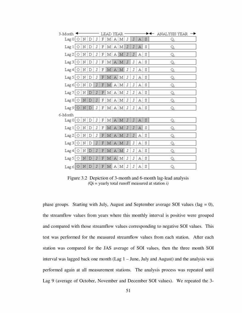
51
Figure 3.2 Depiction of 3-month and 6-month lag-lead analysis (Qi = yearly total runoff measured at station i)
phase groups. Starting with July, August and September average SOI values (lag = 0),
the streamflow values from years where this monthly interval is positive were grouped
and compared with those streamflow values corresponding to negative SOI values. This
test was performed for the measured streamflow values from each station. After each
station was compared for the JAS average of SOI values, then the three month SOI
interval was lagged back one month (Lag 1 – June, July and August) and the analysis was
performed again at all measurement stations. The analysis process was repeated until
Lag 9 (average of October, November and December SOI values). We repeated the 3-
52
month average rank sum test for the PDO (index No. 2), NAO (No. 3), and AMO (No. 4)
indices, which provided a total of 1,160 results (29 stations x 10 lags x 4 indices).
Similarly we performed the same process for the 6-month average values starting with
the April-September interval (AMJJAS; lag = 0) and ending with the October-March
interval (ONDJFM; lag = 6) (see Figure 3.2). The 6-month analysis consisted of an
additional 812 rank sum tests (29 stations x 7 lags x 4 indices).
3.3.2 Combination of Indices
The next step in the analysis was to compare the combined effect of the indices
assuming that the influence from different climatic phenomena can occur at the same
time. The process used to determine the effect of an individual climate index was
repeated for the combination analysis. This process is shown graphically in Figure 3.3.
Using the SOI as a base, the combination analysis compared the PDO-positive and PDO-
negative values which also occur under an SOI-positive phase (Labeled as analysis No.
5). Likewise, the process was repeated for PDO-positive vs. PDO-negative values under
the SOI-negative phase (analysis No. 8). The SOI-PDO combination of 3-month and 6-
month average values included an additional 986 rank sum tests (29 stations x 10 lags x 2
combination phases + 29 x 7 x 2). In a similar manner, the NAO (analysis No. 6 & 9)
and AMO values (analysis No. 7 & 10), were also completed for the 3- month and 6-
month values. Therefore the combination analyses yielded a total of 2958 results (986 x
3 indices).

53
Figure 3.3 Combination rank sum testing using the SOI as a basin
3.3.3 SVD Analysis of Pacific Ocean SSTs
The next step in the analysis process was to determine how Pacific Ocean sea
surface temperatures vary with respect to the streamflow measured in the 29 gauges of
the CRB. The goal of this analysis was to determine if there is any SST pattern that can
be identified, which is not already represented in one of the indices used in the rank sum
testing. The process is also known as Maximum Covariance Analysis, because the goal
is to identify the dimensions, or modes, which represent the maximum amount of
covariance between two temporal fields. Since the spatial component of most climate
data is quite large, using the temporal field to compare generally limits the analysis
dimension to the number of days, months, or years included in the study period. In this
paper our time scale is in years.
The use of SVD to find couple patterns in climate data was explored by
Bretherton et al. (1992) who compared five different methods for analyzing climate data.
Other research (Wallace and Bretherton 1992; Soukup et al. 2010) has utilized SVD to
analyze the covariance of sea level pressure as well as SST with snow water equivalent
measurements, precipitation, and, as we do here, with streamflow. The process
performed in this analysis is similar to Tootle and Piechota (2006), where SST anomalies

54
in the Pacific Ocean are coupled with streamflow anomalies across the United States. In
this paper we limit the analysis to the CRB streamflow only.
The following description of the SVD process is provided by several sources
(Bretherton et al. 1992; Wallace et al. 1992). Before any computations were performed,
the raw SST and Streamflow data were standardized based upon each grid location and
the values representing land (values of -9999) were deleted from the SST matrix. Next, a
covariance matrix using the SST and Streamflow anomalies was determined using the
following formula:
COVARTS = (1/n) (T'S)
In this analysis, the number of years in the temporal analysis is, n = 53. The SST field
[53 x 3218] was represented by the letter, T, and S represents the streamflow data field
[29 x 53]. The SVD was performed on the COVARTS matrix [3218 x 29] which yielded
the following three matrices:
SVD(COVARTS) = U Σ V
U [3218 x k] and V [29 x k] represent the left and right singular (heterogeneous) matrices
respectively, and Σ [53 x 29] represents the diagonal matrix of singular values from the
SVD. The value k, represents all modes (columns in the matrix) which contain a squared
covariance fraction (SCF) > 10%. SVD (similar to the results from a PCA/EOF analysis)
attempts to describe the variance of a given matrix (in this case, the COVARTS matrix) by
drawing new axes which are rotated in matrix space to capture as much of the variance
(in essence, changes in SST or streamflow) as possible. Each column of the U and V
represents a new axis and the values in those columns represent the variance captured by
that axis. In order to measure the proportion of variance contained within a given

55
column, Bretherton et al. (1992), used the squared covariance fraction (SCF). The SCF is
found by dividing the square of each singular value in the Σ matrix by the sum of the
squared singular values (sum of squared values from the diagonal) as is shown by the
following equation:
2,
292,
1
i i
i i
i
SSCF
S=
=
∑
In this equation S represents the matrix of singular values Σ (substituted to avoid
confusion with the summation sign in the denominator), and the summation is taken for
values of i from 1 to 29 because this is the total number of columns of Σ.
Finally, the left and right temporal expansion series (LTES & RTES) were
obtained by projecting U onto T and V onto S in the following manner:
LTES = U’ T’
RTES = V’ S’
The LTES [53 x k] and RTES [53 x k] expansion series are both time series representing
the maximum yearly variance of the SST data. The LTES is then standardized to reflect
the unit increments of variance. In this format the LTES can now be used in the same
way that the climate indices were used to test correlation with the streamflow in the rank
sum test. The LTES is run through the lagged correlation testing outlined above, just like
the testing approach to the established climate indices.
The final step in the analysis was to determine the significance of the variance
observed in the left heterogeneous field (SST) and the right heterogeneous field
(streamflow), by calculating the Pearson-r correlation coefficient. The testing for
significance was done using a student t-test, which assumes that the correlation

56
coefficients are normally distributed with a mean value of r = 0. Working backwards,
starting with n – 2 degrees of freedom (i.e. 51), we find that |r| ≥ 0.27 in order to be
significant. This value is based on α = 0.05.
3.3.4 Forecast Skill Comparison
The final analysis proposed in this chapter is used to compare the forecast skill
abilities up to three climate indices at a time. In contrast to the Rank sum analysis, which
provides an assessment of significant dissimilarities between streamflow observed under
the positive and negative phases of a given index, the forecast skill score will calculate a
value which represents the magnitude of contribution that a given index makes to a given
forecast model. The comparison between the three indices was completed using a model
initially developed by Piechota et al (1998) who were trying to develop long lead-time
forecasts of streamflow in Eastern Australia. A detailed explanation of the method is
provided in Piechota et al (1998) and in other more recent research (Tootle and Piechota,
2004; Soukup et al, 2010). A brief explanation is provided here.
A probability density function is created using a kernel density estimator and a
sorted vector of observed streamflows at a given location. For each observed streamflow
a unique probability value is obtained using a given predictor (SOI, PDO, and so forth).
The streamflow/probability data pairs are then plotted to create a probability exceedance
curve for each predictor. The three exceedance curves are combined to create a
composite exceedance curve which is the basis for the forecast model. This new forecast
model calculates weights a, b, and c which are applied to the appropriate predictors to
optimize the forecast model’s linear error in probability space (LEPS) score. The LEPS
score was initially developed by Ward and Folland (1991) and subsequently revised by

57
Potts et al (1996). The revised LEPS score is used here since the formula proposed by
Potts et al. gives a higher score to forecasts of extreme values than to forecasts closer to
the observe mean.
3.4 Results
There is one limitation to the rank sum test and its significant results. In the
current analysis there are a total of 11 climate indices (four climate indices, six
combinations of the same, and the LTES) which yielded a total of 5,423 rank sum test
results. Of these tests there were a total of 828 significant test results. Based on the
chosen α for our analysis, 272 of the significant results (5,423 x 0.05) have a probability
of representing Type I errors. In other words, approximately 1/3 of the significant results
can come back as false positives. To address this issue, the total number of successful
results at each streamflow gauge station was ranked according to the p-value resulting
from the Rank Sum test. P-values close to 0.05 have the highest chance of a Type I error,
so only the two lowest p-values at each station were reported.
3.4.1 Climate Indices
Figure 3.4 shows the total number of successful results from each climate input.
By far, the most successful index input to the rank sum test is the LTES. In fact, the Jan-
Feb-Mar LTES rank sum test resulted in significant results at all 29 stations. It is also
interesting to point out that the next largest number of successful results came from the
NAO and the AMO index tests. As the analysis lag increased so did the number of
successful results attributed to the AMO. Table 3.1 shows the top two index inputs at
each gauge location. The SST index references in Figure 3.4 is the LTES resulting from
the SST-Streamflow SVD analysis for the given interval length and lag number.
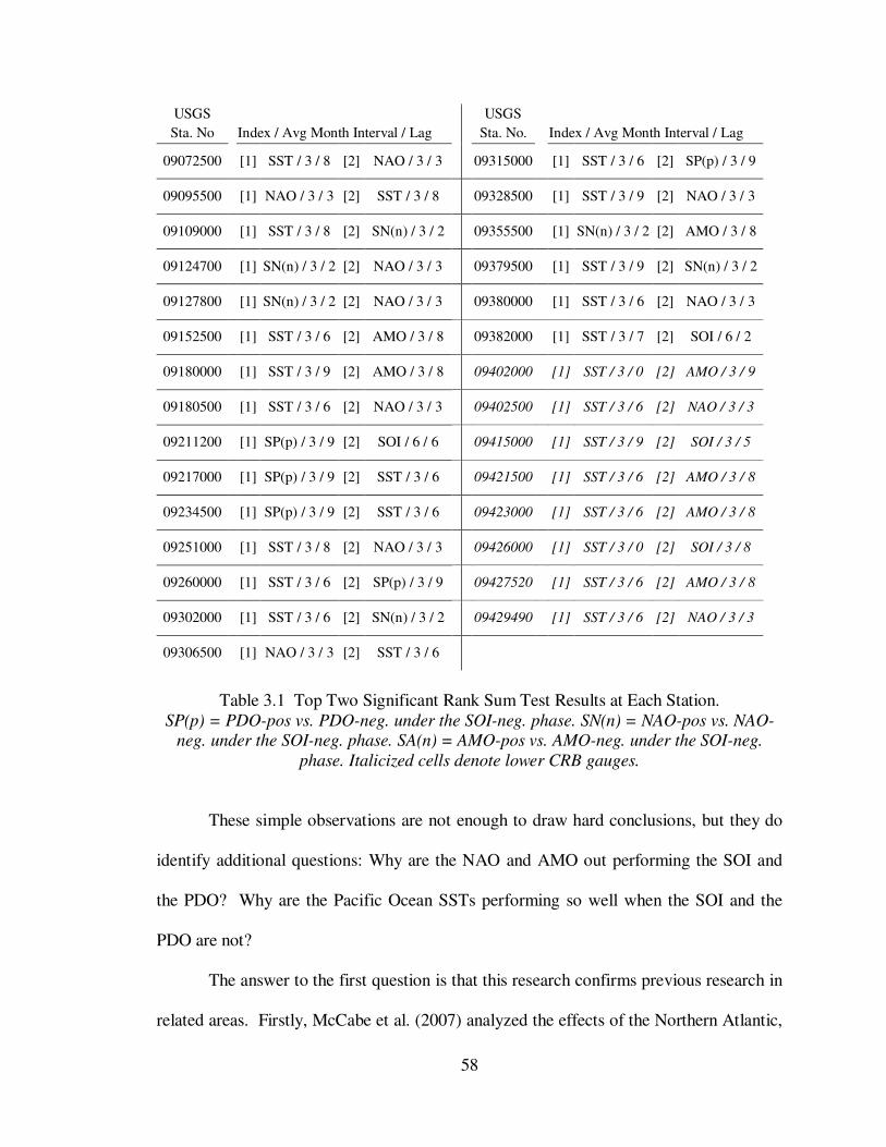
58
USGS Sta. No
Index / Avg Month Interval / Lag
USGS Sta. No.
Index / Avg Month Interval / Lag
09072500 [1] SST / 3 / 8 [2] NAO / 3 / 3 09315000 [1] SST / 3 / 6 [2] SP(p) / 3 / 9
09095500 [1] NAO / 3 / 3 [2] SST / 3 / 8 09328500 [1] SST / 3 / 9 [2] NAO / 3 / 3
09109000 [1] SST / 3 / 8 [2] SN(n) / 3 / 2 09355500 [1] SN(n) / 3 / 2 [2] AMO / 3 / 8
09124700 [1] SN(n) / 3 / 2 [2] NAO / 3 / 3 09379500 [1] SST / 3 / 9 [2] SN(n) / 3 / 2
09127800 [1] SN(n) / 3 / 2 [2] NAO / 3 / 3 09380000 [1] SST / 3 / 6 [2] NAO / 3 / 3
09152500 [1] SST / 3 / 6 [2] AMO / 3 / 8 09382000 [1] SST / 3 / 7 [2] SOI / 6 / 2
09180000 [1] SST / 3 / 9 [2] AMO / 3 / 8 09402000
[1] SST / 3 / 0 [2] AMO / 3 / 9
09180500 [1] SST / 3 / 6 [2] NAO / 3 / 3 09402500
[1] SST / 3 / 6 [2] NAO / 3 / 3
09211200 [1] SP(p) / 3 / 9 [2] SOI / 6 / 6 09415000
[1] SST / 3 / 9 [2] SOI / 3 / 5
09217000 [1] SP(p) / 3 / 9 [2] SST / 3 / 6 09421500
[1] SST / 3 / 6 [2] AMO / 3 / 8
09234500 [1] SP(p) / 3 / 9 [2] SST / 3 / 6 09423000
[1] SST / 3 / 6 [2] AMO / 3 / 8
09251000 [1] SST / 3 / 8 [2] NAO / 3 / 3 09426000
[1] SST / 3 / 0 [2] SOI / 3 / 8
09260000 [1] SST / 3 / 6 [2] SP(p) / 3 / 9 09427520
[1] SST / 3 / 6 [2] AMO / 3 / 8
09302000 [1] SST / 3 / 6 [2] SN(n) / 3 / 2 09429490
[1] SST / 3 / 6 [2] NAO / 3 / 3
09306500 [1] NAO / 3 / 3 [2] SST / 3 / 6
Table 3.1 Top Two Significant Rank Sum Test Results at Each Station.
SP(p) = PDO-pos vs. PDO-neg. under the SOI-neg. phase. SN(n) = NAO-pos vs. NAO-
neg. under the SOI-neg. phase. SA(n) = AMO-pos vs. AMO-neg. under the SOI-neg.
phase. Italicized cells denote lower CRB gauges.
These simple observations are not enough to draw hard conclusions, but they do
identify additional questions: Why are the NAO and AMO out performing the SOI and
the PDO? Why are the Pacific Ocean SSTs performing so well when the SOI and the
PDO are not?
The answer to the first question is that this research confirms previous research in
related areas. Firstly, McCabe et al. (2007) analyzed the effects of the Northern Atlantic,
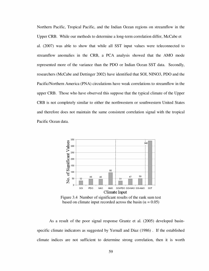
59
Northern Pacific, Tropical Pacific, and the Indian Ocean regions on streamflow in the
Upper CRB. While our methods to determine a long-term correlation differ, McCabe et
al. (2007) was able to show that while all SST input values were teleconnected to
streamflow anomalies in the CRB, a PCA analysis showed that the AMO mode
represented more of the variance than the PDO or Indian Ocean SST data. Secondly,
researchers (McCabe and Dettinger 2002) have identified that SOI, NINO3, PDO and the
Pacific/Northern America (PNA) circulations have weak correlations to streamflow in the
upper CRB. Those who have observed this suppose that the typical climate of the Upper
CRB is not completely similar to either the northwestern or southwestern United States
and therefore does not maintain the same consistent correlation signal with the tropical
Pacific Ocean data.
Figure 3.4 Number of significant results of the rank sum test based on climate input recorded across the basin (α = 0.05)
As a result of the poor signal response Grantz et al. (2005) developed basin-
specific climate indicators as suggested by Yernall and Diaz (1986) . If the established
climate indices are not sufficient to determine strong correlation, then it is worth

60
evaluating whether other regions of the Pacific may serve as predictors. It is along this
line of reasoning that the second question was explored: why does the temporal
expansion series from the SVD analysis outperform the established climate indices?
3.4.2 Pacific Ocean SSTs
The SVD analysis provides a number of maps which provide a helpful amount of
information about what might be a basin-specific climate index (See Figures 3.5 and 3.6).
These figures are generated by plotting the significant correlation coefficients of the left
(SST) and right (streamflow) heterogeneous matrices. Starting at lag = 0 (Jul-Aug-Sep &
Apr-May-Jun-Jul-Aug-Sep) there is a visible signal from the ENSO region of the Pacific
which diminishes as the lag number increases. Conversely, as the lag number increases,
another area located east and south of Japan begins to grow until reaching its maximum
size around lag = 6 for the 3-month average interval, and lag = 4 for the 6-month
interval). The difference in sign between the ocean area east of Japan and the streamflow
gauges shows that they are negatively correlated: as one is increasing, the other is
decreasing.
It is interesting to observe that the region in question is anchored over an area that
this paper defines as 150 E to 200 E (160 W) and from 24 N to 34 N. This particular area
is south and west of the area which is associated with the northern Pacific signals of the
PDO as identified by Mantua and Hare (2002). However, this area is not original to the
current research as it has been identified in other research without being specifically
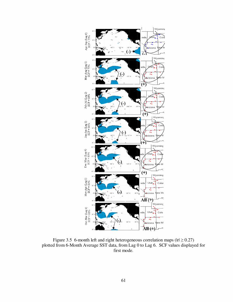
61
Figure 3.5 6-month left and right heterogeneous correlation maps (|r| ≥ 0.27) plotted from 6-Month Average SST data, from Lag 0 to Lag 6. SCF values displayed for
first mode.
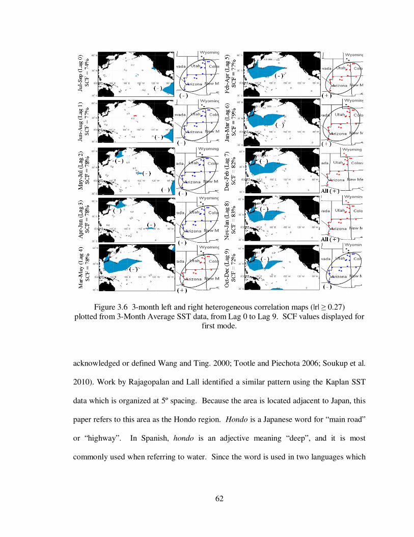
62
Figure 3.6 3-month left and right heterogeneous correlation maps (|r| ≥ 0.27) plotted from 3-Month Average SST data, from Lag 0 to Lag 9. SCF values displayed for
first mode.
acknowledged or defined Wang and Ting. 2000; Tootle and Piechota 2006; Soukup et al.
2010). Work by Rajagopalan and Lall identified a similar pattern using the Kaplan SST
data which is organized at 5º spacing. Because the area is located adjacent to Japan, this
paper refers to this area as the Hondo region. Hondo is a Japanese word for “main road”
or “highway”. In Spanish, hondo is an adjective meaning “deep”, and it is most
commonly used when referring to water. Since the word is used in two languages which

63
are geographically relevant to the research at hand and its meanings are relevant to the
research, this region of the ocean lends itself to this designation.
The success of the LTES as an index can be explained through the way in which it
is created and how it can be used. Since the LTES is the projection of the SST variance
onto the normalized raw SST data, the result is a vector which represents the scaled SST
variance within the given 3-month (or 6-month) interval of time selected for the analysis.
For all but three of the analysis periods (3-month, lags 0 and 1, as well as 6-month lag 0),
the overwhelming majority of the variance could be explained by the first mode, and is
therefore captured as part of the LTES. We hypothesize that this is because the influence
of other climate indices is stronger during these periods than the rest of the year. The
LTES may seem less ideal to use because it is not simply the standardized SST values of
the Hondo region (similar to the PDO, or AMO). As already shown the LTES is the
product of the SST and Streamflow data. Which creates another question: How do you
create a forecast with a model that requires the forecast point in order to be created? We
do not propose to answer this question here. However, since the Hondo region is
identified by an SVD analysis it is best to continue discussing the SST-streamflow
connection in terms of the SVD output (in essence, the left temporal expansion series).
The teleconnection between the SSTs of the western pacific and the streamflow
may be explained from the perspective of the East Asian Jet Stream (EAJS). Zhang et al.
(1997a) demonstrated that the presence of high pressures over Siberia, and cold surges
from east Asia (travelling on a south-southeast direction from northern china), have a
great effect on the winter monsoon season over East Asia. A strong East Asia winter
monsoon is characterized by two high-pressure centers: the first is a warm high pressure
64
center whose mid-point is roughly east of Papua New Guinea while the other center is a
cold “dome adjacent to the Siberian region”. Between the two high pressure centers is
the winter traveling path of the East Asian Jet Stream.
Athanasiadis et al (2010), show that the Hondo region is actually the terminus of
the EAJS (Asian/Pacific Jet). By completing an EOF (i.e. PCA) of the average
wintertime (Dec-Mar) wind field over the northern hemisphere, this study identified the
path of the dominant Asian/Pacific jet. Figure 4 of Athanasiadis et al. (2010) is of special
note because it displays the dominant wintertime jet (shown in a heavy black line) based
on the EOF analysis superimposed upon the teleconnectivity of the 250hPa zonal wind
and the 500hPa geopotential height fields (Wallace and Gutzler, 1981, define
teleconnectivity as the absolute value of the strongest negative correlation between a grid
point and any other grid point). This figure shows that the terminus of the Asian/Pacific
Jet is approximately 150 W, and between 30 N and 35 N. This coincides fairly well with
the eastern boundary of the Hondo Region. Athanasiadis et al continue to show that while
the first mode of the Asian/Pacific jet EOF is closely correlated with the Pacific/North
American (PNA) index, the second mode is not identified as being tied to a specific
index. However, it is the second mode which determines the location of the
Asian/Pacific Jet (and therefore the EAJS) and the storm track that encroaches on the
west coast of North America. It is the second mode of the teleconnectivity patterns
which approximate the location of the Hondo region the best.
Yang et al. (2002) identified the consistency at which the EAJS crosses the
southern Japanese island of Kyūshū and enters the Hondo region. Yang et al. further
identified that as the position of the EAJS changes, there are corresponding changes in
65
SSTs over the eastern Pacific Ocean and western North America. During the strong
winter monsoon events, Zhang et al. (1997a) showed that the surface wind patterns show
that the EAJS “bifurcates” shortly after exiting the Hondo region. A portion of the flow
pattern turns southeast and enters the path of the jet stream. The other portion is diverted
north and joins the Aleutian low. Both air streams ultimately cross into the western
United States thereafter.
We hypothesize that the EAJS is the vehicle by which strong Monsoonal moisture
is carried from East Asia to western North America. Incidentally, Sun and Sun (as cited
in Zhang et al. 1997b) propose that a strong winter monsoon usually precedes a drought
summer season in East Asia. We hypothesize that operating in such conditions, moisture,
which normally would remain in East Asia is carried by the bifurcated wind flow toward
North America. The northerly flow path carries some of the moisture to the western
United States where it is deposited as snowfall within the CRB (Aziz et al., 2010).
3.4.3 Forecast Skill Comparison Results
After the SVD and Rank Sum testing is complete, a Hondo index is defined as the
LTES of the SVD analysis and then compared to the SOI and PDO index. While the use
of indices (e.g., SOI, PDO) may result in skillful long lead-time forecasts of streamflow,
some streamflow regions may not be teleconnected to established climate signals and,
thus, would result in less than skillful forecasts when using such indices. A distinct
advantage of applying SVD to SST and streamflow regions is the possible identification
of a new SST region that, when used in a forecast model, results in a skillful streamflow
forecast.

66
The Forecast Skill Comparison method described earlier was employed using the
SOI, the PDO, and the SST LTES (taken from the JFM SVD analysis) as the third
predictor. Figure 3.7 displays the results from this analysis. At this lag time, the analysis
shows that the SOI and the PDO result in negative forecast skill values (i.e. their
forecasts are less accurate than the observed mean). On the other hand the SST LTES
provided an improvement to the forecast skill over the observed mean demonstrating the
potential for the new region of the ocean to be used as a forecasting tool.
Figure 3.7 Plots showing contribution of index to forecast skill.
Value of ‘0’ is a forecast as good as the mean.
67
3.5 Conclusion
The goal of this analysis was to find which climate data, combination of climate
data, and lead time could be used to increase the skill of forecasting streamflow on the
first day of the following water year. The rank sum testing from this research identified at
least two different climate inputs for every river gauge in the CRB. For each of the 29
river gauges, there was a significant correlation with an established climate index.
However, when comparing the number of successful tests from the different climate
inputs, the SST data was more consistent at providing significant results.
Further testing using SVD showed that a long-term correlation exists between the
SST anomalies and streamflow anomalies for the Colorado River Basin. SVD testing of
3-month averaged SST data, showed that a region bounded by 150 E to 160 W and 24 N
to 34 N, named here as the Hondo region, demonstrates a significant amount of
covariance with the streamflow measured over the following water year. As already
mentioned, the significance of this region has been demonstrated in other research. The
success of the Hondo region lays in the strength and consistency of the Asian winter
monsoon, and the effectiveness of the East Asian Jet Stream to transport the moisture
across the Pacific Ocean.
The results obtained in this research demonstrate the potential to generate long-
lead forecasts of CRB streamflow from SST values observed over the Hondo region in
the Pacific Ocean. Therefore, the next steps include identifying a forecast approach
which utilizes the climate CRB-streamflow connection observed here. The new work
should include a variety of input alternatives to determine the simplest and most effective
forecasting model for the entire water year, or simply the seasonal runoff (April – July).

68
CHAPTER 4
CONNECTING THE PACIFIC OCEAN TO THE COLORADO RIVER BASIN
4.0 Introduction
In recent years there has been increased interest to identify climate-hydrology
response relationships using the gridded global data such as sea surface temperature
(SST), pressure or zonal wind field data rather than looking to the established climate
indices, defined by a subset of the global data, such as the El Niño Southern Oscillation
(ENSO) or the Pacific Decadal Oscillation (PDO). The typical application of the global
gridded data is to identify covariance relationships between regions of the oceans and
surface hydrology such as precipitation, snowpack, and streamflow (Wang and Ting,
2000; Serrano and Rodriguez, 2004; Tootle et al., 2006; Haylock, 2007; Santos et al.,
2007; Yuan and Li, 2008; Apipattanavis et al., 2009; Soukup et al., 2010; Wu et al., 2009,
Wang et al., 2010a).
The research presented here builds upon Lamb et al (2010) and Aziz et al. (2009)
(hereafter referred to as L10 and A10 respectively) which shows there is an area of the
Pacific Ocean (150E - 200E, 34N - 24N – hereafter referred to as Hondo) which
demonstrates a significant correlation with streamflow in the Colorado River Basin
(CRB). Both (L10) and (A10) identified this region using a singular value decomposition
(SVD) analysis approach. In both cases the Hondo region was identified by isolating the
areas whose correlation coefficients exceeded a 95% significance level. Results in (L10)
reveal the Hondo region as significant when comparing the winter time SST’s from a
given water year, with the total yearly streamflow of the following water year. Similarly
(A10) identifies the Hondo region when correlating Pacific SSTs with snow water
69
equivalent (SWE) data from SNOTEL stations located throughout the U.S. Rocky
Mountains, also at a year’s lag time.
The existing research has left several questions to be answered regarding the
Hondo-CRB teleconnection. For example, because the studies L10 & A10 only looked at
comparing SST with the streamflow/SWE for the following water year, there is a need to
understand how persistent the Hondo effects are noticed in the CRB. In other words, do
the Hondo effects appear when climate data are compared with streamflow responses
from the same water year, as well as at lead times of more than one water year?
Additionally, since SST’s and streamflow are independent variables and are far apart,
what is the mechanism connecting the two?
The proposed research has two major tasks: First, the SVD analysis performed in
previous papers (L10 & A10) will be extended to include 4 years of SVD analysis:
simultaneous response year, and the three years leading up to it. This extended SVD
analysis is expected to identify the extent to which the Hondo effects the CRB. Second,
the SVD analysis will be applied to atmospheric datasets (such as geopotential height
(500mb) and zonal wind (200mb) to delineate dynamical responses to the SST-
streamflow relationship identified in the SVD analysis. The hypothesis is that if there is a
long-lead physical connection between the Hondo and the CRB streamflow, then the
Hondo-CRB teleconnection will appear in the other atmospheric datasets at similar lag
times. The goal of this work is to improve the understanding of the climate drivers for the
CRB in order to develop an improved long-lead forecasting technique.
70
4.1 Data
4.1.1 Streamflow Data
The US Bureau of Reclamation (USBR) maintains a spreadsheet of naturalized
streamflow data for 29 gauges within the CRB which can be obtained from the following
URL (http://www.usbr.gov/lc/region/g4000/NaturalFlow/current.html). Since a given
water year actually begins and ends in different calendar years, when this report refers to
a given water year (for example, 1996) it is signifies the period October 1, 1995 through
September 30, 1996. Therefore when the total yearly streamflow of a given water year is
shown, this is referring to the total water volume observed at a given gauge from October
1 through September 30 of the specified water year. In order to maintain some continuity
between the previous and current work, this data set is used here because it was used in
(L10). The 29 locations are displayed in Figure 4.1.
The SST data comes from work provided by Smith et al (2008) and can be
downloaded from the National Oceanic and Atmospheric Administration (NOAA)
National Climate Data Center (NCDC) website (http://www.ncdc.noaa.gov/oa/climate/
research/sst/ersstv3.php). The SST data are displayed at a 2˚ square grid spacing, and
were converted into text files using software, named Ocean Temperature Analysis
(OTA), developed at UNLV specifically for this purpose. Apart from the works of Aziz
et al., and Lamb et al. this particular SST data has been used in previous works to identify
a connection between ocean activity and the response in western U.S. streamflow (Tootle
and Piechota, 2006; Tootle et al, 2007; Soukup et al. 2010).

71
Figure 4.1 Location map of 29 USGS streamflow gauges
4.1.2 Climate Data
The 500mb geopotential height (Z500) and 200mb zonal wind field (U200), are
obtained from the NCEP/NCAR reanalysis product (Kalnay et al, 1996) available for
download at http://www.esrl.noaa.gov/psd/. The data for the variables listed covers the
entire globe at 2.5º square grid spacing. For this analysis, only the northern Pacific
Ocean region will be used, (in essence, 120E – 80W and 70 N to the equator (0). Since its
inception the reanalysis product has been used in thousands of applications to provide a
better understanding of global circulation patterns (Roundy and Gribble-Verhagen 2010;
Roundy et al. 2010; Pauluis et al. 2010; Grise et al. 2010), or to improve the

72
understanding of the connection between global climate and associated responses in
hydrologic phenomena (Wang et al., 2010a; Johnstone 2010; Johnstone 2010; Zhao et al.
2009; Patricola and Cook 2009; Fu et al, 2009; Adam et al, 2009) More relevant to the
current research, there are some recent examples of how this data is used to improve the
understanding of climate impacts on the CRB and closely related areas. Lundquist and
Flint (2006) used the data in order to identify reason for the early snowmelt-streamflow
runoff season in the Sierra Nevada Mountains observed in 2004. A study by Gochis et al.
(2007) looked at the North American Monsoon and its lagged correlation relationship
with Pacific and Caribbean Ocean SSTs. Bracken et al (2010) utilized the global dataset
to identify potential predictors of streamflow within the CRB. The studies not only
demonstrate the applicability of this data, but the utility of using these data as opposed to
another dataset.
4.2 Methodology
In (L10), the SVD analysis was performed using 3-month average SST values
from July – September and the observed streamflow volume generated during the
following water year (October 1 – September 30). This analysis was repeated for June –
August average SST values (Lag = 1 Month), for May – July (Lag = 2 Months), and so
forth until the average SST values from October – December (Lag = 9 Months) was
compared with the water volume from following water year.
In the research presented here the analysis includes comparing SST values and
streamflow values with a 0-year lag (simultaneous response year), as well as at 1-, 2- and
3-year lag times, essentially reproducing some of the work provided in Lamb et al (2010),
but adding additional lag times. Figure 4.2 demonstrates the progression of the lagged

73
SVD analysis. However, due to the large number of correlation maps, only the July –
September (JAS), April – June (AMJ), January – March (JFM), and October – December
(OND) intervals will be displayed here.
Figure 4.2 Lagged analysis schematic
The SVD analysis itself has been used in many applications when comparing the
behavior of two datasets (Prohaska, 1976; Bretherton et al. 1992; Wallace et al. 1992).
The method is described in detail in (L10). The purpose of the method is to identify
locations in the ocean and streamflow data that are significantly correlated to the
principle components identified in the SVD analysis. If the squared covariance fraction
(i.e. the percentage of variance explained by a given mode) of the principle component is
greater than 10%, then it is used in the correlation analysis. A 95% confidence level is
set to determine if the calculated correlation value is occurring by chance. Because the
CRB is a relatively small area, it is expected that the vast majority of the variance will be
explained by the first mode of the SVD analysis.
The purpose of this analysis is to identify the extent of the impact the Hondo has
on the CRB streamflow. It is expected that this analysis will show the Hondo as non-
significant in the 0-year lag because of the noise created by extreme ENSO cycles. It is

74
also expected that the strongest connection will be with the one-year lag, and then a
diminishing connection as the lagged analysis increases into the second and third years.
In addition to providing an extended SST-Streamflow SVD analysis (SST-SVD),
the current research proposes to utilize the extended SVD results to identify the
correlation with Z500 and U200 datasets. These correlation analyses use the streamflow
temporal expansion series that is calculated as part of the SVD analysis. While a detailed
description of this calculation is provided in L10, a brief explanation of how the temporal
expansion series is determined is provided here. The SVD on the SST – Streamflow
covariance matrix gives three matrices [SVD(covarTS) = U Σ V], where V represents the
decomposed covariance values closely associated with the streamflow. Therefore, given
the decomposed matrix, V, and the original matrix of streamflow anomalies, S, the
streamflow temporal expansion series (STES) is determined by the following equation:
STES = V’S’. The result of this calculation is a series of values, one for each time period
in V and S. The STES is then correlated with cell of the Z500 and U200 gridded data so
that the correlation responses portray possible circulation anomalies linking SSTs to CRB
streamflow.
4.3 Analysis Results
4.3.1 Extended SVD Results
Extended SVD analysis results are displayed in Figures 4.3 and 4.4. Figures 4.3(a) and
(b) show the SST-SVD results from the simultaneous response year, and the 1-year lag
time respectively. Figures 4.4(a) and (b) show the results from the 2-year and 3-year lag

75
Figure 4.3 0-year and 1-year lag correlation maps from SVD analysis
Figure (a) shows the correlation maps (α = 0.05) for the simultaneous response year and (b) 1-year lag. Red SST regions/Streamflow gauges show increasing temperatures and streamflow, while blue shows decreasing temperatures and streamflow. The Hondo is
shown as dashed rectangle.

76
Figure 4.4 2-year and 3-year lag correlation maps from SVD analysis
Same as Figure 3, but showing the (a) 2-year lag and the (b) 3-year lag times.

77
times. The "SCF" values labeled on each map represent the squared covariance fraction
for the mapped, SVD analysis mode. A black dashed line shows the limits of the Hondo
Region as defined by L10 and A10.
These figures display regions of the Pacific Ocean that are linked to streamflow
gauges in the CRB. Red/Blue regions of the Pacific Ocean denote increasing/decreasing
temperature teleconnections. Similarly, up-oriented red triangles and down-oriented blue
triangles represent increasing or decreasing streamflow teleconnections respectively. If
the significant region of the ocean and a streamflow gauge have the same color, then this
denotes a positive correlation relationship. If the SST and streamflow regions have
opposite colors then this displays a negative correlation relationship. If the maps display
a region of cool SSTs correlated with increasing streamflow, then we can also say that
warm SSTs over the same region will be associated with decreasing streamflow gauges.
During the simultaneous response year analysis, one notices that depending on the
time of year, the Hondo or the Eastern Equatorial Pacific Ocean SSTs are more
significant. Figure 4.3b, 1st Year Lag analysis, and Figure 4.4a, 2nd Year Lag show how
the Hondo is again significant during the winter months, though during the 2nd year, it
appears that the impact of the Hondo is diminishing. By the 3rd lag year, the impact of
the Hondo is diminished and the central equatorial Pacific Ocean develops into a
significant SST region. It is noteworthy that as the lag increases, the Squared Covariance
Fraction (SCF) represented in the correlation maps also increases. It is hypothesized that
as the lag time increases there is less SST-CRB covariance contained in the data.
Therefore it is easier for the first mode to represent more of the data (increasing SCF
values) because there is less covariance.

78
4.3.2 Correlation Analysis Results
Figures 4.5 and 4.6 show the correlation patterns of Z500 correlated with the
SST-SVD results. There is a complimentary significant pattern in the geopotential height
field. During the simultaneous year winter interval (JFM) a significant cyclonic cell is
stationed over the west coast of the U.S. and has a “tail” which extends westward across
the Pacific. The cyclonic cell is also viewed as a significant region in the central Pacific
Ocean, over the Hondo region, for the 1 and 3-year lag times.
The 2-year lag time shows only the head of the cell that is located over the
northwestern U.S., though during OND a train of cyclonic and anticyclonic Z500 cells
appear to link the Hondo with the western U.S. These results shows that as the SSTs in
the Hondo region cool, there is an associated decrease in atmospheric pressure over the
Hondo region, which induces a simultaneous drop in pressure to the west of the CRB
through the atmospheric teleconnection. The resulting cyclonic cell near the western
U.S. enhances the subtropical jet and, in turn, supplies the CRB with moist air from the
subtropical Pacific Ocean.
The U200 correlation analysis, shown in Figures 4.7 – 4.8, also compliments the
SST-SVD analysis. Looking at the simultaneous response, a significant region is
identified within the Hondo region showing that increasing wind anomalies occur with
decreasing SSTs as well as with decreasing atmospheric pressure to the north. This
pattern is repeated in the 1st, and 2nd year lags, but is not present during the 3rd year lag.
At this time there appears a significant region around the central equatorial Pacific,
suggesting a shift in the jet position associated with the geopotential height response (i.e.
Figure 4.6, JFM interval).
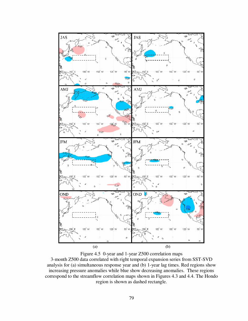
79
Figure 4.5 0-year and 1-year Z500 correlation maps
3-month Z500 data correlated with right temporal expansion series from SST-SVD analysis for (a) simultaneous response year and (b) 1-year lag times. Red regions show increasing pressure anomalies while blue show decreasing anomalies. These regions
correspond to the streamflow correlation maps shown in Figures 4.3 and 4.4. The Hondo region is shown as dashed rectangle.

80
Figure 4.6 2-year and 3-year Z500 correlation maps
Same as Figure 4.5 except showing (a) 2-year and (b) 3-year lag times.

81
Figure 4.7 0-year and 1-year U200 correlation maps
Same as Figure 4.5, but for 3-month U200 correlation values showing the (a) simultaneous response and (b) 1-year lag times.

82
Figure 4.8 2-year and 3-year U200 correlation maps
Same as Figure 4.7 but for (a) 2-year and (b) 3-year lag times.
83
Therefore, the Hondo appears to be significant during the JFM interval for the
simultaneous year, as well as the 1st, and 2nd lag years. It is also important to point out
that the 3rd year shows the Hondo as significant as part of the Z500 correlation analysis,
but the SST and U200 analysis show significant regions being in the western tropical
Pacific Ocean and central Pacific Ocean respectively. The ‘disaggregation’ of the
significant regions in the 3rd year is explained in the following section.
4.4 Discussion
4.4.1 Climatology
In order to provide a context for a discussion about the results, Figure 4.9 was
created to show the mean climatology data (1968 – 1997) of the U200, and SLP data
created using the online NCEP/NCAR Reanalysis plotting tool located at
http://www.esrl.noaa.gov/psd/cgi-bin/data/composites/printpage.pl. The black and white
dashed line on Figure 4.9 depicts the location of the jet core winds greater than 20 m/s.
In general, the U200 climatology maps (Figure 4.9a) shows that the East
Asian Jet Stream (EAJS) remains relatively weak (~25 m/s) and somewhat north during
the summer months of each year – essentially permitting the North American Jet Stream
(NAJS) to transport tropical air into the U.S. During the winter months the EAJS
increases in intensity (up to ~65 m/s) and shifts southward until reaching the approximate
location of the Hondo region. Though Figure 4.9a shows the U200 jet core (>20 m/s)
joining the EAJS and the NAJS, the EAJS splits into a northerly component, which joins
the Aleutian low, and a southerly component which joins with the NAJS on its journey
across the southern U.S. (hence the southerly dip in the jet core). The fact that the EAJS

84
Figure 4.9 Zonal wind field (a) and sea level pressure (b) climatology maps.
Climatology mean taken from (1968 – 1977)
is the primary driver of storm tracks toward the U.S. west coast was demonstrated in
work by Athanasiadis et al (2010) and many earlier works, and the bifurcation of the
EAJS was previously observed and described by Yang et al (2002).
Assisting with this process is the changing subtropical high off the west coast of
the U.S. as well as the deepening of the Aleutian low. During the summer months the

85
weakened EAJS is directed northward by the high pressure dome located off the western
coast of the U.S. As summer turns to winter the subtropical high decreases while the
Aleutian low becomes deeper and larger. The wintertime circulation patterns observed in
Figures 4.3 – 4.8 demonstrate that they are associated with an enhanced EAJS and a
decreased subtropical gyre.
Rasmussen and Wallace (1983) helped contrast the climatology with the impacts
of the 1983 El Niño event. They showed, for this particular El Niño event, the EAJS
extending further into the Pacific Ocean before beginning to disaggregate, thereby
carrying more of the storm energy directly toward the central west coast of the U.S. and
on to the CRB. Their work helped demonstrate that the concentration and intensity of the
EAJS contributed to the most extreme CRB water year of the last century.
Other work (e.g., Tootle et al, 2009) showed how there were some similarities
between the ENSO signal predicted for the 2009-2010 Niño 3.4 anomalies, and those
observed from past El Niño events – including the 1983 and 2003 events. Interestingly
enough the 2009-2010 event was relatively typical as far as its impact on the CRB, the
1982-83 event was the most extreme, and the 2002-03 was the least extreme on record.
The contrast between the winter of 1982-83 and 2002-03 can be observed on Figure 4.10.
The JFM zonal wind was only slightly greater than climatology, and the west coast
pressure dome was only marginally lower than climatology. It appears that these two
factors contributed to making the 02-03 El Niño event appear like an average water year.
In fact it brought the least amount of rainfall of any El Niño event in the last 60 years, a

86
Figure 4.10 Comparison between 1983 and 2003 ENSO Events
Showing (a) mean U200 JFM values from 1983, (b) mean U200 JFM values from 2003, (c) mean SLP JFM values from 1983, and (d) mean SLP JFM values from 2003. Dashed white line represents the dominant location (>20m/s) of the jet stream, and dashed box,
the Hondo region.

87
phenomenon coincident with the quasi-decadal drought cycle as shown in Wang et al.
(2009). This information helps demonstrate that the circulation patterns can operate
somewhat independently of the ENSO signal, and therefore, need to consider other
factors when assessing climate impacts on the CRB.
4.4.2 The Lagged Relationship
Understanding the climatology, it can now be seen that the SVD and correlation results in
a proper light. The results from the SST-SVD analysis show a significant covariance
region corresponding to the location of the EAJS as well as the associated atmospheric
circulation patterns observed in the Z500 analysis and in the SLP climatology maps. In
addition to this, there is a noticeable ENSO-like pattern which appears even though the
ENSO does not have a significant relationship with the upper CRB (Dettinger et al.,
1998; Rajagopalan and Lall, 1998). This ENSO Pattern is not observed in any of the
lagged response years, but the Hondo remains identifiable. Therefore one may ask: Are
the regions identified in the lagged analysis part of another climate cycle acting on the
CRB, of are they simply the results of a statistical analysis?
Research by Wang et al (2009, 2010b, 2010c) (hereafter referred to as W09,
W10b, and W10c respectively) helps to answer this question. Examining the observed
10-20 year cycle in precipitation over the intermountain west, W09 demonstrate that
within the transition phase of the Pacific Quasi-Decadal Oscillation (PQDO) there is a
lagged relationship between pacific SST’s and observed precipitation in the
intermountain west (It is important to note that the PQDO referred to in this paper is not
the same as that defined by Mantua and Hare (2002), but the result of work by Zhang et
al. (1997b) which is the first principle component of the Pacific Ocean SST’s from 25˚ S

88
to 60˚ N, which contains the variation from the tropics). Specifically, the analysis in
W09 suggests that the PDO cycle leads the intermountain precipitation cycle by 3-4
years.
The research in (W10b) tested the applicability of the 10-20 year climate cycle to
a surface water hydrology question, namely: what is the cause behind the prominent
coherence between the central tropical Pacific SSTs and the surface elevation of the
Great Salt Lake (GSL)? The results of this work reaffirmed the 3-year lagged response
between pacific SSTs and precipitation and furthered demonstrated a 3-year lagged
response in the GSL elevation following the precipitation. This process leads the GSL to
lag the central tropical Pacific SST variations by a half phase (~6 years) of the quasi-
decadal cycle of the PQDO. The result of W10b suggests that precipitation fluctuations
near the CRB are more strongly influenced by non-extreme ENSO periods rather than by
the typical, strong ENSO events.
Comparing the results obtained in W10b with the SST-SVD results from this
paper, it becomes apparent that the Hondo region reveals persistent responses in three
consecutive lags (0-2) but dissipates in lag 3. Figure 4.4b, while showing a significant
region stretching from the western tropical Pacific region into the Hondo, also shows the
significance of the central equatorial Pacific Ocean becoming significant (a pattern which
is also identified in Figure 4.8b. In other words, it appears that the reason the Hondo SST
is no longer significant by the third lag year is that it has past the typical 3 year influence
period of the PQDO. The comparison of these two papers appear to show that the
significance of the Hondo region, which is also observed during the transition phases of
89
the PQDO (W10b), can be explained as an intermediate cycle falling in between the
inter-annual ENSO events and the slow-varying PQDO cycles.
Additional work in W10c helps solidify this conclusion, by showing that the
Hondo may induce an atmospheric wave train which has a direct relationship with the
CRB during transition phases. Firstly, the 3-year lag time between the Pacific SSTs and
the intermountain precipitation was established by analyzing the water vapor budget over
the Great Basin. This examination identified that the water vapor flux convergence (one
of the terms in a water vapor budget) is the primary contributor to precipitation over the
Great Basin, requiring transient activity (e.g., cyclone waves) to occur in the right place.
Therefore an empirical orthogonal function (EOF) analysis was performed using the
gridded moisture flux potential data over the Pacific Ocean. The coherence between the
Pacific SSTs and the first mode (EOF1) of the moisture flux potential are highly
correlated. Likewise the Pacific SSTs are also highly correlated with EOF2, but at a 3-
year lag time. In other words the primary modes of the atmospheric moisture budget are
associated with Pacific SSTs leading the Great Basin precipitation by about 3 years.
The way that the SVD analysis contained in this research coincides with the
physical connection between the Great Basin precipitation and the PQDO identified in
W10b and W10c. In particular, the important role of the Hondo SST variability and its
associated teleconnection wave train, as were shown in W10c, are both similar to those
revealed in the SVD analysis and the circulation patterns throughout lags 0-2 (Figures
4.4-4.8). Along its path the Hondo is visible as a component of this short wave train (see
Figure 2b of W10c) which induces anomalous low pressure to the west of the
Intermountain region. The location of the starting point of the short-wave train not only

90
helps to explain Hondo’s existence and importance, but it explains why the western
tropical Pacific Ocean region shown in Figure 4b (JFM interval) is significant as well.
Therefore the Hondo is simply one component on a track of regions responsible for
transporting moisture from the tropics to the CRB.
Another insight into the reason for the 1-year lag of the Hondo (and the
diminishing 2-year lag as well) is the fact that because the Hondo is part of the wave train
during the winter months (JFM) of transition years (non-extreme ENSO years), it should
have a stronger signal with the CRB during periods when the ENSO is not impacting
climate signals in the Pacific Ocean. Since the ENSO signal is short-lived, the Hondo
appears at longer lead times because it is always a part of the mechanism transporting
moisture to the CRB. By the 3-year lag time the persistence of the Hondo is superseded
by the signal coming from the central equatorial Pacific Ocean (i.e. the QDO). This
demonstrates that while ENSO remains a considerable factor affecting the CRB, the
Hondo is a “new” factor that has a sustained effect on the CRB streamflow for up to three
years. This finding strongly suggests the potential for an extended range of streamflow
prediction.
4.5 Summary and Conclusions
The connection between the Hondo and the CRB streamflow is identified through
two avenues in this paper. First, the SVD analysis of SST, as well as the correlation
analysis with the Z500 and U200 data, showed that the SST-CRB connection identified in
Lamb et al (2010) and Aziz et al (2010) exists in the atmospheric data at similar lag
times. This analysis demonstrated the connection between the Hondo was not simply a
statistical relationship between two independent variables, but a result from the
91
covariability of the Pacific Ocean and the atmospheric circulation through the so-called
teleconnection.
The second way the Hondo-CRB connection was identified was by understanding
the physical connection behind the lagged response between the two datasets. The work
provided by Wang et al., (2009, 2010a, 2010b) helped identify the quasi-decadal cycle
embedded in the Pacific Ocean and the fact that the precipitation in the inter-mountain
west region is on a similar cycle, but lags 3-years behind the SST cycle. The physical
connection between the Pacific Ocean and the precipitation was outlined by identifying a
similar 3-year lag in the first two principle components (EOF1 and EOF2) of the filtered
moisture flux stream function. EOF1 was highly correlated with the SST cycle while
EOF2 was highly correlated with the precipitation cycle.
The utility of this research is to create the technical confidence needed to use the
Hondo as a potential tool for creating long-lead forecasts of the CRB streamflow. The
National Weather Service utilizes an Extended Streamflow Prediction (ESP) software
tool that employs historic temperature and precipitation time series to generate an
ensemble of future streamflow scenarios. Knowledge about the lagged relationship
between the Hondo and the CRB can be used to weigh the ESP output, essentially adding
a “long-lead cycle” bias to the historical data. The result of this work has the potential to
improve the long-lead forecast ability for the CRB.

92
CHAPTER 5
TESTING A POST-ANALYSIS WEIGHTING TECHNIQUE TO IMPROVE LONG-
LEAD FORECASTS OF THE COLORADO RIVER BASIN
5.1 Introduction
The National Weather Service’s (NWS) Colorado Basin River Forecast Center
(CBRFC) issues regulated water supply forecasts for the Colorado River Basin on a
monthly basis. Each month the forecast includes streamflow volumes expected for the
following three months. During the winter and spring months, the typical 3-month
forecast is accompanied by the season spring runoff forecast, given as a 4-month lump
sum volume for the April – July period. In addition to these official forecasts the CBRFC
produces a yearly outlook on August 1 and October 1 for a given water year for the
following water year. These forecasts represent the best estimate of water resource
supply in the Colorado River Basin (CRB), and are created using the Extended
Streamflow Prediction (ESP) software.
Water resource managers at the U.S. Bureau of Reclamation (USBR) use the
forecasts created by the CBRFC to model the next 24-months of resource storage,
releases, and diversions in order to predict future reservoir levels and plan for hydro-
power generation supply. Since the CBRFC forecasts run at most for 12 months and the
USBR creates a 24-month projection of water usage, the USBR must make estimates of
the last 12 months of the 24 month projection. This estimate is partially made by
extrapolating information from the CBRFC forecasts and the remainder is filled with the
30-year mean streamflow observed from 1971 – 2000. Therefore an improvement to the

93
status quo is to identify climate patterns which can increase the accuracy of the long-lead
(> 1 year) streamflow forecasts in the CRB.
The utility of long-lead forecasts based on climate has been introduced and
assessed in previous research. For example, because of the prominence of the El Niño
Southern Oscillation (ENSO) signal on streamflow in the western United States, the
related indices explaining the ENSO have appeared in many studies (Piechota and
Dracup 1996; Piechota et al. 1997; Hamlet and Lattenmeier, 1999; Clark et al. 2001;
McCabe and Dettinger 2002; Werner et al 2004; Grantz et al, 2005). However McCabe
and Dettinger (2002) as well as Werner et al (2004) demonstrated that the ENSO has very
little impact on CRB streamflow, because of the weak correlation with the upper CRB
river gauges. Therefore if the ENSO signal can not enhance the long-lead streamflow
forecasts, then which other climate data can be used?
The current paper builds upon recent research (Lamb et al, 2010a; 2010b; Aziz et
al, 2009) which shows there is an area of the Pacific Ocean (hereafter referred to as
Hondo) which demonstrates a significant correlation with streamflow in the Colorado
River Basin (CRB). Both Lamb et al. and Aziz et al. identified this region using a
singular value decomposition analysis. In both cases the level of significant covariance
was determined by finding regions whose covariance exceeded the 95% significance
level of the correlation coefficient. Lamb et al (2010a) show the influence of Hondo
when comparing the winter time SST’s of Hondo from a given water year, with the total
yearly streamflow of the following water year. Aziz et al. show a similar Hondo pattern
when comparing SST and snow water Equivalent (SWE) data from the Rocky Mountains
in the U.S. with a year lag. Finally, Chapter 4 demonstrated that the Hondo is connected

94
to streamflow in the CRB during the winter months through an enhanced jet stream and
decreased subtropical gyre on the west coast of the U.S.
Because the ESP output is an ensemble of possible streamflow scenarios for
representing a given forecast period, it is possible to weigh the output and thereby
introduce a climate-based bias in order to create a new forecast value. Work by Werner
et al (2004) proposed to do this using climate index data based on the ENSO signal, in
order to improve the spring runoff forecasts of the CRB based on climate observations
from the previous fall or summer.
Because the ENSO signal is weak in the CRB, the existing research has provided
the foundation for using the Hondo as a basis for forecasting the streamflow. Therefore,
the proposed research aims to determine the 3-month interval, lag time, and weight kernel
required to optimize the forecast skill score. The forecast skill scores used are the root
mean squared error (RMSE) and the Linear Error in Probability Space (LEPS) score.
Both are used since the RMSE is a parametric assessment with a long history of
application, while the LEPS score is a non-parametric assessment.
5.2 Data
5.2.1 Streamflow Data
The USBR maintains a spreadsheet of naturalized streamflow data for 29 gauges
within the CRB which can be obtained from the following URL
(http://www.usbr.gov/lc/region/g4000/NaturalFlow/current.html). Since a given water
year actually begins and ends in different calendar years, when this report refers to a
given water year (for example, 1996) it is referring to the period October 1, 1995 through
September 30, 1996. Therefore when the total yearly streamflow of a given water year is

95
shown, this is referring to the total water volume observed at a given gauge from October
1 through September 30 of the specified calendar year. In order to maintain some
continuity between the previous and current work, this data set is used here because it
was used in both papers by Lamb et al (2010a and 2010b). The 29 locations are displayed
on Figure 5.1.
5.2.1 Sea Surface Temperature Data
The SST data used in this research is a subset of the gridded data developed by Smith et
al (2008). The data is available online at (http://www.ncdc.noaa.gov/oa/climate/research/
sst/ersstv3.php) through the National Oceanic Atmospheric Administration (NOAA)
National Climate Data Center (NCDC). The SST data are converted into Excel format
using software, named Ocean Temperature Analysis (OTA), developed at UNLV
specifically for this purpose. The Smith SST dataset is a 2º x 2º monthly mean gridded
dataset existing from January 1854 through the present day. The subset of this data is
defined to represent the boundary of the Hondo region (i.e. 150 E – 200E, 34N – 24N) as
defined by Aziz et al (2010). The mean SST anomaly value for this region is the Hondo
index value.
As previously mentioned, the current research showing the Hondo-CRB
correlation demonstrates a lag time of more than a year between the changes in
temperature and the streamflow. Specifically, the research by Lamb et al (2010a),
showed that the 3-month average SST intervals of January-March, and February-April
from a given water year, has a significant correlation with streamflow variation for the
following water year volume. Other research into the strong winter monsoon from
northeast Asia (Zhang et al, 1997a) showed that east Asian jet stream passes over the
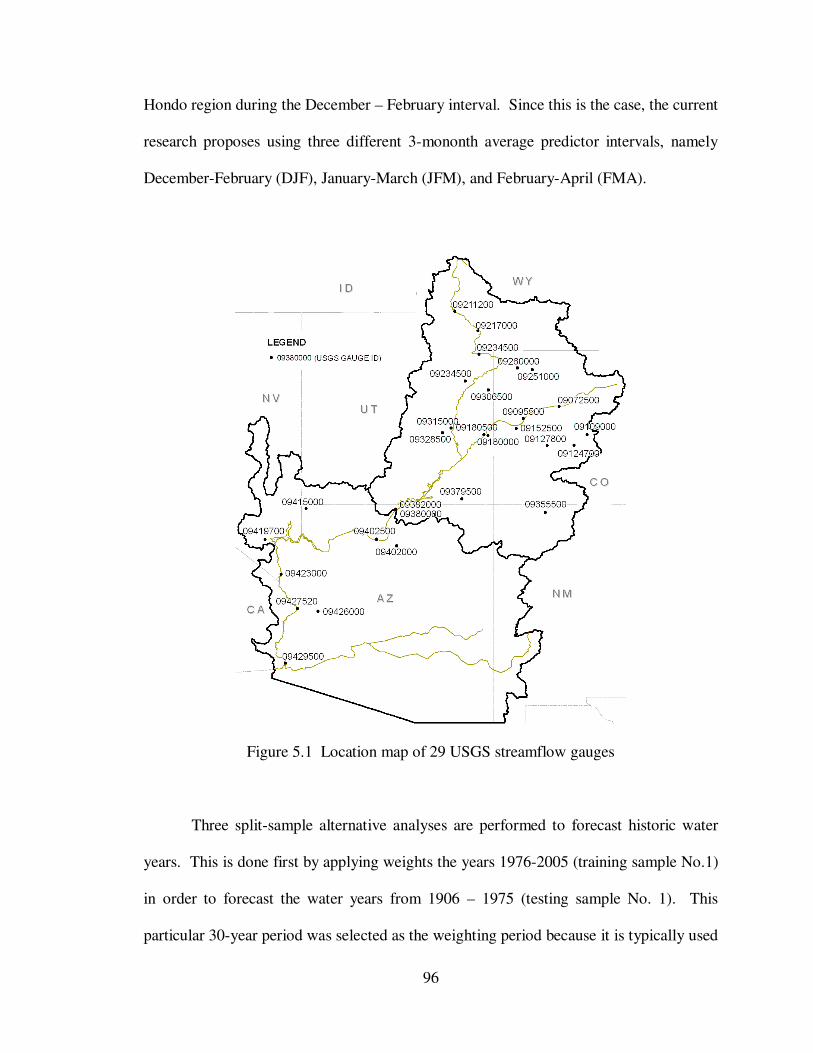
96
Hondo region during the December – February interval. Since this is the case, the current
research proposes using three different 3-mononth average predictor intervals, namely
December-February (DJF), January-March (JFM), and February-April (FMA).
Figure 5.1 Location map of 29 USGS streamflow gauges
Three split-sample alternative analyses are performed to forecast historic water
years. This is done first by applying weights the years 1976-2005 (training sample No.1)
in order to forecast the water years from 1906 – 1975 (testing sample No. 1). This
particular 30-year period was selected as the weighting period because it is typically used

97
by the NWS's Colorado Basin River Forecast Center to calibrate their ESP software. The
ESP produces output streamflow traces which are based on the temperature and
precipitation data from the years 1976-2005. In order to test the sensitivity of the
selection of training and testing sample, the second split-sample alternative is performed
using 1906 – 1955 as the training sample to forecast the water years of 1956 – 2005.
Finally the third alternative uses 1956 – 2005 as the training sample to forecast the water
years from 1906 – 1955. The years of data selected for Alternatives 1 and 2 were chosen
simply to provide forecasts for the 100 year period stretching from 1906 through 2005.
5.3 Methodology
The forecasts in this work are created using a kernel, to weigh the streamflow at
three different lag times: 0-year (simultaneous year), 1-year, and 2-year lags. For
example, if a forecast for the 0-year lag is to be created for the 1920 water year the
Hondo value from JFM 1920 is compared to the JFM Hondo values from all the years in
the training sample. The difference between the 1920 Hondo value and the values of the
training set are calculated, sorted in ascending order and then ranked. The difference, or
rank, is the primary information used in the weight kernel calculation. Once the kernels
are calculated all of the weights for a given year are proportioned so that their sum equals
one. Since this process is based on the DJF, JFM and FMA intervals then there are three
different sets of weight kernels produced.
Because the differences between all forecast years and all training years are
calculated at the start, the lag time for the forecast comes from selecting the appropriate
weight vector when the forecast value is generated. For example if the 1920 water year is
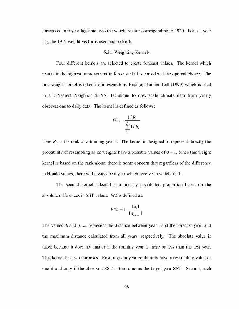
98
forecasted, a 0-year lag time uses the weight vector corresponding to 1920. For a 1-year
lag, the 1919 weight vector is used and so forth.
5.3.1 Weighting Kernels
Four different kernels are selected to create forecast values. The kernel which
results in the highest improvement in forecast skill is considered the optimal choice. The
first weight kernel is taken from research by Rajagopalan and Lall (1999) which is used
in a k-Nearest Neighbor (k-NN) technique to downscale climate data from yearly
observations to daily data. The kernel is defined as follows:
1
1/1
1/
ii n
i
i
RW
R=
=
∑
Here Ri, is the rank of a training year i. The kernel is designed to represent directly the
probability of resampling as its weights have a possible values of 0 – 1. Since this weight
kernel is based on the rank alone, there is some concern that regardless of the difference
in Hondo values, there will always be a year which receives a weight of 1.
The second kernel selected is a linearly distributed proportion based on the
absolute differences in SST values. W2 is defined as:
,max
| |2 1
| |i
i
i
dW
d= −
The values di and di,max represent the distance between year i and the forecast year, and
the maximum distance calculated from all years, respectively. The absolute value is
taken because it does not matter if the training year is more or less than the test year.
This kernel has two purposes. First, a given year could only have a resampling value of
one if and only if the observed SST is the same as the target year SST. Second, each

99
successive weight is distributed on a roughly linear, but negative, sloping line so that year
i has only slightly more weight than year i+1. However, since the behavior of this kernel
is a decreasing linear distribution of weights, then there is a chance that it will give too
much weight to years which are not actually “near” to the target year.
The third weight, W3 is given as the inverse distance squared weight:
2
13i
i
Wd
=
Once again, di is the difference between the training year and the forecast year. Because
the theoretical values of W3 range from -∞ to ∞, the weights for each forecast year are
proportioned so that values range between 0 and 1 and their sum is equal to 1. This
weight kernel has a plotted behavior similar to W1 except that it gives even less weight to
observations with increasing values of di. Since this kernel does shift the majority of the
weight to the first or second years some relevant information from other years may be
ignored.
The final kernel, W4 is simply the inverse distance:
14i
i
Wd
=
Both W3 and W4 are commonly used kernels used in resampling and interpolating
applications or as comparisons to other more sophisticated methods. W4 does not weigh
the closest 1 or 2 as heavily as W1 or W3, but since it is not linear it also does not
distribute the weights to too many of the other, adjacent observations.
Weights are calculated using the raw SST values. A test was run to see if there
would be any difference between using raw data and calculating the Hondo anomalies
which were used in the SVD analysis (Lamb et al. 2010, Aziz et al,. 2010). The results of

100
this simple test demonstrated that there was no significant difference between the forecast
skill score resulting from these two data sets. Additionally, using proportioned weights
were compared to raw (un-proportioned) weights to see if the forecast skill is sensitive to
either method. The results of this test demonstrated that there was no significant
difference. From these two small tests the use of the raw Hondo data is selected for
testing because it is simpler to employ, and the proportioned weights are used because
they communicate the idea of resampling probability better than the raw weights.
5.3.2 Forecast Development
Forecasts are created using the weight vector in a weighted bootstrap procedure,
where 1000 re-sampled values are taken from the training set. The mean value of each
re-sampled set is calculated and then the mean of all these means is calculated to arrive at
the forecast value. The weighted bootstrap is a method has been used extensively in a
variety of fields (Efron 1979, 1982). Typically the bootstrap method is used to estimate a
population parameter from a sample dataset. However, in this application, the goal is to
add a bias to the training dataset which reflects the link between known climate
conditions and CRB streamflow.
Forecast values are calculated for a given split sample alternative, 3-month
period, weight kernel, and lag time. Each combination of alternative-period-kernel-lag
represents a single forecast scenario. Since there are three split-sample alternatives, three
3-month periods (DJF, JFM, and FMA); four weight kernels (W1, W2, W3 and W4); and
three lag times (0, 1, or 2 years) there are a total of 108 forecast scenarios (3 x 3 x 4 x 3).

101
5.3.3 Forecast Skill Scores
Assessing the forecast skill is assessed using the root mean squared error (RMSE)
and the linear error in probability space score (LEPS) scores. Relative error (Abramowitz
and Stegun, 1972) is also used here as a quick way of assessing the error of a forecast by
comparing the forecast error to the observed value using the following equation:
, , ,
, ,
1y l y l y l
y l y l
F O FRE
O O
−= = −
Here the forecast, F at streamflow location, l, and year, y, are compared to the
observation, O of same location and year. The RE is used here to create a time series plot
of the forecasts errors, in order to identify periods of weak forecasting ability. The utility
of the RE is not only to provide an indication of how close a given forecast is to the
observation value (as a percent fraction of the observed) but also to give an indication of
the bias in the forecast method. Since the RE is calculated for each year and location, the
mean forecast bias is computed at each location for a given forecast scenario.
The RMSE is widely used to assess forecast errors (Wilks, 2006). A strength of
the RMSE is its simplicity in communicating the forecast error in the same units as the
forecasts themselves. However, the RMSE assumes that the forecast errors are
distributed normally and it is therefore sensitive to forecast error variance. This makes it
difficult to interpret the RMSE results as there is no consistent relationship between the
RMSE and the average error of forecasts.
The RMSE is not be reported directly. Since the current method of modeling
CRB streamflow projection uses the 1976-2005 mean for the long-lead forecasts, then a
skill score based on the forecast RMSE and the climatology RMSE (1976-2005) is
calculated. The skill score formula is given as

102
1f
RMSE
c
RMSESS
RMSE= −
This equation is used to demonstrate the relative improvement of the forecast method
(RMSEf) over the climatology (RMSEc). RMSEc is calculated by finding the RMSE using
the 1976-2005 mean as the forecast value for all years at a given streamflow location.
Also used to asses forecast skill is the Linear Error in Probability Space score
(Ward and Folland, 1991; Potts et al, 1996). The LEPS score is used here because it does
not assume that the errors have a defined distribution. The LEPS score gives a higher
score for forecasts which predict extreme events, as opposed to forecasts of observed
values which are closer to the mean. The work by Potts revised the LEPS score by Ward
and Folland to remove a “bending back” problem when forecasting a continuous variable,
as is the case in this research.
The basic concept of the LEPS score is to compare the forecast point with the
observed data inside probability space. To complete this task we generate an empirical
cumulative distribution function (eCDF) from the observed data. The eCDF is created
from the streamflow data used as the testing set. In other words the first split sample
analysis uses observed streamflow from years 1906-1976 create the eCDF (n1 = 70), the
second split sample analysis uses 1956-2005 (n2 = 50), and the third uses 1906-1955 (n3
= 50). The eCDF gives a weight of 1/n to each observed value. Since there are 100
observation points at each streamflow gauge, the y-axis of the eCDF is defined by a
vector P, where P = q/101 as ‘q’ goes from 1 to 100. P does not include the points '0' or
'1' in order to ensure that there can be forecast values interpolated below and above the
range of observed streamflow values at a given location.

103
The LEPS score is calculated from the following formula as developed by Potts et
al (1996):
2 23(1 | | ) 1f o f f o oLEPS P P P P P P= − − + − + − −
where Pf and Po represent, respectively, the probabilities of the forecast and observed
streamflow values. The values of Pf and Po are read from the eCDF, (see Figure 2) for a
given forecast year y, and location l. Values of the LEPS score range from -1 to 1.5.
Figure 5.2 Schematic showing how Pf and Po are obtained from the eCDF
5.3.4 Average Skill Score
The goal of the average skill score is to summarize the LEPS scores obtained at a
given location, for all forecast years, and express this skill in terms of a percentage
improvement (or decline) with respect to using the mean as the forecast value. The
average skill score (Potts et al., 1996) is found by dividing the sum of all LEPS scores at
a given location by the sum of the maximum possible, or minimum possible, LEPS scores
as determined by the following equation:
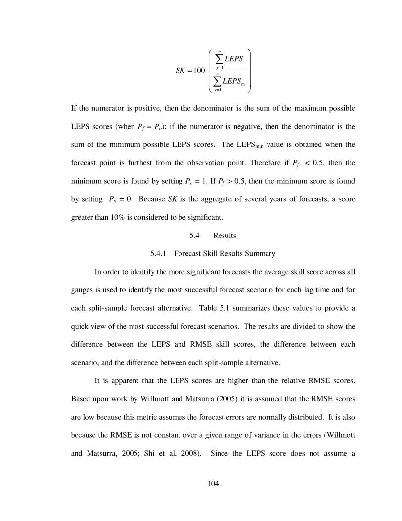
104
1
m1
100
n
y
n
y
LEPS
SK
LEPS
=
=
= ⋅
∑
∑
If the numerator is positive, then the denominator is the sum of the maximum possible
LEPS scores (when Pf = Po); if the numerator is negative, then the denominator is the
sum of the minimum possible LEPS scores. The LEPSmin value is obtained when the
forecast point is furthest from the observation point. Therefore if Pf < 0.5, then the
minimum score is found by setting Po = 1. If Pf > 0.5, then the minimum score is found
by setting Po = 0. Because SK is the aggregate of several years of forecasts, a score
greater than 10% is considered to be significant.
5.4 Results
5.4.1 Forecast Skill Results Summary
In order to identify the more significant forecasts the average skill score across all
gauges is used to identify the most successful forecast scenario for each lag time and for
each split-sample forecast alternative. Table 5.1 summarizes these values to provide a
quick view of the most successful forecast scenarios. The results are divided to show the
difference between the LEPS and RMSE skill scores, the difference between each
scenario, and the difference between each split-sample alternative.
It is apparent that the LEPS scores are higher than the relative RMSE scores.
Based upon work by Willmott and Matsurra (2005) it is assumed that the RMSE scores
are low because this metric assumes the forecast errors are normally distributed. It is also
because the RMSE is not constant over a given range of variance in the errors (Willmott
and Matsurra, 2005; Shi et al, 2008). Since the LEPS score does not assume a

105
distribution for the errors its scores are not affected in the same way as the RMSE.
However, the LEPS score rewards forecasts of extreme values more than forecasts of
values closer to the mean. Therefore the individual LEPS score results must also be
examined further.
Table 5.1 Summary of successful scenarios based on LEPS and RMSE scores.
It is apparent that the LEPS scores are higher than the relative RMSE scores.
Based upon work by Willmott and Matsurra (2005) it is assumed that the RMSE scores
are low because this metric assumes the forecast errors are normally distributed. It is also
because the RMSE is not constant over a given range of variance in the errors (Willmott
and Matsurra, 2005; Shi et al, 2008). Since the LEPS score does not assume a
distribution for the errors its scores are not affected in the same way as the RMSE.
However, the LEPS score rewards forecasts of extreme values more than forecasts of
values closer to the mean. Therefore the individual LEPS score results must also be
examined further.
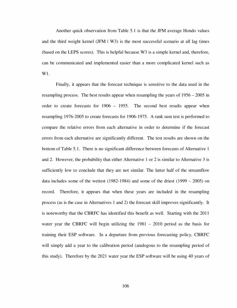
106
Another quick observation from Table 5.1 is that the JFM average Hondo values
and the third weight kernel (JFM | W3) is the most successful scenario at all lag times
(based on the LEPS scores). This is helpful because W3 is a simple kernel and, therefore,
can be communicated and implemented easier than a more complicated kernel such as
W1.
Finally, it appears that the forecast technique is sensitive to the data used in the
resampling process. The best results appear when resampling the years of 1956 – 2005 in
order to create forecasts for 1906 – 1955. The second best results appear when
resampling 1976-2005 to create forecasts for 1906-1975. A rank sum test is performed to
compare the relative errors from each alternative in order to determine if the forecast
errors from each alternative are significantly different. The test results are shown on the
bottom of Table 5.1. There is no significant difference between forecasts of Alternative 1
and 2. However, the probability that either Alternative 1 or 2 is similar to Alternative 3 is
sufficiently low to conclude that they are not similar. The latter half of the streamflow
data includes some of the wettest (1982-1984) and some of the driest (1999 – 2005) on
record. Therefore, it appears that when these years are included in the resampling
process (as is the case in Alternatives 1 and 2) the forecast skill improves significantly. It
is noteworthy that the CBRFC has identified this benefit as well. Starting with the 2011
water year the CBRFC will begin utilizing the 1981 – 2010 period as the basis for
training their ESP software. In a departure from previous forecasting policy, CBRFC
will simply add a year to the calibration period (analogous to the resampling period of
this study). Therefore by the 2021 water year the ESP software will be using 40 years of

107
historical inputs (1981 – 2020) to create forecasts (Personal Communication Kevin
Werner, CBRFC; May 2010).
5.4.2 Forecast Skill Maps
In order to identify the region of increased or decreased forecast skill, the top
forecast scenarios, for each lag time and for all three alternatives, are mapped and
displayed on Figure 5.3. This figure displays nine (9) maps showing the average LEPS
skill scores at each of the streamflow locations in the basin. The first row of maps on
Figure 3 (a – c), representing Alternative 1, show that for the upper reaches of the Green
River, the forecast skill does not show a significant improvement. Along the headwaters
of the Colorado and Gunnison Rivers there are a few positive results, and in the lower
CRB there are only few significant improvements for gauges not along the Colorado
River itself. This pattern is generally repeated for each alternative and for each lag year,
except for Alternative 3, which generally shows a weak pattern of forecast skill results at
0 and 1-year lag times.
Despite the results of the rank sum test from the previous section, Figure 5.3
shows an observable difference between the forecast skill results of Alternative 1 and 2.
For example, Figure 5.3d shows Alternative 2 providing an improved forecast approach
in the upper CRB - especially along the headwaters of the basin. It also shows that the
skill diminishes as the lag time increases, and that the number of gauges showing
successful forecasts also diminishing. It is expected that the forecasts would demonstrate
their highest skill scores at the 1 year lag time because of the interference that shorter,
more intense climate cycle have upon the basin. Even though the results are not expected

108
Figure 5.3 Maps showing average skill score results.
Non-significant results (<10%) displayed as black dots. Figures a-c represent the results from the 1st split sample alternative (Alt 1), d - f Alt. 2, and g - i Alt. 3. The first column
(Figures a, d, g) are the 0-lag forecasts, the second column (b, e, h) are the 1-year lag forecasts, and the third column (c, f, i) are the 2-year lag forecasts.

109
they seem to make more sense by showing a decreasing and diminishing ability to use the
Hondo as a basis for generating forecasts.
5.4.3 Forecast Time Series
Because the average skill score is a composite of all the forecasts generated at a
location, it is necessary to investigate the individual forecast values to determine if the
LEPS scores are higher because they give more weight to successful forecasts of extreme
values and if there are identifiable patterns in the forecast’s successes or failures. Figures
5.4 and 5.5 display scatter plots comparing the forecast and observed values at the 1-year
lag time from Alternative 2 and 3 respectively. The correlation value for each scatterplot
is displayed in the lower right-hand corner of each plot.
The main observation from Figures 5.4 and 5.5 is that there are few gauges where
the correlation between the forecast and observed is significant at the 95% level (i.e. r >
0.273) While these figures show an overall performance, they do not explain if there are
certain periods of time where the forecasts perform better than others. Figure 5.6 – 5.8
display this observation better by plotting the forecast relative error from alternatives 2
and 3 onto a single time series plot. Figure 5.6 shows the forecast errors at eight gauge
locations for the 0-year lag time. Figures 5.7 and 5.8 show the same, except they show
the 1-year and 2-year lag times. The highlighted regions shown on these figures identify
periods where streamflow was below average at the Lees Ferry gauge (USGS ID
09380000) with less than two consecutive years of above average streamflow in between.
Figure 5.6 shows that, with the exception of (d), (f), and (h) there is a pattern to
the skill scores. For example the forecast skill is observed as more erratic for years
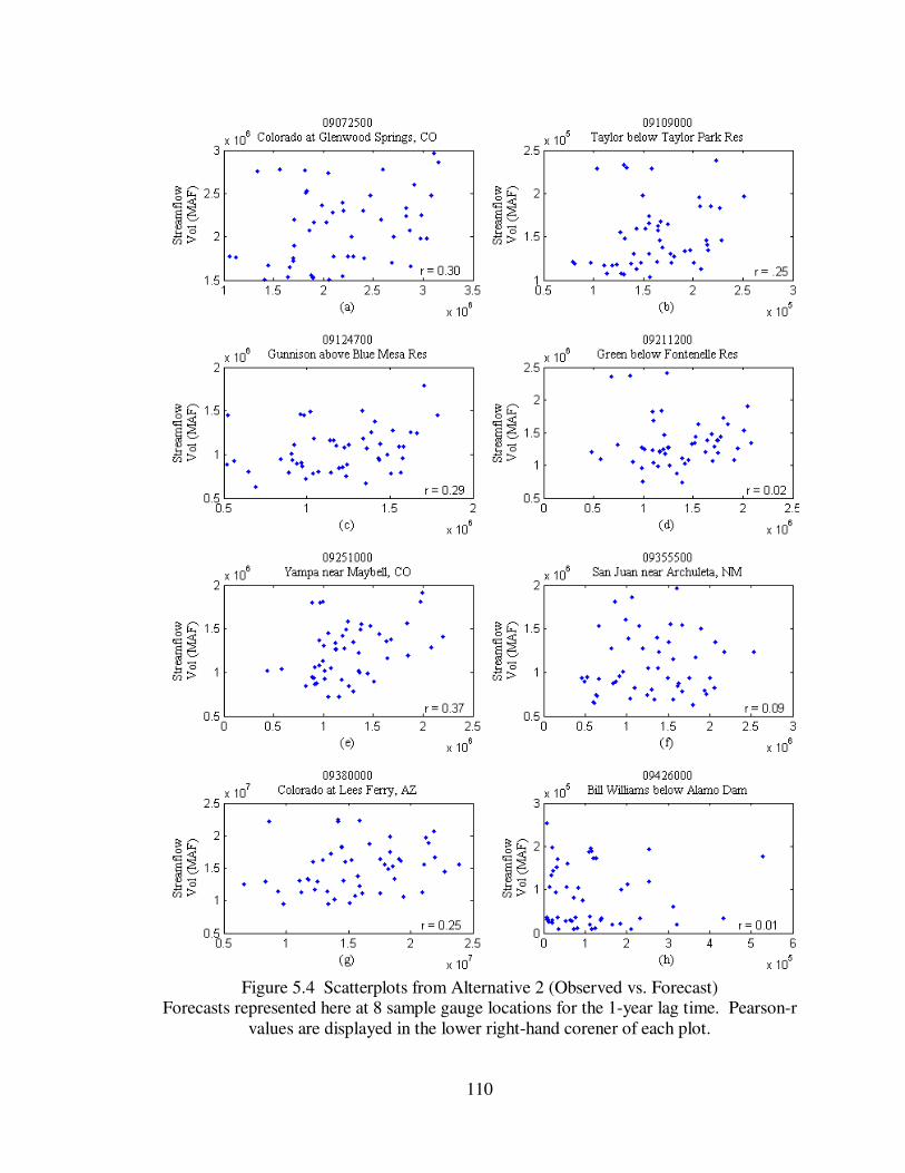
110
Figure 5.4 Scatterplots from Alternative 2 (Observed vs. Forecast) Forecasts represented here at 8 sample gauge locations for the 1-year lag time. Pearson-r
values are displayed in the lower right-hand corener of each plot.
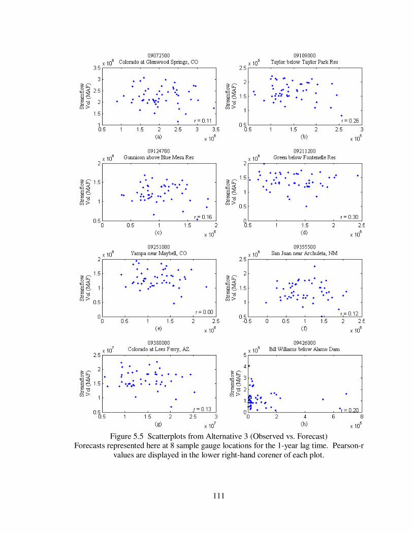
111
Figure 5.5 Scatterplots from Alternative 3 (Observed vs. Forecast)
Forecasts represented here at 8 sample gauge locations for the 1-year lag time. Pearson-r values are displayed in the lower right-hand corener of each plot.

112
Figure 5.6 0-year lag forecast relative errors for eight gauge locations
Figure displays relative error time series from alternatives 2 & 3 created from 0-year lag time. Shaded areas represent low-flow periods defined as below average streamflow with less than two consecutive years of above average streamflow. Pearson-r values for each
alternatives 2 and 3 are displayed in the lowers left and lowere middle of each plot, respectively.

113
Figure 5.7 1-year lag forecast relative errors for eight gauge locations Same as Figure 5.6 except showing the 1-year lag time.

114
Figure 5.8 2-year lag forecast relative errors for eight gauge locations Same as Figure 5.6 except showing the 2-year lag time.
115
highlighted as low flow years. In between these periods the forecast errors are
comparatively small and much less erratic (this appears to hold true for all location
except for the stations shown on Figure 5.6 – 5.8 (d), (f), and (h)). These periods
correspond to several of the driest years of the last century as shown by the highlighted
regions. For example (d), appears to show an inconsistent forecast skill until the early
1940’s. (f) shows that prior to the late 1920’s the forecasts worked well. However, after
1930 the forecast errors are very inconsistent. Finally, Figure (h) shows that the forecast
skill of Bill Williams River gauge is not acceptable for any period of time.
The poor forecast skill along the Bill Williams River is not surprising since this
location has the highest amount of streamflow variance in the CRB. The skill displayed
at the Green River station is also not surprising because the SVD analysis provided by
Lamb et al (2010b) showed how the upper reaches of the Green River are not always
significantly correlated with the Hondo region. There appears to be a limit to how far
north the Hondo can be applied, and perhaps this explains the low skill at the San Juan
River station.
Perhaps one reason there may be periods where the forecast skill is extremely
poor may be attributed to the change in significance of a particular climate cycle. While
climate cycles tend to appear with predictable amplitude and period, they can experience
periods of inactivity, where the amplitude of the cycle is noticeably dampened. Wang et
al (2010b) identified a quasi-decadal oscillation in Pacific Ocean SSTs which
demonstrated a significant correlation with precipitation in the intermountain west region
with the SSTs leading precipitation by 3-years. Lamb et al (2010b) identified that the
Hondo is part of the short-wave train which transports warm moist air from the tropical

116
Pacific Ocean toward the intermountain west. From 1900 – 1945 and from 1965 -
present the QDO behaves in a predictable manner (see Figure 4 of Wang et al, 2010b)
However, during the period from 1945 – 1965 the identified cycle was mostly inactive,
showing a diminished correlation with intermountain west precipitation. Therefore,
forecasts created from a single climate phenomenon will not always perform the same
simply because of climate variability.
5.5 Conclusions and Recommendations
The overall results of this work demonstrated that climate information can be
applied to weigh historical data in order to generate improved long-lead forecasts. This
approach was tested using streamflow data from the Colorado River Basin (CBR) in an
effort to find improved streamflow forecasts at lead times greater than one year. The
basis of this approach is rooted in an understanding of the long-lead climate trends
impacting the CRB.
Previous studies helped identify a region of the Pacific Ocean, named the Hondo,
which represents a portion of the atmospheric short-wave train which transports moist air
from the Pacific Ocean Tropics. The weighting technique used the mean, wintertime
SST values of the Hondo region to determine how similar a given forecast period is to all
of the historical data. Those historic years closest to the forecast period were weighted
more in a resampling technique designed to add a climate-bias into the forecasts. Several
different weight kernels were tested, and the inverse distance kernel demonstrated the
highest skill.
The results of this research show that it is possible to use known climate cycles as
a basis for generating forecasts at lead times of 1-year or greater. These results also

117
identify places for further study. For instance the observation that the periods where
forecast errors were unacceptably high also coincided with periods of below average
streamflow. It is hypothesize that this is because the current forecast technique does not
explicitly consider soil moisture in the formulation of the forecast. Though the soil
moisture state is implicit in the SVD analysis of Lamb et al (2010a), one improvement to
the current forecast method would be to apply this technique to forecasts produced by the
CBRFC’s ESP software. Since the ESP utilizes soil moisture as an input into their
physical model, weighing the ESP output based on climate relevance would incorporate
soil moisture states into this forecasting procedure and potentially increase the forecast
skill.

118
CHAPTER 6
CONTRIBUTIONS AND RECOMMENDATIONS
6.1 Contributions
The research completed in this dissertation presents several contributions to the
field of water resource engineering, including an improved understanding of how changes
in Pacific Ocean sea surface temperatures impact the Colorado River Basin (CRB), how
these changes are connected to the CRB, and how this knowledge can be used to improve
long-lead water supply forecasts.
Prior to this work, there was an understanding that the known influences of the El
Niño Southern Oscillation did not have a significant impact on the CRB. Therefore any
improvement to long-lead CRB water supply forecasts would have to come from an
improved understanding of how and where climate impacts CRB streamflow
Answering Question 1 identified a 1-year teleconnection between the Pacific
Ocean and the CRB. The region of the ocean with a significant correlation was located
from 35N – 25N and from 150E – 200E (160W). The Hondo, as this region was named,
had a negative correlation relationship with the CRB streamflow, meaning that
decreasing SSTs were correlated with increasing streamflow. This region was identified
in other research while studying SST impacts on drought conditions (Rajagopalan and
Lall, 2000), precipitation (Wang and Ting, 2000), and North Platte River streamflow
(Soukup et al., 2009). Each of these studies used different data, even different SST data,
and the Hondo region was identified as significant. A study performed at the same time
as Task 1 identified the Hondo when studying the impact of SSTs on snow water
equivalent measurements in the Rocky Mountains.

119
Question No. 2 sought to describe the physical connection between the wintertime
SST anomalies (i.e. Hondo anomalies) and the CRB. This analysis demonstrated that the
Hondo is correlated with the East Asian Jet Stream (EAJS). During the winter months
the EAJS passes across the southern tip of the main island of Japan, and enters the Pacific
Ocean over the Hondo, then bifurcates: the northern split joining the Aleutian low, and
the southern split dipping southward to join the North American Jet stream. This system
is also correlated with a significant low pressure system that develops in conjunction with
the intensity of the EAJS and Hondo SSTs in order to impact CRB streamflow. This
system was identified to be significant with CRB streamflow at 0, 1 and 2 year lag times.
By the third year the Hondo was no longer identified as significant.
Comparing this analysis with the current state of knowledge revealed that the
typical water year has a residual impact on the CRB because of the slow response of soil
moisture. The quasi-decadal oscillation (QDO) observed in the precipitation data was
shown to lead the QDO phase observed in the level of the Great Salt Lake by three years
(Wang et al, 2010b). This showed that the total surface hydrology response can have
around three years to respond to precipitation. Also, there is a quasi-decadal oscillation
in the Pacific Ocean (PQDO) which has a three year lead time correlation with the
precipitation QDO. The significant PQDO region is centered over the central tropical
Pacific Ocean; basically the existing Niño4 region.
Comparing the results from Task 2 with the current knowledge revealed that the
water supply from a given water year is impacted by, on average, the previous two (2)
water years. The mechanism creating this connection is explained by the wintertime
intensity of the EAJS and observed by the Hondo SST variability. By the third water

120
year the impact of the Niño4 region and the mechanism transporting moist air from the
tropical Pacific Ocean, becomes more significant than the Hondo mechanism. Therefore
the research completed by Task 2 identifies that there is a lagged relationship between the
Hondo and the CRB which is likely related to basin characteristics. The research also
identified that the CRB is also influenced by the PQDO at lag times of around 3 years.
The final task, answering question No. 3, used the Hondo as a basis for
forecasting streamflow in the CRB at 0, 1, and 2-year lag times. The results of this task
showed that the best forecast skill results appear when using the inverse distance weight
kernel, based on the January – March (JFM) Hondo values, to resample the training data
set. Tests also showed that forecasts are sensitive to which historical data are selected as
the training set to create the forecasts. The analysis results show that the long-lead water
supply forecasts are improved by applying the weighted forecast technique.
6.2 Recommendations for Future Work
The research presented here provides a foundation for two separate but related
fields in water resource engineering. The first is related to the work presented in
Chapters 3 and 4: improving the understanding of climate drivers for a given watershed.
The results obtained in these two chapters demonstrate there are atmospheric phenomena
linked to, and lagging behind, ocean temperature cycles. In the case of the CRB, the
changes in streamflow were also connected to the atmospheric phenomena and, therefore,
to changes in the Pacific Ocean. It is highly unlikely that the connection between a large
river watershed and the ocean is unique to the CRB. As a result, this analysis approach
can be applied to any watershed located around the world in an effort to determine the
connection between streamflow and large-scale climate variability.

121
Focusing solely on the CRB, future work can provide answers as to how the CRB
is influenced by other climate cycles. Existing research has identified a connection with
the Atlantic Ocean, and yet the mechanism explaining this connection remains unclear.
For the time being, the relationship remains solely based in statistics.
The second field related to fusing inter-annual and inter-decadal climate
variability to create long-lead water supply forecasts. Much of the existing research has
focused on the impact of the El Niño Southern Oscillation (or lack thereof) on the CRB.
Chapter 4 demonstrated that the non-extreme years are also correlated and can represent
an underlying climate driver apart from the extreme year. Forecasting improvements
attempted in Chapter 5 focused on building upon the CBRFC approach, by creating a
forecast method capable of weighting the ESP output to create a new forecast method.
More work can be done to improve forecasts further if other climate information is
included (e.g. Hondo + other climate cycle), and if the approach is attached to a physical
hydrologic model such as the ESP. In other watershed basins, there may not be an
“official” approach to forecasting. In these regions, research into new forecasting models
may need to be done based upon known climate states. Climate based forecast methods,
by virtue of being linked to observed climate states, stand a better chance of adapting to
non-stationary climate patterns of the future.
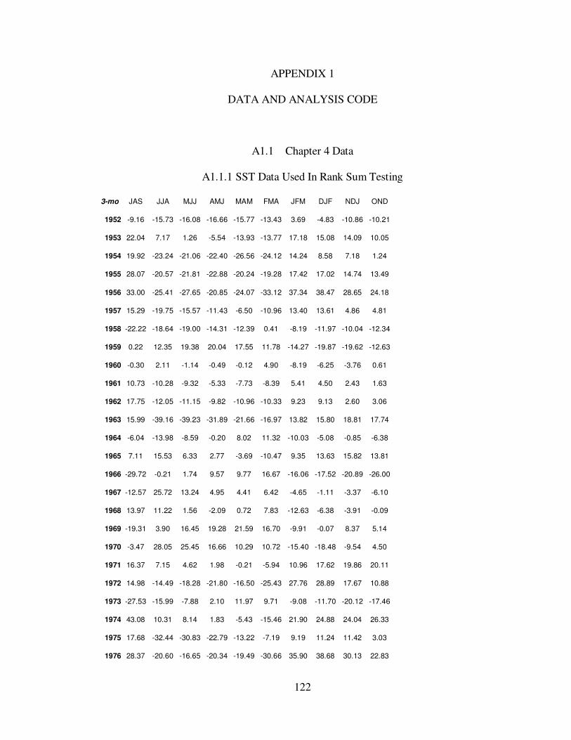
122
APPENDIX 1
DATA AND ANALYSIS CODE
A1.1 Chapter 4 Data
A1.1.1 SST Data Used In Rank Sum Testing
3-mo JAS JJA MJJ AMJ MAM FMA JFM DJF NDJ OND
1952 -9.16 -15.73 -16.08 -16.66 -15.77 -13.43 3.69 -4.83 -10.86 -10.21
1953 22.04 7.17 1.26 -5.54 -13.93 -13.77 17.18 15.08 14.09 10.05
1954 19.92 -23.24 -21.06 -22.40 -26.56 -24.12 14.24 8.58 7.18 1.24
1955 28.07 -20.57 -21.81 -22.88 -20.24 -19.28 17.42 17.02 14.74 13.49
1956 33.00 -25.41 -27.65 -20.85 -24.07 -33.12 37.34 38.47 28.65 24.18
1957 15.29 -19.75 -15.57 -11.43 -6.50 -10.96 13.40 13.61 4.86 4.81
1958 -22.22 -18.64 -19.00 -14.31 -12.39 0.41 -8.19 -11.97 -10.04 -12.34
1959 0.22 12.35 19.38 20.04 17.55 11.78 -14.27 -19.87 -19.62 -12.63
1960 -0.30 2.11 -1.14 -0.49 -0.12 4.90 -8.19 -6.25 -3.76 0.61
1961 10.73 -10.28 -9.32 -5.33 -7.73 -8.39 5.41 4.50 2.43 1.63
1962 17.75 -12.05 -11.15 -9.82 -10.96 -10.33 9.23 9.13 2.60 3.06
1963 15.99 -39.16 -39.23 -31.89 -21.66 -16.97 13.82 15.80 18.81 17.74
1964 -6.04 -13.98 -8.59 -0.20 8.02 11.32 -10.03 -5.08 -0.85 -6.38
1965 7.11 15.53 6.33 2.77 -3.69 -10.47 9.35 13.63 15.82 13.81
1966 -29.72 -0.21 1.74 9.57 9.77 16.67 -16.06 -17.52 -20.89 -26.00
1967 -12.57 25.72 13.24 4.95 4.41 6.42 -4.65 -1.11 -3.37 -6.10
1968 13.97 11.22 1.56 -2.09 0.72 7.83 -12.63 -6.38 -3.91 -0.09
1969 -19.31 3.90 16.45 19.28 21.59 16.70 -9.91 -0.07 8.37 5.14
1970 -3.47 28.05 25.45 16.66 10.29 10.72 -15.40 -18.48 -9.54 4.50
1971 16.37 7.15 4.62 1.98 -0.21 -5.94 10.96 17.62 19.86 20.11
1972 14.98 -14.49 -18.28 -21.80 -16.50 -25.43 27.76 28.89 17.67 10.88
1973 -27.53 -15.99 -7.88 2.10 11.97 9.71 -9.08 -11.70 -20.12 -17.46
1974 43.08 10.31 8.14 1.83 -5.43 -15.46 21.90 24.88 24.04 26.33
1975 17.68 -32.44 -30.83 -22.79 -13.22 -7.19 9.19 11.24 11.42 3.03
1976 28.37 -20.60 -16.65 -20.34 -19.49 -30.66 35.90 38.68 30.13 22.83

123
1977 -14.54 -19.51 -17.51 -14.78 -11.20 -13.69 9.39 -8.92 -16.24 -16.83
1978 -24.44 30.88 31.49 20.01 6.66 1.74 -10.29 -26.63 -30.13 -28.03
1979 -22.34 20.14 20.00 27.03 30.28 25.98 -17.14 -15.63 -17.57 -12.83
1980 -32.83 15.38 10.39 7.41 2.29 11.16 -17.97 -25.44 -27.12 -31.26
1981 -12.27 34.75 38.73 34.19 29.30 25.11 -20.68 -24.57 -22.94 -15.98
1982 -17.05 27.06 25.33 20.55 16.38 12.10 -16.37 -28.25 -36.09 -30.54
1983 -63.02 23.23 22.51 18.90 18.29 16.28 -19.80 -23.72 -28.82 -34.24
1984 -17.14 65.25 64.79 65.31 65.15 64.63 -54.90 -49.18 -47.28 -38.34
1985 -22.22 20.46 24.96 19.68 11.07 4.81 -3.60 -5.03 -10.59 -14.71
1986 -9.04 16.36 11.42 0.19 -4.98 -12.30 6.07 -3.56 -9.66 -12.10
1987 -33.44 -4.86 1.21 5.50 9.34 16.25 -17.81 -22.67 -25.82 -27.74
1988 -16.77 16.58 17.79 18.76 20.79 26.31 -26.28 -22.49 -18.44 -13.80
1989 32.54 2.55 -9.19 -12.09 -11.74 -8.61 14.20 22.41 26.48 28.96
1990 8.37 -26.80 -28.47 -27.37 -15.17 -7.93 7.80 7.31 8.42 13.94
1991 6.22 1.55 4.93 1.24 0.92 5.72 -11.15 -7.10 -1.30 -0.45
1992 -23.73 -0.17 9.04 12.60 4.79 -0.67 7.77 7.49 12.16 2.27
1993 -23.80 31.33 31.36 33.32 41.22 54.54 -55.03 -47.37 -35.20 -31.93
1994 -21.25 21.31 23.52 30.84 30.24 32.29 -32.45 -21.25 -11.90 -5.18
1995 -24.40 17.20 12.62 12.19 13.05 15.59 -20.67 -18.91 -20.37 -20.47
1996 17.09 19.07 16.62 24.19 24.71 20.21 -9.54 -10.11 4.82 10.76
1997 -10.77 0.10 11.50 12.74 10.60 17.68 -15.62 -9.91 5.08 2.80
1998 -34.13 8.77 6.93 5.75 7.06 20.10 -35.92 -35.93 -29.91 -28.76
1999 53.00 27.03 25.08 32.07 29.53 15.58 1.81 13.24 21.60 29.81
2000 55.24 -62.67 -61.68 -64.84 -62.89 -69.88 69.87 69.00 63.00 60.10
2001 32.00 -55.50 -54.24 -50.52 -48.03 -48.54 49.64 50.65 44.05 34.38
2002 41.96 -30.99 -27.57 -31.51 -35.96 -41.09 48.51 51.57 51.16 45.49
2003 -3.50 -44.83 -50.89 -53.25 -48.09 -29.71 22.24 20.79 22.40 21.77
2004 6.00 5.34 5.38 1.51 0.55 -4.63 9.53 10.31 12.49 20.69
6-mo AMJJAS MAMJJA FMAMJJ JFMAMJ DJFMAM NDJFMA ONDJFM
1952 -18.49 -17.32 -17.86 -13.95 -11.04 -3.88 -4.30
1953 4.04 -1.43 -6.22 -11.54 -14.70 -15.79 15.47
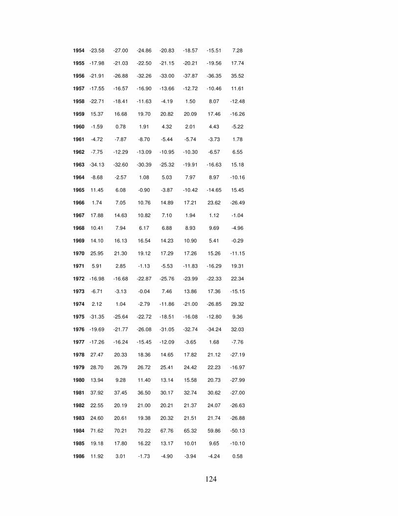
124
1954 -23.58 -27.00 -24.86 -20.83 -18.57 -15.51 7.28
1955 -17.98 -21.03 -22.50 -21.15 -20.21 -19.56 17.74
1956 -21.91 -26.88 -32.26 -33.00 -37.87 -36.35 35.52
1957 -17.55 -16.57 -16.90 -13.66 -12.72 -10.46 11.61
1958 -22.71 -18.41 -11.63 -4.19 1.50 8.07 -12.48
1959 15.37 16.68 19.70 20.82 20.09 17.46 -16.26
1960 -1.59 0.78 1.91 4.32 2.01 4.43 -5.22
1961 -4.72 -7.87 -8.70 -5.44 -5.74 -3.73 1.78
1962 -7.75 -12.29 -13.09 -10.95 -10.30 -6.57 6.55
1963 -34.13 -32.60 -30.39 -25.32 -19.91 -16.63 15.18
1964 -8.68 -2.57 1.08 5.03 7.97 8.97 -10.16
1965 11.45 6.08 -0.90 -3.87 -10.42 -14.65 15.45
1966 1.74 7.05 10.76 14.89 17.21 23.62 -26.49
1967 17.88 14.63 10.82 7.10 1.94 1.12 -1.04
1968 10.41 7.94 6.17 6.88 8.93 9.69 -4.96
1969 14.10 16.13 16.54 14.23 10.90 5.41 -0.29
1970 25.95 21.30 19.12 17.29 17.26 15.26 -11.15
1971 5.91 2.85 -1.13 -5.53 -11.83 -16.29 19.31
1972 -16.98 -16.68 -22.87 -25.76 -23.99 -22.33 22.34
1973 -6.71 -3.13 -0.04 7.46 13.86 17.36 -15.15
1974 2.12 1.04 -2.79 -11.86 -21.00 -26.85 29.32
1975 -31.35 -25.64 -22.72 -18.51 -16.08 -12.80 9.36
1976 -19.69 -21.77 -26.08 -31.05 -32.74 -34.24 32.03
1977 -17.26 -16.24 -15.45 -12.09 -3.65 1.68 -7.76
1978 27.47 20.33 18.36 14.65 17.82 21.12 -27.19
1979 28.70 26.79 26.72 25.41 24.42 22.23 -16.97
1980 13.94 9.28 11.40 13.14 15.58 20.73 -27.99
1981 37.92 37.45 36.50 30.17 32.74 30.62 -27.00
1982 22.55 20.19 21.00 20.21 21.37 24.07 -26.63
1983 24.60 20.61 19.38 20.32 21.51 21.74 -26.88
1984 71.62 70.21 70.22 67.76 65.32 59.86 -50.13
1985 19.18 17.80 16.22 13.17 10.01 9.65 -10.10
1986 11.92 3.01 -1.73 -4.90 -3.94 -4.24 0.58
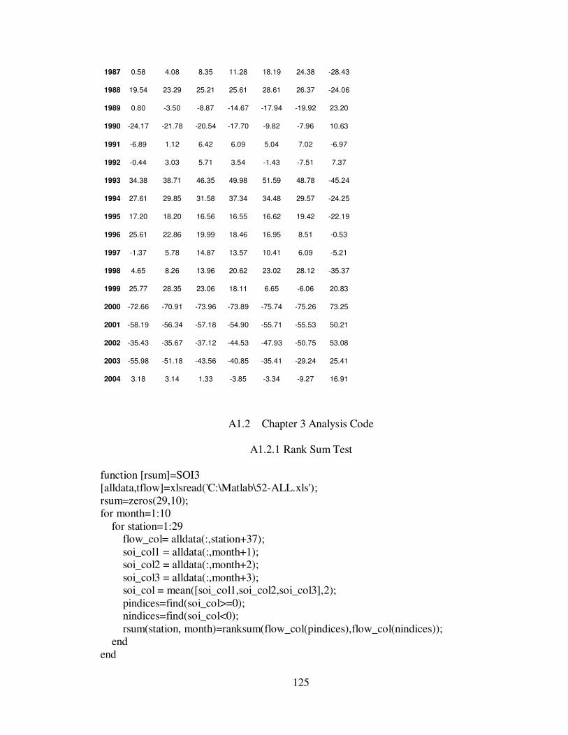
125
1987 0.58 4.08 8.35 11.28 18.19 24.38 -28.43
1988 19.54 23.29 25.21 25.61 28.61 26.37 -24.06
1989 0.80 -3.50 -8.87 -14.67 -17.94 -19.92 23.20
1990 -24.17 -21.78 -20.54 -17.70 -9.82 -7.96 10.63
1991 -6.89 1.12 6.42 6.09 5.04 7.02 -6.97
1992 -0.44 3.03 5.71 3.54 -1.43 -7.51 7.37
1993 34.38 38.71 46.35 49.98 51.59 48.78 -45.24
1994 27.61 29.85 31.58 37.34 34.48 29.57 -24.25
1995 17.20 18.20 16.56 16.55 16.62 19.42 -22.19
1996 25.61 22.86 19.99 18.46 16.95 8.51 -0.53
1997 -1.37 5.78 14.87 13.57 10.41 6.09 -5.21
1998 4.65 8.26 13.96 20.62 23.02 28.12 -35.37
1999 25.77 28.35 23.06 18.11 6.65 -6.06 20.83
2000 -72.66 -70.91 -73.96 -73.89 -75.74 -75.26 73.25
2001 -58.19 -56.34 -57.18 -54.90 -55.71 -55.53 50.21
2002 -35.43 -35.67 -37.12 -44.53 -47.93 -50.75 53.08
2003 -55.98 -51.18 -43.56 -40.85 -35.41 -29.24 25.41
2004 3.18 3.14 1.33 -3.85 -3.34 -9.27 16.91
A1.2 Chapter 3 Analysis Code
A1.2.1 Rank Sum Test
function [rsum]=SOI3 [alldata,tflow]=xlsread('C:\Matlab\52-ALL.xls'); rsum=zeros(29,10); for month=1:10 for station=1:29 flow_col= alldata(:,station+37); soi_col1 = alldata(:,month+1); soi_col2 = alldata(:,month+2); soi_col3 = alldata(:,month+3); soi_col = mean([soi_col1,soi_col2,soi_col3],2); pindices=find(soi_col>=0); nindices=find(soi_col<0); rsum(station, month)=ranksum(flow_col(pindices),flow_col(nindices)); end end

126
function [rsum]=SOI6 [alldata,tflow]=xlsread('C:\Matlab\52-ALL.xls'); rsum=zeros(29,7); for month=1:7 for station=1:29 flow_col= alldata(:,station+37); soi_col1 = alldata(:,month+1); soi_col2 = alldata(:,month+2); soi_col3 = alldata(:,month+3); soi_col4 = alldata(:,month+4); soi_col5 = alldata(:,month+5); soi_col6 = alldata(:,month+6); soi_col = mean([soi_col1,soi_col2,soi_col3,soi_col4,soi_col5,soi_col6],2); pindices=find(soi_col>=0); nindices=find(soi_col<0); rsum(station, month)=ranksum(flow_col(pindices),flow_col(nindices)); end end function [rsum]=PDO3 [alldata,tflow]=xlsread('C:\Matlab\52-ALL.xls'); rsum=zeros(29,10); for month=1:10 for station=1:29 flow_col= alldata(:,station+37); pdo_col1 = alldata(:,month+25); pdo_col2 = alldata(:,month+26); pdo_col3 = alldata(:,month+27); pdo_col = mean([pdo_col1,pdo_col2,pdo_col3],2); pindices=find(pdo_col>=0); nindices=find(pdo_col<0); rsum(station, month)=ranksum(flow_col(pindices),flow_col(nindices)); end end function [rsum]=PDO6 [alldata,tflow]=xlsread('C:\Matlab\52-ALL.xls'); rsum=zeros(29,7); for month=1:7 for station=1:29 flow_col= alldata(:,station+37); pdo_col1 = alldata(:,month+25); pdo_col2 = alldata(:,month+26); pdo_col3 = alldata(:,month+27); pdo_col4 = alldata(:,month+28); pdo_col5 = alldata(:,month+29);
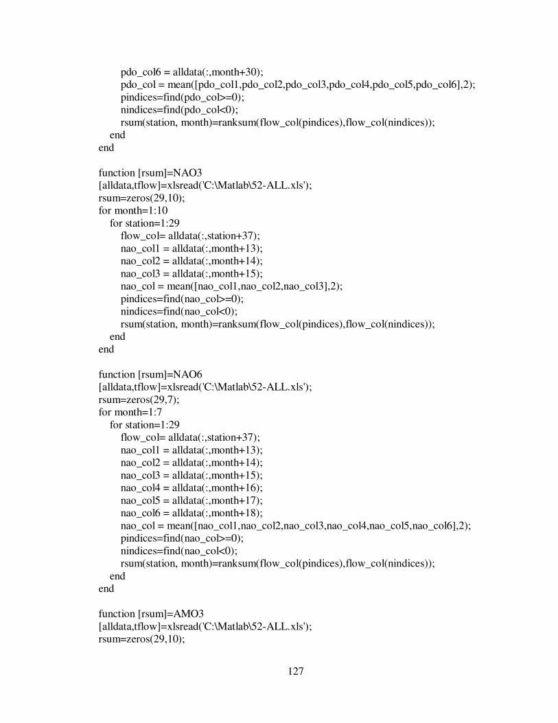
127
pdo_col6 = alldata(:,month+30); pdo_col = mean([pdo_col1,pdo_col2,pdo_col3,pdo_col4,pdo_col5,pdo_col6],2); pindices=find(pdo_col>=0); nindices=find(pdo_col<0); rsum(station, month)=ranksum(flow_col(pindices),flow_col(nindices)); end end function [rsum]=NAO3 [alldata,tflow]=xlsread('C:\Matlab\52-ALL.xls'); rsum=zeros(29,10); for month=1:10 for station=1:29 flow_col= alldata(:,station+37); nao_col1 = alldata(:,month+13); nao_col2 = alldata(:,month+14); nao_col3 = alldata(:,month+15); nao_col = mean([nao_col1,nao_col2,nao_col3],2); pindices=find(nao_col>=0); nindices=find(nao_col<0); rsum(station, month)=ranksum(flow_col(pindices),flow_col(nindices)); end end function [rsum]=NAO6 [alldata,tflow]=xlsread('C:\Matlab\52-ALL.xls'); rsum=zeros(29,7); for month=1:7 for station=1:29 flow_col= alldata(:,station+37); nao_col1 = alldata(:,month+13); nao_col2 = alldata(:,month+14); nao_col3 = alldata(:,month+15); nao_col4 = alldata(:,month+16); nao_col5 = alldata(:,month+17); nao_col6 = alldata(:,month+18); nao_col = mean([nao_col1,nao_col2,nao_col3,nao_col4,nao_col5,nao_col6],2); pindices=find(nao_col>=0); nindices=find(nao_col<0); rsum(station, month)=ranksum(flow_col(pindices),flow_col(nindices)); end end function [rsum]=AMO3 [alldata,tflow]=xlsread('C:\Matlab\52-ALL.xls'); rsum=zeros(29,10);
128
for month=1:10 for station=1:29 flow_col= alldata(:,station+37); amo_col1 = alldata(:,month+66); amo_col2 = alldata(:,month+67); amo_col3 = alldata(:,month+68); amo_col = mean([amo_col1,amo_col2,amo_col3],2); pindices=find(amo_col>=0); nindices=find(amo_col<0); rsum(station, month)=ranksum(flow_col(pindices),flow_col(nindices)); end end function [rsum]=AMO6 [alldata,tflow]=xlsread('C:\Matlab\52-ALL.xls'); rsum=zeros(29,7); for month=1:7 for station=1:29 flow_col= alldata(:,station+37); amo_col1 = alldata(:,month+66); amo_col2 = alldata(:,month+67); amo_col3 = alldata(:,month+68); amo_col4 = alldata(:,month+69); amo_col5 = alldata(:,month+70); amo_col6 = alldata(:,month+71); amo_col = mean([amo_col1,amo_col2,amo_col3,amo_col4,amo_col5,amo_col6],2); pindices=find(amo_col>=0); nindices=find(amo_col<0); rsum(station, month)=ranksum(flow_col(pindices),flow_col(nindices)); end end function [rsum]=SPb3 [alldata,tflow]=xlsread('C:\Matlab\52-ALL.xls'); % Calculation of the SOI & PDO pos. versus the SOI pos. & PDO neg. rsum=zeros(29,10); for month=1:10 for station=1:29 flow_col= alldata(:,station+37); soi_col1 = alldata(:,month+1); soi_col2 = alldata(:,month+2); soi_col3 = alldata(:,month+3); pdo_col1 = alldata(:,month+25); pdo_col2 = alldata(:,month+26); pdo_col3 = alldata(:,month+27); soi_col = mean([soi_col1,soi_col2,soi_col3],2);

129
pdo_col = mean([pdo_col1,pdo_col2,pdo_col3],2); pindices=find(soi_col>=0 & pdo_col>=0); nindices=find(soi_col>=0 & pdo_col<0); rsum(station, month)=ranksum(flow_col(pindices),flow_col(nindices)); end end function [rsum]=SPb6 [alldata,tflow]=xlsread('C:\Matlab\52-ALL.xls'); % Calculation of the SOI & PDO pos. versus the SOI pos. & PDO neg. rsum=zeros(29,7); for month=1:7 for station=1:29 flow_col= alldata(:,station+37); soi_col1 = alldata(:,month+1); soi_col2 = alldata(:,month+2); soi_col3 = alldata(:,month+3); soi_col4 = alldata(:,month+4); soi_col5 = alldata(:,month+5); soi_col6 = alldata(:,month+6); pdo_col1 = alldata(:,month+25); pdo_col2 = alldata(:,month+26); pdo_col3 = alldata(:,month+27); pdo_col4 = alldata(:,month+28); pdo_col5 = alldata(:,month+29); pdo_col6 = alldata(:,month+30); soi_col = mean([soi_col1,soi_col2,soi_col3,soi_col4,soi_col5,soi_col6],2); pdo_col = mean([pdo_col1,pdo_col2,pdo_col3,pdo_col4,pdo_col5,pdo_col6],2); pindices=find(soi_col>=0 & pdo_col>=0); nindices=find(soi_col>=0 & pdo_col<0); rsum(station, month)=ranksum(flow_col(pindices),flow_col(nindices)); end end function [rsum]=SPd3 [alldata,tflow]=xlsread('C:\Matlab\52-ALL.xls'); % Calculation of the SOI & PDO neg. versus the SOI neg. & PDO pos. rsum=zeros(29,10); for month=1:10 for station=1:29 flow_col= alldata(:,station+37); soi_col1 = alldata(:,month+1); soi_col2 = alldata(:,month+2); soi_col3 = alldata(:,month+3); pdo_col1 = alldata(:,month+25); pdo_col2 = alldata(:,month+26);
130
pdo_col3 = alldata(:,month+27); soi_col = mean([soi_col1,soi_col2,soi_col3],2); pdo_col = mean([pdo_col1,pdo_col2,pdo_col3],2); pindices=find(soi_col<0 & pdo_col<0); nindices=find(soi_col<0 & pdo_col>=0); rsum(station, month)=ranksum(flow_col(pindices),flow_col(nindices)); end end function [rsum]=SPd6 [alldata,tflow]=xlsread('C:\Matlab\52-ALL.xls'); % Calculation of the SOI & PDO neg. versus the SOI neg. & PDO pos. rsum=zeros(29,7); for month=1:7 for station=1:29 flow_col= alldata(:,station+37); soi_col1 = alldata(:,month+1); soi_col2 = alldata(:,month+2); soi_col3 = alldata(:,month+3); soi_col4 = alldata(:,month+4); soi_col5 = alldata(:,month+5); soi_col6 = alldata(:,month+6); pdo_col1 = alldata(:,month+25); pdo_col2 = alldata(:,month+26); pdo_col3 = alldata(:,month+27); pdo_col4 = alldata(:,month+28); pdo_col5 = alldata(:,month+29); pdo_col6 = alldata(:,month+30); soi_col = mean([soi_col1,soi_col2,soi_col3,soi_col4,soi_col5,soi_col6],2); pdo_col = mean([pdo_col1,pdo_col2,pdo_col3,pdo_col4,pdo_col5,pdo_col6],2); pindices=find(soi_col<0 & pdo_col<0); nindices=find(soi_col<0 & pdo_col>=0); rsum(station, month)=ranksum(flow_col(pindices),flow_col(nindices)); end end function [rsum]=SNb3 [alldata,tflow]=xlsread('C:\Matlab\52-ALL.xls'); % Calculation of the SOI & NAO pos. versus the SOI pos. & NAO neg. rsum=zeros(29,10); for month=1:10 for station=1:29 flow_col= alldata(:,station+37); soi_col1 = alldata(:,month+1); soi_col2 = alldata(:,month+2); soi_col3 = alldata(:,month+3);

131
nao_col1 = alldata(:,month+13); nao_col2 = alldata(:,month+14); nao_col3 = alldata(:,month+15); soi_col = mean([soi_col1,soi_col2,soi_col3],2); nao_col = mean([nao_col1,nao_col2,nao_col3],2); pindices=find(soi_col>=0 & nao_col>=0); nindices=find(soi_col>=0 & nao_col<0); rsum(station, month)=ranksum(flow_col(pindices),flow_col(nindices)); end end function [rsum]=SNb6 [alldata,tflow]=xlsread('C:\Matlab\52-ALL.xls'); % Calculation of the SOI & NAO pos. versus the SOI pos. & NAO neg. rsum=zeros(29,7); for month=1:7 for station=1:29 flow_col= alldata(:,station+37); soi_col1 = alldata(:,month+1); soi_col2 = alldata(:,month+2); soi_col3 = alldata(:,month+3); soi_col4 = alldata(:,month+4); soi_col5 = alldata(:,month+5); soi_col6 = alldata(:,month+6); nao_col1 = alldata(:,month+13); nao_col2 = alldata(:,month+14); nao_col3 = alldata(:,month+15); nao_col4 = alldata(:,month+16); nao_col5 = alldata(:,month+17); nao_col6 = alldata(:,month+18); soi_col = mean([soi_col1,soi_col2,soi_col3,soi_col4,soi_col5,soi_col6],2); nao_col = mean([nao_col1,nao_col2,nao_col3,nao_col4,nao_col5,nao_col6],2); pindices=find(soi_col>=0 & nao_col>=0); nindices=find(soi_col>=0 & nao_col<0); rsum(station, month)=ranksum(flow_col(pindices),flow_col(nindices)); end end function [rsum]=SNd3 [alldata,tflow]=xlsread('C:\Matlab\52-ALL.xls'); % Calculation of the SOI & nao neg. versus the SOI neg. & nao pos. rsum=zeros(29,10); for month=1:10 for station=1:29 flow_col= alldata(:,station+37); soi_col1 = alldata(:,month+1);
132
soi_col2 = alldata(:,month+2); soi_col3 = alldata(:,month+3); nao_col1 = alldata(:,month+13); nao_col2 = alldata(:,month+14); nao_col3 = alldata(:,month+15); soi_col = mean([soi_col1,soi_col2,soi_col3],2); nao_col = mean([nao_col1,nao_col2,nao_col3],2); pindices=find(soi_col<0 & nao_col<0); nindices=find(soi_col<0 & nao_col>=0); rsum(station, month)=ranksum(flow_col(pindices),flow_col(nindices)); end end function [rsum]=SNd6 [alldata,tflow]=xlsread('C:\Matlab\52-ALL.xls'); % Calculation of the SOI & nao neg. versus the SOI neg. & nao pos. rsum=zeros(29,7); for month=1:7 for station=1:29 flow_col= alldata(:,station+37); soi_col1 = alldata(:,month+1); soi_col2 = alldata(:,month+2); soi_col3 = alldata(:,month+3); soi_col4 = alldata(:,month+4); soi_col5 = alldata(:,month+5); soi_col6 = alldata(:,month+6); nao_col1 = alldata(:,month+13); nao_col2 = alldata(:,month+14); nao_col3 = alldata(:,month+15); nao_col4 = alldata(:,month+16); nao_col5 = alldata(:,month+17); nao_col6 = alldata(:,month+18); soi_col = mean([soi_col1,soi_col2,soi_col3,soi_col4,soi_col5,soi_col6],2); nao_col = mean([nao_col1,nao_col2,nao_col3,nao_col4,nao_col5,nao_col6],2); pindices=find(soi_col<0 & nao_col<0); nindices=find(soi_col<0 & nao_col>=0); rsum(station, month)=ranksum(flow_col(pindices),flow_col(nindices)); end end function [rsum]=SAb3 [alldata,tflow]=xlsread('C:\Matlab\52-ALL.xls'); % Calculation of the SOI & AMO pos. versus the SOI pos. & AMO neg. rsum=zeros(29,10); for month=1:10 for station=1:29

133
flow_col= alldata(:,station+37); soi_col1 = alldata(:,month+1); soi_col2 = alldata(:,month+2); soi_col3 = alldata(:,month+3); amo_col1 = alldata(:,month+66); amo_col2 = alldata(:,month+67); amo_col3 = alldata(:,month+68); soi_col = mean([soi_col1,soi_col2,soi_col3],2); amo_col = mean([amo_col1,amo_col2,amo_col3],2); pindices=find(soi_col>=0 & amo_col>=0); nindices=find(soi_col>=0 & amo_col<0); rsum(station, month)=ranksum(flow_col(pindices),flow_col(nindices)); end end function [rsum]=SAb6 [alldata,tflow]=xlsread('C:\Matlab\52-ALL.xls'); % Calculation of the SOI & AMO pos. versus the SOI pos. & AMO neg. rsum=zeros(29,7); for month=1:7 for station=1:29 flow_col= alldata(:,station+37); soi_col1 = alldata(:,month+1); soi_col2 = alldata(:,month+2); soi_col3 = alldata(:,month+3); soi_col4 = alldata(:,month+4); soi_col5 = alldata(:,month+5); soi_col6 = alldata(:,month+6); amo_col1 = alldata(:,month+66); amo_col2 = alldata(:,month+67); amo_col3 = alldata(:,month+68); amo_col4 = alldata(:,month+69); amo_col5 = alldata(:,month+70); amo_col6 = alldata(:,month+71); soi_col = mean([soi_col1,soi_col2,soi_col3,soi_col4,soi_col5,soi_col6],2); amo_col = mean([amo_col1,amo_col2,amo_col3,amo_col4,amo_col5,amo_col6],2); pindices=find(soi_col>=0 & amo_col>=0); nindices=find(soi_col>=0 & amo_col<0); rsum(station, month)=ranksum(flow_col(pindices),flow_col(nindices)); end end function [rsum]=SAd3 [alldata,tflow]=xlsread('C:\Matlab\52-ALL.xls'); % Calculation of the SOI & AMO neg. versus the SOI neg. & AMO pos. rsum=zeros(29,10);

134
for month=1:10 for station=1:29 flow_col= alldata(:,station+37); soi_col1 = alldata(:,month+1); soi_col2 = alldata(:,month+2); soi_col3 = alldata(:,month+3); amo_col1 = alldata(:,month+66); amo_col2 = alldata(:,month+67); amo_col3 = alldata(:,month+68); soi_col = mean([soi_col1,soi_col2,soi_col3],2); amo_col = mean([amo_col1,amo_col2,amo_col3],2); pindices=find(soi_col<0 & amo_col<0); nindices=find(soi_col<0 & amo_col>=0); rsum(station, month)=ranksum(flow_col(pindices),flow_col(nindices)); end end function [rsum]=SAd6 [alldata,tflow]=xlsread('C:\Matlab\52-ALL.xls'); % Calculation of the SOI & AMO neg. versus the SOI neg. & AMO pos. rsum=zeros(29,7); for month=1:7 for station=1:29 flow_col= alldata(:,station+37); soi_col1 = alldata(:,month+1); soi_col2 = alldata(:,month+2); soi_col3 = alldata(:,month+3); soi_col4 = alldata(:,month+4); soi_col5 = alldata(:,month+5); soi_col6 = alldata(:,month+6); amo_col1 = alldata(:,month+66); amo_col2 = alldata(:,month+67); amo_col3 = alldata(:,month+68); amo_col4 = alldata(:,month+69); amo_col5 = alldata(:,month+70); amo_col6 = alldata(:,month+71); soi_col = mean([soi_col1,soi_col2,soi_col3,soi_col4,soi_col5,soi_col6],2); amo_col = mean([amo_col1,amo_col2,amo_col3,amo_col4,amo_col5,amo_col6],2); pindices=find(soi_col<0 & amo_col<0); nindices=find(soi_col<0 & amo_col>=0); rsum(station, month)=ranksum(flow_col(pindices),flow_col(nindices)); end end function [rsum]=SST3 [alldata]=xlsread('C:\Matlab\52-ALL.xls');

135
rsum=zeros(29,10); for month=1:10 for station=1:29 flow_col = alldata(:,station+37); sst3_col = alldata(:,month+78); pindices=find(sst3_col>=0); nindices=find(sst3_col<0); rsum(station, month)=ranksum(flow_col(pindices),flow_col(nindices)); end end function [rsum]=SST6 [alldata,tflow]=xlsread('C:\Matlab\52-ALL.xls'); rsum=zeros(29,7); for month=1:7 for station=1:29 flow_col = alldata(:,station+37); sst6_col = alldata(:,month+88); pindices=find(sst6_col>=0); nindices=find(sst6_col<0); rsum(station, month)=ranksum(flow_col(pindices),flow_col(nindices)); end end
A1.2.2 SVD Analysis And Mapping
%---------------------------------------------------------------------------------------- %Code reads in SST data and then removes the -9999 values which denote land temps = xlsread('C:\Matlab\SVD\SST-RAW.xls'); temps = temps(3:end,4:56); m = 0; for i = -70:2:70; % Latitude for j = 120:2:280; % Longitude m = m +1; b(m,:) = [i j]; end end remv_rows = find(temps(:,1) == -9999); %all_temps(remv_rows,:) = []; temps(remv_rows,:) = []; b(remv_rows,:) = [];

136
all_temps = [b temps]; col = size(temps,2); % Take row average, by adding the ',2' inside the parenthesis. round1 = mean(temps,2); %Standardize each row (hence the ',2' term again). The middle term % (e.g. '0') tells the function to use n-1 when standardizing. round1st = std(temps,0,2); for i = 1:col round2(:,i) = temps(:,i) - round1; % Substruct each row element to row mean end round2mn = mean(round2,2); round2st = std(round2,0,2); % Get standard deviation for j = 1:col round3(:,j) = (round2(:,j)- round2mn)./round2st; % Standardize end m round3(isnan(round3))=0; xlswrite('C:\MATLAB\SVD\SST_lat_long.xls',b); % Write to excel file xlswrite('C:\MATLAB\SVD\std_sst.xls',roun3); %--------------------------------------------------------------------------------------------- % Runs SVD and calculates the correlation values from the SVD results. % Create a Matlab directory in C % C:\Matlab % Or use a different directory. However lines 37 52 53 115-118 % needs to be changed accordingly % Other parameters that can be changed on lines... % Lines 12, 13, 146, 147, 219, 220 clc clear temp1 = xlsread('C:\matlab\SVD95\SVD-0-JAS\Std_SST.xls'); %import standardized ssts. str1 = xlsread('C:\matlab\std-streamflow.xls'); %inport standardized sst [stations years] = size(str1); %input('Enter the number of years: '); t = temp1'; s = str1';

137
%calculating covariance covar_ts = (1/years) * t' * s; % svd calculation [left, eigs, right] = svd(covar_ts); % Get the number of modes by calculating % the square covariance and check for values >10 eigenvalues = diag(eigs); square_eig = eigenvalues.^2; %squares of the values sum_sq_eig = sum(square_eig) ; %sum of the squares square_cov = square_eig./sum_sq_eig; %square covariance sign_num = find(square_cov >= 0.11); %find values greater than 10% sign_num_val = square_cov(sign_num); num_modes = numel(sign_num); %How many values greater than 10% % Export square covariance data to an excel file xlswrite('C:\matlab\SVD95\SVD-0-JAS\square_covar.xls',square_cov); % Getting temporal expansion for i = 1:num_modes; %num_modes; a = left(:,i); left_exp = t*a; %Create a matrix of left left_exp_mat(:,i) = left_exp; %left temporal expansions b = right(:,i); right_exp = s*b; %create a matrix of right right_exp_mat(:,i) = right_exp; %right temporal expansions end % Export temporal expansions matrices to excel files xlswrite('C:\matlab\SVD95\SVD-0-JAS\right_temp_expan.xls',right_exp_mat); xlswrite('C:\matlab\SVD95\SVD-0-JAS\left_temp_expan.xls',left_exp_mat); % Getting Left heterogenous correlation sign_p = input('Significance (in decimal, eg 0.95 for 95%): '); sign_p = 1 - sign_p; [rrt cct] = size(t); [rrs ccs] = size(s); for n = 1:num_modes; rht = right_exp_mat(:,n);

138
for m = 1:cct; left_heter = [t(:,m) rht]; % left heterogenous correlations figure [r,p] = corrcoef(left_heter); %Compute sample correlation and p-values. [k,l] = find(p<sign_p); % Find significant correlations. pp = [k,l]; % Display their (row,col) indices. if isempty(pp) rl = 0; else rl = r(1,2); end bbb(n,m) = rl; r = r(1,2); all_left(n,m) = r; end end left_corr_values = bbb'; all_left_correl = all_left'; %Getting Right heterogeneous correlation for u = 1:num_modes; lht = left_exp_mat(:,u); for v = 1:ccs; right_heter = [s(:,v) lht]; % right heterogenous correlations figure [rr,pr] = corrcoef(right_heter); %Compute sample correlation and p-values. [kr,lr] = find(pr<sign_p); % Find significant correlations. ppr = [kr,lr]; % Display their (row,col) indices. if isempty(ppr) rrs = 0; else rrs = rr(1,2); end bbbr(u,v) = rrs; rr = rr(1,2); corr_valz(u,v) = rr; end end

139
right_corr_values = bbbr'; all_corr_valz = corr_valz'; %Export significant correlation values to excel files xlswrite('C:\matlab\SVD95\SVD-0-JAS\stream_correl.xls',right_corr_values); xlswrite('C:\matlab\SVD95\SVD-0-JAS\SST_correl.xls',left_corr_values); xlswrite('C:\matlab\SVD95\SVD-0-JAS\all_stream_correl.xls',all_corr_valz); xlswrite('C:\matlab\SVD95\SVD-0-JAS\all_sst_correl.xls',all_left_correl); % Information to display num_mode_val = 100.* sign_num_val'; mode_total = sum(num_mode_val); num_m_val = [num_modes mode_total]; fprintf('There are %3.0f modes for this analysis and account for %3.0f percent. \n',num_m_val) display(['The square covariance fractions over 10% are ' int2str(num_mode_val) ' percent.']) disp(' ') %MAPPING SECTION %BELOW MAPPING SECTION. looper = 1; while looper == 1; % Loop to view figures of different modes. % Select what to view, Contour of SST or Streamflow Correlations graph2view = input('Which view do you want(sst = 1 or runoff = 2)? '); if graph2view == 2 nm = input('Enter the mode to view: '); str_latlong = xlsread('C:\matlab\stream_lat_long.xls');%Stream Gauge latitude and longitude snlat = str_latlong(:,1); %xlsread('LatQ.xls'); % snlong = str_latlong(:,2); %xlsread('LongQ.xls'); % latlim = [ 25 50]; % Latitude map limits lonlim = [-125 -100]; % longitude map limits figure ax = usamap(latlim,lonlim); axis off states = shaperead('usastatehi',... 'UseGeoCoords', true, 'BoundingBox', [lonlim', latlim']); faceColors = makesymbolspec('Polygon',... {'INDEX', [1 numel(states)], ... 'FaceColor', white(numel(states))}); %polcmap will assign random colors for states
140
geoshow(ax, states , 'SymbolSpec',faceColors) snvalues = right_corr_values; array1 = [snlat snlong snvalues(:,nm)]; [rows colms]=size(array1); for i = 1:rows; if array1(i,3)>0 snotlats = array1(i,1); snotlongs = array1(i,2); plotm(snotlats,snotlongs,'r.') elseif array1(i,3)<0 snotlats = array1(i,1); snotlongs = array1(i,2); plotm(snotlats,snotlongs,'b.') else snotlats = array1(i,1); snotlongs = array1(i,2); plotm(snotlats,snotlongs,'k.') end end for k = 1:numel(states) labelPointIsWithinLimits =... latlim(1) < states(k).LabelLat &&... latlim(2) > states(k).LabelLat &&... lonlim(1) < states(k).LabelLon &&... lonlim(2) > states(k).LabelLon; if labelPointIsWithinLimits textm(states(k).LabelLat,... states(k).LabelLon, states(k).Name, 'HorizontalAlignment', 'center') end end % SSTs contour Mapping elseif graph2view ==1 %contours % Load the data and extract the (x,y,z) information: lat_long = xlsread('C:\Matlab\SVD95\SVD-0-JAS\SST_lat_long.xls'); % SST latitude and longitude x = lat_long(:,2); %x = xlsread('Lon.xls'); % y = lat_long(:,1); %y = xlsread('Lat.xls'); % % % nn = input('Enter the mode to view: ');

141
z = all_left_correl(:,nn); % Determine the minimum and the maximum x and y values: xmin = min(x); ymin = min(y); xmax = max(x); ymax = max(y); % Define the resolution of the grid: xres=17; yres=9; % Define the range and spacing of the x- and y-coordinates, % and then fit them into X and Y xv = linspace(xmin, xmax, xres); yv = linspace(ymin, ymax, yres); [Xinterp,Yinterp] = meshgrid(xv,yv); % Calculate Z in the X-Y interpolation space, which is an % evenly spaced grid: [xi,yi,Zinterp] = griddata(x,y,z,Xinterp,Yinterp); load coast latlim = [ -33 65]; % SST area map latitude limit lonlim =[120 -80] ; % SST area map longitude limit figure worldmap(latlim,lonlim); axis off patchm(lat,long, 'k') %plotm patchm [c,h] = contourfm(yi,xi,Zinterp,-0.6:0.2:0.6); contourcmap(0.3,'jet','colorbar','on','location','horizontal') load('MyColormaps','sstmap') set(gcf,'Colormap',sstmap) h1 = clabelm(c,h); else disp('Not an acceptable choice.') end disp(' ') looper = input('Do you want to print another figure? (yes = 1, no = 0)'); end disp(' ') disp('I guess you are done for now...') %------------------------------------------------------------ %array used to define the MyColormaps array called in the mapping section sstmap = [1 1 0; 0 1 1; 0 0 1; 0 0.502 1; 1 1 1; … 1 1 1; 1 0 0; 0.6588 0 0; 0.5922 0 0.2941; 0.502 0 0.502]; save MyColormaps sstmap

142
A1.3 Chapter 4 Analysis Code
A1.3.1 NetCDF Processing Code in Matlab
%Code to read and process the .nc data. addpath('C:\Program Files (x86)\MATLAB\R2009a Student\toolbox\matlab\matlab_netCDF_OPeNDAP') addpath('C:\Program Files (x86)\MATLAB\R2009a Student\toolbox\matlab\mexnc') addpath('C:\Program Files (x86)\MATLAB\R2009a Student\toolbox\matlab\snctools') %Step 1. Read in the NetCDF files by grabbing only the correct %level, Lat, and Lon fields %NOTE: NetCDF files are 0-based (e.g first 'column' index is 0 not 1) %is actually 0, not 1. %------------------------------------------------------------------------- %Manual input region east = 280; west = 120; north = 70; south = -30; %use negative numbers to denote lats below the equator gph_level = 500; uwnd_level = 200; mon_int = 3; %This defines how manth months are going to be averaged %------------------------------------------------------------------------- level = nc_varget('hgt.mon.mean.nc','level'); lat = nc_varget('hgt.mon.mean.nc','lat'); lon = nc_varget('hgt.mon.mean.nc','lon'); glev = find(level(:,1) == gph_level); %Specifies the 500mb level wlev = find(level(:,1) == uwnd_level); %Specifies the 200mb level lat_max = find(lat(:,1) == south); %returns northern most lat value lat_min = find(lat(:,1) == north); %returns southern most lat value lon_max = find(lon(:,1) == east); %returns eastern most lon value lon_min = find(lon(:,1) == west); %returns western most lon value gph = nc_varget('hgt.mon.mean.nc','hgt',[0 glev lat_min lon_min],... [-1 1 (lat_max-lat_min+1) (lon_max-lon_min+1)]); uwnd = nc_varget('uwnd.mon.mean.nc','uwnd',[0 wlev lat_min lon_min],... [-1 1 (lat_max-lat_min+1) (lon_max-lon_min+1)]); slp = nc_varget('slp.mon.mean.nc','slp',[0 lat_min lon_min],...

143
[-1 (lat_max-lat_min+1) (lon_max-lon_min+1)]); % Reorganize the data to make it so that it is a 2D matrix. % Such that: Rows = locations, Columns = Time. p_gph = permute(gph,[2 3 1]); p_uwnd = permute(uwnd,[2 3 1]); p_slp = permute(slp,[2 3 1]); sizeg = size(p_gph); sizeu = size(p_uwnd); sizes = size(p_slp); r_gph = reshape(p_gph,(sizeg(1)*sizeg(2)),sizeg(3)); r_uwnd = reshape(p_uwnd,(sizeu(1)*sizeu(2)),sizeu(3)); r_slp = reshape(p_slp,(sizes(1)*sizes(2)),sizes(3)); a = size(r_gph); b = size(r_uwnd); bb = size(r_slp); %Standardize the values of the HGT and UWND datasets based upon location %(i.e. rows of the 2D array). %formula: std value = (value - mean(row))/std(row); g500 = zeros(a(1),a(2)); for yr = 1:a(2) for loc = 1:a(1) g500(loc,yr) = (r_gph(loc,yr) - mean(r_gph(loc,:)))/std(r_gph(loc,:)); end end u200 = zeros(b(1),b(2)); for yr = 1:b(2) for loc = 1:b(1) u200(loc,yr) = (r_uwnd(loc,yr) - mean(r_uwnd(loc,:)))/std(r_uwnd(loc,:)); end end slp0 = zeros(bb(1),bb(2)); for yr = 1:bb(2) for loc = 1:bb(1) slp0(loc,yr) = (r_slp(loc,yr) - mean(r_slp(loc,:)))/std(r_slp(loc,:)); end end %------------------------------------- %Pre-Analysis Calculations %------------------------------------- %To create lagged HGT and UWND data, similar to the SST data already used, %need to create 3-month average values for each year. The output of this %step should be a single value for each year in the data record.

144
%Create the 3-month average for each year for the HGT data: JFM - OND agph_m = zeros(length(g500),62,10); for yr = 1:62 for mon = 1:10 agph_m(:,yr,mon) = mean(g500(:,12*yr-(12-mon):12*yr-(12-(mon+(mon_int-1)))),2); end end c = size(agph_m); ragph_m = reshape(agph_m,(c(1)*c(2)),c(3)); %Create the 3-month average for each year for the HGT data: NDJ - DJF bgph_m = zeros(length(g500),61,2); for yr = 1:61 for month = 1:2 bgph_m(:,yr,month) = mean(g500(:,12*yr-(12-month):12*yr-(12-(month+(mon_int-1)))),2); end end d = size(bgph_m); na_col = NaN(d(1),1,d(3)); bbgph_m = [na_col bgph_m]; dd = size(bbgph_m); rbgph_m = reshape(bbgph_m,(dd(1)*dd(2)),dd(3)); %Combine two matricies and then resape back into a 3D array such that: %Rows = locations; Columns = years; z = correspnding 3-month interval. comb_g = [ragph_m rbgph_m]; %take the DJF, NDJ, OND, SON, ASO inteval and move them to the front of the %combined matrix so that the final matrix is organized by water year and %not claendar year. comb_g2 = [comb_g(:,8:12) comb_g(:,1:7)]; gph_m = reshape(comb_g2,c(1),c(2),12); save gph_m gph_m %------------------------------------------------------------------------- %Repeat process to get 3-month average for each year for the UWND data %------------------------------------------------------------------------- awnd_m = zeros(length(u200),62,10); for yr = 1:62 for mon = 1:10 awnd_m(:,yr,mon) = mean(u200(:,12*yr-(12-mon):12*yr-(12-(mon+(mon_int-1)))),2); end end e = size(awnd_m); rawnd_m = reshape(awnd_m,(e(1)*e(2)),e(3));
145
%Create the 3-month average for each year for the HGT data: NDJ - DJF bwnd_m = zeros(length(u200),61,2); for yr = 1:61 for month = 1:2 bwnd_m(:,yr,month) = mean(u200(:,12*yr-(12-month):12*yr-(12-(month+(mon_int-1)))),2); end end f = size(bwnd_m); na_col = NaN(f(1),1,f(3)); bbwnd_m = [na_col bwnd_m]; ff = size(bbwnd_m); rbwnd_m = reshape(bbwnd_m,(ff(1)*ff(2)),ff(3)); %Combine two matricies and then resape back into a 3D array such that: %Rows = locations; Columns = years; z = correspnding 3-month interval. comb_w = [rawnd_m rbwnd_m]; %take the DJF, NDJ, OND, SON, ASO inteval and move them to the front of the %combined matrix so that the final matrix is organized by water year and %not claendar year. comb_w2 = [comb_w(:,8:12) comb_w(:,1:7)]; wnd_m = reshape(comb_w2,e(1),e(2),12); save wnd_m wnd_m %------------------------------------------------------------------------- %Repeat process to get 3-month average for each year for the SLP data %------------------------------------------------------------------------- aslp_m = zeros(length(slp0),62,10); for yr = 1:62 for mon = 1:10 aslp_m(:,yr,mon) = mean(slp0(:,12*yr-(12-mon):12*yr-(12-(mon+(mon_int-1)))),2); end end f = size(aslp_m); raslp_m = reshape(aslp_m,(f(1)*f(2)),f(3)); %Create the 3-month average for each year for the SLP data: NDJ - DJF bslp_m = zeros(length(slp0),61,2); for yr = 1:61 for month = 1:2 bslp_m(:,yr,month) = mean(slp0(:,12*yr-(12-month):12*yr-(12-(month+(mon_int-1)))),2);

146
end end g = size(bslp_m); na_col = NaN(g(1),1,g(3)); bbslp_m = [na_col bslp_m]; gg = size(bbslp_m); rbslp_m = reshape(bbslp_m,(gg(1)*gg(2)),gg(3)); %Combine two matricies and then resape back into a 3D array such that: %Rows = locations; Columns = years; z = correspnding 3-month interval. comb_s = [raslp_m rbslp_m]; %take the DJF, NDJ, OND, SON, ASO inteval and move them to the front of the %combined matrix so that the final matrix is organized by water year and %not claendar year. comb_s2 = [comb_s(:,8:12) comb_s(:,1:7)]; slp_m = reshape(comb_s2,f(1),f(2),12); save slp_m slp_m %--------------------------------------------------------------- %Create the Lat - Lon vector to plot the data in the SVD output %--------------------------------------------------------------- x = west:2.5:east; y = south:2.5:north; for lon = 1:length(x); for lat = 1:length(y); y_all(lon,lat) = y(end+1-lat); x_all(lon,lat) = x(lon); end end ry_all = reshape(y_all',numel(y_all),1); rx_all = reshape(x_all',numel(x_all),1); lat_lon = [ry_all rx_all]; save lat_lon lat_lon
A1.3.2 SVD Analysis And Mapping
%import standardized ssts and streamflow. yr = input('Which lag year do you want to analyze? '); lag = input('Which 3-month interval do you want to analyze? ');

147
load std_sst temp1 = std_sst(:,13-yr:66-yr,lag+1); %grabs 54 columns %0 year lag = col13: col66 %JAS interval is std_sst(:, :, 1). load std_stream str1 = std_stream; %This is the std streamflow from 1952 - 2005 (N = 54) [stations years] = size(str1); t = temp1'; s = str1'; %calculating covariance covar_ts = (1/years) * t' * s; % svd calculation [left, eigs, right] = svd(covar_ts); % Get the number of modes by calculating % the square covariance and check for values >10 eigenvalues = diag(eigs); square_eig = eigenvalues.^2; %squares of the values sum_sq_eig = sum(square_eig) ; %sum of the squares square_cov = square_eig./sum_sq_eig; %square covariance sign_num = find(square_cov >= 0.11); %find values greater than 10% sign_num_val = square_cov(sign_num); num_modes = numel(sign_num); %How many values greater than 10% % Export square covariance data to an excel file xlswrite('L:\Kenneth Data\Matlab\Phase3\SVD\square_covar.xls',square_cov, '4'); % Getting temporal expansion for i = 1:num_modes; %num_modes; a = left(:,i); left_exp = t*a; %Create a matrix of left left_exp_mat(:,i) = left_exp; %left temporal expansions b = right(:,i); right_exp = s*b; %create a matrix of right right_exp_mat(:,i) = right_exp; %right temporal expansions end % Export temporal expansions matrices to excel files xlswrite('L:\Kenneth Data\matlab\Phase3\SVD\rte.xls',right_exp_mat, '4'); xlswrite('L:\Kenneth Data\matlab\Phase3\SVD\lte.xls',left_exp_mat, '4');

148
% Getting Left heterogenous correlation %sign_p = input('Significance (in decimal, eg 0.95 for 95%): '); sign_p = 1 - 0.95; %To reinstate teh use of the input command, simply replace the 0.95 with %'sign_p', and remove the comment from the previous command. [rrt cct] = size(t); [rrs ccs] = size(s); for n = 1:num_modes; rht = right_exp_mat(:,n); for m = 1:cct; left_heter = [t(:,m) rht]; % left heterogenous correlations figure [r,p] = corrcoef(left_heter); %Compute sample correlation and p-values. [k,l] = find(p<sign_p); % Find significant correlations. pp = [k,l]; % Display their (row,col) indices. if isempty(pp) rl = 0; else rl = r(1,2); end bbb(n,m) = rl; r = r(1,2); all_left(n,m) = r; end end left_corr_values = bbb'; all_left_correl = all_left'; %Getting Right heterogeneous correlation for u = 1:num_modes; lht = left_exp_mat(:,u); for v = 1:ccs; right_heter = [s(:,v) lht]; % right heterogenous correlations figure [rr,pr] = corrcoef(right_heter); %Compute sample correlation and p-values.

149
[kr,lr] = find(pr<sign_p); % Find significant correlations. ppr = [kr,lr]; % Display their (row,col) indices. if isempty(ppr) rrs = 0; else rrs = rr(1,2); end bbbr(u,v) = rrs; rr = rr(1,2); corr_valz(u,v) = rr; end end right_corr_values = bbbr'; all_corr_valz = corr_valz'; %Export significant correlation values to excel files xlswrite('L:\Kenneth Data\matlab\Phase3\SVD\stream_correl.xls',right_corr_values, '4'); xlswrite('L:\Kenneth Data\matlab\Phase3\SVD\SST_correl.xls',left_corr_values, '4'); xlswrite('L:\Kenneth Data\matlab\Phase3\SVD\all_stream_correl.xls',all_corr_valz, '4'); xlswrite('L:\Kenneth Data\matlab\Phase3\SVD\all_sst_correl.xls',all_left_correl, '4'); % Information to display %num_mode_val = 100.* sign_num_val'; %mode_total = sum(num_mode_val); %num_m_val = [num_modes mode_total]; %fprintf('There are %3.0f modes for this analysis and account for %3.0f percent. \n',num_m_val) %display(['The square covariance fractions over 10% are ' int2str(num_mode_val) ' percent.']) %disp(' ') %MAPPING SECTION %BELOW MAPPING SECTION. looper = 1; while looper == 1; % Loop to view figures of different modes. % Select what to view, Contour of SST or Streamflow Correlations

150
graph2view = input('Which view do you want(sst = 1 or runoff = 2)? '); if graph2view == 2 nm = input('Enter the mode to view: '); str_latlong = xlsread('L:\Kenneth Data\matlab\PhaseX\stream_lat_long.xls');%Stream Gauge latitude and longitude snlat = str_latlong(:,1); snlong = str_latlong(:,2); latlim = [ 30 45]; % Latitude map limits lonlim = [-120 -105]; % longitude map limits figure ax = usamap(latlim,lonlim); axis off states = shaperead('usastatehi',... 'UseGeoCoords', true, 'BoundingBox', [lonlim', latlim']); faceColors = makesymbolspec('Polygon',... {'INDEX', [1 numel(states)], ... 'FaceColor', white(numel(states))}); %polcmap will assign random colors for states geoshow(ax, states , 'SymbolSpec',faceColors) snvalues = right_corr_values; array1 = [snlat snlong snvalues(:,nm)]; [rows colms]=size(array1); for i = 1:rows; if array1(i,3)>0 snotlats = array1(i,1); snotlongs = array1(i,2); plotm(snotlats,snotlongs,'r^') elseif array1(i,3)<0 snotlats = array1(i,1); snotlongs = array1(i,2); plotm(snotlats,snotlongs,'bV') else snotlats = array1(i,1); snotlongs = array1(i,2); plotm(snotlats,snotlongs,'k.') end end for k = 1:numel(states) labelPointIsWithinLimits =... latlim(1) < states(k).LabelLat &&... latlim(2) > states(k).LabelLat &&... lonlim(1) < states(k).LabelLon &&... lonlim(2) > states(k).LabelLon; if labelPointIsWithinLimits
151
textm(states(k).LabelLat,... states(k).LabelLon, states(k).Name, 'HorizontalAlignment', 'center') end end % SSTs contour Mapping elseif graph2view ==1 %contours % Load the data and extract the (x,y,z) information: % SST latitude and longitude lat_long = xlsread('L:\Kenneth Data\Matlab\Phase3\SVD\SST_lat_long.xls'); x = lat_long(:,2); y = lat_long(:,1); nn = input('Enter the mode to view: '); z = all_left_correl(:,nn); % Determine the minimum and the maximum x and y values: xmin = min(x); ymin = min(y); xmax = max(x); ymax = max(y); % Define the resolution of the grid: xres=17; yres=9; % Define the range and spacing of the x- and y-coordinates, % and then fit them into X and Y xv = linspace(xmin, xmax, xres); yv = linspace(ymin, ymax, yres); [Xinterp,Yinterp] = meshgrid(xv,yv); % Calculate Z in the X-Y interpolation space, which is an % evenly spaced grid: [xi,yi,Zinterp] = griddata(x,y,z,Xinterp,Yinterp); load coast latlim = [ -30 70]; % SST area map latitude limit lonlim =[120 -80] ; % SST area map longitude limit figure worldmap(latlim,lonlim); axis off patchm(lat,long, 'k') %plotm patchm [c,h] = contourfm(yi,xi,Zinterp,-0.81:0.27:0.81); contourcmap(0.27,'jet') load('MyColormaps2','revmap') set(gcf,'Colormap',revmap) h1 = clabelm(c,h);

152
else disp('Not an acceptable choice.') end disp(' ') looper = input('Do you want to print another figure? (yes = 1, no = 0)'); end disp(' ') disp('I guess you are done for now...') %---------------------------- %Define MyColormaps2 revmap = 0 0 1.0000; 0 0.4980 1.0000; 0 0.7490 1.0000; … 1.0000 1.0000 1.0000; 1.0000 1.0000 1.0000; 1.0000 0.6863 0.6863; … 1.0000 0.3922 0.3922; 1.0000 0 0]; save MyColormaps2 revmap
A1.3.3 Correlation and Mapping
looper = 1; while looper == 1; % Loop to view figures of different modes. clear yr = input('Enter the lag year to correlaate: '); lag = input('Enter the 3-month interval to correlaate: '); %lag 0:JAS / lag 1:JJA / lag 2:MJJ / lag 3:AMJ / lag 4:MAM / %lag 5:FMA / lag 6:JFM / lag 7:DJF / lag 8:NDJ / lag 9:OND / %lag 10:SON / lag 11:ASO %yr 0: 1952-2007 (col 5:60) / yr 1: 1951-2006 (col 4:59) %yr 2: 1950-2005 (col 3:58) / yr 3: 1949-2004 (col 2:57) %----------------------------------------- % Getting Left heterogenous correlation %----------------------------------------- %Load the array containing the right temporal expansion series %rte is organize such that rows = years, columns = month interval %(increasiing lag moving left to right of the columns), and %3rd dim = year lag (increasing lag year mving front to back of array) load rte rte = rte(:,lag+1,yr+1); %Read in the climate data load gph_m gph = gph_m(:,5-yr:58-yr,12-lag); t = gph'; % rows = years; columns = locations

153
%Define the significance level sign_p = 0.05; [t1 t2] = size(t); rht = rte; for m = 1:t2; left_heter = [t(:,m) rht]; % left heterogenous correlations figure [r,p] = corrcoef(left_heter); %Compute sample correlation and p-values. [k,l] = find(p<sign_p); % Find significant correlations. pp = [k,l]; % Display their (row,col) indices. % if isempty(pp) % rl = 0; % else % rl = r(1,2); % end % bbb(:,m) = rl; r = r(1,2); all_left(:,m) = r; end %left_corr_values = bbb'; all_left_correl = all_left'; %----------------------------------------- %MAPPING SECTION %----------------------------------------- % Load the data and extract the (x,y,z) information: %------------------------------------------------------------------------ load lat_lon lat_long = lat_lon; % SST latitude and longitude %Longitude: 120E - 280E, every 2.5; Latitude = 70N to 70S every 2.5 degrees x = lat_long(:,2); y = lat_long(:,1); nn = 1; %Create the Map and show continents in background %----------------------------------------- load coast latlim = [lat_long(end,1) lat_long(1,1)]; % SST area map latitude limit lonlim =[lat_long(1,2) lat_long(end,2)] ; % SST area map longitude limit

154
figure worldmap(latlim, lonlim); axis off plotm(lat,long, 'k') %Read in the correlation values. %------------------------------------------------------------------------ z = all_left_correl(:,nn); %z = left_corr_values(:,nn); % Determine the minimum and the maximum x and y values: %------------------------------------------------------------------------ xmin = min(x); ymin = min(y); xmax = max(x); ymax = max(y); % Define the resolution of the grid: %------------------------------------------------------------------------ xres=68; %17 was the original value yres=36; %9 was the original value % Define the range and spacing of the x- and y-coordinates, % and then fit them into X and Y %------------------------------------------------------------------------ xv = linspace(xmin, xmax, xres); yv = linspace(ymin, ymax, yres); [Xinterp,Yinterp] = meshgrid(xv,yv); % Calculate Z in the X-Y interpolation space, which is an evenly spaced grid: %------------------------------------------------------------------------ [xi,yi,Zinterp] = griddata(x,y,z,Xinterp,Yinterp); %[c,h] = contourfm(yi,xi,Zinterp,-0.6:0.2:0.6); %contourcmap(0.2,'jet','colorbar','on','location','horizontal') %load('MyColormaps','sstmap') %set(gcf,'Colormap',sstmap) [c,h] = contourfm(yi,xi,Zinterp,[-1.0 -0.354 -0.273 0 0.273 0.354 1.0]); %contourcmap(0.27,'jet','colorbar','on','location','vertical') contourcmap(0.27,'jet') load('MyColormaps2','revmap') set(gcf,'Colormap',revmap) h1 = clabelm(c,h); looper = input('Do you want to print another figure? (yes = 1, no = 0)');
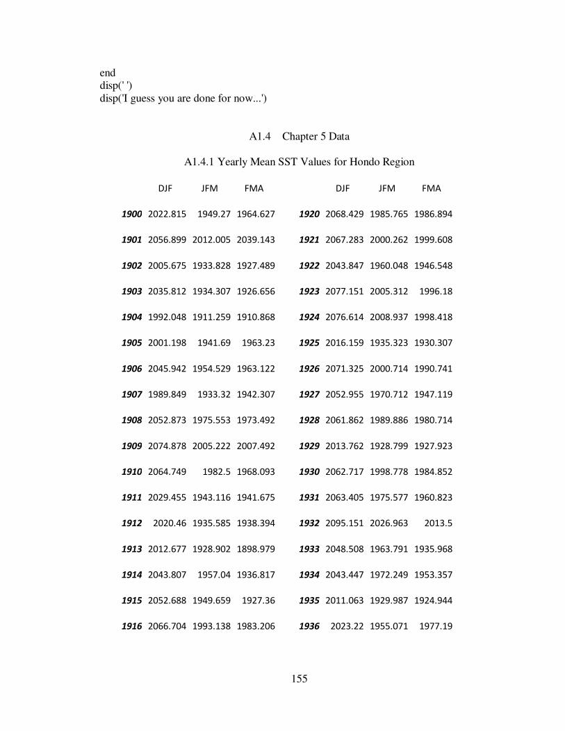
155
end disp(' ') disp('I guess you are done for now...')
A1.4 Chapter 5 Data
A1.4.1 Yearly Mean SST Values for Hondo Region
DJF JFM FMA DJF JFM FMA
1900 2022.815 1949.27 1964.627 1920 2068.429 1985.765 1986.894
1901 2056.899 2012.005 2039.143 1921 2067.283 2000.262 1999.608
1902 2005.675 1933.828 1927.489 1922 2043.847 1960.048 1946.548
1903 2035.812 1934.307 1926.656 1923 2077.151 2005.312 1996.18
1904 1992.048 1911.259 1910.868 1924 2076.614 2008.937 1998.418
1905 2001.198 1941.69 1963.23 1925 2016.159 1935.323 1930.307
1906 2045.942 1954.529 1963.122 1926 2071.325 2000.714 1990.741
1907 1989.849 1933.32 1942.307 1927 2052.955 1970.712 1947.119
1908 2052.873 1975.553 1973.492 1928 2061.862 1989.886 1980.714
1909 2074.878 2005.222 2007.492 1929 2013.762 1928.799 1927.923
1910 2064.749 1982.5 1968.093 1930 2062.717 1998.778 1984.852
1911 2029.455 1943.116 1941.675 1931 2063.405 1975.577 1960.823
1912 2020.46 1935.585 1938.394 1932 2095.151 2026.963 2013.5
1913 2012.677 1928.902 1898.979 1933 2048.508 1963.791 1935.968
1914 2043.807 1957.04 1936.817 1934 2043.447 1972.249 1953.357
1915 2052.688 1949.659 1927.36 1935 2011.063 1929.987 1924.944
1916 2066.704 1993.138 1983.206 1936 2023.22 1955.071 1977.19
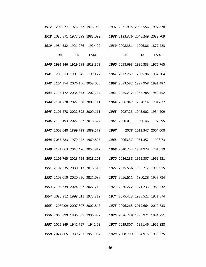
156
1917 2049.77 1976.937 1976.082 1937 2071.915 2002.556 1997.878
1918 2030.571 1977.698 1985.098 1938 2123.376 2046.249 2033.709
1919 1984.532 1921.976 1924.22 1939 2008.381 1906.86 1877.423
DJF JFM FMA DJF JFM FMA
1940 1991.146 1919.598 1918.323 1960 2058.693 1986.333 1976.765
1941 2058.13 1991.045 1990.27 1961 2072.267 2005.96 1987.304
1942 2164.354 2076.156 2058.005 1962 2083.582 1999.958 1991.487
1943 2115.172 2034.873 2023.27 1963 2055.212 1967.788 1949.452
1944 2101.278 2022.698 2009.111 1964 2086.942 2020.14 2017.77
1945 2101.278 2022.698 2009.111 1965 2027.23 1943.902 1934.209
1946 2115.193 2027.587 2016.627 1966 2060.011 1996.46 1978.95
1947 2002.648 1899.728 1889.579 1967 2078 2013.347 2004.008
1948 2056.783 1979.442 1969.825 1968 2063.37 1951.352 1928.73
1949 2121.063 2047.476 2057.817 1969 2040.754 1984.979 2013.19
1950 2101.765 2023.754 2028.101 1970 2026.238 1955.307 1969.921
1951 2102.235 2030.913 2016.519 1971 2075.556 1995.212 1996.915
1952 2102.019 2020.336 2021.098 1972 2056.611 1960.28 1937.794
1953 2106.339 2024.807 2027.212 1973 2026.222 1971.233 1989.532
1954 2085.312 1998.011 1977.312 1974 2075.423 1985.521 1971.574
1955 2080.09 2007.807 2002.847 1975 2096.265 2019.664 2010.733
1956 2063.899 1996.505 1996.897 1976 2076.728 1995.921 1994.751
1957 2022.849 1941.767 1942.28 1977 2029.807 1951.46 1955.828
1958 2024.865 1939.791 1951.934 1978 2008.799 1934.915 1939.325
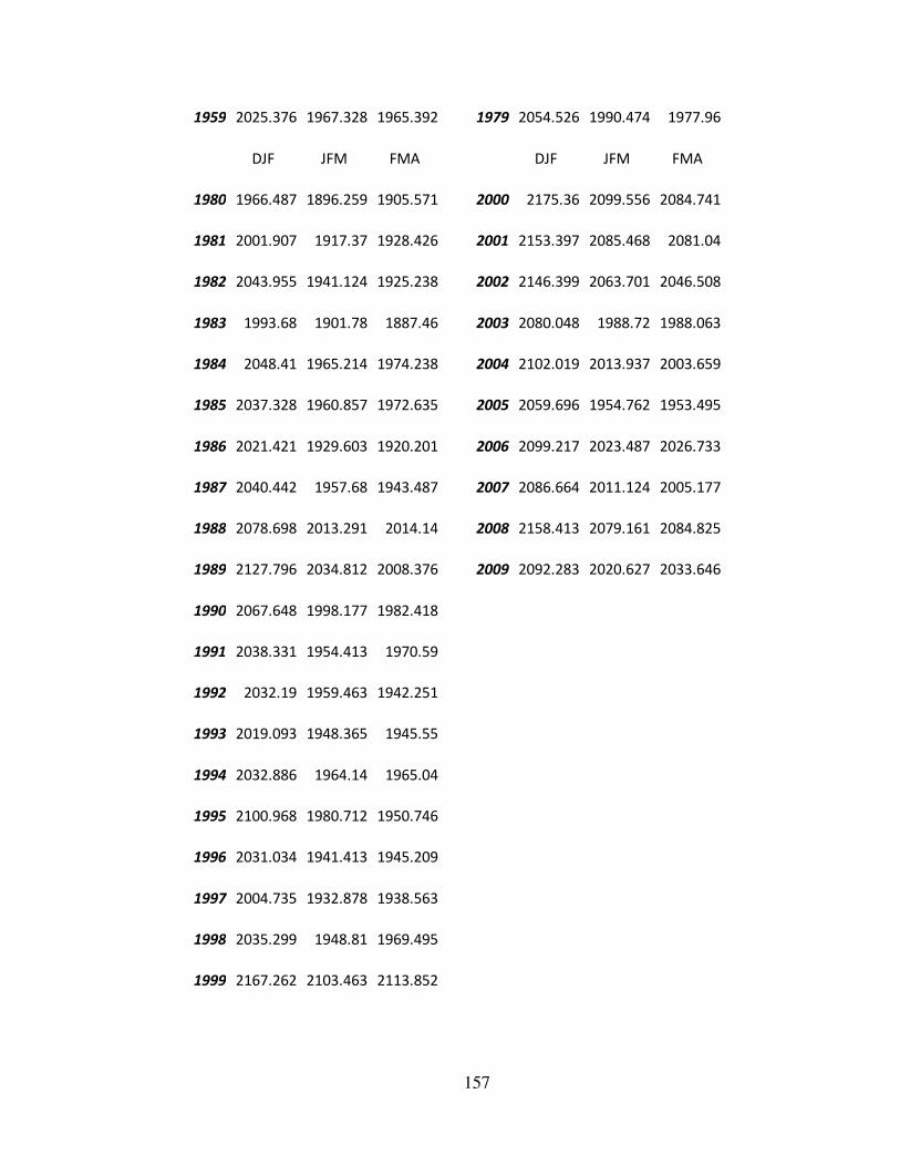
157
1959 2025.376 1967.328 1965.392 1979 2054.526 1990.474 1977.96
DJF JFM FMA DJF JFM FMA
1980 1966.487 1896.259 1905.571 2000 2175.36 2099.556 2084.741
1981 2001.907 1917.37 1928.426 2001 2153.397 2085.468 2081.04
1982 2043.955 1941.124 1925.238 2002 2146.399 2063.701 2046.508
1983 1993.68 1901.78 1887.46 2003 2080.048 1988.72 1988.063
1984 2048.41 1965.214 1974.238 2004 2102.019 2013.937 2003.659
1985 2037.328 1960.857 1972.635 2005 2059.696 1954.762 1953.495
1986 2021.421 1929.603 1920.201 2006 2099.217 2023.487 2026.733
1987 2040.442 1957.68 1943.487 2007 2086.664 2011.124 2005.177
1988 2078.698 2013.291 2014.14 2008 2158.413 2079.161 2084.825
1989 2127.796 2034.812 2008.376 2009 2092.283 2020.627 2033.646
1990 2067.648 1998.177 1982.418
1991 2038.331 1954.413 1970.59
1992 2032.19 1959.463 1942.251
1993 2019.093 1948.365 1945.55
1994 2032.886 1964.14 1965.04
1995 2100.968 1980.712 1950.746
1996 2031.034 1941.413 1945.209
1997 2004.735 1932.878 1938.563
1998 2035.299 1948.81 1969.495
1999 2167.262 2103.463 2113.852
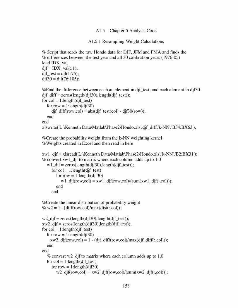
158
A1.5 Chapter 5 Analysis Code
A1.5.1 Resampling Weight Calculations
% Script that reads the raw Hondo data for DJF, JFM and FMA and finds the % differences between the test year and all 30 calibration years (1976-05) load IDX_val djf = IDX_val(:,1); djf_test = djf(1:75); djf30 = djf(76:105); %Find the difference between each an element in djf_test, and each element in djf30. djf_diff = zeros(length(djf30),length(djf_test)); for col = 1:length(djf_test) for row = 1:length(djf30) djf_diff(row,col) = abs(djf_test(col) - djf30(row)); end end xlswrite('L:\Kenneth Data\Matlab\Phase2\Hondo.xls',djf_diff,'k-NN','B34:BX63'); %Create the probability weight from the k-NN weighting kernel %Weights created in Excel and then read in here xw1_djf = xlsread('L:\Kenneth Data\Matlab\Phase2\Hondo.xls','k-NN','B2:BX31'); % convert xw1_djf to matrix where each column adds up to 1.0 w1_djf = zeros(length(djf30),length(djf_test)); for col = 1:length(djf_test) for row = 1:length(djf30) w1_djf(row,col) = xw1_djf(row,col)/(sum(xw1_djf(:,col))); end end %Create the linear distribution of probability weight % w2 = 1 - [diff(row,col)/max(dist(:,col))] w2_djf = zeros(length(djf30),length(djf_test)); xw2_djf = zeros(length(djf30),length(djf_test)); for col = 1:length(djf_test) for row = 1:length(djf30) xw2_djf(row,col) = 1 - (djf_diff(row,col)/max(djf_diff(:,col))); end end % convert w2_djf to matrix where each column adds up to 1.0 for col = 1:length(djf_test) for row = 1:length(djf30) w2_djf(row,col) = xw2_djf(row,col)/(sum(xw2_djf(:,col)));
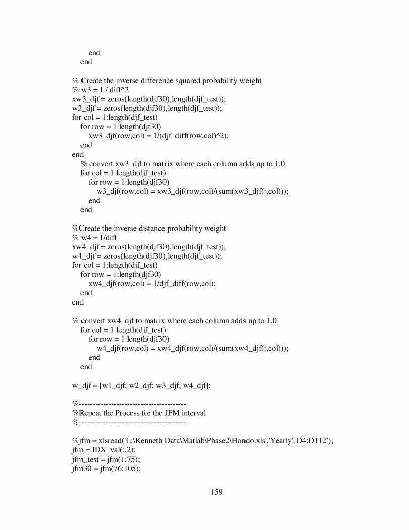
159
end end % Create the inverse difference squared probability weight % w3 = 1 / diff^2 xw3_djf = zeros(length(djf30),length(djf_test)); w3_djf = zeros(length(djf30),length(djf_test)); for col = 1:length(djf_test) for row = 1:length(djf30) xw3_djf(row,col) = 1/(djf_diff(row,col)^2); end end % convert xw3_djf to matrix where each column adds up to 1.0 for col = 1:length(djf_test) for row = 1:length(djf30) w3_djf(row,col) = xw3_djf(row,col)/(sum(xw3_djf(:,col))); end end %Create the inverse distance probability weight % w4 = 1/diff xw4_djf = zeros(length(djf30),length(djf_test)); w4_djf = zeros(length(djf30),length(djf_test)); for col = 1:length(djf_test) for row = 1:length(djf30) xw4_djf(row,col) = 1/djf_diff(row,col); end end % convert xw4_djf to matrix where each column adds up to 1.0 for col = 1:length(djf_test) for row = 1:length(djf30) w4_djf(row,col) = xw4_djf(row,col)/(sum(xw4_djf(:,col))); end end w_djf = [w1_djf; w2_djf; w3_djf; w4_djf]; %---------------------------------------- %Repeat the Process for the JFM interval %---------------------------------------- %jfm = xlsread('L:\Kenneth Data\Matlab\Phase2\Hondo.xls','Yearly','D4:D112'); jfm = IDX_val(:,2); jfm_test = jfm(1:75); jfm30 = jfm(76:105);

160
%Find the difference between each an element in jfm_test, and each element %in jfm30. jfm_diff = zeros(30,length(jfm_test)); for col = 1:length(jfm_test) for row = 1:length(jfm30) jfm_diff(row,col) = abs(jfm_test(col) - jfm30(row)); end end xlswrite('L:\Kenneth Data\Matlab\Phase2\Hondo.xls',jfm_diff,'k-NN','B34:BX63'); %Create the probability weight from the k-NN weighting kernel %Weights created in Excel and then read in here xw1_jfm = xlsread('L:\Kenneth Data\Matlab\Phase2\Hondo.xls','k-NN','B2:BX31'); % convert xw1_jfm to matrix where each column adds up to 1.0 w1_jfm = zeros(length(jfm30),length(jfm_test)); for col = 1:length(jfm_test) for row = 1:length(jfm30) w1_jfm(row,col) = xw1_jfm(row,col)/(sum(xw1_jfm(:,col))); end end %Create the linear distribution of probability weight % w2 = 1 - [diff(row,col)/max(dist(:,col))] w2_jfm = zeros(length(jfm30),length(jfm_test)); xw2_jfm = zeros(length(jfm30),length(jfm_test)); for col = 1:length(djf_test) for row = 1:length(jfm30) xw2_jfm(row,col) = 1 - (jfm_diff(row,col)/max(jfm_diff(:,col))); end end % convert w2_jfm to matrix where each column adds up to 1.0 for col = 1:length(jfm_test) for row = 1:length(jfm30) w2_jfm(row,col) = xw2_jfm(row,col)/(sum(xw2_jfm(:,col))); end end % Create the inverse difference squared probability weight % w3 = 1 / diff^2 xw3_jfm = zeros(length(jfm30),length(jfm_test)); w3_jfm = zeros(length(jfm30),length(jfm_test)); for col = 1:length(jfm_test)
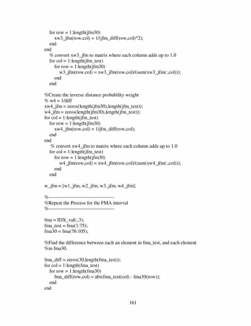
161
for row = 1:length(jfm30) xw3_jfm(row,col) = 1/(jfm_diff(row,col)^2); end end % convert xw3_jfm to matrix where each column adds up to 1.0 for col = 1:length(jfm_test) for row = 1:length(jfm30) w3_jfm(row,col) = xw3_jfm(row,col)/(sum(xw3_jfm(:,col))); end end %Create the inverse distance probability weight % w4 = 1/diff xw4_jfm = zeros(length(jfm30),length(jfm_test)); w4_jfm = zeros(length(jfm30),length(jfm_test)); for col = 1:length(jfm_test) for row = 1:length(jfm30) xw4_jfm(row,col) = 1/jfm_diff(row,col); end end % convert xw4_jfm to matrix where each column adds up to 1.0 for col = 1:length(jfm_test) for row = 1:length(jfm30) w4_jfm(row,col) = xw4_jfm(row,col)/(sum(xw4_jfm(:,col))); end end w_jfm = [w1_jfm; w2_jfm; w3_jfm; w4_jfm]; %---------------------------------------- %Repeat the Process for the FMA interval %---------------------------------------- fma = IDX_val(:,3); fma_test = fma(1:75); fma30 = fma(76:105); %Find the difference between each an element in fma_test, and each element %in fma30. fma_diff = zeros(30,length(fma_test)); for col = 1:length(fma_test) for row = 1:length(fma30) fma_diff(row,col) = abs(fma_test(col) - fma30(row)); end end

162
xlswrite('L:\Kenneth Data\Matlab\Phase2\Hondo.xls',fma_diff,'k-NN','B34:BX63'); %Create the probability weight from the k-NN weighting kernel %Weights created in Excel and then read in here xw1_fma = xlsread('L:\Kenneth Data\Matlab\Phase2\Hondo.xls','k-NN','B2:BX31'); % convert xw1_fma to matrix where each column adds up to 1.0 w1_fma = zeros(length(fma30),length(fma_test)); for col = 1:length(fma_test) for row = 1:length(fma30) w1_fma(row,col) = xw1_fma(row,col)/(sum(xw1_fma(:,col))); end end %Create the linear distribution of probability weight % w2 = 1 - [diff(row,col)/max(dist(:,col))] w2_fma = zeros(length(fma30),length(fma_test)); xw2_fma = zeros(length(fma30),length(fma_test)); for col = 1:length(fma_test) for row = 1:length(fma30) xw2_fma(row,col) = 1 - (fma_diff(row,col)/max(fma_diff(:,col))); end end % convert w2_fma to matrix where each column adds up to 1.0 for col = 1:length(fma_test) for row = 1:length(fma30) w2_fma(row,col) = xw2_fma(row,col)/(sum(xw2_fma(:,col))); end end % Create the inverse difference squared probability weight % w3 = 1 / diff^2 xw3_fma = zeros(length(fma30),length(fma_test)); w3_fma = zeros(length(fma30),length(fma_test)); for col = 1:length(fma_test) for row = 1:length(fma30) xw3_fma(row,col) = 1/(fma_diff(row,col)^2); end end % convert xw3_fma to matrix where each column adds up to 1.0 for col = 1:length(fma_test) for row = 1:length(fma30) w3_fma(row,col) = xw3_fma(row,col)/(sum(xw3_fma(:,col))); end end

163
%Create the inverse distance probability weight % w4 = 1/diff xw4_fma = zeros(length(fma30),length(fma_test)); w4_fma = zeros(length(fma30),length(fma_test)); for col = 1:length(fma_test) for row = 1:length(fma30) xw4_fma(row,col) = 1/fma_diff(row,col); end end % convert xw4_fma to matrix where each column adds up to 1.0 for col = 1:length(fma_test) for row = 1:length(fma30) w4_fma(row,col) = xw4_fma(row,col)/(sum(xw4_fma(:,col))); end end w_fma = [w1_fma; w2_fma; w3_fma; w4_fma]; %---------------------------------------- %Repeat the Process for the Water Year Average interval %---------------------------------------- yr = IDX_val(:,4); yr_test = yr(1:75); yr30 = yr(76:105); %Find the difference between each an element in yr_test, and each element %in yr30. yr_diff = zeros(length(yr30),length(yr_test)); for col = 1:length(yr_test) for row = 1:length(yr30) yr_diff(row,col) = abs(yr_test(col) - yr30(row)); end end xlswrite('L:\Kenneth Data\Matlab\Phase2\Hondo.xls',yr_diff,'k-NN','B34:BX63'); %Create the probability weight from the k-NN weighting kernel %Weights created in Excel and then read in here xw1_yr = xlsread('L:\Kenneth Data\Matlab\Phase2\Hondo.xls','k-NN','B2:BX31'); % convert w1_yr to matrix where each column adds up to 1.0 w1_yr = zeros(length(yr30),length(yr_test));
164
for col = 1:length(yr_test) for row = 1:length(yr30) w1_yr(row,col) = xw1_yr(row,col)/(sum(xw1_yr(:,col))); end end %Create the linear distribution of probability weight % w2 = 1 - [diff(row,col)/max(dist(:,col))] w2_yr = zeros(length(yr30),length(yr_test)); xw2_yr = zeros(length(yr30),length(yr_test)); for col = 1:length(yr_test) for row = 1:length(yr30) xw2_yr(row,col) = 1 - (yr_diff(row,col)/max(yr_diff(:,col))); end end % convert w2_yr to matrix where each column adds up to 1.0 for col = 1:length(yr_test) for row = 1:length(yr30) w2_yr(row,col) = xw2_yr(row,col)/(sum(xw2_yr(:,col))); end end % Create the inverse difference squared probability weight % w3 = 1 / diff^2 xw3_yr = zeros(length(yr30),length(yr_test)); w3_yr = zeros(length(yr30),length(yr_test)); for col = 1:length(yr_test) for row = 1:length(yr30) xw3_yr(row,col) = 1/(yr_diff(row,col)^2); end end % convert xw3_yr to matrix where each column adds up to 1.0 for col = 1:length(yr_test) for row = 1:length(yr30) w3_yr(row,col) = xw3_yr(row,col)/(sum(xw3_yr(:,col))); end end %Create the inverse distance probability weight % w4 = 1/diff xw4_yr = zeros(length(yr30),length(yr_test)); w4_yr = zeros(length(yr30),length(yr_test)); for col = 1:length(yr_test) for row = 1:length(yr30) xw4_yr(row,col) = 1/yr_diff(row,col); end
165
end % convert xw4_yr to matrix where each column adds up to 1.0 for col = 1:length(yr_test) for row = 1:length(yr30) w4_yr(row,col) = xw4_yr(row,col)/(sum(xw4_yr(:,col))); end end w_yr = [w1_yr; w2_yr; w3_yr; w4_yr]; aaa = [w_djf w_jfm w_fma w_yr]; [dim1 dim2] = size(aaa); w_0675 = reshape(aaa,dim1,dim2/4,4); save w_0675 w_0675
A1.5.2 Forecast Creation
%THIS CODE CALCUALTES FORECAST VALUES FOR 1906 - 1975 USING THE WEIGHTED %RESAMPLING (1,000 TIMES) AND THEN FINDS THE MEAN OF EACH RESAMPLE, THEN %THE MEAN OF ALL RESAMPLING TO OBTAIN THE FORECAST VALUE. % RUN TIME: 105 minutes %------------------------------------- %Read in the weights %------------------------------------- load w_0675 djf_wall = w_0675(:,:,1); jfm_wall = w_0675(:,:,2); fma_wall = w_0675(:,:,3); % From this dataset, the lagged relationships can be defined by using the % following columns from the *_wall matrices created above: %0-year lag: 6:75 (1906 - 1975) %1-year lag: 5:74 (1905 - 1974) %2-year lag: 4:73 (1904 - 1973) %Total forecasts created at each location = 70 %------------------------------------- % Read in the observed data %------------------------------------- %qoyr_all = xlsread('L:/Kenneth Data/Matlab/Phase2/Hondo.xls','qobs-y','B2:AD103'); load qoyr_all

166
%Create matrices of observed values. Use the following to know which %observed values to be used: %Resampling Data: Rows 71:100 for qoyr_all (1976 - 2005) %Observation Data: Rows 1:70 (qoaj_all and qoyr_all) 1906 - 1975 %Observed Data Matrix qo = qoyr_all(1:70,:); %Resampling Data Matrix qoy = qoyr_all(71:100,:); %Create matrix of forecasts using just the 30-yr average f30 = mean(qoy); %-------------------------------------- % Run Analysis on DJF | Lag = 0 Year %-------------------------------------- djf_0_w1 = djf_wall(1:30,6:75); djf_0_w2 = djf_wall(31:60,6:75); djf_0_w3 = djf_wall(61:90,6:75); djf_0_w4 = djf_wall(91:120,6:75); %Create matrix of forecast values djf_0_qfall1 = zeros(29,70,1000); djf_0_qfall2 = zeros(29,70,1000); djf_0_qfall3 = zeros(29,70,1000); djf_0_qfall4 = zeros(29,70,1000); for loc = 1:29 for yr = 1:70 for l = 1:1000 djf_0_qfall1(loc,yr,l) = mean(randsample(qoy(:,loc),length(djf_0_w1),true,djf_0_w1(:,yr))); djf_0_qfall2(loc,yr,l) = mean(randsample(qoy(:,loc),length(djf_0_w2),true,djf_0_w2(:,yr))); djf_0_qfall3(loc,yr,l) = mean(randsample(qoy(:,loc),length(djf_0_w3),true,djf_0_w3(:,yr))); djf_0_qfall4(loc,yr,l) = mean(randsample(qoy(:,loc),length(djf_0_w4),true,djf_0_w4(:,yr))); end end end djf_0_qf1 = transpose(mean(djf_0_qfall1,3)); djf_0_qf2 = transpose(mean(djf_0_qfall2,3));

167
djf_0_qf3 = transpose(mean(djf_0_qfall3,3)); djf_0_qf4 = transpose(mean(djf_0_qfall4,3)); %-------------------------------------- % Run Analysis on DJF | Lag = 1 Year %-------------------------------------- djf_1_w1 = djf_wall(1:30,5:74); djf_1_w2 = djf_wall(31:60,5:74); djf_1_w3 = djf_wall(61:90,5:74); djf_1_w4 = djf_wall(91:120,5:74); %Create matrix of forecast values djf_1_qfall1 = zeros(29,70,1000); djf_1_qfall2 = zeros(29,70,1000); djf_1_qfall3 = zeros(29,70,1000); djf_1_qfall4 = zeros(29,70,1000); for loc = 1:29 for yr = 1:70 for l = 1:1000 djf_1_qfall1(loc,yr,l) = mean(randsample(qoy(:,loc),length(djf_1_w1),true,djf_1_w1(:,yr))); djf_1_qfall2(loc,yr,l) = mean(randsample(qoy(:,loc),length(djf_1_w2),true,djf_1_w2(:,yr))); djf_1_qfall3(loc,yr,l) = mean(randsample(qoy(:,loc),length(djf_1_w3),true,djf_1_w3(:,yr))); djf_1_qfall4(loc,yr,l) = mean(randsample(qoy(:,loc),length(djf_1_w4),true,djf_1_w4(:,yr))); end end end djf_1_qf1 = transpose(mean(djf_1_qfall1,3)); djf_1_qf2 = transpose(mean(djf_1_qfall2,3)); djf_1_qf3 = transpose(mean(djf_1_qfall3,3)); djf_1_qf4 = transpose(mean(djf_1_qfall4,3)); %-------------------------------------- % Run Analysis on DJF | Lag = 2 Year %-------------------------------------- djf_2_w1 = djf_wall(1:30,4:73); djf_2_w2 = djf_wall(31:60,4:73); djf_2_w3 = djf_wall(61:90,4:73); djf_2_w4 = djf_wall(91:120,4:73);
168
%Create matrix of forecast values djf_2_qfall1 = zeros(29,70,1000); djf_2_qfall2 = zeros(29,70,1000); djf_2_qfall3 = zeros(29,70,1000); djf_2_qfall4 = zeros(29,70,1000); for loc = 1:29 for yr = 1:70 for l = 1:1000 djf_2_qfall1(loc,yr,l) = mean(randsample(qoy(:,loc),length(djf_2_w1),true,djf_2_w1(:,yr))); djf_2_qfall2(loc,yr,l) = mean(randsample(qoy(:,loc),length(djf_2_w2),true,djf_2_w2(:,yr))); djf_2_qfall3(loc,yr,l) = mean(randsample(qoy(:,loc),length(djf_2_w3),true,djf_2_w3(:,yr))); djf_2_qfall4(loc,yr,l) = mean(randsample(qoy(:,loc),length(djf_2_w4),true,djf_2_w4(:,yr))); end end end djf_2_qf1 = transpose(mean(djf_2_qfall1,3)); djf_2_qf2 = transpose(mean(djf_2_qfall2,3)); djf_2_qf3 = transpose(mean(djf_2_qfall3,3)); djf_2_qf4 = transpose(mean(djf_2_qfall4,3)); %-------------------------------------- % Run Analysis on JFM | Lag = 0 Year %-------------------------------------- jfm_0_w1 = jfm_wall(1:30,6:75); jfm_0_w2 = jfm_wall(31:60,6:75); jfm_0_w3 = jfm_wall(61:90,6:75); jfm_0_w4 = jfm_wall(91:120,6:75); %Create matrix of forecast values jfm_0_qfall1 = zeros(29,70,1000); jfm_0_qfall2 = zeros(29,70,1000); jfm_0_qfall3 = zeros(29,70,1000); jfm_0_qfall4 = zeros(29,70,1000); for loc = 1:29 for yr = 1:70 for l = 1:1000 jfm_0_qfall1(loc,yr,l) = mean(randsample(qoy(:,loc),length(jfm_0_w1),true,jfm_0_w1(:,yr)));

169
jfm_0_qfall2(loc,yr,l) = mean(randsample(qoy(:,loc),length(jfm_0_w2),true,jfm_0_w2(:,yr))); jfm_0_qfall3(loc,yr,l) = mean(randsample(qoy(:,loc),length(jfm_0_w3),true,jfm_0_w3(:,yr))); jfm_0_qfall4(loc,yr,l) = mean(randsample(qoy(:,loc),length(jfm_0_w4),true,jfm_0_w4(:,yr))); end end end jfm_0_qf1 = transpose(mean(jfm_0_qfall1,3)); jfm_0_qf2 = transpose(mean(jfm_0_qfall2,3)); jfm_0_qf3 = transpose(mean(jfm_0_qfall3,3)); jfm_0_qf4 = transpose(mean(jfm_0_qfall4,3)); %-------------------------------------- % Run Analysis on JFM | Lag = 1 Year %-------------------------------------- jfm_1_w1 = jfm_wall(1:30,5:74); jfm_1_w2 = jfm_wall(31:60,5:74); jfm_1_w3 = jfm_wall(61:90,5:74); jfm_1_w4 = jfm_wall(91:120,5:74); %Create matrix of forecast values jfm_1_qfall1 = zeros(29,70,1000); jfm_1_qfall2 = zeros(29,70,1000); jfm_1_qfall3 = zeros(29,70,1000); jfm_1_qfall4 = zeros(29,70,1000); for loc = 1:29 for yr = 1:70 for l = 1:1000 jfm_1_qfall1(loc,yr,l) = mean(randsample(qoy(:,loc),length(jfm_1_w1),true,jfm_1_w1(:,yr))); jfm_1_qfall2(loc,yr,l) = mean(randsample(qoy(:,loc),length(jfm_1_w2),true,jfm_1_w2(:,yr))); jfm_1_qfall3(loc,yr,l) = mean(randsample(qoy(:,loc),length(jfm_1_w3),true,jfm_1_w3(:,yr))); jfm_1_qfall4(loc,yr,l) = mean(randsample(qoy(:,loc),length(jfm_1_w4),true,jfm_1_w4(:,yr))); end end end jfm_1_qf1 = transpose(mean(jfm_1_qfall1,3)); jfm_1_qf2 = transpose(mean(jfm_1_qfall2,3));

170
jfm_1_qf3 = transpose(mean(jfm_1_qfall3,3)); jfm_1_qf4 = transpose(mean(jfm_1_qfall4,3)); %-------------------------------------- % Run Analysis on JFM | Lag = 2 Year %-------------------------------------- jfm_2_w1 = jfm_wall(1:30,4:73); jfm_2_w2 = jfm_wall(31:60,4:73); jfm_2_w3 = jfm_wall(61:90,4:73); jfm_2_w4 = jfm_wall(91:120,4:73); %Create matrix of forecast values jfm_2_qfall1 = zeros(29,70,1000); jfm_2_qfall2 = zeros(29,70,1000); jfm_2_qfall3 = zeros(29,70,1000); jfm_2_qfall4 = zeros(29,70,1000); for loc = 1:29 for yr = 1:70 for l = 1:1000 jfm_2_qfall1(loc,yr,l) = mean(randsample(qoy(:,loc),length(jfm_2_w1),true,jfm_2_w1(:,yr))); jfm_2_qfall2(loc,yr,l) = mean(randsample(qoy(:,loc),length(jfm_2_w2),true,jfm_2_w2(:,yr))); jfm_2_qfall3(loc,yr,l) = mean(randsample(qoy(:,loc),length(jfm_2_w3),true,jfm_2_w3(:,yr))); jfm_2_qfall4(loc,yr,l) = mean(randsample(qoy(:,loc),length(jfm_2_w4),true,jfm_2_w4(:,yr))); end end end jfm_2_qf1 = transpose(mean(jfm_2_qfall1,3)); jfm_2_qf2 = transpose(mean(jfm_2_qfall2,3)); jfm_2_qf3 = transpose(mean(jfm_2_qfall3,3)); jfm_2_qf4 = transpose(mean(jfm_2_qfall4,3)); %-------------------------------------- % Run Analysis on FMA | Lag = 0 Year %-------------------------------------- fma_0_w1 = fma_wall(1:30,6:75); fma_0_w2 = fma_wall(31:60,6:75); fma_0_w3 = fma_wall(61:90,6:75); fma_0_w4 = fma_wall(91:120,6:75);
171
%Create matrix of forecast values fma_0_qfall1 = zeros(29,70,1000); fma_0_qfall2 = zeros(29,70,1000); fma_0_qfall3 = zeros(29,70,1000); fma_0_qfall4 = zeros(29,70,1000); for loc = 1:29 for yr = 1:70 for l = 1:1000 fma_0_qfall1(loc,yr,l) = mean(randsample(qoy(:,loc),length(fma_0_w1),true,fma_0_w1(:,yr))); fma_0_qfall2(loc,yr,l) = mean(randsample(qoy(:,loc),length(fma_0_w2),true,fma_0_w2(:,yr))); fma_0_qfall3(loc,yr,l) = mean(randsample(qoy(:,loc),length(fma_0_w3),true,fma_0_w3(:,yr))); fma_0_qfall4(loc,yr,l) = mean(randsample(qoy(:,loc),length(fma_0_w4),true,fma_0_w4(:,yr))); end end end fma_0_qf1 = transpose(mean(fma_0_qfall1,3)); fma_0_qf2 = transpose(mean(fma_0_qfall2,3)); fma_0_qf3 = transpose(mean(fma_0_qfall3,3)); fma_0_qf4 = transpose(mean(fma_0_qfall4,3)); %-------------------------------------- % Forecasts FMA | Lag = 1 Year %-------------------------------------- fma_1_w1 = fma_wall(1:30,5:74); fma_1_w2 = fma_wall(31:60,5:74); fma_1_w3 = fma_wall(61:90,5:74); fma_1_w4 = fma_wall(91:120,5:74); %Create matrix of forecast values fma_1_qfall1 = zeros(29,70,1000); fma_1_qfall2 = zeros(29,70,1000); fma_1_qfall3 = zeros(29,70,1000); fma_1_qfall4 = zeros(29,70,1000); for loc = 1:29 for yr = 1:70 for l = 1:1000 fma_1_qfall1(loc,yr,l) = mean(randsample(qoy(:,loc),length(fma_1_w1),true,fma_1_w1(:,yr)));
172
fma_1_qfall2(loc,yr,l) = mean(randsample(qoy(:,loc),length(fma_1_w2),true,fma_1_w2(:,yr))); fma_1_qfall3(loc,yr,l) = mean(randsample(qoy(:,loc),length(fma_1_w3),true,fma_1_w3(:,yr))); fma_1_qfall4(loc,yr,l) = mean(randsample(qoy(:,loc),length(fma_1_w4),true,fma_1_w4(:,yr))); end end end fma_1_qf1 = transpose(mean(fma_1_qfall1,3)); fma_1_qf2 = transpose(mean(fma_1_qfall2,3)); fma_1_qf3 = transpose(mean(fma_1_qfall3,3)); fma_1_qf4 = transpose(mean(fma_1_qfall4,3)); %-------------------------------------- % Forecasts FMA | Lag = 2 Year %-------------------------------------- fma_2_w1 = fma_wall(1:30,4:73); fma_2_w2 = fma_wall(31:60,4:73); fma_2_w3 = fma_wall(61:90,4:73); fma_2_w4 = fma_wall(91:120,4:73); %Create matrix of forecast values fma_2_qfall1 = zeros(29,70,1000); fma_2_qfall2 = zeros(29,70,1000); fma_2_qfall3 = zeros(29,70,1000); fma_2_qfall4 = zeros(29,70,1000); for loc = 1:29 for yr = 1:70 for l = 1:1000 fma_2_qfall1(loc,yr,l) = mean(randsample(qoy(:,loc),length(fma_2_w1),true,fma_2_w1(:,yr))); fma_2_qfall2(loc,yr,l) = mean(randsample(qoy(:,loc),length(fma_2_w2),true,fma_2_w2(:,yr))); fma_2_qfall3(loc,yr,l) = mean(randsample(qoy(:,loc),length(fma_2_w3),true,fma_2_w3(:,yr))); fma_2_qfall4(loc,yr,l) = mean(randsample(qoy(:,loc),length(fma_2_w4),true,fma_2_w4(:,yr))); end end end fma_2_qf1 = transpose(mean(fma_2_qfall1,3)); fma_2_qf2 = transpose(mean(fma_2_qfall2,3));

173
fma_2_qf3 = transpose(mean(fma_2_qfall3,3)); fma_2_qf4 = transpose(mean(fma_2_qfall4,3)); %------------------------------------------ % Collect forecast values and write to Excel %------------------------------------------ f_djf_all = [djf_0_qf1 djf_0_qf2 djf_0_qf3 djf_0_qf4 ... djf_1_qf1 djf_1_qf2 djf_1_qf3 djf_1_qf4 ... djf_2_qf1 djf_2_qf2 djf_2_qf3 djf_2_qf4]; f_jfm_all = [jfm_0_qf1 jfm_0_qf2 jfm_0_qf3 jfm_0_qf4 ... jfm_1_qf1 jfm_1_qf2 jfm_1_qf3 jfm_1_qf4 ... jfm_2_qf1 jfm_2_qf2 jfm_2_qf3 jfm_2_qf4]; f_fma_all = [fma_0_qf1 fma_0_qf2 fma_0_qf3 fma_0_qf4 ... fma_1_qf1 fma_1_qf2 fma_1_qf3 fma_1_qf4 ... fma_2_qf1 fma_2_qf2 fma_2_qf3 fma_2_qf4]; %xlswrite('L:/Kenneth Data/Matlab/Phase2/Hondo_f.xls',f_djf_all', 'f_djf','C2'); %xlswrite('L:/Kenneth Data/Matlab/Phase2/Hondo_f.xls',f_jfm_all', 'f_jfm','C2'); %xlswrite('L:/Kenneth Data/Matlab/Phase2/Hondo_f.xls',f_fma_all', 'f_fma','C2'); %aaa = [f_djf_all f_jfm_all f_fma_all]; %[dim1 dim2] = size(aaa); %f_0675 = reshape(aaa,dim1,dim2/3,3); %save f_0675 f_0675
A1.5.3 LEPS Calculation
%Read in the observed data load qoyr_all %Create matrices of observed values. Use the following to know which %observed values to be used: %Resampling Data: Rows 71:100 for both qoaj_all and qoyr_all (1976 - 2005) %Observation Data: Rows 1:70 (qoaj_all and qoyr_all) 1906 - 1975 %Observed Data Matrix qoyr = qoyr_all(1:70,:); %Resampling Data Matrix qoy = qoyr_all(71:100,:); %Read in Forecast values created with the forecasts.m command load f_0675 djf_fall = f_0675(:,:,1); jfm_fall = f_0675(:,:,2);
174
fma_fall = f_0675(:,:,3); %--------------------------------------------- % Calculate for Lag = 0 Year %--------------------------------------------- %Create zero matrices yoy = zeros(70,29); djf_0_yf1 = zeros(70,29); djf_0_yf2 = zeros(70,29); djf_0_yf3 = zeros(70,29); djf_0_yf4 = zeros(70,29); djf_0_leps1 = zeros(70,29); djf_0_leps2 = zeros(70,29); djf_0_leps3 = zeros(70,29); djf_0_leps4 = zeros(70,29); djf_0_lepsmax1 = zeros(70,29); djf_0_lepsmax2 = zeros(70,29); djf_0_lepsmax3 = zeros(70,29); djf_0_lepsmax4 = zeros(70,29); lepsmin = zeros(70,29); djf_0_sk1 = zeros(29,1); djf_0_sk2 = zeros(29,1); djf_0_sk3 = zeros(29,1); djf_0_sk4 = zeros(29,1); %Divide out the forecast values into each alternative for this lag time djf_0_qf1 = djf_fall(:,1:29); djf_0_qf2 = djf_fall(:,30:58); djf_0_qf3 = djf_fall(:,59:87); djf_0_qf4 = djf_fall(:,88:116); %Find the Probabilities to define the y-axis of the eCDF. Create seperate %eCDF function for the Apr-Jul observations and the Yearly observations. P = transpose((1:size(qoyr,1))/(size(qoyr,1)+1)); %Find the probabilities of the observed (yo) and forecasted (yf) values %on the PDF by interpolating along the qopdf data. for loc = 1:29 for yr = 1:70 yoy(yr,loc) = interp1(sort(qoyr(:,loc)),P,qoyr(yr,loc),'linear','extrap' ); djf_0_yf1(yr,loc) = interp1(sort(qoyr(:,loc)),P,djf_0_qf1(yr,loc),'linear','extrap' ); djf_0_yf2(yr,loc) = interp1(sort(qoyr(:,loc)),P,djf_0_qf2(yr,loc),'linear','extrap' ); djf_0_yf3(yr,loc) = interp1(sort(qoyr(:,loc)),P,djf_0_qf3(yr,loc),'linear','extrap' ); djf_0_yf4(yr,loc) = interp1(sort(qoyr(:,loc)),P,djf_0_qf4(yr,loc),'linear','extrap' );

175
end end % Calculate the min LEPS Scores possible from the April-July and Yearly % volumes for loc = 1:29 for yr = 1:70 if yoy(yr,loc)>=0.5 lepsmin(yr,loc) = (3*(1-abs(0 - yoy(yr,loc)) + yoy(yr,loc)^2 - yoy(yr,loc)) - 1); else lepsmin(yr,loc) = (3*(1-abs(1 - yoy(yr,loc)) + yoy(yr,loc)^2 - yoy(yr,loc)) - 1); end end end %Calculate the max possible LEPS scores for loc = 1:29 for yr = 1:70 djf_0_lepsmax1(yr,loc) = (3*(1-abs(djf_0_yf1(yr,loc) - djf_0_yf1(yr,loc))... + djf_0_yf1(yr,loc)^2 - djf_0_yf1(yr,loc) + djf_0_yf1(yr,loc)^2 - djf_0_yf1(yr,loc)) - 1); djf_0_lepsmax2(yr,loc) = (3*(1-abs(djf_0_yf2(yr,loc) - djf_0_yf2(yr,loc))... + djf_0_yf2(yr,loc)^2 - djf_0_yf2(yr,loc) + djf_0_yf2(yr,loc)^2 - djf_0_yf2(yr,loc)) - 1); djf_0_lepsmax3(yr,loc) = (3*(1-abs(djf_0_yf3(yr,loc) - djf_0_yf3(yr,loc))... + djf_0_yf3(yr,loc)^2 - djf_0_yf3(yr,loc) + djf_0_yf3(yr,loc)^2 - djf_0_yf3(yr,loc)) - 1); djf_0_lepsmax4(yr,loc) = (3*(1-abs(djf_0_yf4(yr,loc) - djf_0_yf4(yr,loc))... + djf_0_yf4(yr,loc)^2 - djf_0_yf4(yr,loc) + djf_0_yf4(yr,loc)^2 - djf_0_yf4(yr,loc)) - 1); end end %Calculate the LEPS scores from the yfx and the yo matrices for loc = 1:29 for yr = 1:70 djf_0_leps1(yr,loc) = (3*(1-abs(djf_0_yf1(yr,loc) - yoy(yr,loc))... + djf_0_yf1(yr,loc)^2 - djf_0_yf1(yr,loc) + yoy(yr,loc)^2 - yoy(yr,loc)) - 1); djf_0_leps2(yr,loc) = (3*(1-abs(djf_0_yf2(yr,loc) - yoy(yr,loc))... + djf_0_yf2(yr,loc)^2 - djf_0_yf2(yr,loc) + yoy(yr,loc)^2 - yoy(yr,loc)) - 1); djf_0_leps3(yr,loc) = (3*(1-abs(djf_0_yf3(yr,loc) - yoy(yr,loc))... + djf_0_yf3(yr,loc)^2 - djf_0_yf3(yr,loc) + yoy(yr,loc)^2 - yoy(yr,loc)) - 1); djf_0_leps4(yr,loc) = (3*(1-abs(djf_0_yf4(yr,loc) - yoy(yr,loc))... + djf_0_yf4(yr,loc)^2 - djf_0_yf4(yr,loc) + yoy(yr,loc)^2 - yoy(yr,loc)) - 1); end end

176
%Calculate the Average Skill score at each location for loc = 1:29 if sum(djf_0_leps1(:,loc))>=0 djf_0_sk1(loc) = sum(djf_0_leps1(:,loc))/sum(djf_0_lepsmax1(:,loc)); else djf_0_sk1(loc) = sum(djf_0_leps1(:,loc))/sum(lepsmin(:,loc)); end if sum(djf_0_leps2(:,loc))>=0 djf_0_sk2(loc) = sum(djf_0_leps2(:,loc))/sum(djf_0_lepsmax2(:,loc)); else djf_0_sk2(loc) = sum(djf_0_leps2(:,loc))/sum(lepsmin(:,loc)); end if sum(djf_0_leps3(:,loc))>=0 djf_0_sk3(loc) = sum(djf_0_leps3(:,loc))/sum(djf_0_lepsmax3(:,loc)); else djf_0_sk3(loc) = sum(djf_0_leps3(:,loc))/sum(lepsmin(:,loc)); end if sum(djf_0_leps4(:,loc))>=0 djf_0_sk4(loc) = sum(djf_0_leps4(:,loc))/sum(djf_0_lepsmax4(:,loc)); else djf_0_sk4(loc) = sum(djf_0_leps4(:,loc))/sum(lepsmin(:,loc)); end end djf_0_sk = 100*[djf_0_sk1 djf_0_sk2 djf_0_sk3 djf_0_sk4]; %--------------------------------------------- % Recalculate for Lag = 1Year %--------------------------------------------- %Divide weight data into each weight for the lag 1 alternative djf_1_yf1 = zeros(70,29); djf_1_yf2 = zeros(70,29); djf_1_yf3 = zeros(70,29); djf_1_yf4 = zeros(70,29); djf_1_leps1 = zeros(70,29); djf_1_leps2 = zeros(70,29); djf_1_leps3 = zeros(70,29); djf_1_leps4 = zeros(70,29); djf_1_lepsmax1 = zeros(70,29); djf_1_lepsmax2 = zeros(70,29); djf_1_lepsmax3 = zeros(70,29); djf_1_lepsmax4 = zeros(70,29); djf_1_sk1 = zeros(29,1); djf_1_sk2 = zeros(29,1);
177
djf_1_sk3 = zeros(29,1); djf_1_sk4 = zeros(29,1); %Divide out the forecast values into each alternative for this lag time djf_1_qf1 = djf_fall(:,117:145); djf_1_qf2 = djf_fall(:,146:174); djf_1_qf3 = djf_fall(:,175:203); djf_1_qf4 = djf_fall(:,204:232); %Find the Probabilities to define the y-axis of the eCDF. Create seperate %eCDF function for the Apr-Jul observations and the Yearly observations. P = transpose((1:size(qoyr,1))/(size(qoyr,1)+1)); %Find the probabilities of the observed (yo) and forecasted (yf) values %on the PDF by interpolating along the qopdf data. for loc = 1:29 for yr = 1:70 yoy(yr,loc) = interp1(sort(qoyr(:,loc)),P,qoyr(yr,loc),'linear','extrap' ); djf_1_yf1(yr,loc) = interp1(sort(qoyr(:,loc)),P,djf_1_qf1(yr,loc),'linear','extrap' ); djf_1_yf2(yr,loc) = interp1(sort(qoyr(:,loc)),P,djf_1_qf2(yr,loc),'linear','extrap' ); djf_1_yf3(yr,loc) = interp1(sort(qoyr(:,loc)),P,djf_1_qf3(yr,loc),'linear','extrap' ); djf_1_yf4(yr,loc) = interp1(sort(qoyr(:,loc)),P,djf_1_qf4(yr,loc),'linear','extrap' ); end end %Calculate the max possible LEPS scores for loc = 1:29 for yr = 1:70 djf_1_lepsmax1(yr,loc) = (3*(1-abs(djf_1_yf1(yr,loc) - djf_1_yf1(yr,loc))... + djf_1_yf1(yr,loc)^2 - djf_1_yf1(yr,loc) + djf_1_yf1(yr,loc)^2 - djf_1_yf1(yr,loc)) - 1); djf_1_lepsmax2(yr,loc) = (3*(1-abs(djf_1_yf2(yr,loc) - djf_1_yf2(yr,loc))... + djf_1_yf2(yr,loc)^2 - djf_1_yf2(yr,loc) + djf_1_yf2(yr,loc)^2 - djf_1_yf2(yr,loc)) - 1); djf_1_lepsmax3(yr,loc) = (3*(1-abs(djf_1_yf3(yr,loc) - djf_1_yf3(yr,loc))... + djf_1_yf3(yr,loc)^2 - djf_1_yf3(yr,loc) + djf_1_yf3(yr,loc)^2 - djf_1_yf3(yr,loc)) - 1); djf_1_lepsmax4(yr,loc) = (3*(1-abs(djf_1_yf4(yr,loc) - djf_1_yf4(yr,loc))... + djf_1_yf4(yr,loc)^2 - djf_1_yf4(yr,loc) + djf_1_yf4(yr,loc)^2 - djf_1_yf4(yr,loc)) - 1); end end %Calculate the LEPS scores from the yfx and the yo matrices for loc = 1:29

178
for yr = 1:70 djf_1_leps1(yr,loc) = (3*(1-abs(djf_1_yf1(yr,loc) - yoy(yr,loc))... + djf_1_yf1(yr,loc)^2 - djf_1_yf1(yr,loc) + yoy(yr,loc)^2 - yoy(yr,loc)) - 1); djf_1_leps2(yr,loc) = (3*(1-abs(djf_1_yf2(yr,loc) - yoy(yr,loc))... + djf_1_yf2(yr,loc)^2 - djf_1_yf2(yr,loc) + yoy(yr,loc)^2 - yoy(yr,loc)) - 1); djf_1_leps3(yr,loc) = (3*(1-abs(djf_1_yf3(yr,loc) - yoy(yr,loc))... + djf_1_yf3(yr,loc)^2 - djf_1_yf3(yr,loc) + yoy(yr,loc)^2 - yoy(yr,loc)) - 1); djf_1_leps4(yr,loc) = (3*(1-abs(djf_1_yf4(yr,loc) - yoy(yr,loc))... + djf_1_yf4(yr,loc)^2 - djf_1_yf4(yr,loc) + yoy(yr,loc)^2 - yoy(yr,loc)) - 1); end end %Calculate the Average Skill score at each location for loc = 1:29 if sum(djf_1_leps1(:,loc))>=0 djf_1_sk1(loc) = sum(djf_1_leps1(:,loc))/sum(djf_1_lepsmax1(:,loc)); else djf_1_sk1(loc) = sum(djf_1_leps1(:,loc))/sum(lepsmin(:,loc)); end if sum(djf_1_leps2(:,loc))>=0 djf_1_sk2(loc) = sum(djf_1_leps2(:,loc))/sum(djf_1_lepsmax2(:,loc)); else djf_1_sk2(loc) = sum(djf_1_leps2(:,loc))/sum(lepsmin(:,loc)); end if sum(djf_1_leps3(:,loc))>=0 djf_1_sk3(loc) = sum(djf_1_leps3(:,loc))/sum(djf_1_lepsmax3(:,loc)); else djf_1_sk3(loc) = sum(djf_1_leps3(:,loc))/sum(lepsmin(:,loc)); end if sum(djf_1_leps4(:,loc))>=0 djf_1_sk4(loc) = sum(djf_1_leps4(:,loc))/sum(djf_1_lepsmax4(:,loc)); else djf_1_sk4(loc) = sum(djf_1_leps4(:,loc))/sum(lepsmin(:,loc)); end end djf_1_sk = 100*[djf_1_sk1 djf_1_sk2 djf_1_sk3 djf_1_sk4]; %--------------------------------------------- % Recalculate for Lag = 2 Years %--------------------------------------------- djf_2_yf1 = zeros(70,29); djf_2_yf2 = zeros(70,29); djf_2_yf3 = zeros(70,29); djf_2_yf4 = zeros(70,29);

179
djf_2_leps1 = zeros(70,29); djf_2_leps2 = zeros(70,29); djf_2_leps3 = zeros(70,29); djf_2_leps4 = zeros(70,29); djf_2_lepsmax1 = zeros(70,29); djf_2_lepsmax2 = zeros(70,29); djf_2_lepsmax3 = zeros(70,29); djf_2_lepsmax4 = zeros(70,29); djf_2_sk1 = zeros(29,1); djf_2_sk2 = zeros(29,1); djf_2_sk3 = zeros(29,1); djf_2_sk4 = zeros(29,1); %Divide out the forecast values into each alternative for this lag time djf_2_qf1 = djf_fall(:,233:261); djf_2_qf2 = djf_fall(:,262:290); djf_2_qf3 = djf_fall(:,291:319); djf_2_qf4 = djf_fall(:,320:348); %Find the Probabilities to define the y-axis of the eCDF. Create seperate %eCDF function for the Apr-Jul observations and the Yearly observations. P = transpose((1:size(qoyr,1))/(size(qoyr,1)+1)); %Find the probabilities of the observed (yo) and forecasted (yf) values %on the PDF by interpolating along the qopdf data. for loc = 1:29 for yr = 1:70 yoy(yr,loc) = interp1(sort(qoyr(:,loc)),P,qoyr(yr,loc),'linear','extrap' ); djf_2_yf1(yr,loc) = interp1(sort(qoyr(:,loc)),P,djf_2_qf1(yr,loc),'linear','extrap' ); djf_2_yf2(yr,loc) = interp1(sort(qoyr(:,loc)),P,djf_2_qf2(yr,loc),'linear','extrap' ); djf_2_yf3(yr,loc) = interp1(sort(qoyr(:,loc)),P,djf_2_qf3(yr,loc),'linear','extrap' ); djf_2_yf4(yr,loc) = interp1(sort(qoyr(:,loc)),P,djf_2_qf4(yr,loc),'linear','extrap' ); end end %Calculate the max possible LEPS scores for loc = 1:29 for yr = 1:70 djf_2_lepsmax1(yr,loc) = (3*(1-abs(djf_2_yf1(yr,loc) - djf_2_yf1(yr,loc))... + djf_2_yf1(yr,loc)^2 - djf_2_yf1(yr,loc) + djf_2_yf1(yr,loc)^2 - djf_2_yf1(yr,loc)) - 1); djf_2_lepsmax2(yr,loc) = (3*(1-abs(djf_2_yf2(yr,loc) - djf_2_yf2(yr,loc))... + djf_2_yf2(yr,loc)^2 - djf_2_yf2(yr,loc) + djf_2_yf2(yr,loc)^2 - djf_2_yf2(yr,loc)) - 1); djf_2_lepsmax3(yr,loc) = (3*(1-abs(djf_2_yf3(yr,loc) - djf_2_yf3(yr,loc))...
180
+ djf_2_yf3(yr,loc)^2 - djf_2_yf3(yr,loc) + djf_2_yf3(yr,loc)^2 - djf_2_yf3(yr,loc)) - 1); djf_2_lepsmax4(yr,loc) = (3*(1-abs(djf_2_yf4(yr,loc) - djf_2_yf4(yr,loc))... + djf_2_yf4(yr,loc)^2 - djf_2_yf4(yr,loc) + djf_2_yf4(yr,loc)^2 - djf_2_yf4(yr,loc)) - 1); end end %Calculate the LEPS scores from the yfx and the yo matrices for loc = 1:29 for yr = 1:70 djf_2_leps1(yr,loc) = (3*(1-abs(djf_2_yf1(yr,loc) - yoy(yr,loc))... + djf_2_yf1(yr,loc)^2 - djf_2_yf1(yr,loc) + yoy(yr,loc)^2 - yoy(yr,loc)) - 1); djf_2_leps2(yr,loc) = (3*(1-abs(djf_2_yf2(yr,loc) - yoy(yr,loc))... + djf_2_yf2(yr,loc)^2 - djf_2_yf2(yr,loc) + yoy(yr,loc)^2 - yoy(yr,loc)) - 1); djf_2_leps3(yr,loc) = (3*(1-abs(djf_2_yf3(yr,loc) - yoy(yr,loc))... + djf_2_yf3(yr,loc)^2 - djf_2_yf3(yr,loc) + yoy(yr,loc)^2 - yoy(yr,loc)) - 1); djf_2_leps4(yr,loc) = (3*(1-abs(djf_2_yf4(yr,loc) - yoy(yr,loc))... + djf_2_yf4(yr,loc)^2 - djf_2_yf4(yr,loc) + yoy(yr,loc)^2 - yoy(yr,loc)) - 1); end end %Calculate the Average Skill score at each location for loc = 1:29 if sum(djf_2_leps1(:,loc))>=0 djf_2_sk1(loc) = sum(djf_2_leps1(:,loc))/sum(djf_2_lepsmax1(:,loc)); else djf_2_sk1(loc) = sum(djf_2_leps1(:,loc))/sum(lepsmin(:,loc)); end if sum(djf_2_leps2(:,loc))>=0 djf_2_sk2(loc) = sum(djf_2_leps2(:,loc))/sum(djf_2_lepsmax2(:,loc)); else djf_2_sk2(loc) = sum(djf_2_leps2(:,loc))/sum(lepsmin(:,loc)); end if sum(djf_2_leps3(:,loc))>=0 djf_2_sk3(loc) = sum(djf_2_leps3(:,loc))/sum(djf_2_lepsmax3(:,loc)); else djf_2_sk3(loc) = sum(djf_2_leps3(:,loc))/sum(lepsmin(:,loc)); end if sum(djf_2_leps4(:,loc))>=0 djf_2_sk4(loc) = sum(djf_2_leps4(:,loc))/sum(djf_2_lepsmax4(:,loc)); else djf_2_sk4(loc) = sum(djf_2_leps4(:,loc))/sum(lepsmin(:,loc)); end end

181
djf_2_sk = 100*[djf_2_sk1 djf_2_sk2 djf_2_sk3 djf_2_sk4]; toc %------------------------------- %Recalc for JFM | lag = 0 %------------------------------- jfm_0_yf1 = zeros(70,29); jfm_0_yf2 = zeros(70,29); jfm_0_yf3 = zeros(70,29); jfm_0_yf4 = zeros(70,29); jfm_0_leps1 = zeros(70,29); jfm_0_leps2 = zeros(70,29); jfm_0_leps3 = zeros(70,29); jfm_0_leps4 = zeros(70,29); jfm_0_lepsmax1 = zeros(70,29); jfm_0_lepsmax2 = zeros(70,29); jfm_0_lepsmax3 = zeros(70,29); jfm_0_lepsmax4 = zeros(70,29); jfm_0_sk1 = zeros(29,1); jfm_0_sk2 = zeros(29,1); jfm_0_sk3 = zeros(29,1); jfm_0_sk4 = zeros(29,1); %Divide out the forecast values into each alternative for this lag time jfm_0_qf1 = jfm_fall(:,1:29); jfm_0_qf2 = jfm_fall(:,30:58); jfm_0_qf3 = jfm_fall(:,59:87); jfm_0_qf4 = jfm_fall(:,88:116); %Find the Probabilities to define the y-axis of the eCDF. Create seperate %eCDF function for the Apr-Jul observations and the Yearly observations. P = transpose((1:size(qoyr,1))/(size(qoyr,1)+1)); %Find the probabilities of the observed (yo) and forecasted (yf) values %on the PDF by interpolating along the qopdf data. for loc = 1:29 for yr = 1:70 yoy(yr,loc) = interp1(sort(qoyr(:,loc)),P,qoyr(yr,loc),'linear','extrap' ); jfm_0_yf1(yr,loc) = interp1(sort(qoyr(:,loc)),P,jfm_0_qf1(yr,loc),'linear','extrap' ); jfm_0_yf2(yr,loc) = interp1(sort(qoyr(:,loc)),P,jfm_0_qf2(yr,loc),'linear','extrap' ); jfm_0_yf3(yr,loc) = interp1(sort(qoyr(:,loc)),P,jfm_0_qf3(yr,loc),'linear','extrap' ); jfm_0_yf4(yr,loc) = interp1(sort(qoyr(:,loc)),P,jfm_0_qf4(yr,loc),'linear','extrap' ); end end

182
% Calculate the min LEPS Scores possible from the April-July and Yearly % volumes for loc = 1:29 for yr = 1:70 if yoy(yr,loc)>=0.5 lepsmin(yr,loc) = (3*(1-abs(0 - yoy(yr,loc)) + yoy(yr,loc)^2 - yoy(yr,loc)) - 1); else lepsmin(yr,loc) = (3*(1-abs(1 - yoy(yr,loc)) + yoy(yr,loc)^2 - yoy(yr,loc)) - 1); end end end %Calculate the max possible LEPS scores for loc = 1:29 for yr = 1:70 jfm_0_lepsmax1(yr,loc) = (3*(1-abs(jfm_0_yf1(yr,loc) - jfm_0_yf1(yr,loc))... + jfm_0_yf1(yr,loc)^2 - jfm_0_yf1(yr,loc) + jfm_0_yf1(yr,loc)^2 - jfm_0_yf1(yr,loc)) - 1); jfm_0_lepsmax2(yr,loc) = (3*(1-abs(jfm_0_yf2(yr,loc) - jfm_0_yf2(yr,loc))... + jfm_0_yf2(yr,loc)^2 - jfm_0_yf2(yr,loc) + jfm_0_yf2(yr,loc)^2 - jfm_0_yf2(yr,loc)) - 1); jfm_0_lepsmax3(yr,loc) = (3*(1-abs(jfm_0_yf3(yr,loc) - jfm_0_yf3(yr,loc))... + jfm_0_yf3(yr,loc)^2 - jfm_0_yf3(yr,loc) + jfm_0_yf3(yr,loc)^2 - jfm_0_yf3(yr,loc)) - 1); jfm_0_lepsmax4(yr,loc) = (3*(1-abs(jfm_0_yf4(yr,loc) - jfm_0_yf4(yr,loc))... + jfm_0_yf4(yr,loc)^2 - jfm_0_yf4(yr,loc) + jfm_0_yf4(yr,loc)^2 - jfm_0_yf4(yr,loc)) - 1); end end %Calculate the LEPS scores from the yfx and the yo matrices for loc = 1:29 for yr = 1:70 jfm_0_leps1(yr,loc) = (3*(1-abs(jfm_0_yf1(yr,loc) - yoy(yr,loc))... + jfm_0_yf1(yr,loc)^2 - jfm_0_yf1(yr,loc) + yoy(yr,loc)^2 - yoy(yr,loc)) - 1); jfm_0_leps2(yr,loc) = (3*(1-abs(jfm_0_yf2(yr,loc) - yoy(yr,loc))... + jfm_0_yf2(yr,loc)^2 - jfm_0_yf2(yr,loc) + yoy(yr,loc)^2 - yoy(yr,loc)) - 1); jfm_0_leps3(yr,loc) = (3*(1-abs(jfm_0_yf3(yr,loc) - yoy(yr,loc))... + jfm_0_yf3(yr,loc)^2 - jfm_0_yf3(yr,loc) + yoy(yr,loc)^2 - yoy(yr,loc)) - 1); jfm_0_leps4(yr,loc) = (3*(1-abs(jfm_0_yf4(yr,loc) - yoy(yr,loc))... + jfm_0_yf4(yr,loc)^2 - jfm_0_yf4(yr,loc) + yoy(yr,loc)^2 - yoy(yr,loc)) - 1); end end %Calculate the Average Skill score at each location for loc = 1:29
183
if sum(jfm_0_leps1(:,loc))>=0 jfm_0_sk1(loc) = sum(jfm_0_leps1(:,loc))/sum(jfm_0_lepsmax1(:,loc)); else jfm_0_sk1(loc) = sum(jfm_0_leps1(:,loc))/sum(lepsmin(:,loc)); end if sum(jfm_0_leps2(:,loc))>=0 jfm_0_sk2(loc) = sum(jfm_0_leps2(:,loc))/sum(jfm_0_lepsmax2(:,loc)); else jfm_0_sk2(loc) = sum(jfm_0_leps2(:,loc))/sum(lepsmin(:,loc)); end if sum(jfm_0_leps3(:,loc))>=0 jfm_0_sk3(loc) = sum(jfm_0_leps3(:,loc))/sum(jfm_0_lepsmax3(:,loc)); else jfm_0_sk3(loc) = sum(jfm_0_leps3(:,loc))/sum(lepsmin(:,loc)); end if sum(jfm_0_leps4(:,loc))>=0 jfm_0_sk4(loc) = sum(jfm_0_leps4(:,loc))/sum(jfm_0_lepsmax4(:,loc)); else jfm_0_sk4(loc) = sum(jfm_0_leps4(:,loc))/sum(lepsmin(:,loc)); end end jfm_0_sk = 100*[jfm_0_sk1 jfm_0_sk2 jfm_0_sk3 jfm_0_sk4]; %--------------------------------------------- % Recalculate for JFM | Lag = 1Year %--------------------------------------------- jfm_1_yf1 = zeros(70,29); jfm_1_yf2 = zeros(70,29); jfm_1_yf3 = zeros(70,29); jfm_1_yf4 = zeros(70,29); jfm_1_leps1 = zeros(70,29); jfm_1_leps2 = zeros(70,29); jfm_1_leps3 = zeros(70,29); jfm_1_leps4 = zeros(70,29); jfm_1_lepsmax1 = zeros(70,29); jfm_1_lepsmax2 = zeros(70,29); jfm_1_lepsmax3 = zeros(70,29); jfm_1_lepsmax4 = zeros(70,29); jfm_1_sk1 = zeros(29,1); jfm_1_sk2 = zeros(29,1); jfm_1_sk3 = zeros(29,1); jfm_1_sk4 = zeros(29,1); %Divide out the forecast values into each alternative for this lag time jfm_1_qf1 = jfm_fall(:,117:145);

184
jfm_1_qf2 = jfm_fall(:,146:174); jfm_1_qf3 = jfm_fall(:,175:203); jfm_1_qf4 = jfm_fall(:,204:232); %Find the Probabilities to define the y-axis of the eCDF. Create seperate %eCDF function for the Apr-Jul observations and the Yearly observations. P = transpose((1:size(qoyr,1))/(size(qoyr,1)+1)); %Find the probabilities of the observed (yo) and forecasted (yf) values %on the PDF by interpolating along the qopdf data. for loc = 1:29 for yr = 1:70 yoy(yr,loc) = interp1(sort(qoyr(:,loc)),P,qoyr(yr,loc),'linear','extrap' ); jfm_1_yf1(yr,loc) = interp1(sort(qoyr(:,loc)),P,jfm_1_qf1(yr,loc),'linear','extrap' ); jfm_1_yf2(yr,loc) = interp1(sort(qoyr(:,loc)),P,jfm_1_qf2(yr,loc),'linear','extrap' ); jfm_1_yf3(yr,loc) = interp1(sort(qoyr(:,loc)),P,jfm_1_qf3(yr,loc),'linear','extrap' ); jfm_1_yf4(yr,loc) = interp1(sort(qoyr(:,loc)),P,jfm_1_qf4(yr,loc),'linear','extrap' ); end end %Calculate the max possible LEPS scores for loc = 1:29 for yr = 1:70 jfm_1_lepsmax1(yr,loc) = (3*(1-abs(jfm_1_yf1(yr,loc) - jfm_1_yf1(yr,loc))... + jfm_1_yf1(yr,loc)^2 - jfm_1_yf1(yr,loc) + jfm_1_yf1(yr,loc)^2 - jfm_1_yf1(yr,loc)) - 1); jfm_1_lepsmax2(yr,loc) = (3*(1-abs(jfm_1_yf2(yr,loc) - jfm_1_yf2(yr,loc))... + jfm_1_yf2(yr,loc)^2 - jfm_1_yf2(yr,loc) + jfm_1_yf2(yr,loc)^2 - jfm_1_yf2(yr,loc)) - 1); jfm_1_lepsmax3(yr,loc) = (3*(1-abs(jfm_1_yf3(yr,loc) - jfm_1_yf3(yr,loc))... + jfm_1_yf3(yr,loc)^2 - jfm_1_yf3(yr,loc) + jfm_1_yf3(yr,loc)^2 - jfm_1_yf3(yr,loc)) - 1); jfm_1_lepsmax4(yr,loc) = (3*(1-abs(jfm_1_yf4(yr,loc) - jfm_1_yf4(yr,loc))... + jfm_1_yf4(yr,loc)^2 - jfm_1_yf4(yr,loc) + jfm_1_yf4(yr,loc)^2 - jfm_1_yf4(yr,loc)) - 1); end end %Calculate the LEPS scores from the yfx and the yo matrices for loc = 1:29 for yr = 1:70 jfm_1_leps1(yr,loc) = (3*(1-abs(jfm_1_yf1(yr,loc) - yoy(yr,loc))... + jfm_1_yf1(yr,loc)^2 - jfm_1_yf1(yr,loc) + yoy(yr,loc)^2 - yoy(yr,loc)) - 1); jfm_1_leps2(yr,loc) = (3*(1-abs(jfm_1_yf2(yr,loc) - yoy(yr,loc))... + jfm_1_yf2(yr,loc)^2 - jfm_1_yf2(yr,loc) + yoy(yr,loc)^2 - yoy(yr,loc)) - 1);
185
jfm_1_leps3(yr,loc) = (3*(1-abs(jfm_1_yf3(yr,loc) - yoy(yr,loc))... + jfm_1_yf3(yr,loc)^2 - jfm_1_yf3(yr,loc) + yoy(yr,loc)^2 - yoy(yr,loc)) - 1); jfm_1_leps4(yr,loc) = (3*(1-abs(jfm_1_yf4(yr,loc) - yoy(yr,loc))... + jfm_1_yf4(yr,loc)^2 - jfm_1_yf4(yr,loc) + yoy(yr,loc)^2 - yoy(yr,loc)) - 1); end end %Calculate the Average Skill score at each location for loc = 1:29 if sum(jfm_1_leps1(:,loc))>=0 jfm_1_sk1(loc) = sum(jfm_1_leps1(:,loc))/sum(jfm_1_lepsmax1(:,loc)); else jfm_1_sk1(loc) = sum(jfm_1_leps1(:,loc))/sum(lepsmin(:,loc)); end if sum(jfm_1_leps2(:,loc))>=0 jfm_1_sk2(loc) = sum(jfm_1_leps2(:,loc))/sum(jfm_1_lepsmax2(:,loc)); else jfm_1_sk2(loc) = sum(jfm_1_leps2(:,loc))/sum(lepsmin(:,loc)); end if sum(jfm_1_leps3(:,loc))>=0 jfm_1_sk3(loc) = sum(jfm_1_leps3(:,loc))/sum(jfm_1_lepsmax3(:,loc)); else jfm_1_sk3(loc) = sum(jfm_1_leps3(:,loc))/sum(lepsmin(:,loc)); end if sum(jfm_1_leps4(:,loc))>=0 jfm_1_sk4(loc) = sum(jfm_1_leps4(:,loc))/sum(jfm_1_lepsmax4(:,loc)); else jfm_1_sk4(loc) = sum(jfm_1_leps4(:,loc))/sum(lepsmin(:,loc)); end end jfm_1_sk = 100*[jfm_1_sk1 jfm_1_sk2 jfm_1_sk3 jfm_1_sk4]; %--------------------------------------------- % Recalculate for JFM | Lag = 2 Years %--------------------------------------------- jfm_2_yf1 = zeros(70,29); jfm_2_yf2 = zeros(70,29); jfm_2_yf3 = zeros(70,29); jfm_2_yf4 = zeros(70,29); jfm_2_leps1 = zeros(70,29); jfm_2_leps2 = zeros(70,29); jfm_2_leps3 = zeros(70,29); jfm_2_leps4 = zeros(70,29); jfm_2_lepsmax1 = zeros(70,29); jfm_2_lepsmax2 = zeros(70,29);

186
jfm_2_lepsmax3 = zeros(70,29); jfm_2_lepsmax4 = zeros(70,29); jfm_2_sk1 = zeros(29,1); jfm_2_sk2 = zeros(29,1); jfm_2_sk3 = zeros(29,1); jfm_2_sk4 = zeros(29,1); %Divide out the forecast values into each alternative for this lag time jfm_2_qf1 = jfm_fall(:,233:261); jfm_2_qf2 = jfm_fall(:,262:290); jfm_2_qf3 = jfm_fall(:,291:319); jfm_2_qf4 = jfm_fall(:,320:348); %Find the Probabilities to define the y-axis of the eCDF. Create seperate %eCDF function for the Apr-Jul observations and the Yearly observations. P = transpose((1:size(qoyr,1))/(size(qoyr,1)+1)); %Find the probabilities of the observed (yo) and forecasted (yf) values %on the PDF by interpolating along the qopdf data. for loc = 1:29 for yr = 1:70 yoy(yr,loc) = interp1(sort(qoyr(:,loc)),P,qoyr(yr,loc),'linear','extrap' ); jfm_2_yf1(yr,loc) = interp1(sort(qoyr(:,loc)),P,jfm_2_qf1(yr,loc),'linear','extrap' ); jfm_2_yf2(yr,loc) = interp1(sort(qoyr(:,loc)),P,jfm_2_qf2(yr,loc),'linear','extrap' ); jfm_2_yf3(yr,loc) = interp1(sort(qoyr(:,loc)),P,jfm_2_qf3(yr,loc),'linear','extrap' ); jfm_2_yf4(yr,loc) = interp1(sort(qoyr(:,loc)),P,jfm_2_qf4(yr,loc),'linear','extrap' ); end end %Calculate the max possible LEPS scores for loc = 1:29 for yr = 1:70 jfm_2_lepsmax1(yr,loc) = (3*(1-abs(jfm_2_yf1(yr,loc) - jfm_2_yf1(yr,loc))... + jfm_2_yf1(yr,loc)^2 - jfm_2_yf1(yr,loc) + jfm_2_yf1(yr,loc)^2 - jfm_2_yf1(yr,loc)) - 1); jfm_2_lepsmax2(yr,loc) = (3*(1-abs(jfm_2_yf2(yr,loc) - jfm_2_yf2(yr,loc))... + jfm_2_yf2(yr,loc)^2 - jfm_2_yf2(yr,loc) + jfm_2_yf2(yr,loc)^2 - jfm_2_yf2(yr,loc)) - 1); jfm_2_lepsmax3(yr,loc) = (3*(1-abs(jfm_2_yf3(yr,loc) - jfm_2_yf3(yr,loc))... + jfm_2_yf3(yr,loc)^2 - jfm_2_yf3(yr,loc) + jfm_2_yf3(yr,loc)^2 - jfm_2_yf3(yr,loc)) - 1); jfm_2_lepsmax4(yr,loc) = (3*(1-abs(jfm_2_yf4(yr,loc) - jfm_2_yf4(yr,loc))... + jfm_2_yf4(yr,loc)^2 - jfm_2_yf4(yr,loc) + jfm_2_yf4(yr,loc)^2 - jfm_2_yf4(yr,loc)) - 1); end

187
end %Calculate the LEPS scores from the yfx and the yo matrices for loc = 1:29 for yr = 1:70 jfm_2_leps1(yr,loc) = (3*(1-abs(jfm_2_yf1(yr,loc) - yoy(yr,loc))... + jfm_2_yf1(yr,loc)^2 - jfm_2_yf1(yr,loc) + yoy(yr,loc)^2 - yoy(yr,loc)) - 1); jfm_2_leps2(yr,loc) = (3*(1-abs(jfm_2_yf2(yr,loc) - yoy(yr,loc))... + jfm_2_yf2(yr,loc)^2 - jfm_2_yf2(yr,loc) + yoy(yr,loc)^2 - yoy(yr,loc)) - 1); jfm_2_leps3(yr,loc) = (3*(1-abs(jfm_2_yf3(yr,loc) - yoy(yr,loc))... + jfm_2_yf3(yr,loc)^2 - jfm_2_yf3(yr,loc) + yoy(yr,loc)^2 - yoy(yr,loc)) - 1); jfm_2_leps4(yr,loc) = (3*(1-abs(jfm_2_yf4(yr,loc) - yoy(yr,loc))... + jfm_2_yf4(yr,loc)^2 - jfm_2_yf4(yr,loc) + yoy(yr,loc)^2 - yoy(yr,loc)) - 1); end end %Calculate the Average Skill score at each location for loc = 1:29 if sum(jfm_2_leps1(:,loc))>=0 jfm_2_sk1(loc) = sum(jfm_2_leps1(:,loc))/sum(jfm_2_lepsmax1(:,loc)); else jfm_2_sk1(loc) = sum(jfm_2_leps1(:,loc))/sum(lepsmin(:,loc)); end if sum(jfm_2_leps2(:,loc))>=0 jfm_2_sk2(loc) = sum(jfm_2_leps2(:,loc))/sum(jfm_2_lepsmax2(:,loc)); else jfm_2_sk2(loc) = sum(jfm_2_leps2(:,loc))/sum(lepsmin(:,loc)); end if sum(jfm_2_leps3(:,loc))>=0 jfm_2_sk3(loc) = sum(jfm_2_leps3(:,loc))/sum(jfm_2_lepsmax3(:,loc)); else jfm_2_sk3(loc) = sum(jfm_2_leps3(:,loc))/sum(lepsmin(:,loc)); end if sum(jfm_2_leps4(:,loc))>=0 jfm_2_sk4(loc) = sum(jfm_2_leps4(:,loc))/sum(jfm_2_lepsmax4(:,loc)); else jfm_2_sk4(loc) = sum(jfm_2_leps4(:,loc))/sum(lepsmin(:,loc)); end end jfm_2_sk = 100*[jfm_2_sk1 jfm_2_sk2 jfm_2_sk3 jfm_2_sk4]; %------------------------------- %Recalc for FMA | lag = 0 %------------------------------- fma_0_yf1 = zeros(70,29);

188
fma_0_yf2 = zeros(70,29); fma_0_yf3 = zeros(70,29); fma_0_yf4 = zeros(70,29); fma_0_leps1 = zeros(70,29); fma_0_leps2 = zeros(70,29); fma_0_leps3 = zeros(70,29); fma_0_leps4 = zeros(70,29); fma_0_lepsmax1 = zeros(70,29); fma_0_lepsmax2 = zeros(70,29); fma_0_lepsmax3 = zeros(70,29); fma_0_lepsmax4 = zeros(70,29); fma_0_sk1 = zeros(29,1); fma_0_sk2 = zeros(29,1); fma_0_sk3 = zeros(29,1); fma_0_sk4 = zeros(29,1); %Divide out the forecast values into each alternative for this lag time fma_0_qf1 = fma_fall(:,1:29); fma_0_qf2 = fma_fall(:,30:58); fma_0_qf3 = fma_fall(:,59:87); fma_0_qf4 = fma_fall(:,88:116); %Find the Probabilities to define the y-axis of the eCDF. Create seperate %eCDF function for the Apr-Jul observations and the Yearly observations. P = transpose((1:size(qoyr,1))/(size(qoyr,1)+1)); %Find the probabilities of the observed (yo) and forecasted (yf) values %on the PDF by interpolating along the qopdf data. for loc = 1:29 for yr = 1:70 yoy(yr,loc) = interp1(sort(qoyr(:,loc)),P,qoyr(yr,loc),'linear','extrap' ); fma_0_yf1(yr,loc) = interp1(sort(qoyr(:,loc)),P,fma_0_qf1(yr,loc),'linear','extrap' ); fma_0_yf2(yr,loc) = interp1(sort(qoyr(:,loc)),P,fma_0_qf2(yr,loc),'linear','extrap' ); fma_0_yf3(yr,loc) = interp1(sort(qoyr(:,loc)),P,fma_0_qf3(yr,loc),'linear','extrap' ); fma_0_yf4(yr,loc) = interp1(sort(qoyr(:,loc)),P,fma_0_qf4(yr,loc),'linear','extrap' ); end end % Calculate the min LEPS Scores possible from the April-July and Yearly % volumes for loc = 1:29 for yr = 1:70 if yoy(yr,loc)>=0.5 lepsmin(yr,loc) = (3*(1-abs(0 - yoy(yr,loc)) + yoy(yr,loc)^2 - yoy(yr,loc)) - 1); else

189
lepsmin(yr,loc) = (3*(1-abs(1 - yoy(yr,loc)) + yoy(yr,loc)^2 - yoy(yr,loc)) - 1); end end end %Calculate the max possible LEPS scores for loc = 1:29 for yr = 1:70 fma_0_lepsmax1(yr,loc) = (3*(1-abs(fma_0_yf1(yr,loc) - fma_0_yf1(yr,loc))... + fma_0_yf1(yr,loc)^2 - fma_0_yf1(yr,loc) + fma_0_yf1(yr,loc)^2 - fma_0_yf1(yr,loc)) - 1); fma_0_lepsmax2(yr,loc) = (3*(1-abs(fma_0_yf2(yr,loc) - fma_0_yf2(yr,loc))... + fma_0_yf2(yr,loc)^2 - fma_0_yf2(yr,loc) + fma_0_yf2(yr,loc)^2 - fma_0_yf2(yr,loc)) - 1); fma_0_lepsmax3(yr,loc) = (3*(1-abs(fma_0_yf3(yr,loc) - fma_0_yf3(yr,loc))... + fma_0_yf3(yr,loc)^2 - fma_0_yf3(yr,loc) + fma_0_yf3(yr,loc)^2 - fma_0_yf3(yr,loc)) - 1); fma_0_lepsmax4(yr,loc) = (3*(1-abs(fma_0_yf4(yr,loc) - fma_0_yf4(yr,loc))... + fma_0_yf4(yr,loc)^2 - fma_0_yf4(yr,loc) + fma_0_yf4(yr,loc)^2 - fma_0_yf4(yr,loc)) - 1); end end %Calculate the LEPS scores from the yfx and the yo matrices for loc = 1:29 for yr = 1:70 fma_0_leps1(yr,loc) = (3*(1-abs(fma_0_yf1(yr,loc) - yoy(yr,loc))... + fma_0_yf1(yr,loc)^2 - fma_0_yf1(yr,loc) + yoy(yr,loc)^2 - yoy(yr,loc)) - 1); fma_0_leps2(yr,loc) = (3*(1-abs(fma_0_yf2(yr,loc) - yoy(yr,loc))... + fma_0_yf2(yr,loc)^2 - fma_0_yf2(yr,loc) + yoy(yr,loc)^2 - yoy(yr,loc)) - 1); fma_0_leps3(yr,loc) = (3*(1-abs(fma_0_yf3(yr,loc) - yoy(yr,loc))... + fma_0_yf3(yr,loc)^2 - fma_0_yf3(yr,loc) + yoy(yr,loc)^2 - yoy(yr,loc)) - 1); fma_0_leps4(yr,loc) = (3*(1-abs(fma_0_yf4(yr,loc) - yoy(yr,loc))... + fma_0_yf4(yr,loc)^2 - fma_0_yf4(yr,loc) + yoy(yr,loc)^2 - yoy(yr,loc)) - 1); end end %Calculate the Average Skill score at each location for loc = 1:29 if sum(fma_0_leps1(:,loc))>=0 fma_0_sk1(loc) = sum(fma_0_leps1(:,loc))/sum(fma_0_lepsmax1(:,loc)); else fma_0_sk1(loc) = sum(fma_0_leps1(:,loc))/sum(lepsmin(:,loc)); end if sum(fma_0_leps2(:,loc))>=0 fma_0_sk2(loc) = sum(fma_0_leps2(:,loc))/sum(fma_0_lepsmax2(:,loc));
190
else fma_0_sk2(loc) = sum(fma_0_leps2(:,loc))/sum(lepsmin(:,loc)); end if sum(fma_0_leps3(:,loc))>=0 fma_0_sk3(loc) = sum(fma_0_leps3(:,loc))/sum(fma_0_lepsmax3(:,loc)); else fma_0_sk3(loc) = sum(fma_0_leps3(:,loc))/sum(lepsmin(:,loc)); end if sum(fma_0_leps4(:,loc))>=0 fma_0_sk4(loc) = sum(fma_0_leps4(:,loc))/sum(fma_0_lepsmax4(:,loc)); else fma_0_sk4(loc) = sum(fma_0_leps4(:,loc))/sum(lepsmin(:,loc)); end end fma_0_sk = 100*[fma_0_sk1 fma_0_sk2 fma_0_sk3 fma_0_sk4]; %--------------------------------------------- % Recalculate for FMA | Lag = 1Year %--------------------------------------------- fma_1_yf1 = zeros(70,29); fma_1_yf2 = zeros(70,29); fma_1_yf3 = zeros(70,29); fma_1_yf4 = zeros(70,29); fma_1_leps1 = zeros(70,29); fma_1_leps2 = zeros(70,29); fma_1_leps3 = zeros(70,29); fma_1_leps4 = zeros(70,29); fma_1_lepsmax1 = zeros(70,29); fma_1_lepsmax2 = zeros(70,29); fma_1_lepsmax3 = zeros(70,29); fma_1_lepsmax4 = zeros(70,29); fma_1_sk1 = zeros(29,1); fma_1_sk2 = zeros(29,1); fma_1_sk3 = zeros(29,1); fma_1_sk4 = zeros(29,1); %Divide out the forecast values into each alternative for this lag time fma_1_qf1 = fma_fall(:,117:145); fma_1_qf2 = fma_fall(:,146:174); fma_1_qf3 = fma_fall(:,175:203); fma_1_qf4 = fma_fall(:,204:232); %Find the Probabilities to define the y-axis of the eCDF. Create seperate %eCDF function for the Apr-Jul observations and the Yearly observations. P = transpose((1:size(qoyr,1))/(size(qoyr,1)+1));
191
%Find the probabilities of the observed (yo) and forecasted (yf) values %on the PDF by interpolating along the qopdf data. for loc = 1:29 for yr = 1:70 yoy(yr,loc) = interp1(sort(qoyr(:,loc)),P,qoyr(yr,loc),'linear','extrap' ); fma_1_yf1(yr,loc) = interp1(sort(qoyr(:,loc)),P,fma_1_qf1(yr,loc),'linear','extrap' ); fma_1_yf2(yr,loc) = interp1(sort(qoyr(:,loc)),P,fma_1_qf2(yr,loc),'linear','extrap' ); fma_1_yf3(yr,loc) = interp1(sort(qoyr(:,loc)),P,fma_1_qf3(yr,loc),'linear','extrap' ); fma_1_yf4(yr,loc) = interp1(sort(qoyr(:,loc)),P,fma_1_qf4(yr,loc),'linear','extrap' ); end end %Calculate the max possible LEPS scores for loc = 1:29 for yr = 1:70 fma_1_lepsmax1(yr,loc) = (3*(1-abs(fma_1_yf1(yr,loc) - fma_1_yf1(yr,loc))... + fma_1_yf1(yr,loc)^2 - fma_1_yf1(yr,loc) + fma_1_yf1(yr,loc)^2 - fma_1_yf1(yr,loc)) - 1); fma_1_lepsmax2(yr,loc) = (3*(1-abs(fma_1_yf2(yr,loc) - fma_1_yf2(yr,loc))... + fma_1_yf2(yr,loc)^2 - fma_1_yf2(yr,loc) + fma_1_yf2(yr,loc)^2 - fma_1_yf2(yr,loc)) - 1); fma_1_lepsmax3(yr,loc) = (3*(1-abs(fma_1_yf3(yr,loc) - fma_1_yf3(yr,loc))... + fma_1_yf3(yr,loc)^2 - fma_1_yf3(yr,loc) + fma_1_yf3(yr,loc)^2 - fma_1_yf3(yr,loc)) - 1); fma_1_lepsmax4(yr,loc) = (3*(1-abs(fma_1_yf4(yr,loc) - fma_1_yf4(yr,loc))... + fma_1_yf4(yr,loc)^2 - fma_1_yf4(yr,loc) + fma_1_yf4(yr,loc)^2 - fma_1_yf4(yr,loc)) - 1); end end %Calculate the LEPS scores from the yfx and the yo matrices for loc = 1:29 for yr = 1:70 fma_1_leps1(yr,loc) = (3*(1-abs(fma_1_yf1(yr,loc) - yoy(yr,loc))... + fma_1_yf1(yr,loc)^2 - fma_1_yf1(yr,loc) + yoy(yr,loc)^2 - yoy(yr,loc)) - 1); fma_1_leps2(yr,loc) = (3*(1-abs(fma_1_yf2(yr,loc) - yoy(yr,loc))... + fma_1_yf2(yr,loc)^2 - fma_1_yf2(yr,loc) + yoy(yr,loc)^2 - yoy(yr,loc)) - 1); fma_1_leps3(yr,loc) = (3*(1-abs(fma_1_yf3(yr,loc) - yoy(yr,loc))... + fma_1_yf3(yr,loc)^2 - fma_1_yf3(yr,loc) + yoy(yr,loc)^2 - yoy(yr,loc)) - 1); fma_1_leps4(yr,loc) = (3*(1-abs(fma_1_yf4(yr,loc) - yoy(yr,loc))... + fma_1_yf4(yr,loc)^2 - fma_1_yf4(yr,loc) + yoy(yr,loc)^2 - yoy(yr,loc)) - 1); end end
192
%Calculate the Average Skill score at each location for loc = 1:29 if sum(fma_1_leps1(:,loc))>=0 fma_1_sk1(loc) = sum(fma_1_leps1(:,loc))/sum(fma_1_lepsmax1(:,loc)); else fma_1_sk1(loc) = sum(fma_1_leps1(:,loc))/sum(lepsmin(:,loc)); end if sum(fma_1_leps2(:,loc))>=0 fma_1_sk2(loc) = sum(fma_1_leps2(:,loc))/sum(fma_1_lepsmax2(:,loc)); else fma_1_sk2(loc) = sum(fma_1_leps2(:,loc))/sum(lepsmin(:,loc)); end if sum(fma_1_leps3(:,loc))>=0 fma_1_sk3(loc) = sum(fma_1_leps3(:,loc))/sum(fma_1_lepsmax3(:,loc)); else fma_1_sk3(loc) = sum(fma_1_leps3(:,loc))/sum(lepsmin(:,loc)); end if sum(fma_1_leps4(:,loc))>=0 fma_1_sk4(loc) = sum(fma_1_leps4(:,loc))/sum(fma_1_lepsmax4(:,loc)); else fma_1_sk4(loc) = sum(fma_1_leps4(:,loc))/sum(lepsmin(:,loc)); end end fma_1_sk = 100*[fma_1_sk1 fma_1_sk2 fma_1_sk3 fma_1_sk4]; %--------------------------------------------- % Recalculate for FMA | Lag = 2 Years %--------------------------------------------- fma_2_yf1 = zeros(70,29); fma_2_yf2 = zeros(70,29); fma_2_yf3 = zeros(70,29); fma_2_yf4 = zeros(70,29); fma_2_leps1 = zeros(70,29); fma_2_leps2 = zeros(70,29); fma_2_leps3 = zeros(70,29); fma_2_leps4 = zeros(70,29); fma_2_lepsmax1 = zeros(70,29); fma_2_lepsmax2 = zeros(70,29); fma_2_lepsmax3 = zeros(70,29); fma_2_lepsmax4 = zeros(70,29); fma_2_sk1 = zeros(29,1); fma_2_sk2 = zeros(29,1); fma_2_sk3 = zeros(29,1); fma_2_sk4 = zeros(29,1);

193
%Divide out the forecast values into each alternative for this lag time fma_2_qf1 = fma_fall(:,233:261); fma_2_qf2 = fma_fall(:,262:290); fma_2_qf3 = fma_fall(:,291:319); fma_2_qf4 = fma_fall(:,320:348); %Find the Probabilities to define the y-axis of the eCDF. Create seperate %eCDF function for the Apr-Jul observations and the Yearly observations. P = transpose((1:size(qoyr,1))/(size(qoyr,1)+1)); %Find the probabilities of the observed (yo) and forecasted (yf) values %on the PDF by interpolating along the qopdf data. for loc = 1:29 for yr = 1:70 yoy(yr,loc) = interp1(sort(qoyr(:,loc)),P,qoyr(yr,loc),'linear','extrap' ); fma_2_yf1(yr,loc) = interp1(sort(qoyr(:,loc)),P,fma_2_qf1(yr,loc),'linear','extrap' ); fma_2_yf2(yr,loc) = interp1(sort(qoyr(:,loc)),P,fma_2_qf2(yr,loc),'linear','extrap' ); fma_2_yf3(yr,loc) = interp1(sort(qoyr(:,loc)),P,fma_2_qf3(yr,loc),'linear','extrap' ); fma_2_yf4(yr,loc) = interp1(sort(qoyr(:,loc)),P,fma_2_qf4(yr,loc),'linear','extrap' ); end end %Calculate the max possible LEPS scores for loc = 1:29 for yr = 1:70 fma_2_lepsmax1(yr,loc) = (3*(1-abs(fma_2_yf1(yr,loc) - fma_2_yf1(yr,loc))... + fma_2_yf1(yr,loc)^2 - fma_2_yf1(yr,loc) + fma_2_yf1(yr,loc)^2 - fma_2_yf1(yr,loc)) - 1); fma_2_lepsmax2(yr,loc) = (3*(1-abs(fma_2_yf2(yr,loc) - fma_2_yf2(yr,loc))... + fma_2_yf2(yr,loc)^2 - fma_2_yf2(yr,loc) + fma_2_yf2(yr,loc)^2 - fma_2_yf2(yr,loc)) - 1); fma_2_lepsmax3(yr,loc) = (3*(1-abs(fma_2_yf3(yr,loc) - fma_2_yf3(yr,loc))... + fma_2_yf3(yr,loc)^2 - fma_2_yf3(yr,loc) + fma_2_yf3(yr,loc)^2 - fma_2_yf3(yr,loc)) - 1); fma_2_lepsmax4(yr,loc) = (3*(1-abs(fma_2_yf4(yr,loc) - fma_2_yf4(yr,loc))... + fma_2_yf4(yr,loc)^2 - fma_2_yf4(yr,loc) + fma_2_yf4(yr,loc)^2 - fma_2_yf4(yr,loc)) - 1); end end %Calculate the LEPS scores from the yfx and the yo matrices for loc = 1:29 for yr = 1:70 fma_2_leps1(yr,loc) = (3*(1-abs(fma_2_yf1(yr,loc) - yoy(yr,loc))... + fma_2_yf1(yr,loc)^2 - fma_2_yf1(yr,loc) + yoy(yr,loc)^2 - yoy(yr,loc)) - 1);
194
fma_2_leps2(yr,loc) = (3*(1-abs(fma_2_yf2(yr,loc) - yoy(yr,loc))... + fma_2_yf2(yr,loc)^2 - fma_2_yf2(yr,loc) + yoy(yr,loc)^2 - yoy(yr,loc)) - 1); fma_2_leps3(yr,loc) = (3*(1-abs(fma_2_yf3(yr,loc) - yoy(yr,loc))... + fma_2_yf3(yr,loc)^2 - fma_2_yf3(yr,loc) + yoy(yr,loc)^2 - yoy(yr,loc)) - 1); fma_2_leps4(yr,loc) = (3*(1-abs(fma_2_yf4(yr,loc) - yoy(yr,loc))... + fma_2_yf4(yr,loc)^2 - fma_2_yf4(yr,loc) + yoy(yr,loc)^2 - yoy(yr,loc)) - 1); end end %Calculate the Average Skill score at each location for loc = 1:29 if sum(fma_2_leps1(:,loc))>=0 fma_2_sk1(loc) = sum(fma_2_leps1(:,loc))/sum(fma_2_lepsmax1(:,loc)); else fma_2_sk1(loc) = sum(fma_2_leps1(:,loc))/sum(lepsmin(:,loc)); end if sum(fma_2_leps2(:,loc))>=0 fma_2_sk2(loc) = sum(fma_2_leps2(:,loc))/sum(fma_2_lepsmax2(:,loc)); else fma_2_sk2(loc) = sum(fma_2_leps2(:,loc))/sum(lepsmin(:,loc)); end if sum(fma_2_leps3(:,loc))>=0 fma_2_sk3(loc) = sum(fma_2_leps3(:,loc))/sum(fma_2_lepsmax3(:,loc)); else fma_2_sk3(loc) = sum(fma_2_leps3(:,loc))/sum(lepsmin(:,loc)); end if sum(fma_2_leps4(:,loc))>=0 fma_2_sk4(loc) = sum(fma_2_leps4(:,loc))/sum(fma_2_lepsmax4(:,loc)); else fma_2_sk4(loc) = sum(fma_2_leps4(:,loc))/sum(lepsmin(:,loc)); end end fma_2_sk = 100*[fma_2_sk1 fma_2_sk2 fma_2_sk3 fma_2_sk4]; %-------------------------- %EXPORT RESULTS TO EXCEL sk_0675 = [djf_0_sk jfm_0_sk fma_0_sk djf_1_sk jfm_1_sk fma_1_sk djf_2_sk jfm_2_sk fma_2_sk]; xlswrite('L:/Kenneth Data/Matlab/Phase2/Hondo.xls',sk_0675, 'LEPS','C2'); save sk_0675 sk_0675
A1.5.4 Relative Error Calculation
%-------------------------------------- % Read in Input Data
195
%-------------------------------------- %Create matrices of observed values. Use the following to know which %observed values to be used: %Resampling Data: Rows 71:100 for both qoaj_all and qoyr_all (1976 - 2005) %Observation Data: Rows 1:70 (qoaj_all and qoyr_all) 1906 - 1975 %Read in observed values stored in the spreadsheet load qoyr_all %Observed Data Matrix qo = qoyr_all(1:70,:); %Resampling Data Matrix qoy = qoyr_all(71:100,:); %Create matrix of forecasts using just the 30-yr average f30 = mean(qoy); %Find the realtive error matrix between the mean forecasts and the observed streamflow re30 = zeros(70,29); for loc = 1:29 for yr = 1:70 re30(yr,loc) = (f30(loc)/qo(yr,loc))-1; end end %Find the mean of the relative errors at each location mre30 = mean(re30); %Find the mean of the relative errors at all locations for each year yre30 = 100*mean(re30,2); %Read in Forecast values created with the forecasts.m command load f_0675 djf_fall = f_0675(:,:,1)'; jfm_fall = f_0675(:,:,2)'; fma_fall = f_0675(:,:,3)'; %-------------------------------------- % Run Analysis on DJF | Lag = 0 Year %-------------------------------------- %Divide out the forecast values into each alternative for this lag time djf_0_qf1 = djf_fall(1:29,:)'; djf_0_qf2 = djf_fall(30:58,:)'; djf_0_qf3 = djf_fall(59:87,:)';

196
djf_0_qf4 = djf_fall(88:116,:)'; % Find the relative error between forecast values and observed values at % each station (the error matrix). djf_0_re1 = zeros(70,29); djf_0_re2 = zeros(70,29); djf_0_re3 = zeros(70,29); djf_0_re4 = zeros(70,29); for loc = 1:29 for yr = 1:70 djf_0_re1(yr,loc) = (djf_0_qf1(yr,loc)/qo(yr,loc))-1; djf_0_re2(yr,loc) = (djf_0_qf2(yr,loc)/qo(yr,loc))-1; djf_0_re3(yr,loc) = (djf_0_qf3(yr,loc)/qo(yr,loc))-1; djf_0_re4(yr,loc) = (djf_0_qf4(yr,loc)/qo(yr,loc))-1; end end %Find the mean of the realtive errors at each qauge location djf_0_mre1 = mean(djf_0_re1); djf_0_mre2 = mean(djf_0_re2); djf_0_mre3 = mean(djf_0_re3); djf_0_mre4 = mean(djf_0_re4); djf_0_sk = 100*[djf_0_mre1' djf_0_mre2' djf_0_mre3' djf_0_mre4']; %Find the mean relative error at all stations for each year djf_0_yre1 = mean(djf_0_re1,2); djf_0_yre2 = mean(djf_0_re2,2); djf_0_yre3 = mean(djf_0_re3,2); djf_0_yre4 = mean(djf_0_re4,2); djf_0_y = 100*[djf_0_yre1 djf_0_yre2 djf_0_yre3 djf_0_yre4]; %-------------------------------------- % Run Analysis on DJF | Lag = 1 Year %-------------------------------------- %Divide out the forecast values into each alternative for this lag time djf_1_qf1 = djf_fall(117:145,:)'; djf_1_qf2 = djf_fall(146:174,:)'; djf_1_qf3 = djf_fall(175:203,:)'; djf_1_qf4 = djf_fall(204:232,:)'; % Find the relative error between forecast values and observed values at % each station (the error matrix). djf_1_re1 = zeros(70,29);

197
djf_1_re2 = zeros(70,29); djf_1_re3 = zeros(70,29); djf_1_re4 = zeros(70,29); for loc = 1:29 for yr = 1:70 djf_1_re1(yr,loc) = (djf_1_qf1(yr,loc)/qo(yr,loc))-1; djf_1_re2(yr,loc) = (djf_1_qf2(yr,loc)/qo(yr,loc))-1; djf_1_re3(yr,loc) = (djf_1_qf3(yr,loc)/qo(yr,loc))-1; djf_1_re4(yr,loc) = (djf_1_qf4(yr,loc)/qo(yr,loc))-1; end end %Find the mean of the realtive errors at each qauge location djf_1_mre1 = mean(djf_1_re1); djf_1_mre2 = mean(djf_1_re2); djf_1_mre3 = mean(djf_1_re3); djf_1_mre4 = mean(djf_1_re4); djf_1_sk = 100*[djf_1_mre1' djf_1_mre2' djf_1_mre3' djf_1_mre4']; %Find the mean relative error at all stations for each year djf_1_yre1 = mean(djf_1_re1,2); djf_1_yre2 = mean(djf_1_re2,2); djf_1_yre3 = mean(djf_1_re3,2); djf_1_yre4 = mean(djf_1_re4,2); djf_1_y = 100*[djf_1_yre1 djf_1_yre2 djf_1_yre3 djf_1_yre4]; %-------------------------------------- % Run Analysis on DJF | Lag = 2 Year %-------------------------------------- %Divide out the forecast values into each alternative for this lag time djf_2_qf1 = djf_fall(233:261,:)'; djf_2_qf2 = djf_fall(262:290,:)'; djf_2_qf3 = djf_fall(291:319,:)'; djf_2_qf4 = djf_fall(320:348,:)'; % Find the relative error between forecast values and observed values at % each station (the error matrix). djf_2_re1 = zeros(70,29); djf_2_re2 = zeros(70,29); djf_2_re3 = zeros(70,29); djf_2_re4 = zeros(70,29); for loc = 1:29 for yr = 1:70

198
djf_2_re1(yr,loc) = (djf_2_qf1(yr,loc)/qo(yr,loc))-1; djf_2_re2(yr,loc) = (djf_2_qf2(yr,loc)/qo(yr,loc))-1; djf_2_re3(yr,loc) = (djf_2_qf3(yr,loc)/qo(yr,loc))-1; djf_2_re4(yr,loc) = (djf_2_qf4(yr,loc)/qo(yr,loc))-1; end end %Find the mean of the realtive errors at each qauge location djf_2_mre1 = mean(djf_2_re1); djf_2_mre2 = mean(djf_2_re2); djf_2_mre3 = mean(djf_2_re3); djf_2_mre4 = mean(djf_2_re4); djf_2_sk = 100*[djf_2_mre1' djf_2_mre2' djf_2_mre3' djf_2_mre4']; %Find the mean relative error at all stations for each year djf_2_yre1 = mean(djf_2_re1,2); djf_2_yre2 = mean(djf_2_re2,2); djf_2_yre3 = mean(djf_2_re3,2); djf_2_yre4 = mean(djf_2_re4,2); djf_2_y = 100*[djf_2_yre1 djf_2_yre2 djf_2_yre3 djf_2_yre4]; %-------------------------------------- % Run Analysis on JFM | Lag = 0 Year %-------------------------------------- %Divide out the forecast values into each alternative for this lag time jfm_0_qf1 = jfm_fall(1:29,:)'; jfm_0_qf2 = jfm_fall(30:58,:)'; jfm_0_qf3 = jfm_fall(59:87,:)'; jfm_0_qf4 = jfm_fall(88:116,:)'; % Find the relative error between forecast values and observed values at % each station (the error matrix). jfm_0_re1 = zeros(70,29); jfm_0_re2 = zeros(70,29); jfm_0_re3 = zeros(70,29); jfm_0_re4 = zeros(70,29); for loc = 1:29 for yr = 1:70 jfm_0_re1(yr,loc) = (jfm_0_qf1(yr,loc)/qo(yr,loc))-1; jfm_0_re2(yr,loc) = (jfm_0_qf2(yr,loc)/qo(yr,loc))-1; jfm_0_re3(yr,loc) = (jfm_0_qf3(yr,loc)/qo(yr,loc))-1; jfm_0_re4(yr,loc) = (jfm_0_qf4(yr,loc)/qo(yr,loc))-1; end
199
end %Find the mean of the realtive errors at each qauge location jfm_0_mre1 = mean(jfm_0_re1); jfm_0_mre2 = mean(jfm_0_re2); jfm_0_mre3 = mean(jfm_0_re3); jfm_0_mre4 = mean(jfm_0_re4); jfm_0_sk = 100*[jfm_0_mre1' jfm_0_mre2' jfm_0_mre3' jfm_0_mre4']; %Find the mean relative error at all stations for each year jfm_0_yre1 = mean(jfm_0_re1,2); jfm_0_yre2 = mean(jfm_0_re2,2); jfm_0_yre3 = mean(jfm_0_re3,2); jfm_0_yre4 = mean(jfm_0_re4,2); jfm_0_y = 100*[jfm_0_yre1 jfm_0_yre2 jfm_0_yre3 jfm_0_yre4]; %-------------------------------------- % Run Analysis on JFM | Lag = 1 Year %-------------------------------------- %Divide out the forecast values into each alternative for this lag time jfm_1_qf1 = jfm_fall(117:145,:)'; jfm_1_qf2 = jfm_fall(146:174,:)'; jfm_1_qf3 = jfm_fall(175:203,:)'; jfm_1_qf4 = jfm_fall(204:232,:)'; % Find the relative error between forecast values and observed values at % each station (the error matrix). jfm_1_re1 = zeros(70,29); jfm_1_re2 = zeros(70,29); jfm_1_re3 = zeros(70,29); jfm_1_re4 = zeros(70,29); for loc = 1:29 for yr = 1:70 jfm_1_re1(yr,loc) = (jfm_1_qf1(yr,loc)/qo(yr,loc))-1; jfm_1_re2(yr,loc) = (jfm_1_qf2(yr,loc)/qo(yr,loc))-1; jfm_1_re3(yr,loc) = (jfm_1_qf3(yr,loc)/qo(yr,loc))-1; jfm_1_re4(yr,loc) = (jfm_1_qf4(yr,loc)/qo(yr,loc))-1; end end %Find the mean of the realtive errors at each qauge location jfm_1_mre1 = mean(jfm_1_re1); jfm_1_mre2 = mean(jfm_1_re2);

200
jfm_1_mre3 = mean(jfm_1_re3); jfm_1_mre4 = mean(jfm_1_re4); jfm_1_sk = 100*[jfm_1_mre1' jfm_1_mre2' jfm_1_mre3' jfm_1_mre4']; %Find the mean relative error at all stations for each year jfm_1_yre1 = mean(jfm_1_re1,2); jfm_1_yre2 = mean(jfm_1_re2,2); jfm_1_yre3 = mean(jfm_1_re3,2); jfm_1_yre4 = mean(jfm_1_re4,2); jfm_1_y = 100*[jfm_1_yre1 jfm_1_yre2 jfm_1_yre3 jfm_1_yre4]; %-------------------------------------- % Run Analysis on JFM | Lag = 2 Year %-------------------------------------- %Divide out the forecast values into each alternative for this lag time jfm_2_qf1 = jfm_fall(233:261,:)'; jfm_2_qf2 = jfm_fall(262:290,:)'; jfm_2_qf3 = jfm_fall(291:319,:)'; jfm_2_qf4 = jfm_fall(320:348,:)'; % Find the relative error between forecast values and observed values at % each station (the error matrix). jfm_2_re1 = zeros(70,29); jfm_2_re2 = zeros(70,29); jfm_2_re3 = zeros(70,29); jfm_2_re4 = zeros(70,29); for loc = 1:29 for yr = 1:70 jfm_2_re1(yr,loc) = (jfm_2_qf1(yr,loc)/qo(yr,loc))-1; jfm_2_re2(yr,loc) = (jfm_2_qf2(yr,loc)/qo(yr,loc))-1; jfm_2_re3(yr,loc) = (jfm_2_qf3(yr,loc)/qo(yr,loc))-1; jfm_2_re4(yr,loc) = (jfm_2_qf4(yr,loc)/qo(yr,loc))-1; end end %Find the mean of the realtive errors at each qauge location jfm_2_mre1 = mean(jfm_2_re1); jfm_2_mre2 = mean(jfm_2_re2); jfm_2_mre3 = mean(jfm_2_re3); jfm_2_mre4 = mean(jfm_2_re4); jfm_2_sk = 100*[jfm_2_mre1' jfm_2_mre2' jfm_2_mre3' jfm_2_mre4'];
201
%Find the mean relative error at all stations for each year jfm_2_yre1 = mean(jfm_2_re1,2); jfm_2_yre2 = mean(jfm_2_re2,2); jfm_2_yre3 = mean(jfm_2_re3,2); jfm_2_yre4 = mean(jfm_2_re4,2); jfm_2_y = 100*[jfm_2_yre1 jfm_2_yre2 jfm_2_yre3 jfm_2_yre4]; %-------------------------------------- % Run Analysis on FMA | Lag = 0 Year %-------------------------------------- %Divide out the forecast values into each alternative for this lag time fma_0_qf1 = fma_fall(1:29,:)'; fma_0_qf2 = fma_fall(30:58,:)'; fma_0_qf3 = fma_fall(59:87,:)'; fma_0_qf4 = fma_fall(88:116,:)'; % Find the relative error between forecast values and observed values at % each station (the error matrix). fma_0_re1 = zeros(70,29); fma_0_re2 = zeros(70,29); fma_0_re3 = zeros(70,29); fma_0_re4 = zeros(70,29); for loc = 1:29 for yr = 1:70 fma_0_re1(yr,loc) = (fma_0_qf1(yr,loc)/qo(yr,loc))-1; fma_0_re2(yr,loc) = (fma_0_qf2(yr,loc)/qo(yr,loc))-1; fma_0_re3(yr,loc) = (fma_0_qf3(yr,loc)/qo(yr,loc))-1; fma_0_re4(yr,loc) = (fma_0_qf4(yr,loc)/qo(yr,loc))-1; end end %Find the mean of the realtive errors at each qauge location fma_0_mre1 = mean(fma_0_re1); fma_0_mre2 = mean(fma_0_re2); fma_0_mre3 = mean(fma_0_re3); fma_0_mre4 = mean(fma_0_re4); fma_0_sk = 100*[fma_0_mre1' fma_0_mre2' fma_0_mre3' fma_0_mre4']; %Find the mean relative error at all stations for each year fma_0_yre1 = mean(fma_0_re1,2); fma_0_yre2 = mean(fma_0_re2,2); fma_0_yre3 = mean(fma_0_re3,2); fma_0_yre4 = mean(fma_0_re4,2);

202
fma_0_y = 100*[fma_0_yre1 fma_0_yre2 fma_0_yre3 fma_0_yre4]; %-------------------------------------- % Run Analysis on FMA | Lag = 1 Year %-------------------------------------- %Divide out the forecast values into each alternative for this lag time fma_1_qf1 = fma_fall(117:145,:)'; fma_1_qf2 = fma_fall(146:174,:)'; fma_1_qf3 = fma_fall(175:203,:)'; fma_1_qf4 = fma_fall(204:232,:)'; % Find the relative error between forecast values and observed values at % each station (the error matrix). fma_1_re1 = zeros(70,29); fma_1_re2 = zeros(70,29); fma_1_re3 = zeros(70,29); fma_1_re4 = zeros(70,29); for loc = 1:29 for yr = 1:70 fma_1_re1(yr,loc) = (fma_1_qf1(yr,loc)/qo(yr,loc))-1; fma_1_re2(yr,loc) = (fma_1_qf2(yr,loc)/qo(yr,loc))-1; fma_1_re3(yr,loc) = (fma_1_qf3(yr,loc)/qo(yr,loc))-1; fma_1_re4(yr,loc) = (fma_1_qf4(yr,loc)/qo(yr,loc))-1; end end %Find the mean of the realtive errors at each qauge location fma_1_mre1 = mean(fma_1_re1); fma_1_mre2 = mean(fma_1_re2); fma_1_mre3 = mean(fma_1_re3); fma_1_mre4 = mean(fma_1_re4); fma_1_sk = 100*[fma_1_mre1' fma_1_mre2' fma_1_mre3' fma_1_mre4']; %Find the mean relative error at all stations for each year fma_1_yre1 = mean(fma_1_re1,2); fma_1_yre2 = mean(fma_1_re2,2); fma_1_yre3 = mean(fma_1_re3,2); fma_1_yre4 = mean(fma_1_re4,2); fma_1_y = 100*[fma_1_yre1 fma_1_yre2 fma_1_yre3 fma_1_yre4]; %-------------------------------------- % Run Analysis on FMA | Lag = 2 Year
203
%-------------------------------------- %Divide out the forecast values into each alternative for this lag time fma_2_qf1 = fma_fall(233:261,:)'; fma_2_qf2 = fma_fall(262:290,:)'; fma_2_qf3 = fma_fall(291:319,:)'; fma_2_qf4 = fma_fall(320:348,:)'; % Find the relative error between forecast values and observed values at % each station (the error matrix). fma_2_re1 = zeros(70,29); fma_2_re2 = zeros(70,29); fma_2_re3 = zeros(70,29); fma_2_re4 = zeros(70,29); for loc = 1:29 for yr = 1:70 fma_2_re1(yr,loc) = (fma_2_qf1(yr,loc)/qo(yr,loc))-1; fma_2_re2(yr,loc) = (fma_2_qf2(yr,loc)/qo(yr,loc))-1; fma_2_re3(yr,loc) = (fma_2_qf3(yr,loc)/qo(yr,loc))-1; fma_2_re4(yr,loc) = (fma_2_qf4(yr,loc)/qo(yr,loc))-1; end end %Find the mean of the realtive errors at each qauge location fma_2_mre1 = mean(fma_2_re1); fma_2_mre2 = mean(fma_2_re2); fma_2_mre3 = mean(fma_2_re3); fma_2_mre4 = mean(fma_2_re4); fma_2_sk = 100*[fma_2_mre1' fma_2_mre2' fma_2_mre3' fma_2_mre4']; %Find the mean relative error at all stations for each year fma_2_yre1 = mean(fma_2_re1,2); fma_2_yre2 = mean(fma_2_re2,2); fma_2_yre3 = mean(fma_2_re3,2); fma_2_yre4 = mean(fma_2_re4,2); fma_2_y = 100*[fma_2_yre1 fma_2_yre2 fma_2_yre3 fma_2_yre4]; re_0675 = [djf_0_sk jfm_0_sk fma_0_sk djf_1_sk jfm_1_sk fma_1_sk djf_2_sk jfm_2_sk fma_2_sk]; xlswrite('L:/Kenneth Data/Matlab/Phase2/Hondo.xls',re_0675, 'RE','B2'); save re_0675 re_0675 %Export error of forecasts to the hondo.xls spreadsheet e_djf_all = [djf_0_re1 djf_0_re2 djf_0_re3 djf_0_re4 ...

204
djf_1_re1 djf_1_re2 djf_1_re3 djf_1_re4 ... djf_2_re1 djf_2_re2 djf_2_re3 djf_2_re4]; e_jfm_all = [jfm_0_re1 jfm_0_re2 jfm_0_re3 jfm_0_re4 ... jfm_1_re1 jfm_1_re2 jfm_1_re3 jfm_1_re4 ... jfm_2_re1 jfm_2_re2 jfm_2_re3 jfm_2_re4]; e_fma_all = [fma_0_re1 fma_0_re2 fma_0_re3 fma_0_re4 ... fma_1_re1 fma_1_re2 fma_1_re3 fma_1_re4 ... fma_2_re1 fma_2_re2 fma_2_re3 fma_2_re4]; aaa = [e_djf_all e_jfm_all e_fma_all]; [dim1 dim2] = size(aaa); re_0675_all = reshape(aaa,dim1,dim2/3,3); save re_0675_all re_0675_all
A1.5.5 Root Mean Squared Error Calculation
%Read in observed data and analyze load qoyr_all %Create matrices of observed values. Use the following to know which %observed values to be used: %Resampling Data: Rows 71:100 for both qoaj_all and qoyr_all (1976 - 2005) %Observation Data: Rows 1:70 (qoaj_all and qoyr_all) 1906 - 1975 %Observed Data Matrix qo = qoyr_all(1:70,:); %Resampling Data Matrix qoy = qoyr_all(71:100,:); %Create matrix of forecasts using just the 30-yr average f30 = mean(qoy); %Find the error matrix between the mean forecasts and the observed streamflow e30 = zeros(70,29); for loc = 1:29 for yr = 1:70 e30(yr,loc) = qo(yr,loc) - f30(loc); end end %Square each element of the error matrix se30 = zeros(70,29); for loc = 1:29 for yr = 1:70 se30(yr,loc) = e30(yr,loc)^2;
205
end end %Find the mean of the square of the errors at each location mse30 = mean(se30); %Find the root of the mean sum of squares rmse30 = sqrt(mse30); %-------------------------------------- % Run Analysis on DJF | Lag = 0 Year %-------------------------------------- %Read in Forecast values created with the forecasts.m command load f_0675 djf_fall = f_0675(:,:,1)'; jfm_fall = f_0675(:,:,2)'; fma_fall = f_0675(:,:,3)'; %djf_fall = xlsread('L:/Kenneth Data/Matlab/Phase2/Hondo_f.xls','f_djf','C2:BT349'); %jfm_fall = xlsread('L:/Kenneth Data/Matlab/Phase2/Hondo_f.xls','f_jfm','C2:BT349'); %fma_fall = xlsread('L:/Kenneth Data/Matlab/Phase2/Hondo_f.xls','f_fma','C2:BT349'); %Divide out the forecast values into each alternative for this lag time djf_0_qf1 = djf_fall(1:29,:)'; djf_0_qf2 = djf_fall(30:58,:)'; djf_0_qf3 = djf_fall(59:87,:)'; djf_0_qf4 = djf_fall(88:116,:)'; % Find difference between forecast values and observed values at % each station (the error matrix). djf_0_e1 = qo - djf_0_qf1; djf_0_e2 = qo - djf_0_qf2; djf_0_e3 = qo - djf_0_qf3; djf_0_e4 = qo - djf_0_qf4; %Find the square of each element in the error matrix djf_0_se1 = zeros(70,29); djf_0_se2 = zeros(70,29); djf_0_se3 = zeros(70,29); djf_0_se4 = zeros(70,29); for loc = 1:29 for yr = 1:70 djf_0_se1(yr,loc) = djf_0_e1(yr,loc)^2; djf_0_se2(yr,loc) = djf_0_e2(yr,loc)^2; djf_0_se3(yr,loc) = djf_0_e3(yr,loc)^2;
206
djf_0_se4(yr,loc) = djf_0_e4(yr,loc)^2; end end %Find the mean of the squared errors at each qauge location djf_0_mse1 = mean(djf_0_se1,1); djf_0_mse2 = mean(djf_0_se2,1); djf_0_mse3 = mean(djf_0_se3,1); djf_0_mse4 = mean(djf_0_se4,1); %Find the root of the mean squared error at each location djf_0_rmse1 = sqrt(djf_0_mse1); djf_0_rmse2 = sqrt(djf_0_mse2); djf_0_rmse3 = sqrt(djf_0_mse3); djf_0_rmse4 = sqrt(djf_0_mse4); %Compare the results here with the rmse30 vector to assess %the improvement in the forecast skill compared to the 30-mean djf_0_comp1 = zeros(1,29); djf_0_comp2 = zeros(1,29); djf_0_comp3 = zeros(1,29); djf_0_comp4 = zeros(1,29); for loc = 1:29; djf_0_comp1(loc) = (rmse30(loc) - djf_0_rmse1(loc)) / rmse30(loc); djf_0_comp2(loc) = (rmse30(loc) - djf_0_rmse2(loc)) / rmse30(loc); djf_0_comp3(loc) = (rmse30(loc) - djf_0_rmse3(loc)) / rmse30(loc); djf_0_comp4(loc) = (rmse30(loc) - djf_0_rmse4(loc)) / rmse30(loc); end djf_0_sk = 100*[djf_0_comp1' djf_0_comp2' djf_0_comp3' djf_0_comp4']; %-------------------------------------- % Run Analysis on DJF | Lag = 1 Year %-------------------------------------- %Divide out the forecast values into each alternative for this lag time djf_1_qf1 = djf_fall(117:145,:)'; djf_1_qf2 = djf_fall(146:174,:)'; djf_1_qf3 = djf_fall(175:203,:)'; djf_1_qf4 = djf_fall(204:232,:)'; % Find difference between forecast values and observed values at % each station (the error matrix). djf_1_e1 = qo - djf_1_qf1; djf_1_e2 = qo - djf_1_qf2; djf_1_e3 = qo - djf_1_qf3; djf_1_e4 = qo - djf_1_qf4;

207
%Find the square of each element in the error matrix djf_1_se1 = zeros(70,29); djf_1_se2 = zeros(70,29); djf_1_se3 = zeros(70,29); djf_1_se4 = zeros(70,29); for loc = 1:29 for yr = 1:70 djf_1_se1(yr,loc) = djf_1_e1(yr,loc)^2; djf_1_se2(yr,loc) = djf_1_e2(yr,loc)^2; djf_1_se3(yr,loc) = djf_1_e3(yr,loc)^2; djf_1_se4(yr,loc) = djf_1_e4(yr,loc)^2; end end %Find the mean of the squared errors at each qauge location djf_1_mse1 = mean(djf_1_se1,1); djf_1_mse2 = mean(djf_1_se2,1); djf_1_mse3 = mean(djf_1_se3,1); djf_1_mse4 = mean(djf_1_se4,1); %Find the root of the mean squared error at each location djf_1_rmse1 = sqrt(djf_1_mse1); djf_1_rmse2 = sqrt(djf_1_mse2); djf_1_rmse3 = sqrt(djf_1_mse3); djf_1_rmse4 = sqrt(djf_1_mse4); %Compare the results here with the rmse30 vector to assess %the improvement in the forecast skill compared to the 30-mean djf_1_comp1 = zeros(1,29); djf_1_comp2 = zeros(1,29); djf_1_comp3 = zeros(1,29); djf_1_comp4 = zeros(1,29); for loc = 1:29; djf_1_comp1(loc) = (rmse30(loc) - djf_1_rmse1(loc)) / rmse30(loc); djf_1_comp2(loc) = (rmse30(loc) - djf_1_rmse2(loc)) / rmse30(loc); djf_1_comp3(loc) = (rmse30(loc) - djf_1_rmse3(loc)) / rmse30(loc); djf_1_comp4(loc) = (rmse30(loc) - djf_1_rmse4(loc)) / rmse30(loc); end djf_1_sk = 100*[djf_1_comp1' djf_1_comp2' djf_1_comp3' djf_1_comp4']; %-------------------------------------- % Run Analysis on DJF | Lag = 2 Year %-------------------------------------- %Divide out the forecast values into each alternative for this lag time

208
djf_2_qf1 = djf_fall(233:261,:)'; djf_2_qf2 = djf_fall(262:290,:)'; djf_2_qf3 = djf_fall(291:319,:)'; djf_2_qf4 = djf_fall(320:348,:)'; % Find difference between forecast values and observed values at % each station (the error matrix). djf_2_e1 = qo - djf_2_qf1; djf_2_e2 = qo - djf_2_qf2; djf_2_e3 = qo - djf_2_qf3; djf_2_e4 = qo - djf_2_qf4; %Find the square of each element in the error matrix djf_2_se1 = zeros(70,29); djf_2_se2 = zeros(70,29); djf_2_se3 = zeros(70,29); djf_2_se4 = zeros(70,29); for loc = 1:29 for yr = 1:70 djf_2_se1(yr,loc) = djf_2_e1(yr,loc)^2; djf_2_se2(yr,loc) = djf_2_e2(yr,loc)^2; djf_2_se3(yr,loc) = djf_2_e3(yr,loc)^2; djf_2_se4(yr,loc) = djf_2_e4(yr,loc)^2; end end %Find the mean of the squared errors at each qauge location djf_2_mse1 = mean(djf_2_se1,1); djf_2_mse2 = mean(djf_2_se2,1); djf_2_mse3 = mean(djf_2_se3,1); djf_2_mse4 = mean(djf_2_se4,1); %Find the root of the mean squared error at each location djf_2_rmse1 = sqrt(djf_2_mse1); djf_2_rmse2 = sqrt(djf_2_mse2); djf_2_rmse3 = sqrt(djf_2_mse3); djf_2_rmse4 = sqrt(djf_2_mse4); %Compare the results here with the rmse30 vector to assess %the improvement in the forecast skill compared to the 30-mean djf_2_comp1 = zeros(1,29); djf_2_comp2 = zeros(1,29); djf_2_comp3 = zeros(1,29); djf_2_comp4 = zeros(1,29); for loc = 1:29; djf_2_comp1(loc) = (rmse30(loc) - djf_2_rmse1(loc)) / rmse30(loc);

209
djf_2_comp2(loc) = (rmse30(loc) - djf_2_rmse2(loc)) / rmse30(loc); djf_2_comp3(loc) = (rmse30(loc) - djf_2_rmse3(loc)) / rmse30(loc); djf_2_comp4(loc) = (rmse30(loc) - djf_2_rmse4(loc)) / rmse30(loc); end djf_2_sk = 100*[djf_2_comp1' djf_2_comp2' djf_2_comp3' djf_2_comp4']; %--------------------------------------------- % Recalculate for JFM | Lag = 0 Year %--------------------------------------------- %Divide out the forecast values into each alternative for this lag time jfm_0_qf1 = jfm_fall(1:29,:)'; jfm_0_qf2 = jfm_fall(30:58,:)'; jfm_0_qf3 = jfm_fall(59:87,:)'; jfm_0_qf4 = jfm_fall(88:116,:)'; % Find difference between forecast values and observed values at % each station (the error matrix). jfm_0_e1 = qo - jfm_0_qf1; jfm_0_e2 = qo - jfm_0_qf2; jfm_0_e3 = qo - jfm_0_qf3; jfm_0_e4 = qo - jfm_0_qf4; %Find the square of each element in the error matrix jfm_0_se1 = zeros(70,29); jfm_0_se2 = zeros(70,29); jfm_0_se3 = zeros(70,29); jfm_0_se4 = zeros(70,29); for loc = 1:29 for yr = 1:70 jfm_0_se1(yr,loc) = jfm_0_e1(yr,loc)^2; jfm_0_se2(yr,loc) = jfm_0_e2(yr,loc)^2; jfm_0_se3(yr,loc) = jfm_0_e3(yr,loc)^2; jfm_0_se4(yr,loc) = jfm_0_e4(yr,loc)^2; end end %Find the mean of the squared errors at each qauge location jfm_0_mse1 = mean(jfm_0_se1,1); jfm_0_mse2 = mean(jfm_0_se2,1); jfm_0_mse3 = mean(jfm_0_se3,1); jfm_0_mse4 = mean(jfm_0_se4,1); %Find the root of the mean squared error at each location jfm_0_rmse1 = sqrt(jfm_0_mse1); jfm_0_rmse2 = sqrt(jfm_0_mse2);
210
jfm_0_rmse3 = sqrt(jfm_0_mse3); jfm_0_rmse4 = sqrt(jfm_0_mse4); %Compare the results here with the rmse30 vector to assess %the improvement in the forecast skill compared to the 30-mean jfm_0_comp1 = zeros(1,29); jfm_0_comp2 = zeros(1,29); jfm_0_comp3 = zeros(1,29); jfm_0_comp4 = zeros(1,29); for loc = 1:29; jfm_0_comp1(loc) = (rmse30(loc) - jfm_0_rmse1(loc)) / rmse30(loc); jfm_0_comp2(loc) = (rmse30(loc) - jfm_0_rmse2(loc)) / rmse30(loc); jfm_0_comp3(loc) = (rmse30(loc) - jfm_0_rmse3(loc)) / rmse30(loc); jfm_0_comp4(loc) = (rmse30(loc) - jfm_0_rmse4(loc)) / rmse30(loc); end jfm_0_sk = 100*[jfm_0_comp1' jfm_0_comp2' jfm_0_comp3' jfm_0_comp4']; %--------------------------------------------- % Recalculate for JFM | Lag = 1 Year %--------------------------------------------- %Divide out the forecast values into each alternative for this lag time jfm_1_qf1 = jfm_fall(117:145,:)'; jfm_1_qf2 = jfm_fall(146:174,:)'; jfm_1_qf3 = jfm_fall(175:203,:)'; jfm_1_qf4 = jfm_fall(204:232,:)'; % Find difference between forecast values and observed values at % each station (the error matrix). jfm_1_e1 = qo - jfm_1_qf1; jfm_1_e2 = qo - jfm_1_qf2; jfm_1_e3 = qo - jfm_1_qf3; jfm_1_e4 = qo - jfm_1_qf4; %Find the square of each element in the error matrix jfm_1_se1 = zeros(70,29); jfm_1_se2 = zeros(70,29); jfm_1_se3 = zeros(70,29); jfm_1_se4 = zeros(70,29); for loc = 1:29 for yr = 1:70 jfm_1_se1(yr,loc) = jfm_1_e1(yr,loc)^2; jfm_1_se2(yr,loc) = jfm_1_e2(yr,loc)^2; jfm_1_se3(yr,loc) = jfm_1_e3(yr,loc)^2; jfm_1_se4(yr,loc) = jfm_1_e4(yr,loc)^2; end
211
end %Find the mean of the squared errors at each qauge location jfm_1_mse1 = mean(jfm_1_se1,1); jfm_1_mse2 = mean(jfm_1_se2,1); jfm_1_mse3 = mean(jfm_1_se3,1); jfm_1_mse4 = mean(jfm_1_se4,1); %Find the root of the mean squared error at each location jfm_1_rmse1 = sqrt(jfm_1_mse1); jfm_1_rmse2 = sqrt(jfm_1_mse2); jfm_1_rmse3 = sqrt(jfm_1_mse3); jfm_1_rmse4 = sqrt(jfm_1_mse4); %Compare the results here with the rmse30 vector to assess %the improvement in the forecast skill compared to the 30-mean jfm_1_comp1 = zeros(1,29); jfm_1_comp2 = zeros(1,29); jfm_1_comp3 = zeros(1,29); jfm_1_comp4 = zeros(1,29); for loc = 1:29; jfm_1_comp1(loc) = (rmse30(loc) - jfm_1_rmse1(loc)) / rmse30(loc); jfm_1_comp2(loc) = (rmse30(loc) - jfm_1_rmse2(loc)) / rmse30(loc); jfm_1_comp3(loc) = (rmse30(loc) - jfm_1_rmse3(loc)) / rmse30(loc); jfm_1_comp4(loc) = (rmse30(loc) - jfm_1_rmse4(loc)) / rmse30(loc); end jfm_1_sk = 100*[jfm_1_comp1' jfm_1_comp2' jfm_1_comp3' jfm_1_comp4']; %--------------------------------------------- % Recalculate for JFM | Lag = 2 Year %--------------------------------------------- %Divide out the forecast values into each alternative for this lag time jfm_2_qf1 = jfm_fall(233:261,:)'; jfm_2_qf2 = jfm_fall(262:290,:)'; jfm_2_qf3 = jfm_fall(291:319,:)'; jfm_2_qf4 = jfm_fall(320:348,:)'; % Find difference between forecast values and observed values at % each station (the error matrix). jfm_2_e1 = qo - jfm_2_qf1; jfm_2_e2 = qo - jfm_2_qf2; jfm_2_e3 = qo - jfm_2_qf3; jfm_2_e4 = qo - jfm_2_qf4; %Find the square of each element in the error matrix

212
jfm_2_se1 = zeros(70,29); jfm_2_se2 = zeros(70,29); jfm_2_se3 = zeros(70,29); jfm_2_se4 = zeros(70,29); for loc = 1:29 for yr = 1:70 jfm_2_se1(yr,loc) = jfm_2_e1(yr,loc)^2; jfm_2_se2(yr,loc) = jfm_2_e2(yr,loc)^2; jfm_2_se3(yr,loc) = jfm_2_e3(yr,loc)^2; jfm_2_se4(yr,loc) = jfm_2_e4(yr,loc)^2; end end %Find the mean of the squared errors at each qauge location jfm_2_mse1 = mean(jfm_2_se1,1); jfm_2_mse2 = mean(jfm_2_se2,1); jfm_2_mse3 = mean(jfm_2_se3,1); jfm_2_mse4 = mean(jfm_2_se4,1); %Find the root of the mean squared error at each location jfm_2_rmse1 = sqrt(jfm_2_mse1); jfm_2_rmse2 = sqrt(jfm_2_mse2); jfm_2_rmse3 = sqrt(jfm_2_mse3); jfm_2_rmse4 = sqrt(jfm_2_mse4); %Compare the results here with the rmse30 vector to assess %the improvement in the forecast skill compared to the 30-mean jfm_2_comp1 = zeros(1,29); jfm_2_comp2 = zeros(1,29); jfm_2_comp3 = zeros(1,29); jfm_2_comp4 = zeros(1,29); for loc = 1:29; jfm_2_comp1(loc) = (rmse30(loc) - jfm_2_rmse1(loc)) / rmse30(loc); jfm_2_comp2(loc) = (rmse30(loc) - jfm_2_rmse2(loc)) / rmse30(loc); jfm_2_comp3(loc) = (rmse30(loc) - jfm_2_rmse3(loc)) / rmse30(loc); jfm_2_comp4(loc) = (rmse30(loc) - jfm_2_rmse4(loc)) / rmse30(loc); end jfm_2_sk = 100*[jfm_2_comp1' jfm_2_comp2' jfm_2_comp3' jfm_2_comp4']; %--------------------------------------------- % Recalculate for FMA | Lag = 0 Year %--------------------------------------------- %Divide out the forecast values into each alternative for this lag time fma_0_qf1 = fma_fall(1:29,:)';
213
fma_0_qf2 = fma_fall(30:58,:)'; fma_0_qf3 = fma_fall(59:87,:)'; fma_0_qf4 = fma_fall(88:116,:)'; % Find difference between forecast values and observed values at % each station (the error matrix). fma_0_e1 = qo - fma_0_qf1; fma_0_e2 = qo - fma_0_qf2; fma_0_e3 = qo - fma_0_qf3; fma_0_e4 = qo - fma_0_qf4; %Find the square of each element in the error matrix fma_0_se1 = zeros(70,29); fma_0_se2 = zeros(70,29); fma_0_se3 = zeros(70,29); fma_0_se4 = zeros(70,29); for loc = 1:29 for yr = 1:70 fma_0_se1(yr,loc) = fma_0_e1(yr,loc)^2; fma_0_se2(yr,loc) = fma_0_e2(yr,loc)^2; fma_0_se3(yr,loc) = fma_0_e3(yr,loc)^2; fma_0_se4(yr,loc) = fma_0_e4(yr,loc)^2; end end %Find the mean of the squared errors at each qauge location fma_0_mse1 = mean(fma_0_se1,1); fma_0_mse2 = mean(fma_0_se2,1); fma_0_mse3 = mean(fma_0_se3,1); fma_0_mse4 = mean(fma_0_se4,1); %Find the root of the mean squared error at each location fma_0_rmse1 = sqrt(fma_0_mse1); fma_0_rmse2 = sqrt(fma_0_mse2); fma_0_rmse3 = sqrt(fma_0_mse3); fma_0_rmse4 = sqrt(fma_0_mse4); %Compare the results here with the rmse30 vector to assess %the improvement in the forecast skill compared to the 30-mean fma_0_comp1 = zeros(1,29); fma_0_comp2 = zeros(1,29); fma_0_comp3 = zeros(1,29); fma_0_comp4 = zeros(1,29); for loc = 1:29; fma_0_comp1(loc) = (rmse30(loc) - fma_0_rmse1(loc)) / rmse30(loc); fma_0_comp2(loc) = (rmse30(loc) - fma_0_rmse2(loc)) / rmse30(loc);

214
fma_0_comp3(loc) = (rmse30(loc) - fma_0_rmse3(loc)) / rmse30(loc); fma_0_comp4(loc) = (rmse30(loc) - fma_0_rmse4(loc)) / rmse30(loc); end fma_0_sk = 100*[fma_0_comp1' fma_0_comp2' fma_0_comp3' fma_0_comp4']; %--------------------------------------------- % Recalculate for FMA | Lag = 1 Year %--------------------------------------------- %Divide out the forecast values into each alternative for this lag time fma_1_qf1 = fma_fall(117:145,:)'; fma_1_qf2 = fma_fall(146:174,:)'; fma_1_qf3 = fma_fall(175:203,:)'; fma_1_qf4 = fma_fall(204:232,:)'; % Find difference between forecast values and observed values at % each station (the error matrix). fma_1_e1 = qo - fma_1_qf1; fma_1_e2 = qo - fma_1_qf2; fma_1_e3 = qo - fma_1_qf3; fma_1_e4 = qo - fma_1_qf4; %Find the square of each element in the error matrix fma_1_se1 = zeros(70,29); fma_1_se2 = zeros(70,29); fma_1_se3 = zeros(70,29); fma_1_se4 = zeros(70,29); for loc = 1:29 for yr = 1:70 fma_1_se1(yr,loc) = fma_1_e1(yr,loc)^2; fma_1_se2(yr,loc) = fma_1_e2(yr,loc)^2; fma_1_se3(yr,loc) = fma_1_e3(yr,loc)^2; fma_1_se4(yr,loc) = fma_1_e4(yr,loc)^2; end end %Find the mean of the squared errors at each qauge location fma_1_mse1 = mean(fma_1_se1,1); fma_1_mse2 = mean(fma_1_se2,1); fma_1_mse3 = mean(fma_1_se3,1); fma_1_mse4 = mean(fma_1_se4,1); %Find the root of the mean squared error at each location fma_1_rmse1 = sqrt(fma_1_mse1); fma_1_rmse2 = sqrt(fma_1_mse2); fma_1_rmse3 = sqrt(fma_1_mse3);

215
fma_1_rmse4 = sqrt(fma_1_mse4); %Compare the results here with the rmse30 vector to assess %the improvement in the forecast skill compared to the 30-mean fma_1_comp1 = zeros(1,29); fma_1_comp2 = zeros(1,29); fma_1_comp3 = zeros(1,29); fma_1_comp4 = zeros(1,29); for loc = 1:29; fma_1_comp1(loc) = (rmse30(loc) - fma_1_rmse1(loc)) / rmse30(loc); fma_1_comp2(loc) = (rmse30(loc) - fma_1_rmse2(loc)) / rmse30(loc); fma_1_comp3(loc) = (rmse30(loc) - fma_1_rmse3(loc)) / rmse30(loc); fma_1_comp4(loc) = (rmse30(loc) - fma_1_rmse4(loc)) / rmse30(loc); end fma_1_sk = 100*[fma_1_comp1' fma_1_comp2' fma_1_comp3' fma_1_comp4']; %--------------------------------------------- % Recalculate for FMA | Lag = 2 Year %--------------------------------------------- %Divide out the forecast values into each alternative for this lag time fma_2_qf1 = fma_fall(233:261,:)'; fma_2_qf2 = fma_fall(262:290,:)'; fma_2_qf3 = fma_fall(291:319,:)'; fma_2_qf4 = fma_fall(320:348,:)'; % Find difference between forecast values and observed values at % each station (the error matrix). fma_2_e1 = qo - fma_2_qf1; fma_2_e2 = qo - fma_2_qf2; fma_2_e3 = qo - fma_2_qf3; fma_2_e4 = qo - fma_2_qf4; %Find the square of each element in the error matrix fma_2_se1 = zeros(70,29); fma_2_se2 = zeros(70,29); fma_2_se3 = zeros(70,29); fma_2_se4 = zeros(70,29); for loc = 1:29 for yr = 1:70 fma_2_se1(yr,loc) = fma_2_e1(yr,loc)^2; fma_2_se2(yr,loc) = fma_2_e2(yr,loc)^2; fma_2_se3(yr,loc) = fma_2_e3(yr,loc)^2; fma_2_se4(yr,loc) = fma_2_e4(yr,loc)^2; end end
216
%Find the mean of the squared errors at each qauge location fma_2_mse1 = mean(fma_2_se1,1); fma_2_mse2 = mean(fma_2_se2,1); fma_2_mse3 = mean(fma_2_se3,1); fma_2_mse4 = mean(fma_2_se4,1); %Find the root of the mean squared error at each location fma_2_rmse1 = sqrt(fma_2_mse1); fma_2_rmse2 = sqrt(fma_2_mse2); fma_2_rmse3 = sqrt(fma_2_mse3); fma_2_rmse4 = sqrt(fma_2_mse4); %Compare the results here with the rmse30 vector to assess %the improvement in the forecast skill compared to the 30-mean fma_2_comp1 = zeros(1,29); fma_2_comp2 = zeros(1,29); fma_2_comp3 = zeros(1,29); fma_2_comp4 = zeros(1,29); for loc = 1:29; fma_2_comp1(loc) = (rmse30(loc) - fma_2_rmse1(loc)) / rmse30(loc); fma_2_comp2(loc) = (rmse30(loc) - fma_2_rmse2(loc)) / rmse30(loc); fma_2_comp3(loc) = (rmse30(loc) - fma_2_rmse3(loc)) / rmse30(loc); fma_2_comp4(loc) = (rmse30(loc) - fma_2_rmse4(loc)) / rmse30(loc); end fma_2_sk = 100*[fma_2_comp1' fma_2_comp2' fma_2_comp3' fma_2_comp4']; toc rmse_0675 = [djf_0_sk jfm_0_sk fma_0_sk djf_1_sk jfm_1_sk fma_1_sk djf_2_sk jfm_2_sk fma_2_sk]; xlswrite('L:/Kenneth Data/Matlab/Phase2/Hondo.xls',rmse_0675, 'RMSE','B2'); save rmse_0675 rmse_0675 toc
A1.5.6 Forecast and Error Plotting Code
%------------------------------------------------------------------------- %Code to plot the forecast and observed values at certain stations %------------------------------------------------------------------------- %Read in the proper values from the forecast array, and the relative error %arrays load f_0655; load re_0655_all; load qoyr_all load f_5605; load re_5605_all; load f_clim;

217
%Pull out the observed flow for the eight gauges used for plotting: o = qoyr_all; obs = [o(1:100,1) o(1:100,3) o(1:100,4) o(1:100,9) ... o(1:100,12) o(1:100,18) o(1:100,20) o(1:100,27)]; clear o %Pull out the 8 gauges that will be displayed from the RE array. a = re_0655_all; aa = [a(:,59,2) a(:,61,2) a(:,62,2) a(:,67,2) a(:,70,2) a(:,76,2) a(:,78,2) a(:,85,2) ... a(:,175,2) a(:,177,2) a(:,178,2) a(:,183,2) a(:,186,2) a(:,192,2) a(:,194,2) a(:,201,2) ... a(:,291,2) a(:,293,2) a(:,294,2) a(:,299,2) a(:,302,2) a(:,308,2) a(:,310,2) a(:,317,2)]; re1 = 100*reshape(aa,50,8,3); clear a; clear aa b = re_5605_all; bb = [b(:,59,2) b(:,61,2) b(:,62,2) b(:,67,2) b(:,70,2) b(:,76,2) b(:,78,2) b(:,85,2) ... b(:,175,2) b(:,177,2) b(:,178,2) b(:,183,2) b(:,186,2) b(:,192,2) b(:,194,2) b(:,201,2) ... b(:,291,2) b(:,293,2) b(:,294,2) b(:,299,2) b(:,302,2) b(:,308,2) b(:,310,2) b(:,317,2)]; re2 = 100*reshape(bb,50,8,3); clear b; clear bb; %Pull out the eight guages that will be used for the forecast matrix fa = f_0655; faa = [fa(:,59,2) fa(:,61,2) fa(:,62,2) fa(:,67,2) fa(:,70,2) fa(:,76,2) fa(:,78,2) fa(:,85,2) ... fa(:,175,2) fa(:,177,2) fa(:,178,2) fa(:,183,2) fa(:,186,2) fa(:,192,2) fa(:,194,2) fa(:,201,2) ... fa(:,291,2) fa(:,293,2) fa(:,294,2) fa(:,299,2) fa(:,302,2) fa(:,308,2) fa(:,310,2) fa(:,317,2)]; fcast1 = reshape(faa,50,8,3); clear fa; clear faa; fb = f_5605; fbb = [fb(:,59,2) fb(:,61,2) fb(:,62,2) fb(:,67,2) fb(:,70,2) fb(:,76,2) fb(:,78,2) fb(:,85,2) ... fb(:,175,2) fb(:,177,2) fb(:,178,2) fb(:,183,2) fb(:,186,2) fb(:,192,2) fb(:,194,2) fb(:,201,2) ... fb(:,291,2) fb(:,293,2) fb(:,294,2) fb(:,299,2) fb(:,302,2) fb(:,308,2) fb(:,310,2) fb(:,317,2)]; fcast2 = reshape(fbb,50,8,3); clear fb; clear fbb; fcast3 = [f_clim(:,1) f_clim(:,3) f_clim(:,4) f_clim(:,9) f_clim(:,12) ... f_clim(:,18) f_clim(:,20) f_clim(:,27)]; %Create the index labels and the -0.5 and 0.5 lines for the RE plots x1 = 1906:1:1955; x2 = 1956:1:2005; x3 = 1906:1:2005; line2 = zeros(100,1); line1 = line2-50; line3 = line2+50; lines = [line1 line2 line3];

218
titlesa = {'09072500','09109000','09124700','09211200',... '09251000','09355500','09380000','09426000'}; titlesb = {'Colorado at Glenwood Springs, CO','Taylor below Taylor Park Res',... 'Gunnison above Blue Mesa Res','Green below Fontenelle Res',... 'Yampa near Maybell, CO','San Juan near Archuleta, NM', ... 'Colorado at Lees Ferry, AZ','Bill Williams below Alamo Dam'}; figs = {'(a)','(b)','(c)','(d)','(e)','(f)','(g)','(h)'}; %create plots at each station of the forecast and observed values %Create position array l = 0.1; b = 0.05; h = 0.15; w = 0.39; p1 = [l .5+l l .5+l l .5+l l .5+l]; p2 = [b+.75 b+.75 b+.5 b+.5 b+.25 b+.25 b b]; p3 = [w w w w w w w w]; p4 = [h h h h h h h h]; pos = [p1' p2' p3' p4']; figure set(gcf,'PaperPosition',[.75 1 7 9]) for j = 1:8 subplot(4,2,j,'Position',pos(j,:)); %plot(x1,fcast1(:,j,1),'g-'); hold on plot(x1,fcast1(:,j,2),'b-'); hold on %plot(x1,fcast1(:,j,3),'r-'); hold on %plot(x2,fcast2(:,j,1),'g-'); hold on plot(x2,fcast2(:,j,2),'b-'); hold on %plot(x2,fcast2(:,j,3),'r-'); hold on plot(x3,obs(:,j),'k-'); hold on; plot(x3,fcast3(:,j),'k--'); title({titlesa{j},titlesb{j}},'FontName','Times'); xlabel(figs{j},'FontName','Times'); ylabel({'Streamflow','Vol (MAF)'},'FontName','Times') end %create plots of the relative errors at each gauge location figure set(gcf,'PaperPosition',[.75 1 7 9]) for k = 1:8 subplot(4,2,k,'Position',pos(k,:)); patch([1931 1931 1940 1940],[-100 100 100 -100],... [255/255 234/255 170/255], 'EdgeColor','none'); hold on %patch([1943 1943 1946 1946],[-100 100 100 -100],... % [255/255 234/255 170/255], 'EdgeColor','none'); patch([1950 1950 1956 1956],[-100 100 100 -100],... [255/255 234/255 170/255],'EdgeColor','none');

219
patch([1959 1959 1969 1969],[-100 100 100 -100],... [255/255 234/255 170/255],'EdgeColor','none'); %patch([1972 1972 1977 1977],[-100 100 100 -100],... % [255/255 234/255 170/255],'EdgeColor','none'); patch([1988 1988 1996 1996],[-100 100 100 -100],... [255/255 234/255 170/255],'EdgeColor','none'); patch([2000 2000 2005 2005],[-100 100 100 -100],... [255/255 234/255 170/255],'EdgeColor','none'); %plot(x1,re1(:,k,1),'r-'); hold on; plot(x1,re1(:,k,2),'b-'); hold on; %plot(x1,re1(:,k,3),'g-'); hold on; %plot(x2,re2(:,k,1),'r-'); hold on; plot(x2,re2(:,k,2),'b-'); hold on; %plot(x2,re2(:,k,3),'g-'); hold on; plot(x3,lines(:,1),'k:'); hold on; plot(x3,lines(:,2),'k-'); hold on; plot(x3,lines(:,3),'k:'); hold on; axis([1905 2005 -100 100]); title({titlesa{k},titlesb{k}},'FontName','Times'); xlabel(figs{k},'FontName','Times'); ylabel('% Rel. Error','FontName','Times') end
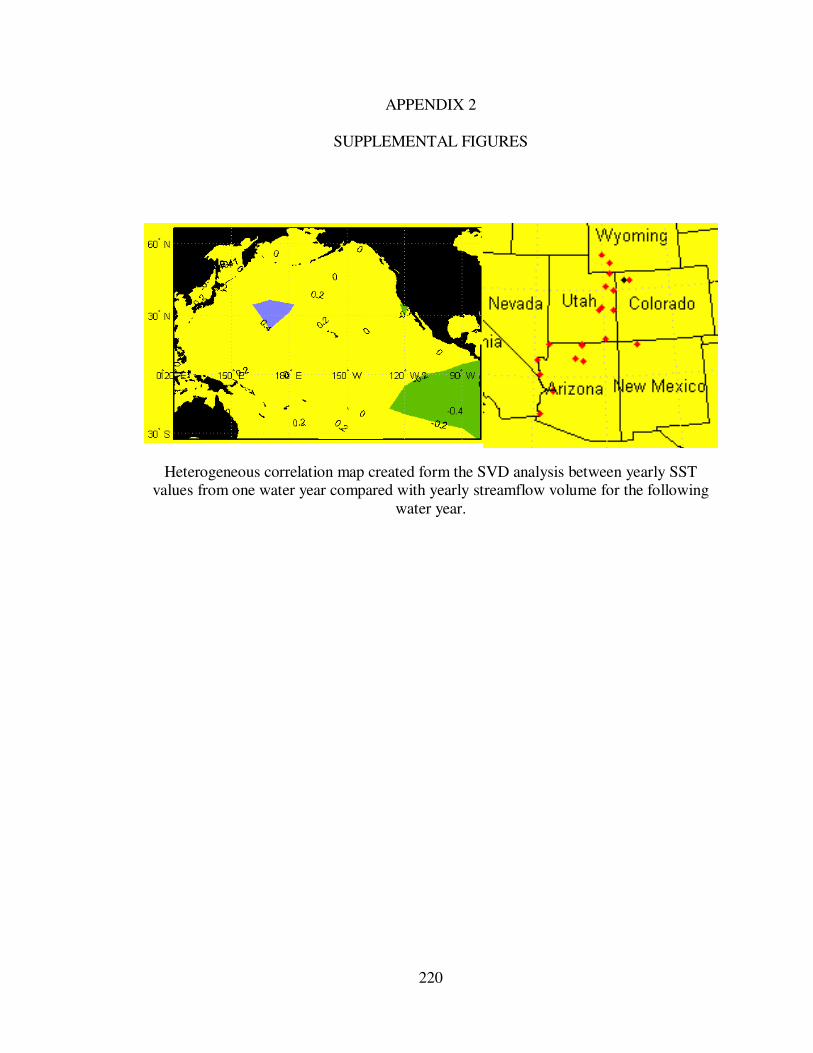
220
APPENDIX 2
SUPPLEMENTAL FIGURES
Heterogeneous correlation map created form the SVD analysis between yearly SST values from one water year compared with yearly streamflow volume for the following
water year.

221
0-Year lag scatter plots of forecast and observed values (gauges 1 – 10)
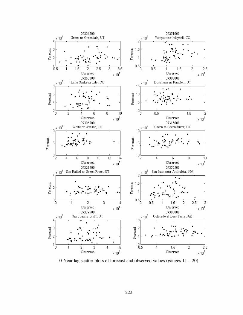
222
0-Year lag scatter plots of forecast and observed values (gauges 11 – 20)
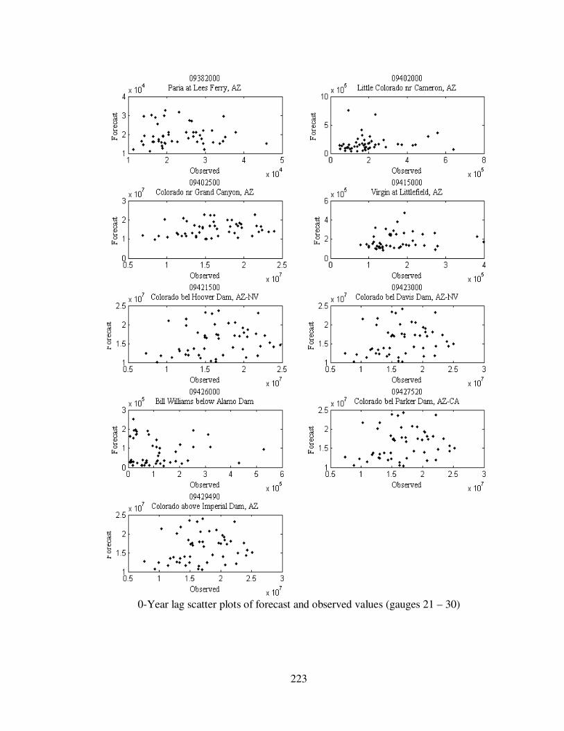
223
0-Year lag scatter plots of forecast and observed values (gauges 21 – 30)
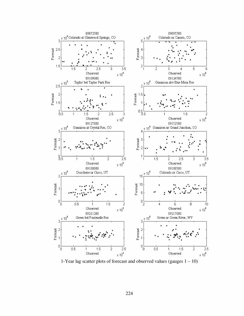
224
1-Year lag scatter plots of forecast and observed values (gauges 1 – 10)

225
1-Year lag scatter plots of forecast and observed values (gauges 11 – 20)

226
1-Year lag scatter plots of forecast and observed values (gauges 21 – 39)

227
2-Year lag scatter plots of forecast and observed values (gauges 1 – 10)

228
2-Year lag scatter plots of forecast and observed values (gauges 11 – 20)

229
2-Year lag scatter plots of forecast and observed values (gauges 21 – 29)
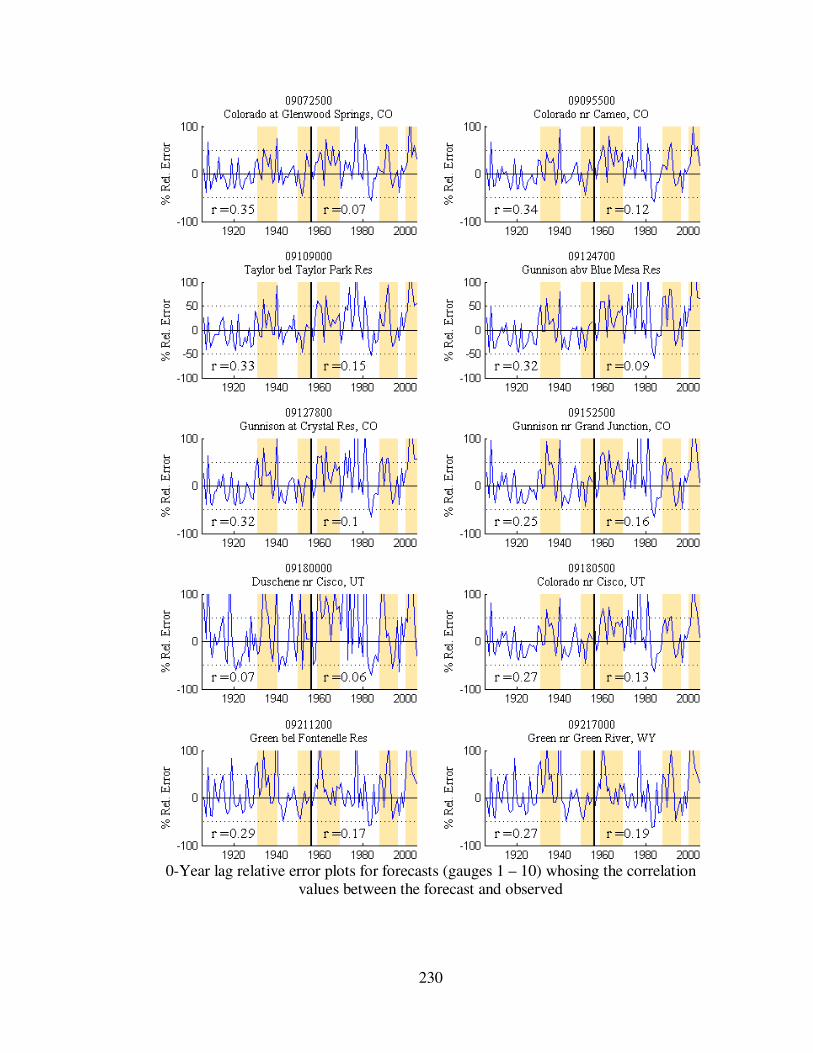
230
0-Year lag relative error plots for forecasts (gauges 1 – 10) whosing the correlation
values between the forecast and observed
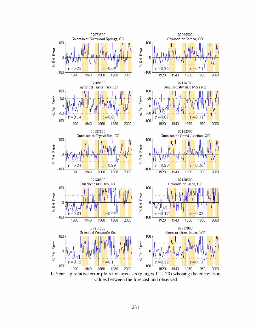
231
0-Year lag relative error plots for forecasts (gauges 11 – 20) whosing the correlation
values between the forecast and observed

232
0-Year lag relative error plots for forecasts (gauges 21 – 29) whosing the correlation
values between the forecast and observed

233
1-Year lag relative error plots for forecasts (gauges 1 – 10) whosing the correlation
values between the forecast and observed
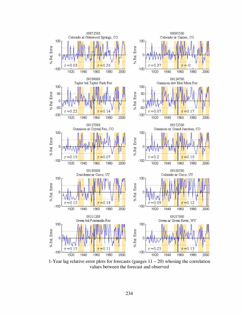
234
1-Year lag relative error plots for forecasts (gauges 11 – 20) whosing the correlation
values between the forecast and observed
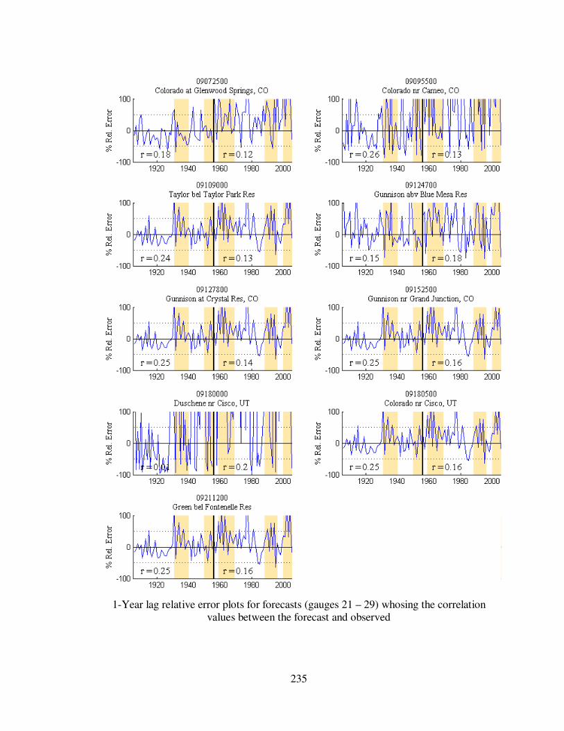
235
1-Year lag relative error plots for forecasts (gauges 21 – 29) whosing the correlation
values between the forecast and observed
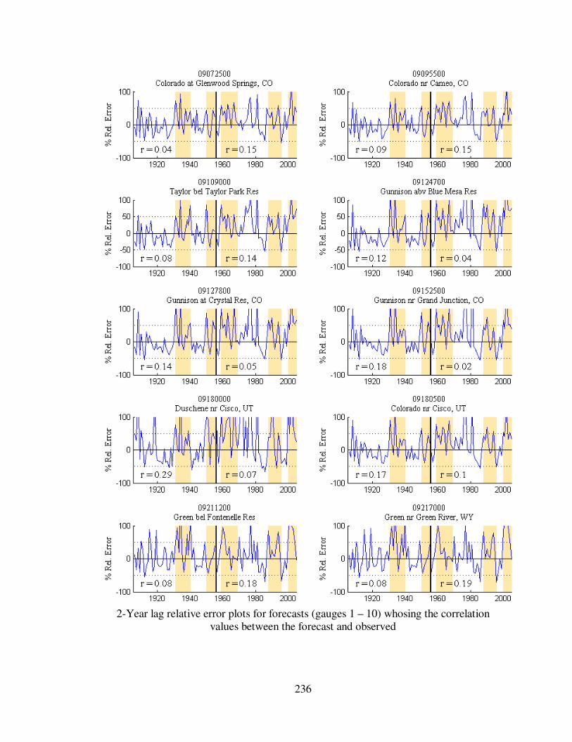
236
2-Year lag relative error plots for forecasts (gauges 1 – 10) whosing the correlation
values between the forecast and observed
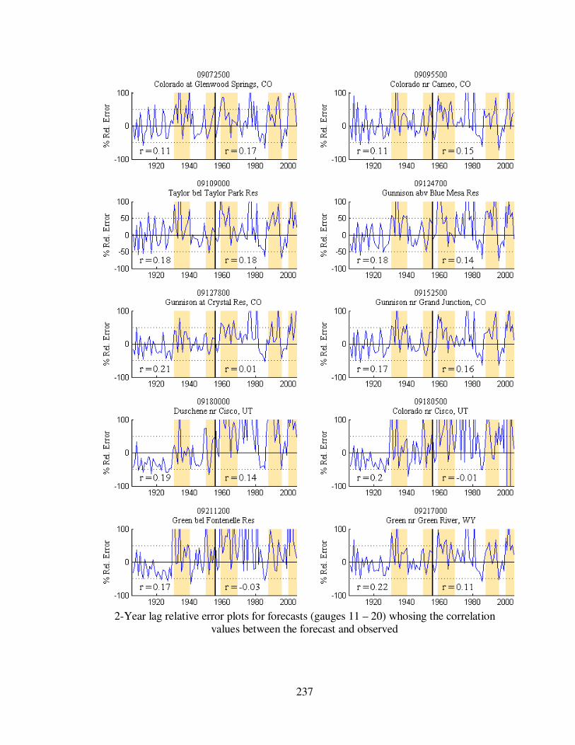
237
2-Year lag relative error plots for forecasts (gauges 11 – 20) whosing the correlation
values between the forecast and observed

238
2-Year lag relative error plots for forecasts (gauges 21 – 29) whosing the correlation
values between the forecast and observed

239
REFERENCES Abramowitz, M. and I.A. Stegun, 1972. Handbook of Mathematical Functions. Dover
Publications, New York
Adam, J.C., A.F. Hamlet, D.P. Lettenmaier, 2009. Implications of global climate change for snowmelt hydrology in the twenty-first century. Hydrological Processes 23(7): 962-97
Alder, H.L., E.B. Roessler 1977. Introduction To Probability And Statistics, Edition: 6, Revised. W H Freeman & Company Limited
An, S.I. 2004. Interdecadal Changes In The El Niño–La Nina Asymmetry. Geophys. Res.
Letters, 31(L23210)
Apipattanavis, S., G.J. McCabe, B. Rajagopalan, and S. Gangopadhyay, 2009. Joint Spatiotemporal Variability of Global Sea Surface Temperatures and Global Palmer Drought Severity Index Values. 22(23): 6251-6267.
Athanasiadis, P.J., J.M. Wallace and J.J. Wettstein, 2010. Patterns of Wintertime Jet Stream Variability and Their Relation to the Storm Tracks. J. Atmos. Sci., 67, 1361–1381.
Aziz, O.A., G.A. Tootle, S.T. Gray, And T.C. Piechota 2010. Identification Of Pacific Ocean Sea Surface Temperature Influences Of Upper Colorado River Basin Snowpack. J Of Water Resour. Res. (In Publication)
Barbe, P., And P. Bertail, 1995. The Weighted Bootstrap. Springer-Verlag, New York, NY
Barnston, A.G., R.E. Livezey 1987. Classification, Seasonality And Persistence Of Low-Frequency Atmospheric Circulation Patterns. Month. Weather Rev.115(6) 1083.
Baughman, R.G., D.M. Fuquay, And P.W. Mielke Jr., 1976. Statistical Analysis Of A Randomized Lightning Modification Experiment. Journal Of Applied Meterology, 15, 790-794.
Beamish, R. J. 1993. Climate And Exceptional Fish Production Off The West Coast Of North America. Can. J. Fish. Aquat. Sci., 50, 2270–2291.
Beebee, R.A. And M. Manga 2004. Variation In The Relationship Between Snowmelt Runoff In Oregon And ENSO And PDO. Journal American Water Resources Association, 40(4):1011-1024.
Bjerknes, J., 1964. Atlantic Air–Sea Interaction. Advances In Geophysics, 10:1–82.
Blackmon, M.L., 1976. A Climatological Spectral Study of the 500 mb Geopotential Height of the Northern Hemisphere. J. of Atmospheric Sciences 33(8):1607-1623.

240
Booker, J.F. 1995. Hydrologic And Economic Impacts Of Drought Under Alternative Policy Responses. Water Resourc. Bull., 31(5), 889-906
Bracken, C., B. Rajagopalan, J. Prairie. 2010. A multisite seasonal ensemble streamflow forecasting technique. Water Resour. Res. 46:3,
Brandon, D.G., 1998. Forecasting Streamflow In The Colorado And Great Basins Using El Niño Indices As Predictors In A Statistical Water Supply Forecast System. Floodplain Management Association, San Diego, CA.
Bretherton, C. S., C. Smith, And J. M. Wallace 1992. An Intercomparison Of Methods For Finding Coupled Patterns In Climate Data, J. Of Climate., 5, 541– 560.
Cayan, D.R., And D.H. Peterson, 1989. The Influence Of North Pacific Atmospheric Circulation On Streamflow In The West. Aspects Of Climate Variability In The Pacific And The Western Americas, American Geophysical Union, Geophysical Monograph Series, 55:375-397.
Cayan, D.R., And R.H. Webb, 1992. El Niño/Southern Oscillation And Streamflow In The Western United States. El Niño: Historical And Paleoclimatic Aspects Of The Southern Oscillation. Cambridge University Press, New York, NY.
Casola, J.H. and J.M. Wallace. 2007. Identifying Weather Regimes in the Wintertime 500-hPa Geopotential Height Field for the Pacific–North American Sector Using a Limited-Contour Clustering Technique. J. of App. Meteorol. and Climatol.
46:10, 1619-1630
Chao, Y., M. Ghil And J.C. Mcwilliams 2000. Pacific Interdecadal Variability In The Century’s Sea Surface Temperatures. Geophys. Res. Lett., 27, 2261-2264.
Chen, T.-C., 1985. Global Water Vapor Flux and Maintenance During FGGE. Mon. Wea.
Rev., 113: 1801-1819.
Cholaw B., J. Liren 1999. The Ocean-Atmosphere Coupled Regimes And East Asian Winter Monsoon (EAWM) Activity. Advances In Atmospheric Sciences 16(1): 91.
Clark, W. G., S. R. Hare, A. M. Parma, P. J. Sullivan And R. J. Trumble 1999. Decadal Changes In Growth And Recruitment Of Pacific Halibut (Hippoglossus Stenolepis). Can. J. Fish. Aquat. Sci., 56, 173–183.
Clark, M. P., M. C. Serreze, And G. J. Mccabe 2001. Historical Effects Of El Niño And La Nina Events On The Seasonal Evolution Of The Montane Snowpack In The Columbia And Colorado River Basins, Water Resour. Res., 37(3), 741–757.
Day, G.A. 1985. Extended Streamflow Forecasting Using NWSRFS J. Of Water Resour
Plng And Mgmt. 111(2) 157 – 170

241
Deser, C., And M. L. Blackmon 1993. Surface Climate Variations Over The North Atlantic Ocean During Winter: 1900–1989. J.Climate, 6:1743–1753.
Dettinger, M.D., D.R. Cayan, H.F. Diaz, and D. M. Meko, 1998. North-South Precipitation Patterns in Western North America on Interrannual-to-Decadal Timescales. J.Clim. 11:3095-3111
Diaz, H.F., And V. Markgraf (Eds.) 1992. El Niño: Historical And Paleoclimatic
Aspects Of The Southern Oscillation. Cambridge University Press, New York, NY
Diaz, H.F., And V. Markgraf (Eds.) 2000. “El Niño And The Southern Oscillation: Multiscale Variability And Global And Regional Impacts” Cambridge University Press, New York, NY
Dijkstra, H.A., L. Raa, M. Schmeits, And J. Gerrits 2006. On The Physics Of The Atlantic Multidecadal Oscillation. Ocean Dynamics 56:36-50
Dima, M., And G.Lohmann 2007. A Hemispheric Mechanism For The Atlantic Multidecadal Oscillation. J. Clim 20, 2706-2719
Dracup, J.A., And E. Kahya, 1992. The Potential For Long-Range Streamflow Forecasting Based On ENSO. Proceedings Of The Sixteenth Annual Climate Diagnostics Workshop, Los Angeles, CA.
Druce, D.J. 2001 Insights From a History of Seasonal Inflow Forecasting With a Conceptual Hydrologic Model. J. Hydrology. 249:102-112
Dugam SS, Kakade SB,Verma RK 1997. Interannual And Long-Term Variability In The North Atlantic Oscillation And Indian Summer Monsoon Rainfall. Theoretical And Applied Climatology 58(1-2): 21.
Durkee JD, J.D. Frye, C.M. Fuhrmann, M.C. Lacke, H.G. Jeong, And T.L. Mote 2008. Effects Of The North Atlantic Oscillation On Precipitation-Type Frequency And Distribution In The Eastern United States. Theoretical And Applied Climatology 94(1-2): 51.
Epstein, E.S. 1969 Stochastic Dynamic Prediction. Tellus, 21:739-759
Efron, B. 1979. Bootsrap Methods: Antoher Look At The Jacknife. Ann. Statist. 7:1-26
Efron, B. 1982. The Jacknife, The Bootsrap, And Other Resampling Plans. CBMS-NSF
Regional Conference Series In Applied Mathematics No. 38. Society For
Industrial And Applied Mathematics. Philadelphia, P.A.
Ely, L. L., Y. Enzel, and D.R. Cayan, 1994. Anamalous North Pacific Atmospheric Circulation and Large Winter Floods in the Southwestern United States, J.
Climate, 7: 977-987.

242
Enfield, D.B., A.M Mestas-Nuñez, And P.J. Trimble, 2001. The Atlantic Multidecadal Oscillation And Its Relation To Rainfall And River Flows In The Continental U.S. Geophysical Research Letters, 28(10):2077-2080.
Faber, B.A. and J.R. Stedinger 2001. Reservoir Optimization Using Sampling SDP With Ensemble Streamflow Prediction (ESP) Forecasts. J. Hydrology.
Frei A, And D.A. Robinson 1999. Northern Hemisphere Snow Extent: Regional Variability 1972-1994. International Journal Of Climatology 19(14): 1535.
Fulp, T.J., Theobald, D.M., Williams, B., And Vickers, B 1991. “Decision Support For Colorado River Operations.” In: Waterpower ’91: A New View Of Hydro
Resources, Proc. Of The Intl. Conf. On Hydropower, New York, NY. 2144-2151
García, J., T. Losada And B. Rodríguez-Fonseca 2006. Modulación De Las Teleconexiones Sobre Europa: Pacífico Y Atlántico Tropical. 5ª Asamblea
Hispano-Portuguesa De Geodesia Y Geofísic, Sevilla 2006.
Garrick, D., K. Jacobs, And G. Garfin. 2008. Models, Assumptions, And Stakeholders: Planning For Water Supply Variability In The Colorado River Basin. JAWRA 44(2), 381-398.
George S.E., M.A. Saunders 2001. North Atlantic Oscillation Impact On Tropical North Atlantic Winter Atmospheric Variability. Geophysical Research Letters 28(6): 1015.
Gerreaud, R.D. And D.S. Battisti 1999: Interannual ENSO And Interdecadal ENSO-Like Variability In The Southern Hemisphere Tropospheric Circulation. J. Clim. 12, 2113-2123.
Gershunov, A., And T.P. Barnett, 1998. Interdecal Modulation Of ENSO Teleconnections. Bulletin Of The American Meteorological Society (79):2715-2725.
Gilmore, A.; Magee, T.; Fulp, T.; And Strzepek, K 2000. Multiobjective Optimization Of The Colorado River. In: Joint Conf. Of Water Resourc. Eng. And Water
Resourc. Plng. And Mgmt. 104(5).
Girardin, M.P. J.C. Tardif, M.D. Flanningan, And Y. Bergeron 2006. Synoptic-Scale Atmospheric Circulation And Boreal Canada Summer Drought Variability Of The Past Three Centuries, J. Clim. 19:1922-1947
Gleeson, T.A. 1961 A Statistical Theory of Meterological Measurements and Predictions. J. of Meteorology. 18:192-198
Gleeson, T.A. 1970. Statistical-dynamical Predictions. J. of Applied Meteorology. 9:333-344

243
Gochis, D.J., L. Brito-Castillo, W.J. Shuttleworth. 2007. Correlations between sea-surface temperatures and warm season streamflow in northwest Mexico. International Journal of Climatology 27(7): 883-901
Goebbert, K.H., L.M. Leslie, 2010. Interannual Variability of Northwest Australian Tropical Cyclones. J. Climate, 23: 4538–4555.
Goldenberg, S.B., C.W. Landsea, A.M. Mestas-Nunez, And W.M. Gray 2001. The Recent Increase In Atlantic Hurricane Activity: Causes And Implications. Science. 293(5529) 474-479.
Grantz, K., B. Rajagopalan, M. Clark, And E. Zagona 2005. A Technique For Incorporating Large-Scale Climate Information In Basin-Scale Ensemble Streamflow Forecasts, Water Resour. Res., 41, W10410, Doi:10.1029/2004WR003467.
Grassi B, G. Redaelli, And G. Visconti 2009. Evidence For Tropical SST Influence On Antarctic Polar Atmospheric Dynamics. Geophysical Research Letters 36(9): L09703.
Gray, S.T., L.J. Graumlich, J.L. Betancourt, And G.T. Pederson 2004. A Tree-Ring Based Reconstruction Of The Atlantic Multidecadal Oscillation Since 1567 A.D. Geophys. Res. Letters. 31(L12205)
Grise, K.M., D.W. J. Thompson, T. Birner. 2010. A Global Survey of Static Stability in the Stratosphere and Upper Troposphere. J. of Clim 23:9, 2275-2292
Hamlet, A.F., And D.P. Lettenmaier, 1999. Columbia River Streamflow Forecasting Based On ENSO And PDO Climate Signals. J. Of Water Res. Plan. And Mgmt., 125(6), 333-341.
Hamlet A.F., D. Huppert, and D.P. Lettenmaier 2002. Economic Value of Long-Lead Streamflow Forecasts for Columbia River Hydropower. J. of Water Resourc. Plng
and Mgmt. 128(2): 91 – 101.
Hanson, K., And C.A. Maul, 1991. Florida Precipitation And The Pacific El Niño, 1895-1989. Florida Scientist 54:160-168.
Hare, S. R., N. J. Mantua And R. C. Francis 1999. Inverse Production Regimes: Alaskan And West Coast Salmon. Fisheries, 24, 6–14.
Harnack, R.P., D.T. Jensen, and J.R.Cermak, 1998. Investigation of upper-air conditions occurring with heavy summer rain in Utah. Int. J. Climatol., 18: 701-723.
Harshburger, B., H. Ye, And J. Dzialoski, 2002. Obervational Evidence Of The Influence Of Pacific Sea Surface Temperatures On Winter Precipitation And Spring Stream Discharge In Idaho. Journal Of Hydrology 264(1-4):157-169.
244
Haylock, M. R., P. D. Jones, R. J. Allan, and T. J. Ansell, 2007. Decadal changes in 1870–2004 Northern Hemisphere winter sea level pressure variability and its relationship with surface temperature. J. of Geophys. Res. 112, D11103
Hidalgo, H.G., 2004. Climate Precursors Of Multidecadal Drought Variability In The Western United States, Journal Of Water Resources Research 40(12).
Hidalgo, H.G., & J.A. Dracup 2003. ENSO & PDO Effects On Hydrclimactic Variations Of The Upper Colorado River Basin. J. Of Hydrometeorology, Vol 4.(1)
Hidalgo, H.G. And J.A. Dracup, 2004. Evidence Of The Signature Of North Pacific Multidecadal Processes On Precipitation And Streamflow Variations In The Upper Colorado River Basin, Pending Publication.
Higuchi K., J. Huang And A. Shabbar 1999. A Wavelet Characterization Of The North Atlantic Oscillation Variation And Its Relationship To The North Atlantic Sea Surface Temperature. International Journal Of Climatology 19(10): 1119.
Hodson, D.L.R., et al. 2009. Climate Impacts Of Recent Multidecadal Changes In Atlantic Ocean Sea Surface Temperature: A Multi-Model Comparison. Clim.
Dynam. 14 Apr 2009.
Holland, G.J. And P.J. Webster 2007. Heightened Tropical Cyclone Activity In The North Atlantic: Natural Variability Or Climate Trend? Phil. Trans. R. Soc. A 15 November 2007 365(1860):2695-2716
Hurell, J.W., 1995. Decedal Trends in the North Atlantic Oscillation: Regional Temperatures and Precipitation. Science. 269:676-679
Ionita M., N. Rimbu, And G. Lohmann 2009. Decadal Variability Of The Elbe River Streamflow. International Journal Of Climatology. Under Review.
Jeong, D, Kim, Y 2005. Rainfall-Runoff Models Using Artificial Neural Networks for Ensemble Streamflow Prediction. Hydrological Processes. 19(19):3819-3835.
Johnstone, J.A. 2010 A quasi-biennial signal in western US hydroclimate and its global teleconnections. Climate Dynamics
Kahya, E., And J.A. Dracup 1993. U.S. Streamflow Patterns In Relation To The El Niño / Southern Oscillation. Journal Of Water Resources Research, 29(8):2491-2503.
Kahya, E., And J.A. Dracup 1994a. The Influences Of Type 1 El Niño And La Niña Events On Streamflows In The Pacific Southwest Of The United States. Journal Of Climate 7(6):965-976.
Kahya, E., And J.A. Dracup 1994b. The Relationships Between U.S. Streamflow And La Niña Events. Journal Of Water Resources Research, 30(7):2133-2141.

245
Kalra, A. and S. Ahmad 2009. Using Oceanic-Atmospheric Oscillations for Long Lead Time Streamflow Forecasting. Water Resourc. Res. 45: W03413
Karcher M, F. Kauker, R. Gerdes, E. Hunke, And J. Zhang 2007. On The Dynamics Of Atlantic Water Circulation In The Arctic Ocean. Journal Of Geophysical
Research. 112(C4): C04S02
Kalnay et al.,1996. “The NCEP/NCAR 40-year Reanalysis Project” Bull. Amer. Meteor. Soc., 77, 437-470
Keenlyside, N.S., et al 2008. Advancing Decadal-Scale Climate Prediction In The North Atlantic Sector. Nature 453:84-88.
Kelley, M.H. And J.A. Gore 2008. Florida River Flow Patterns And The Atlantic Multidecadal Oscillation. River. Res. Applic. 24:598-616
Kerr, R. A., 2000. A North Atlantic Climate Pacemaker For The Centuries. Science, 288:1984-1986.
Kiladis, G.N., And H.F. Diaz 1989. Global Climatic Anomalies Associated With Extremes In The Southern Oscillation. J. Clim 2(1):69-90.
Kim B, S. Moon, L. Riyu, R.H. Kripalani 2002. Teleconnections: Summer Monsoon Over Korea And India. Advances In Atmospheric Sciences 19(4): 665.
Kim, T, J.B. Valdes, B. Nijssen, & D. Roncayolo 2006. Quantification Of Linkages Between Large-Scale Climatic Patterns And Precipitation In The Colorado River Basin” J. Of Hydrology. 321: 173-186
Kim, T., C. Yoo., & J. Ahn 2007. Influence Of Climate Variation On Seasonl Precipitation In The Colorado River Basin” Stochastic Environmental Research
And Risk Assessment, 22(3):411-420
Knight, J.R., R.J. Allan, C.K. Folland, M. Vellinga, And M.E. Mann 2005. A Signature Of Persistent Natural Thermohaline Circulation Cycles In Observed Climate. Geophys. Res. Letters 32(L20708)
Knight, J. R., C. K. Folland, And A. A. Scaife 2006. Climate Impacts Of The Atlantic Multidecadal Oscillation, Geophys. Res. Letters, 33, L17706
Krzysztofowicz, R. 1999. Bayesian Theory of Probabilistic Forecasting Via Deterministic Hydrologic Model. Water Resour. Res. 35(9):2739 - 2750
Krzysztofowicz, R. 2001. The Case for Probabilistic Forecasting in Hydrology. J.
Hydrology. 249: 2 – 9
Kushnir, Y., 1994. Interdecadal Variations in North Atlantic Sea Surface Temperature and Associated Atmospheric Conditions. J. Clim. 7:141-157

246
Kushnir Y., W.A Robinson, P. Chang, And A.W. Robertson 2006. The Physical Basis For Predicting Atlantic Sector Seasonal-To-Interannual Climate Variability. Journal Of Climate 19(23): 5949.
Kvam, P.H. And B. Vidakovic 2007. Nonparametric Statistics With Applications To
Science And Engineering. Hoboken, N.J. Wiley-Interscience, C2007
Lamb, K.W., T.C. Piechota, O.A. Azizz, and G.A. Tootle, 2010. Establishing a Basis for Extending Long-Term Forecasts in the Colorado River Basin. J of Hydrologic Engineering (In Press)
Latif, M And T.P. Barnett 1994. Causes Of Decadal Climate Variability Over The North Pacific And North America. Science 266: 634-637
Leith, C.E. 1974. Theoretical Skill of Monte-Carlo Forecasts. Monthly Weather Review, 102:409-418
Lin, H. 2009. Global Extratropical Response to Diabatic Heating Variability of the Asian Summer Monsoon. J. of the Atmospheric Sciences 66:9, 2697-2713
Lu, R., B. Dong, And H.Ding 2006. Impact Of The Atlantic Multidecadal Oscillation On The Asian Summer Monsoon. Geophys. Res. Letters 33(L24701)
Lundquist, J.D. A.L. Flint. 2006. Onset of Snowmelt and Streamflow in 2004 in the Western United States: How Shading May Affect Spring Streamflow Timing in a Warmer World. J. of Hydrometeorology 7(6): 1199-1217
Macklin M.G. And B.T. Rumsby 2007. Changing Climate And Extreme Floods In The British Uplands. Transactions Of The Institute Of British Geographers 32(2): 168.
Mann, H.B. And D.R. Whitney 1947. On A Test Of Whether One Of Two Random Variables Is Stochastically Larger Than The Other. The Annals Of Mathematical
Statistics. 18(1), 50-60
Mantua, N. J., And S. R. Hare 2002. The Pacific Decadal Oscillation, J. Oceanography, 59(1), 35– 44.
Maurer, E.P., D.P. Lettenmaier, 2003. Predictability of Seasonal Runoff in the Mississippi River Basin, J. Geophys. Res. 108(D16) 8607
Mauer, E.P., D.P. Lettenmaier And N.J. Mantua, 2004. Variability And Potential Sources Of Predictability Of North American Runoff, Pending Publication.
Marshall, J., Y. et al. 2001. North Atlantic Climate Variability: Phenomena, Impacts And Mechanisms. Int J Of Climatology 21:1863-1898
247
Mccabe, G. J. And M. D. Dettinger 1999. Decadal Variations In The Strength Of Enso Teleconnections With Precipitation In The Western United States. Int J Of
Climatology 19 1399-1410 (1999)
Mccabe, G.J. And M.D. Dettinger, 2002. Primary Modes And Predictability Of Year-To-Year Snowpack Variations In The Western United States From Teleconnections With Pacific Ocean Climate. Journal Of Hydrometeorology, 3(1):13-25.
Mccabe, Gregory J., Julio L. Betancourt, And Hugo G. Hidalgo, 2007. Associations Of Decadal To Multidecadal Sea-Surface Temperature Variability With Upper Colorado River Flow. J Of The Amer Water Res. Assoc. 43:183-192.
Mcfarlane, G. And R. J. Beamish 1992. Climatic Influence Linking Copepod Production With Strong Year-Classes In Sablefish, Anaplopoma Fimbria. Can. J. Fish.
Aquat. Sci., 49, 743–753.
Miller, N.L., J. Kim, J.Y. Zhang, J. Oh. 2001. Coupled Precipitation-Streamflow Simulations at the GAME/HUBEX Site: Sixian Basin. J. of the Meteorological Society of Japan 79(5): 985-998
Miller W.D., D.G. Kimmel, And L.W. Harding 2006. Predicting Spring Discharge Of The Susquehanna River From A Winter Synoptic Climatology For The Eastern United States. Water Resources Research 42(5): W05414.
Miller, W.P. and T.C. Piechota 2008. Regional Analysis Of Trend And Step Changes Observed In Hydroclimatic Variables Around The Colorado River Basin. J. Of
Hydrometeorology. 9, 1020.
Milly, C., et al. (2008), Stationary is dead: Whither water management, Science, 318, 573–574.
Minobe, S. 1997. A 50-70 Year Climatic Oscillation Over The North Pacific And North America. Geophys. Re. Lett., 24, 683-686.
Mo, K.C., G.H. White, 1985. Teleconnections in the Southern Hemisphere. Mon. Wea.
Rev., 113: 22–37.
Monahan, A.H., And A. Dai 2004. The Spatial And Temporal Structure Of ENSO Nonlinearity. J. Clim. 17(15):3026-3036.
Morin J, P. Block, B. Rajagopalan, And M. Clark 2008. Identification Of Large Scale Climate Patterns Affecting Snow Variability In The Eastern United States. International Journal Of Climatology 28(3): 315.
Muñoz E., And D. Enfield 2009. The Boreal Spring Variability Of The Intra-Americas Low-Level Jet And Its Relation With Precipitation And Tornadoes In The Eastern United States, Clim. Dynam.

248
Nakamura, H 1996. Year-To-Year And Interdecadal Variability In The Activity Of Intraseasonal Fluctuations In The Northern Hemisphere Wintertime Circulation. Theoretical And Applied Climatology 55(1-4): 19
National Resources Conservation Service (NRCS), National Water And Climate Center, 1997. Southern Oscillation Index Statistical Correlation With Spring Runoff In The Western United States – Report.
Nitta, T. And S. Yamada 1989: Recent Warming Of Tropical Sea Surface Temperatures And Its Relationship To The Northern Hemisphere Circulation. J. Meteor. Soc.
Japan, 67, 375-383.
Oikonomou C., H.A. Flocas, M. Hatzaki, A. Nisantzi, D.N. Asimakopoulos 2010. Relationship Of Extreme Dry Spells In Eastern Mediterranean With Large-Scale Circulation. Theoretical And Applied Climatology 100(1-2): 137
Ottersen G., B. Ãdlandsvik, And H. Loeng 2000. Predicting The Temperature Of The Barents Sea. Fisheries Oceanography 9(2): 121.
Pauluis, O., A. Czaja, R. Korty, 2010. The Global Atmospheric Circulation in Moist Isentropic Coordinates. J. of Climate 23(11): 3077-3093
Patricola, C.M., K.H. Cook. 2009 Northern African climate at the end of the twenty-first century: an integrated application of regional and global climate models. Climate Dynamics
Piechota, T.C., And J.A. Dracup, 1996. Drought And Regional Hydrologic Variation In The United States: Associations With El Niño-Southern Oscillation. Journal Of Water Resources Research, 32(5):1359-1373.
Piechota T.C., And J.A. Dracup, And R.G. Fovell, 1997. Western U.S. Streamflow And Atmospheric Circulation Patterns During El Niño-Southern Oscillation. Journal Of Hydrology, 201:249-271.
Piechota, T.C., F.H.S. Chiew, J.A. Dracup, And T.A. Mcmahon 1998. Seasonal Streamflow Forecasting In Eastern Australia And The El Niño-Southern Oscillation. Journal Of Water Resources Research, 34(11), 3035-3044.
Potts, J.M., C.K. Folland, I.T. Jolliffe, And D. Sexton, 1996. Revised "LEPS" Scores For Assessing Climate Model Simulations And Long-Range Forecasts. J. Climate, 9, 34-53.
Power, S., F. Tseitkin, S. Totrok, B. Lavery, R. Dahni And B. Mcavaney 1997. Australian Temperature, Australian Rainfall And The Southern Oscillation, 1910-1992: Coherent Variability And Recent Changes. Austr. Meteorol. Mag. 47:85-101

249
Power, S., F. Tseitkin, V. Mehta, B. Lavery, S. Torok And N. Holbrook 1999a. Decadal Cliamte Variability In Australia During The Twentieth Century. Int J. Climatol., 19:169-184
Power, S., T. Casey, C. Folland, A. Coleman, And V. Mehta 1999b. Interdecadal Modulation Of The Impact Of ENSO On Australia. Clim. Dyn., 15:319-324
Prohaska, J. 1976. A Technique For Analyzing The Linear Relationships Between Two Meterological Fields. Monthly Weather Review. 104 , 1345 – 1353.
Rajagopalan, B., And U. Lall, 1999. A K-Nearest Neighbor Simulator For Daily Precipitation And Other Weather Variables, J. Of Water. Resour. Res. 35(10):3089-3101
Rajagopalan, B., E. Cook, U. Lall, And B. K. Ray 2000, Spatiotemporal Variability Of ENSO And SST Teleconnections To Summer Drought Over The United States During The Twentieth Century, J. Clim, 13, 4244– 4255.
Rasmussen EM, Wallace JM. 1983. Meteorological Aspects Of The El Niño/Southern Oscillation. Science 222: 1195–1202.
Redmond, K.T., And R.W. Koch, 1991. Surface Climate And Streamflow Variability In The Western United States And Their Relationship To Large-Scale Circulation Indices. Water Resources Research, 27(9):2381-2399.
Richter, I., S.-P. Xie, 2009. Moisture transport from the Atlantic to the Pacific basin and its response to North Atlantic cooling and global warming. Climate Dynamics
Rogers, Jeffery C., 1990. Patterns of Low-Frequency Monthly Sea Level Pressure Variability (1899–1986) and Associated Wave Cyclone Frequencies. J. Climate, 3: 1364–1379.
Rogers, J.C And J.S.M.Coleman 2003. Interactions Between The Atlantic Multidecadal Oscillation, El Niño/Laniña, And The PNA In Winter Mississippi Valley Stream Flow, Geophys. Res. Lett., 30(10):1518
Ropelewski, C.F., And M.S. Halpert, 1986. North American Precipitation And Temperature Patterns Associated With The El Niño / Southern Oscillation. Monthly Weather Review, 114(2):2352-2362.
Ropelewski, C.F., And M.S. Halpert, 1989. Precipitation Patterns Associated With The High Index Phase Of The Southern Oscillation. J. Of Clim. 2:268-284.
Roundy, P.E., L.M. Gribble-Verhagen, 2010. Variations in the Flow of the Global Atmosphere Associated with a Composite Convectively Coupled Oceanic Kelvin Wave. Journal of Climate 23:15, 4192-4201

250
Roundy, P.E., K. MacRitchie, J. Asuma, T. Melino. 2010. Modulation of the Global Atmospheric Circulation by Combined Activity in the Madden–Julian Oscillation and the El Niño–Southern Oscillation during Boreal Winter. Journal of Climate 23:15, 4045-4059
Sangoyomi, T.B., And Harding, B.L. 1995. “Mitigating Impacts Of A Severe Sustained Drought On Colorado River Water Resources.” Water Resour. Bull. 31(5) 925-938
Santos, J. A., J. Corte-Real, U. Ulbrich and J. Palutikof, 2007. European Winter Precipitation Extremes and Large-Scale Circulation: A Coupled Model and its Scenarios. Theor. Appl. Climatol. 87, 85–102
Schlesinger, M.E. And N. Ramankutty 1994. An Oscillation In The Global Climate System Of Period 65–70 Years. Nature 367:723 - 726
Schmidt, N., And E.K. Lipp, J.B. Rose, And M.E. Luther, 2001. ENSO Influences On Seasonal Rainfall And River Discharge In Florida. Journal Of Climate – Notes And Correspondence 14:615-628.
Schuster, R.J. 1989 “The Colorado River Simulation System.” Hydraulic Engineering,
ASCE New York, NY, M. Ports, Ed. 473-478
Serrano Mendoza, E., And B. Rodriguez De Fonseca 2004 Dinámica De La Columna Atmosférica En La Teleconexión Entre Anomalías Superficiales Oceánicas En El Atlántico Subtropical Y La Variabilidad Climática En El Sector Euro-Atlántico. Física De La Tierra, 16:49-59
Shabbar, A., B. Bonsal, And M. Khandekar, 1997. Canadian Precipitation Patterns Associated With The Southern Oscillation. J. Clim. 10, 3016-3027
Shabbar A, And W. Skinner, 2004. Summer Drought Patterns In Canada And The Relationship To Global Sea Surface Temperatures. J. Clim. 17(14): 2866.
Shafer, J.C. and W.J. Steenburgh, 2008. Climatology of Strong Intermountain Cold Fronts, Mon. Wea. Rev., 136:784-807.
Shentsis, I., A. Ben-Zvi 2001 Considering Diversity in Precipitation Variability When Updating Seasonal Flow Forecasts. J. Hydrology 249: 87 - 101
Shuanglin, L., And G.T. Bates 2003 Influence Of The Atlantic Multidecadal Oscillation On The Winter Climate Of East China, Adv. In Atmos. Sci., 24(1):126–135
Shi, X., A.W. Wood, D.P. Lettenmaier, 2008. How Essential is Hydrologic Model Calibration to Seasonal Streamflow Forecasting? J. of Hydrometeorology 9(6): 1350-1363

251
Simpson, J.J., M.D. Dettinger, F.Gehrke, T.J. McIntire, G.L. Hufford, 2004. Hydrologic Scales, Cloud Variability, Remote Sensing, and Models: Implications for Forecasting Snowmelt and Streamflow. Weather and Forecasting 19(2): 251-276
Skinner W.R., A. Shabbar, M.D. Flannigan, And K. Logan 2006 Large Forest Fires In Canada And The Relationship To Global Sea Surface Temperatures. Journal Of
Geophysical Research 111(D14): D14106.
Smith, T.M., And R.W. Reynolds 2003. Extended Reconstruction Of Global Sea Surface Temperatures Based On COADS Data (1854-1997). J. Clim., 16:1495-1510.
Smith, T.M., And R.W. Reynolds, 2004. Improved Extended Reconstruction Of SST (1854-1997). J Of Clim., 17: 2466-2477.
Smith, T.M., R.W. Reynolds, Thomas C. Peterson, and Jay Lawrimore, 2008: Improvements to NOAA's Historical Merged Land-Ocean Surface Temperature Analysis (1880-2006). Journal of Climate,21, 2283-2296.
Soukup, T., O., Aziz, G. Tootle, S. Wulff And T. Piechota 2010. Incorporating Climate Into A Long Lead-Time Non-Parametric Streamflow Forecast. J Of Hydrology (In Press).
Souza Filho, F.A. and U. Lall 2003. Seasonal to Interannual Ensemble Streamflow Forecasts for Ceara, Brazil: Applications of a Multivariate, Semiparametric Algorithm. J. Water Resourc. Res. 39 (11): 1307
Stevens, D. 1986. “Computer Models In Lower Colorado River Operations”. J. Of Water
Resour. Plng. And Mgmt. 112 (3) Pp. 395-408
Sutton R.T. And D.L.R. Hodson, 2005. Atlantic Ocean Forcing Of North American And European Summer Climate. Science, 309:115-118.
Thompson, D.W.J. and J.M. Wallace, 1998. The Arctic Oscillation Signature in the Wintertime Geopotential Height and Temperature Fields, Geophys. Res. Letters, 25(9): 1297-1300. May 1, 1998
Timilsena, J.A., T.C. Piechota, H Hidalgo, G.A. Tootle 2007 “Five Hundred Years Of Hydrological Drought In The Upper Colorado River Basin” J Of Amer. Water Res. Assoc., 43(3): 798-812
Timilsena, J.A., T.C. Piechota, G.A. Tootle, And A.K. Singh 2009. Associations Of Interdecadal/Interannual Climate Variability And Long-Term Colorado River Basin Streamflow. J. Of Hydrology. 365(3-4), 289-301.
Tootle, G.A., And T.C. Piechota, 2004. Suwannee River Long-Range Streamflow Forecasts Based On Seasonal Climate Predictors. Journal Of The American Water
Resources Association, 40(2), 523-532.
252
Tootle, G.A., T.C. Piechota, A.K. Singh 2005. Coupled Oceanic-Atmospheric Variability And US. Streamflow. Water Resour. Res, 41, W12408 Doi:10.1029/2005WR004381
Tootle, G. A., And T. C. Piechota 2006. Relationships Between Pacific And Atlantic Ocean Sea Surface Temperatures And U.S. Streamflow Variability, Water
Resour. Res., W07411, Doi:10.1029/2005WR004184.
Tootle, G.A., A.K. Singh, T.C. Piechota, And I. Farnham 2007. Long Lead-Time Forecasting Of U.S. Streamflow Using Partial Least Squares Regression. J.
Hydrologic Engrg. 12(5):442-451.
Tootle, G.T. et al, 2009. 2009-2010 El Niño: Hydrologic Relief For Parts Of The U.S.?. EOS Transactions, 90(50), 481-292.
Trenberth, K.E. 1990. Recent Observed Interdecadal Climate Changes In The Northern Hemispheric. Bull Amer. Meteor Soc., 71, 988-993.
Trenberth, K.E. And J.W. Hurell, 1994. Decadal Atmosphere-Ocean Variations In The Pacific. Clim. Dyn., 9, 303-319
Trenberth, K.E. And D.J.Shea 2006 Atlantic Hurricanes And Natural Variability In 2005. Geophys. Res. Letters 33(L12704)
Twine, T.E., C.J. Kucharik, J.A. Foley. 2005. Effects of El Niño–Southern Oscillation on the Climate, Water Balance, and Streamflow of the Mississippi River Basin. J. of Climate 18(22): 4840-4861
Ukita J., et al. 2007. Northern Hemisphere Sea Ice Variability: Lag Structure And Its Implications. Tellus A 59(2): 261.
Van Loon, H. And J.C. Rogers 1978. The Seesaw In Winter Temperatures Between Greenland And Northern Europe. Part I: General Description. Month. Weath.
Rev. 106(3):296-310
Visbeck, M., et al 2002. The Ocean’s Response To North Atlantic Oscillation Variability. The North Atlantic Oscillation: Climatic Significance And Environmental Impact, Geophys. Monogr., 134:113–145.
Walker, G.T. 1923. Correlation Inseasonal Variations Of Weather. Part VIII: A Preliminary Study Of World Weather. Memoirs Of The Indian Meteorological
Department, 24:75-131
Walker, G.T. And E.W. Bliss 1932. World Weather V. Memoirs Of The Royal
Meteorological Society 4:53-84.
Wallace, J.M. and D.S. Gutzler, 1981. Teleconnections in the Geopotential Height Field During the Northern Hemisphere Winter, Mon Wea. Rev. 109:784-812

253
Wallace, J. M., D. S. Gutzler, And C. S. Bretheron 1992, Singular Value Decomposition Of Wintertime Sea Surface Temperature And 500-Mb Height Anomalies, J. Clim., 5, 561–576.
Wang, H. And M. Ting 2000 Covariabilities Of Winter U.S. Precipitation And Pacific Sea Surface Temperatures. J. Clim Oct, 3711-3719.
Wang, S., R. R. Gillies, J. Jin, and L. E. Hipps, 2009. Recent Rainfall Cycle in the Intermountain Region as a Quadrature Amplitude Modulation From the Pacific Decadal Oscillation. Geophys Res Letters 36, L02705.
Wang, S., L.E. Hipps, R.R. Gillies, X. Jiang, A.L. Moller, 2010a. Circumglobal teleconnection and early summer rainfall in the US Intermountain West. Theoretical and Applied Climatology, DOI: 10.1007/s00704-010-0260-4
Wang, S., R. R. Gillies, J. Jin, and L. E. Hipps, 2010b. “Coherence Between the Great Salt Lake Level and the Pacific Quasi-Decadal Oscillation. J. Climate, 23, 2161-2177.
Wang, S., R. R. Gillies, L. E. Hipps, and J. Jin, 2010c. A Transition-Phase Teleconnection of the Pacific Quasi-Decadal Oscillation. Clim Dyn. DOI: 10.1007/s00382-009-0722-5
Ward M.N., Folland C.K. 1991. Prediction Of Seasonal Rainfall In The North Nordeste Of Brazil Using Eigenvectors Of Sea-Surface Temperature. International Journal
Of Climatology 11: 711–743.
Werner, K., D. Brandon, M. Clark, S. Gangopadhyay 2004. Climate Index Weighting Schemes For NWS ESP-Based Seasonal Volume Forecasts. J. Hydrometerology. 5, 1076-1090.
Wilcoxon, F. 1945. “Individual Comparisons By Ranking Methods.” Biometrics
Bulletin 1(6), 80-83
Wilks, D.S. 2006. Statistical Methods In The Atmospheric Sciences, Academic Press (Elsevier) Burlington, MA
Willmott, C.J., K. Matsuura, 2005. Advantages of the mean absolute error (MAE) over the root mean square error (RMSE) in assessing average model performance. Clim. Res. 30:79-82
Wu W, R.E. Dickinson, H. Wang, Y. Liu, And M. Shaikh 2007. Covariabilities Of Spring Soil Moisture And Summertime United States Precipitation In A Climate Simulation. International Journal Of Climatology 27(4): 429
Wu, B., R. Zhang, B. Wang, and R. D’Arrigo, 2009. On the association between spring Arctic sea ice concentration and Chinese summer rainfall. Geophys. Res. Ltrs, 36, L09501

254
Xue Y., S. Sun, K. Lau, J. Ji, I. Poccard, R. Zhang, H. Kang, G. Wu, J.C. Schaake, And J.Y. Zhang 2005. Multiscale Variability Of The River Runoff System In China And Its Long-Term Link To Precipitation And Sea Surface Temperature. Journal Of Hydrometeorology 6(4): 550.
Yang, S., K.-M. Lau, and K.-M. Kim, 2002. Variations of the East Asian Jet Stream and Asian-Pacific –American Winter Cliamte Anomalies. J. Climate, 15(3):306-325
Yang Q. (2009). Impact Of The Indian Ocean Subtropical Dipole On The Precipitation Of East China During Winter Monsoons. Journal Of Geophysical Research 114(D14): D14110.
Yarnal B., And H. F. Diaz, 1986. Relationships Between Extremes Of The Southern Oscillation And The Winter Climate Of The Anglo-American Pacific Coast. Journal Of Climatology, 6, 197-219.
Yu, B. 2007. The Pacific–North American pattern associated diabatic heating and its relationship to ENSO. Atmospheric Science Letters, 8: 107–112. doi: 10.1002/asl.160
Yuan, X. and C. Li, 2008. Climate Modes in Southern High Latitudes and Their Impacts on Antarctic Sea Ice. J. of Geophys. Res. Ltrs. 113. C06S91
Zagona, E.A., T.J. Fulp, R. Shane, T. Magee, And H.M. Goranflo 2001. Riverware: A Generalized Tool For Complex Reservoir System Modelling.” JAWRA. 37(4) 913-929
Zhang, Y., K.R. Sperber, J.S. Boyle 1997a. Climatology and Interannual Variation of the East Asian Winter Monsoon: Results from the 1979-95 NCEP/NCAR Reannalysis. Monthly Weather Review. Oct 1997
Zhang, Y., J.M. Wallace, and D.S. Battisti, 1997b. ENSO-like Interdecadal Variability: 1900-93, J. Clim., 10:1004-1020..
Zhang, R. And T.L. Delworth 2006. Impact Of Atlantic Multidecadal Oscillations On India/Sahel Rainfall And Atlantic Hurricanes. Geophys. Res. Letters 33(L17712)
Zhang, R., And T. L. Delworth 2007. Impact Of The Atlantic Multidecadal Oscillation On North Pacific Climate Variability, Geophys. Res. Lett., 34(L23708)
Zhao, M., I.M. Held, S. Lin, G.A. Vecchi. 2009. Simulations of Global Hurricane Climatology, Interannual Variability, and Response to Global Warming Using a 50-km Resolution GCM. J. of Climate 22:24, 6653-6678
Zhifang F, And J.M. Wallace 1993. The Relationship Between The Wintertime Blocking Over Greenland And The Sea Ice Distribution Over North Atlantic. Advances In
Atmospheric Sciences 10(4): 453.

255
Zorn, M.R., And P.R. Waylen, 1997. Seasonal Response Of Mean Monthly Streamflow To El Niño / Southern Oscillation In North Central Florida. Professional Geographer 49:51-62.

256
VITA
Graduate College University of Nevada, Las Vegas
Kenneth W. Lamb
Degrees: Bachelor of Science, Civil Engineering, 2003 University of Nevada, Las Vegas Masters in Civil Engineering, 2007 Norwich University Publications: A Basis for Extending Long-Term Streamflow Forecasts in the Colorado River. Journal of Hydrologic Engineering, in press, 2010. Dissertation Title: Improving Ensemble Streamflow Prediction Using Interdecadal/Interannual Climate Variability Dissertation Examination Committee: Chairperson, Thomas C. Piechota, Ph.D, P.E. Committee Member, Jacimaria Batista, Ph.D, P.E. Committee Member, Sajjad Ahmad, Ph.D. Committee Member, Ashok K. Singh, Ph.D Graduate Faculty Representative, Susanna Priest, Ph.D.