improving backfilling by using machine learning to predict
TRANSCRIPT
HAL Id: hal-01221186https://hal.archives-ouvertes.fr/hal-01221186
Submitted on 27 Oct 2015
HAL is a multi-disciplinary open accessarchive for the deposit and dissemination of sci-entific research documents, whether they are pub-lished or not. The documents may come fromteaching and research institutions in France orabroad, or from public or private research centers.
L’archive ouverte pluridisciplinaire HAL, estdestinée au dépôt et à la diffusion de documentsscientifiques de niveau recherche, publiés ou non,émanant des établissements d’enseignement et derecherche français ou étrangers, des laboratoirespublics ou privés.
Copyright
Improving Backfilling by using Machine Learning topredict Running Times
Eric Gaussier, David Glesser, Valentin Reis, Denis Trystram
To cite this version:Eric Gaussier, David Glesser, Valentin Reis, Denis Trystram. Improving Backfilling by using MachineLearning to predict Running Times. SuperComputing 2015, Nov 2015, Austin, TX, United States.�10.1145/2807591.2807646�. �hal-01221186�
Improving Backfilling by using Machine Learning topredict Running Times
Eric GaussierUniversity Grenoble-Alpes,
LIG, [email protected]
David GlesserBULL – HPC division,
Grenoble, [email protected]
Valentin ReisUniversity Grenoble-Alpes,
LIG, [email protected]
Denis TrystramUniversity Grenoble-Alpes,
LIG, [email protected]
ABSTRACTThe job management system is the HPC middleware re-sponsible for distributing computing power to applications.While such systems generate an ever increasing amount ofdata, they are characterized by uncertainties on some pa-rameters like the job running times. The question raised inthis work is: To what extent is it possible/useful to take intoaccount predictions on the job running times for improvingthe global scheduling?
We present a comprehensive study for answering this ques-tion assuming the popular EASY backfilling policy. Moreprecisely, we rely on some classical methods in machinelearning and propose new cost functions well-adapted to theproblem. Then, we assess our proposed solutions throughintensive simulations using several production logs. Finally,we propose a new scheduling algorithm that outperforms thepopular EASY backfilling algorithm by 28% considering theaverage bounded slowdown objective.
KeywordsHigh Performance Computing, Running Time Estimation,Scheduling, Machine Learning
1. INTRODUCTION
1.1 ContextLarge scale high performance computing (HPC) platforms
are becoming increasingly complex. There exists a broadrange and variety of HPC architectures and platforms. Asa consequence, the job management system (which is themiddleware responsible for managing and scheduling jobs)should be adapted to deal with this complexity. Determiningefficient allocation and scheduling strategies that can dealwith complex systems and adapt to their evolutions is a
ACM ISBN 978-1-4503-3723-6/15/11. . . $15.00
DOI: http://dx.doi.org/10.1145/2807591.2807646
strategic and difficult challenge.More and more data are produced in such systems by
monitoring the platform (CPU usage, I/O traffic, energyconsumption, etc.), by the job management system (i.e., thecharacteristics of the jobs to be executed and those whichhave already been executed) and by analytics at the appli-cation level (parameters, results and temporary results). Allthis data is most of the time ignored by the actual systemsfor scheduling jobs.
The technologies and methods studied in the field of bigdata (including Machine Learning) could and must be usedfor scheduling jobs in the new HPC platforms.
For instance, and this will be the focus of this paper, therunning time of a given job on a specific HPC platform isusually not known in advance and moreover, it depends onthe context (characteristics of the other jobs, global load,etc.). In practice, most job management systems ask theusers for an upper bound on the job running time, threat-ening to kill it if it exceeds this requested value. This leadsto very bad estimates of the running times given by theusers [23]. A precise knowledge of the running times is evenmore important since the algorithms used in most of thesesystems assume that this value is perfectly known. Thus, itis crucial to determine how to estimate the running timesin order to improve scheduling. We believe that there is ahuge potential gain in studying this question more deeplyand provide more efficient scheduling mechanisms.
Obviously, the job running time is not the only parameterimpacted by uncertainties. We focus on it as a proof ofconcept in order to show that it is possible to improve thescheduling performances for popular FCFS-BF (First ComeFirst Serve with Backfilling) batch scheduling policy. Theanalysis provided on this work can be extended easily toother scheduling policies.
1.2 ContributionsThe main question addressed in this work is to determine
to what extent predictions of the running times may helpfor obtaining a better schedule. For this purpose, we rely onon-line regression methods and consider a family of loss (orcost) functions that are used to learn the prediction model.Then, we show how to use the predictions obtained by im-proving popular scheduling algorithms. Finally, we performan experimental evaluation of the proposed new algorithmsusing several actual log datas on various platforms. The re-
sults show an average gain of 28% compared to the classicalEASY policy (with a maximum of 86%) and 11% in averagecompared to EASY++.
1.3 ContentWe start by describing the problem in Section 2. Then,
we present and discuss in Section 3 the main existing ap-proaches studied so far in parallel processing field for pre-dicting running times and their use in scheduling. Section 4recalls the main prediction approaches in machine learn-ing and presents an original method for estimate the run-ning time of the jobs based on linear regression. Then, wepresent the studied scheduling algorithms and their adapta-tion to predictive techniques in Section 5. Section 6 reportsthe simulations done with actual log data. They show thatsome combinations of prediction and scheduling algorithmsimprove the system performances.
2. PROBLEM DESCRIPTION
2.1 Job managementWe are interested in this work in scheduling jobs in HPC
platforms. The application developers (or users) submittheir jobs in a centralized waiting queue. The job manage-ment system aims at determining a suitable allocation forthe jobs, which all compete against each other for the avail-able computing resources. In most HPC centers, these usersare requested to provide some information about their appli-cations in order to help the system to take better decisions.In particular, it is expected that they give an estimation ofthe running times. As a job is killed if its actual runningtime is greater than its requested running time, users tendto significantly increase the duration estimates [23].
Most available open-source and commercial job manage-ment systems use an heuristic approach inspired by backfill-ing algorithms. The job priority is determined according tothe arrival times of the jobs. Then, the backfilling mecha-nism allows a job to run before another job with a highestpriority only if it does not delay it. There exist several vari-ants of this algorithm, like conservative backfilling [14] andEASY backfilling [9]. In the former, the job allocation iscompletely recomputed at each new event (job arrival or jobcompletion) while in the second, the process is purely on-lineavoiding costly recomputations.
SLURM is the most popular job management system [25].In the last release of the TOP500 ranking in November 2014,SLURM was performing job management in six of the tenmost powerful systems, including the number one. It usesEASY backfilling and includes the possibility to sort thewaiting jobs according to various priorities (like by increas-ing age, size or share factors, etc.). Other job managementsystems including MOAB [12], TORQUE [22], PBSpro [17]or LSF [11] are built upon the same approach with theirown specificities. A review on job schedulers can be foundin Georgiou [7].
We focus on EASY backfilling as a basic mechanism forassessing our approach. In the remaining of the paper, thecorresponding policy will be denoted in short by EASY.
2.2 Dealing with uncertaintiesThe objective of this section is to show by some simu-
lations on actual data that using good running time pre-
Table 1: AVEbsld performances of EASY (using re-quested times) and EASY-Clairvoyant (using actualrunning times). Values between parentheses showthe corresponding decrease in AVEbsld.
Log EASY EASY-Clairvoyant
KTH-SP2 92.6 71.7 (22%)
CTC-SP2 49.6 37.2 (25%)
SDSC-SP2 87.9 70.5 (19%)
SDSC-BLUE 36.5 30.6 (16%)
Curie 202.1 69.9 (65%)
Metacentrum 97.6 81.7 (16%)
dictions significantly improves the scheduling performances.First, let us clarify the vocabulary: a job is over-predicted ifits predicted running time is greater than the actual runningtime. Similarly, a job is under-predicted when the predictedrunning time is lower than the actual running time.
Table 1 reports the comparison of simulations based onthe testbed detailed in Section 6. Each log runs with EASY,first with the original user’s requested running times, thenwith the actual running times (as if the users were entirelyclairvoyant). The metric used for comparison, AVEbsld isdescribed in Subsection 5.3.
The results reported in Table 1 emphasize that clairvoyantsimulations are in average 27% better than simulations us-ing the original requested running times. As running timesare shorter in the clairvoyant case, more jobs can be back-filled and thus, the performances are improved. Takinginto account actual running time values always improves thescheduling performances, thus accurate running time esti-mates are crucial for reaching good performances.
2.3 Formulation of the problemThe problem studied in this work is to execute a set of
concurrent parallel jobs with rigid resource requirements (itmeans that the number of resources required by a job isknown in advance) on a HPC platform represented by a poolof m identical resources (we do not assume any particularinterconnection topology). The jobs are submitted over time(on-line).
There are n independent jobs (indexed by integers), wherejob j has the following characteristics:
• Submission date rj (sometimes called release date);
• Resource requirement qj (processor count);
• Actual running time pj (sometimes called processingtime);
• Requested running time pj , which is an upper boundon pj ;
• Additional data that has no direct impact on the phys-ical description of the job (e.g. the time of the daywhen the job is submitted or the executable name).This data may be used to learn about jobs, users andthe system.
The resource requirement qj of a job is known when the jobis submitted at time rj , while the running time pj is given
as an estimate. Its actual value is only known a posterioriwhen the job really completes.
The problem is to design several algorithms that predictthe running times in order to provide good scheduling per-formances.
3. RELATED WORK
3.1 PredictionHistorically, job running time prediction has been first
attempted [8] by categorizing the jobs according to a prede-fined set of rules. Then, statistics based on such job’s cat-egory are used to generate a prediction. In this approach,called Templates, a partitioning into templates has to beprovided by the job management system or the system ad-ministrator. It can be seen as an ancestor of tree-basedregression models in which the binning has to be obtainedtrough statistical analysis of the specific system and popula-tion and/or discussion with a domain expert. The techniquewas subsequently adapted [21] using a more automatic way(a genetic algorithm evolving template attributes) to gen-erate the rules. These works used minimal, high-level in-formation about jobs similar to what can be found in HPClogs.
There exist other works that use more specialized meth-ods, but require the modeling of the jobs. For instance,Schopf et al. predict running time of applications by ana-lyzing their functional structure [20]. An another exampleis the method developed by Mendes et al. which performsstatic analysis of the applications [13].
A later survey [10] evaluates the use of more recent su-pervised learning tools. This work focuses on two scientificapplications and uses in-depth information about both thejobs (e.g. input parameters) and the machines (e.g. diskspeed). A closely related paper by Duan et al. [3] proposesan hybrid Bayesian-neural network approach to dynamicallymodel and predict the running time of scientific applications.It uses in-depth information about jobs and their environ-ment as well.
All these previous approaches assume jobs and their run-ning times to be identically distributed and independent(i.i.d.), and therefore, they do not leverage dependencies be-tween job submissions. A stochastic model [15] has been pro-posed for predicting job running time distributions. By op-position to the previous studies which only used job descrip-tions, this technique only relies on historical running timeinformation. It treats successive running times of a givenuser as the observations of a Hidden Markov Model [18],and hence it does not use the hypothesis that job submis-sions would be i.i.d..
3.2 Scheduling based on PredictionsThere are only a few methods for performing scheduling
using predictive techniques.The Hidden Markov Model used in [15] is a probabilistic
generative model, and as such it is possible to easily obtainthe conditional distribution of the running time of a job. Asa consequence, it is possible to design scheduling algorithmsthat use job running time distributions as an input [16].
The most relevant work for scheduling jobs on large paral-lel systems using predictions is [24], in which the average ofthe two last available running times of the job’s user is usedas a prediction. It leads to surprisingly good results given its
simplicity. This work also introduces an improved version ofEASY: EASY++. This algorithm use the predicted valuefor the backfilling. The waiting jobs are considered by theirorder of arrival, but during the backfilling phase jobs aresorted shortest first. They also introduce a correction mech-anism: when the the prediction technique under-estimates arunning time, a new estimation of the running time has tobe obtained. The proposed correction mechanism is simple:the authors add a fixed amount of time from a predefinedlist of values each time they under-estimate.
To the best of our knowledge, there is no other work thatrelies on state-of-the-art machine learning methodology forrunning time prediction and evaluates the resulting schedul-ing. In the following two sections, we present prediction andscheduling mechanisms.
4. PREDICTION METHODWe first outline in this section the characteristics that
the prediction method should have, prior to describing ourapproach in detail.
4.1 RationaleLet us first argue that an approach based on machine
learning for predicting the running times of jobs should havethe following characteristics:
It should be based on minimal information. In hopethat results extend well to new HPC systems and beusable in mainstream job management system, a learning-based system should prove its effectiveness on minimaljob descriptions. In this light, one reasonable approachis to use information of the Standard Workload Format(SWF ) [5].
It should work on-line. This is motivated by previous stu-dies which emphasize that dependencies between jobrunning times are so far from being i.i.d. that two suc-cessive running times [24] are enough to predict run-ning time with good accuracy. Therefore, an algorithmbased on batches (which re-approximates the learnedconcept once every k jobs, where k � 1) should notbe favored.
It should use both job description and system historyUnlike previous studies that either assume jobs to betemporally independent or rely exclusively on runningtime locality [15], a holistic approach should leverageboth job descriptions and temporal dependencies.
It should be robust to noise. Because HPC jobs can havean erratic behavior (e.g. they may fail or hang-up),the data one is relying on will be noisy. The learn-ing algorithm should be robust to this noise and avoidoverfitting.
It should accept an arbitrary loss function. Attemptingto minimize the cumulative loss of an arbitrary func-tion allows for a ”declarative” statement of the harmincurred by a misprediction. This last aspect is moti-vated by the intuition that an inaccurate prediction ofa job’s running time would not harm the scheduling inan identical way depending on the job’s characteristicsand the direction of the error. This will be explored
in detail in the next Subsection. Arbitrary loss func-tions generally pose computational limitations, and inpractice convex loss functions are often used.
We now turn to the description of the prediction method.
4.2 A new prediction approachA job j is represented by a vector1 xj ∈ Rn where n is
the number of features of the model. The features which wefeed the algorithm with are described in Table 2. These fea-tures are taken from various sources of information, such asthe job’s description (pj and qj). Others are taken from his-
torical information (e.g. p(k)j−1) and some are taken from the
current state of the system (e.g. Jobs Currently Running).Additionally, some features are taken from the environment(e.g. Time of the day).
The prediction is achieved via a `2-regularized polynomialmodel. This choice is motivated by the availability of highlyrobust algorithms to fit on-line linear regression models [19],even in the presence of an adversary scaling of the features.The `2 norm regularizer is used to prevent the quadraticmodel from overfitting and the polynomial representation(here of degree 2) to take into account dependencies betweenfeatures. The regression function is:
f(w,x) = wᵀΦ(x) w ∈ R1+2n+(n2) (1)
where the wi are the parameters (to be learned) of themodel, and Φ is a vector of basis functions:
Φ(x) = (1, x1, · · · , xn, x1x2, · · · , xkxl, · · · , xn−1xn)ᵀ
Denoting the actual running time of job j by pj , the cumu-lative loss for up to the N -th already-processed job is2:
N∑j=1
L(xj , f(xj), pj)
where L(x, f(x), y) is the loss function associated with pre-dicting a value of f(x) in the case where the actual runningtime is y. The regression problem finally takes the form:
arg minw
N∑j=1
L(xj ,wᵀΦ(xj), pj) + λ||w||2 (2)
where λ is the regularization parameter. Once w has beenlearned, new running times are predicted through Equa-tion (1).
The choice of the loss function is crucial and not straight-forward here as the impact of a bad prediction on the run-ning time varies from job to job as well as from the directionof the error (over- or under-prediction). Indeed, schedulingalgorithms behave differently with respect to under-predictionand over-prediction: in the case of an under-prediction, a de-structive effect on the planned schedule can happen, whilean over-prediction never makes a planned schedule feasiblebut may imply unused resources. This suggests that oneshould rely on asymmetrical losses, that can be based on
1As common in machine learning, we use bold letters todenote vectors and standard letters for scalars.2Note that one can also consider the k latest jobs or weighdifferently the jobs to favor recent ones. These variants arestraightforward to consider from the framework developedhere.
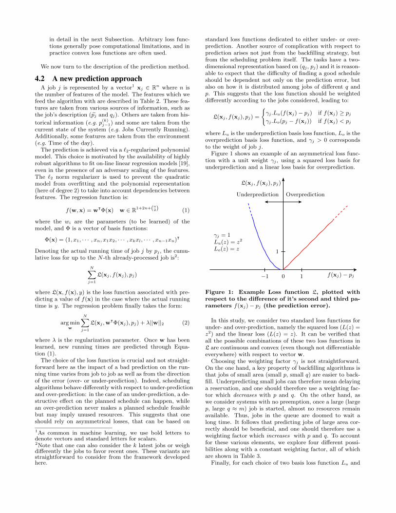
standard loss functions dedicated to either under- or over-prediction. Another source of complication with respect toprediction arises not just from the backfilling strategy, butfrom the scheduling problem itself. The tasks have a two-dimensional representation based on (qj , pj) and it is reason-able to expect that the difficulty of finding a good scheduleshould be dependent not only on the prediction error, butalso on how it is distributed among jobs of different q andp. This suggests that the loss function should be weighteddifferently according to the jobs considered, leading to:
L(xj , f(xj), pj) =
{γj .Lu(f(xj)− pj) if f(xj) ≥ pjγj .Lo(pj − f(xj)) if f(xj) < pj
where Lu is the underprediction basis loss function, Lo is theoverprediction basis loss function, and γj > 0 correspondsto the weight of job j.
Figure 1 shows an example of an asymmetrical loss func-tion with a unit weight γj , using a squared loss basis forunderprediction and a linear loss basis for overprediction.
f(xj)− pj
L(xj , f(xj), pj)
OverpredictionUnderprediction
0
1
1−1
γj = 1Lu(z) = z2
Lo(z) = z
Figure 1: Example Loss function L, plotted withrespect to the difference of it’s second and third pa-rameters f(xj)− pj (the prediction error).
In this study, we consider two standard loss functions forunder- and over-prediction, namely the squared loss (L(z) =z2) and the linear loss (L(z) = z). It can be verified thatall the possible combinations of these two loss functions inL are continuous and convex (even though not differentiableeverywhere) with respect to vector w.
Choosing the weighting factor γj is not straightforward.On the one hand, a key property of backfilling algorithms isthat jobs of small area (small p, small q) are easier to back-fill. Underpredicting small jobs can therefore mean delayinga reservation, and one should therefore use a weighting fac-tor which decreases with p and q. On the other hand, aswe consider systems with no preemption, once a large (largep, large q ≈ m) job is started, almost no resources remainavailable. Thus, jobs in the queue are doomed to wait along time. It follows that predicting jobs of large area cor-rectly should be beneficial, and one should therefore use aweighting factor which increases with p and q. To accountfor these various elements, we explore four different possi-bilities along with a constant weighting factor, all of whichare shown in Table 3.
Finally, for each choice of two basis loss function Lu and
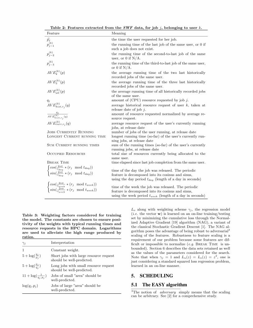
Table 2: Features extracted from the SWF data, for job j, belonging to user k.
Feature Meaning
pj the time the user requested for her job.
p(k)j−1 the running time of the last job of the same user, or 0 if
such a job does not exist.
p(k)j−2 the running time of the second-to-last job of the same
user, or 0 if N/A.
p(k)j−3 the running time of the third-to-last job of the same user,
or 0 if N/A.
AV E(k)2 (p) the average running time of the two last historically
recorded jobs of the same user.
AV E(k)3 (p) the average running time of the three last historically
recorded jobs of the same user.
AV E(k)all (p) the average running time of all historically recorded jobs
of the same user.qj amount of (CPU) resource requested by job j.
AV E(k)hist,rj
(q) average historical resource request of user k, taken atrelease date of job j.
qj
AV E(k)hist,rj
(q)amount of resource requested normalized by average re-source request.
AV E(k)curr,rj (q) average resource request of the user’s currently running
jobs, at release dateJobs Currently Running number of jobs of the user running, at release dateLongest Current running time longest running time (so-far) of the user’s currently run-
ning jobs, at release dateSum Current running times sum of the running times (so-far) of the user’s currently
running jobs, at release dateOccupied Resources total size of resources currently being allocated to the
same user.Break Time time elapsed since last job completion from the same user.{cos( 2∗π
tday∗ (rj mod tday))
sin( 2∗πtday∗ (rj mod tday))
time of the day the job was released. The periodicfeature is decomposed into its cosinus and sinus,using the day period tday (length of a day in seconds){
cos( 2∗πtweek
∗ (rj mod tweek))
sin( 2∗πtweek
∗ (rj mod tweek))time of the week the job was released. The periodicfeature is decomposed into its cosinus and sinus,using the week period tweek (length of a day in seconds)
Table 3: Weighting factors considered for trainingthe model. The constants are chosen to ensure posi-tivity of the weights with typical running times andresource requests in the HPC domain. Logarithmsare used to alleviate the high range produced byratios.
γj Interpretation
1 Constant weight.
5 + log(qjpj
) Short jobs with large resource requestshould be well-predicted.
5 + log(pjqj
) Long jobs with small resource requestshould be well-predicted.
11 + log( 1qj .pj
) Jobs of small ”area” should bewell-predicted.
log(qj .pj) Jobs of large ”area” should bewell-predicted.
Lo along with weighting scheme γj , the regression model(i.e. the vector w) is learned on an on-line training/testingset by minimizing the cumulative loss through the Normal-ized Adaptive Gradient [19] algorithm (NAG), a variant ofthe classical Stochastic Gradient Descent [1]. The NAG al-gorithm poses the advantage of being robust to adversarial3
scaling of the features. Robustness to feature scaling is arequirement of our problem because some features are dif-ficult or impossible to normalize (e.g. Break Time is un-bounded). Section 6 describes the data sets retained as wellas the values of the parameters considered for the search.Note that when γj = 1 and Lu(z) = Lo(z) = z2, one isjust considering a standard squared loss regression problem,learned in an on-line manner.
5. SCHEDULING
5.1 The EASY algorithm3The notion of adversary simply means that the scalingcan be arbitrary. See [2] for a comprehensive study.
As mentioned in Section 2.1, we target EASY because ofit is broadly used and it has well-established performances.
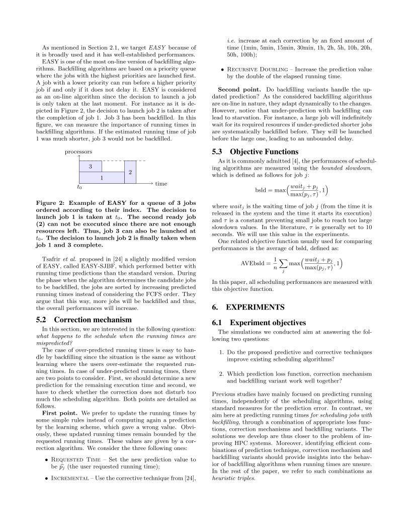
EASY is one of the most on-line version of backfilling algo-rithms. Backfilling algorithms are based on a priority queuewhere the jobs with the highest priorities are launched first.A job with a lower priority can run before a higher priorityjob if and only if it does not delay it. EASY is consideredas an on-line algorithm since the decision to launch a jobis only taken at the last moment. For instance as it is de-picted in Figure 2, the decision to launch job 2 is taken afterthe completion of job 1. Job 3 has been backfilled. In thisfigure, we can measure the importance of running times inbackfilling algorithms. If the estimated running time of job1 was much shorter, job 3 would not be backfilled.
time
processors
t0
12
3
Figure 2: Example of EASY for a queue of 3 jobsordered according to their index. The decision tolaunch job 1 is taken at t0. The second ready job(2) can not be executed since there are not enoughresources left. Thus, job 3 can also be launched att0. The decision to launch job 2 is finally taken whenjob 1 and 3 complete.
Tsafrir et al. proposed in [24] a slightly modified versionof EASY, called EASY-SJBF, which performed better withrunning time predictions than the standard version. Duringthe phase when the algorithm determines the candidate jobsto be backfilled, the jobs are sorted by increasing predictedrunning times instead of considering the FCFS order. Theyargue that this way, more jobs will be backfilled and thus,the overall performances will increase.
5.2 Correction mechanismIn this section, we are interested in the following question:
what happens to the schedule when the running times aremispredicted?
The case of over-predicted running times is easy to han-dle by backfilling since the situation is the same as withoutlearning where the users over-estimate the requested run-ning times. In case of under-predicted running times, thereare two points to consider. First, we should determine a newprediction for the remaining execution time and second, wehave to check whether the correction does not disturb toomuch the scheduling algorithm. Both points are detailed asfollows.
First point. We prefer to update the running times bysome simple rules instead of computing again a predictionby the learning scheme, which gave a wrong value. Obvi-ously, these updated running times remain bounded by therequested running times. These values are given by a cor-rection algorithm. We consider the three following ones:
• Requested Time – Set the new prediction value tobe pj (the user requested running time);
• Incremental – Use the corrective technique from [24],
i.e. increase at each correction by an fixed amount oftime (1min, 5min, 15min, 30min, 1h, 2h, 5h, 10h, 20h,50h, 100h);
• Recursive Doubling – Increase the prediction valueby the double of the elapsed running time.
Second point. Do backfilling variants handle the up-dated prediction? As the considered backfilling algorithmsare on-line in nature, they adapt dynamically to the changes.However, notice that under-prediction with backfilling canlead to starvation. For instance, a large job will indefinitelywait for its required resources if under-predicted shorter jobsare systematically backfilled before. They will be launchedbefore the large one, leading to an unbounded delay.
5.3 Objective FunctionsAs it is commonly admitted [4], the performances of schedul-
ing algorithms are measured using the bounded slowdown,which is defined as follows for job j:
bsld = max(waitj + pj
max(pj , τ), 1)
where waitj is the waiting time of job j (from the time it isreleased in the system and the time it starts its execution)and τ is a constant preventing small jobs to reach too largeslowdown values. In the literature, τ is generally set to 10seconds. We will use this value in the experiments.
One related objective function usually used for comparingperformances is the average of bsld, defined as:
AVEbsld =1
n
∑j
max(waitj + pj
max(pj , τ), 1)
In this paper, all scheduling performances are measured withthis objective function.
6. EXPERIMENTS
6.1 Experiment objectivesThe simulations we conducted aim at answering the fol-
lowing two questions:
1. Do the proposed predictive and corrective techniquesimprove existing scheduling algorithms?
2. Which prediction loss function, correction mechanismand backfilling variant work well together?
Previous studies have mainly focused on predicting runningtimes, independently of the scheduling algorithms, usingstandard measures for the prediction error. In contrast, weaim here at predicting running times for scheduling jobs withbackfilling, through a combination of appropriate loss func-tions, correction mechanisms and backfilling variants. Thesolutions we develop are thus closer to the problem of im-proving HPC systems. Moreover, identifying efficient com-binations of prediction technique, correction mechanism andbackfilling variants should provide insights into the behav-ior of backfilling algorithms when running times are unsure.In the rest of the paper, we refer to such combinations asheuristic triples.
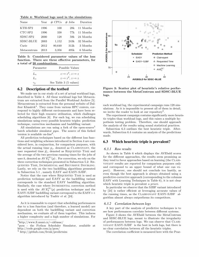
Table 4: Workload logs used in the simulations.
Name Year # CPUs # Jobs Duration
KTH-SP2 1996 100 28k 11 Months
CTC-SP2 1996 338 77k 11 Months
SDSC-SP2 2000 128 59k 24 Months
SDSC-BLUE 2003 1,152 243k 32 Months
Curie 2012 80,640 312k 3 Months
Metacentrum 2013 3,356 495k 6 Months
Table 5: Considered parameter values of the lossfunction. There are three effective parameters, fora total of 20 combinations.
Parameter Possible Values
Lu z 7→ z2, z 7→ z
Lo z 7→ z2, z 7→ z
γj See Table 3 (5 values)
6.2 Description of the testbedWe make use in our study of a set of actual workload logs,
described in Table 4. All these workload logs but Metacen-trum are extracted from the Parallel Workload Archive [5].Metacentrum is extracted from the personal website of Dal-ibor Klusacek4. They come from various HPC centers, cor-respond to highly different environments and have been se-lected for their high resource utilization, which challengesscheduling algorithms [6]. For each log, we run schedulingsimulations using every possible heuristic triples: predictiontechnique, correction mechanism and backfilling variant.
All simulations are run using a fork of the open-source5
batch scheduler simulator pyss. The source of this forkedversion is available on-line6.
All prediction techniques based on the different loss func-tions and weighting schemes introduced in Section 4 are con-sidered here, in conjunction, for comparison purposes, withthe actual running time pj , denoted as Clairvoyant, theuser requested time pj , denoted as Requested Time andthe average of the two previous running times for the jobs of
user k, denoted asAV E(k)2 (p) . For correction, we rely on the
three correction techniques presented in Subsection 5.2: Re-quested Time, Incremental and Recursive Doubling.Lastly, we rely on the two backfilling algorithms presentedin Subsection 5.1 , namely EASY and EASY-SJBF.
Notice that the case where Requested Time is used asprediction technique and EASY as the backfilling variantcorresponds to the standard EASY backfilling algorithm.Similarly, the case where Incremental correction method
is used with the AV E(k)2 (p) prediction technique and the
EASY-SJBF backfilling variant correspond to the EASY++algorithm introduced by Tsafrir et al. [24].
As it is reasonable to expect that scheduling performancesdue to a loss function (and therefore, a learned model) aredependent on both the backfilling variant and correctionmechanism, we evaluate all of them together. This inducesa higher complexity and a high number of simulations. For
4http://www.fi.muni.cz/∼xklusac/5pyss - the Python Scheduler Simulator, available athttp://code.google.com/p/pyss/6 http://github.com/freuk/predictsim
●
●
70
80
90
20 30 40AVGBSLD for SDSC−BLUE
AVG
BS
LD fo
r M
etaC
entr
um
Scheduler
●
●
EASY
EASY−SJBF
Prediction Method
● Clairvoyant
Requested Time
Machine Learning
AVE2(k)
Figure 3: Scatter plot of heuristic’s relative perfor-mance between the MetaCentrum and SDSC-BLUElogs.
each workload log, the experimental campaign runs 128 sim-ulations. As it is impossible to present all of them in detail,we invite the reader to look at our repository6.
The experiment campaign contains significantly more heuris-tic triples than workload logs, and this raises a multiple hy-pothesis testing problem. Therefore, one should approachthe analysis of the results using sound statistical practices.
Subsection 6.3 outlines the best heuristic triple. After-wards, Subsection 6.4 contains an analysis of the predictionsmade.
6.3 Which heuristic triple is prevalent?
6.3.1 Raw resultsAs shown in Table 6 which displays the AVEbsld scores
for the different approaches, the results seem promising asthey tend to favor approaches based on learning (the Clair-voyant results are reported for comparison purposes onlyand correspond to an upper bound of what one can ex-pect). However, one should not conclude too hastily, aseven though the best approach is always obtained using apredictive-corrective approach (corresponding to the columnsEASY with Learning Techniques in Table 6), it is not clearwhich heuristic triple is prevalent a priori.
In particular we observe that the SJBF variant introducedby [24] is rather efficient at leveraging accurate values ofthe running times, as the Clairvoyant EASY-SJBF al-gorithm almost always outperforms its competitors.
6.3.2 Correlation between logsA key part of the analysis of predictive techniques is to
see how performances correlate between different systems.Figure 3 shows the AVEbsld between the MetaCentrum
and SDSC-BLUE logs, meant to illustrate the irregularityof performances between logs. We can observe that Clair-voyant EASY-SJBF is the best in both logs, but there isno clear correlation between all the heuristic triples.
The correlation coefficient is measured here with the Pear-
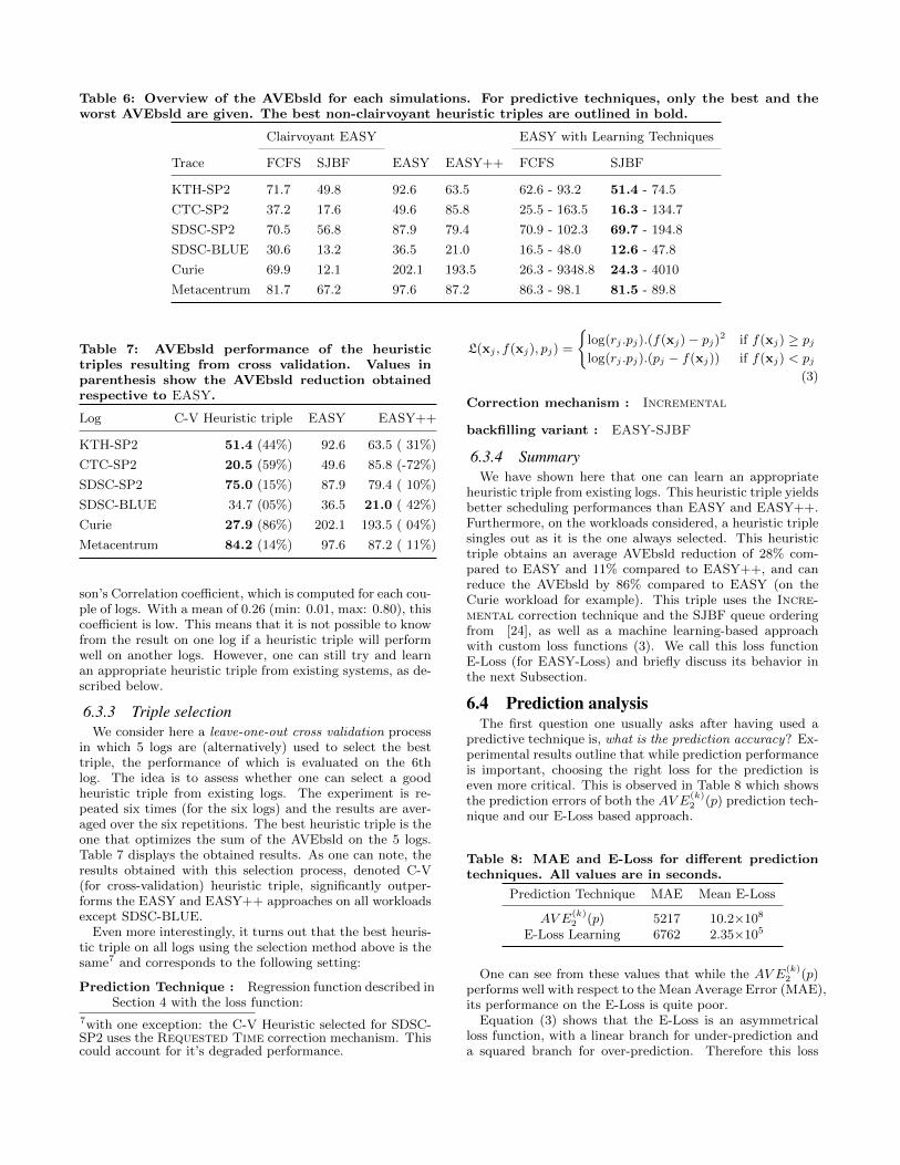
Table 6: Overview of the AVEbsld for each simulations. For predictive techniques, only the best and theworst AVEbsld are given. The best non-clairvoyant heuristic triples are outlined in bold.
Clairvoyant EASY EASY with Learning Techniques
Trace FCFS SJBF EASY EASY++ FCFS SJBF
KTH-SP2 71.7 49.8 92.6 63.5 62.6 - 93.2 51.4 - 74.5
CTC-SP2 37.2 17.6 49.6 85.8 25.5 - 163.5 16.3 - 134.7
SDSC-SP2 70.5 56.8 87.9 79.4 70.9 - 102.3 69.7 - 194.8
SDSC-BLUE 30.6 13.2 36.5 21.0 16.5 - 48.0 12.6 - 47.8
Curie 69.9 12.1 202.1 193.5 26.3 - 9348.8 24.3 - 4010
Metacentrum 81.7 67.2 97.6 87.2 86.3 - 98.1 81.5 - 89.8
Table 7: AVEbsld performance of the heuristictriples resulting from cross validation. Values inparenthesis show the AVEbsld reduction obtainedrespective to EASY.
Log C-V Heuristic triple EASY EASY++
KTH-SP2 51.4 (44%) 92.6 63.5 ( 31%)
CTC-SP2 20.5 (59%) 49.6 85.8 (-72%)
SDSC-SP2 75.0 (15%) 87.9 79.4 ( 10%)
SDSC-BLUE 34.7 (05%) 36.5 21.0 ( 42%)
Curie 27.9 (86%) 202.1 193.5 ( 04%)
Metacentrum 84.2 (14%) 97.6 87.2 ( 11%)
son’s Correlation coefficient, which is computed for each cou-ple of logs. With a mean of 0.26 (min: 0.01, max: 0.80), thiscoefficient is low. This means that it is not possible to knowfrom the result on one log if a heuristic triple will performwell on another logs. However, one can still try and learnan appropriate heuristic triple from existing systems, as de-scribed below.
6.3.3 Triple selectionWe consider here a leave-one-out cross validation process
in which 5 logs are (alternatively) used to select the besttriple, the performance of which is evaluated on the 6thlog. The idea is to assess whether one can select a goodheuristic triple from existing logs. The experiment is re-peated six times (for the six logs) and the results are aver-aged over the six repetitions. The best heuristic triple is theone that optimizes the sum of the AVEbsld on the 5 logs.Table 7 displays the obtained results. As one can note, theresults obtained with this selection process, denoted C-V(for cross-validation) heuristic triple, significantly outper-forms the EASY and EASY++ approaches on all workloadsexcept SDSC-BLUE.
Even more interestingly, it turns out that the best heuris-tic triple on all logs using the selection method above is thesame7 and corresponds to the following setting:
Prediction Technique : Regression function described inSection 4 with the loss function:
7with one exception: the C-V Heuristic selected for SDSC-SP2 uses the Requested Time correction mechanism. Thiscould account for it’s degraded performance.
L(xj , f(xj), pj) =
{log(rj .pj).(f(xj)− pj)2 if f(xj) ≥ pjlog(rj .pj).(pj − f(xj)) if f(xj) < pj
(3)
Correction mechanism : Incremental
backfilling variant : EASY-SJBF
6.3.4 SummaryWe have shown here that one can learn an appropriate
heuristic triple from existing logs. This heuristic triple yieldsbetter scheduling performances than EASY and EASY++.Furthermore, on the workloads considered, a heuristic triplesingles out as it is the one always selected. This heuristictriple obtains an average AVEbsld reduction of 28% com-pared to EASY and 11% compared to EASY++, and canreduce the AVEbsld by 86% compared to EASY (on theCurie workload for example). This triple uses the Incre-mental correction technique and the SJBF queue orderingfrom [24], as well as a machine learning-based approachwith custom loss functions (3). We call this loss functionE-Loss (for EASY-Loss) and briefly discuss its behavior inthe next Subsection.
6.4 Prediction analysisThe first question one usually asks after having used a
predictive technique is, what is the prediction accuracy? Ex-perimental results outline that while prediction performanceis important, choosing the right loss for the prediction iseven more critical. This is observed in Table 8 which showsthe prediction errors of both the AV E
(k)2 (p) prediction tech-
nique and our E-Loss based approach.
Table 8: MAE and E-Loss for different predictiontechniques. All values are in seconds.
Prediction Technique MAE Mean E-Loss
AV E(k)2 (p) 5217 10.2×10⁸
E-Loss Learning 6762 2.35×10⁵
One can see from these values that while the AV E(k)2 (p)
performs well with respect to the Mean Average Error (MAE),its performance on the E-Loss is quite poor.
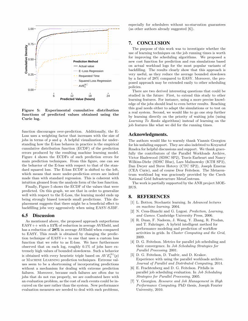
Equation (3) shows that the E-Loss is an asymmetricalloss function, with a linear branch for under-prediction anda squared branch for over-prediction. Therefore this loss
0.00
0.25
0.50
0.75
1.00
6 12 18 24Predicted Value (hours)
Cum
ulat
ive
Den
sity
Prediction Method
Actual value
E−Loss Regression
Requested Time
Squared Loss Regression
AVE2(k)
Figure 5: Experimental cumulative distributionfunctions of predicted values obtained using theCurie log.
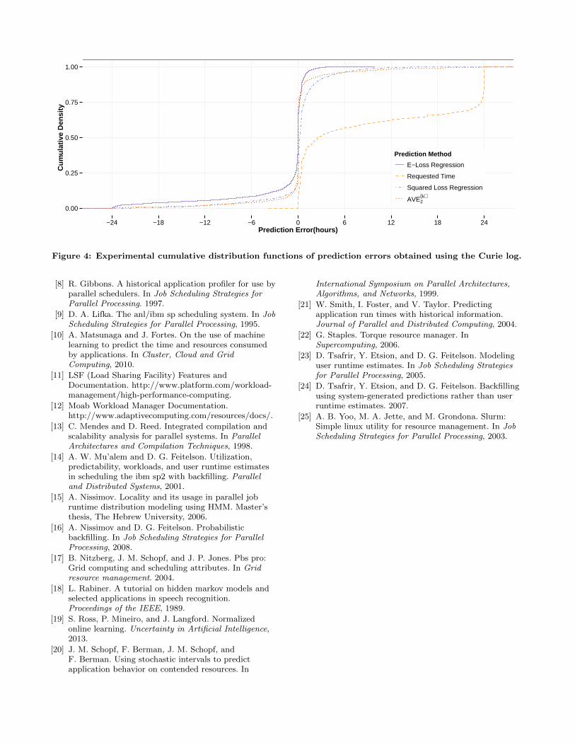
function discourages over-prediction. Additionally, the E-Loss uses a weighting factor that increases with the size ofjobs in terms of p and q. A helpful visualization for under-standing how the E-loss behaves in practice is the empiricalcumulative distribution function (ECDF) of the predictionerrors produced by the resulting machine learning model.Figure 4 shows the ECDFs of such prediction errors formain prediction techniques. From this figure, one can seethe behavior of the E-loss with respect to that of the stan-dard squared loss. The E-loss ECDF is shifted to the left,which means that more under-prediction errors are indeedmade than with standard regression. This is coherent withintuition gleaned from the analysis form of the loss function.
Finally, Figure 5 shows the ECDF of the values that werepredicted. On this graph, we see that in order to generalizewell with respect to the E-Loss, the learning model ends upbeing strongly biased towards small predictions. This dis-placement suggests that there might be a beneficial effect tobackfilling jobs very aggressively when using EASY-SJBF.
6.5 DiscussionAs mentioned above, the proposed approach outperforms
EASY++ with a 11% of reduction in average AVEbsld, andhas a reduction of 28% in average AVEbsld when comparedto EASY. This result is obtained by changing the predic-tion technique of EASY++ to one that uses a custom lossfunction that we refer to as E-loss. We have furthermoreobserved that on each log, roughly 0.1% of jobs have ex-tremely high values of bounded slowdowns. Such a behavior
is obtained with every heuristic triple based on AV E(k)2 (p)
or Machine Learning prediction techniques. Extreme val-ues seem to be a shortcoming of incorporating predictionswithout a mechanism for dealing with extreme predictionfailures. Moreover, because such failures are often due tojobs that do not run properly, we are confronted here withan evaluation problem, as the cost of such events could be in-curred on the user rather than the system. New performanceevaluation measures are needed to deal with such problems,
especially for schedulers without no-starvation guarantees(as other authors already suggested [6]).
7. CONCLUSIONThe purpose of this work was to investigate whether the
use of learning techniques on the job running times is worthfor improving the scheduling algorithms. We proposed anew cost function for prediction and run simulations basedon actual workload logs for the most popular variants ofbackfilling. The results clearly show that this approach isvery useful, as they reduce the average bounded slowdownby a factor of 28% compared to EASY. Moreover, the pro-posed approach may be extended easily to other schedulingpolicies.
There are two derived interesting questions that could bestudied in the future: First, to extend this study to otherlearning features. For instance, using a more precise knowl-edge of the jobs should lead to even better results. Reachingthis goal needs either to adapt the simulations or to test ona real system. Second, we would like to go one step furtherby learning directly on the priority of waiting jobs (usingLearning To Ranks algorithms) instead of learning on thejob features like what we did for the running times.
Acknowledgments.The authors would like to warmly thank Yiannis Georgioufor his unfailing support. They are also indebted to KrzysztofRzadca for helpful discussions and support. We thank grace-fully the contributors of the Parallel Workloads Archive,Victor Hazlewood (SDSC SP2), Travis Earheart and NancyWilkins-Diehr (SDSC Blue), Lars Malinowsky (KTH SP2),Dan Dwyer and Steve Hotovy (CTC SP2), Joseph Emeras(CEA Curie), and of course Dror Feitelson. The Metacen-trum workload log was graciously provided by the CzechNational Grid Infrastructure MetaCentrum.
The work is partially supported by the ANR project MOE-BUS.
8. REFERENCES[1] L. Bottou. Stochastic learning. In Advanced lectures
on machine learning. 2004.
[2] N. Cesa-Bianchi and G. Lugosi. Prediction, Learning,and Games. Cambridge University Press, 2006.
[3] R. Duan, F. Nadeem, J. Wang, Y. Zhang, R. Prodan,and T. Fahringer. A hybrid intelligent method forperformance modeling and prediction of workflowactivities in grids. In Cluster Computing and the Grid,2009.
[4] D. G. Feitelson. Metrics for parallel job scheduling andtheir convergence. In Job Scheduling Strategies forParallel Processing. 2001.
[5] D. G. Feitelson, D. Tsafrir, and D. Krakov.Experience with using the parallel workloads archive.Journal of Parallel and Distributed Computing, 2014.
[6] E. Frachtenberg and D. G. Feitelson. Pitfalls inparallel job scheduling evaluation. In Job SchedulingStrategies for Parallel Processing, 2005.
[7] Y. Georgiou. Resource and Job Management in HighPerformance Computing. PhD thesis, Joseph FourierUniversity, 2010.
0.00
0.25
0.50
0.75
1.00
−6−12−18−24 0 6 12 18 24Prediction Error(hours)
Cum
ulat
ive
Den
sity
Prediction Method
E−Loss Regression
Requested Time
Squared Loss Regression
AVE2(k)
Figure 4: Experimental cumulative distribution functions of prediction errors obtained using the Curie log.
[8] R. Gibbons. A historical application profiler for use byparallel schedulers. In Job Scheduling Strategies forParallel Processing. 1997.
[9] D. A. Lifka. The anl/ibm sp scheduling system. In JobScheduling Strategies for Parallel Processing, 1995.
[10] A. Matsunaga and J. Fortes. On the use of machinelearning to predict the time and resources consumedby applications. In Cluster, Cloud and GridComputing, 2010.
[11] LSF (Load Sharing Facility) Features andDocumentation. http://www.platform.com/workload-management/high-performance-computing.
[12] Moab Workload Manager Documentation.http://www.adaptivecomputing.com/resources/docs/.
[13] C. Mendes and D. Reed. Integrated compilation andscalability analysis for parallel systems. In ParallelArchitectures and Compilation Techniques, 1998.
[14] A. W. Mu’alem and D. G. Feitelson. Utilization,predictability, workloads, and user runtime estimatesin scheduling the ibm sp2 with backfilling. Paralleland Distributed Systems, 2001.
[15] A. Nissimov. Locality and its usage in parallel jobruntime distribution modeling using HMM. Master’sthesis, The Hebrew University, 2006.
[16] A. Nissimov and D. G. Feitelson. Probabilisticbackfilling. In Job Scheduling Strategies for ParallelProcessing, 2008.
[17] B. Nitzberg, J. M. Schopf, and J. P. Jones. Pbs pro:Grid computing and scheduling attributes. In Gridresource management. 2004.
[18] L. Rabiner. A tutorial on hidden markov models andselected applications in speech recognition.Proceedings of the IEEE, 1989.
[19] S. Ross, P. Mineiro, and J. Langford. Normalizedonline learning. Uncertainty in Artificial Intelligence,2013.
[20] J. M. Schopf, F. Berman, J. M. Schopf, andF. Berman. Using stochastic intervals to predictapplication behavior on contended resources. In
International Symposium on Parallel Architectures,Algorithms, and Networks, 1999.
[21] W. Smith, I. Foster, and V. Taylor. Predictingapplication run times with historical information.Journal of Parallel and Distributed Computing, 2004.
[22] G. Staples. Torque resource manager. InSupercomputing, 2006.
[23] D. Tsafrir, Y. Etsion, and D. G. Feitelson. Modelinguser runtime estimates. In Job Scheduling Strategiesfor Parallel Processing, 2005.
[24] D. Tsafrir, Y. Etsion, and D. G. Feitelson. Backfillingusing system-generated predictions rather than userruntime estimates. 2007.
[25] A. B. Yoo, M. A. Jette, and M. Grondona. Slurm:Simple linux utility for resource management. In JobScheduling Strategies for Parallel Processing, 2003.