an integrated approach to parallel scheduling using gang-scheduling, backfilling, and migration

An Integrated Approach to Parallel Scheduling UsingGang-Scheduling, Backfilling and Migration

Y. Zhangy H. Frankez J. E. Moreiraz A. Sivasubramaniamy

y Department of Computer Science& Engineering z IBM T. J. Watson Research CenterThe Pennsylvania State University P. O. Box 218

University Park PA 16802 Yorktown Heights NY 10598-0218fyyzhang, [email protected] ffrankeh, [email protected]

Abstract

Effective scheduling strategies to improve response times,throughput, and utilization are an important considerationin large supercomputing environments. Such machineshave traditionally used space-sharing strategies to accom-modate multiple jobs at the same time. This approach,however, can result in low system utilization and largejob wait times. This paper discusses three techniques thatcan be used beyond simple space-sharing to greatly im-prove the performance figures of large parallel systems.The first technique we analyze is backfilling, the secondis gang-scheduling, and the third is migration. The maincontribution of this paper is an evaluation of the benefitsfrom combining the above techniques. We demonstratethat, under certain conditions, a strategy that combinesbackfilling, gang-scheduling, and migration is always bet-ter than the individual strategies for all quality of serviceparameters that we consider.

1 Introduction

Large scale parallel machines are essential to meet theneeds of demanding applications at supercomputing en-vironments. In that context, it is imperative to provideeffective scheduling strategies to meet the desired qual-ity of service parameters from both user and system per-spectives. Specifically, we would like to reduce responseand wait times for a job, minimize the slowdown that ajob experiences in a multiprogrammed setting comparedto when it is run in isolation, maximize the throughput andutilization of the system, and be fair to all jobs regardlessof their size or execution times.

Scheduling strategies can have a significant impact onthe performance characteristics of a large parallel sys-tem [2, 3, 4, 7, 10, 13, 14, 17, 18, 21, 22]. Early strategiesused a space-sharing approach, wherein jobs can run con-currently on different nodes of the machine at the same

time, but each node is exclusively assigned to a job. Sub-mitted jobs are kept in a priority queue which is alwaystraversed according to a priority policy in search of thenext job to execute. Space sharing in isolation can re-sult in poor utilization since there could be nodes that areunutilized despite a waiting queue of jobs. Furthermore,the wait and response times for jobs with an exclusivelyspace-sharing strategy can be relatively high.

We analyze three approaches to alleviate the problemswith space sharing scheduling. The first is a techniquecalled backfilling [6, 14], which attempts to assign unuti-lized nodes to jobs that are behind in the priority queue (ofwaiting jobs), rather than keep them idle. To prevent star-vation for larger jobs, (conservative) backfilling requiresthat a job selected out of order completes before the jobsthat are ahead of it in the priority queue are scheduled tostart. This approach requires the users to provide an esti-mate of job execution times, in addition to the number ofnodes required by each job. Jobs that exceed their execu-tion time are killed. This encourages users to overestimatethe execution time of their jobs.

The second approach is to add a time-sharing dimen-sion to space sharing using a technique called gang-scheduling or coscheduling [16, 22]. This technique vir-tualizes the physical machine by slicing the time axisinto multiple virtual machines. Tasks of a parallel jobare coscheduled to run in the same time-slices (same vir-tual machines). In some cases it may be advantageous toschedule the same job to run on multiple virtual machines(multiple time-slices). The number of virtual machinescreated (equal to the number of time slices), is called themultiprogramming level (MPL) of the system. This multi-programming level in general depends on how many jobscan be executed concurrently, but is typically limited bysystem resources. This approach opens more opportuni-ties for the execution of parallel jobs, and is thus quite ef-fective in reducing the wait time, at the expense of increas-ing the apparent job execution time. Gang-scheduling

does not depend on estimates for job execution time.

The third approach is to dynamically migrate tasks ofa parallel job. Migration delivers flexibility of adjustingyour schedule to avoid fragmentation [3, 4]. Migrationis particularly important when collocation in space and/ortime of tasks is necessary. Collocation in space is im-portant in some architectures to guarantee proper commu-nication among tasks (e.g., Cray T3D, CM-5, and BlueGene). Collocation in time is important when tasks haveto be running concurrently to make progress in communi-cation (e.g., gang-scheduling).

It is a logical next step to attempt to combine these ap-proaches – gang-scheduling, backfilling, and migration– to deliver even better performance for large parallelsystems. Progressing to combined approaches requiresa careful examination of several issues related to back-filling, gang-scheduling, and migration. Using detailedsimulations based on stochastic models derived from realworkloads, this paper analyzes (i) the impact of over-estimating job execution times on the effectiveness ofbackfilling, (ii) a strategy for combining gang-schedulingand backfilling, (iii) the impact of migration in a gang-scheduled system, and (iv) the impact of combining gang-scheduling, migration, and backfilling in one schedulingsystem.

We find that overestimating job execution times doesnot really impact the quality of service parameters, re-gardless of the degree of overestimation. As a result, wecan conservatively estimate the execution time of a job ina coscheduled system to be the multiprogramming level(MPL) times the estimated job execution time in a ded-icated setting after considering the associated overheads,such as context-switch overhead. These results help usconstruct a backfilling gang-scheduling system, calledBGS, which fills in holes in the Ousterhout schedulingmatrix [16] with jobs that are not necessarily in first-comefirst-serve (FCFS) order. It is clearly demonstrated that,under certain conditions, this combined strategy is alwaysbetter than the individual gang-scheduling or backfillingstrategies for all the quality of service parameters that weconsider. By combining gang-scheduling and migrationwe can further improve the system performance param-eters. The improvement is larger when applied to plaingang-scheduling (without backfilling), although the ab-solute best performance was achieved by combining allthree techniques: gang-scheduling, backfilling, and mi-gration.

The rest of this paper is organized as follows. Sec-tion 2 describes our approach to modeling parallel jobworkloads and obtaining performance characteristics ofscheduling systems. It also characterizes our base work-load quantitatively. Section 3 analyzes the impact ofjob execution time estimation on the overall performance

from system and user perspectives. We show that rele-vant performance parameters are almost invariant to theaccuracy of average job execution time estimation. Sec-tion 4 describes gang-scheduling, and the various phasesinvolved in computing a time-sharing schedule. Sec-tion 5 demonstrates the significant improvements in per-formance that can be achieved with time-sharing tech-niques, particularly when enhanced with backfilling andmigration. Finally, Section 6 presents our conclusions andpossible directions for future work.

2 Evaluation methodology

When selecting and developing job schedulers for use inlarge parallel system installations, it is important to un-derstand their expected performance. The first stage is tohave a characterization of the workload and a procedureto synthetically generate the expected workloads. Ourmethodology for generating these workloads, and fromthere obtaining performance parameters, involves the fol-lowing steps:

1. Fit a typical workload with mathematical models.

2. Generate synthetic workloads based on the derivedmathematical models.

3. Simulate the behavior of the different schedulingpolicies for those workloads.

4. Determine the parameters of interest for the differentscheduling policies.

We now describe these steps in more detail.

2.1 Workload modeling

Parallel workloads often are over-dispersive. That is, bothjob interarrival time distribution and job service time (ex-ecution time on a dedicated system) distribution have co-efficients of variation that are greater than one. Distribu-tions with coefficient of variation greater than one are alsoreferred to as long-tailed distributions, and can be fittedadequately with Hyper Erlang Distributions of CommonOrder. In [12] such a model was developed, and its ef-ficacy demonstrated by using it to fit a typical workloadfrom the Cornell University Theory Center. Here we usethis model to fit a typical workload from the ASCI Blue-Pacific System at Lawrence Livermore National Labora-tory (LLNL), an IBM RS/6000 SP.

Our modeling procedure involves the following steps:

1. First we group the jobs into classes, based on thenumber of nodes they require for execution. Eachclass is a bin in which the upper boundary is a powerof 2.

2. Then we model the interarrival time distribution foreach class, and the service time distribution for eachclass as follows:

(a) From the job traces, we compute the first threemoments of the observed interarrival time andthe first three moments of the observed servicetime.

(b) Then we select the Hyper Erlang Distributionof Common Order that fits these 3 observedmoments. We choose to fit the moments of themodel against those of the actual data becausethe first 3 moments usually capture the genericfeatures of the workload. These three momentscarry the information on the mean, variance,and skewness of the random variable, respec-tively.

Next, we generate various synthetic workloads from theobserved workload by varying the interarrival rate and ser-vice time used. The Hyper Erlang parameters for thesesynthetic workloads are obtained by multiplying the inter-arrival rate and the service time each by a separate mul-tiplicative factor, and by specifying the number of jobsto generate. From these model parameters synthetic jobtraces are obtained using the procedure described in [12].Finally, we simulate the effects of these synthetic work-loads and observe the results.

Within a workload trace, each job is described by itsarrival time, the number of nodes it uses, its executiontime on a dedicated system, and an overestimation factor.Backfilling strategies require an estimate of the job exe-cution time. In a typical system, it is up to each user toprovide these estimates. This estimated execution time isalways greater than or equal to the actual execution time,since jobs are terminated after reaching this limit. We cap-ture this discrepancy between estimated and actual exe-cution times for parallel jobs through anoverestimationfactor. The overestimation factor for each job is the ratiobetween its estimated and actual execution times. Dur-ing simulation, the estimated execution time is used ex-clusively for performing job scheduling, while the actualexecution time is used to define the job finish event.

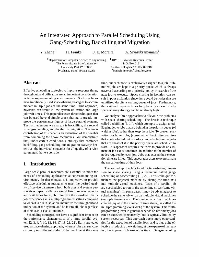
In this paper, we adopt what we call the� model ofoverestimation. In the� model,� is the fraction of jobsthat terminate at exactly the estimated time. This typicallycorresponds to jobs that are killed by the system becausethey reach the limit of their allocated time. The rest of thejobs (1 � �) are distributed such that the distribution ofjobs that end at a certain fraction of their estimated timeis uniform. This distribution is shown in Figure 1. It hasbeen shown to represent well actual job behavior in largesystems [6]. To obtain the desired distribution for execu-tion times in the� model, in our simulations we compute

the overestimation factor as follows: Lety be a uniformlydistributed random number in the range0 � y < 1. Ify < �, then the overestimation factor is 1 (i.e., estimatedtime = execution time). Ify � �, then the overestimationfactor is(1��)=(1� y).

0 0.1 0.2 0.3 0.4 0.5 0.6 0.7 0.8 0.9 1

1−Φ

Φ

Execution time as fraction of estimated time

Pro

babi

lity

dens

ity fu

nctio

n p(

x) fo

r jo

bs

Distribution of job execution time

Figure 1: The� models for overestimation.

2.2 Workload characteristics

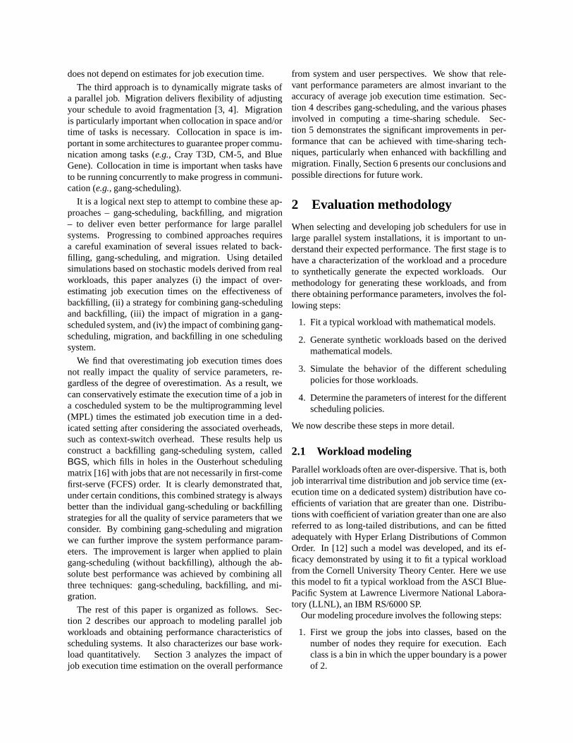
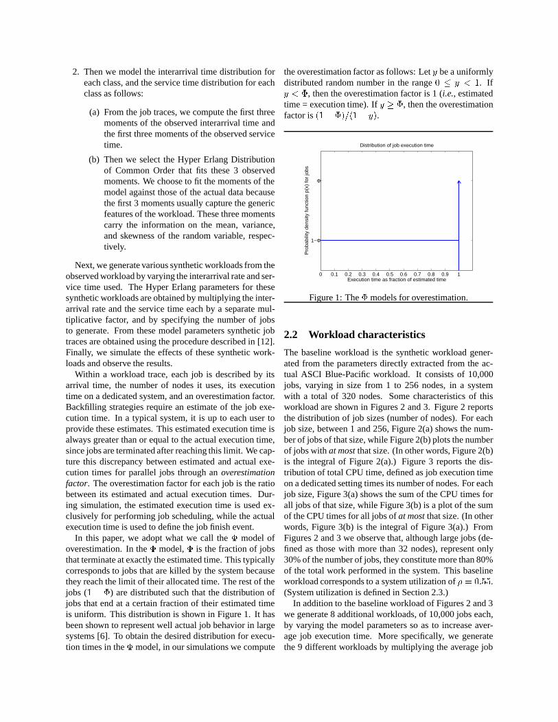
The baseline workload is the synthetic workload gener-ated from the parameters directly extracted from the ac-tual ASCI Blue-Pacific workload. It consists of 10,000jobs, varying in size from 1 to 256 nodes, in a systemwith a total of 320 nodes. Some characteristics of thisworkload are shown in Figures 2 and 3. Figure 2 reportsthe distribution of job sizes (number of nodes). For eachjob size, between 1 and 256, Figure 2(a) shows the num-ber of jobs of that size, while Figure 2(b) plots the numberof jobs withat mostthat size. (In other words, Figure 2(b)is the integral of Figure 2(a).) Figure 3 reports the dis-tribution of total CPU time, defined as job execution timeon a dedicated setting times its number of nodes. For eachjob size, Figure 3(a) shows the sum of the CPU times forall jobs of that size, while Figure 3(b) is a plot of the sumof the CPU times for all jobs ofat mostthat size. (In otherwords, Figure 3(b) is the integral of Figure 3(a).) FromFigures 2 and 3 we observe that, although large jobs (de-fined as those with more than 32 nodes), represent only30% of the number of jobs, they constitute more than 80%of the total work performed in the system. This baselineworkload corresponds to a system utilization of� = 0:55.(System utilization is defined in Section 2.3.)

In addition to the baseline workload of Figures 2 and 3we generate 8 additional workloads, of 10,000 jobs each,by varying the model parameters so as to increase aver-age job execution time. More specifically, we generatethe 9 different workloads by multiplying the average job

0 32 64 96 128 160 192 224 2560

50

100

150

200

250

300

350

400

450

500

Job size (number of nodes)

Num

ber

of jo

bs

Distribution of job sizes

0 32 64 96 128 160 192 224 2560

1000

2000

3000

4000

5000

6000

7000

8000

9000

10000


Num

ber

of jo

bs

Cumulative distribution of job sizes

(a) (b)

Figure 2: Workload characteristics: distribution of job sizes.

0 32 64 96 128 160 192 224 2560

0.2

0.4

0.6

0.8

1

1.2

1.4

1.6

1.8

2x 10

7


Tot

al C

PU

tim

e (s

)

Distribution of CPU time

0 32 64 96 128 160 192 224 2560

1

2

3

4

5

6

7

8

9

10x 10

8


Tot

al C

PU

tim

e (s

)

Cumulative distribution of CPU time

(a) (b)

Figure 3: Workload characteristics: distribution of cpu time.

execution time by a factor from1:0 to 1:8 in steps of0:1.For a fixed interarrival time, increasing job execution timetypically increases utilization, until the system saturates.

2.3 Performance metrics

The synthetic workloads generated as described in Sec-tion 2.1 are used as input to our event-driven simulator ofvarious scheduling strategies. We simulate a system with320 nodes, and we monitor the following parameters:

� tai : arrival time for jobi.

� tsi : start time for jobi.

� tei : execution time for jobi (in a dedicated setting).

� tfi : finish time for jobi.

� ni: number of nodes used by jobi.

From these we compute:

� tri = tfi � tai : response time for jobi.

� twi = tsi � tai : wait time for jobi.

� si =max(tr

i;�)

max(tei;�) : the slowdown for jobi. To reduce

the statistical impact of very short jobs, it is commonpractice [5, 6] to adopt a minimum execution time of� seconds. This is the reason for themax(�;�) termsin the definition of slowdown. According to [6], weadopt� = 10 seconds.

To report quality of service figures from a user’s perspec-tive we use the average job slowdown and average jobwait time. Job slowdown measures how much slowerthan a dedicated machine the system appears to the users,which is relevant to both interactive and batch jobs. Job

wait time measures how long a job takes to start execu-tion and therefore it is an important measure for inter-active jobs. In addition to objective measures of qualityof service, we also use these averages to characterize thefairness of a scheduling strategy. We evaluate fairness bycomparing average and standard deviation of slowdownand wait time for small jobs, large jobs, and all jobs com-bined. As discussed in Section 2.2, large jobs are thosethat use more than 32 nodes, while small jobs use 32 orfewer nodes.

We measure quality of service from the system’s per-spective with two parameters: utilization and capacityloss. Utilization is the fraction of total system resourcesthat are actually used during the execution of a workload.Let the system haveN nodes and executem jobs, wherejobm is the last job to finish execution. Also, let the firstjob arrive at timet = 0. Utilization is then defined as

� =

Pmi=1 nit

ei

tfm �N(1)

A system incurs loss of capacity when (i) it has jobswaiting in the queue to execute, and (ii) it has empty nodes(either physical or virtual) but, because of fragmentation,it still cannot execute those waiting jobs. Before we candefine loss of capacity, we need to introduce some moreconcepts. Ascheduling eventtakes place whenever a newjob arrives or an executing job terminates. By definition,there are2m scheduling events, occurring at times i, fori = 1; : : : ; 2m. Let ei be the number of nodes left emptybetween scheduling eventsi andi+1. Finally, let�i be 1if there are any jobs waiting in the queue after schedulingeventi, and 0 otherwise. Loss of capacity in a purelyspace-shared system is then defined as

� =

P2m�1i=1 ei( i+1 � i)�i

tfm �N(2)

To compute the loss of capacity in a gang-schedulingsystem, we have to keep track of what happens in eachtime-slice. Please note that here one time-slice is not ex-actly equal to one row in the matrix since the last time-slice could be shorter than a row in time due to the factthat a scheduling event could happen in the middle of arow. Letsi be the number of time slices between schedul-ing eventi and scheduling eventi+1. We can then define

� =

P2m�1i=1 [ei( i+1 � i) + T � CS � si � ni] �i

tfm �N(3)

where

� T is the duration of one row in the matrix;

� CS is the context-switch overhead (as a fraction ofT );

� ni is the number of occupied nodes between schedul-ing eventsi andi+1, more specifically,ni+ei = N .

A system is in a saturated state when increasing the loaddoes not result in an increase in utilization. At this point,the loss of capacity is equal to one minus the maximumachievable utilization. More specifically,� = 1� �max.

3 The impact of overestimation onbackfilling

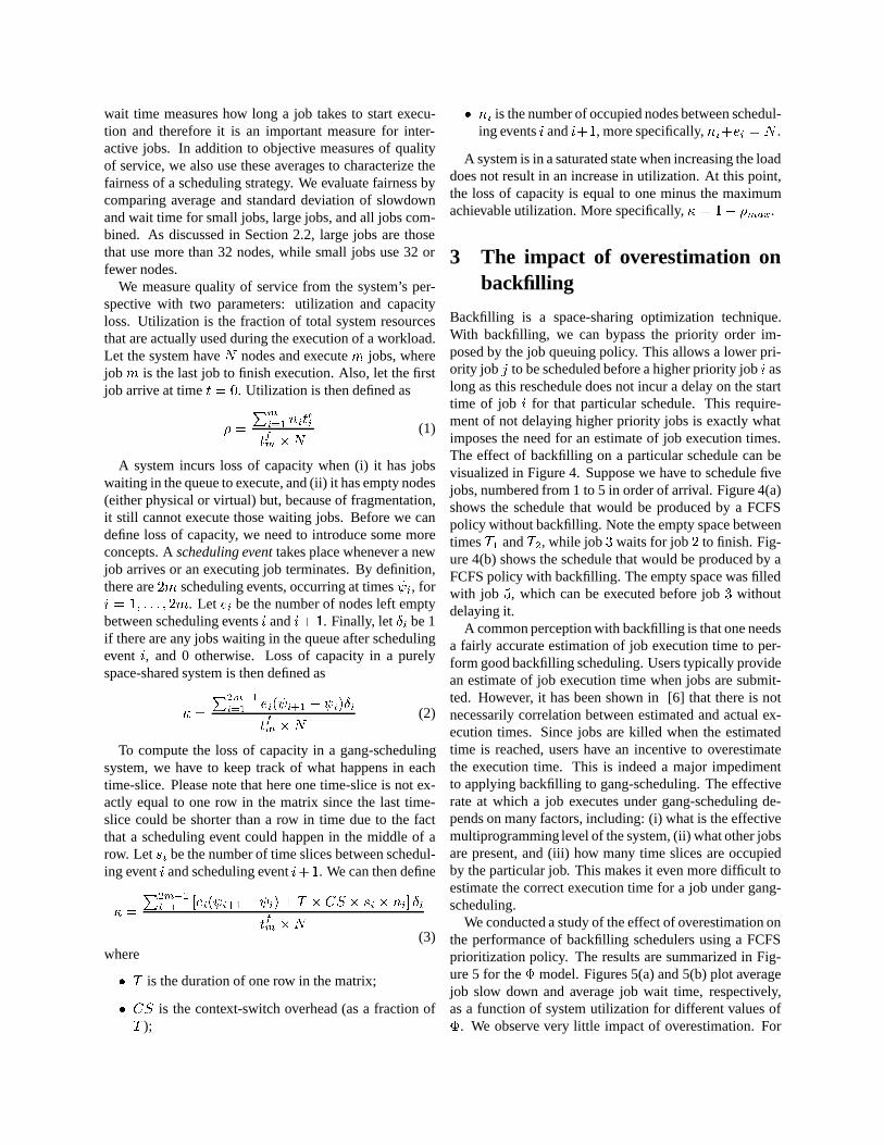
Backfilling is a space-sharing optimization technique.With backfilling, we can bypass the priority order im-posed by the job queuing policy. This allows a lower pri-ority job j to be scheduled before a higher priority jobi aslong as this reschedule does not incur a delay on the starttime of job i for that particular schedule. This require-ment of not delaying higher priority jobs is exactly whatimposes the need for an estimate of job execution times.The effect of backfilling on a particular schedule can bevisualized in Figure 4. Suppose we have to schedule fivejobs, numbered from 1 to 5 in order of arrival. Figure 4(a)shows the schedule that would be produced by a FCFSpolicy without backfilling. Note the empty space betweentimesT1 andT2, while job3 waits for job2 to finish. Fig-ure 4(b) shows the schedule that would be produced by aFCFS policy with backfilling. The empty space was filledwith job 5, which can be executed before job3 withoutdelaying it.

A common perception with backfilling is that one needsa fairly accurate estimation of job execution time to per-form good backfilling scheduling. Users typically providean estimate of job execution time when jobs are submit-ted. However, it has been shown in [6] that there is notnecessarily correlation between estimated and actual ex-ecution times. Since jobs are killed when the estimatedtime is reached, users have an incentive to overestimatethe execution time. This is indeed a major impedimentto applying backfilling to gang-scheduling. The effectiverate at which a job executes under gang-scheduling de-pends on many factors, including: (i) what is the effectivemultiprogramming level of the system, (ii) what other jobsare present, and (iii) how many time slices are occupiedby the particular job. This makes it even more difficult toestimate the correct execution time for a job under gang-scheduling.

We conducted a study of the effect of overestimation onthe performance of backfilling schedulers using a FCFSprioritization policy. The results are summarized in Fig-ure 5 for the� model. Figures 5(a) and 5(b) plot averagejob slow down and average job wait time, respectively,as a function of system utilization for different values of�. We observe very little impact of overestimation. For

time

space

-

6

1

2

3

4

5

T1 T2 time

space

-

6

1

2

3

45

T1 T2(a) (b)

Figure 4: FCFS policy without (a) and with (b) backfilling. Job numbers correspond to their position in the priorityqueue.

utilization up to� = 0:90, overestimation actually helpsin reducing job slowdown. However, we can see a littlebenefit in wait time from more accurate estimates.

We can explain why backfilling is not that sensitive tothe estimated execution time by the following reasoning:On average, overestimation impacts both the jobs that arerunning and the jobs that are waiting. The scheduler com-putes a later finish time for the running jobs, creatinglarger holes in the schedule. The larger holes can thenbe used to accommodate waiting jobs that have overesti-mated execution times. The probability of finding a back-filling candidate effectively does not change with the over-estimation.

Even though the average job behavior is insensitiveto the average degree of overestimation, individual jobscan be affected. To verify that, we group the jobs into10 classes based on how close is their estimated time totheir actual execution time. For the� model, classi,i = 0; : : : ; 9 includes all those jobs for which their ra-tio of execution time to estimated time falls in the range(i � 10%,(i + 1) � 10%]. Figure 6 shows the averagejob wait time for (i) all jobs, (ii) jobs in class 0 (worst es-timators) and (iii) jobs in class 9 (best estimators) when� = 0:2. We observe that those users that provide goodestimates are rewarded with a lower average wait time.The conclusion is that the “quality” of an estimation isnot really defined by how close it is to the actual execu-tion time, but by how much better it is compared to theaverage estimation. Users do get a benefit, and thereforean encouragement, from providing good estimates.

Our findings are in agreement with the work describedin [19]. In that paper, the authors describe mechanismsto more accurately predict job execution times, based onhistorical data. They find that more accurate estimates ofjob execution time lead to more accurate estimates of waittime. The authors do observe an improvement in averagejob wait time, for a particular Argonne National Labora-tory workload, when using their predictors instead of pre-viously published work [1, 9].

4 Gang-scheduling

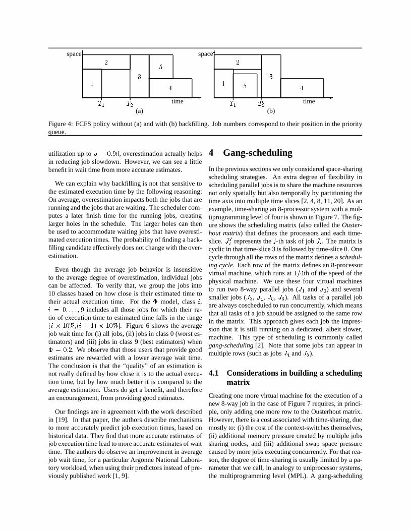
In the previous sections we only considered space-sharingscheduling strategies. An extra degree of flexibility inscheduling parallel jobs is to share the machine resourcesnot only spatially but also temporally by partitioning thetime axis into multiple time slices [2, 4, 8, 11, 20]. As anexample, time-sharing an 8-processor system with a mul-tiprogramming level of four is shown in Figure 7. The fig-ure shows the scheduling matrix (also called theOuster-hout matrix) that defines the processors and each time-slice. Jji represents thej-th task of jobJi. The matrix iscyclic in that time-slice 3 is followed by time-slice 0. Onecycle through all the rows of the matrix defines aschedul-ing cycle.Each row of the matrix defines an 8-processorvirtual machine, which runs at1=4th of the speed of thephysical machine. We use these four virtual machinesto run two 8-way parallel jobs (J1 andJ2) and severalsmaller jobs (J3, J4, J5, J6). All tasks of a parallel jobare always coscheduled to run concurrently, which meansthat all tasks of a job should be assigned to the same rowin the matrix. This approach gives each job the impres-sion that it is still running on a dedicated, albeit slower,machine. This type of scheduling is commonly calledgang-scheduling[2]. Note that some jobs can appear inmultiple rows (such as jobsJ4 andJ5).

4.1 Considerations in building a schedulingmatrix

Creating one more virtual machine for the execution of anew 8-way job in the case of Figure 7 requires, in princi-ple, only adding one more row to the Ousterhout matrix.However, there is a cost associated with time-sharing, duemostly to: (i) the cost of the context-switches themselves,(ii) additional memory pressure created by multiple jobssharing nodes, and (iii) additional swap space pressurecaused by more jobs executing concurrently. For that rea-son, the degree of time-sharing is usually limited by a pa-rameter that we call, in analogy to uniprocessor systems,the multiprogramming level (MPL). A gang-scheduling

0.55 0.6 0.65 0.7 0.75 0.8 0.85 0.9 0.95 10

5

10

15

20

25

30

utilization

Ave

rage

job

wai

t tim

e (X

100

0 se

cond

s)

φ=0.2

φ=0.4

φ=0.6

φ=0.8

φ=1.0

0.55 0.6 0.65 0.7 0.75 0.8 0.85 0.9 0.95 10

10

20

30

40

50

60

70

80

90

100

utilization

Ave

rage

job

slow

dow

n

φ=0.2

φ=0.4

φ=0.6

φ=0.8

φ=1.0

(a) Wait time (b) Slow down

Figure 5: Average job slowdown and wait time for backfilling under� model of overestimation.

0.5 0.55 0.6 0.65 0.7 0.75 0.8 0.85 0.9 0.95 10

5

10

15

20

25

30

utilization

Ave

rage

job

wai

t tim

e (x

1000

sec

onds

)

worst estimators

average

best estimators

Figure 6: The impact of good estimation from a user perspective for the� model of overestimation.

system with multiprogramming level of 1 reverts back toa space-sharing system.

In our particular simulation of gang-scheduling, wemake the following assumptions and scheduling strate-gies:

1. Multiprogramming levels are kept at modest levels,in order to guarantee that the images of all tasks ina node remain in core. This eliminates paging andsignificantly reduces the cost of context switching.Furthermore, the time slices are sized so that the costof the resulting context switches are small. Morespecifically, in our simulations, we use MPL� 5,and CS (context switch overhead fraction)� 5%.

2. Assignments of tasks to processors are static. Thatis, once spatial scheduling is performed for the tasksof a parallel job, they cannot migrate to other nodes.

3. When building the scheduling matrix, we first at-

tempt to schedule as many jobs for execution as pos-sible, constrained by the physical number of proces-sors and the multiprogramming level. Only after thatwe attempt toexpanda job, by making it occupymultiple rows of the matrix. (See jobsJ4 andJ5 inFigure 7.)

4. For a particular instance of the Ousterhout matrix,each job has an assignedhome row. Even if a jobappears in multiple rows, one and only one of themis the home row. The home row of a job can changeduring its life time, when the matrix is recomputed.The purpose of the home row is described in Sec-tion 4.2.

Gang-scheduling is a time-sharing technique that canbe applied together with any prioritization policy. In par-ticular, we have shown in previous work [7, 15] that gang-scheduling is very effective in improving the performanceof FCFS policies. This is in agreement with the results

P0 P1 P2 P3 P4 P5 P6 P7time-slice 0 J1 J1 J1 J1 J1 J1 J1 J1time-slice 1 J2 J2 J2 J2 J2 J2 J2 J2time-slice 2 J3 J3 J3 J3 J4 J4 J5 J5time-slice 3 J6 J6 J6 J6 J4 J4 J5 J5

Figure 7: The scheduling matrix defines spatial and time allocation.

in [4, 17]. We have also shown that gang-schedulingis particularly effective in improving system responsive-ness, as measured by average job wait time. However,gang scheduling alone is not as effective as backfillingin improving average job response time, unless very highmultiprogramming levels are allowed. These may not beachievable in practice by the reasons mentioned in the pre-vious paragraphs.

4.2 The phases of scheduling

Every job arrival or departure constitutes aschedulingeventin the system. For each scheduling event, a newscheduling matrix is computed for the system. Eventhough we analyze various scheduling strategies in thispaper, they all follow an overall organization for comput-ing that matrix, which can be divided into the followingsteps:

1. CleanMatrix: The first phase of a scheduler re-moves every instance of a job in the Ousterhout ma-trix that is not at its assigned home row. Removingduplicates across rows effectively opens the opportu-nity of selecting other waiting jobs for execution.

2. CompactMatrix: This phase moves jobs from lesspopulated rows to more populated rows. It furtherincreases the availability of free slots within a singlerow to maximize the chances of scheduling a largejob.

3. Schedule:This phase attempts to schedule new jobs.We traverse the queue of waiting jobs as dictated bythe given priority policy until no further jobs can befitted into the scheduling matrix.

4. FillMatrix: This phase tries to fill existing holes inthe matrix by replicating jobs from their home rowsinto a set of replicated rows. This operation is essen-tially the opposite ofCleanMatrix .

The exact procedure for each step is dependent on theparticular scheduling strategy and the details will be pre-sented as we discuss each strategy.

5 Scheduling strategies

When analyzing the performance of the time-sharedstrategies we have to take into account the context-switchoverhead. Context switch overhead is the time used by thesystem in suspending a currently running job and resum-ing the next job. During this time, the system is not doinguseful work from a user perspective, and that is why wecharacterize it as overhead. In the IBM RS/6000 SP, con-text switch overhead includes the protocol for detachingand attaching to the communication device. It also in-cludes the operations to stop and continue user processes.When the working set of time-sharing jobs is larger thanthe physical memory of the machine, context switch over-head should also include the time to page in the workingset of the resuming job. For our analysis, we character-ize context switch overhead as a percentage of time slice.Typically, context switch overhead values should be be-tween 0 to 5% of time slice.

5.1 Gang-scheduling (GS)

The first scheduling strategy we analyze is plain gang-scheduling (GS). This strategy is described in Section 4.For gang-scheduling, we implement the four schedulingsteps of Section 4.2 as follows.

CleanMatrix: The implementation of CleanMatrix isbest illustrated with the following algorithm:for i = first row to last row

for all jobs in row iif row i is not home of job, remove job

It eliminates all occurrences of a job in the schedulingmatrix other than the one in its home row.

CompactMatrix: We implement the CompactMatrixstep in gang-scheduling according to the following algo-rithm:for i = least populated row to most populated row

for j = most populated row to i+1for each job in row i

if it can be moved to row j, then move job

We traverse the scheduling matrix from the least popu-lated row to the most populated row. We attempt to findnew homes for the jobs in each row. The goal is to packthe most jobs in the least number of rows.

Schedule: The Schedule phase for gang-scheduling tra-verses the waiting queue in FCFS order. For each job, itlooks for the row with the least number of free columnsin the scheduling matrix that has enough free columns tohold the job. This corresponds to a best fit algorithm. Therow to which the job is assigned becomes its home row.We stop when the next job in the queue cannot be sched-uled right away.

FillMatrix: After the schedule phase completes, weproceed to fill the holes in the matrix with the existingjobs. We use the following algorithm in executing the Fill-Matrix phase.

do{for each job in starting time order

for each row in matrix,if job can be replicated in same columns

do it and break} while matrix changes

The algorithm attempts to replicate each job at leastonce (In the algorithm, once a chance of replicating a jobis found, we stop looking for more chances of replicat-ing the same job, but instead, we start other jobs) , al-though some jobs can be replicated multiple times. We gothrough the jobs in starting time order, but other orderingpolicies can be applied.

5.2 Backfilling gang-scheduling (BGS)

Gang-scheduling and backfilling are two optimizationtechniques that operate on orthogonal axes, space forbackfilling and time for gang scheduling. It is temptingto combine both techniques in one scheduling system thatwe call backfilling gang-scheduling(BGS). In principlethis can be done by treating each of the virtual machinescreated by gang-scheduling as a target for backfilling. Thedifficulty arises in estimating the execution time for par-allel jobs. In the example of Figure 7, jobsJ4 andJ5 exe-cute at a rate twice as fast as the other jobs, since they ap-pear in two rows of the matrix. This, however, can changeduring the execution of the jobs, as new jobs arrive andexecuting jobs terminate.

Fortunately, as we have shown in Section 3, even sig-nificant average overestimation of job execution time haslittle impact on average performance. Therefore, it is rea-sonable to attempt to use a worst case scenario when es-timating the execution time of parallel jobs under gang-scheduling. We take the simple approach of computingthe estimated time under gang-scheduling as the productof the estimated time on a dedicated machine and the mul-tiprogramming level.

In backfilling, each waiting job is assigned a maximumstarting time based on the predicted execution times of thecurrent jobs. That start time is a reservation of resources

for waiting jobs. The reservation corresponds to a partic-ular time in a particular row of the matrix. It is possiblethat a job will be run before its reserved time and in arow different than reserved. However, using a reservationguarantees that the start time of a job will not exceed acertain limit, thus preventing starvation.

The issue of reservations impact both the CompactMa-trix and Schedule phases. When moving jobs in Com-pactMatrix we must make sure that the moved job doesnot conflict with any reservations in the destination row.In the Schedule phase, we first attempt to schedule eachjob in the waiting queue, making sure that its executiondoes not violate any reservations. If we cannot start a job,we compute the future start time for that job in each rowof the matrix. We select the row with the lowest start-ing time, and make a reservation for that job in that row.This new reservation could be different from the previousreservation of the job. The reservations do not impact theFillMatrix phase, since the assignments in this phase aretemporary and the matrix gets cleaned in the next schedul-ing event.

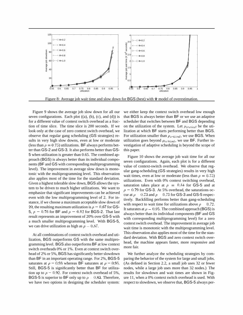
To verify that the assumption that overestimation of jobexecution times indeed do not impact overall system per-formance, we experimented with various values of�. Re-sults are shown in Figure 8. For those plots,BGS with allfour phases and MPL=5 was used. We observe that differ-ences in wait time are insignificant across the entire rangeof utilization. For moderate utilizations of up to 75%, jobslowdown differences are also insignificant. For utiliza-tions of 85% and higher, job slowdown exhibits largervariation with respect to overestimation, but the variationis nonmonotonic and perfect estimation is not necessarilybetter.

5.3 ComparingGS, BGS, and BF

We compare three different scheduling strategies, with atotal of seven configurations. They all use FCFS as theprioritization policy. The first strategy is a space-sharingpolicy that uses backfilling to enhance the performanceparameters. We identify this strategy asBF. We also usethree variations of the gang-scheduling strategy, with mul-tiprogramming levels 2, 3, and 5. These configurationsare identified byGS-2, GS-3, GS-5, respectively. Fi-nally, we consider three configurations of the backfillinggang-scheduling strategy. That is, backfilling is applied toeach virtual machine created by gang-scheduling. Theseare referred to asBGS-2, BGS-3. andBGS-5, for multi-programming level 2, 3, and 5. The results presented hereare based on the�-model, with� = 0:2. We use the per-formance parameters described in Section 2.3, namely (i)average slow down, (ii) average wait time, and (iii) aver-age loss of capacity, to compare the strategies.

0.55 0.6 0.65 0.7 0.75 0.8 0.85 0.9 0.95 10

20

40

60

80

100

120

utilization

Ave

rage

job

slow

dow

n

Φ=0.2

Φ=0.4

Φ=0.6

Φ=0.8

Φ=1.0

0.55 0.6 0.65 0.7 0.75 0.8 0.85 0.9 0.95 10

0.5

1

1.5

2

2.5

3

3.5

4

utilization

Ave

rage

job

wai

t tim

e (X

104 s

econ

ds)

Φ=0.2

Φ=0.4

Φ=0.6

Φ=0.8

Φ=1.0

Figure 8: Average job wait time and slow down forBGS (best) with� model of overestimation.

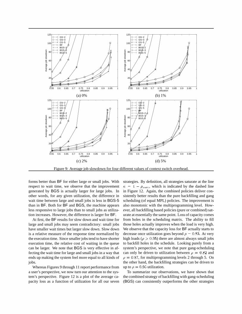
Figure 9 shows the average job slow down for all ourseven configurations. Each plot ((a), (b), (c), and (d)) isfor a different value of context switch overhead as a frac-tion of time slice. The time slice is 200 seconds. If welook only at the case of zero context switch overhead, weobserve that regular gang scheduling (GS strategies) re-sults in very high slow downs, even at low or moderate(less than� = 0:75) utilizations.BF always performs bet-ter thanGS-2 andGS-3. It also performs better thanGS-5 when utilization is greater than 0.65. The combined ap-proach (BGS) is always better than its individual compo-nents (BF andGS with corresponding multiprogramminglevel). The improvement in average slow down is mono-tonic with the multiprogramming level. This observationalso applies most of the time for the standard deviation.Given a highest tolerable slow down,BGS allows the sys-tem to be driven to much higher utilizations. We want toemphasize that significant improvements can be achievedeven with the low multiprogramming level of 2. For in-stance, if we choose a maximum acceptable slow down of20, the resulting maximum utilization is� = 0:67 for GS-5, � = 0:76 for BF and� = 0:82 for BGS-2. That lastresult represents an improvement of 20% overGS-5 witha much smaller multiprogramming level. WithBGS-5,we can drive utilization as high as� = 0:87.

At all combinations of context switch overhead and uti-lization, BGS outperformsGS with the same multipro-gramming level.BGS also outperformsBF at low contextswitch overheads 0% or 1%. Even at context switch over-head of 2% or 5%,BGS has significantly better slowdownthanBF in an important operating range. For 2%,BGS-5saturates at� = 0:93 whereasBF saturates at� = 0:95.Still, BGS-5 is significantly better thanBF for utiliza-tion up to� = 0:92. For context switch overhead of 5%,BGS-5 is superior toBF only up to� = 0:83. Therefore,we have two options in designing the scheduler system:

we either keep the context switch overhead low enoughthatBGS is always better thanBF or we use an adaptivescheduler that switches betweenBF andBGS dependingon the utilization of the system. Let�critical be the uti-lization at whichBF starts performing better thanBGS.For utilization smaller than�critical, we useBGS. Whenutilization goes beyond�critical, we useBF. Further in-vestigation of adaptive scheduling is beyond the scope ofthis paper.

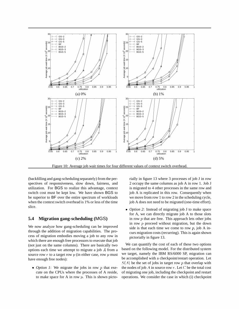
Figure 10 shows the average job wait time for all ourseven configurations. Again, each plot is for a differentvalue of context-switch overhead. We observe that reg-ular gang-scheduling (GS strategies) results in very highwait times, even at low or moderate (less than� = 0:75)utilizations. Even with 0% context switching overhead,saturation takes place at� = 0:84 for GS-5 and at� = 0:79 for GS-3. At 5% overhead, the saturations oc-cur at� = 0:73 and� = 0:75 for GS-3 andGS-5 respec-tively. Backfilling performs better than gang-schedulingwith respect to wait time for utilizations above� = 0:72.It saturates at� = 0:95. The combined approach (BGS) isalways better than its individual components (BF andGSwith corresponding multiprogramming level) for a zerocontext switch overhead. The improvement in average jobwait time is monotonic with the multiprogramming level.This observation also applies most of the time for the stan-dard deviation. WithBGS and zero context switch over-head, the machine appears faster, more responsive andmore fair.

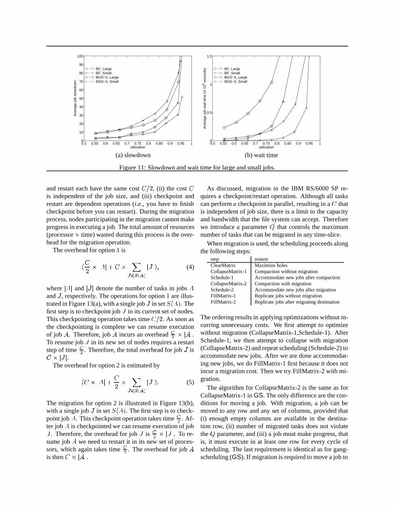
We further analyze the scheduling strategies by com-paring the behavior of the system for large and small jobs.(As defined in Section 2.2, a small job uses 32 or fewernodes, while a large job uses more than 32 nodes.) Theresults for slowdown and wait times are shown in Fig-ure 11, when a 0% context switch overhead is used. Withrespect to slowdown, we observe that,BGS-5 always per-

0.55 0.6 0.65 0.7 0.75 0.8 0.85 0.9 0.95 10

20

40

60

80

100

120

utilization

Ave

rage

job

slow

dow

n

GS−2GS−3GS−5BFBGS−2BGS−3BGS−5

0.55 0.6 0.65 0.7 0.75 0.8 0.85 0.9 0.95 10

20

40

60

80

100

120

utilization

Ave

rage

job

slow

dow

n


(a) 0% (b) 1%

0.55 0.6 0.65 0.7 0.75 0.8 0.85 0.9 0.95 10

20

40

60

80

100

120

utilization

Ave

rage

job

slow

dow

n


0.55 0.6 0.65 0.7 0.75 0.8 0.85 0.9 0.95 10

20

40

60

80

100

120

utilization

Ave

rage

job

slow

dow

n


(c) 2% (d) 5%

Figure 9: Average job slowdown for four different values of context switch overhead.

forms better thanBF for either large or small jobs. Withrespect to wait time, we observe that the improvementgenerated byBGS is actually larger for large jobs. Inother words, for any given utilization, the difference inwait time between large and small jobs is less inBGS-5than inBF. Both for BF andBGS, the machine appearsless responsive to large jobs than to small jobs as utiliza-tion increases. However, the difference is larger forBF.

At first, theBF results for slow down and wait time forlarge and small jobs may seem contradictory: small jobshave smaller wait times but larger slow down. Slow downis a relative measure of the response time normalized bythe execution time. Since smaller jobs tend to have shorterexecution time, the relative cost of waiting in the queuecan be larger. We note thatBGS is very effective in af-fecting the wait time for large and small jobs in a way thatends up making the system feel more equal to all kinds ofjobs.

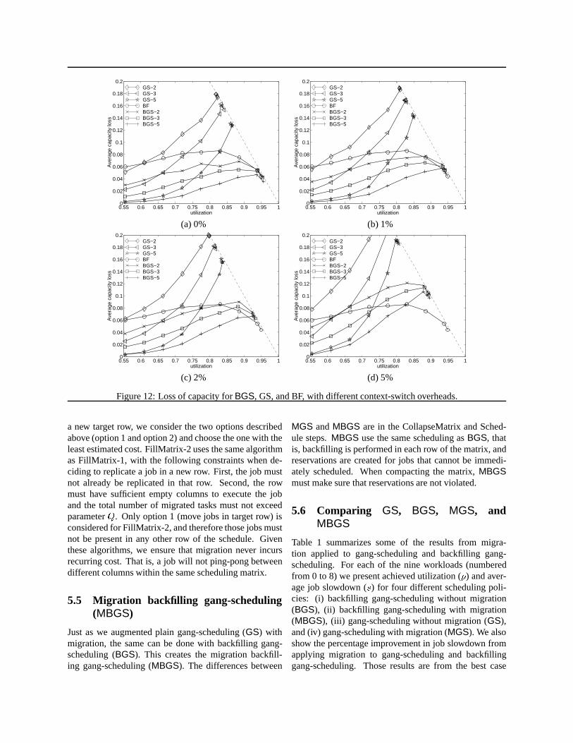
Whereas Figures 9 through 11 report performance froma user’s perspective, we now turn our attention to the sys-tem’s perspective. Figure 12 is a plot of the average ca-pacity loss as a function of utilization for all our seven

strategies. By definition, all strategies saturate at the line� = 1 � �max, which is indicated by the dashed linein Figure 12. Again, the combined policies deliver con-sistently better results than the pure backfilling and gangscheduling (of equal MPL) policies. The improvement isalso monotonic with the multiprogramming level. How-ever, all backfilling based policies (pure or combined) sat-urate at essentially the same point. Loss of capacity comesfrom holes in the scheduling matrix. The ability to fillthose holes actually improves when the load is very high.We observe that the capacity loss forBF actually starts todecrease once utilization goes beyond� = 0:83. At veryhigh loads (� > 0:95) there are almost always small jobsto backfill holes in the schedule. Looking purely from asystem’s perspective, we note that pure gang-schedulingcan only be driven to utilization between� = 0:82 and� = 0:87, for multiprogramming levels 2 through 5. Onthe other hand, the backfilling strategies can be driven toup to� = 0:95 utilization.

To summarize our observations, we have shown thatthe combined strategy of backfilling with gang-scheduling(BGS) can consistently outperforms the other strategies

0.55 0.6 0.65 0.7 0.75 0.8 0.85 0.9 0.95 10

5

10

15

20

25

30

utilization

Ave

rage

job

wai

t tim

e (X

103 s

econ

ds)


0.55 0.6 0.65 0.7 0.75 0.8 0.85 0.9 0.95 10

5

10

15

20

25

30

utilization

Ave

rage

job

wai

t tim

e (X

103 s

econ

ds)


(a) 0% (b) 1%

0.55 0.6 0.65 0.7 0.75 0.8 0.85 0.9 0.95 10

5

10

15

20

25

30

utilization

Ave

rage

job

wai

t tim

e (X

103 s

econ

ds)


0.55 0.6 0.65 0.7 0.75 0.8 0.85 0.9 0.95 10

5

10

15

20

25

30

utilization

Ave

rage

job

wai

t tim

e (X

103 s

econ

ds)


(c) 2% (d) 5%

Figure 10: Average job wait times for four different values of context switch overhead.

(backfilling and gang-scheduling separately) from the per-spectives of responsiveness, slow down, fairness, andutilization. ForBGS to realize this advantage, contextswitch cost must be kept low. We have shownBGS tobe superior toBF over the entire spectrum of workloadswhen the context switch overhead is 1% or less of the timeslice.

5.4 Migration gang-scheduling (MGS)

We now analyze how gang-scheduling can be improvedthrough the addition of migration capabilities. The pro-cess of migration embodies moving a job to any row inwhich there are enough free processors to execute that job(not just on the same columns). There are basically twooptions each time we attempt to migrate a jobA from asource rowr to a target rowp (in either case, rowp musthave enough free nodes):

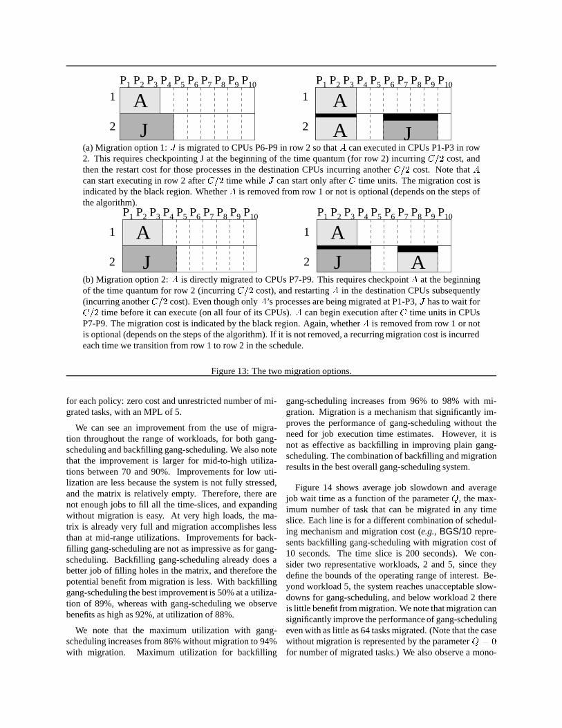
� Option 1: We migrate the jobs in rowp that exe-cute on the CPUs where the processes of A reside,to make space for A in rowp. This is shown picto-

rially in figure 13 where 3 processes of job J in row2 occupy the same columns as job A in row 1. Job Jis migrated to 4 other processes in the same row andjob A is replicated in this row. Consequently whenwe move from row 1 to row 2 in the scheduling cycle,job A does not need to be migrated (one-time effort).

� Option 2: Instead of migrating job J to make spacefor A, we can directly migrate job A to those slotsin row p that are free. This approach lets other jobsin row p proceed without migration, but the downside is that each time we come to rowp, job A in-curs migration costs (recurring). This is again shownpictorially in figure 13.

We can quantify the cost of each of these two optionsbased on the following model. For the distributed systemwe target, namely the IBM RS/6000 SP, migration canbe accomplished with a checkpoint/restart operation. LetS(A) be the set of jobs in target rowp that overlap withthe nodes of jobA in source rowr. LetC be the total costof migrating one job, including the checkpoint and restartoperations. We consider the case in which (i) checkpoint

0.5 0.55 0.6 0.65 0.7 0.75 0.8 0.85 0.9 0.95 10

10

20

30

40

50

60

70

80

90

100

utilization

Ave

rage

job

slow

dow

n

BF, LargeBF, SmallBGS−5, LargeBGS−5, Small

0.5 0.55 0.6 0.65 0.7 0.75 0.8 0.85 0.9 0.95 10

0.5

1

1.5

utilization

Ave

rage

job

wai

t tim

e (X

104 s

econ

ds) BF, Large

BF, SmallBGS−5, LargeBGS−5, Small

(a) slowdown (b) wait time

Figure 11: Slowdown and wait time for large and small jobs.

and restart each have the same costC=2, (ii) the costCis independent of the job size, and (iii) checkpoint andrestart are dependent operations (i.e., you have to finishcheckpoint before you can restart). During the migrationprocess, nodes participating in the migration cannot makeprogress in executing a job. The total amount of resources(processor� time) wasted during this process is the over-head for the migration operation.

The overhead for option 1 is

(C

2� jAj+ C �

X

J2S(A)

jJ j); (4)

wherejAj and jJ j denote the number of tasks in jobsAandJ , respectively. The operations for option 1 are illus-trated in Figure 13(a), with a single jobJ in setS(A). Thefirst step is to checkpoint jobJ in its current set of nodes.This checkpointing operation takes timeC=2. As soon asthe checkpointing is complete we can resume executionof job A. Therefore, jobA incurs an overheadC2 � jAj.To resume jobJ in its new set of nodes requires a restartstep of timeC2 . Therefore, the total overhead for jobJ isC � jJ j.

The overhead for option 2 is estimated by

(C � jAj+C

2�X

J2S(A)

jJ j): (5)

The migration for option 2 is illustrated in Figure 13(b),with a single jobJ in setS(A). The first step is to check-point jobA. This checkpoint operation takes timeC2 . Af-ter jobA is checkpointed we can resume execution of jobJ . Therefore, the overhead for jobJ is C

2 � jJ j. To re-sume jobA we need to restart it in its new set of proces-sors, which again takes timeC2 . The overhead for jobAis thenC � jAj.

As discussed, migration in the IBM RS/6000 SP re-quires a checkpoint/restart operation. Although all taskscan perform a checkpoint in parallel, resulting in aC thatis independent of job size, there is a limit to the capacityand bandwidth that the file system can accept. Thereforewe introduce a parameterQ that controls the maximumnumber of tasks that can be migrated in any time-slice.

When migration is used, the scheduling proceeds alongthe following steps:

step reasonClearMatrix Maximize holesCollapseMatrix-1 Compaction without migrationSchedule-1 Accommodate new jobs after compactionCollapseMatrix-2 Compaction with migrationSchedule-2 Accommodate new jobs after migrationFillMatrix-1 Replicate jobs without migrationFillMatrix-2 Replicate jobs after migrating destination

The ordering results in applying optimizations without in-curring unnecessary costs. We first attempt to optimizewithout migration (CollapseMatrix-1,Schedule-1). AfterSchedule-1, we then attempt to collapse with migration(CollapseMatrix-2) and repeat scheduling (Schedule-2) toaccommodate new jobs. After we are done accommodat-ing new jobs, we do FillMatrix-1 first because it does notincur a migration cost. Then we try FillMatrix-2 with mi-gration.

The algorithm for CollapseMatrix-2 is the same as forCollapseMatrix-1 inGS. The only difference are the con-ditions for moving a job. With migration, a job can bemoved to any row and any set of columns, provided that(i) enough empty columns are available in the destina-tion row, (ii) number of migrated tasks does not violatetheQ parameter, and (iii) a job must make progress, thatis, it must execute in at least one row for every cycle ofscheduling. The last requirement is identical as for gang-scheduling (GS). If migration is required to move a job to

0.55 0.6 0.65 0.7 0.75 0.8 0.85 0.9 0.95 10

0.02

0.04

0.06

0.08

0.1

0.12

0.14

0.16

0.18

0.2

utilization

Ave

rage

cap

acity

loss


0.55 0.6 0.65 0.7 0.75 0.8 0.85 0.9 0.95 10

0.02

0.04

0.06

0.08

0.1

0.12

0.14

0.16

0.18

0.2

utilization

Ave

rage

cap

acity

loss


(a) 0% (b) 1%

0.55 0.6 0.65 0.7 0.75 0.8 0.85 0.9 0.95 10

0.02

0.04

0.06

0.08

0.1

0.12

0.14

0.16

0.18

0.2

utilization

Ave

rage

cap

acity

loss


0.55 0.6 0.65 0.7 0.75 0.8 0.85 0.9 0.95 10

0.02

0.04

0.06

0.08

0.1

0.12

0.14

0.16

0.18

0.2

utilization

Ave

rage

cap

acity

loss


(c) 2% (d) 5%

Figure 12: Loss of capacity forBGS, GS, and BF, with different context-switch overheads.

a new target row, we consider the two options describedabove (option 1 and option 2) and choose the one with theleast estimated cost. FillMatrix-2 uses the same algorithmas FillMatrix-1, with the following constraints when de-ciding to replicate a job in a new row. First, the job mustnot already be replicated in that row. Second, the rowmust have sufficient empty columns to execute the joband the total number of migrated tasks must not exceedparameterQ. Only option 1 (move jobs in target row) isconsidered for FillMatrix-2, and therefore those jobs mustnot be present in any other row of the schedule. Giventhese algorithms, we ensure that migration never incursrecurring cost. That is, a job will not ping-pong betweendifferent columns within the same scheduling matrix.

5.5 Migration backfilling gang-scheduling(MBGS)

Just as we augmented plain gang-scheduling (GS) withmigration, the same can be done with backfilling gang-scheduling (BGS). This creates the migration backfill-ing gang-scheduling (MBGS). The differences between

MGS andMBGS are in the CollapseMatrix and Sched-ule steps.MBGS use the same scheduling asBGS, thatis, backfilling is performed in each row of the matrix, andreservations are created for jobs that cannot be immedi-ately scheduled. When compacting the matrix,MBGSmust make sure that reservations are not violated.

5.6 Comparing GS, BGS, MGS, andMBGS

Table 1 summarizes some of the results from migra-tion applied to gang-scheduling and backfilling gang-scheduling. For each of the nine workloads (numberedfrom 0 to 8) we present achieved utilization (�) and aver-age job slowdown (s) for four different scheduling poli-cies: (i) backfilling gang-scheduling without migration(BGS), (ii) backfilling gang-scheduling with migration(MBGS), (iii) gang-scheduling without migration (GS),and (iv) gang-scheduling with migration (MGS). We alsoshow the percentage improvement in job slowdown fromapplying migration to gang-scheduling and backfillinggang-scheduling. Those results are from the best case

1

2

8 96 PPPPPPPPP1 2 3 4 5 P7 10

A J

A1

2 J

8 96 PPPPPPPPP1 2 3 4 5 P7 10

A

(a) Migration option 1:J is migrated to CPUs P6-P9 in row 2 so thatA can executed in CPUs P1-P3 in row2. This requires checkpointing J at the beginning of the time quantum (for row 2) incurringC=2 cost, andthen the restart cost for those processes in the destination CPUs incurring anotherC=2 cost. Note thatAcan start executing in row 2 afterC=2 time whileJ can start only afterC time units. The migration cost isindicated by the black region. WhetherA is removed from row 1 or not is optional (depends on the steps ofthe algorithm).

1

2

1

2

8 96 PPPPPPPPP1 2 3 4 5 P7 10

A

J

A8 96 PPPPPPPPP1 2 3 4 5 P7 10

J A(b) Migration option 2:A is directly migrated to CPUs P7-P9. This requires checkpointA at the beginningof the time quantum for row 2 (incurringC=2 cost), and restartingA in the destination CPUs subsequently(incurring anotherC=2 cost). Even though onlyA’s processes are being migrated at P1-P3,J has to wait forC=2 time before it can execute (on all four of its CPUs).A can begin execution afterC time units in CPUsP7-P9. The migration cost is indicated by the black region. Again, whetherA is removed from row 1 or notis optional (depends on the steps of the algorithm). If it is not removed, a recurring migration cost is incurredeach time we transition from row 1 to row 2 in the schedule.

Figure 13: The two migration options.

for each policy: zero cost and unrestricted number of mi-grated tasks, with an MPL of 5.

We can see an improvement from the use of migra-tion throughout the range of workloads, for both gang-scheduling and backfilling gang-scheduling. We also notethat the improvement is larger for mid-to-high utiliza-tions between 70 and 90%. Improvements for low uti-lization are less because the system is not fully stressed,and the matrix is relatively empty. Therefore, there arenot enough jobs to fill all the time-slices, and expandingwithout migration is easy. At very high loads, the ma-trix is already very full and migration accomplishes lessthan at mid-range utilizations. Improvements for back-filling gang-scheduling are not as impressive as for gang-scheduling. Backfilling gang-scheduling already does abetter job of filling holes in the matrix, and therefore thepotential benefit from migration is less. With backfillinggang-scheduling the best improvement is 50% at a utiliza-tion of 89%, whereas with gang-scheduling we observebenefits as high as 92%, at utilization of 88%.

We note that the maximum utilization with gang-scheduling increases from 86% without migration to 94%with migration. Maximum utilization for backfilling

gang-scheduling increases from 96% to 98% with mi-gration. Migration is a mechanism that significantly im-proves the performance of gang-scheduling without theneed for job execution time estimates. However, it isnot as effective as backfilling in improving plain gang-scheduling. The combination of backfilling and migrationresults in the best overall gang-scheduling system.

Figure 14 shows average job slowdown and averagejob wait time as a function of the parameterQ, the max-imum number of task that can be migrated in any timeslice. Each line is for a different combination of schedul-ing mechanism and migration cost (e.g., BGS/10 repre-sents backfilling gang-scheduling with migration cost of10 seconds. The time slice is 200 seconds). We con-sider two representative workloads, 2 and 5, since theydefine the bounds of the operating range of interest. Be-yond workload 5, the system reaches unacceptable slow-downs for gang-scheduling, and below workload 2 thereis little benefit from migration. We note that migration cansignificantly improve the performance of gang-schedulingeven with as little as 64 tasks migrated. (Note that the casewithout migration is represented by the parameterQ = 0for number of migrated tasks.) We also observe a mono-

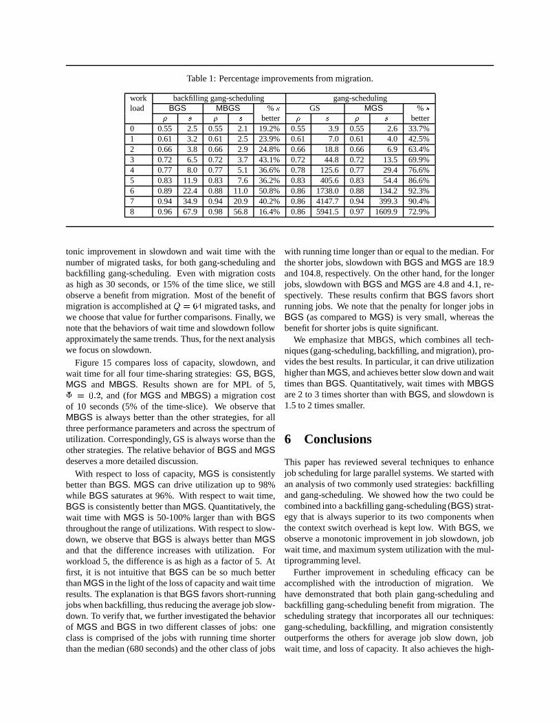
Table 1: Percentage improvements from migration.

work backfilling gang-scheduling gang-schedulingload BGS MBGS % s GS MGS % s

� s � s better � s � s better0 0.55 2.5 0.55 2.1 19.2% 0.55 3.9 0.55 2.6 33.7%1 0.61 3.2 0.61 2.5 23.9% 0.61 7.0 0.61 4.0 42.5%2 0.66 3.8 0.66 2.9 24.8% 0.66 18.8 0.66 6.9 63.4%3 0.72 6.5 0.72 3.7 43.1% 0.72 44.8 0.72 13.5 69.9%4 0.77 8.0 0.77 5.1 36.6% 0.78 125.6 0.77 29.4 76.6%5 0.83 11.9 0.83 7.6 36.2% 0.83 405.6 0.83 54.4 86.6%6 0.89 22.4 0.88 11.0 50.8% 0.86 1738.0 0.88 134.2 92.3%7 0.94 34.9 0.94 20.9 40.2% 0.86 4147.7 0.94 399.3 90.4%8 0.96 67.9 0.98 56.8 16.4% 0.86 5941.5 0.97 1609.9 72.9%

tonic improvement in slowdown and wait time with thenumber of migrated tasks, for both gang-scheduling andbackfilling gang-scheduling. Even with migration costsas high as 30 seconds, or 15% of the time slice, we stillobserve a benefit from migration. Most of the benefit ofmigration is accomplished atQ = 64 migrated tasks, andwe choose that value for further comparisons. Finally, wenote that the behaviors of wait time and slowdown followapproximately the same trends. Thus, for the next analysiswe focus on slowdown.

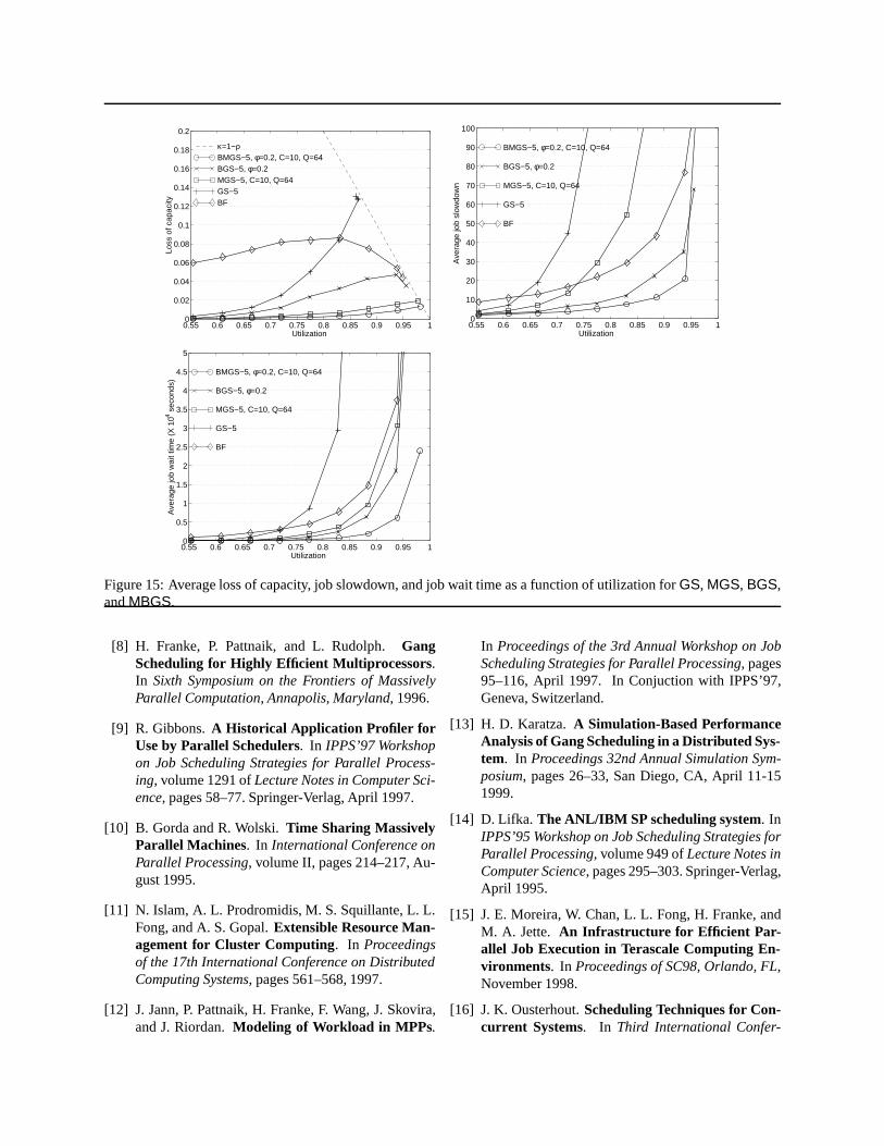
Figure 15 compares loss of capacity, slowdown, andwait time for all four time-sharing strategies:GS, BGS,MGS and MBGS. Results shown are for MPL of 5,� = 0:2, and (forMGS and MBGS) a migration costof 10 seconds (5% of the time-slice). We observe thatMBGS is always better than the other strategies, for allthree performance parameters and across the spectrum ofutilization. Correspondingly, GS is always worse than theother strategies. The relative behavior ofBGS andMGSdeserves a more detailed discussion.

With respect to loss of capacity,MGS is consistentlybetter thanBGS. MGS can drive utilization up to 98%while BGS saturates at 96%. With respect to wait time,BGS is consistently better thanMGS. Quantitatively, thewait time with MGS is 50-100% larger than withBGSthroughout the range of utilizations. With respect to slow-down, we observe thatBGS is always better thanMGSand that the difference increases with utilization. Forworkload 5, the difference is as high as a factor of 5. Atfirst, it is not intuitive thatBGS can be so much betterthanMGS in the light of the loss of capacity and wait timeresults. The explanation is thatBGS favors short-runningjobs when backfilling, thus reducing the average job slow-down. To verify that, we further investigated the behaviorof MGS andBGS in two different classes of jobs: oneclass is comprised of the jobs with running time shorterthan the median (680 seconds) and the other class of jobs

with running time longer than or equal to the median. Forthe shorter jobs, slowdown withBGS andMGS are 18.9and 104.8, respectively. On the other hand, for the longerjobs, slowdown withBGS andMGS are 4.8 and 4.1, re-spectively. These results confirm thatBGS favors shortrunning jobs. We note that the penalty for longer jobs inBGS (as compared toMGS) is very small, whereas thebenefit for shorter jobs is quite significant.

We emphasize that MBGS, which combines all tech-niques (gang-scheduling, backfilling, and migration), pro-vides the best results. In particular, it can drive utilizationhigher thanMGS, and achieves better slow down and waittimes thanBGS. Quantitatively, wait times withMBGSare 2 to 3 times shorter than withBGS, and slowdown is1.5 to 2 times smaller.

6 Conclusions

This paper has reviewed several techniques to enhancejob scheduling for large parallel systems. We started withan analysis of two commonly used strategies: backfillingand gang-scheduling. We showed how the two could becombined into a backfilling gang-scheduling (BGS) strat-egy that is always superior to its two components whenthe context switch overhead is kept low. WithBGS, weobserve a monotonic improvement in job slowdown, jobwait time, and maximum system utilization with the mul-tiprogramming level.

Further improvement in scheduling efficacy can beaccomplished with the introduction of migration. Wehave demonstrated that both plain gang-scheduling andbackfilling gang-scheduling benefit from migration. Thescheduling strategy that incorporates all our techniques:gang-scheduling, backfilling, and migration consistentlyoutperforms the others for average job slow down, jobwait time, and loss of capacity. It also achieves the high-

0 50 100 150 200 250 3000

0.2

0.4

0.6

0.8

1

Maximum number of migrated tasks

Ave

rage

job

wai

t tim

e (X

103 s

econ

ds)

Workload 2, MPL of 5, T = 200 seconds

MGS/0MGS/10MGS/20MGS/30MBGS/0MBGS/10MBGS/20MBGS/30

0 50 100 150 200 250 3000

2

4

6

8

10

12

14

16

18

20


Ave

rage

job

slow

dow

n



0 50 100 150 200 250 3000

0.5

1

1.5

2

2.5

3


Ave

rage

job

wai

t tim

e (X

104 s

econ

ds)



0 50 100 150 200 250 3000

50

100

150

200

250

300

350

400


Ave

rage

job

slow

dow

n



Figure 14: Slowdown and wait time as a function of number of migrated tasks.

est system utilization, allowing the system to reach up to98% utilization. When a maximum acceptable slowdownof 20 is adopted, the system can achieve 94% utilization.

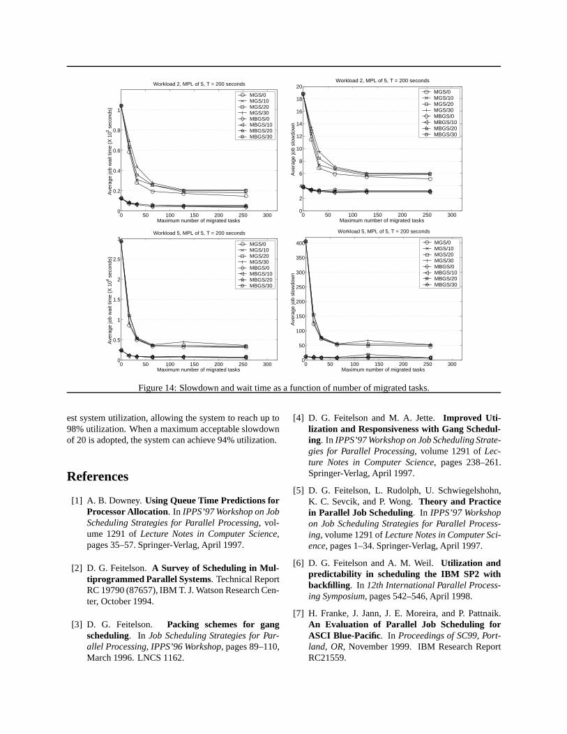
References

[1] A. B. Downey. Using Queue Time Predictions forProcessor Allocation. In IPPS’97 Workshop on JobScheduling Strategies for Parallel Processing, vol-ume 1291 ofLecture Notes in Computer Science,pages 35–57. Springer-Verlag, April 1997.

[2] D. G. Feitelson.A Survey of Scheduling in Mul-tiprogrammed Parallel Systems. Technical ReportRC 19790 (87657), IBM T. J. Watson Research Cen-ter, October 1994.

[3] D. G. Feitelson. Packing schemes for gangscheduling. In Job Scheduling Strategies for Par-allel Processing, IPPS’96 Workshop, pages 89–110,March 1996. LNCS 1162.

[4] D. G. Feitelson and M. A. Jette.Improved Uti-lization and Responsiveness with Gang Schedul-ing. In IPPS’97 Workshop on Job Scheduling Strate-gies for Parallel Processing, volume 1291 ofLec-ture Notes in Computer Science, pages 238–261.Springer-Verlag, April 1997.

[5] D. G. Feitelson, L. Rudolph, U. Schwiegelshohn,K. C. Sevcik, and P. Wong.Theory and Practicein Parallel Job Scheduling. In IPPS’97 Workshopon Job Scheduling Strategies for Parallel Process-ing, volume 1291 ofLecture Notes in Computer Sci-ence, pages 1–34. Springer-Verlag, April 1997.

[6] D. G. Feitelson and A. M. Weil.Utilization andpredictability in scheduling the IBM SP2 withbackfilling . In 12th International Parallel Process-ing Symposium, pages 542–546, April 1998.

[7] H. Franke, J. Jann, J. E. Moreira, and P. Pattnaik.An Evaluation of Parallel Job Scheduling forASCI Blue-Pacific. In Proceedings of SC99, Port-land, OR, November 1999. IBM Research ReportRC21559.

0.55 0.6 0.65 0.7 0.75 0.8 0.85 0.9 0.95 10

0.02

0.04

0.06

0.08

0.1

0.12

0.14

0.16

0.18

0.2

Utilization

Loss

of c

apac

ity

κ=1−ρBMGS−5, φ=0.2, C=10, Q=64BGS−5, φ=0.2MGS−5, C=10, Q=64GS−5BF

0.55 0.6 0.65 0.7 0.75 0.8 0.85 0.9 0.95 10

10

20

30

40

50

60

70

80

90

100

Utilization

Ave

rage

job

slow

dow

n

BMGS−5, φ=0.2, C=10, Q=64

BGS−5, φ=0.2

MGS−5, C=10, Q=64

GS−5

BF

0.55 0.6 0.65 0.7 0.75 0.8 0.85 0.9 0.95 10

0.5

1

1.5

2

2.5

3

3.5

4

4.5

5

Utilization

Ave

rage

job

wai

t tim

e (X

104 s

econ

ds)

BMGS−5, φ=0.2, C=10, Q=64

BGS−5, φ=0.2

MGS−5, C=10, Q=64

GS−5

BF

Figure 15: Average loss of capacity, job slowdown, and job wait time as a function of utilization forGS, MGS, BGS,andMBGS.

[8] H. Franke, P. Pattnaik, and L. Rudolph.GangScheduling for Highly Efficient Multiprocessors.In Sixth Symposium on the Frontiers of MassivelyParallel Computation, Annapolis, Maryland, 1996.

[9] R. Gibbons.A Historical Application Profiler forUse by Parallel Schedulers. In IPPS’97 Workshopon Job Scheduling Strategies for Parallel Process-ing, volume 1291 ofLecture Notes in Computer Sci-ence, pages 58–77. Springer-Verlag, April 1997.

[10] B. Gorda and R. Wolski.Time Sharing MassivelyParallel Machines. In International Conference onParallel Processing, volume II, pages 214–217, Au-gust 1995.

[11] N. Islam, A. L. Prodromidis, M. S. Squillante, L. L.Fong, and A. S. Gopal.Extensible Resource Man-agement for Cluster Computing. In Proceedingsof the 17th International Conference on DistributedComputing Systems, pages 561–568, 1997.

[12] J. Jann, P. Pattnaik, H. Franke, F. Wang, J. Skovira,and J. Riordan.Modeling of Workload in MPPs.

In Proceedings of the 3rd Annual Workshop on JobScheduling Strategies for Parallel Processing, pages95–116, April 1997. In Conjuction with IPPS’97,Geneva, Switzerland.

[13] H. D. Karatza.A Simulation-Based PerformanceAnalysis of Gang Scheduling in a Distributed Sys-tem. In Proceedings 32nd Annual Simulation Sym-posium, pages 26–33, San Diego, CA, April 11-151999.

[14] D. Lifka. The ANL/IBM SP scheduling system. InIPPS’95 Workshop on Job Scheduling Strategies forParallel Processing, volume 949 ofLecture Notes inComputer Science, pages 295–303. Springer-Verlag,April 1995.

[15] J. E. Moreira, W. Chan, L. L. Fong, H. Franke, andM. A. Jette. An Infrastructure for Efficient Par-allel Job Execution in Terascale Computing En-vironments. In Proceedings of SC98, Orlando, FL,November 1998.

[16] J. K. Ousterhout.Scheduling Techniques for Con-current Systems. In Third International Confer-

ence on Distributed Computing Systems, pages 22–30, 1982.

[17] U. Schwiegelshohn and R. Yahyapour.ImprovingFirst-Come-First-Serve Job Scheduling by GangScheduling. In IPPS’98 Workshop on Job Schedul-ing Strategies for Parallel Processing, March 1998.

[18] J. Skovira, W. Chan, H. Zhou, and D. Lifka.TheEASY-LoadLeveler API project . In IPPS’96Workshop on Job Scheduling Strategies for ParallelProcessing, volume 1162 ofLecture Notes in Com-puter Science, pages 41–47. Springer-Verlag, April1996.

[19] W. Smith, V. Taylor, and I. Foster.Using Run-Time Predictions to Estimate Queue Wait Timesand Improve Scheduler Performance. In Proceed-ings of the 5th Annual Workshop on Job Schedul-ing Strategies for Parallel Processing, April 1999.In conjunction with IPPS/SPDP’99, Condado PlazaHotel & Casino, San Juan, Puerto Rico.

[20] K. Suzaki and D. Walsh. Implementation ofthe Combination of Time Sharing and SpaceSharing on AP/Linux. In IPPS’98 Workshop onJob Scheduling Strategies for Parallel Processing,March 1998.

[21] K. K. Yue and D. J. Lilja. Comparing Proces-sor Allocation Strategies in MultiprogrammedShared-Memory Multiprocessors. Journal of Par-allel and Distributed Computing, 49(2):245–258,March 1998.

[22] B. B. Zhou, R. P. Brent, C. W. Jonhson, andD. Walsh.Job Re-packing for Enhancing the Per-formance of Gang Scheduling. In Job SchedulingStrategies for Parallel Processing, IPPS’99 Work-shop, pages 129–143, April 1999. LNCS 1659.

an integrated approach to parallel scheduling using gang-scheduling, backfilling, and migration

Documents