impact of real case transmission systems constraints on wind power operation

Impact of real case transmission systems constraints on windpower operation

Francois Vallee*,y, Jacques Lobry and Olivier Deblecker

Electrical Engineering Department, Universite de Mons, Faculte Polytechnique, Boulevard Dolez, 31 B-7000

Mons, Belgium

SUMMARY

In this paper, a general strategy is proposed in order to introduce in a realistic way wind power into a HLII(bulk power system) nonsequential Monte Carlo adequacy study with economic dispatch. By use of theimplemented solution, wind power can consequently be confronted to operational constraints related tohigh-powered thermal units, nuclear parks or cogeneration. Moreover, in order to optimize the large-scaleintegration of wind power production, the required reinforcements on a given electrical grid can also beevaluated on basis of the presented developments. The elaborated strategy can practically be applied to everykind of nonsequential Monte Carlo approach used to technically analyze a given transmission system. In thecontext of this work, the proposed solution has been implemented into the simulation tool Scanner#(property of Tractebel Engineering – Gaz de France – Suez company). Finally, in order to point out theefficiency and the usefulness of the proposed wind power model, the developed simulation tool has beenfirstly applied to an academic test system: the Roy Billinton test system (RBTS). Afterwards, in order to fullyaccess the large offshore wind potential in the North Sea, the same tool has been used to evaluate the onshorereinforcements required in the Belgian transmission network. Copyright # 2010 John Wiley & Sons, Ltd.

key words: transmission system; wind power; uncertainty; network reinforcement; investments; HLIIreliability

1. INTRODUCTION

EACH investment scenario on a given electrical transmission system must ensure a quality service at

the lowest cost (services continuity, system exploitation, behaviour when facing unexpected outage of

a major element, . . .). In order to answer this major issue of modern networks, it is then necessary to

compute a faithful representation of the transmission system. Therefore, a solution computing a large

number of system states must be developed. In that way, statistical analysis by means of a Monte Carlo

simulation [1–3] can precisely model the electrical system life by sampling a large set of representative

states and consequently permit to obtain coherent exploitation cost and reliability indices for each

studied network.

In a near future, stochastic electrical production and, more specially wind power, is expected to play

an important role in power systems. Therefore, in order to capture the benefits of wind power, the rules

and methods governing the planning and operation of the transmission network need to be optimized to

take into account large-scale power production from wind farms and their locations. In that context,

adequacy studies integrating wind power have been extensively developed for the HLI level (load

covering with always available transmission system) [4,5]. From the bulk power system point of view,

reliability studies taking into account transmission constraints have been introduced in order to

evaluate reinforcements associated to large-scale wind farms integration [6,7]. However, those studies

EUROPEAN TRANSACTIONS ON ELECTRICAL POWEREuro. Trans. Electr. Power 2011; 21:2142–2159Published online 30 December 2010 in Wiley Online Library (wileyonlinelibrary.com). DOI: 10.1002/etep.549

*Correspondence to: Francois Vallee, Electrical Engineering Department, Universite de Mons, Faculte Polytechnique,

Boulevard Dolez, 31 B-7000 Mons, Belgium.yE-mail: [email protected]

Copyright # 2010 John Wiley & Sons, Ltd.

were conducted by use of a sequential Monte Carlo simulation and were thus requiring the use of large

computer resources as the developed wind models were based on complex auto-regressive moving

average (ARMA) time series [6,7]. Moreover, due to the inherent complexity of the sequential

approach, those previous works were not considering eventual operational constraints (fatal

production, nuclear or high powered thermal units that the producer does not want to stop during the

nights . . .) on classical generation units.

In the present study, as reliability and reinforcement analysis are long term studies, a general strategy

is proposed in order to conveniently introduce wind power into a nonsequential Monte Carlo

environment. By the use of such a Monte Carlo method, computing requirements are reduced without

worsening the precision of the obtained global indices (indices of interest in the case of long term

studies). Moreover, due to the greater simplicity of the developed models in the case of a nonsequential

approach, HLII operating and transmission constraints can be simultaneously considered when facing

an increased wind penetration. Therefore, it is believed that the proposed strategy will assist system

planners and transmission system operators to qualitatively assess the system impact of wind power

and to provide adequate input for the managerial decision process in presence of increased wind

penetration. In that way, this strategy has been here implemented into the commercial software

Scanner# (property of Tractebel Engineering – Gaz de France – Suez company) [8] but could

have been applied to each kind of nonsequential Monte Carlo algorithm due to its generality. Finally,

note that the goal of this work is not to study the short term balancing of wind uncertainty (with rapidly

starting coal units) but rather to evaluate reinforcements and long term planning modifications to be

made in order to improve and capture the benefits of wind power.

This paper is organized as follows. In a first part, the nonsequential Monte Carlo approach is

presented in the context of HLII adequacy studies with economical analysis. Then, the methodology

used to introduce wind power in such nonsequential environment is detailed. Thirdly, wind impact on

reliability and reinforcement analysis for transmission systems is computed for an academic test

system: the slightly modified RBTS [9]. In a Section 4, in order to fully access the large offshore wind

potential in the North Sea, the developed simulation tool is used to point out the onshore

reinforcements needed in the Belgian transmission network. Finally, a conclusion is drawn and

summarizes the major results collected after the introduction of wind power into HLII analysis that

takes into account operational and transmission constraints.

2. NONSEQUENTIAL MONTE CARLO SIMULATION IN THE CONTEXT OF HLII

ADEQUACY STUDIES WITH ECONOMICAL ANALYSIS

2.1. System states generation

In this paper, the main objective of the nonsequential Monte Carlo simulation is to provide technical

and economical analysis of development alternatives to be conducted on a given electrical transmission

system (HLII approach). In that way, acceptance (or rejection) criterion is generally based on the

following assessment: ‘Each investment scenario must ensure a quality service (system exploitation,

healthy behaviour when facing unexpected outages, continuity of services . . .) at the lowest cost’. Inorder to efficiently answer this issue, a complete analysis of the investigated system is needed. This

requirement clearly points out the interest of using Monte Carlo simulations as those last ones model

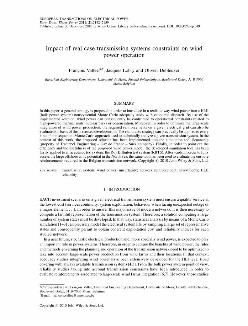
the system evolution as a set of static representative states. Practically, in order to generate the different

system states, a nonsequential Monte Carlo algorithm generally loops on the 52 weeks of the year

(Figure 1).

During each week, a given number (defined by the user according to the required accuracy on the

calculated indices) of hourly system states can be generated by means of the following process:

� Definition of the system state hour during the considered week: Random generation by use of

uniformly distributed numbers on the following fixed interval [0,168] (168 hours during a week);

� For each generated hour: Uniformly distributed random numbers (V) on the interval [0,1] are

sampled for each element (classical generation units, transformers, lines . . .) in order to decide itsoperation state, using the following procedure [2]:

Copyright # 2010 John Wiley & Sons, Ltd. Euro. Trans. Electr. Power 2011; 21:2142–2159DOI: 10.1002/etep

TRANSMISSION GRIDS AND WIND POWER 2143

If V� forced outage rate (FOR that must be interpreted as a probability of unavailability), the

element is considered as unavailable;

If V> FOR, the element is considered as fully available;

Note that, given the considered nonsequential environment, repair time [1] can not be explicitly

defined for classical units. It must rather be implicitly taken into account in the FOR associated to those

classical units. With that kind of approach, it is thus not possible to compute the duration of eventual

load shedding states as a sequential approach would have permitted it. However, if the repair time is

integrated in a global value of the FOR, it will also be possible to define states of load shedding in the

nonsequential approach. Practically, those states will not appear sequentially as the nonsequential

Monte Carlo simulation involves an independency between consecutively generated states.

Nevertheless, at the entire simulation time scale and if the probabilities to be down were well

defined for classical units, accurate global durations of load shedding can still be simulated with the

proposed methodology (the only difference being that this global duration will not be obtained by a set

of sequential hours or states but rather by the addition of nonsequentially defined load shedding states).

Concerning the hourly load at each node of the system, its determination in a nonsequential

approach can be practically based on a random sampling over its cumulative distribution function [2]

or, more precisely, established by the use of modulation diagrams of the annual peak load value [8]:

� Diagram of weekly modulation of the annual peak load: This last one permits to calculate the peak

load of the current week on the basis of the annual peak load value for the considered node. This

diagram contains thus 52 modulation rates of the annual peak load value.

� Diagram of the hourly modulation of the weekly peak load: It permits to calculate the hourly load

for each hour of theweek. This diagram contains thus 24 modulation rates of the weekly peak load

value.

Using this last methodology, no random sampling is needed in order to generate the hourly load at

each node of the system. More easily, the program just considers, in the weekly modulation diagram,

the rate corresponding to the current week during the simulation process (Figure 1). Then, it associates

to the generated weekly peak load the rate of the hourly modulation diagram corresponding to the

investigated hour of the day. Also note that, as the consumption during 1 week can change from one day

to the other (days of the week, Saturday or Sunday), several diagrams of hourly modulation can be

associated to each node during one week. Moreover, seasonal aspects can also be taken into account by

defining periods during the year and by changing the set of hourly modulation diagrams associated to

each node from one period to the other.

Figure 1. General algorithm of the system states generation process in a nonsequential Monte Carloenvironment.


2144 F. VALLEE, J. LOBRY AND O. DEBLECKER

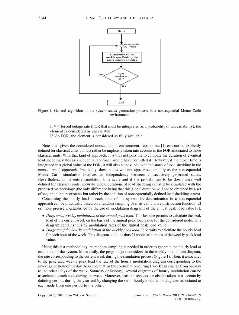
Figure 2a illustrates the load behaviour during 1 year (based on a Belgian real case for the year 2000

[10]) for an annual peak load of 185MWat the considered node. In Figure 2b, a zoom is made on one

week of the year for the same node and illustrates the consideration of possible change of consumption

from one day to the other inside the same week.

2.2. System states analysis

In order to efficiently estimate the investments and eventual reinforcements to be conducted on a given

transmission system, each generated state must then be analyzed. This stage of the process can

practically be achieved by use of three consecutive steps:

(1) Economic dispatch: Generally based on the available production units and done without

considering transmission facilities availability. The objective of this step is to ensure, at the

lowest cost, the hourly load with the available production. Note that an economic dispatch

algorithm can take into account several possible constraints on classical units operation like:

- Hydraulic production and pumping stations: generally considered as a zero cost production

(water is a cheap prime mover) and practically managed at a weekly time scale.

- Thermal production: several types of constraints can be modelled for this kind of production.

Firstly, technical minima (threshold under which the producer does not want to run its unit)

can be considered for technical reasons like desired efficiency . . . Secondly, units like

cogeneration whose electrical production depends on an independent cycle (heat production)

can be modelled using forced units that have a threshold over which they must always operate

when they are available. Finally, in order to take into account high-powered thermal or nuclear

units that the producer does not want to stop during the week, those machines can be

considered as long-term units and must be managed at a weekly time scale. Practically, they

have to run at least at their technical minimum value during the entire week when they are

needed to cover all the reference peak consumptions of that week. Note that, when such a

long-term unit is stopped during oneweek, it can not be started back before the start of the next

week.

Finally, the algorithm that can be conducted during an economic dispatch with integration of

operational constraints over conventional units proceeds as follows. In a first step, hydraulic

production (cheap production cost) must be used to cover the load (following the orders of the

weekly management). Then, technical minimum values of forced and long-term (if they are

required to cover the reference peak loads during the week) thermal units are considered to

satisfy the load (minus hydraulic production). Finally, an economic dispatch of the thermal

production (minus the technical minimum values of already considered forced and long term

units) is realized to cover the remaining load. Note that a disturbance reserve constraint can also

be integrated in the economic dispatch resolution process. Practically, those reserves represent

the fact that the transmission system operator wants to prevent consequences related to the loss

0 1000 2000 3000 4000 5000 6000 7000 80000

20

40

60

80

100

120

140

160

180

200

Time (Hours)

Hou

rly L

oad

(MW

)

Seasonal Modulation of an annual peak load of 185MW

0 20 40 60 80 100 120 140 1600

20

40

60

80

100

120

140

160

180

200

Time (Hours)

Hou

rly L

oad

(MW

)

Hourly modulation over one week of an annual peak load of 185MW

(a) (b)

Figure 2. Seasonal modulation over one year for 185MW peak load value (a) and hourly modulation overone week of the year for the same peak value (b) based on a Belgian real case [10].



of the major unit of the production park. Generally, those reserves are constituted on basis of

already started units or fast starting ones. It is commonly accepted that this reserve must be able

to respond within 15minutes after the production unit outage.

(2) Load flow: When lot of system states are to be analyzed, load flows with alternative current

hypothesis can lead to prohibitive computation times. Consequently, a DC load flow procedure

can be more efficient to choose. Practically, this step carries out the computation of active power

flows in transmission lines without considering reactive power and involves therefore several

high voltage grid hypotheses: bus voltage magnitudes are close to 1 p.u., angular phase shifts

between bus voltages are close to zero and line conductance is always negligible when it is

compared to the susceptance.

In order to economically solve a DC load flow problem, generated active powers calculated

during the economic dispatch must be introduced at the connection nodes of the concerned

parks. Moreover, the generated hourly consumption for the current state must also be taken into

account at the required nodes. DC load flow then computes active power flows over the

transmission system and permits to take into account transmission links constraints. In case of

line overflow, step 3 can eventually be started. On the opposite, if the optimal solution does not

involve overloaded lines, this next step is avoided.

(3) Production rescheduling or load shedding: This step is only useful if the optimal solution of the

economic dispatch leads to overloaded lines during step 2. In that case, the solution is firstly ‘re-

optimized’ in order to avoid those unacceptable situations. Then, if this first stage is not

sufficient to relieve all the overflows, an optimized load shedding procedure can be started in

order to limit active power flows. Practically, the implemented algorithm tends to minimize the

extra cost due to the eventual production rescheduling or load shedding under constraints like

technical minimum power of classical units, power balance equations in buses, maximal power

flows over transmission lines . . .

2.3. Calculated indices and productions

The most significant reliability indices that can be calculated during a technical analysis of a given

transmission grid are certainly the loss of load expectation (LOLE in hours/year) [1] (HLI index

calculated without considering transmission facilities) and the number of hours (per year) of load

shedding (due to transmission overflows). Moreover, hours of overflows are also interesting to compute

for each transmission line in order to point out the weakest points of the system.

Next to those indices, the annual production costs (with andwithout considering elements unavailability)

can also be computed using the implementation of an economical analysis.Moreover,mean production and

annual energy generated by each classical unit are also interesting to calculate. Finally, histograms of

production can be printed out in order to analyze the utilization of each classical unit.

3. INTRODUCTION OFWIND POWER INTOAN HLII NONSEQUENTIAL MONTE CARLO

TECHNICAL AND ECONOMICAL ANALYSIS

Due to the major increase of wind penetration in some countries (like Germany) [11], this variable kind

of production can no more be neglected in technical and economical transmission system analysis.

Therefore, in the present work, wind power has been implemented in such a nonsequential Monte Carlo

simulation tool. In order to achieve that step, modifications related to the introduction of wind have to

impact both major stages of the simulation process: system states generation and the analysis of these

states (Sections 2.1 and 2.2).

3.1. Introduction of wind power in the system states generation process

Before taking into account wind power in the system states generation process, several entities related

to wind power have to be defined. Those ones can be related to wind parks, wind speed regimes and

power curves:

- Wind parks: Each wind park can practically be characterized by its installed capacity, production

cost, FOR of one turbine, associated wind speed regime and power curve [12].



- Wind speed regimes: They are characterized by cumulative distribution functions (CDF) repre-

senting different statistical behaviours for wind speed in the investigated area. Those CDF can be

classicalWeibull distributions [12] or arbitrary ones. In the latter case, distributions can be linearly

interpolated on the joint basis of a wind speed step and probability intervals defined by the user.

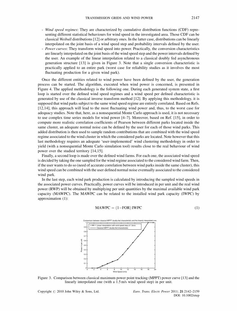
- Power curves: They transform wind speed into power. Practically, the conversion characteristics

are linearly interpolated on the joint basis of thewind speed step and the power intervals defined by

the user. An example of the linear interpolation related to a classical doubly fed asynchronous

generation structure [13] is given in Figure 3. Note that a single conversion characteristic is

practically applied to an entire park (worst case for reliability studies as it involves the most

fluctuating production for a given wind park).

Once the different entities related to wind power have been defined by the user, the generation

process can be started. The algorithm, executed when wind power is concerned, is presented in

Figure 4. The applied methodology is the following one. During each generated system state, a first

loop is started over the defined wind speed regimes and a wind speed per defined characteristic is

generated by use of the classical inverse transform method [12]. By applying this methodology, it is

supposed that wind parks subject to the samewind speed regime are entirely correlated. Based on Refs.

[12,14], this approach will lead to the most fluctuating wind power and, thus, to the worst case for

adequacy studies. Note that, here, as a nonsequential Monte Carlo approach is used, it is not necessary

to use complex time series models for wind power [4–7]. Moreover, based on Ref. [15], in order to

compute more realistic correlation coefficients of Pearson between different parks located inside the

same cluster, an adequate normal noise can be defined by the user for each of those wind parks. This

added distribution is then used to sample random contributions that are combined with the wind speed

regime associated to the wind cluster in which the considered parks are located. Note however that this

last methodology requires an adequate ‘user-implemented’ wind clustering methodology in order to

yield (with a nonsequential Monte Carlo simulation tool) results close to the real behaviour of wind

power over the studied territory [14,15].

Finally, a second loop is made over the defined wind farms. For each one, the associated wind speed

is decided by taking the one sampled for thewind regime associated to the considered wind farm. Then,

if the user wants to do so (need of accurate correlation between wind parks inside the same cluster), this

wind speed can be combined with the user defined normal noise eventually associated to the considered

wind park.

In the last step, each wind park production is calculated by introducing the sampled wind speeds in

the associated power curves. Practically, power curves will be introduced in per unit and the real wind

power (RWP) will be obtained by multiplying per unit quantities by the maximal available wind park

capacity (MAWPC). The MAWPC can be related to the installed wind park capacity (IWPC) by

approximation (1):

MAWPC ¼ ð1�FORÞ IWPC (1)

0 2 4 6 8 10 12 14 16 18 200

0.1

0.2

0.3

0.4

0.5

0.6

0.7

0.8

0.9

1Comparison between classical MPPT doubly-fed characteristic and the linearly interpolated one

Wind Speed (m/s)

Pow

er in

per

uni

t

Linear interpolation with wind speed step of 1.5m/s

Classical MPPT doubly-fed characteristic

Figure 3. Comparison between classical maximum power point tracking (MPPT) power curve [13] and thelinearly interpolated one (with a 1.5m/s wind speed step) in per unit.



By applying (1), possible outages of wind turbines inside a park are approached. However, this

hypothesis leads to acceptable results for high-powered wind parks connected to transmission systems

as those last ones will be practically composed of a large number of turbines.

Alternatively, note that the state of each individual wind turbine can be more precisely defined by

sampling uniform random numbers and comparing it to the turbine FOR (generalization of the

sampling procedure used to define the state of each classical park; cf. Section 2.1 [1]). Finally, by

adding the capacity of each available turbine, a more accurate value of MAWPC is obtained via this

second method. Nevertheless, this approach is less immediate than the one based on Equation (1).

The described wind power sampling process must be started back for each system state.

Consequently, a Generated Wind Power Distribution can be plotted at the end of the Monte Carlo

simulation for each wind park ‘i’.

Figure 5 illustrates the obtained wind power distribution for one 8MW wind farm subject to a

Weibull wind speed regime (with scale parameter A¼ 9.25 and shape parameter B¼ 2.15) and using a

maximum power point tracking (MPPT) power curve similar to the one depicted in Figure 3. Note that

Figure 4. Algorithm of wind power sampling during each system state.

0 1 2 3 4 5 6 7 80

0.05

0.1

0.15

0.2

0.25

0.3

0.35

0.4

0.45

Power (MW)

Pro

babi

lity

Annual distribution of generated wind production for a 8MW wind park (A = 9.25 and B = 2.15)

Figure 5. Simulated annual distribution of generated wind power for a 8MW wind park (A¼ 9.25 andB¼ 2.15).



the increase of probability observed in Figure 5 near the installed capacity is due to the power

limitation (at nominal power) usually applied in variable speed wind power units for wind speeds

located between rated and cut out values [13].

3.2. Introduction of wind power in system states analysis

The generated wind power (GWPi) represents thus, for each defined park ‘i’, the sampled wind power

during the simulated system state. This power must then be taken into account in the system state

analysis.

The introduction of wind power into an economic dispatch algorithm has so been based on several

starting hypotheses (return of experience):

- Hypothesis 1: It has been considered that wind power was not accurately predictable at the weekly

time scale [11] and could therefore not impact the management of hydraulic and long term thermal

(nuclear) units. Those classical units must thus be still processed at the weekly time scale without

taking into account wind impact.

- Hypothesis 2: Wind power is considered as a must run production with zero cost. This hypothesis

is based on the multiple encouraging policies that generally support wind power [16,17].

Consequently, in the economic dispatch, wind power will be directly considered after the

technical constraints related to forced and ‘having to run’ long-term thermal units.

- Hypothesis 3: In case of increased wind penetration, the transmission system operator (TSO) can

be forced (like it has already been the case in some German places [18]) to cut some wind power

when facing conventional parks operating constraints [18]. In the proposed algorithm, when

encountering such situations, wind power is decreased, for each wind park, proportionally to its

available generated power.

- Hypothesis 4: As already mentioned in Section 2.2, dimensioning the disturbance reserve is

commonly based on the largest unit tripping off instantaneously [19]. In that way, it can be

considered [19] that wind power has no influence on the disturbance reserve as long as installed

wind farms are less than the largest production unit in the system (which is still the case in the

majority of countries). It has thus been supposed in this paper that the current wind penetration

levels were not affecting the disturbance reserve. Concerning the short-term (several minutes)

operational reserves used to balance wind power fluctuations, they are beyond the scope of this

study (Section 1) as the investigated states are supposed to be steady-state hourly ones.

- Hypothesis 5: Concerning power quality and more specially voltage control with wind power, it is

important to quote that the initial Scanner# algorithm is based on very high voltage (�150 kV)

network hypotheses (Section 2.2). For very high voltage lines, their reactance X can practically be

considered 10 times greater than their resistance R (X� 10R) [20] and the classical expression (2)

of the voltage drop in the line DV can be simplified to (3) [20]:

DV ¼ RPþ XQ

V2

(2Þ

DV ¼ XQ

V2

(3Þwhere, P and Q are, respectively, the active and reactive power flowing in the line, V1 and V2 the

voltages, respectively, at generator and load connection nodes.

The active power generated by wind turbines is, by definition, highly fluctuating. By con-

sequence, at the distribution level and based on Equation (2), it involves voltage fluctuations in the

network area close to the connection nodes of wind turbines. In transmission grids with very high

voltage lines, Equation (3) shows that voltage variations are essentially due to reactive power flows

(on the opposite to distribution networks). Therefore, wind turbines currently connected to the

transmission network must participate to the voltage control by means of a reactive power control.

Given the recent developments in power electronics, this control is possible with the in-vogue

doubly fed asynchronous or synchronous wind generators [20]. Based on those conclusions, it has

been supposed in our developments that wind generators were able to entirely participate to the



voltage control and that the hypotheses related to the application of the DC load flow (bus voltage

magnitudes are close to 1 p.u., angular phase shifts between bus voltages are close to zero; Section

2.2) were still applicable after the introduction of wind power in the Scanner# algorithm.

- Hypothesis 6: Stability aspects like transient stability, fault ride through capability, voltage flicker

resulting from wind turbulence are of major importance when connecting a wind farm to the

transmission grid. In that way, when assessing the wind farm stability, wind generators technol-

ogies (doubly fed induction wind generator, squirrel cage induction wind generator, converter-

driven synchronous wind generator, directly coupled synchronous wind generator, . . .), windconditions and the short circuit ratio (SCR¼ short circuit power at the connection bus divided by

the wind farm nominal power) at the point of common coupling (PCC) have a high importance.

The SCR ratio can practically vary from very low values (SCR� 2) that can be found in some

remote areas in the USA or Australia [21] to higher values (SCR� 20) for ‘strong networks’ like

most of the European grids [21]. Refs. [21,22] propose a complete study of the combined impact of

SCR and wind generator technology. In that way, it is shown that variable speed wind generators

(DFIWG, CDSWG, DCSWG, . . .) provide a good transient stability in most cases (for both strong

and weak networks), the only problematic situations coming from strong wind situations in some

remote areas with a very low SCR. On the opposite, [22] clearly observes that wind farm stability

with fixed speed wind generators (SCIWG) strongly depends on the short circuit power at the

connection buses and that, in order to ensure a sufficient power quality, the SCR of the weakest

buses must reach at least values greater than 20 with that kind of wind generators.

Power system reliability evaluation is an important part of various facilities planning, such as

generation, transmission and distribution networks. Practically, power system reliability can be

described by two important attributes: adequacy and security. Adequacy is the measure of a power

system to satisfy the consumer demand in all steady state conditions and does therefore not include

system disturbances. On the opposite, security is the measure of the system ability to withstand a

sudden and severe disturbance while maintaining system integrity. Security is consequently

associated with the system response to different disturbances and quantifies therefore stability

aspects like transient stability or fault ride through capability . . . In this paper, the main objective

of Scanner# is to provide a technical (and economical) analysis based on the adequacy evaluation

of the investigated transmission system as each generated hourly state is supposed to be a steady

one (Section 2.1). As a consequence, transient stability aspects are not under the scope of

Scanner# and the impact of an eventual SCR increase (by an adequate planning of new power

lines or by increasing the meshing of the transmission grid . . .) in order to improve the wind farm

stability can not be evaluated with the Scanner# software.

The existence of some transmission system operation constraints can thus lead to a reduction of the

real produced wind power. Therefore, in the developed algorithm, two quantities related to wind power

have been defined for each wind park:

- Real wind power: It represents the real produced wind power after having taken into account the

economic dispatch. A single RWPi value is associated to each wind park ’i’;

- Lost wind power (LWP): It defines the difference between the generated wind power and the real

produced one for each considered wind park. A single LWPi value is thus calculated for each wind

park ‘i’.

The algorithm, implemented in order to take into account wind power in the economic dispatch

associated to each generated system state, is described in Figure 6.

Based on hypotheses 1 and 2, wind power is thus used to cover the remaining load after that

hydraulic production and technical minima of forced and ‘must run’ long term thermal parks (Section

2.2) have been taken into account. If this remaining load L1 is equal to zero, all the hourly load has

already been covered before considering wind power. In that case, real transmitted wind power RWPi is

set to zero for each wind park ‘i’ and their associated lost wind power LWPi equals their initially GWPiduring the considered system state.

On the other hand, if the remaining load L1 is greater than zero, global generated wind power

(GGWP) is taken into account before the remaining classical thermal production (without constraints)



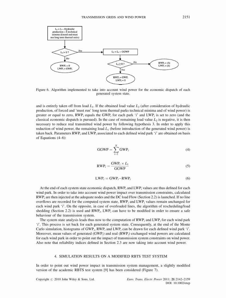
and is entirely taken off from load L1. If the obtained load value L2 (after consideration of hydraulic

production, of forced and ‘must run’ long term thermal parks technical minima and of wind power) is

greater or equal to zero, RWPi equals the GWPi for each park ‘i’ and LWPi is set to zero (and the

classical economic dispatch is pursued). In the case of remaining load value L2 is negative, it is then

necessary to reduce real transmitted wind power by following hypothesis 3. In order to apply this

reduction of wind power, the remaining load L1 (before introduction of the generated wind power) is

taken back. Parameters RWPi and LWPi associated to each defined wind park ‘i’ are obtained on basis

of Equations (4–6):

GGWP ¼XN

i¼1

GWPi (4)

RWPi ¼ GWPi � L1

GGWP(5)

LWPi ¼ GWPi�RWPi (6)

At the end of each system state economic dispatch, RWPi and LWPi values are thus defined for each

wind park. In order to take into account wind power impact over transmission constraints, calculated

RWPi are then injected at the adequate nodes and the DC load Flow (Section 2.2) is launched. If no line

overflows are recorded for the computed system state, RWPi and LWPi values remain unchanged for

each wind park ‘i’. On the opposite, in case of overloaded lines, the algorithm of rescheduling/load

shedding (Section 2.2) is used and RWPi, LWPi can have to be modified in order to ensure a safe

behaviour of the transmission system.

The system state analysis leads thus now to the computation of RWPi and LWPi for each wind park

‘i’. This process is set back for each generated system state. Consequently, at the end of the Monte

Carlo simulation, histograms of GWPi, RWPi and LWPi can be drawn for each defined wind park ‘i’.

Moreover, mean values of generated (GWPi) and real (RWPi) exchanged wind powers are calculated

for each wind park in order to point out the impact of transmission system constraints on wind power.

Also note that reliability indices defined in Section 2.3 are now taking into account wind power.

4. SIMULATION RESULTS ON A MODIFIED RBTS TEST SYSTEM

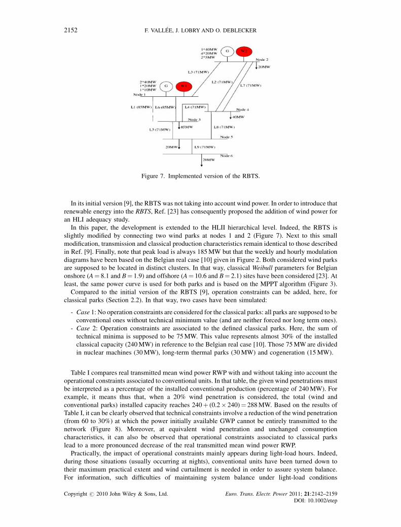
In order to point out wind power impact in transmission system management, a slightly modified

version of the academic RBTS test system [9] has been considered (Figure 7).

Figure 6. Algorithm implemented to take into account wind power for the economic dispatch of eachgenerated system state.



In its initial version [9], the RBTS was not taking into account wind power. In order to introduce that

renewable energy into the RBTS, Ref. [23] has consequently proposed the addition of wind power for

an HLI adequacy study.

In this paper, the development is extended to the HLII hierarchical level. Indeed, the RBTS is

slightly modified by connecting two wind parks at nodes 1 and 2 (Figure 7). Next to this small

modification, transmission and classical production characteristics remain identical to those described

in Ref. [9]. Finally, note that peak load is always 185MW but that the weekly and hourly modulation

diagrams have been based on the Belgian real case [10] given in Figure 2. Both considered wind parks

are supposed to be located in distinct clusters. In that way, classical Weibull parameters for Belgian

onshore (A¼ 8.1 and B¼ 1.9) and offshore (A¼ 10.6 and B¼ 2.1) sites have been considered [23]. At

least, the same power curve is used for both parks and is based on the MPPT algorithm (Figure 3).

Compared to the initial version of the RBTS [9], operation constraints can be added, here, for

classical parks (Section 2.2). In that way, two cases have been simulated:

- Case 1: No operation constraints are considered for the classical parks: all parks are supposed to be

conventional ones without technical minimum value (and are neither forced nor long term ones).

- Case 2: Operation constraints are associated to the defined classical parks. Here, the sum of

technical minima is supposed to be 75MW. This value represents almost 30% of the installed

classical capacity (240MW) in reference to the Belgian real case [10]. Those 75MWare divided

in nuclear machines (30MW), long-term thermal parks (30MW) and cogeneration (15MW).

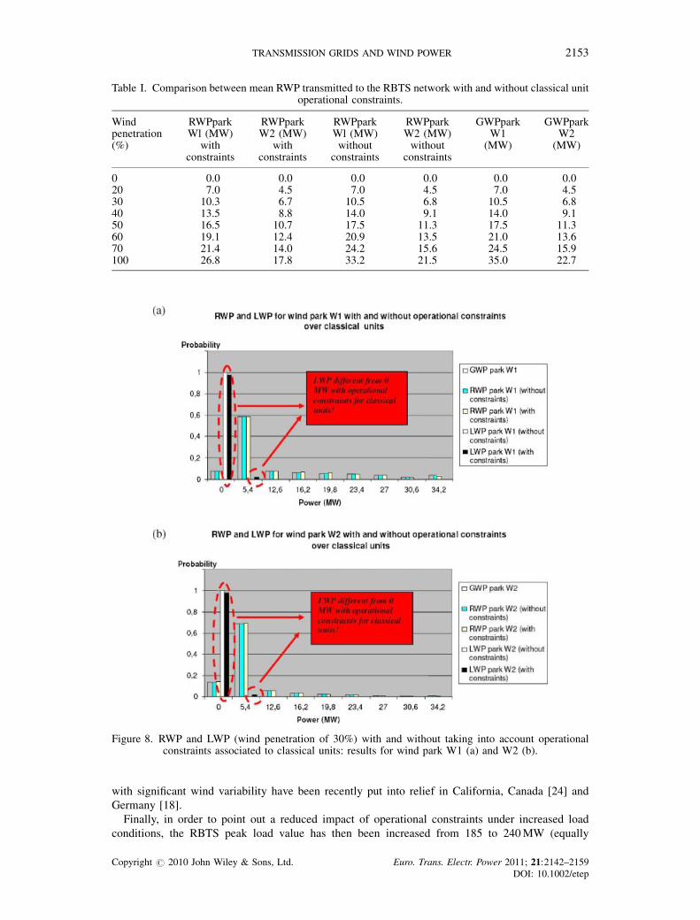
Table I compares real transmitted mean wind power RWP with and without taking into account the

operational constraints associated to conventional units. In that table, the given wind penetrations must

be interpreted as a percentage of the installed conventional production (percentage of 240MW). For

example, it means thus that, when a 20% wind penetration is considered, the total (wind and

conventional parks) installed capacity reaches 240þ (0.2� 240)¼ 288MW. Based on the results of

Table I, it can be clearly observed that technical constraints involve a reduction of the wind penetration

(from 60 to 30%) at which the power initially available GWP cannot be entirely transmitted to the

network (Figure 8). Moreover, at equivalent wind penetration and unchanged consumption

characteristics, it can also be observed that operational constraints associated to classical parks

lead to a more pronounced decrease of the real transmitted mean wind power RWP.

Practically, the impact of operational constraints mainly appears during light-load hours. Indeed,

during those situations (usually occurring at nights), conventional units have been turned down to

their maximum practical extent and wind curtailment is needed in order to assure system balance.

For information, such difficulties of maintaining system balance under light-load conditions

Figure 7. Implemented version of the RBTS.



with significant wind variability have been recently put into relief in California, Canada [24] and

Germany [18].

Finally, in order to point out a reduced impact of operational constraints under increased load

conditions, the RBTS peak load value has then been increased from 185 to 240MW (equally

Table I. Comparison between mean RWP transmitted to the RBTS network with and without classical unitoperational constraints.

Windpenetration(%)

RWPparkWl (MW)

withconstraints

RWPparkW2 (MW)

withconstraints

RWPparkWl (MW)without

constraints

RWPparkW2 (MW)without

constraints

GWPparkW1

(MW)

GWPparkW2

(MW)

0 0.0 0.0 0.0 0.0 0.0 0.020 7.0 4.5 7.0 4.5 7.0 4.530 10.3 6.7 10.5 6.8 10.5 6.840 13.5 8.8 14.0 9.1 14.0 9.150 16.5 10.7 17.5 11.3 17.5 11.360 19.1 12.4 20.9 13.5 21.0 13.670 21.4 14.0 24.2 15.6 24.5 15.9100 26.8 17.8 33.2 21.5 35.0 22.7

Figure 8. RWP and LWP (wind penetration of 30%) with and without taking into account operationalconstraints associated to classical units: results for wind park W1 (a) and W2 (b).



distributed between the five initial load nodes). In that case, the mean gap between operational

constraints (unchanged) and light-load hours is increased. Therefore, an increased (from 30 to 40%)

borderline wind penetration can also be logically observed in Table II. Nevertheless, if increasing the

load improves the use of available wind energy under operational constraints related to conventional

units, it implies larger power flows over the unchanged RBTS system. Consequently, in that scenario, it

is not surprising to observe local load shedding situations at node 3 (Table II). Note that the wind

penetrations given in Table II must again be interpreted as a percentage of the installed conventional

production (percentage of 240MW). Therefore, by increasing the wind penetration, the total (wind and

conventional units) installed capacity is thus also increased which logically leads to reduced values of

LOLE (as the load characteristics are unchanged for the different considered wind penetrations) in

Table II. Moreover, the decreased number of load shedding hours, observed when wind penetration is

increased, is explained by the fact that the complementary wind power installed at node 2 can be

transmitted to sensitive node 3 without overloading the critic lines L1 and L6. Consequently, when

increasing the wind power installed at node 2, the number of load shedding hours at node 3 (due to

overflows on line L1 or L6) is decreased.

The results proposed in this section point out the utility of the proposed models in order to improve

the long-term management of wind power. Indeed, using this tool, transmission system operators will

now be able to calculate the maximal wind penetration before meeting wind power decrease under

light-load conditions.

5. INVESTMENTS STUDY FOR THE BELGIAN TRANSMISSION SYSTEM

In this paragraph, the proposed nonsequential Monte Carlo simulation tool is applied to the real case

Belgian transmission system. As illustrated in Figure 9, this last one is highly interconnected and its

topology can be practically explained by historical considerations. Indeed, along time, the voltage

magnitude of the installed connections has been continuously increased from 36 towards 380 kV.

Those new links have been systematically integrated in the already existing infrastructures and have

consequently led to a highly interconnected Belgian transmission system. By the end 2007, the Belgian

transmission network consisted so in 8406 km of high voltage links. The practical distribution of those

lines is given in Table III and points out that the major part of the Belgian network is comprised

between 70 and 150 kV [25].

In the early 2009, the installed production capacity connected to the Belgian transmission system

was reaching 16.322GW. This maximal power was practically produced by nuclear (6550.5MW),

thermal1 (7914.6MW) and cogeneration (692.9MW) units. Also note that pumping stations are

installed in Belgium for 1164MW capacity. Concerning the Belgian consumption, the peak load value

(considering the decentralized production connected to the distribution network) was about

14.033GW by the end 2008 [26].

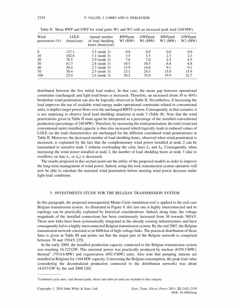
Table II. Mean RWP and GWP for wind parks W1 and W2 with an increased peak load (240MW).

Windpenetration (%)

LOLE(hour/year)

Annual numberof load sheddinghours (hour/year)

RWPparkWl (MW)

GWPparkWl (MW)

RWPparkW2 (MW)

GWPparkW2 (MW)

0 137.1 3.5 (node 3) 0.0 0.0 0.0 0.010 102.6 3.1 (node 3) 3.5 3.5 2.3 2.320 78.5 2.9 (node 3) 7.0 7.0 4.5 4.530 61.3 2.8 (node 3) 10.5 10.5 6.8 6.840 50.4 2.7 (node 3) 13.9 14.0 9.1 9.170 30.4 2.5 (node 3) 23.1 24.5 15.0 15.9100 22.0 2.4 (node 3) 30.5 35.0 19.9 22.7

1Combined cycle units, coal thermal parks, diesel and turbo-jet units are included in this category.



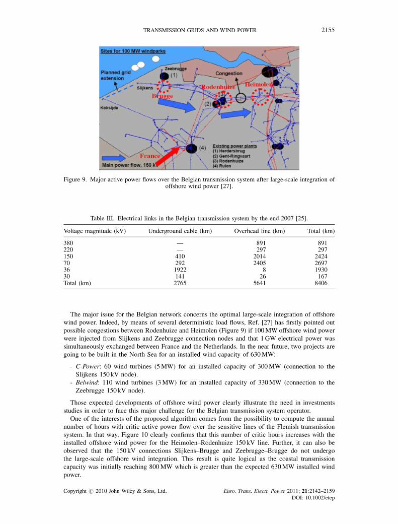
The major issue for the Belgian network concerns the optimal large-scale integration of offshore

wind power. Indeed, by means of several deterministic load flows, Ref. [27] has firstly pointed out

possible congestions between Rodenhuize and Heimolen (Figure 9) if 100MW offshore wind power

were injected from Slijkens and Zeebrugge connection nodes and that 1GW electrical power was

simultaneously exchanged between France and the Netherlands. In the near future, two projects are

going to be built in the North Sea for an installed wind capacity of 630MW:

- C-Power: 60 wind turbines (5MW) for an installed capacity of 300MW (connection to the

Slijkens 150 kV node).

- Belwind: 110 wind turbines (3MW) for an installed capacity of 330MW (connection to the

Zeebrugge 150 kV node).

Those expected developments of offshore wind power clearly illustrate the need in investments

studies in order to face this major challenge for the Belgian transmission system operator.

One of the interests of the proposed algorithm comes from the possibility to compute the annual

number of hours with critic active power flow over the sensitive lines of the Flemish transmission

system. In that way, Figure 10 clearly confirms that this number of critic hours increases with the

installed offshore wind power for the Heimolen–Rodenhuize 150 kV line. Further, it can also be

observed that the 150 kV connections Slijkens–Brugge and Zeebrugge–Brugge do not undergo

the large-scale offshore wind integration. This result is quite logical as the coastal transmission

capacity was initially reaching 800MW which is greater than the expected 630MW installed wind

power.

Figure 9. Major active power flows over the Belgian transmission system after large-scale integration ofoffshore wind power [27].

Table III. Electrical links in the Belgian transmission system by the end 2007 [25].

Voltage magnitude (kV) Underground cable (km) Overhead line (km) Total (km)

380 — 891 891220 — 297 297150 410 2014 242470 292 2405 269736 1922 8 193030 141 26 167Total (km) 2765 5641 8406



In order to improve the offshorewind integration and, consequently, to reduce the active power flows

over the Rodenhuize–Heimolen line, the proposed solution has consisted in an additional 150MW grid

extension between Koksijde and Slijkens. Using this new line, simulation results (Figure 11) obtained

with a 1GW power exchange between France and the Netherlands point out a decrease of critic power

flows on the Rodenhuize–Heimolen connection. This result can be easily explained as a fraction of the

transmitted wind power is now deflected towards Koksijde.

However, after an increase to 2GWof the electricity exchange between France and the Netherlands,

a large decrease of the transmitted wind energy (Figure 12a) but also a dramatic increase of critic power

flows between Rodenhuize and Heimolen (Figure 12b) can be observed with the developed simulation

tool.

Consequently, in the context of largely interconnected European transmission systems, it will be

imperative to imagine new reinforcements in the Belgian network. In that way, one of the possible

solutions could come from the splitting of the Rodenhuize–Heimolen line. Indeed, in that case,

Figure 13 shows a decrease of the simulated annual number of critic hours on this connection even if

the power exchange between France and the Netherlands is set to 2GW.

Finally, the previous simulation results clearly confirm the applicability of the proposed algorithm in

order to evaluate reinforcements and long term planning modifications to improve and capture the

benefits of wind power in transmission systems.

Figure 10. Critic hours (active power greater than 80% of line capacity) over major transmission lines in theFlemish high voltage system. Impact of the offshore wind power.

Figure 11. Critic hours (active power greater than 90% of line capacity) over Rodenhuize–Heimolen linewith and without the added grid extension.



6. CONCLUSIONS

In this paper, wind power has been implemented into a transmission system technical and economical

analysis. In that way, a general strategy has been proposed in order to conveniently implement wind

power in a nonsequential Monte Carlo simulation tool that computes the investments to be conducted

on a given transmission grid. Finally, a useful HLII analysis tool that takes into account wind power has

Figure 12. Impact of the import level between France and the Netherlands on the offshore wind loss ofenergy (a) and on the power flows between Rodenhuize and Heimolen (b).

Figure 13. Impact of Rodenhuize–Heimolen splitting on critic power flows over the Belgian transmissionsystem.



been developed and has permitted to study the impact of operational and power flow constraints over

large-scale wind integration. In that way, situations of forced wind stopping were pointed out under

operational constraints due to an increased wind penetration and light-load hours. Moreover, based on

the proposed simulation tool, adequate reinforcements on the Belgian transmission system could also

be evaluated in order to ensure an optimal integration of the expected offshore wind power. Finally, it is

therefore believed that the proposed solution will assist system planners and transmission system

operators to qualitatively assess the system impact of wind power and to provide adequate input for the

managerial decision process in presence of increased wind penetration.

7. LIST OF ABBREVIATIONS

CDSWG converter driven synchronous wind generator

DCSWG directly coupled synchronous wind generator

DFIWG doubly-fed induction wind generator

FOR forced outage rate

GWP generated wind power

HLI hierarchical level I

HLII hierarchical level II

IWPC installed wind park capacity

LOLE loss of load expectation

LWP lost wind power

MAWPC maximal available wind park capacity

PCC point of common coupling

RWP real wind power

SCR short circuit ratio

ACKNOWLEDGEMENTS

The authors gratefully acknowledge the contributions of S. Rapoport, K. Karoui and M. Stubbe from TractebelEngineering – Gaz de France – Suez for the support given to this work.

REFERENCES

1. Billinton R, Chen H, Ghajar R. A sequential simulation technique for adequacy evaluation of generating systems

including wind energy. IEEE Transactions on Energy Conversion 1996; 11(4): 728–734.2. Papaefthymiou G, Schavemaker PH, Van der Sluis L, Kling WL, Kurowicka D, Cooke RM. Integration of

stochastic generation in power systems. International Journal of Electrical Power & Energy Systems 2006;

18(9): 655–667.3. Bagen W, Billinton R. Incorporating well-being considerations in generating systems using energy storage. IEEE

Transactions on Energy Conversion 2005; 20(1): 225–230.4. Billinton R, Bai G. Generating capacity adequacy associated with wind energy. IEEE Transactions on Energy

Conversion 2004; 19(3): 641–646.5. Wangdee W, Billinton R. Considering load-carrying capability and wind speed correlation of WECS in generation

adequacy assessment. IEEE Transactions on Energy Conversion 2006; 21(3): 734–741.6. Billinton R, Wangdee W. Reliability-based transmission reinforcement planning associated with large-scale wind

farms. IEEE Transactions on Power Systems 2007; 22(1): 34–41.7. TradeWind Project. Integrating wind: developing Europe’s power market for the large-scale integration of wind

power, EWEA, Feb. 2009.

8. Scanner# Software. 1989; In-house developed software. Informations: www.archives-suez.com/document/

?f=presse/en/up1639.pdf.

9. Billinton R, Kumar S, Chowdhury N, et al. A reliability test system for educational purposes – basic data. IEEE

Transactions on Power Systems 1989; 4(3): 1238–1244.10. Buyse H. Electrical energy production, Electrabel doc., available at: www.lei.ucl.ac.be/�matagne/ELEC2753/

SEM12/S12TRAN.PPT 2004.

11. Ernst B. Wind power forecast for the German and Danish networks. In Wind Power in Power Systems, chapter 17,

Ackerman Thomas (ed). John Wiley & Sons: Chichester, England, 2005; 365–381.



12. Vallee F, Lobry J, Deblecker O. System reliability assessment method for wind power integration. IEEE Transactions

on Power Systems 2008; 23(3): 1288–1297.13. Al Aimani S. Modelisation de differentes technologies d’eoliennes integrees a un reseau de distribution moyenne

tension, Ph.D. Thesis, Ecole Centrale de Lille, chap.2, pp.24-25, December 2004.

14. Papaefthymiou G. Integration of stochastic generation in power systems, PhD. Thesis, Delft University, chapters 5 &

6, June 2006.

15. Vallee F, Lobry J, Deblecker O. Application and comparison of wind speed sampling methods for wind generation in

reliability studies using non-sequential Monte Carlo simulations. European Transactions on Electrical Power 2009;

19(7): 1002–1015.16. Mackensen R, Lange B, Schlogl F. Integrating wind energy into public power supply systems – German state of the

art. International Journal of Distributed Energy Sources 2007; 3(4): pp.259-271.17. Maupas F. Analyse des regles de gestion de la production eolienne : inter-comparaison de trois cas d’etude au

Danemark, en Espagne et en Allemagne, Working paper, GRJM Conference, February 2006.

18. Sacharowitz S. Managing large amounts of wind generated power feed in – every day challenges for a German TSO

and approaches for improvements. International Association for Energy Economics (IAEE), 2004 North American

Conference, Washington DC, USA, 2004.

19. Holttinen H. The impact of large scale wind power production on the Nordic electricity system, Doctor of Science

Thesis, Department of Electrical Engineering, Helsinki University of Technology, Finland, December 2004.

20. Robyns B, Davigny A, Saudemont C, et al. Impact de l’eolien sur le reseau de transport et la qualite de l’energie,

revue J3eA, vol. 5, Hors serie no. 1, 2006.

21. Muller H, Poller M, Basteck A, Tilscher A, Pfister J. Grid compatibility of variable speed wind turbines with directly

coupled synchronous generator and hydro-dynamically controlled gearbox, 6th International Workshop on Large

Scale Integration of Wind Power and Transmission Networks for Offshore Wind Farms, Delft, The Netherlands, 26–

28 October, pp. 307–315, 2006.

22. Ledesma P, Usaola J, Rodriguez JL. Transient stability of a fixed speed wind farm. In Renewable Energy, vol. 28,Elsevier Editions: United Kingdom, 2003; 1341–1355.

23. Raison B, Crappe M, Trecat J. Effets de la production decentralisee dans les reseaux electriques, Projet ‘‘Con-

naissances des emissions de CO2’’ Sous projet 5, FPMs, September 2001.

24. Smith JC, Thresher R, Zavadil R, et al. A mighty wind: integrating wind energy into the electric power system is

already generating excitement. IEEE Power & Energy Magazine March/April 2009; 41–51.

25. Elia, Infrastructure management, Annual report 2007, pp. 18–19, January 2008.

26. Elia Memorandum Elia: Le gestionnaire du reseau de transport d’electricite en Belgique, Elia: l’energie en bonne

voie, pp. 5–17, 2009.

27. Van Roy P, Soens J, Driesen Y, Belmans R. Impact of offshore wind generation on the Belgian high voltage grid,

European Wind Energy Conference (EWEC), Madrid, Spain, June 2003.



impact of real case transmission systems constraints on wind power operation

Documents