Chaos, Solitons & Fractals 44 (2011) 71–78

Contents lists available at ScienceDirect

Chaos, Solitons & FractalsNonlinear Science, and Nonequilibrium and Complex Phenomena

journal homepage: www.elsevier .com/locate /chaos

Imbalance of positive and negative links induces regularity

Neeraj Kumar Kamal a, Sudeshna Sinha a,b,⇑a The Institute of Mathematical Sciences, CIT Campus, Chennai 600 113, Indiab Indian Institute of Science Education and Research (IISER) Mohali, Transit Campus: MGSIPAP Complex, Sector 26, Chandigarh 160 019, India

a r t i c l e i n f o

Article history:Received 20 July 2010Accepted 4 December 2010Available online 8 January 2011

0960-0779/$ - see front matter � 2010 Elsevier Ltddoi:10.1016/j.chaos.2010.12.002

⇑ Corresponding author at: The Institute of MatheCampus, Chennai 600 113, India.

E-mail addresses: neeraj@imsc.res.in (N.K. Kamres.in (S. Sinha).

a b s t r a c t

We investigate the effect of the interplay of positive and negative links, on the dynamicalregularity of a random weighted network, with neuronal dynamics at the nodes. We inves-tigate how the mean J and the variance of the weights of links, influence the spatiotempo-ral regularity of this dynamical network. We find that when the connections arepredominantly positive (i.e. the links are mostly excitatory, with J > 0) the spatiotemporalfixed point is stable. A similar trend is observed when the connections are predominantlynegative (i.e. the links are mostly inhibitory, with J < 0). However, when the positive andnegative feedback is quite balanced (namely, when the mean of the connection weights isclose to zero) one observes spatiotemporal chaos. That is, the balance of excitatory andinhibitory connections preserves the chaotic nature of the uncoupled case. To be broughtto an inactive state one needs one type of connection (either excitatory or inhibitory) todominate. Further we observe that larger network size leads to greater spatiotemporal reg-ularity. We rationalize our observations through mean field analysis of the networkdynamics.

� 2010 Elsevier Ltd. All rights reserved.

1. Introduction

An important prototype of a complex system is a largeinteractive network of nonlinear dynamical elements. Thebasic components of such complex networks are: (i) localnodal dynamics, modelled by nonlinear maps or differen-tial equations capable of yielding a rich variety of temporalpatterns, and (ii) transmission of information among theselocal dynamical units by coupling connections of varyingstrengths and underlying topologies, described by a con-nectivity matrix.

Examples of complex dynamical networks include foodwebs, biological neural networks, electrical power grids,social and economic relations, coauthorship and citationnetworks of scientists, cellular and metabolic networks,etc. [1–3]. This ubiquity of various real and artificial net-

. All rights reserved.

matical Sciences, CIT

al), sudeshna@imsc.

works has stimulated the recent surge of research in thisfield [1–10].

Now many social, technological, biological and econom-ical systems are best described by weighted networks [3,4],whose properties and dynamics depend not only on theunderlying topological structure, but also on the connec-tion weights among their nodes. However, most existingresearch work on complex dynamical network modelshave concentrated on network structures, with connectionweights among their nodes being either 1 or 0 [2].

Further, the few existing studies of weighted randomdynamical networks, consider the weights of the connec-tivity matrix to be drawn from a zero mean gaussian oruniform distributions [2]. So the interesting scenario ofdistributions skewed towards positive or negative weightshas not been adequately addressed. Nor has the dynamicalsignificance of the imbalance of positive–negative linksbeen sufficiently studied. The focus of our work here is thisunexplored problem.

In particular, here we consider random weighted net-works of chaotic maps, with the nodal dynamics modellingneuronal activity. Namely, we have a network where the

72 N.K. Kamal, S. Sinha / Chaos, Solitons & Fractals 44 (2011) 71–78

dynamical evolution of the state of the nodes is governedby a local nonlinear map modelling neuronal spiking, aswell as a local field arising from the interactive web of po-sitive–negative feedbacks from other neurons. We studythe most general scenario where the weights of the linksof the random network are drawn from distributions withzero, as well as non-zero, mean. This helps us to investigatethe effect of the balance/predominance of the positive–negative links, on the time-evolution of the dynamicalstates of the nodes, as well as on the global characteristicsof the evolved network.

The primary questions we focus on are:

(i) What are the dynamical consequences of connectionweight distributions skewed towards inhibitory orexcitatory links?

Specifically, is the balance of positive and negativefeedback loops conducive to regularity, or is itdetrimental?

The motivation for this question arises from a hypoth-esis to explain the origin of the irregular spiking observedin the cortex, which is a long standing problem in neuro-biology. The idea is as follows: in cortical anatomy eachneuron has a huge number of synapses [3,11]. By centrallimit theorem, these uncorrelated synaptic inputs sum upto a regular total input signal with only small relativefluctuations, thus precluding irregular dynamics. Anexplanation of the observed irregularity comes from theidea that the excitatory (positive) and inhibitory (nega-tive) inputs to each neuron are balanced and only thefluctuations lead to spikes. Studies on sparse random net-works of simple binary model neurons showed that irreg-ularity arose from approximate balance of exitatory andinhibitory inputs [7].

Here we consider a more realistic model of neurons,having a real continuous membrane potential coupled toa recovery current variable. We inspect the validity of thebalanced hypothesis for such a model, for different interac-tion scenarios. We do not confine our investigation tosparse connectivity. Instead we scan the full connectivityspace, ranging from dilute connections to global connec-tions, under varying coupling strengths. Further we inves-tigate the effects of system size on regularity, as well as theeffects of the variance of connection strengths.

(ii) The second significant question we address is thefollowing: what properties of the connectivitymatrix crucially influence the spatiotemporaldynamics? For instance, does size matter?

This is interesting vis-a-vis the May–Wigner conditionwhich gives that stability is inversely proportional to con-nection strengths, connectivity and size in a random net-work [2].

In this paper we investigate the above issues throughextensive numerical simulations, and also provide analysisof the central observations. The organization of the paper isas follows: we first describe the model, then present re-sults from numerics, and finally analyse the observations.

2. Model

We consider a network of N dynamical elements, with a2-dimensional map modelling the dynamics of neurons ateach node. These neurons interact with each other througha connectivity matrix J. Such a network mimics aspects ofthe dynamics and architecture of local neuronal popula-tions in the brain.

Here we consider the most general scenario where thematrix of connection strengths J is asymmetric, randomweighted and with different degrees of sparseness, rangingfrom dilute links to globally coupled scenarios [13]. Theentries of the connectivity matrix govern both the strengthand the type of interaction (namely, excitatory vis-a-visinhibitory) between pairs of neurons. So the evolution ofthe state at the nodes in the network is governed by a non-linear function of the local internal states, as well as aninteractive component similar to generalized global cou-pling. We describe the intrinsic and interactive compo-nents of the dynamics in more detail below.

Nodal dynamics: the dynamics at each node i(i = 1, . . . ,N) is described by two continuous state variablesxn(i) and yn(i) which capture the fast and slow dynamics,respectively, of the ith model neuron at the time n. Thedynamics of a single neuron is mimicked by a two-dimen-sional map [12]:

xnþ1 ¼ f ðxn; ynÞ ¼ x2n expðyn � xnÞ þ k;

ynþ1 ¼ gðxn; ynÞ ¼ ayn � bxn þ c; ð1Þ

where xn is the activation variable (or membrane poten-tial) and yn is the variable modelling a recovery current.The parameter a is the time constant of recovery; b, theactivation-dependence of the recovery process; c and k;the offsets to yn and xn, respectively. In this work weuse the parameter values a = 0.89, b = 0.18, c = 0.28 andk = 0.03 for which the above map shows chaotic behaviour[12].

Interactions: In our model the interaction is given by arandom coupling matrix J = {Jij}, where Jij determines thecoupling between a pair of nodes i and j. It is a sparseN � N matrix, with density of non-zero links given by con-nectivity C, i.e. with probability 1 � C an element Jij is zero.So C controls the degree of connectivity in the system, andthe effective or average degree is CN. Note that the‘‘self-interaction’’ terms are zero here, namely the diagonalentries Jii = 0, indicating that individual neurons do notcontribute to the local interaction field.

The non-zero Jij follow a normal distribution with mean,J and variance, r2. The magnitude of Jij determines howstrongly the nodes are coupled, and the sign determineswhether the interactions are inhibitory/excitatory. Positiveweights imply strengthening interactions, while negativeweights inhibit activity.

So the overall evolution of the system is governed bythe following set of equations:

xnþ1ðiÞ ¼ f ½xnðiÞ; ynðiÞ� þ1N

XN

j¼1

JijxnðjÞ;

ynþ1ðiÞ ¼ g½xnðiÞ; ynðiÞ�; ð2Þ

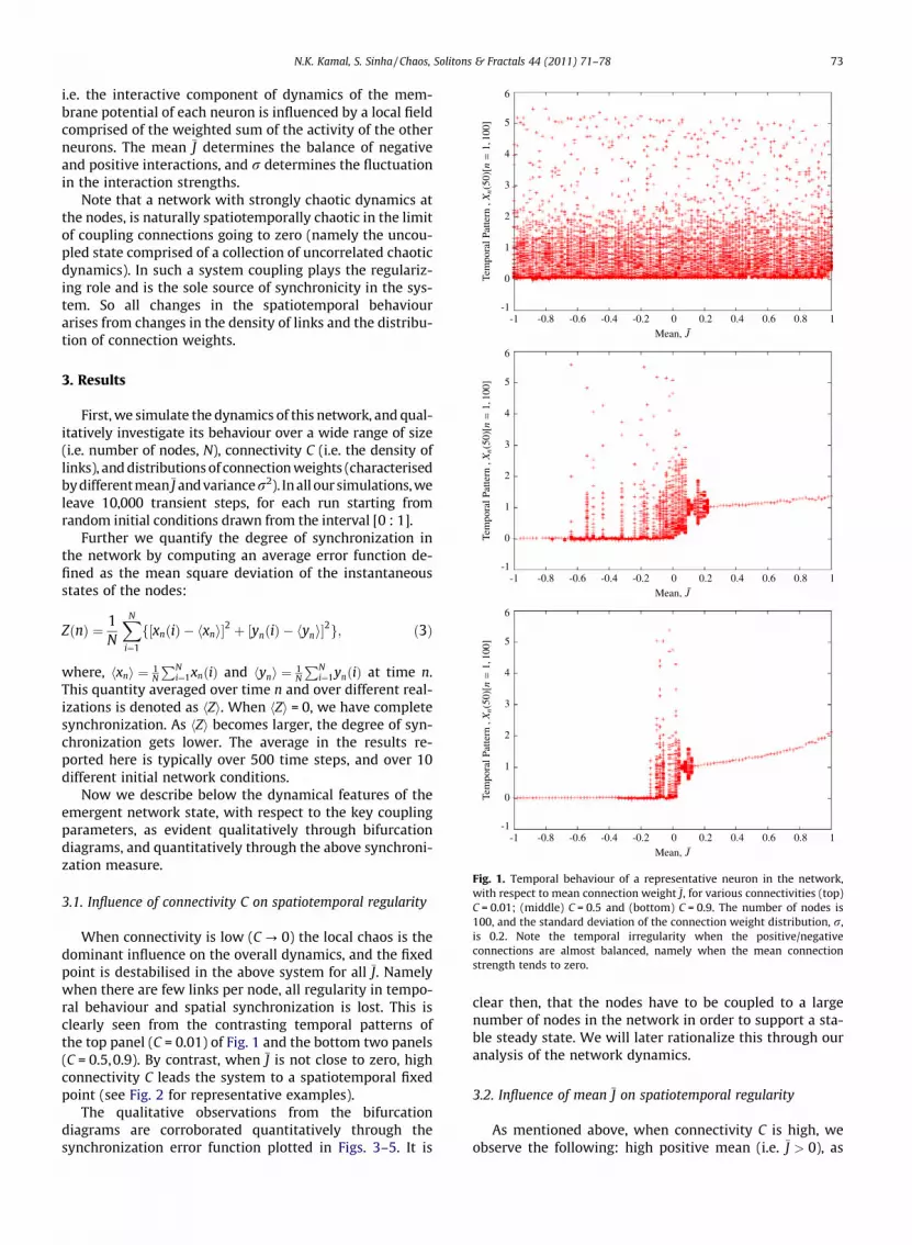
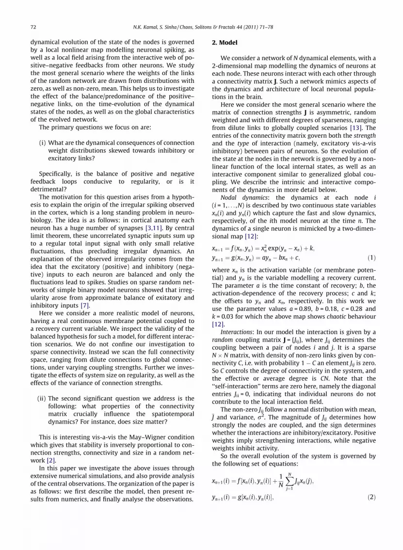
Fig. 1. Temporal behaviour of a representative neuron in the network,with respect to mean connection weight J, for various connectivities (top)C = 0.01; (middle) C = 0.5 and (bottom) C = 0.9. The number of nodes is100, and the standard deviation of the connection weight distribution, r,is 0.2. Note the temporal irregularity when the positive/negativeconnections are almost balanced, namely when the mean connectionstrength tends to zero.

N.K. Kamal, S. Sinha / Chaos, Solitons & Fractals 44 (2011) 71–78 73

i.e. the interactive component of dynamics of the mem-brane potential of each neuron is influenced by a local fieldcomprised of the weighted sum of the activity of the otherneurons. The mean J determines the balance of negativeand positive interactions, and r determines the fluctuationin the interaction strengths.

Note that a network with strongly chaotic dynamics atthe nodes, is naturally spatiotemporally chaotic in the limitof coupling connections going to zero (namely the uncou-pled state comprised of a collection of uncorrelated chaoticdynamics). In such a system coupling plays the regulariz-ing role and is the sole source of synchronicity in the sys-tem. So all changes in the spatiotemporal behaviourarises from changes in the density of links and the distribu-tion of connection weights.

3. Results

First, we simulate the dynamics of this network, and qual-itatively investigate its behaviour over a wide range of size(i.e. number of nodes, N), connectivity C (i.e. the density oflinks), and distributions of connection weights (characterisedby differentmean J and variancer2). In all our simulations, weleave 10,000 transient steps, for each run starting fromrandom initial conditions drawn from the interval [0 : 1].

Further we quantify the degree of synchronization inthe network by computing an average error function de-fined as the mean square deviation of the instantaneousstates of the nodes:

ZðnÞ ¼ 1N

XN

i¼1

f½xnðiÞ � hxni�2 þ ½ynðiÞ � hyni�2g; ð3Þ

where, hxni ¼ 1N

PNi¼1xnðiÞ and hyni ¼ 1

N

PNi¼1ynðiÞ at time n.

This quantity averaged over time n and over different real-izations is denoted as hZi. When hZi = 0, we have completesynchronization. As hZi becomes larger, the degree of syn-chronization gets lower. The average in the results re-ported here is typically over 500 time steps, and over 10different initial network conditions.

Now we describe below the dynamical features of theemergent network state, with respect to the key couplingparameters, as evident qualitatively through bifurcationdiagrams, and quantitatively through the above synchroni-zation measure.

3.1. Influence of connectivity C on spatiotemporal regularity

When connectivity is low (C ? 0) the local chaos is thedominant influence on the overall dynamics, and the fixedpoint is destabilised in the above system for all J. Namelywhen there are few links per node, all regularity in tempo-ral behaviour and spatial synchronization is lost. This isclearly seen from the contrasting temporal patterns ofthe top panel (C = 0.01) of Fig. 1 and the bottom two panels(C = 0.5,0.9). By contrast, when J is not close to zero, highconnectivity C leads the system to a spatiotemporal fixedpoint (see Fig. 2 for representative examples).

The qualitative observations from the bifurcationdiagrams are corroborated quantitatively through thesynchronization error function plotted in Figs. 3–5. It is

clear then, that the nodes have to be coupled to a largenumber of nodes in the network in order to support a sta-ble steady state. We will later rationalize this through ouranalysis of the network dynamics.

3.2. Influence of mean J on spatiotemporal regularity

As mentioned above, when connectivity C is high, weobserve the following: high positive mean (i.e. J > 0), as

0

0.5

1

1.5

2

2.5

3

3.5

0 50 100 150 200

X (n

)

Iteration Step, n

-1

1 0

Fig. 2. Spiking patterns of a representative neuron in a network of sizeN = 100, for mean connection weight J ¼ �1;0;1. Standard deviation, r, ofthe connection weights is 0.2. Note the temporal irregularity of the casewhere the connection weights have zero mean, namely the positive andnegative links are balanced.

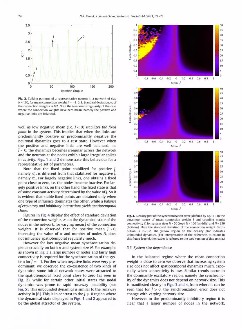
Fig. 3. Density plot of the synchronization error (defined by Eq. (3)) in theparameter space of mean connection weight J and coupling matrixconnectivity C, for system sizes N = 50 (top), N = 100 (middle) and N = 250(bottom). Here the standard deviation of the connection weight distri-bution is r = 0.2. The yellow region on the density plot indicatesunbounded dynamics. (For interpretation of the references to colour inthis figure legend, the reader is referred to the web version of this article.)

74 N.K. Kamal, S. Sinha / Chaos, Solitons & Fractals 44 (2011) 71–78

well as low negative mean (i.e. J < 0) stabilizes the fixedpoint in the system. This implies that when the links arepredominantly positive or predominantly negative theneuronal dynamics goes to a rest state. However whenthe positive and negative links are well balanced, i.e.J � 0, the dynamics becomes irregular across the networkand the neurons at the nodes exhibit large irregular spikesin activity. Figs. 1 and 2 demonstrate this behaviour for arepresentative set of parameters.

Note that the fixed point stabilized for positive J,namely x�þ, is different from that stabilized for negative J,namely x��. For largely negative links, one obtains a fixedpoint close to zero, i.e. the nodes become inactive. For lar-gely positive links, on the other hand, the fixed state is thatof some constant activity determined by the value of J. So itis evident that stable fixed points are obtained only whenone type of influence dominates the other, while a balanceof excitatory and inhibitory interactions yields spatiotemporalchaos.

Figures in Fig. 4 display the effect of standard deviationof the connection weights, r, on the dynamical state of thenodes in the network, for varying mean J of the connectionweights. It is observed that for positive mean J > 0,increasing the value of r and number of nodes N, doesnot influence spatiotemporal regularity much.

However for low negative mean synchronization de-pends crucially on both r and system size N. For example,as shown in Fig. 3 a large number of nodes and fairly highconnectivity is required for the synchronization of the sys-tem for J ¼ �1. Further when negative links were very pre-dominant, we observed the co-existence of two kinds ofdynamics: some initial network states were attracted tothe spatiotemporal fixed point close to zero (as seen inFig. 2), while for certain other initial states the nodaldynamics was prone to rapid runaway instability (seeFig. 5). This unbounded dynamics is similar to the runawayactivity in [6]. This is in contrast to the J P 0 region wherethe dynamical state displayed in Figs. 1 and 2 appeared tobe the global attractor of the system.

3.3. System size dependence

In the balanced regime where the mean connectionweight is close to zero we observe that increasing systemsize does not affect spatiotemporal dynamics much, espe-cially when connectivity is low. Similar trends occur inthe dominantly excitatory region, namely the synchronic-ity of the dynamics does not depend on network size. Thisis manifested clearly in Figs. 3 and 4, from where it can beseen that for J P 0, the synchronization error does notchange with varying network size.

However in the predominantly inhibitory region it isclear that a larger number of nodes in the network,

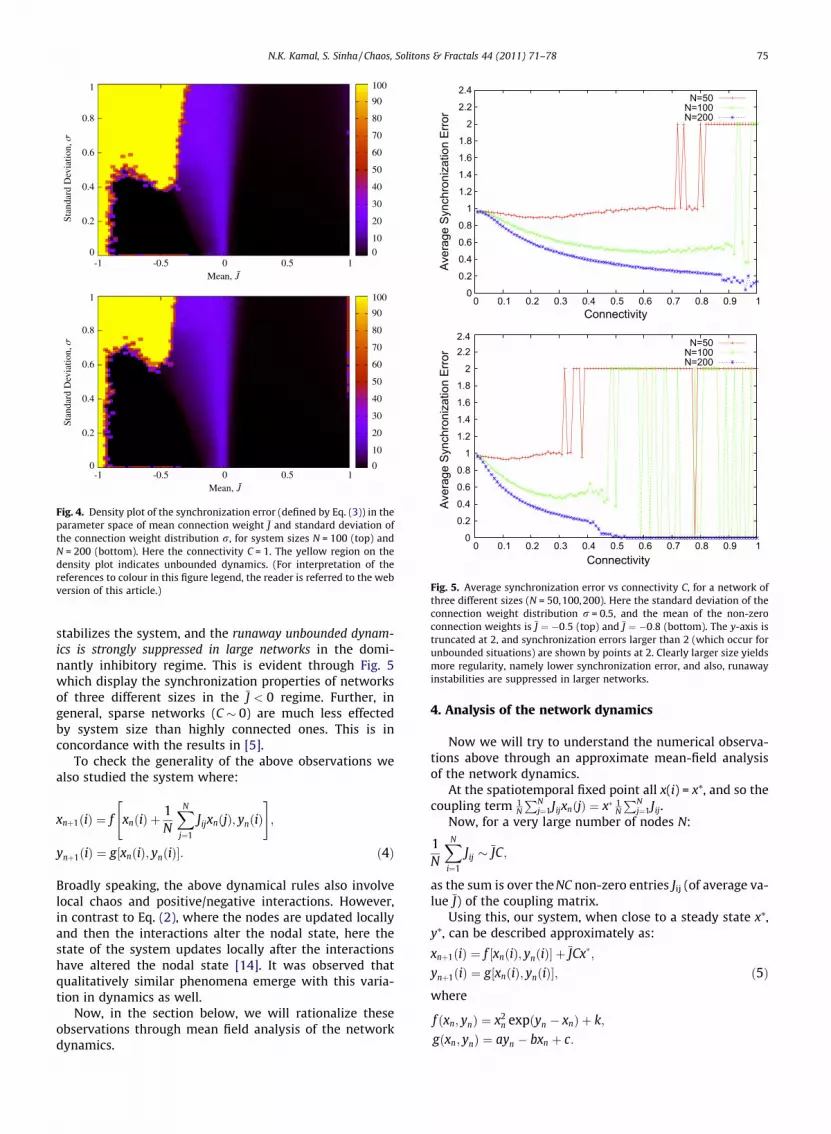
Fig. 4. Density plot of the synchronization error (defined by Eq. (3)) in theparameter space of mean connection weight J and standard deviation ofthe connection weight distribution r, for system sizes N = 100 (top) andN = 200 (bottom). Here the connectivity C = 1. The yellow region on thedensity plot indicates unbounded dynamics. (For interpretation of thereferences to colour in this figure legend, the reader is referred to the webversion of this article.)

0

0.2

0.4

0.6

0.8

1

1.2

1.4

1.6

1.8

2

2.2

2.4

0 0.1 0.2 0.3 0.4 0.5 0.6 0.7 0.8 0.9 1

Aver

age

Sync

hron

izat

ion

Erro

r

Connectivity

N=50N=100N=200

0

0.2

0.4

0.6

0.8

1

1.2

1.4

1.6

1.8

2

2.2 2.4

0 0.1 0.2 0.3 0.4 0.5 0.6 0.7 0.8 0.9 1

Aver

age

Sync

hron

izat

ion

Erro

r

Connectivity

N=50N=100N=200

Fig. 5. Average synchronization error vs connectivity C, for a network ofthree different sizes (N = 50,100,200). Here the standard deviation of theconnection weight distribution r = 0.5, and the mean of the non-zeroconnection weights is J ¼ �0:5 (top) and J ¼ �0:8 (bottom). The y-axis istruncated at 2, and synchronization errors larger than 2 (which occur forunbounded situations) are shown by points at 2. Clearly larger size yieldsmore regularity, namely lower synchronization error, and also, runawayinstabilities are suppressed in larger networks.

N.K. Kamal, S. Sinha / Chaos, Solitons & Fractals 44 (2011) 71–78 75

stabilizes the system, and the runaway unbounded dynam-ics is strongly suppressed in large networks in the domi-nantly inhibitory regime. This is evident through Fig. 5which display the synchronization properties of networksof three different sizes in the J < 0 regime. Further, ingeneral, sparse networks (C � 0) are much less effectedby system size than highly connected ones. This is inconcordance with the results in [5].

To check the generality of the above observations wealso studied the system where:

xnþ1ðiÞ ¼ f xnðiÞ þ1N

XN

j¼1

JijxnðjÞ; ynðiÞ" #

;

ynþ1ðiÞ ¼ g½xnðiÞ; ynðiÞ�: ð4Þ

Broadly speaking, the above dynamical rules also involvelocal chaos and positive/negative interactions. However,in contrast to Eq. (2), where the nodes are updated locallyand then the interactions alter the nodal state, here thestate of the system updates locally after the interactionshave altered the nodal state [14]. It was observed thatqualitatively similar phenomena emerge with this varia-tion in dynamics as well.

Now, in the section below, we will rationalize theseobservations through mean field analysis of the networkdynamics.

4. Analysis of the network dynamics

Now we will try to understand the numerical observa-tions above through an approximate mean-field analysisof the network dynamics.

At the spatiotemporal fixed point all x(i) = x⁄, and so thecoupling term 1

N

PNj¼1JijxnðjÞ ¼ x� 1

N

PNj¼1Jij.

Now, for a very large number of nodes N:

1N

XN

i¼1

Jij � JC;

as the sum is over the NC non-zero entries Jij (of average va-lue J) of the coupling matrix.

Using this, our system, when close to a steady state x⁄,y⁄, can be described approximately as:

xnþ1ðiÞ ¼ f ½xnðiÞ; ynðiÞ� þ JCx�;

ynþ1ðiÞ ¼ g½xnðiÞ; ynðiÞ�; ð5Þwhere

f ðxn; ynÞ ¼ x2n expðyn � xnÞ þ k;

gðxn; ynÞ ¼ ayn � bxn þ c:

76 N.K. Kamal, S. Sinha / Chaos, Solitons & Fractals 44 (2011) 71–78

The approximate evolution equation above is obtained inthe limit of the number of nodes in the system N ?1,and r ? 0. So in order to be closer to this description ofthe network dynamics, the network size has to be largeand the variance of the connection strengths has to besmall.

Now it is immediately clear from Eq. (5) that, in the lim-it C ? 0 (namely extremely sparsely connected neurons)and in the limit J ! 0 (namely when the positive/negativeconnection weights are balanced) one will obtain spatio-temporal chaos. This follows from the fact that both theselimits decouple the neurons, and so the full system be-comes a set of uncoupled, thus uncorrelated, chaotic localneurons. This inference is bourne out by numerics (e.g.Fig. 1).

We will now analyse the stability of spatiotemporalfixed point in Eq. (5), when JC – 0. First, note that the fixedpoint is given as a solution of:

x� ¼ ðx�Þ2 expðy� � x�Þ þ kþ JCx�;

y� ¼ ay� � bx� þ c: ð6Þ

Simplifying the above, by substituting y� ¼ c�bx�

1�a in Eq. (5)we get: randomly selected node of the dynamical

x� ¼ f ðx�Þ ¼ ðx�Þ2 expc � bx�

1� a� x�

� �þ kþ JCx�: ð7Þ

We use the above effective equation, which reduces the Ncoupled chaotic neuronal maps to an effective dynamicalmap describing one neuron in a mean field of couplinginteractions, as the starting point of our stability analysis.That is, the dynamics of any particular node of the networkis similar to the dynamics of a single neuron with an effec-tive k value approximately equal to kþ JCx�. This immedi-ately also gives that when J � 0, or when C � 0, the

-3

-2

-1

0

1

2

3

4

5

0 0.5 1 1

f(x)

-0.2 0

0.2 0.4 0.6 0.8

1 1.2

0 0.2 0.4

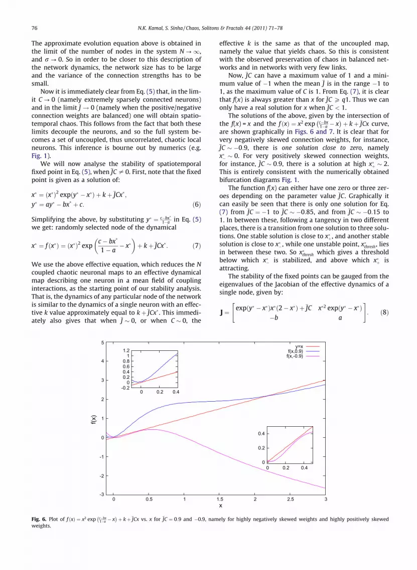
Fig. 6. Plot of f ðxÞ ¼ x2 exp c�bx1�a � x� �

þ kþ JCx vs. x for JC ¼ 0:9 and �0.9, namweights.

effective k is the same as that of the uncoupled map,namely the value that yields chaos. So this is consistentwith the observed preservation of chaos in balanced net-works and in networks with very few links.

Now, JC can have a maximum value of 1 and a mini-mum value of �1 when the mean J is in the range �1 to1, as the maximum value of C is 1. From Eq. (7), it is clearthat f(x) is always greater than x for JC P q1. Thus we canonly have a real solution for x when JC < 1.

The solutions of the above, given by the intersection ofthe f(x) = x and the f ðxÞ ¼ x2 exp c�bx

1�a � x� �

þ kþ JCx curve,are shown graphically in Figs. 6 and 7. It is clear that forvery negatively skewed connection weights, for instance,JC � �0:9, there is one solution close to zero, namelyx�� � 0. For very positively skewed connection weights,for instance, JC � 0:9, there is a solution at high x�þ � 2.This is entirely consistent with the numerically obtainedbifurcation diagrams Fig. 1.

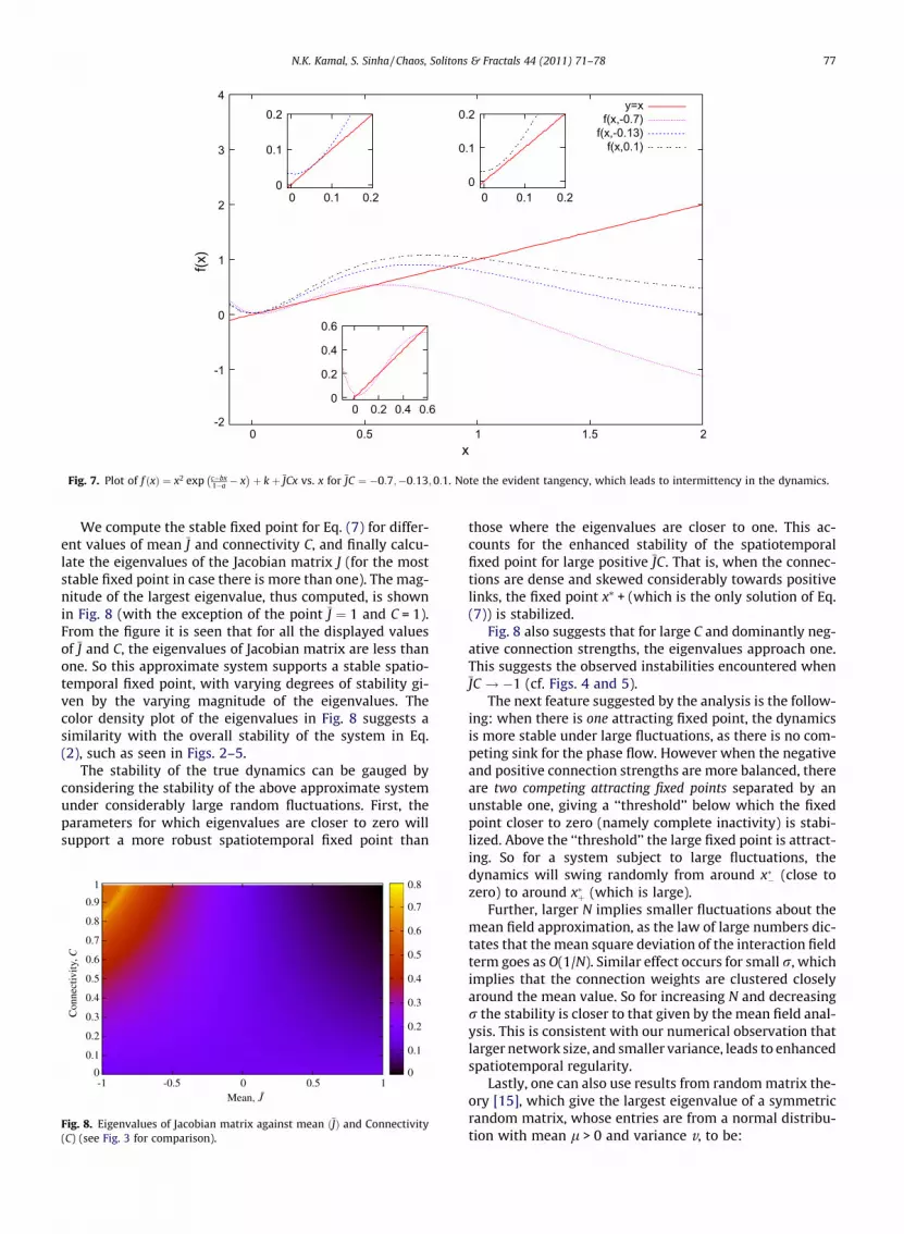
The function f(x) can either have one zero or three zer-oes depending on the parameter value JC. Graphically itcan easily be seen that there is only one solution for Eq.(7) from JC ¼ �1 to JC � �0:85, and from JC � �0:15 to1. In between these, following a tangency in two differentplaces, there is a transition from one solution to three solu-tions. One stable solution is close to x�þ, and another stablesolution is close to x��, while one unstable point, x�thresh, liesin between these two. So x�thresh which gives a thresholdbelow which x�� is stabilized, and above which x�þ isattracting.

The stability of the fixed points can be gauged from theeigenvalues of the Jacobian of the effective dynamics of asingle node, given by:

J ¼ expðy� � x�Þx�ð2� x�Þ þ JC x�2 expðy� � x�Þ�b a

" #: ð8Þ

.5 2 2.5 3x

y=xf(x,0.9)

f(x,-0.9)

0

0.2

0.4

0 0.2 0.4

ely for highly negatively skewed weights and highly positively skewed

-2

-1

0

1

2

3

4

0 0.5 1 1.5 2

f(x)

x

y=xf(x,-0.7)

f(x,-0.13)f(x,0.1)

0

0.1

0.2

0 0.1 0.2

0

0.2

0.4

0.6

0 0.2 0.4 0.6

0

0.1

0.2

0 0.1 0.2

Fig. 7. Plot of f ðxÞ ¼ x2 exp c�bx1�a � x� �

þ kþ JCx vs. x for JC ¼ �0:7;�0:13;0:1. Note the evident tangency, which leads to intermittency in the dynamics.

N.K. Kamal, S. Sinha / Chaos, Solitons & Fractals 44 (2011) 71–78 77

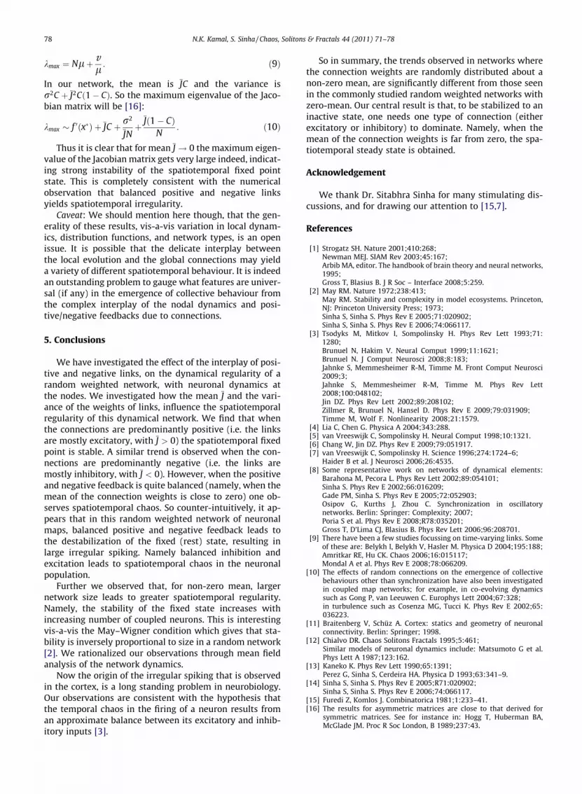
We compute the stable fixed point for Eq. (7) for differ-ent values of mean J and connectivity C, and finally calcu-late the eigenvalues of the Jacobian matrix J (for the moststable fixed point in case there is more than one). The mag-nitude of the largest eigenvalue, thus computed, is shownin Fig. 8 (with the exception of the point J ¼ 1 and C = 1).From the figure it is seen that for all the displayed valuesof J and C, the eigenvalues of Jacobian matrix are less thanone. So this approximate system supports a stable spatio-temporal fixed point, with varying degrees of stability gi-ven by the varying magnitude of the eigenvalues. Thecolor density plot of the eigenvalues in Fig. 8 suggests asimilarity with the overall stability of the system in Eq.(2), such as seen in Figs. 2–5.

The stability of the true dynamics can be gauged byconsidering the stability of the above approximate systemunder considerably large random fluctuations. First, theparameters for which eigenvalues are closer to zero willsupport a more robust spatiotemporal fixed point than

Fig. 8. Eigenvalues of Jacobian matrix against mean ðJÞ and Connectivity(C) (see Fig. 3 for comparison).

those where the eigenvalues are closer to one. This ac-counts for the enhanced stability of the spatiotemporalfixed point for large positive JC. That is, when the connec-tions are dense and skewed considerably towards positivelinks, the fixed point x⁄ + (which is the only solution of Eq.(7)) is stabilized.

Fig. 8 also suggests that for large C and dominantly neg-ative connection strengths, the eigenvalues approach one.This suggests the observed instabilities encountered whenJC ! �1 (cf. Figs. 4 and 5).

The next feature suggested by the analysis is the follow-ing: when there is one attracting fixed point, the dynamicsis more stable under large fluctuations, as there is no com-peting sink for the phase flow. However when the negativeand positive connection strengths are more balanced, thereare two competing attracting fixed points separated by anunstable one, giving a ‘‘threshold’’ below which the fixedpoint closer to zero (namely complete inactivity) is stabi-lized. Above the ‘‘threshold’’ the large fixed point is attract-ing. So for a system subject to large fluctuations, thedynamics will swing randomly from around x�� (close tozero) to around x�þ (which is large).

Further, larger N implies smaller fluctuations about themean field approximation, as the law of large numbers dic-tates that the mean square deviation of the interaction fieldterm goes as O(1/N). Similar effect occurs for small r, whichimplies that the connection weights are clustered closelyaround the mean value. So for increasing N and decreasingr the stability is closer to that given by the mean field anal-ysis. This is consistent with our numerical observation thatlarger network size, and smaller variance, leads to enhancedspatiotemporal regularity.

Lastly, one can also use results from random matrix the-ory [15], which give the largest eigenvalue of a symmetricrandom matrix, whose entries are from a normal distribu-tion with mean l > 0 and variance v, to be:

78 N.K. Kamal, S. Sinha / Chaos, Solitons & Fractals 44 (2011) 71–78

kmax ¼ Nlþ vl: ð9Þ

In our network, the mean is JC and the variance isr2C þ J2Cð1� CÞ. So the maximum eigenvalue of the Jaco-bian matrix will be [16]:

kmax � f 0ðx�Þ þ JC þ r2

JNþ Jð1� CÞ

N: ð10Þ

Thus it is clear that for mean J ! 0 the maximum eigen-value of the Jacobian matrix gets very large indeed, indicat-ing strong instability of the spatiotemporal fixed pointstate. This is completely consistent with the numericalobservation that balanced positive and negative linksyields spatiotemporal irregularity.

Caveat: We should mention here though, that the gen-erality of these results, vis-a-vis variation in local dynam-ics, distribution functions, and network types, is an openissue. It is possible that the delicate interplay betweenthe local evolution and the global connections may yielda variety of different spatiotemporal behaviour. It is indeedan outstanding problem to gauge what features are univer-sal (if any) in the emergence of collective behaviour fromthe complex interplay of the nodal dynamics and posi-tive/negative feedbacks due to connections.

5. Conclusions

We have investigated the effect of the interplay of posi-tive and negative links, on the dynamical regularity of arandom weighted network, with neuronal dynamics atthe nodes. We investigated how the mean J and the vari-ance of the weights of links, influence the spatiotemporalregularity of this dynamical network. We find that whenthe connections are predominantly positive (i.e. the linksare mostly excitatory, with J > 0) the spatiotemporal fixedpoint is stable. A similar trend is observed when the con-nections are predominantly negative (i.e. the links aremostly inhibitory, with J < 0). However, when the positiveand negative feedback is quite balanced (namely, when themean of the connection weights is close to zero) one ob-serves spatiotemporal chaos. So counter-intuitively, it ap-pears that in this random weighted network of neuronalmaps, balanced positive and negative feedback leads tothe destabilization of the fixed (rest) state, resulting inlarge irregular spiking. Namely balanced inhibition andexcitation leads to spatiotemporal chaos in the neuronalpopulation.

Further we observed that, for non-zero mean, largernetwork size leads to greater spatiotemporal regularity.Namely, the stability of the fixed state increases withincreasing number of coupled neurons. This is interestingvis-a-vis the May–Wigner condition which gives that sta-bility is inversely proportional to size in a random network[2]. We rationalized our observations through mean fieldanalysis of the network dynamics.

Now the origin of the irregular spiking that is observedin the cortex, is a long standing problem in neurobiology.Our observations are consistent with the hypothesis thatthe temporal chaos in the firing of a neuron results froman approximate balance between its excitatory and inhib-itory inputs [3].

So in summary, the trends observed in networks wherethe connection weights are randomly distributed about anon-zero mean, are significantly different from those seenin the commonly studied random weighted networks withzero-mean. Our central result is that, to be stabilized to aninactive state, one needs one type of connection (eitherexcitatory or inhibitory) to dominate. Namely, when themean of the connection weights is far from zero, the spa-tiotemporal steady state is obtained.

Acknowledgement

We thank Dr. Sitabhra Sinha for many stimulating dis-cussions, and for drawing our attention to [15,7].

References

[1] Strogatz SH. Nature 2001;410:268;Newman MEJ. SIAM Rev 2003;45:167;Arbib MA, editor. The handbook of brain theory and neural networks,1995;Gross T, Blasius B. J R Soc – Interface 2008;5:259.

[2] May RM. Nature 1972;238:413;May RM. Stability and complexity in model ecosystems. Princeton,NJ: Princeton University Press; 1973;Sinha S, Sinha S. Phys Rev E 2005;71:020902;Sinha S, Sinha S. Phys Rev E 2006;74:066117.

[3] Tsodyks M, Mitkov I, Sompolinsky H. Phys Rev Lett 1993;71:1280;Brunuel N, Hakim V. Neural Comput 1999;11:1621;Brunuel N. J Comput Neurosci 2008;8:183;Jahnke S, Memmesheimer R-M, Timme M. Front Comput Neurosci2009;3;Jahnke S, Memmesheimer R-M, Timme M. Phys Rev Lett2008;100:048102;Jin DZ. Phys Rev Lett 2002;89:208102;Zillmer R, Brunuel N, Hansel D. Phys Rev E 2009;79:031909;Timme M, Wolf F. Nonlinearity 2008;21:1579.

[4] Lia C, Chen G. Physica A 2004;343:288.[5] van Vreeswijk C, Sompolinsky H. Neural Comput 1998;10:1321.[6] Chang W, Jin DZ. Phys Rev E 2009;79:051917.[7] van Vreeswijk C, Sompolinsky H. Science 1996;274:1724–6;

Haider B et al. J Neurosci 2006;26:4535.[8] Some representative work on networks of dynamical elements:

Barahona M, Pecora L. Phys Rev Lett 2002;89:054101;Sinha S. Phys Rev E 2002;66:016209;Gade PM, Sinha S. Phys Rev E 2005;72:052903;Osipov G, Kurths J, Zhou C. Synchronization in oscillatorynetworks. Berlin: Springer: Complexity; 2007;Poria S et al. Phys Rev E 2008;R78:035201;Gross T, D’Lima CJ, Blasius B. Phys Rev Lett 2006;96:208701.

[9] There have been a few studies focussing on time-varying links. Someof these are: Belykh I, Belykh V, Hasler M. Physica D 2004;195:188;Amritkar RE, Hu CK. Chaos 2006;16:015117;Mondal A et al. Phys Rev E 2008;78:066209.

[10] The effects of random connections on the emergence of collectivebehaviours other than synchronization have also been investigatedin coupled map networks; for example, in co-evolving dynamicssuch as Gong P, van Leeuwen C. Europhys Lett 2004;67:328;in turbulence such as Cosenza MG, Tucci K. Phys Rev E 2002;65:036223.

[11] Braitenberg V, Schüz A. Cortex: statics and geometry of neuronalconnectivity. Berlin: Springer; 1998.

[12] Chialvo DR. Chaos Solitons Fractals 1995;5:461;Similar models of neuronal dynamics include: Matsumoto G et al.Phys Lett A 1987;123:162.

[13] Kaneko K. Phys Rev Lett 1990;65:1391;Perez G, Sinha S, Cerdeira HA. Physica D 1993;63:341–9.

[14] Sinha S, Sinha S. Phys Rev E 2005;R71:020902;Sinha S, Sinha S. Phys Rev E 2006;74:066117.

[15] Furedi Z, Komlos J. Combinatorica 1981;1:233–41.[16] The results for asymmetric matrices are close to that derived for

symmetric matrices. See for instance in: Hogg T, Huberman BA,McGlade JM. Proc R Soc London, B 1989;237:43.