ifs documentation part vi: technical and - ecmwf
TRANSCRIPT
IFS Documentation Cycle CY25r1
F
IFS DOCUMENTATION
PART VI: T ECHNICAL AND
COMPUTATIONAL PROCEDURES (CY25R1)(Operational implementation 9 April 2002)
Edited by Peter W. White
(Text written and updated by members of Météo-France and the ECMWResearch Department)
Table of contents
Chapter 1. Technical overview
Chapter 2. FULL-POS post-processing and interpolation
Chapter 3. Parallel implementation
REFERENCES
1
IFS Documentationn Cycle CY25r1 (Edited 2003)
Part VI: ‘Technical and computational procedures (CY25R1)’
e Eu-
her than
in this
ecasts
Copyright
© ECMWF, 2003.
All information, text, and electronic images contained within this document are the intellectual property of th
ropean Centre for Medium-Range Weather Forecasts and may not be reproduced or used in any way (ot
for personal use) without permission. Any user of any information, text, or electronic images contained with
document accepts all responsibility for the use. In particular, no claims of accuracy or precision of the for
will be made which is inappropriate to their scientific basis.
2
IFS Documentation Cycle CY25r1 (Edited 2003)
IFS Documentation Cycle CY25r1
w the
ctions:
Part VI: T ECHNICAL AND COMPUTATIONAL PROCEDURES
CHAPTER 1 Technical overview
Table of contents
1.1 Introduction
1.2 Configurations
1.3 Configuration control
1.4 Initial data
1.4.1 Forecast model, NCONF=1
1.5 Command line option
1.6 Namelist control
1.6.1 Index of Namelists
1.7 Post processing
1.8 Restart capability
1.9 Mass conservation
1.1 INTRODUCTION
This chapter describes the high level technical structure of IFS, how it can be supplied with initial data, ho
execution is controlled, and how output fields can be generated. The chapter is divided into the following se
1) Configurations
2) Initial data
3) Command line options
4) Namelist control
5) Post processing
6) Restart capability
7) Mass conservation
1
IFS Documentationn Cycle CY25r1 (Edited 2003)
Part VI: ‘Technical and computational procedures’
cution
y
amelist
indi-
es.
1.2 CONFIGURATIONS
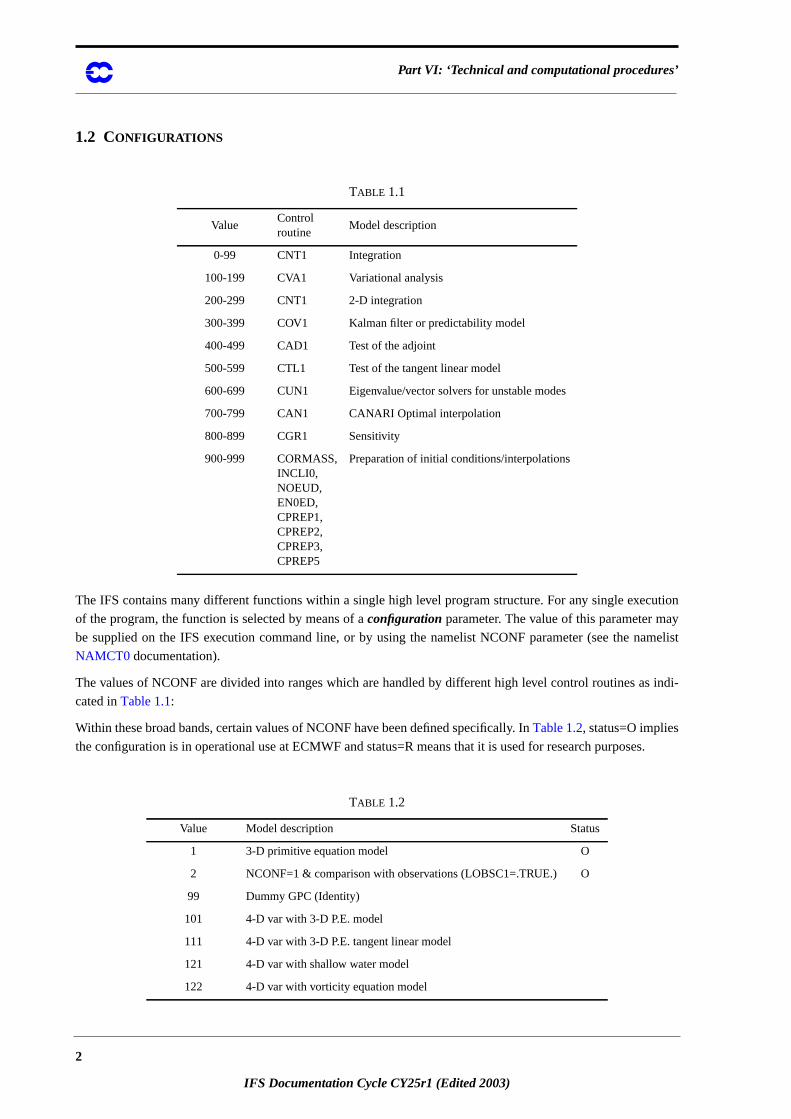
The IFS contains many different functions within a single high level program structure. For any single exe
of the program, the function is selected by means of aconfiguration parameter. The value of this parameter ma
be supplied on the IFS execution command line, or by using the namelist NCONF parameter (see the n
NAMCT0 documentation).
The values of NCONF are divided into ranges which are handled by different high level control routines as
cated inTable 1.1:
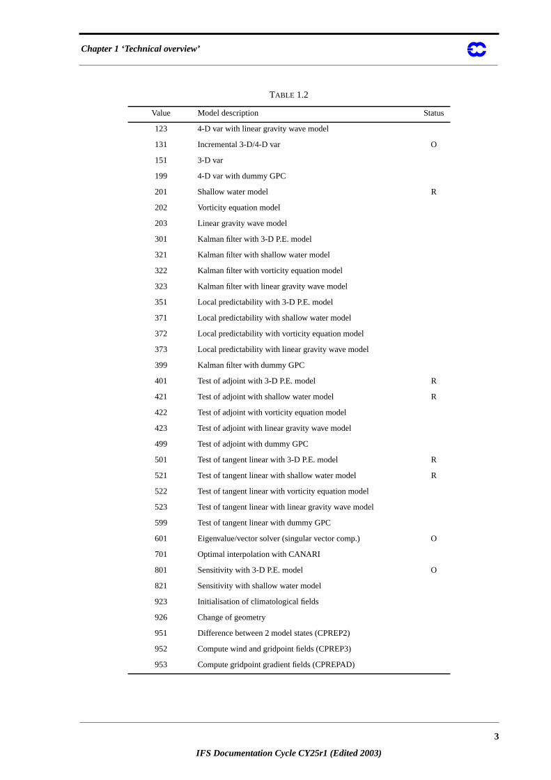
Within these broad bands, certain values of NCONF have been defined specifically. InTable 1.2, status=O implies
the configuration is in operational use at ECMWF and status=R means that it is used for research purpos
TABLE 1.1
ValueControlroutine
Model description
0-99 CNT1 Integration
100-199 CVA1 Variational analysis
200-299 CNT1 2-D integration
300-399 COV1 Kalman filter or predictability model
400-499 CAD1 Test of the adjoint
500-599 CTL1 Test of the tangent linear model
600-699 CUN1 Eigenvalue/vector solvers for unstable modes
700-799 CAN1 CANARI Optimal interpolation
800-899 CGR1 Sensitivity
900-999 CORMASS,INCLI0,NOEUD,EN0ED,CPREP1,CPREP2,CPREP3,CPREP5
Preparation of initial conditions/interpolations
TABLE 1.2
Value Model description Status
1 3-D primitive equation model O
2 NCONF=1 & comparison with observations (LOBSC1=.TRUE.) O
99 Dummy GPC (Identity)
101 4-D var with 3-D P.E. model
111 4-D var with 3-D P.E. tangent linear model
121 4-D var with shallow water model
122 4-D var with vorticity equation model
2
IFS Documentation Cycle CY25r1 (Edited 2003)
Chapter 1 ‘Technical overview’
123 4-D var with linear gravity wave model
131 Incremental 3-D/4-D var O
151 3-D var
199 4-D var with dummy GPC
201 Shallow water model R
202 Vorticity equation model
203 Linear gravity wave model
301 Kalman filter with 3-D P.E. model
321 Kalman filter with shallow water model
322 Kalman filter with vorticity equation model
323 Kalman filter with linear gravity wave model
351 Local predictability with 3-D P.E. model
371 Local predictability with shallow water model
372 Local predictability with vorticity equation model
373 Local predictability with linear gravity wave model
399 Kalman filter with dummy GPC
401 Test of adjoint with 3-D P.E. model R
421 Test of adjoint with shallow water model R
422 Test of adjoint with vorticity equation model
423 Test of adjoint with linear gravity wave model
499 Test of adjoint with dummy GPC
501 Test of tangent linear with 3-D P.E. model R
521 Test of tangent linear with shallow water model R
522 Test of tangent linear with vorticity equation model
523 Test of tangent linear with linear gravity wave model
599 Test of tangent linear with dummy GPC
601 Eigenvalue/vector solver (singular vector comp.) O
701 Optimal interpolation with CANARI
801 Sensitivity with 3-D P.E. model O
821 Sensitivity with shallow water model
923 Initialisation of climatological fields
926 Change of geometry
951 Difference between 2 model states (CPREP2)
952 Compute wind and gridpoint fields (CPREP3)
953 Compute gridpoint gradient fields (CPREPAD)
TABLE 1.2
Value Model description Status
3
IFS Documentation Cycle CY25r1 (Edited 2003)
Part VI: ‘Technical and computational procedures’
for
er var-
means
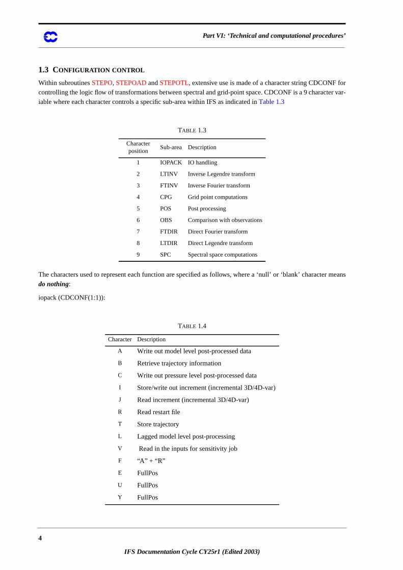
1.3 CONFIGURATION CONTROL
Within subroutinesSTEPO, STEPOADandSTEPOTL, extensive use is made of a character string CDCONF
controlling the logic flow of transformations between spectral and grid-point space. CDCONF is a 9 charact
iable where each character controls a specific sub-area within IFS as indicated inTable 1.3
The characters used to represent each function are specified as follows, where a ‘null’ or ‘blank’ character
do nothing:
iopack (CDCONF(1:1)):
TABLE 1.3
Characterposition
Sub-area Description
1 IOPACK IO handling
2 LTINV Inverse Legendre transform
3 FTINV Inverse Fourier transform
4 CPG Grid point computations
5 POS Post processing
6 OBS Comparison with observations
7 FTDIR Direct Fourier transform
8 LTDIR Direct Legendre transform
9 SPC Spectral space computations
TABLE 1.4
Character Description
A Write out model level post-processed data
B Retrieve trajectory information
C Write out pressure level post-processed data
I Store/write out increment (incremental 3D/4D-var)
J Read increment (incremental 3D/4D-var)
R Read restart file
T Store trajectory
L Lagged model level post-processing
V Read in the inputs for sensitivity job
F “A” + “R”
E FullPos
U FullPos
Y FullPos
4
IFS Documentation Cycle CY25r1 (Edited 2003)
Chapter 1 ‘Technical overview’
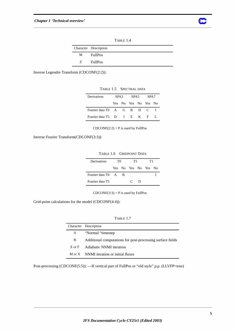
Inverse Legendre Transform (CDCONF(2:2)):
CDCONF(2:2) = P is used by FullPos
Inverse Fourier Transform(CDCONF(3:3)):
CDCONF(3:3) = P is used by FullPos
Grid-point calculations for the model (CDCONF(4:4)):
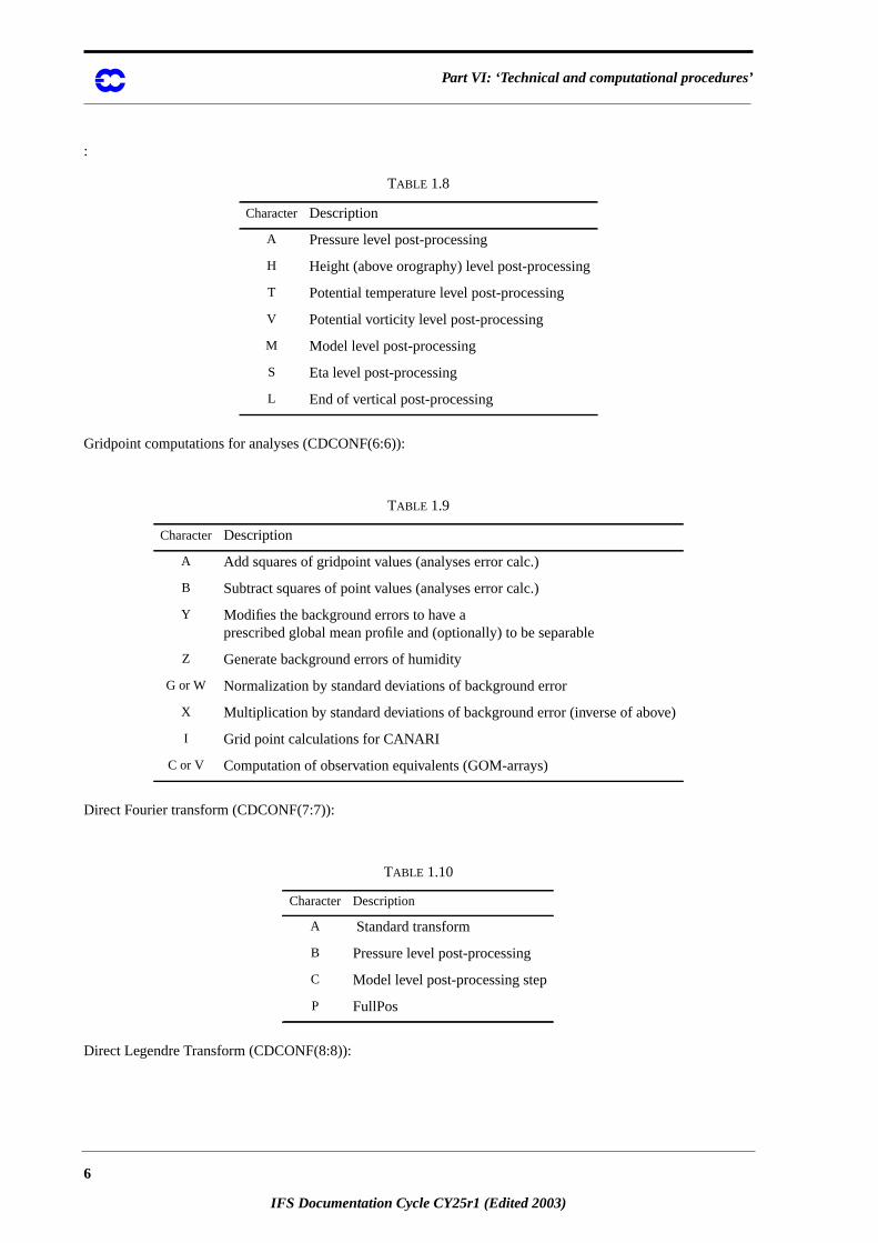
Post-processing (CDCONF(5:5)): —If vertical part of FullPos or “old style” p.p. (LLVFP=true)
M FullPos
Z FullPos
TABLE 1.5 SPECTRAL DATA
Derivatives SPA3 SPA5 SPA7
Yes No Yes No Yes No
Fourier data T0 A G B H C I
Fourier data T5 D J E K F L
TABLE 1.6 GRIDPOINT DATA
Derivatives T0 T5 T1
Yes No Yes No Yes No
Fourier data T0 A B I
Fourier data T5 C D
TABLE 1.7
Character Description
A “Normal “timestep
B Additional computations for post-processing surface fields
E or F Adiabatic NNMI iteration
M or X NNMI iteration or initial fluxes
TABLE 1.4
Character Description
5
IFS Documentation Cycle CY25r1 (Edited 2003)
Part VI: ‘Technical and computational procedures’
:
Gridpoint computations for analyses (CDCONF(6:6)):
Direct Fourier transform (CDCONF(7:7)):
Direct Legendre Transform (CDCONF(8:8)):
TABLE 1.8
Character Description
A Pressure level post-processing
H Height (above orography) level post-processing
T Potential temperature level post-processing
V Potential vorticity level post-processing
M Model level post-processing
S Eta level post-processing
L End of vertical post-processing
TABLE 1.9
Character Description
A Add squares of gridpoint values (analyses error calc.)
B Subtract squares of point values (analyses error calc.)
Y Modifies the background errors to have aprescribed global mean profile and (optionally) to be separable
Z Generate background errors of humidity
G or W Normalization by standard deviations of background error
X Multiplication by standard deviations of background error (inverse of above)
I Grid point calculations for CANARI
C or V Computation of observation equivalents (GOM-arrays)
TABLE 1.10
Character Description
A Standard transform
B Pressure level post-processing
C Model level post-processing step
P FullPos
6
IFS Documentation Cycle CY25r1 (Edited 2003)
Chapter 1 ‘Technical overview’
. The
scrip-
d file
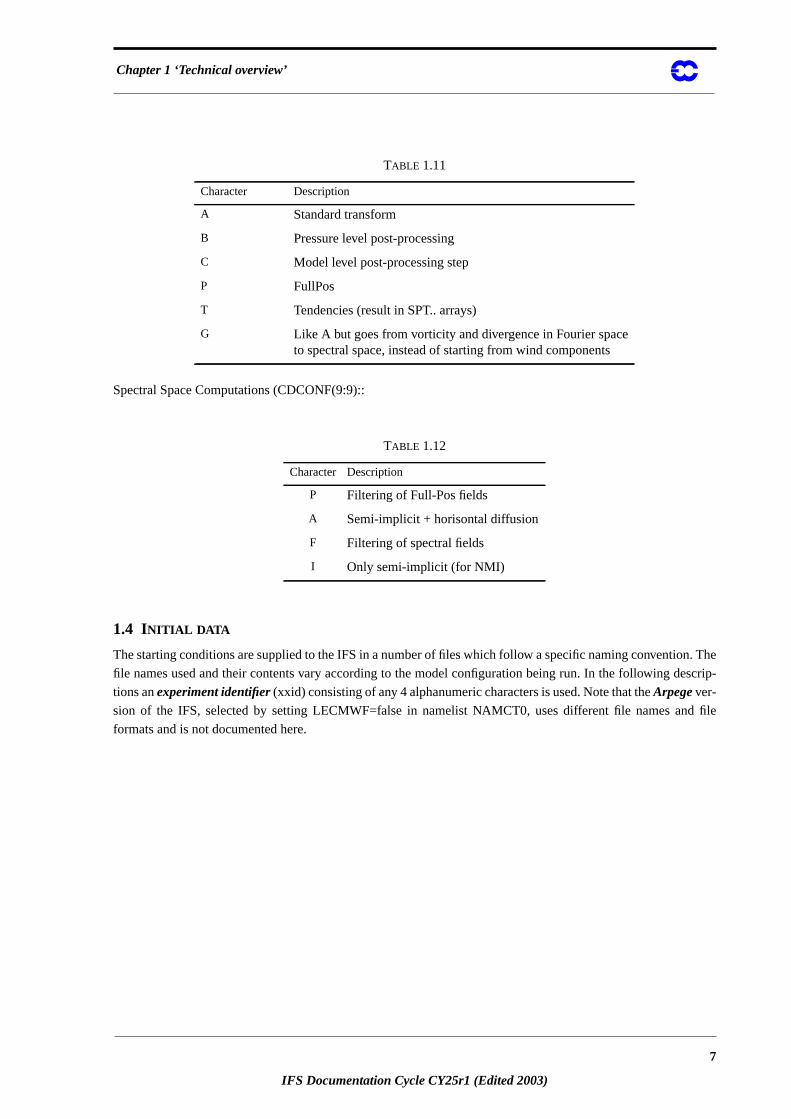
Spectral Space Computations (CDCONF(9:9)::
1.4 INITIAL DATA
The starting conditions are supplied to the IFS in a number of files which follow a specific naming convention
file names used and their contents vary according to the model configuration being run. In the following de
tions anexperiment identifier(xxid) consisting of any 4 alphanumeric characters is used. Note that theArpegever-
sion of the IFS, selected by setting LECMWF=false in namelist NAMCT0, uses different file names an
formats and is not documented here.
TABLE 1.11
Character Description
A Standard transform
B Pressure level post-processing
C Model level post-processing step
P FullPos
T Tendencies (result in SPT.. arrays)
G Like A but goes from vorticity and divergence in Fourier spaceto spectral space, instead of starting from wind components
TABLE 1.12
Character Description
P Filtering of Full-Pos fields
A Semi-implicit + horisontal diffusion
F Filtering of spectral fields
I Only semi-implicit (for NMI)
7
IFS Documentation Cycle CY25r1 (Edited 2003)
Part VI: ‘Technical and computational procedures’
nd
d,
which
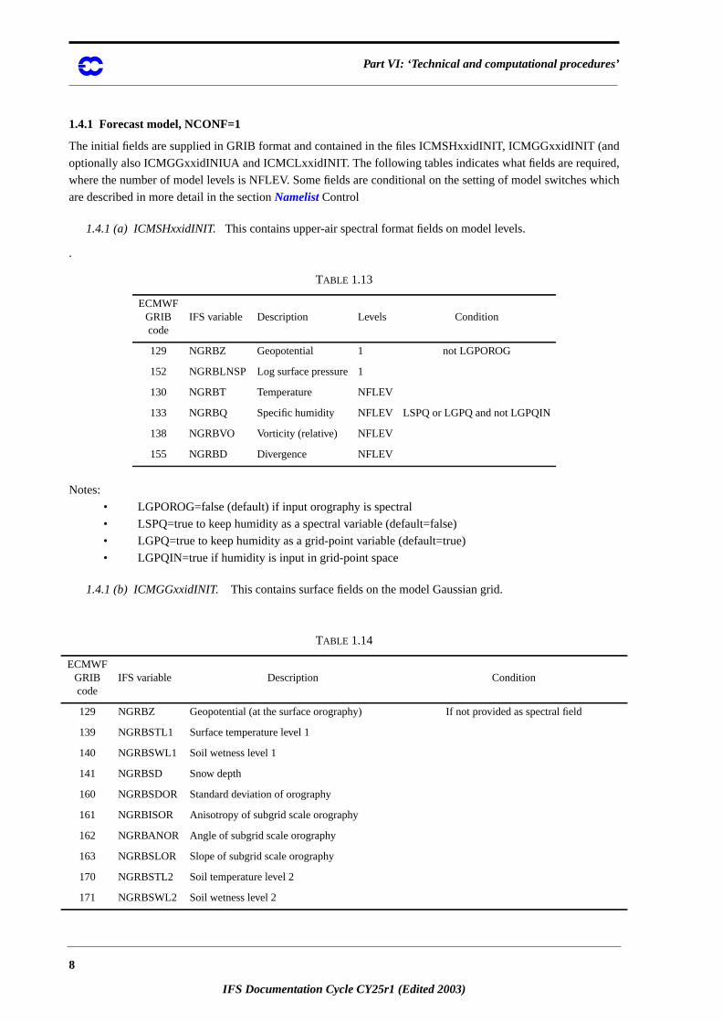
1.4.1 Forecast model, NCONF=1
The initial fields are supplied in GRIB format and contained in the files ICMSHxxidINIT, ICMGGxxidINIT (a
optionally also ICMGGxxidINIUA and ICMCLxxidINIT. The following tables indicates what fields are require
where the number of model levels is NFLEV. Some fields are conditional on the setting of model switches
are described in more detail in the sectionNamelistControl
1.4.1 (a) ICMSHxxidINIT.This contains upper-air spectral format fields on model levels.
.
Notes:
• LGPOROG=false (default) if input orography is spectral
• LSPQ=true to keep humidity as a spectral variable (default=false)
• LGPQ=true to keep humidity as a grid-point variable (default=true)
• LGPQIN=true if humidity is input in grid-point space
1.4.1 (b) ICMGGxxidINIT. This contains surface fields on the model Gaussian grid.
TABLE 1.13
ECMWFGRIBcode
IFS variable Description Levels Condition
129 NGRBZ Geopotential 1 not LGPOROG
152 NGRBLNSP Log surface pressure 1
130 NGRBT Temperature NFLEV
133 NGRBQ Specific humidity NFLEV LSPQ or LGPQ and not LGPQIN
138 NGRBVO Vorticity (relative) NFLEV
155 NGRBD Divergence NFLEV
TABLE 1.14
ECMWFGRIBcode
IFS variable Description Condition
129 NGRBZ Geopotential (at the surface orography) If not provided as spectral field
139 NGRBSTL1 Surface temperature level 1
140 NGRBSWL1 Soil wetness level 1
141 NGRBSD Snow depth
160 NGRBSDOR Standard deviation of orography
161 NGRBISOR Anisotropy of subgrid scale orography
162 NGRBANOR Angle of subgrid scale orography
163 NGRBSLOR Slope of subgrid scale orography
170 NGRBSTL2 Soil temperature level 2
171 NGRBSWL2 Soil wetness level 2
8
IFS Documentation Cycle CY25r1 (Edited 2003)
Chapter 1 ‘Technical overview’
ero
h inte-
assim-
values
del)
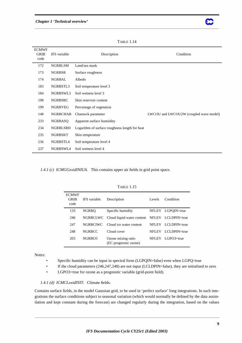
1.4.1 (c) ICMGGxxidINIUA.This contains upper air fields in grid point space.
Notes:
• Specific humidity can be input in spectral form (LGPQIN=false) even when LGPQ=true
• If the cloud parameters (246,247,248) are not input (LCLDPIN=false), they are initialised to z
• LGPO3=true for ozone as a prognostic variable (grid-point field).
1.4.1 (d) ICMCLxxidINIT. Climate fields.
Contains surface fields, in the model Gaussian grid, to be used in ‘perfect surface’ long integrations. In suc
grations the surface conditions subject to seasonal variation (which would normally be defined by the data
ilation and kept constant during the forecast) are changed regularly during the integration, based on the
172 NGRBLSM Land/sea mask
173 NGRBSR Surface roughness
174 NGRBAL Albedo
183 NGRBSTL3 Soil temperature level 3
184 NGRBSWL3 Soil wetness level 3
198 NGRBSRC Skin reservoir content
199 NGRBVEG Percentage of vegetation
148 NGRBCHAR Charnock parameter LWCOU and LWCOU2W (coupled wave mo
233 NGRBASQ Apparent surface humiidity
234 NGRBLSRH Logarithm of surface roughness length for heat
235 NGRBSKT Skin temperature
236 NGRBSTL4 Soil temperature level 4
237 NGRBSWL4 Soil wetness level 4
TABLE 1.15
ECMWFGRIBcode
IFS variable Description Levels Condition
133 NGRBQ Specific humidity NFLEV LGPQIN=true
246 NGRBCLWC Cloud liquid water content NFLEV LCLDPIN=true
247 NGRBCIWC Cloud ice water content NFLEV LCLDPIN=true
248 NGRBCC Cloud cover NFLEV LCLDPIN=true
203 NGRBO3 Ozone mixing ratio(EC prognostic ozone)
NFLEV LGPO3=true
TABLE 1.14
ECMWFGRIBcode
IFS variable Description Condition
9
IFS Documentation Cycle CY25r1 (Edited 2003)
Part VI: ‘Technical and computational procedures’
uld be
tion pe-
e
his is
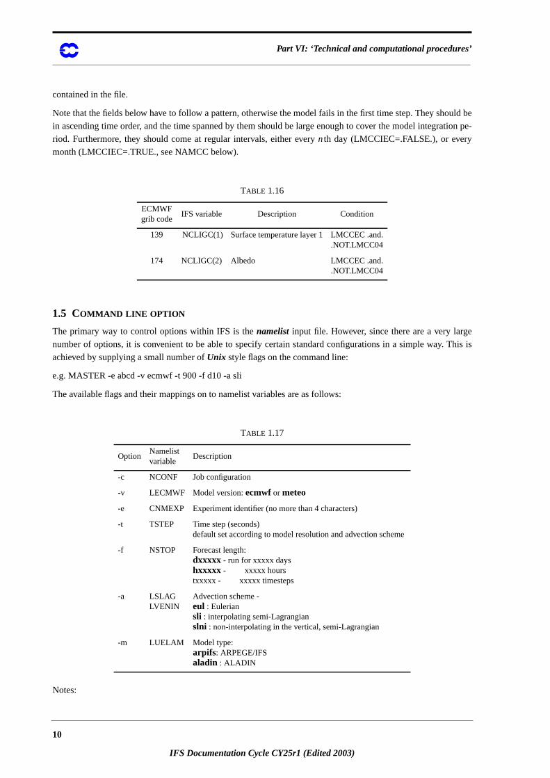
contained in the file.
Note that the fields below have to follow a pattern, otherwise the model fails in the first time step. They sho
in ascending time order, and the time spanned by them should be large enough to cover the model integra
riod. Furthermore, they should come at regular intervals, either everynth day (LMCCIEC=.FALSE.), or every
month (LMCCIEC=.TRUE., see NAMCC below).
1.5 COMMAND LINE OPTION
The primary way to control options within IFS is thenamelist input file. However, since there are a very larg
number of options, it is convenient to be able to specify certain standard configurations in a simple way. T
achieved by supplying a small number ofUnix style flags on the command line:
e.g. MASTER -e abcd -v ecmwf -t 900 -f d10 -a sli
The available flags and their mappings on to namelist variables are as follows:
Notes:
TABLE 1.16
ECMWFgrib code
IFS variable Description Condition
139 NCLIGC(1) Surface temperature layer 1 LMCCEC .and..NOT.LMCC04
174 NCLIGC(2) Albedo LMCCEC .and..NOT.LMCC04
TABLE 1.17
OptionNamelistvariable
Description
-c NCONF Job configuration
-v LECMWF Model version:ecmwf or meteo
-e CNMEXP Experiment identifier (no more than 4 characters)
-t TSTEP Time step (seconds)default set according to model resolution and advection scheme
-f NSTOP Forecast length:dxxxxx - run for xxxxx dayshxxxxx - xxxxx hourstxxxxx - xxxxx timesteps
-a LSLAGLVENIN
Advection scheme -eul : Euleriansli : interpolating semi-Lagrangianslni : non-interpolating in the vertical, semi-Lagrangian
-m LUELAM Model type:arpifs: ARPEGE/IFSaladin : ALADIN
10
IFS Documentation Cycle CY25r1 (Edited 2003)
Chapter 1 ‘Technical overview’
must
ad
general
(see
• If the forecast length is specified in units other than timesteps, then the value of the timestep
be given.
• Command line arguments override any namelist switches that are set.
• Either both options -v and -e must be used together, or neither must be used.
1.6 NAMELIST CONTROL
Namelist input is provided in a text filefort.4. Within this file, the namelists can be in any order. The file is re
multiple times by IFS to extract the namelist parameters in the order that the IFS code reads them. The
format is:
&NAME1
keyword=value,
..
/
&NAME2
/
All namelists must always be present infort.4. It is not necessary, however, for a namelist to have any contents
example of NAME2 above).
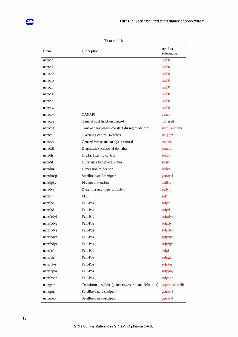
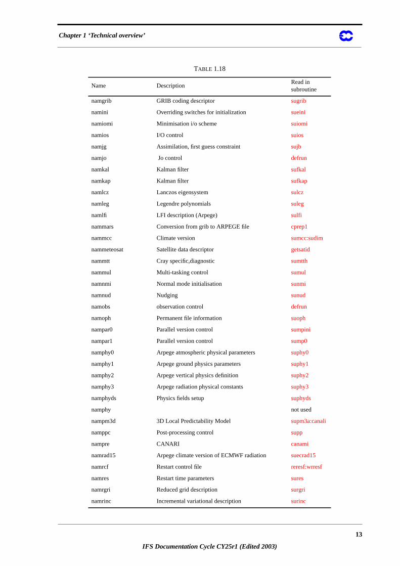
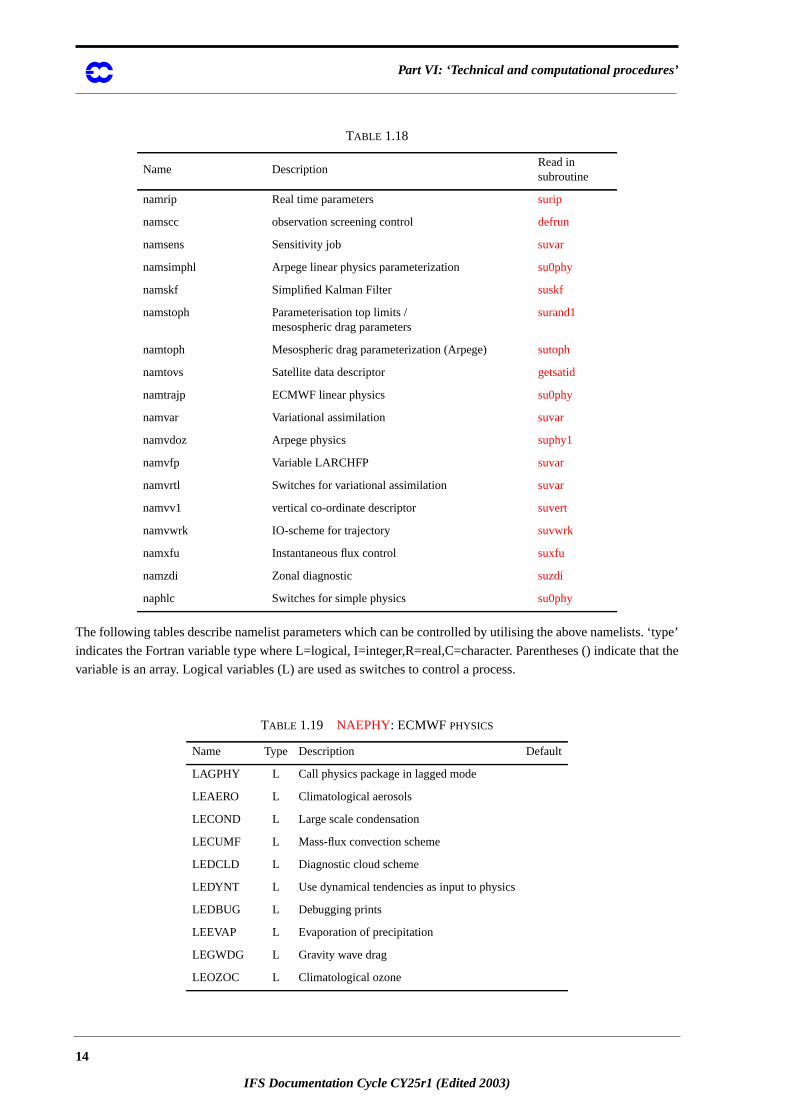
1.6.1 Index of Namelists
TABLE 1.18
Name DescriptionRead insubroutine
nacobs CANARI defrun
nactdo CANARI not used
nactex CANARI canali
nacveg CANARI canali
naephy ECMWF physics su0phy
naerad ECMWF radiation suecrad
naimpo CANARI canali
nalori CANARI canali
nam926 Change of orography su926
nam_distributed_vectors Initialize chunksize forDistributed Vectors
sumpini
namafn Full-Pos suafn
namana CANARI canali:defrun
namcfu Flux accumulation control sucfu
namchk Gridpoint evolution diagnostics suechk
namcla incli0
namclb incli0
11
IFS Documentation Cycle CY25r1 (Edited 2003)
Part VI: ‘Technical and computational procedures’
namclc incli0
namcli incli0
namclo incli0
namclp incli0
namclr incli0
namcls incli0
namclt incli0
namclw incli0
namcok CANARI canali
namcos General cost function control not used
namct0 Control parameters, constant during model run suct0:sumpini
namct1 Overiding control switches su1yom
namcva General variational analysis control sualctv
namddh Diagnostic (horizontal domain) sunddh
namdfi Digital filtering control suedfi
namdif Difference two model states sudif
namdim Dimension/truncation sudim
namdmsp Satellite data descriptor getsatid
namdphy Physics dimension sudim
namdyn Dynamics and hyperdiffusion sudyn
namfft FFT sufft
namfpc Full-Pos sufpc
namfpd Full-Pos sufpd
namfpdyh Full-Pos sufpdyn
namfpdyp Full-Pos sufpdyn
namfpdys Full-Pos sufpdyn
namfpdyt Full-Pos sufpdyn
namfpdyv Full-Pos sufpdyn
namfpf Full-Pos sufpf
namfpg Full-Pos sufpg1
namfpios Full-Pos sufpios
namfpphy Full-Pos sufpphy
namfpsc2 Full-Pos sufpsc2
namgem Transformed sphere (geometry/coordinate definition)sugem1a:inclib
namgms Satellite data descriptor getsatid
namgoes Satellite data descriptor getsatid
TABLE 1.18
Name DescriptionRead insubroutine
12
IFS Documentation Cycle CY25r1 (Edited 2003)
Chapter 1 ‘Technical overview’
namgrib GRIB coding descriptor sugrib
namini Overriding switches for initialization sueini
namiomi Minimisation i/o scheme suiomi
namios I/O control suios
namjg Assimilation, first guess constraint sujb
namjo Jo control defrun
namkal Kalman filter sufkal
namkap Kalman filter sufkap
namlcz Lanczos eigensystem sulcz
namleg Legendre polynomials suleg
namlfi LFI description (Arpege) sulfi
nammars Conversion from grib to ARPEGE file cprep1
nammcc Climate version sumcc:sudim
nammeteosat Satellite data descriptor getsatid
nammtt Cray specific,diagnostic sumtth
nammul Multi-tasking control sumul
namnmi Normal mode initialisation sunmi
namnud Nudging sunud
namobs observation control defrun
namoph Permanent file information suoph
nampar0 Parallel version control sumpini
nampar1 Parallel version control sump0
namphy0 Arpege atmospheric physical parameters suphy0
namphy1 Arpege ground physics parameters suphy1
namphy2 Arpege vertical physics definition suphy2
namphy3 Arpege radiation physical constants suphy3
namphyds Physics fields setup suphyds
namphy not used
nampm3d 3D Local Predictability Model supm3a:canali
namppc Post-processing control supp
nampre CANARI canami
namrad15 Arpege climate version of ECMWF radiation suecrad15
namrcf Restart control file reresf:wrresf
namres Restart time parameters sures
namrgri Reduced grid description surgri
namrinc Incremental variational description surinc
TABLE 1.18
Name DescriptionRead insubroutine
13
IFS Documentation Cycle CY25r1 (Edited 2003)
Part VI: ‘Technical and computational procedures’
. ‘type’
that the
The following tables describe namelist parameters which can be controlled by utilising the above namelists
indicates the Fortran variable type where L=logical, I=integer,R=real,C=character. Parentheses () indicate
variable is an array. Logical variables (L) are used as switches to control a process.
namrip Real time parameters surip
namscc observation screening control defrun
namsens Sensitivity job suvar
namsimphl Arpege linear physics parameterization su0phy
namskf Simplified Kalman Filter suskf
namstoph Parameterisation top limits /mesospheric drag parameters
surand1
namtoph Mesospheric drag parameterization (Arpege) sutoph
namtovs Satellite data descriptor getsatid
namtrajp ECMWF linear physics su0phy
namvar Variational assimilation suvar
namvdoz Arpege physics suphy1
namvfp Variable LARCHFP suvar
namvrtl Switches for variational assimilation suvar
namvv1 vertical co-ordinate descriptor suvert
namvwrk IO-scheme for trajectory suvwrk
namxfu Instantaneous flux control suxfu
namzdi Zonal diagnostic suzdi
naphlc Switches for simple physics su0phy
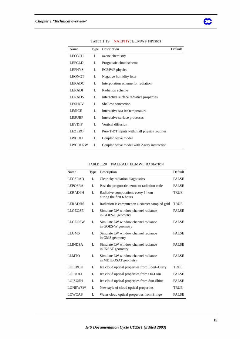
TABLE 1.19 NAEPHY: ECMWF PHYSICS
Name Type Description Default
LAGPHY L Call physics package in lagged mode
LEAERO L Climatological aerosols
LECOND L Large scale condensation
LECUMF L Mass-flux convection scheme
LEDCLD L Diagnostic cloud scheme
LEDYNT L Use dynamical tendencies as input to physics
LEDBUG L Debugging prints
LEEVAP L Evaporation of precipitation
LEGWDG L Gravity wave drag
LEOZOC L Climatological ozone
TABLE 1.18
Name DescriptionRead insubroutine
14
IFS Documentation Cycle CY25r1 (Edited 2003)
Chapter 1 ‘Technical overview’
LEO3CH L ozone chemistry
LEPCLD L Prognostic cloud scheme
LEPHYS L ECMWF physics
LEQNGT L Negative humidity fixer
LERADC L Interpolation scheme for radiation
LERADI L Radiation scheme
LERADS L Interactive surface radiative properties
LESHCV L Shallow convection
LESICE L Interactive sea ice temperature
LESURF L Interactive surface processes
LEVDIF L Vertical diffusion
LEZERO L Pure T-DT inputs within all physics routines
LWCOU L Coupled wave model
LWCOU2W L Coupled wave model with 2-way interaction
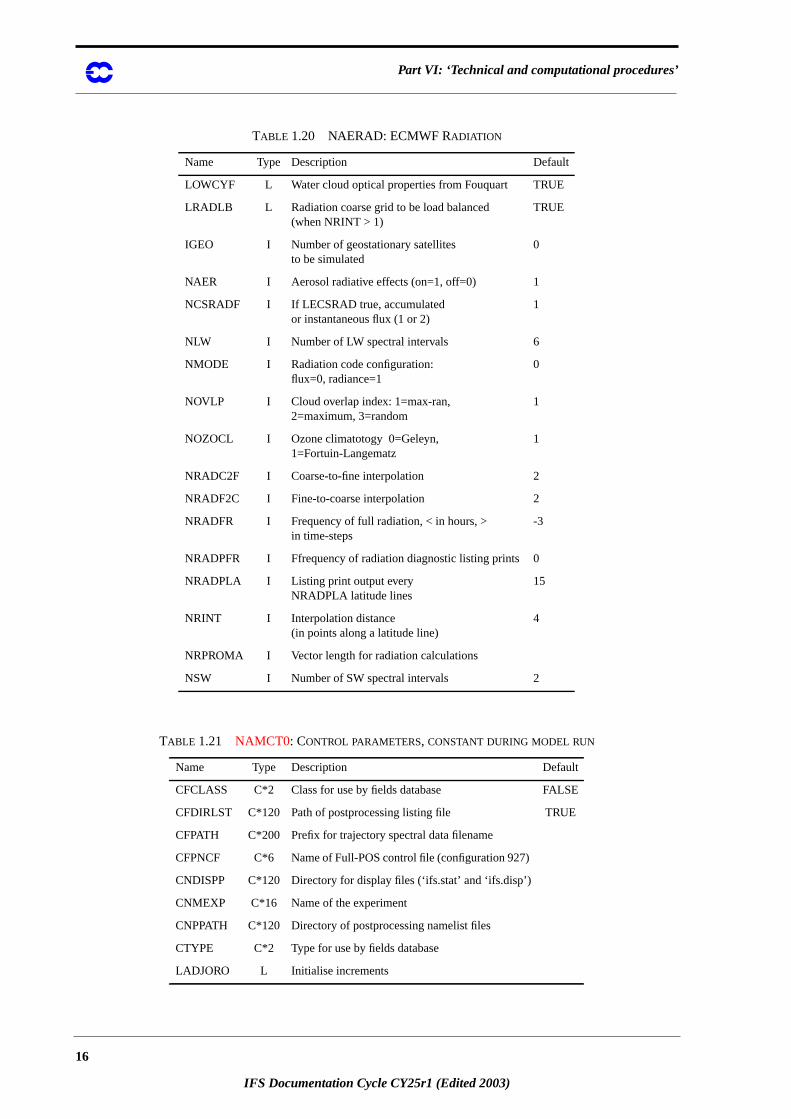
TABLE 1.20 NAERAD: ECMWF RADIATION
Name Type Description Default
LECSRAD L Clear-sky radiation diagnostics FALSE
LEPO3RA L Pass the prognostic ozone to radiation code FALSE
LERAD6H L Radiative computations every 1 hourduring the first 6 hours
TRUE
LERADHS L Radiation is computedon a coarser sampled grid TRUE
LLGEOSE L Simulate LW window channel radiancein GOES-E geometry
FALSE
LLGEOSW L Simulate LW window channel radiancein GOES-W geometry
FALSE
LLGMS L Simulate LW window channel radiancein GMS geometry
FALSE
LLINDSA L Simulate LW window channel radiancein INSAT geometry
FALSE
LLMTO L Simulate LW window channel radiancein METEOSAT geometry
FALSE
LOIEBCU L Ice cloud optical properties from Ebert–Curry TRUE
LOIOULI L Ice cloud optical properties from Ou-Liou FALSE
LOISUSH L Ice cloud optical properties from Sun-Shine FALSE
LONEWSW L New style of cloud optical properties TRUE
LOWCAS L Water cloud optical properties from Slingo FALSE
TABLE 1.19 NAEPHY: ECMWF PHYSICS
Name Type Description Default
15
IFS Documentation Cycle CY25r1 (Edited 2003)
Part VI: ‘Technical and computational procedures’
LOWCYF L Water cloud optical properties from Fouquart TRUE
LRADLB L Radiation coarse grid to be load balanced(when NRINT > 1)
TRUE
IGEO I Number of geostationary satellitesto be simulated
0
NAER I Aerosol radiative effects (on=1, off=0) 1
NCSRADF I If LECSRAD true, accumulatedor instantaneous flux (1 or 2)
1
NLW I Number of LW spectral intervals 6
NMODE I Radiation code configuration:flux=0, radiance=1
0
NOVLP I Cloud overlap index: 1=max-ran,2=maximum, 3=random
1
NOZOCL I Ozone climatotogy 0=Geleyn,1=Fortuin-Langematz
1
NRADC2F I Coarse-to-fine interpolation 2
NRADF2C I Fine-to-coarse interpolation 2
NRADFR I Frequency of full radiation, < in hours, >in time-steps
-3
NRADPFR I Ffrequency of radiation diagnostic listing prints 0
NRADPLA I Listing print output everyNRADPLA latitude lines
15
NRINT I Interpolation distance(in points along a latitude line)
4
NRPROMA I Vector length for radiation calculations
NSW I Number of SW spectral intervals 2
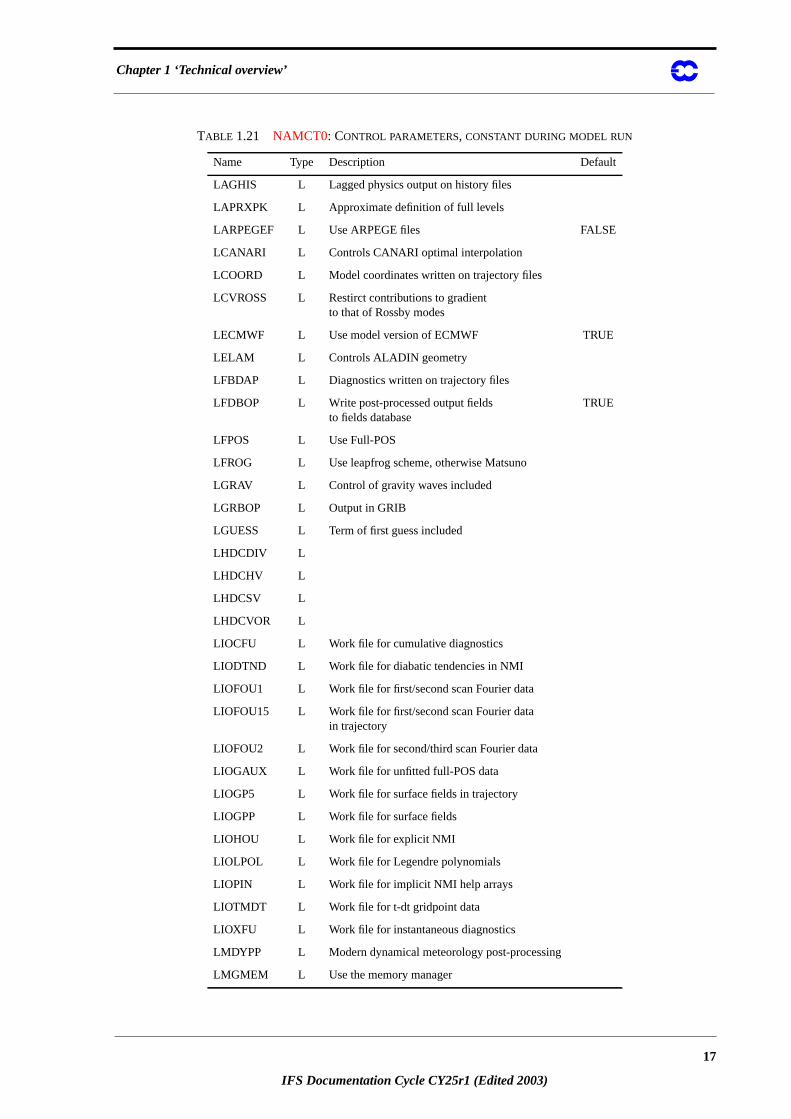
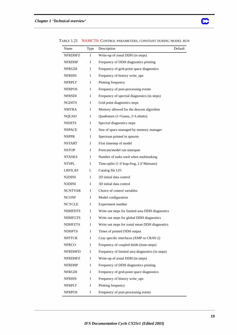
TABLE 1.21 NAMCT0: CONTROL PARAMETERS, CONSTANT DURING MODEL RUN
Name Type Description Default
CFCLASS C*2 Class for use by fields database FALSE
CFDIRLST C*120 Path of postprocessing listing file TRUE
CFPATH C*200 Prefix for trajectory spectral data filename
CFPNCF C*6 Name of Full-POS control file (configuration 927)
CNDISPP C*120 Directory for display files (‘ifs.stat’ and ‘ifs.disp’)
CNMEXP C*16 Name of the experiment
CNPPATH C*120 Directory of postprocessing namelist files
CTYPE C*2 Type for use by fields database
LADJORO L Initialise increments
TABLE 1.20 NAERAD: ECMWF RADIATION
Name Type Description Default
16
IFS Documentation Cycle CY25r1 (Edited 2003)
Chapter 1 ‘Technical overview’
LAGHIS L Lagged physics output on history files
LAPRXPK L Approximate definition of full levels
LARPEGEF L Use ARPEGE files FALSE
LCANARI L Controls CANARI optimal interpolation
LCOORD L Model coordinates written on trajectory files
LCVROSS L Restirct contributions to gradientto that of Rossby modes
LECMWF L Use model version of ECMWF TRUE
LELAM L Controls ALADIN geometry
LFBDAP L Diagnostics written on trajectory files
LFDBOP L Write post-processed output fieldsto fields database
TRUE
LFPOS L Use Full-POS
LFROG L Use leapfrog scheme, otherwise Matsuno
LGRAV L Control of gravity waves included
LGRBOP L Output in GRIB
LGUESS L Term of first guess included
LHDCDIV L
LHDCHV L
LHDCSV L
LHDCVOR L
LIOCFU L Work file for cumulative diagnostics
LIODTND L Work file for diabatic tendencies in NMI
LIOFOU1 L Work file for first/second scan Fourier data
LIOFOU15 L Work file for first/second scan Fourier datain trajectory
LIOFOU2 L Work file for second/third scan Fourier data
LIOGAUX L Work file for unfitted full-POS data
LIOGP5 L Work file for surface fields in trajectory
LIOGPP L Work file for surface fields
LIOHOU L Work file for explicit NMI
LIOLPOL L Work file for Legendre polynomials
LIOPIN L Work file for implicit NMI help arrays
LIOTMDT L Work file for t-dt gridpoint data
LIOXFU L Work file for instantaneous diagnostics
LMDYPP L Modern dynamical meteorology post-processing
LMGMEM L Use the memory manager
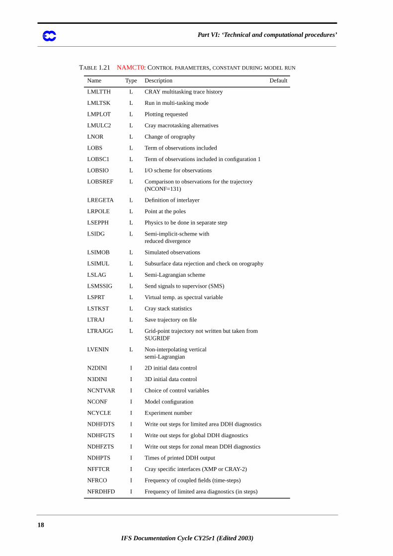
TABLE 1.21 NAMCT0: CONTROL PARAMETERS, CONSTANT DURING MODEL RUN
Name Type Description Default
17
IFS Documentation Cycle CY25r1 (Edited 2003)
Part VI: ‘Technical and computational procedures’
LMLTTH L CRAY multitasking trace history
LMLTSK L Run in multi-tasking mode
LMPLOT L Plotting requested
LMULC2 L Cray macrotasking alternatives
LNOR L Change of orography
LOBS L Term of observations included
LOBSC1 L Term of observations included in configuration 1
LOBSIO L I/O scheme for observations
LOBSREF L Comparison to observations for the trajectory(NCONF=131)
LREGETA L Definition of interlayer
LRPOLE L Point at the poles
LSEPPH L Physics to be done in separate step
LSIDG L Semi-implicit-scheme withreduced divergence
LSIMOB L Simulated observations
LSIMUL L Subsurface data rejection and check on orography
LSLAG L Semi-Lagrangian scheme
LSMSSIG L Send signals to supervisor (SMS)
LSPRT L Virtual temp. as spectral variable
LSTKST L Cray stack statistics
LTRAJ L Save trajectory on file
LTRAJGG L Grid-point trajectory not written but taken fromSUGRIDF
LVENIN L Non-interpolating verticalsemi-Lagrangian
N2DINI I 2D initial data control
N3DINI I 3D initial data control
NCNTVAR I Choice of control variables
NCONF I Model configuration
NCYCLE I Experiment number
NDHFDTS I Write out steps for limited area DDH diagnostics
NDHFGTS I Write out steps for global DDH diagnostics
NDHFZTS I Write out steps for zonal mean DDH diagnostics
NDHPTS I Times of printed DDH output
NFFTCR I Cray specific interfaces (XMP or CRAY-2)
NFRCO I Frequency of coupled fields (time-steps)
NFRDHFD I Frequency of limited area diagnostics (in steps)
TABLE 1.21 NAMCT0: CONTROL PARAMETERS, CONSTANT DURING MODEL RUN
Name Type Description Default
18
IFS Documentation Cycle CY25r1 (Edited 2003)
Chapter 1 ‘Technical overview’
NFRDHFZ I Write-up of zonal DDH (in steps)
NFRDHP I Frequency of DDH diagnostics printing
NFRGDI I Frequency of grid-point space diagnostics
NFRHIS I Frequency of history write_ups
NFRPLT I Plotting frequency
NFRPOS I Frequency of post-processing events
NFRSDI I Frequency of spectral diagnostics (in steps)
NGDITS I Grid point diagnostics steps
NMTRA I Memory allowed for the descent algorithm
NQUAD I Quadrature (1=Gauss, 2=Lobatto)
NSDITS I Spectral diagnostics steps
NSPACE I Size of space managed by memory manager
NSPPR I Spectrum printed in spnorm
NSTART I First timestep of model
NSTOP I Forecast/model run timespan
NTASKS I Number of tasks used when multitasking
NTSPL I Time-splits (1 if leap-frog, 2 if Matsuno)
LRFILAF L Catalog file LFI
N2DINI I 2D initial data control
N3DINI I 3D initial data control
NCNTVAR I Choice of control variables
NCONF I Model configuration
NCYCLE I Experiment number
NDHFDTS I Write out steps for limited area DDH diagnostics
NDHFGTS I Write out steps for global DDH diagnostics
NDHFZTS I Write out steps for zonal mean DDH diagnostics
NDHPTS I Times of printed DDH output
NFFTCR I Cray specific interfaces (XMP or CRAY-2)
NFRCO I Frequency of coupled fields (time-steps)
NFRDHFD I Frequency of limited area diagnostics (in steps)
NFRDHFZ I Write-up of zonal DDH (in steps)
NFRDHP I Frequency of DDH diagnostics printing
NFRGDI I Frequency of grid-point space diagnostics
NFRHIS I Frequency of history write_ups
NFRPLT I Plotting frequency
NFRPOS I Frequency of post-processing events
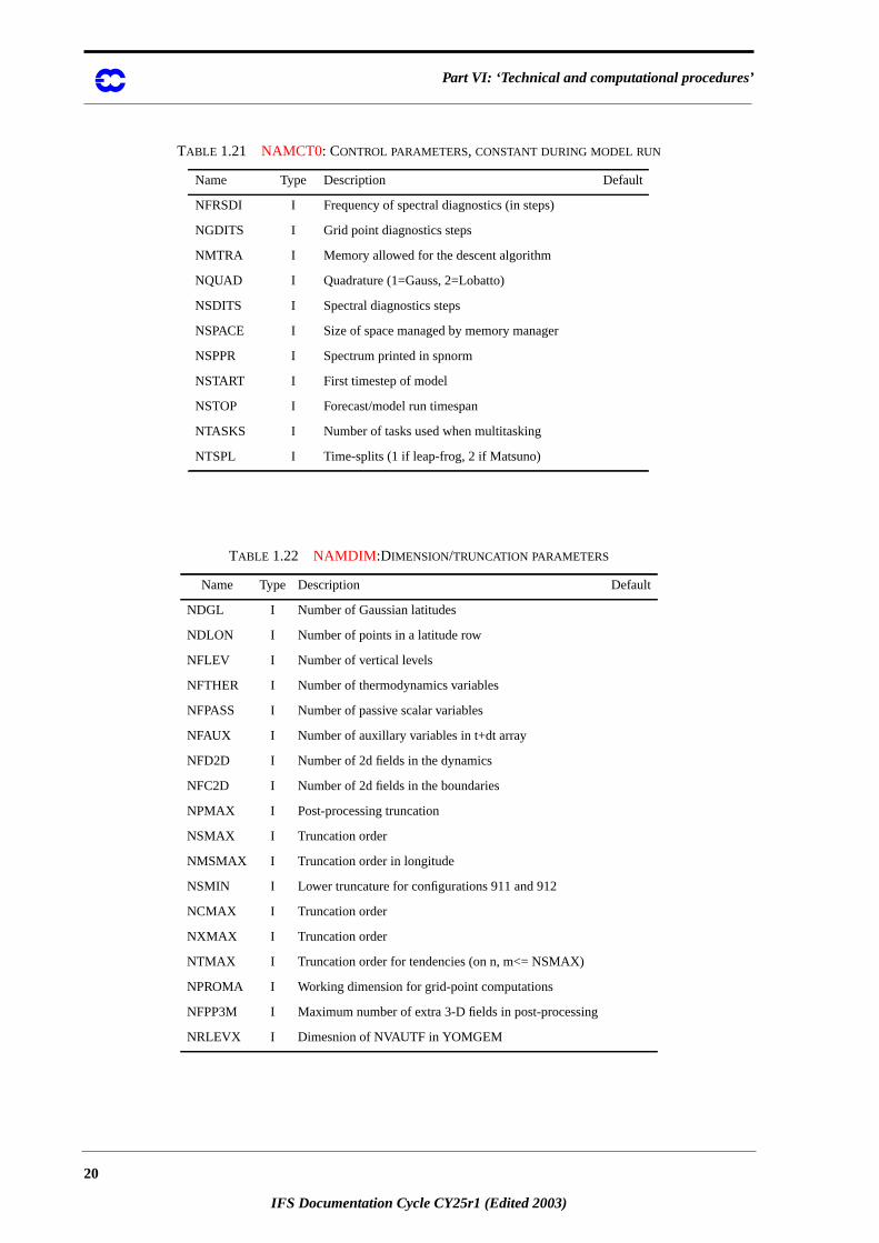
TABLE 1.21 NAMCT0: CONTROL PARAMETERS, CONSTANT DURING MODEL RUN
Name Type Description Default
19
IFS Documentation Cycle CY25r1 (Edited 2003)
Part VI: ‘Technical and computational procedures’
NFRSDI I Frequency of spectral diagnostics (in steps)
NGDITS I Grid point diagnostics steps
NMTRA I Memory allowed for the descent algorithm
NQUAD I Quadrature (1=Gauss, 2=Lobatto)
NSDITS I Spectral diagnostics steps
NSPACE I Size of space managed by memory manager
NSPPR I Spectrum printed in spnorm
NSTART I First timestep of model
NSTOP I Forecast/model run timespan
NTASKS I Number of tasks used when multitasking
NTSPL I Time-splits (1 if leap-frog, 2 if Matsuno)
TABLE 1.22 NAMDIM :DIMENSION/TRUNCATION PARAMETERS
Name Type Description Default
NDGL I Number of Gaussian latitudes
NDLON I Number of points in a latitude row
NFLEV I Number of vertical levels
NFTHER I Number of thermodynamics variables
NFPASS I Number of passive scalar variables
NFAUX I Number of auxillary variables in t+dt array
NFD2D I Number of 2d fields in the dynamics
NFC2D I Number of 2d fields in the boundaries
NPMAX I Post-processing truncation
NSMAX I Truncation order
NMSMAX I Truncation order in longitude
NSMIN I Lower truncature for configurations 911 and 912
NCMAX I Truncation order
NXMAX I Truncation order
NTMAX I Truncation order for tendencies (on n, m<= NSMAX)
NPROMA I Working dimension for grid-point computations
NFPP3M I Maximum number of extra 3-D fields in post-processing
NRLEVX I Dimesnion of NVAUTF in YOMGEM
TABLE 1.21 NAMCT0: CONTROL PARAMETERS, CONSTANT DURING MODEL RUN
Name Type Description Default
20
IFS Documentation Cycle CY25r1 (Edited 2003)
Chapter 1 ‘Technical overview’
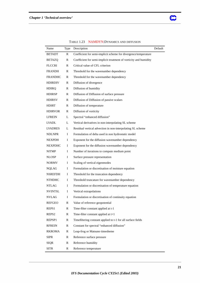
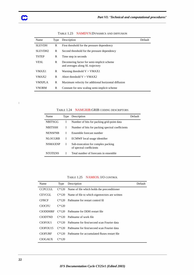
TABLE 1.23 NAMDYN :DYNAMICS AND DIFFUSION
Name Type Description Default
BETADT R Coefficient for semi-implicit scheme for divergence/temperature
BETAZQ R Coefficient for semi-implicit treatment of vorticity and humidity
FLCCRI R Critical value of CFL criterion
FRANDH R Threshold for the wavenumber dependency
FRANDHC R Threshold for the wavenumber dependency
HDIRDIV R Diffusion of divergence
HDIRQ R Diffusion of humidity
HDIRSP R Diffusion of Diffusion of surface pressure
HDIRSV R Diffusion of Diffusion of passive scalars
HDIRT R Diffusion of temperature
HDIRVOR R Diffusion of vorticity
LFREIN L Spectral “enhanced diffusion”
LVADL L Vertical derivatives in non-interpolating SL scheme
LVADRES L Residual vertical advection in non-interpolating SL scheme
NDLNPR I Formulation of delta used in non hydrostatic model
NEXPDH I Exponent for the diffusion wavenumber dependency
NEXPDHC I Exponent for the diffusion wavenumber dependency
NITMP I Number of iterations to compute medium point
NLOSP I Surface pressure representation
NORMV I Scaling of vertical eigenmodes
NQLAG I Formulation or discretisation of moisture equation
NSREFDH I Threshold for the truncation dependency
NTHDHC I Threshold truncature for wavenumber dependency
NTLAG I Formulation or discretisation of temperature equation
NVINTSL I Vertical extrapolations
NVLAG I Formulation or discretisation of continuity equation
REFGEO R Value of reference geopotential
REPS1 R Time-filter constant applied at t-1
REPS2 R Time-filter constant applied at t+1
REPSP1 R Timefiltering constant applied to t-1 for all surface fields
RFREIN R Constant for spectral “enhanced diffusion”
RKROMA R Leap-frog or Matsuno timesheme
SIPR R Reference surface pressure
SIQR R Reference humidity
SITR R Reference temperature
21
IFS Documentation Cycle CY25r1 (Edited 2003)
Part VI: ‘Technical and computational procedures’
:
SLEVDH R First threshold for the pressure dependency
SLEVDH2 R Second threshold for the pressure dependency
TSTEP R Time step in seconds
VESL R Decentering factor for semi-implicit schemeand averages along SL trajectory
VMAX1 R Warning threshold V > VMAX1
VMAX2 R Abort threshold V > VMAX2
VMXPLA R Maximum velocity for additional horizontal diffusion
VNORM R Constant for new scaling semi-implicit scheme
TABLE 1.24 NAMGRIB:GRIB CODING DESCRIPTORS
Name Type Description Default
NBITSGG I Number of bits for packing grid-point data
NBITSSH I Number of bits for packing spectral coefficients
NENSFNB I Ensemble forecast number
NLOCGRB I ECMWF local usage identifier
NSMAXNP I Sub-truncation for complex packingof spectral coefficients
NTOTENS I Total number of forecasts in ensemble
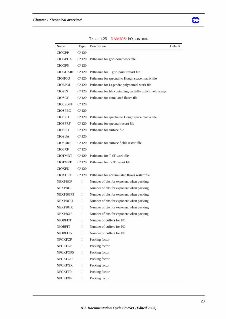
TABLE 1.25 NAMIOS: I/O CONTROL
Name Type Description Default
CCPCCGL C*120 Name of file which holds the preconditioner
CEVCGL C*120 Name of file to which eigenvectors are written
CFRCF C*120 Pathname for restart control fil
CIOCFU C*120
CIODDHRF C*120 Pathname for DDH restart file
CIODTND C*120 Pathname of work file
CIOFOU1 C*120 Pathname for first/second scan Fourier data
CIOFOU15 C*120 Pathname for first/second scan Fourier data
CIOFURF C*120 Pathname for accumulated fluxes restart file
CIOGAUX C*120
TABLE 1.23 NAMDYN :DYNAMICS AND DIFFUSION
Name Type Description Default
22
IFS Documentation Cycle CY25r1 (Edited 2003)
Chapter 1 ‘Technical overview’
CIOGPP C*120
CIOGPUA C*120 Pathname for grid-point work file
CIOGP5 C*120
CIOGUARF C*120 Pathname for T grid-point restart file
CIOHOU C*120 Pathname for spectral to Hough space matrix file
CIOLPOL C*120 Pathname for Legendre polynomial work file
CIOPIN C*120 Pathname for file containing partially imlicit help arrays
CIOSCF C*120 Pathname for cumulated fluxes file
CIOSPBUF C*120
CIOSPEC C*120
CIOSPH C*120 Pathname for spectral to Hough space matrix file
CIOSPRF C*120 Pathname for spectral restart file
CIOSSU C*120 Pathname for surface file
CIOSUA C*120
CIOSURF C*120 Pathname for surface fields restart file
CIOSXF C*120
CIOTMDT C*120 Pathname for T-dT work file
CIOTMRF C*120 Pathname for T-dT restart file
CIOXFU C*120
CIOXURF C*120 Pathname for accumulated fluxes restart file
NEXPBCF I Number of bits for exponent when packing
NEXPBGP I Number of bits for exponent when packing
NEXPBGP5 I Number of bits for exponent when packing
NEXPBGU I Number of bits for exponent when packing
NEXPBGX I Number of bits for exponent when packing
NEXPBXF I Number of bits for exponent when packing
NIOBFDT I Number of buffers for I/O
NIOBFIT I Number of buffers for I/O
NIOBFIT5 I Number of buffers for I/O
NPCKFCF I Packing factor
NPCKFGP I Packing factor
NPCKFGP5 I Packing factor
NPCKFGU I Packing factor
NPCKFGX I Packing factor
NPCKFT9 I Packing factor
NPCKFXF I Packing factor
TABLE 1.25 NAMIOS: I/O CONTROL
Name Type Description Default
23
IFS Documentation Cycle CY25r1 (Edited 2003)
Part VI: ‘Technical and computational procedures’
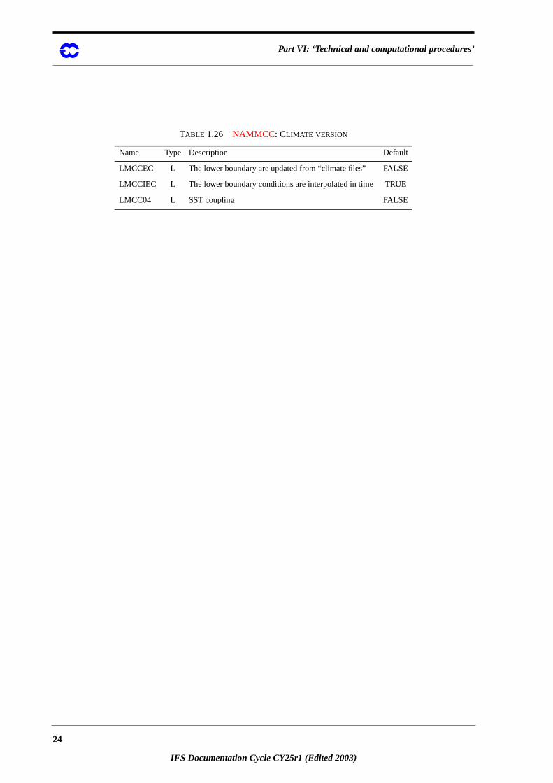
TABLE 1.26 NAMMCC: CLIMATE VERSION
Name Type Description Default
LMCCEC L The lower boundary are updated from “climate files” FALSE
LMCCIEC L The lower boundary conditions are interpolated in time TRUE
LMCC04 L SST coupling FALSE
24
IFS Documentation Cycle CY25r1 (Edited 2003)
Chapter 1 ‘Technical overview’
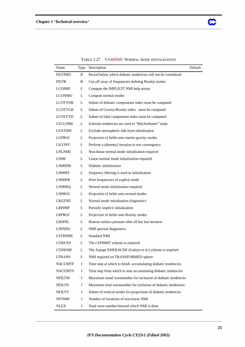
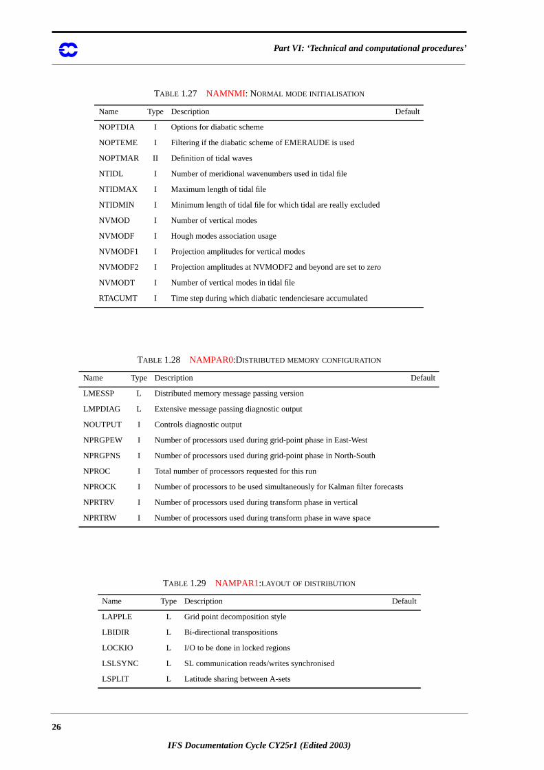
TABLE 1.27 NAMNMI : NORMAL MODE INITIALISATION
Name Type Description Default
FILTPRD R Period below which diabatic tendencies will not be considered
FILTR R Cut-off array of frequencies defining Rossby modes
LCOIMP L Compute the IMPLICIT NMI help arrays
LCONMO L Compute normal modes
LCOTYDB L Subset of diabatic components index must be computed
LCOTYGR L Subset of Gravity/Rossby index must be computed
LCOTYTD L Subset of tidal components index must be computed
LEULNMI L Eulerian tendencies are used in “Machenhauer” steps
LEXTIDE L Exclude atmospheric tide from initialisation
LGPROJ L Projection of fields onto inertia-gravity modes
LICONV L Perform a (dummy) iteration to test convergence
LNLNMI L Non-linear normal mode initialisation required
LNMI L Linear normal mode initialisation required
LNMIDB L Diabatic initialization
LNMIFF L frequency filtering is used in initialization
LNMIPR L Print frequencies of explicit mode
LNMIRQ L Normal mode initialisation required
LNPROJ L Projection of fields onto normal modes
LRGENE L Normal mode initialisation diagnostics
LRPIMP L Partially implicit initialisation
LRPROJ L Projection of fields onto Rossby modes
LRSPSL L Restore surface pressure after all but last iteration
LSPNDG L NMI spectral diagnostics
LSTDNMI L Standard NMI
LTIDCEP L The CEPMMT scheme is required
LTIDEME L The Arpege EMERAUDE (Geleyn et al.) scheme is required
LTRANS L NMI required on TRANSFORMED sphere
NACUMTF I Time step at which to finish accumulating diabatic tendencies
NACUMTS I Time step from which to start accumulating diabatic tendencies
NFILTM I Maximum zonal wavenumber for inclusion of diabatic tendencies
NFILTN I Maximum total wavenumber for inclusion of diabatic tendencies
NFILTV I Subset of vertical modes for projections of diabatic tendencies
NITNMI I Number of iterations of non-linear NMI
NLEX I Total wave number beyond which NMI is done
25
IFS Documentation Cycle CY25r1 (Edited 2003)
Part VI: ‘Technical and computational procedures’
NOPTDIA I Options for diabatic scheme
NOPTEME I Filtering if the diabatic scheme of EMERAUDE is used
NOPTMAR II Definition of tidal waves
NTIDL I Number of meridional wavenumbers used in tidal file
NTIDMAX I Maximum length of tidal file
NTIDMIN I Minimum length of tidal file for which tidal are really excluded
NVMOD I Number of vertical modes
NVMODF I Hough modes association usage
NVMODF1 I Projection amplitudes for vertical modes
NVMODF2 I Projection amplitudes at NVMODF2 and beyond are set to zero
NVMODT I Number of vertical modes in tidal file
RTACUMT I Time step during which diabatic tendenciesare accumulated
TABLE 1.28 NAMPAR0:DISTRIBUTED MEMORY CONFIGURATION
Name Type Description Default
LMESSP L Distributed memory message passing version
LMPDIAG L Extensive message passing diagnostic output
NOUTPUT I Controls diagnostic output
NPRGPEW I Number of processors used during grid-point phase in East-West
NPRGPNS I Number of processors used during grid-point phase in North-South
NPROC I Total number of processors requested for this run
NPROCK I Number of processors to be used simultaneously for Kalman filter forecasts
NPRTRV I Number of processors used during transform phase in vertical
NPRTRW I Number of processors used during transform phase in wave space
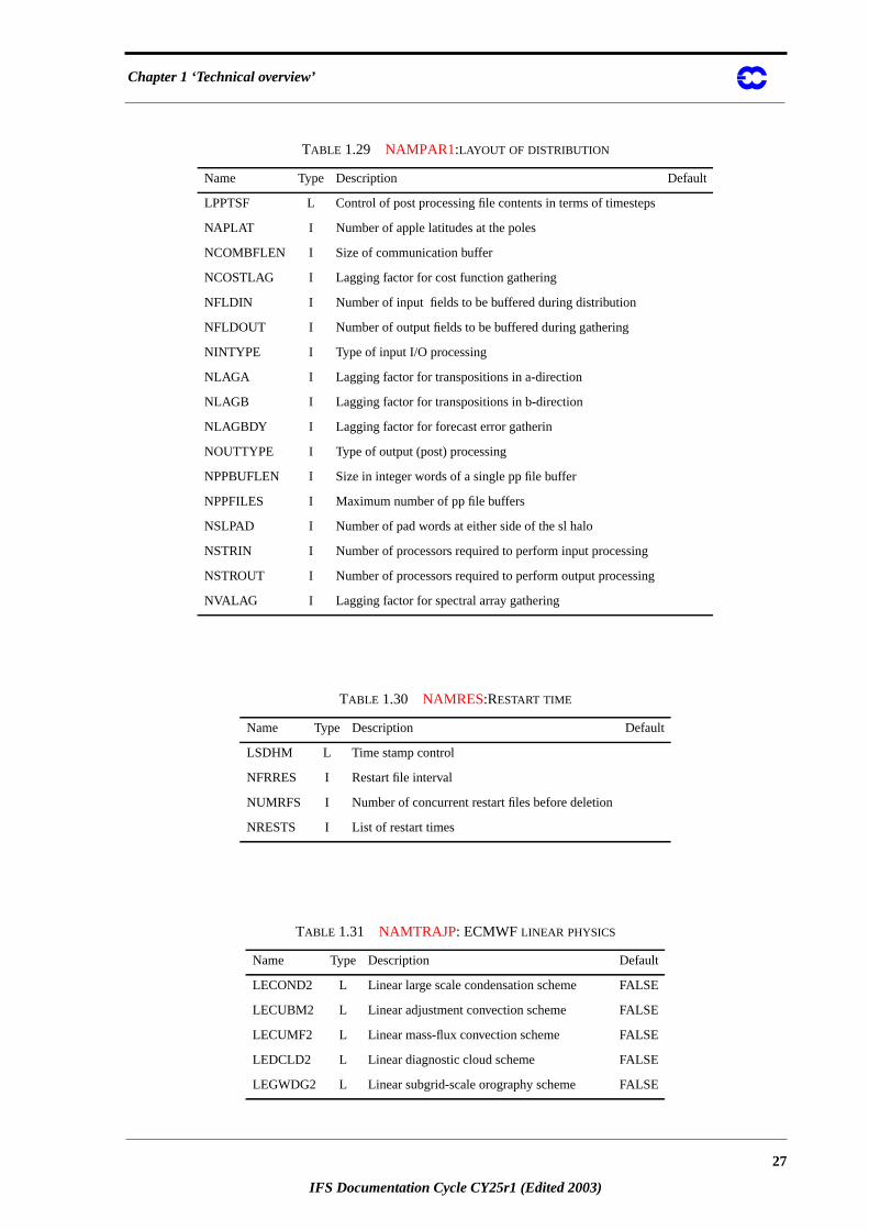
TABLE 1.29 NAMPAR1:LAYOUT OF DISTRIBUTION
Name Type Description Default
LAPPLE L Grid point decomposition style
LBIDIR L Bi-directional transpositions
LOCKIO L I/O to be done in locked regions
LSLSYNC L SL communication reads/writes synchronised
LSPLIT L Latitude sharing between A-sets
TABLE 1.27 NAMNMI : NORMAL MODE INITIALISATION
Name Type Description Default
26
IFS Documentation Cycle CY25r1 (Edited 2003)
Chapter 1 ‘Technical overview’
LPPTSF L Control of post processing file contents in terms of timesteps
NAPLAT I Number of apple latitudes at the poles
NCOMBFLEN I Size of communication buffer
NCOSTLAG I Lagging factor for cost function gathering
NFLDIN I Number of input fields to be buffered during distribution
NFLDOUT I Number of output fields to be buffered during gathering
NINTYPE I Type of input I/O processing
NLAGA I Lagging factor for transpositions in a-direction
NLAGB I Lagging factor for transpositions in b-direction
NLAGBDY I Lagging factor for forecast error gatherin
NOUTTYPE I Type of output (post) processing
NPPBUFLEN I Size in integer words of a single pp file buffer
NPPFILES I Maximum number of pp file buffers
NSLPAD I Number of pad words at either side of the sl halo
NSTRIN I Number of processors required to perform input processing
NSTROUT I Number of processors required to perform output processing
NVALAG I Lagging factor for spectral array gathering
TABLE 1.30 NAMRES:RESTART TIME
Name Type Description Default
LSDHM L Time stamp control
NFRRES I Restart file interval
NUMRFS I Number of concurrent restart files before deletion
NRESTS I List of restart times
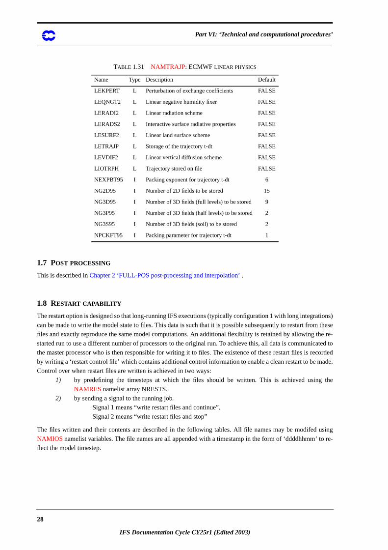
TABLE 1.31 NAMTRAJP: ECMWF LINEAR PHYSICS
Name Type Description Default
LECOND2 L Linear large scale condensation scheme FALSE
LECUBM2 L Linear adjustment convection scheme FALSE
LECUMF2 L Linear mass-flux convection scheme FALSE
LEDCLD2 L Linear diagnostic cloud scheme FALSE
LEGWDG2 L Linear subgrid-scale orography scheme FALSE
TABLE 1.29 NAMPAR1:LAYOUT OF DISTRIBUTION
Name Type Description Default
27
IFS Documentation Cycle CY25r1 (Edited 2003)
Part VI: ‘Technical and computational procedures’
tions)
m these
he re-
ated to
corded
ade.
the
using
to re-
1.7 POST PROCESSING
This is described inChapter 2 ‘FULL-POS post-processing and interpolation’ .
1.8 RESTART CAPABILITY
The restart option is designed so that long-running IFS executions (typically configuration 1 with long integra
can be made to write the model state to files. This data is such that it is possible subsequently to restart fro
files and exactly reproduce the same model computations. An additional flexibility is retained by allowing t
started run to use a different number of processors to the original run. To achieve this, all data is communic
the master processor who is then responsible for writing it to files. The existence of these restart files is re
by writing a ‘restart control file’ which contains additional control information to enable a clean restart to be m
Control over when restart files are written is achieved in two ways:
1) by predefining the timesteps at which the files should be written. This is achieved using
NAMRES namelist array NRESTS.
2) by sending a signal to the running job.
Signal 1 means “write restart files and continue”.
Signal 2 means “write restart files and stop”
The files written and their contents are described in the following tables. All file names may be modifed
NAMIOS namelist variables. The file names are all appended with a timestamp in the form of ‘ddddhhmm’
flect the model timestep.
LEKPERT L Perturbation of exchange coefficients FALSE
LEQNGT2 L Linear negative humidity fixer FALSE
LERADI2 L Linear radiation scheme FALSE
LERADS2 L Interactive surface radiative properties FALSE
LESURF2 L Linear land surface scheme FALSE
LETRAJP L Storage of the trajectory t-dt FALSE
LEVDIF2 L Linear vertical diffusion scheme FALSE
LIOTRPH L Trajectory stored on file FALSE
NEXPBT95 I Packing exponent for trajectory t-dt 6
NG2D95 I Number of 2D fields to be stored 15
NG3D95 I Number of 3D fields (full levels) to be stored 9
NG3P95 I Number of 3D fields (half levels) to be stored 2
NG3S95 I Number of 3D fields (soil) to be stored 2
NPCKFT95 I Packing parameter for trajectory t-dt 1
TABLE 1.31 NAMTRAJP: ECMWF LINEAR PHYSICS
Name Type Description Default
28
IFS Documentation Cycle CY25r1 (Edited 2003)
Chapter 1 ‘Technical overview’
e used
on
E
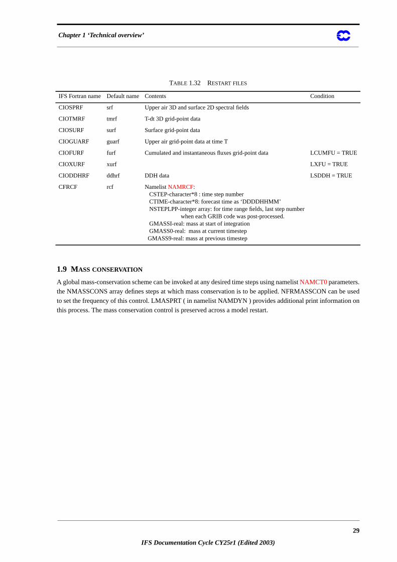
1.9 MASS CONSERVATION
A global mass-conservation scheme can be invoked at any desired time steps using namelistNAMCT0 parameters.
the NMASSCONS array defines steps at which mass conservation is to be applied. NFRMASSCON can b
to set the frequency of this control. LMASPRT ( in namelist NAMDYN ) provides additional print information
this process. The mass conservation control is preserved across a model restart.
TABLE 1.32 RESTART FILES
IFS Fortran name Default name Contents Condition
CIOSPRF srf Upper air 3D and surface 2D spectral fields
CIOTMRF tmrf T-dt 3D grid-point data
CIOSURF surf Surface grid-point data
CIOGUARF guarf Upper air grid-point data at time T
CIOFURF furf Cumulated and instantaneous fluxes grid-point data LCUMFU = TRU
CIOXURF xurf LXFU = TRUE
CIODDHRF ddhrf DDH data LSDDH = TRUE
CFRCF rcf NamelistNAMRCF:CSTEP-character*8 : time step numberCTIME-character*8: forecast time as ‘DDDDHHMM’NSTEPLPP-integer array: for time range fields, last step number
when each GRIB code was post-processed.GMASSI-real: mass at start of integrationGMASS0-real: mass at current timestepGMASS9-real: mass at previous timestep
29
IFS Documentation Cycle CY25r1 (Edited 2003)

Part VI: ‘Technical and computational procedures’
30
IFS Documentation Cycle CY25r1 (Edited 2003)
IFS Documentation Cycle CY25r1
Part VI: T ECHNICAL AND COMPUTATIONAL PROCEDURES
CHAPTER 2 FULL-POS post-processing andinterpolationThis documentation describes the FULL-POS functionality of ARPEGE/IFS .
Table of contents
2.1 Post-processable fields.
2.1.1 3D dynamical fields (DYN3D).
2.1.2 2D dynamical fields (DYN2D).
2.1.3 Surface physical fields (PHYSOL) used both at METEO-FRANCE and ECMWF.
2.1.4 Additional surface physical fields (PHYSOL) used only at ECMWF.
2.1.5 Surface cumulated fluxes (CFU).
2.1.6 Surface instantaneous fluxes (XFU).
2.2 Other notations.
2.3 Horizontal interpolations.
2.3.1 Bilinear horizontal interpolations.
2.3.2 12 points horizontal interpolations.
2.3.3 Location of computations.
2.3.4 Plane geometry (ALADIN).
2.4 Vertical interpolations and extrapolations.
2.4.1 General considerations.
2.4.2 More details for 3D dynamical variables.
2.4.3 2D dynamical variables which need extrapolations.
2.5 Filtering in spectral space.
2.5.1 General considerations.
2.5.2 ‘THX’ (ARPEGE) or bell-shaped (ALADIN) filtering on derivatives.
2.5.3 ‘Bell-shaped’ filtering on non-derivative fields.
2.5.4 Additional ‘THX’ filtering on all fields.
2.6 Post-processing files.
2.7 Organigram
2.7.1 Setup routines and arborescence above STEPO.
2.7.2 Grid-point computations.
31
IFS Documentationn Cycle CY25r1 (Edited 2003)
Part VI: ‘Technical and computational procedures’
metry.
odel
rent
s in
S to
S to
2.7.3 Spectral transforms.
2.7.4 Spectral computations.
2.7.5 Action and brief description of each routine.
2.8 Sequences of calls of post-processing.
2.8.1 Vertical coordinates of post-processing.
2.8.2 Sequences of calls: general considerations.
2.8.3 Global spectral post-processed fields in the same horizontal geometry as the model geo
2.8.4 Global spectral post-processed fields in a horizontal geometry different from the m
geometry.
2.8.5 Global grid-point post-processed fields in the same horizontal geometry or in a diffe
horizontal geometry as the model geometry.
2.8.6 Spectral fit.
2.8.7 No spectral fit.
2.8.8 Grid-point post-processed fields in a ALADIN limited area domain.
2.8.9 Grid-point post-processed fields in a latitude-longitude limited area domain.
2.8.10 Mixed ARPEGE/IFS-ALADIN FULL-POS configurations: spectral post-processed field
a limited area domain.
2.8.11 Pure ALADIN FULL-POS configurations.
2.9 Some shared memory features:
2.9.1 Calculations packets:
2.9.2 Transmission of data necessary for FULL-POS horizontal interpolations from HPO
HPOSLAG: interpolation buffers.
2.10 Some distributed memory features:
2.10.1 Calculations packets:
2.10.2 Transmission of data necessary for FULL-POS horizontal interpolations from HPO
HPOSLAG: interpolation buffers.
2.11 Parameter variables to be known:
2.11.1 Parameter PARFPOS.
2.12 Common/module and namelist variables to be known:
2.12.1 PTRFPB2.
2.12.2 YOM4FPOS.
2.12.3 YOMAFN.
2.12.4 YOMAFPB.
2.12.5 YOMAFPDS.
32
IFS Documentation Cycle CY25r1 (Edited 2003)
Chapter 2 ‘FULL-POS post-processing and interpolation’
2.12.6 YOMCT0.
2.12.7 YOMDFPB.
2.12.8 YOMDIM.
2.12.9 YOMFP4.
2.12.10 YOMFP4L.
2.12.11 YOMFPC.
2.12.12 YOMFPD.
2.12.13 YOMFPF.
2.12.14 YOMFPG.
2.12.15 YOMFPIOS.
2.12.16 YOMFPOLE.
2.12.17 YOMFPOP.
2.12.18 YOMFPSC2.
2.12.19 YOMFPSC2B.
2.12.20 YOMFPSP.
2.12.21 YOMFPT0.
2.12.22 YOMIOS.
2.12.23 YOMMP.
2.12.24 YOMMPG.
2.12.25 YOMOP.
2.12.26 YOMPFPB.
2.12.27 YOMRFPB.
2.12.28 YOMRFPDS.
2.12.29 YOMSC2.
2.12.30 YOMVFP.
2.12.31 YOMVPOS.
2.12.32 YOMWFPB.
2.12.33 YOMWFPDS.
2.12.34 Additional namelists, containing local variables.
2.12.35 Pointer variables to be known:
Pointer PTRFP4.
33
IFS Documentation Cycle CY25r1 (Edited 2003)
Part VI: ‘Technical and computational procedures’
ture lev-
EO-
ly).
2.1 POST-PROCESSABLE FIELDS.
Post-processing can be made on pressure levels, height levels, potential vorticity levels, potential tempera
els or -levels.
2.1.1 3D dynamical fields (DYN3D).• 01) Geopotential .
• 02) Temperature .
• 03 and 04) Horizontal wind components and .
• 05) Specific humidity (moisture) .
• 06) Relative humidity .
• 07) Ice content .
• 08) Pressure coordinate vertical velocity .
• 09) Relative vorticity .
• 10) Divergence .
• 11) Potential temperature .
• 12) Velocity potential (has to be fitted).
• 13) Stream function (has to be fitted).
• 14) Liquid water content .
• 15) Moist (irreversible) pseudo-adiabatic potential temperature .
• 16) Cloud fraction .
• 17) Wind velocity.
• 18) Equivalent potential temperature .
• 19) Absolute vorticity .
• 20) Stretching deformation .
• 21) Shearing deformation .
• 22) Potential vorticity .
• 23) Wet potential vorticity .
• 24 to 26) Passive scalars (maximum of three).
• 27) Pressure .
• 28 to 30) Possibility to post-process three additional free upper air fields nr 1 to 3 (MET
FRANCE and ECMWF).
• 31 to 43) Possibility to post-process 13 additional free upper air fields nr 4 to 16 (ECMWF on
2.1.2 2D dynamical fields (DYN2D).• 01) Surface pressure .
• 02) Mean sea level pressure .
• 03) Interpolated (spectral) model orography.
• 04) Mapping factor .
• 05) Tropopause folding indicator of the iso-2 PVU surface.
• 06) ICAO jet zonal component of wind.
• 07) ICAO jet meridian component of wind.
• 08) Position of ICAO jet in pressure vertical coordinate.
• 09) Position of ICAO tropopause in pressure vertical coordinate.
• 10) ICAO tropopause temperature.
• 11) Logarithm of surface pressure (at ECMWF only).
Remark about fields 06) to 10): at ECMWF they are replaced by some optional surface fields.
η
ΦT
U Vq
HUqi
ωζ
DΘ
ψχ
ql
Θ′wqa
Θe
ζ f+
STDSHD
PVPVw
qSV
Π
Πs
ΠMSL
M
34
IFS Documentation Cycle CY25r1 (Edited 2003)
Chapter 2 ‘FULL-POS post-processing and interpolation’
2.1.3 Surface physical fields (PHYSOL) used both at METEO-FRANCE and ECMWF.• 01) Land/sea mask.
• 02) (Output grid-point orography) .
• 03) Surface temperature.
• 04) Deep soil temperature.
• 05) Interpolated surface temperature.
• 06) Surface soil wetness.
• 07) Deep soil wetness.
• 08) Relaxation deep soil wetness.
• 09) Climatological relative surface soil wetness.
• 10) Climatological relative deep soil wetness.
• 11) Snow depth.
• 12) (Surface roughness) .
• 13) (Roughness length of bare surface) .
• 14) Albedo.
• 15) Emissivity.
• 16) (Standard deviation of orography) .
• 17) Percentage of vegetation.
• 18) Percentage of land.
• 19) Anisotropy coefficient of topography.
• 20) Direction of main axis of topography.
2.1.4 Additional surface physical fields (PHYSOL) used only at ECMWF.• 21) Soil first level temperature.
• 22) Soil first level wetness.
• 23) Soil second level temperature.
• 24) Soil second level wetness.
• 25) Soil third level temperature.
• 26) Soil third level wetness.
• 27) Soil fourth level temperature.
• 28) Soil fourth level wetness.
• 29) Temperature of snow layer.
• 30) Anisotropy of surface orography.
• 31) Angle of surface orography.
• 32) Slope of surface orography.
• 33) Logarithm of surface roughness.
• 34) Skin temperature.
• 35) Apparent surface humidity.
• 36) Skin wetness.
• 37 to 79) Diagnostic fields (not detailed, some of them are present in the CFU and XFU list).
• 80 to 109) Additional optional fields.
2.1.5 Surface cumulated fluxes (CFU).• 01) Large scale precipitation.
• 02) Convective precipitation.
• 03) Large scale snow fall.
• 04) Convective snow fall.
g×
g×g×
g×
35
IFS Documentation Cycle CY25r1 (Edited 2003)
Part VI: ‘Technical and computational procedures’
• 05) -stress.
• 06) -stress.
• 07) Surface sensible heat flux.
• 08) Surface latent heat flux.
• 09) Tendency of surface pressure.
• 10) Total cloud cover.
• 11) Boundary layer dissipation.
• 12) Surface solar radiation.
• 13) Surface thermal radiation.
• 14) Top solar radiation.
• 15) Top thermal radiation.
• 16) Convective cloud cover.
• 17) High cloud cover.
• 18) Medium cloud cover.
• 19) Low cloud cover.
• 20) -gravity-wave stress.
• 21) -gravity-wave stress.
• 22) Water evaporation.
• 23) Snow sublimation.
• 24) Latent heat evaporation.
• 25) Latent heat sublimation.
• 26) Cloudiness.
• 27) Soil moisture.
• 28) Snow mass.
• 29) Total precipitable water.
• 30) Total ozone.
• 31) Top mesospheric enthalpy.
• 32) Solid specific moisture.
• 33) Liquid specific moisture.
• 34) Contribution of convection to .
• 35) Contribution of convection to .
• 36) Contribution of convection to .
• 37) Contribution of convection to .
• 38) Contribution of turbulence to .
• 39) Contribution of turbulence to .
• 40) Clear sky shortwave radiative flux.
• 41) Clear sky longwave radiative flux.
• 42) Surface parallel solar flux.
• 43) Top parallel solar flux.
• 44) Surface down solar flux.
• 45) Surface down thermic flux.
• 46) Melt snow.
• 47) Heat flux in soil.
• 48) Water flux in soil.
• 49) Surface soil runoff.
• 50) Deep soil runoff.
• 51) Interception soil layer runoff.
UV
UV
UVqcpTqcpT
36
IFS Documentation Cycle CY25r1 (Edited 2003)
Chapter 2 ‘FULL-POS post-processing and interpolation’
• 52) Evapotranspiration flux.
• 53) Transpiration flux.
2.1.6 Surface instantaneous fluxes (XFU).• 01) Total cloud cover.
• 02) -component of wind at 10 meters (pbl).
• 03) -component of wind at 10 meters (pbl).
• 04) Temperature at 2 meters (pbl).
• 05) Specific humidity at 2 meters (pbl).
• 06) Relative humidity at 2 meters (pbl).
• 07) Convective cloud cover.
• 08) High cloud cover.
• 09) Medium cloud cover.
• 10) Low cloud cover.
• 11) Maximum temperature at 2 meters.
• 12) Minimum temperature at 2 meters.
• 13) Cloudiness.
• 14) Contribution of convection to .
• 15) Contribution of convection to .
• 16) Contribution of convection to .
• 17) Contribution of convection to .
• 18) Contribution of turbulence to .
• 19) Contribution of turbulence to .
• 20) Contribution of turbulence to .
• 21) Contribution of turbulence to .
• 22) Contribution of gravity wave drag to .
• 23) Contribution of gravity wave drag to .
• 24) Large scale precipitation.
• 25) Convective precipitation.
• 26) Large scale snow fall.
• 27) Convective snow fall.
• 28) Surface solar radiation.
• 29) Surface thermal radiation.
• 30) Top solar radiation.
• 31) Top thermal radiation.
• 32)U at bottom level.
• 33)V at bottom level.
• 34) Temperature at bottom level.
• 35) Specific humidity at bottom level.
• 36) Geopotential at bottom level.
• 37) Surface temperature.
• 38) Deep soil temperature.
• 39) Surface water content.
• 40) Deep soil water content.
• 41) Snow mass.
UV
UVqcpTUVqcpT
UV
37
IFS Documentation Cycle CY25r1 (Edited 2003)
Part VI: ‘Technical and computational procedures’
.0065
ble is
ed.
llowing
2.2 OTHER NOTATIONS .• : number of layers of the model.
• : standard atmosphere vertical gradient of the temperature in the troposphere (0
).
• : dry air constant.
• : gravity acceleration.
2.3 HORIZONTAL INTERPOLATIONS .
Horizontal interpolations can be bilinear interpolations or 12 points cubic interpolations. No namelist varia
available to switch from 12 points to bilinear interpolations. The call to 12 points interpolations is hard cod
2.3.1 Bilinear horizontal interpolations.
Horizontal interpolation grid and weights for bilinear interpolations.
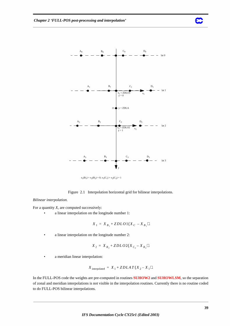
A 16 points horizontal grid is defined as is shown inFig. 2.1. The interpolation pointO is betweenB1, C1, B2 and
C2. and are the longitudes and latitudes on the computational sphere (departure geometry). The fo
weights are defined as follows:• zonal weight number 1:
• zonal weight number 2:
• meridian weight:
LdT dz⁄( )st
K m 1–
Ra
g
Λ Θ
ZDLO1ΛO ΛB1
–
ΛC1ΛB1
–------------------------=
ZDLO2ΛO ΛB2
–
ΛC2ΛB2
–------------------------=
ZDLATΘO ΘB1
–
ΘB2ΘB1
–-------------------------=
38
IFS Documentation Cycle CY25r1 (Edited 2003)
Chapter 2 ‘FULL-POS post-processing and interpolation’
oded
Figure 2.1 Interpolation horizontal grid for bilinear interpolations.
Bilinear interpolation.
For a quantityX, are computed successively:
• a linear interpolation on the longitude number 1:
.
• a linear interpolation on the longitude number 2:
.
• a meridian linear interpolation:
.
In the FULL-POS code the weights are pre-computed in routinesSUHOW2 andSUHOWLSM , so the separation
of zonal and meridian interpolations is not visible in the interpolation routines. Currently there is no routine c
to do FULL-POS bilinear interpolations.
A0 B0 C0 D0
A1 B1 C1 D1
A2 B2 C2 D2
A3 B3 C3 D3
lat 0
lat 1
lat 2
lat 3
O
x1 = ZDLO1y = 0
x2 = ZDLO2y = 1
y = ZDLA
x1
x2
y
x1(B1) = x2(B2) = 0; x1(C1) = x2(C2) = 1
X1 X B1ZDLO1 XC X B1
–( )+=
X2 X B2ZDLO2 XC2
X B2–( )+=
X interpolated X1 ZDLAT X2 X1–( )+=
39
IFS Documentation Cycle CY25r1 (Edited 2003)
Part VI: ‘Technical and computational procedures’
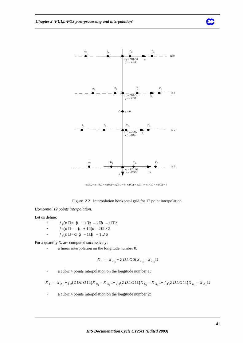
2.3.2 12 points horizontal interpolations.
Horizontal interpolation grid and weights for 12 points cubic interpolations.
A 16 points horizontal grid is defined as shown inFig. 2.2. The interpolation pointO is betweenB1, C1, B2 and
C2. The following weights are defined as follows:
• zonal weight number 0:
• zonal weight number 1:
• zonal weight number 2:
• zonal weight number 3:
• meridian weights:
ZDLO0ΛO ΛB0
–
ΛC0ΛB0
–------------------------=
ZDLO1ΛO ΛB1
–
ΛC1ΛB1
–------------------------=
ZDLO2ΛO ΛB2
–
ΛC2ΛB2
–------------------------=
ZDLO3ΛO ΛB3
–
ΛC3ΛB3
–------------------------=
ZCLA2ΘO ΘB0
–( ) ΘO ΘB2–( ) ΘO ΘB3
–( )ΘB1
ΘB0–( ) ΘB1
ΘB2–( ) ΘB1
ΘB3–( )
------------------------------------------------------------------------------------------=
ZCLA3ΘO ΘB0
–( ) ΘO ΘB1–( ) ΘO ΘB3
–( )ΘB2
ΘB0–( ) ΘB2
ΘB1–( ) ΘB2
ΘB3–( )
------------------------------------------------------------------------------------------=
ZCLA4ΘO ΘB0
–( ) ΘO ΘB1–( ) ΘO ΘB2
–( )ΘB3
ΘB0–( ) ΘB3
ΘB1–( ) ΘB3
ΘB2–( )
------------------------------------------------------------------------------------------=
40
IFS Documentation Cycle CY25r1 (Edited 2003)
Chapter 2 ‘FULL-POS post-processing and interpolation’
Figure 2.2 Interpolation horizontal grid for 12 point interpolation.
Horizontal 12 points interpolation.
Let us define:
•
•
•
For a quantityX, are computed successively:
• a linear interpolation on the longitude number 0:
.
• a cubic 4 points interpolation on the longitude number 1:
.
• a cubic 4 points interpolation on the longitude number 2:
A0 B0 C0 D0
A1 B1 C1 D1
A2 B2 C2 D2
A3 B3 C3 D3
lat 0
lat 1
lat 2
lat 3
O
x1 = ZDLO1y = - ZDB
x2 = ZDLO2y = - ZDC
y = 0
x1
x2
y
x0(B0) = x1(B1) = x2(B2) = x3(B3) = 0; x0(C0) = x1(C1) = x2(C2) = x3(C3) = 1
x0
x3
x0 = ZDLO0y = - ZDA
x3 = ZDLO3y = - ZDD
f 2 α( ) α 1+( ) α 2–( ) α 1–( ) 2⁄=
f 3 α( ) α 1+( )– α 2–( )α 2⁄=
f 4 α( ) α α 1–( ) α 1+( ) 6⁄=
X0 X B0ZDLO0 XC0
X B0–( )+=
X1 X A1f 2 ZDLO1( ) X B1
X A1–( ) f 3 ZDLO1( ) XC1
X A1–( ) f 4 ZDLO1( ) X D1
X A1–( )+ + +=
41
IFS Documentation Cycle CY25r1 (Edited 2003)
Part VI: ‘Technical and computational procedures’
the
o be
d for
ted in
tine
d the
.
mber
an be
ed
en the
trapola-
.
• a linear interpolation on the longitude number 3:
.
• a meridian cubic 4 points interpolation:
.
In the FULL-POS code the weights are pre-computed in routinesSUHOW2 andSUHOWLSM , so the separation
of zonal and meridian interpolations is not visible in the interpolation routines.
2.3.3 Location of computations.
Once the coordinates of the interpolation points known:
• The “north-western" model grid point coordinates are computed in the routineSUHOW1. This is
the model (departure geometry) grid point which is immediately at the north-west of
interpolation point.
• The weights not modified by the land-sea mask are computed in routineSUHOW1.
• The weights modified by the land-sea mask are computed in routineSUHOWLSM . This is
equivalent to use weights not modified by the land-sea mask and to multiply the field t
interpolated by the land-sea mask (0 if sea, 1 if land).
• The horizontal 12 points interpolations are done by routinesFPAERO (variables linked to
aeronautic jet),FPHOR12 (3D derivatives) andFPINT12 (other variables). RoutineFPMIMAXis used to give to the interpolated quantity the value of the nearest model grid point (use
maximum and minimum temperature at 2 meters). They need intermediate quantities compu
routineFPSCAW.
•
Additional modifications can be done in the interpolation routines after interpolations (principally in rou
FPINT12), for example add a monotonicity condition. More details about these additional modifications an
post-processed fields concerned by these modifications are described in the part describing each routine
2.3.4 Plane geometry (ALADIN).
All previous formulae for weight computation can be used for an irregular latitude spacing and a different nu
of points on each longitude. The ALADIN grid has a horizontal regular spacing, so the previous formulae c
simplified. SUEHOW1, SUEHOW2 and SUEHOWLSM are called instead ofSUHOW1, SUHOW2 and
SUHOWLSM . SUEHOW1, SUEHOW2 andSUEHOWLSM are currently not yet coded and have to be cod
in the future cycle AL09 based on the future cycle 18T1 of ARPEGE/IFS.
2.4 VERTICAL INTERPOLATIONS AND EXTRAPOLATIONS .
2.4.1 General considerations.
For 3D variables to be vertically interpolated, vertical interpolations are generally linear interpolations betwe
layers where are defined model variables. The treatment of the extrapolations above the upper layer, the ex
X2 X A2f 2 ZDLO2( ) X B2
X A2–( ) f 3 ZDLO2( ) XC2
X A2–( ) f 4 ZDLO2( ) X D2
X A2–( )+ + +=
X3 X B3ZDLO3 XC3
X B3–( )+=
X interpolated X0 ZCLA2 X1 X0–( ) ZCLA3 X2 X0–( ) ZCLA4 X3 X0–( )+ + +=
42
IFS Documentation Cycle CY25r1 (Edited 2003)
Chapter 2 ‘FULL-POS post-processing and interpolation’
bles can
and 3.
and 2;
.
antity
.
e rou-
f the
ct that
in this
about
m of
een
tions below the lower layer or the surface depend on the variable considered. In particular cases some varia
be diagnosed using the vertically interpolated value of some other variables.
The ‘OLD ’ versions of routines when available are used at ECMWF (switchLOLDPP=.T.). METEO-FRANCE
uses the optionLOLDPP=.F. .
2.4.2 More details for 3D dynamical variables.
Wind components, wind velocity.
Way of interpolating ifLOLDPP=.T. (routinePPUV_OLD):
• Linear interpolation between the layer 2 and the lower layer.
• The coordinate used for linear interpolation is the logarithm of the pressure.
• Quadratic interpolation between the layer 1 and the layer 2 using the values of the layers 1, 2
• Quadratic interpolation between the top and the layer 1 using the values of the top, layers 1
the value of the top is obtained by a linear extrapolation from the values of the layers 1 and 2
• The coordinate used for quadratic interpolation is the logarithm of the pressure.
• Extrapolation below the middle of the lower layer and below the surface assumes that the qu
is constant.
Way of interpolating ifLOLDPP=.F. (routinePPUV):
• The same as forLOLDPP=.T. but quadratic interpolations are replaced by linear interpolations
Temperature.
Applies to temperature if the vertical coordinate of post-processing is not the potential vorticity, otherwise se
tinePP2DINT.
Way of interpolating ifLOLDPP=.F. (routinePPT):
• Quadratic interpolation between the middles of the upper and lower layers.
• Quadratic interpolation between the top and the middle of the upper layer: the top value o
temperature is assumed to be equal to the value of the middle of the upper layer; due to the fa
the interpolation is a quadratic one, that does not mean that the temperature is constant
atmosphere depth.
• The coordinate used for quadratic interpolation is the logarithm of pressure. For more details
the quadratic interpolation used, which is a quadratic analytic expression of the logarith
pressure, and the reason of using a quadratic interpolation, see (Undén, 1995).
• A surface temperature \TSURF is computed as follows:
(2.1)
• Extrapolation below the middle of the lower layer and the surface is a linear interpolation betw
and .
• Extrapolation under the surface is made according a more complicated algorithm:
(2.2)
where:
Tsurf TLdTdz-------
stRa
g------
Πs
ΠL------- 1–
TL+=
TL Tsurf
Textrapolated Tsurf 1 y y2
2----- y3
6-----+ + +
=
43
IFS Documentation Cycle CY25r1 (Edited 2003)
Part VI: ‘Technical and computational procedures’
of
d
een
e rou-
ndard
f the
olation
onent
and 3.
and 2.
(2.3)
If ; if the expression for is more
complicated:
(2.4)
if :
(2.5)
• and : is computed by a linear interpolation (coordinate
interpolation is ) between the two values an
Way of interpolating ifLOLDPP=.T. (routinePPT_OLD):
• Linear interpolation (between the upper and the lower layer).
• The coordinate used for linear interpolation is the pressure.
• Extrapolation above the middle of the upper layer assumes that the quantity is constant.
• Extrapolation below the middle of the lower layer and the surface is a linear interpolation betw
TL and \TSURF like inPPT.
• Extrapolation under the surface is made according the same algorithm as inPPT (code of part 1.4 is
different inPPT and inPPT_OLD but actually does the same calculations).
Geopotential.
Applies to geopotential if the vertical coordinate of post-processing is not the potential vorticity, otherwise se
tinePP2DINT.
Way of interpolating ifLOLDPP=.T. (routinePPGEOP_OLD):
• The variable interpolated is a geopotential departure from a reference defined by a sta
atmosphere without any orography. After the interpolation an increment is added, sum o
surface orography and the ‘standard’ geopotential depth between the pressure level of interp
and the actual surface. This method avoids to introduce interpolations for the standard comp
of the geopotential which can be computed analytically (in routinePPSTA).
• Linear interpolation between the layer 2 and the surface.
• The coordinate used for linear interpolation is the logarithm of the pressure.
• Quadratic interpolation between the layer 1 and the layer 2 using the values of the layers 1, 2
• Quadratic interpolation between the top and the layer 1 using the values of the top, layers 1
• The coordinate used for quadratic interpolation is the logarithm of the pressure.
• Extrapolation below surface uses the surface temperatur ofEq. (2.1).
(2.6)
• where is defined by formula(2.3) with in all cases.
y ΓRa
g------
Πs
ΠL-------
log=
Φs g 2000 m,<⁄ Γ dT dz⁄( )st= Φs g 2000 m,≥⁄ Γ
Γ gΦs------max T0′ Tsurf 0,–( )=
Φs g 2500 m,>⁄
T0′ min TsurfdTdz-------
stΦs
g------ 298 K,+
=
Φs g 2500 m≤⁄ Φs g 2000 m,≥⁄ T0′Φs min Tsurf dT dz⁄( )st Φs g⁄( ) 298 K,+( )
Tsurf dT dz⁄( )st Φs g⁄( )+
Tsurf
Φextrapolated Φs RaTsurf
Πs
ΠL-------
1 y2--- y2
6-----+ +
log–=
y Γ dT( ) dz( )⁄( )st=
44
IFS Documentation Cycle CY25r1 (Edited 2003)
Chapter 2 ‘FULL-POS post-processing and interpolation’
ndard
f the
olation
onent
ratic
e
re for
ing a
le of
antity
• For more details about this algorithm, see (Anderssonand Courtier, 1992) which is still valid for the
cycles 17 and 18.
Way of interpolating ifLOLDPP=.F. (routinePPGEOP):
• The variable interpolated is a geopotential departure from a reference defined by a sta
atmosphere without any orography. After the interpolation an increment is added, sum o
surface orography and the “standard" geopotential depth between the pressure level of interp
and the actual surface. This method avoids to introduce interpolations for the standard comp
of the geopotential which can be computed analytically (in routinePPSTA).
• Quadratic interpolation between the middles of the upper and lower layers.
• Quadratic interpolation between the top and the middle of the upper layer.
• The coordinate used for quadratic interpolation is the logarithm of pressure. The quad
interpolation is not exactly the same as forLOLDPP=.T., it is a quadratic analytic expression of th
logarithm of pressure of the same type as the one used to post-process the temperatu
LOLDPP=.F. . For more details about the quadratic interpolation used, and the reason of us
quadratic interpolation, see (Undén, 1995).
• Linear interpolation between the lower layer and the surface, as forLOLDPP=.T. .
• Extrapolation below surface uses the same algorithm as forLOLDPP=.T. .
2.4.2 (a) Variables interpolated using routine PP2DINT.
List of variables:
• Geopotential if vertical coordinate is potential vorticity.
• Temperature if vertical coordinate is potential vorticity.
• Relative vorticity .
• Divergence .
• Potential temperature if vertical coordinate is not potential temperature.
• Velocity potential .
• Stream function .
• Equivalent potential temperature .
• Absolute vorticity .
• Stretching deformation .
• Shearing deformation .
• Potential vorticity .
• Wet potential vorticity (not yet coded).
Way of interpolating:
• Linear interpolation (between the upper and the lower layer for quantities defined on the midd
layers, between the layer 1 and the surface for quantities defined on interlayers).
• The coordinate used for linear interpolation is the pressure.
• Extrapolation above the middle of the upper layer assumes that the quantity is constant.
• Extrapolation below the middle of the lower layer and below the surface assumes that the qu
is constant.
Moisture, liquid water, solid water, cloud fraction, passive scalars: variables using routine PPQ.
Way of interpolating (routinePPQ):
• Linear interpolation (between the upper and the lower layer).
• The coordinate used for linear interpolation is the pressure.
• Extrapolation above the middle of the upper layer assumes that the quantity is constant.
ΦT
ζD
Θψ
χΘe
ζ f+
STDSHD
PVPVw
45
IFS Documentation Cycle CY25r1 (Edited 2003)
Part VI: ‘Technical and computational procedures’
antity
antity
lue at
tity is
, mois-
compli-
ses one
ing
• Extrapolation below the middle of the lower layer and below the surface assumes that the qu
is constant.
Relative humidity (routine PPRH).
Way of interpolating (routinePPRH):
• Linear interpolation (between the upper and the lower layer).
• The coordinate used for linear interpolation is the pressure.
• Extrapolation above the middle of the upper layer assumes that the quantity is constant.
• Extrapolation below the middle of the lower layer and below the surface assumes that the qu
is constant.
Pressure coordinate vertical velocity (routine PPVVEL).
Way of interpolating (routinePPVVEL ):
• Linear interpolation (between the upper and the lower layer).
• The coordinate used for linear interpolation is the pressure.
• Extrapolation above the middle of the upper layer is a linear interpolation between a zero va
the top and the value of the upper layer.
• Extrapolation between the middle of the lower layer and the surface assumes that the quan
constant.
• Extrapolation below the surface assumes that the quantity is zero.
Moist (irreversible) pseudo-adiabatic potential temperature (routine PPTHPW.
RoutinePPTHPW is a diagnostic one. It takes as input the vertically post-processed pressure, temperature
ture, liquid water and ice and computes at the post-processing levels using a diagnostic (and rather
cated) algorithm.
2.4.3 2D dynamical variables which need extrapolations.
Mean sea level pressure (routine PPPMER).
If is lower than 0.001 the mean sea level pressure is set to the surface pressure. In the other ca
uses the following algorithm:
• One computes the surface temperature ofEq. (2.1) and the ‘mean sea level’ temperature
.
• To avoid extrapolation of too low pressures over high and warm surfaces the follow
modifications are done:
• if and , is defined by:
(2.7)
• if and , is set to 0, is modified and set to
.
ω
Θ′w
Θ′w
ΠMSL
Φs J kg 1–
Tsurf
T0 TsurfdTdz-------
stΦs
g------+=
T0 290.5 K> Tsurf 290.5 K≤ Γ
Γ 290.5 Tsurf–( ) gΦs------=
T0 290.5 K> Tsurf 290.5 K> Γ Tsurf
0.5 255 K old value ofTsurf+( )×
46
IFS Documentation Cycle CY25r1 (Edited 2003)
Chapter 2 ‘FULL-POS post-processing and interpolation’
done
o
city,
dinate
ical
ring
the for-
• To avoid extrapolation of too high pressures over cold surfaces the following modifications are
when : is set to and is modified and set t
.
• In the other cases is set to .
• Mean sea level pressure is computed as follows:
(2.8)
where:
(2.9)
2.5 FILTERING IN SPECTRAL SPACE .
2.5.1 General considerations.
Three filterings are successively applied:
• 1) A “THX" filter on derivatives in ARPEGE, or a bell-shaped filter on derivatives for ALADIN.
• 2) A bell-shaped filter on all fields (derivatives and not derivatives).
• 3) A “THX" filter on all fields.
Filtering is done in routinepp_obs/SPOS (pp_obs/ESPOS for ALADIN).
2.5.2 ‘THX’ (ARPEGE) or bell-shaped (ALADIN) filtering on derivatives.
Cases where this filtering is used:
This filtering applies in the spectral space to absolute vorticity, relative vorticity, divergence, vertical velo
stretching and shearing deformations, and potential vorticity (and extend to all variables if the vertical coor
of post-processing is the potential vorticity). This filter is active if:
• CFPFMT is not ‘MODEL’ in namelistNAMFPC .
• LFPFIL =.TRUE. in namelist NAMFPF for ARPEGE, or LFPBED=.TRUE. in namelist
NAMFPF for ALADIN.
• VariableNFMAX is smaller than the ‘equivalent unstretched sphere’ truncation (in pract
is between and , where is the stretching factor.
If you wish to keep these fields unfiltered, then just setLFPFIL =.FALSE. in ARPEGE/IFS, orLFPBED=.FALSE.
in ALADIN (namelist NAMFPF ). On the other hand, you can keep the filter active but you can tune the filte
function.
Function of filtering:
In ARPEGE/IFS, this function looks like a smoothed step function; for a given total wavenumbern in the un-
stretched spectral space (i.e. the spectral space of the ‘equivalent unstretched sphere’ of truncation ),
mula is:
Tsurf 255 K< Γ dT dz⁄( )st Tsurf
0.5 255 K old value of+ Tsurf( )×Γ dT dz⁄( )st
ΠMSL Πs
Φs
RaTsurf------------------ 1 x
2---– x2
3-----+
exp=
xΓΦs
gTsurf---------------=
Nc
Nc 1.1 c Ns×× 1.2 c Ns×× c
Nc
47
IFS Documentation Cycle CY25r1 (Edited 2003)
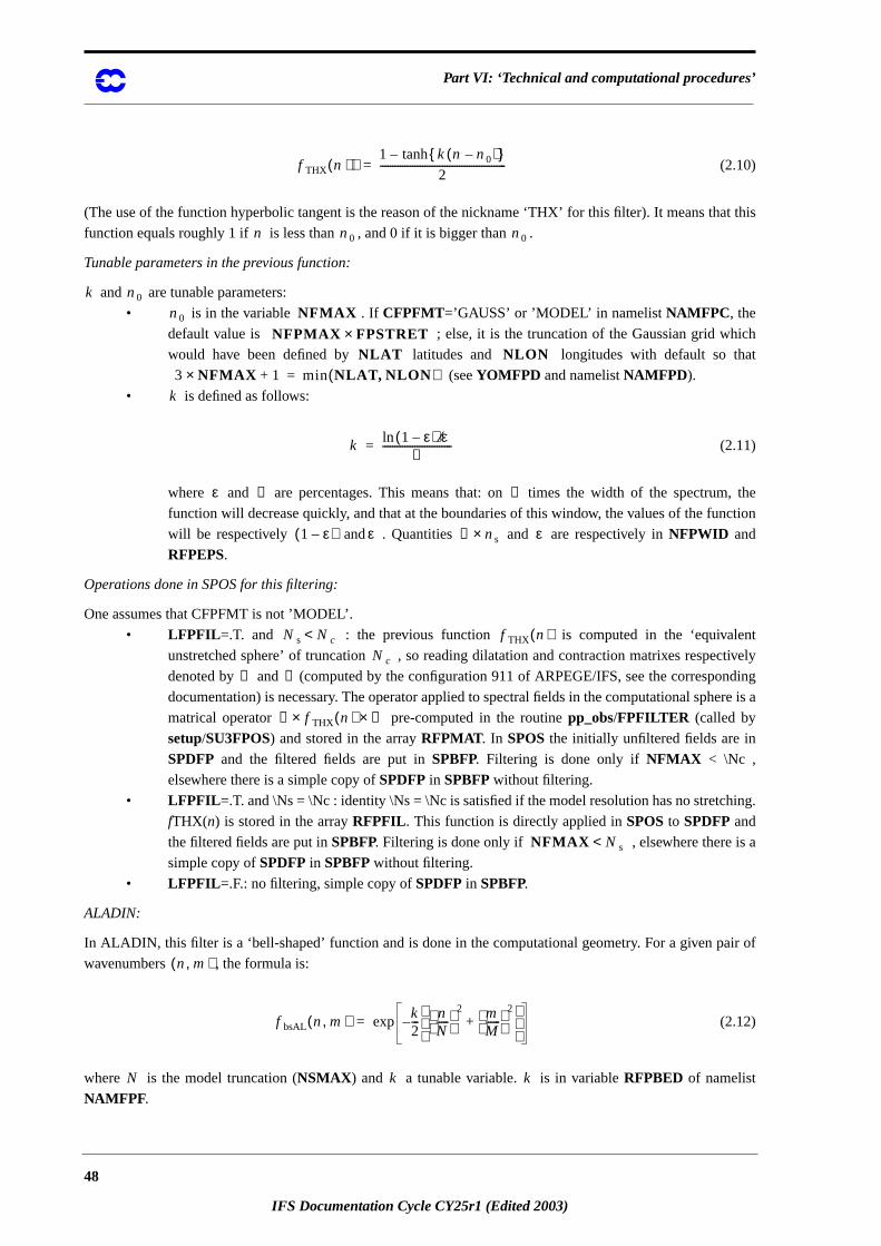
Part VI: ‘Technical and computational procedures’
t this
ich
that
, the
ction
nt
tively
nding
ere is a
ing.
a
ir of
(2.10)
(The use of the function hyperbolic tangent is the reason of the nickname ‘THX’ for this filter). It means tha
function equals roughly 1 if is less than , and 0 if it is bigger than .
Tunable parameters in the previous function:
and are tunable parameters:
• is in the variable . IfCFPFMT=’GAUSS’ or ’MODEL’ in namelistNAMFPC , the
default value is ; else, it is the truncation of the Gaussian grid wh
would have been defined by latitudes and longitudes with default so
(seeYOMFPD and namelistNAMFPD ).
• is defined as follows:
(2.11)
where and are percentages. This means that: on times the width of the spectrum
function will decrease quickly, and that at the boundaries of this window, the values of the fun
will be respectively and . Quantities and are respectively inNFPWID and
RFPEPS.
Operations done in SPOS for this filtering:
One assumes that CFPFMT is not ’MODEL’.
• LFPFIL =.T. and : the previous function is computed in the ‘equivale
unstretched sphere’ of truncation , so reading dilatation and contraction matrixes respec
denoted by and (computed by the configuration 911 of ARPEGE/IFS, see the correspo
documentation) is necessary. The operator applied to spectral fields in the computational sph
matrical operator pre-computed in the routinepp_obs/FPFILTER (called by
setup/SU3FPOS) and stored in the arrayRFPMAT . In SPOSthe initially unfiltered fields are in
SPDFP and the filtered fields are put inSPBFP. Filtering is done only ifNFMAX < \Nc ,
elsewhere there is a simple copy ofSPDFP in SPBFP without filtering.
• LFPFIL =.T. and \Ns = \Nc : identity \Ns = \Nc is satisfied if the model resolution has no stretch
fTHX(n) is stored in the arrayRFPFIL . This function is directly applied inSPOSto SPDFPand
the filtered fields are put inSPBFP. Filtering is done only if , elsewhere there is
simple copy ofSPDFP in SPBFP without filtering.
• LFPFIL =.F.: no filtering, simple copy ofSPDFP in SPBFP.
ALADIN:
In ALADIN, this filter is a ‘bell-shaped’ function and is done in the computational geometry. For a given pa
wavenumbers , the formula is:
(2.12)
where is the model truncation (NSMAX ) and a tunable variable. is in variableRFPBED of namelist
NAMFPF.
f THX n )( )1 k n n0–( ){ }tanh–
2---------------------------------------------------=
n n0 n0
k n0
n0 NFMAXNFPMAX FPSTRET×
NLAT NLON3 NFMAX 1+× min NLAT NLON,( )=
k
k 1 ε–( ) ε⁄lnL
----------------------------=
ε L L
1 ε–( ) ε L ns× ε
Ns Nc< f THX n( )Nc
D C
C f THX n( ) D××
NFMAX Ns<
n m,( )
f bsAL n m,( ) k2--- n
N-----
2 mM------
2
+
–exp=
N k k
48
IFS Documentation Cycle CY25r1 (Edited 2003)
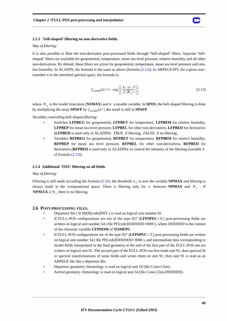
Chapter 2 ‘FULL-POS post-processing and interpolation’
‘bell-
ll other
nd rela-
nt
g to
are
ral fit
as an
2.5.3 ‘Bell-shaped’ filtering on non-derivative fields.
Way of filtering:
It is also possible to filter the non-derivative post-processed fields through “bell-shaped" filters. Separate
shaped’ filters are available for geopotential, temperature, mean sea level pressure, relative humidity and a
non-derivatives. By default, these filters are active for geopotential, temperature, mean sea level pressure a
tive humidity. In ALADIN, the formula is the same as above (formula(2.12)). In ARPEGE/IFS, for a given wav-
enumbern in the stretched spectral space, the formula is:
(2.13)
where is the model truncation (NSMAX ) and a tunable variable. InSPOS, the bell-shaped filtering is done
by multiplying the arraySPAFP by , the result is still inSPAFP.
Variables controlling bell-shaped filtering:
• SwitchesLFPBEG for geopotential,LFPBET for temperature,LFPBEH for relative humidity,
LFPBEP for mean sea level pressure,LFPBEL for other non-derivatives,LFPBED for derivatives
(LFPBED is used only in ALADIN): .TRUE. if filtering, .FALSE. if no filtering.
• VariablesRFPBEG for geopotential,RFPBET for temperature,RFPBEH for relative humidity,
RFPBEP for mean sea level pressure,RFPBEL for other non-derivatives,RFPBED for
derivatives (RFPBED is used only in ALADIN): to control the intensity of the filtering (variable
of formula(2.13)).
2.5.4 Additional ‘THX’ filtering on all fields.
Way of filtering:
Filtering is still made according the formula(2.10): the threshold is now the variableNPMAX and filtering is
always made in the computational space. There is filtering only for betweenNPMAX and . If
there is no filtering.
2.6 POST-PROCESSING FILES.• Departure file ( ICMSH[code]INIT ) is read on logical unit number 81.
• If FULL-POS configurations are not of the type 927 (LFPSPEC=.F.) post-processing fields are
written on logical unit number 54 ( file PF[code]DDDDDD+0000 ), where DDDDDD is the conte
of the character variableCFPDOM of YOMFPC .
• If FULL-POS configurations are of the type 927 (LFPSPEC=.T.) post-processing fields are written
on logical unit number 54 ( file PF[code]DDDDDD+0000 ), and intermediate data correspondin
model fields interpolated in the final geometry at the end of the first part of the FULL-POS run
written on logical unit 91. The second part of the FULL-POS run first reads unit 91, does spect
or spectral transformations of some fields and writes them on unit 91; then unit 91 is read
ARPEGE file like a departure file.
• Departure geometry climatology is read on logical unit 10 (file Const.Clim).
• Arrival geometry climatology is read on logical unit 54 (file Const.Clim.DDDDDD).
f bsARP n( ) k2--- n
Ns-------
2–
exp=
Ns kf bsARP n( )
k
n0
n Ns
NPMAX Ns≥
49
IFS Documentation Cycle CY25r1 (Edited 2003)
Part VI: ‘Technical and computational procedures’
2.7 ORGANIGRAM
When not precised, directory ispp_obs (except forLFI... routines which are in the auxiliary library).
Routines ending bySM (ex. SPECFITASM, SPECFITGSM, SCAN2MSM, SPEREESM, REESPESM,
UVSPESM, SPECRTSM ) are written as they are in cycle 18. The suffixSM disappears in cycle 17.
2.7.1 Setup routines and arborescence above STEPO.
General architecture under CNT0:
Only features concerning FULL-POS are mentioned.
control/CNT0• setup/SU0YOMA
• setup/SUCT0• setup/SUAFN
• setup/SUAFN1• setup/SUAFN2
• setup/SUFPC• setup/SUDIM setup/SUFPDIM
• setup/SUFPDYN setup/SUFPDOM• setup/SUFPCONF• transform /UPDVPOS setup/SUVPOS• setup/SUFPFIT• pp_obs/CPVPOSPR
• setup/SUFPD utility /EGGX• utility /EGGRVS• ALADIN routine EGGMLT
• setup/SUCFU setup/SUCFUFP• setup/SUXFU setup/SUXFUFP• setup/SUGPPRP pp_obs/FPINIPHY• setup/SUAFPOS
• setup/SURFPDS• setup/SUWFPDS• setup/SUAFPDS
• setup/SUALLO setup/SUALFPOS• setup/SU0YOMB
• setup/SUMP• setup/SUALMP2• some other routines which do not contain any FULL-POS feature.
• setup/SUFPG• setup/SUFPG1
• setup/DFLTVV1• setup/SUGAW (arborescence is not described in detail).
• setup/SUNMEN• setup/SUFPG2
• utility /EGGX utility /EGGRVS and ALADIN routineEGGMLT• transform /TRACARE
→→
→
→ →→
→
→ →
→→
→→
→→
→
→→
→→
50
IFS Documentation Cycle CY25r1 (Edited 2003)
Chapter 2 ‘FULL-POS post-processing and interpolation’
• setup/SUGENORD• utility /EGGDIR• utility /EGGRVS• transform /TRARECA
• setup/SUSC2• setup/SUSIZBUF• ARPEGE: setup/SUFPCSET setup/SUFPRSET processor
communication routinesMPE_SEND andMPE_RECV.
• Some multitasking routines.
• Some transposition routines (do not touch FULL-POS).
• SomeMIO... routines (do not touch FULL-POS).
• setup/SUBFPOS• setup/SUFPF• setup/SUFPOPH setup/SUFRAME FACADE (or SUEFRAME if
plane geometry, orSUFPGRIB if GRIB files).
• setup/SUFPSC2• setup/SUFPIOS MIOOPEN• setup/SUFPSC2B
• control/CNT1 (see below arborescence underCNT1).
General architecture under CNT1:
Only features concerning FULL-POS are mentioned. For arborescence undertransform /REESPESM, trans-form /SPEREESM, transform /UVSPESM see documentation about spectral transforms.control/CNT1
• setup/SU1YOM• setup/SUINIF
• pp_obs/SPECFITASM• utility /CHIEN (or the ALADIN routineCCHIEN if ALADIN).
• LFI... andFA... routines.
• transform /REESPESM (ARPEGE) ortransform /EREESPE (ALADIN)
• transform /SPEREESM (ARPEGE) ortransform /ESPEREE (ALADIN)
• transform /UVSPESM• pp_obs/SPECFITADM
• utility /CHIEN or utility /CCHIEN• LFI... andFA... routines.
• processor communication routines parallel/DISGRID , parallel/DIWRGRID , parallel/DIWRSPE, parallel/FPDISPVECTOR, which call
MPE_SEND andMPE_RECV.
• transform /REESPESM (ARPEGE) or transform /EREESPEDM(ALADIN)
• transform /SPEREESM (ARPEGE) or transform /ESPEREEDM(ALADIN)
• transform /UVSPESM• pp_obs/SPECFITGSM (GRIB version of SPECFITASM, arborescence not
detailed)
• pp_obs/SPECFITGDM (GRIB version of SPECFITADM , arborescence not
detailed)
→
→ →
→ →
→
→
→→
→→
→
51
IFS Documentation Cycle CY25r1 (Edited 2003)
Part VI: ‘Technical and computational procedures’
• setup/SUSPEC, setup/SUGRIDF, setup/SUGRIDU, adiab/SPECRTSM, adiab/
SPECRTDM, setup/SUGRCFU, setup/SUGRXFU (arborescence not detailed)
• other routines without any relationship with FULL-POS.
• control/CNT2 control/CNT3 (see below arborescence underCNT3).
General architecture under CNT3:
Only features concerning FULL-POS are mentioned.control/CNT3• setup/SU3FPOS
• ARPEGE:setup/SUHOW1• setup/SURFPBUF
• pp_obs/CPCLIMO• ARPEGE:setup/SUHOW2• pp_obs/FPSCAW• utility /SC2RDG utility /EMPTB and “MIO" routines.
• parallel/FPADD3P (DM)
• parallel/FPWRIT (DM) processor communication routine
MPE_SEND.
• parallel/FPREAD (DM) processor communication routine
MPE_RECV.
• parallel/FPEXTPOL (DM)
• adiab/EXTMERB (no DM)
• adiab/INIPEX (no DM)
• adiab/EXTPOLB (no DM)
• pp_obs/FPINT12• “MIO" routines.
• c9xx/RDCLIMO utility /CHIEN , “LFI" end “FA" routines.
• c9xx/RDECCLIMO (GRIB version ofRDCLIMO ) GRIB routines.
• utility /SC2WRG utility /FILLB• processor communication routinesparallel/FPSENDTOPROC1, parallel/
FPDISPTOPROC1, which callMPE_SENDandMPE_RECV for cycle 17 (do not
work properly).
• processor communication routinesparallel/OSNDGPFFP, parallel/ORCVGPFFP,
parallel/ISNDGPFFP, parallel/IRCVGPFFP, which call MPE_SEND and
MPE_RECV; processor communication routineMPE_BARRIER for cycle 18.
• setup/SUWFPBUF• pp_obs/CPCLIMI
• pp_obs/FPSCAW• utility /SC2RDG utility /EMPTB and “MIO" routines.
• parallel/FPADD3P (DM)
• parallel/FPWRIT (DM) processor communication routine
MPE_SEND.
• parallel/FPREAD (DM) processor communication routine
MPE_RECV.
• parallel/FPEXTPOL (DM)
• adiab/EXTMERB (no DM)
• adiab/INIPEX (no DM)
• adiab/EXTPOLB (no DM)
→ →
→→
→→
→
→
→
→→
→
→→
→
→
→
52
IFS Documentation Cycle CY25r1 (Edited 2003)
Chapter 2 ‘FULL-POS post-processing and interpolation’
e
• “MIO" routines.
• pp_obs/CPCLIMO• ARPEGE:setup/SUHOW2• pp_obs/FPSCAW• utility /SC2RDG utility /EMPTB and “MIO" routines.
• parallel/FPADD3P (DM)
• parallel/FPWRIT (DM) processor communication routine
MPE_SEND.
• parallel/FPREAD (DM) processor communication routine
MPE_RECV.
• parallel/FPEXTPOL (DM)
• adiab/EXTMERB (no DM)
• adiab/INIPEX (no DM)
• adiab/EXTPOLB (no DM)
• pp_obs/FPINT12• “MIO" routines.
• utility /EXTGPF (utility /SC2RDG utility /EMPTB ) and “MIO"
routines.
• c9xx/RDCLIMO utility /CHIEN , “LFI" end “FA" routines.
• c9xx/RDECCLIMO (GRIB version ofRDCLIMO ) GRIB routines.
• processor communication routineparallel/FPDISPTOPROC1, which calls
MPE_SEND andMPE_RECV for cycle 17 (do not work properly).
• processor communication routinesparallel/ISNDGPFFP, parallel/IRCVGPFFP,
which call MPE_SEND and MPE_RECV; processor communication routine
MPE_BARRIER for cycle 18.
• ARPEGE:setup/SUHOW2• ARPEGE:setup/SUHOWLSM• “MIO" routines.
• utility /SC2WRG utility /FILLB• pp_obs/FPFILTER
• control/CNT4 (see below arborescence underCNT4).
• setup/SU4FPOS• pp_obs/PPREQ• setup/SUFPPHY setup/SUFPDOM• setup/SUFPDYN setup/SUFPDOM
• control/CPREP4 (see below arborescence underCPREP4).
Remark:SU4FPOSandCPREP4are also called byvar/ARCHFP when using FULL-POS mode 927 to truncat
the trajectory from high resolution to low resolution.
General architecture under CNT4:
Only features concerning FULL-POS are mentioned.control/CNT4• setup/SU4FPOS
• pp_obs/PPREQ• setup/SUFPPHY setup/SUFPDOM• setup/SUFPDYN setup/SUFPDOM
• pp_obs/GRIDFPOS (see below arborescence underGRIDFPOS).
→
→
→
→
→ →
→→
→
→→
→→
→
→→
→→
→
53
IFS Documentation Cycle CY25r1 (Edited 2003)
Part VI: ‘Technical and computational procedures’
• pp_obs/DYNFPOS (see below arborescence underDYNFPOS).
• control/CPREP4 (see below arborescence underCPREP4).
General architecture under GRIDFPOS:
Only features concerning FULL-POS are mentioned.pp_obs/GRIDFPOS• utility /CPGRIDF
• utility /SC2RDG utility /EMPTB• utility /SC2WRG utility /FILLB• some “MIO" routines.
• utility /PKGRIDA (or PKGRIDG if use of GRIB files, not described in detail)
• some “FA" and “LFI" routines.
• processor communication routines parallel/FPSENDTOPROC2, parallel/FPDISPTOPROC2, which callMPE_SEND andMPE_RECV (do not work properly).
• utility /SC2RDG utility /EMPTB• utility /SC2WRG utility /FILLB• utility /EXTGPF (no DM) (utility /SC2RDG utility /EMPTB ) and “MIO"
routines.
• utility /INCGPF (no DM)
• utility /SC2RDG utility /EMPTB• utility /SC2WRG utility /FILLB• some “MIO" routines.
• pp_obs/FPMODCFU pp_obs/FPMODPREC• utility /SC2RDG utility /EMPTB• utility /SC2WRG utility /FILLB• utility /EXTGPF (no DM) (utility /SC2RDG utility /EMPTB ) and “MIO"
routines.
• utility /INCGPF (no DM)
• utility /SC2RDG utility /EMPTB• utility /SC2WRG utility /FILLB• some “MIO" routines.
• parallel/FPADD3P (DM)
• parallel/FPREAD (DM) processor communication routineMPE_RECV.
• parallel/FPWRIT (DM) processor communication routineMPE_SEND.
• parallel/FPEXTPOL (DM)
• adiab/EXTMERB (no DM)
• adiab/INIPEX (no DM)
• adiab/EXTPOLB (no DM)
• pp_obs/FPSCAW2• pp_obs/FPOLIS• some “MIO" routines.
• pp_obs/FPMODXFU pp_obs/FPMODPREC• utility /SC2RDG utility /EMPTB• utility /SC2WRG utility /FILLB• utility /EXTGPF (no DM) (utility /SC2RDG utility /EMPTB ) and “MIO"
routines.
• utility /INCGPF (no DM)
• utility /SC2RDG utility /EMPTB
→→
→→
→→
→
→→
→ →
→→→
→ →→→
→ →
→→→
→→
→ →→→
→ →
→→
54
IFS Documentation Cycle CY25r1 (Edited 2003)
Chapter 2 ‘FULL-POS post-processing and interpolation’
.
• utility /SC2WRG utility /FILLB• some “MIO" routines.
• parallel/FPADD3P (DM)
• parallel/FPREAD (DM) processor communication routineMPE_RECV.
• parallel/FPWRIT (DM) processor communication routineMPE_SEND.
• parallel/FPEXTPOL (DM)
• adiab/EXTMERB (no DM)
• adiab/INIPEX (no DM)
• adiab/EXTPOLB (no DM)
• pp_obs/FPSCAW2• pp_obs/FPOLIS• some “MIO" routines.
• utility /MAXGPFV• processor communication routines parallel/FPSENDTOPROC2, parallel/
FPDISPVECTOR, which callMPE_SEND andMPE_RECV for cycle 17 (do not work
properly).
• processor communication routinesparallel/OSNDGPF, parallel/ORCVGPF which call
MPE_SEND and MPE_RECV; processor communication routinesMPE_SEND,
MPE_RECV andMPE_BARRIER for cycle 18.
• utility /SC2RDG utility /EMPTB• utility /EXTGPF (no DM) (utility /SC2RDG utility /EMPTB ) and “MIO"
routines.
• control/SCAN2H control/SCAN2MSM (SM) or control/SCAN2MDM (DM) (see
below arborescence underCPREP4).• dia/WRHFP (WRMLFPL or WRMLFP if use of GRIB files, not described in detail)
• some “FA" and “LFI" routines.
• utility /EXTFPF (utility /SC2RDG utility /EMPTB ) and “MIO" routines.
• processor communication routinesparallel/FPSENDTOPROC1, which callsMPE_SENDandMPE_RECV (does not work properly).
• pp_obs/FPBIPER library routinesESPLIN, ESMOOTH andESHFT.
• dia/FPNORM
General architecture under DYNFPOS:
Only features concerning FULL-POS are mentioned.
pp_obs/DYNFPOS• setup/SUFPCONF• setup/SUVFPOS
• transform /UPDVPOS setup/SUVPOS• setup/SUFPFIT• pp_obs/CPVPOSPR• setup/CPFPDS setup/FPFINDS setup/SUFPDS
• setup/SUVFPOSL• control/STEPO (see below arborescence underSTEPO).
General architecture under CPREP4:
Only features concerning FULL-POS are mentioned.CPREP4 is divided in two parts calling the same routines
→
→→
→
→→ →
→ →
→
→ →
→
→
→→
→ →
→
55
IFS Documentation Cycle CY25r1 (Edited 2003)
Part VI: ‘Technical and computational procedures’
control/CPREP4• control/STEPO (see below arborescence underSTEPO).
• pp_obs/GRIDFPOS (see above arborescence underGRIDFPOS).
• pp_obs/DYNFPOS (see above arborescence underDYNFPOS).
• utility /ENDIOS several “MIO" routines and library routineHPSHRINK• utility /MATCLOSE “LFI" routine LFIFER .
• utility /FREEMEM several utility /DEAL... routines (DEALLO , DEALFPOS,
DEALDDH , DEALCOS, DEALCTV , DEALGES, DEALCAN , DEALSPA, DEALSC2,
DEALSCR, DEALMOD , DEALNMI ) andutility /DEELLO for ALADIN.
• control/CNT0 (see above arborescence underCNT0).
General architecture under STEPO:
Only features concerning FULL-POS are mentioned.
control/STEPO• Gestion of IO:utility /IOPACK (see below arborescence underIOPACK ).
• Inverse Legendre transforms:transform /LTINVH• utility /CPGRIDF
• utility /SC2RDG utility /EMPTB• utility /SC2WRG utility /FILLB• some “MIO" routines.
• Inverse Fourier transforms + grid point computations + direct Fourier transforms:control/SCAN2H control/SCAN2MSM (SM) or control/SCAN2MDM (DM) : (see below
arborescence underSCAN2MSM/SCAN2MDM ).
• Direct Legendre transforms:transform /LTDIRH• Spectral computations:control/SPCH (see below).
General architecture under IOPACK:
Part 6 ofIOPACK concerns FULL-POS.
utility /IOPACK• dia/WRPLFP for GRIB files, not described in detail.
• dia/WRPVLFP for GRIB files, not described in detail.
• dia/WRTHLFP for GRIB files, not described in detail.
• dia/WRMLFP for GRIB files, not described in detail.
• dia/ESPFP (for ALADIN)
• dia/WRSFP• “LFI" and “FA" routines.
• processor communication routineparallel/DIWRSPE, parallel/FPSENDTOPROC2,which callMPE_SEND andMPE_RECV (do not properly work).
• dia/SPNORMBL for ARPEGE (arborescence not described in detail)
• dia/SPNORMAVE for ARPEGE (arborescence not described in detail)
• dia/ESPNORMBL for ALADIN (arborescence not described in detail)
• utility /SC2RDG utility /EMPTB• utility /EXTGPF (utility /SC2RDG utility /EMPTB ) and “MIO" routines.
• dia/WRSFPMIO• “LFI" and “FA" routines.
• dia/SPNORMBL (arborescence not described in detail)
→→
→→
→→→
→
→
→→→
→ →
→
→
→→ →
→
56
IFS Documentation Cycle CY25r1 (Edited 2003)
Chapter 2 ‘FULL-POS post-processing and interpolation’
out
out
een
een
ween
• dia/SPNORMAVE (arborescence not described in detail)
• transform /SPEREESM (arborescence not described in detail, see documentation ab
spectral transforms).
• transform /REESPESM (arborescence not described in detail, see documentation ab
spectral transforms).
• utility /EXTGPF (utility /SC2RDG utility /EMPTB ) and “MIO" routines.
• utility /FILLB• utility /WRSPBUF “MIO" routines.
• “MIO" routines.
• dia/WRHFP• some “FA" and “LFI" routines.
• processor communication routineparallel/FPSENDTOPROC1, which callsMPE_SENDandMPE_RECV.
• utility /EXTFPF (utility /SC2RDG utility /EMPTB ) and “MIO" routines.
• pp_obs/FPBIPER library routinesESPLIN, ESMOOTH andESHFT.
• dia/FPNORM
2.7.2 Grid-point computations.
General architecture of SCAN2MSM (shared memory) and SCAN2MDM (distributed memory):
control/SCAN2H control/SCAN2MSM (SM) orcontrol/SCAN2MDM (DM) :
• Inverse Fourier transforms:transform /FTINVH .
• Some memory transfers and pointer computations before grid-point computations.
• Comparison with observations (non-lagged part, then information communication betw
processors, then lagged part).
• Model grid-point computations (non-lagged part, then information communication betw
processors, then lagged part).
• Post-processing (grid-point part, see below for more details).
• Grid-point computations for analysis.
• Direct Fourier transforms:transform /FTDIRH .
General architecture concerning FULL-POS in SCAN2MSM and SCAN2MDM:
FULL-POS undercontrol/SCAN2MSM or control/SCAN2MDM includes:
• Vertical interpolations.VPOS• utility /SC2RDG utility /EMPTB• CPVPOSR• POS (see below).
• utility /SC2WRG utility /FILLB• GPOS adiab/GPPRE andCTSTAR.
• Non lagged part of horizontal interpolations.HPOS• Functionutility /MGETBUF• utility /SC2RDG utility /EMPTB• adiab/EXTMERB (no DM)
• adiab/INIPEX (no DM)
• adiab/EXTPOLB (no DM)
• For distributed memory, some routines doing halo constitution and communications bet
processors before performing interpolations underHPOSLAG.
→ →
→
→
→ →→
→ →
→→
→→
→→
→
57
IFS Documentation Cycle CY25r1 (Edited 2003)
Part VI: ‘Technical and computational procedures’
ontal
model
• parallel/FPADD3P• parallel/FPWRIT processor communication routineMPE_SEND.
• parallel/FPREAD processor communication routineMPE_RECV.
• parallel/FPEXTPOL• Lagged part of horizontal interpolations and some vertical interpolations made after horiz
interpolations.HPOSLAG• Functionutility /MFINDBUF• FPOSHOR (see below)
• Functionutility /MDONEBUF• Diagnostic of the post-processable variables which are computed from the post-processed
variables (height or -levels post-processing and change of horizontal geometry).ENDVPOS
• utility /SC2RDG utility /EMPTB• CPVPOSPR• ENDPOS
• Severaladiab/GP... routines:GPRCP, GPPREH, GPXYB, GPPREF, GPGEO,
GPRH, GPTET, GPEPT.
• PPTHPW• utility /SC2WRG utility /FILLB
Organigram of POS:
• Several adiab/GP... routines: GPRCP, GPPREH, GPXYB, GPPREF, GPGEO, GPPVO,
GPEPT.
• CTSTAR*** A series of routines computing intermediate quantities and weights for vertical interpolations.
• PPINITZ• PPZHLEV• PPPS PPINTZ andEXPBESU• PPLTP• PPLTETA• PPLETA adiab/GPPREH, adiab/GPXYB andadiab/GPPREF• PPINIT• PPFLEV
*** A series of interpolation routines.
• PPUV• PPUV_OLD PPINTP andPPITPQ• PPINTP• (PPITPQ) (currently commented).
• PPT• PPT_OLD PPINTP• PPSTA• PPINTP
• PPQ PPINTP• c9xx/APACHE (see below)
• PPGEOP• PPGEOP_OLD PPSTA, adiab/GPGEO, PPITPQ andPPINTP.
• PPSTA
→→
→
→
η→
→
→
→
→
→
→→
→→
→→
→→
58
IFS Documentation Cycle CY25r1 (Edited 2003)
Chapter 2 ‘FULL-POS post-processing and interpolation’
• adiab/GPGEO• PP2DINT• PPRH adiab/GPRH andPPINTP• adiab/GPRH• PPVVEL adiab/GPCTY andPPINTP• adiab/GPCTY• PPPMER• PPLTP• PPTHPW• POAERO
• TJQUD• TJCUBI• TJQUAA
• Storage of post-processed fields.
Organigram of FPOSHOR:
• utility /SC2RDG utility /EMPTB• FPSCAW• FPSURF FPINT12• FPINTDYN FPINT12 , FPHOR12 andFPAERO• FPINTPHY FPINT12 andFPMIMAX• FPGEO• FPVERT
• CPVPOSPR• FPPS
• adiab/GPRCP• adiab/GPPREH, adiab/GPXYB andadiab/GPPREF• adiab/GPGEO• PPINITZ• PPZHLEV• PPPS PPINTZ andEXPBESU• adiab/GPPRE
• c9xx/APACHE (see below)
• utility /SC2WRG utility /FILLB• utility /SC2WRG utility /FILLB
Organigram of c9xx/APACHE:
• Severaladiab/GP... routines:GPPREH, GPXYB, GPPREF, GPRCP andGPPRE• PPINIT• c9xx/VEINE adiab /GPGEO, CTSTAR, PPPMER, adiab/GPPREH, adiab/GPXYB and
adiab/GPPREF• c9xx/AVAL
• CTSTAR• PPFLEV• PPT
• PPT_OLD PPINTP• PPSTA• PPINTP
→
→
→
→
→→→
→
→
→
→→
→
→
→
→→
59
IFS Documentation Cycle CY25r1 (Edited 2003)
Part VI: ‘Technical and computational procedures’
L-POS
t the
ng to
sors.
one
re made
ans
ory
bal;
r part
ory.
• PPQ PPINTP• PPRH adiab/GPRH andPPINTP• PPUV
• PPUV_OLD PPINTP andPPITPQ• PPINTP• (PPITPQ) (currently commented).
• PPGEOP• PPGEOP_OLD PPSTA, adiab/GPGEO, PPITPQ andPPINTP.
• PPSTA• adiab/GPGEO
• Severaladiab/GP... routines:GPPREH, GPXYB, GPPREF andGPRCP• c9xx/BOB PPINTP
2.7.3 Spectral transforms.
See documentation about spectral transforms of model fields. There are additional routines to treat FUL
fields (transform /SC2FPFSC, transform /UPDSPFP, pp_obs/PRFIP, parallel/SUFPTRDIR, parallel/SUFP-TRINV , are called instead oftransform /SC2FSC, transform /UPDSP, transform /PRFI1) parallel/SUTRDIR,
parallel/SUTRINV.
2.7.4 Spectral computations.
control/STEPO• control/SPCH control/SPCM pp_obs/SPOS utility/MXMAOP .
2.7.5 Action and brief description of each routine.• Expression “full level" is synonym of “middle of layer".
• Expression “half level" is synonym of “interlayer".
• For meaning of [L5] see section “Sequences of calls of post-processing".
• Expression “DM-local" for a quantity means “local to the couple of processors (proca,procb)": each
processor has its own value for the quantity. Expression “DM-local computations" means tha
computations are made independently in each processor on “DM-local" quantities, leadi
results internal to each processor, which can be different from a processor to another one.
• Expression “DM-global" for a quantity means that it has a unic value available in all the proces
Expression “DM-global computations" means that the computations are either made in
processor, then the results are dispatched in all the processors, or the same computations a
in all the processors, leading to the same results in all the processors.
• In a routine description the mention “For distributed memory computations are DM-local" me
that all calculations made by this routine are DM-local; the mention “For distributed mem
computations are DM-global" means that all calculations made by this routine are DM-glo
when no information is provided it means that a part of calculations are DM-local and the othe
is DM-global.
• Expression “main" processor currently refers to the processor number 1: (proca,procb)=(1,1).
Grid-point and spectral routines of directory “adiab":
• EXTMERB : computes fields for extra-longitudes 0,NLOENG (jgl+1) andNLOENG (jgl+2). This
routine is used only for shared memory.
• EXTPOLB : computes fields for extra-polar latitudes. This routine is used only for shared mem
→→→
→
→→
→
→→ → →
60
IFS Documentation Cycle CY25r1 (Edited 2003)
Chapter 2 ‘FULL-POS post-processing and interpolation’
ory
in
and
ple
re for
re for
t or
cal.
ory
f
d
ibuted
For
and
(for
• GP... routines computing some dynamical grid-point quantities; for distributed mem
computations are DM-local.
• GPCTY: computes quantities linked to vertical velocities at half levels.
• GPEPT: computes the equivalent potential temperature at full levels. Is currently
directorypp_obsbut has to be moved later in directoryadiab.
• GPGEO: computes geopotential at half and full levels.
• GPPRE: computes hydrostatic pressures at half and full levels.
• GPPREF: computes hydrostatic pressures at full levels.
• GPPREH: computes hydrostatic pressures at half levels.
• GPPVO: computes potential vorticity and potential temperature at full levels.
• GPRCP: computescp, R and \fracRcp at full levels.
• GPRH: computes saturation vapour pressure and relative humidity from temperature
specific humidity at full levels.
• GPTET: computes potential temperature at full levels.
• GPXYB: computes auxiliary quantities related to the hybrid cooordinate, for exam
pressure depths, coefficients to compute vertical integrals, etc.
• INIPEX : computes intermediate quantities for call toEXTPOLB (extra-polar latitudes indices
where information has to be copied). This routine is used only for shared memory.
• SPECRTSM: spectral space conversions between real temperature and virtual temperatu
shared memory.
• SPECRTDM: spectral space conversions between real temperature and virtual temperatu
distributed memory.
Routines of directory “c9xx".
• APACHE : interface routine for some vertical interpolations, called if post-processing on heigh
-levels and change of horizontal geometry. For distributed memory computations are DM-lo
• AVAL : inner interface routine for some vertical interpolations. For distributed mem
computations are DM-local.
• BOB: vertical interpolation of theB-coefficients of the vertical hybrid coordinate, to the levels o
post-processing. For distributed memory computations are DM-local.
• RDCLIMO (RDECCLIMO at ECMWF if GRIB files used): opens output climatology files an
reads the needed fields. In case of a file ARPEGE, poles values are not read. For distr
memory computations are DM-global.
• VEINE : vertical interpolations linked to difference of orographies between two systems.
distributed memory computations are DM-local.
Control routines of directory “control":
• CNT0: controls integration job at level 0.
• CNT1: controls integration job at level 1.
• CNT2: controls integration job at level 2.
• CNT3: controls integration job at level 3.
• CNT4: controls integration job at level 4.
• CPREP4: control routine called only if post-processing needs a change of horizontal geometry
if spectral fit or computations are made in the arrival geometry: pseudo configurations 927
example file ARPEGE file ARPEGE), E927 (for example file ALADIN file ALADIN).
Calls twice CNT0 after other routines, the first call ofCNT0 to manage post-processing
computations in the arrival geometry and the second call toCNT0 if required to return to the
departure (model) geometry.
η
→ →
61
IFS Documentation Cycle CY25r1 (Edited 2003)
Part VI: ‘Technical and computational procedures’
ns.
and
or all
vels,
ory
o data
each
each
tion,
e
le.
fields
ory,
e
ation
r
on a
ctral
ed in
tely
re are
utine
• SCAN2H: control routine for grid-point computations.
• SCAN2MSM: multitasking interface for grid-point computations for shared memory calculatio
• SCAN2MDM : interface for grid-point computations for distributed memory calculations.
• SPCH: control routine for spectral computations.
• SPCM: multitasking interface for spectral computations.
• STEPO: control routine for one time integration step.
Routines of directory “dia".
• ESPFP: ALADIN routine writing vertical post-processed data on a FA file, equivalent ofWRSFP.
• ESPNORMBL: ALADIN version of routine (SPNORMBL+SPNORMAVE).
• FPNORM: writes out norms on the horizontally post-processed fields (including mean value
extrema). For distributed memory this routine is not parallelised and can do computations f
data on one processor only, so data have to be previously collected on one processor.
• SPNORMAVE: computes the average of norms in spectral space for each level and for all le
uses data computed inSPNORMBL. For distributed memory computations are DM-global.
• SPNORMBL: computes norms in spectral space, multitasking interface. For distributed mem
this routine is not parallelised and can do computations for all data on one processor only, s
have to be previously collected on one processor.
• WRHFP: writes out the horizontally post-processed fields, sorts out the output points for
domain, then writes records on files. Only grid-point data are written. If distributed memory,
processor reads its own data in buffersGDFPBUF andGPFPBUF, then all data are communicated
to the “main" processor. Operation such as norm computation, polar value computa
biperiodicisation (for ALADIN domain), writing on ARPEGE or ALADIN file, are made in th
“main" processor for all data.
• WRHFPG: GRIB version ofWRHFP. No longer used in cycle 18.
• WRMLFP : GRIB routine used instead ofWRHFPG in some cases (especially in FULL-POS
configurations other than 927-type ones). Writes data on model layers.
• WRPLFP: GRIB routine used instead ofWRHFPG in some cases (especially in FULL-POS
configurations other than 927-type ones). Writes data on pressure layers.
• WRPVLFP : GRIB routine. Writes data on potential vorticity layers.
• WRSFP: writes out the vertically post-processed dynamical fields to ARPEGE/ALADIN fi
Spectral fields are written out as spectral coefficients (if spectral output is wanted), grid-point
are written out as grid-point fields. The horizontal grid is the model one. If distributed mem
each processor reads its own data in buffersGAUXBUF, then all data are communicated to th
“main" processor. Operation such as norm computation, polar value computation, biperiodicis
(for ALADIN domain), writing on ARPEGE or ALADIN file, are made in the “main" processor fo
all data.
• WRSFPG: GRIB version ofWRSFP. No longer called in cycle 18.
• WRSFPMIO : writes out the vertically post-processed dynamical fields at the target resolution
MIO file for the upper air fields, and on standard FULL-POS files for the surface fields. Spe
fields are written out as spectral coefficients. This routine is called only when FULL-POS is us
a variational analysis. This routine is not called in a configuration 1, and is not comple
parallelised in the cycles 17 and 18.
• WRTHLFP : GRIB routine. Writes data on potential temperature layers.
Distributed memory environment routines (directory “parallel"):
• FPADD3P: memory transfer routine which adds extra-longitudes points: one assumes that the
one western extra-longitude and 2 eastern extra-longitudes. Equivalent of the old ro
62
IFS Documentation Cycle CY25r1 (Edited 2003)
Chapter 2 ‘FULL-POS post-processing and interpolation’
e or
red in
local
ber of
to all
ion
rs to
vation
in a
bal
ber of
ute the
works
M-
or.
lds
M-
the
ata
ther
e to
SLADD3P (no longer used in cycles 17 and 18) previously used in the semi-Lagrangian schem
the observation interpolator but works with a width band ofNFPWIDE instead ofNSLWIDE .
• FPDISPTOPROC1: communication between processors; dispatches data of several fields sto
a DM-global array from the “main" processor and for each processor stores data in a DM-
array. For each field the number of grid-points to dispatch is not necessary equal to the num
model grid points.
• FPDISPTOPROC2: communication between processors; particular case ofFPDISPTOPROC1when the number of grid-points to dispatch is equal to the number of model grid points.
• FPDISPVECTOR: communication between processors; communicates a scalar or a vector
processors.
• FPEXTPOL : fills the halo of width bandNFPWIDE for non polar extra-polar latitudes.
Equivalent to the routineSLEXTPOL used in the semi-Lagrangian scheme or the observat
interpolator but works with a width band ofNFPWIDE instead ofNSLWIDE . Coded only without
points at the poles.
• FPREAD: communication between processors; receives data from the other processo
constitute the halo of width bandNFPWIDE . Equivalent of the old routineSLREAD (no longer
used in cycles 17 and 18) previously used in the semi-Lagrangian scheme or the obser
interpolator but works with a width band ofNFPWIDE instead ofNSLWIDE .
• FPSENDTOPROC1: communication between processors; sends data of several fields stored
DM-local array to the “main" processor and collects data in the “main" processor in a DM-glo
array. For each field the number of grid-points to send is not necessary equal to the num
model grid points.
• FPSENDTOPROC2: communication between processors; particular case ofFPSENDTOPROC1when the number of grid-points to send is equal to the number of model grid points.
• FPWRIT : communication between processors; sends data to the other processors to constit
halo of width bandNFPWIDE . Equivalent to the old routineSLWRIT (no longer used in cycles 17
and 18) previously used in the semi-Lagrangian scheme or the observation interpolator but
with a width band ofNFPWIDE instead ofNSLWIDE .
• IRCVGPF : routine to receive a distributed model grid point field from another processor. D
local fields are dimensioned withNGPTOT (=NBDYSZ for DM), DM-global fields are
dimensioned withNGPTOTG.
• IRCVGPFFP: routine to receive a distributed FULL-POS grid point field from another process
DM-local fields are dimensioned withNFPRGPL, DM-global fields are dimensioned with
NFPRGPG.
• ISNDGPF: routine to send a distributed model grid point field to other processors. DM-local fie
are dimensioned withNGPTOT (=NBDYSZ for DM), DM-global fields are dimensioned with
NGPTOTG.
• ISNDGPFFP: routine to send a distributed FULL-POS grid point field to other processors. D
local fields are dimensioned withNFPRGPL, DM-global fields are dimensioned withNFPRGPG.
• MPE_BARRIER : auxiliary library routine for communication between processors: waits for
end of communication between all processors before starting another action.
• MPE_RECV: auxiliary library routine for communication between processors: reception of d
from other processors.
• MPE_SEND: auxiliary library routine for communication between processors: sends data to o
processors.
• SUFPTRDIR: initialise data structures for transposition of grid point data from column structur
latitudinal, for FULL-POS post-processed fields which are spectrally fitted.
63
IFS Documentation Cycle CY25r1 (Edited 2003)
Part VI: ‘Technical and computational procedures’
ure
pute
racts
f the
(fitted
3D
sed for
DM-
sing
ted
only
post-
DM-
sing.
y
is
to be
f a
and
The
g a
911
nitial
ity,
• SUFPTRINV: initialise data structures for transposition of grid point data from latitudinal struct
to column, for FULL-POS post-processed fields which are spectrally fitted.
Remark: routinesFPDISPTOPROC1, FPDISPTOPROC2, FPDISPVECTOR, FPSENDTOPROC1 and
FPSENDTOPROC2are not validated (still bugged) and are close to theORCV..., OSND..., IRCV..., ISND...communication routines used at ECMWF, it is planned to use only the last ones in a future cycle.
Routines of directory “pp_obs".
• CPCLIMI : fills interpolation buffers with some surface fields (land-sea mask) previous to com
weights with land-sea mask.
• CPCLIMO : computes output climatology from input one (orography and land-sea mask): ext
fields from model buffer/work file or array, then performs horizontal interpolations.
• CPVPOSPR: computes field pointers for vertical post-processing. Computes the pointers o
post-processing fields so that the fields are stored one after the others in the arrays GT0
fields) and GAUX (unfitted fields). The fields are stored in the following order: 1) underived
fields; 2) underived 2D fields; 3) derived 3D fields; 4) derived 2D fields.
• CTSTAR: computes the standard surface temperature and the surface temperature to be u
extrapolations of temperature and geopotential. For distributed memory computations are
local.
• DYNFPOS: interface routine managing vertical then horizontal interpolations for post-proces
on dynamical 3D and 2D fields, calls several sequences ofSTEPO.
• ENDPOS: finish post-processing calculations for output height levels or -levels. For distribu
memory computations are DM-local.
• ENDVPOS: interface routine managing all post-processing computations which can be done
after horizontal interpolations. Called if dynamical variables other than model variables are
processed on height or -levels. For distributed memory computations are DM-local.
• EXPBESU: extrapolates pressure below surface. For distributed memory computations are
local.
• FPAERO: 12 points horizontal interpolations or taking nearest available value if data are mis
Used for aeronautic jet. For distributed memory computations are DM-local.
• FPBIPER: FULL-POS interface for double periodicisation (ALADIN). Calls the following librar
externals:ESHFT (ensuring correct results when conservation domain is shifted),ESPLIN (spline
extension),ESMOOTH (smoothing across to get isotropy). For distributed memory this routine
not parallelised and can do computations for all data on one processor only, so data have
previously collected on one processor.
• FPFILTER : set-up routine which computes a matrical operator which is a product o
transformation from computational sphere to “equivalent" not dilated sphere, a “THX"-filtering
the inverse transformation from “equivalent" not dilated sphere to computational sphere.
operator is stored in the arrayRFPMAT . Sphere to sphere transformations are made by readin
LFI file containing dilatation/contraction matrixes which can be initialised by a configuration
(see the ad-hoc documentation).FPFILTER is called only in the following cases:
• filtering in spectral space activated,LFPFIL =.TRUE. (if ARPEGE) orLFPBED=.TRUE.
(if ALADIN) in NAMFPF.
• the geometry where the spectral fit is done is a stretched one: for example the i
geometry if not 927-type FULL-POS configurations, andCFPFMT is not ’MODEL’.
• post-processing for any variable if potential vorticity vertical coordinate.
• post-processing of horizontal derivatives (vorticity, divergence, vertical veloc
deformations) for other vertical coordinates.
η
η
64
IFS Documentation Cycle CY25r1 (Edited 2003)
Chapter 2 ‘FULL-POS post-processing and interpolation’
mory
ain
e
cs.
ations
tal
ments
ted)
; in
o if
eas;
n it
low a
.5.
ots;
oints.
ation
um
put
For distributed memory computations are DM-global.
• FPGEO: transforms the post-processed fields into the output geometry. For distributed me
computations are DM-local.
• FPHOR12: 12-points horizontal interpolations for derivatives: interpolations are done subdom
by subdomain. For distributed memory computations are DM-local.
• FPINIPHY : controls that the pointers of physical fields to be post-processed are defined.
• FPINTDYN : interface for 12-points horizontal interpolations, for fields coming from th
dynamics. For distributed memory computations are DM-local.
• FPINTPHY: interface for 12-points horizontal interpolations, for fields coming from the physi
Land-sea mask is taken into account for the surface variables. For distributed memory comput
are DM-local.
• FPINT12: 12 points horizontal interpolations, with different options: after the 12 points horizon
interpolations, additional corrections can be done according to the values of the dummy argu
LDAMLY , KORR2 andKORR .
• LDAMLY =.TRUE.: add to the interpolated field the value of another (already compu
field specified at the interpolation points. This option is used if the field is an anomaly
this case a correcting field is added to recover the absolute value of the field.
• (KORR2,KORR )=(1,1): interpolated value is bounded over zero if land, is reset to zer
sea. Option used for skin reservoir contents,snow depth.
• (KORR2,KORR )=(1,2): interpolated value is bounded betweenPMIN andPMAX . Option
used for soil wetness.
• (KORR2,KORR )=(2,1): interpolated value is replaced by a pre-defined value over s
then all interpolated values are multiplied by a rescaling factorPSCAL. Option used for
deep soil temperature.
• (KORR2,KORR )=(2,2): interpolated value is filtered in order to remain above zero; the
is reset to zero over sea, and also over land if the surface temperature at this point is be
threshold; then all interpolated values are multiplied by a rescaling factorPSCAL. Option
used for snow cover.
• (KORR2,KORR )=(2,3): interpolated value is filtered in order to remain betweenPMINandPMAX ; then it is reset to the maximum valuePMAX over sea; then all interpolated
values are multiplied by a rescaling factorPSCAL. Option used for wetness.
• (KORR2,KORR )=(2,4): interpolated value is filtered in order to remain abovePMIN .
Option used for positive fields.
• (KORR2,KORR )=(2,5): interpolated value is reset to 0 if lower than 0.5, and 1 if above 0
Option used for fields which can take only the values 0 or 1, like the land-sea mask.
• (KORR2,KORR )=(2,6): interpolated value is filtered in order to remain betweenPMINandPMAX . Option used for normed fields.
• (KORR2,KORR )=(2,7): add a monotonic constraint to avoid overshoots and undersho
interpolated value is reset to something between the values of the four adjacent grid-p
This is the same monotonic constraint which is used in the semi-Lagrangian interpol
routineLAIDQM . Used for precipitations.
For distributed memory computations are DM-local.
• FPMIMAX : 12 points interpolation, search for the nearest point. Used to interpolate the maxim
of a field (such as temperature). For distributed memory computations are DM-local.
• FPMODCFU: preliminary modification of cumulated fluxes for post-processing: prepares in
fields before horizontal interpolations.
65
IFS Documentation Cycle CY25r1 (Edited 2003)
Part VI: ‘Technical and computational procedures’
id
values
ns.
nts: 4
post-
oded
grid-
tes of
nput
lues
ties,
For
ost-
rs
ory
ts
of the
ding
to
ht
phy
ns are
g on
l.
ntal
the
e.
efore
and
alling
g or
• FPMODPREC: to modify precipitation fields before horizontal post-processing: to avo
enlargement of the precipitation areas, input fields are transformed so that there are negative
at the points with no precipitations. Output fields will be filtered after horizontal interpolatio
This negative value is computed as the opposite of the maximum value of the nearest poi
points if the grid is regular; 5 or 6 points is the grid is reduced. Poles rows are ignored in the
processing. For distributed memory computations are DM-local. The way to modify values is c
like horizontal interpolations, but in this particular case the interpolation points are model
points, so weights computations are useless, one only needs to know the grid-point coordina
the surrounding points.
• FPMODXFU : preliminary modification of instantaneous fluxes for post-processing: prepares i
fields before horizontal interpolations.
• FPOLIS: routine modifying some zero values by negative values according to the positive va
of the surrounding points; is coded like an interpolation routine; works only for positive quanti
like rainfall amount. For distributed memory computations are DM-local.
• FPOSHOR: inner interface routine managing lagged part of horizontal interpolations.
distributed memory computations are DM-local.
• FPPS: interface toPPPS, to compute pressures corresponding to heights levels or -levels of p
processing. For distributed memory computations are DM-local.
• FPSCAW: for horizontal interpolations of FULL-POS, finds the indices in interpolation buffe
where information of the surrounding model grid points can be found. For distributed mem
computations are DM-local.
• FPSCAW2: particular case ofFPSCAW, where the interpolation points are the grid-poin
themselves, and where interpolations are replaced by value change according to the values
surrounding points; finds the indices in interpolation buffers where information of the surroun
model grid points can be found. For distributed memory computations are DM-local.
• FPSURF: 12 points horizontal interpolations, then altitude correction if necessary. Applied
auxiliary surface fields. For distributed memory computations are DM-local.
• FPVERT: interface toAPACHE , to perform vertical post-processing from model levels to heig
or -levels, just after horizontal interpolations to take account of the difference of orogra
between the departure geometry and the arrival geometry. For distributed memory computatio
DM-local.
• GPOS: saves in grid-point arrays the spectral fields that will be needed for post-processin
height levels above an outside orography. For distributed memory computations are DM-loca
• GRIDFPOS: interface routine managing post-processing of grid point fields. Performs horizo
post-processing on physical fields and fluxes and writes post-processed fields on a file.
• HPOS: interface routine managing non lagged part of horizontal interpolations. Works like
sequenceadiab/CPG adiab/LACDYN (subroutines) for semi-Lagrangian schem
Fills buffers for quantities to be interpolated (arraysPFPBUF1 and PFPBUF2). PFPBUF2contains only surface physical fields, horizontally interpolated fields can be used b
interpolations of the other fields stored in bufferPFPBUF1. Treats: 1) fitted fields coming from
vertical interpolations, 2) unfitted fields coming from vertical interpolations, 3) physical fields
auxiliary surface fields, 4) cumulated fluxes, 5) instantaneous fields. A memory transfer by c
routine SC2RDG is generally necessary to get quantities for series 2 to 5. For monotaskin
multitasking modes, computations for extra-longitudes are made by callingEXTMERB and
computations for extra-latitudes are made by callingEXTPOLB (option with points at the pole is
not coded). For distributed memory computations are DM-local.
η
η
→ →
66
IFS Documentation Cycle CY25r1 (Edited 2003)
Chapter 2 ‘FULL-POS post-processing and interpolation’
tical
ler
d are
et-up
then
e are
the
ocal.
s are
DM-
sure,
y
ory
ures,
where
ry
ntial,
vels
are
are
M-
n -
g on
ost-
M-
-local.
levels
sive
• HPOSLAG: interface routine managing lagged part of horizontal interpolations and some ver
interpolations made after horizontal interpolations. Works like the sequenceadiab/CPGLAGadiab/LAPINE (subroutines) for semi-Lagrangian scheme, but code is simp
because there is no trajectory computation: points where quantities have to be interpolate
already known, so coordinates and weights for interpolations can be precomputed in a s
routine. First surface fields are interpolated (if post-processing on height or -levels),
dynamical fields and physical fields. If post-processing is made on height or -levels ther
additional vertical interpolations to take account of the difference of orography between
departure geometry and the arrival geometry. For distributed memory computations are DM-l
• POAERO: post-processing of jet and tropopause heights. For distributed memory computation
DM-local.
• POS: inner interface for vertical post-processing. For distributed memory computations are
local.
• PPFLEV: finds full or half levels under specified pressures. Called if post-processing on pres
potential vorticity or potential temperature levels ([L5]=’B’, ’V’ or ’T’). For distributed memor
computations are DM-local.
• PPGEOP: vertical interpolations on pressure levels for geopotential. For distributed mem
computations are DM-local.
• PPGEOP_OLD: old version of routinePPGEOP used at ECMWF. For distributed memory
computations are DM-local.
• PPINIT : computes intermediate quantities connected with full levels and half levels press
prior to vertical interpolations on pressure or height levels. Called in all cases except the case
post-processing is done on model -levels ([L5]=’M’ or ’S’). For distributed memo
computations are DM-local.
• PPINITZ : computes intermediate quantities connected with full levels and half levels geopote
prior to vertical interpolations on height levels. Called if post-processing on height le
([L5]=’H’). For distributed memory computations are DM-local.
• PPINTP: vertical linear interpolation on pressure levels. For distributed memory computations
DM-local.
• PPINTZ : vertical linear interpolation on height levels. For distributed memory computations
DM-local.
• PPITPQ: vertical quadratic 3 points interpolation. For distributed memory computations are D
local.
• PPLETA : computes the pressures of post-processing on -levels. Called if post-processing o
levels ([L5]=’S’). For distributed memory computations are DM-local.
• PPLTETA : computes the pressures of post-processing on -levels. Called if post-processin
potential temperature levels ([L5]=’T’). For distributed memory computations are DM-local.
• PPLTP: computes the pressures of post-processing on potential vorticity levels. Called if p
processing on potential vorticity levels ([L5]=’V’). For distributed memory computations are D
local.
• PPPMER: computes mean sea level pressure. For distributed memory computations are DM
• PPPS: computes surface pressure at a given height, called if post-processing on height
([L5]=’H’). For distributed memory computations are DM-local.
• PPQ: vertical interpolations on pressure levels for humidity, liquid water, ice, cloudiness, pas
scalars. For distributed memory computations are DM-local.
• PPREQ: search for a suitable post-processing namelist file and reads it.
→ →
ηη
η
η η
θ
67
IFS Documentation Cycle CY25r1 (Edited 2003)
Part VI: ‘Technical and computational procedures’
For
ns are
ory
re
ical
l.
ory
s
tical
sing
tial
hing
wet
face
ntial
of a
. For
dratic
. For
ntal
ity,
tions
• PPRH: vertical interpolations on pressure levels or height levels for relative humidity.
distributed memory computations are DM-local.
• PPSTA: integrates standard atmosphere for geopotential. For distributed memory computatio
DM-local.
• PPT: vertical interpolations on pressure levels for temperature. For distributed mem
computations are DM-local.
• PPT_OLD: old version of routinePPT used at ECMWF. For distributed memory computations a
DM-local.
• PPTHPW: computation of the moist irreversible adiabatic potential temperature, vert
interpolation on pressure or height levels. For distributed memory computations are DM-loca
• PPUV: vertical interpolations on pressure levels for wind components. For distributed mem
computations are DM-local.
• PPUV_OLD: old version of routinePPUV used at ECMWF. For distributed memory computation
are DM-local.
• PPVVEL : vertical interpolations on pressure levels or height levels for variables linked to ver
velocity. For distributed memory computations are DM-local.
• PPZHLEV : finds full or half levels under specified geopotential heights. Called if post-proces
on height levels ([L5]=’H’). For distributed memory computations are DM-local.
• PP2DINT: vertical linear interpolation (on pressure levels or height levels): used for poten
vorticity, potential temperature, equivalent potential temperature, divergence, vorticity, stretc
deformation, shearing deformation, stream function, velocity potential, absolute vorticity,
potential vorticity. For distributed memory computations are DM-local.
• SPECFITASM: spectral transformation of model fields (except wind components) and sur
orography read on a grid-point field, computation of spectral stream function and velocity pote
on model -levels, writing of all these fields on a file. This routine is called in the second part
927-type FULL-POS configuration. Used for shared memory.
• SPECFITADM : distributed memory version ofSPECFITASM.
• SPECFITGSM: GRIB version ofSPECFITASM.
• SPECFITGDM : distributed memory version ofSPECFITGSM.
• SPOS: filters some spectral quantities in model spectral space.
• TJCUBI : post-processing of jet and tropopause: finds coefficients of a cubic expression
distributed memory computations are DM-local.
• TJQUAA : post-processing of jet and tropopause: performs the least square fit by a qua
function. For distributed memory computations are DM-local.
• TJQUD: post-processing of jet and tropopause: finds coefficients of a quadratic expression
distributed memory computations are DM-local.
• VPOS: interface routine managing all vertical interpolations which can be done before horizo
interpolations.VPOS does one call toPOS for “basic" variables, and special separate calls toPOSfor variables linked with the wind field, such as divergence, (relative) vorticity, absolute vortic
stream function and velocity potential. For distributed memory computations are DM-local.
Set-up routines of directory “setup":
• CPFPDS: initialises the list of fields to be post-processed. For distributed memory computa
are DM-global.
• DFLTVV1 : initialises default values of functionsA and B of hybrid vertical coordinate of the
arrival geometry of FULL-POS. For distributed memory computations are DM-global.
η
68
IFS Documentation Cycle CY25r1 (Edited 2003)
Chapter 2 ‘FULL-POS post-processing and interpolation’
ory
elist
list
st-
help
the
s.
ry
elist
tal
ints
d/
iven
. For
of
omain
• FPFINDS: computes full post-processing descriptors of dynamics. For distributed mem
computations are DM-global.
• SUAFN: initialises ARPEGE field descriptors. Reads namelistNAMAFN , initialisesYOMAFN .
For distributed memory computations are DM-global.
• SUAFN1: initialises ARPEGE field descriptors: part of calculations done before the nam
reading. For distributed memory computations are DM-global.
• SUAFN2: initialises ARPEGE field descriptors: part of calculations done after the name
reading. For distributed memory computations are DM-global.
• SUAFPDS: initialise pointers of the basic fields which have been horizontally then vertically po
processed, initialisesYOMAFPDS. For distributed memory computations are DM-global.
• SUAFPOS: interface routine, initialise relative pointers and descriptors for post-processing
arrays. For distributed memory computations are DM-global.
• SUALFPOS: memory allocation for FULL-POS arrays.
• SUALLO : memory allocation: general interface routine.
• SUALMP2: allocation of arrays used for distributed memory; includes quantities used in
distributed memory version of FULL-POS.
• SUBFPOS: interface routine, initialise some commons/modules:
• YOMFPF which describes the spectral filter to be applied.
• YOMFPOP which contains post-processing file-handling parameters.
• YOMFPSC2 which contains the control arrays for horizontal post-processing rows.
• YOMFPIOS which contains the parameters for IO scheme on post-processing buffers.
• YOMFPSC2B which contains the control arrays for horizontal post-processing sub-row
• initialise start address of each row within every input/output post-processing buffer.
• SUCFU: initialises the control of cumulated fluxes.
• SUCFUFP: initialises cumulated fluxes switches for FULL-POS. For distributed memo
computations are DM-global.
• SUCT0: routine to initialize level 0 control common.
• SUDIM : initialises dimensioning quantities, reads namelistNAMDIM , initialisesYOMDIM .
• SUFPC: initialises FULL-POS post-processing scientific and technical options, reads nam
NAMFPC , initialisesYOMFPC . For distributed memory computations are DM-global.
• SUFPCONF: initialise FULL-POS configuration letters forSTEPO. Initialise for each scan the
configuration letters for vertical post-processing, horizontal post-processing and forIOPACK . For
distributed memory computations are DM-global.
• SUFPCSET: initialises parallel environment for FULL-POS necessary for horizon
interpolations. Works with a lateral band ofNFPWIDE latitudes in the halo. For distributed
memory computations are DM-local. Some quantities are computed inSUFPRSET called by
SUFPCSET.• SUFPD: initialise FULL-POS horizontal subdomains. Computes total number of output po
(including the poles if the output grid is Gaussian). Reads namelistNAMFPD , initialises
YOMFPD . For distributed memory computations are DM-global.
• SUFPDIM: initialise dimensioning quantities for FULL-POS. Computes number of derive
underived fields, number of fitted/unfitted fields, number of scalar/vector fields as if for a g
post-processing time step, all the fields were requested at all levels for all subdomains
distributed memory computations are DM-global.
• SUFPDOM: initialise list of FULL-POS post-processing subdomains. To read the list
subdomains as a character string and convert it into an integer array. In the string, the subd
69
IFS Documentation Cycle CY25r1 (Edited 2003)
Part VI: ‘Technical and computational procedures’
. For
are
ll the
local
ical
tions
s of
atrix.
g, so a
al.
n
-
fields
riables
tal
uffer.
ions
OS
ory
f a
itially
names are separated with a “:". If the string is blank, all the subdomains are required
distributed memory computations are DM-global.
• SUFPDS: set up FULL-POS descriptors for dynamics. For distributed memory computations
DM-global.
• SUFPDYN: initialise dynamical part ofYOMFP4 andPTRFP4, which contains the requests on
post-processing at a given time-step. In this routine, we consider that, for a given level type, a
fields are post-processed at all levels and for all subdomains. Reads namelists containing
variables (NAMFPDY2 , NAMFPDYP, NAMFPDYH , NAMFPDYV , NAMFPDYT and
NAMFPDYS).
• SUFPF: initialises the profile of the spectral post-processing filter. Reads namelistNAMFPF and
initialisesYOMFPF.
• SUFPFIT: initialise spectral fit option for post-processing. Initialises for each scan the log
switches to decide if spectral fields should be fitted or not. For distributed memory computa
are DM-global.
• SUFPG1: initialise output geometry: sets default values, then reads namelistNAMFPG and checks
it. For distributed memory computations are DM-global.
• SUFPG2: initialise output geometry: computes DM-global quantities containing the coordinate
the output points in the model geometry, the output mapping factor, and the relative rotation m
When an output point is at a geographical pole, the equation of the compass is degeneratin
direct (and exact) computation is needed. For distributed memory computations are DM-glob
• SUFPG: initialise output geometry: callsSUFPG1andSUFPG2, makes some additional tests the
computes the DM-local versions of the DM-global quantities computed inSUFPG2. Initialises
YOMFPG .
• SUFPIOS: set-up for using work files on post-processing buffers. To set-upYOMFPIOS which
contains parameters for using the MIO package on work files. Opens work files.
• SUFPOPH: initialise post-processing file-handling parameters (YOMFPOP). For distributed
memory computations are DM-global.
• SUFPPHY: initialise physical part ofYOMFP4 andPTRFP4, which contain the requests on post
processing at a given time-step. In this routine, we consider that, for a given level type, all the
are post-processed at all levels and for all subdomains. Reads namelist containing local va
(NAMFPPHY ).
• SUFPRSET: initialises parallel environment for FULL-POS necessary for horizon
interpolations: communication tables and test. Works with a lateral band ofNFPWIDE latitudes in
the halo. This routine is called only if distributed memory, and computations are DM-local.
• SUFPSC2: reads namelistNAMFPSC2 and sets-upYOMFPSC2 which contains the control
parameters and arrays to scan the post-processing buffers per row.
• SUFPSC2B: computes start address of each row within every input/output post-processing b
Initialise control arrays on sub-rows (YOMFPSC2B). Also initialisesYOMRFPB , YOMWFPB ,
YOMDFPB , YOMPFPB, YOMAFPB , YOMFPT0 andPTRFPB2.
• SUFRAME (or SUEFRAME if plane geometry, orSUFPGRIB if GRIB files): sets-up the frame
of ARPEGE file, in the current case for the FULL-POS files. For distributed memory computat
are DM-global.
• SUGAW: initialises the Gaussian/Lobatto latitudes and weights for the geometry of FULL-P
grid. Called if the FULL-POS grid is a global Gaussian/Lobatto one. For distributed mem
computations are DM-global.
• SUGENORD: computes the rotation matrix to find the geographical north, from grid-points o
computational transformed sphere; this matrix is necessary to convert vectors which are in
70
IFS Documentation Cycle CY25r1 (Edited 2003)
Chapter 2 ‘FULL-POS post-processing and interpolation’
ntal
DM-
ons
ions
ory
ted
ted
of
tely
case
-point.
ce
uted
rface
e
is a
ne
by
ts its
the
after
ain"
ing,
given in the repere of the model (transformed) geometry (for example after the horizo
interpolations) towards the geographical repere. For distributed memory computations are
global.
• SUGPPRP: initialises relative pointers for physics arrays. For distributed memory computati
are DM-global.
• SUGRCFU: reads the cumulated fluxes on ARPEGE files. For distributed memory computat
are DM-global.
• SUGRXFU: reads the instantaneous fluxes on ARPEGE files. For distributed mem
computations are DM-global.
• SUGRIDF: interface for reading the surface grid point fields of the departure files. For distribu
memory computations are DM-global.
• SUGRIDU: interface for reading the upper air grid point fields of the departure files. For distribu
memory computations are DM-global.
• SUHOW1 (SUEHOW1 for ALADIN): initialises the coordinates of the nearest model grid point
the FULL-POS interpolation points: the general rule is to take the grid-point which is immedia
at the north-west (relative to the transformed geometry) of the interpolation point, except in the
where the north-western point is the pole, in this case one takes the south-western model grid
Additional coordinates are computed. For distributed memory computations are DM-local.
• SUHOW2 (SUEHOW2 for ALADIN): computes weights without land-sea mask and surfa
temperature for bilinear or 12 points horizontal interpolations used in FULL-POS. For distrib
memory computations are DM-local.
• SUHOWLSM (SUEHOWLSM for ALADIN): computes weights for bilinear or 12 points
horizontal interpolations used in FULL-POS. Possibility to use the land/sea/ice mask or the su
temperature. For distributed memory computations are DM-local.
• SUINIF : interface routine for reading the departure files.
• SUMP: initialises quantities and arrays controling distributed memory.
• SUNMEN: initialises arrayNFPMEN which contains for each Gaussian/Lobatto latitude of th
FULL-POS grid the highest zonal wave number represented. Called if the FULL-POS grid
global Gaussian/Lobatto one.
• SURFPBUF: initialise bufferRFPBUF of YOMRFPB , which contains the output climatology and
geometry.
• If variableNFPCLI is 1,2 or 3 the output geometry climatology is read on a file by routi
RDCLIMO or RDECCLIMO according to use of ARPEGE or GRIB files.
• If variable NFPCLI is 0 the output geometry is interpolated from the input geometry
routineCPCLIMO , at least for orography.
• Output geometry is stored in the arrayZFIELD for orography, mapping factor, local repere
(north direction).
• These data are stored on a MIO file or in the buffer arrayRFPBUF according to the value of
LIOFPR .
• Remark: for distributed memory, all computations are DM-local (each processor trea
interpolation points) but diagnostic prints and reading climatology on a file is made on
“main" processor for all the grid-points, so processor communication is necessary
reading climatologies to dispatch data in all the processors and to collect data in the “m
processor to do diagnostics on orography.
• SURFPDS: initialises the descriptors of the auxiliary fields needed for horizontal post-process
initialisesYOMRFPDS. For distributed memory computations are DM-global.
71
IFS Documentation Cycle CY25r1 (Edited 2003)
Part VI: ‘Technical and computational procedures’
mory
ged
ffers.
type
vated
; 6)
ut
utput
face
array
rface
uch
and
ndex
es
ts its
r for
ies to
st-
ory
• SUSC2: initialises some control variables required in routineSCAN2MSM and SCAN2MDM :
interpolation buffers quantities, some multitasking quantities but also some distributed me
quantities.
• SUSIZBUF: initialises the number of buffers required to store some quantities from the non-lag
grid-point computations (for example computations done inHPOS for FULL-POS) towards the
lagged grid-point computations (for example computations done inHPOSLAG for FULL-POS).
Also used for model, semi-Lagrangian interpolations buffers, observation interpolation bu
Some quantities are inYOMSC2. For distributed memory computations are DM-global.
• SUSPEC: interface for reading the spectral fields of the departure files.
• SUVFPOS: initialises and sorts the list of the dynamical fields to post-process for a given level
of post-processing. Fields are stored as follows: 1) fitted underivated 3D fields; 2) fitted deri
3D fields; 3) fitted underivated 2D fields; 4) fitted derivated 2D fields; 5) unfitted 3D fields
unfitted 2D fields.
• SUVFPOSL: initialisesYOMFP4L which contains the working variables and arrays to write o
the dynamical post-processed fields.
• SUVPOS: initialisesYOMVPOS which contains control variables for vertical post-processing.
• SUWFPBUF: initialises bufferWFPBUF of YOMWFPB , which contains the working fields for
horizontal interpolations: size of the box, indexes and weights. Reads or computes input/o
land-sea mask, computes weights and index, then fills buffer.
• Fills interpolation buffers containing the model grid-point land-sea mask and sur
temperature (currently surface temperature is not used in weight computations, so the
is filled with -999) in routineCPCLIMI .
• Fills the output geometry land-sea mask and surface temperature (currently su
temperature is not used in weight computations, so the array is filled with -999): s
quantities can be read on a file ifNFPCLI =1,2 or 3 by routinesRDCLIMO or
RDECCLIMO or interpolated ifNFPCLI =0 by routineCPCLIMO .
• Computes weights for horizontal interpolations: a set of weights without land-sea mask
a set to weights with land-sea mask.
• Stores the weights on an MIO file or in the bufferWFPBUF according to the value of
LIOFPW . Some additional quantities can be stored: model Gaussian/Lobatto latitude i
immediately at the north of the interpolation point (lowerly bounded by 1), longitud
indices of the points denoted byB0, B1, B2 andB3, number of the FULL-POS subdomain to
which belongs each interpolation point.
• Remark: for distributed memory, all computations are DM-local (each processor trea
interpolation points) but reading climatology on a file is made on the “main" processo
all the grid-points, so processor communication is necessary after reading climatolog
dispatch data in all the processors.
• SUWFPDS: initialises the FULL-POS working fields descriptors needed for horizontal po
processing, initialisesYOMWFPDS. For distributed memory computations are DM-global.
• SUXFU: initialises the control of instantaneous fluxes.
• SUXFUFP: initialises instantaneous fluxes switches for FULL-POS. For distributed mem
computations are DM-global.
• SU0YOMA: 0-level interface routine for set-up: first part.
• SU0YOMB: 0-level interface routine for set-up: second part.
• SU1YOM: 1-level interface routine for set-up.
• SU3FPOS: 3-level interface routine for set-up of FULL-POS features. Initialises buffersRFPBUFandWFPBUF.
72
IFS Documentation Cycle CY25r1 (Edited 2003)
Chapter 2 ‘FULL-POS post-processing and interpolation’
ks
en
uxes
n
s see
s see
nates.
hical
point
eam
d
ry
• SU4FPOS: 4-level interface routine for set-up of FULL-POS features. Initialises bloc
YOM4FPOS, YOMFP4 andPTRFP4, which contain the requests for post-processing at a giv
time-step. The grid-point fields are stored in the following order: physics, then cumulated fl
CFU, then instantaneous fluxes XFU.
Routines of directory “transform".
See documentation about spectral transforms, only specific FULL-POS routines are here described.
• FTDIRH : interface routine for direct Fourier transforms.
• FTINVH : interface routine for inverse Fourier transforms.
• LTDIRH : interface routine for direct Legendre transforms.
• LTINVH : interface routine for inverse Legendre transforms.
• PRFIP: FULL-POS spectral fit version ofPRFI1. In inverse Legendre transforms, whe
transforming FULL-POS fields,pp_obs/PRFIP is called instead oftransform /PRFI1 for fields
preparation.PRFIP has to be moved later in directorytransform .
• REESPESM: spectral transformation from grid point space to spectral space. For more detail
documentation about spectral transforms.
• SC2FPFSC: FULL-POS spectral fit version ofSC2FSC. In inverse Fourier transforms, when
transforming FULL-POS fields,transform /SC2FPFSC is called instead oftransform /SC2FSC.
• SPEREESM: spectral transformation from spectral space to grid-point space. For more detail
documentation about spectral transforms.
• TRACARE : computes geographical coordinates, once given the computational sphere coordi
• TRARECA : computes the computational sphere coordinates, once given the geograp
coordinates.
• UPDSPFP: FULL-POS spectral fit version ofUPDSP. After direct Legendre transforms, when
transforming FULL-POS fields,transform /UPDSPFP is called instead oftransform /UPDSP(final memory transfer in spectral array containing all coefficients).
• UPDVPOS: updatesYOMVPOS which contains control variables for vertical post-processing.
• UVSPESM: spectral transformation from grid point space to spectral space: takes the grid-
wind components, transform them into the spectral divergence/vorticity or velocity potential/str
function. For more details see documentation about spectral transforms.
Routines of directory “utility".
• CHIEN (or CCHIEN if ALADIN): It controls consistency between defined geometry an
ARPEGE file. In the case of inconsistency it callsABOR1. For distributed memory computations
are DM-global.
• CPGRIDF: copies a grid point buffer/work file on another buffer/work file. For distributed memo
computations are DM-local.
• DEALFPOS, DEALDDH , DEALCOS, DEALCTV , DEALGES, DEALCAN , DEALSPA,
DEALSC2, DEALSCR, DEALMOD , DEALNMI , DEALLO : deallocate space for global
variables. Respectively for:
• Full-POS variables.
• DDH variables.
• Cost function variables.
• Control variables (arrays depending on the size of the control variable).
• Arrays needed for first guess constraint and for CANARI OI.
• Analysis grid and diagnostic fields.
• Spectral arrays.
73
IFS Documentation Cycle CY25r1 (Edited 2003)
Part VI: ‘Technical and computational procedures’
.
E-
are
ssed
the
g by
local
del
oles)
g fed
-
int
file
uted
and
d
• Model grid-point buffers and other arrays allocated inSUSC2.• Screening of observations.
• Model fields for screening.
• Other arrays.
Remark: DEALCAN is provisionally in directorycanari and has to be moved later in directoryutility .
• EGGDIR : seeSUGENORD but used for ALADIN: the departure geometry is the ALADIN one
For distributed memory computations are DM-global.
• EGGRVS: geography of grid-points, inversion from grid to geographical sphere ARPEG
ALADIN. For distributed memory computations are DM-global.
• EGGX: geography of grid-points ARPEGE-ALADIN. For distributed memory computations
DM-global.
• EMPTB : memory transfer routine; callsEXPAND21, EXPAND31 or EXPAND41 if unpacking is
required. For distributed memory computations are DM-local.
• ENDIOS: closes “MIO" files and deletes them.
• EXTFPF: extracts 2D fields from grid-point post-processing file. Writes out the post-proce
fields of the post-processing grid-point buffer. Performs a transpose from ordering by
NFPROMAL based sub-rows of packets used in the grid-point calculations to an orderin
fields. The result is in the form of an arrayPREAL containing the extracted fields sorted out from
the first subdomain to the last subdomain. For distributed memory this routine performs DM-
computations on the current processor data only.
• EXTGPF: extracts 2D fields from grid-point file. Writes out the model level fields of the mo
grid-point buffer. Performs a transpose from ordering by theNPROMA based packets used in the
grid-point calculations to an ordering by fields. The result is in the form of an arrayPREALcontaining the extracted fields stored from the North pole to the South pole (including the p
stored in a compact way taking into account the reduced grid. The result is suitable for bein
directly to the output routinesFAIENC or grib packing routinesGRIBEX . This routine can be
used only for shared memory.
• FILLB : memory transfer routine; callsPACK21, PACK31 or PACK41 if packing is required.
Does the inverse operation of routineEMPTB . For distributed memory computations are DM
local.
• FREEMEM : interface routine to free memory used by pointer allocations.
• INCGPF: includes 2D fields into array/work file. Writes in model fields into the model grid-po
buffer. Performs a transpose from ordering by fields to an ordering by theNPROMA based packets
used in the grid-point calculations. Warning: it is considered thatPREAL contains the poles values
in case ARPEGE/IFS. This routine can be used only for shared memory.
• IOPACK : interface for writing data on ARPEGE, ALADIN or GRIB files.
• MATCLOSE : routine to close rotation or contraction/dilatation matrixes.
• MAXGPFV : computes maximum value of a grid-point field. Extracts a field from model work
or array, then computes its maximum value. If the field is not found, nothing is done. In distrib
memory, each processor reads its own data in the bufferGPPBUF, then data are collected in the
“main" processor, then the maximum of the field is computed in the “main" processor
communicated to all the other processors.
• Function MGETBUF : selects and reserves a free bufferibuf in a non-lagged routine to store
information about a package of latitudeiproc. This routine is used only for shared memory.
• FunctionMFINDBUF : finds the bufferibuf in a lagged routine. This routine is used only for share
memory.
74
IFS Documentation Cycle CY25r1 (Edited 2003)
Chapter 2 ‘FULL-POS post-processing and interpolation’
e
ctral
At
ory
ects
the
r stores
oint
r an
ure lev-
or loga-
lations.
for ver-
els an
s can
• FunctionMDONEBUF : releases the bufferibuf in a lagged routine when information about th
package of latitudeiproc becomes useless. This routine is used only for shared memory.
• MXMAOP : product matrix times matrix, also used in spectral computations and spe
transforms.
• PKGRIDA : packs model grid point variables by writing to then reading from an ARPEGE file.
the beginning and the end of the routine data are in a buffer or an MIO file. If distributed mem
destoring from buffer or MIO file is DM-local, then a communication between processors coll
data in the “main" processor, then packing by writing/reading on an ARPEGE file is made in
“main" processor, then packed data are dispatched in all the processors, then each processo
its own data on a buffer or an MIO file.
• PKGRIDG : the same asPKGRIDA but for GRIB files.
• SC2RDG: memory transfer routine; reads data in a buffer or an IO file and copies it in a grid-p
array. For distributed memory computations are DM-local.
• SC2WRG: memory transfer routine; reads data in a grid-point array and copies it in a buffer o
MIO file. Does the inverse operation of routineSC2RDG. For distributed memory computations
are DM-local.
• WRSPBUF: writes additional spectral data on MIO files.
2.8 SEQUENCES OF CALLS OF POST-PROCESSING.
2.8.1 Vertical coordinates of post-processing.
Post-processing can be made on pressure levels, height levels, potential vorticity levels, potential temperat
els or -levels. For post-processing on pressure levels a vertical coordinate linked to pressure (pressure
rithm of pressure, according to the post-processed variable) is used to compute weights for vertical interpo
For post-processing on height levels a vertical coordinate linked to geopotential is used to compute weights
tical interpolations. For post-processing on potential vorticity levels, potential temperature levels or -lev
intermediate state through a pressure-type coordinate is needed to compute vertical weights.
2.8.2 Sequences of calls: general considerations.
Post-processing for each coordinate is made by different sequences under routinecontrol/STEPO. Vertical inter-
polations and horizontal interpolations are made by different sequences undercontrol/STEPO. A sequence is de-
fined by nine letters (or zeros) [L1][L2][L3][L4][L5][L6][L7][L8][L9] (variableCLCONF in routinecontrol/CNT4 andCDCONF in routinecontrol/STEPO).
• L1 controls the IO.
• L2 controls the inverse Legendre transforms.
• L3 controls the inverse Fourier transforms.
• L4 controls the grid-point computations for dynamics and physics.
• L5 controls the grid-point computations for post-processing.
• L6 controls the grid-point computations for assimilation.
• L7 controls the direct Fourier transforms.
• L8 controls the direct Legendre transforms.
• L9 controls the spectral computations.
For example a model integration time-step is defined by the sequence [L1]AAA00AAA. Additional sequence
be performed by calls tocontrol/SCAN2MSM (SM) or control/SCAN2MDM (DM) under routines other than
η
η
75
IFS Documentation Cycle CY25r1 (Edited 2003)
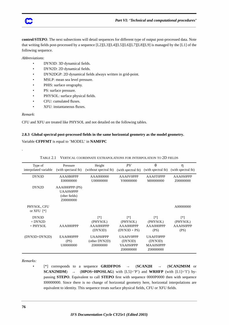
Part VI: ‘Technical and computational procedures’
. Note
he
ce
s are
control/STEPO. The next subsections will detail sequences for different type of output post-processed data
that writing fields post-processed by a sequence [L2][L3][L4][L5][L6][L7][L8][L9] is managed by the [L1] of t
following sequence.
Abbreviations:
• DYN3D: 3D dynamical fields.
• DYN2D: 2D dynamical fields.
• DYN2DGP: 2D dynamical fields always written in grid-point.
• MSLP: mean sea level pressure.
• PHIS: surface orography.
• PS: surface pressure.
• PHYSOL: surface physical fields.
• CFU: cumulated fluxes.
• XFU: instantaneous fluxes.
Remark:
CFU and XFU are treated like PHYSOL and not detailed on the following tables.
2.8.3 Global spectral post-processed fields in the same horizontal geometry as the model geometry.
VariableCFPFMT is equal to ’MODEL’ inNAMFPC
.
Remarks:
• [*] corresponds to a sequenceGRIDFPOS (SCAN2H (SCAN2MSM or
SCAN2MDM ) (HPOS+HPOSLAG) with [L5]=’P’) and WRHFP (with [L1]=’I’) by-
passingSTEPO. Equivalent to callSTEPO first with sequence 0000P0000 then with sequen
I00000000. Since there is no change of horizontal geometry here, horizontal interpolation
equivalent to identity. This sequence treats surface physical fields, CFU or XFU fields.
TABLE 2.1 VERTICAL COORDINATE EXTRAPOLATIONS FOR INTERPOLATION TO2D FIELDS
Type ofinterpolated variable
Pressure(with spectaral fit)
Height(without spectral fit)
PV(with spectral fit) (with spectral fit) (with spectral fit)
DYN3D AAA0B0PPPE00000000
AAA0H0000U00000000
AAA0V0PPPY00000000
AAA0T0PPPM00000000
AAA0S0PPPZ00000000
DYN2D AAA0H0PPP (PS)UAA0S0PPP(oher fields)Z00000000
PHYSOL, CFUor XFU [*]
A00000000
DYN3D+ DYN2D+ PHYSOL AAA0H0PPP
[*](PHYSOL)
AAA0H0PPP(DYN3D)
[*](PHYSOL)
AAA0H0PPP(DYN3D + PS)
[*](PHYSOL)
AAA0H0PPP(PS)
[*](PHYSOL)
AAA0S0PPP(PS)
(DYN3D+DYN2D) EAA0H0PPP(PS)
U00000000
UAA0S0PPP(other DYN2D)
Z00000000
UAA0V0PPP(DYN3D)
YAA0S0PPPZ00000000
UAA0T0PPP(DYN3D)
MAA0S0PPPZ00000000
θ η
→ →→
76
IFS Documentation Cycle CY25r1 (Edited 2003)
Chapter 2 ‘FULL-POS post-processing and interpolation’
ect
tine
by
f model
et to
d 3D
fields,
er 2D
post-
rface
ight
even
le if
s gener-
• All sequences called bySTEPO call VPOS, but notHPOS, HPOSLAG andENDVPOS. STEPOis generally called byDYNFPOS (underCNT4), except the last call toSTEPO (where only [L1] is
non zero) which is called directly byCNT4.
• CPREP4 is never called.
• Headline of organigramme underCNT4 is generally:
• SU4FPOS• GRIDFPOS
• SCAN2H (SCAN2MSM or SCAN2MDM ) (HPOS+HPOSLAG) for
physics or CFU or XFU if post-processing of such fields is required.
• WRHFP to write post-processed physics or CFU or XFU fields.
• DYNFPOS (always called):DYNFPOS calls one or severalSTEPO sequences according
to the 3D or 2D dynamical fields to post-process (call to vertical interpolations only). Dir
spectral transforms are called for fields to be fitted. Writing on files is made by rou
WRSFP.
• STEPO (last call for the case where only [L1] is non zero); writing on files is made
routineWRSFP.
• For as the vertical coordinate, the sequence is the same either the values are a subset o
values or not.
• All 3D variables are directly interpolated by vertical interpolations underVPOS, there is no call to
ENDVPOS.
• Spectral fit is compulsory to post-process velocity potential and stream function.
• For height coordinate, the switch controlling spectral fit is not available in namelist and is s
.FALSE. when only 3D dynamical fields are post-processed. So there is no spectral fit an
dynamical fields are provided in grid-point values.
• When spectral fit is activated, post-processed fields are spectral ones for 3D dynamical
surface pressure, mean sea level pressure and orography, grid-point ones for the oth
dynamical fields, the surface physical fields, the CFU and XFU.
• For coordinate, post-processing of surface pressure is considered as a -coordinate
processing on surface ([L5]=’S’). For other vertical coordinates, post-processing of su
pressure is considered as a height coordinate post-processing on surfaceZ=0 ([L5]=’H’).
• Unavailable variables:
• Post-processing of velocity potential and stream function is not available for he
coordinate.
• Post-processing of pressure (resp. potential vorticity, potential temperature) is not made
if required for pressure (resp. potential vorticity, potential temperature) coordinate.
• Post-processing of stretching deformation and shearing deformation is not availab
FULL-POS is made in a semi-Lagrangian job.
2.8.4 Global spectral post-processed fields in a horizontal geometry different from the model geometry.
VariableCFPFMT is equal to ’GAUSS’ and variableLFPSPEC is .TRUE. inNAMFPC (pseudo-configuration
927). This configuration requires a spectral fit in the arrival geometry.
RoutineCPREP4 is always called. Organigramme has recursivity and is of the following type:CNT0 (model ge-
ometry) set-up, control routines, includingCNT4. Headline of organigramme under this call toCNT4 does
not depend on the vertical coordinate of post-processing and on the list of post-processed variables, and i
ally:
• SU4FPOS
→→ →
η η
η ηη 1=
→
77
IFS Documentation Cycle CY25r1 (Edited 2003)
Part VI: ‘Technical and computational procedures’
l
rface
it
d
and
tal
ntal
ted.
points
0 and
ll allow
ry
ess
ctical
• CPREP4• GRIDFPOS
• SCAN2H (SCAN2MSM or SCAN2MDM ) (HPOS+HPOSLAG) for
physics or CFU or XFU if post-processing of such fields is required.
• WRHFP to write post-processed physics or CFU or XFU fields on unit 91.
• DYNFPOS (always called):
• first call to STEPO: inverse Legendre transform; then (SCAN2H(SCAN2MSM or SCAN2MDM ) ): inverse Fourier transform and horizonta
interpolations (HPOS + HPOSLAG) on model -levels for grid-point model
variables (wind components, temperature, humidity, surface pressure, su
orography).
• second call toSTEPO: writing grid-point interpolated fields on model layers on un
91 (routineWRHFP).
• CNT0 (output geometry).
CNT0 (output geometry) set-up, control routines, including:
• a call to SPECFITASM under CNT1: spectral transformation of model fields (except win
components) and surface orography in unit 91, computation of spectral stream function
velocity potential on model -levels, writing of all these fields on unit 91.
• a call toCNT4.
Headline of organigramme under this call toCNT4 is generally:
• SU4FPOS• CPREP4
• GRIDFPOS• SCAN2H (SCAN2MSM or SCAN2MDM ) (HPOS+HPOSLAG) for
physics or CFU or XFU if post-processing of such fields is required (horizon
interpolations are equivalent to identity in this case).
• WRHFP to write post-processed physics or CFU or XFU fields on unit 54.
• DYNFPOS (always called):DYNFPOS calls one or severalSTEPO sequences according
to the 3D or 2D dynamical fields to post-process (call to vertical interpolations, horizo
interpolations are neutral here). Direct spectral transforms are called for fields to be fit
• STEPO (last call for the case where only [L1] is non zero, routineWRSFP).
• CNT0 (return to model geometry to continue integration if required).
Post-processed fields are written on unit 54.
Under the first call toCNT0 one finds the following sequences ofSTEPO: AAA0M0000 (vertical interpolations
on departure geometry, simple copy on model -levels), then 0000A0000 (horizontal interpolations on grid-
of the arrival geometry), then Z00000000. It is planned in the future to merge the two sequences AAA0M000
0000A0000 into one sequence AAA0A0000 but that needs some code development: such a modification wi
to save memory.
Under the second call toCNT0 one finds the same sequences ofSTEPOas in the case without change of geomet
(variableCFPFMT equal to ’MODEL’ inNAMFPC , see above).
Remarks, restrictions of use:
APACHE is called if post-processing on height or -levels.
• ENDVPOS is theoretically called if post-processing on height or -levels to post-proc
dynamical variables which are not model variables (does not work in cycles 17 and 18). In pra
→→
→ →
→→
η
→
η
→→
→ →
η
ηη
78
IFS Documentation Cycle CY25r1 (Edited 2003)
Chapter 2 ‘FULL-POS post-processing and interpolation’
tten in
l values
et to
d 3D
fields,
er 2D
e the
e the
l fit),
nd
lative
not
e
oist
loud
erand
aring
ost-
ents,
ere is
abort),
sing
oist
loud
erand
aring
ost-
configurations callingENDVPOS are not completely coded, soENDVPOS is never called for
configurations which work.
• It is necessary to post-process at least physical surface fields, in the contrary fields are not wri
the first call toCNT0 but read in the second call toCNT0 (abort when reading inexistant fields).
• Names of articles cannot be changed in namelistNAMAFN .
• For vertical coordinate, the sequence is the same either the values are a subset of mode
or not.
• Spectral fit is compulsory to post-process velocity potential and stream function.
• For height coordinate, the switch controlling spectral fit is not available in namelist and is s
.FALSE. when only 3D dynamical fields are post-processed. So there is no spectral fit an
dynamical fields are provided in grid-point values.
• When spectral fit is activated, post-processed fields are spectral ones for 3D dynamical
surface pressure, mean sea level pressure and orography, grid-point ones for the oth
dynamical fields, the surface physical fields, the CFU and XFU.
• Restrictions of use for -coordinate:
• If no change of vertical coordinate, the number of levels to be post-processed has to b
model number of levels.
• If change of set of vertical levels, the number of levels to be post-processed has to b
number of levels specified in namelistNAMFPG .
• 3D variables which can be post-processed: temperature, stream function (if spectra
velocity potential (if spectral fit), horizontal wind components, specific humidity, wi
velocity, absolute vorticity, pressure.
• Variables which cannot be post-processed: geopotential (operand range error abort), re
humidity (operand range error abort), vertical velocity (no abort but post-processing
made), divergence and vorticity (abort inFTDIRH ), potential temperature (operand rang
error abort), liquid and solid water (no abort but post-processing not made), m
irreversible adiabatic potential temperature (abort with negative value in a logarithm), c
fraction (no abort but post-processing not made), equivalent potential temperature (op
range error abort), stretching deformation (no abort but post-processing not made), she
deformation (no abort but post-processing not made), potential vorticity (no abort but p
processing not made), wet potential vorticity (no abort but post-processing not made).
• Restrictions of use for height coordinate:
• 3D variables which can be post-processed: temperature, horizontal wind compon
specific humidity, wind velocity, absolute vorticity, pressure.
• Stream function and velocity potential cannot be post-processed due to the fact that th
no spectral fit.
• Other variables which cannot be post-processed: geopotential (operand range error
relative humidity (operand range error abort), vertical velocity (no abort but post-proces
not made), divergence and vorticity (abort inFTDIRH ), potential temperature (operand
range error abort), liquid and solid water (no abort but post-processing not made), m
irreversible adiabatic potential temperature (abort with negative value in a logarithm), c
fraction (no abort but post-processing not made), equivalent potential temperature (op
range error abort), stretching deformation (no abort but post-processing not made), she
deformation (no abort but post-processing not made), potential vorticity (no abort but p
processing not made), wet potential vorticity (no abort but post-processing not made).
• Other restrictions of use:
η η
η
79
IFS Documentation Cycle CY25r1 (Edited 2003)
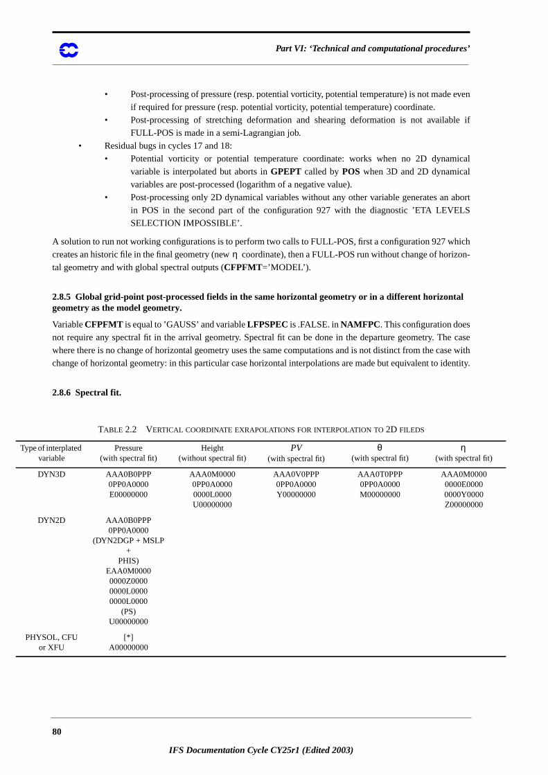
Part VI: ‘Technical and computational procedures’
even
le if
ical
abort
LS
hich
rizon-
e case
ase with
entity.
Type ofva ral fit)
DY 0000
DY
PHYSor
• Post-processing of pressure (resp. potential vorticity, potential temperature) is not made
if required for pressure (resp. potential vorticity, potential temperature) coordinate.
• Post-processing of stretching deformation and shearing deformation is not availab
FULL-POS is made in a semi-Lagrangian job.
• Residual bugs in cycles 17 and 18:
• Potential vorticity or potential temperature coordinate: works when no 2D dynam
variable is interpolated but aborts inGPEPT called byPOS when 3D and 2D dynamical
variables are post-processed (logarithm of a negative value).
• Post-processing only 2D dynamical variables without any other variable generates an
in POS in the second part of the configuration 927 with the diagnostic ’ETA LEVE
SELECTION IMPOSSIBLE’.
A solution to run not working configurations is to perform two calls to FULL-POS, first a configuration 927 w
creates an historic file in the final geometry (new coordinate), then a FULL-POS run without change of ho
tal geometry and with global spectral outputs (CFPFMT=’MODEL’).
2.8.5 Global grid-point post-processed fields in the same horizontal geometry or in a different horizontalgeometry as the model geometry.
VariableCFPFMT is equal to ’GAUSS’ and variableLFPSPEC is .FALSE. inNAMFPC . This configuration does
not require any spectral fit in the arrival geometry. Spectral fit can be done in the departure geometry. Th
where there is no change of horizontal geometry uses the same computations and is not distinct from the c
change of horizontal geometry: in this particular case horizontal interpolations are made but equivalent to id
2.8.6 Spectral fit.
TABLE 2.2 VERTICAL COORDINATE EXRAPOLATIONS FOR INTERPOLATION TO2D FILEDS
interplatedriable
Pressure(with spectral fit)
Height(without spectral fit)
PV(with spectral fit) (with spectral fit) (with spect
N3D AAA0B0PPP0PP0A0000E00000000
AAA0M00000PP0A00000000L0000U00000000
AAA0V0PPP0PP0A0000Y00000000
AAA0T0PPP0PP0A0000M00000000
AAA0M0000000E0000000Y000Z0000000
N2D AAA0B0PPP0PP0A0000
(DYN2DGP + MSLP+
PHIS)EAA0M00000000Z00000000L00000000L0000
(PS)U00000000
OL, CFU XFU
[*]A00000000
η
θ η
80
IFS Documentation Cycle CY25r1 (Edited 2003)
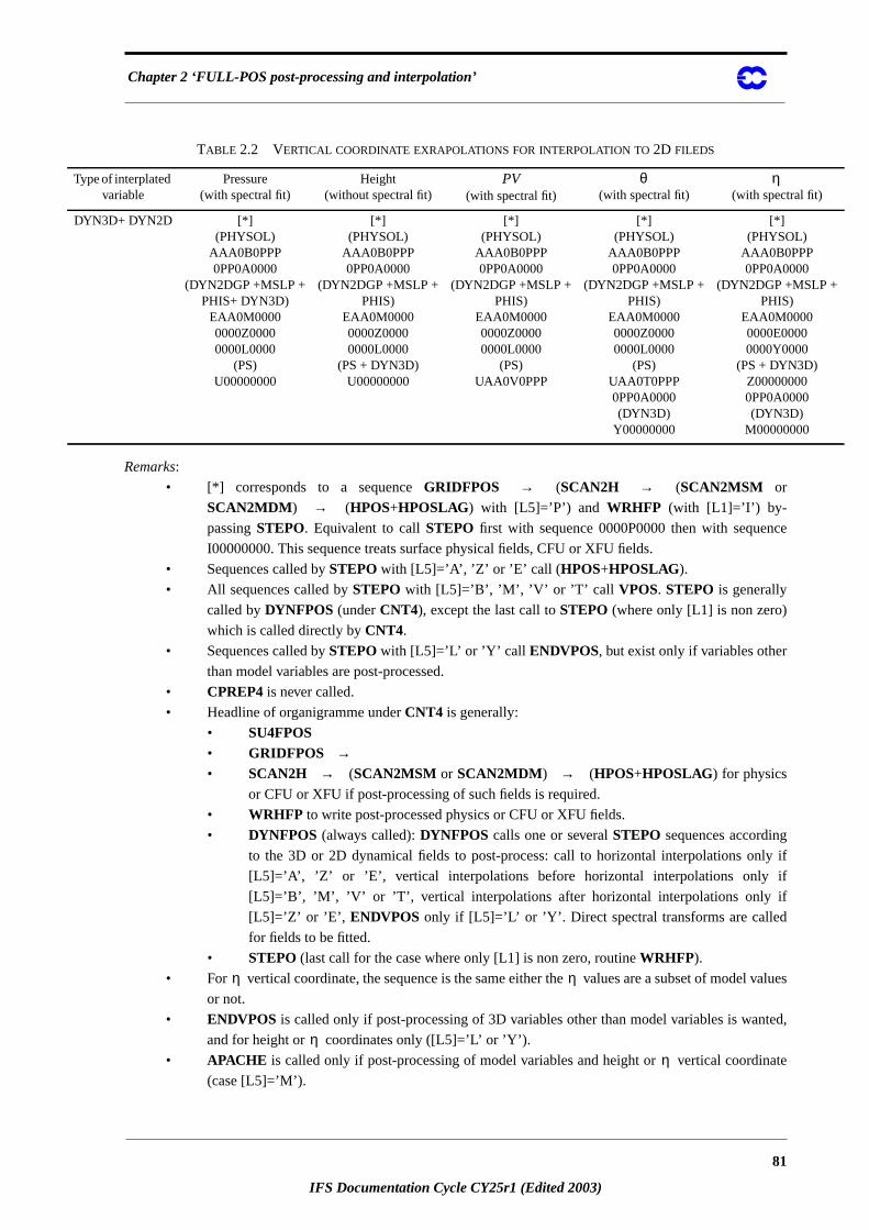
Chapter 2 ‘FULL-POS post-processing and interpolation’
ce
y if
l values
ted,
ate
DYN3D)P
00SLP +
000D)0
00
0
Type ofva al fit)
Remarks:
• [*] corresponds to a sequenceGRIDFPOS (SCAN2H (SCAN2MSM or
SCAN2MDM ) (HPOS+HPOSLAG) with [L5]=’P’) and WRHFP (with [L1]=’I’) by-
passingSTEPO. Equivalent to callSTEPO first with sequence 0000P0000 then with sequen
I00000000. This sequence treats surface physical fields, CFU or XFU fields.
• Sequences called bySTEPO with [L5]=’A’, ’Z’ or ’E’ call ( HPOS+HPOSLAG).
• All sequences called bySTEPO with [L5]=’B’, ’M’, ’V’ or ’T’ call VPOS. STEPO is generally
called byDYNFPOS (underCNT4), except the last call toSTEPO (where only [L1] is non zero)
which is called directly byCNT4.
• Sequences called bySTEPOwith [L5]=’L’ or ’Y’ call ENDVPOS, but exist only if variables other
than model variables are post-processed.
• CPREP4 is never called.
• Headline of organigramme underCNT4 is generally:
• SU4FPOS• GRIDFPOS• SCAN2H (SCAN2MSM or SCAN2MDM ) (HPOS+HPOSLAG) for physics
or CFU or XFU if post-processing of such fields is required.
• WRHFP to write post-processed physics or CFU or XFU fields.
• DYNFPOS (always called):DYNFPOS calls one or severalSTEPO sequences according
to the 3D or 2D dynamical fields to post-process: call to horizontal interpolations onl
[L5]=’A’, ’Z’ or ’E’, vertical interpolations before horizontal interpolations only if
[L5]=’B’, ’M’, ’V’ or ’T’, vertical interpolations after horizontal interpolations only if
[L5]=’Z’ or ’E’, ENDVPOS only if [L5]=’L’ or ’Y’. Direct spectral transforms are called
for fields to be fitted.
• STEPO (last call for the case where only [L1] is non zero, routineWRHFP).
• For vertical coordinate, the sequence is the same either the values are a subset of mode
or not.
• ENDVPOS is called only if post-processing of 3D variables other than model variables is wan
and for height or coordinates only ([L5]=’L’ or ’Y’).
• APACHE is called only if post-processing of model variables and height or vertical coordin
(case [L5]=’M’).
+ DYN2D [*](PHYSOL)
AAA0B0PPP0PP0A0000
(DYN2DGP +MSLP +PHIS+ DYN3D)
EAA0M00000000Z00000000L0000
(PS)U00000000
[*](PHYSOL)
AAA0B0PPP0PP0A0000
(DYN2DGP +MSLP +PHIS)
EAA0M00000000Z00000000L0000
(PS + DYN3D)U00000000
[*](PHYSOL)
AAA0B0PPP0PP0A0000
(DYN2DGP +MSLP +PHIS)
EAA0M00000000Z00000000L0000
(PS)UAA0V0PPP
[*](PHYSOL)
AAA0B0PPP0PP0A0000
(DYN2DGP +MSLP +PHIS)
EAA0M00000000Z00000000L0000
(PS)UAA0T0PPP0PP0A0000(DYN3D)
Y00000000
[*](PHYSOL
AAA0B0PP0PP0A00
(DYN2DGP +MPHIS)
EAA0M0000000E0000000Y000
(PS + DYN3Z00000000PP0A00(DYN3D)
M0000000
TABLE 2.2 VERTICAL COORDINATE EXRAPOLATIONS FOR INTERPOLATION TO2D FILEDS
interplatedriable
Pressure(with spectral fit)
Height(without spectral fit)
PV(with spectral fit) (with spectral fit) (with spectr
θ η
→ →→
→→ →
η η
ηη
81
IFS Documentation Cycle CY25r1 (Edited 2003)
Part VI: ‘Technical and computational procedures’
et to
t if
post-
00).
height
ectral
ven if
even
le if
• Spectral fit is compulsory to post-process velocity potential and stream function.
• For height coordinate, the switch controlling spectral fit is not available in namelist and is s
.FALSE. when only 3D dynamical fields are post-processed. So there is no spectral fit.
• For coordinate, there is no spectral fit for 3D dynamical variables, switchLFITS is not used.
• When spectral fit is activated, post-processed fields are fitted for 3D dynamical fields (excep
vertical coordinate), mean sea level pressure and orography.
• For coordinate, post-processing of surface pressure is considered as a -coordinate
processing on surface (sequence [L1]AA0M0000 followed by 0000E0000 + 0000Y00
For other vertical coordinates, post-processing of surface pressure is considered as a
coordinate post-processing on surfaceZ=0 (sequence [L1]AA0M0000 followed by 0000Z0000 +
0000L0000).
• Restrictions of use for -coordinate or height coordinate:
• 3D variables which can be post-processed:
• TemperatureT.
• Horizontal wind componentsU andV, wind velocity.
• Specific humidity (moisture) .
• Relative humidityHU.
• Potential temperature .
• Moist (irreversible) pseudo-adiabatic potential temperature .
• Equivalent potential temperature .
• Passive scalars (maximum of three).
• Pressure .
• Possibility to post-process three additional free upper air fields.
• 3D variables which cannot be post-processed (abort due to the fact that there is no sp
fit):
• Velocity potential .
• Stream function .
• Other 3D variables which cannot be post-processed (post-processing not made e
required):
• Geopotential .
• Ice content .
• (pressure coordinate vertical velocity).
• Relative vorticity .
• DivergenceD.
• Liquid water content .
• Cloudiness .
• Absolute vorticity .
• Stretching deformationSTD.
• Shearing deformationSHD.
• Potential vorticityPV.
• Wet potential vorticity .
• Other restrictions of use:
• Post-processing of pressure (resp. potential vorticity, potential temperature) is not made
if required for pressure (resp. potential vorticity, potential temperature) coordinate.
• Post-processing of stretching deformation and shearing deformation is not availab
FULL-POS is made in a semi-Lagrangian job.
ηη
η ηη 1=
η
q
θθw
θe
phyd
ψχ
µqi
ωζ
ql
qa
ζ f+
PVw
82
IFS Documentation Cycle CY25r1 (Edited 2003)
Chapter 2 ‘FULL-POS post-processing and interpolation’
e
E/
li-
IN
case
h
ON
case
an
d
ces
d
2.8.7 No spectral fit.
Sequence [L1][L2][L3][L4][L5]0PPP followed by 0PP0[L5][L6][L7][L8][L9] is replaced by sequenc
[L1][L2][L3][L4][L5]0000 followed by 0000[L5][L6][L7][L8][L9]. Routine SPOS is no longer called.
2.8.8 Grid-point post-processed fields in a ALADIN limited area domain.
VariableCFPFMT is equal to ’LELAM’ and variableLFPSPEC is .FALSE. inNAMFPC .
Same sequences and same organigramme as in the caseCFPFMT=’GAUSS’ andLFPSPEC=.FALSE. .
2.8.9 Grid-point post-processed fields in a latitude-longitude limited area domain.
VariableCFPFMT is equal to ’LALON’ and variableLFPSPEC is .FALSE. inNAMFPC .
Same sequences and same organigramme as in the caseCFPFMT=’GAUSS’ andLFPSPEC=.FALSE. .
2.8.10 Mixed ARPEGE/IFS-ALADIN FULL-POS configurations: spectral post-processed fields in a limitedarea domain.
VariableCFPFMT is equal to ’LELAM’ and variableLFPSPEC is .TRUE. inNAMFPC (pseudo-configuration
E927). ALADIN libraries are necessary in this case (take AL07 ALADIN library and CY16T1_AL07 ARPEG
IFS library). The first call toCNT0 makes an ARPEGE/IFS run, the second one makes an ALADIN run.
Same sequences and same organigramme as in the caseCFPFMT=’GAUSS’ andLFPSPEC=.TRUE. with change
of horizontal geometry (pseudo-configuration 927).
2.8.11 Pure ALADIN FULL-POS configurations.
ALADIN libraries are necessary in this case (take AL07 ALADIN library and CY16T1_AL07 ARPEGE/IFS
brary).
• CFPFMT=’MODEL’, LFPSPEC=.FALSE.: spectral outputs on an ALADIN domain which is
identical to the model ALADIN domain. Same sequences as in the case (CFPFMT=’MODEL’,
LFPSPEC=.FALSE.) of ARPEGE/IFS. One call toCNT0, no call toCPREP4.• CFPFMT=’LELAM’, LFPSPEC=.FALSE.: grid-point outputs on an ALADIN domain which is
included in the model ALADIN domain. Cannot work if the required post-processing ALAD
domain is not included in the model ALADIN domain. Same sequences as in the
(CFPFMT=’LELAM’, LFPSPEC=.FALSE.) of ARPEGE/IFS. One call toCNT0, no call to
CPREP4.• CFPFMT=’LALON’, LFPSPEC=.FALSE.: grid-point outputs on some LALON domains whic
are included in the model ALADIN domain. Cannot work if the required post-processing LAL
domains are not included in the model ALADIN domain. Same sequences as in the
(CFPFMT=’LALON’, LFPSPEC=.FALSE.) of ARPEGE/IFS. One call toCNT0, no call to
CPREP4.• CFPFMT=’GAUSS’, LFPSPEC=.FALSE. has no sense for ALADIN.
• CFPFMT=’LELAM’, LFPSPEC=.TRUE.: pseudo-configuration EE927, spectral outputs on
ALADIN domain which is included in the model ALADIN domain. Cannot work if the require
post-processing ALADIN domain is not included in the model ALADIN domain. Same sequen
as in the cases (CFPFMT=’LELAM’, LFPSPEC=.TRUE.) of the pseudo-configurations 927 en
E927. Two calls toCNT0 with LELAM =.T., CPREP4 is called.
83
IFS Documentation Cycle CY25r1 (Edited 2003)
Part VI: ‘Technical and computational procedures’
-
ex-
titudes
d and
he
ture nec-
model
int.
hus in-
" model
h
-
d south
2.9 SOME SHARED MEMORY FEATURES :
2.9.1 Calculations packets:
Grid-point computations:
In the grid-point space there is a subdivision of the grid-points intoNSLBR+NDGSURpackets of lengthNPRO-MA (the useful number of values in each packet is lower or equal thanNPROMA ). These packets contain the ex
tra-longitudes. Some packets can contain polar and extra-polar latitudes data. ANPROMA -packet always contains
a set of complete latitudes, soNPROMA is always greater or equal thanNDLON+3. For the FULL-POS there is
a second subdivision into sub-packets of lengthNFPROMAL containingNFPROFuseful points for computations
at the points of the arrival horizontal geometry (routinesSURFPBUF, SUWFPBUF, HPOSLAG andENDV-POS). More details will be given later for the data transmission for horizontal interpolations.
One 2D field hasNGPTOT points.NGPTOT does not take account of the extra-longitudes, the poles and the
tra-polar latitudes. When counting the additional points due to extra-longitudes, poles and the extra-polar la
one obtains a total amount ofNBDYSZ points. For shared memory the variablesNGPTOTG andNGPTOTMXare equal toNGPTOT. All these variables take account of the reduced Gaussian/Lobatto grid. It is assume
hardcoded that there are one western extra-longitude and two eastern extra-longitudes. Longitudejlon=1 is always
the “Greenwich" meridian of the computational sphere.
Fourier transforms:
Fourier transforms are done latitude by latitude for eachNPROMA -packet. Data reorganisation is necessary in t
Fourier space between the zonal wave structure necessary for Legendre transforms and the latitudinal struc
essary for Fourier transforms.
Legendre transforms:
Legendre transforms are done zonal wave number by zonal wave number.
Filtering in spectral space:
Filtering in spectral space is done zonal wave number by zonal wave number. A call toSPOScurrently treats only
one zonal wave number.
2.9.2 Transmission of data necessary for FULL-POS horizontal interpolations from HPOS to HPOSLAG:interpolation buffers.
First one associates to each interpolation point, which is generally not a model grid-point, an “associated"
grid-point which currently satisfies to the following rule:
• the “associated" model grid-point is on the longitude immediately west to the interpolation po
• the “associated" model grid-point is on the latitude immediately south to the interpolation.
Interpolations use data of points which are not necessary on the same latitude as the interpolation point. T
terpolation routines need to have access to a limited number of latitudes north and south of the “associated
grid-point latitude. Interpolation points are collected so that a call toHPOSLAG for horizontal interpolations treats
a set of points (defined by the two arraysNFPBSRandNFPROF), the “associated" model grid-points set of whic
is a model package of latitudes (of dimension lower or equal thanNPROMA ), so one can name this set of grid
points the “associated" model grid-point package of latitudes. The number of packages of latitudes north an
of the “associated" model grid-point package of latitudes is precomputed in the subroutineSUSC2so as the grid-
points necessary for interpolations are always in this set of packages of latitudes. For example, if one needsN pack-
ages of latitudes north andN packages of latitudes south (N is stored in variableNFPWIDE ) of the “associated"
84
IFS Documentation Cycle CY25r1 (Edited 2003)
Chapter 2 ‘FULL-POS post-processing and interpolation’
e
r
s are
art and
s
t of
ray
vari-
m-
in the
he
des
model grid-point package of latitudes (which is denoted bynlat), computations of interpolation quantities (mad
in subroutineHPOS) must be performed for the packages of latitudesnlat-N to nlat+N before making interpola-
tions of points, the “associated" model grid-point of which is localised on the package of latitudes numbenlat.
This is the reason of splitting the grid-point computations into two parts, one non-lagged part (HPOS) and one
lagged part (HPOSLAG). Quantities to be interpolated are computed in the non-lagged part and interpolation
performed in the lagged part. Of course all grid-point data are not kept in memory between the non-lagged p
the lagged part, in order to save memory (and use the input-output scheme). Data for packages of latitudenlat-N
to nlat+N is stored in interpolation buffer arrays calledPFPBUF1 andPFPBUF2 in HPOS, HPOSLAG and
SCAN2MSM and local arraysZFPBUF1 andZFPBUF2 in the routineSCAN2H. The following considerations
made forPFPBUF1 are valid forPFPBUF2.
PFPBUF1contains the buffers for some variables to be interpolated. The first dimension ofPFPBUF1 is NPRO-MA . (NPROMA is above the maximum number of longitudes per latitude + 3 and is defined in the namelistNAM-DYN and is used to dimension arrays containing only data of the package of latitudesnlat). The second dimension
of PFPBUF1 is the number of 2D horizontal fields to be horizontally interpolated. The second elemen
PFPBUF1 is used to identify the the FULL-POS quantity to be interpolated (local variableIFLD computed in
HPOS). The third dimension ofPFPBUF1is NFPB1(dummy variableKFPB1 in HPOS), to make available a set
of latitudes (nlat-N to nlat+N) in the lagged part of the grid-point computations. The third element of ar
PFPBUF1for storage of the current latitudenlat is denoted by the local integer variableIB1 in HPOSandHPO-SLAG. NFPB1 is computed in the set-up routineSUSIZBUF called bySUSC2in a rather complicated way. Its
value is close (but not always equal) to 2N+NTASKS+NDGSUR (NTASKS is the number of tasks,NDGSUR is
the number of extra-latitudes). Attribution of buffers is made underHPOS by calling the functionMGETBUF :
this function searches for a free buffer to store the data currently treated byHPOS; if there is no free buffer routine
MGETBUF generates anABOR1 and that means thatNFPB1 has an unsufficient value.
Fig. 2.3 shows how data is arranged in interpolation buffers in the case of asking for post-processing of two
ablesX andY on four layers numbered 1, 2, 3, 4,N=2, in the non-lagged and lagged parts of the grid-point co
putations.IFLDX and IFLDY are the corresponding second dimension in arrayPB1 corresponding to layer
number 1.F is a mapping: packages of latitudes are not necessary in order in the interpolation buffer arrays
lagged part of grid-point computations. In the example shown in figure 11.1:
• F(nlat-2) = nlat+2
• F(nlat-1) = nlat-2
• F(nlat ) = nlat-1
• F(nlat+1) =nlat• F(nlat+2) =nlat+1
i.e. buffer 1 containsnlat+2 data, ..., buffer 5 containsnlat+1 data. In interpolation routines one needs to know t
number of the buffer where data corresponding to a latitude denoted byJGL can be found. This information is
computed inHPOSLAG by calling functionMFINDBUF , before interpolations, and stored in the arrayIBUFP1.
In the example shown in figure 11.1, that gives:
• if latitudeJGL is in the package of latitudesnlat-2, IBUFP1(JGL )=2.
• if latitudeJGL is in the package of latitudesnlat-1, IBUFP1(JGL )=3.
• if latitudeJGL is in the package of latitudesnlat , IBUFP1(JGL )=4.
• if latitudeJGL is in the package of latitudesnlat+1, IBUFP1(JGL )=5.
• if latitudeJGL is in the package of latitudesnlat+2, IBUFP1(JGL )=1.
In this example the local variableIB1 is equal to 4 inHPOSandHPOSLAG. When interpolations are doneHPO-SLAG calls a functionMDONEBUF which searches for the useless buffers: if data for the package of latitu
nlat-2 becomes useless for the following interpolationsMDONEBUF sends a sort of message thatIBUFP1=2 (the
85
IFS Documentation Cycle CY25r1 (Edited 2003)
Part VI: ‘Technical and computational procedures’
are
s.
-
o-
etween
(cor-
es
ints.
.
t
r MIO
buffer number 2) will be free to store data of another package of latitudes when calling againHPOS.
Set-up routinesCPCLIMI andCPCLIMO use the same logics but in a simpler way: all interpolation buffers
completely filled for all latitudes before the interpolations, so functionsMGETBUF , MFINDBUF and
MDONEBUF are not used. Similar features are used inFPMODPREC to modify the precipitations before inter-
polations: an interpolation buffer and some routines coded like interpolation routines (FPSCAW2, FPOLIS) are
used.
One uses arrays with horizontal dimensionNPROMA . OneNPROMA -length array can contain several latitude
In interpolation routines one needs to know the positionJROF in a NPROMA -dimensionned array of data con
cerning the point of coordinates (longitude number=JLON , latitude number=JGL ). The arrayNSTABUF com-
puted in subroutineSUSC2 gives this information:JROF=JLON+NSTABUF(JGL ).
Contrary to what occurs in the semi-Lagrangian scheme, the number of interpolation points (variableNFPRGPL)
is not equal to the number of model grid-points (variableNGPTOT). So there is no mapping between the interp
lations points and the model grid-points contrary to the semi-Lagrangian scheme where there is a mapping b
the interpolation point (origin or medium point of the semi-Lagrangian trajectory) and the model grid-point
responding arrival point of the semi-Lagrangian trajectory). So there is need to associate to theNPROMA packets
a certain amount of FULL-POS interpolation points which are subdivised intoNFPBSRsubpackets of length low-
er or equal thanNFPROMAL (the actual length is inNFPROF). Computations are made in the set-up routin
SUFPSC2 andSUFPSC2B. In SUFPSC2 one computes:
• for each NPROMA -packet numberjslbr: NFPLENR(jslbr) is the number of post-processing
points associated to theNPROMA -packet numberjslbr. Some statistics aboutNFPLENR are
printed (mean, minimum, maximum, standard deviation, number of zero values ofNFPLENR).
• then one definesNFPROMAL which will control the additional subdivision.
• then one computes the numberNFPBSRof subpackets necessary to store all theNFPLENR values
in aNFPROMAL -dimensioned array.
• NFPSTAP is used to count the total number of sub-packets for all the post-processing po
NFPSTAP(jslbr) is the total number of subpackets for all theNPROMA -packets numbered from
NDGSAG to jslbr-1.
In SUFPSC2B:• for each sub-packetjbsr from 1 to NFPBSR(jslbr) one computes the number of FULL-POS
interpolated data to be stored (arrayNFPROF); the current rule is:NFPROF(NFPSTAP(jslbr)+1)
to NFPROF(NFPSTAP(jslbr)+NFPBSR(jslbr)-1) are equal to NFPROMAL ,
NFPROF(NFPSTAP(jslbr)+NFPBSR(jslbr)) is equal to the remaining number of points to store
• for each post-processing point numberjfp: if jfp2 is the position in a dataset of lengthNFPROF,
jslbr the number of the associatedNPROMA -packet andjbsr the number of the sub-packe
between 1 toNFPBSR(jslbr), the arrayNFPSORT provides the informationNFPSORT(jfp2,
NFPSTAP(jslbr)+jbsr) = jfp
• some other quantities are computed to store or read interpolated FULL-POS data in buffers o
files using the routinesSC2RDG andSC2WRG.
86
IFS Documentation Cycle CY25r1 (Edited 2003)
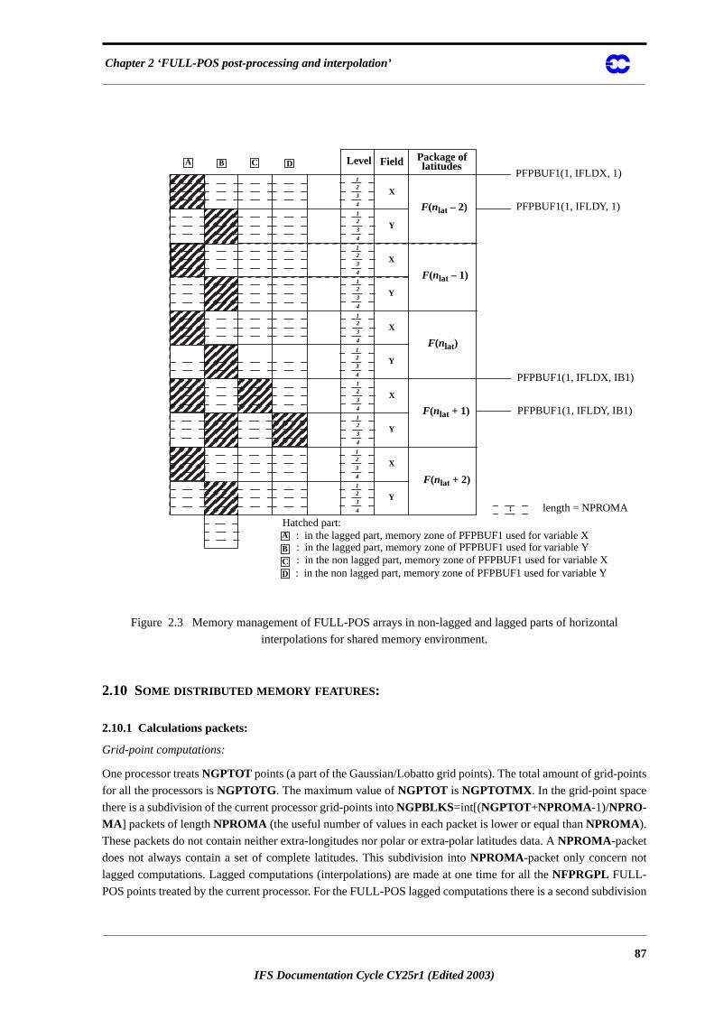
Chapter 2 ‘FULL-POS post-processing and interpolation’
l
ints
division
Figure 2.3 Memory management of FULL-POS arrays in non-lagged and lagged parts of horizonta
interpolations for shared memory environment.
2.10 SOME DISTRIBUTED MEMORY FEATURES :
2.10.1 Calculations packets:
Grid-point computations:
One processor treatsNGPTOT points (a part of the Gaussian/Lobatto grid points). The total amount of grid-po
for all the processors isNGPTOTG. The maximum value ofNGPTOT is NGPTOTMX . In the grid-point space
there is a subdivision of the current processor grid-points intoNGPBLKS=int[(NGPTOT+NPROMA -1)/NPRO-MA ] packets of lengthNPROMA (the useful number of values in each packet is lower or equal thanNPROMA ).
These packets do not contain neither extra-longitudes nor polar or extra-polar latitudes data. ANPROMA -packet
does not always contain a set of complete latitudes. This subdivision intoNPROMA -packet only concern not
lagged computations. Lagged computations (interpolations) are made at one time for all theNFPRGPL FULL-
POS points treated by the current processor. For the FULL-POS lagged computations there is a second sub
123
4
123
4
123
4
123
4
123
4
123
4
123
4
123
4
123
4
123
4
X
Y
X
Y
X
Y
X
Y
X
Y
Level Field Package oflatitudes
F(nlat – 2)
F(nlat – 1)
F(nlat)
F(nlat + 1)
F(nlat + 2)
A
B
CD
A B D
Hatched part:: in the lagged part, memory zone of PFPBUF1 used for variable X: in the lagged part, memory zone of PFPBUF1 used for variable Y: in the non lagged part, memory zone of PFPBUF1 used for variable X: in the non lagged part, memory zone of PFPBUF1 used for variable Y
CPFPBUF1(1, IFLDX, 1)
PFPBUF1(1, IFLDY, 1)
PFPBUF1(1, IFLDX, IB1)
PFPBUF1(1, IFLDY, IB1)
length = NPROMA
87
IFS Documentation Cycle CY25r1 (Edited 2003)
Part VI: ‘Technical and computational procedures’
e
western
int are
oint com-
s,
or Legen-
nal wave
the time.
model
int.
nt if
sian/
his as-
polation
gitudes
o
of
t proc-
e per-
nor
into sub-packets of lengthNFPROMAL containingNFPROF useful points for computations at the points of th
arrival horizontal geometry (routinesSURFPBUF, SUWFPBUF, HPOSLAG andENDVPOS). More details will
be given later for the data transmission for horizontal interpolations. One 2D field hasNGPTOTG points divided
into NPROCA*NPROCB sets ofNGPTOT points treated by each processor.NGPTOT does not take account of
the extra-longitudes, the poles and the extra-polar latitudes. VariableNBDYSZ is equal toNGPTOT. All these var-
iables take account of the reduced Gaussian/Lobatto grid. It is assumed and hardcoded that there are one
extra-longitude and two eastern extra-longitudes. The DM-global longitudejlon=1 is always the “Greenwich" me-
ridian of the computational sphere. All the vertical levels and the variables corresponding to a same grid-po
treated by the same processor. There are necessary transpositions (reorganisation of data) between grid p
putations and Fourier transforms because Fourier transforms need complete latitudes.
Fourier transforms:
Fourier transforms are done latitude by latitude for eachNPROMA -packet. A processor treats a subset of latitude
one latitude at the time. A processor can treat only a subset of the vertical levels (ifNPROCB>1). Data reorgani-
sation and transpositions are necessary in the Fourier space between the zonal wave structure necessary f
dre transforms and the latitudinal structure necessary for Fourier transforms.
Legendre transforms:
Legendre transforms are done zonal wave number by zonal wave number. A processor treats a subset of zo
numbers, one zonal wave number at the time.
Filtering in spectral space:
Filtering in spectral space is done zonal wave number by zonal wave number. A call toSPOScurrently treats only
one zonal wave number. A processor treats a subset of zonal wave numbers, one zonal wave number at
2.10.2 Transmission of data necessary for FULL-POS horizontal interpolations from HPOS to HPOSLAG:interpolation buffers.
First one associates to each interpolation point, which is generally not a model grid-point, an “associated"
grid-point which currently satisfies to the following rule:
• the “associated" model grid-point is on the longitude immediately west to the interpolation po
• the “associated" model grid-point is on the latitude immediately north to the interpolation poi
the interpolation point is not between the Gaussian/Lobatto North pole and the first Gaus
Lobatto latitude; in the contrary one takes the first Gaussian/Lobatto latitude.
This associated model grid-point is always between the latitudes 1 andNDGLG (it is never a pole or an extra-polar
latitude point). The processor which treats the FULL-POS interpolation point is the processor which treats t
sociated model grid-point.
Interpolations use data of points which are not necessary on the same latitude and longitude as the inter
point. Thus interpolation routines need to have access to a limited number of surrounding latitudes and lon
which are not necessary treated by the current processor. Interpolation points are collected so that a call tHPO-SLAG for horizontal interpolations treats a set of points (defined by the two arraysNFPBSRandNFPROF), the
“associated" model grid-points set of which is aNGPTOT set which is treated by one processor. The number
surrounding latitudes and longitudes rows necessary for interpolations but which do not belong to the curren
essor is precomputed in the subroutineSUSC2(variableNFPWIDE ). This is a sort of “halo" belonging to some
other processors. Due to the “halo" there is still need to split calculations into not lagged ones (HPOS) and lagged
ones (HPOSLAG). Quantities to be interpolated are computed in the non-lagged part and interpolations ar
formed in the lagged part. InHPOS, only data of the current processor (without any extra-longitudinal data
88
IFS Documentation Cycle CY25r1 (Edited 2003)
Chapter 2 ‘FULL-POS post-processing and interpolation’
se
ption is
buffers
e
ll
l
he
u-
o
lation
ry
ket
varia-
e as
polar and extra-polar data) are computed. For all theNPROMA -packages treated by the current processor the
data are stored in the arraysPFPBUF1 and PFPBUF2 in HPOS (also calledPFPBUF1 and PFPBUF2 in
SCAN2MDM ). Then some communication routines are called inSCAN2MDM to constitute the halo.FPADD3Pdoes a memory transfer in a bigger interpolation buffer where some place is let for extra-longitudes (assum
made that interpolations use only the data of 2 longitudes west and 2 longitudes east) and the halo (
ZFPBUF1 andZFPBUF2 in SCAN2MDM ). FPREAD andFPWRIT do processor communication to constitut
the halo (receives and sends data from some other processors).FPEXTPOL add data of extra-polar latitudes in the
halo when necessary. The first dimension ofZFPBUF1 andZFPBUF2 is NAFPB1 which is the total number of
points one needs for the interpolations (NAFPB1 is greater thanNGPTOT). The second dimension ofZFPBUF1andZFPBUF2 is the same as forPFPBUF1andPFPBUF2: the number of 2D fields to be interpolated. When a
theNAFPB1 dataset is constituted, the lagged partHPOSLAG is called which do horizontal interpolations for al
theNFPRGPL to be interpolated.
Contrary to the shared memory case, theNPROMA -packets subdivision no longer exist in the lagged part of t
computations (HPOSLAG, ENDVPOS) for distributed memory, the only subdivision existing for lagged comp
tations is theNFPROMAL -packets one. FunctionsMGETBUF , MFINDBUF andMDONEBUF are useless. It
is planned in the future to reintroduce an intermediateNPROMA subdivision for lagged computations, in order t
save memory, especially if there are a few numbers of processors.
Set-up routinesCPCLIMI andCPCLIMO use the same logics. Similar features are used inFPMODPREC to
modify the precipitations before interpolations: an interpolation buffer and some routines coded like interpo
routines (FPSCAW2, FPOLIS) are used.
Concerning the computations ofSUFPSC2andSUFPSC2B, the principal change compared to shared memo
case is that there is no intermediateNPROMA -packets subdivision for interpolations, so there is only one pac
jslbr=1 ofNFPRGPL FULL-POS interpolations points which is divided intoNFPBSRsubpackets of length lower
or equal thanNFPROMAL . That make simpler the computations inSUFPSC2andSUFPSC2B. Remaining con-
siderations are the same. For details about the calculations done inSUFPSC2andSUFPSC2B, see the correspond-
ing description of the shared memory case, replace ’jslbr varies fromNDGSAG to NSLBR’ by ’ jslbr=1’.
2.11 PARAMETER VARIABLES TO BE KNOWN :
2.11.1 Parameter PARFPOS.
Contains basic dimensions for FULL-POS post-processing (in parenthesis, value currently attributed). All
bles are DM-global.
• JPOSDOM : maximum number of horizontal (sub)domains (15).
• JPOSFRQ: maximum number of output frequencies (10).
• JPOSLEN : maximum length of a (sub)domain name (7).
• JPOSLIS : maximum number of groups of subdomains (10).
• JPOSDIR : maximum length of the path (or prefix) for the output files (180).
• JPOSLE : maximum number of -levels on the output subdomain (200, same asJPMXLE ).
• JPOSGL : maximum number of latitude rows of the output Gaussian/Lobatto grid (1001, sam
JPMXGL ).
• JPOS3DF: maximum number of specific 3D dynamical fields (45).
• JPOSSCVA: maximum number of post-processable passive scalars (3).
• JPOS2DF: maximum number of specific 2D dynamical fields (15).
• JPOSPHY : maximum number of surface fields (110).
η
89
IFS Documentation Cycle CY25r1 (Edited 2003)
Part VI: ‘Technical and computational procedures’
ised in
sion
• JPOSCFU: maximum number of cumulated fluxes (60).
• JPOSXFU : maximum number of instantaneous fluxes (50).
• JPOS3P: maximum number of post-processing pressure levels (30).
• JPOS3H: maximum number of post-processing height (above orography) levels (65).
• JPOS3TH : maximum number of post-processing potential temperature levels (10).
• JPOS3PV: maximum number of post-processing potential vorticity levels (10).
• JPOS3S: maximum number of post-processing -levels (200, same asJPOSLE).
• JPOSVSO: maximum number of climatologic fields of output format (20).
2.12 COMMON /MODULE AND NAMELIST VARIABLES TO BE KNOWN :
2.12.1 PTRFPB2.
Contains variables and pointers for grid point fields used for horizontal post-processing. Variables are initial
setup routinesetup/SUFPSC2B. No variable in namelist. All variables are DM-global.
List of variables:
• NFPVT0: number of auxiliary surface grid point fields.
• MATS0 : pointer for output surface temperature.
• MATSI : pointer for interpolated surface temperature.
• MAHS0 : pointer for output surface relative moisture.
• MASDO : pointer for (standard deviation of orography)*g.
• MADOU : pointer for zonal component of topography principal axis.
• MADOV : pointer for meridian component of topography principal axis.
• MAACT : pointer for anisotropy coefficient of topography.
PTRFPB2has to be split later intoYOMFPB2 containingNFPVT0 and a pointer (directorypointer) PTRFPB2containing pointers.
2.12.2 YOM4FPOS.
Contains variables relative to FULL-POS working arrays (level 4). Variables are initialised in setup routinesetup/SU4FPOS. No variable in namelist. All variables are DM-global.
Post-processing on 3D dynamical variables:
• NTFPP : total number of fields in pressure levels.
• NTFPH : total number of fields in height levels.
• NTFPTH : total number of fields in -levels.
• NTFPPV: total number of fields in potential vorticity levels.
• NTFPS : total number of fields in -levels.
• NOFPP : total number of pressure levels for each field. Array of dimensionNFP3DF.
• NOFPH : total number of height levels for each field. Array of dimensionNFP3DF.
• NOFPTH: total number of -levels for each field. Array of dimensionNFP3DF.
• NOFPPV: total number of potential vorticity levels for each field. Array of dimensionNFP3DF.
• NOFPS: total number of -levels for each field. Array of dimensionNFP3DF.
• NAFPP : total number of subdomains for each pressure level of each field. Array of dimen
(NFP3P,NFP3DF).
η
θ
η
θ
η
90
IFS Documentation Cycle CY25r1 (Edited 2003)
Chapter 2 ‘FULL-POS post-processing and interpolation’
ion
ion
of
ion
ion
on
n
on
n
on
• NAFPH : total number of subdomains for each height level of each field. Array of dimens
(NFP3H,NFP3DF).
• NAFPT : total number of subdomains for each -level of each field. Array of dimens
(NFP3TH,NFP3DF).
• NAFPV : total number of subdomains for each potential vorticity level of each field. Array
dimension (NFP3PV,NFP3DF).
• NAFPS : total number of subdomains for each -level of each field. Array of dimens
(NFP3S,NFP3DF).
• NCPFP : field pointers in pressure levels. Array of dimensionNFP3DF.
• NCHFP : field pointers in height levels. Array of dimensionNFP3DF.
• NCTFP : field pointers in -levels. Array of dimensionNFP3DF.
• NCVFP : field pointers in potential vorticity levels. Array of dimensionNFP3DF.
• NCSFP: field pointers in -levels. Array of dimensionNFP3DF.
• NPFP : pressure level pointers for each field. Array of dimension (NFP3P,NFP3DF).
• NHFP : height level pointers for each field. Array of dimension (NFP3H,NFP3DF).
• NTFP : -level pointers for each field. Array of dimension (NFP3TH,NFP3DF).
• NVFP : potential vorticity level pointers for each field. Array of dimension (NFP3PV,NFP3DF).
• NSFP: -level pointers for each field. Array of dimension (NFP3S,NFP3DF).
• NIPFP : subdomain index for each pressure level of each field. Array of dimens
(NFPDOM,NFP3P,NFP3DF).
• NIHFP : subdomain index for each height level of each field. Array of dimensi
(NFPDOM,NFP3H,NFP3DF).
• NITFP : subdomain index for each -level of each field. Array of dimensio
(NFPDOM,NFP3TH,NFP3DF).
• NIVFP : subdomain index for each potential vorticity level of each field. Array of dimensi
(NFPDOM,NFP3PV,NFP3DF).
• NISFP : subdomain index for each -level of each field. Array of dimensio
(NFPDOM,NFP3S,NFP3DF).
Post-processing on 2D dynamical variables:
• NOFP2F: total number of 2D fields.
• NOFP2A: total number of subdomains for each 2D field. Array of dimensionNFP2DF.
• NC2FP : 2D field pointers. Array of dimensionNFP2DF.
• NI2FP : subdomain index for each 2D field. Array of dimension (NFPDOM,NFP2DF).
Post-processing on lagged physical and instantaneous fluxes variables:
• NPHYFPB9: number of physical fields.
• NXFUFPB9: number of instantaneous fluxes.
• NAPHYFP9: number of subdomains for each physical field. Array of dimensionNFPPHY.
• NAXFUFP9: number of subdomains for each instantaneous flux. Array of dimensionNFPXFU.
• NCPHYFP9: field pointers of physics. Array of dimensionNFPPHY.
• NCXFUFP9: field pointers of instantaneous fluxes. Array of dimensionNFPXFU.
• NIPHYFP9: subdomain index for each physical field. Array of dimension (NFPDOM,NFPPHY).
• NIXFUFP9: subdomain index for each instantaneous flux. Array of dimensi
(NFPDOM,NFPXFU).
θ
η
θ
η
θ
η
θ
η
91
IFS Documentation Cycle CY25r1 (Edited 2003)
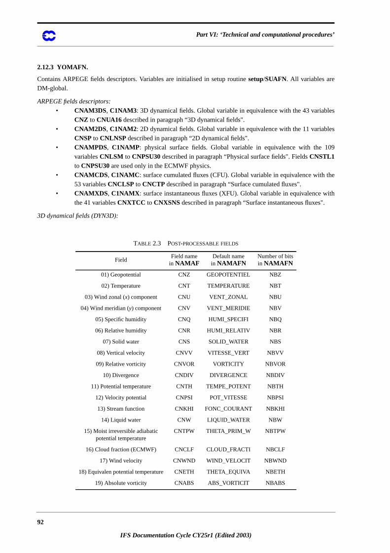
Part VI: ‘Technical and computational procedures’
les
les
09
the
ith
2.12.3 YOMAFN.
Contains ARPEGE fields descriptors. Variables are initialised in setup routinesetup/SUAFN. All variables are
DM-global.
ARPEGE fields descriptors:
• CNAM3DS, C1NAM3: 3D dynamical fields. Global variable in equivalence with the 43 variab
CNZ to CNUA16 described in paragraph “3D dynamical fields".
• CNAM2DS, C1NAM2: 2D dynamical fields. Global variable in equivalence with the 11 variab
CNSP to CNLNSP described in paragraph “2D dynamical fields".
• CNAMPDS, C1NAMP: physical surface fields. Global variable in equivalence with the 1
variablesCNLSM to CNPSU30described in paragraph “Physical surface fields". FieldsCNSTL1to CNPSU30are used only in the ECMWF physics.
• CNAMCDS, C1NAMC : surface cumulated fluxes (CFU). Global variable in equivalence with
53 variablesCNCLSP to CNCTP described in paragraph “Surface cumulated fluxes".
• CNAMXDS , C1NAMX : surface instantaneous fluxes (XFU). Global variable in equivalence w
the 41 variablesCNXTCC to CNXSNS described in paragraph “Surface instantaneous fluxes".
3D dynamical fields (DYN3D):
TABLE 2.3 POST-PROCESSABLE FIELDS
FieldField name
in NAMAFDefault name
in NAMAFNNumber of bitsin NAMAFN
01) Geopotential CNZ GEOPOTENTIEL NBZ
02) Temperature CNT TEMPERATURE NBT
03) Wind zonal (x) component CNU VENT_ZONAL NBU
04) Wind meridian (y) component CNV VENT_MERIDIE NBV
05) Specific humidity CNQ HUMI_SPECIFI NBQ
06) Relative humidity CNR HUMI_RELATIV NBR
07) Solid water CNS SOLID_WATER NBS
08) Vertical velocity CNVV VITESSE_VERT NBVV
09) Relative vorticity CNVOR VORTICITY NBVOR
10) Divergence CNDIV DIVERGENCE NBDIV
11) Potential temperature CNTH TEMPE_POTENT NBTH
12) Velocity potential CNPSI POT_VITESSE NBPSI
13) Stream function CNKHI FONC_COURANT NBKHI
14) Liquid water CNW LIQUID_WATER NBW
15) Moist irreversible adiabaticpotential temperature
CNTPW THETA_PRIM_W NBTPW
16) Cloud fraction (ECMWF) CNCLF CLOUD_FRACTI NBCLF
17) Wind velocity CNWND WIND_VELOCIT NBWND
18) Equivalen potential temperature CNETH THETA_EQUIVA NBETH
19) Absolute vorticity CNABS ABS_VORTICIT NBABS
92
IFS Documentation Cycle CY25r1 (Edited 2003)
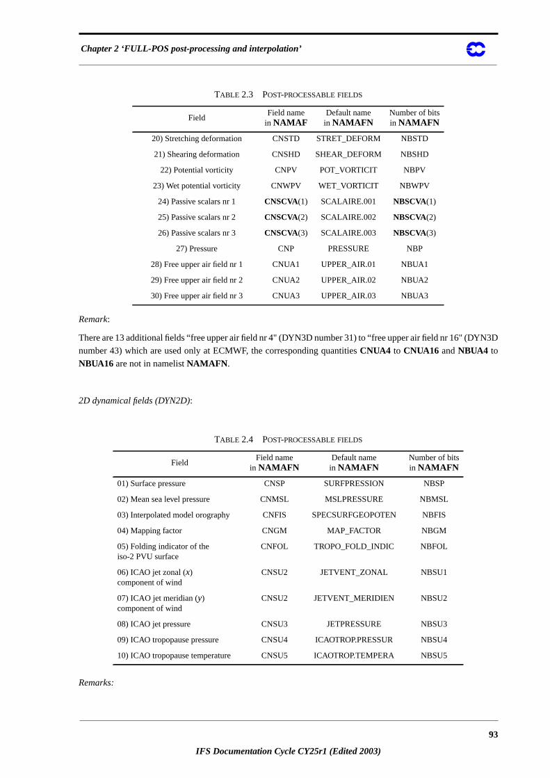
Chapter 2 ‘FULL-POS post-processing and interpolation’
3D
Remark:
There are 13 additional fields “free upper air field nr 4" (DYN3D number 31) to “free upper air field nr 16" (DYN
number 43) which are used only at ECMWF, the corresponding quantitiesCNUA4 to CNUA16 andNBUA4 to
NBUA16 are not in namelistNAMAFN .
2D dynamical fields (DYN2D):
Remarks:
20) Stretching deformation CNSTD STRET_DEFORM NBSTD
21) Shearing deformation CNSHD SHEAR_DEFORM NBSHD
22) Potential vorticity CNPV POT_VORTICIT NBPV
23) Wet potential vorticity CNWPV WET_VORTICIT NBWPV
24) Passive scalars nr 1 CNSCVA(1) SCALAIRE.001 NBSCVA(1)
25) Passive scalars nr 2 CNSCVA(2) SCALAIRE.002 NBSCVA(2)
26) Passive scalars nr 3 CNSCVA(3) SCALAIRE.003 NBSCVA(3)
27) Pressure CNP PRESSURE NBP
28) Free upper air field nr 1 CNUA1 UPPER_AIR.01 NBUA1
29) Free upper air field nr 2 CNUA2 UPPER_AIR.02 NBUA2
30) Free upper air field nr 3 CNUA3 UPPER_AIR.03 NBUA3
TABLE 2.4 POST-PROCESSABLE FIELDS
FieldField name
in NAMAFNDefault name
in NAMAFNNumber of bitsin NAMAFN
01) Surface pressure CNSP SURFPRESSION NBSP
02) Mean sea level pressure CNMSL MSLPRESSURE NBMSL
03) Interpolated model orography CNFIS SPECSURFGEOPOTEN NBFIS
04) Mapping factor CNGM MAP_FACTOR NBGM
05) Folding indicator of theiso-2 PVU surface
CNFOL TROPO_FOLD_INDIC NBFOL
06) ICAO jet zonal (x)component of wind
CNSU2 JETVENT_ZONAL NBSU1
07) ICAO jet meridian (y)component of wind
CNSU2 JETVENT_MERIDIEN NBSU2
08) ICAO jet pressure CNSU3 JETPRESSURE NBSU3
09) ICAO tropopause pressure CNSU4 ICAOTROP.PRESSUR NBSU4
10) ICAO tropopause temperature CNSU5 ICAOTROP.TEMPERA NBSU5
TABLE 2.3 POST-PROCESSABLE FIELDS
FieldField name
in NAMAFDefault name
in NAMAFNNumber of bitsin NAMAFN
93
IFS Documentation Cycle CY25r1 (Edited 2003)
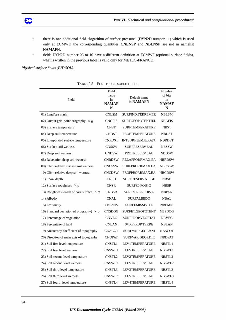
Part VI: ‘Technical and computational procedures’
sed
ds),
• there is one additional field “logarithm of surface pressure" (DYN2D number 11) which is u
only at ECMWF, the corresponding quantitiesCNLNSP and NBLNSP are not in namelist
NAMAFN .
• fields DYN2D number 06 to 10 have a different definition at ECMWF (optional surface fiel
what is written in the previous table is valid only for METEO-FRANCE.
Physical surface fields (PHYSOL):
TABLE 2.5 POST-PROCESSABLE FIELDS
Field
Fieldname
inNAMAF
N
Default namein NAMAFN
Numberof bits
inNAMAF
N
01) Land/sea mask CNLSM SURFIND.TERREMER NBLSM
02) Output grid-point orography CNGFIS SURFGEOPOTENTIEL NBGFIS
03) Surface temperature CNST SURFTEMPERATURE NBST
04) Deep soil temperature CNDST PROFTEMPERATURE NBDST
05) Interpolated surface temperature CNRDST INTSURFTEMPERATU NBRDST
06) Surface soil wetness CNSSW SURFRESERV.EAU NBSSW
07) Deep soil wetness CNDSW PROFRESERV.EAU NBDSW
08) Relaxation deep soil wetness CNRDSW RELAPROP.RMAX.EA NBRDSW
09) Clim. relative surface soil wetness CNCSSW SURFPROP.RMAX.EA NBCSSW
10) Clim. relative deep soil wetness CNCDSW PROFPROP.RMAX.EA NBCDSW
11) Snow depth CNSD SURFRESERV.NEIGE NBSD
12) Surface roughness CNSR SURFZ0.FOIS.G NBSR
13) Roughness length of bare surface CNBSR SURFZ0REL.FOIS.G NBBSR
14) Albedo CNAL SURFALBEDO NBAL
15) Emissivity CNEMIS SURFEMISSIVITE NBEMIS
16) Standard deviation of orography) CNSDOG SURFET.GEOPOTENT NBSDOG
17) Percentage of vegetation CNVEG SURFPROP.VEGETAT NBVEG
18) Percentage of land CNLAN SURFPROP.TERRE NBLAN
19) Anisotropy coefficient of topography CNACOT SURFVAR.GEOP.ANI NBACOT
20) Direction of main axis of topography CNDPAT SURFVAR.GEOP.DIR NBDPAT
21) Soil first level temperature CNSTL1 LEV1TEMPERATURE NBSTL1
22) Soil first level wetness CNSWL1 LEV1RESERV.EAU NBSWL1
23) Soil second level temperature CNSTL2 LEV2TEMPERATURE NBSTL2
24) Soil second level wetness CNSWL2 LEV2RESERV.EAU NBSWL2
25) Soil third level temperature CNSTL3 LEV3TEMPERATURE NBSTL3
26) Soil third level wetness CNSWL3 LEV3RESERV.EAU NBSWL3
27) Soil fourth level temperature CNSTL4 LEV4TEMPERATURE NBSTL4
g×
g×
g×
g×
94
IFS Documentation Cycle CY25r1 (Edited 2003)
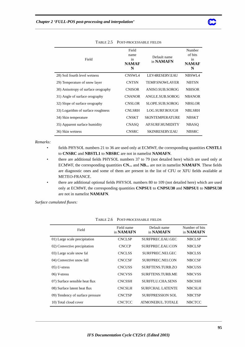
Chapter 2 ‘FULL-POS post-processing and interpolation’
nly at
le at
used
Remarks:
• fields PHYSOL numbers 21 to 36 are used only at ECMWF, the corresponding quantitiesCNSTL1to CNSRC andNBSTL1 to NBSRCare not in namelistNAMAFN .
• there are additional fields PHYSOL numbers 37 to 79 (not detailed here) which are used o
ECMWF, the corresponding quantitiesCN... andNB... are not in namelistNAMAFN . These fields
are diagnostic ones and some of them are present in the list of CFU or XFU fields availab
METEO-FRANCE.
• there are additional optional fields PHYSOL numbers 80 to 109 (not detailed here) which are
only at ECMWF, the corresponding quantitiesCNPSU1to CNPSU30andNBPSU1to NBPSU30are not in namelistNAMAFN .
Surface cumulated fluxes:
28) Soil fourth level wetness CNSWL4 LEV4RESERV.EAU NBSWL4
29) Temperature of snow layer CNTSN TEMP.SNOWLAYER NBTSN
30) Anisotropy of surface orography CNISOR ANISO.SUB.SOROG NBISOR
31) Angle of surface orography CNANOR ANGLE.SUB.SOROG NBANOR
32) Slope of surface orography CNSLOR SLOPE.SUB.SOROG NBSLOR
33) Logarithm of surface roughness CNLSRH LOG.SURF.ROUGH NBLSRH
34) Skin temperature CNSKT SKINTEMPERATURE NBSKT
35) Apparent surface humidity CNASQ AP.SURF.HUMIDITY NBASQ
36) Skin wetness CNSRC SKINRESERV.EAU NBSRC
TABLE 2.6 POST-PROCESSABLE FIELDS
FieldField name
in NAMAFNDefault name
in NAMAFNNumber of bitsin NAMAFN
01) Large scale precipitation CNCLSP SURFPREC.EAU.GEC NBCLSP
02) Convective precipitation CNCCP SURFPREC.EAU.CON NBCLSP
03) Large scale snow fal CNCLSS SURFPREC.NEI.GEC NBCLSS
04) Convective snow fall CNCCSF SURFPREC.NEI.CON NBCCSF
05)U-stress CNCUSS SURFTENS.TURB.ZO NBCUSS
06)V-stress CNCVSS SURFTENS.TURB.ME NBCVSS
07) Surface sensible heat flux CNCSSH SURFFLU.CHA.SENS NBCSSH
08) Surface latent heat flux CNCSLH SURFCHAL LATENTE NBCSLH
09) Tendency of surface pressure CNCTSP SURFPRESSION SOL NBCTSP
10) Total cloud cover CNCTCC ATMONEBUL.TOTALE NBCTCC
TABLE 2.5 POST-PROCESSABLE FIELDS
Field
Fieldname
inNAMAF
N
Default namein NAMAFN
Numberof bits
inNAMAF
N
95
IFS Documentation Cycle CY25r1 (Edited 2003)
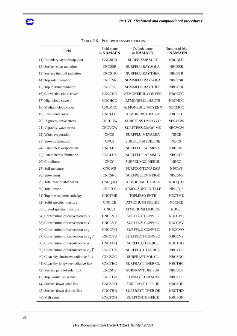
Part VI: ‘Technical and computational procedures’
11) Boundary layer dissipation CNCBLD SURFDISSIP SURF NBCBLD
12) Surface solar radiation CNCSSR SURFFLU.RAY.SOLA NBCSSR
13) Surface thermal radiation CNCSTR SURFFLU.RAY.THER NBCSTR
14) Top solar radiation CNCTSR SOMMFLU.RAY.SOLA NBCTSR
15) Top thermal radiation CNCTTR SOMMFLU.RAY.THER NBCTTR
16) Convective cloud cover CNCCCC ATMONEBUL.CONVEC NBCCCC
17) High cloud cover CNCHCC ATMONEBUL.HAUTE NBCHCC
18) Medium cloud cover CNCMCC ATMONEBUL.MOYENN NBCMCC
19) Low cloud cover CNCLCC ATMONEBUL.BASSE NBCLCC
20)U-gravity-wave stress CNCUGW SURFTENS.DMOG.ZO NBCUGW
21)V-gravity-wave stress CNCVGW SURFTENS.DMOG.ME NBCVGW
22) Water evaporation CNCE SURFFLU.MEVAP.EA NBCE
23) Snow sublimation CNCS SURFFLU.MSUBL.NE NBCS
24) Latent heat evaporation CNCLHE SURFFLU.LAT.MEVA NBCLHE
25) Latent heat sublimation CNCLHS SURFFLU.LAT.MSUB NBCLHS
26) Cloudiness CNCC SURFCUMUL NEBUL NBCC
27) Soil moisture CNCWS SURFCONTENU EAU NBCWS
28) Snow mass CNCSNS SURFRESERV NEIGE NBCSNS
29) Total precipitable water CNCQTO ATMOHUMI TOTALE NBCQTO
30) Total ozone CNCTO3 ATMOOZONE TOTALE NBCTO3
31) Top mesospheric enthalpy CNCTME TOPMESO ENTH NBCTME
32) Solid specific moisture CNCICE ATMOHUMI SOLIDE NBCICE
33) Liquid specific moisture CNCLI ATMOHUMI LIQUIDE NBCLI
34) Contribution of convection toU CNCCVU SURFFL.U CONVEC NBCCVU
35) Contribution of convection toV CNCCVV SURFFL.V CONVEC NBCCVV
36) Contribution of convection toq CNCCVQ SURFFL.Q CONVEC NBCCVQ
37) Contribution of convection to CNCCVS SURFFL.CT CONVEC NBCCVS
38) Contribution of turbulence toq CNCTUQ SURFFL.Q TURBUL NBCTUQ
39) Contribution of turbulence to CNCTUS SURFFL.CT TURBUL NBCTUS
40) Clear sky shortwave radiative flux CNCSOC SURFRAYT SOL CL NBCSOC
41) Clear sky longwave radiative flux CNCTHC SURFRAYT THER CL NBCTHC
42) Surface parallel solar flux CNCSOP SURFRAYT DIR SUR NBCSOP
43) Top parallel solar flux CNCTOP TOPRAYT DIR SOM NBCTOP
44) Surface down solar flux CNCSOD SURFRAYT DIFF DE NBCSOD
45) Surface down thermic flux CNCTHD SURFRAYT THER DE NBCTHD
46) Melt snow CNCFON SURFFONTE NEIGE NBCFON
TABLE 2.6 POST-PROCESSABLE FIELDS
FieldField name
in NAMAFNDefault name
in NAMAFNNumber of bitsin NAMAFN
cpT
cpT
96
IFS Documentation Cycle CY25r1 (Edited 2003)
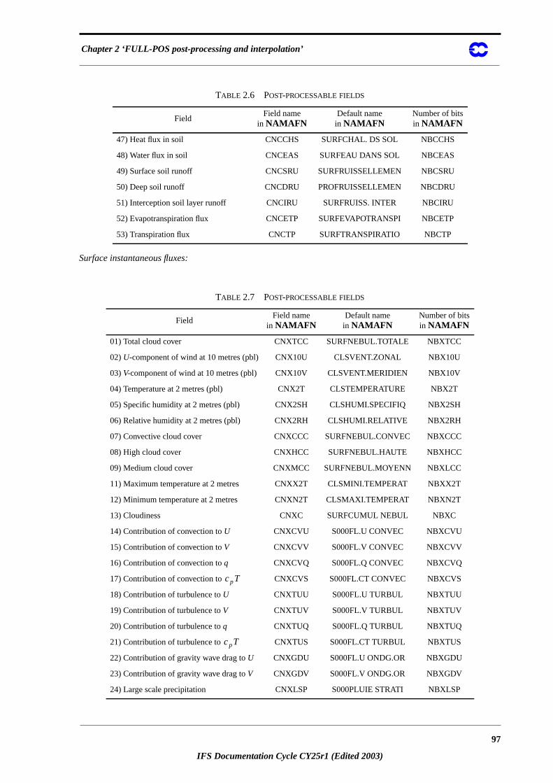
Chapter 2 ‘FULL-POS post-processing and interpolation’
Surface instantaneous fluxes:
47) Heat flux in soil CNCCHS SURFCHAL. DS SOL NBCCHS
48) Water flux in soil CNCEAS SURFEAU DANS SOL NBCEAS
49) Surface soil runoff CNCSRU SURFRUISSELLEMEN NBCSRU
50) Deep soil runoff CNCDRU PROFRUISSELLEMEN NBCDRU
51) Interception soil layer runoff CNCIRU SURFRUISS. INTER NBCIRU
52) Evapotranspiration flux CNCETP SURFEVAPOTRANSPI NBCETP
53) Transpiration flux CNCTP SURFTRANSPIRATIO NBCTP
TABLE 2.7 POST-PROCESSABLE FIELDS
FieldField name
in NAMAFNDefault name
in NAMAFNNumber of bitsin NAMAFN
01) Total cloud cover CNXTCC SURFNEBUL.TOTALE NBXTCC
02)U-component of wind at 10 metres (pbl) CNX10U CLSVENT.ZONAL NBX10U
03)V-component of wind at 10 metres (pbl) CNX10V CLSVENT.MERIDIEN NBX10V
04) Temperature at 2 metres (pbl) CNX2T CLSTEMPERATURE NBX2T
05) Specific humidity at 2 metres (pbl) CNX2SH CLSHUMI.SPECIFIQ NBX2SH
06) Relative humidity at 2 metres (pbl) CNX2RH CLSHUMI.RELATIVE NBX2RH
07) Convective cloud cover CNXCCC SURFNEBUL.CONVEC NBXCCC
08) High cloud cover CNXHCC SURFNEBUL.HAUTE NBXHCC
09) Medium cloud cover CNXMCC SURFNEBUL.MOYENN NBXLCC
11) Maximum temperature at 2 metres CNXX2T CLSMINI.TEMPERAT NBXX2T
12) Minimum temperature at 2 metres CNXN2T CLSMAXI.TEMPERAT NBXN2T
13) Cloudiness CNXC SURFCUMUL NEBUL NBXC
14) Contribution of convection toU CNXCVU S000FL.U CONVEC NBXCVU
15) Contribution of convection toV CNXCVV S000FL.V CONVEC NBXCVV
16) Contribution of convection toq CNXCVQ S000FL.Q CONVEC NBXCVQ
17) Contribution of convection to CNXCVS S000FL.CT CONVEC NBXCVS
18) Contribution of turbulence toU CNXTUU S000FL.U TURBUL NBXTUU
19) Contribution of turbulence toV CNXTUV S000FL.V TURBUL NBXTUV
20) Contribution of turbulence toq CNXTUQ S000FL.Q TURBUL NBXTUQ
21) Contribution of turbulence to CNXTUS S000FL.CT TURBUL NBXTUS
22) Contribution of gravity wave drag toU CNXGDU S000FL.U ONDG.OR NBXGDU
23) Contribution of gravity wave drag toV CNXGDV S000FL.V ONDG.OR NBXGDV
24) Large scale precipitation CNXLSP S000PLUIE STRATI NBXLSP
TABLE 2.6 POST-PROCESSABLE FIELDS
FieldField name
in NAMAFNDefault name
in NAMAFNNumber of bitsin NAMAFN
cpT
cpT
97
IFS Documentation Cycle CY25r1 (Edited 2003)
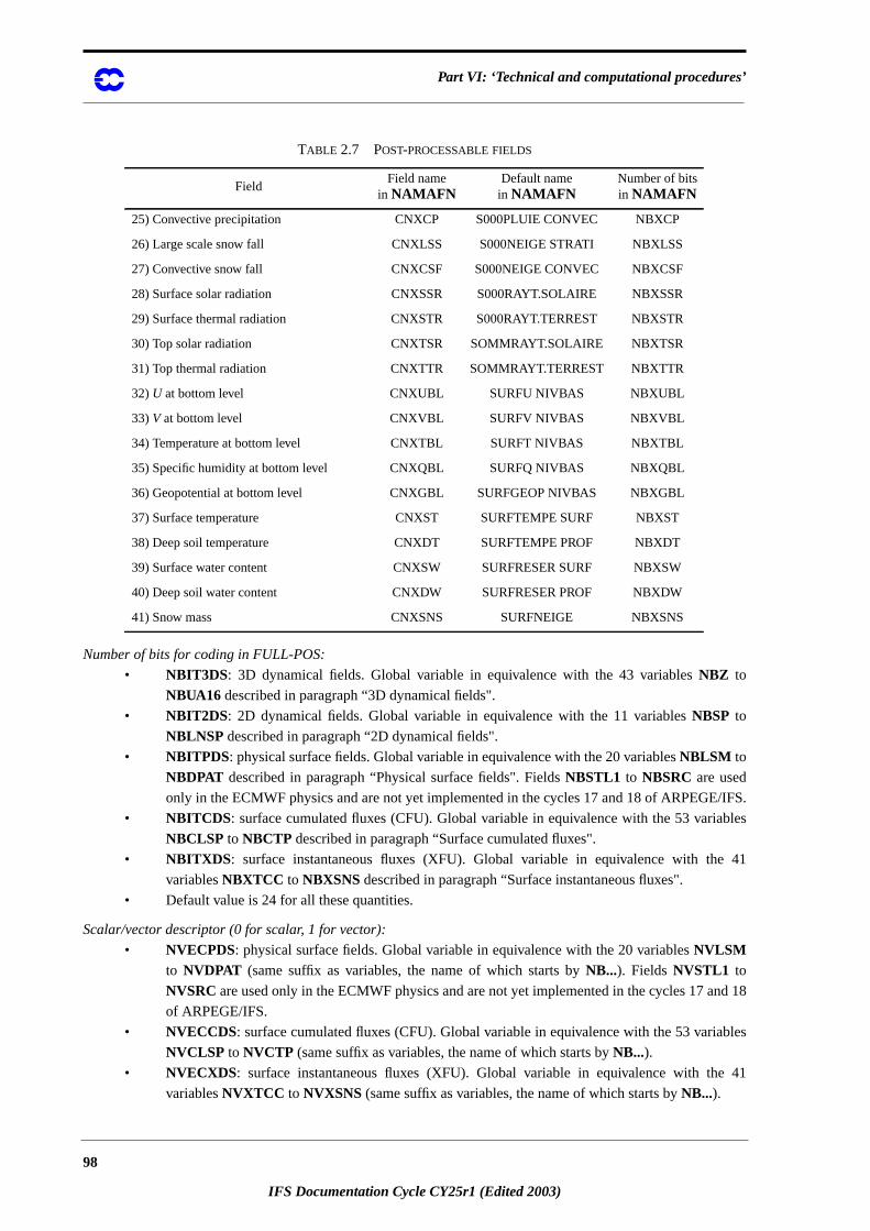
Part VI: ‘Technical and computational procedures’
/IFS.
bles
41
d 18
bles
41
Number of bits for coding in FULL-POS:
• NBIT3DS: 3D dynamical fields. Global variable in equivalence with the 43 variablesNBZ to
NBUA16 described in paragraph “3D dynamical fields".
• NBIT2DS: 2D dynamical fields. Global variable in equivalence with the 11 variablesNBSP to
NBLNSP described in paragraph “2D dynamical fields".
• NBITPDS: physical surface fields. Global variable in equivalence with the 20 variablesNBLSM to
NBDPAT described in paragraph “Physical surface fields". FieldsNBSTL1 to NBSRC are used
only in the ECMWF physics and are not yet implemented in the cycles 17 and 18 of ARPEGE
• NBITCDS: surface cumulated fluxes (CFU). Global variable in equivalence with the 53 varia
NBCLSP to NBCTP described in paragraph “Surface cumulated fluxes".
• NBITXDS : surface instantaneous fluxes (XFU). Global variable in equivalence with the
variablesNBXTCC to NBXSNS described in paragraph “Surface instantaneous fluxes".
• Default value is 24 for all these quantities.
Scalar/vector descriptor (0 for scalar, 1 for vector):
• NVECPDS: physical surface fields. Global variable in equivalence with the 20 variablesNVLSMto NVDPAT (same suffix as variables, the name of which starts byNB...). Fields NVSTL1 to
NVSRC are used only in the ECMWF physics and are not yet implemented in the cycles 17 an
of ARPEGE/IFS.
• NVECCDS: surface cumulated fluxes (CFU). Global variable in equivalence with the 53 varia
NVCLSP to NVCTP (same suffix as variables, the name of which starts byNB...).• NVECXDS: surface instantaneous fluxes (XFU). Global variable in equivalence with the
variablesNVXTCC to NVXSNS (same suffix as variables, the name of which starts byNB...).
25) Convective precipitation CNXCP S000PLUIE CONVEC NBXCP
26) Large scale snow fall CNXLSS S000NEIGE STRATI NBXLSS
27) Convective snow fall CNXCSF S000NEIGE CONVEC NBXCSF
28) Surface solar radiation CNXSSR S000RAYT.SOLAIRE NBXSSR
29) Surface thermal radiation CNXSTR S000RAYT.TERREST NBXSTR
30) Top solar radiation CNXTSR SOMMRAYT.SOLAIRE NBXTSR
31) Top thermal radiation CNXTTR SOMMRAYT.TERREST NBXTTR
32)U at bottom level CNXUBL SURFU NIVBAS NBXUBL
33)V at bottom level CNXVBL SURFV NIVBAS NBXVBL
34) Temperature at bottom level CNXTBL SURFT NIVBAS NBXTBL
35) Specific humidity at bottom level CNXQBL SURFQ NIVBAS NBXQBL
36) Geopotential at bottom level CNXGBL SURFGEOP NIVBAS NBXGBL
37) Surface temperature CNXST SURFTEMPE SURF NBXST
38) Deep soil temperature CNXDT SURFTEMPE PROF NBXDT
39) Surface water content CNXSW SURFRESER SURF NBXSW
40) Deep soil water content CNXDW SURFRESER PROF NBXDW
41) Snow mass CNXSNS SURFNEIGE NBXSNS
TABLE 2.7 POST-PROCESSABLE FIELDS
FieldField name
in NAMAFNDefault name
in NAMAFNNumber of bitsin NAMAFN
98
IFS Documentation Cycle CY25r1 (Edited 2003)
Chapter 2 ‘FULL-POS post-processing and interpolation’
18 of
bles
41
• Default value is 1 forNVCUSS, NVCVSS, NVCUGW, NVCVGW, NVX10U, NVX10V, 0 for the
other quantities.
Use of land-sea mask for horizontal interpolations (0=no; 1=yes):
• NITMPDS : physical surface fields. Global variable in equivalence with the 20 variablesNILSM to
NIDPAT (same suffix as variables, the name of which starts byNB...). FieldsNISTL1 to NISRCare used only in the ECMWF physics and are not yet implemented in the cycles 17 and
ARPEGE/IFS.
• NITMCDS : surface cumulated fluxes (CFU). Global variable in equivalence with the 53 varia
NICLSP to NICTP (same suffix as variables, the name of which starts byNB...).• NITMXDS : surface instantaneous fluxes (XFU). Global variable in equivalence with the
variablesNIXTCC to NIXSNS (same suffix as variables, the name of which starts byNB...).• Default value is 0 forNILSM , NIGFIS , NISDOG, 1 for the other physical surface fields
quantities, 1 forNICUSS, NICVSS, NICUGW, NICVGW , NIX10U, NIX10V, NIX2T , NIX2SH,
NIX2RH , NIXX2T , NIXN2T , 0 for the other CFU or XFU quantities.
Namelist NAMAFN:
The following variables ofYOMAFN are in namelistNAMAFN : CNZ, CNT, CNU, CNV, CNQ, CNR, CNS,
CNVV, CNVOR, CNDIV, CNTH , CNPSI, CNKHI , CNW, CNTPW, CNCLF, CNWND, CNETH , CNABS,
CNSTD, CNSHD, CNPV, CNWPV, CNSCVA, CNP, CNUA1, CNUA2, CNUA3, CNSP, CNMSL , CNFIS,
CNGM , CNFOL , CNSU1, CNSU2, CNSU3, CNSU4, CNSU5, CNLSM , CNGFIS, CNST, CNDST, CNRDST,
CNSSW, CNDSW, CNRDSW, CNCSSW, CNCDSW, CNSD, CNSR, CNBSR, CNAL , CNEMIS , CNSDOG,
CNVEG, CNLAN , CNACOT, CNDPAT, CNCLSP, CNCCP, CNCLSS, CNCCSF, CNCUSS, CNCVSS, CNC-SSH, CNCSLH, CNCTSP, CNCTCC, CNCBLD , CNCSSR, CNCSTR, CNCTSR, CNCTTR , CNCCCC,
CNCHCC, CNCMCC , CNCLCC , CNCUGW, CNCVGW, CNCE, CNCS, CNCLHE , CNCLHS, CNCC,
CNCWS, CNCSNS, CNCQTO, CNCTO3, CNCTME , CNCICE , CNCLI , CNCCVU, CNCCVV, CNCCVQ,
CNCCVS, CNCTUQ, CNCTUS, CNCSOC, CNCTHC , CNCSOP, CNCTOP, CNCSOD, CNCTHD , CNC-FON, CNCCHS, CNCEAS, CNCSRU, CNCDRU, CNCIRU , CNCETP, CNCTP, CNXTCC , CNX10U,
CNX10V, CNX2T, CNX2SH, CNX2RH, CNXCCC, CNXHCC , CNXMCC , CNXLCC , CNXX2T, CNXN2T,
CNXC, CNXCVU , CNXCVV, CNXCVQ , CNXCVS, CNXTUU , CNXTUV, CNXTUQ , CNXTUS,
CNXGDU, CNXGDV, CNXLSP, CNXCP, CNXLSS, CNXCSF, CNXSSR, CNXSTR, CNXTSR, CNXTTR ,
CNXUBL , CNXVBL , CNXTBL , CNXQBL , CNXGBL , CNXST, CNXDT, CNXSW, CNXDW, CNXSNS,
NBZ, NBT, NBU, NBV, NBQ, NBR, NBS, NBVV, NBVOR, NBDIV, NBTH , NBPSI, NBKHI , NBW, NBTPW,
NBCLF, NBWND, NBETH , NBABS, NBSTD, NBSHD, NBPV, NBWPV, NBSCVA, NBP, NBUA1, NBUA2,
NBUA3, NBSP, NBMSL , NBFIS, NBGM , NBFOL , NBSU1, NBSU2, NBSU3, NBSU4, NBSU5, NBLSM , NB-GFIS, NBST, NBDST, NBRDST, NBSSW, NBDSW, NBRDSW, NBCSSW, NBCDSW, NBSD, NBSR, NBB-SR, NBAL , NBEMIS , NBSDOG, NBVEG, NBLAN , NBACOT, NBDPAT, NBCLSP, NBCCP, NBCLSS,
NBCCSF, NBCUSS, NBCVSS, NBCSSH, NBCSLH, NBCTSP, NBCTCC, NBCBLD , NBCSSR, NBCSTR,
NBCTSR, NBCTTR , NBCCCC, NBCHCC, NBCMCC , NBCLCC , NBCUGW, NBCVGW, NBCE, NBCS,
NBCLHE , NBCLHS, NBCC, NBCWS, NBCSNS, NBCQTO, NBCTO3, NBCTME , NBCICE , NBCLI ,
NBCCVU, NBCCVV, NBCCVQ, NBCCVS, NBCTUQ, NBCTUS, NBCSOC, NBCTHC , NBCSOP, NBC-TOP, NBCSOD, NBCTHD , NBCFON, NBCCHS, NBCEAS, NBCSRU, NBCDRU, NBCIRU , NBCETP,
NBCTP, NBXTCC , NBX10U, NBX10V, NBX2T, NBX2SH, NBX2RH, NBXCCC, NBXHCC , NBXMCC ,
NBXLCC , NBXX2T, NBXN2T, NBXC, NBXCVU , NBXCVV, NBXCVQ , NBXCVS, NBXTUU , NBXTUV,
NBXTUQ , NBXTUS, NBXGDU, NBXGDV, NBXLSP, NBXCP, NBXLSS, NBXCSF, NBXSSR, NBXSTR,
NBXTSR, NBXTTR , NBXUBL , NBXVBL , NBXTBL , NBXQBL , NBXGBL , NBXST, NBXDT, NBXSW,
NBXDW, NBXSNS, NILSM , NIGFIS , NIST, NIDST, NIRDST, NISSW, NIDSW, NIRDSW, NICSSW,
99
IFS Documentation Cycle CY25r1 (Edited 2003)
Part VI: ‘Technical and computational procedures’
tine
are in-
on
NICDSW, NISD, NISR, NIBSR, NIAL , NIEMIS , NISDOG, NIVEG , NILAN , NIACOT , NIDPAT .
2.12.4 YOMAFPB.
Contains buffer for basic fields resulting from APACHE in FULL-POS. Variables are initialised in setup rou
setup/SUFPSC2B. No variable in namelist. All variables are DM-local.
List of variables:
• NLENAFPBL : length of buffer.
• AFPBUF : buffer.
• NSTAAFPB : start adresses for post-processed packets of points within buffer.
2.12.5 YOMAFPDS.
Absolute pointers of the basic fields which have been horizontally then vertically post-processed. Variables
itialised in setup routinesetup/SUAFPDS. No variable in namelist. All variables are DM-global.
Field pointers:
• MFPUPT2: for upper air pressure.
• MFPAPT2: for cloud fraction.
• MFPUT2 : for zonal component of wind.
• MFPVT2 : for meridian component of wind.
• MFPTT2 : for temperature.
• MFPQT2 : for specific humidity.
• MFPWT2 : for liquid water.
• MFPST2 : for ice.
• MFPSVT2: for passive scalar variables.
• MFPSPT2: for surface pressure.
Other variables:
• NAFPOS : number of fields.
• NFPALEV : maximum number of fields.
2.12.6 YOMCT0.
Contains control variables. The following variables also present in namelistNAMCT0 can be useful for FULL-
POS (these variables are DM-global).
• NCONF: configuration (default value is 1).
• LFPOS: FULL-POS main switch (default value is .FALSE.).
• NFRPOS: post-processing frequency (default value depends on configuration).
• NPOSTS: post-processing control array (default value depends on configuration).
• LIOGAUX : I/O on unfitted vertically post-processed fields (default value depends
configuration).
• LIOFOU1 : I/O on Fourier data (default value depends on configuration).
• LIOLPOL : I/O on Legendre polynomial (default value depends on configuration).
• LIOSPEC: I/O on saved spectral data (default value depends on configuration).
• LIOSUA : I/O on saved upper air grid-point data (default value depends on configuration).
• LIOSSU: I/O on saved surface data (default value depends on configuration).
• LIOSCF : I/O on saved cumulated fluxes data (default value depends on configuration).
• LIOSXF : I/O on saved instantaneous fluxes data (default value depends on configuration).
100
IFS Documentation Cycle CY25r1 (Edited 2003)
Chapter 2 ‘FULL-POS post-processing and interpolation’
-
uth
est
ace.
uth
me as
tion.
lue
bal).
-
• LMLTSK : switch for multitasking (default value depends on configuration).
• NTASKS: number of processors (default value depends on configuration).
• CNPPATH: path name for selection files (default value is ’ ’).
• CFPNCF: file name for FULL-POS control file (default value is ’ncf927’).
The following variables also present in namelistNAMPAR0 can be useful for FULL-POS when running distrib
uted memory jobs (these variables are DM-global).
• NPRGPNS: number of processors used in A-direction during grid-point phase in North-So
direction.
• NPRGPEW: number of processors used in B-direction during grid-point phase in East-W
direction.
• NPRTRW: number of processors used in A-direction during transform phase in wave sp
Default value is the same asNPRGPNS.
• NPRTRNS: number of processors used in A-direction during transform phase in North-So
direction ( used to dimension some arrays used in Fourier transforms). Default value is the sa
NPRGPNS.
• NPRTRV: number of processors used in B-direction during transform phase in vertical direc
Default value is the same asNPRTREW.
• NPROCK: not currently used.
• NPROC: total number of processors requested (DM-global).NPROC has to be equal to the
productsNPROCA*NPROCB, NPRGPNS*NPRGPEW, NPRTRW*NPRTRV. Default value is
1 for distributed memory, 0 for shared memory.
• NOUTPUT: type of output (DM-global).
• 0 = no diagnostic output;
• 1 = only diagnostic output from processor number 1.
• 2 = diagnostic output from all processors into separate files.
Default value is 1.
• LMESSP: .TRUE./.FALSE.: distributed memory/ shared memory run (DM-global). Default va
is .FALSE. .
• LMPDIAG : extensive message passing diagnostic output requested if .TRUE. (DM-glo
Default value is .FALSE. .
The following variables also present in namelistNAMPAR1 can be useful for FULL-POS when running distrib
uted memory jobs (these variables are DM-global). They are read and initialised insetup/SUMP0.
• NINSTR1: number of time steps instrumented (DM-global). Default value is 0.
• NINSTR2: number of time steps instrumented (DM-global). Default value is 0.
2.12.7 YOMDFPB.
Contains buffer for fully post-processed dynamical fields. Variables are initialised in setup routinesetup/SUFPSC2B. No variable in namelist. All variables are DM-local.
List of variables:
• NLENDFPBL : length of buffer.
• GDFPBUF : buffer.
• NSTADFPB : start adresses for post-processed packets of points within buffer.
101
IFS Documentation Cycle CY25r1 (Edited 2003)
Part VI: ‘Technical and computational procedures’
lue
al).
al).
one
the
tted
ted,
tted
iven
dre
dre
utine
2.12.8 YOMDIM.
Contains dimensioning variables. The following variables are related with FULL-POS.
Variables computed in SUDIM:
• NDLON : maximum number of Gaussian/Lobatto longitudes (DM-global).
• NFPXLEV : maximum number of post-processing levels (DM-global).
• NPMAX : post-processing truncation (DM-global, default value is generallyNSMAX ).
• NFPPHYB: maximum number of post-processed physical fields (DM-global).
• NPROMA : working dimension of (vertical) post-processing rows (DM-global, default va
depends on configuration).
• NGPBLKS: number ofNPROMA -subpackets in a processor (DM-local).
• NDGSAFPH: modified lower bound for latitude (DM-local).
• NDGENFPH: modified upper bound for latitude (DM-local).
Variables computed under SUFPDIM:
• NFPGT1: maximum number of fields to be vertically post-processed (DM-global).
• NFPAUXB: maximum number of vertically post-processed fields to remain unfitted (DM-glob
• NFPSPA: maximum number of underived vertically post-processed fields to be fitted (DM-glob
• NFPSPD: maximum number of derived vertically post-processed fields to be fitted, given
horizontal subdomain (DM-global).
• NFPSPB: maximum number of derived vertically post-processed fields to be fitted, given
maximum number of horizontal subdomains (DM-global).
• NFPGT0B: maximum number of fields to be horizontally post-processed (DM-global).
• NFPDYNB: maximum number of post-processed dynamical fields (DM-global).
• NFPAVEC: maximum number of vectorial underived vertically post-processed fields to be fi
(DM-global).
• NFPBVEC: maximum number of vectorial derived vertically post-processed fields to be fit
given the maximum number of horizontal subdomains (DM-global).
• NFPASCA: maximum number of scalar underived vertically post-processed fields to be fi
(DM-global).
• NFPBSCA: maximum number of scalar derived vertically post-processed fields to be fitted, g
the maximum number of horizontal subdomains (DM-global).
• NFPLEI : maximum number of useful fields in the working arrays for the inverse Legen
transforms (DM-global).
• NFPLED: maximum number of useful fields in the working arrays for the direct Legen
transforms on wind (DM-global).
Namelist NAMDIM:
The following variables ofYOMDIM are in namelistNAMDIM : NPROMA , NPMAX .
2.12.9 YOMFP4.
Contains dimensions for FULL-POS on one-level-type dynamical fields. Variables are initialised in setup ro
setup/SU4FPOS. No variable in namelist. All variables are DM-global.
Number of fields in each array/buffer for dynamics:
• NGT1FP : number of fields inGT1 (fields to be fitted).
• NAUXFPB: number of fields inGAUXBUF (fields to remain unfitted).
• NAUX3FP: number of 3D fields inGAUXBUF (fields to remain unfitted).
102
IFS Documentation Cycle CY25r1 (Edited 2003)
Chapter 2 ‘FULL-POS post-processing and interpolation’
ion
tialised
• NSPAFP: number of useful fields inSPAFP.• NSPBFP: number of useful fields inSPBFP.• NSPDFP: number of useful fields inSPDFP.• NGT0FPB: number of fields inGT0BUF during an horizontal post-processing time step.
• NGT03FP: number of 3D fields inGT0BUF during an horizontal post-processing time step.
• NDYNFPB: number of fields inGDFPBUF.
Dimensions for dynamical fields post-processing:
• NOFP3F : total number of 3D fields.
• NOFP3A : total number of subdomains for each level of each field. Array of dimens
(NFPXLEV,NFP3DF).
• NOFPLEV: total number of levels for each field. Array of dimensionNFP3DF.
• NAVECFP: number of vectorial underived vertically post-processed fields to be fitted.
• NBVECFP: number of vectorial derived vertically post-processed fields to be fitted.
• NASCAFP: number of scalar underived vertically post-processed fields to be fitted.
• NBSCAFP: number of scalar derived vertically post-processed fields to be fitted.
• NLEIFP : number of fields in the working arrays for the inverse Legendre transforms.
• NLEDFP : number of fields in the working arrays for the direct Legendre transforms.
Dimensions for physical fields and fluxes post-processing:
• NPHYFPB: number of physical fields.
• NCFUFPB: number of cumulated fluxes.
• NXFUFPB: number of instantaneous fluxes.
2.12.10 YOMFP4L.
Contains information relative to lagged variables needed to write out post-processed fields. Variables are ini
in the sequencepp_obs/DYNFPOS setup/SUVFPOSL. No variable in namelist. All variables are DM-glo-
bal.
Horizontally post-processed dynamical variables:
• NDYNFPL : number of fields inGDFPBUF.
• NFLDFPL : field pointer. Array of dimensionNFPDYNB.
• RLEVFPL : level value. Array of dimensionNFPDYNB.
• NBITFPL : number of bits when writing output file. Array of dimensionNFPDYNB.
• NDOMFPL : number of subdomains for each field. Array of dimensionNFPDYNB.
• NINDFPL : indices of subdomains for each field. Array of dimension (NFPDOM,NFPDYNB).
• NAUXFPL : number of fields inGAUXBUF (fields to remain unfitted).
• NAUX3FPL : number of 3D fields inGAUXBUF (fields to remain unfitted).
• NGT0FPL : number of fields inGT0BUF during an horizontal post-processing time step.
• NGT03FPL: number of 3D fields inGT0BUF during an horizontal post-processing time step.
Spectral variables:
• NSPAFPL : number of fields inSPAFP.• NSPDFPL : number of fields inSPDFP.• NFLDAFPL : field pointers inSPAFP. Array of dimensionNFPSPA.
• NFLDDFPL : field pointers inSPDFP. Array of dimensionNFPSPD.
• RLEVAFPL : level values inSPAFP. Array of dimensionNFPSPA.
• RLEVDFPL : level values inSPDFP. Array of dimensionNFPSPD.
→
103
IFS Documentation Cycle CY25r1 (Edited 2003)
Part VI: ‘Technical and computational procedures’
s. If
sted,
e at
t-
e at
t-
mum
ve at
t-
have
to
ly
WF
WF
ly).
MWF
Grid-point variables:
• NFLDFPXL : field pointers inGAUXBUF. Array of dimensionNFPAUXB.
• RLEVFPXL : level values inGAUXBUF. Array of dimensionNFPAUXB.
• NBITFPXL : number of bit when writing outGAUXBUF. Array of dimensionNFPAUXB.
2.12.11 YOMFPC.
Contains scientific and technical variables for post-processing. Variables are initialised in setup routinesetup/SUF-PC. All variables are DM-global.
Technical variables.
• CFPDIR: prefix (path) for the output files (default value is ’PF’).
• CFPIDEN: identificator of the output files.
• CFPFMT: format of the output files, can take the following values:
• ’MODEL’ for output in spherical harmonics.
• ’GAUSS’ for output in grid-point space on Gaussian grid (covering the global sphere).
• ’LELAM’ for output on a grid of kind ’ALADIN’ (spectral or grid-point coefficients).
• ’LALON’ for a grid of kind “latitudes * longitudes’.
Default is ’GAUSS’ in ARPEGE/IFS, ’LELAM’ in ALADIN.
• CFPDOM, C1FPDOM: names of the subdomains. Names have at maximum 7 character
CFPFMT = ’GAUSS’ or ’LELAM’ only one output domain is allowed. IfCFPFMT = ’LALON’
the maximum of output subdomains allowed is 10. By default, one output domain is reque
CFPDOM(1)=’000’ andCFPDOM(i)=” for i>1.
• CFP3DF, C1FP3DF: names of the 3D dynamics fields to be post-processed. Names hav
maximum 12 characters. By defaultCFP3DF contains blanks (no 3D dynamical field to pos
process).
• CFP2DF, C1FP2DF: names of the 2D dynamics fields to be post-processed. Names hav
maximum 16 characters. By defaultCFP2DF contains blanks (no 2D dynamical field to pos
process).
• CFPPHY, C1FPPHY: names of the physical fields to be post-processed. Names have at maxi
16 characters. By defaultCFPPHY contains blanks (no physical field to post-process).
• CFPCFU, C1FPCFU: names of the cumulated fluxes fields to be post-processed. Names ha
maximum 16 characters. By defaultCFPCFU contains blanks (no cumulated fluxes field to pos
process).
• CFPXFU, C1FPXFU: names of the instantaneous fluxes fields to be post-processed. Names
at maximum 16 characters. By defaultCFPXFU contains blanks (no instantaneous fluxes field
post-process).
• remark: variablesCFP(XXX) andC1FP(XXX) are in equivalence (same quantity) but different
dimensioned.
• MFP3DF: gribcodes of the 3D dynamics fields to be post-processed (variable used at ECM
only).
• MFP2DF: gribcodes of the 2D dynamics fields to be post-processed (variable used at ECM
only).
• MFPPHY: gribcodes of the physical fields to be post-processed (variable used at ECMWF on
• MFPCFU: gribcodes of the cumulated fluxes fields to be post-processed (variable used at EC
only).
104
IFS Documentation Cycle CY25r1 (Edited 2003)
Chapter 2 ‘FULL-POS post-processing and interpolation’
ed at
lue is
t
lt
al
al
al
ost-
ept if
.T. .
value
.F. .
. .
ind
ct to
nd the
• MFPXFU : gribcodes of the instantaneous fluxes fields to be post-processed (variable us
ECMWF only).
• RFP3P: list of post-processing pressure levels in Pa (no default value).
• RFP3H: list of post-processing height (above orography) levels in meters (no default value).
• RFP3TH: list of post-processing potential temperature levels in Kelvins (no default value).
• RFP3PV: list of post-processing potential vorticity levels in S.I. units (no default value).
• NRFP3S: list of post-processing -levels (pseudo-configuration 927 only). No default value.
• LFPCNT: control varying output variables according to time step.
• LFPNORM : print out the mean of each post-processed field for each subdomain (default va
.TRUE.).
• LTRACEFP : trace for FULL-POS (additional prints on listing, default value is .FALSE.).
• NFPGRIB: level of GRIB coding in output file ARPEGE/ALADIN for grid-point arrays (defaul
value is 2).
• NFPGRSP: level of GRIB coding in output file ARPEGE/ALADIN for spectral arrays (defau
value is 2).
• LFPBACK : .TRUE. to return to initial geometry (caseLFPSPEC) (default value is .FALSE.).
• NFPDOM: useful dimension ofCFPDOM.
• NFP3DF: useful dimension ofCFP3DF (default value is the number of 3D wanted dynamic
fields).
• NFP2DF: useful dimension ofCFP2DF (default value is the number of 2D wanted dynamic
fields).
• NFPPHY: useful dimension ofCFPPHY (default value is the number of wanted surface physic
fields).
• NFPCFU: useful dimension ofCFPCFU.
• NFPXFU: useful dimension ofCFPXFU.
• NFP3P: useful dimension ofRFP3P.• NFP3H: useful dimension ofRFP3H.
• NFP3TH: useful dimension ofRFP3TH.
• NFP3PV: useful dimension ofRFP3PV.
• NFP3S: useful dimension ofNRFP3S.
Scientific variables.
• LFPSPEC: .T. if post-processed dynamical fields are written out as spectral coefficients, .F. if p
processed dynamical fields are written out as grid point values (default value is .FALSE., exc
second part of a pseudo-configuration 927 or E927).
• LFIT2D : 1 if 2D dynamical post-processed fields should be fitted, 0 otherwise. Default value is
• LFITP : .T. if post-processed fields on pressure levels should be fitted, .F. otherwise. Default
is .T. .
• LFITH : .T. if post-processed fields on height levels should be fitted, .F. otherwise.
• LFITT : .T. if post-processed fields on -levels should be fitted, .F. otherwise. Default value is
• LFITV : .T. if post-processed fields onPV-levels should be fitted, .F. otherwise. Default value is .F
• LFITS : .T. if post-processed fields on -levels should be fitted, .F. otherwise.
• LFPUVDZ : .T. if divergence and vorticity should be post-processed with respect to the w
components (default value is .TRUE.).
• LFPUVKP : .T. if stream function and potential velocity should be post-processed with respe
the wind components, otherwise they are post-processed with respect to the divergence a
vorticity (default value is .TRUE.).
η
θ
η
105
IFS Documentation Cycle CY25r1 (Edited 2003)
Part VI: ‘Technical and computational procedures’
ernal
le
st-
sk,
elative
ge of
main
first
amed
sest
ain,
ve
r to
nt of
d to
ntity.
dard
tput
• NFPCLI : usage level for climatology:
• 0: no climatology (default value).
• 1: orography and land-sea mask of output only. In your script, the local name of this ext
climatology file should be “const.clim.DDDDDDD", where DDDDDDD is the variab
CFPDOM of the namelistNAMFPC . This file should be of the same geometry as the po
processing file you want to make.
• 2: all available climatological fields of the current month. Use of auxiliary land-sea ma
orography, surface temperature, relative surface wetness, deep soil temperature, r
deep soil wetness, albedo, emissivity, standard deviation of orography, percenta
vegetation, roughness length, anisotropy coefficient of topography, direction of the
axis of topography and snow depth. For that you need to make 2 climatology files: the
one, named “Const.Clim", should be in the input model geometry, the second one, n
“const.clim.DDDDDDD", where DDDDDDD is the variableCFPDOM of the namelist
NAMFPC , should be in the output (post-processing) geometry.
• 3: shifting mean from the climatological fields of the current month to the ones of the clo
month.
• NDOMFP: domain definition of fields in files;NDOMFP = 1: physical fields are grid-points stored
on (C+I)+E and dynamical fields are spectral (option available in ALADIN only);NDOMFP = -1:
physical and dynamical fields are grid-points stored on (C+I)+E;NDOMFP = 0: physical and
dynamical fields are grid-points stored on (C+I). C, I, E mean respectively conservation dom
intermediate zone and extension zone. Default value depends on configuration:
• if CFPFMT=’MODEL’, LFPSPEC=.F., default value is -1.
• if CFPFMT=’GAUSS’,’LELAM’ or ’LALON’ and LFPSPEC=.F., default value is 0.
• if CFPFMT=’GAUSS’ or ’LELAM’ and LFPSPEC=.T., default value is -1 for the first
part, 1 for the second part.
• LFPQ: .T. if specific humidity is interpolated (then deduct relative humidity), .F. if relati
humidity is interpolated (then deduct specific humidity). Default value is .FALSE. . It is bette
use the default value (.FALSE.): in this case, relative humidity is conserved within displaceme
the planetary boundary layer and it is interpolated vertically. Relative humidity is considere
have better properties for an interpolation than mixing ratio even if it is not a conservative qua
• LASQ: .T. if apparent surface humidity is set to 80% saturation (default value is .FALSE.).
• WSXI : maximum surface moisture in input.
• WDXI : maximum deep soil moisture in input.
• WSXO: maximum surface moisture in output. Default value is -999. .
• WDXO : maximum deep soil moisture in output. Default value is -999. .
• WCXO : maximum “climatological" moisture in output. Default value is -999. .
• LSNOWI : snow in the input file. Default value is equal toLNEIGE .
• LSNOWO: snow in the output file. Default value is equal toLNEIGE .
• FPBL: critical thickness of PBL. Default value is 17500 Pa.
• RFPCORR: critical orography difference for correcting surface temperature through stan
profile, in J/kg. Default value is 300*g.
• RFPMXZ : non-critical maximum difference between interpolated orography and ou
orography, in J/kg. Default value is 3000*g.
• LFPSPLIT : .TRUE. if split of FULL-POS post-processing of dynamical fields.
• NFPSPLIT: number of dynamical fields to be post-processed at a time.
• MFP3DYN : maximum number of 3D-dynamical fields needed forLFPART2 .
• MFP2DYN : maximum number of 2D-dynamical fields needed forLFPART2 .
106
IFS Documentation Cycle CY25r1 (Edited 2003)
Chapter 2 ‘FULL-POS post-processing and interpolation’
del,
witch
ls, it
before
.
are ini-
id is
o the
.
.
al).
l).
s of
unt,
o be
of
• NFPTRSPLIT: pointer to actual post-processing package of dynamical fields.
Remarks.
• Note that if you ask for post-processing of dynamical fields which are not spectral in the mo
then these post-processed fields will not be spectrally fitted, even if the corresponding s
LFIT... is .TRUE. .
• Note that if you wish to post-process upper air dynamical fields on height levels or hybrid leve
is not possible to apply such spectral fit because the horizontal interpolations are performed
the vertical interpolation in order to respect the displacement of the planetary boundary layer
Namelist NAMFPC:
The following variables ofYOMFPC are in namelistNAMFPC : CFPDIR, CFPFMT, CFPDOM, CFP3DF,
CFP2DF, CFPPHY, CFPCFU, CFPXFU, LFPSPEC, LFPBACK , RFP3P, RFP3H, RFP3TH, RFP3PV,
NRFP3S, NFPGRIB, NFPGRSP, NDOMFP, LFIT2D , LFITP , LFITT , LFITV , LFITS , RFPCORR, LFPU-VDZ , LFPUVKP, NFPCLI , LFPQ, WSXO, WDXO , WCXO , LSNOWI , LSNOWO, LFPNORM , LTRACE-FP, FPBL, RFPMXZ , LASQ, MFP3DF, MFP2DF, MFPPHY, NFP3DF, NFP2DF, NFPPHY, LFPSPLIT ,
NFPSPLIT.
2.12.12 YOMFPD.
Variables concerning the boundaries and the horizontal dimensions of each output subdomain. Variables
tialised in setup routinesetup/SUFPD.
For all kinds of output (sub)domains:
• NLAT : number of latitudes for each output (sub)domain (poles not included if a Gaussian gr
required); array of integers; corresponds to the variableNDGLG of the output grid(s) (DM-global).
• NLON : number of longitudes for each output (sub)domain; array of integers; corresponds t
variableNDLON of the output grid(s) (DM-global).
• RLATN : northern latitude in degrees for each output (sub)domain; array of reals (DM-global)
• RLATS : southern latitude in degrees for each output (sub)domain; array of reals (DM-global)
• RLONW : western longitude in degrees for each output (sub)domain; array of reals (DM-glob
• RLONE : eastern longitude in degrees for each output (sub)domain; array of reals (DM-globa
• NFPSIZEG: number of points in each subdomain (DM-global).
• NFPSIZEL : DM-local version of variableNFPSIZEG, its value is computed inSUFPG.
• NFPGP: maximum number of output points (DM-global). This is the sum on all the subdomain
theNFPSIZEG. Reduction of the grid near the poles for global output grids is not taken in acco
soNFPSIZEG can be above the actual total number of points where interpolations will have t
done.
• NFPD1: first dimension of the array to be written on output file (DM-global).NFPD1can be above
NFPGP for global domains (NFPD1 counts polar latitudes contrary toNFPGP) and ALADIN
domains (NFPD1 can count extension zone points according to the value ofNDOMFP in
NAMFPC butNFPGP does not count any point of the extension zone).
These variables have many possible default values, according to the content of the namelistNAMFPC .
ARPEGE default values (LELAM=.FALSE.) for NLAT, NLON, RLATN, RLATS, RLONW, RLONE:
• if CFPFMT=’GAUSS’ or CFPFMT=’MODEL’, the default values are:NLAT =NDGL ,
NLON=NDLON , while the other variables are not useful.
• if CFPFMT=’LALON’, there are many possible default values, according to the value
CFPDOM in NAMFPC :
107
IFS Documentation Cycle CY25r1 (Edited 2003)
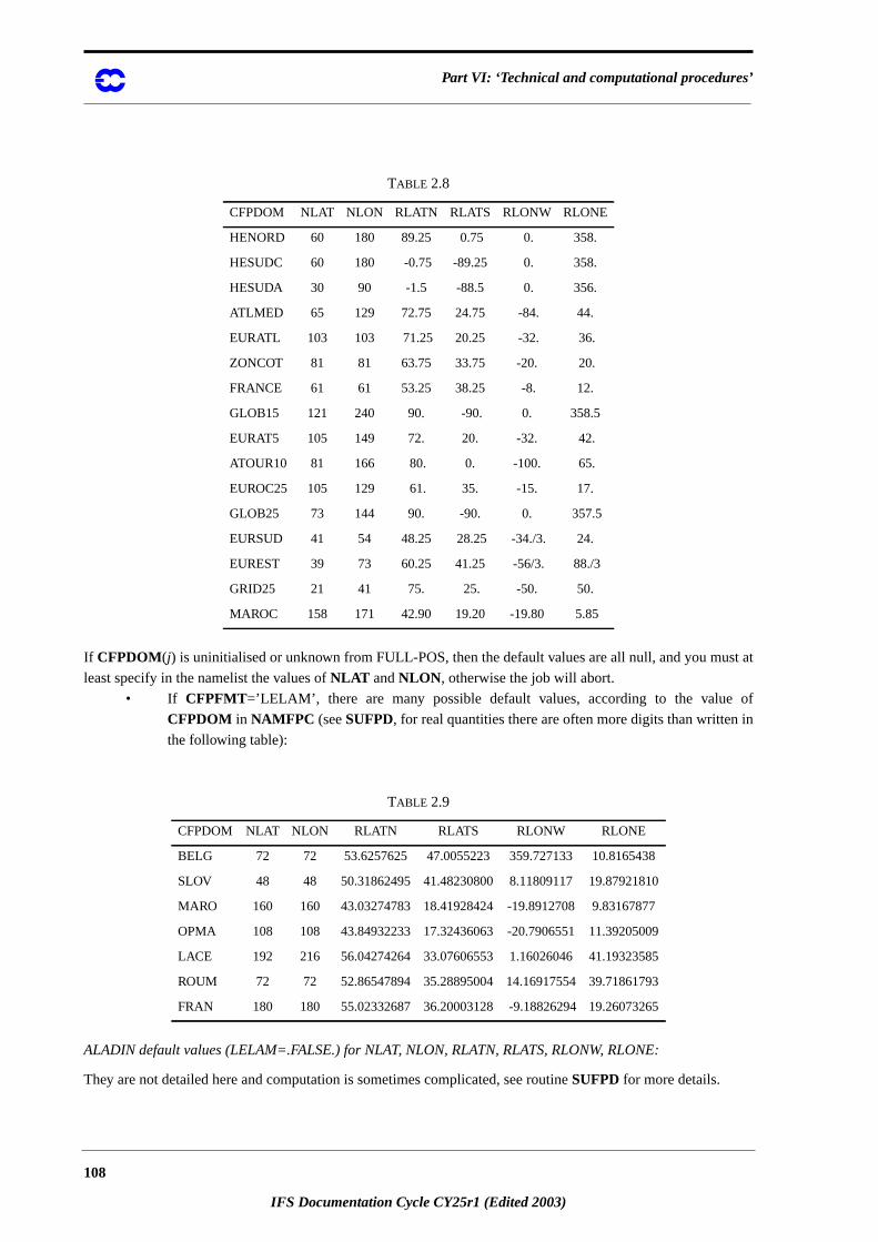
Part VI: ‘Technical and computational procedures’
st at
of
in
If CFPDOM(j) is uninitialised or unknown from FULL-POS, then the default values are all null, and you mu
least specify in the namelist the values ofNLAT andNLON , otherwise the job will abort.
• If CFPFMT=’LELAM’, there are many possible default values, according to the value
CFPDOM in NAMFPC (seeSUFPD, for real quantities there are often more digits than written
the following table):
ALADIN default values (LELAM=.FALSE.) for NLAT, NLON, RLATN, RLATS, RLONW, RLONE:
They are not detailed here and computation is sometimes complicated, see routineSUFPD for more details.
TABLE 2.8
CFPDOM NLAT NLON RLATN RLATS RLONW RLONE
HENORD 60 180 89.25 0.75 0. 358.
HESUDC 60 180 -0.75 -89.25 0. 358.
HESUDA 30 90 -1.5 -88.5 0. 356.
ATLMED 65 129 72.75 24.75 -84. 44.
EURATL 103 103 71.25 20.25 -32. 36.
ZONCOT 81 81 63.75 33.75 -20. 20.
FRANCE 61 61 53.25 38.25 -8. 12.
GLOB15 121 240 90. -90. 0. 358.5
EURAT5 105 149 72. 20. -32. 42.
ATOUR10 81 166 80. 0. -100. 65.
EUROC25 105 129 61. 35. -15. 17.
GLOB25 73 144 90. -90. 0. 357.5
EURSUD 41 54 48.25 28.25 -34./3. 24.
EUREST 39 73 60.25 41.25 -56/3. 88./3
GRID25 21 41 75. 25. -50. 50.
MAROC 158 171 42.90 19.20 -19.80 5.85
TABLE 2.9
CFPDOM NLAT NLON RLATN RLATS RLONW RLONE
BELG 72 72 53.6257625 47.0055223 359.727133 10.8165438
SLOV 48 48 50.31862495 41.48230800 8.11809117 19.87921810
MARO 160 160 43.03274783 18.41928424 -19.8912708 9.83167877
OPMA 108 108 43.84932233 17.32436063 -20.7906551 11.39205009
LACE 192 216 56.04274264 33.07606553 1.16026046 41.19323585
ROUM 72 72 52.86547894 35.28895004 14.16917554 39.71861793
FRAN 180 180 55.02332687 36.20003128 -9.18826294 19.26073265
108
IFS Documentation Cycle CY25r1 (Edited 2003)
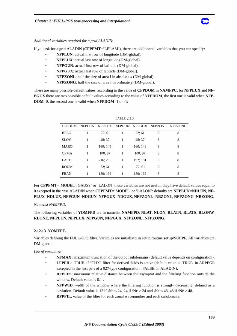
Chapter 2 ‘FULL-POS post-processing and interpolation’
l to
ion).
the
s a
Additional variables required for a grid ALADIN:
If you ask for a grid ALADIN (CFPFMT=’LELAM’), there are additionnal variables that you can specify:
• NFPLUN: actual first row of longitude (DM-global).
• NFPLUX : actual last row of longitude (DM-global).
• NFPGUN: actual first row of latitude (DM-global).
• NFPGUX: actual last row of latitude (DM-global).
• NFPZONL : half the size of area I in abscissax (DM-global).
• NFPZONG: half the size of area I in ordinatey (DM-global).
There are many possible default values, according to the value ofCFPDOM in NAMFPC ; for NFPLUX andNF-PGUX there are two possible default values according to the value ofNFPDOM, the first one is valid whenNFP-DOM=0, the second one is valid whenNFPDOM=1 or -1:
For CFPFMT=’MODEL’,’GAUSS’ or ’LALON’ these variables are not useful, they have default values equa
0 excepted in the case ALADIN whenCFPFMT=’MODEL’ or ’LALON’: defaults are NFPLUN=NDLUN , NF-PLUX=NDLUX , NFPGUN=NDGUN, NFPGUX=NDGUX, NFPZONL=NBZONL , NFPZONG=NBZONG.
Namelist NAMFPD:
The following variables ofYOMFPD are in namelistNAMFPD : NLAT , NLON , RLATN , RLATS , RLONW,
RLONE , NFPLUN, NFPLUX , NFPGUN, NFPGUX, NFPZONL , NFPZONG.
2.12.13 YOMFPF.
Variables defining the FULL-POS filter. Variables are initialised in setup routinesetup/SUFPF. All variables are
DM-global.
List of variables:
• NFMAX : maximum truncation of the output subdomains (default value depends on configurat
• LFPFIL : .TRUE. if “THX" filter for derived fields is active (default value is .TRUE. in ARPEGE
excepted in the first part of a 927-type configuration, .FALSE. in ALADIN).
• RFPEPS: maximum relative distance between the asymptot and the filtering function outside
window. Default value is 0.1 .
• NFPWID : width of the window where the filtering function is strongly decreasing; defined a
deviation. Default value is 12 if \Nc≤ 24, 24 if \Nc > 24 and \Nc≤ 48, 48 if \Nc > 48.
• RFPFIL : value of the filter for each zonal wavenumber and each subdomain.
TABLE 2.10
CFPDOM NFPLUN NFPLUX NFPGUN NFPGUX NFPZONL NFPZONG
BELG 1 72; 61 1 72; 61 8 8
SLOV 1 48; 37 1 48; 37 8 8
MARO 1 160; 149 1 160; 149 8 8
OPMA 1 108; 97 1 108; 97 8 8
LACE 1 216; 205 1 192; 181 8 8
ROUM 1 72; 61 1 72; 61 8 8
FRAN 1 180; 169 1 180; 169 8 8
109
IFS Documentation Cycle CY25r1 (Edited 2003)
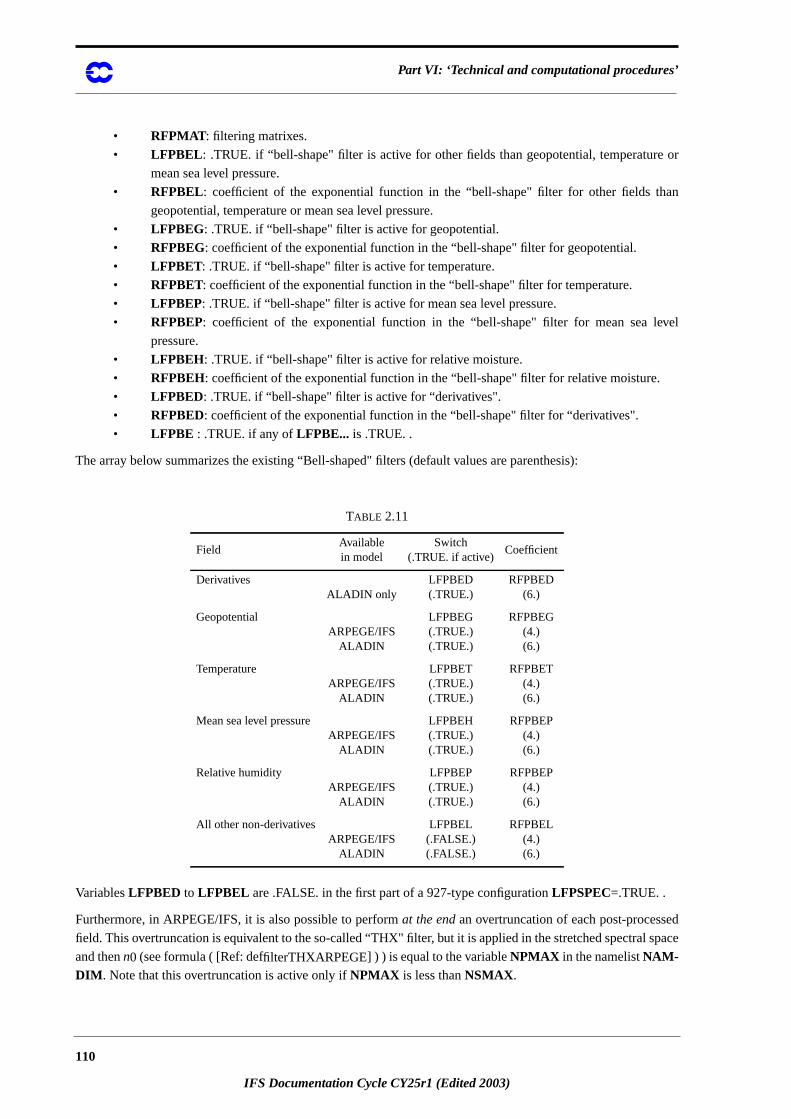
Part VI: ‘Technical and computational procedures’
or
an
vel
d
pace
• RFPMAT : filtering matrixes.
• LFPBEL : .TRUE. if “bell-shape" filter is active for other fields than geopotential, temperature
mean sea level pressure.
• RFPBEL: coefficient of the exponential function in the “bell-shape" filter for other fields th
geopotential, temperature or mean sea level pressure.
• LFPBEG: .TRUE. if “bell-shape" filter is active for geopotential.
• RFPBEG: coefficient of the exponential function in the “bell-shape" filter for geopotential.
• LFPBET: .TRUE. if “bell-shape" filter is active for temperature.
• RFPBET: coefficient of the exponential function in the “bell-shape" filter for temperature.
• LFPBEP: .TRUE. if “bell-shape" filter is active for mean sea level pressure.
• RFPBEP: coefficient of the exponential function in the “bell-shape" filter for mean sea le
pressure.
• LFPBEH : .TRUE. if “bell-shape" filter is active for relative moisture.
• RFPBEH: coefficient of the exponential function in the “bell-shape" filter for relative moisture.
• LFPBED: .TRUE. if “bell-shape" filter is active for “derivatives".
• RFPBED: coefficient of the exponential function in the “bell-shape" filter for “derivatives".
• LFPBE : .TRUE. if any ofLFPBE... is .TRUE. .
The array below summarizes the existing “Bell-shaped" filters (default values are parenthesis):
VariablesLFPBED to LFPBEL are .FALSE. in the first part of a 927-type configurationLFPSPEC=.TRUE. .
Furthermore, in ARPEGE/IFS, it is also possible to performat the endan overtruncation of each post-processe
field. This overtruncation is equivalent to the so-called “THX" filter, but it is applied in the stretched spectral s
and thenn0 (see formula ( [Ref: deffilterTHXARPEGE] ) ) is equal to the variableNPMAX in the namelistNAM-DIM . Note that this overtruncation is active only ifNPMAX is less thanNSMAX .
TABLE 2.11
FieldAvailablein model
Switch(.TRUE. if active)
Coefficient
DerivativesALADIN only
LFPBED(.TRUE.)
RFPBED(6.)
GeopotentialARPEGE/IFS
ALADIN
LFPBEG(.TRUE.)(.TRUE.)
RFPBEG(4.)(6.)
TemperatureARPEGE/IFS
ALADIN
LFPBET(.TRUE.)(.TRUE.)
RFPBET(4.)(6.)
Mean sea level pressureARPEGE/IFS
ALADIN
LFPBEH(.TRUE.)(.TRUE.)
RFPBEP(4.)(6.)
Relative humidityARPEGE/IFS
ALADIN
LFPBEP(.TRUE.)(.TRUE.)
RFPBEP(4.)(6.)
All other non-derivativesARPEGE/IFS
ALADIN
LFPBEL(.FALSE.)(.FALSE.)
RFPBEL(4.)(6.)
110
IFS Documentation Cycle CY25r1 (Edited 2003)
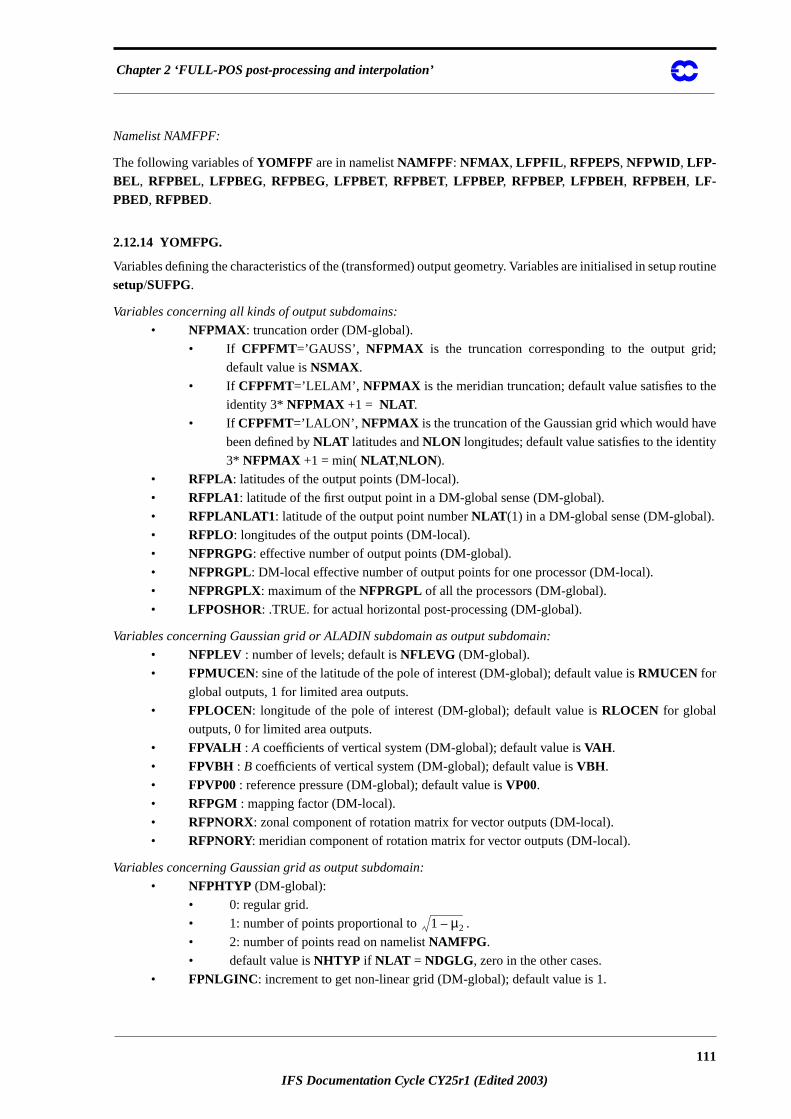
Chapter 2 ‘FULL-POS post-processing and interpolation’
routine
;
e
e
y
Namelist NAMFPF:
The following variables ofYOMFPF are in namelistNAMFPF : NFMAX , LFPFIL , RFPEPS, NFPWID , LFP-BEL , RFPBEL, LFPBEG, RFPBEG, LFPBET, RFPBET, LFPBEP, RFPBEP, LFPBEH , RFPBEH, LF-PBED, RFPBED.
2.12.14 YOMFPG.
Variables defining the characteristics of the (transformed) output geometry. Variables are initialised in setup
setup/SUFPG.
Variables concerning all kinds of output subdomains:
• NFPMAX : truncation order (DM-global).
• If CFPFMT=’GAUSS’, NFPMAX is the truncation corresponding to the output grid
default value isNSMAX .
• If CFPFMT=’LELAM’, NFPMAX is the meridian truncation; default value satisfies to th
identity 3* NFPMAX +1 = NLAT .
• If CFPFMT=’LALON’, NFPMAX is the truncation of the Gaussian grid which would hav
been defined byNLAT latitudes andNLON longitudes; default value satisfies to the identit
3* NFPMAX +1 = min(NLAT ,NLON ).
• RFPLA : latitudes of the output points (DM-local).
• RFPLA1: latitude of the first output point in a DM-global sense (DM-global).
• RFPLANLAT1 : latitude of the output point numberNLAT (1) in a DM-global sense (DM-global).
• RFPLO: longitudes of the output points (DM-local).
• NFPRGPG: effective number of output points (DM-global).
• NFPRGPL: DM-local effective number of output points for one processor (DM-local).
• NFPRGPLX: maximum of theNFPRGPL of all the processors (DM-global).
• LFPOSHOR: .TRUE. for actual horizontal post-processing (DM-global).
Variables concerning Gaussian grid or ALADIN subdomain as output subdomain:
• NFPLEV : number of levels; default isNFLEVG (DM-global).
• FPMUCEN: sine of the latitude of the pole of interest (DM-global); default value isRMUCEN for
global outputs, 1 for limited area outputs.
• FPLOCEN: longitude of the pole of interest (DM-global); default value isRLOCEN for global
outputs, 0 for limited area outputs.
• FPVALH : A coefficients of vertical system (DM-global); default value isVAH .
• FPVBH : B coefficients of vertical system (DM-global); default value isVBH .
• FPVP00: reference pressure (DM-global); default value isVP00.
• RFPGM : mapping factor (DM-local).
• RFPNORX: zonal component of rotation matrix for vector outputs (DM-local).
• RFPNORY: meridian component of rotation matrix for vector outputs (DM-local).
Variables concerning Gaussian grid as output subdomain:
• NFPHTYP (DM-global):
• 0: regular grid.
• 1: number of points proportional to .
• 2: number of points read on namelistNAMFPG .
• default value isNHTYP if NLAT = NDGLG , zero in the other cases.
• FPNLGINC : increment to get non-linear grid (DM-global); default value is 1.
1 µ2–
111
IFS Documentation Cycle CY25r1 (Edited 2003)
Part VI: ‘Technical and computational procedures’
eal
if
).
o in
3*
if
if
e
al);
ault
al);
• NFPRGRI : number of active points on a parallel (DM-global); default value isNLOENG if
NLAT = NDGLG , NLON in the other cases.
• NFPMEN : maximum zonal wave number for a given parallel (DM-global).
• FPSTRET : stretching factor (DM-global); default value isRSTRET for global outputs, 1 for
limited area outputs.
• NFPTTYP (DM-global):
• 1: no tilting; pole of high resolution at the northern pole of the real Earth.
• 2: tilting; pole of high resolution at a different location than the northern pole of the r
Earth.
Default value isNSTTYP for global outputs, 1 for limited area outputs.
• NFPQUAD : quadrature ( 1 : Gauss ; 2 : Lobatto); (DM-global); default value isNQUAD for
global outputs, 1 for limited area outputs.
• RFPMU : array containing the sines of the output Gaussian latitudes (DM-global).
• LFPOLE : .TRUE. if points at the poles are required; default value is .TRUE
CFPFMT=’MODEL’ or pseudo-configurations 927 and E927, .FALSE. elsewhere (DM-global
Variables concerning ALADIN grid as output subdomain:
• FPBETA: angle of rotation in degrees (DM-global); default value is zero in ARPEGE/IFS, zer
ALADIN if CFPFMT=’MODEL’ and EBETA in ALADIN in the other cases.
• NMFPMAX : meridian truncation order (DM-global); default value satisfies to the identity
NFPMAX +1 = NLAT if CFPFMT=’LELAM’ and default value is 1 in the other cases.
• LFPMAP : .T./.F. if the domain is defined through its coordinates/wavelengths (DM-global).
• FPLX : wavelength in longitude (DM-global); default is 5448300. in ARPEGE/IFS
CFPFMT=’LELAM’, 0 in ARPEGE/IFS if CFPFMT=’MODEL’, ’LALON’ or ’GAUSS’, 0 in
ALADIN if CFPFMT=’GAUSS’ and ELX in ALADIN if CFPFMT=’MODEL’, ’LALON’ or
’LELAM’.
• FPLY: wavelength in latitude (DM-global); default is 5448300. in ARPEGE/IFS
CFPFMT=’LELAM’, 0 in ARPEGE/IFS if CFPFMT=’MODEL’, ’LALON’ or ’GAUSS’, 0 in
ALADIN if CFPFMT=’GAUSS’ and ELY in ALADIN if CFPFMT=’MODEL’, ’LALON’ or
’LELAM’.
• NFPROTEQ: parameter for rotation (DM-global).
• 0: no rotation.
• 1: the reference point of rotation (FIR ,LAR ) is rotated to equator, the north pole is on th
new Greenwich meridian.
Default is 0 in ARPEGE/IFS, 0 in ALADIN ifCFPFMT=’GAUSS’ and NROTEQ in ALADIN if CFP-FMT =’MODEL’, ’LALON’ or ’LELAM’.
• FPLONR: LAR geographical longitude of reference point of rotation, in degrees (DM-glob
default value is zero in ARPEGE/IFS, 0 in ALADIN ifCFPFMT=’GAUSS’ and ELONR in
ALADIN if CFPFMT=’MODEL’, ’LALON’ or ’LELAM’.
• FPLATR : FIR geographical latitude of reference point of rotation, in degrees (DM-global); def
value is zero in ARPEGE/IFS, 0 in ALADIN ifCFPFMT=’GAUSS’ andELATR in ALADIN if
CFPFMT=’MODEL’, ’LALON’ or ’LELAM’.
• FPLON0: LA0 geographical longitude of reference for the projection, in degrees (DM-glob
default value is 0. in ARPEGE/IFS excepted in the caseCFPFMT=’LELAM’ (various default
values according toCFPDOM, see routineSUFPG1), 0. in ALADIN if CFPFMT=’GAUSS’ and
ELON0 in ALADIN if CFPFMT=’MODEL’, ’LALON’ or ’LELAM’.
112
IFS Documentation Cycle CY25r1 (Edited 2003)
Chapter 2 ‘FULL-POS post-processing and interpolation’
ault
FS
E/
E/
r than
xtracted
elds
ice
• FPLAT0 : FI0 geographical latitude of reference for the projection, in degrees (DM-global); def
value is 0. in ARPEGE/IFS excepted in the caseCFPFMT=’LELAM’ (various default values
according toCFPDOM, see routineSUFPG1), 0. in ALADIN if CFPFMT=’GAUSS’ and
ELAT0 in ALADIN if CFPFMT=’MODEL’, ’LALON’ or ’LELAM’.
• FPRPK: K projection parameter and definition (DM-global); default value is -9. in ARPEGE/I
excepted in the caseCFPFMT=’LELAM’ (various default values according toCFPDOM, see
routine SUFPG1), -9. in ALADIN if CFPFMT=’GAUSS’ and ERPK in ALADIN if
CFPFMT=’MODEL’, ’LALON’ or ’LELAM’.
• NFPSOTRP: isotropy parameter under projection (DM-global); default value is 0. in ARPEG
IFS excepted in the caseCFPFMT=’LELAM’ (generally 1.), 0. in ALADIN if
CFPFMT=’GAUSS’ andNSOTRP in ALADIN if CFPFMT=’MODEL’, ’LALON’ or ’LELAM’.
• NFPGIV0: choice of reference point for projection (DM-global); default value is zero in ARPEG
IFS, 0. in ALADIN if CFPFMT=’GAUSS’ and NGIV0 in ALADIN if CFPFMT=’MODEL’,
’LALON’ or ’LELAM’.
Variables concerning ALADIN or ’LALON’ grid as output subdomain:
• RFPDX: grid size in meters alongx if projection (ALADIN grid); longitude increment in radians if
spherical geometry (DM-global).
• RFPDY: grid size in meters alongy if projection (ALADIN grid); latitude increment in radians if
spherical geometry (DM-global).
Namelist NAMFPG:
The following variables ofYOMFPG are in namelistNAMFPG : NFPMAX , NFPLEV, FPMUCEN, FPLO-CEN, FPVALH , FPVBH, NFPHTYP, NFPRGRI, FPSTRET, NFPTTYP, NFPQUAD, FPBETA, LFPOLE ,
FPVP00, NMFPMAX , FPLX , FPLY, NFPROTEQ, FPLONR, FPLATR , FPLON0, FPLAT0 , FPRPK, NFP-SOTRP, NFPGIV0, FPNLGINC .
2.12.15 YOMFPIOS.
Contains control variables for FULL-POS IO scheme. Variables are initialised in setup routinesetup/SUFPIOS.
Writing to output files: variable NFPXFLD.
To write post-processed fields on an output file, you first extract them from an array (or a work file). Rathe
extracting the fields one after the other, the fields are grouped in packets, and these packets of fields are e
one after the other. You can specify the maximum number of fields in a packet by modifying the variableNFPX-FLD in the namelistNAMFPIOS . The default value is the maximum possible depending on the number of fi
to produce. Raising the value ofNFPXFLD should save CPU time to the detriment of the memory cost, and v
versa.
Variables for auxiliary fields:
• LIOFPR : switch for IO scheme (DM-global).
• CIOFPR : pathname (DM-global).
• NIOFPR : MIO package file reference (DM-global).
• NBLIOFPR : buffer length for IO (DM-local).
• NIOBFFPR: number of buffers for IO (DM-global).
• NPCKFFPR: packing factor (DM-global).
• NEXPBFPR: number of bits used for exponent when packing (DM-global).
Variables for working fields:
113
IFS Documentation Cycle CY25r1 (Edited 2003)
Part VI: ‘Technical and computational procedures’
els).
, no I/O
• LIOFPW : switch for IO scheme (DM-global).
• CIOFPW : pathname (DM-global).
• NIOFPW : MIO package file reference (DM-global).
• NBLIOFPW : buffer length for IO (DM-local).
• NIOBFFPW: number of buffers for IO (DM-global).
• NPCKFFPW: packing factor (DM-global).
• NEXPBFPW: number of bits used for exponent when packing (DM-global).
Variables for dynamics fields:
• LIOFPD : switch for IO scheme (DM-global).
• CIOFPD : pathname (DM-global).
• NIOFPD : MIO package file reference (DM-global).
• NBLIOFPD : buffer length for IO (DM-local).
• NIOBFFPD: number of buffers for IO (DM-global).
• NPCKFFPD: packing factor (DM-global).
• NEXPBFPD: number of bits used for exponent when packing (DM-global).
Variables for physics fields:
• LIOFPP : switch for IO scheme (DM-global).
• CIOFPP : pathname (DM-global).
• NIOFPP : MIO package file reference (DM-global).
• NBLIOFPP : buffer length for IO (DM-local).
• NIOBFFPP: number of buffers for IO (DM-global).
• NPCKFFPP: packing factor (DM-global).
• NEXPBFPP: number of bits used for exponent when packing (DM-global).
Variables for fields from APACHE:
• LIOFPA : switch for IO scheme (DM-global).
• CIOFPA : pathname (DM-global).
• NIOFPA : MIO package file reference (DM-global).
• NBLIOFPA : buffer length for IO (DM-local).
• NIOBFFPA : number of buffers for IO (DM-global).
• NPCKFFPA: packing factor (DM-global).
• NEXPBFPA: number of bits used for exponent when packing (DM-global).
Additional remarks and some default values:
For the horizontal post-processing, the data flows have been separated in 4 parts:
• post-processed dynamical data.
• post-processed physical and fluxes data.
• weights for horizontal interpolations.
• output geometry and climatology.
• horizontally pre-processed dynamical data (for post-processing on height levels or hybrid lev
To spare memory space, each of these data flows can be controlled by a specific I/O scheme. By default
scheme is activated. If you wish to activate I/O schemes, then use the variables which are in the namelistNAMF-PIOS as the array below describes it (defaults values are the ones in parenthesis).
114
IFS Documentation Cycle CY25r1 (Edited 2003)
Chapter 2 ‘FULL-POS post-processing and interpolation’
is
e
of
Namelist NAMFPIOS:
The following variables ofYOMFPIOS are in namelistNAMFPIOS : NFPXFLD , CIOFPR, CIOFPW,
CIOFPD, CIOFPP, CIOFPA , LIOFPR , NPCKFFPR, NEXPBFPR, LIOFPW , NPCKFFPW, NEXPBFPW,
LIOFPD , NPCKFFPD, NEXPBFPD, LIOFPP, NPCKFFPP, NEXPBFPP, LIOFPA , NPCKFFPA, NEX-PBFPA.
2.12.16 YOMFPOLE.
Useless, has to be removed.
2.12.17 YOMFPOP.
Contains post-processing file-handling variables. Variables are initialised in setup routinesetup/SUFPOPH. No
variable in namelist.
List of variables:
• CFPFN: path file name for output files (DM-global).
• CFPCA: names of output frames (DM-global).
2.12.18 YOMFPSC2.
Contains control variables forSCAN2MSM or SCAN2MDM FULL-POS rows. Variables are initialised in setup
routinesetup/SUFPSC2.
List of variables:
• NFPLENR: number of active points in each post-processing row (DM-local).
• NFPROMAG : working dimension for horizontal post-processing (DM-global if its value
specified in the namelistNAMFPSC2, DM-local in the contrary, default value depends on th
processor if distributed memory).
• NFPROMAL : working dimension for horizontal post-processing, DM-local version
NFPROMAG .
• NFPBSR: number of sub-rows in each post-processing row (DM-local).
• NFPTBSRL: total number of sub-rows in post-processing buffer (DM-local).
TABLE 2.12
Data .TRUE. to activate
I/O schemeWork file name Packing factor
Number of bits used forexponent when packing
Post-processeddynamical fields
LIOFPD(.FALSE.)
CIOFPD(’miofpdyn’)
NPCKFFPD(1)
NEXPBFPD(6)
Post-processedphys flds/fluxes
LIOFPP(.FALSE.)
CIOFPP(’miofpphy’)
NPCKFFPP(1)
NEXPBFPP(6)
Weights LIOFPW(.FALSE.)
CIOFPW(’miofpwork’)
NPCKFFPW(1)
NEXPBFPW(6)
Output geometry,climatology
LIOFPR(.FALSE.)
CIOFPR(’miofpaux’)
NPCKFFPR(1)
NEXPBFPR(6)
Pre-processeddynamical data
LIOFPA(.FALSE.)
CIOFPA(’miofpapa’)
NPCKFFPA(1)
NEXPBFPA(6)
115
IFS Documentation Cycle CY25r1 (Edited 2003)
Part VI: ‘Technical and computational procedures’
n the
some
e
ne a
ual
ections
y
r treats
e one
orted
ted to
ry) the
packet
y
cket.
o zero;
posite,
current
mes are
ser will
fol-
seful
tics: the
Additional remarks about variables NFPROMAG and NFPROMAL:
VariableNFPROMAG is very useful to find a compromise between the vectorization and the memory cost i
post-processing for the lagged computations (horizontal interpolations inHPOSLAG and additional calculations
in ENDVPOS), and it is also very useful to make efficient I/O schemes. The variableNFPROMAL represents the
horizontal depth of work in the lagged computations of post-processing; it is obvious that this variable has
similarity with the famous variableNPROMA (in namelistNAMDIM ) or the less famous variableNSEGM (in
namelistNAM926), but its use is more flexible. For shared memoryNFPROMAL =NFPROMAG if NFPRO-MAG is an odd integer,NFPROMAL =NFPROMAG+1 if NFPROMAG is an even integer; this is also the cas
if NFPROMAG is taken to its (DM-local) default value for distributed memory, this is not necessary to defi
unic DM-global value (but desirable in the future). For distributed memory when a DM-global value ofNFPRO-MAG is given in the namelistNAMFPSC2, NFPROMAL depends on the processor, its maximum value is eq
to NFPROMAG if NFPROMAG is an odd integer,NFPROMAG+1 if NFPROMAG is an even integer. Variable
NFPROMAG is used only inSUFPSC2, the remainder of the code uses onlyNFPROMAL . The way how the
post-processing data flow is managed in the post-processing arrays/work files is explained in detail in the s
’Some shared memory features’ and ’Some distributed memory features’. For summary:
• The model data is split in packets of points of fixed sizeNPROMA ; each model packet is treated b
one task, and is independent from the other packets. For distributed memory one processo
NGPTOT model grid-points, with a subdivision intoNPROMA -packets, but this subdivision is
active for not lagged computations only.
• Each output point (i.e. where post-processing is performed) is related to one model packet: th
which contains the model point which is the nearest from it. That way, the output points are s
out, so that each post-processing packet (i.e. the group of all the output points which are rela
the same model packet) has a specific size. For shared memory (resp. distributed memo
model-packets used to computeNFPROMAG andNFPROMAL are theNPROMA -packets (resp.
theNGPTOT-packets).
• In order to use the I/O subroutines already available in ARPEGE/IFS, each post-processing
has been split in sub-rows of fixed sizeNFPROMAL . Each post-processing packet is treated b
one task which performs a loop on the number of sub-rows in the current post-processing pa
• Note that an empty post-processing packet is characterized by a number of sub-rows equal t
as a consequence, empty post-processing packets do not lead to memory spill. On the op
each non-empty post-processing packet contains a specific number of unused words.
Searching for a compromise between vectorization and memory cost, the value ofNFPROMAG can be any integer
from 1 to the size of the biggest post-processing packet. The biggerNFPROMAG will be, the more the vectoriza-
tion will be efficient, and the more memory will be needed. The default value ofNFPROMAG is the mean size of
the post-processing packets if shared memory, the total number of post-processing points treated by the
processor if distributed memory, as this value appeared to be the best compromise. However, if the I/O sche
activated, the size of the biggest post-processing packet may be a more efficient value. In the listing, the u
find more information to find out the value to adopt: just before “COMMON YOMFPSC2" is printed out, the
lowing information is written (information depends on the processor for distributed memory but is not very u
in this case because there is only one value per processor which is used to compute the following statis
standard deviation is zero):
• size of the smallest post-processing packet.
• size of the biggest post-processing packet.
• mean size of the post-processing packets.
• standard deviation of the size of the post-processing packets.
116
IFS Documentation Cycle CY25r1 (Edited 2003)
Chapter 2 ‘FULL-POS post-processing and interpolation’
OST
e DM-
tput
puted
S.
parts:
cheme.
s
sed
You can also know the memory you have lost in the post-processing arrays: just locate “TOTAL MEMORY L
IN WORDS =" .
Namelist NAMFPSC2:
The following variable ofYOMFPSC2 is in namelistNAMFPSC2: NFPROMAG .
2.12.19 YOMFPSC2B.
Contains control variables forSCAN2MSM or SCAN2MDM FULL-POS sub-rows. Variables are initialised in
setup routinesetup/SUFPSC2B. No variable in namelist.
List of variables:
• NFPROF: number of active points in each post-processing sub-row (DM-local).
• NFPINT: number of points to be computed through 12-points interpolations (NFPINT (1,.)) and
through averaging of a box (NFPINT (2,.)). DM-local variable.
• NFPSORT: pointer of the interlaced post-processing points in the sorted array (DM-local).
• NFPSTAP: sub-row start pointer for each row (DM-local).
2.12.20 YOMFPSP.
Contains FULL-POS spectral arrays. Variables are initialised after direct spectral transforms. All variables ar
global. No variable in namelist.
List of variables:
• SPAFP: underived vertically post-processed fields.
• SPBFP: derived vertically post-processed fields for all required subdomains.
• SPDFP: derived vertically post-processed fields for one subdomain.
2.12.21 YOMFPT0.
Contains bufferFPTS0: Auxiliary surface grid point array for post-processing on height levels above an ou
orography and for surface horizontal post-processing above an output orography (DM-local). Variable is com
in routinepp_obs/GPOS. No variable in namelist.
2.12.22 YOMIOS.
Some variables inYOMIOS (which does not contain only FULL-POS variables) can be useful for FULL-PO
These variables are DM-global. For the vertical post-processing, the data flows have been separated in 2
• fitted post-processed fields.
• unfitted post-processed fields.
To spare memory space, the data flow of unfitted post-processed fields can be controlled by a specific I/O s
By default, this I/O scheme is activated only at ECMWF (LECMWF =.TRUE.). If you wish to activate/deactivate
it, just setLIOGAUX =.TRUE./.FALSE. in the namelistNAMCT0 . Then you can change other related variable
in the namelistNAMIOS :
• CIOGAUX : work file name of unfitted vertically post-processed fields; default is ’miogaux’.
• NPCKFGX : packing factor for I/O on vertically post-processed fields; default is 1.
• NEXPBGX: number of bits used for exponent when packing I/O on vertically post-proces
fields; default is 6.
Other useful variables in YOMIOS and NAMIOS:
117
IFS Documentation Cycle CY25r1 (Edited 2003)
Part VI: ‘Technical and computational procedures’
shared
ful
• CIOFOU1: work file name for Fourier data.
• NBLFOU : segment length for complex I/O on Fourier data.
• CIOLPOL : work file name for Legendre polynomials.
• CIOTMDT : work file name of grid-point fields at t-dt.
• NPCKFT9: packing factor for I/O on grid-point fields at t-dt.
• NEXPBT9: number of bits for exp. when packing grid-point fields at t-dt.
• CIOGPUA : work file name of upper air grid-point fields.
• NPCKFGU: packing factor for I/O on upper air grid-point fields.
• NEXPBGU: number of bits for exp. when packing upper air grid-point fields.
• CIOGPP : work file name of surface fields.
• NPCKFGP: packing factor for I/O on surface fields.
• NEXPBGP: number of bits for exp. when packing surface fields.
• CIOCFU : work file name of cumulated fluxes.
• NPCKFCF: packing factor for I/O on cumulated fluxes.
• NEXPBCF: number of bits for exp. when packing cumulated fluxes.
• CIOXFU : work file name of instantaneous fluxes.
• NPCKFXF : packing factor for I/O on instantaneous fluxes.
• NEXPBXF: number of bits for exp. when packing instantaneous fluxes.
• CIOSPEC: work file name of saved spectral data.
• CIOSUA : work file name of saved upper air grid-point data.
• CIOSSU : work file name of saved surface data.
• CIOSCF : work file name of saved cumulated fluxes data.
• CIOSXF : work file name of saved instantaneous fluxes data.
Default value of a variable of the typeCIONAME (for ex. CIOGPP) is ’mioname’ (for ex. ’miogpp’). Default
value ofNBLFOU depends on configuration. Default value ofNPCK... variables is 1. Default value ofNEXP...variables is 6. See routineSUIOS for more details.
2.12.23 YOMMP.
Variables specific to the distributed memory environment. Some of these variables can be used also for
memory. The following variables ofYOMMP (which does not contain only FULL-POS variables) can be use
for FULL-POS. Variables are generally computed insetup/SUMP0 (called bysetup/SU0Y0MA), setup/SUMP,
sometimessetup/SUCT0.
Variables describing distributed memory parallelization:
• MYPOS(1): own position in x-direction (DM-global).
• MYPOS(2): own position in y-direction (DM-global).
• MYPROC : own processor, quasi 1D position in torus (DM-local).
• MYSETA : own processor set A (set A DM-local, set B DM-global).
• MYSETB : own processor set B (set A DM-global, set B DM-local).
• MYPID : own process identifier (DM-local).
• MYFATHER : father process (DM-local).
• NSONS: number of son processes (DM-local).
• NPHASE: number of phases in the recursive transposition (DM-global). Default value is 1.
• NLAGA : lagging factor for tranpositions in A-direction (DM-global). Default value is 0.
• NLAGB : lagging factor for tranpositions in B-direction (DM-global). Default value is 0.
118
IFS Documentation Cycle CY25r1 (Edited 2003)
Chapter 2 ‘FULL-POS post-processing and interpolation’
tion
-
-
lue
ault
0.
is
SE.
fault
s in
int
ation
l).
l).
• NSLPAD: number of pad words initialised to a huge number at either of side of the interpola
buffer halo, used to trap halo problem (DM-global). Default value is 0.
• LSPLITIN : input data provided in sequential files if .TRUE. or in directories if .FALSE. (DM
global). Default value is .FALSE. .
• LSPLITOUT : output data provided in sequential files if .TRUE. or in directories if .FALSE. (DM
global). Default value is .TRUE. .
• NSTRIN: number of processors required to perform input processing (DM-global). Default va
is 1.
• NSTROUT: number of processors required to perform output processing (DM-global). Def
value is 0.
• NFLDIN : number of input fields to be buffered during distribution (DM-global). Default value is
• NFLDOUT : number of output fields to be buffered during gathering (DM-global). Default value
0.
• NPRCIDS: array containing the process identificators (DM-local).
• LAPPLE : defines apple or orange grid point decomposition (DM-global). Default value is .FAL
.
• LSPLIT : .TRUE./.FALSE.: latitudes are shared/not shared between sets (DM-global). De
value is .TRUE. for configurations between 100 and 199, .FALSE. for other configurations.
• LSLSYNC: .TRUE. if communication between processors for interpolation buffers reads/write
synchronisation (DM-global). Default value is .TRUE. .
Variables describing the partitioning of data:
• NDWIDE : width of interpolation buffer halo region (DM-global). Default value is 32.
• NPROCM: gives process which is responsible for the zonal wave numberm (DM-global).
• NUMPROCGP: gives processor which is responsible for model grid point (DM-global).
• NUMPROCFP: gives processor which is responsible for FULL-POS horizontal interpolation po
jfp, wherejfp = 1 toNFPRGPG (DM-global).
• NUMPP: tells for how many wave numbers the processes are responsible for the trunc
NSMAX (DM-local).
• NALLMS : global wave numbers for all processes (DM-global).
• NPTRMS: pointer to first wave number of given process inNALLMS (DM-global).
• NLATLS : first latitude for which current process calculates Legendre polynomials (DM-globa
• NLATLE : last latitude for which current process calculates Legendre polynomials (DM-globa
• NPROCL: gives process which is responsible for latitude in grid-point space (DM-global).
• NPROCLF: gives process which is responsible for latitude in Fourier space (DM-global).
• NULTPP: number of latitudes in given process in grid-point space (DM-global).
• NULTPPF: number of latitudes in given process in Fourier space (DM-global).
• MYLATS : latitude numbers mapped to current process in grid-point space (DM-global).
• NPTRLS: pointer to first global latitude of given process in grid-point space (DM-global).
• NPTRLSF: pointer to first global latitude of given process in Fourier space (DM-global).
• NFRSTLAT : first latitude of each set in grid-point space (DM-global).
• NFRSTLATF : first latitude of each set in Fourier space (DM-global).
• NFRSTLOFF: offset for first lat of own set in grid-point space (DM-local).
• NFRSTLOFFF: offset for first lat of own set in Fourier space (DM-local).
• NLSTLAT : last latitude of each set in grid-point space (DM-global).
• NLSTLATF : last latitude of each set in Fourier space (DM-global).
• NPTRFRSTLAT : pointer to first latitude in grid-point space (DM-global).
119
IFS Documentation Cycle CY25r1 (Edited 2003)
Part VI: ‘Technical and computational procedures’
e) A-
rsive)
e) B-
rsive)
rsive)
the
rsive)
the
obal
obal
al).
his
cal).
set B
).
• NPTRFRSTLATF : pointer to first latitude in Fourier space (DM-global).
• NPTRLSTLAT : pointer to last latitude in grid-point space (DM-global).
• NPTRLSTLATF : pointer to last latitude in Fourier space (DM-global).
• NPTRFLOFF : offset for pointer to first latitude of own set in grid-point space (DM-local).
• NPTRFLOFFF : offset for pointer to first latitude of own set in Fourier space (DM-local).
• NPTRLAT : pointer to start of latitude in grid-point space (DM-global).
• NPTRLATF : pointer to start of latitude in Fourier space (DM-global).
• LSPLITLAT : .TRUE. if latitude is split over two A sets (DM-global).
• MYFRSTACTLAT : first actual latitude of each processor in grid-point space (DM-global).
• MYLSTACTLAT : last actual latitude of each processor in grid-point space (DM-global).
• MYSENDA : processors to which current processor will send messages during the (recursiv
transposition (set A DM-local, set B DM-global).
• MYRECVA : processors from which current processor will receive messages during the (recu
A-transposition (set A DM-local, set B DM-global).
• MYSENDB: processors to which current processor will send messages during the (recursiv
transposition (DM-local).
• MYRECVB : processors from which current processor will receive messages during the (recu
B-transposition (DM-local).
• MYSENDSETA: process-set to which current processor will send messages during the (recu
A-transposition (set A DM-local, set B DM-global).
• MYRECVSETA : process-set to which current processor will receive messages during
(recursive) A-transposition (set A DM-local, set B DM-global).
• MYSENDSETB: process-set to which current processor will send messages during the (recu
B-transposition (set A DM-global, set B DM-local).
• MYRECVSETB : process-set to which current processor will receive messages during
(recursive) B-transposition (set A DM-global, set B DM-local).
• MYSENDG: processors to which current processor will send messages during gl
communication (DM-local).
• MYRECVG : processors from which current processor will receive messages during gl
communication (DM-local).
• MYMSGS: identification of the origin of the messages during recursive transposition (DM-loc
• NPTRSV: pointer to first spectral wave column on given process forNSMAX arrays (DM-global).
• NPTRSVV: asNPTRSV but for full m-columns (DM-global).
• NPTRMF : distribution of m-columns among B sets used for semi-implicit calculations on t
processor (fullm-columns case, set A DM-global, set B DM-local).
• NSPSTAF: pointer to where eachm-column starts; used for semi-implicit (fullm-columns case, set
A DM-global, set B DM-local).
• NUMLL : distribution of levels on B-processor set (DM-global).
• NPTRLL : pointer to first level on this B-processor set (set A DM-global, set B DM-local).
• NPSP: equals 1 if pressure is handled by this B-processor set (set A DM-global, set B DM-lo
• NPSURF: equals 1 if surface pressure is handled by this B-processor set (set A DM-global,
DM-local).
• NBSETLEV: on which B-set do the level belongs (set A DM-global, set B DM-local).
• NBSETSP: min(NFLEVG +1,NPROCB) (set A DM-global, set B DM-local).
• MYLEVS : level numbers mapped to current process (set A DM-global, set B DM-local).
• NVMODIST : normal modes mapped to the different B-sets (set A DM-global, set B DM-local
• NSPEC2V: number of spectral columns computed by this process forNSMAX arrays (DM-local).
120
IFS Documentation Cycle CY25r1 (Edited 2003)
Chapter 2 ‘FULL-POS post-processing and interpolation’
are
t in
-
t B
-
M-
l).
al).
-
-
(in
d from
in
• NSPEC2VF: number of spectral columns computed by this process if complete columns
required (DM-local).
• NSTA: start position of grid columns on latitudes (set A DM-global, set B DM-local).
• NONL : number of grid columns on latitudes (set A DM-global, set B DM-local).
• NGPSET: number of grid points of this processor in grid point space which also belong to i
Fourier space (set A DM-global, set B DM-local).
• NAPLAT : number of apple latitudes at the poles (DM-global). Default value is 0.
• NGPTRSEND: defines grid columns to be sent to each B-set duringTRGTOL (DM-local).
• NGPTRRECV: defines B-sets to receive from grid columns duringTRGTOL (DM-local).
SUFPCSET and SUFPRSET variables (based on NFPWIDE) used for FULL-POS interpolations:
• NAFPB1: local inner dimension of interpolation buffer used for FULL-POS interpolations (DM
local).
• NFPSTA: interpolation buffer start position of grid columns on latitudes (set A DM-global, se
DM-local).
• NFPONL: interpolation buffer number of grid column on latitudes (set A DM-global, set B DM
local).
• NFPOFF: interpolation buffer offset to start of each row inFPBUF1 andFPBUF2 (set A DM-
global, set B DM-local).
• NFPEXT: interpolation buffer extend latitudes over poles support (set A DM-global, set B D
local).
• NFPSTLAT: latitudinal position in the interpolation buffer during the data sending (DM-local).
• NFPSTLON: longitudinal position in the interpolation buffer during the data sending (DM-loca
• NFPRSTLAT: latitudinal position in the interpolation buffer during the data reception (DM-loc
• NFPRSTLON: longitudinal position in the interpolation buffer during the data reception (DM
local).
• NFPSENDNUM: length of the sent interpolation buffer (DM-local).
• NFPRECVNUM : length of the received interpolation buffer (DM-local).
• NFPCORE: offsets to core region points in interpolation buffer (set A DM-global, set B DM
local).
Some other variables:
• NCOMBFLEN : size of communication buffer. This is the maximum per processor buffer space
words) that the ARPEGE/IFS should use for one or more sends before receives are issue
destination processors (DM-global). Default value is 1800000.
• LBIDIR : .TRUE. if bi-directional transpositions are preferred (DM-global). Only implemented
the A-direction and require even number of processors. Default value is .FALSE. .
• LSNDS: logical indicating whether to send (resp. receive) data to southern set inTRLTOG (resp.
TRGTOL ) (DM-local).
• LSNDN: logical indicating whether to send (resp. receive) data to northern set inTRLTOG (resp.
TRGTOL ) (DM-local).
• LRCVS: logical indicating whether to receive (resp. send) data from southern set inTRLTOG(resp.TRGTOL ) (DM-local).
• LRCVN : logical indicating whether to receive (resp. send) data from northern set inTRLTOG(resp.TRGTOL ) (DM-local).
• NSNDS: number of messages to send (resp. receive) to southern set inTRLTOG (resp.TRGTOL )
(DM-local).
121
IFS Documentation Cycle CY25r1 (Edited 2003)
Part VI: ‘Technical and computational procedures’
d for
al).
g and
M-
lised
• NSNDN: number of messages to send (resp. receive) to northern set inTRLTOG (resp.TRGTOL )
(DM-local).
• Other distributed memory environment variables which are currently in another place, an
which YOMMP would be a better place:
• NUMP (in YOMDIM ): number of spectral waves handled by this processor (DM-loc
NUMP=NSMAX+1 for shared memory.
• NUMCP (in YOMDIM ): same as NUMP, but related to NCMAX (DM-local).
NUMCP=NCMAX +1 for shared memory.
• NUMTP (in YOMDIM ): same as NUMP, but related to NTMAX (DM-local).
NUMTP=NTMAX +1 for shared memory.
• MYMS (in YOMLAP ): actual wave numbers handled by each processor (DM-global).
Namelist NAMPAR1:
Initialize variables that control layout of distribution. The following variables ofYOMMP are in namelist
NAMPAR1 , namelist reading and default values calculations are done inSUMP0: LSPLIT , LSLSYNC, LAP-PLE, LBIDIR , NSLPAD, NAPLAT , NPHASE, NLAGA , NLAGB , NSTRIN, NSTROUT, NFLDIN , NFLD-OUT, NVALAG , NCOSTLAG , NLAGBDY , LSPLITIN , LSPLITOUT , NCOMBFLEN
2.12.24 YOMMPG.
Variables specific to the distributed memory environment. DM-global variables mainly used to handle readin
writing of grib data. Some of these variables can be used also for shared memory. Some variables inYOMMPG(which does not contain only FULL-POS variables) can be useful for FULL-POS. No variable in namelist.
• NPOSSP: defines partitioning of global spectral fields among processors (DM-global).
• NPOSCP: asNPOSSP for NCMAX arrays (DM-global).
• NPOSTP: asNPOSSP for NTMAX arrays (DM-global).
• NDIM0G : defines partitioning of global spectral fields among processors (DM-global).
2.12.25 YOMOP.
Some variables inYOMOP (which does not contain only FULL-POS variables) and namelistNAMOPH can be
useful for FULL-POS.
• LINC : .T. to get time stamp in hours rather than in time steps (default value is .FALSE.). D
global variable.
2.12.26 YOMPFPB.
Contains buffer for fully post-processed physical fields. Variables are initialised in setup routinesetup/SUFPSC2B. No variable in namelist.
List of variables:
• NLENPFPBL : length of buffer (DM-local).
• GPFPBUF : buffer (DM-local).
• NSTAPFPB : start adresses for post-processed packets of points within buffer (DM-local).
2.12.27 YOMRFPB.
Contains buffer of auxiliary fields (geometry, climatology) for horizontal post-processing. Variables are initia
in setup routinessetup/SURFPBUF for bufferRFPBUF andsetup/SUFPSC2Bfor other variables. No variable
122
IFS Documentation Cycle CY25r1 (Edited 2003)
Chapter 2 ‘FULL-POS post-processing and interpolation’
in FULL-
in namelist.
List of variables:
• NLENRFPBL : length of buffer (DM-local).
• RFPBUF : buffer containing output climatology and geometry (DM-local).
• NSTARFPB : start adresses for post-processed packets of points within buffer (DM-local).
2.12.28 YOMRFPDS.
Description of auxiliary fields for horizontal post-processing. Variables are initialised in setup routinesetup/SUR-FPDS. Variables are DM-global. No variable in namelist.
Field pointers:
• MFPGMO : for output mapping factor.
• MFPGNXO : for outputx-component of rotation matrix.
• MFPGNYO : for outputy-component of rotation matrix.
• MFPLSMO : for output land-sea mask.
• MFPFISO: for output surface geopotential.
• MFPFISI : for interpolated input surface geopotential.
• MFPCSTO: for output climatological surface temperature.
• MFPCSWO: for output climatological relative surface moisture.
• MFPSDO : for output climatological snow cover.
• MFPRSTO: for output relaxation deep soil temperature.
• MFPRSWO: for output relaxation deep soil moisture.
• MFPDSTO: for output climatological deep soil temperature.
• MFPDSWO: for output climatological relative deep soil moisture.
• MFPALBO : for output albedo.
• MFPEMIO : for output emissivity.
• MFPDEVO : for output (standard deviation) .
• MFPVEGO : for output vegetation.
• MFPGZ0O: for output .
• MFPANIO : for output anisotropy.
• MFPDIRO : for output direction.
Other variables:
• NFPVSO: number of climatological fields.
• CFPVSO: ARPEGE field names of the climatological fields.
• NRFPOS: total number of fields inRFPBUF.
2.12.29 YOMSC2.
Contains parameters used to control vectorisation and memory space. Some of these parameters are used
POS. No variable in namelist.
• NSLBCT: packet control array forSCAN2MSM or SCAN2MDM (DM-local). Packets are
NPROMA -packets for shared memory,NGPTOT-packets for distributed memory.
• NSLBCT(1,.): start row of packet.
• NSLBCT(2,.): end row of packet.
• NSLBCT(3,.): 1 if non-lagged grid-point computations on packet, 0 if not.
• NSLBCT(4,.): 1 if lagged grid-point computations on packet, 0 if not.
g×
z0 g×
123
IFS Documentation Cycle CY25r1 (Edited 2003)
Part VI: ‘Technical and computational procedures’
n
ry
ged
ged
• NSLBCT(5,.): usage ofSLBUF1 for packet (semi-Lagrangian scheme).
• NSLBCT(6,.): usage ofSLBUF2 for packet (semi-Lagrangian and Eulerian schemes).
• NSLBCT(7,.): usage ofFPBUF1 for packet (FULL-POS interpolations for fields other tha
surface physics).
• NSLBCT(8,.): usage ofFPBUF2 for packet (FULL-POS interpolations for surface
physics).
• NSLBCT(5,.) toNSLBCT(8,.) are useless for distributed memory. For distributed memo
NSLBCT(1,1)=NSLBCT(2,1)=NSLBCT(3,1)=NSLBCT(4,1)=1, the other values are
useless.
• NSLBR: number of packets of rows (DM-local). Packets areNPROMA -packets for shared
memory,NGPTOT-packets for distributed memory.NSLBR=1 for distributed memory.
• NLOCKFP1 : multitasking lock for interpolation bufferFPBUF1 used in FULL-POS. Useless for
distributed memory.
• NLOCKFP2 : multitasking lock for interpolation bufferFPBUF2 used in FULL-POS. Useless for
distributed memory.
• NLOCKOBL : multitasking lock for COBSLAGAD and COBSLAG. Useless for distributed
memory.
• NFPB1EV: event for interpolation bufferFPBUF1 used in FULL-POS. Useless for distributed
memory.
• NFPB2EV: event for interpolation bufferFPBUF2 used in FULL-POS. Useless for distributed
memory.
• NWEVFP1: number of tasks waiting for interpolation bufferFPBUF1 event used in FULL-POS.
Useless for distributed memory.
• NWEVFP2: number of tasks waiting for interpolation bufferFPBUF2 event used in FULL-POS.
Useless for distributed memory.
• NSLWIDE : number of rows the model lagged part runs behind (DM-global).
• NFPWIDE : number of rows the FULL-POS lagged part runs behind (DM-global).
• NFPB1:
• for shared memory: number of buffers (last dimension) for interpolation bufferFPBUF1used in FULL-POS.
• for distributed memory: used to dimension an interpolation buffer but only in the non lag
part of calculations;NFPB1=NGPBLKS (DM-local).
• NFPB2:
• for shared memory: number of buffers (last dimension) for interpolation bufferFPBUF2used in FULL-POS.
• for distributed memory: used to dimension an interpolation buffer but only in the non lag
part of calculations;NFPB2=NGPBLKS (DM-local).
• NSTABUF: start address for each row in grid-point buffers (DM-local).
• NLATPBF : packet pointer for each row in interpolation buffers (DM-local).
• NDIST: start address for each row in grid-point calculations (DM-local).
• NDIEND : end address for each row in grid-point calculations (DM-local).
• NCIST: start address for each row of grid-point field in buffer (DM-local).
• NCIEND : end address for each row of grid-point field in buffer (DM-local).
• NBFPFP1 (resp.NBFPFP2):• elements (1,.): pointer to packet contained in each buffer (FPBUF1, resp. FPBUF2).
• elements (2,.): remaining users of buffer (FPBUF1, resp. FPBUF2).
124
IFS Documentation Cycle CY25r1 (Edited 2003)
Chapter 2 ‘FULL-POS post-processing and interpolation’
for
setup
w
DM-global variables.
• NSC2EVH: event for each row indicating non-lagged part complete for FULL-POS. Useless
distributed memory.
2.12.30 YOMVFP.
Contains switches to use FULL-POS in an incremental variational application. Variables are initialised in
routinevar/SUVAR (move to directorysetup will be desirable in the future). Variables are DM-global.
List of variables:
• LARCHFP : .T. => FULL-POS will be used for communication between the high and lo
resolution run. Default is .F.
• LREFFP : .T. => the reference field is post-processed at high resolution. Default is .F.
• LRFTLFP : .T. => the reference field is post-processed at low resolution. Default is .F.
• LANAFP : .T. => the final (analysis) field is post-processed. Default is .F.
Namelist NAMVFP:
The following variable ofYOMVFP is in namelistNAMVFP : LARCHFP.
2.12.31 YOMVPOS.
Contains control variables for vertical post-processing. Variables are initialised in setup routinesetup/SUVFPOSand can be modified by routinetransform /UPDVPOS. All variables are DM-global. No variable in namelist.
Control variables for post-processing of 3D variables.
• LFIT3 : .T./.F. if 3D post-processed fields are fitted/not fitted.
• Scalar variablesNADD...: address in arrayGT1.
• NADDWIND : address of wind.
• NADDPSI : address of potential velocity.
• NADDDIV : address of divergence.
• NADDVOR : address of relative vorticity.
• NADDABS : address of absolute vorticity.
• NXFPLEV : number of post-processing levels.
• XFPLEV : values of post-processing levels. Array dimensioned toNXFPLEV .
• Scalar variablesNLEV...: number of post-processing (pp) levels for different variables.
• NLEVGEOP : number of pp levels for geopotential.
• NLEVTEMP : number of pp levels for temperature.
• NLEVUMOM : number of pp levels forU-wind component.
• NLEVVMOM : number of pp levels forV-wind component.
• NLEVSHUM : number of pp levels for specific humidity.
• NLEVRHUM : number of pp levels for relative humidity.
• NLEVVVEL : number of pp levels for vertical velocity.
• NLEVLWAT : number of pp levels for liquid water.
• NLEVSNOW : number of pp levels for solid water.
• NLEVCLFR : number of pp levels for cloud fraction.
• NLEVSCVA : number of pp levels for passive scalars.
• NLEVDIVE : number of pp levels for divergence.
• NLEVVORT : number of pp levels for relative vorticity.
• NLEVPSI : number of pp levels for velocity potential.
125
IFS Documentation Cycle CY25r1 (Edited 2003)
Part VI: ‘Technical and computational procedures’
t
• NLEVKHI : number of pp levels for stream function.
• NLEVTETA : number of pp levels for potential temperature.
• NLEVTHPW : number of pp levels for .
• NLEVWIND : number of pp levels for wind velocity.
• NLEVEPTH : number of pp levels for equivalent potential temperature.
• NLEVABSV : number of pp levels for absolute vorticity.
• NLEVSTDF : number of pp levels for stretching deformation.
• NLEVSHDF : number of pp levels for shearing deformation.
• NLEVPOTV : number of pp levels for potential vorticity.
• NLEVWEPV : number of pp levels for wet potential vorticity.
• NLEVPRES : number of pp levels for pressure.
• NLEVUA01 to NLEVUA16 : number of pp levels for upper air fields nr 01 to 16.
• ArraysNLVP... (dimensioned withNFPXLEV ): level pointers for different variables.
• NLVPGEOP : level pointers for geopotential.
• NLVPTEMP : level pointers for temperature.
• NLVPUMOM : level pointers forU-wind component.
• NLVPVMOM : level pointers forV-wind component.
• NLVPSHUM : level pointers for specific humidity.
• NLVPRHUM : level pointers for relative humidity.
• NLVPVVEL : level pointers for vertical velocity.
• NLVPLWAT : level pointers for liquid water.
• NLVPSNOW : level pointers for solid water.
• NLVPCLFR : level pointers for cloud fraction.
• NLVPSCVA : level pointers for passive scalars.
• NLVPDIVE : level pointers for divergence.
• NLVPVORT : level pointers for relative vorticity.
• NLVPPSI : level pointers for velocity potential.
• NLVPKHI : level pointers for stream function.
• NLVPTETA : level pointers for potential temperature.
• NLVPTHPW : level pointers for .
• NLVPWIND : level pointers for wind velocity.
• NLVPEPTH : level pointers for equivalent potential temperature.
• NLVPABSV : level pointers for absolute vorticity.
• NLVPSTDF : level pointers for stretching deformation.
• NLVPSHDF : level pointers for shearing deformation.
• NLVPPOTV : level pointers for potential vorticity.
• NLVPWEPV : level pointers for wet potential vorticity.
• NLVPPRES : level pointers for pressure.
• NLVPUA01 to NLVPUA16 : level pointers for upper air fields nr 01 to 16.
• ArraysNSDO...(dimensioned withNFPXLEV ): number of subdomains for each level of differen
variables.
• NSDOGEOP: number of subdomains for each level of geopotential.
• NSDOTEMP : number of subdomains for each level of temperature.
• NSDOUMOM : number of subdomains for each level ofU-wind component.
• NSDOVMOM : number of subdomains for each level ofV-wind component.
• NSDOSHUM : number of subdomains for each level of specific humidity.
• NSDORHUM : number of subdomains for each level of relative humidity.
θ′w
θ′w
126
IFS Documentation Cycle CY25r1 (Edited 2003)
Chapter 2 ‘FULL-POS post-processing and interpolation’
.
01
• NSDOVVEL : number of subdomains for each level of vertical velocity.
• NSDOLWAT : number of subdomains for each level of liquid water.
• NSDOSNOW : number of subdomains for each level of solid water.
• NSDOCLFR : number of subdomains for each level of cloud fraction.
• NSDOSCVA : number of subdomains for each level of passive scalars.
• NSDODIVE : number of subdomains for each level of divergence.
• NSDOVORT : number of subdomains for each level of relative vorticity.
• NSDOPSI: number of subdomains for each level of velocity potential.
• NSDOKHI : number of subdomains for each level of stream function.
• NSDOTETA : number of subdomains for each level of potential temperature.
• NSDOTHPW : number of subdomains for each level of .
• NSDOWIND : number of subdomains for each level of wind velocity.
• NSDOEPTH : number of subdomains for each level of equivalent potential temperature
• NSDOABSV : number of subdomains for each level of absolute vorticity.
• NSDOSTDF : number of subdomains for each level of stretching deformation.
• NSDOSHDF : number of subdomains for each level of shearing deformation.
• NSDOPOTV : number of subdomains for each level of potential vorticity.
• NSDOWEPV : number of subdomains for each level of wet potential vorticity.
• NSDOPRES: number of subdomains for each level of pressure.
• NSDOUA01 to NSDOUA16: number of subdomains for each level of upper air fields nr
to 16.
• Arrays NSDP... (dimensioned with(NFPDOM,NFPXLEV) ): subdomains pointers for different
variables.
• NSDPGEOP: subdomains pointers for geopotential.
• NSDPTEMP : subdomains pointers for temperature.
• NSDPUMOM : subdomains pointers for U-wind component.
• NSDPVMOM : subdomains pointers for V-wind component.
• NSDPSHUM : subdomains pointers for specific humidity.
• NSDPRHUM : subdomains pointers for relative humidity.
• NSDPVVEL : subdomains pointers for vertical velocity.
• NSDPLWAT : subdomains pointers for liquid water.
• NSDPSNOW: subdomains pointers for solid water.
• NSDPCLFR : subdomains pointers for cloud fraction.
• NSDPSCVA: subdomains pointers for passive scalars.
• NSDPDIVE : subdomains pointers for divergence.
• NSDPVORT : subdomains pointers for relative vorticity.
• NSDPPSI: subdomains pointers for velocity potential.
• NSDPKHI : subdomains pointers for stream function.
• NSDPTETA : subdomains pointers for potential temperature.
• NSDPTHPW : subdomains pointers for .
• NSDPWIND : subdomains pointers for wind velocity.
• NSDPEPTH : subdomains pointers for equivalent potential temperature.
• NSDPABSV: subdomains pointers for absolute vorticity.
• NSDPSTDF: subdomains pointers for stretching deformation.
• NSDPSHDF: subdomains pointers for shearing deformation.
• NSDPPOTV : subdomains pointers for potential vorticity.
• NSDPWEPV : subdomains pointers for wet potential vorticity.
θ′w
θ′w
127
IFS Documentation Cycle CY25r1 (Edited 2003)
Part VI: ‘Technical and computational procedures’
ble
setup
• NSDPPRES: subdomains pointers for pressure.
• NSDPUA01 to NSDPUA16: subdomains pointers for upper air fields nr 01 to 16.
Control variables for post-processing of 2D variables.
• LFIT2 : .T./.F. if 2D post-processed fields are fitted/not fitted.
• Logical variablesLFP(XXX) : .T./.F. if post-processing/no post-processing (pp/no pp) of varia
(XXX)• LFPMSLP : .T./.F. if pp/no pp of mean sea level pressure.
• LFPSP : .T./.F. if pp/no pp of surface pressure.
• LFPORO : .T./.F. if pp/no pp of orography in the model.
• LFPGM : .T./.F. if pp/no pp of mapping factor (grid-point only).
• LFPFOL : .T./.F. if pp/np pp of tropopause folding indicator (grid-point only).
• LFPSU1 : .T./.F. if pp/no pp of surface field nr 1.
• LFPSU2 : .T./.F. if pp/no pp of surface field nr 2.
• LFPSU3 : .T./.F. if pp/no pp of surface field nr 3.
• LFPSU4 : .T./.F. if pp/no pp of surface field nr 4.
• LFPSU5 : .T./.F. if pp/no pp of surface field nr 5.
• ScalarsNSDO...: number of subdomains for different variables.
• NSDOMSLP : number of subdomains for mean sea level pressure.
• NSDOSP: number of subdomains for surface pressure.
• NSDOORO : number of subdomains for orography in the model.
• NSDOGM : number of subdomains for mapping factor.
• NSDOFOL : number of subdomains for tropopause folding indicator.
• NSDOSU1: number of subdomains for surface field nr 1.
• NSDOSU2: number of subdomains for surface field nr 2.
• NSDOSU3: number of subdomains for surface field nr 3.
• NSDOSU4: number of subdomains for surface field nr 4.
• NSDOSU5: number of subdomains for surface field nr 5.
• ArraysNSDP... (dimensioned withNFPDOM): subdomain pointers for different variables.
• NSDPMSLP : subdomain pointers for mean sea level pressure.
• NSDPSP: subdomain pointers for surface pressure.
• NSDPORO: subdomain pointers for orography in the model.
• NSDPGM : subdomain pointers for mapping factor.
• NSDPFOL : subdomain pointers for tropopause folding indicator.
• NSDPSU1: subdomain pointers for surface field nr 1.
• NSDPSU2: subdomain pointers for surface field nr 2.
• NSDPSU3: subdomain pointers for surface field nr 3.
• NSDPSU4: subdomain pointers for surface field nr 4.
• NSDPSU5: subdomain pointers for surface field nr 5.
2.12.32 YOMWFPB.
Contains buffer of working fields (indices, weights) for horizontal post-processing. Variables are initialised in
routinessetup/SUWFPBUF for buffer WFPBUF and setup/SUFPSC2Bfor other variables. No variable in
namelist.
List of variables:
• NLENWFPBL : length of buffer (DM-local).
128
IFS Documentation Cycle CY25r1 (Edited 2003)
Chapter 2 ‘FULL-POS post-processing and interpolation’
es,
have to
et in
me
sing
field;
flux;
s flux;
• WFPBUF : buffer containing working fields for horizontal interpolations (size of the box, indic
weights, land/sea mask) (DM-local).
• NSTAWFPB : start adresses for post-processed packets of points within buffer (DM-local).
2.12.33 YOMWFPDS.
Description of working fields for horizontal post-processing. Variables are initialised in setup routinesetup/SUW-FPDS. Variables are DM-global. No variable in namelist.
Field pointers:
• MBOX : for the size of the box.
• MILA : pointer for the array containing the nearest northern latitude (lat 1 of figure 5.2).
• MILON : pointer for the array containing the longitude index of the pointA1 of figure 5.2 .
• MILOS : pointer for the array containing the longitude index of the pointA2 of figure 5.2 .
• MILONN : pointer for the array containing the longitude index of the pointA0 of figure 5.2 .
• MILOSS : pointer for the array containing the longitude index of the pointA3 of figure 5.2 .
• MWSTD : for the first weight without land-sea mask.
• MWLSM : for the first weight with land-sea mask for scalars.
Other variables:
• NWFPOS: total number of fields inWFPBUF.
2.12.34 Additional namelists, containing local variables.
These namelists areNAMFPPHY (read in routinesetup/SUFPPHY), NAMFPDY2 , NAMFPDYP, NAMFP-DYH , NAMFPDYV , NAMFPDYT andNAMFPDYS (read in routinesetup/SUFPDYN). These namelists can be
used to make an accurate list of post-processed fields.
In ordinary case, at each post-processing time step, all the fields that are written in the namelistNAMFPC are post-
processed at all the levels and for all the output domains written in the namelistNAMFPC . However, it is possible
to get, at each post-processing time step, exactly the fields you wish, and nothing more: in that case, you
make other namelists file which will contain the selection of the fields you wish to get. First, you have to s
NAMCT0 the variableCNPPATH as the directory where the selection files will be. Under this directory, the na
of a selection file must be xxtDDDDHHMM, where DDDDHHMM specifies the date/time of the post-proces
time step. Then a selection file must contain 7 new namelists (see above).
Namelist NAMFPPHY:
NamelistNAMFPPHY is for physical fields and fluxes; it contains the following DM-global parameters:
• CLPHY: names of selected physical fields; array of 16 characters.
• CLDPHY: names of selected subdomains, separated by “:", for each selected physical
characters array (example: ’DOM1:DOM2:DOM3’).
• CLCFU : names of selected cumulated fluxes fields; array of 16 characters.
• CLDCFU : names of selected subdomains, separated by “:", for each selected cumulated
characters array (example : ’DOM1:DOM2:DOM3’).
• CLXFU : names of selected instantaneous fluxes fields; array of 16 characters.
• CLDXFU : names of selected subdomains, separated by “:", for each selected instantaneou
characters array (example : ’DOM1:DOM2:DOM3’).
Namelist NAMFPDY2:
NamelistNAMFPDY2 is for 2D dynamical fields; it contains the following DM-global parameters:
129
IFS Documentation Cycle CY25r1 (Edited 2003)
Part VI: ‘Technical and computational procedures’
s array
city lev-
y of 2
index.
each
lected
s are
n
• CL2DF: names of selected fields; array of 16 characters.
• CLD2DF: names of selected subdomains, separated by “:", for each selected field; character
(example : ’DOM1:DOM2:DOM3’).
Namelists NAMFPDYP, NAMFPDYH, NAMFPDYV, NAMFPDYT and NAMFPDYS:
These namelists are for fields post-processed respectively on pressure levels, height levels, potential vorti
els, isentropic levels and hybrid levels; they contain the same following DM-global parameters:
• CL3DF: names of selected fields; array of 16 characters.
• IL3DF : list of selected indexes of post-processing levels, for each selected field; integer arra
dimensions; first subscript is for selected post-processing level; second one is the local field
• CLD3DF: names of selected subdomains, separated by “:", for each selected level and
selected field; characters array of 2 dimensions; first subscript is the local index of the se
level; second one is the local field index (example : ’DOM1:DOM2:DOM3’).
Note that all the fields or levels or domains written in a selection file should be included in the main namelistNAM-FPC, otherwise the job will abort. Default value of namelist quantities is 0 forIL3DF and ’ ’ for character quan-
tities.
2.12.35 Pointer variables to be known:
Pointer PTRFP4.
Contains pointers for FULL-POS on one-level-type dynamical fields. All variables are DM-global. Variable
initialised in setup routinesetup/SU4FPOS.
Horizontally post-processed dynamical array:
• NFLDFPD: field pointer. Array of dimensionNFPDYNB.
• RLEVFPD : level value. Array of dimensionNFPDYNB.
• NBITFPD : number of bits when writing output file. Array of dimensionNFPDYNB.
• NDOMFPD: number of subdomains for each field. Array of dimensionNFPDYNB.
• NINDFPD: indexes of subdomains for each field. Array of dimension (NFPDOM,NFPDYNB).
Physics and fluxes:
• NFLDFPP: field pointer. Array of dimensionNFPPHYB.
• FPARITP : parity array (+1 for scalar; -1 for vector). Array of dimensionNFPPHYB.
• NITMFPP : land-sea mask array for interpolation (0 if without; 1 if with). Array of dimensio
NFPPHYB.
• NBITFPP: number of bits when writing output file. Array of dimensionNFPPHYB.
• NDOMFPP: number of subdomains for each field. Array of dimensionNFPPHYB.
• NINDFPP: indexes of subdomains for each field. Array of dimension (NFPDOM,NFPPHYB).
Spectral arrays:
• NFLDAFP : field pointers inSPAFP. Array of dimensionNFPSPA.
• NFLDDFP: field pointers inSPDFP. Array of dimensionNFPSPD.
• RLEVAFP : level values inSPAFP. Array of dimensionNFPSPA.
• RLEVDFP : level values inSPDFP. Array of dimensionNFPSPD.
Grid point array:
• NFLDFPX : field pointers inGAUXBUF. Array of dimensionNFPAUXB.
• RLEVFPX : level values inGAUXBUF. Array of dimensionNFPAUXB.
• NBITFPX : number of bit when writing outGAUXBUF. Array of dimensionNFPAUXB.
130
IFS Documentation Cycle CY25r1 (Edited 2003)
Chapter 2 ‘FULL-POS post-processing and interpolation’
n
Other variables:
• NC3FP: field pointers. Array of dimensionNFP3DF.
• X3FP : level values per field. Array of dimension (NFPXLEV,NFP3DF).
• NI3FP: subdomain index for each level of each field. Array of dimensio
(NFPDOM,NFPXLEV,NFP3DF).
131
IFS Documentation Cycle CY25r1 (Edited 2003)
Part VI: ‘Technical and computational procedures’
132
IFS Documentation Cycle CY25r1 (Edited 2003)
IFS Documentation Cycle CY25r1
Part VI: T ECHNICAL AND COMPUTATIONAL PROCEDURES
CHAPTER 3 Parallel Implementation
Table of contents
3.1 Introduction
3.2 The parallel environment
3.3 Data independence
3.3.1 Grid point computations
3.3.2 Fourier transform.
3.3.3 Legendre transform
3.3.4 Spectral computations.
3.4 Data structures
3.4.1 Grid-point data
3.4.2 Grid-point blocking.
3.4.3 The NPROMA block
3.4.4 Fourier data
3.5 Data distribution
3.5.1 Grid-point calculations
3.5.2 Fourier-space calculations
3.6 Distributed vectors
3.6.1 Introduction
3.6.2 Using distributed vectors
3.6.3 Optimizing distributed vector code
3.6.4 Warnings
3.7 Semi-Lagrangian calculation
3.7.1 Introduction
3.7.2 SLCSET
3.7.3 SLRSET
3.7.4 SLCOMM
3.8 Program flow with the focus on distributed-memory details
3.8.1 Overview
3.8.2 Constraints
133
IFS Documentationn Cycle CY25r1 (Edited 2003)
Part VI: ‘Technical and computational procedures’
ssage-
requires
plished
tributed
s can be
ies in the
algo-
ic is lo-
r to the
source
among
IFS and
essors.
sults are
local or
f grid-
olis pa-
e vari-
owing
nt ma-
ibrary
vided
. MY-
3.8.3 Computer code organization
3.1 INTRODUCTION
In order to achieve efficient execution on computers with multiple processors and distributed memory, a me
passing programming model has been adopted. This enforces a local view of data for each processor and
that data belonging to other processors be copied into the local memory before it can be read. This is accom
using messages which are communicated by means of message-passing library routines such as MPI.
Given a strong desire to protect the scientific code from details of the parallel implementation, atransposition strat-
egyis used to handle the distributed memory code. With this approach, the complete data required are redis
at various stages of a time step so that the arithmetic computations between two consecutive transposition
performed without any interprocess communication. Such an approach is feasible because data dependenc
spectral tranform method exist within only one coordinate direction, this direction being different for each
rithmic component. An overwhelming practical advantage of this technique is that the message-passing log
calized in a few routines. It also turns out to be a very efficient method. The transpositions are executed prio
appropriate algorithmic stage, so that the computational routines (which constitute the vast bulk of the IFS
code) need have no knowledge of this activity.
In each of the algorithmic stages the source code is similar on each processor but the data are distributed
the processors. The distribution of data among the processors is determined during the setup phase of the
involves, in some cases, quite complex calculations to achieve load balancing of the work among the proc
Care has been taken to be able to re-use the algorithms from the original serial code so that reproducible re
retained. For example, it has been possible to keep much of the physics code untouched by allowing for a
a global view, respectively, when it is appropriate. The call to the physics routines just handles a set (vector) o
point columns, in principle from anywhere on the globe. The setup phase makes sure that the proper Cori
rameters, orography, etc. are correctly associated with each grid-point vector. The definitions of many of th
ables used to describe the local data distributions will be described inAppendix A.
For the purpose of further description of the parallel strategy, the algorithmic steps are referred to in the foll
order:
1) grid-point computations
2) Fourier transforms
3) Legendre transforms
4) spectral computations
3.2 THE PARALLEL ENVIRONMENT
The forecast model (IFS configuration 1) is capable of executing in three modes, each suitable for a differe
chine environment:
1) serial, requiring no message passing whatsoever (LMESSP = FALSE)
2) distributed memory parallel, requiring the existence of a (suitable) message passing l
(LMESSP = TRUE)
3) shared memory parallel, requiring a shared memory ‘macrotasking’ interface such as that pro
by sgi/Cray on their parallel vector platforms (YMP, C90, J90) (LCRAYPVP = TRUE).
The parallel environment is initialized inSU0DMINIT by callingMPE_INIT.
Array NPRCIDS defines process identifiers in the range 1–NPROC for the complete parallel environment
134
IFS Documentation Cycle CY25r1 (Edited 2003)
Chapter 3 ‘Parallel Implementation’
ta in-
loited,
rid-
endent
s in a
d suf-
) and
tly
mpute
s input
e equa-
ble stat-
grid-
n prac-
llelism
al
ations.
btained
tor di-
has
e-
not ex-
ersely
pairs.
nd
uce this
zed by
e
PROC is a scalar which identifies the current processor (one element out of NPRCIDS).
3.3 DATA INDEPENDENCE
The achievable parallelism within the IFS differs for each algorithmic step and depends primarily on the da
dependence within that step. For practical and efficiency reasons, not all of the available parallelism is exp
as discussed below.
3.3.1 Grid point computations
With the exception of thesemi-Lagrangianadvection and mixed fine/coarse grained radiation calculations, g
point computations contain only vertical dependencies. Thus, all grid columns can be considered to be indep
of each other, allowing an arbitrary distribution of columns to processors. There are 138346 column
TL319L31 resolution model. An extreme decomposition of one grid point per processor would work but woul
fer from fine-grain granularity (high overheads in calling all the physics subroutines compared to useful work
from dynamic imbalances.Additionally, performance on a computer with vector architecture would suffer grea
due to short vector lengths.
The semi-Lagrangian advection requires access to data from columns in the upwind direction in order to co
departure points. This is handled by means of additional messages in which the data (potentially) required a
to this calculation are transferred prior to their need.
The coarse-grained radiation calculations are performed on a grid that is finer near the poles than towards th
tor. Therefore, the calculations require a redistribution of columns to processors in order to achieve reasona
ic load balancing.
3.3.2 Fourier transform.
For the fast Fourier transforms (FFT), the Fourier coefficients are fully determined for each field from the
point data on a latitude. The individual latitudes are all independent as are the vertical levels and the fields. I
tice, independence across the fields is not exploited in the current code, so the quantity of exploitable para
is limited to (number oflatitudes x levels) or 9920 for a TL319L31 model. This approach allows an efficient seri
FFT routine to be used and precludes fine-grain parallelism which is unavoidable in parallel FFT implement
An additional performance constraint is imposed when running on a vector machine. Best performance is o
by using a vectorized FFT whereby the vector dimension is across multiple transforms. In the IFS the vec
mension is over(field types) * (levels)so that any parallelism greater than the number of latitude rows (320)
to be gained at the expense of vector performance.
3.3.3 Legendre transform
In the Legendre transforms, the zonal wave numbers,m, are dependent in the north–south direction, but are ind
pendent of each other, of the vertical levels, and of the fields. As with FFTs, independence across fields is
ploited. Because of the triangular nature of the truncation, the work content of each transform is inv
proportional to the value ofm, so to achieve a good load balance, the zonal waves are coupled together in
This leaves parallelism of order (m/2 x levels= 4960). The reduction factor of 2 comes from pairing a long a
short wave number in order to achieve good load balance. Again, in practice, vector performance issues red
somewhat. The transform is accomplished using a matrix product routine with the vector dimension maximi
combining all fields to obtain a vector length of(field types) * (levels). Parallelism greater than 160 may b
achieved at the expense of vector performance.
135
IFS Documentation Cycle CY25r1 (Edited 2003)
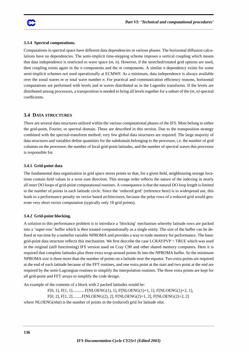
Part VI: ‘Technical and computational procedures’
n calcu-
means
d,
ailable
tal
are
o either
trategy
ority of
r of grid
ocessor
e loca-
nearly
mited
se, this
uld gen-
acked
e de-
basic
s used
e it is
imum
equired
end are
ept for
3.3.4 Spectral computations.
Computations in spectral space have different data dependencies in various phases. The horizontal diffusio
lations have no dependencies. The semi-implicit time-stepping scheme imposes a vertical coupling which
that data independence is restricted to wave space (m, n). However, if the stretched/rotated grid options are use
then coupling exists again in then components and them components. A similarn dependency exists for some
semi-implicit schemes not used operationally at ECMWF. As a minimum, data independence is always av
over the zonal wavesm or total wave numbern. For practical and communication efficiency reasons, horizon
computations are performed with levels andm waves distributed as in the Legendre transforms. If the levels
distributed among processors, a transposition is needed to bring all levels together for a subset of the(m, n)spectral
coefficients.
3.4 DATA STRUCTURES
There are several data structures utilized within the various computational phases of the IFS. Most belong t
the grid-point, Fourier, or spectral domain. These are described in this section. Due to the transposition s
combined with the spectral-transform method, very few global data structures are required. The large maj
data structures and variables define quantities for the subdomain belonging to the processor, i.e. the numbe
columns on the processor, the number of local grid-point latitudes, and the number of spectral waves this pr
is responsible for.
3.4.1 Grid-point data
The fundamental data organization in grid space stores points so that, for a given field, neighbouring storag
tions contain field values in a west–east direction. This storage order reflects the nature of the indexing in
all inner DO loops of grid-point computational routines. A consequence is that the natural DO loop length is li
to the number of points in each latitude circle. Since the ‘reduced grid’ (reference here) is in widespread u
leads to a performance penalty on vector based architectures, because the polar rows of a reduced grid wo
erate very short vector computation (typically only 18 grid points).
3.4.2 Grid-point blocking.
A solution to this performance problem is to introduce a ‘blocking’ mechanism whereby latitude rows are p
into a ‘super-row’ buffer which is then treated computationally as a single entity. The size of the buffer can b
fined at run time by a namelist variable NPROMA and provides a way to trade memory for performance. The
grid-point data structure reflects this mechanism. We first describe the case LCRAYPVP = TRUE which wa
in the original (still functioning) IFS version used on Cray C90 and other shared memory computers. Her
required that complete latitudes plus three extra wrap-around points fit into the NPROMA buffer. So the min
NPROMA size is three more than the number of points on a latitude near the equator. Two extra points are r
at the end of each latitude because of the FFT routines, and one extra point at the start and two point at the
required by the semi-Lagrangian routines to simplify the interpolation routines. The three extra points are k
all grid-point and FFT arrays to simplify the code design.
An example of the contents of a block with 2 packed latitudes would be:
F[0, 1], F[1, 1]............F[NLOENG(1), 1], F[NLOENG(1)+1, 1], F[NLOENG(1)+2, 1],
F[0, 2], F[1, 2].........F[NLOENG(2), 2], F[NLOENG(2)+1, 2], F[NLOENG(2)+2, 2]
where NLOENG(nlat) is the number of points in the (reduced) grid for latitudenlat.
136
IFS Documentation Cycle CY25r1 (Edited 2003)
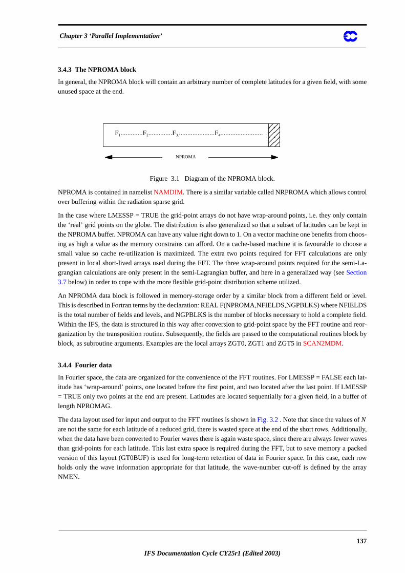
Chapter 3 ‘Parallel Implementation’
ome
l
ontain
kept in
hoos-
hoose a
only
mi-La-
vel.
DS
e field.
reor-
lock by
ch lat-
ESSP
ffer of
tionally,
er waves
packed
h row
array
3.4.3 The NPROMA block
In general, the NPROMA block will contain an arbitrary number of complete latitudes for a given field, with s
unused space at the end.
Figure 3.1 Diagram of the NPROMA block.
NPROMA is contained in namelistNAMDIM . There is a similar variable called NRPROMA which allows contro
over buffering within the radiation sparse grid.
In the case where LMESSP = TRUE the grid-point arrays do not have wrap-around points, i.e. they only c
the ‘real’ grid points on the globe. The distribution is also generalized so that a subset of latitudes can be
the NPROMA buffer. NPROMA can have any value right down to 1. On a vector machine one benefits from c
ing as high a value as the memory constrains can afford. On a cache-based machine it is favourable to c
small value so cache re-utilization is maximized. The extra two points required for FFT calculations are
present in local short-lived arrays used during the FFT. The three wrap-around points required for the se
grangian calculations are only present in the semi-Lagrangian buffer, and here in a generalized way (seeSection
3.7 below) in order to cope with the more flexible grid-point distribution scheme utilized.
An NPROMA data block is followed in memory-storage order by a similar block from a different field or le
This is described in Fortran terms by the declaration: REAL F(NPROMA,NFIELDS,NGPBLKS) where NFIEL
is the total number of fields and levels, and NGPBLKS is the number of blocks necessary to hold a complet
Within the IFS, the data is structured in this way after conversion to grid-point space by the FFT routine and
ganization by the transposition routine. Subsequently, the fields are passed to the computational routines b
block, as subroutine arguments. Examples are the local arrays ZGT0, ZGT1 and ZGT5 inSCAN2MDM.
3.4.4 Fourier data
In Fourier space, the data are organized for the convenience of the FFT routines. For LMESSP = FALSE ea
itude has ‘wrap-around’ points, one located before the first point, and two located after the last point. If LM
= TRUE only two points at the end are present. Latitudes are located sequentially for a given field, in a bu
length NPROMAG.
The data layout used for input and output to the FFT routines is shown inFig. 3.2. Note that since the values ofNare not the same for each latitude of a reduced grid, there is wasted space at the end of the short rows. Addi
when the data have been converted to Fourier waves there is again waste space, since there are always few
than grid-points for each latitude. This last extra space is required during the FFT, but to save memory a
version of this layout (GT0BUF) is used for long-term retention of data in Fourier space. In this case, eac
holds only the wave information appropriate for that latitude, the wave-number cut-off is defined by the
NMEN.
F1.............F2..............F3......................F4.........................
NPROMA
137
IFS Documentation Cycle CY25r1 (Edited 2003)
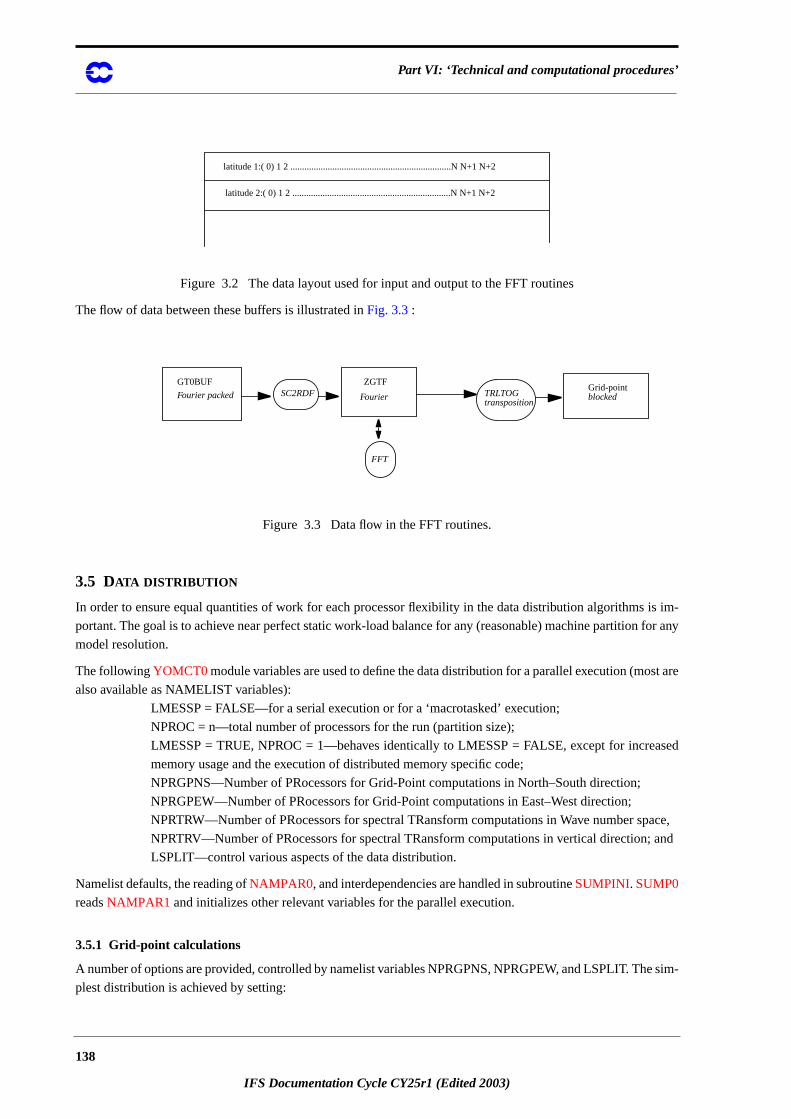
Part VI: ‘Technical and computational procedures’
is im-
for any
st are
sed
ace,
and
Figure 3.2 The data layout used for input and output to the FFT routines
The flow of data between these buffers is illustrated inFig. 3.3:
Figure 3.3 Data flow in the FFT routines.
3.5 DATA DISTRIBUTION
In order to ensure equal quantities of work for each processor flexibility in the data distribution algorithms
portant. The goal is to achieve near perfect static work-load balance for any (reasonable) machine partition
model resolution.
The followingYOMCT0 module variables are used to define the data distribution for a parallel execution (mo
also available as NAMELIST variables):
LMESSP = FALSE—for a serial execution or for a ‘macrotasked’ execution;
NPROC = n—total number of processors for the run (partition size);
LMESSP = TRUE, NPROC = 1—behaves identically to LMESSP = FALSE, except for increa
memory usage and the execution of distributed memory specific code;
NPRGPNS—Number of PRocessors for Grid-Point computations in North–South direction;
NPRGPEW—Number of PRocessors for Grid-Point computations in East–West direction;
NPRTRW—Number of PRocessors for spectral TRansform computations in Wave number sp
NPRTRV—Number of PRocessors for spectral TRansform computations in vertical direction;
LSPLIT—control various aspects of the data distribution.
Namelist defaults, the reading ofNAMPAR0, and interdependencies are handled in subroutineSUMPINI. SUMP0
readsNAMPAR1 and initializes other relevant variables for the parallel execution.
3.5.1 Grid-point calculations
A number of options are provided, controlled by namelist variables NPRGPNS, NPRGPEW, and LSPLIT. The sim-
plest distribution is achieved by setting:
latitude 1:( 0) 1 2 .....................................................................N N+1 N+2
latitude 2:( 0) 1 2 ....................................................................N N+1 N+2
GT0BUF
Fourier packed
ZGTF
FourierGrid-pointblocked
FFT
SC2RDF TRLTOGtransposition
138
IFS Documentation Cycle CY25r1 (Edited 2003)
Chapter 3 ‘Parallel Implementation’
ors and
ts ad-
urier
ced grid
lt.
d the
r grid-
titude
rangian
sors.
be more
istribu-
er split
orma-
l
d de-
st (see
row
ssors.
ber of
RV con-
h the
vels are
ut may
NPRGPEW =1
NPRGPNS = NPROC
LSPLIT = FALSE.
This option subdivides complete lines of latitude and complete sets of levels amongst available process
gives a good static load balance only for very specific values of NPROC for a particular model resolution. I
vantage lies in the fact that the data distribution is identical for the grid-point computations and for the Fo
transforms, thus eliminating the need for a transposition between these algorithmic stages. Use of the redu
with differing number of points for each latitude circle makes an even distribution of load particularly difficu
Setting LSPLIT=TRUE allows a line of latitude to be split so that part of it is assigned to one processor an
remainder is assigned to the next processor. This provides for a near perfect static work load distribution fo
point calculations, but the amount of parallelism remains limited by approximately 2/3 times the number of la
rows owing to the FFT and Legendre Transforms. There are also efficiency disadvantages in the semi-Lag
message passing because relatively more data has to be communicated to and from neighbouring proces
Another distribution type is achieved by setting:
NPRGPEW = n
NPRGPNS = m
where NPROC = n * m
It provides for considerable increased parallelism and allows the geographic area assigned to a processor to
‘square-shaped’, with consequent reduced communication volume in the semi-Lagrangian scheme. Data d
tion is first carried out in the north–south direction over NPRGPNS processors. Each sub-area is then furth
in the east–west direction over NPRGPEW processors (seeFigs. A.3 andA.4 ).
Because the static distribution employed is fully determined by the input namelist variables, all required inf
tion about distributions and communication patterns can be calculated in the setup phase.
SUMPand its descendentsSUMPLAT, SUSTAONLandSUSPLITLATcompute, among other things, the contro
structures which define the grid-point distributions.SUSTAONL is responsible for the grid-point distribution in
the east–west direction.
Scalars define the processor location (MYSETA, MYSETB) within the logical 2-dimensional processor gri
fined by NPRGPNS and NPRGPEW, where the A direction is north–south and the B direction is east–we
Fig. A.1).
For each processor in the A direction, the NFRSTLAT and NLSTLAT arrays define the first and last latitude
numbers allocated to that processor, and LSPLITLAT is TRUE for those latitudes which are split over 2 proce
NPTRLAT points to the start of each latitude. (SeeFig. A.2).
3.5.2 Fourier-space calculations
In order to retain good vector performance, it may be desirable to spread the latitudes over a different num
processors than that chosen for grid-point space. For this reason, separate variables NPRTRNS and NPRT
trol the data distribution, under the restriction that
NPROC = NPRTRNS x NPRTRV.
Achieving an even distribution of work north–south is a similar problem to that in grid-point space since, wit
reduced grid option, the number of Fourier waves are reduced as the poles are approached. Fields and le
combined together to create the vector dimension for the multiple FFT package (FFT992) used. Splitting this di-
mension across multiple processors is achieved by setting NPRTRV > 1. This will result in shorter vectors, b
139
IFS Documentation Cycle CY25r1 (Edited 2003)
Part VI: ‘Technical and computational procedures’
ected by
er the
UE. If
n grid-
ion.
pace
ach
much
ich ma-
essage
lled a
e con-
generic
appear
ctors of
ollowing
pies all
t be sent
or both
ions are
cally
be required when many processors are used. For cache-based computers the performance will not be aff
this splitting. Note that, if NPRGPEW is not 1, a transposition has to be performed in order to gather togeth
distributed portions of each latitude row needed as input to each FFT. This is also the case if LSPLIT=TR
NPRTRNS is not the same as NPRGPNS, the north–south distribution of rows or partial rows differs betwee
point computations and Fourier computations, resulting in a more complex transposition.
SubroutineSUMPLAT computes the Fourier-space data distribution. (SeeFig. A.2).
Array NULTPP—defines the number of latitudes for each processor in the north–south direct
Array NPTRLS—points to the first (global) latitude that each processor handles.
Array NPROCL—defines which processor computes the FFTs of that latitude.
Array NGPSET—contains the number of grid points which the processor owns, both in grid s
and in Fourier space.
Array NPTRLL(1: NPRTRV) points to the first level and NUMLL contains the number of levels owned by e
processor in the vertical decomposition.
3.6 DISTRIBUTED VECTORS
3.6.1 Introduction
Distributed vectors are widely used by subroutines which manipulate the analysis control vector, including
of the analysis and the Hessian singular vector code. They provide a convenient way to parallelize code wh
nipulates entire vectors rather than accessing individual elements. Their main advantage is that they hide m
passing from the user.
The basis of the parallelization method is the introduction into the IFS of a fortran 90 derived type ca
‘distributed_vector’. Variables of this type may be thought of as a pointers to one dimensional arrays whos
tents are spread over the available processors.
Fortran 90 allows the programmer to define what is meant by assignment, the arithmetic operators, and
functions, when they are applied to derived types. This feature has been used to allow distributed vectors to
in expressions and as arguments to the dot product routine. For example, if d1 and d2 are distributed ve
(say) 10000 elements each, and r1 is a one-dimensional array real array, also of 10000 elements, then the f
are legal fortran 90 statements:
r1(:) = d1
d1 = (3.0*d1 -5.5) / DOT_PRODUCT(d1,d2)
What is not immediately obvious is that both statements perform message passing. The first statement co
the elements of d1 into the array r1. Since many elements of d1 are stored on other processors, they mus
to the local processor. Similarly, the generic DOT_PRODUCT subroutine has been extended to allow one
arguments to be distributed vectors, in which case a parallel algorithm is used.
The second statement above illustrates another feature of distributed vector syntax. The arithmetic operat
written as if they apply to the whole vector. However, each processor will perform operations only on the lo
held part of the vector, thereby distributing the work.
3.6.2 Using distributed vectors
The following statement declares d1 and d2 to be distributed vectors:
TYPE (distributed_vector) :: d1,d2
140
IFS Documentation Cycle CY25r1 (Edited 2003)
Chapter 3 ‘Parallel Implementation’
pe
to deal-
tributed
ith real
same
al array
e, then
dimen-
the part
en the
h as the
ust be
e func-
s which
ines, see
, and to
etic op-
or this
vectors.
here r1
owing
y held
ments
essible
(Note that any of the usual qualifiers (INTENT, DIMENSION, ALLOCATABLE, etc.) may appear in the ty
statement.)
As with any pointer, we must allocate space for the data before we use a distributed vector, and remember
locate the space when we have finished with it. The following statements allocate and then deallocate a dis
vector of 10000 elements:
CALL allocate_vector (d1,10000)
CALL deallocate_vector (d1)
Once allocated, distributed vectors may appear in arithmetic expressions with other distributed vectors, w
scalars, or with one dimensional real arrays which are either of the same length as the full vector, or of the
length as the part of the vector which is held on the local processor. The result of such an expression is a re
of the size of the locally held part of the vector.
A distributed vector may appear on either side of an assignment statement. If it appears on the left hand sid
the right hand side must evaluate to a real scalar, to another distributed vector of the same length, to a one
sional real array of the same length as the full vector, or to a one dimensional array of the same length as
of the vector which is held locally. If the right hand side of an assignment statement is a distributed vector, th
left hand side must be either another distributed vector, or a real one dimensional array of the same lengt
full vector.
A distributed vector may appear as one argument of the DOT_PRODUCT function. The other argument m
either another distributed vector of the same length, or a real array of the same length as the full vector. Th
tions SUM and MAXVAL may also be called with distributed vector arguments.
A sub-vector may be extracted from a distributed vector into a local array using the function dvsection:
r(i:j) = dvsection (d1,i,j)
The routines gather_vector and scatter_vector may be used to copy between distributed vectors and array
are defined on a single processor (for example the IO processor). For examples of the use of these subrout
GETMINI andSAVMINI .
3.6.3 Optimizing distributed vector code
The overloaded assignment and arithmetic operators are intended to make it easy to convert existing code
make the parallelized code easy to read. However, it should be noted that each assignment and each arithm
eration results in a subroutine call. This is potentially expensive and inhibits some compiler optimizations. F
reason, an alternative syntax may be used to code frequently executed expressions involving distributed
This syntax is less elegant, but is more efficient. It is illustrated by the following example.
Consider the following statement, where d1 and d2 are distributed vectors of 10000 elements each, and w
is a one dimensional real array, also of 10000 elements:
d1 = d2 + r1(:)
This statement results in two subroutine calls: one for the addition and one for the assignment. The foll
statement is equivalent, but does not result in subroutine calls:
d1%local(:) = d2%local(:) + r1(d1%local_start:d1%local_end)
The notation is explained as follows. Each distributed vector is a structure containing a pointer to the locall
part of the vector, and three integers holding the full length of the vector and the indices of the first and last ele
of the locally held part. As illustrated in the example above, the components of a distributed vector are acc
using the "%" notation as (respectively) %local, %global_length, %local_start and %local_end.
141
IFS Documentation Cycle CY25r1 (Edited 2003)
Part VI: ‘Technical and computational procedures’
e par-
ure of
copying
ample:
cally
art of
rather
rs. The
porary
r that
ssible to
point
re point
ata held
ccessing
se data.
lled the
wind
re
bles
ors has
rs. De-
commu-
y also
e proc-
3.6.4 Warnings
There is an implicit assumption that statements involving distributed vectors will be executed by all PEs. B
ticularly careful in parallelizing IF statements. Care should also be taken in coding loops which use a mixt
distributed vectors and real arrays. It is easy to generate large amounts of message passing by frequent
between arrays and distributed vectors.
Another potential danger is a DOT_PRODUCT statement whose arguments are both expressions. For ex
dot = DOT_PRODUCT (d1+5.0 , d2-2.0)
This will not work as expected. Both "d1+5.0" and "d2-2.0" will evaluate to real arrays of the length of the lo
held part of d1 and d2. Each processor will apply the standard DOT_PRODUCT routine to its local p
"d1+5.0" and "d2-2.0" and each will calculate a different value for "dot".
This problem arises from the fact that the result of an expression involving a distributed vector is a real array
than a distributed vector. Unfortunately, it is not possible to make such expressions return distributed vecto
reason is rather subtle. Consider the following statement, where d1, d2 and d3 are distributed vectors:
d1 = (d2+d3)*d1 + (d2+d3)
The compiler will recognize that (d2+d3) is a common expression, and will generate code of the form:
temp = d2+d3
d1 = dtemp*d1 + temp
If arithmetic operations on distributed vectors returned distributed vectors, then the compiler-generated tem
vector temp would also be a distributed vector. Unfortunately, there is no way in fortran 90 to tell the compile
allocate_vector and deallocate_vector must be called when temp is created and destroyed. (It would be po
do this in an object-oriented language, such as C++.)
3.7 SEMI -LAGRANGIAN CALCULATION
3.7.1 Introduction
The semi-Lagrangian calculation in the IFS consists of two parts: the computation of a trajectory from a grid
backwards in time to determine the departure point; and the interpolation of various quantities at the departu
and at the mid point of the trajectory.
The issue for distributed memory computer systems is that both these parts require access to grid-point d
on neighbouring processors. For shared memory systems this issue can be resolved by processors simply a
data in the shared memory while, for distributed-memory systems, message passing is required to obtain the
The grid-column data that could potentially be required on a processor from neighbouring processors (ca
halo) is, in the present implementation, calculated assuming a conservative estimate of the global maximum
likely to be encountered (VMAX2 (m sec-1)) and the model time step TSTEP (s). Typical values for VMAX2 a
150–200 m sec-1. The advantage of using a fixed (large) VMAX2 is that semi-Lagrangian communication ta
can be calculated once and for all during the setup phase after the distribution of grid columns to process
been defined. This pre-fixed pattern then allows for efficient block transfers of halo data between processo
bugging is also easier than in a dynamic scheme. The disadvantage is that a large amount of the halo data
nicated may not really be required because the wind speed may be much lower than VMAX2. The wind ma
blow from the core region towards the edges of this processors domain, i.e. the departure point is within th
essor’s core region. The semi-Lagrangian communication tables are calculated by the subroutineSLRSETcalled
from SLCSET within SUSC2.
142
IFS Documentation Cycle CY25r1 (Edited 2003)
Chapter 3 ‘Parallel Implementation’
uous
orth–
on the
case
ed on
Once
essor
e only
g
on
tudes
iables
core
ive
tive
as a 1-
us halo
nner-
tly in
mi-La-
simple
d.
e are
orth
AX2
and
added
ation
When LMESSP is FALSE, the distribution of grid-point space to processors is done in partitions of contig
equally spaced latitudes, which allows the halo to be computed (inSUSC2) simply as a number of latitudes
(NSLWIDE) north and/or south of each processor partition.
However, when LMESSP is TRUE, the distribution of grid-point space is more general, supporting both n
south and east–west partitioning—in general a processor can have any continuous block of grid columns
sphere (seeFigs. A.6 andA.7 ). As a result, a processor’s halo cannot be expressed just by NSLWIDE. In this
SLCSETis called on each processor to calculate the halo of grid-point columns required by itself, bas
(VMAX2, TSTEP) and on the additional stencil requirements of the semi-Lagrangian interpolation method.
this is done,SLRSETis called to exchange this halo information with other processors so that each proc
knows what data need to be sent and received and which processors to communicate with. All this is don
once at initialization time.
Then during each model time step the SL halo is constructed by callingSLCOMM to perform the message passin
andSLEXTPOLto initialize those halo grid points that only require to be copied from other grid points held
the local processor. To simplify the interpolation routines, halo points are cyclically mirrored for complete lati
in the east–west direction, and mirror-extended near the poles.
3.7.2 SLCSET
SLCSETis called mainly to determine the SL halo for the local processor. This halo is described by array var
NSLSTA, NSLONL and NSLOFF, which are dimensioned by the number of latitudes that cover the halo and
region (seeFig. A.7) and are, briefly,
NSLSTA(JN)—starting (most westerly) grid point (relative to Greenwich) for halo on relat
latitude JN (is negative if the area starts west of Greenwich)
NSLONL(JN)—number of halo and core (i.e. belonging to this processor) grid points on rela
latitude JN
NSLOFF(JN)—offset from beginning of SL buffer to first halo grid point on relative latitude JN
The semi-Lagrangian buffer SLBUF1 contains the variables needed for semi-Lagrangian interpolation. It h
dimensional data structure representing the latitude fractions for each latitude within this processor’s core pl
region. The storage is organized from north towards south. The total size is calculated inSLCSETand called
NASLB1. To improve vector efficiency and cache performance the ‘horizontal’ collapsed dimension is the i
most loop in the semi-Lagrangian buffer. NASLB1 is just the container size and it may be increased sligh
SLCSETto avoid bank conflicts on vector machines. The second dimension represents the fields in the se
grangian buffer and will vary according to the chosen semi-Lagrangian configuration. This strategy makes it
to add new fields to the semi-Lagrangian buffer—no changes in the message-passing routines are neede
The calculation of the halo is done as follows:
For each latitude,
1) the minimum (i.e. most westerly) and maximum (i.e. most easterly) angles on the spher
determined for the local processor’s core region by considering NSLWIDE latitudes to the n
and south.
2) the angular distance a particle can travel on the sphere (given the maximum wind speed VM
and timestep TSTEP) is then subtracted and added respectively from the above minimum
maximum angles.
3) the angular distances are converted to grid points and at the same time a further grid point is
to satisfy the requirements of the interpolation method used. For more complex interpol
methods more points are required.
143
IFS Documentation Cycle CY25r1 (Edited 2003)
Part VI: ‘Technical and computational procedures’
grid
n the
the
the
alo. As
imme-
tines.
int
ccess.
ion
ere
has to
with,
the
in the
int
sor N
int
t entry
s the
needed
y such
olved in
a proc-
iting for
ed before
m an-
oc-
4) NSLSTA, NSLONL and NSLOFF are then updated for this latitude, such that the number of
points required for the halo and core region is never greater than the number of grid points o
whole latitude plus the extra points (IPERIOD) required for the interpolation. In addition,
NSLWIDE latitudes at the north and south poles are forced to require full latitudes to simplify
design.
To aid debugging, space is also reserved on each latitude for NSLPAD grid points east and west of the h
these points are initialized to huge(), any attempt to use this data in an interpolation routine will result in an
diate floating point exception, which can simplify the detection of programming errors in SL interpolation rou
NSLPAD is 0 by default.
Once the halo has been determined,SLCSETthen initializes NSLCORE to contain the position of each core po
in the SL buffer. This data structure is used during the semi-Lagrangian calculations every time step.
Finally NSLEXT is initialized, which is used to simplify a SL buffer (lat, lon) offset calculation inLASCAW. This
reduces an ‘IF TEST’ (to account for phase change over poles) and a ‘modulo function’, to a simple array a
As a resultLASCAW becomes more efficient and more maintainable.
3.7.3 SLRSET
SLRSETis called bySLCSETat initialization time to determine the detailed send- and receive-list informat
that will be used later bySLCOMM during model execution. This is achieved by a global communication wh
send and receive lists are exchanged in terms of global (LAT, LON) coordinates.
The data structures initialized bySLRSET are as follows (seeFig. A.7):
NSLPROCS is a scalar which defines the number of processors that the local processor
communicate with during SL halo communication.
Array NSLCOMM contains the list of processors that the local processor has to communicate
and is dimensioned 1: NSLPROCS.
Arrays NSENDNUM, NRECVNUM contain the number of send and receive (lat, lon) pairs that
local processor has to communicate. The difference between elements (N) and (N+1) conta
number of entries that apply to processor N.
Arrays NRLSTLAT, NRLSTLON describe the global latitude and longitude of the grid-po
columns to be received during SL halo communication. Columns to be received from proces
start at entry NRECVNUM(N) in these arrays.
Arrays NSLSTLAT, NSLSTLON describe the global latitude and longitude of the grid-po
columns to be sent during SL halo communication. Columns to be sent to processor N start a
NSENDNUM(N) in these arrays.
3.7.4 SLCOMM
SLCOMM is called at each model time step to obtain grid-point halo data from neighbouring processors. A
data volume for these communications can be very large, a strategy is used to control the amount of memory
for the message-passing mailbox. This is done by blocking the data to be sent and controlling how man
blocks can be queued in a processors mailbox. Control is achieved by recognising that processor pairs inv
SL communication send and receive a similar amounts of data, and by only sending the next block of data to
essor when a corresponding block has been received from that processor. With this approach we avoid wa
messages from processors that are still computing and use a probe function to detect if a message has arriv
issuing a receive for it. In this protocol, it is possible for 2 blocks to be queued at a destination processor fro
other processor. At initialization time (SLRSET) we compute the maximum number of processors that any pr
144
IFS Documentation Cycle CY25r1 (Edited 2003)
Chapter 3 ‘Parallel Implementation’
iven
ROC-
1).
d at a
count
icity and
fields
ciated
ection
l since
void
ubrou-
outine
essor has to communicate with (NSLPROCSMX), which is simply the maximum of NSLPROCS. G
NCOMBFLEN is the maximum number of words that we want to use at any processors mailbox and NSLP
SMX we can compute the maximum block size by NSLMPBUFSZ = NCOMBFLEN/(3*NSLPROCSMX–
Note that the factor 2*NSLPROCSMX corresponds to the maximum number of blocks that can be queue
processor’s mailbox for SL communication. The extra factor NSLPROCSMX–1 is needed to take into ac
mailbox fragmentation.
3.8 PROGRAM FLOW WITH THE FOCUS ON DISTRIBUTED -MEMORY DETAILS
3.8.1 Overview
The state variable of the model consists of the spectral components of the pseudo-divergence, pseudo-vort
surface pressure (or its logarithm) which gives 2*NFLEV+1 horizontal fields. In addition, we havep thermody-
namic variables andq dynamically-passive scalar variables. In the 1997 ECMWF operational model,p = 1 (R *
virtual temperature). Specific humidity is usually kept in grid-point space, where also three prognostic cloud
are used. No passive scalar variables are used in the model.
The size of the dynamical part of the state variable of the model is then:
(NSMAX+1)*(NSMAX+2)*((2+p+q)*NFLEV +1), where NSMAX is the degree of the truncation
and NFLEV the number of levels.
3.8.2 Constraints
The IFS has been designed to the following constraints:
1) it supports a direct integration, and also an adjoint and tangent-linear integration with asso
management of the trajectory—de facto there are three models in one;
2) it supports two- and three-time-level Lagrangian advection schemes and an Eulerian adv
scheme;
3) it supports a variable-resolution (reduced) grid;
4) the post-processing is built in;
5) possibility of a restart which gives the same result;
6) a normal-mode initialization process is included;
7) the Legendre functions and the normal modes are recomputed for each experiment (essentia
the geometry may vary);
8) coding conventions—DOCTOR norms are used;
9) message passing and macro-tasking with reproducibility;
10) flexible placement in memory during grid-point calculations and transforms, in order to a
memory bank conflicts;
11) message passing and macro-tasking intended to be performed at high level;
12) language—fixed format FORTRAN 90;
13) unification of the vertical interpolation routines;
14) the collocation grid is independent of the truncation.
The tangent-linear model and its adjoint are provided by coding the tangent linear and the adjoint of each s
tine. This is not the most efficient solution in terms of CPU but it is much easier to debug since it can be done r
by routine and the maintenance will obviously be greatly simplified.
Implicit in the following is the fact that we have three grid-point arrays (t–dt andt+dt, with only the fields, andt
145
IFS Documentation Cycle CY25r1 (Edited 2003)
Part VI: ‘Technical and computational procedures’
ectral
adjoint
ber in
RUE
he dis-
cause
ut-of-
E,
N,
de
with the fields plus their horizontal derivatives). For the integration of the model alone, we need only one sp
array (for the state variable), even considering the post-processing time steps. However during NMI and the
integration, we need a second one.
3.8.3 Computer code organization
Note: The physical package is taken in this part as a ‘black box’. Its input are fields at timet1 andt2 and its output
are fields at the same timest1 andt2, only those at timet2 being modified.
Here follows a description of the data and control flow. The displacement of the routine name and the num
square brackets indicate the nesting level within IFS.
• MAIN
• cnt0
• su0yoma
• sumpini
Read namelistNAMPAR0.
Determine if distributed-memory version or shared-memory version is used (LMESSP). If LMESSP is T
NMESS is defined to be 1, otherwise it is set to 0. NMESS is used to dimension some arrays used only in t
tributed-memory version.
Processors are logically divided in a 2D decomposition (NPRGPNS*NPRGPEWfor grid-point calculations and
NPRTRW*NPRTRV for Fourier and Legendre transforms). It is possible to supply onlyNPROC = (NPRG–PNS*NPRGPEWand NPRTRW*NPRTRV) and let the code decide how to make the 2D decomposition.
NPROCK is the number of processors to be used simultaneously to executeNUMKF Kalman filter forecasts.
Decide the amount of diagnostic output (NOUTPUT and LMPDIAG)
• su0dminit
• mpe_init
Initialize Message Passing Interface (MPI),
Determine MYPROC, A-set (MYSETA) and B-set (MYSETB)
• sulun
• sumpout
Based on NOUPUT determine which PE’s are writing diagnostics, the other PE’s do not write be
LOUTPUT = FALSE, or output data is dumped to /dev/null
• suarg
Read command line arguments and GRIB headers
• suct0
Define variables fixed at level zero. If LMESSP = TRUE we disable Cray macro-tasking and the use of ‘o
core’ work files (LCRAYPVP = FALSE, LMLTSK = FALSE, LIOXXX = FALSE)
• sump0
Set defaults forNAMPAR1 variables. These control the layout of data distribution (LSPLIT, LAPPL
NAPLAT), tuning communication for specific architectures (LSLSYNC, LBIDIR, NPHASE, NCOMBFLE
NLAGA, NLAGB, NVALAG, NCOSTLAG, NLAGBDY), control of I/O (NINSTR1, NINSTR2, NSTRIN,
NSTROUT, NFLDIN, NFLDOUT, LSPLITIN, LSPLITOUT), and for debugging semi-Lagrangian co
(NSLPAD)
Read NAMPAR1 namelist and initialize timing arrays
• sutag
146
IFS Documentation Cycle CY25r1 (Edited 2003)
Chapter 3 ‘Parallel Implementation’
ifferent
B.
n be
ainly
space,
nd
AX
(:),
rthern
tures.
ere a
grid-
. This
VN,
ASE
Set up separate communication tag ranges to be able to distinguish communication performed by d
message passing routines
• sumpi
Set up MPI identifiers (MINTET, MREALT, MLOGIT, MCHART).
• sudim
Calculate NFLEVL, NPSURF(), NPSP, NFLEVMX and NUMLL(), based on NFLEVG and NPROC
NPROMA is allowed to be any value greater than zero if LMESSP = TRUE
• suallo
Allocate arrays. At this point only distributed memory arrays based on NPROCA, NPROCB and NFLEVL ca
allocated.
• su0yomb
• sugem1a
Defines data structures for lat-long geometry that are independent of distributed memory configuration. M
NLOENG(NDGSAG: NDGENG) and NMENG(NDGSAG: NDGENG).
• sump
Master initialization routine for message-passing related data structures. Data distributions in grid-point
Fourier space and spectral space are defined.
• sualmp1
Allocate data structures to be defined insump. The data distributions are not yet defined, so only NPROCA/B a
NFLEVL can be used to determine dimensions.
• suwavedi
Determines partitioning of zonal wave numbers to PEs for all truncations involved (NSMAX, NCMAX, NTM
and NXMAX). Derived quantities are also calculated here (NASM0(:), NSPOLEGL, NPROCM(:), NUMPP
NSPEC, NSPEC2, NSPEC2MX, NPOSSP and IMYMS(:))
Back insumpNUMP is defined. Each PE calculates Legendre polynomials for a subset of latitudes in the no
hemisphere. The latitude distribution is determined here.
• sumplat
Calculate latitude distribution in grid-point space and Fourier space. Define a number of related data struc
• sustaonl
Define the grid-point columns that belong to this processor. This is most complex if NPROCB >1 wh
splitting in east–west direction is applied. The splitting depends on the LAPPLE and NAPLAT values. The
point column distribution on all other processors are communicated via message passing to this PE
information is stored in NSTA(: , :) and NONL(: , :).
• susplitlat
Defines variables that control the handling of the latitude split among A-set (LSNDS, LSNDN, LRCVS, LRC
NSNDS, NSNDN).
• sumpretr
Calculates MYSENDA(:) and MYRECVA(:) for recursive A-set transposition case. Values depend on NPH
• subidir
Calculates MYSENDA(:) and MYRECVA(:) for bi-directional communication case
• suallt
If it is a variational job allocate trajectory arrays, most dimensioned using NSPEC2.
• cnt3
• opdis
Generate an operator display. Only processor 1 writes status to theifs.stat file
• sualspa
147
IFS Documentation Cycle CY25r1 (Edited 2003)
Part VI: ‘Technical and computational procedures’
to other
IBEX
D and
hey are
ional
e
this
onal
tidal
Allocate SPA3(: , : , :) in case NCONF=1
• reresf
Read restart files if they are available. Fields are read in on processor 1 and the proper parts are distributed
processors. Both spectral fields, surface fields and upper-air grid-point fields are treated
• csta
• suinif
Read initial data files if restart files are not available
• [8] suspec
Initialize spectral fields
• [9] suspecb
Initialize 2D-model versions
• [9] suspecg
Initialize 3D-model versions. Spectral GRIB files are (usually) read on PE1 and decoded using the GR
subroutine. The correct spectral subsets are distributed to the other processors using MPE_SEN
MPE_RECV
• [10] gribex
GRIB decoding
• [10] suspgpg
If required some spectral fields (e.g. humidity) are transformed from spectral to grid point space because t
represented in grid point space in the state vector
• [9] suorog
Initialize grid-point orography and derivatives of orography from spectral-input orography. This is opt
because a grid-point orography might be available.
• [8] specrt
Calculate spectral coefficients of ‘TV’ (TV defined as RT/Rd) based on humidity and, if available, cloud liquid/ic
properties. Calculation for distributed memory version is done in the dm-code version.
• [9] specrtdm
Perform transforms of field to grid point space where RT/Rd is calculated.
• [11] gprcp
Calculates explicit normal modes (SPHBUF(:), HOUBUF(:)) for the zonal wave numbers treated by
processor, and frequencies required for tidal-wave initialization (FREQ(: , :), FREQ2(: , :)) for all NXPECG z
wave numbers.
• sumode3l
Calculate logical arrays defining Rossby and gravity modes LTYPGR(: , :), diabatic subset LTYPDB(: , :) ,
wave subset LTYPTD (: , :). They are dimensioned using the global NXPECG.
Optional writing of normal modes on external files (which is not done if LMESS = TRUE).
• sumode3i
Calculates implicit normal modes (RPINBUF(:) with dimensioning based on the local NCPEC).
• surinc
Initialize incremental variational job variables. No dependencies on distributed memory.
• sulcz
Initialize Lanczos common variables. No dependencies on distributed memory.
• sujbcov
Setup of the background error constraint JB. No dependencies on distributed memory.
• cnt1
• cnt2
148
IFS Documentation Cycle CY25r1 (Edited 2003)
Chapter 3 ‘Parallel Implementation’
to other
IBEX
hey are
onal
ated to
• suallt
If it is a variational job allocate trajectory arrays, most dimensioned using NSPEC2.
• cnt3
• opdis
Generate an operator display. Only processor 1 writes status to theifs.stat file
• sualspa
Allocate SPA3(: , : , :) in case NCONF=1.
• reresf
Read restart files if they are available. Fields are read in on processor 1 and the proper parts are distributed
processors. Both spectral fields, surface fields and upper air grid point fields are treated.
• csta
• uinif
Read initial data files if restart files are not available.
• [8] suspec
Initialize spectral fields.
• [9] suspecb
Initialize 2D-model versions.
• [9] suspecg
Initialize 3D-model versions. Spectral GRIB files are (usually) read on PE1 and decoded using the GR
subroutine. The correct spectral subsets are distributed to the other processors usingMPE_SEND and
MPE_RECV.
• [10] gribex
• [10] suspgpg
If required some spectral fields (e.g. humidity) are transformed from spectral to grid-point space because t
represented in grid-point space in the state vector.
• [9] suorog
Initialize grid-point orography and derivatives of orography from spectral-input orography. This is opti
because a grid-point orography might be available.
• [8] specrt
Calculate spectral coefficients of ‘TV’ (TV defined as RT/Rd) based on humidity and, if available, cloud liquid/ice
properties. Calculation for distributed memory version is done in the dm-code version.
• [10] specrtdm
Perform transforms of field to grid-point space where RT/Rd is calculated.
• [11] gprcp
• [10] gprcp
Calculate R based on humidity and, if available, cloud liquid/ice properties.
• spnorm
Calculate spectral norm diagnostics. Partial norm contributions are calculated on each PE and communic
PE1 (using the subroutinecommspnorm). On PE1 the global norms are calculated in a reproducible manner.
• cnmi
Normal-mode initialization.
• cmac
• fltmode
Projection onto subsets of normal modes.
• fltrg
Hough filter of increments
• edfi
149
IFS Documentation Cycle CY25r1 (Edited 2003)
Part VI: ‘Technical and computational procedures’
Controls integration for digital filter
• dealnmi
Deallocates arrays used in normal-mode calculations
• cnt4
Integration at level 4
• stepo
Basic time-stepping flow control
• [8] ltinvh
Inverse Legendre transforms
• [9] ltinvm
• [10] ltinv
• [11] asre1
Recombine symmetric and antisymmetric parts
• [12] asre1b
• [9] trmtol
Transposition from wave to Fourier space
• [8] scan2h
Multitasking interface to SCAN2M
• [9] scan2m
Computations in grid-point space
• [10] ftinvh
Control routine for inverse FFTs
• [11] ftinv
Inverse Fourier-transform driver
• [12] fft99
Fourier transform
• [11] trltog
Transposition from Fourier to grid-point space
• [10] cpg
Control of grid-point computations
• [11] gpxyb
Computes auxiliary arrays
• [11] gprh
Computes ES and RH from T and Q
• [11] lacdyn
Computation oft andt - dt at grid points
• [11] cpcuddh
DDH accumulation
• [11] cpdyddh
Calculation of variables and dynamical flux-tendency diagnostics for DDH
• [11] gprcp
Computes CP, R and R/CP from Q
• [10] slcomm
Semi-Lagrangian halo communications
• [10] raddrv
Control of radiation calculations
150
IFS Documentation Cycle CY25r1 (Edited 2003)
Chapter 3 ‘Parallel Implementation’
e
north–
W. The
• [10] cpglag
Lagged grid-point computations
• [11] lapine
Interface for Semi-Lagrangian interpolations
• [11] callpar
Interface for ECMWF Physics package
• [11] postphy
Post Physics computations
• [11] gpendtr
Final memory transfers incpglag
• [11] gppref
Compute full-level pressure
• [11] sc2rdg
Copy grid-point arrays from buffer
• [10] ftdirh
Control for Fourier transforms
• [11] trgtol
Transposition from grid-point to Fourier space
• [8] ltdirh
Control for direct Legendre transforms
• [9] trltom
Transposition from Fourier to spectral wave space
• [9] ltdirm
• [10] ltdir
Legendre transforms
• [8] spch
Control spectral-space calculations
• [10] trmtos
Transposition from horizontal to vertical spectral coefficients
• [10] trstom
Transposition from vertical to horizontal spectral coefficients
• spnorm
Compute spectral norms
• comtim
Parallel-processing timing.
APPENDIX A D ESCRIPTIONS OF DATA STRUCTURES
Extensive use is made in the code of a set of scalar integers held in moduleYOMMP. These are used to assist th
description of the data partitioning across processors and are based on the strategy of first partitioning in the
south direction (NPRGPNS) and then further subpartitioning east–west, according to the value of NPRGPE
subdivision in each dimension is called a SET, leading to:
MYSETA: subdivision of latitudes in N–S direction, where MYSETA = 1..NPRGPNS
MYSETB: subdivision of latitudes in E–W direction, where MYSETB = 1..NPRGPEW
Similarly, for the wave-space partitioning:
MYSETW: subdivision of meridional waves, where MYSETW = 1..NPRTRW
151
IFS Documentation Cycle CY25r1 (Edited 2003)
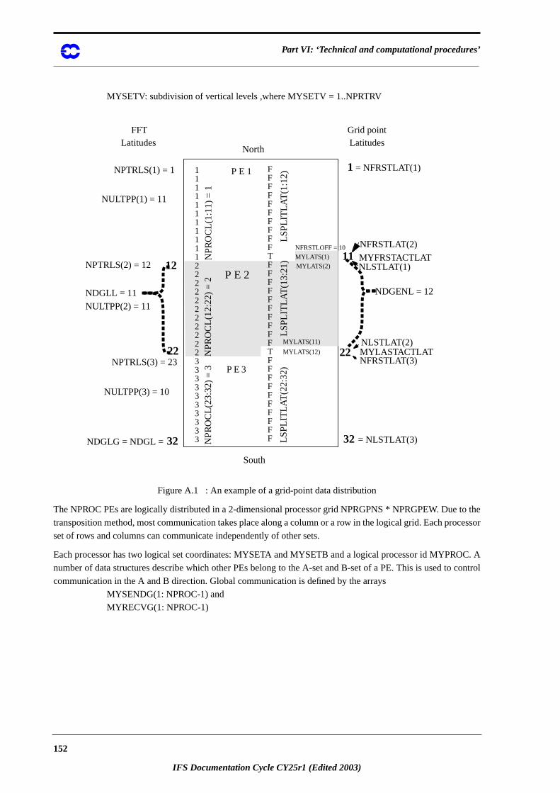
Part VI: ‘Technical and computational procedures’
to the
cessor
C. A
control
MYSETV: subdivision of vertical levels ,where MYSETV = 1..NPRTRV
Figure A.1 : An example of a grid-point data distribution
The NPROC PEs are logically distributed in a 2-dimensional processor grid NPRGPNS * NPRGPEW. Due
transposition method, most communication takes place along a column or a row in the logical grid. Each pro
set of rows and columns can communicate independently of other sets.
Each processor has two logical set coordinates: MYSETA and MYSETB and a logical processor id MYPRO
number of data structures describe which other PEs belong to the A-set and B-set of a PE. This is used to
communication in the A and B direction. Global communication is defined by the arrays
MYSENDG(1: NPROC-1) and
MYRECVG(1: NPROC-1)
FFFFFFFFFFTFFFFFFFFFFTFFFFFFFFFF
11111111111222222222223333333333
North
South
NFRSTLOFF = 10
MYLATS(1)
MYLATS(2)
NP
RO
CL(
1:11
) =
1N
PR
OC
L(12
:22)
= 2
NP
RO
CL(
23:3
2) =
3
P E 1
P E 2LS
PLI
TLA
T(1
:12)
LSP
LIT
LAT
(13:
21)
LSP
LIT
LAT
(22:
32)P E 3
MYLATS(11)
MYLATS(12)
1 = NFRSTLAT(1)
11NFRSTLAT(2)
NLSTLAT(1)MYFRSTACTLAT
NDGENL = 12
22NLSTLAT(2)MYLASTACTLATNFRSTLAT(3)
Grid pointLatitudes
32 = NLSTLAT(3)
12
22
NPTRLS(2) = 12
NPTRLS(3) = 23
NDGLG = NDGL = 32
NDGLL = 11
NULTPP(2) = 11
NULTPP(1) = 11
NULTPP(3) = 10
NPTRLS(1) = 1
FFTLatitudes
152
IFS Documentation Cycle CY25r1 (Edited 2003)
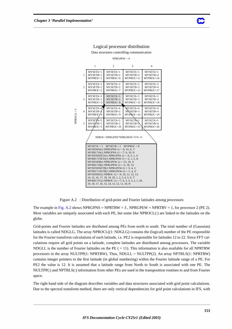
Chapter 3 ‘Parallel Implementation’
.
on the
ssian)
sible
T cal-
ariable
W)
. For
E. The
ourier
lations.
, with
Figure A.2 : Distribution of grid-point and Fourier latitudes among processors
The example inFig. A.2shows NPRGPNS = NPRTRW = 3 , NPRGPEW = NPRTRV = 1, for processor 2 (PE 2)
Most variables are uniquely associated with each PE, but some like NPROCL(:) are linked to the latitudes
globe.
Grid-points and Fourier latitudes are disributed among PEs from north to south. The total number of (Gau
latitudes is called NDGLG. The array NPROCL((1: NDGLG) contains the (logical) number of the PE respon
for the Fourier transform calculations of each latitude, i.e. PE2 is responsible for latitudes 12 to 22. Since FF
culations require all grid points on a latitude, complete latitudes are distributed among processors. The v
NDGLL is the number of Fourier latitudes on the PE ( = 11). This information is also available for all NPRTRW
processors in the array NULTPP(1: NPRTRW). Thus, NDGLL = NULTPP(2). An array NPTRLS(1: NPRTR
contains integer pointers to the first latitude (in global numbering) within the Fourier latitude range of a PE
PE2 the value is 12. It is assumed that a latitude range from North to South is associated with one P
NULTPP(:) and NPTRLS(:) information from other PEs are used in the transposition routines to and from F
space.
The right hand side of the diagram describes variables and data structures associated with grid point calcu
Due to the spectral transform method, there are only vertical dependencies for grid point calculations in IFS
NPROC=NPRGPNS*NPRGPEW=5*4= 0
1 2 3 4
1MYSETA=1MYSETB=1MYPROC=1
MYSETA=1MYSETB=2MYPROC=6
MYSETA=1MYSETB=3
MYPROC=11
MYSETA=1MYSETB=4
MYPROC=16
2MYSETA=2MYSETB=1MYPROC=2
MYSETA=2MYSETB=2MYPROC=7
MYSETA=2MYSETB=3
MYPROC=12
MYSETA=2MYSETB=4
MYPROC=17
3MYSETA=3MYSETB=1MYPROC=3
MYSETA=3MYSETB=2MYPROC=8
MYSETA=3MYSETB=3
MYPROC=13
MYSETA=3MYSETB=4
MYPROC=18
4MYSETA=4MYSETB=1MYPROC=4
MYSETA=4MYSETB=2MYPROC=9
MYSETA=4MYSETB=3
MYPROC=14
MYSETA=4MYSETB=4
MYPROC=19
5MYSETA=5MYSETB=1MYPROC=5
MYSETA=5MYSETB=2
MYPROC=10
MYSETA=5MYSETB=3
MYPROC=15
MYSETA=5MYSETB=4
MYPROC=20
MYSETA = 3 MYSETB = 2 MYPROC = 8MYSENDA(1:NPRGPNS-1) = /9, 10, 6, 7/MYRECVA(1:NPRGPNS-1) = /7, 6, 10, 9/MYSENDSETA(1:NPRGPNS-1) = /4, 5, 1, 2/MYRECVSETA(1:NPRGPNS-1) = /2, 1, 5, 4/MYSENDB(1:NPRGPEW-1) = /13, 18, 3/MYRECVB(1:NPRGPEW-1) = /3, 18, 13/MYSENDSETB(1:NPRGPEW-1) = /3, 4, 1/MYRECVSETB(1:NPRGPEW-1) = /1, 4, 3/MYSENDG(1:NPROC-1) = /9, 10, 11, 12, 13,14, 15, 16, 17, 18, 19, 20, 1, 2, 3, 4, 5, 6, 7/MYRECVG(1:NPROC-1) = /7, 6, 5, 4, 3, 2, 1, 20,19, 18, 17, 16, 15, 14, 13, 12, 11, 10, 9/
NP
RO
CA
= 5
Logical processor distributionData structures controlling communication
NPRGPEW = 4
153
IFS Documentation Cycle CY25r1 (Edited 2003)
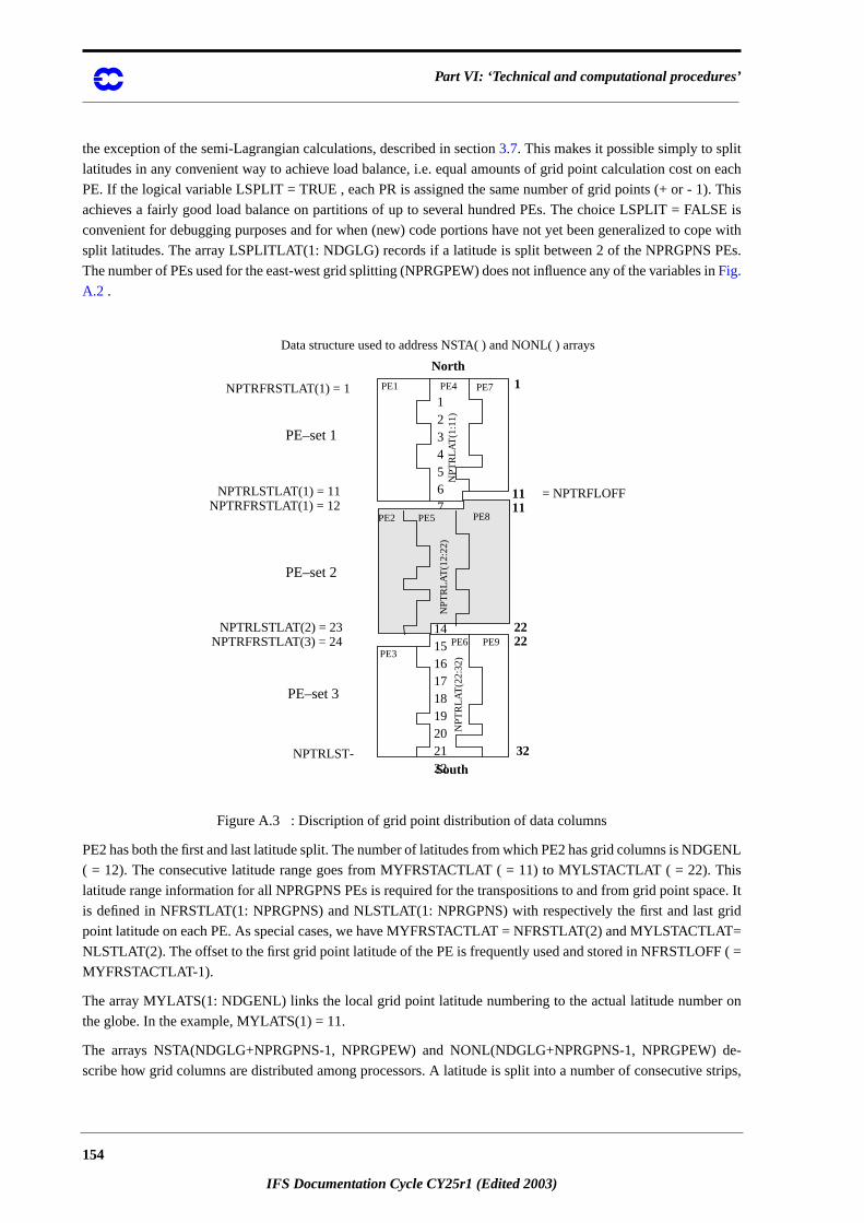
Part VI: ‘Technical and computational procedures’
n each
. This
SE is
pe with
PEs.
in
GENL
ace. It
grid
T=
F ( =
r on
de-
strips,
the exception of the semi-Lagrangian calculations, described in section3.7. This makes it possible simply to split
latitudes in any convenient way to achieve load balance, i.e. equal amounts of grid point calculation cost o
PE. If the logical variable LSPLIT = TRUE , each PR is assigned the same number of grid points (+ or - 1)
achieves a fairly good load balance on partitions of up to several hundred PEs. The choice LSPLIT = FAL
convenient for debugging purposes and for when (new) code portions have not yet been generalized to co
split latitudes. The array LSPLITLAT(1: NDGLG) records if a latitude is split between 2 of the NPRGPNS
The number of PEs used for the east-west grid splitting (NPRGPEW) does not influence any of the variablesFig.
A.2 .
Figure A.3 : Discription of grid point distribution of data columns
PE2 has both the first and last latitude split. The number of latitudes from which PE2 has grid columns is ND
( = 12). The consecutive latitude range goes from MYFRSTACTLAT ( = 11) to MYLSTACTLAT ( = 22). This
latitude range information for all NPRGPNS PEs is required for the transpositions to and from grid point sp
is defined in NFRSTLAT(1: NPRGPNS) and NLSTLAT(1: NPRGPNS) with respectively the first and last
point latitude on each PE. As special cases, we have MYFRSTACTLAT = NFRSTLAT(2) and MYLSTACTLA
NLSTLAT(2). The offset to the first grid point latitude of the PE is frequently used and stored in NFRSTLOF
MYFRSTACTLAT-1).
The array MYLATS(1: NDGENL) links the local grid point latitude numbering to the actual latitude numbe
the globe. In the example, MYLATS(1) = 11.
The arrays NSTA(NDGLG+NPRGPNS-1, NPRGPEW) and NONL(NDGLG+NPRGPNS-1, NPRGPEW)
scribe how grid columns are distributed among processors. A latitude is split into a number of consecutive
12345678910111213141516171819202122
PE6
PE4PE1 PE7
PE9
PE2 PE5 PE8
PE3
NPTRFRSTLAT(1) = 1
NPTRLSTLAT(1) = 11NPTRFRSTLAT(1) = 12
NPTRLSTLAT(2) = 23NPTRFRSTLAT(3) = 24
NPTRLST-
PE–set 3
PE–set 1
PE–set 2
1
32
1111
= NPTRFLOFF
Data structure used to address NSTA( ) and NONL( ) arrays
North
South
NP
TR
LAT
(1:1
1)N
PT
RLA
T(1
2:22
)
NP
TR
LAT
(22:
32)
2222
154
IFS Documentation Cycle CY25r1 (Edited 2003)
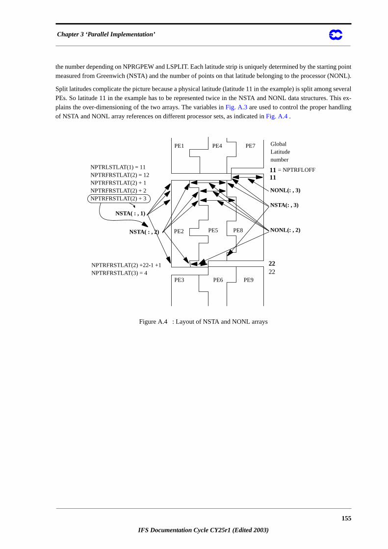
Chapter 3 ‘Parallel Implementation’
point
ONL).
several
his ex-
g
the number depending on NPRGPEW and LSPLIT. Each latitude strip is uniquely determined by the starting
measured from Greenwich (NSTA) and the number of points on that latitude belonging to the processor (N
Split latitudes complicate the picture because a physical latitude (latitude 11 in the example) is split among
PEs. So latitude 11 in the example has to be represented twice in the NSTA and NONL data structures. T
plains the over-dimensioning of the two arrays. The variables inFig. A.3 are used to control the proper handlin
of NSTA and NONL array references on different processor sets, as indicated inFig. A.4.
Figure A.4 : Layout of NSTA and NONL arrays
PE2 PE5 PE8
NONL(: , 3)
NSTA(: , 3)
NONL(: , 2)
NPTRLSTLAT(1) = 11NPTRFRSTLAT(2) = 12NPTRFRSTLAT(2) + 1NPTRFRSTLAT(2) + 2NPTRFRSTLAT(2) + 3
NSTA( : , 1)
NSTA( : , 2)
NPTRFRSTLAT(2) +22-1 +1NPTRFRSTLAT(3) = 4
PE1 PE4 PE7
PE3 PE6 PE9
GlobalLatitudenumber
1111
2222
= NPTRFLOFF
155
IFS Documentation Cycle CY25r1 (Edited 2003)
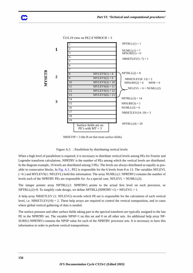
Part VI: ‘Technical and computational procedures’
er and
ibuted.
as pos-
VL
of
r, so
rtical
cases
the last
y NP-
ve this
Figure A.5 : Parallelism by distributing vertical levels
When a high level of parallelism is required, it is necessary to distribute vertical levels among PEs for Fouri
Legendre transform calculations. NPRTRV is the number of PEs among which the vertical levels are distr
In the diagram example, 19 levels are distributed among 3 PEs. The levels are always distributed as equally
sible in consecutive blocks. InFig. A.5 , PE2 is responsible for the 6 levels from 8 to 13. The variables NFLE
( =6 ) and MYLEVS(1: NFLEVL) hold this information. The array NUMLL(1: NPRTRV) contains the number
levels each of the NPRTRV PEs are responsible for. As a special case, NFLEVL = NUMLL(2).
The integer pointer array NPTRLL(1: NPRTRV) points to the actual first level on each processo
NPTRLL(2)=8. To simplify code design, we define NPTRLL(NPRTRV+1) = NFLEVG + 1.
A help array NBSETLEV (1: NFLEVG) records which PE-set is responsible for the calculation of each ve
level, i.e. NBSETLEV(10) = 2. These help arrays are required to control the vertical transposition, and in
where global vertical gathering of data is needed.
The surface pressure and other surface fields taking part in the spectral transform are typically assigned to
PE in the NPRTRV set. The variable NPSP=1 on this set and 0 on all other sets. An additional help arra
SURF(1:NPRTRV) contains the NPSP value for each of the NPRTRV processor sets. It is necessary to ha
information in order to perform vertical transpositions.
1
2
3
4
5
6
7
8 MYLEVS(1) = 8
9 MYLEVS(2) = 9
10 MYLEVS(3) = 10
11 MYLEVS(4) = 11
12 MYLEVS(5) = 12
13 MYLEVS(6) = 13
14
15
16
17
18
19
NPTRLL(1) = 1
NUMLL(1) = 7NPSURF(1) = 0
NBSETLEV(1: 7) = 1
NPTRLL(2) = 8
NPSURF(2) = 0 NPSP = 0
NFLEVL = 6 = NUMLL(2)
NPTRLL(3) = 14
NPSURF(3) = 1
NUMLL(3) = 6
MY
SE
TB
3
1
2
Surface fields are onPE’s with MT = 3
NBSETSP = 3 (the B-set that treats surface fields)
T21L19 view on PE2 if NPROCB = 3
NPTRLL(4) = 20
NBSETLEV(14: 19) = 3
NBSETLEV(8: 13) = 2
1
156
IFS Documentation Cycle CY25r1 (Edited 2003)
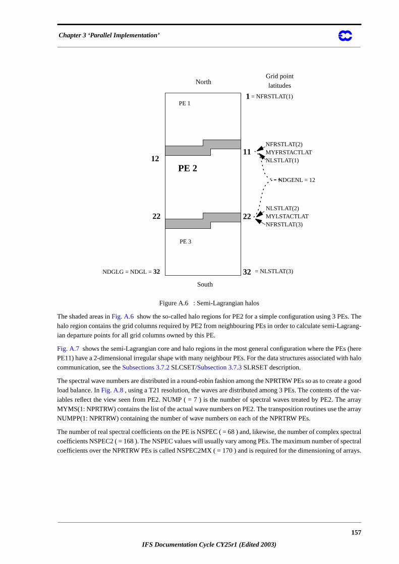
Chapter 3 ‘Parallel Implementation’
The
grang-
s (here
ith halo
e a good
e var-
ay
array
pectral
ectral
rrays.
Figure A.6 : Semi-Lagrangian halos
The shaded areas inFig. A.6 show the so-called halo regions for PE2 for a simple configuration using 3 PEs.
halo region contains the grid columns required by PE2 from neighbouring PEs in order to calculate semi-La
ian departure points for all grid columns owned by this PE.
Fig. A.7 shows the semi-Lagrangian core and halo regions in the most general configuration where the PE
PE11) have a 2-dimensional irregular shape with many neighbour PEs. For the data structures associated w
communication, see theSubsections 3.7.2 SLCSET/Subsection 3.7.3 SLRSET description.
The spectral wave numbers are distributed in a round-robin fashion among the NPRTRW PEs so as to creat
load balance. InFig. A.8 , using a T21 resolution, the waves are distributed among 3 PEs. The contents of th
iables reflect the view seen from PE2. NUMP ( = 7 ) is thenumber of spectral waves treated by PE2. The arr
MYMS(1: NPRTRW) contains the list of the actual wave numbers on PE2. The transposition routines use the
NUMPP(1: NPRTRW) containing the number of wave numbers on each of the NPRTRW PEs.
The number of real spectral coefficients on the PE is NSPEC ( = 68 ) and, likewise, the number of complex s
coefficients NSPEC2 ( = 168 ). The NSPEC values will usually vary among PEs. The maximum number of sp
coefficients over the NPRTRW PEs is called NSPEC2MX ( = 170 ) and is required for the dimensioning of a
North
South
PE 1
PE 2
PE 3
32
1211
1
2222
= NFRSTLAT(1)
NFRSTLAT(2)MYFRSTACTLATNLSTLAT(1)
NLSTLAT(2)MYLSTACTLATNFRSTLAT(3)
NDGENL = 12
= NLSTLAT(3)NDGLG = NDGL =32
Grid point
latitudes
157
IFS Documentation Cycle CY25r1 (Edited 2003)
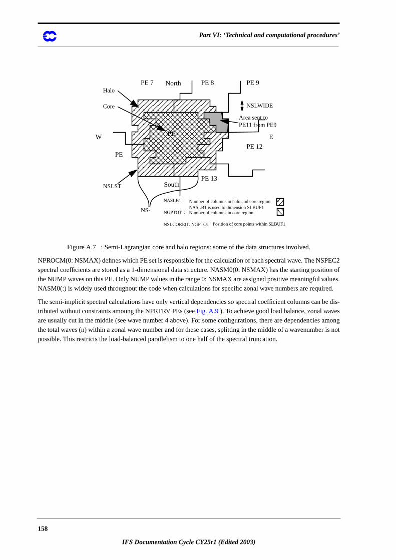
Part VI: ‘Technical and computational procedures’
PEC2
ition of
alues.
ired.
be dis-
s
s among
r is not
Figure A.7 : Semi-Lagrangian core and halo regions: some of the data structures involved.
NPROCM(0: NSMAX) defines which PE set is responsible for the calculation of each spectral wave. The NS
spectral coefficients are stored as a 1-dimensional data structure. NASM0(0: NSMAX) has the starting pos
the NUMP waves on this PE. Only NUMP values in the range 0: NSMAX are assigned positive meaningful v
NASM0(:) is widely used throughout the code when calculations for specific zonal wave numbers are requ
The semi-implicit spectral calculations have only vertical dependencies so spectral coefficient columns can
tributed without constraints amoung the NPRTRV PEs (seeFig. A.9 ). To achieve good load balance, zonal wave
are usually cut in the middle (see wave number 4 above). For some configurations, there are dependencie
the total waves (n) within a zonal wave number and for these cases, splitting in the middle of a wavenumbe
possible. This restricts the load-balanced parallelism to one half of the spectral truncation.
PE 12
PE 7 PE 8 PE 9
PE
PE
PE 13
Core
Area sent toPE11 from PE9
Halo
NSLST
NS-
NSLWIDE
W
South
North
E
NASLB1 :
NGPTOT :
NSLCORE(1: NGPTOT
Number of columns in halo and core regionNASLB1 is used to dimension SLBUF1Number of columns in core region
Position of core points within SLBUF1
158
IFS Documentation Cycle CY25r1 (Edited 2003)
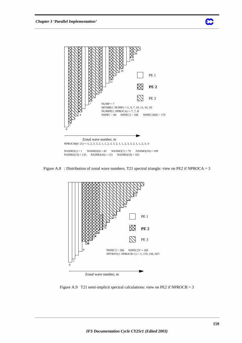
Chapter 3 ‘Parallel Implementation’
Figure A.8 : Distribution of zonal wave numbers. T21 spectral triangle: view on PE2 if NPROCA = 3
Figure A.9 T21 semi-implicit spectral calculations: view on PE2 if NPROCB = 3
0
13
1
4
7
19
10
16
PE 1
PE 2
PE 3
Zonal wave number, m
NUMP = 7MYMB(1: NUMP) = /1, 4, 7, 10, 13, 16, 19/NUMPP(1: NPROCA) = /7, 7, 8/NSPEC = 84 NSPEC2 = 168 NSPEC2MX = 170
NPROCM(0: 21) = /1, 2, 3, 3, 2, 1, 1, 2, 3, 3, 2, 1, 1, 2, 3, 3, 2, 1, 1, 2, 3, 3/
NASMO(1) = 1 NASMO(4) = 43 NASMO(7) = 79 NASMO(10) = 109NASMO(13) = 133 NASMO(16) = 151 NASMO(19) = 163
10
0
1
4
7
19
13
16
PE 3
PE 1
PE 2
Zonal wave number, m
NSPEC2 = 506 NSPEC2V = 169NPTRSV(1: NPROCB+1) = /1, 170, 339, 507/
159
IFS Documentation Cycle CY25r1 (Edited 2003)
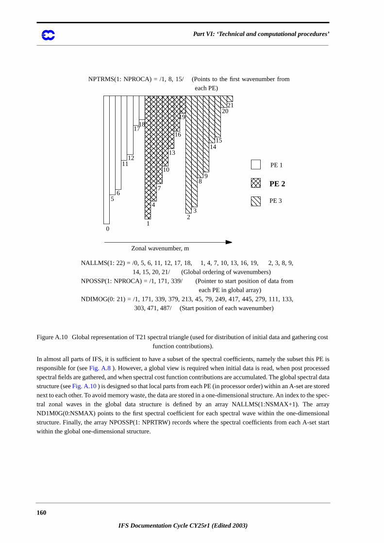
Part VI: ‘Technical and computational procedures’
cost
s PE is
ssed
tral data
tored
e spec-
rray
ional
et start
Figure A.10 Global representation of T21 spectral triangle (used for distribution of initial data and gathering
function contributions).
In almost all parts of IFS, it is sufficient to have a subset of the spectral coefficients, namely the subset thi
responsible for (seeFig. A.8 ). However, a global view is required when initial data is read, when post proce
spectral fields are gathered, and when spectral cost function contributions are accumulated. The global spec
structure (seeFig. A.10) is designed so that local parts from each PE (in processor order) within an A-set are s
next to each other. To avoid memory waste, the data are stored in a one-dimensional structure. An index to th
tral zonal waves in the global data structure is defined by an array NALLMS(1:NSMAX+1). The a
ND1M0G(0:NSMAX) points to the first spectral coefficient for each spectral wave within the one-dimens
structure. Finally, the array NPOSSP(1: NPRTRW) records where the spectral coefficients from each A-s
within the global one-dimensional structure.
01
23
45
67
89
1011
1213
1415
1617
1819
2021
PE 1
PE 3
PE 2
Zonal wavenumber, m
NALLMS(1: 22) = /0, 5, 6, 11, 12, 17, 18, 1, 4, 7, 10, 13, 16, 19, 2, 3, 8, 9,
14, 15, 20, 21/ (Global ordering of wavenumbers)
NPOSSP(1: NPROCA) = /1, 171, 339/ (Pointer to start position of data from
each PE in global array)
NDIMOG(0: 21) = /1, 171, 339, 379, 213, 45, 79, 249, 417, 445, 279, 111, 133,
303, 471, 487/ (Start position of each wavenumber)
NPTRMS(1: NPROCA) = /1, 8, 15/ (Points to the first wavenumber from
each PE)
160
IFS Documentation Cycle CY25r1 (Edited 2003)
IFS Documentation Cycle CY25r1
161
IFS Documentationn Cycle CY25r1 (Edited 2003)
REFERENCES
Andersson, E. and Courtier, Ph., 1992: Post-processing changes for IFS cycle 9. (Research Department memoran-
dum, internal note).
El Khatib, R.,1997: FULL-POS users’ guide in ARPEGE/IFS cycle 16T1_al07 and ALADIN cycle AL07 with
ARPEGE/IFS cycle 16T1_al07 (internal note).
Estrade J.-F., 1997: Développement ARPEGE/ALADIN. Mémoire distribuée/ mémoire partagée (internal note in
French).
Rochas, M. and Courtier, Ph.,1992: La méthode spectrale en météorologie. Note de travail ARPEGE numéro30,
58pp.
Undén, P.,1995: IFS post-processing changes proposed by METEO-FRANCE and an improved formulation (in-
ternal note).
Yessad, K., 1997: Semi-Lagrangian computations in the cycles 17 and 18 of ARPEGE/IFS (internal note).
Yessad, K., 1997: Semi-implicit spectral computations in the cycles 17 and 18 of ARPEGE/IFS (internal note).
Yessad, K., 1997: Horizontal diffusion in the cycles 17 and 18 of ARPEGE/IFS (internal note).
Yessad, K., 1997: Spectral transforms in the cycles 17 and 18 of ARPEGE/IFS (internal note).
Yessad, K.,1997: Sphere to sphere transforms in spectral space in the cycles 17 and 18 of ARPEGE/IFS: configu-
rations 911 and 912, TRAGEO. (internal note).
‘’
162
IFS Documentation Cycle CY25r1 (Edited 2003)