Identify Experts through Revealed Confidence: Application toWisdom of Crowds

by

Yunhao Zhang

B.A., University of California-Berkeley (2016)

Submitted to the THE SLOAN SCHOOL OF MANAGEMENTin partial fulfillment of the requirements for the degree of

MASTER OF SCIENCE IN MANAGEMENT RESEARCH

at the

MASSACHUSETTS INSTITUTE OF TECHNOLOGY

September 2020

© Massachusetts Institute of Technology 2020. All rights reserved.

Author . . . . . . . . . . . . . . . . . . . . . . . . . . . . . . . . . . . . . . . . . . . . . . . . . . . . . . . . . . . . . . . . . . .Department of Management

August 7, 2020

Certified by . . . . . . . . . . . . . . . . . . . . . . . . . . . . . . . . . . . . . . . . . . . . . . . . . . . . . . . . . . . . . . .Drazen Prelec

Digital Equipment Corp. Leader for Global Operations Professor of ManagementProfessor of Management Science and Economics

Thesis Supervisor

Accepted by . . . . . . . . . . . . . . . . . . . . . . . . . . . . . . . . . . . . . . . . . . . . . . . . . . . . . . . . . . . . . .Catherine Tucker

Sloan Distinguished Professor of ManagementProfessor, Marketing

Identify Experts through Revealed Confidence: Application to Wisdom of

Crowds

by

Yunhao Zhang

Submitted to the THE SLOAN SCHOOL OF MANAGEMENTon August 7, 2020, in partial fulfillment of the

requirements for the degree ofMASTER OF SCIENCE IN MANAGEMENT RESEARCH

AbstractWe propose our Revealed Confidence (RC) algorithm that improves Wisdom of Crowds (WoC)by identifying experts from the crowds. We highlight the important distinction between first- andsecond-order uncertainty, which also serves as an explanation for rational overconfidence. Underour proposed belief updating mechanism, we analyze the performance of RC algorithm and showthe algorithm could identify the more accurate prior estimates even if all agents report the sameprior confidence under conventional confidence elicitation, e.g. confidence interval. Our empiricalanalysis shows that (1) RC improves upon other Wisdom of Crowds methods by overweighting themore accurate agents in the aggregation (2) verifies one key prediction of our theoretical result thatthe distance effect indeed affects belief-updating henceforth RC algorithm’s performance, whichshould be carefully controlled for in order to optimize the algorithm.

Thesis Supervisor: Drazen PrelecTitle: Digital Equipment Corp. Leader for Global Operations Professor of ManagementProfessor of Management Science and Economics

2

Contents

1 Introduction 5

2 Rational Overconfidence & Higher-order Uncertainty 8

2.1 The Coin Example . . . . . . . . . . . . . . . . . . . . . . . . . . . . . . . . . . 8

3 The Revealed Confidence Algorithm 11

4 Updating Mechanism 14

4.1 Identification of Relative Expertise & the Distance Effect . . . . . . . . . . . . . . 15

4.2 Second-order Uncertainty . . . . . . . . . . . . . . . . . . . . . . . . . . . . . . . 16

5 Empirical Analysis 21

5.1 Method . . . . . . . . . . . . . . . . . . . . . . . . . . . . . . . . . . . . . . . . 21

5.1.1 Participants . . . . . . . . . . . . . . . . . . . . . . . . . . . . . . . . . . 21

5.1.2 Influence Selection . . . . . . . . . . . . . . . . . . . . . . . . . . . . . . 22

5.1.3 RC Estimate . . . . . . . . . . . . . . . . . . . . . . . . . . . . . . . . . 23

5.2 Materials and Procedure . . . . . . . . . . . . . . . . . . . . . . . . . . . . . . . 24

5.2.1 Tasks . . . . . . . . . . . . . . . . . . . . . . . . . . . . . . . . . . . . . 24

5.2.2 Analysis . . . . . . . . . . . . . . . . . . . . . . . . . . . . . . . . . . . 25

5.3 Results . . . . . . . . . . . . . . . . . . . . . . . . . . . . . . . . . . . . . . . . . 26

5.3.1 Study 1: RC vs Conventional Methods . . . . . . . . . . . . . . . . . . . . 26

5.3.2 Study 2: RC with Close Influence . . . . . . . . . . . . . . . . . . . . . . 30

5.3.3 Study 3: RC vs Minimal Pivoting Method . . . . . . . . . . . . . . . . . . 32

5.3.4 Study 4: RC and Stock Estimation . . . . . . . . . . . . . . . . . . . . . . 33

3

6 Discussion 36

6.1 When does the Algorithm work or does not work? . . . . . . . . . . . . . . . . . . 36

6.2 Experts & Confidence . . . . . . . . . . . . . . . . . . . . . . . . . . . . . . . . . 37

6.3 Surprisingly Popular Algorithm . . . . . . . . . . . . . . . . . . . . . . . . . . . 38

6.4 The Minimal Pivoting Method . . . . . . . . . . . . . . . . . . . . . . . . . . . . 38

7 Conclusion 40

8 Appendix A: Theory Results 41

8.1 Coin Example and Blackwell’s Information Structure . . . . . . . . . . . . . . . . 41

8.2 Proof of Lemma 1 . . . . . . . . . . . . . . . . . . . . . . . . . . . . . . . . . . . 44

8.3 Proof of Theorem 2 . . . . . . . . . . . . . . . . . . . . . . . . . . . . . . . . . . 44

8.4 Distance Effect: Comparative Statics . . . . . . . . . . . . . . . . . . . . . . . . . 45

9 Appendix B: Empirical Results 49

10 Bibliography 52

4

Chapter 1

Introduction

As first studied by Sir Francis Galton in 1907 and then popularized by James Surowecki, wisdom

of crowds (WoC) is loosely defined as a statistical phenomenon that the estimate achieved by ag-

gregating crowd estimates is more accurate than most individuals’. In Lorenz et al. 2011, they

argue that "the wisdom of crowds effect works if estimation errors of individuals are large but

unbiased such that they cancel each other out." To be more specific, suppose the true state is θ

and we decompose each individual’s independent estimate θ = θ + ε , the unbiasedness condition

restricts E(ε) = 0 such that by Weak Law of Large Numbers, the mean of a large sample of esti-

mates is θ . Although in practice we do not have infinite samples and agents might be biased, many

studies suggest group average and median yield reasonably-well performances overall. Moreover,

researchers have constantly been seeking methods that improve WoC. One common approach is

to identify and rely on the experts among the crowds. In Budescu and Chen 2014, Mannes and

Larrick 2014, Dellavigna and Pope 2016, and Moore et al. 2018, the authors identify experts

by incorporating exogenous features such as agents’ characteristics or historical performances.

However, these feature-based methods implicitly impose the restriction that questions need to be

similar. For example, suppose we have identified someone who is great at predicting geopolitical

events in Europe, should we rely on her judgment more if we are now predicting geopolitical events

in Asia? Similar in spirit, researchers have been trying confidence-elicitation method to improve

aggregate performance. The idea is that if agents are more confident, then we shall rely on their

estimates more. Unfortunately, many studies have suggested that the implicit assumption of pos-

itive correlation between self-reported confidence and ex post accuracy does not hold in general.

5

Lyon et al. 2015 surveys different confidence-interval related elicitation and aggregation methods

and empirically shows that these methods in general do not yield significant improvement. One

common justification (among many others) for this failure is over-confidence, which has been doc-

umented, modeled, and analyzed in many papers across different fields (Koriat 2008, Moore and

Healy 2008, Lorenz et al. 2011, Malmendier and Taylor 2015, Koriat and Adiv 2015, Huffman

et al. 2019). In a longitude study, Moore et al. 2018 also shows that over-confidence is possible

yet hard to calibrate. Another theoretical justification is provided as Theorem 1 in Prelec et al.

2017: they show that correct answers could not be deduced by algorithms exclusively based-on

first-order probability and answers deduced by such probabilities. Their proof hinges on the fact

that posterior probability of an answer is correct given a received signal does not constrain the prior

of the signal. To address this issue, the authors propose the "Surprisingly Popular (SP)" algorithm

in which they elicit agents’ initial answers along with their predictions of the proportion of their

peers agreeing with their initial answers. We will elaborate the connection of our Revealed Confi-

dence algorithm and the SP algorithm in Chapter 6. Our paper aims to provide insights into both

aspects of why traditional confidence-weighted aggregation does not work well by emphasizing

the crucial difference between first-order uncertainty and second-order uncertainty.

According to the definitions from Chambers and Lambert 20181, the first-order uncertainty is

the initial probability assessments on the outcomes, which in our context refers to prior uncertainty

of an agent’s belief of the outcomes. The second-order uncertainty reflects what an agent antic-

ipates learning about her initial answer after seeing additional information, which in our context

refers to the uncertainty in the prior variance. The distinction between first-order and second-order

uncertainty is closely related to that of risk and ambiguity in decision theory (Knight 1921, Savage

1954, Ellesberg 1961). Savage’s theory distinguishes between outcomes and states of the world.

The former are the realizations of events that ultimately affect an agent’s payoff, while the latter

are the features of the world that the agent has no control over and which are the locus of her un-

certainty about the world. In our paper, we show that first-order uncertainty does not guarantee to

reflect information about the world. Therefore, it is an unreliable measure of an agent’s knowledge

or expertise. However, second-order uncertainty measures the extent one could accurately assess

1We acknowledge that another definition of second-order belief is the belief held by other people.

6

the uncertainty about the world. Therefore, by inducing revelation of second-order uncertainty,

we can address overconfidence by distinguishing agents who could precisely assess their confi-

dence from those who report a high confidence but are in fact unconfident about their reported

high confidence.

Outline of the Paper In Chapter 2 we highlight the importance of second-order uncertainty as

an alternative explanation of rational overconfidence with an example. In Chapter 3 we describe

Revealed Confidence (RC) algorithm and lays out the intuition of how RC algorithm could account

for both first-order and second-order uncertainty. Then in Chapter 4 we analyze the algorithm

closely under a proposed updating mechanism and showcases key properties of our algorithm, and

we also describe influence selection along with potential concerns and aggregation of our algo-

rithm. In Chapter 5 we test the predictions in Chapter 4 and empirically examine the performance

of RC algorithm in a wisdom of crowds context. In Chapter 6 we discuss potential challenges

faced by the our algorithms. We summarizes all results in Chapter 7.

7

Chapter 2

Rational Overconfidence & Higher-order

Uncertainty

2.1 The Coin Example

Many previous studies do not emphasize the distinction between first- and second-order uncer-

tainty. Therefore, they implicitly assume a higher reported probability is equivalent to higher con-

fidence, which in turn should translate to higher accuracy of the answer. We start our discussion

with a paradox that shows an agent who reports a higher probability is actually less "confident."

Suppose it is common knowledge that there are three coins with probability of landing on head

being p∗1 = 20%,p∗2 = 60%, p∗3 = 100%, the agents know the probabilities are between 0 and 100%

but do not know the exact probabilities initially, which means they have to form priors regarding

the true probability of each coin. Then nature randomly selects agents to learn the probabilities of

0, 1, 2, or 3 coins. Therefore, all agents themselves know which coins they have been informed.

They do not know how many coins other agents have been informed. Now the decision maker

(DM) asks all agents the same question: "If nature uniform randomly chooses a coin and flips it,

does it land on head or tail? How certain are you (please report a probability)? This question is

equivalent to asking "If nature uniform randomly chooses a coin and flips it, what is the probability

of the coin landing on head?" Since each coin has 12 chance of being chosen and flipped, the correct

8

and optimal heuristic to answering the questions is

13

p∗1 +13

p∗2 +13

p∗3 =13(20%+60%+100%) = 60%

However, since some agents are not informed of the true probabilities, they have to rely on their

priors regarding the three coins to form judgments and answer DM’s question. We assume the the

common prior to be 50%.

Consider agent 1 who is informed only of Coin 2 and Coin 3 (e.g. he can observe the properties

of Coin 2 and Coin 3 as they are flipped). Suppose we use a Brier scoring to score the reported

probability, agent 1 would truthfully report Head with 13(50%+60%+100%) = 70% because this

is the optimal answer he gives with his own information. However, he can’t be exact about his re-

ported probability, since he really has no idea about Coin 1. Now consider agent 2 who is informed

of all coins, she also reports "head" but with a confidence of 60%. However, although she is still

unsure of whether a randomly chosen coin lands on head or tail, she is exactly sure about her stated

60%. If a DM takes the reported probability as a measure for confidence, she values agent 1 more

because agent 1 seems to be more "confident" than agent 2. Nevertheless, it is obvious that the DM

should value agent 2 more because agent 2 is the more informed agent who accurately assesses the

probability of the random event. This example casts doubt on assuming higher confidence implies

higher accuracy without agents committing any behavioral biases: although an agent is perfectly

aware that he does not know much, he may still incentive-compatibly report a high probability

(confidence).

The crux of the above paradox is that subjective probability (first-order uncertainty) is itself

associated with different degree of uncertainty (second-order uncertainty). The first-order uncer-

tainty is defined over the outcome, e.g. the estimated probability of a coin landing on head. A low

first-order uncertainty means one thinks an event is very likely to happen. The second-order uncer-

tainty is defined over the uncertainty of first-order uncertainty, e.g. to what extent one has correctly

estimated the probability of a coin landing on head. A low second-order uncertainty means one

is certain about the assessment of first-order uncertainty.1 The source of second-order uncertainty

lies in one’s information structure: a more informative agent has lower second-order uncertainty.

1In layman’s term, the differences can be viewed as "how certain are you of the outcome?" vs "how certain are youabout your certainty of the outcome?"

9

In the coin example, the number of coins an agent is informed of determines her second-order

uncertainty. In Appendix A, we show the "more-information-is-better" principle holds using the

Blackwell Information framework (Blackwell 1951).

10

Chapter 3

The Revealed Confidence Algorithm

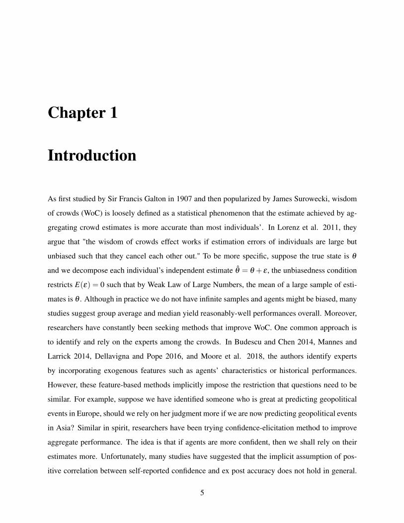
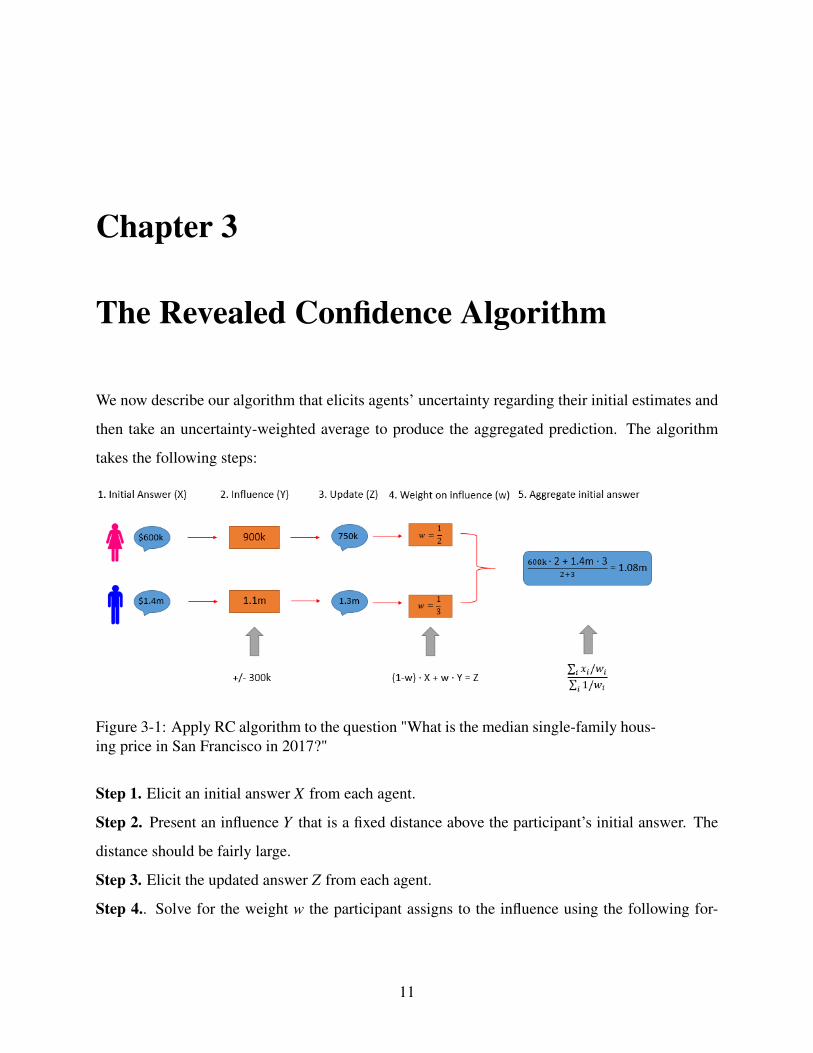
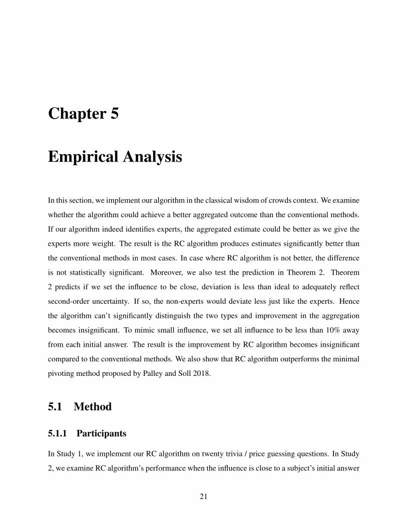
We now describe our algorithm that elicits agents’ uncertainty regarding their initial estimates and

then take an uncertainty-weighted average to produce the aggregated prediction. The algorithm

takes the following steps:

Figure 3-1: Apply RC algorithm to the question "What is the median single-family hous-ing price in San Francisco in 2017?"

Step 1. Elicit an initial answer X from each agent.

Step 2. Present an influence Y that is a fixed distance above the participant’s initial answer. The

distance should be fairly large.

Step 3. Elicit the updated answer Z from each agent.

Step 4.. Solve for the weight w the participant assigns to the influence using the following for-

11

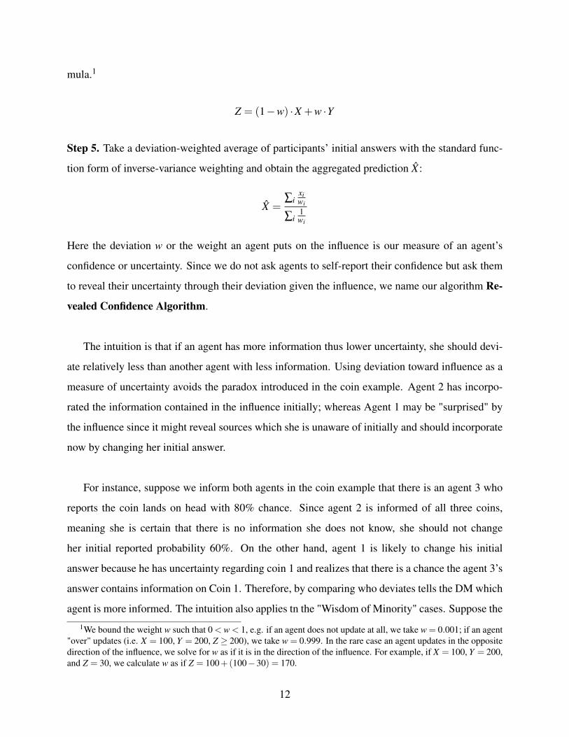
mula.1

Z = (1−w) ·X +w ·Y

Step 5. Take a deviation-weighted average of participants’ initial answers with the standard func-

tion form of inverse-variance weighting and obtain the aggregated prediction X :

X =∑i

xiwi

∑i1wi

Here the deviation w or the weight an agent puts on the influence is our measure of an agent’s

confidence or uncertainty. Since we do not ask agents to self-report their confidence but ask them

to reveal their uncertainty through their deviation given the influence, we name our algorithm Re-

vealed Confidence Algorithm.

The intuition is that if an agent has more information thus lower uncertainty, she should devi-

ate relatively less than another agent with less information. Using deviation toward influence as a

measure of uncertainty avoids the paradox introduced in the coin example. Agent 2 has incorpo-

rated the information contained in the influence initially; whereas Agent 1 may be "surprised" by

the influence since it might reveal sources which she is unaware of initially and should incorporate

now by changing her initial answer.

For instance, suppose we inform both agents in the coin example that there is an agent 3 who

reports the coin lands on head with 80% chance. Since agent 2 is informed of all three coins,

meaning she is certain that there is no information she does not know, she should not change

her initial reported probability 60%. On the other hand, agent 1 is likely to change his initial

answer because he has uncertainty regarding coin 1 and realizes that there is a chance the agent 3’s

answer contains information on Coin 1. Therefore, by comparing who deviates tells the DM which

agent is more informed. The intuition also applies tn the "Wisdom of Minority" cases. Suppose the

1We bound the weight w such that 0 < w < 1, e.g. if an agent does not update at all, we take w = 0.001; if an agent"over" updates (i.e. X = 100, Y = 200, Z ≥ 200), we take w = 0.999. In the rare case an agent updates in the oppositedirection of the influence, we solve for w as if it is in the direction of the influence. For example, if X = 100, Y = 200,and Z = 30, we calculate w as if Z = 100+(100−30) = 170.

12

question is "Is Philadelphia the state capitol of Pennsylvania?", many people would confidently say

"Yes" because they have the information that Philly is a large and famous city. However, what’s

unknown to them is that "the largest city in a state tends not to be the state capitol." When they

see an influence that the majority thinks the answer is "No", they are more likely to reflect on their

information (e.g. "Wow! So many people disagree with me. I must have missed some important

information.") and lower their reported confidence than those who really know the answer. In the

next sections, we theoretically analyze an agent’s updating mechanism and describes several key

properties of our algorithm.

13

Chapter 4

Updating Mechanism

Agents are asked to estimate an unknown quantity θ , which is the outcome of a random event.

Each agent i’s prior belief of θ is summarized as θ ∼ N(θi,τ2i ).

When she sees an influence influence y, which is the average of some other agents’ answers, she

also characterizes y∼N(θ ,σ2i ). We assume the prior variances follow inverse-gamma distribution

and all agents have a common prior for the variance of the influence: τ2i ∼ IG(ai,bi) and σ2

i ∼

IG(c,d).1 For notational simplicity, we omit the parameter for the number of agents by avoiding

expanding y into 1n ∑

nj=1 y j. The variances τ2

i and σ2i capture her first-order uncertainty. According

to Karni 2018, the agent may "entertain second-order belief regarding the likelihoods that different

first-order beliefs, are realized."2 It is natural to capture the second-order uncertainty by modeling

prior variance as a distribution instead of a constant3. Instead of having a full Bayesian MAP where

agents simultaneously update θ ,τ2i ,σ

2i , we assume the agents separately update these parameters to

capture an important empirical pattern, named the Distance Effect, which we will describe in detail

later. More specifically, given the influence, the agent first updates her prior variances, then she

plugs-in the first-order approximation of the posterior variances to the standard "fixed variances,

unknown mean" Bayesian updating function form, which aims at reducing her uncertainty of θ and

minimizing the expected quadratic loss. The updating of the prior variances follows the standard

1The mean and variance of IG(α,β ) is given by E(X) = β

α−1 and Var(X) = β 2

(α−1)2(α−2) .2Similar arguments are also manifested in Bewley 2002 which extends Savage (1954) and Anscombe and Aumann

(1963)’s framework to distinguish uncertainty from risk.3If a DM were to elicit an agent’s "confidence", we assume the agent reports the expectation of the inverse-gamma

distribution, which is the first-order uncertainty. The second-order uncertainty is the variance of the inverse-gammadistribution.

14

"Gaussian fixed mean, unknown variances" Bayesian updating scheme:

τ2i |y ∝ p(y|τ2

i )p(τ2i ) =⇒ τ

2i,post ∼ IG

(ai +

12,bi +

12(y− θi)

)(4.1)

σ2i |θi ∝ p(θi|σ2

i )p(σ2i ) =⇒ σ

2i,post ∼ IG

(c+

12,d +

12(y− θi)

)(4.2)

The first-order approximation is the expectation of τ2i,post and σ2

i,post . Now with the fixed posterior

variances, agents update θ and yields

E(θ |y) = θi +(y− θi)E(τ2

i,post)

E(τ2i,post)+E(σ2

i,post)= θi +∆iwi (4.3)

where

wi =

bi+12 (y−θi)

ai− 12

bi+12 (y−θi)

ai− 12

+d+ 1

2 (y−θi)

c− 12

(4.4)

We could interpret the updated estimate of θposti as the initial estimate θi adjusted toward y with

weights proportional to the ratio of the variances.

4.1 Identification of Relative Expertise & the Distance Effect

A crucial point is that agents’ uncertainty, which is measured by the hyperparameters in the inverse-

gamma distribution, is revealed in the weight assigned to the influence:

E(τ2A,post)

E(σ2A,post)

<E(τ2

B,post)

E(σ2A,post)

=⇒ E(τ2A,post)< E(τ2

B,post) =⇒ E(wA)< E(wB) (4.5)

Therefore, to make Equation 4.5 hold, it is absolutely important that we exogenously provide an

influence such that σ2A = σ2

B. Otherwise, the weight wi is not reflecting the prior uncertainty rather

some irrelevant factors induced by the researchers. For instance,suppose there are two agents

with the same information hence same level of uncertainty, we expect them to assign the same

15

weight to the influence. However, if the researcher gives one of them a more precise influence than

the other, the agent receiving the precise influence would deviate more, violating our identifying

mechanism. One probably counter-intuitive aspect is that y has to be different depending on each

agent’s initial estimate in order to control for the distance effect! We should observe in Equation

4.4 that weight wi depends on y− θi the distance between the initial estimate and the influence,

which is a parameter unrelated to uncertainty. This phenomenon is widely documented in many

empirical studies and also known as the distance effect, which refers to the within-person effect that

people tend to assign more weight to similar estimates than distant estimates (Yaniv 2004, Schultze

et al. 2015, Ravazzolo and Roisland 2011). Since we want the observed weight to be an indicator

only of prior variance, we should eliminate this confounder by setting the distance between the

initial estimate and the influence the same for everyone. Another important point is that we do not

want extreme distance. If ∆i is too large, bi becomes trivial. If ∆i is too small, ai becomes not as

significant. Nevertheless, we want the weight wi to be informative of both hyperparameters ai and

bi. We provide the full comparative statics analysis with respect to distance ∆ in Appendix 8.4.

A few other obvious aspects that affect σ2i , e.g.,the wording and the number of estimates we

take average from, are very easy to hold constant for every participant.

4.2 Second-order Uncertainty

We now look at how second-order uncertainty affects the algorithm. We know that the weight de-

pends on the posterior variance τ2i,post , which is determined by the hyperparameters of the inverse-

gamma distribution. Under the common prior assumption, the prior belief of others’ variance

σ2 ∼ IG(c,d) is the same across agents. Omitting subscript i, E(w) reduces to

w =

b+ 12 ∆

a− 12

b+ 12 ∆

a− 12+C

(4.6)

where C is some constant.

Hyperparameter a and b respectively dictates the variance and the mean of inverse-gamma

distribution. We could interpret b and a as proxies for first-order and second-order uncertainty,

16

respectively4. For instance, a small b and a large a imply low first-order and second-order uncer-

tainty. The "overconfident" agent introduced in the previous coin example corresponds to a small

b with small a, which implies a low first-order uncertainty but high second-order uncertainty5.

To give an example in the continuous setting, the question is "What is the median single family

housing price in San Francisco?" An agent who knows the median housing price of New York City

could have a relatively small b because NYC and SF are comparable; however, she has a small a

due to her ignorance of the housing market in the bay area. Although such agent could report a

small E(τ2), or low first-order uncertainty, the influence could potentially let her realize there ex-

ists new information she initially has not thought of and deviate more than what her expected prior

variance would suggest. Similarly, this could also explain why people with a high prior variance

are not deviating too much as one normally expects, e.g. they know they have full information and

understand the problem is very complex, so the influence is not providing them extra information

to better solve the problem .

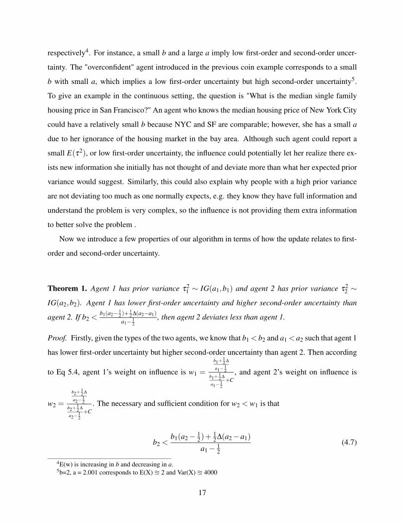
Now we introduce a few properties of our algorithm in terms of how the update relates to first-

order and second-order uncertainty.

Theorem 1. Agent 1 has prior variance τ21 ∼ IG(a1,b1) and agent 2 has prior variance τ2

2 ∼

IG(a2,b2). Agent 1 has lower first-order uncertainty and higher second-order uncertainty than

agent 2. If b2 <b1(a2− 1

2 )+12 ∆(a2−a1)

a1− 12

, then agent 2 deviates less than agent 1.

Proof. Firstly, given the types of the two agents, we know that b1 < b2 and a1 < a2 such that agent 1

has lower first-order uncertainty but higher second-order uncertainty than agent 2. Then according

to Eq 5.4, agent 1’s weight on influence is w1 =

b1+12 ∆

a1−12

b1+12 ∆

a1−12+C

, and agent 2’s weight on influence is

w2 =

b2+12 ∆

a2−12

b2+12 ∆

a2−12+C

. The necessary and sufficient condition for w2 < w1 is that

b2 <b1(a2− 1

2)+12∆(a2−a1)

a1− 12

(4.7)

4E(w) is increasing in b and decreasing in a.5b=2, a = 2.001 corresponds to E(X) u 2 and Var(X) u 4000

17

Theorem 1 characterizes how first-order and second-order uncertainty affect updating. As ar-

gued previously, a DM generally prefers an agent who can accurately assess his first-order uncer-

tainty than one who claims a low first-order uncertainty but indeed has no idea about the claim.

The condition stated in Theorem 1 shows that the RC algorithm, though not always, heavily favors

agent who has low second-order uncertainty. In Equation 4.7, b2 is the parameter which mainly

determines agent 2’s first-order variance. We can see that a2−a1a1− 1

2is scaled by the distance ∆. It al-

lows the first-order uncertainty to be "very high" before she deviates more than a low prior variance

and high second-order variance agent. For instance, let’s compare agent 1 with τ21 ∼ IG(1.5,1) and

agent 2 with τ22 ∼ IG(2.5,b2) and the distance ∆ between influence and the initial estimate is 10. b2

can be as large as 7 before agent 2 deviates more than agent 1. This corresponds to agent 2 having a

first-order uncertainty twice larger than agent 1’s before the algorithm can’t identify agent 2 as the

expert. This suggests that those who deviate less are fundamentally due to a small variance of their

prior variance. This is intuitive. Those who can precisely assess their prior variance should have

considered a large amount of information, which probably has already contained the information

conveyed by the influence. Therefore, the influence is less valuable to them relative to those who

do not have much information and hence can’t precisely estimate their prior variance.

Lemma 1. Given the same first-order prior variance, agents with low second-order variance

would assign strictly less weight to the influence than agents with high second-order variance.

Proof. See Appendix 8.2

Lemma 1 indicates our algorithm could solve a paradox traditional methods can’t. If two agents

reported the same variance or "confidence", traditional methods assume they are equally compe-

tent. However, as shown in our coin example, this might not be true. The RC algorithm could

identify the agent who is more certain of the reported confidence through their deviations.

It is obvious in our algorithm that more uncertainty should lead to more deviation given the

influence. More importantly, we should choose an influence that induces the revelation of second-

order uncertainty in addition to first-order uncertainty. The important distinction between the two

18

uncertainties is whether an agent views the prior variance as a constant or as a distribution. In the

former scenario, she does not update her variance. In the latter, she should update her variance

as suggested by Equation 5.4. We want the latter deviation to be larger than former because extra

uncertainty should be accompanied by extra deviation. Just to illustrate the idea with the previous

San Francisco housing price example, the agent who knows New York City’s housing price gives

an estimate of $800K. He is aware that he does not know the bay area housing market. But suppose

we give him an influence of $801K, he would think maybe the bay area housing price happened

to be similar to NYC’s. Therefore, he is probably more confident than he initially is and assigns

a small weight to the influence. The critical problem is the agent has a large second-order uncer-

tainty, his deviation does not properly reflect it because our influence lets him think he guessed the

bay area housing market correctly. However, if the influence is $2M, he would realize maybe the

bay area housing market is very different than what he assumed and then assigns a larger weight

to the influence to account for the previously unknown information. The next theorem provides

the cutoff point for the influence to properly reflect second-order information in addition to the first.

Theorem 2. An agent has prior variance τ2 ∼ IG(a,b) and assuming second-order uncertainty

exists. We need an influence such that ∆ > E(IG(a,b)) in order for the deviation to be larger than

if he has not considered second-order uncertainty.

Proof. See Appendix 8.3.

Theorem 2 shows that the influence should be reasonably far away from each agent’s initial

estimate. Otherwise, even though the agent has large second-order uncertainty and has the potential

to deviate a lot in a counter-factual world, they do not because the influence is too close. The

intuition is that a very close influence makes the agent think that there really is not much extra

information remaining or his initially unknown information happened to be close to his prior.

Overall, these three properties of our algorithm are truly advantageous when comparing our

method with other truth-telling mechanism that elicits a point estimate of confidence alone. If

the question is simple and there is not much second-order variance, RC algorithm works (at least

does not hurt) as it still reveals each agent’s confidence through their deviation. If the question

is complex such that people could be "confidently wrong" due to their incomplete information

19

, RC algorithm could potentially let participants realize that their confidence actually have large

uncertainty by showing them the influence. In this case, deviation reflects both first- and second-

order uncertainty, which improves identification of experts.

20

Chapter 5

Empirical Analysis

In this section, we implement our algorithm in the classical wisdom of crowds context. We examine

whether the algorithm could achieve a better aggregated outcome than the conventional methods.

If our algorithm indeed identifies experts, the aggregated estimate could be better as we give the

experts more weight. The result is the RC algorithm produces estimates significantly better than

the conventional methods in most cases. In case where RC algorithm is not better, the difference

is not statistically significant. Moreover, we also test the prediction in Theorem 2. Theorem

2 predicts if we set the influence to be close, deviation is less than ideal to adequately reflect

second-order uncertainty. If so, the non-experts would deviate less just like the experts. Hence

the algorithm can’t significantly distinguish the two types and improvement in the aggregation

becomes insignificant. To mimic small influence, we set all influence to be less than 10% away

from each initial answer. The result is the improvement by RC algorithm becomes insignificant

compared to the conventional methods. We also show that RC algorithm outperforms the minimal

pivoting method proposed by Palley and Soll 2018.

5.1 Method

5.1.1 Participants

In Study 1, we implement our RC algorithm on twenty trivia / price guessing questions. In Study

2, we examine RC algorithm’s performance when the influence is close to a subject’s initial answer

21

and compare with the results from Study 1. In Study 3, we compare the performance of RC algo-

rithm with the pivoting method proposed by Palley and Soll 2018. In Study 4, we implement RC

algorithms on ten stock price prediction questions. We recruit subjects from Amazon Mechanical

Turk (MTurk). For each study, we recruit 60 subjects who pass our very simple attention checks.

Following the recommendations of Berinsky, Margolis, and Sances (2014) we added two screener

questions that put a subtle instruction in the middle of a block of text. For example, in a block of

text ostensibly about people’s judgment of their performance, we ask participants to input specific

number (“33”) if they were reading the text. Another question is to ask immediately recall the

information provided in a previous page. The two attention checks both serve to examine whether

participants read the questions carefully. The passing rate for attention check is about 80%. Yet in

the data analysis, we do not exclude any participants1.

However, we do remove subjects whose score is in the bottom 10 percentile in the sample. The

purpose is to screen out insincere responses to the questions (e.g. those who enter "2" or "5" as an

answer to every question.). These insensible answers typically make the simple average perform

very poorly. We do not want our algorithms to improve upon an answer that barely has any value.

Overall, to those who may concern, our main results generally hold when including these subjects.

In reality, suppose a company manager is implementing our algorithm on her employees, she does

not need to exclude any subjects as we expect all responses are sincere.

5.1.2 Influence Selection

Participants provide their initial answer to a question before seeing an influence and providing

an updated answer. The influence is set to be a fixed percentage distance away from each initial

answer, e.g. |asnwer1±δ%|. Here are the guidelines for influence selection of a question.

1. The influence should be sensible. For example, we can’t provide a negative price as influence

or a price that is outrageously improbable.

2. The percentage distance varies across questions to avoid participants becoming suspicious.

1Excluding those subjects does not significantly change the main results.

22

3. The influence is at least 15% away from an initial answer.

4. The larger the coefficient of variation2 of an initial answer distribution, the larger percentage

distance.

5. If the kurtosis of the initial distribution is negative and the skewness is positive, meaning

there are many small answers but large answers are also present, we set the influence to be

above each initial answer.

6. If the kurtosis are very large (e.g. > 20), we set the influence to be above each initial answer.

7. Otherwise, we set the influence to be in the direction of the mean of the initial answers.

The above guideline is an empirical manifestation of our theoretical results: (1) the percentage dis-

tance between each initial estimate and the influence is the same to rule out the distance effect; (2)

the distance is relatively large so that participants could reflect on the second-order information.

In other words, the influence potentially reflects some new information they initially are not aware

of; (3) the distance is not too large such that the influence becomes insensible. One thing we need

to clarify is keeping percentage instead of absolute distance the same across participants. In our

previous model, we suggest distance effect makes agent with the same prior distribution to view

the precision of the influence differently. The hazard for using fix absolute distance is that people

have different prior means and they might view distance in percentage terms rather than absolute

terms. 3 For example, suppose the two initial answers are 10 and 10000, and the influence is 110

and 9900. "10" might view "110" as ten times larger, which is very far away from the initial an-

swer. "10000" might view "9900" as one percent away, which is very close to the initial estimate.

Therefore, holding the percentage distance constant may better account for the distance effect.

5.1.3 RC Estimate

To calculate the RC estimate, the deviation per subject per question is measured as the weight

assigned to the influence. Denote X1 and X2 as the initial and the updated answer, Y as the influence,

2standard deviation divided by mean of a distribution3(Note: how do people view numerical distance can be a separate research.)

23

w as the weight assigned to the influence. The updating process is captured by

(1−w)X1 +wY = X2

We could easily solve for w and take each w as the proxy for a participant’s prior variance of that

question. In the case where w = 0 or w ≥ 1, we set w = 0.001 and 0.999 respectively. In the rare

cases participants do not update in the direction of the influence, we calculate w as if the update is

in the direction of the influence. The RC algorithm forms the aggregated mean predictions using

the standard inverse-variance-weighted average over the initial answers, which has the property of

minimizing a prediction’s mean squared error. The formula is

RCavg =∑

Ni=1 X1i/wi

∑Ni=1 1/wi

Similarly for median, we take a variance-weighted median where the weight is 1/w.

5.2 Materials and Procedure

5.2.1 Tasks

Study 1 consists of twenty trivia and price guessing tasks. There are four questions in each task.

Firstly, a subject provides her initial answer to a question, e.g., "What is the median single-family

housing price of San Francisco in 2016?" Then we elicit a subject’s self-reported confidence over

the initial answer, which includes the belief of relative placement, which asks for whether the ac-

curacy of one’s initial answer is at the "bottom 20 percentile", "20th to 40th percentile", "40th to

60th percentile", "60th to 80th percentile", or the "top 20 percentile", as well as the probability

one’s initial answer is within 10% of the truth. Finally, we give the subject an influence and elicits

her updated answer.

In Study 2, we test our theoretical prediction of Theorem 2 using the same twenty tasks as in

Study 1. We examine whether a close influence (e.g. less than 10% away from an initial answer)

for each subject results in comparable improvement over group mean and median.

24

In Study 3, we use the same twenty questions as in Study 1 to compare the performance of RC

algorithm and the pivoting method. We elicit a subject’s initial answer along with her estimation

of the average answer of other subjects.

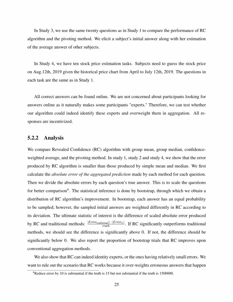
In Study 4, we have ten stock price estimation tasks. Subjects need to guess the stock price

on Aug.12th, 2019 given the historical price chart from April to July 12th, 2019. The questions in

each task are the same as in Study 1.

All correct answers can be found online. We are not concerned about participants looking for

answers online as it naturally makes some participants "experts." Therefore, we can test whether

our algorithm could indeed identify these experts and overweight them in aggregation. All re-

sponses are incentivized.

5.2.2 Analysis

We compare Revealed Confidence (RC) algorithm with group mean, group median, confidence-

weighted average, and the pivoting method. In study 1, study 2 and study 4, we show that the error

produced by RC algorithm is smaller than those produced by simple mean and median. We first

calculate the absolute error of the aggregated prediction made by each method for each question.

Then we divide the absolute errors by each question’s true answer. This is to scale the questions

for better comparison4. The statistical inference is done by bootstrap, through which we obtain a

distribution of RC algorithm’s improvement. In bootstrap, each answer has an equal probability

to be sampled; however, the sampled initial answers are weighted differently in RC according to

its deviation. The ultimate statistic of interest is the difference of scaled absolute error produced

by RC and traditional methods: |Errortraditional |−|Errorrc|truth . If RC significantly outperforms traditional

methods, we should see the difference is significantly above 0. If not, the difference should be

significantly below 0. We also report the proportion of bootstrap trials that RC improves upon

conventional aggregation methods.

We also show that RC can indeed identity experts, or the ones having relatively small errors. We

want to rule out the scenario that RC works because it over-weights erroneous answers that happen4Reduce error by 10 is substantial if the truth is 15 but not substantial if the truth is 1500000.

25

to cancel each other out. We first calculate the absolute error of each answer scaled by the truth.

Therefore, errors can’t cancel out when we aggregate them. Then we calculate the aggregated

absolute errors produced by each method. We employ the similar bootstrap procedure described

above as a basis of our statistical inference. In addition to the bootstrap, we also run a regression

of each answer’s percentage error on each answer’s respective weight on the influence (deviation)

with standard errors clustered on each question (Note: we remove outliers before running the

regression.). We expect the coefficient to be positive, meaning those who deviate more tend to

have larger absolute errors.

In Study 3, we compare RC algorithm and the minimal pivoting method (Palley and Soll 2018)

on their ability to improve upon conventional methods. Firstly, we examine in how many questions

RC has larger improvement on the group mean than pivoting. Then for each question, we use boot-

strap to obtain the distribution of the difference of improvement upon group of the two methods.

We describe the procedure of the minimal pivoting method in detail in the Discussion section.

The results of a non-parametric test on the difference of performance of different methods on

the question level are presented in Appendix B.

5.3 Results

5.3.1 Study 1: RC vs Conventional Methods

All results are plotted in Figure 5-1. Firstly, RC algorithm yields a better performance than group

mean in 15 out of 20 questions. Among the 15 improvements, 9 improvements are statistically

significant at 5% level. The 5 non-improvements are not statistically significant, meaning the

worse aggregated prediction made by RC algorithm can simply be explained by sampling variance.

Therefore, we say that applying RC algorithm may improve the aggregated prediction significantly

but it does not degrade the prediction. To understand why RC algorithm tends to dominate group

mean (simple average), we look at which answers RC algorithm tend to overweight in the aggre-

gation. As we can see in Figure 5.1, in 16 out of 20 questions, RC produces a significantly smaller

average absolute errors than group mean. In addition, a regression of each answer’s error on each

answer’s respective weight on influence confirms this result (β = 0.391, p.value < 0.001). Such

26

result indicates RC algorithm indeed could identity answers with smaller errors and give them

larger weight in aggregation. In the 4 questions which RC algorithm does not significantly over-

weight those answers with smaller errors, it does not select those with larger errors either. Such

result indicates that the initial answers in these four questions are fairly accurate in the first place.

Therefore, there is not much room for further improvement. Nevertheless, RC algorithm does not

degrade the initial answers by overweighting those with slightly larger errors either.

27

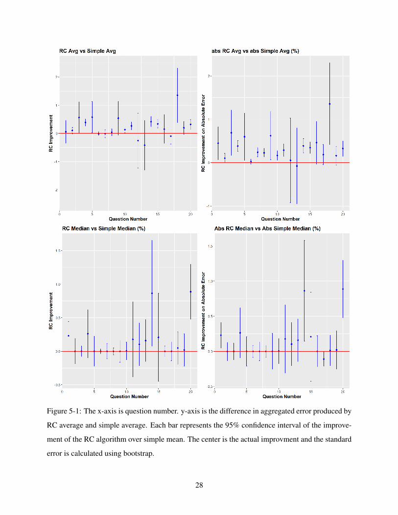
Figure 5-1: The x-axis is question number. y-axis is the difference in aggregated error produced by

RC average and simple average. Each bar represents the 95% confidence interval of the improve-

ment of the RC algorithm over simple mean. The center is the actual improvment and the standard

error is calculated using bootstrap.

28

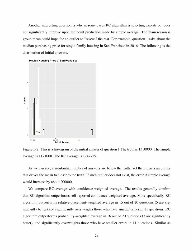
Another interesting question is why in some cases RC algorithm is selecting experts but does

not significantly improve upon the point prediction made by simple average. The main reason is

group mean could hope for an outlier to "rescue" the rest. For example, question 1 asks about the

median purchasing price for single family housing in San Francisco in 2016. The following is the

distribution of initial answers.

Figure 5-2: This is a histogram of the initial answer of question 1.The truth is 1310000. The simple

average is 1171000. The RC average is 1247755.

As we can see, a substantial number of answers are below the truth. Yet there exists an outlier

that drives the mean to closer to the truth. If such outlier does not exist, the error if simple average

would increase by about 200000.

We compare RC average with confidence-weighted average. The results generally confirm

that RC algorithm outperforms self-reported confidence weighted average. More specifically, RC

algorithm outperforms relative-placement-weighted average in 15 out of 20 questions (5 are sig-

nificantly better) and significantly overweights those who have smaller errors in 11 questions. RC

algorithm outperforms probability-weighted average in 16 out of 20 questions (3 are significantly

better), and significantly overweights those who have smaller errors in 11 questions. Similar as

29

before, RC does not perform significantly worse than confidence-weighted average.

Another common WoC approach is to take the group median (simple median). The RC algo-

rithm also adapts to median since we only need to take a inverse variance weighted median with

w being the weights. The result is comparable to that regarding simple average. RC median does

not perform worse than simple median in all twenty questions and 3 of them being significantly

better and 0 of them significantly worse. In this particular pilot, it seems group median is better

than group mean. Nevertheless, RC algorithm could improve upon either measure.

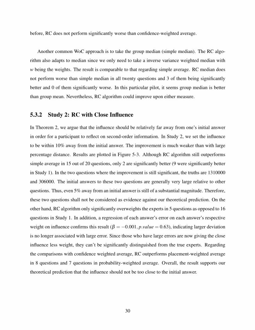
5.3.2 Study 2: RC with Close Influence

In Theorem 2, we argue that the influence should be relatively far away from one’s initial answer

in order for a participant to reflect on second-order information. In Study 2, we set the influence

to be within 10% away from the initial answer. The improvement is much weaker than with large

percentage distance. Results are plotted in Figure 5-3. Although RC algorithm still outperforms

simple average in 15 out of 20 questions, only 2 are significantly better (9 were significantly better

in Study 1). In the two questions where the improvement is still significant, the truths are 1310000

and 306000. The initial answers to these two questions are generally very large relative to other

questions. Thus, even 5% away from an initial answer is still of a substantial magnitude. Therefore,

these two questions shall not be considered as evidence against our theoretical prediction. On the

other hand, RC algorithm only significantly overweights the experts in 5 questions as opposed to 16

questions in Study 1. In addition, a regression of each answer’s error on each answer’s respective

weight on influence confirms this result (β =−0.001, p.value = 0.63), indicating larger deviation

is no longer associated with large error. Since those who have large errors are now giving the close

influence less weight, they can’t be significantly distinguished from the true experts. Regarding

the comparisons with confidence weighted average, RC outperforms placement-weighted average

in 8 questions and 7 questions in probability-weighted average. Overall, the result supports our

theoretical prediction that the influence should not be too close to the initial answer.

30

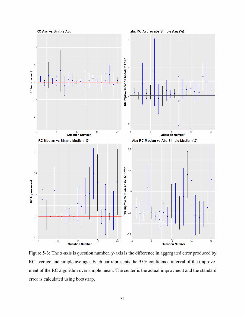
Figure 5-3: The x-axis is question number. y-axis is the difference in aggregated error produced by

RC average and simple average. Each bar represents the 95% confidence interval of the improve-

ment of the RC algorithm over simple mean. The center is the actual improvment and the standard

error is calculated using bootstrap.

31

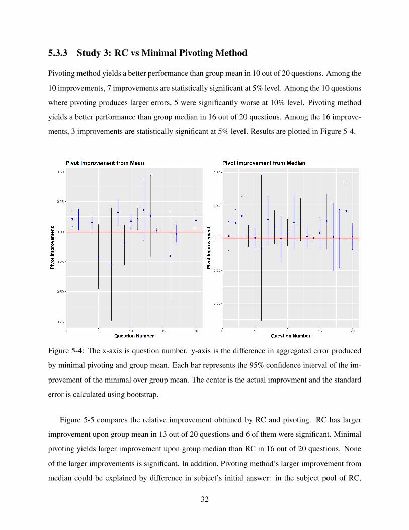
5.3.3 Study 3: RC vs Minimal Pivoting Method

Pivoting method yields a better performance than group mean in 10 out of 20 questions. Among the

10 improvements, 7 improvements are statistically significant at 5% level. Among the 10 questions

where pivoting produces larger errors, 5 were significantly worse at 10% level. Pivoting method

yields a better performance than group median in 16 out of 20 questions. Among the 16 improve-

ments, 3 improvements are statistically significant at 5% level. Results are plotted in Figure 5-4.

Figure 5-4: The x-axis is question number. y-axis is the difference in aggregated error produced

by minimal pivoting and group mean. Each bar represents the 95% confidence interval of the im-

provement of the minimal over group mean. The center is the actual improvment and the standard

error is calculated using bootstrap.

Figure 5-5 compares the relative improvement obtained by RC and pivoting. RC has larger

improvement upon group mean in 13 out of 20 questions and 6 of them were significant. Minimal

pivoting yields larger improvement upon group median than RC in 16 out of 20 questions. None

of the larger improvements is significant. In addition, Pivoting method’s larger improvement from

median could be explained by difference in subject’s initial answer: in the subject pool of RC,

32

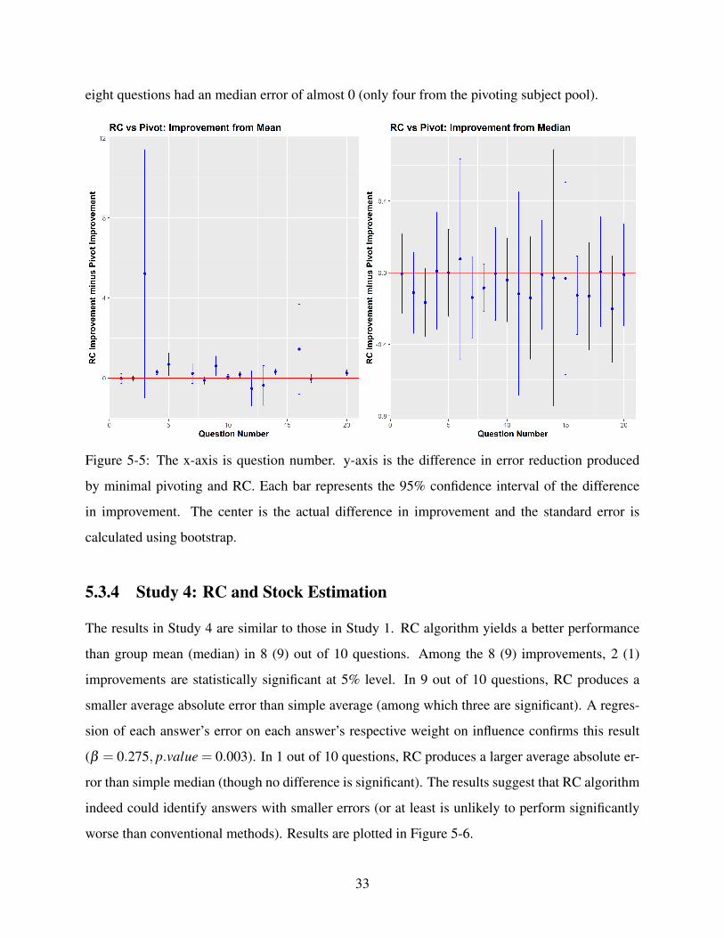
eight questions had an median error of almost 0 (only four from the pivoting subject pool).

Figure 5-5: The x-axis is question number. y-axis is the difference in error reduction produced

by minimal pivoting and RC. Each bar represents the 95% confidence interval of the difference

in improvement. The center is the actual difference in improvement and the standard error is

calculated using bootstrap.

5.3.4 Study 4: RC and Stock Estimation

The results in Study 4 are similar to those in Study 1. RC algorithm yields a better performance

than group mean (median) in 8 (9) out of 10 questions. Among the 8 (9) improvements, 2 (1)

improvements are statistically significant at 5% level. In 9 out of 10 questions, RC produces a

smaller average absolute error than simple average (among which three are significant). A regres-

sion of each answer’s error on each answer’s respective weight on influence confirms this result

(β = 0.275, p.value = 0.003). In 1 out of 10 questions, RC produces a larger average absolute er-

ror than simple median (though no difference is significant). The results suggest that RC algorithm

indeed could identify answers with smaller errors (or at least is unlikely to perform significantly

worse than conventional methods). Results are plotted in Figure 5-6.

33

34

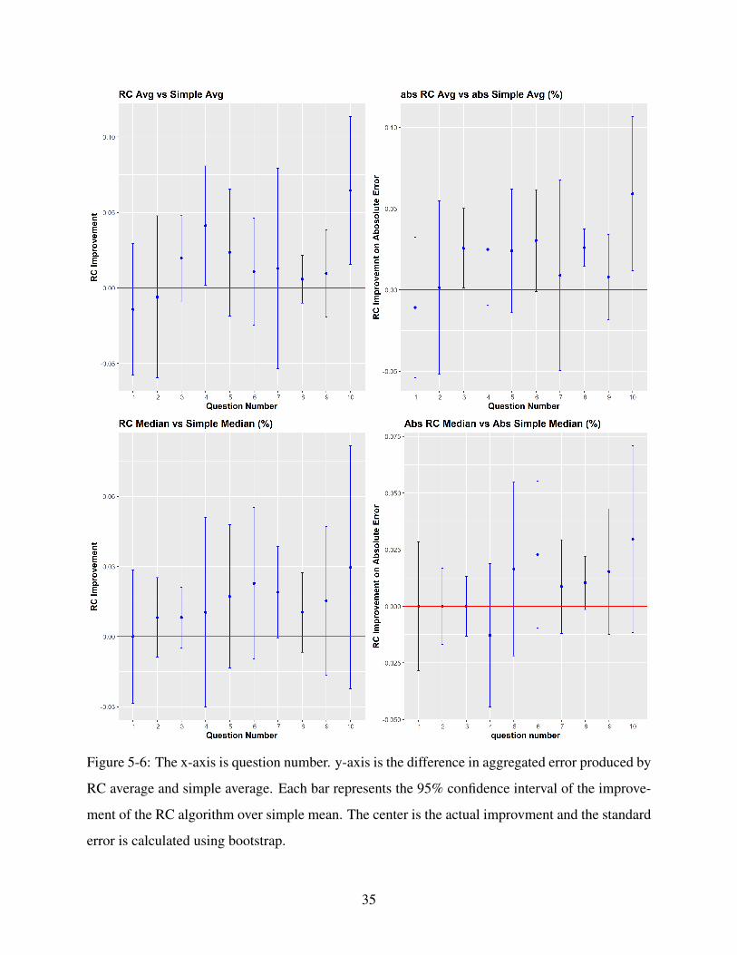
Figure 5-6: The x-axis is question number. y-axis is the difference in aggregated error produced by

RC average and simple average. Each bar represents the 95% confidence interval of the improve-

ment of the RC algorithm over simple mean. The center is the actual improvment and the standard

error is calculated using bootstrap.

35

Chapter 6

Discussion

6.1 When does the Algorithm work or does not work?

No single algorithm serves as a panacea to all WoC problems under all conditions. We feel it is

very important to point out the conditions that our algorithm works, since in the theoretical models

we tend to assume away the anomalies.

Firstly, we should acknowledge that the conventional wisdom of crowds methods are not bad.

In some cases, they indeed provide a great aggregated estimate. For example, Q6 asks for the

standard monthly subscription fee for Netflex in 2019. The truth is $12.99 and the group mean is

$12.98, which is very accurate. In this case, there is almost no room for RC algorithm to improve

upon. However, the important message is even in this case applying RC algorithm does not signif-

icantly degrade the aggregated estimate either1.

Secondly, we need experts in the crowds. Suppose the question is very difficult and no one

knows the answer, then we could imagine that everyone would give the influence a large weight

and the algorithm does not work because simply there does not even exist an expert to over-weight.

Nevertheless, the empirical results have shown that RC algorithms does not under-perform simple

average since the algorithm only weights the relative deviation: if everyone deviates a lot, say 90%,

it is as if no one deviates since everyone would receive an equal weight.

1The RC average is $12.01.

36

Thirdly, for the RC algorithm to work well and the aggregated prediction to have a small error,

we need participants not to be stubborn. Consider Figure 5.5, if that outlier happened to be "stub-

born" and does not deviate at all, the RC algorithm might perform less well. However, in reality, if

the incentive is sufficiently attractive, we expect people to account for information more rationally.

In Appendix ??, we provide a theoretical analysis on how different behavioral bias could poten-

tially affect the algorithm. Nevertheless, how to account for people’s different biases to further

improve RC algorithm is beyond the discussion of this paper.

6.2 Experts & Confidence

After noting the coin example in the beginning, we may want to examine how we should define

overconfidence and classify experts ex ante2. In many previous studies, researchers ex ante classify

experts as those who state a higher probability (confidence) and evaluate overconfidence simply

by comparing an agent’s subjective probability with the realized outcome. However, measuring

ex ante confidence by ex post accuracy can be problematic. As illustrated in the coin example,

a higher probability by no means implies better knowledge; an outcome against prediction does

not imply the prediction is not ex ante optimal3. In this paper, we propose using deviation under

influence as a measure for uncertainty. As shown in the appendix, this deviation satisfies the

criterion as a valid measure for uncertainty. Under our framework, we define experts as those

who deviate less because these people tend to have more informed of the event. Our framework

also provides a rational justification of over-confidence in terms of overprecision. Even though

agents are reporting their best point estimates for their prior variance, which is the expectation

of the distribution of their prior variance, they could still have much uncertainty in their reported

variance, which previous researchers often fail to account for in the first place.

2Ex post definition can be simply defined by the discrepancy between an answer and the truth. However, suchmeasure is not helpful in prediction contexts.

3ex ante optimality does not guarantee ex post correctness.

37

6.3 Surprisingly Popular Algorithm

Prelec et al. 2017 proposes the Surprisingly Popular (SP) algorithm, which also serves to improve

wisdom of crowds. SP algorithm elicits agents’ initial answers along with their predictions of

the proportion of their peers agreeing with their initial answers. Then the SP algorithm gives the

following formula in a binary question. Denote PA the actual proportion of agents choosing A;

EA the proportion of agents expected to choosing A; PB the actual proportion of agents choosing

B; EB the proportion of agents expected to choosing B. If PA−EA > PB−EB, then the algorithm

chooses choice A. If PA−EA < PB−EB, then the algorithm chooses choice B. The theoretical

intuition, as argued in Prelec et al. 2017, is that a Bayesian agent receiving a signal from the true

state tends to under-predict the proportion of peers that actually choose that answer. Although the

theoretical frameworks of RC algorithm and SP algorithm are different, the fact that an agent who

is willing to predict the option she did not choose is more popular indicates she is resistant to the

majority’s influence (wiling to be the minority)! Hence the SP algorithm overweights the opinion

of such agent in the aggregation. Nevertheless, although in theory the SP algorithm could extend to

questions with a continuous solution space, it is not hard to imagine that the cognitive load required

to accurately characterize the exact distribution of other agents’ answers, e.g. the medium housing

price of San Francisco, is non-trivial. On the other hand, RC only encourages agent to account for

the given influence to obtain a better outcome, which is simply more manageable.

6.4 The Minimal Pivoting Method

In our paper, we compare RC algorithm with the minimal pivoting method, which is an algorithm

fitted for a continuous question. In this section, we describe the procedures for the minimal pivoting

method and explain the basic intuition behind. The pivoting method (Palley and Soll 2018) is a peer

prediction method aiming at distinguishing agents’ private information from shared information.

Agents who have more private information as opposed to share information are considered the

experts. The method requires agents to provide both their own best judgment, say X , and an

estimate Y of the average judgment that will be given by all other agents. The minimal method

transforms each X into 2X−Y before aggregating (e.g., averaging) over the transformed estimates.

38

The intuition is that if an agent only has shared information, his estimate Y of other agents’ average

is more likely to be X , because he only knows what everyone else knows. So his transformed

estimate is 2X−X =X . On the other hand, if an agent has much private information, her estimate Y

of other agents is likely to be very different from X , or the common knowledge. So her transformed

estimate is 2X −Y = 2(Y + δ )−Y = Y + 2δ , where δ represents private information. And the

private information is weighted extra in the aggregation. The full pivoting method serves to adjust

the degree private information is overweighted, but it is fairly complicated to execute. That’s why

we only implement the minimal pivoting.

39

Chapter 7

Conclusion

In this paper, we propose our Revealed Confidence algorithm could improve Wisdom of Crowds.

The algorithm invites agents to reveal their confidence through their deviation under an influence

as opposed to the conventional self-reported confidence. The advantage of using deviation given

influence as a measure for uncertainty is it reflects both first-order and second-order uncertainty,

where conventional confidence elicitation only elicits the former. In our theoretical results, we

incorporate the distance effect into our belief-updating model and show that (1) deviation depends

more on the second-order uncertainty than first-order uncertainty (2) an influence too close to the

initial answer is insufficient to induce the revelation of second-order uncertainty. Our empirical

results verify the theoretical predictions (1) those who are more knowledgeable or accurate (or

those who have lower first-order and second-order uncertainty) tends to deviate less1 and get over-

weighted by the algorithm in the aggregation (2) a close influence would muddle the distinction

between the experts and non-experts because the non-experts deviate less relative to under a far

influence. In the discussion, we highlight the restrictions of our algorithm, which is also a direction

for future research. For example, suppose we could have a method to identify agents who are

simply too stubborn to be influenced, the performance of RC could be further improved.

1Put a smaller weight on the influence

40

Chapter 8

Appendix A: Theory Results

8.1 Coin Example and Blackwell’s Information Structure

The coin example aforementioned in the main text highlights the distinction between first- and

second-order uncertainty: the former is based on the currently known information, whereas the

latter is based on the currently unknown information. Here we explain how the concepts fits in

Blackwell’s information structure framework (Blackwell 1951, 1953). The key components in

Blackwell’s information structure are the states of nature and the signals. In statistical games,

"each state of nature constitute the pure strategies nature could select (Blackwell and Girshick

1954). In the coin example, nature is playing a sequential game: first, nature selects one of the

three coins; second, nature flips the selected coin. Let Ω = ω1, ...,ωK be a finite set of states.

Let S = s1, ...,sJ be a set of signals that an agent observes. An information structure Q is defined

as a Markov matrix with dimension K×J, where Qk j is the probability signal s j is observed given

a state ωk. In Blackwell 1951, DM acts based on the information structure (or the signals an agent

receives) and the DM’s utility depends on the action and the realized state. The Blackwell’s theo-

rem (Blackwell 1951) states that

"Q is more Blackwell informative than P if and only if there exists a Markov matrix M such

that QM = P."

The Blackwell theorem characterizes a condition where action according to a more "Blackwell

41

informative" information structure leads to a weakly better expected utility for any given decision

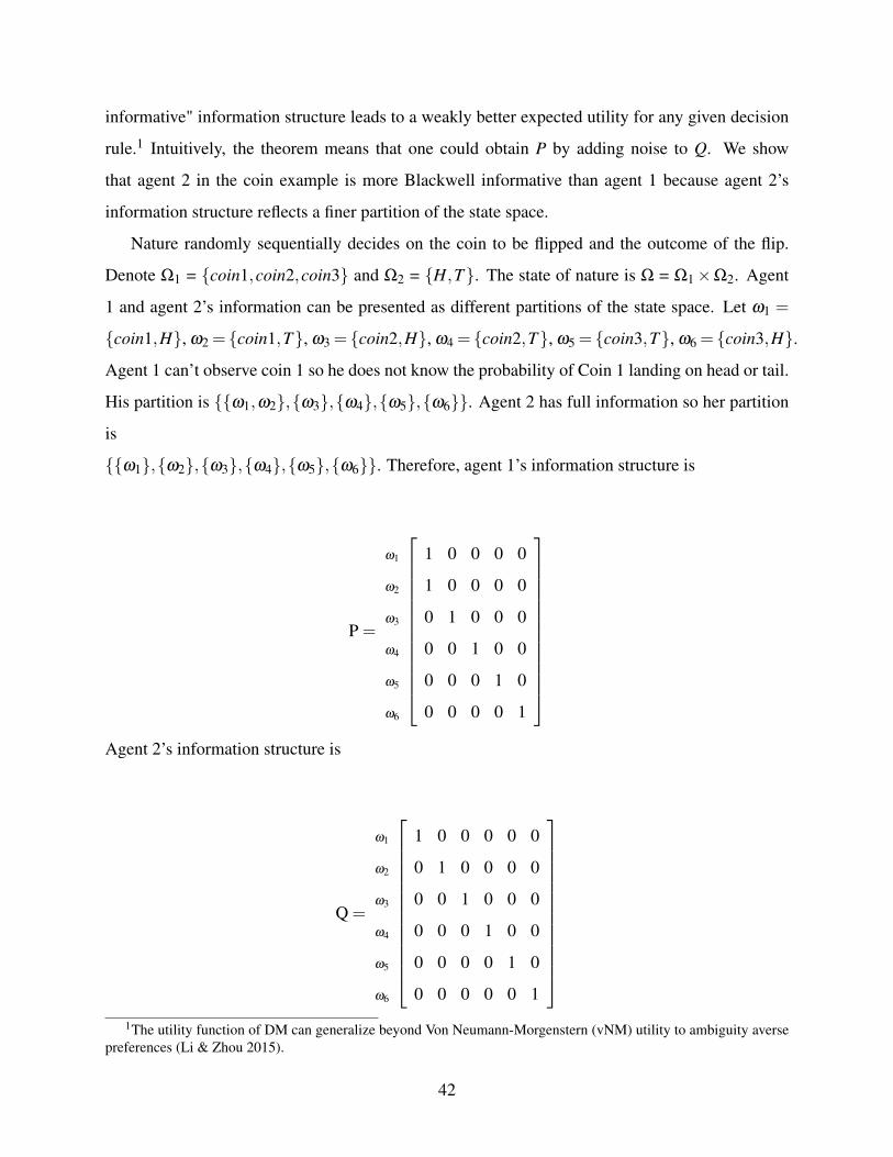
rule.1 Intuitively, the theorem means that one could obtain P by adding noise to Q. We show

that agent 2 in the coin example is more Blackwell informative than agent 1 because agent 2’s

information structure reflects a finer partition of the state space.

Nature randomly sequentially decides on the coin to be flipped and the outcome of the flip.

Denote Ω1 = coin1,coin2,coin3 and Ω2 = H,T. The state of nature is Ω = Ω1×Ω2. Agent

1 and agent 2’s information can be presented as different partitions of the state space. Let ω1 =

coin1,H, ω2 = coin1,T, ω3 = coin2,H, ω4 = coin2,T, ω5 = coin3,T, ω6 = coin3,H.

Agent 1 can’t observe coin 1 so he does not know the probability of Coin 1 landing on head or tail.

His partition is ω1,ω2,ω3,ω4,ω5,ω6. Agent 2 has full information so her partition

is

ω1,ω2,ω3,ω4,ω5,ω6. Therefore, agent 1’s information structure is

P =

ω1 1 0 0 0 0

ω2 1 0 0 0 0

ω3 0 1 0 0 0

ω4 0 0 1 0 0

ω5 0 0 0 1 0

ω6 0 0 0 0 1

Agent 2’s information structure is

Q =

ω1 1 0 0 0 0 0

ω2 0 1 0 0 0 0

ω3 0 0 1 0 0 0

ω4 0 0 0 1 0 0

ω5 0 0 0 0 1 0

ω6 0 0 0 0 0 1

1The utility function of DM can generalize beyond Von Neumann-Morgenstern (vNM) utility to ambiguity averse

preferences (Li & Zhou 2015).

42

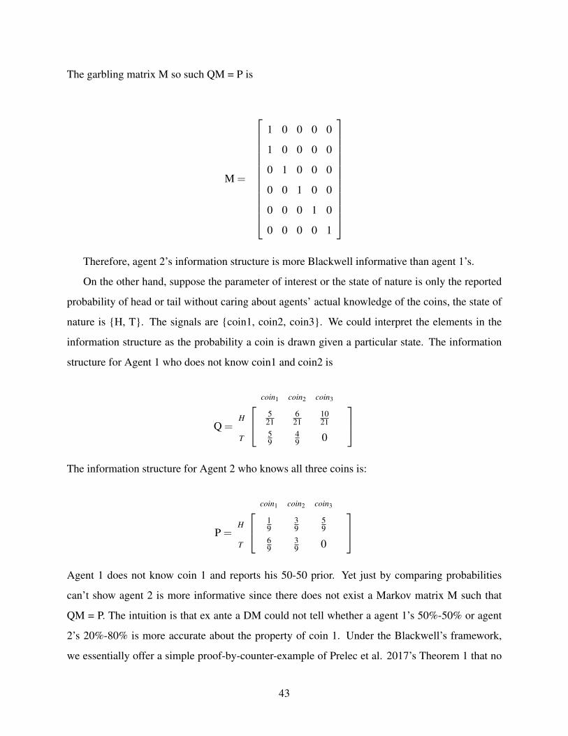
The garbling matrix M so such QM = P is

M =

1 0 0 0 0

1 0 0 0 0

0 1 0 0 0

0 0 1 0 0

0 0 0 1 0

0 0 0 0 1

Therefore, agent 2’s information structure is more Blackwell informative than agent 1’s.

On the other hand, suppose the parameter of interest or the state of nature is only the reported

probability of head or tail without caring about agents’ actual knowledge of the coins, the state of

nature is H, T. The signals are coin1, coin2, coin3. We could interpret the elements in the

information structure as the probability a coin is drawn given a particular state. The information

structure for Agent 1 who does not know coin1 and coin2 is

Q =

coin1 coin2 coin3

H 521

621

1021

T 59

49 0

The information structure for Agent 2 who knows all three coins is:

P =

coin1 coin2 coin3

H 19

39

59

T 69

39 0

Agent 1 does not know coin 1 and reports his 50-50 prior. Yet just by comparing probabilities

can’t show agent 2 is more informative since there does not exist a Markov matrix M such that

QM = P. The intuition is that ex ante a DM could not tell whether a agent 1’s 50%-50% or agent

2’s 20%-80% is more accurate about the property of coin 1. Under the Blackwell’s framework,

we essentially offer a simple proof-by-counter-example of Prelec et al. 2017’s Theorem 1 that no

43

algorithm based on first-order information is guaranteed to deduce the correct answer.

8.2 Proof of Lemma 1

Suppose agent 1 has reported prior variance τ2 = E(IG(a1,b1)) =b1

a1−1 , according to Eq 5.4, agent

1’s weight on influence is w1 =

b1+12 ∆

a1−12

b1+12 ∆

a1−12+C

. Agent 2’s distribution of prior variance is IG(a2,b2) such

that

b2

a2−1=

b1

a1−1(8.1)

b22

(a2−1)2(a2−2)<

b21

(a1−1)2(a1−2)(8.2)

Wlog, we take a2 = a1 + ε and b2 =b1(a1+ε−1)

a1−1 where ε > 0. As shown in Theorem 1, in order for

w2 < w1, we need

b2 =b1(a1 + ε−1)

a1−1<

b1(a2− 12)+

12∆(a2−a1)

a1− 12

(8.3)

(a1 + ε−1)<(a1−1)(a2− 1

2)

a1− 12

+κ (8.4)

ε < (a1−1)(a2− 1

2

a1− 12

−1)+12(a1−1)∆ε

a1− 12

(8.5)

We can arbitrarily set ∆ > 2a1−1a1−1 so the above condition always holds.

8.3 Proof of Theorem 2

proof:

If an agent considers only first-order uncertainty without second-order uncertainty, it means she

treats the variance as a constant and does not update her prior variance given the influence. The

44

weight assigned to influence as given by Equation 5.1 is w1, f irst =b

a−1b

a−1+C, in which the agent di-

rectly takes the expectation of τ2 without updating. In other words, this is the weight if the agent

simply "neglects" she has uncertainty regarding her assessment of variance. If she updates her

prior variance, the weight assigned to influence as given by Equation 5.3 is w1 =

b+ 12 ∆

a− 12

b+ 12 ∆

a− 12+C

. As we

want to observe agent 1 assigning more weight to the influence if she were to account for the extra

uncertainty, we need w1 > w1, f irst , and the necessary and sufficient condition for w1−w1, f irst > 0

is ∆ > ba−1 = E(IG(a,b)).

For example, consider IG(3, 10) as the distribution for τ2 and assume C = 10. The expectation

E(τ2) is 5, which is her first order variance. The weight assigned to influence without considering

second-order variance (treating the variance simply as 5 instead of IG(3,10)) is w1, f irst =13 . Let

∆ = 2 < E(IG(3,10)). If the agent considers second-order information and updates the prior

variance, her weight is w1 u 30.5% < 13 , given by Equation 5.3. Let ∆ = 10 > E(IG(3,10)). The

weight w1 is 37.5%. Therefore, if ∆ < 5, the w1 is not reflecting the extra second-order uncertainty

as it could with ∆ > 5.

8.4 Distance Effect: Comparative Statics

We take derivative of w with respect to ∆. For Visual representation of the distance effect, please

see Figure 9.1-9.4

∂wd∆

=0.5(2a−1)(2c−1)(d−b)(

a(2d +∆)+b(2c−1)+(c−1)∆−d)2

where ∆ = y− θ

d−b > 0 =⇒ ∂wd∆

> 0

d−b < 0 =⇒ ∂wd∆

< 0

45

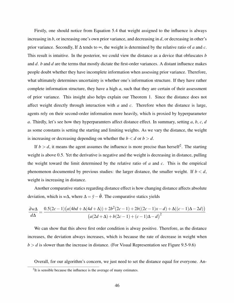
Firstly, one should notice from Equation 5.4 that weight assigned to the influence is always

increasing in b, or increasing one’s own prior variance, and decreasing in d, or decreasing in other’s

prior variance. Secondly, If ∆ tends to ∞, the weight is determined by the relative ratio of a and c.

This result is intuitive. In the posterior, we could view the distance as a device that obfuscates b

and d. b and d are the terms that mostly dictate the first-order variances. A distant influence makes

people doubt whether they have incomplete information when assessing prior variance. Therefore,

what ultimately determines uncertainty is whether one’s information structure. If they have rather

complete information structure, they have a high a, such that they are certain of their assessment

of prior variance. This insight also helps explain our Theorem 1. Since the distance does not

affect weight directly through interaction with a and c. Therefore when the distance is large,

agents rely on their second-order information more heavily, which is proxied by hyperparameter

a. Thirdly, let’s see how they hyperparamters affect distance effect. In summary, setting a, b, c, d

as some constants is setting the starting and limiting weights. As we vary the distance, the weight

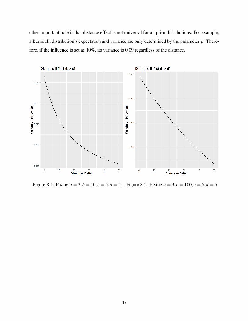
is increasing or decreasing depending on whether the b < d or b > d.

If b > d, it means the agent assumes the influence is more precise than herself2. The starting

weight is above 0.5. Yet the derivative is negative and the weight is decreasing in distance, pulling

the weight toward the limit determined by the relative ratio of a and c. This is the empirical

phenomenon documented by previous studies: the larger distance, the smaller weight. If b < d,

weight is increasing in distance.

Another comparative statics regarding distance effect is how changing distance affects absolute

deviation, which is w∆, where ∆ = y− θ . The comparative statics yields

∂w∆

d∆=

0.5(2c−1)(a(4bd +∆(4d +∆))+2b2(2c−1)+2b((2c−1)x−d)+∆((c−1)∆−2d)

)(a(2d +∆)+b(2c−1)+(c−1)∆−d

)2

We can show that this above first order condition is alway positive. Therefore, as the distance

increases, the deviation always increases, which is because the rate of decrease in weight when

b > d is slower than the increase in distance. (For Visual Representation see Figure 9.5-9.6)

Overall, for our algorithm’s concern, we just need to set the distance equal for everyone. An-

2It is sensible because the influence is the average of many estimates.

46

other important note is that distance effect is not universal for all prior distributions. For example,

a Bernoulli distribution’s expectation and variance are only determined by the parameter p. There-

fore, if the influence is set as 10%, its variance is 0.09 regardless of the distance.

Figure 8-1: Fixing a = 3,b = 10,c = 5,d = 5 Figure 8-2: Fixing a = 3,b = 100,c = 5,d = 5

47

Figure 8-3: Fixing a = 3,b = 5,c = 5,d = 10 Figure 8-4: Fixing a = 3,b = 5,c = 5,d = 100

Figure 8-5: Fixing a = 3,b = 30,c = 3,d = 3. Figure 8-6: Fixing a = 3,b = 3,c = 30,d = 3

48

Chapter 9

Appendix B: Empirical Results

Question Mean Error RC Mean Error P-value Median Error RC Median Error P-value1 -0.11 -0.05 0.12 -0.24 -0.01 0.002 -0.22 -0.12 0.03 0.00 0.00 0.083 0.60 0.03 0.00 0.00 0.00 0.004 -0.43 -0.04 0.00 -0.28 -0.02 0.005 0.83 0.25 0.00 0.00 0.00 0.016 -0.07 -0.08 0.69 0.00 0.00 0.017 -0.04 -0.05 0.42 0.00 0.00 0.018 -0.06 0.02 0.31 0.00 0.00 0.409 0.75 0.21 0.01 0.01 0.01 0.00

10 -0.20 -0.06 0.00 -0.00 0.00 0.0411 -0.38 -0.11 0.00 -0.18 0.00 0.0512 0.20 0.46 0.74 -0.10 0.00 0.0513 -0.12 0.53 0.64 -0.16 0.00 0.0014 -0.51 -0.10 0.00 -0.89 0.03 0.2215 -0.42 -0.08 0.00 -0.21 -0.01 0.0016 0.16 -0.01 0.15 0.00 0.00 0.0017 0.04 0.13 0.65 0.12 0.12 0.4718 1.38 0.02 0.00 0.05 0.00 0.0019 -0.23 0.03 0.14 -0.02 -0.00 0.0020 -0.57 -0.25 0.00 -0.89 0.00 0.00

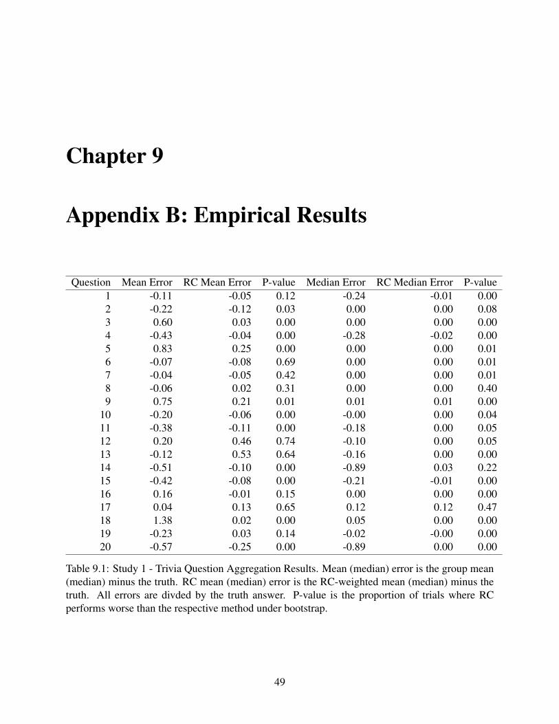
Table 9.1: Study 1 - Trivia Question Aggregation Results. Mean (median) error is the group mean(median) minus the truth. RC mean (median) error is the RC-weighted mean (median) minus thetruth. All errors are divded by the truth answer. P-value is the proportion of trials where RCperforms worse than the respective method under bootstrap.

49

Question Mean Error RC Mean Error P-value Median Error RC Median Error P-value1 -0.36 -0.17 0.00 -0.39 -0.01 0.002 -0.25 -0.30 0.91 -0.07 -0.03 0.363 0.61 0.20 0.11 0.00 0.00 0.004 -0.51 -0.44 0.08 -0.74 -0.14 0.095 0.27 0.19 0.27 0.00 0.00 0.006 0.75 -0.09 0.14 0.00 0.00 0.157 0.08 0.29 0.82 -0.01 0.00 0.018 -0.15 -0.01 0.29 -0.01 0.00 0.329 0.44 0.36 0.30 0.01 0.01 0.16

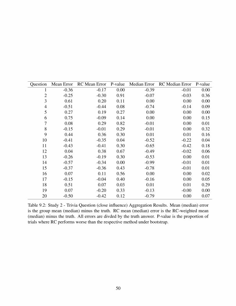
10 -0.41 -0.35 0.04 -0.52 -0.22 0.0411 -0.43 -0.41 0.30 -0.65 -0.42 0.1812 0.04 0.38 0.67 -0.49 -0.02 0.0613 -0.26 -0.19 0.30 -0.53 0.00 0.0114 -0.57 -0.34 0.00 -0.99 -0.01 0.0115 -0.37 -0.36 0.43 -0.78 -0.01 0.0116 0.07 0.11 0.56 0.00 0.00 0.0217 -0.15 -0.04 0.40 -0.16 0.00 0.0518 0.51 0.07 0.03 0.01 0.01 0.2919 0.07 -0.20 0.33 -0.13 -0.00 0.0020 -0.50 -0.42 0.12 -0.79 0.00 0.07

Table 9.2: Study 2 - Trivia Question (close influence) Aggregation Results. Mean (median) erroris the group mean (median) minus the truth. RC mean (median) error is the RC-weighted mean(median) minus the truth. All errors are divded by the truth answer. P-value is the proportion oftrials where RC performs worse than the respective method under bootstrap.

50

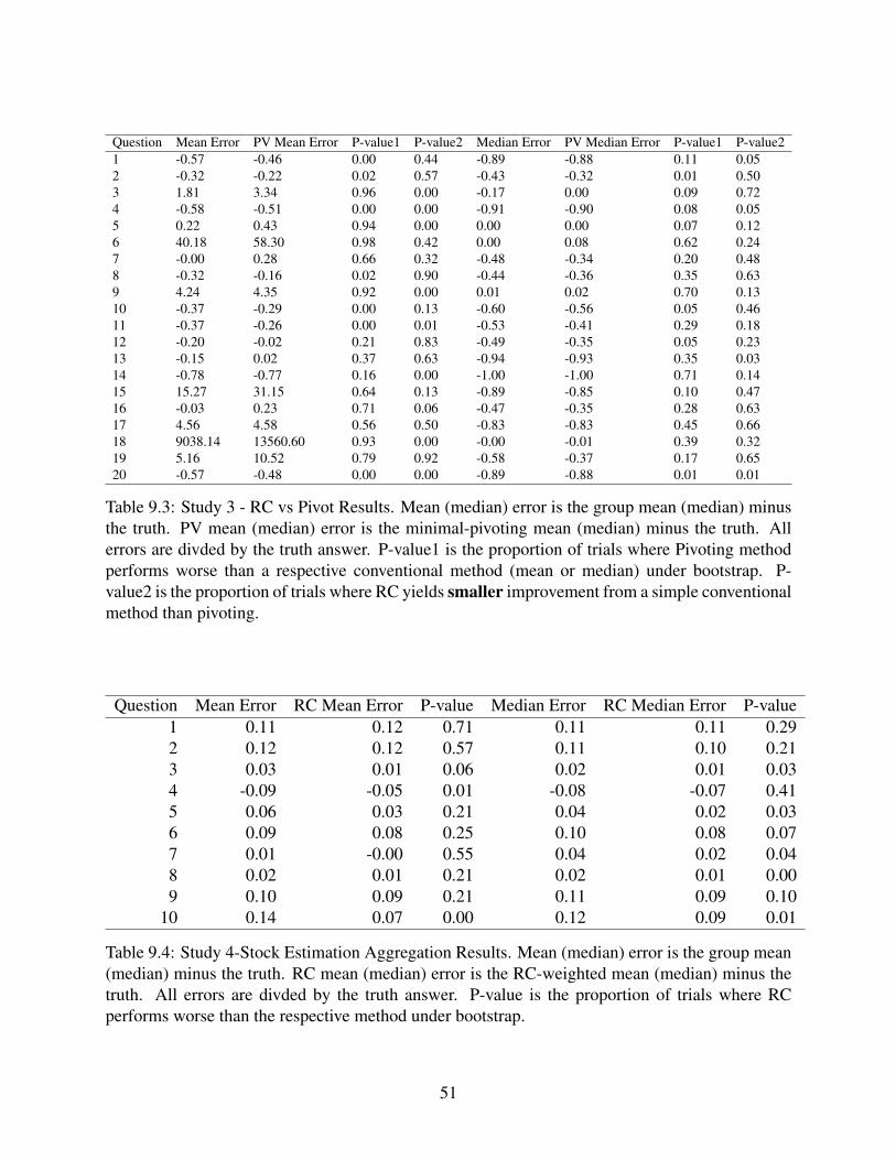
Question Mean Error PV Mean Error P-value1 P-value2 Median Error PV Median Error P-value1 P-value21 -0.57 -0.46 0.00 0.44 -0.89 -0.88 0.11 0.052 -0.32 -0.22 0.02 0.57 -0.43 -0.32 0.01 0.503 1.81 3.34 0.96 0.00 -0.17 0.00 0.09 0.724 -0.58 -0.51 0.00 0.00 -0.91 -0.90 0.08 0.055 0.22 0.43 0.94 0.00 0.00 0.00 0.07 0.126 40.18 58.30 0.98 0.42 0.00 0.08 0.62 0.247 -0.00 0.28 0.66 0.32 -0.48 -0.34 0.20 0.488 -0.32 -0.16 0.02 0.90 -0.44 -0.36 0.35 0.639 4.24 4.35 0.92 0.00 0.01 0.02 0.70 0.1310 -0.37 -0.29 0.00 0.13 -0.60 -0.56 0.05 0.4611 -0.37 -0.26 0.00 0.01 -0.53 -0.41 0.29 0.1812 -0.20 -0.02 0.21 0.83 -0.49 -0.35 0.05 0.2313 -0.15 0.02 0.37 0.63 -0.94 -0.93 0.35 0.0314 -0.78 -0.77 0.16 0.00 -1.00 -1.00 0.71 0.1415 15.27 31.15 0.64 0.13 -0.89 -0.85 0.10 0.4716 -0.03 0.23 0.71 0.06 -0.47 -0.35 0.28 0.6317 4.56 4.58 0.56 0.50 -0.83 -0.83 0.45 0.6618 9038.14 13560.60 0.93 0.00 -0.00 -0.01 0.39 0.3219 5.16 10.52 0.79 0.92 -0.58 -0.37 0.17 0.6520 -0.57 -0.48 0.00 0.00 -0.89 -0.88 0.01 0.01

Table 9.3: Study 3 - RC vs Pivot Results. Mean (median) error is the group mean (median) minusthe truth. PV mean (median) error is the minimal-pivoting mean (median) minus the truth. Allerrors are divded by the truth answer. P-value1 is the proportion of trials where Pivoting methodperforms worse than a respective conventional method (mean or median) under bootstrap. P-value2 is the proportion of trials where RC yields smaller improvement from a simple conventionalmethod than pivoting.

Question Mean Error RC Mean Error P-value Median Error RC Median Error P-value1 0.11 0.12 0.71 0.11 0.11 0.292 0.12 0.12 0.57 0.11 0.10 0.213 0.03 0.01 0.06 0.02 0.01 0.034 -0.09 -0.05 0.01 -0.08 -0.07 0.415 0.06 0.03 0.21 0.04 0.02 0.036 0.09 0.08 0.25 0.10 0.08 0.077 0.01 -0.00 0.55 0.04 0.02 0.048 0.02 0.01 0.21 0.02 0.01 0.009 0.10 0.09 0.21 0.11 0.09 0.10

10 0.14 0.07 0.00 0.12 0.09 0.01

Table 9.4: Study 4-Stock Estimation Aggregation Results. Mean (median) error is the group mean(median) minus the truth. RC mean (median) error is the RC-weighted mean (median) minus thetruth. All errors are divded by the truth answer. P-value is the proportion of trials where RCperforms worse than the respective method under bootstrap.

51

Chapter 10

Bibliography

1. David V. Budescu, Eva Chen (2015) Identifying Expertise to Extract the Wisdom of Crowds.Management Science 61(2):267-280. https://doi.org/10.1287/mnsc.2014.1909

2. Mannes, A. E., Soll, J. B., & Larrick, R. P. (2014). The wisdom of select crowds. Journal ofPersonality and Social Psychology, 107, 276-299.

3. Stefano DellaVigna & Devin Pope, 2018. "What Motivates Effort? Evidence and ExpertForecasts," Review of Economic Studies, Oxford University Press, vol. 85(2), pages 1029-1069.

4. Prelec, D. (2004). A Bayesian truth serum for subjective data. Science 306 (5695),462466.

5. Miller, N., P. Resnick, and R. Zeckhauser (2005). Eliciting informative feedback: The peer-prediction method. Management Science 51 (9), 13591373.

6. Aidan Lyon, Bonnie C. Wintle, Mark Burgman (2015) Collective wisdom: Methods ofconfidence interval aggregation, Journal of Business Research, Volume 68, Issue 8, 2015, Pages1759-1767, ISSN 0148-2963, https://doi.org/10.1016/j.jbusres.2014.08.012.

7. Koriat, A., & Adiv, S. (2016). The self-consistency theory of subjective confidence. InJ. Dunlosky & S. K. Tauber (Eds.), Oxford library of psychology. The Oxford handbook ofmetamemory (pp. 127-147). New York, NY, US: Oxford University Press.

8. Koriat, A. (2008). Subjective confidence in one’s answers: The consensuality principle.Journal of Experimental Psychology: Learning, Memory, and Cognition, 34(4), 945-959.

9. Moore, D. A. and P. J. Healy (2008). The trouble with overcondence. Psychological Review 115 (2), 502.

10. Malmendier, Ulrike, and Timothy Taylor. 2015. "On the Verges of Overconfidence." Jour-

52

nal of Economic Perspectives, 29 (4): 3-8.

11. Moore, Don & Swift, Samuel & Minster, Angela & Mellers, Barbara & Ungar, Lyle & Tet-lock, Philip & Yang, Heather & Tenney, Elizabeth. (2017). Confidence Calibration in a MultiyearGeopolitical Forecasting Competition. Management Science. 63. 3552-3565.

12. Prelec, D., Seung, H.S., & McCoy, J. (2017). A solution to the single-question crowdwisdom problem. Nature, 541, 532-535.

13. Manski, C. F. and C. Neri (2013). First- and second-order subjective expectations in strate-gic decision-making: Experimental evidence. Games and Economic Behavior

14. Becker, G. M., M. H. DeGroot, and J. Marschak (1964). Measuring utility by a single-response sequential method. Behavioral Science 9 (3), 226232.

15. Lorenz, J., Rauhut, H., Schweitzer, F., & Helbing, D. (2011). How social influence canundermine the wisdom of crowd effect. Proceedings of the National Academy of Sciences of theUnited States of America, 108(22), 9020–9025. doi:10.1073/pnas.1008636108

16. Karni, E. (2009). A mechanism for eliciting probabilities. Econometrica 77 (2), 603-606.

17. Karni, E. (2018). A mechanism for eliciting second-order beliefs and the inclination tochoose. American Economic Journal: Microeconomics.

18. D. Kreps, A representation theorem for “Preference for flexibility”, Econometrica 47(1979) 565–577.

19. David Dillenberger, Juan Sebastián Lleras, Philipp Sadowski, Norio Takeoka, A theory ofsubjective learning, Journal of Economic Theory, Volume 153, 2014, Pages 287-312,ISSN 0022-0531, https://doi.org/10.1016/j.jet.2014.07.003.

20. F.J. Anscombe, R.J. Aumann, A definition of subjective probability, Ann. Math. Stat. 34(1963) 199–205.

21. J. Savage, The Foundations of Statistics, John Wiley & Sons, New York, 1954.

22. Hong, L. & Page, S. E., Problem Solving by Heterogeneous Agents1, J. Econ. Theory. 97(2001), 123–163.

23. Ilan Yaniv, Receiving other people’s advice: Influence and benefit, Organizational Be-havior and Human Decision Processes, Volume 93, Issue 1, 2004, Pages 1-13, ISSN 0749-5978,https://doi.org/10.1016/j.obhdp.2003.08.002.

24. Schultze, T., Rakotoarisoa, A., & Schulz-Hardt, S. (2015). Effects of distance betweeninitial estimates and advice on advice utilization. Judgment and Decision Making, 10, 144-171.

53

25. Ravazzolo, F., & Røisland, Ø. (2011). Why do people place lower weight on advice farfrom their own initial opinion? Economics Letters, 112(1), 63–66.

26. J Ugander, R Drapeau, C Guestrin (2015) The Wisdom of Multiple Guesses Proc. 16thACM Conf. on Economics and Computation (EC), 2015.

27. Moshe Leshno, Yishay Spector, An elementary proof of Blackwell’s theorem, Mathemati-cal Social Sciences, Volume 25, Issue 1, 1992, Pages 95-98, ISSN 0165-4896

28. Blackwell David, “Comparison of Experiments,” in Jerzy Neyman, ed., Proceedings of theSecond Berkeley Symposium on Mathematical Statistics and Probability, University of CaliforniaPress Berkeley, CA 1951, pp. 93–102.

29. Chambers, Christopher P., and Nicholas S. Lambert. 2018. “Dynamic Belief Elicitation.”Conditionally Accepted by Econometrica

30. Frankel, Alexander, and Emir Kamenica. 2019. "Quantifying Information and Uncer-tainty." American Economic Review, 109 (10): 3650-80.

31. Jian Li, Junjie Zhou, Blackwell’s informativeness ranking with uncertainty-averse prefer-ences, Games and Economic Behavior, Volume 96, 2016, Pages 18-29

54