water

Article

Identification of the Optimum Rain Gauge NetworkDensity for Hydrological Modelling Based on RadarRainfall Analysis

Yeboah Gyasi-Agyei

School of Engineering and Technology, Central Queensland University, Bruce Highway,Rockhampton, QLD 4702, Australia; y.gyasi-agyei@cqu.edu.au; Tel.: +61-408-30-9977

Received: 10 June 2020; Accepted: 30 June 2020; Published: 3 July 2020�����������������

Abstract: Rain gauges continue to be sources of rainfall data despite progress made in precipitationmeasurements using radar and satellite technology. There has been some work done on assessing theoptimum rain gauge network density required for hydrological modelling, but without consensus.This paper contributes to the identification of the optimum rain gauge network density, using scalinglaws and bias-corrected 1 km × 1 km grid radar rainfall records, covering an area of 28,371 km2

that hosts 315 rain gauges in south-east Queensland, Australia. Varying numbers of radar pixels(rain gauges) were repeatedly sampled using a unique stratified sampling technique. For each set ofrainfall sampled data, a two-dimensional correlogram was developed from the normal scores obtainedthrough quantile-quantile transformation for ordinary kriging which is a stochastic interpolation.Leave-one-out cross validation was carried out, and the simulated quantiles were evaluated usingthe performance statistics of root-mean-square-error and mean-absolute-bias, as well as their ratesof change. A break in the scaling of the plots of these performance statistics against the number ofrain gauges was used to infer the optimum rain gauge network density. The optimum rain gaugenetwork density varied from 14 km2/gauge to 38 km2/gauge, with an average of 25 km2/gauge.

Keywords: rain gauge; network density; rainfall; radar; kriging; stochastic interpolation; scaling

1. Introduction

Rainfall is a key forcing input for hydrological modelling, such as that used in studies on extremeevents and climate impact analysis. However, the high spatial variability of rainfall is recognised,and thus data regarding the rainfall distribution in space and time is paramount for meaningful useof the outputs of hydrological models. Ground-based rain gauges have been the source of rainfallmeasurement for quite a long time, and are generally seen as the “ground truth”. However, the poorgauge network density, as a result of limited resources, accessibility and maintenance [1], is a challenge.This is coupled with the fact that gauges provide information for a small area (e.g., 203 mm indiameter), and extrapolating to the spatial scale of several km2 introduces high uncertainty (e.g., [2]).In recent years, gridded radar and satellite products data have been processed to obviate the limitationsof the gauges, but these approaches have their challenges, including the spatial scale, which rangesfrom 1 km2 to about 50 km2. The systematic bias issues that these products suffer range from sensorlimitations to sampling errors and the algorithms for retrieval [3]). Although weather radar capturesvery well the spatial variability, the intensities suffer uncertainties stemming from factors such as beamblocking, ground clutter and signal attenuation [4]. As such, there is always the need to bias-correctthese data sources with reference to the gauged measurements, and thus point rain gauge recordsand interpolation methods will continue to play a key role in hydrological modelling. This obviously

Water 2020, 12, 1906; doi:10.3390/w12071906 www.mdpi.com/journal/water

Water 2020, 12, 1906 2 of 19

means that the combination of rain gauge records with either radar and/or satellite products willcontinue to be widely used, except for in regions without radar or satellite data [5].

Gridded rainfall products (satellite, radar, general circulation models (GCMs), regional climatemodels (RCMs) are normally calibrated and validated using rain gauge data, but the poor networkdensity introduces a high degree of uncertainty [6]. It is not just the density of the rain gauge networks,but their non-uniform (irregular) distribution over the catchments, due to issues of accessibility andtopography, among other factors, also contribute to the uncertainty [7], bearing in mind the hightemporal and spatial variability [8]. Studies on the effects of rain gauge distribution and density oninput rainfall and hydrological modelling have highlighted that the key factor in runoff errors is theerrors in the input rainfall [9,10].

There have been numerous studies to identify the optimum rain gauge density, but without aconsensus being reached. As summarised in [11], there is great variation in the studied catchmentsizes and the rain gauge densities used in the various studies. For example, [12] used 10 gauges ina < 0.05-km2 (0.005 km2/gauge) catchment, whereas [10] used 60 gauges in a 6400-km2 study area.Most of the studies focused on the effect of changing the number of rain gauges on runoff response,and not necessarily on identifying the optimum rain gauge network density [13]. By reducing thenumber of rain gauges from seven to 1 in a 0.5◦ × 0.5◦ grid box, Mishra [14] observed that the absoluteerror in daily rainfall measurement was reduced by 49%.

Approaches in the literature that improve the quality of satellite and radar rainfall products includethe simple scaling method (e.g., [15]). This method corrects the mean values of the gridded data based onbias factors of the gridded and observed data, calculated at the monthly or daily timescale. This methodwas slightly modified to improve the variance as well, by introducing a power law correction [16].A major disadvantage of these methods is their failure to leverage the spatial and temporal patterns inthe observed data. Quantile mapping (QM) (e.g., [17]) is another popular method that only correctsthe marginal distribution, without regard for the spatial connectivity (spatial structure), or the wet-and dry-spell lengths and the transition probability that describe the temporal sequences. Essentially,it transforms the gridded data in order to preserve the marginal distribution of the observed data [18].Yang et al. [3] presented a framework that uses a Gaussian weighting (GW) interpolation QM approach,in order to bias-correct the PERSIANN-CCS satellite precipitation product over Chile. Bias-correctionmethods have been applied to GCMs/RCMs outputs [19,20] as well. These methods are based on theassumption that the observed data provide the population distribution, while it is in actuality only asample of the population, as demonstrated in this paper.

A framework for generating daily rainfields, based on interpolation of point data [21–24], is adoptedfor the analysis in this paper. The daily radar rainfall data is bias-corrected using the observed data,before using a stratified sampling approach to sample a given number of rain gauge locations. A majorcontribution of the paper is the recognition that the marginal distribution of the observed daily data isjust a sample, and the population distribution needs to be identified through a bias-correction procedure.In addition, the spatial structure of the radar rainfield was considered as the best representation,but its marginal distribution for the day was bias-corrected. In essence, it is assumed that radarprovides the best spatial structure, and the point rain gauges the true intensities. Given a set of pointlocations in a catchment, a two-dimensional (2D) correlogram is developed and used in an ordinarykriging stochastic interpolation. Leave-one-out cross validation (LOOCV) is used to estimate theperformance statistics for a given set of rain gauge numbers. A break in scaling, identified by plots ofthe performance statistics and the number of rain gauges, was used to infer the optimum rain gaugenetwork density, which is the main aim of this paper.

2. Study Area and Data

The study area is part of a 128-km radius circular range of the Mt. Stapylton weather radar station,which has a landfall area of 28,371 km2 (Figure 1).

Water 2020, 12, 1906 3 of 19

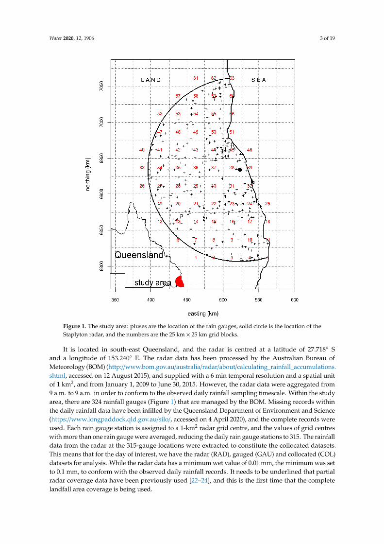
Figure 1. The study area: pluses are the location of the rain gauges, solid circle is the location of theStaplyton radar, and the numbers are the 25 km × 25 km grid blocks.

It is located in south-east Queensland, and the radar is centred at a latitude of 27.718◦ Sand a longitude of 153.240◦ E. The radar data has been processed by the Australian Bureau ofMeteorology (BOM) (http://www.bom.gov.au/australia/radar/about/calculating_rainfall_accumulations.shtml, accessed on 12 August 2015), and supplied with a 6 min temporal resolution and a spatial unitof 1 km2, and from January 1, 2009 to June 30, 2015. However, the radar data were aggregated from9 a.m. to 9 a.m. in order to conform to the observed daily rainfall sampling timescale. Within the studyarea, there are 324 rainfall gauges (Figure 1) that are managed by the BOM. Missing records withinthe daily rainfall data have been infilled by the Queensland Department of Environment and Science(https://www.longpaddock.qld.gov.au/silo/, accessed on 4 April 2020), and the complete records wereused. Each rain gauge station is assigned to a 1-km2 radar grid centre, and the values of grid centreswith more than one rain gauge were averaged, reducing the daily rain gauge stations to 315. The rainfalldata from the radar at the 315-gauge locations were extracted to constitute the collocated datasets.This means that for the day of interest, we have the radar (RAD), gauged (GAU) and collocated (COL)datasets for analysis. While the radar data has a minimum wet value of 0.01 mm, the minimum was setto 0.1 mm, to conform with the observed daily rainfall records. It needs to be underlined that partialradar coverage data have been previously used [22–24], and this is the first time that the completelandfall area coverage is being used.

Water 2020, 12, 1906 4 of 19

A temperate climate, without a dry season and a hot summer, characterises the climate ofthe study area, in accordance with the classification of [25]. It is a subtropical region, with anaverage temperature of 26.5 ◦C, and with summer temperatures sometimes exceeding 29 ◦C.The region experiences an average annual rainfall of 990 mm, the majority of which occurs during thesummer months, from December to March. The winter months from June to August are generally dry,whereas the hot summer months from December to February could experience elevated numbersof thunderstorms.

3. Methodology

3.1. Marginal Distribution Fitting

A standard two-parameter right-skewed distribution is fitted to the daily rainfall amounts greaterthan zero from the 3 datasets (RAD, GAU and COL) separately. One standard distribution is chosenfrom the set of Generalized Pareto, Gamma, Gumbel, Log-Logistic, Log-Normal, Kappa and Weibull(R packages fitdistrplus, [26]; FAdist, [27]), using the Anderson-Darling statistic. These right-skeweddistributions are considered appropriate for daily rainfall amounts as treated here, and they arecommonly used in the literature [28–32]. The fitted distribution is used to transform the daily amountsto probabilities, and then to the standard Gaussian (N [0,1]) quantiles (Q-Q transformation) used in theordinary kriging interpolation. However, there is a need to account for the dry gauges (zeros) thatabound in daily rainfall records. Daily rainfall amounts r at a dry station k with spatial coordinates Skare assigned as:

r[sk] = 0.1 exp(−

d[sk]

d

)(1)

where d[sk] is the minimum distance of the dry gauge located at Sk from a wet gauge, d is the averageof d, and 0.1 is the minimum wet gauge value. Assuming po represents the proportion of the gaugesthat are dry, the fitted two-parameter distribution FR is zero inflated and used to transform the rainfallamounts r[sk] into standard Gaussian quantiles (normal score) w[sk], as:

w[sk] =Φ−1[FR(r[sk])(1− p0) + p0] , r[sk] ≥ 0.1

Φ−1[p0. exp

(−

d[sk]

d

)], r[sk] < 0.1

(2)

In Equation (2), the cumulative normal distribution N [0,1] is represented as Φ, and Φ−1 isthe inverse. Given a normal score, the inverse of Equation (2), written as

r[sk] =F−1

R [{Φ(w[sk]) − p0

}/(1− p0)] , Φ(w[sk]) ≥ p0

0 , Φ(w[sk]) < p0(3)

gives the rainfall amount.

3.2. Bias Correction

There could be significant differences between the marginal distributions of GAU, RAD andCOL datasets for the same day. Hence a bias correction method was implemented. The traditionalQuantile-Quantile (Q-Q) bias-correction method assumes that the observed gauge data provide theright distribution, and that the gridded datasets from radar, satellite or GCMs/RCMs therefore need tobe adjusted to reflect the observed distribution. This idea is expressed mathematically as (e.g., [18])

RRAD−BC = F−1GAU[FRAD(RRAD)] (4)

and is used to correct the gridded radar rainfall amounts (RRAD) to bias-corrected (RRAD−BC) amounts,using the rain gauge data distribution (FGAU) and radar data distribution (FRAD) for the day, F−1 being

Water 2020, 12, 1906 5 of 19

the inverse function. However, the observed daily records as used in this paper are seen as a sample,and therefore require adjustment as well. As presented later, the number of rain gauges is not highenough to reproduce the spatial structure for a wet day.

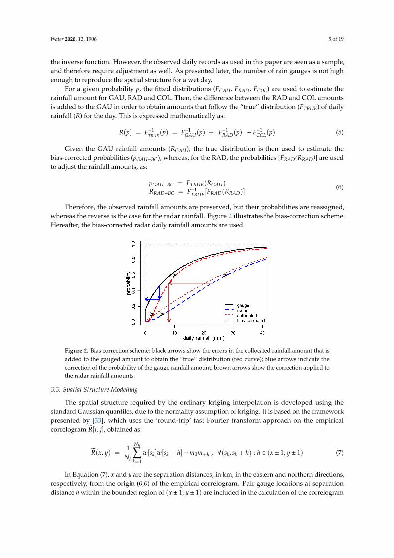
For a given probability p, the fitted distributions (FGAU, FRAD, FCOL) are used to estimate therainfall amount for GAU, RAD and COL. Then, the difference between the RAD and COL amountsis added to the GAU in order to obtain amounts that follow the “true” distribution (FTRUE) of dailyrainfall (R) for the day. This is expressed mathematically as:

R(p) = F−1TRUE

(p) = F−1GAU(p) + F−1

RAD(p) − F−1COL(p) (5)

Given the GAU rainfall amounts (RGAU), the true distribution is then used to estimate thebias-corrected probabilities (pGAU−BC), whereas, for the RAD, the probabilities [FRAD(RRAD)] are usedto adjust the rainfall amounts, as:

pGAU−BC = FTRUE(RGAU)

RRAD−BC = F−1TRUE[FRAD(RRAD)]

(6)

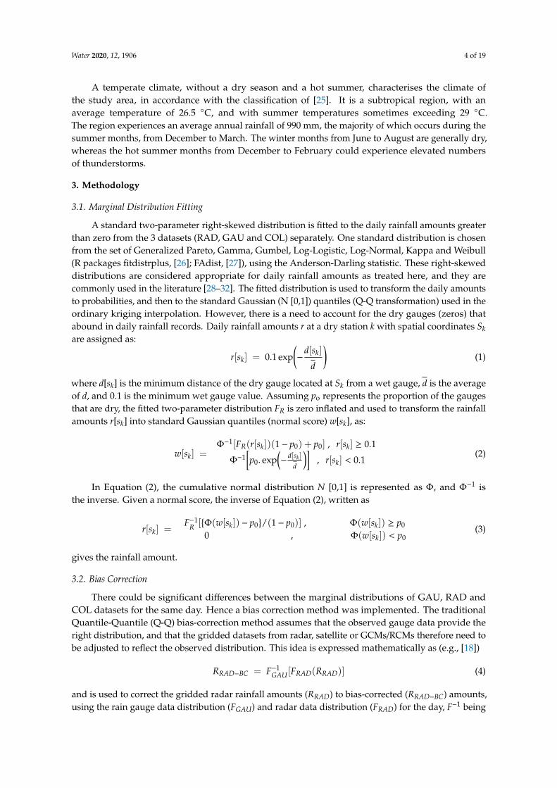
Therefore, the observed rainfall amounts are preserved, but their probabilities are reassigned,whereas the reverse is the case for the radar rainfall. Figure 2 illustrates the bias-correction scheme.Hereafter, the bias-corrected radar daily rainfall amounts are used.

Figure 2. Bias correction scheme: black arrows show the errors in the collocated rainfall amount that isadded to the gauged amount to obtain the “true” distribution (red curve); blue arrows indicate thecorrection of the probability of the gauge rainfall amount; brown arrows show the correction applied tothe radar rainfall amounts.

3.3. Spatial Structure Modelling

The spatial structure required by the ordinary kriging interpolation is developed using thestandard Gaussian quantiles, due to the normality assumption of kriging. It is based on the frameworkpresented by [33], which uses the ‘round-trip’ fast Fourier transform approach on the empiricalcorrelogram R̃[i, j], obtained as:

R̃(x, y) =1

Nh

Nh∑k=1

w[sk]w[sk + h] −m0m+h , ∀(sk, sk + h) : h ∈ (x± 1, y± 1) (7)

In Equation (7), x and y are the separation distances, in km, in the eastern and northern directions,respectively, from the origin (0,0) of the empirical correlogram. Pair gauge locations at separationdistance h within the bounded region of (x± 1, y± 1) are included in the calculation of the correlogram

Water 2020, 12, 1906 6 of 19

value at the grid point (x, y), with Nh representing the number of pair gauges. The means of the pair oftail w[sk] and head w[sk + h] values are denoted as mo and m+h, respectively.

Following [21,22], a 2D exponential distribution expressed as

RΘ(x, y) = RΘ(u, v) = exp

−[( u

Lu

)2+

( vLv

)2]1/2

,u = y sin(θ) + x cos(θ)v = y cos(θ) − x sin(θ)

(8)

was fitted to the empirical correlogram data. Along an elliptical contour, u and v are the separationdistances in the direction of the major and minor axes, respectively. The 3 parameters defining the2D exponential distribution are the angle between the major axis and the horizontal direction (θ),the major axis length (Lu), and the minor axis length (Lv), the anisotropy ratio (η) being definedas Lv/Lu. These parameters are estimated using the global optimisation technique of [34] by matchingthe empirical and the analytical elliptical correlogram contours [21].

3.4. Stratified Sampling of Rain Gauge Locations

In order to investigate the effects of the number of rain gauges (radar pixels used interchangeably)on the spatial structure, a set number of rain gauges were sampled from the grid centres of theradar data. It is a known fact that rain gauges are by no means uniformly distributed over astudy region, as exemplified in Figure 1 for the study region. Therefore, a stratified sampling approachwas adopted to mimic the spatial distribution of the current rain gauges. These are the steps for thestratified sampling approach:

• Firstly, the study region was overlaid with a 25 km× 25 km grid, and the resulting 63 blocks within,or intersecting, the study region are labelled in Figure 1;

• Secondly, rain gauges within each grid were counted, and those blocks devoid of gauges wereassigned a value of 0.5 times the fraction of the grid within the radar coverage, to allow forpossible selection of gauges within the fractional grids, particularly for higher sampling numbers.The rain gauge network density of the grids varies from 1.7 to 48.6 gauges per 1000 km2, grid 45recording the highest density;

• Thirdly, the observed rain gauge counts within the grids were used to develop the weights for thestratified sampling;

• Fourth, the number of rain gauges required were sampled with replacement from integers 1 to 63,representing the grids, in accordance with their weights;

• Finally, the numbers of samples from each grid from the previous step were sampled randomly,without replacement from the subset of the grid, noting that the subset of each grid is the numberof 1-km2 radar grid centres it contains, which varies from 6 (grid 61) to 625 (the inner grids).

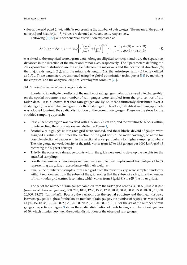
The set of the number of rain gauges sampled from the radar grid centres is {20, 50, 100, 200, 315(number of observed gauges), 500, 750, 1000, 1250, 1500, 1750, 2000, 3000, 5000, 7500, 10,000, 15,000,20,000, 28,371 (full radar)}. Because the variability in the spatial structure and the mean distancebetween gauges is highest for the lowest number of rain gauges, the number of repetitions was variedas {50, 45, 40, 35, 30, 25, 20, 20, 20, 20, 20, 20, 20, 20, 20, 20, 10, 10, 1} for the set of the number of raingauges, respectively. Figure 3 shows the spatial distribution of 3 sets having a number of rain gaugesof 50, which mimics very well the spatial distribution of the observed rain gauges.

Water 2020, 12, 1906 7 of 19

Figure 3. Distribution of 3 sets of 50 rain gauge locations selected by the stratified sampling approach.

3.5. Performance Statistics

Ordinary kriging does not require a description here, as it has been well documented in theliterature (e.g., [35,36]). However, it suffices to say that it estimates a variable at a target locationusing known values at several locations in space, and it is based on linear weighted least squares.For each set of a number of rain gauges sampled, one of the distributions discussed in Section 3.1 wasfitted and used to convert the rainfall amounts to standard normal quantiles by means of Equation (2).Then, a 2D correlogram was fitted as explained in Section 3.3. Next, leave-one-out cross validation(LOOCV) was performed using the R package gstat [37]. LOOCV leaves one data point out at a time,and its prediction is made using the remaining data points. The predictions in the normal score wereconverted to rainfall amounts using Equation (3). The predicted values were evaluated using theroot-mean-square-error (RMSE) and the mean-absolute-bias (MAB) performance statistics, defined as:

RMSE =

√√√1N

N∑i=1

[VO(i) −VP(i)]2 (9)

MAB =1N

N∑i=1

∣∣∣VO(i) −VP(i)∣∣∣ (10)

where the observed and predicted values for the ith gauge are, respectively, VO(i) and VP(i), and N isthe number of sampled rain gauges. The variation of the performance statistics with the number ofrain gauges is used to identify the optimum rain gauge network density.

Water 2020, 12, 1906 8 of 19

4. Results and Discussion

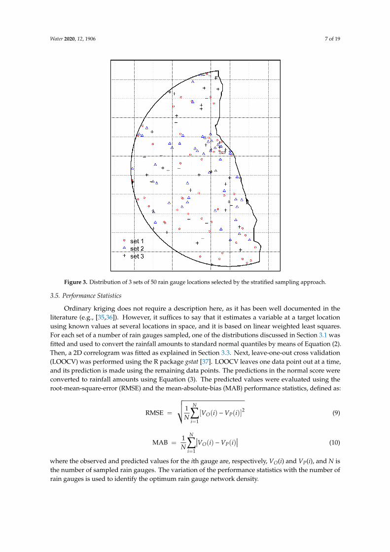
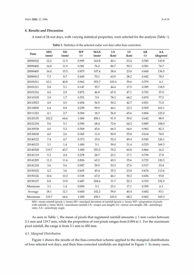
A total of 24 wet days, with varying statistical properties, were selected for the analysis (Table 1).

Table 1. Statistics of the selected radar wet days after bias correction.

DateMN SD WP MAX LX LY AR AA

(mm) (mm) (-) (mm) (km) (km) (-) (degrees)

20090102 12.2 11.5 0.995 163.8 40.1 23.4 0.583 143.8

20090402 16.8 11.9 0.381 76.2 86.7 50.3 0.581 74.7

20090405 16.0 15.5 0.875 107.4 38.4 23.0 0.600 136.5

20090413 7.3 8.7 0.445 70.1 63.9 28.2 0.442 78.3

20101011 63.1 40.8 0.962 353.7 103.0 59.6 0.579 6.1

20101211 5.8 5.1 0.147 35.7 44.4 17.5 0.395 118.5

20101216 4.6 2.9 0.872 46.8 67.0 47.1 0.703 37.0

20110105 3.9 1.7 0.551 5.9 78.3 68.2 0.870 77.5

20110523 4.9 4.5 0.454 56.5 50.2 42.7 0.851 71.0

20110830 6.4 8.9 0.258 99.9 44.1 22.3 0.505 163.1

20111223 4.1 2.7 0.094 18.3 56.8 45.6 0.804 122.0

20120125 102.2 64.6 1.000 450.1 91.9 59.0 0.642 98.9

20121218 5.6 5.1 0.590 68.4 72.6 64.2 0.885 108.0

20130530 4.0 5.2 0.509 45.6 66.5 64.0 0.962 82.3

20130630 4.0 2.6 0.365 11.0 90.9 55.8 0.614 74.9

20140122 7.4 4.7 0.373 15.0 52.4 49.4 0.943 126.1

20140123 3.1 1.4 1.000 5.1 59.0 31.4 0.533 169.3

20140328 119.7 43.7 1.000 353.2 70.2 60.8 0.866 16.2

20141119 5.3 4.4 0.278 28.7 23.1 17.1 0.739 17.0

20141205 11.2 11.6 0.826 65.2 49.3 35.6 0.722 120.3

20141218 3.6 5.6 0.987 59.5 53.3 27.6 0.517 33.4

20150102 4.2 3.6 0.605 45.4 35.3 23.8 0.674 113.6

20150126 10.6 10.2 0.338 67.0 46.1 30.2 0.656 93.8

20150127 8.8 13.9 0.487 204.6 31.7 22.3 0.703 152.5

Minimum 3.1 1.4 0.094 5.1 23.1 17.1 0.395 6.1

Average 18.1 12.1 0.600 102.2 59.0 40.4 0.682 93.1

Maximum 119.7 64.6 1.000 450.1 103.0 68.2 0.962 169.3

MN—mean rainfall (pixels ≥ 1mm); SD—standard deviation of rainfall (pixels ≥ 1mm); WP—proportion of pixelswith rainfall ≥ 1mm; MAX—maximum rainfall; LX—major axis length; LY—minor axis length; AR—anisotropyratio; AA—anisotropy angle.

As seen in Table 1, the mean of pixels that registered rainfall amounts ≥ 1 mm varies between3.1 mm and 119.7 mm, while the proportion of wet pixels ranges from 0.094 to 1. For the maximumpixel rainfall, the range is from 5.1 mm to 450 mm.

4.1. Marginal Distribution

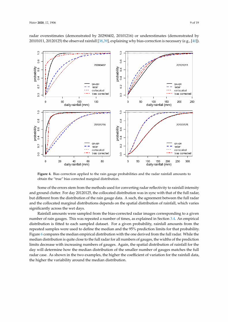
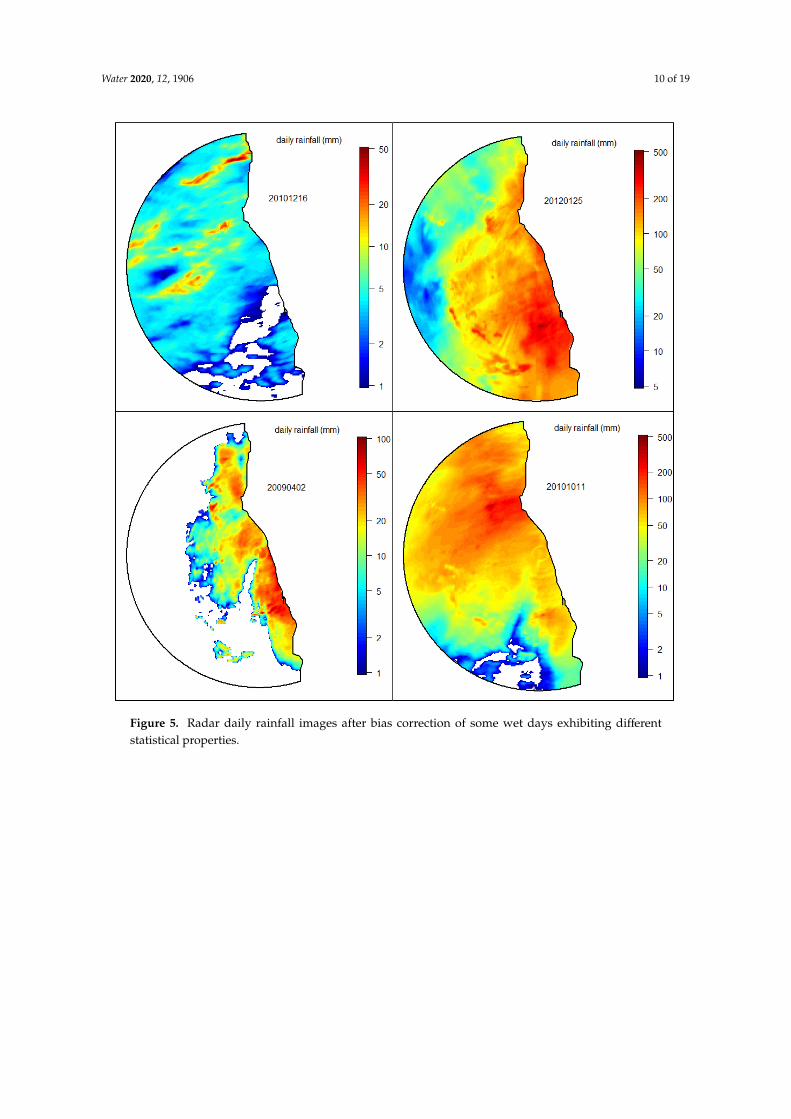
Figure 4 shows the results of the bias-correction scheme applied to the marginal distributionsof four selected wet days, and their bias-corrected rainfields are depicted in Figure 5. In many cases,

Water 2020, 12, 1906 9 of 19

radar overestimates (demonstrated by 20290402, 20101216) or underestimates (demonstrated by20101011, 20120125) the observed rainfall [38,39], explaining why bias-correction is necessary (e.g., [40]).

Figure 4. Bias correction applied to the rain gauge probabilities and the radar rainfall amounts toobtain the “true” bias corrected marginal distribution.

Some of the errors stem from the methods used for converting radar reflectivity to rainfall intensityand ground clutter. For day 20120125, the collocated distribution was in sync with that of the full radar,but different from the distribution of the rain gauge data. A such, the agreement between the full radarand the collocated marginal distributions depends on the spatial distribution of rainfall, which variessignificantly across the wet days.

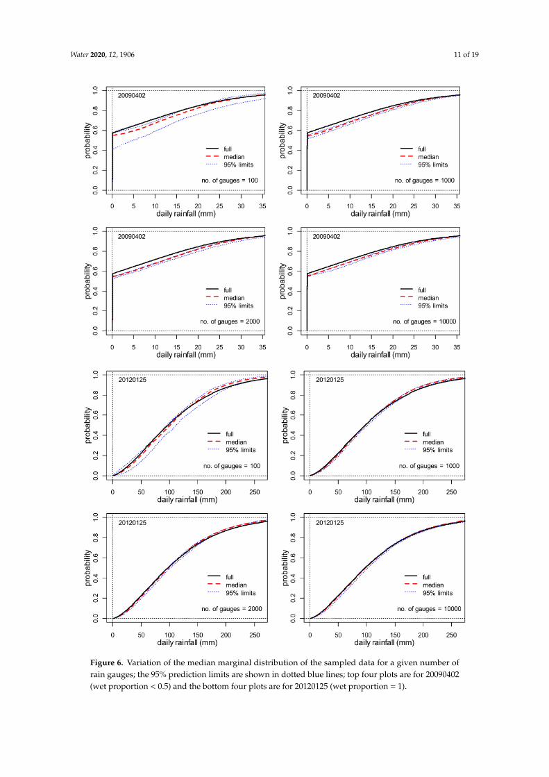
Rainfall amounts were sampled from the bias-corrected radar images corresponding to a givennumber of rain gauges. This was repeated a number of times, as explained in Section 3.4. An empiricaldistribution is fitted to each sampled dataset. For a given probability, rainfall amounts from therepeated samples were used to define the median and the 95% prediction limits for that probability.Figure 6 compares the median empirical distribution with the one derived from the full radar. While themedian distribution is quite close to the full radar for all numbers of gauges, the widths of the predictionlimits decrease with increasing numbers of gauges. Again, the spatial distribution of rainfall for theday will determine how the median distribution of the smaller number of gauges matches the fullradar case. As shown in the two examples, the higher the coefficient of variation for the rainfall data,the higher the variability around the median distribution.

Water 2020, 12, 1906 10 of 19

Figure 5. Radar daily rainfall images after bias correction of some wet days exhibiting differentstatistical properties.

Water 2020, 12, 1906 11 of 19

Figure 6. Variation of the median marginal distribution of the sampled data for a given number ofrain gauges; the 95% prediction limits are shown in dotted blue lines; top four plots are for 20090402(wet proportion < 0.5) and the bottom four plots are for 20120125 (wet proportion = 1).

Water 2020, 12, 1906 12 of 19

4.2. Spatial Structure Parameters

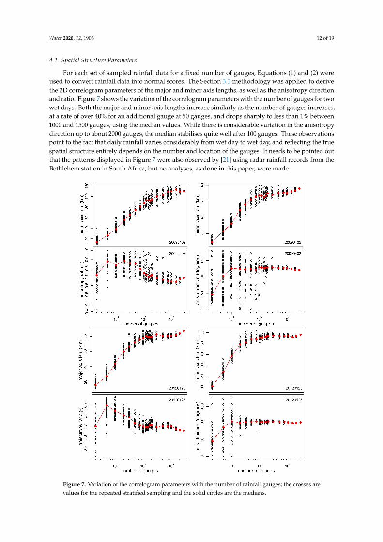
For each set of sampled rainfall data for a fixed number of gauges, Equations (1) and (2) wereused to convert rainfall data into normal scores. The Section 3.3 methodology was applied to derivethe 2D correlogram parameters of the major and minor axis lengths, as well as the anisotropy directionand ratio. Figure 7 shows the variation of the correlogram parameters with the number of gauges for twowet days. Both the major and minor axis lengths increase similarly as the number of gauges increases,at a rate of over 40% for an additional gauge at 50 gauges, and drops sharply to less than 1% between1000 and 1500 gauges, using the median values. While there is considerable variation in the anisotropydirection up to about 2000 gauges, the median stabilises quite well after 100 gauges. These observationspoint to the fact that daily rainfall varies considerably from wet day to wet day, and reflecting the truespatial structure entirely depends on the number and location of the gauges. It needs to be pointed outthat the patterns displayed in Figure 7 were also observed by [21] using radar rainfall records from theBethlehem station in South Africa, but no analyses, as done in this paper, were made.

Figure 7. Variation of the correlogram parameters with the number of rainfall gauges; the crosses arevalues for the repeated stratified sampling and the solid circles are the medians.

Water 2020, 12, 1906 13 of 19

4.3. The Optimum Rain Gauge Network Density

In this section, each set of sampled rainfall data for a fixed number of gauges is used to developthe marginal distribution and the 2D spatial structure required by the ordinary kriging interpolation.The LOOCV technique was used to simulate rainfall amounts, which were evaluated using RMSEand MAB, as presented in Section 3.5, thus incorporating uncertainties into the marginal distributionand the 2D spatial structure, because of the inadequate number of gauges sampled.

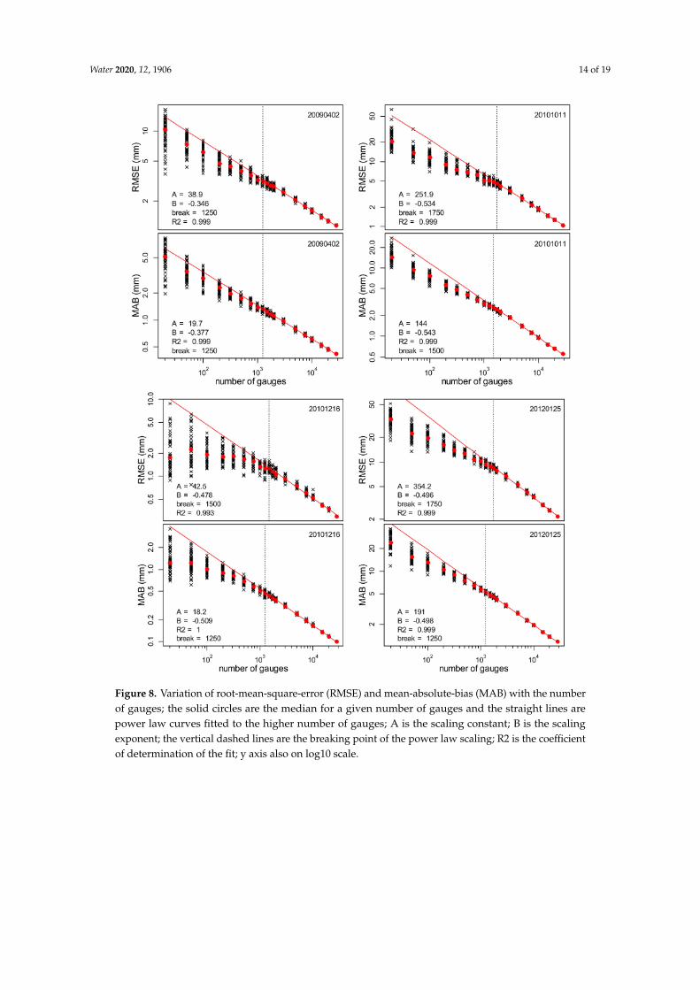
Figure 8 shows plots of the performance statistics (RMSE and MAB) against the number of gaugesfor the different sampled datasets. The median values of the repeated samples for a fixed number ofgauges are shown as solid circles. It is not surprising that the variability of the performance statistics,with regards to the median values, is higher for the smaller number of gauges.

As the rain gauge network density increases, the inter-gauge distances are decreased,thus increasing the correlation between the gauges that results in the observed decreasingperformance statistics. After 2000 gauges, there is virtually no variability in the median. Of note is theperfect power law scaling beyond 2000 gauges for all performance statistics, as empirically observedfor all wet days. Therefore, a power law of the form

PS = A.NB (11)

was fitted to the median values after the number of gauges passed 2000. In Equation (11), PS indicatesa performance statistic which is either RMSE or MAB, N is the number of gauges, and A and B are thepower law coefficient (normalising factor) and scaling exponent, respectively. Gyasi-Agyei et al. [41]used such a power law to relate the channel network average link slope to contributing catchments.They used the break in the scaling exponent (B) to delineate hillslope from the main channel networkof a catchment. In the presentation here, the fitted power law line is extended to the lowest number ofgauges, in order to determine at which number of gauges there is a break in the scaling, i.e., departurefrom the scaling law. This breaking point is identified as the optimum number of gauges, and thusthere is no appreciable increase in information gained when the number of gauges is increased beyondthis point.

In Table 2, the values of the scaling coefficient and exponent of the fitted power law for thedifferent wet days are shown. It is observed that the scaling exponent of RMSE and MAB are notsignificantly different for the same day at the 5% level (paired T test p-value = 0.49; F test p-value = 0.2),but the breaking point identified could be significantly different; about 460 on average. With respectto RMSE, the breaking point varies from 750 gauges (38 km2/gauge) to 2000 gauges (14 km2/gauge),while for the MAB it could be as high as 56 km2/gauge for a few wet days. Dwelling on the averages,RMSE yielded 18 km2/gauge and MAB 26 km2/gauge, and their combination yielded 22 km2/gauge.These average values translate to grid sizes of 4 km for RMSE, 5 km for MAB, and 4.7 km for thecombination. There is no apparent correlation between the scaling exponents and the listed rainfallproperties in Table 1, with the exception of the wet proportion, which exhibits correlation coefficientsof −0.6 with RMSE and −0.7 with MAB. This means that as the wet proportion increases, the powerlaw scaling slope becomes steeper.

Water 2020, 12, 1906 14 of 19

Figure 8. Variation of root-mean-square-error (RMSE) and mean-absolute-bias (MAB) with the numberof gauges; the solid circles are the median for a given number of gauges and the straight lines arepower law curves fitted to the higher number of gauges; A is the scaling constant; B is the scalingexponent; the vertical dashed lines are the breaking point of the power law scaling; R2 is the coefficientof determination of the fit; y axis also on log10 scale.

Water 2020, 12, 1906 15 of 19

Table 2. Root-mean-square-error (RMSE) and mean absolute bias (MAB) scaling parameters.

Date RMSE MAB Average

A B Break A B Break Break

20090102 122.1 −0.456 2000 57.4 −0.494 1500 1750

20090402 38.9 −0.346 1250 19.7 −0.377 1250 1250

20090405 121.2 −0.437 1000 58.8 −0.422 500 750

20090413 54.2 −0.496 2000 16.4 −0.476 1250 1625

20101011 251.9 −0.534 1750 144.0 −0.543 1500 1625

20101211 17.6 −0.380 2000 7.8 −0.420 2000 2000

20101216 42.5 −0.478 1500 18.2 −0.509 1250 1375

20110105 18.6 −0.463 1500 9.1 −0.456 750 1125

20110523 23.3 −0.387 1750 12.0 −0.429 1000 1375

20110830 34.6 −0.390 2000 17.4 −0.456 750 1375

20111223 6.6 −0.327 1500 3.6 −0.378 1250 1375

20120125 354.2 −0.496 1750 191.0 −0.498 1250 1500

20121218 49.9 −0.467 1000 13.7 −0.438 750 875

20130530 20.2 −0.383 750 10.8 −0.416 750 750

20130630 12.8 −0.491 1750 4.6 −0.453 750 1250

20140122 37.2 −0.508 1000 11.3 −0.466 1250 1125

20140123 13.2 −0.495 2000 7.0 −0.496 1250 1625

20140328 325.7 −0.511 2000 153.9 −0.505 1000 1500

20141119 30.5 −0.405 1000 10.2 −0.388 500 750

20141205 135.9 −0.503 2000 43.9 −0.473 750 1375

20141218 48.2 −0.443 1500 20.4 −0.465 1000 1250

20150102 34.9 −0.446 2000 11.9 −0.408 1000 1500

20150126 95.1 −0.479 1000 24.5 −0.436 1750 1375

20150127 70.2 −0.354 750 27.5 −0.388 750 750

Minimum 6.6 −0.534 750 3.6 −0.543 500 750

Average 81.6 −0.445 1531 37.3 −0.450 1073 1302

Maximum 354.2 −0.327 2000 191.0 −0.377 2000 2000

A—scaling constant; B—scaling exponent; break—break in scaling.

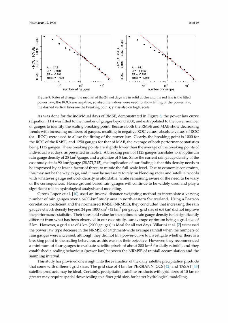
Another way to estimate the representative threshold values was to use rate of change (ROC),estimated as

ROCi =PSi+1 − PSi

PSi(Ni+1 −Ni)100 (12)

where i and i+1 are the successive number of gauges indexed when arranged in increasing order,(Ni+1 − Ni) is the difference in the number of gauges, and (PSi+1 − PSi) represents the difference inperformance statistics at the successive intervals. In comparison to RMSE and MAB, the ROC is rainfallmagnitude-independent, meaning values for the different wet days could be compared. Rates ofchange (ROC) is commonly used in finance to measure the change in the price of a security over a fixedtime interval, so the denominator (Ni+1 − Ni) is not required, or set to 1, in that sense (https://www.ambroker.com/en/analysis/blog/what-rate-change-roc-indicator-and-how-use-trading/, accessed on2 June 2020). The ROC was calculated progressively for all increasing numbers of gauges for each wetday. For a fixed number of gauges, the medians of the 24 values were selected and plotted in Figure 9.

Water 2020, 12, 1906 16 of 19

Figure 9. Rates of change: the median of the 24 wet days are in solid circles and the red line is the fittedpower law; the ROCs are negative, so absolute values were used to allow fitting of the power law;the dashed vertical lines are the breaking points; y axis also on log10 scale.

As was done for the individual days of RMSE, demonstrated in Figure 8, the power law curve(Equation (11)) was fitted to the number of gauges beyond 2000, and extrapolated to the lower numberof gauges to identify the scaling breaking point. Because both the RMSE and MAB show decreasingtrends with increasing numbers of gauges, resulting in negative ROC values, absolute values of ROC(or −ROC) were used to allow the fitting of the power law. Clearly, the breaking point is 1000 forthe ROC of the RMSE, and 1250 gauges for that of MAB, the average of both performance statisticsbeing 1125 gauges. These breaking points are slightly lower than the average of the breaking points ofindividual wet days, as presented in Table 2. A breaking point of 1125 gauges translates to an optimumrain gauge density of 25 km2/gauge, and a grid size of 5 km. Since the current rain gauge density of thecase study site is 90 km2/gauge (28,371/315), the implication of our finding is that this density needs tobe improved by at least a factor of three, to mimic the full-scale level. Due to economic constraints,this may not be the way to go, and it may be necessary to rely on blending radar and satellite recordswith whatever gauge network density is affordable, while remaining aware of the need to be waryof the consequences. Hence ground based rain gauges will continue to be widely used and play asignificant role in hydrological analysis and modelling.

Girons Lopez et al. [10] used an inverse-distance weighting method to interpolate a varyingnumber of rain gauges over a 6400-km2 study area in north-eastern Switzerland. Using a Pearsoncorrelation coefficient and the normalised RMSE (NRMSE), they concluded that increasing the raingauge network density beyond 24 per 1000 km2 (42 km2 per gauge, grid size of 6.4 km) did not improvethe performance statistics. Their threshold value for the optimum rain gauge density is not significantlydifferent from what has been observed in our case study, our average optimum being a grid size of5 km. However, a grid size of 4 km (2000 gauges) is ideal for all wet days. Villarini et al. [7] witnessedthe power law type decrease in the NRMSE of catchment-wide average rainfall when the numbers ofrain gauges were increased, although they did not fit a power-curve to investigate whether there is abreaking point in the scaling behaviour, as this was not their objective. However, they recommendeda minimum of four gauges to evaluate satellite pixels of about 200 km2 for daily rainfall, and theyestablished a scaling behaviour (power law) between the NRMSE of rainfall accumulation and thesampling interval.

This study has provided one insight into the evaluation of the daily satellite precipitation productsthat come with different grid sizes. The grid size of 4 km for PERSIANN_CCS [42] and TASAT [43]satellite products may be ideal. Certainly, precipitation satellite products with grid sizes of 10 km orgreater may require spatial downscaling to a finer grid size, for better hydrological modelling.

Water 2020, 12, 1906 17 of 19

5. Conclusions

The rain gauge continues to be a valuable source of rainfall records, despite its primary limitationof having a small coverage area, of about 203 mm in diameter, and an inadequate network density,rendering it unable to capture the high spatial variability of rainfall. For these reasons, radar andsatellite rainfall data sources are becoming popular, but can be cost-prohibitive for some areas. With theaid of bias-corrected radar daily rainfall records, this study has provided a framework for determiningthe optimum rain gauge density. The probabilities of the radar records are assumed to be correct,but the rainfall amounts were bias-corrected using observed daily rain gauge records within thestudy area. While there are many studies in the literature on the optimum rain gauge network density,there is no consensus on this. A simple practical approach is implemented to ascertain the optimumrain gauge network density.

The starting point is a unique stratified sampling technique, used to mimic the distribution ofthe current rain gauge locations that are employed to sample a fixed number of rain gauge locationsfrom the bias-corrected radar data of the wet day, with the days considered independently. This wasrepeated a number of times for a fixed number of gauges. For each set of sampled locations, the dailyrainfall amounts were transformed into normal scores that were used to develop the 2D correlogram(spatial structure) required by ordinary kriging interpolation. Then, LOOCV was carried out, and thesimulated quantiles were evaluated using the performance statistics of RMSE and MAB. Plotting theseperformance statistics against the number of rain gauges revealed a break in scaling for all the 24 wetdays analysed. Rates of change (ROC) per additional gauge of the performance statistics revealed thesame break in scaling as that depicted by RMSE and MAB. It is the breaking point in the power lawscaling that is used to infer the optimum rain gauge network density.

Generally speaking, the uncertainty concerning the median of the performance statistics decreaseswith the increasing number of gauges. This is due to the fact that the higher the number of gauges,the better the reproduction of the spatial structure of the full-scale region. The break in scaling variedbetween 750 and 2000 gauges, which translates to 38 km2/gauge (grid size ~6 km) to 14 km2/gauge(grid size ~4 km), respectively. However, no apparent reasons were established for the variations in thedaily rainfall statistics. In the end, ROC gave an average optimum network density of 25 km2/gauge,corresponding to a grid size of 5 km. Thus, the case study site’s rain gauge network density of90 km2/gauge needs to be improved by at least a factor of three in order to mimic the full-scale level.

One implication is that there may not be a real advantage in downscaling daily satellite precipitationproducts with grid sizes finer than 5 km. However, this methodology needs to be duplicated in differentregions in order to ascertain the effects of local conditions, such as orography and the spatiotemporalvariability of rainfall, on the optimum rain gauge network density. While the breaking point of thenumber of gauges varied from day to day, there were no clear linkages between this and the stormproperties, and this needs to be further investigated.

Funding: This research received no external funding.

Conflicts of Interest: The author declares no conflict of interest.

References

1. Kidd, C.; Becker, A.; Huffman, G.J.; Muller, C.L.; Joe, P.; Skofronick-Jackson, G.; Kirschbaum, D.B. So, howmuch of the Earth’s surface is covered by rain gauges? Bull. Am. Meteorol. Soc. 2017, 98, 69–78. [CrossRef]

2. Huff, F.A. Time distribution characteristics of rainfall rates. Water Resour. Res. 1970, 6, 447–454. [CrossRef]3. Yang, Z.; Hsu, K.; Sorooshian, S.; Xu, X.; Braithwaite, D.; Verbist, K.M.J. Bias adjustment of satellite-based

precipitation estimation using gauge observations: A case study in Chile. J. Geophys. Res. Atmos. 2016, 121,3790–3806. [CrossRef]

4. Germann, U.; Galli, G.; Boscacci, M.; Bolliger, M. Radar precipitation measurement in a mountainous region.Q. J. Roy. Meteorol. Soc. 2006, 132, 1669–1692. [CrossRef]

Water 2020, 12, 1906 18 of 19

5. Price, K.; Purucker, S.T.; Kraemer, S.R.; Babendreier, J.E.; Knightes, C.D. Comparison of radar and gaugeprecipitation data in watershed models across varying spatial and temporal scales. Hydrol. Process. 2013, 28,3505–3520. [CrossRef]

6. Collier, C.G. Accuracy of rainfall estimates by radar, part 1: Calibration by telemetering raingauges. J. Hydrol.1986, 83, 207–223. [CrossRef]

7. Villarini, G.; Mandapaka, P.V.; Krajewski, W.F.; Moore, R.J. Rainfall and sampling uncertainties: A rain gaugeperspective. J. Geophys. Res. 2008, 113, D11102. [CrossRef]

8. Sattari, M.-T.; Rezazadeh-Joudi, A.; Kusiak, A. Assessment of different methods for estimation of missingdata in precipitation studies. Hydrol. Res. 2017, 48, 1032–1044. [CrossRef]

9. St-Hilaire, A.; Ouarda, T.B.; Lachance, M.; Bobée, B.; Gaudet, J.; Gignac, C. Assessment of the impactof meteorological network density on the estimation of basin precipitation and runoff: A case study.Hydrol. Process. 2003, 17, 3561–3580. [CrossRef]

10. Girons Lopez, M.; Wennerström, H.; Nordén, L.Å.; Seibert, J. Location and density of rain gauges for theestimation of spatial varying precipitation. Geogr. Ann. A 2015, 97, 167–179. [CrossRef]

11. Maier, R.; Krebs, G.; Pichler, M.; Muschalla, D.; Gruber, G. Spatial Rainfall Variability in UrbanEnvironments—High-Density Precipitation Measurements on a City-Scale. Water 2020, 12, 1157. [CrossRef]

12. Faurès, J.-M.; Goodrich, D.C.; Woolhiser, D.A.; Sorooshian, S. Impact of small-scale spatial rainfall variabilityon runoff modeling. J. Hydrol. 1995, 173, 309–326. [CrossRef]

13. Bárdossy, A.; Das, T. Influence of rainfall observation network on model calibration and application.Hydrol. Earth Syst. Sci. Discuss. 2006, 3, 3691–3726. [CrossRef]

14. Mishra, A.K. Effect of Rain Gauge Density Over the Accuracy of Rainfall: A Case Study over Bangalore, India;SpringerPlus: Berlin, Germany, 2013; Volume 2, p. 311. [CrossRef]

15. Tesfagiorgis, K.; Mahani, S.E.; Krakauer, N.Y.; Khanbilvardi, R. Bias correction of satellite rainfall estimatesusing a radar-gauge product—A case study in Oklahoma (USA). Hydrol. Earth Syst. Sci. 2011, 15, 2631–2647.[CrossRef]

16. Leander, R.; Buishand, T.A. Resampling of regional climate model output for the simulation of extreme riverflows. J. Hydrol. 2007, 332, 487–496. [CrossRef]

17. Addor, N.; Seibert, J. Bias correction for hydrological impact studies-beyond the daily perspective.Hydrol. Process. 2014, 28, 4823–4828. [CrossRef]

18. Gudmundsson, L.; Bremnes, J.B.; Haugen, J.E.; Engen-Skaugen, T. Downscaling RCM precipitation to thestation scale using statistical transformations-a comparison of methods. Hydrol. Earth Syst. Sci. 2012, 16,3383–3390. [CrossRef]

19. Lafon, T.; Dadson, S.; Buys, G.; Prudhomme, C. Bias correction of daily precipitation simulated by a regionalclimate model: A comparison of methods. Int. J. Clim. 2013, 33, 1367–1381. [CrossRef]

20. Kim, K.B.; Bray, M.; Han, D. An improved bias correction scheme based on comparative precipitationcharacteristics. Hydrol. Process. 2015, 29, 2258–2266. [CrossRef]

21. Gyasi-Agyei, Y.; Pegram, G. Interpolation of daily rainfall networks using simulated radar fields for realistichydrological modelling of spatial rain field ensembles. J. Hydrol. 2014, 519, 777–791. [CrossRef]

22. Gyasi-Agyei, Y. Assessment of radar based locally varying anisotropy on daily rainfall interpolation.Hydrol. Sci. J. 2016, 61, 1890–1902. [CrossRef]

23. Gyasi-Agyei, Y. Realistic sampling of anisotropic correlogram parameters for conditional simulation of dailyrainfields. J. Hydrol. 2018, 556, 1064–1077. [CrossRef]

24. Gyasi-Agyei, Y. Propagation of uncertainties in interpolated rainfields to runoff errors. Hydrol. Sci. J. 2019,64, 587–606. [CrossRef]

25. Peel, M.C.; Finlayson, B.L.; McMahon, T.A. Updated world map of the Köppen-Geiger climate classification.Hydrol. Earth Syst. Sci. 2007, 11, 1633–1644. [CrossRef]

26. Delignette-Muller, M.L.; Dutang, C. fitdistrplus: An R package for fitting distributions. J. Stat. Softw. 2015,64, 1–34. [CrossRef]

27. Aucoin, F. FAdist: Distributions That Are Sometimes Used in Hydrology. R package version 2.3. 2020.Available online: https://CRAN.R-project.org/package=FAdist (accessed on 1 May 2020).

28. Shoji, T.; Kitaura, H. Statistical and geostatistical analysis of rainfall in central Japan. Comput. Geosci. 2006,32, 1007–1024. [CrossRef]

Water 2020, 12, 1906 19 of 19

29. Groisman, P.Y.; Karl, T.R.; Easterling, D.R.; Knight, R.W.; Jamason, P.F.; Hennessy, K.J.; Suppiah, R.; Page, C.M.;Wibig, J.; Fortuniak, K.; et al. Changes in the probability of heavy precipitation: Important indicators ofclimatic change. Clim. Chang. 1999, 42, 243–283. [CrossRef]

30. Buishand, T.A. Some remarks on the use of daily rainfall models. J. Hydrol. 1978, 36, 295–308. [CrossRef]31. Ye, L.; Hanson, L.S.; Ding, P.; Wang, D.; Vogel, R.M. The probability distribution of daily precipitation at the

point and catchment scales in the United States. Hydrol. Earth Syst. Sci. 2018, 22, 6519–6531. [CrossRef]32. Sharma, C.; Ojha, C.S.P. Changes of annual precipitation and probability distributions for different climate

types of the World. Water 2019, 11, 2092. [CrossRef]33. Yao, T.; Journel, A.G. Automatic modeling of (cross) covariance tables using fast Fourier transform. Math. Geol.

1998, 30, 589–615. [CrossRef]34. Duan, Q.; Sorooshian, S.; Gupta, V.K. Effective and efficient global optimization for conceptual rainfall-runoff

models. Water Resour. Res. 1992, 28, 1015–1031. [CrossRef]35. Cressie, N. Statistics for Spatial Data; John Wiley and Sons: New York, NY, USA, 1993.36. Ly, S.; Charles, C.; Degre, A. Geostatistical interpolation of daily rainfall at catchment scale: The use of

several variogram models in the Ourthe and Ambleve catchments, Belgium. Hydrol. Earth Syst. Sci. 2011, 15,2259–2274. [CrossRef]

37. Pebesma, E.J. Multivariable geostatistics in S: The gstat package. Comput. Geosci. 2004, 30, 683–691. [CrossRef]38. Austin, P.M. Relation between measured radar reflectivity and surface rainfall. Mon. Weather. Rev. 1987, 115,

1053–1070. [CrossRef]39. Krajewski, W.F.; Villarini, G.; Smith, J.A. Radar-rainfall uncertainties. Bull. Am. Meteorol. Soc. 2010, 91, 87–94.

[CrossRef]40. Rabiei, E.; Haberlandt, U. Applying bias correction for merging rain and radar data. J. Hydrol. 2015, 522,

544–557. [CrossRef]41. Gyasi-Agyei, Y.; de Troch, F.P.; Troch, P.A. A dynamic hillslope response model in a geomorphology based

rainfall-runoff model. J. Hydrol. 1996, 178, 1–18. [CrossRef]42. Nguyen, P.; Shearer, E.J.; Tran, H.; Ombadi, M.; Hayatbini, N.; Palacios, T.; Huynh, P.; Braithwaite, D.;

Updegraff, G.; Hsu, K.; et al. The CHRS Data Portal, an easily accessible public repository for PERSIANNglobal satellite precipitation data. Sci. Data 2019, 6, 180296. [CrossRef]

43. Maidment, R.I.; Grimes, D.; Black, E.; Tarnavsky, E.; Young, M.; Greatrex, H.; Allan, R.P.; Stein, T.H.M.;Nkonde, E.; Senkunda, S.; et al. A new, long-term daily satellite-based rainfall dataset for operationalmonitoring in Africa. Sci. Data 2017, 4, 170063. [CrossRef]

© 2020 by the author. Licensee MDPI, Basel, Switzerland. This article is an open accessarticle distributed under the terms and conditions of the Creative Commons Attribution(CC BY) license (http://creativecommons.org/licenses/by/4.0/).