rain attenuation time series synthesis with simulated rain cell
TRANSCRIPT

Ŕ periodica polytechnica
Electrical Engineering53/1-2 (2009) 11–16
doi: 10.3311/pp.ee.2009-1-2.02web: http://www.pp.bme.hu/ee
c© Periodica Polytechnica 2009
RESEARCH ARTICLE
Rain attenuation time series synthesiswith simulated rain cell movementLászló Csurgai-Horváth
Received 2008-05-10, revised 2009-01-24
AbstractThis paper proposes a stochastic modeling method to simu-
late the rain attenuation process in order to generate time seriesfor high frequency terrestrial radio links. It is also the subject ofthis research to express the local attenuation differences on con-verging radio links belonging to the same node. The simulationscene (some tenth square kilometers) is a cellular mobile radiosystem which consists of a backbone node and some millime-ter band radio links forming a star network around the node.The model parameters are extracted from the long-term mea-surement of different local meteorological parameters of an ac-tive radio network. The essentials of the model is the simulationof rain cell translation across the scene by a two dimensionalnon-symmetrical random walk (discrete time and discrete statehomogenous Markov model). A second Markov model is appliedto embed in the model the rain cell translation speed. The struc-ture of the rain cells is approximated with an elliptical model toexpress the point rainfall rate in order to calculate the path at-tenuation at discrete time steps during the simulation. The localprecipitation field allows the evaluation of the rainfall impacton the considered radio links in terms of single-link attenuationdistributions. The model is also applicable to simulate the an-nual attenuation statistics which will be compared with the realmeasurement statistics for evaluation purposes.
Keywordsrain attenuation time series · star radio-link topology ·
Markov model
AcknowledgementThis work was carried out in the framework of IST FP6 Sat-
NEx NoE project and supported by the Mobile Innovation Cen-ter, Hungary (Mobil Innovációs Központ).
László Csurgai-Horváth
Department of Broadband Infocommunications and Electromagnetic Theory,BME, H-1111 Budapest, Goldmann Gy. tér 3„ Hungarye-mail: [email protected]
1 IntroductionAfter the brief introduction of the simulation scene, the ran-
dom walk Markov model and its parameterization are described[1], [2]. It is followed by the introduction of the rain cell trans-lation speed model. Afterwards the elliptical rain cell modelwill be reviewed which is applied to express the point rainfallrate along the radio link affected by the rain cell [3–5]. In orderto simulate the long term attenuation statistics of the radio links,several rain cells have to be moved over the simulation area. Thepeak rain rate of the individual cells is weighted by the measuredannual rainfall rate statistics, allowing a realistic approximationof the rain cell distribution. Finally a simulation of multiplerain cell movement will be shown and the attenuation statisticsrelative to the radio links are calculated and compared with themeasured ones.
2 The simulation sceneThe simulation scene consists of star-structured high fre-
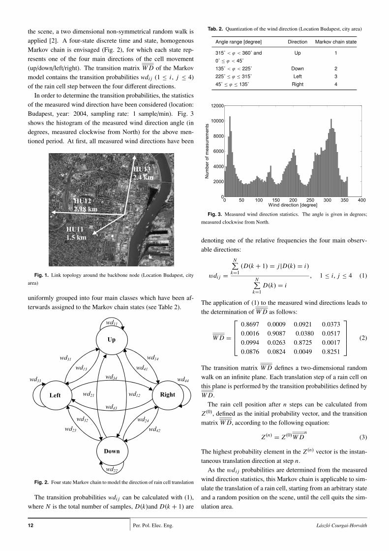
quency terrestrial radio links in a GSM network, named HU11-HU13, whose geometry is depicted in Fig. 1 and their character-istics are detailed in Table 1.
Tab. 1. Characteristics of the star-structured radio links
Link
Code
Frequency band
[GHz]
Polarization Length
[Km]
Azimuth
[deg]
HU11 38 horizontal 1.5 238
HU12 38 vertical 2.98 272
HU13 23 horizontal 2.4 10
3 Modeling the rain cell translationTo simulate the rain attenuation and generate attenuation time
series we model the meteorological environment of the radiolink area by rain cell movement simulation. To achieve our goalthe translation model of rain cells simulates the direction andspeed of their movement. At first the moving direction modelwill be introduced, followed by the description of the translationspeed simulation.
In order to model the translation direction of the rain cells on
Rain attenuation time series synthesis with simulated rain cell movement 112009 53 1-2
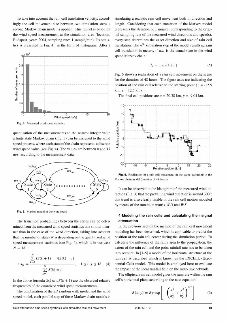
the scene, a two dimensional non-symmetrical random walk isapplied [2]. A four-state discrete time and state, homogenousMarkov chain is envisaged (Fig. 2), for which each state rep-resents one of the four main directions of the cell movement(up/down/left/right). The transition matrix W D of the Markovmodel contains the transition probabilities wdi j (1 ≤ i , j ≤ 4)of the rain cell step between the four different directions.
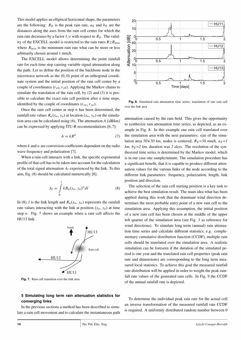
In order to determine the transition probabilities, the statisticsof the measured wind direction have been considered (location:Budapest, year: 2004, sampling rate: 1 sample/min). Fig. 3shows the histogram of the measured wind direction angle (indegrees, measured clockwise from North) for the above men-tioned period. At first, all measured wind directions have been
2
Figure 1. Link topology around the backbone node
(Location Budapest, city area)
Modeling the rain cell translation
To simulate the rain attenuation and generate attenuation time series we model the meteorological environment of the radio
link area by rain cell movement simulation. To achieve our goal the translation model of rain cells simulates the direction and
speed of their movement. At first the moving direction model will be introduced, followed by the description of the translation
speed simulation.
In order to model the translation direction of the rain cells on the scene, a two dimensional non-symmetrical random walk is
applied [2]. A four-state discrete time and state, homogenous Markov chain is envisaged (Figure 2.), for which each state
represents one of the four main directions of the cell movement (up/down/left/right). The transition matrix WD of the Markov
model contains the transition probabilities wdij (1 ≤ i, j ≤ 4) of the rain cell step between the four different directions.
Figure 2. Four state Markov chain to model the direction of rain cell translation
In order to determine the transition probabilities, the statistics of the measured wind direction have been considered (location:
Budapest, year: 2004, sampling rate: 1 sample/min). Figure 3. shows the histogram of the measured wind direction angle (in
degrees, measured clockwise from North) for the above mentioned period.
HU13
2.4 km
HU11
1.5 km
HU12
2.98 km
Up
Down
Left Right
wd11
wd22
wd33 wd44
wd12
wd14
wd41
wd31
wd13
wd23
wd32 wd24
wd42
wd34
wd43
wd21
Fig. 1. Link topology around the backbone node (Location Budapest, cityarea)
uniformly grouped into four main classes which have been af-terwards assigned to the Markov chain states (see Table 2).
2
Figure 1. Link topology around the backbone node
(Location Budapest, city area)
Modeling the rain cell translation
To simulate the rain attenuation and generate attenuation time series we model the meteorological environment of the radio
link area by rain cell movement simulation. To achieve our goal the translation model of rain cells simulates the direction and
speed of their movement. At first the moving direction model will be introduced, followed by the description of the translation
speed simulation.
In order to model the translation direction of the rain cells on the scene, a two dimensional non-symmetrical random walk is
applied [2]. A four-state discrete time and state, homogenous Markov chain is envisaged (Figure 2.), for which each state
represents one of the four main directions of the cell movement (up/down/left/right). The transition matrix WD of the Markov
model contains the transition probabilities wdij (1 ≤ i, j ≤ 4) of the rain cell step between the four different directions.
Figure 2. Four state Markov chain to model the direction of rain cell translation
In order to determine the transition probabilities, the statistics of the measured wind direction have been considered (location:
Budapest, year: 2004, sampling rate: 1 sample/min). Figure 3. shows the histogram of the measured wind direction angle (in
degrees, measured clockwise from North) for the above mentioned period.
HU13
2.4 km
HU11
1.5 km
HU12
2.98 km
Up
Down
Left Right
wd11
wd22
wd33 wd44
wd12
wd14
wd41
wd31
wd13
wd23
wd32 wd24
wd42
wd34
wd43
wd21
Fig. 2. Four state Markov chain to model the direction of rain cell translation
The transition probabilities wdi j can be calculated with (1),where N is the total number of samples, D(k)and D(k + 1) are
Tab. 2. Quantization of the wind direction (Location Budapest, city area)
Angle range [degree] Direction Markov chain state
315˚ < ϕ < 360˚ and
0˚ ≤ ϕ < 45˚
Up 1
135˚ < ϕ < 225˚ Down 2
225˚ ≤ ϕ ≤ 315˚ Left 3
45˚ ≤ ϕ ≤ 135˚ Right 4
3
0 50 100 150 200 250 300 350 4000
2000
4000
6000
8000
10000
12000
Number of measurements
Wind direction [degree]
Figure 3. Measured wind direction statistics. The angle is given in degrees; measured clockwise from North.
At first, all measured wind directions have been uniformly grouped into four main classes which have been afterwards
assigned to the Markov chain states (see Table 2.).
Table 2: Quantization of the wind direction
Angle range [degree] Direction Markov chain state
315° < ϕ < 360° and 0° ≤ ϕ < 45°
Up 1
135° < ϕ < 225° Down 2
225° ≤ ϕ ≤ 315° Left 3
45° ≤ ϕ ≤ 135° Right 4
The transition probabilities wdij can be calculated with (1), where N is the total number of samples, D(k) and D(k+1) are
denoting one of the relative frequencies the four main observable directions:
∑∑∑∑
∑∑∑∑
====
====
====
========++++====
N
k
N
kij
ikD
ikDjkD
wd
1
1
)(
))(|)1((
, 1 ≤ i, j ≤ 4 (1)
The application of (1) to the measured wind directions leads to the determination of WD as it follows:
====
0.82510.00490.08240.0876
0.00170.87250.02630.0994
0.05170.03800.90870.0016
0.03730.09210.00090.8697
WD (2)
The transition matrix WD defines a two-dimensional random walk on an infinite plane. Each translation step of a rain cell on
this plane is performed by the transition probabilities defined by WD .
The rain cell position after n steps can be calculated from Z(0), defined as the initial probability vector, and the transition matrix
WD , according to the following equation:
n
n WDZZ )0()( ==== (3)
The highest probability element in the Z(n) vector is the instantaneous translation direction at step n.
Fig. 3. Measured wind direction statistics. The angle is given in degrees;measured clockwise from North.
denoting one of the relative frequencies the four main observ-able directions:
wdi j =
N∑k=1
(D(k + 1) = j |D(k) = i)
N∑k=1
D(k) = i, 1 ≤ i, j ≤ 4 (1)
The application of (1) to the measured wind directions leads tothe determination of W D as follows:
W D =
0.8697 0.0009 0.0921 0.03730.0016 0.9087 0.0380 0.05170.0994 0.0263 0.8725 0.00170.0876 0.0824 0.0049 0.8251
(2)
The transition matrix W D defines a two-dimensional randomwalk on an infinite plane. Each translation step of a rain cell onthis plane is performed by the transition probabilities defined byW D.
The rain cell position after n steps can be calculated fromZ (0), defined as the initial probability vector, and the transitionmatrix W D, according to the following equation:
Z (n)= Z (0)W D
n(3)
The highest probability element in the Z (n) vector is the instan-taneous translation direction at step n.
As the wd i j probabilities are determined from the measuredwind direction statistics, this Markov chain is applicable to sim-ulate the translation of a rain cell, starting from an arbitrary stateand a random position on the scene, until the cell quits the sim-ulation area.
Per. Pol. Elec. Eng.12 László Csurgai-Horváth
To take into account the rain cell translation velocity, accord-ingly the cell movement size between two simulation steps asecond Markov chain model is applied. This model is based onthe wind speed measurement at the simulation area (location:Budapest, year: 2004, sampling rate: 1 sample/min). Its statis-tics is presented in Fig. 4. in the form of histogram. After a
4
As the wdij probabilities are determined from the measured wind direction statistics, this Markov chain is applicable to
simulate the translation of a rain cell, starting from an arbitrary state and a random position on the scene, until the cell quits the
simulation area.
To take into account the rain cell translation velocity, accordingly the cell movement size between two simulation steps a
second Markov chain model is applied. This model is based on the wind speed measurement at the simulation area (location:
Budapest, year: 2004, sampling rate: 1 sample/min). Its statistics is presented in Figure 4. in the form of histogram.
0 5 10 15 200
0.5
1
1.5
2
2.5
3x 10
5
Number of measurements
Wind speed [m/s]
Figure 4. Measured wind speed statistics.
After a quantization of the measurements to the nearest integer value a finite state Markov chain (Figure 5.) can be assigned to
the wind speed process, where each state of the chain represents a discrete wind speed value (see Figure 4.). The values are
between 0 and 17 m/s, according to the measurement data.
Figure 5. Markov model of the wind speed
The transition probabilities between the states can be determined from the measured wind speed statistics in a similar manner
than in the case of the wind direction, taking into account that the number of states N is depending on the quantized wind speed
measurement statistics (see Figure 4.), which is in our case N=18.
∑∑∑∑
∑∑∑∑
====
====
====
========++++====
N
k
N
kij
ikS
ikSjkS
ws
1
1
)(
))(|)1((
, 1 ≤ i, j ≤ 18 (4)
In the above formula S(k) and S(k+1) are the observed relative frequencies of the quantized wind speed measurements.
The combination of the 2D random walk model and the wind speed model, each parallel step of these Markov chain models is
simulating a realistic rain cell movement both in direction and length. Considering that each transition of the Markov model
State
1
wsN1
wsN2
ws2N
State
2
ws22
ws1N
ws11 State
N
ws21
ws12
wsNN
Fig. 4. Measured wind speed statistics
quantization of the measurements to the nearest integer valuea finite state Markov chain (Fig. 5) can be assigned to the windspeed process, where each state of the chain represents a discretewind speed value (see Fig. 4). The values are between 0 and 17m/s, according to the measurement data.
4
As the wdij probabilities are determined from the measured wind direction statistics, this Markov chain is applicable to
simulate the translation of a rain cell, starting from an arbitrary state and a random position on the scene, until the cell quits the
simulation area.
To take into account the rain cell translation velocity, accordingly the cell movement size between two simulation steps a
second Markov chain model is applied. This model is based on the wind speed measurement at the simulation area (location:
Budapest, year: 2004, sampling rate: 1 sample/min). Its statistics is presented in Figure 4. in the form of histogram.
0 5 10 15 200
0.5
1
1.5
2
2.5
3x 10
5
Number of measurements
Wind speed [m/s]
Figure 4. Measured wind speed statistics.
After a quantization of the measurements to the nearest integer value a finite state Markov chain (Figure 5.) can be assigned to
the wind speed process, where each state of the chain represents a discrete wind speed value (see Figure 4.). The values are
between 0 and 17 m/s, according to the measurement data.
Figure 5. Markov model of the wind speed
The transition probabilities between the states can be determined from the measured wind speed statistics in a similar manner
than in the case of the wind direction, taking into account that the number of states N is depending on the quantized wind speed
measurement statistics (see Figure 4.), which is in our case N=18.
∑∑∑∑
∑∑∑∑
====
====
====
========++++====
N
k
N
kij
ikS
ikSjkS
ws
1
1
)(
))(|)1((
, 1 ≤ i, j ≤ 18 (4)
In the above formula S(k) and S(k+1) are the observed relative frequencies of the quantized wind speed measurements.
The combination of the 2D random walk model and the wind speed model, each parallel step of these Markov chain models is
simulating a realistic rain cell movement both in direction and length. Considering that each transition of the Markov model
State
1
wsN1
wsN2
ws2N
State
2
ws22
ws1N
ws11 State
N
ws21
ws12
wsNN
Fig. 5. Markov model of the wind speed
The transition probabilities between the states can be deter-mined from the measured wind speed statistics in a similar man-ner than in the case of the wind direction, taking into accountthat the number of states N is depending on the quantitized windspeed measurement statistics (see Fig. 4), which is in our caseN = 18.
wsi j =
N∑k=1
(S(k + 1) = j |S(k) = i)
N∑k=1
S(k) = i, 1 ≤ i, j ≤ 18 (4)
In the above formula S(k)andS(k + 1) are the observed relativefrequencies of the quantized wind speed measurements.
The combination of the 2D random walk model and the windspeed model, each parallel step of these Markov chain models is
simulating a realistic rain cell movement both in direction andlength. Considering that each transition of the Markov modelrepresents the duration of 1 minute (corresponding to the origi-nal sampling rate of the measured wind directions and speeds),every step determines the exact direction and size of rain celltranslation. The nth simulation step of the model results dn raincell translation in meters, if wsn is the actual state in the windspeed Markov chain:
dn = wsn/60 [m] (5)
Fig. 6 shows a realization of a rain cell movement on the scenefor the duration of 48 hours. The figure axes are indicating theposition of the rain cell relative to the starting point (x = -12.5km, y = 12.5 km).
The final cell positions are x = 20.38 km, y = -9.04 km.
5
represents the duration of 1 minute (corresponding to the original sampling rate of the measured wind directions and speeds),
every step determines the exact direction and size of rain cell translation. The nth simulation step of the model results dn rain
cell translation in meters, if wsn is the actual state in the wind speed Markov chain:
][60/ mwsd nn ==== (5)
Figure 6.Figure shows a realization of a rain cell movement on the scene for the duration of 48 hours. The figure axes are
indicating the position of the rain cell relative to the starting point (x = -12.5 km, y = 12.5 km).
The final cell positions are x = 20.38 km, y = -9.04 km.
-15 -10 -5 0 5 10 15 20 25-20
-15
-10
-5
0
5
10
15
Relative position [km]
Relative position [km]
Figure 6. Realization of a rain cell movement on the scene according to the Markov chain model (duration of 48 hours)
It can be observed in the histogram of the measured wind direction (Figure 3.Figure ) that the prevailing wind direction is
around 300°: this trend is also clearly visible in the rain cell motion modeled by means of the transition matrix WD and WS .
Modeling the rain cells and calculating their signal attenuation
In the previous section the method of the rain cell movement modeling has been described, which is applicable to predict the
position of the rain cell center during the simulation period. To calculate the influence of the rainy area to the propagation, the
extent of the rain cell and the point rainfall rate has to be taken into account. In [3, 4, 5] a model of the horizontal structure of
the rain cell is described which is known as the EXCELL (Exponential Cell) model. This model is employed here to evaluate
the impact of the local rainfall field on the radio link network.
The elliptical rain cell model gives the rain rate within the rain cell’s horizontal plane according to the next equation:
++++−−−−====
2/1
2
2
2
2
exp),(EE
Eb
y
a
xRyxR (6)
This model applies an elliptical horizontal shape, the parameters are the following: RE is the peak rain rate, aE and bE are the
distances along the axes from the rain cell center for which the rain rate decreases by a factor 1/e with respect to RE. The
validity of the EXCELL model is restricted to the rain rates R≥Rmin where Rmin is the minimum rain rate what can be more or
less arbitrarily chosen around 1 mm/h.
The EXCELL model allows determining the point rainfall rate for each time step causing variable signal attenuation along the
path. Let us define the position of the backbone node in the microwave network as the (0, 0) point of an orthogonal coordinate
system and the initial position of the rain cell center by a couple of coordinates (rx0, ry0). Applying the Markov chains to
simulate the translation of the rain cell, by (3) and (5) is possible to calculate the exact rain cell position after n time steps,
identified by the couple of coordinates (rxn, ryn).
Once the rain cell center at step n has been determined, the rainfall rate values Rn(xn, yn) at location (xn, yn) on the simulation
area can be calculated using (6). The attenuation A [dB/km] can be expressed by applying ITU-R recommendations [6] and [7]:
Fig. 6. Realization of a rain cell movement on the scene according to theMarkov chain model (duration of 48 hours)
It can be observed in the histogram of the measured wind di-rection (Fig. 3) that the prevailing wind direction is around 300˚:this trend is also clearly visible in the rain cell motion modeledby means of the transition matrix W D and W S.
4 Modeling the rain cells and calculating their signalattenuationIn the previous section the method of the rain cell movement
modeling has been described, which is applicable to predict theposition of the rain cell center during the simulation period. Tocalculate the influence of the rainy area to the propagation, theextent of the rain cell and the point rainfall rate has to be takeninto account. In [3–5] a model of the horizontal structure of therain cell is described which is known as the EXCELL (Expo-nential Cell) model. This model is employed here to evaluatethe impact of the local rainfall field on the radio link network.
The elliptical rain cell model gives the rain rate within the raincell’s horizontal plane according to the next equation:
R(x, y) = RE exp
−
(x2
a2E
+y2
b2E
)1/2 (6)
Rain attenuation time series synthesis with simulated rain cell movement 132009 53 1-2
This model applies an elliptical horizontal shape, the parametersare the following: RE is the peak rain rate, aE and bE are thedistances along the axes from the rain cell center for which therain rate decreases by a factor 1/e with respect to RE . The valid-ity of the EXCELL model is restricted to the rain rates R≥Rmin
where Rmin is the minimum rain rate what can be more or lessarbitrarily chosen around 1 mm/h.
The EXCELL model allows determining the point rainfallrate for each time step causing variable signal attenuation alongthe path. Let us define the position of the backbone node in themicrowave network as the (0, 0) point of an orthogonal coordi-nate system and the initial position of the rain cell center by acouple of coordinates (rx0, ry0). Applying the Markov chains tosimulate the translation of the rain cell, by (2) and (3) it is pos-sible to calculate the exact rain cell position after n time steps,identified by the couple of coordinates (rxn, ryn).
Once the rain cell center at step n has been determined, therainfall rate values Rn(xn, yn) at location (xn, yn) on the simula-tion area can be calculated using (6). The attenuation A [dB/km]can be expressed by applying ITU-R recommendations [6, 7]:
A = k Rα (7)
where k and α are conversion coefficients dependent on the radiowave frequency and polarization [7].
When a rain cell interacts with a link, the specific exponentialprofile of that cell has to be taken into account for the calculationof the total signal attenuation Al experienced by the link. To thisaim, Eq. (8) should be calculated numerically [8].
Al =
l∫0
k Rn(xn, yn)αdl (8)
In (8), l is the link length and Rn(xn , yn) represents the rainfallrate values interacting with the link at position (xn, yn) at timestep n. Fig. 7 shows an example when a rain cell affects theHU13 link.
6
αkRA = (7)
where k and α are conversion coefficients dependent on the radio wave frequency and polarization [7]. When a rain cell interacts with a link, the specific exponential profile of that cell has to be taken into account for the
calculation of the total signal attenuation Al experienced by the link. To this aim, equation (8) should be calculated numerically
[8].
dlyxkRA
l
nnnl ∫=0
),( α (8)
In (8), l is the link length and Rn(xn, yn) represents the rainfall rate values interacting with the link at position (xn, yn) at time
step n. Figure 7.Figure shows an example when a rain cell affects the HU13 link.
Figure 7. Rain cell transition over the link area
Simulating long term rain attenuation statistics for converging links
In the previous sections a method has been described to simulate a rain cell movement and to calculate the instantaneous path
attenuation caused by the rain field. This gives the opportunity to synthesize rain attenuation time series, as depicted, as an
example in Figure 8. In this example one rain cell translated over the simulation area with the next parameters: size of the
simulation area 50*50 km, nodes is centered, RE=50 mm/h, aE=1 km, bE=2 km, duration was 2 days. The resolution of the
synthesized time series is determined by the Markov model, which is in our case one sample/minute. The simulation procedure
has a significant benefit, that it is capable to produce different attenuation values for the various links of the node according to
the different link parameters: frequency, polarization, length, link position and direction.
0 0.5 1 1.5 20
10
20
HU11
0 0.5 1 1.5 20
20
40
Attenuation [dB]
HU12
0 0.5 1 1.5 20
5
10
Time [days]
HU13
Figure 8. Simulated rain attenuation time series; translation of one rain cell over the link area
The selection of the rain cell starting position is a key task to achieve the best simulation result. The main idea what has been
applied during this work that the dominant wind direction determines the most probable entry point of a new rain cell to the
simulation area. Applying this assumption, the initial position of a new rain cell has been chosen at the middle of the upper left
quarter of the simulation area (see Figure 3. as reference for wind directions). To simulate long term (annual) rain attenuation
HU13
HU11
HU12
North
Rain cell
Fig. 7. Rain cell transition over the link area
5 Simulating long term rain attenuation statistics forconverging linksIn the previous sections a method has been described to simu-
late a rain cell movement and to calculate the instantaneous path
6
αkRA = (7)
where k and α are conversion coefficients dependent on the radio wave frequency and polarization [7]. When a rain cell interacts with a link, the specific exponential profile of that cell has to be taken into account for the
calculation of the total signal attenuation Al experienced by the link. To this aim, equation (8) should be calculated numerically
[8].
dlyxkRA
l
nnnl ∫=0
),( α (8)
In (8), l is the link length and Rn(xn, yn) represents the rainfall rate values interacting with the link at position (xn, yn) at time
step n. Figure 7.Figure shows an example when a rain cell affects the HU13 link.
Figure 7. Rain cell transition over the link area
Simulating long term rain attenuation statistics for converging links
In the previous sections a method has been described to simulate a rain cell movement and to calculate the instantaneous path
attenuation caused by the rain field. This gives the opportunity to synthesize rain attenuation time series, as depicted, as an
example in Figure 8. In this example one rain cell translated over the simulation area with the next parameters: size of the
simulation area 50*50 km, nodes is centered, RE=50 mm/h, aE=1 km, bE=2 km, duration was 2 days. The resolution of the
synthesized time series is determined by the Markov model, which is in our case one sample/minute. The simulation procedure
has a significant benefit, that it is capable to produce different attenuation values for the various links of the node according to
the different link parameters: frequency, polarization, length, link position and direction.
0 0.5 1 1.5 20
10
20
HU11
0 0.5 1 1.5 20
20
40
Attenuation [dB]
HU12
0 0.5 1 1.5 20
5
10
Time [days]
HU13
Figure 8. Simulated rain attenuation time series; translation of one rain cell over the link area
The selection of the rain cell starting position is a key task to achieve the best simulation result. The main idea what has been
applied during this work that the dominant wind direction determines the most probable entry point of a new rain cell to the
simulation area. Applying this assumption, the initial position of a new rain cell has been chosen at the middle of the upper left
quarter of the simulation area (see Figure 3. as reference for wind directions). To simulate long term (annual) rain attenuation
HU13
HU11
HU12
North
Rain cell
Fig. 8. Simulated rain attenuation time series; translation of one rain cellover the link area
attenuation caused by the rain field. This gives the opportunityto synthesize rain attenuation time series, as depicted, as an ex-ample in Fig. 8. In this example one rain cell translated overthe simulation area with the next parameters: size of the simu-lation area 50×50 km, nodes is centered, RE=50 mm/h, aE=1km, bE=2 km, duration was 2 days. The resolution of the syn-thesized time series is determined by the Markov model, whichis in our case one sample/minute. The simulation procedure hasa significant benefit, that it is capable to produce different atten-uation values for the various links of the node according to thedifferent link parameters: frequency, polarization, length, linkposition and direction.
The selection of the rain cell starting position is a key task toachieve the best simulation result. The main idea what has beenapplied during this work that the dominant wind direction de-termines the most probable entry point of a new rain cell to thesimulation area. Applying this assumption, the initial positionof a new rain cell has been chosen at the middle of the upperleft quarter of the simulation area (see Fig. 3 as reference forwind directions). To simulate long term (annual) rain attenua-tion time series and calculate different statistics, e.g. comple-mentary cumulative distribution function (CCDF), multiple raincells should be translated over the simulation area. A realisticsimulation can be foreseen if the duration of the simulated pe-riod is one year and the translated rain cell properties (peak rainrate and dimensions) are corresponding to the long term mea-sured local statistics. To achieve this goal the measured rainfallrate distribution will be applied in order to weight the peak rain-fall rate values of the generated rain cells. In Fig. 9 the CCDFof the annual rainfall rate is depicted.
To determine the individual peak rain rate for the actual cellan inverse transformation of the measured rainfall rate CCDFis required. A uniformly distributed random number between 0
Per. Pol. Elec. Eng.14 László Csurgai-Horváth

Fig. 9. Annual rainfall rate CCDF; measured in2004 and the peak rainfall rate selection method
7
time series and calculate different statistics, e.g. complementary cumulative distribution function (CCDF), multiple rain cells
should be translated over the simulation area. A realistic simulation can be foreseen if the duration of the simulated period is
one year and the translated rain cell properties (peak rain rate and dimensions) are corresponding to the long term measured
local statistics. To achieve this goal the measured rainfall rate distribution will be applied in order to weight the peak rainfall
rate values of the generated rain cells. In Figure 9. the CCDF of the annual rainfall rate is depicted.
0 50 100 150
10-4
10-2
100
Rain rate [mm/h]
Probability
Figure 9. Annual rainfall rate CCDF; measured in 2004 and the peak rainfall rate selection method
To determine the individual peak rain rate for the actual cell an inverse transformation of the measured rainfall rate CCDF is
required. A uniformly distributed random number between 0 and 1 is generated to select the actual peak rainfall rate
probability. The corresponding rain intensity can be read from the vertical axis of the CCDF and this value will be applied as
the peak rain rate in the EXCELL model. The process is graphed in Figure 9.
Further parameters of the rain cell are the aE and bE extents. Their values can be also specified according to the average rain
cell dimensions based on local measurements. According to [9], during the simulation the rain cell extents are randomized
between 0-2 km. The next enumeration summarizes the parameters applied for the annual rain attenuation CCDF simulation:
- Simulation area: 50x50 km2; the location of HU11-13 links node is the center of the scene
- Duration of the simulation: 365 days
- Rain cell moving direction and speed are controlled by Markov chains
- Peak rain rate value RM : randomly selected by inverse transformation of the measured rain rate CCDF
- Equivalent rain cell radius aE and bE: randomized between 0-2 km
- Rain cells initial position: middle of the upper left quarter of the simulation area
- Individual movement duration: 48 hours (an adequate time interval to cross the cell the whole scene)
- 5 annual simulation runs are averaged
The result of the simulation is depicted in Figure 10.:
0 10 20 30 40 5010
-8
10-6
10-4
10-2
100
Attenuation [dB]
Probability
HU11 Simulated
HU11 Measured
HU12 Simulated
HU12 Measured
HU13 Simulated
HU13 Measured
Figure 10. Simulated and measured rain attenuation CCDFs
Random
number
Instantaneous peak rain rate
and 1 is generated to select the actual peak rainfall rate prob-ability. The corresponding rain intensity can be read from thevertical axis of the CCDF and this value will be applied as thepeak rain rate in the EXCELL model. The process is graphed inFig. 9.
Further parameters of the rain cell are the aE and bE extents.Their values can be also specified according to the average raincell dimensions based on local measurements. According to [9],during the simulation the rain cell extents are randomized be-tween 0-2 km. The next enumeration summarizes the parame-ters applied for the annual rain attenuation CCDF simulation:
• Simulation area: 50x50 km2; the location of HU11-13 linksnode is the center of the scene
• Duration of the simulation: 365 days
• Rain cell moving direction and speed are controlled byMarkov chains
• Peak rain rate value RM : randomly selected by inverse trans-formation of the measured rain rate CCDF
• Equivalent rain cell radius aE and bE : randomized between0-2 km
• Rain cells initial position: middle of the upper left quarter ofthe simulation area
• Individual movement duration: 48 hours (an adequate timeinterval to cross the cell the whole scene)
• 5 annual simulation runs are averaged
The result of the simulation is depicted in Fig. 10:The measured CCDF of rain attenuation is compared with the
simulated CCDFs for the investigated links HU11, HU12 andHU13. It is very well observable that the model approximateswith low deviation the measured statistics. The local differencesdue to the variant link parameters are also correctly simulated.
7
time series and calculate different statistics, e.g. complementary cumulative distribution function (CCDF), multiple rain cells
should be translated over the simulation area. A realistic simulation can be foreseen if the duration of the simulated period is
one year and the translated rain cell properties (peak rain rate and dimensions) are corresponding to the long term measured
local statistics. To achieve this goal the measured rainfall rate distribution will be applied in order to weight the peak rainfall
rate values of the generated rain cells. In Figure 9. the CCDF of the annual rainfall rate is depicted.
0 50 100 150
10-4
10-2
100
Rain rate [mm/h]
Probability
Figure 9. Annual rainfall rate CCDF; measured in 2004 and the peak rainfall rate selection method
To determine the individual peak rain rate for the actual cell an inverse transformation of the measured rainfall rate CCDF is
required. A uniformly distributed random number between 0 and 1 is generated to select the actual peak rainfall rate
probability. The corresponding rain intensity can be read from the vertical axis of the CCDF and this value will be applied as
the peak rain rate in the EXCELL model. The process is graphed in Figure 9.
Further parameters of the rain cell are the aE and bE extents. Their values can be also specified according to the average rain
cell dimensions based on local measurements. According to [9], during the simulation the rain cell extents are randomized
between 0-2 km. The next enumeration summarizes the parameters applied for the annual rain attenuation CCDF simulation:
- Simulation area: 50x50 km2; the location of HU11-13 links node is the center of the scene
- Duration of the simulation: 365 days
- Rain cell moving direction and speed are controlled by Markov chains
- Peak rain rate value RM : randomly selected by inverse transformation of the measured rain rate CCDF
- Equivalent rain cell radius aE and bE: randomized between 0-2 km
- Rain cells initial position: middle of the upper left quarter of the simulation area
- Individual movement duration: 48 hours (an adequate time interval to cross the cell the whole scene)
- 5 annual simulation runs are averaged
The result of the simulation is depicted in Figure 10.:
0 10 20 30 40 5010
-8
10-6
10-4
10-2
100
Attenuation [dB]
Probability
HU11 Simulated
HU11 Measured
HU12 Simulated
HU12 Measured
HU13 Simulated
HU13 Measured
Figure 10. Simulated and measured rain attenuation CCDFs
Random
number
Instantaneous peak rain rate
Fig. 10. Simulated and measured rain attenuation CCDFs
6 ConclusionIn this paper a Markov chain based stochastic model for the
simulation of rain cells translation has been introduced and usedto generate rain attenuation time series for converging terrestrialradio links. The method is also applicable to simulate the longterm rain attenuation statistics. The cell movement model is pa-rameterized from local wind direction and speed measurements.Several rain cells are translated over to simulation area to get theannual attenuation statistics. The impact of the individual raincells are weighted by the measured local rainfall rate distribu-tion. The rain cell profile has been modeled with the EXCELLmethod, which is applicable to express the point rainfall rate andin this way the instantaneous path attenuation can be calculated.
The simulation results have quite good correlation with themeasured annual attenuation statistics relative to the individuallinks. The future work can be also focused on the investigationof the dynamic parameters of the synthesized time series e.g.fade and interfade duration and fade slope statistics.
Rain attenuation time series synthesis with simulated rain cell movement 152009 53 1-2
References1 Papoulis A, Probability, Random Variables and Stochastic Processes,
McGraw-Hill, New York, 2001. 3rd edition.2 Csurgai-Horváth L, Bitó J, Spatial Markov Model of Fade Duration on
Terrestrial Radio Links, 2nd European Conference on Antennas and Propaga-tion: EuCAP 2007 (Edinburgh, England, 2007), DOI 10.1049/ic.2007.0873,(to appear in print).
3 Capsoni C, Fedi F, Magistroni C, Paraboni A, Pawlina A, Data
and theory for a new model of the horizontal structure of rain cells for
propagation applications, Radio Science 22 (1987), no. 3, 395-404, DOI10.1029/RS022i003p00395.
4 Capsoni C, Fedi F, Paraboni A, A comprehensive meteorologically ori-
ented methodology for the prediction of wave propagation parameters in
telecommunication applications beyond 10 GHz, Radio Science 22 (1987),no. 3, 387-393, DOI 10.1029/RS022i003p00387.
5 Riva C, Matricciani E, Luini L, Irizar M, Lacoste F, Castanet L, Charac-
terisation and modelling of rain attenuation in 20-50 GHz band, ESA work-shop on Earthspace propagation (Noordwijk, Netherlands, November 2005).
6 Propagation data and prediction methods required for the design of terres-
trial line-of-sight systems, 2001.7 Specific attenuation model for rain for use in prediction methods, 2003.8 Sinka Cs, Bitó J, Site Diversity against Rain Fading in LMDS Systems, Spe-
cial Issue of IEEE Microwave and Wireless Components Letters 13 (August2003), no. 8, 317-319, DOI 10.1109/LMWC.2003.815702.
9 Laurent Castanet (ed.), Influence of the Variability of the Propagation
Channel on Mobile, Fixed Multimedia and Optical Satellite Communica-
tions, Shaker, 2008.
Per. Pol. Elec. Eng.16 László Csurgai-Horváth