arX

iv:c

ond-

mat

/030

1152

v1 [

cond

-mat

.sta

t-m

ech]

10

Jan

2003

Charite, Biochemistry 03/01

Hydrodynamics and transport coefficients for Granular Gases

Nikolai Brilliantov1,2, Thorsten Poschel11Institut fur Biochemie, Charite, Monbijoustraße 2, 10117 Berlin, Germany

2Moscow State University, 119899 Moscow, Russia

(Dated: February 23, 2009)

The hydrodynamics of granular gases of viscoelastic particles, whose collision is described byan impact-velocity dependent coefficient of restitution, is developed using a modified Chapman-Enskog approach. We derive the hydrodynamic equations and the according transport coefficientswith the assumption that the shape of the velocity distribution function follows adiabatically thedecaying temperature. We show numerically that this approximation is justified up to intermediatedissipation. The transport coefficients and the coefficient of cooling are expressed in terms ofthe elastic and dissipative parameters of the particle material and by the gas parameters. Thedependence of these coefficients on temperature differs qualitatively from that obtained with thesimplifying assumption of a constant coefficient of restitution which was used in previous studies.The approach formulated for gases of viscoelastic particles may be applied also for other impact-velocity dependencies of the restitution coefficient.

PACS numbers: 81.05.Rm, 47.10.+g, 05.20.Dd, 51.10.+y

I. INTRODUCTION

Granular systems composed of a large number of dis-sipatively interacting particles behave in many respectsas a continuous medium and may be, in principle, de-scribed by a set of hydrodynamic equations with appro-priate boundary conditions. Although this approach issuccessively used in various fields of engineering and soilmechanics (e.g. [1, 2]) a first-principle theory for densegranular media is still lacking. Hydrodynamics may bealso applied to much simpler systems, such as rarefiedgranular gases. It has been used to describe many differ-ent processes, e.g. rapid granular flows, structure forma-tion, etc. (see [3] for an overview). For these systems thehydrodynamic equations are not postulated but derivedfrom the Boltzmann equation. The corresponding trans-port coefficients are not phenomenological constants, in-stead they are obtained by regular methods, such as theGrad method [4] or the Chapman-Enskog method [5].In most of the studies, which address the derivation ofhydrodynamic equations and kinetic coefficients, it wasassumed that the coefficient of restitution ε is a materialconstant, e.g. [6, 7, 8, 9, 10, 11, 12, 13].

This assumption simplifies the analysis enormously,however, it is neither in agreement with experimentalobservations (e.g. [14, 15, 16]) nor with basic mechanicsof particle collisions [17]. The coefficient of restitutiondepends on the impact velocity g and tends to unity forvery small g. As a consequence, particles behave moreand more elastically as the average velocity of the grainsdecreases. The simplest collision model which accountsfor dissipative material deformation, is the model of vis-coelastic particles. It is assumed in this model that theelastic stress in the bulk of the particle material dependslinearly on the strain, whereas the dissipative stress de-pends linearly on the strain rate.

Based on the fundamental work by Hertz [18] the in-teraction force between colliding viscoelastic spheres has

been derived [19]. Using this generalized Hertz law thecoefficient of restitution of viscoelastic particles can begiven as a function of the impact velocity and materialparameters [20]:

ε = 1 − C1Aα2/5g1/5 +

3

5C2

1A2α4/5g2/5 ∓ . . . (1)

with

g ≡ |~e · (~v1 − ~v2)| = |~e · ~v12| . (2)

The unit vector ~e = ~r12/r12 specifies the collision geome-try, i.e., the relative position ~r12 = ~r1−~r2 of the particlesat the collision instant. Their pre-collision velocities aregiven by ~v1 and ~v2. The elastic constant

α =

(

3

2

)3/2Y√R eff

meff (1 − ν2), (3)

depends on the effective mass and radius meff ≡m1m2/(m1+m2), R

eff ≡ R1R2/(R1+R2) of the collidingspheres, on the Young modulus Y , and on the Poissonratio ν of the particle material. The dissipative coeffi-cient A is a function of dissipative and elastic constants(see [19] for details). Finally, C1 is a numerical constant[17, 20]:

C1 =

√π

21/552/5

Γ (3/5)

Γ (21/10)≈ 1.15344 . (4)

Equation (1) describes pure viscoelastic interaction. Theassumption of viscoelastic deformation is justified if theimpact velocity is not too large to avoid plastic defor-mation of the particles and not too small to neglect sur-face effects such as adhesion, van der Waals forces etc.We also assume that the rotational degrees of freedom ofparticles may be neglected and consider a granular gas ofidentical particles in the absence of external forces. Then

2

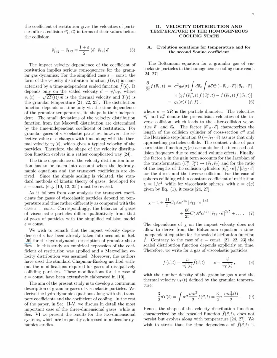
the coefficient of restitution gives the velocities of parti-cles after a collision ~v ′

1, ~v′

2 in terms of their values beforethe collision:

~v ′

1/2 = ~v1/2 ∓1 + ε

2(~e · ~v12)~e (5)

The impact velocity dependence of the coefficient ofrestitution implies serious consequences for the granu-lar gas dynamics: For the simplified case ε = const. theform of the velocity distribution function f(~v, t) is char-

acterized by a time-independent scaled function f (~c). Itdepends only on the scaled velocity ~c = ~v/vT , where

vT (t) =√

2T (t)/m is the thermal velocity and T (t) isthe granular temperature [21, 22, 23]. The distributionfunction depends on time only via the time dependenceof the granular temperature, its shape is time indepen-dent. The small deviations of the velocity distributionfunction from the Maxwell distribution are determinedby the time-independent coefficient of restitution. Forgranular gases of viscoelastic particles, however, the ef-fective value of ε changes with time along with the ther-mal velocity vT (t), which gives a typical velocity of theparticles. Therefore, the shape of the velocity distribu-tion function evolves in a rather complicated way [24].

The time dependence of the velocity distribution func-tion has to be taken into account when the hydrody-namic equations and the transport coefficients are de-rived. Since the simple scaling is violated, the stan-dard methods of kinetic theory of gases, developed forε = const. (e.g. [10, 12, 25]) must be revised.

As it follows from our analysis the transport coeffi-cients for gases of viscoelastic particles depend on tem-perature and time rather differently as compared with thecase ε = const. Correspondingly, the behavior of gasesof viscoelastic particles differs qualitatively from thatof gases of particles with the simplified collision modelε = const.

We wish to remark that the impact velocity depen-dence of ε has been already taken into account in Ref.[26] for the hydrodynamic description of granular shearflow. In this study an empirical expression of the coef-ficient of restitution was applied and a Maxwellian ve-locity distribution was assumed. Moreover, the authorshave used the standard Chapman-Enskog method with-out the modifications required for gases of dissipativelycolliding particles. These modifications for the case ofε = const. have been extensively elaborated in [10].

The aim of the present study is to develop a continuumdescription of granular gases of viscoelastic particles. Wederive the hydrodynamic equations along with the trans-port coefficients and the coefficient of cooling. In the restof the paper, in Sec. II-V, we discuss in detail the mostimportant case of the three-dimensional gases, while inSec. VI we present the results for the two-dimensionalsystems, which are frequently addressed in molecular dy-namics studies.

II. VELOCITY DISTRIBUTION AND

TEMPERATURE IN THE HOMOGENEOUS

COOLING STATE

A. Evolution equations for temperature and for

the second Sonine coefficient

The Boltzmann equation for a granular gas of vis-coelastic particles in the homogeneous cooling state reads[24, 27]

∂

∂tf (~v1, t) = σ2g2(σ)

∫

d~v2

∫

d~eΘ (−~v12 · ~e ) |~v12 · ~e |

× [χf (~v ′′

1 , t) f (~v ′′

2 , t) − f (~v1, t) f (~v2, t)]

≡ g2(σ)I (f, f) , (6)

where σ = 2R is the particle diameter. The velocities~v ′′

1 and ~v ′′

2 denote the pre-collision velocities of the in-verse collision, which leads to the after-collision veloc-ities ~v1 and ~v2. The factor |~v12 · ~e | characterizes thelength of the collision cylinder of cross-section σ2 andthe Heaviside step-function Θ (−~v12 · ~e) assures that onlyapproaching particles collide. The contact value of paircorrelation function g2(σ) accounts for the increased col-lision frequency due to excluded volume effects. Finally,the factor χ in the gain term accounts for the Jacobian ofthe transformation (~v ′′

1 , ~v′′

2 ) → (~v1, ~v2) and for the ratioof the lengths of the collision cylinders |~v ′′

12 · ~e | / |~v12 · ~e |for the direct and the inverse collision. For the case ofspheres colliding with a constant coefficient of restitutionχ = 1/ε2, while for viscoelastic spheres, with ε = ε(g)given by Eq. (1), it reads [24, 27]

χ = 1 +11

5C1Aα

2/5 |~v12 · ~e |1/5

+66

25C2

1A2α4/5 |~v12 · ~e |2/5

+ . . . . (7)

The dependence of χ on the impact velocity does notallow to derive from the Boltzmann equation a time-independent equation for the scaled distribution functionf . Contrary to the case of ε = const. [21, 22, 23] thescaled distribution function depends explicitly on time.Therefore, we write for a gas of viscoelastic particles

f (~v, t) =n

v3T (t)

f(~c, t) ~c =~v

vT (t), (8)

with the number density of the granular gas n and thethermal velocity vT (t) defined by the granular tempera-ture:

3

2nT (t) =

∫

d~vmv2

2f(~v, t) =

3

2nmv2

T (t)

2. (9)

Hence, the shape of the velocity distribution function,characterized by the rescaled function f(~c, t), does notpersist but evolves along with temperature [24, 27]. We

wish to stress that the time dependence of f(~c, t) is

3

caused by the dependence of the factor χ on the im-pact velocity. Contrary, for a gas of simplified particles(ε = const.) we obtain χ = 1/ε2 = const. and, therefore,the rescaled distribution function is time independent,f(~c, t) = f(~c ).

For slightly dissipative particles the velocity distribu-tion function is close to the Maxwell distribution. Itmay be described by a Sonine polynomial expansion[8, 22, 23, 28]:

f(~c, t) = φ(c)

(

1 +∞∑

p=1

ap(t)Sp

(

c2)

)

, (10)

where φ(c) ≡ π−3/2 exp(

−c2)

is the scaled Maxwell dis-tribution, Sp(x) are the Sonine polynomials,

S0(x) = 1

S1(x) = −x2 +3

2

S2(x) =x2

2− 5x

2+

15

8, etc.

(11)

and ak(t) are the time-dependent Sonine coefficients,which characterize the form of the velocity distribution[23, 24]. The first Sonine coefficient is trivial, a1 = 0,due to the definition of temperature [22, 23], while theother coefficients quantify deviations of the moments

⟨

ck⟩

of the velocity distribution from the moments of theMaxwell distribution

⟨

ck⟩

0, e.g.

a2 =

⟨

c4⟩

−⟨

c4⟩

0

〈c4〉0. (12)

Thus, the first nontrivial Sonine coefficient a2 character-izes the fourth moment of the distribution function.

For small enough inelasticity (ε & 0.6) the distribu-tion function is well approximated by the second Soninecoefficient a2 [22, 23, 28], i.e. higher coefficients ak = 0for k ≥ 3 may be neglected. With this approximationthe evolution a granular gas of viscoelastic particles inthe homogeneous cooling state is described by a set ofcoupled equations for the granular temperature and forthe second Sonine coefficient [24, 27]:

dT

dt= −2

3BTµ2 ≡ −ζT (13)

da2

dt=

4

3Bµ2 (1 + a2) −

4

15Bµ4 . (14)

The coefficient B ≡ B(t) = vT (t)σ2g2(σ)n is propor-tional to the mean collision frequency. The moments ofthe collision integral, µ2 and µ4 read with the approxi-mation f = φ(c)

[

1 + a2(t)S2

(

c2)]

:

µp = −1

2

∫

d~c1

∫

d~c2

∫

d~eΘ (−~c12 · ~e ) |~c12 · ~e |φ (c1)

× φ (c2)

1 + a2

[

S2

(

c21)

+ S2

(

c22)]

+ a22 S2

(

c21)

S2

(

c22)

× ∆(c p1 + c p

2 ) (15)

where

∆ψ (~ci) ≡ ψ(~c ′i ) − ψ(~ci) (16)

denotes the change of some function ψ (~ci) according toa collision. The coefficients µp depend on time via thetime dependence of a2. For small enough dissipation themoments µ2 and µ4 may be obtained as expansions inthe time-dependent dissipative parameter δ ′,

δ ′(t) ≡ Aα2/5 [2T (t)]1/10 ≡ δ

[

2T (t)

T0

]1/10

, (17)

with δ ≡ Aα2/5T1/100 and with the initial temperature

T0. These expansions read [24, 27]

µ2 =

2∑

k=0

2∑

n=0

Aknδ′ kan

2

µ4 =

2∑

k=0

2∑

n=0

Bknδ′ kan

2

(18)

where Akn and Bkn are numerical coefficients. They maybe written in the compact matrix notation (rows refer tothe first index):

A =

0 0 0

ω0625ω0

212500ω0

−ω1 − 119400ω1 − 4641

640000ω1

B =

0 4√

2π 18

√2π

285 ω0

903125ω0 − 567

12500ω0

− 7710ω1 − 476973

44000 ω1445983370400000ω1

(19)

with

ω0 ≡ 2√

2π21/10Γ

(

21

10

)

≈ 6.485

ω1 ≡√

2π21/5Γ

(

16

5

)

C21 ≈ 9.285 .

(20)

The coupled equations (13) and (14) together with (17),(18) and (19) determine the evolution of a granular gasof viscoelastic particles in the homogeneous cooling state.In particular, they define the velocity distribution func-tion which is the starting point for the investigation ofinhomogeneous gases.

B. Adiabatic approximation for the second Sonine

coefficient

In the limit of small dissipation, δ ≪ 1, the coupledequations (13),(14) may be solved analytically. In linear

4

approximation with respect to δ the solution reads [24,27]

T (t)

T0=

(

1 +t

τ0

)

−5/3

(21)

where we introduce the characteristic time

τ−10 =

16

5q0δτc(0)−1 =

48

5q0δ 4σ2n

√

πT0

m, (22)

with the initial mean collision time τc(0) and the constant

q0 = 21/5Γ

(

21

10

)

C1

8≈ 0.173 . (23)

Correspondingly in linear approximation the second So-nine coefficient depends on time as [24]

a2(t) = −12

5w(t)−1 Li [w(t)] − Li [w(0)] , (24)

with

w(t) ≡ exp

[

(q0δ)−1

(

1 +t

τ0

)1/6]

(25)

and with the logarithmic integral

Li(x) ≡∫ x

0

1

ln(t)dt . (26)

For small dissipation δ the time dependence of a2 re-veals two different regimes: (i) fast initial relaxation onthe mean collision-time scale ∼ τc(0) and (ii) subsequentslow evolution on the time scale ∼ τ0 ≫ τc(0), i.e. on thetime scale of the temperature evolution. Therefore thecoefficient a2 (and hence the form of the velocity distri-bution function) evolves in accordance with temperature.

For the hydrodynamic description of granular gases weassume that there exist well separated time and lengthscales. The short time and length scales are given bythe mean collision time and the mean free path, and thelong time and length scales are characterized by the evo-lution of the hydrodynamic fields (to be defined in thenext section) and their spatial inhomogeneities. The hy-drodynamic approach corresponds to the coarse-graineddescription of the system, where all processes which takeplace on the short time and length scales are neglected.Therefore the first stage of the relaxation of the velocitydistribution function does not affect the hydrodynamicdescription and only the second stage of its evolution onthe time scale τ0 ≫ τc(0) is to be taken into account.To this end we apply an adiabatic approximation: Weomit the term da2/dt in the left-hand side of Eq. (14)which describes the fast relaxation and assume that a2 isdetermined by the current values of µ2 and µ4 due to thepresent temperature. Hence, in the adiabatic approxima-tion a2 is determined by

5µ2 (1 + a2) − µ4 = 0 . (27)

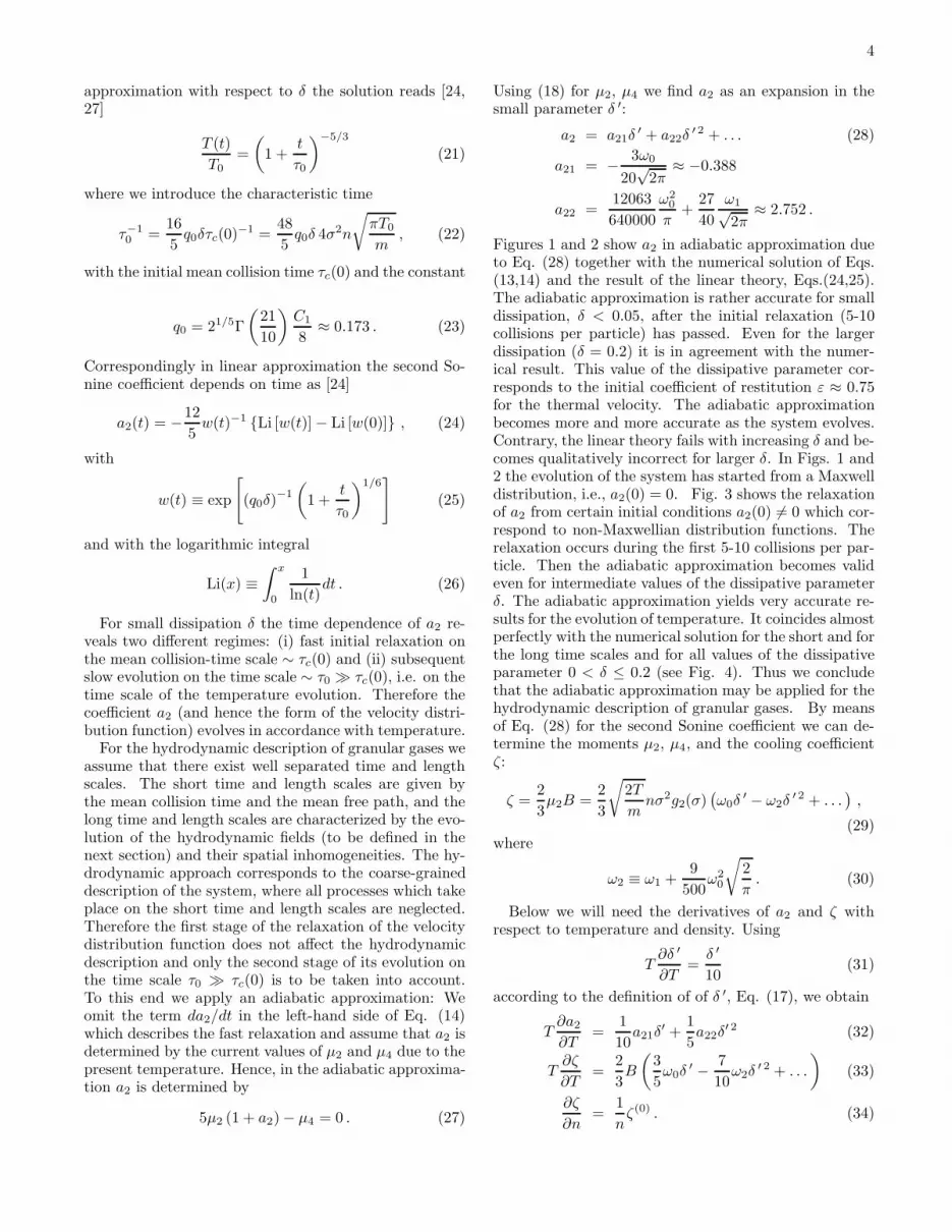
Using (18) for µ2, µ4 we find a2 as an expansion in thesmall parameter δ ′:

a2 = a21δ′ + a22δ

′ 2 + . . . (28)

a21 = − 3ω0

20√

2π≈ −0.388

a22 =12063

640000

ω20

π+

27

40

ω1√2π

≈ 2.752 .

Figures 1 and 2 show a2 in adiabatic approximation dueto Eq. (28) together with the numerical solution of Eqs.(13,14) and the result of the linear theory, Eqs.(24,25).The adiabatic approximation is rather accurate for smalldissipation, δ < 0.05, after the initial relaxation (5-10collisions per particle) has passed. Even for the largerdissipation (δ = 0.2) it is in agreement with the numer-ical result. This value of the dissipative parameter cor-responds to the initial coefficient of restitution ε ≈ 0.75for the thermal velocity. The adiabatic approximationbecomes more and more accurate as the system evolves.Contrary, the linear theory fails with increasing δ and be-comes qualitatively incorrect for larger δ. In Figs. 1 and2 the evolution of the system has started from a Maxwelldistribution, i.e., a2(0) = 0. Fig. 3 shows the relaxationof a2 from certain initial conditions a2(0) 6= 0 which cor-respond to non-Maxwellian distribution functions. Therelaxation occurs during the first 5-10 collisions per par-ticle. Then the adiabatic approximation becomes valideven for intermediate values of the dissipative parameterδ. The adiabatic approximation yields very accurate re-sults for the evolution of temperature. It coincides almostperfectly with the numerical solution for the short and forthe long time scales and for all values of the dissipativeparameter 0 < δ ≤ 0.2 (see Fig. 4). Thus we concludethat the adiabatic approximation may be applied for thehydrodynamic description of granular gases. By meansof Eq. (28) for the second Sonine coefficient we can de-termine the moments µ2, µ4, and the cooling coefficientζ:

ζ =2

3µ2B =

2

3

√

2T

mnσ2g2(σ)

(

ω0δ′ − ω2δ

′ 2 + . . .)

,

(29)where

ω2 ≡ ω1 +9

500ω2

0

√

2

π. (30)

Below we will need the derivatives of a2 and ζ withrespect to temperature and density. Using

T∂δ ′

∂T=δ ′

10(31)

according to the definition of of δ ′, Eq. (17), we obtain

T∂a2

∂T=

1

10a21δ

′ +1

5a22δ

′ 2 (32)

T∂ζ

∂T=

2

3B

(

3

5ω0δ

′ − 7

10ω2δ

′ 2 + . . .

)

(33)

∂ζ

∂n=

1

nζ(0) . (34)

5

0 5 10 15time [τ c]

-2

-1,5

-1

-0,5

0a 2 [

x100

]δ=0.01

δ=0.05

0 5 10 15time [τ c]

-3

-2

-1

0

a 2 [x1

00]

δ=0.1

0 5 10 15time [τ c]

-6

-4

-2

0

2

4

a 2 [x1

00] δ=0.2

FIG. 1: Evolution of the second Sonine coefficient a2 in thehomogeneous cooling state on the short time scale. Solid line– numerical solution of Eqs.(13,14), dashed line – adiabaticapproximation (28), dot-dashed line – the result of the lineartheory, Eqs.(24,25). The time is given in collision units τc(0).

100

101

102

103

104

105

time [τ c]

-2

-1,5

-1

-0,5

0

a 2 [x1

00]

δ=0.01

δ=0.05

100

101

102

103

104

105

time [τ c]

-3

-2

-1

0

a 2 [x1

00]

δ=0.1

100

101

102

103

104

105

time [τ c]

-6

-4

-2

0

2

4

a 2 [x1

00] δ=0.2

FIG. 2: The same as in Fig. 1, but for longer time. Theadiabatic approximation improves as the system evolves.

III. HYDRODYNAMIC EQUATIONS AND

TRANSPORT COEFFICIENTS

A. Derivation of hydrodynamic equations

For the derivation of hydrodynamic equations from theBoltzmann equation it is assumed that there exist wellseparated time and length scales. As already briefly dis-

6

0 2 4 6 8 10 12time [τ c]

-4

-2

0

2

4a 2 [

x100

]δ=0.01

0 2 4 6 8 10 12time [τ c]

-4

-2

0

2

4

a 2 [x1

00]

δ=0.2

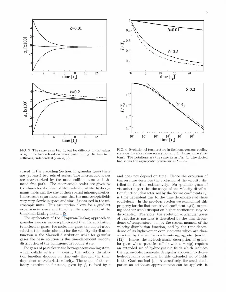
FIG. 3: The same as in Fig. 1, but for different initial valuesof a2. The fast relaxation takes place during the first 5-10collisions, independently on a2(0).

cussed in the preceding Section, in granular gases thereare (at least) two sets of scales: The microscopic scalesare characterized by the mean collision time and themean free path. The macroscopic scales are given bythe characteristic time of the evolution of the hydrody-namic fields and the size of their spatial inhomogeneities.Hence, scale separation means that the macroscopic fieldsvary very slowly in space and time if measured in the mi-croscopic units. This assumption allows for a gradientexpansion in space and time, i.e. the application of theChapman-Enskog method [5].

The application of the Chapman-Enskog approach togranular gases is more sophisticated than its applicationto molecular gases: For molecular gases the unperturbedsolution (the basic solution) for the velocity distributionfunction is the Maxwell distribution while for granulargases the basic solution is the time-dependent velocitydistribution of the homogeneous cooling state.

For gases of particles in the homogeneous cooling state,which collide with ε = const., the velocity distribu-tion function depends on time only through the time-dependent characteristic velocity. The shape of the ve-locity distribution function, given by f , is fixed by ε

0 5 10 15 20time [τ c]

0

0,2

0,4

0,6

0,8

1

T /

T0

δ=0.01

δ=0.2

100

101

102

103

104

105

time [τ c]

10-8

10-6

10-4

10-2

T /

T0

~t -5/3

δ=0.2

FIG. 4: Evolution of temperature in the homogeneous coolingstate on the short time scale (top) and for longer time (bot-tom). The notations are the same as in Fig. 1. The dottedline shows the asymptotic power-law at t → ∞.

and does not depend on time. Hence the evolution oftemperature describes the evolution of the velocity dis-tribution function exhaustively. For granular gases ofviscoelastic particles the shape of the velocity distribu-tion function, characterized by the Sonine coefficients ak,is time dependent due to the time dependence of thesecoefficients. In the previous section we exemplified thisproperty for the first non-trivial coefficient a2(t), assum-ing that for small dissipation higher coefficients may bedisregarded. Therefore, the evolution of granular gasesof viscoelastic particles is described by the time depen-dence of temperature, i.e., by the second moment of thevelocity distribution function, and by the time depen-dence of its higher-order even moments which are char-acterized by the Sonine coefficients a2, a3, etc. [see Eq.(12)]. Hence, the hydrodynamic description of granu-lar gases whose particles collide with ε = ε(g) requiresan extended set of hydrodynamic fields which includesthe higher-order moments. A regular approach to derivehydrodynamic equations for this extended set of fieldsis the Grad method [4]. Alternatively, for small dissi-pation an adiabatic approximation can be applied: It

7

is assumed that the shape of the velocity distributionfunction, albeit varying in time, follows adiabatically thecurrent temperature. Correspondingly, the higher-ordermoments are determined by the temperature too. Withthis approximation a closed set of hydrodynamic equa-tions for density n(~r, t), velocity ~u(~r, t), and temperatureT (~r, t) may be derived. These fields are defined respec-tively by the zeroth, first, and second moments of thevelocity distribution function:

n (~r, t) =

∫

d~vf (~r, ~v, t)

n (~r, t) ~u (~r, t) =

∫

d~v ~vf (~r, ~v, t) ,

3

2n (~r, t) T (~r, t) =

∫

d~v1

2mV 2f (~r, ~v, t) ,

(35)

where ~V ≡ ~v − ~u(~r, t). For small dissipation the veloc-ity distribution is well approximated by the second So-nine coefficients a2(t), i.e., higher-order coefficients areneglected. In adiabatic approximation a2 is determinedby temperature according to (28).

For simplicity of the notation we consider a dilute gran-ular gas and approximate the Enskog factor g2(σ) ≈ 1.Multiplying the Boltzmann equation for an inhomoge-neous gas

(

∂

∂t+ ~v1 · ~∇

)

f(~r, ~v1, t) = I (f, f) , (36)

correspondingly by v01 , ~v1, mv

21/2, and integrating over

d~v1 we obtain the hydrodynamic equations (see e.g. [5])

∂n

∂t+ ~∇ · (n~u ) = 0 , (37)

∂~u

∂t+ ~u · ~∇~u+ (nm)−1~∇ · P = 0 , (38)

∂T

∂t+ ~u · ~∇T +

2

3n

(

P : ~∇~u+ ~∇ · ~q)

+ ζT = 0 . (39)

The cooling coefficient ζ in the sink term ζT may bewritten as

ζ (~r, t) =σ2m

12nT

∫

d~v1

∫

d~v2

∫

d~eΘ (−~v12 · ~e ) |~v12 · ~e |

× f (~r, ~v1, t) f (~r, ~v2, t) (~v12 · ~e )2(

1 − ε2)

. (40)

The pressure tensor P and the heat flux ~q are defined by

Pij (~r, t) =

∫

Dij

(

~V)

f (~r, ~v, t) d~v + pδij (41)

~q (~r, t) =

∫

~S(

~V)

f (~r, ~v, t) d~v , (42)

where p = nT is the hydrostatic pressure. The velocity

tensor Dij and the vector ~S read

Dij(~V ) ≡ m

(

ViVj −1

3δijV

2

)

(43)

~S(

~V)

≡(

mV 2

2− 5

2T

)

~V . (44)

The structure of the hydrodynamic equations, except forthe cooling term ζT , coincides with those for moleculargases.

B. Chapman-Enskog approach

The system (37,38,39) is closed by expressing the pres-sure tensor and the heat flux in terms of the hydrody-namic fields and the fields gradients. To this end weapply the Chapman-Enskog approach [5]. This methodis based on two important assumptions: The evolutionof the distribution function is completely determined bythe evolution of its first few moments, i.e., it depends onspace and time only through the hydrodynamic fields:

f (~r, ~v, t) = f [~v, n (~r, t) , ~u (~r, t) , T (~r, t)] . (45)

As the second precondition it is assumed that the gasis only slightly inhomogeneous on the microscopic lengthscale which allows for a gradient expansion of the velocitydistribution function:

f = f (0) + λf (1) + λ2f (2) + . . . , (46)

where each power k of the formal parameter λ corre-sponds to the order k in the spatial gradient. Thus, f (0)

refers to the homogeneous cooling state, f (1) correspondsto the linear approximation with respect to the fields gra-dients, f (2) is the solution with respect to quadratic termsin the field gradients, etc. With these assumptions theBoltzmann equation may be solved iteratively for eachorder in λ, together with the hydrodynamic equations forthe moments of the velocity distribution function. Thesolution in zeroth order in λ yields the velocity distri-bution function for the homogeneous cooling state f (0)

and the corresponding evolution of temperature. Thefunction f (0) is then used to compute P and ~q, yieldingP (0) = δijp, ~q

(0) = 0 and the hydrodynamic equationsfor the ideal fluid. These first-order equations containonly linear gradient terms. Then f (1) may be found em-ploying the first-order hydrodynamic equations and thedistribution function f (0). The obtained f (1) as well asthe corresponding expressions for P (1) and ~q (1) are linearin the field gradients:

Pij =pδij − η

(

∇iuj + ∇jui −2

3δij ~∇ · ~u

)

~q = − κ~∇T − µ~∇n .(47)

The transport coefficients η, κ and µ in these equa-tions are expressed in terms of f (1). Hence, within theChapman-Enskog approach for each order in the gradi-ent expansion a closed set of equations may be derived.Keeping only first-order field gradients for the distribu-tion function and respectively for the pressure tensor andfor the heat flux as in Eq. (47), the Navier-Stokes hydro-dynamics is obtained. Keeping next-order gradient termscorresponds to the Burnett or super-Burnett description.

8

We will restrict ourselves to the Navier-Stokes level [32]and skip for simplicity of the notation the superscript“(1)” for P and ~q in the above equations.

The Chapman-Enskog scheme also assumes a hierar-chy of time scales and respectively a hierarchy of timederivatives:

∂

∂t=∂(0)

∂t+ λ

∂(1)

∂t+ λ2 ∂

(2)

∂t+ . . . , (48)

where each order k in the time derivative, ∂(k)/∂t ≡ ∂(k)t

corresponds to the related order in the space gradient.Consequently, the higher the order in the space gradient,the slower is the according time variation. Using the for-mal expansion parameter λ we can write the Boltzmannequation,

(

∂(0)

∂t+ λ

∂(1)

∂t+ . . . λ~v1 · ~∇

)

(

f (0) + λf (1) + . . .)

= I[(

f (0) + λf (1) + . . .)

,(

f (0) + λf (1) + . . .)]

(49)

and collect terms of the same order in λ. The equationin zeroth order

∂(0)

∂tf (0) = I

(

f (0), f (0))

(50)

coincides with Eq. (6) for the homogeneous cooling state.According to the Chapman-Enskog scheme we obtain thevelocity distribution function in zeroth order:

f (0) (~v,~r, t) =n (~r, t)

v3T (~r, t)

[

1 + a2S2

(

c2)]

φ(c) , (51)

where ~c = (~v − ~u) /vT = ~V /vT . The corresponding hy-drodynamic equations in this order read

∂(0)

∂tn = 0,

∂(0)

∂t~u = 0,

∂(0)

∂tT = −ζ(0)T , (52)

where ζ(0) is to be calculated using Eq. (40) with f =f (0). In this way we reproduce the previous result (29).

Collecting terms of the order O(λ) we obtain,

∂(0)f (1)

∂t+

(

∂(1)

∂t+ ~v1 · ~∇

)

f (0) + J (1)(

f (0), f (1))

= 0 ,

(53)where we introduce

−J (1)(

f (0), f (1))

≡ I(

f (0), f (1))

+I(

f (1), f (0))

. (54)

The corresponding first-order hydrodynamic equationsread

∂(1)n

∂t= − ~∇ (n~u)

∂(1)~u

∂t= − ~u · ~∇~u− 1

nm~∇p

∂(1)T

∂t= − ~u · ~∇T − 2

3T ~∇ · ~u− ζ(1)T .

(55)

The term ζ(1) is found by substituting f = f (0) + λf (1)

into Eq. (40) and collecting terms of the order O(λ).These terms contain the factor f (0) (~v,~r, t) f (1) (~v,~r, t) inthe integrand. They vanish upon integration accordingto the different symmetry of the functions f (0) and f (1),thus, ζ(1) = 0 [33].

Since the distribution function f (0) is known, we canevaluate those terms in (53) which depend only on f (0):

(

∂(1)

∂t+ ~v1 · ~∇

)

f (0) =∂f (0)

∂n

(

∂(1)n

∂t+ ~v1 · ~∇n

)

+∂f (0)

∂~u·(

∂(1)~u

∂t+ ~v1 · ~∇~u

)

+∂f (0)

∂T

(

∂(1)

∂tT + ~v1 · ~∇T

)

. (56)

With ~v1 = ~V +~u, the time derivatives of n, ~u and T givenin (55), and the relations

∂f (0)

∂n=

1

nf (0),

∂f (0)

∂~u= −∂f

(0)

∂~V, (57)

which follow from Eq. (51), we recast Eq. (53) for f (1)

into the form:

∂(0)f (1)

∂t+J (1)

(

f (0), f (1))

= f (0)(

~∇ · ~u− ~V · ~∇ logn)

+∂f (0)

∂T

(

2

3T ~∇ · ~u− ~V · ~∇T

)

+∂f (0)

∂Vi

(

(

~V · ~∇)

ui −1

nm∇i p

)

, (58)

where we take into account ζ(1) = 0.The right-hand side is known since it contains only

f (0). It is convenient, however to rewrite it in a formwhich shows explicitly the dependences on the fields gra-dients. Employing

1

nm∇ip =

T

m∇i logT +

T

m∇i logn , (59)

the right-hand side of (58) yields

∂(0)f (1)

∂t+ J (1)

(

f (0), f (1))

= ~A · ~∇ logT + ~B · ~∇ logn+ Cij∇jui , (60)

with

~A(~V ) = −~V T ∂f(0)

∂T− T

m

∂f (0)

∂~V(61)

~B(~V ) = −~V f (0) − T

m

∂

∂~Vf (0) (62)

Cij(~V ) =∂

∂Vi

(

Vjf(0))

+2T

3δij∂f (0)

∂T. (63)

9

We will calculate these terms below. From the form ofthe right-hand side of Eq. (60) we expect the form of itssolution

f (1) = ~α · ~∇ logT + ~β · ~∇ logn+ γij∇jui , (64)

which is the most general form of a scalar function, which

depends linearly on the vectorial gradients ~∇T , ~∇n and

on the tensorial gradients ∇jui. The coefficients ~α, ~β and

γij are functions of ~V and of the hydrodynamic fields n,~u and T .

We derive now equations for the coefficients ~α, ~β andγij by substituting f (1) as given by Eq. (64) into thefirst-order equation (60) and equating the coefficients of

the corresponding gradients. To this end we need ∂(0)t f (1)

and, therefore, the time derivatives of the coefficients ~α,~β, and γij :

∂(0)~α

∂t=∂~α

∂T

∂(0)T

∂t+∂~α

∂n

∂(0)n

∂t+∂~α

∂ui

∂(0)T

∂t

= −ζ(0)T∂~α

∂T, (65)

where we use Eqs. (52) in zeroth order. Similarly weobtain

∂(0)~β

∂t= −ζ(0)T

∂~β

∂T,

∂(0)γij

∂t= −ζ(0)T

∂γij

∂T(66)

and, respectively, the time-derivatives of the gradients

∂(0)

∂t~∇ logn =0

∂(0)

∂t∇jui =0

∂(0)

∂t~∇ logT = − ~∇ζ(0)

= −(

∂ζ(0)

∂n

)

~∇n−(

∂ζ(0)

∂T

)

~∇T .

(67)

The derivatives of ζ(0) are given by Eqs. (33,34). From(65), (66), and (67) we obtain:

∂(0)f (1)

∂t= −

(

T∂ζ(0)

∂T~α

)

· ~∇ log T

−(

ζ(0)T∂~β

∂T+ ζ(0)~α

)

· ~∇ logn− ζ(0)T∂γij

∂T∇jui .

(68)

where we use Eq.(34). If we insert ∂(0)t f (1) into Eq. (60)

and equate the coefficients of the gradients we arrive at

a set of equations for the coefficients ~α, ~β and γij :

− T∂ζ(0)

∂T~α+ J (1)

(

f (0), ~α)

= ~A (69)

−ζ(0)T∂~β

∂T− ζ(0)~α+ J (1)

(

f (0), ~β)

= ~B (70)

−ζ(0)T∂γij

∂T+ J (1)

(

f (0), γij

)

= Cij (71)

where J (1) is defined by Eq. (54).

C. Kinetic coefficients in terms of the velocity

distribution function

From the definition of the pressure tensor Eq. (41)and its expression in terms of the field gradients Eq. (47)follows

∫

Dij

(

f (0) + ~α · ~∇ logT + ~β · ~∇ logn+ γkl∇luk

)

d~V

= −η(

∇iuj + ∇jui −2

3δij ~∇ · ~u

)

, (72)

where the tensor Dij

(

~V)

has been defined above. The

integrals

∫

Dijf(0)d~V =

∫

Dij~α d~V =

∫

Dij~β d~V = 0 (73)

vanish since Dij is a traceless tensor and f (0) depends

isotropically on ~V . Moreover, as will be shown below,

the vectors ~α and ~β are directed along ~V , hence, the

respective integrands are odd functions of ~V . Therefore,only the term with the factor γkl∇luk in the left-handside of Eq. (72) is non-trivial. Equating the coefficientsof the gradient factor ∇luk we obtain

∫

Dijγkld~V = −η(

δliδkj + δljδki −2

3δijδkl

)

. (74)

For k = j, l = i the last equation turns into

∫

Dijγjid~V = −η(

δiiδjj + δijδij −2

3δijδij

)

= −10η ,

(75)(δiiδjj = 9 and δijδij = 3 according to the summationconvention) and yields the coefficients of viscosity

η = − 1

10

∫

Dij

(

~V)

γji

(

~V)

d~V . (76)

Using Eq. (41) for the heat flux and its corresponding ex-pression in terms of the field gradients, Eq. (47), we canperform a completely analogous calculation and arrive atthe kinetic coefficients κ and µ:

κ = − 1

3T

∫

d~V ~S(

~V)

· ~α(

~V)

(77)

µ = − 1

3n

∫

d~V ~S(

~V)

· ~β(

~V)

, (78)

with ~S defined by Eq. (44). The coefficient of thermalconductivity κ has the standard interpretation, while theother coefficient µ does not have an analog for moleculargases.

10

IV. COEFFICIENT OF VISCOSITY

The viscosity coefficient is related to the coefficient γij

[see Eq. (76)] which, in its turn, is the solution of Eq.(71) with the coefficient Cij in the right-hand side. Letus first find an explicit expression for Cij .

According to Eq. (51) the velocity distribution func-tion depends on temperature through the thermal veloc-ity vT and additionally through the second Sonine coeffi-cient a2. Hence the temperature derivative of f (0) reads

∂f (0)

∂T=

1

2T

∂

∂~V· ~V f (0) + fM (V )S2

(

c2) ∂a2

∂T, (79)

with fM (V ) being the Maxwell distribution

fM =n

v3T

φ(c) with φ(c) =1

π3/2exp

(

−c2)

. (80)

Using the relation

∂f (0)

∂Vi=Vi

V

∂f (0)

∂V(81)

and Eq. (79) the coefficient Cij reads

Cij

(

~V)

=

(

ViVj −1

3δijV

2

)

1

V

∂f (0)

∂V

+2

3δijS2

(

c2)

fM (V )T∂a2

∂T. (82)

With

1

V

∂f (0)

∂V= −m

T

[

1 + a2S2

(

c2)]

fM +m

T

(

c2 − 5

2

)

a2 fM

(83)we obtain

Cij = − 1

TDij

[

1 + a2

(

S2

(

c2)

+5

2− c2

)]

fM (V )

+2

3δijS2

(

c2)

fM (V )T∂a2

∂T, (84)

where Dij

(

~V)

has been defined in Eq. (43).

The expression for Cij determines the right-hand sideof Eq. (71) for γij and hence it suggests the form forγij . For small dissipation (when a2 is small) and forsmall fields gradients we keep only the leading terms withrespect to these variables. Therefore, we seek for γij inthe form

γij

(

~V)

=γ0

TDij

(

~V)

fM (V ) , (85)

where γ0 is a velocity-independent coefficient, i.e., weneglect the dependence of γij on a2 [34]. The viscositycoefficient Eq. (76) reads then

η = −γ0

10

1

T

∫

d~V DijDijfM = −γ0nT , (86)

where we take into account that

DijDji =2

3m2V 4 (87)

according the definition of Dij , Eq. (43), with the sum-mation convention. Moreover, we have used the fourthmoment of the Maxwell distribution. From Eq. (86) fol-lows

γ0 = − η

nT. (88)

Multiplying Eq. (71) by Dij(~V1), integrating over ~V1

and using Eq. (76) yields

− 10ζ(0)T∂η

∂T= −

∫

d~V1Dij

(

~V1

)

Cij

(

~V1

)

+

∫

d~V1Dij

(

~V1

)

J (1)(

f (0), γij

)

. (89)

To evaluate the first term in the right-hand side we useEq. (63) for Cij , the relation

∂

∂ViDij =

∂

∂Vim

(

ViVj −1

3δijV

2

)

= mVj

(

1 +1

3δij

)

,

(90)the definition of temperature, Eq. (35), and notice thatDijδij = 0 since Dij is a traceless tensor [see Eq. (43)].Integration by parts then yields

∫

d~V1Dij Cij = (91)

=

∫

d~V1Dij∂

∂V1iV1jf

(0) +2T

3

∫

d~V1Dijδij∂f (0)

∂T

=

∫

d~V1f(0)mV1jV1j

(

1 +1

3δij

)

=10

3

∫

d~V1f(0)mV 2

1

= 10nT .

For the second term in the right-hand side of (89) we usethe definition of J (1), (54), and obtain

∫

d~V1DijJ(1)(

f (0), γij

)

= −∫

d~V1DijI(

f (0), γij

)

−∫

d~V1DijI(

γij , f(0))

.

(92)

We apply the property of the collision integral [5]

∫

d~V1DijI(

f (0), γij

)

=

∫

d~V1DijI(

γij , f(0))

=σ2

2

∫

d~V1

∫

d~V2f(0)(

~V1

)

γij

(

~V2

)

∫

d~eΘ(

−~V12 · ~e)

×∣

∣

∣

~V12 · ~e∣

∣

∣∆[

Dij

(

~V1

)

+Dij

(

~V2

)]

, (93)

11

where ∆ψ (~vi) ≡ ψ (~v ′

i )−ψ (~vi) denotes as previously thechange of some quantity ψ(~vi) due to a collision. Equa-tion (92) turns then into

∫

d~V1DijJ(1)(

f (0), γij

)

= −σ2

∫

d~V1

∫

d~V2f(0)(

~V1

)

× γij

(

~V2

)

∫

d~eΘ(

−~V12 · ~e) ∣

∣

∣

~V12 · ~e∣

∣

∣

∆[

Dij

(

~V1

)

+Dij

(

~V2

)]

. (94)

We write the factors in the last integral using the dimen-

sionless velocities ~V1/2 = vT~c1/2:

Dij

(

~V)

=mv2TDij (~c ) = mv2

T

(

cicj −1

3δijc

2

)

γij

(

~V)

=γ0

T

(

n

v3T

)

mv2TDij (~c )φ (c) ,

(95)

and recast Eq. (94) into the form

∫

d~V1Dij

(

~V1

)

J (1)(

f (0), γij

)

= 4ηvTnσ2Ωη , (96)

where we substitute γ0 = −η/nT and where Ωη is a nu-merical coefficient defined by

Ωη ≡∫

d~c1

∫

d~c2

∫

d~eΘ (−~c12 · ~e ) |~c12 · ~e | f (0) (c1)

× φ (c2)Dij (~c2)∆ [Dij (~c1) +Dij (~c2)] . (97)

The coefficient Ωη may be expressed in terms of the dis-sipation parameter δ′ and the second Sonine coefficienta2 (see Appendix):

Ωη = −(

w0 + δ′w1 − δ′ 2w2

)

(98)

with

w0 =4√

2π

(

1 − 1

32a2

)

w1 =ω0

(

1

15− 1

500a2

)

w2 =ω1

(

97

165− 679

44000a2

)

.

(99)

Substituting Eqs. (91,96,98) into Eq. (89) and using Eq.(29) for ζ(0) we obtain an equation for the coefficient ofviscosity η:

(

ω0δ′ − ω2δ

′ 2)

T∂η

∂T

=3

5

(

w0 + w1δ′ − w2δ

′ 2)

η − 3

2

1

σ2

√

mT

2. (100)

We seek the solution as an expansion in terms of δ′:

η = η0(

1 + δ′η1 + δ′ 2η2 + . . .)

. (101)

The solution in zeroth order

η0 =5

16σ2

√

mT

π(102)

is the viscosity coefficient for a gas of elastic particles(Enskog viscosity), while the coefficients η1 and η2 ac-count for the dissipative properties of viscoelastic parti-cles. With Eq. (31) the temperature derivative of theviscosity coefficient reads

T∂η

∂T= η0

(

1

2+

3

5δ′η1 +

7

10δ′ 2η2 + . . .

)

. (103)

We substitute Eqs. (101,103) into Eq. (100), express a2

in terms of δ′ according to Eq. (28) and collect terms ofthe same order in δ′. This yields the equations for η1, η2,etc., whose solutions read

η1 =359

3840

√2π

πω0 ≈ 0.483

η2 =41881

2304000

ω20

π− 567

28160

ω1

√2π

π≈ 0.094 ,

(104)

with ω0/1 given by Eq. (20).Thus, we arrive at the final expression for the viscosity

coefficient for a granular gas of viscoelastic particles:

η =5

16σ2

√

mT

π

(

1 + 0.483 δ′ + 0.094 δ′2 + . . .)

. (105)

In contrast to granular gases of simplified particles (ε =

const.), where η ∝√T , for a gas of viscoelastic particles

there is an additional temperature dependence due to thetime-dependent coefficient δ′.

V. COEFFICIENT OF THERMAL

CONDUCTIVITY AND THE COEFFICIENT µ

To find coefficients κ and µ we need the coefficients

~α and ~β which are the solutions of Eqs. (69,70). The

functions ~A and ~B in the right-hand sides may be foundfrom Eqs. (61,62):

~A = − 1

T~S(

~V)

[

1 + a2

(

S2

(

c2)

+ 1 − c2)]

fM

− ~V S2

(

c2)

[a21

10δ′ +

a22

5δ′ 2]

fM (106)

~B =a2

T~S(

~V)

fM . (107)

Keeping only leading terms with respect to the gradientsand a2, we choose ~α in the form

~α = −α1

T~S(

~V)

fM (V ) , (108)

12

with α1 being the velocity independent coefficient. ThisAnsatz for ~α yields the coefficient of thermal conductiv-ity,

κ = − 1

3T

∫

d~V ~S(

~V)

· ~α(

~V)

=α1

3T 2

∫

d~V

(

mV 2

2− 5

2T

)2

V 2fM

=5

2

nT

mα1 , (109)

which implies

α1 =2m

5nTκ . (110)

Multiplying Eq. (69) for ~α by ~S(

~V1

)/

T , integrating

over ~V1 and using Eq. (77) for κ we obtain

3∂

∂Tζ(0)κT =

1

T

∫

d~V1~S · ~A− 1

T

∫

d~V1~S · J (1)

(

f (0), ~α)

.

(111)To evaluate the first term in the right-hand side we use

Eq. (44) for ~S(

~V)

and Eq. (106) for ~A(

~V)

:

− 1

T

∫

d~V ~S(

~V)

· ~A(

~V)

=

= v2T

∫

d~V

(

c2 − 5

2

)2

c2[

1 + a2

(

S2

(

c2)

+ 1 − c2)]

fM

+ v2T

∫

d~V

(

c2 − 5

2

)

c2[a21

10δ′ +

a22

5δ′ 2]

S2

(

c2)

fM .

(112)

With the Maxwell distribution Eq. (80) the first term inthe last equation (112) reads

4πnv2T

∫

∞

0

c4φ(c)

(

c2 − 5

2

)2

dc

+a2

∫

∞

0

c4φ(c)

(

c2 − 5

2

)2 [c4

2− 7c2

2+

23

8

]

dc

=15

4nv2

T +15

2nv2

T a2 =15

2

nT

m(1 + 2a2) , (113)

where integration over the angles has been performed andthe integral

∫

∞

0

exp(

−x2)

x2kdx =(2k − 1)!!

2k+1

√π (114)

was used. Very similar calculations give the second termin Eq. (112):

15

4nv2

T

(a21

10δ′ +

a22

5δ′ 2)

. (115)

Summing up Eqs. (113) and (115) we obtain the firstterm in the right-hand side of (111):

1

T

∫

d~V1~S · ~A = −15

2

nT

m

(

1 +21

10a21δ

′ +11

5a22δ

′ 2

)

.

(116)The second term in the right-hand side of Eq. (111) maybe again written using the basic property of the collisionintegral [see Eq. (93)]:

− 1

T

∫

d~V1~S(

~V1

)

· J (1)(

f (0), ~α)

=

=σ2

T

∫

d~V1

∫

d~V2f(0)(

~V1

)

~α(

~V2

)

·∫

d~eΘ(

−~V12 · ~e)

×∣

∣

∣

~V12 · ~e∣

∣

∣∆[

~S(

~V1

)

+ ~S(

~V2

)]

. (117)

Using the dimensionless variables

~S(

~V)

= vTT ~S (~c) = vTT

(

c2 − 5

2

)

~c

~α(

~V)

= −α1 vT

(

n

~v 3T

)

φ(c)~S (~c )

(118)

and Eq. (110) for α1, we recast the last equation into theform

− 1

T

∫

d~V ~S(

~V)

·J (1)(

f (0), ~α)

= −4

5κvTnσ

2Ωκ . (119)

The coefficient Ωκ is defined by

Ωκ ≡∫

d~c1

∫

d~c2

∫

d~eΘ (−~c12 · ~e ) |~c12 · ~e| f (0) (c1)

× φ (c2) ~S (~c2) · ∆[

~S (~c1) + ~S (~c2)]

. (120)

This coefficient reads (see Appendix)

Ωκ = −(

u0 + δ′u1 − δ′ 2u2

)

(121)

where

u0 =4√

2π

(

1 +1

32a2

)

u1 =ω0

(

17

5− 9

500a2

)

u2 =ω1

(

1817

440− 1113

352000a2

)

.

(122)

Substituting Eqs. (116,119,121) into Eq. (111) and usingEq. (29) for ζ(0) we arrive at

T∂

∂TκT 3/2

(

ω0δ′ − ω2δ

′ 2 + . . .)

=2

5κT 3/2

(

u0 + δ′u1 − δ′ 2u2 + . . .)

− 15

4

T 3/2

σ2

√

T

2m

(

1 +21

10a21δ

′ +11

5a22δ

′ 2

)

. (123)

13

We solve this equation with the Ansatz

κ = κ0

(

1 + δ′κ1 + δ′ 2κ2 + . . .)

, (124)

where

κ0 =75

64σ2

√

T

πm(125)

is the Enskog thermal conductivity for a gas of elasticparticles. Substituting Eq. (124) into Eq. (123) andequating terms of the same order in δ′ we obtain thecoefficients

κ1 =487

6400

√2πω0

π≈ 0.393

κ2 =1

π

(

2872113

51200000ω2

0 +78939

140800

√2πω1

)

≈ 4.904 .

(126)

Hence, the coefficient of thermal conductivity for a gran-ular gas of viscoelastic particles reads in adiabatic ap-proximation

κ =75

64σ2

√

T

πm

(

1 + 0.393δ′ + 4.904δ′2 + . . .)

. (127)

Similar to the viscosity coefficient, the coefficient of ther-mal conductivity of a granular gas of viscoelastic particlesreveals an additional temperature dependence as com-pared with gases of simplified particles where ε = const.

The evaluation of the coefficient µ may be performed

in the same way as κ, i.e. choosing ~β in the form

~β = −β1

T~S(

~V)

fM (V ) , (128)

with the velocity independent coefficient ~β. The onlydifference is that the expansion of µ in terms of the dissi-pative parameter δ′ lacks the term in zeroth order sinceµ vanishes in the elastic limit. Since the calculations arecompletely analogous to that for κ, we present here onlythe final result:

µ =κ0T

n

(

δ′µ1 + δ′ 2µ2 + . . .)

(129)

with

µ1 =19

80

ω0

√2π

π≈ 1.229

µ2 =1

π

(

58813

640000ω2

0 − 1

40

√2πω1

)

≈ 1.415 .

(130)

Thus, the coefficient µ reads in adiabatic approximation

µ =κ0T

n

(

1.229 δ′ + 1.415 δ′2 + . . .)

(131)

Finally, using the coefficients

α1 =2m

5nTκ , β1 =

2m

5T 2µ , γ0 = − 1

nTη , (132)

(the result for β1 may be derived analogously as for α1)

in the relations (108,128,85) for ~α, ~β, γij we obtain an

expression for the first-order distribution function f (1),which depends linearly on the field gradients accordingto Eq. (64).

VI. TWO-DIMENSIONAL GRANULAR GAS

So far we have restricted ourselves to three-dimensionalsystems although the calculations are identical for gen-eral dimension d. Of particular interest is the case d = 2.Since molecular dynamics simulations are frequently per-formed for two-dimensional systems, in this section wepresent the results for two-dimensional gases of viscoelas-tic particles. We wish to stress that these systems are, infact, quasi two-dimensional, since we still use the coeffi-cient of restitution Eq. (1) for colliding spheres. Hence,we assume that the motion of the spherical particles ofthe gas is restricted to a two-dimensional surface.

The hydrodynamic equations for two-dimensionalgases have the form

∂n

∂t+ ~∇ · (n~u) = 0

∂~u

∂t+ ~u · ~∇~u+ (nm)−1 ~∇ · P = 0

∂T

∂t+ ~u · ~∇T +

1

n

(

Pij∇jui + ~∇ · ~q)

+ ζ T = 0 ,

(133)

with the pressure tensor and the heat flux

Pij = nTδij − η(

∇iuj + ∇jui − δij ~∇ · ~u)

~q = −κ~∇T − µ~∇n .(134)

Correspondingly, the transport coefficients read

η = η0(

1 + δ′η1 + δ′ 2η2 + · · ·)

, (135)

where δ ′ (t) = δ [2T (t) /T0]1/10

and

η0 =1

2σ

√

mT

π

η1 =29

640

√2π

πω0 ≈ 0.234 (136)

η2 =111

160000

ω20

π+

569

14080

ω1

√2π

π≈ 0.308 .

Similarly,

κ = κ0

(

1 + δ′κ1 + δ′ 2κ2 + · · ·)

(137)

with

κ0 =2

σ

√

T

πm

κ1 = − 433

3200

√2πω0

π≈ −0.700 (138)

κ2 =1

π

(

1749573

12800000ω2

0 +95619

70400

√2πω1

)

≈ 11.89 .

14

and

µ =κ0T

n

(

δ′µ1 + δ′ 2µ2 + · · ·)

µ1 =7

20

ω0

√2π

π≈ 1.811 (139)

µ2 =1

π

(

− 7411

80000ω2

0 +7

40

√2πω1

)

≈ 0.056 .

The cooling rate ζ(0) reads for a two-dimensional gas ofviscoelastic particles

ζ(0) =

√

2T

mnσ

(

1

2ω0δ

′ − ω2δ′ 2 + · · ·

)

ω2 =1

2ω1 +

9√

2π

500πω2

0 ≈ 5.246 . (140)

The numerical constants ω0/1 are given by Eq. (20).

VII. SUMMARY

We have derived the hydrodynamics of granular gasesof viscoelastic particles. Collisions of viscoelastic parti-cles are characterized by an impact velocity dependentcoefficient of restitution. We have used the Chapman-Enskog approach together with an adiabatic approxima-tion for the velocity distribution function, which assumesthat the shape of the velocity distribution function fol-lows adiabatically the decaying temperature. We havecompared the numerical solutions for temperature T (t)and for the second Sonine coefficient a2(t) with the corre-sponding adiabatic approximations and have found goodagreement up to intermediate dissipation. To derive thehydrodynamic equations and transport coefficients fromthe Boltzmann equation we have modified the standardscheme to account for the time dependence of the basicsolution. This modification takes into account the timedependence not only due to the thermal velocity, as forε = const., but also due to the evolution of the shape ofthe distribution function as given for gases of viscoelasticparticles.

Transport coefficients and the cooling coefficient fordilute granular gases of viscoelastic particles read

η = η0(

1 + δ′η1 + δ′ 2η2 + . . .)

(141)

κ = κ0

(

1 + δ′κ1 + δ′ 2κ2 + . . .)

(142)

µ =κ0T

n

(

δ′µ1 + δ′ 2µ2 + . . .)

(143)

ζ(0) =nT

η0

(

δ′ζ1 + δ′ 2ζ2 + . . .)

(144)

where η0 and κ0 are the Enskog values for the viscosityand the coefficient of thermal conductivity and δ′ is thetime dependent dissipative parameter. The numericalcoefficients η1/2, κ1/2, µ1/2, and ζ1/2 are given in TableI.

TABLE I: Numerical coefficients for Eqs. (141-144)

3d 2d 3d 2d

η1 0.483 0.234 η2 0.094 0.309)

κ1 0.393 -0.700 κ2 4.904 11.893

µ1 1.229 1.811 µ2 1.415 0.056

ζ1 1.078 1.294 ζ2 -1.644 -2.093

The dependence on temperature and, therefore, ontime of the kinetic coefficients Eqs. (141)-(144) differssignificantly from the time dependence of the correspond-ing coefficients for granular gases of particles which col-lide with a simplified collisional model ε = const. Thisleads to the serious consequences for the global behaviorof force-free granular gases [29].

Under mild preconditions the presented formalism forthe derivation of the hydrodynamic equations and thetransport coefficients may be applied also to gases of par-ticles whose collision is described by a different impactvelocity dependence than given for viscoelastic particles.

APPENDIX A: DERIVATION OF THE

COEFFICIENTS Ωη AND Ωκ

For the evaluation of the numerical coefficient Eq.(97), defined by

Ωη ≡∫

d~c1

∫

d~c2

∫

d~eΘ (−~c12 · ~e ) |~c12 · ~e | f (0) (c1)

× φ (c2)Dij (~c2)∆ [Dij (~c1) +Dij (~c2)] . (A1)

we need the factor

Dij (~c2)∆ [Dij (~c1) +Dij (~c2)]

= (~c ′1 · ~c2)2+ (~c ′2 · ~c2)

2 − (~c1 · ~c2)2 − (~c2 · ~c2)2

− 1

3c22(

c′ 21 + c′ 22 − c21 − c22)

(A2)

Similarly, for the coefficient

Ωκ ≡∫

d~c1

∫

d~c2

∫

d~eΘ (−~c12 · ~e ) |~c12 · ~e | f (0) (c1)

× φ (c2) ~S (~c2) · ∆[

~S (~c1) + ~S (~c2)]

, (A3)

given by Eq. (120) we need

~S (~c2) · ∆[

~S (~c1) + ~S (~c2)]

=

(

c22 −5

2

)

[

(~c ′1 · ~c2) (c ′1)2

+ (~c ′2 · ~c2) (c ′2)2 − (~c1 · ~c2) c21 − (~c2 · ~c2) c22

]

. (A4)

15

With (A2) and (A4) we write for the coefficient Ωη

Ωη =

∫

d~c1

∫

d~c2

∫

d~eΘ (−~c12 · ~e ) |~c12 · ~e | f (0)(c1)

× φ (c2)[

(~c ′1 · ~c2)2

+ (~c ′2 · ~c2)2 − (~c1 · ~c2)2

− (~c2 · ~c2)2 −1

3c22(

c′ 21 + c′ 22 − c21 − c22)

]

. (A5)

and for the coefficient Ωκ,

Ωκ =

∫

d~c1

∫

d~c2

∫

d~eΘ (−~c12 · ~e ) |~c12 · ~e | f (0) (c1)

× φ2 (c2)

(

c22 −5

2

)

[

(~c ′1 · ~c2) (c′1)2+ (~c ′2 · ~c2) (c′2)

2

− (~c1 · ~c2) c21 − (~c2 · ~c2) c22]

. (A6)

The pre-collision velocities ~c1, ~c2 as well as after-collisionvelocities ~c ′1, ~c

′

2 can be expressed in terms of the center of

mass velocity ~C = (~c1 + ~c2) /2 and the relative velocity~c12 = ~c1 − ~c2 before the collision:

~c1 = ~C +1

2~c12

~c2 = ~C − 1

2~c12

~c ′1 = ~C +1

2~c12 −

1

2(1 + ε) (~c12 · ~e )~e

~c ′2 = ~C − 1

2~c12 +

1

2(1 + ε) (~c12 · ~e )~e .

(A7)

The coefficient of restitution is expressed in terms of therelative velocity ~c12 by

ε = 1 − C1δ′ (t) |~c12 · ~e |1/5

+3

5C2

1 δ′ 2 (t) |~c12 · ~e |2/5

+ . . .

(A8)The second Sonine polynomial in the distribution func-tion

f (0)(c1) = φ(c1)[

1 + a2S2

(

c21)]

, (A9)

reads in terms of ~C and ~c12

S2

(

c21)

=C4

2+

1

2

(

~C · ~c12)2

+1

32c412 + C2

(

~C · ~c12)

+1

4C2c212 +

1

4c212

(

~C · ~c12)

− 5

2C2

− 5

2

(

~C · ~c12)

− 5

8c212 +

15

8. (A10)

If we replace all factors in the integrands of Eqs. (A5,A6)

by the corresponding expressions in terms of ~C and ~c12we observe that Ωη and Ωκ may be written as a sum ofintegrals of the structure

Jk,l,m,n,p,α =

∫

d~c12

∫

d~C

∫

d~eΘ (−~c12 · ~e ) |~c12 · ~e |1+α

φ (c12)φ(C)Ckcl12

(

~C · ~c12)m (

~C · ~e)n

(~c12 · ~e )p.

(A11)

The solution of this integral in general dimension d reads[24] for n = 0

Jk,l,m,0,p,α = (−1)p [1 + (−1)m] 2l+m+p+α+1Ω−1d

× βp+α+1βmγk+mγl+m+p+α+1 , (A12)

for n = 1

Jk,l,m,1,p,α = (−1)p+1[

1 + (−1)m+1]

2l+m+p+α+1Ω−1d

× βp+α+2βm+1 γk+m+1γl+m+p+α+1 , (A13)

and for n = 2,

Jk,l,m,2,p,α = (−1)p [1 + (−1)m] 2l+m+p+α+1

× [(d− 1)Ωd]−1γk+m+2 γl+m+p+α+1

×[(dβp+α+3 − βp+α+1) βm+2 + (βp+α+1 − βp+α+3)βm] ,(A14)

where

Ωd =2πd/2

Γ(

d2

) (A15)

is the surface of a d-dimensional unit sphere. The coeffi-cients βm, γm read

βm = π(d−1)/2 Γ(

m+12

)

Γ(

m+d2

)

γm = 2−m/2 Γ(

m+d2

)

Γ(

d2

) .

(A16)

Following this procedure we obtain the desired coeffi-cients as given by Eqs. (98) and (121).

The evaluation of the sums which lead to the factors Ωη

and Ωκ is straightforward, however, very lengthy. Theycan be calculated by symbolic algebra [30].

[1] D. Kolymbas, ed., Constitutive modelling of granular ma-

terials (Springer, Berlin, 2000).[2] P. A. Vermeer, S. Diebels, W. Ehlers, H. Herrmann,

S. Luding, and E. Ramm, eds., Continuous and dis-

continuous modelling of cohesive-frictional materials

(Springer, Berlin, 2000).[3] T. Poschel and S. Luding, eds., Granular Gases, vol. 564

of Lecture Notes in Physics (Springer, Berlin, 2001).

16

[4] H. Grad, Comm. Pure and Appl. Math. 2, 331 (1949).[5] S. Chapman and T. G. Cowling, The Mathematical The-

ory of Non-uniform Gases (Cambridge University Press,Cambridge, 1970).

[6] C. K. K. Lun, S. B. Savage, D. J. Jeffrey, and N. Chep-urniy, J. Fluid Mech. 140, 223 (1984).

[7] J. T. Jenkins and M. W. Richman, Archives for ParticleMechanics and Analysis 87, 355 (1985).

[8] A. Goldshtein and M. Shapiro, J. Fluid Mech. 282, 75(1995).

[9] N. Sela and I. Goldhirsch, J. Fluid Mech. 361, 41 (1998).[10] J. J. Brey, J. W. Dufty, C. S. Kim, and A. Santos, Phys.

Rev. E 58, 4638 (1998).[11] J. J. Brey, M. J. Ruiz-Montero, and D. Cubero, Phys.

Rev. E 60, 3150 (1999).[12] V. Garzo and J. W. Dufty, PRE 59, 5895 (1999).[13] J. J. Brey and D. Cubero, in [3], p. 59.[14] W. Goldsmit, Impact: The theory and physical behavior

of colliding solids (Arnold, London, 1960).[15] F. G. Bridges, A. Hatzes, and D. N. C. Lin, Nature 309,

333 (1984).[16] G. Kuwabara and K. Kono, Jpn. J. Appl. Phys. 26, 1230

(1987).[17] R. Ramırez, T. Poschel, N. V. Brilliantov, and T. Schwa-

ger, Phys. Rev. E 60, 4465 (1999).[18] H. Hertz, J. f. reine u. angewandte Math. 92, 156 (1882).[19] N. V. Brilliantov, F. Spahn, J.-M. Hertzsch, and

T. Poschel, Phys. Rev. E 53, 5382 (1996).

[20] T. Schwager and T. Poschel, Phys. Rev. E 57, 650 (1998).[21] S. E. Esipov and T. Poschel, J. Stat. Phys. 86, 1385

(1997).[22] T. P. C. van Noije and M. H. Ernst, Granular Matter 1,

57 (1998).[23] N. V. Brilliantov and T. Poschel, Phys. Rev. E 61, 2809

(2000).[24] N. V. Brilliantov and T. Poschel, Phys. Rev. E 61, 5573

(2000).[25] R. Ramırez, D. Risso, R. Soto, and C. P., Phys. Rev. E

62, 2521 (2000).[26] C. K. K. Lun and S. B. Savage, Acta Mechanica 63, 15

(1986).[27] N. Brilliantov and T. Poschel, in [3], p. 100.[28] M. Huthmann, J. Orza, and R. Brito, Granular Matter

2, 189 (2000).[29] N. V. Brilliantov and T. Poschel, Phil. Trans. R. Soc.

Lond. A 360, 415 (2001).[30] T. Poschel and N. V. Brilliantov, preprint (2003).[31] I. Goldhirsch, in [3], p. 79.[32] It has been shown that some processes in granular gases

require the Burnett level to derive a consistent set ofequations [9, 31].

[33] This may be directly checked using Eq. (64) for f (1)

[34] In a more general approach γij is represented as an ex-pansion in orthogonal polynomials, with (85) being thefirst order term [5].