Accepted by the Astrophysical JournalPreprint typeset using LATEX style emulateapj v. 11/10/09

HUBBLE RESIDUALS OF NEARBY TYPE IA SUPERNOVAE ARE CORRELATED WITH HOST GALAXYMASSES

Patrick L. Kelly1,2, Malcolm Hicken3, David L. Burke1,2, Kaisey S. Mandel3, and Robert P. Kirshner3

Accepted by the Astrophysical Journal

ABSTRACT

From Sloan Digital Sky Survey u’g’ r’ i’ z’ imaging, we estimate the stellar masses of the host galaxiesof 70 low redshift SN Ia (0.015 < z < 0.08) from the hosts’ absolute luminosities and mass-to-lightratios. These nearby SN were discovered largely by searches targeting luminous galaxies, and wefind that their host galaxies are substantially more massive than the hosts of SN discovered by theflux-limited Supernova Legacy Survey. Testing four separate light curve fitters, we detect ∼2.5σcorrelations of Hubble residuals with both host galaxy size and stellar mass, such that SN Ia occurringin physically larger, more massive hosts are ∼10% brighter after light curve correction. The Hubbleresidual is the deviation of the inferred distance modulus to the SN, calculated from its apparentluminosity and light curve properties, away from the expected value at the SN redshift. Marginalizingover linear trends in Hubble residuals with light curve parameters shows that the correlations cannotbe attributed to a light curve-dependent calibration error. Combining 180 higher-redshift ESSENCE,SNLS, and HigherZ SN with 30 nearby SN whose host masses are less than 1010.8 M� in a cosmologyfit yields 1 + w = 0.22+0.152

−0.108, while a combination where the 30 nearby SN instead have host masses

greater than 1010.8 M� yields 1 + w = −0.03+0.217−0.143. Progenitor metallicity, stellar population age, and

dust extinction correlate with galaxy mass and may be responsible for these systematic effects. Hostgalaxy measurements will yield improved distances to SN Ia.Subject headings: supernovae: general

1. INTRODUCTION

SN Ia are useful probes of the cosmic expansion history(Astier et al. 2006; Wood-Vasey et al. 2007; Riess et al.2007; Hicken et al. 2009b; Kessler et al. 2009a). Theirextremely bright explosions can be detected to high red-shifts and, after calibration by light curve shape, yieldluminosity distances over a wide range of cosmic epochsspanning the past 8 Gyr. While the peak luminositiesof SN Ia vary by a factor of ∼3, more slowly-evolvingSN Ia are intrinsically brighter (Phillips 1993) and bluer(Riess et al. 1996), a pattern used to calibrate SN Ia andmeasure luminosity distances to a precision of ∼10%. Al-though initial efforts were limited by small detector sizes(Norgaard-Nielsen et al. 1989), search programs usingnewer, large format cameras discovered that distant SNIa were ∼25% fainter than expected for any matter-onlyuniverse, favoring an accelerating expansion (Riess et al.1998; Perlmutter et al. 1999). In this paper, we look forcorrelations between the Hubble residuals of nearby SNIa and their host galaxy sizes and masses.

Theoretical models of a carbon-oxygen white dwarfwith a mass approaching the Chandrasekhar limit showthat it can explode to produce a realistic SN Ia spec-trum (Hillebrandt & Niemeyer 2000; Kasen & Plewa2005; Kasen & Woosley 2007; Kasen et al. 2009). A su-personic deflagration wave, possibly preceded by a moreslowly moving carbon fusion flame, synthesizes radioac-

pkelly3@stanford.edu1 Kavli Institute for Particle Astrophysics and Cosmology,

Stanford University, 382 Via Pueblo Mall, Stanford, CA 943052 SLAC National Accelerator Laboratory, 2575 Sand Hill Rd,

Menlo Park, CA 940253 Harvard-Smithsonian Center for Astrophysics, 60 Garden

St., Cambridge, MA 02138

tive 56Ni during the explosion, and subsequent decaysto 56Co and 56Fe (Truran et al. 1967; Colgate & McKee1969) then power the SN light curve. How the progenitoraccumulates a mass close to the Chandrasekhar limit be-fore the explosion is not yet clear, but plausible scenariosinclude accretion from a binary companion (Whelan &Iben 1973; Han & Podsiadlowski 2004) or a merger witha second white dwarf (Iben & Tutukov 1984; Webbink1984).

Galaxies with little or no star formation can host SNIa, implying that some fraction of SN Ia have old pro-genitors. Oemler & Tinsley 1979 showed that the SNIa rate in star-forming galaxies is related to the currentrate of star formation, pointing to a second, rapid path toSN Ia. Subsequent studies have confirmed an increasedSN Ia rate per unit mass in galaxies with younger stel-lar populations (van den Bergh 1990; Mannucci et al.2005), which has been used to rule out strongly a sim-ple progenitor population consisting of stars that explodeafter reaching a single age (Sullivan et al. 2006; Prietoet al. 2008). Progenitor populations with detonation de-lay times including two separate components, ‘prompt’and ‘tardy’ (Scannapieco & Bildsten 2005), or that forma continuum better fit the SN Ia rate. Consistent witha relatively young progenitor population in star-forminghosts, the distribution of SN Ia in the g’ -band light ofspiral galaxies is similar to that of SN II (Kolmogorov-Smirnov p=0.22; Kelly et al. 2008). Raskin et al. 2009find that core collapse SN (including SN Ib/c and SN II)are more closely associated with brighter g’ -band pixelsthan SN Ia when the regions outside of the bulge areconsidered in grand-design spirals (Kolmogorov-Smirnovp=0.004), although whether SN Ib/c should be includedin this comparison is not clear given their preference for

arX

iv:0

912.

0929

v3 [

astr

o-ph

.CO

] 1

1 M

ay 2

010

2 Kelly et al.

chemically enriched environments (Prieto et al. 2008) of-ten found in inner, higher surface-brightness regions.

Correlations between Hubble residuals and progenitorproperties have the potential to introduce bias into SNIa cosmological measurements, because SN at high red-shift are likely to have younger and possibly less metalrich progenitors than their low redshift counterparts. Ifcorrelations are identified, host measurements such assize, mass, or metallicity could be combined with lightcurve parameters in, for example, a hierarchical Bayesianframework (Mandel et al. 2009) to improve luminositydistance estimates to SN Ia and control systematics incosmological measurements. As of yet, however, there isno consensus on whether any correlations between hostgalaxy properties and SN Ia Hubble residuals exist.

From spectra of 29 E/S0 galaxies, Gallagher et al. 2008found that host metallicity correlates with MLCS2k2Hubble residuals at the 98% confidence level for a one-sided test. For a two-sided test, in which either positiveor negative correlations would be interesting, the Gal-lagher et al. 2008 confidence would instead be ∼96%,a ‘two-sided’ confidence. Unlike Gallagher et al. 2008,Howell et al. 2009 did not find a trend in Hubble residu-als of 57 SN from the flux-limited SNLS 1st-year surveyusing SiFTO to fit light curves. These studies did not at-tempt to separate host dependence from light curve de-pendent trends in Hubble residuals, important given thecorrelation between light curve shape and host galaxytype (i.e. Hamuy et al. 1996).

Here we look for correlations between the Hubble resid-uals of nearby (0.015 < z < 0.08) SN Ia and host galaxyproperties using four separate light curve fitters. We si-multaneously fit for trends in Hubble residuals with bothlight curve and host galaxy properties to isolate a de-pendence of the SN Ia width-color-luminosity relationon host environment. In Section 2, we briefly discussthe light curve fitters used to analyze SN in this paper.Section 3 reviews current understanding of the effect ofprogenitor properties on SN Ia luminosities and Hubbleresiduals. The data set and methods used to measurehost galaxies sizes, masses and colors are described inSection 4. We present and examine the significance of thetrends we find in Hubble residuals with light curve pa-rameters, host galaxy size, and host galaxy stellar massesin Section 6. Finally, in Section 7, we discuss and inter-pret these trends. In this paper, Ho=70 km s−1 Mpc−1 isused to calculate galaxy sizes and stellar masses. A con-cordance cosmology is assumed (see Hicken et al. 2009bfor parameter values inferred from cosmology fits).

2. LIGHT CURVE ANALYSIS

We use the light curve fits and Hubble residuals fromthe Hicken et al. 2009b cosmology analysis. Their lowredshift SN sample was constructed from ∼70 existinglight curves in the literature and ∼130 new light curves(the CfA3 sample; Hicken et al. 2009a). CfA3 light curveobservations were acquired with the 1.2m telescope atthe F. L. Whipple Observatory and reduced using a sin-gle pipeline. A high percentage of these SN have spec-troscopic (Matheson et al. 2008; Blondin et al. 2010, inpreparation) and near-infrared photometric data (Wood-Vasey et al. 2008; Friedman et al. 2010, in preparation).Fitters applied to the light curves include: SALT (Guyet al. 2005), SALT2 (Guy et al. 2007), and MLCS2k2

(Jha et al. 2007) with RV = 1.7 (MLCS17) and RV = 3.1(MLCS31).

2.1. MLCS17 and MLCS31

In the MLCS2k2 (Jha et al. 2007) model, the lightcurve color, the light curve shape, and the SN intrinsicluminosity are a function of one parameter, ∆. SN thathave light curves with low ∆ decay more slowly and areintrinsically brighter and bluer. MLCS2k2 assumes thatall SN Ia follow this ∆ parameterization of light curvewidth, color, and SN luminosity and that any remainingvariation arises from extinction by dust, which both di-minishes the apparent brightness of a SN and reddens itscolor according to the relationship RV = AV /E(B − V )where AV is the extinction and E(B − V ) is the colorexcess. RV parameterizes the wavelength dependence ofthe dust reddening law. To fit a light curve, spectral SNIa templates are first transformed to the observer-frame(as opposed to SN rest-frame) through K-corrections us-ing the procedure in Nugent et al. 2002. MLCS2k2 thensimultaneously fits for ∆ and the extinction AV using aone-sided exponential prior with scale τE(B−V ) = 0.138for low redshift SN. For higher redshift SN, Hickenet al. 2009b uses the ‘glosz’ prior, which incorporatesa detection efficiency that depends on redshift, for theESSENCE SN (Wood-Vasey et al. 2007) and a modified‘glosz’ for the Higher-z SN (Riess et al. 2005).

While the mean Milky Way RV value is 3.1, this valuemay not accurately describe extinction in other galaxies.Astier et al. 2006 and Conley et al. 2007 find that β, thecoefficient between luminosity and SN color, is close to2, less than the 4.1 expected if RV = 3.1 and the SNIa color variation is due entirely to dust. By compar-ing average colors of SN Ia at a series of epochs againstsimulated colors inside the MLCS2k2 framework, Kessleret al. 2009a measured RV from the SDSS-II SN sample,finding that RV = 2.18±0.14(stat)±0.48(syst). Recog-nizing this uncertainty, Hicken et al. 2009b performedfitting using both RV = 3.1 and RV = 1.7, the valuethat minimizes the scatter in the Hubble diagram, la-beling these as MLCS31 and MLCS17. The MLCS2k2model parameters were fit from many high-quality, lowredshift SN including a number of 1991bg-like SN, whichare a faint class of SN Ia identified by strong Ti II lines.Hicken et al. 2009b note that removing the 1991bg-likeSN from MLCS2k2 training sets may yield improved cal-ibration of ‘normal’ SN Ia [see Figure 26 of Hicken et al.2009a].

2.2. SALT and SALT2

SALT and SALT2 fit for a stretch parameter (s forSALT, x1 for SALT2), a SN color, c = (B−V )t=Bmax +0.057, and the time of maximum B-band light, t0. Highstretch SN are more intrinsically luminous and havebroad, slowly-decaying light curves. SALT uses a mod-ified Nugent template (2002) to fit each SN light curveand derive light curve parameters. A linear function ofs and c gives the distance modulus in the SALT model,including the effects of intrinsic color variation and dustreddening in the single c term,

µB = mmaxB −M + α(s− 1) − βc (1)

where the coefficients α, β, and M are marginalized overin the cosmological fit. Instead of using the Nugent tem-

SN Ia Hosts and Calibration 3

plate, SALT2 builds a light curve model as a function ofstretch and color from a combination of empirical lightcurves and spectra from low and high redshifts. Thisapproach benefits from observations of high redshift SNthat sample the rest frame UV and creates a model rep-resentative of SN light curves at low and high redshift.The stretch term is x1 and the color c,

µB = mmaxB −M + αx1 − βc (2)

where the linear coefficients α, β, and M are alsomarginalized over in the cosmological fit. Hicken et al.2009b found α = 1.26 and β = 2.87 in the case of SALTand α = 0.109 and β = 2.67 for SALT2. SALT andSALT2 do not include 1991-bg like objects in training.

3. PROGENITOR PROPERTIES AND SN IA LUMINOSITIES

3.1. Trends in Total SN Luminosities

Hamuy et al. 1996 noticed that SN Ia with fast-declining light curves and low luminosities are more com-mon in early-type than late-type hosts, the first strongindication that progenitor properties influence the explo-sion energy. Relationships have been found between SNIa luminosity and the star formation rate in a flux-limitedsurvey from host photometry (Sullivan et al. 2006), stel-lar population age from spectroscopy (Gallagher et al.2005; Gallagher et al. 2008), and stellar population agefrom host photometry (Howell et al. 2009). However,these studies find similarly strong trends in SN Ia lumi-nosity with host metallicity, leaving open the question ofwhether stellar age or metallicity is more important (Gal-lagher et al. 2008; Howell et al. 2009). Recently, Hickenet al. 2009b found that the brightest SN Ia occur in in-termediate spirals, not the galaxies with the youngeststellar populations.

Galaxies have metallicity gradients such that stars far-ther from the galaxy center are generally less metal-rich,and studies have examined SN Ia properties at differentprojected radial offsets (Wang et al. 1997; Ivanov et al.2000; Gallagher et al. 2005; Boissier & Prantzos 2009).Wang et al. 1997 and Gallagher et al. 2005 found that SNIa at larger galactocentric radii have less luminous explo-sions. However, it is likely that this trend would disap-pear if SN Ia hosted by large elliptical galaxies, whichaccount for many of the SN Ia at large galactocentricradii, were removed. Large ellipticals host less luminousSN Ia at both small and large galactocentric distances.Cooper et al. 2009 recently studied the local galaxy den-sity, the number of galaxies per unit volume, near thehosts of SDSS-II SN Ia. They found that, when SN Iawere detected in blue, star-forming galaxies, a dispropor-tionate percentage of the host galaxies were in regions oflow galaxy density, possibly suggesting that prompt SNIa are more luminous or occur more frequently in envi-ronments with lower gas-phase metallicities. They foundno evidence for an analogous effect among SN Ia withredder, older host galaxies.

3.2. Trends in Hubble Residuals

Timmes et al. 2003 suggested a plausible mechanismby which progenitor metallicity could affect SN luminos-ity. Although Howell et al. 2009 found that variation inSN Ia luminosities predicted by the theory could onlyaccount for 7-10% of the observed variation, the effect

may alter the SN Ia width-color-luminosity relation suf-ficiently to produce trends in Hubble residuals (Kasenet al. 2009). Timmes et al. 2003 argue that metal in-creases the nucleon density in the white dwarf before theexplosion, and greater nucleon densities favor the synthe-sis of neutron-rich, iron-peak elements such as 58Ni and54Fe at the expense of 56Ni during the burning phase.The diminished 56Ni mass that results produces a lessluminous explosion.

The Gallagher et al. 2005 and Gallagher et al. 2008spectroscopic analyses of host galaxy properties con-strained trends in Hubble residuals with host galaxymetallicity using MLCS2k2 light curve fits. Gallagheret al. 2005 analyzed the integrated host spectra of 57SN Ia taken by panning a spectrograph slit across eachgalaxy. For the 28 galaxies in their sample with on-going star formation, they calculated metallicities fromemission-line diagnostics, finding no strong evidence fora trend in Hubble residuals with gas-phase metallicity.In a separate study, Gallagher et al. 2008 measured themetallicities and ages of the stellar populations in E/S0hosts from absorption features, finding a correlation be-tween metallicity and Hubble residuals with a one-sidedconfidence level of 98%.

Howell et al. 2009 constrained host metallicities less di-rectly by exploiting the correlation between galaxy massand metallicity (e.g. Tremonti et al. 2004; Gallazzi et al.2005). They fit ugriz photometry with the PEGASE2population synthesis code to find host masses for SNfrom the flux-limited Supernova Legacy Survey (SNLS)and extrapolated metallicities from stellar mass measure-ments using the Tremonti et al. 2004 relation. They findno statistically significant trend in Hubble residuals withhost metallicity, but their result may be consistent withGallagher et al. 2008 (the original paper reversed thereported direction of trend in Hubble residuals; J. Gal-lagher, private communication). Unlike Gallagher et al.2008 who used the MLCS2k2 fitter, Howell et al. 2009analyzed light curves with SiFTO, a fitter implementedby (Conley et al. 2008), who obtained relatively similarcosmological best-fit parameters from SiFTO and SALT2analyses of SNLS data.

Neill et al. 2009 fit photometry of 168 low redshiftSN host galaxies with the PEGASE2 population syn-thesis models used by Howell et al. 2009. For each hostgalaxy, they compiled GALEX UV and either Sloan Dig-ital Sky Survey (SDSS) u’g’r’i’z’ or RC3 Johnson UBVmagnitudes. In an effort to select SN Ia with low extinc-tion, they identified host galaxies that were best-fit bya PEGASE2 model with E(B − V ) < 0.05. Of the SNhosted by these galaxies, they selected 22 with SiFTOlight curve parameters s < 0.75 and c < 0.7 to produce asample with light curve parameters similar to those of in-termediate redshift SNLS SN. Among these 22 SN, theyfound a 2.1σ trend in SiFTO Hubble residuals with hostgalaxy age. However, they found no correlation betweenthe PEGASE2 extinction and SN Ia color, so the trendis difficult to interpret. When all SN with s > 0.75 andc > 0.7 were fit together, no correlation between Hubbleresiduals and host age was seen.

Galaxy morphology is another host property that maycorrelate with Hubble residuals. After correction forlight curve shape and reddening, Jha et al. 2007 foundthat SN Ia in elliptical hosts were 1σ brighter after light

4 Kelly et al.

curve correction with MLCS2k2 distances, while Hickenet al. 2009b similarly found that SN Ia in E/S0 hostsare brighter after light curve correction than those inScd/Sd/Irr hosts by 2σ.

4. DATA

The SDSS (York et al. 2000) DR 7 (Abazajian &Sloan Digital Sky Survey 2009) includes 11663 squaredegrees of u’g’ r’ i’ z’ imaging taken in 53.9 second expo-sures with the 2.5 meter telescope in Apache Point, NewMexico. The SDSS filters cover the near-infrared detec-tor sensitivity limit to the ultraviolet atmospheric cutoff(Fukugita et al. 1996). Each Sloan frame is a 13.5 x 9.9arcminute field over a 2048 x 1498 array of 0.396” pixels.

4.1. Sample Selection

Table 1 describes the selection of the sample from SNwhose light curve fits meet the Hicken et al. 2009b ‘min-imal cut’ criteria for at least one light curve fitter. The‘minimal cuts’ are t1st ≤ +10 days and χ2

ν ≤ 1.6 forMLCS17, and t1st ≤ +10 days as well as χ2

ν ≤ 1.5 forMLCS31. For the SALT sample, Hicken et al. 2009b ap-plied the cuts used by Kowalski et al. 2008 to constructthe Union compilation including z ≥ 0.015, t1st/s ≤ +6days, fit convergence, a Hubble residual within 3σ ofbest-fit cosmology, and five or more separate observa-tions. The SALT2 cut consists of excluding SN withlight curves where χ2

ν ≥ 10.From these SN, we select nearby (0.015 < z < 0.08)

SN Ia in the Hubble flow whose host galaxy images werein the SDSS DR7. A further cut eliminates SN for whichall SDSS host galaxy images were contaminated by SNlight. In late-time light curves (Lair et al. 2006), SN Iadecay to fainter than ∼-12 Johnson V magnitudes withinone year. To avoid contamination from rising or declin-ing SN, we exclude images of SN hosts taken from threemonths before to one year after SN detection. We finallyselect SN without a nearby bright star and those witha MLCS17 light curve fit consistent with low extinctionAV < 0.5 (RV = 1.7).

For the MLCS17 and MLCS31 subsamples, we furtherrestrict SN to those with ∆ < 0.7, because 0.7 < ∆ <1.2 SN were found by Hicken et al. 2009b to be poorlycalibrated. 60 MLCS17, 58 MLCS31, 53 SALT, and 62SALT2 SN remain after all of the cuts.

5. METHODS

5.1. Photometry

To determine SN Ia host galaxy colors and stellarmasses, we measure and model host u’g’ r’ i’ z’ magni-tudes. SDSS photometry of bright galaxies suffers fromoverestimated local backgrounds and occasional galaxy‘shredding’ by the object detection algorithm [see Fig.9 of Blanton et al. 2005], so we perform new photom-etry measurements on SDSS images. To measure thetotal galaxy magnitude, we construct a mosaic of nearbyframes. A mosaic includes the entire extent of the hostlight distribution so that the host magnitude can be mea-sured by directly summing photons. To construct eachmosaic, we resample SDSS frames to a common grid us-ing SWarp4 with the LANCZOS3 kernel, rescaling fluxes

4 http://astromatic.iap.fr/

TABLE 1Sample Selection

Criterion Ia

Hicken et al. 2009b 3090.015 < z < 0.08 170SDSS DR 7 89Residual SN Light 79Bright Stellar Contamination 76Low Extinction AV < 0.5 (RV = 1.7) 70

Note. — Number of SN Ia remaining afterapplying each criterion. (1) SN with light curvesfit by Hicken et al. 2009b passing the ‘minimalcuts’; (2) hosts with 0.015 < z < 0.08; (3) in-side SDSS DR 7 coverage; (4) hosts observedwhen expected residual SN light is insignificant;(5) no bright stars superimposed on galaxy orvery bright stars nearby (removes SN 2003W,SN 2006bw, and SN 2007O); (6) objects withlow extinction.

according to SDSS zeropoints for each frame. Next, wedetermine background differences between the adjacentchips by measuring their median difference in their regionof overlap. Subtracting away the median, we produce aconstant background across the mosaic.

With SExtractor’s (Bertin & Arnouts 1996) dual-detection mode, we measure the photometric apertureMAG AUTO on the g’ -band image and apply this aper-ture to the u’g’ r’ i’ z’ pixel-matched mosaic images tomeasure total galaxy magnitudes on the SDSS data. Be-cause a consistent aperture is applied, galaxy light distri-butions in lower S/N images will not be inappropriately‘shredded.’ Low values of the contrast parameter DE-TECT MINCONT correspond to aggressive object de-blending. We use DETECT MINCONT=0.005 to ex-tract host galaxies except for the host of SN 2001en, SN2002jy, and SN 2007bz, where we use 0.03, and the edge-on host of SN 2001V where we use 0.5. MAG AUTOuses a Kron (1980) radius, and our ‘total’ magnitudessum flux within 2.5 Kron radii. The background levelof each SDSS mosaic is estimated from the median ofpolygonal regions placed by hand outside the peripheryof each galaxy. Galactic extinction values are taken fromSchlegel et al. 1998, and we use KCORRECT (v. 4.13)(Blanton et al. 2003) to calculate rest-frame magnitudes.

5.2. Galaxy Masses

5.2.1. PEGASE2

With the code LePhare (Arnouts et al. 1999; Ilbertet al. 2006), we fit our u’g’ r’ i’ z’ host magnitudes withspectral energy distributions (SEDs) from PEGASE2(Fioc & Rocca-Volmerange 1997, 1999) stellar popula-tion synthesis models. The SEDs include both nebularand stellar light and track metal enrichment and metal-dependent extinction through 69 time-steps for each ofthe size models. We use the initial mass function of Rana& Basu 1992 with a 5% fraction of close binaries and amass range of 0.09 to 120 M�. Table 2 lists the starformation histories used to construct the SEDs. Fromthe marginal probability distribution calculated from thelikelihoods of SED fits to galaxy photometry, we find themedian stellar mass and uncertainty around the median.

Near-IR fluxes, which are not included in our fits,have greater sensitivity than optical measurements tothe older stellar populations that account for much of

SN Ia Hosts and Calibration 5

(a)

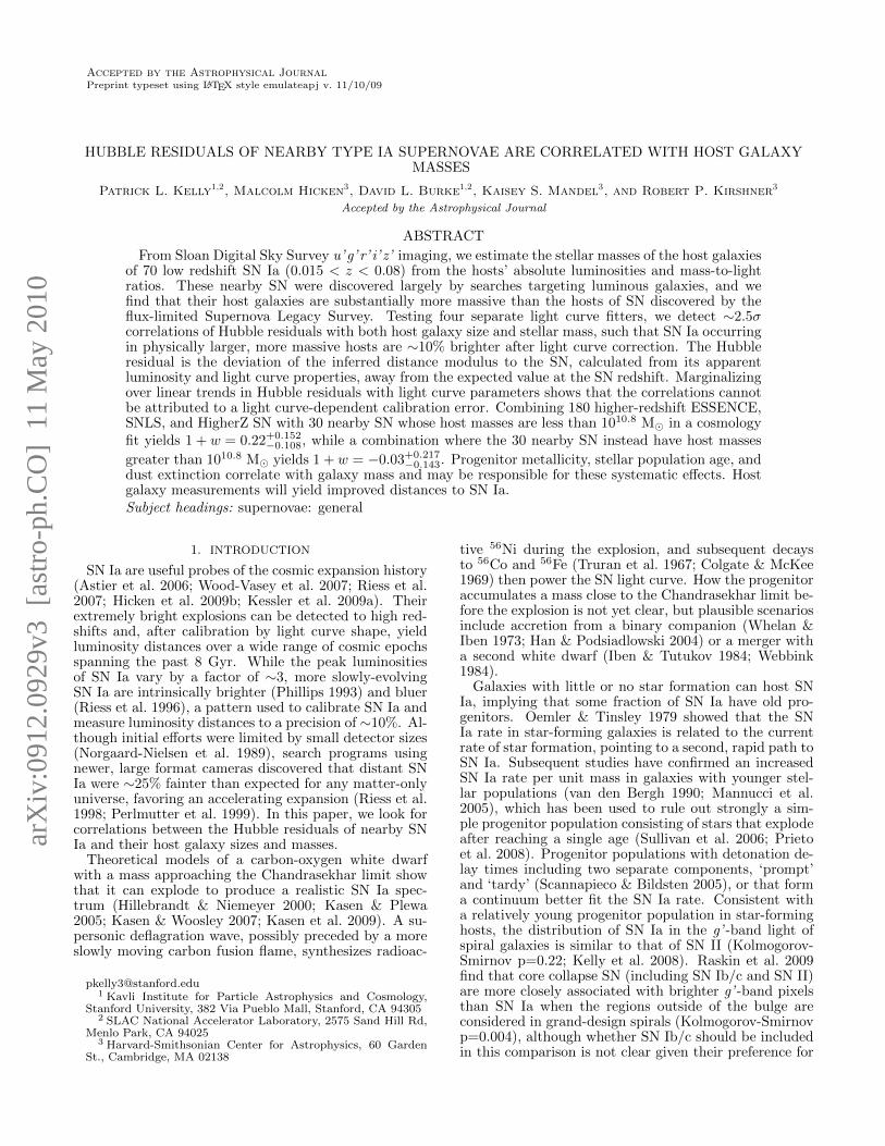
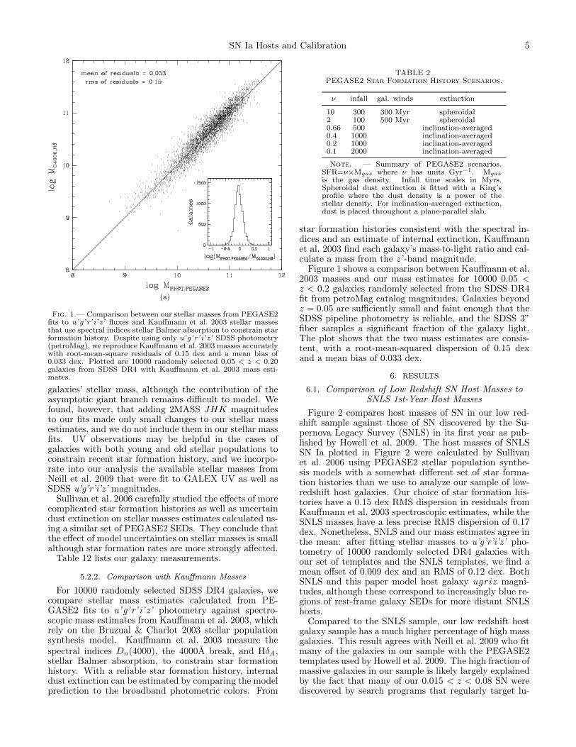
Fig. 1.— Comparison between our stellar masses from PEGASE2fits to u’g’r’ i’ z’ fluxes and Kauffmann et al. 2003 stellar massesthat use spectral indices stellar Balmer absorption to constrain starformation history. Despite using only u’g’r’ i’ z’ SDSS photometry(petroMag), we reproduce Kauffmann et al. 2003 masses accuratelywith root-mean-square residuals of 0.15 dex and a mean bias of0.033 dex. Plotted are 10000 randomly selected 0.05 < z < 0.20galaxies from SDSS DR4 with Kauffmann et al. 2003 mass esti-mates.

galaxies’ stellar mass, although the contribution of theasymptotic giant branch remains difficult to model. Wefound, however, that adding 2MASS JHK magnitudesto our fits made only small changes to our stellar massestimates, and we do not include them in our stellar massfits. UV observations may be helpful in the cases ofgalaxies with both young and old stellar populations toconstrain recent star formation history, and we incorpo-rate into our analysis the available stellar masses fromNeill et al. 2009 that were fit to GALEX UV as well asSDSS u’g’r’i’z’ magnitudes.

Sullivan et al. 2006 carefully studied the effects of morecomplicated star formation histories as well as uncertaindust extinction on stellar masses estimates calculated us-ing a similar set of PEGASE2 SEDs. They conclude thatthe effect of model uncertainties on stellar masses is smallalthough star formation rates are more strongly affected.

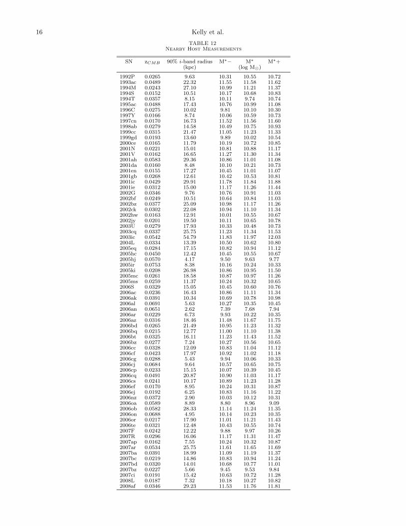
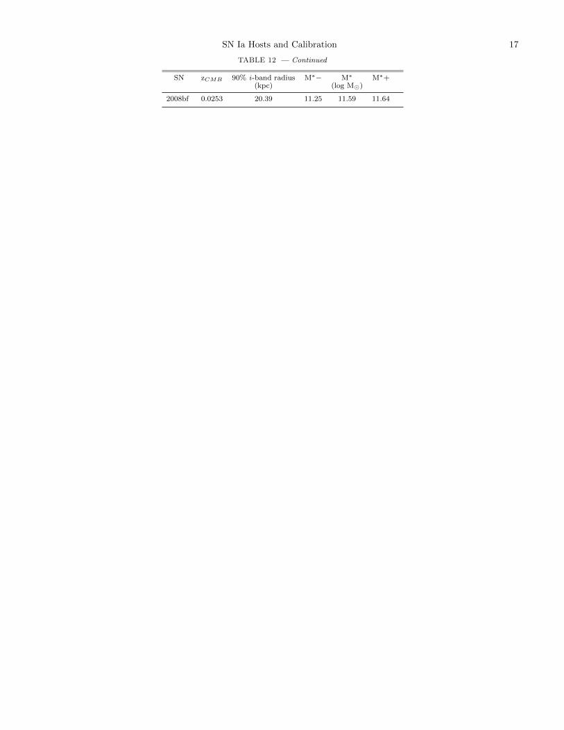
Table 12 lists our galaxy measurements.

5.2.2. Comparison with Kauffmann Masses

For 10000 randomly selected SDSS DR4 galaxies, wecompare stellar mass estimates calculated from PE-GASE2 fits to u’g’ r’ i’ z’ photometry against spectro-scopic mass estimates from Kauffmann et al. 2003, whichrely on the Bruzual & Charlot 2003 stellar populationsynthesis model. Kauffmann et al. 2003 measure thespectral indices Dn(4000), the 4000A break, and HδA,stellar Balmer absorption, to constrain star formationhistory. With a reliable star formation history, internaldust extinction can be estimated by comparing the modelprediction to the broadband photometric colors. From

TABLE 2PEGASE2 Star Formation History Scenarios.

ν infall gal. winds extinction

10 300 300 Myr spheroidal2 100 500 Myr spheroidal0.66 500 inclination-averaged0.4 1000 inclination-averaged0.2 1000 inclination-averaged0.1 2000 inclination-averaged

Note. — Summary of PEGASE2 scenarios.SFR=ν×Mgas where ν has units Gyr−1. Mgasis the gas density. Infall time scales in Myrs.Spheroidal dust extinction is fitted with a King’sprofile where the dust density is a power of thestellar density. For inclination-averaged extinction,dust is placed throughout a plane-parallel slab.

star formation histories consistent with the spectral in-dices and an estimate of internal extinction, Kauffmannet al. 2003 find each galaxy’s mass-to-light ratio and cal-culate a mass from the z’ -band magnitude.

Figure 1 shows a comparison between Kauffmann et al.2003 masses and our mass estimates for 10000 0.05 <z < 0.2 galaxies randomly selected from the SDSS DR4fit from petroMag catalog magnitudes. Galaxies beyondz = 0.05 are sufficiently small and faint enough that theSDSS pipeline photometry is reliable, and the SDSS 3”fiber samples a significant fraction of the galaxy light.The plot shows that the two mass estimates are consis-tent, with a root-mean-squared dispersion of 0.15 dexand a mean bias of 0.033 dex.

6. RESULTS

6.1. Comparison of Low Redshift SN Host Masses toSNLS 1st-Year Host Masses

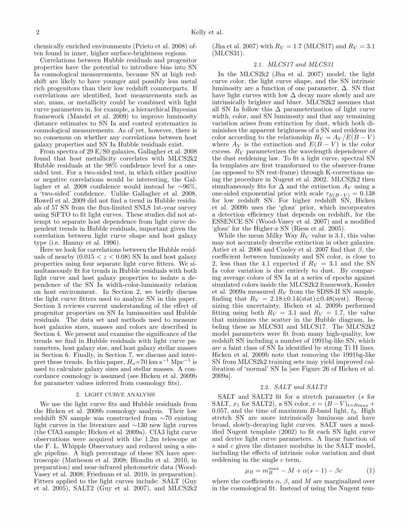
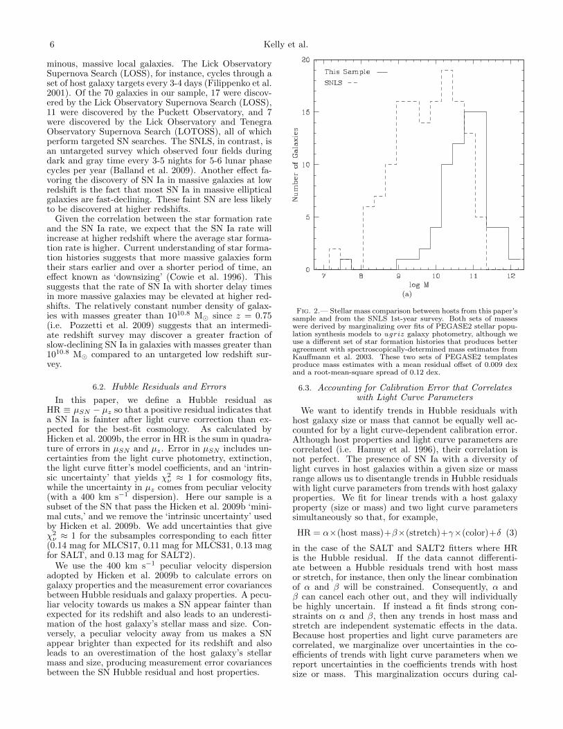
Figure 2 compares host masses of SN in our low red-shift sample against those of SN discovered by the Su-pernova Legacy Survey (SNLS) in its first year as pub-lished by Howell et al. 2009. The host masses of SNLSSN Ia plotted in Figure 2 were calculated by Sullivanet al. 2006 using PEGASE2 stellar population synthe-sis models with a somewhat different set of star forma-tion histories than we use to analyze our sample of low-redshift host galaxies. Our choice of star formation his-tories have a 0.15 dex RMS dispersion in residuals fromKauffmann et al. 2003 spectroscopic estimates, while theSNLS masses have a less precise RMS dispersion of 0.17dex. Nonetheless, SNLS and our mass estimates agree inthe mean: after fitting stellar masses to u’g’r’i’z’ pho-tometry of 10000 randomly selected DR4 galaxies withour set of templates and the SNLS templates, we find amean offset of 0.009 dex and an RMS of 0.12 dex. BothSNLS and this paper model host galaxy ugriz magni-tudes, although these correspond to increasingly blue re-gions of rest-frame galaxy SEDs for more distant SNLShosts.

Compared to the SNLS sample, our low redshift hostgalaxy sample has a much higher percentage of high massgalaxies. This result agrees with Neill et al. 2009 who fitmany of the galaxies in our sample with the PEGASE2templates used by Howell et al. 2009. The high fraction ofmassive galaxies in our sample is likely largely explainedby the fact that many of our 0.015 < z < 0.08 SN werediscovered by search programs that regularly target lu-

6 Kelly et al.

minous, massive local galaxies. The Lick ObservatorySupernova Search (LOSS), for instance, cycles through aset of host galaxy targets every 3-4 days (Filippenko et al.2001). Of the 70 galaxies in our sample, 17 were discov-ered by the Lick Observatory Supernova Search (LOSS),11 were discovered by the Puckett Observatory, and 7were discovered by the Lick Observatory and TenegraObservatory Supernova Search (LOTOSS), all of whichperform targeted SN searches. The SNLS, in contrast, isan untargeted survey which observed four fields duringdark and gray time every 3-5 nights for 5-6 lunar phasecycles per year (Balland et al. 2009). Another effect fa-voring the discovery of SN Ia in massive galaxies at lowredshift is the fact that most SN Ia in massive ellipticalgalaxies are fast-declining. These faint SN are less likelyto be discovered at higher redshifts.

Given the correlation between the star formation rateand the SN Ia rate, we expect that the SN Ia rate willincrease at higher redshift where the average star forma-tion rate is higher. Current understanding of star forma-tion histories suggests that more massive galaxies formtheir stars earlier and over a shorter period of time, aneffect known as ‘downsizing’ (Cowie et al. 1996). Thissuggests that the rate of SN Ia with shorter delay timesin more massive galaxies may be elevated at higher red-shifts. The relatively constant number density of galax-ies with masses greater than 1010.8 M� since z = 0.75(i.e. Pozzetti et al. 2009) suggests that an intermedi-ate redshift survey may discover a greater fraction ofslow-declining SN Ia in galaxies with masses greater than1010.8 M� compared to an untargeted low redshift sur-vey.

6.2. Hubble Residuals and Errors

In this paper, we define a Hubble residual asHR ≡ µSN − µz so that a positive residual indicates thata SN Ia is fainter after light curve correction than ex-pected for the best-fit cosmology. As calculated byHicken et al. 2009b, the error in HR is the sum in quadra-ture of errors in µSN and µz. Error in µSN includes un-certainties from the light curve photometry, extinction,the light curve fitter’s model coefficients, and an ‘intrin-sic uncertainty’ that yields χ2

ν ≈ 1 for cosmology fits,while the uncertainty in µz comes from peculiar velocity(with a 400 km s−1 dispersion). Here our sample is asubset of the SN that pass the Hicken et al. 2009b ‘mini-mal cuts,’ and we remove the ‘intrinsic uncertainty’ usedby Hicken et al. 2009b. We add uncertainties that giveχ2ν ≈ 1 for the subsamples corresponding to each fitter

(0.14 mag for MLCS17, 0.11 mag for MLCS31, 0.13 magfor SALT, and 0.13 mag for SALT2).

We use the 400 km s−1 peculiar velocity dispersionadopted by Hicken et al. 2009b to calculate errors ongalaxy properties and the measurement error covariancesbetween Hubble residuals and galaxy properties. A pecu-liar velocity towards us makes a SN appear fainter thanexpected for its redshift and also leads to an underesti-mation of the host galaxy’s stellar mass and size. Con-versely, a peculiar velocity away from us makes a SNappear brighter than expected for its redshift and alsoleads to an overestimation of the host galaxy’s stellarmass and size, producing measurement error covariancesbetween the SN Hubble residual and host properties.

(a)

Fig. 2.— Stellar mass comparison between hosts from this paper’ssample and from the SNLS 1st-year survey. Both sets of masseswere derived by marginalizing over fits of PEGASE2 stellar popu-lation synthesis models to ugriz galaxy photometry, although weuse a different set of star formation histories that produces betteragreement with spectroscopically-determined mass estimates fromKauffmann et al. 2003. These two sets of PEGASE2 templatesproduce mass estimates with a mean residual offset of 0.009 dexand a root-mean-square spread of 0.12 dex.

6.3. Accounting for Calibration Error that Correlateswith Light Curve Parameters

We want to identify trends in Hubble residuals withhost galaxy size or mass that cannot be equally well ac-counted for by a light curve-dependent calibration error.Although host properties and light curve parameters arecorrelated (i.e. Hamuy et al. 1996), their correlation isnot perfect. The presence of SN Ia with a diversity oflight curves in host galaxies within a given size or massrange allows us to disentangle trends in Hubble residualswith light curve parameters from trends with host galaxyproperties. We fit for linear trends with a host galaxyproperty (size or mass) and two light curve parameterssimultaneously so that, for example,

HR = α×(host mass)+β×(stretch)+γ×(color)+δ (3)

in the case of the SALT and SALT2 fitters where HRis the Hubble residual. If the data cannot differenti-ate between a Hubble residuals trend with host massor stretch, for instance, then only the linear combinationof α and β will be constrained. Consequently, α andβ can cancel each other out, and they will individuallybe highly uncertain. If instead a fit finds strong con-straints on α and β, then any trends in host mass andstretch are independent systematic effects in the data.Because host properties and light curve parameters arecorrelated, we marginalize over uncertainties in the co-efficients of trends with light curve parameters when wereport uncertainties in the coefficients trends with hostsize or mass. This marginalization occurs during cal-

SN Ia Hosts and Calibration 7

(a) (b)

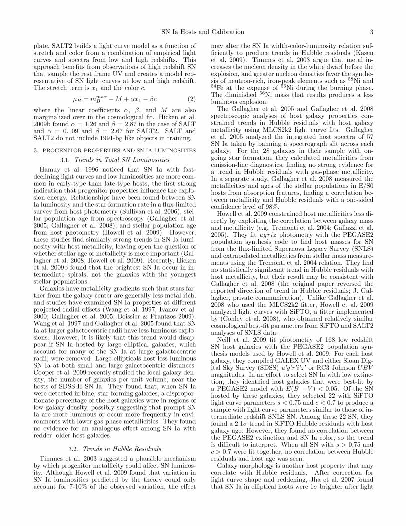
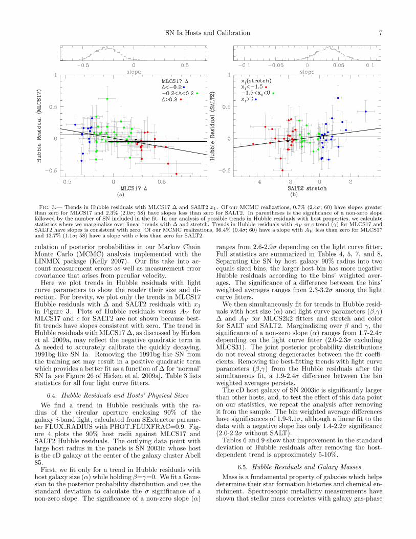
Fig. 3.— Trends in Hubble residuals with MLCS17 ∆ and SALT2 x1. Of our MCMC realizations, 0.7% (2.4σ; 60) have slopes greaterthan zero for MLCS17 and 2.3% (2.0σ; 58) have slopes less than zero for SALT2. In parentheses is the significance of a non-zero slopefollowed by the number of SN included in the fit. In our analysis of possible trends in Hubble residuals with host properties, we calculatestatistics where we marginalize over linear trends with ∆ and stretch. Trends in Hubble residuals with AV or c trend (γ) for MLCS17 andSALT2 have slopes is consistent with zero. Of our MCMC realizations, 36.4% (0.4σ; 60) have a slope with AV less than zero for MLCS17and 13.7% (1.1σ; 58) have a slope with c less than zero for SALT2.

culation of posterior probabilities in our Markov ChainMonte Carlo (MCMC) analysis implemented with theLINMIX package (Kelly 2007). Our fits take into ac-count measurement errors as well as measurement errorcovariance that arises from peculiar velocity.

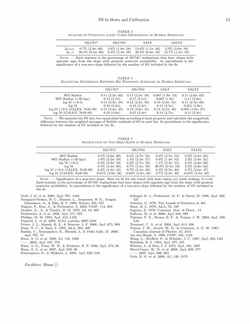
Here we plot trends in Hubble residuals with lightcurve parameters to show the reader their size and di-rection. For brevity, we plot only the trends in MLCS17Hubble residuals with ∆ and SALT2 residuals with x1in Figure 3. Plots of Hubble residuals versus AV forMLCS17 and c for SALT2 are not shown because best-fit trends have slopes consistent with zero. The trend inHubble residuals with MLCS17 ∆, as discussed by Hickenet al. 2009a, may reflect the negative quadratic term in∆ needed to accurately calibrate the quickly decaying,1991bg-like SN Ia. Removing the 1991bg-like SN fromthe training set may result in a positive quadratic termwhich provides a better fit as a function of ∆ for ‘normal’SN Ia [see Figure 26 of Hicken et al. 2009a]. Table 3 listsstatistics for all four light curve fitters.

6.4. Hubble Residuals and Hosts’ Physical Sizes

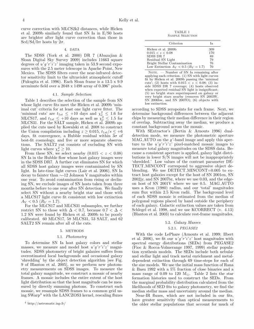
We find a trend in Hubble residuals with the ra-dius of the circular aperture enclosing 90% of thegalaxy i-band light, calculated from SExtractor parame-ter FLUX RADIUS with PHOT FLUXFRAC=0.9. Fig-ure 4 plots the 90% host radii against MLCS17 andSALT2 Hubble residuals. The outlying data point withlarge host radius in the panels is SN 2003ic whose hostis the cD galaxy at the center of the galaxy cluster Abell85.

First, we fit only for a trend in Hubble residuals withhost galaxy size (α) while holding β=γ=0. We fit a Gaus-sian to the posterior probability distribution and use thestandard deviation to calculate the σ significance of anon-zero slope. The significance of a non-zero slope (α)

ranges from 2.6-2.9σ depending on the light curve fitter.Full statistics are summarized in Tables 4, 5, 7, and 8.Separating the SN by host galaxy 90% radius into twoequals-sized bins, the larger-host bin has more negativeHubble residuals according to the bins’ weighted aver-ages. The significance of a difference between the bins’weighted averages ranges from 2.3-3.2σ among the lightcurve fitters.

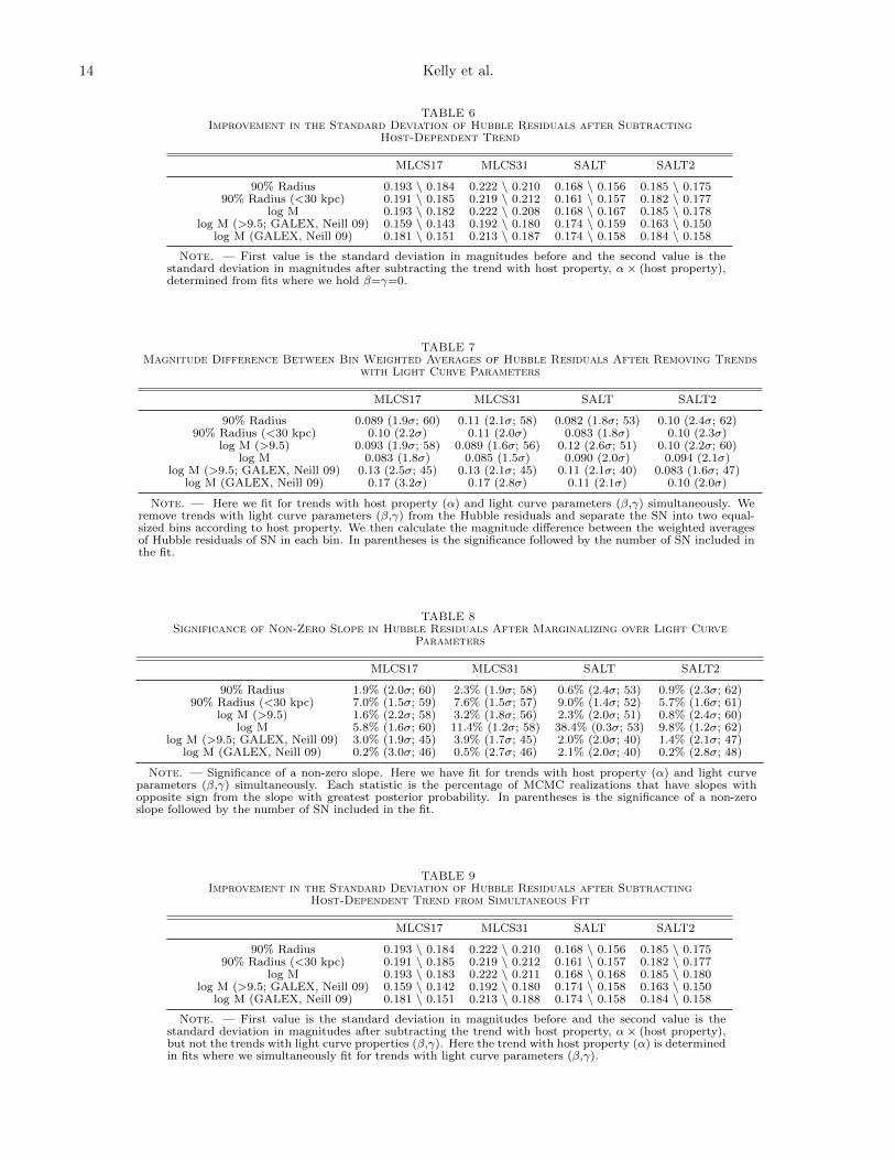
We then simultaneously fit for trends in Hubble resid-uals with host size (α) and light curve parameters (β,γ)∆ and AV for MLCS2k2 fitters and stretch and colorfor SALT and SALT2. Marginalizing over β and γ, thesignificance of a non-zero slope (α) ranges from 1.7-2.4σdepending on the light curve fitter (2.0-2.3σ excludingMLCS31). The joint posterior probability distributionsdo not reveal strong degeneracies between the fit coeffi-cients. Removing the best-fitting trends with light curveparameters (β,γ) from the Hubble residuals after thesimultaneous fit, a 1.9-2.4σ difference between the binweighted averages persists.

The cD host galaxy of SN 2003ic is significantly largerthan other hosts, and, to test the effect of this data pointon our statistics, we repeat the analysis after removingit from the sample. The bin weighted average differenceshave significances of 1.9-3.1σ, although a linear fit to thedata with a negative slope has only 1.4-2.2σ significance(2.0-2.2σ without SALT).

Tables 6 and 9 show that improvement in the standarddeviation of Hubble residuals after removing the host-dependent trend is approximately 5-10%.

6.5. Hubble Residuals and Galaxy Masses

Mass is a fundamental property of galaxies which helpsdetermine their star formation histories and chemical en-richment. Spectroscopic metallicity measurements haveshown that stellar mass correlates with galaxy gas-phase

8 Kelly et al.

(a) (b)

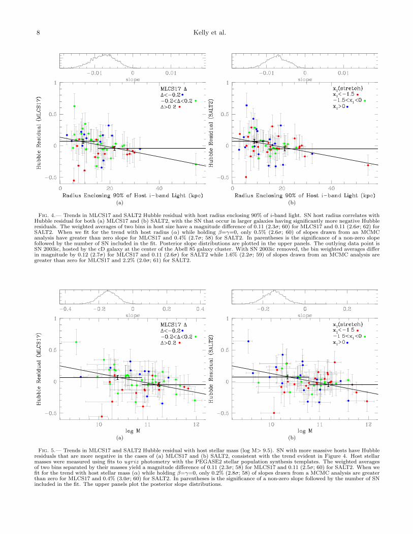
Fig. 4.— Trends in MLCS17 and SALT2 Hubble residual with host radius enclosing 90% of i-band light. SN host radius correlates withHubble residual for both (a) MLCS17 and (b) SALT2, with the SN that occur in larger galaxies having significantly more negative Hubbleresiduals. The weighted averages of two bins in host size have a magnitude difference of 0.11 (2.3σ; 60) for MLCS17 and 0.11 (2.6σ; 62) forSALT2. When we fit for the trend with host radius (α) while holding β=γ=0, only 0.5% (2.6σ; 60) of slopes drawn from an MCMCanalysis have greater than zero slope for MLCS17 and 0.4% (2.7σ; 58) for SALT2. In parentheses is the significance of a non-zero slopefollowed by the number of SN included in the fit. Posterior slope distributions are plotted in the upper panels. The outlying data point isSN 2003ic, hosted by the cD galaxy at the center of the Abell 85 galaxy cluster. With SN 2003ic removed, the bin weighted averages differin magnitude by 0.12 (2.7σ) for MLCS17 and 0.11 (2.6σ) for SALT2 while 1.6% (2.2σ; 59) of slopes drawn from an MCMC analysis aregreater than zero for MLCS17 and 2.2% (2.0σ; 61) for SALT2.

(a) (b)

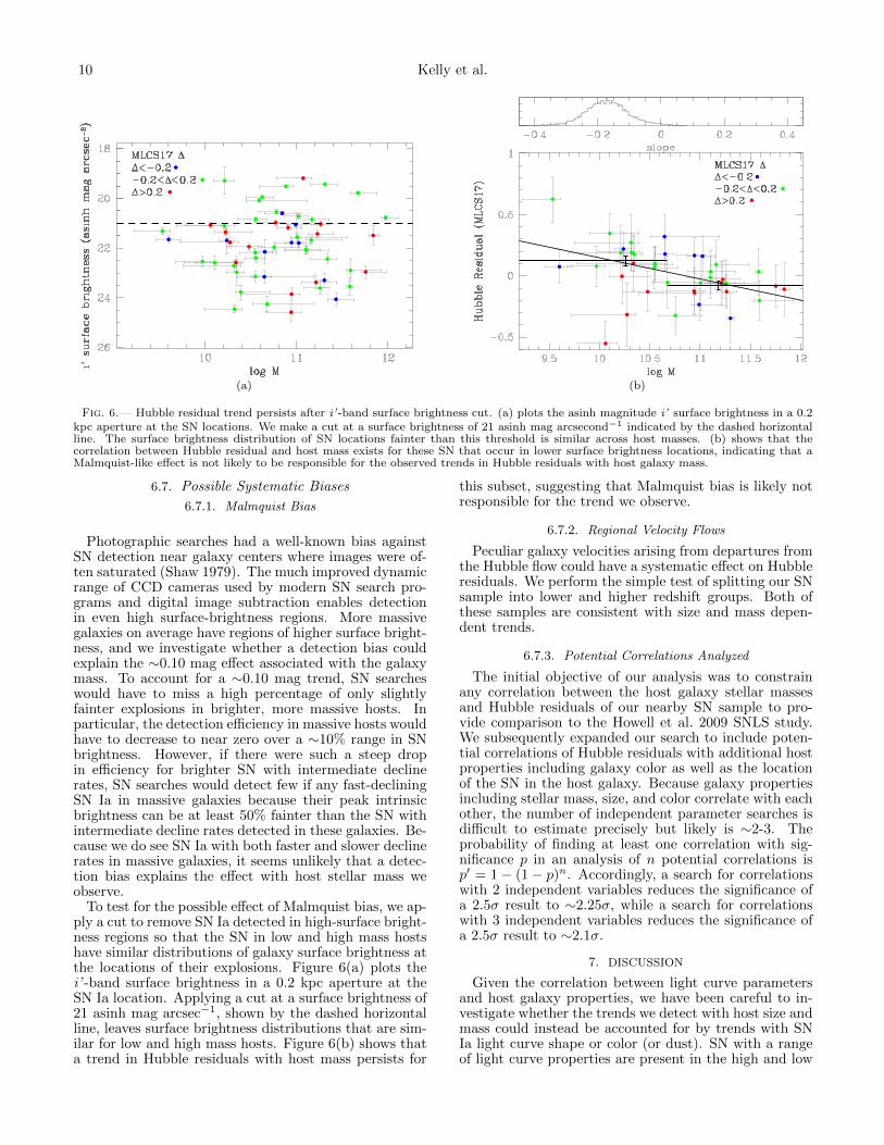
Fig. 5.— Trends in MLCS17 and SALT2 Hubble residual with host stellar mass (log M> 9.5). SN with more massive hosts have Hubbleresiduals that are more negative in the cases of (a) MLCS17 and (b) SALT2, consistent with the trend evident in Figure 4. Host stellarmasses were measured using fits to ugriz photometry with the PEGASE2 stellar population synthesis templates. The weighted averagesof two bins separated by their masses yield a magnitude difference of 0.11 (2.3σ; 58) for MLCS17 and 0.11 (2.5σ; 60) for SALT2. When wefit for the trend with host stellar mass (α) while holding β=γ=0, only 0.2% (2.8σ; 58) of slopes drawn from a MCMC analysis are greaterthan zero for MLCS17 and 0.4% (3.0σ; 60) for SALT2. In parentheses is the significance of a non-zero slope followed by the number of SNincluded in the fit. The upper panels plot the posterior slope distributions.

SN Ia Hosts and Calibration 9

(Tremonti et al. 2004) and stellar (Gallazzi et al. 2005)metal content, reflecting the fact that it is easier for met-als to escape from the shallower gravitational potentialsof less massive galaxies. As seen in Figure 2, only 2 ofour SN host galaxies have masses less than 109.5 M�.Timmes et al. 2003 argue that the effect of metallicityon SN Ia luminosity depends non-linearly on the pro-genitor’s metallicity, which might mean that any effecton Hubble residuals would only become strong for SNIa in massive galaxies. We restrict our sample for ourprimary analysis to SN with galaxy hosts more massivethan 109.5 M� where we have a sufficient number of SNwith massive hosts to constrain any systematic trend.

We plot galaxy stellar mass against Hubble residuals inFigure 5 for the MLCS17 and SALT2 light curve fitters,excluding the 2 SN with the least massive hosts. Tables 4,5, 7, and 8 summarize all of our statistical tests. First, wefit only for a trend in Hubble residuals with host galaxymass (α) while holding β=γ=0. The significance of anon-zero slope (α) ranges from 2.3-2.8σ depending onthe light curve fitter. Separating the SN by host galaxymass into two equal-sized bins, the more massive hostbin has more negative Hubble residuals according to thebins’ weighted averages. The significance of a differencebetween the bins’ weighted averages ranges from 2.2-2.8σamong the light curve fitters.

We then simultaneously fit for trends in Hubble resid-uals with host mass (α) and light curve parameters (β,γ)∆ and AV for MLCS2k2 fitters and stretch and color forSALT and SALT2. Marginalizing over β and γ, the sig-nificance of a non-zero slope (α) ranges from 2.0-2.6σdepending on the light curve fitter. The joint poste-rior probability distributions do not reveal strong degen-eracies between the fit coefficients. Removing the best-fitting trends with light curve parameters (β,γ) from theHubble residuals after the simultaneous fit, a 1.6-2.6σdifference between the bin weighted averages persists.

Tables 6 and 9 show that the reduction in the standarddeviation of Hubble residuals after removing the host-dependent trend is approximately 5-10%.

6.5.1. Neill et al. 2009 Masses

We now repeat the analyses using stellar mass esti-mates from Neill et al. 2009, which were fit using GALEXUV measurements in addition to SDSS u’g’ r’ i’ z’ mag-nitudes. Because each Neill et al. 2009 host galaxy isrequired to have UV as well as optical measurements,Neill et al. 2009 measured masses for only 49 of the 70SN in our sample with MLCS17 AV < 0.5. Fitting onlyfor a trend in Hubble residuals with host galaxy mass(α) while holding β=γ=0, the significance of a non-zeroslope (α) ranges from 2.3-2.7σ depending on the lightcurve fitter. The significance of a difference between thebins’ weighted averages ranges from 1.8-3.2σ among thelight curve fitters.

Simultaneously fitting for and marginalizing over lineartrends (β,γ) with light curve parameters, the significanceof a non-zero slope (α) is 1.9σ for all light curve fitters.The joint posterior probability distributions do not revealstrong degeneracies between the fit coefficients. Remov-ing the best-fitting trends with light curve parameters(β,γ) from the Hubble residuals after the simultaneousfit, a 1.6-2.5σ (2.1-2.5σ without SALT2) difference be-tween the bin weighted averages remains.

Tables 6 and 9 show the improvement in the standarddeviation of Hubble residuals after removing the host-dependent trend. This results in improvements of up to15% in standard deviation.

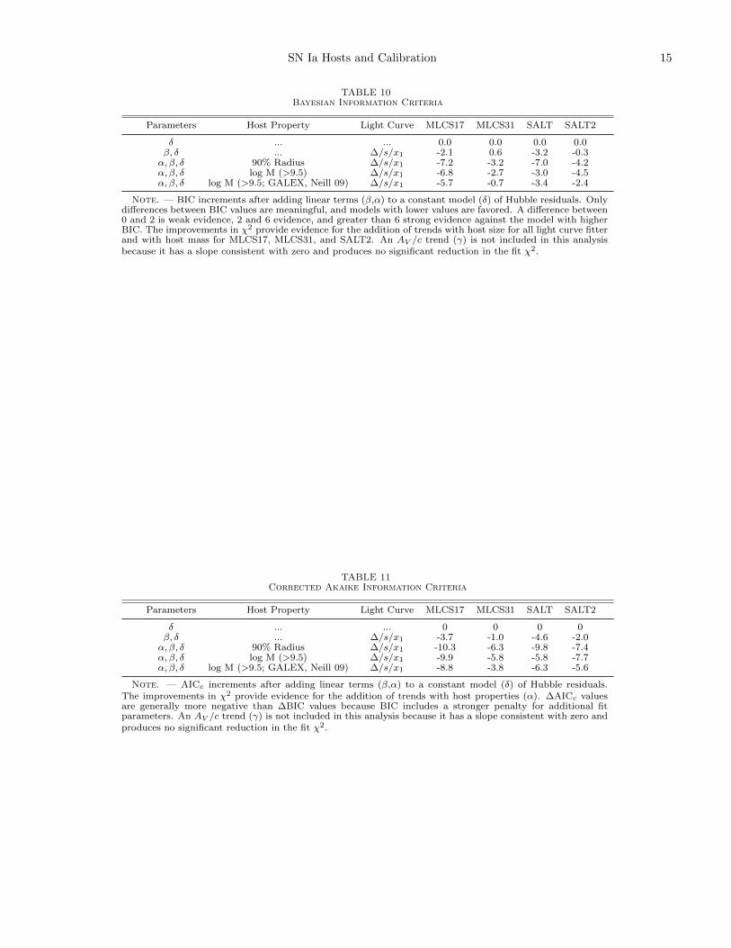
6.6. Information Criteria

The Bayesian information criterion (BIC) and theAkaike information criterion (AIC) help to evaluatewhether an additional model parameter can be justifiedby the improvement it produces in the χ2 goodness-of-fit statistic. BIC derives from an approximation to theBayes factor, the ratio of the probabilities of two modelsgiven equal prior probability. For any two prospectivemodels, the model with the lower value of BIC is thepreferred one. With Gaussian errors, the BIC (Schwarz1978) is given as,

BIC = χ2 + k lnN (4)

where k is the number of parameters and N isthe number of data points in the fit. A compari-son can be made between two models by computing∆BIC = ∆χ2 + ∆k lnN . The AIC (Akaike 1974) usesKullback-Leibler information entropy as a basis to com-pare different models of a given data set. The AICc is aversion of the AIC corrected for small data sets (Sugiura1978),

AICc = χ2 + 2k +2k(k + 1)

N − k − 1(5)

where k is the number of parameters andN is the numberof data points used in fit. A decrease of 2 in the infor-mation criterion is positive evidence against the modelwith higher information criterion, while a decrease of 6is strong positive evidence against the model with largervalue (e.g. Kass & Raftery 1995, Mukherjee et al. 1998).To calculate these statistics, we first add an ‘intrinsic un-certainty’ in quadrature to the Hubble residual error oneach SN so that χ2

ν = 1 for a fit with no trends. Wecalculate the BIC and AICc for three separate models:no trend (δ), a trend with light curve shape parameter(β, δ), and trends with light curve shape parameter andhost galaxy property (α, β, δ). Only differences in in-formation criteria are significant, and Tables 10 and 11list the change in the information criteria relative to themodel with no trend (δ). An AV /c trend (γ) is not in-cluded because its slope is consistent with zero and itsinclusion results in no significant reduction in the fit χ2.

We are interested in the changes in the BIC and AICcafter adding a host dependent trend (α) to a model thatalready includes a trend with light curve shape (β, δ).For all light curve fitters, an added trend with host sizeproduces ∆BIC < −2, providing evidence in favor ofthe additional trend. For trends with host stellar mass,∆BIC < −2 except for SALT. MLCS17 and SALT2 have∆BIC < −2 for Neill et al. 2009 stellar masses. Only if∆BIC > 2 would there be evidence against adding a hostdependent term, and in no case is ∆BIC > 2. ∆AICc ismore negative in all cases than ∆BIC because BIC hasa stronger penalty for each additional parameter. In thecases of all trends and all light curve fitters, ∆AICc < −2and largely is less than -4, providing moderate to strongpositive evidence for a host dependent term.

10 Kelly et al.

(a) (b)

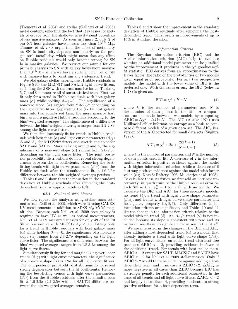
Fig. 6.— Hubble residual trend persists after i’ -band surface brightness cut. (a) plots the asinh magnitude i’ surface brightness in a 0.2kpc aperture at the SN locations. We make a cut at a surface brightness of 21 asinh mag arcsecond−1 indicated by the dashed horizontalline. The surface brightness distribution of SN locations fainter than this threshold is similar across host masses. (b) shows that thecorrelation between Hubble residual and host mass exists for these SN that occur in lower surface brightness locations, indicating that aMalmquist-like effect is not likely to be responsible for the observed trends in Hubble residuals with host galaxy mass.

6.7. Possible Systematic Biases

6.7.1. Malmquist Bias

Photographic searches had a well-known bias againstSN detection near galaxy centers where images were of-ten saturated (Shaw 1979). The much improved dynamicrange of CCD cameras used by modern SN search pro-grams and digital image subtraction enables detectionin even high surface-brightness regions. More massivegalaxies on average have regions of higher surface bright-ness, and we investigate whether a detection bias couldexplain the ∼0.10 mag effect associated with the galaxymass. To account for a ∼0.10 mag trend, SN searcheswould have to miss a high percentage of only slightlyfainter explosions in brighter, more massive hosts. Inparticular, the detection efficiency in massive hosts wouldhave to decrease to near zero over a ∼10% range in SNbrightness. However, if there were such a steep dropin efficiency for brighter SN with intermediate declinerates, SN searches would detect few if any fast-decliningSN Ia in massive galaxies because their peak intrinsicbrightness can be at least 50% fainter than the SN withintermediate decline rates detected in these galaxies. Be-cause we do see SN Ia with both faster and slower declinerates in massive galaxies, it seems unlikely that a detec-tion bias explains the effect with host stellar mass weobserve.

To test for the possible effect of Malmquist bias, we ap-ply a cut to remove SN Ia detected in high-surface bright-ness regions so that the SN in low and high mass hostshave similar distributions of galaxy surface brightness atthe locations of their explosions. Figure 6(a) plots thei’ -band surface brightness in a 0.2 kpc aperture at theSN Ia location. Applying a cut at a surface brightness of21 asinh mag arcsec−1, shown by the dashed horizontalline, leaves surface brightness distributions that are sim-ilar for low and high mass hosts. Figure 6(b) shows thata trend in Hubble residuals with host mass persists for

this subset, suggesting that Malmquist bias is likely notresponsible for the trend we observe.

6.7.2. Regional Velocity Flows

Peculiar galaxy velocities arising from departures fromthe Hubble flow could have a systematic effect on Hubbleresiduals. We perform the simple test of splitting our SNsample into lower and higher redshift groups. Both ofthese samples are consistent with size and mass depen-dent trends.

6.7.3. Potential Correlations Analyzed

The initial objective of our analysis was to constrainany correlation between the host galaxy stellar massesand Hubble residuals of our nearby SN sample to pro-vide comparison to the Howell et al. 2009 SNLS study.We subsequently expanded our search to include poten-tial correlations of Hubble residuals with additional hostproperties including galaxy color as well as the locationof the SN in the host galaxy. Because galaxy propertiesincluding stellar mass, size, and color correlate with eachother, the number of independent parameter searches isdifficult to estimate precisely but likely is ∼2-3. Theprobability of finding at least one correlation with sig-nificance p in an analysis of n potential correlations isp′ = 1 − (1 − p)n. Accordingly, a search for correlationswith 2 independent variables reduces the significance ofa 2.5σ result to ∼2.25σ, while a search for correlationswith 3 independent variables reduces the significance ofa 2.5σ result to ∼2.1σ.

7. DISCUSSION

Given the correlation between light curve parametersand host galaxy properties, we have been careful to in-vestigate whether the trends we detect with host size andmass could instead be accounted for by trends with SNIa light curve shape or color (or dust). SN with a rangeof light curve properties are present in the high and low

SN Ia Hosts and Calibration 11

mass ends of the host galaxy distribution, and this allowsus to disentangle potential effects of size, mass, and lightcurve parameters. By simultaneously fitting for and thenmarginalizing over trends with light curve parameters inour fits for host-dependent trends, we have shown thatcalibration errors that correlate with light curve prop-erties do not account for the trends we find in Hubbleresiduals with host galaxy size and mass.

Host galaxy metallicity, stellar age, and extinction bydust correlate with galaxy mass and may be factors re-sponsible for the variation we observe in the SN Ia width-color-luminosity relation. According to the Timmes et al.2003 model, the effect of metallicity on SN Ia lumi-nosities depends non-linearly on metallicity and wouldbe strongest at the high metallicities of the massivegalaxies in our sample. Kasen et al. 2009 included theTimmes et al. 2003 effect in SN Ia simulations and foundthat increased metallicity would alter the SN Ia width-luminosity relation so that SN Ia with intermediate toslow decline rates would be intrinsically brighter afterlight curve correction. Such a correction would be con-sistent with the direction of the trend we see in Hubbleresiduals with increasing host masses, at least for SNwith slower decay rates. Kasen et al. 2009 did not ac-count for the possible effects of metals on the dynamicsof the explosion, or on the white dwarf’s structure. Wenote that an interesting feature of Figure 4 is the appar-ent lack of a strong trend in the Hubble residuals withradius for SN Ia in host galaxies with sizes greater than15 kpc.

That the hosts of our low redshift SN Ia are substan-tially more massive than hosts of 0.2 < z < 0.75 SNLSSN helps to interpret existing studies of Hubble resid-uals and host galaxy properties. Figure 2 shows thatHowell et al. 2009, analyzing SNLS SN, fit for a lineartrend in Hubble residuals over a much larger range of hostmasses than we do and have comparatively few galaxieswith masses greater than 1011 M�, perhaps helping toexplain the fact that they found no strong trend in Hub-ble residuals with host metallicity. Gallagher et al. 2005studied SN Ia in star-forming and therefore likely lessmassive low redshift galaxies, finding no significant trendin Hubble residuals with host metallicity. Gallagher et al.2008, however, studied low redshift E/S0 galaxies, whichare likely similar to the more massive hosts in our sample(four hosts overlap with our sample), and found a 98%confidence in a trend in host metallicity.

Both Gallagher et al. 2008 and Howell et al. 2009 favortrends (although the Howell et al. 2009 trend only has1-σ significance) where galaxies with higher metallicitieshost SN that are brighter than expected. If the moremassive galaxies in our sample have higher metallicities,the direction of the trends we find agrees with the direc-tion of the trend in Hubble residuals with host metallic-ity found by Gallagher et al. 2008. The Neill et al. 2009trend in Hubble residuals with host age exists only in asubset of SN whose hosts have low extinction but whoselight curve colors are not necessarily consistent with lowextinction, making comparison with our trend difficult.

While we could in theory use an empirical mass-metallicity relation to test directly for the effect of metal-licity in our sample following Howell et al. 2009 and Neillet al. 2009, it is not clear which mass-metallicity rela-tion is appropriate. The fact that SN Ia progenitors are

likely to be younger in later-type hosts may mean thattheir metallicities are similar to the gas-phase metallic-ity while SN Ia progenitors in older, early-type galaxiesmay track the stellar metallicity. The slope of mass-metallicity relation also becomes flatter for galaxies withapproximately 1010.5 M�, making mass a less sensitiveproxy for metallicity.

7.1. Strong Cosmology Implications

Low redshift SN are essential to accurate constraintson the dark energy equation of state parameter, w, be-cause they anchor the redshift-distance relation and setthe expectation for the brightnesses of high redshift SNaccording to different cosmologies. The discovery thatthe universe is accelerating in its expansion originatedfrom the observation that high redshift SN Ia were fainterthan expected for a matter-only universe (Riess et al.1998; Perlmutter et al. 1999). Low redshift SN are alsoused to train the MLCS2k2 light fitters and consequentlyinfluence distance measurements to high redshift SN. AsFigure 2 demonstrates, only a small percentage of SN dis-covered by the SNLS flux-limited survey have host galaxymass greater than 1010.8 M�. However, half of the lowredshift sample has hosts more massive than 1010.8 M�,and this paper has shown that these SN have Hubbleresiduals that are on average more negative by ∼0.10mag.

To examine the sensitivity of the best-fitting valueof w to the host-dependent calibration error, we divideour sample into two sets according to whether the SNhost has a mass greater or less than 1010.8 M�. Us-ing the wfit cosmology fitter from the Supernova Anal-ysis package (Kessler et al. 2009b) and incorporatingbaryon acoustic oscillation (Eisenstein et al. 2005) andcosmic microwave background (Komatsu et al. 2009)measurements, the best-fitting values of w differ. Whenfit in combination with 180 higher-redshift ESSENCE,SNLS, and HigherZ SN, the 30 SN with lower masshosts yield 1 + w = 0.22+0.152

−0.108 while the 30 nearby SN

with higher mass hosts yield 1 + w = −0.03+0.217−0.143 from

MLCS17 measurements. The difference between the twoestimates of w is likely more significant than indicated bythe overlap between their constraints, because they in-clude 180 higher-redshift SN in common. The 30 nearbyhosts with masses less than 1010.8 M� in our sample aremore massive than a majority of SNLS host galaxies, sowe note that we have not constructed a sample of SNIa with hosts of similar masses across all redshifts. Thehost-dependent shift in w is greater than the statisticalerror on w and implies that host galaxy or progenitor-dependent effects have an unappreciated and strong in-fluence on even current SN cosmological estimates.

8. CONCLUSIONS AND SUMMARY

The hosts of our sample of 70 low redshift (0.015 <z < 0.08) SN are substantially more massive than hostsof the intermediate redshift (0.2 < z < 0.75) SNLS SN.In our sample, SN Ia that occur in larger, more massivegalaxies are ∼10% brighter than SN Ia found in smaller,less massive galaxies after light curve correction when wecalculate distance moduli using the MLCS17, MLCS31,SALT and SALT2 fitters. When we fit simultaneouslyfor trends with light curve parameters in addition to

12 Kelly et al.

host galaxy properties, we find that these host-dependenttrends in Hubble residuals cannot be accounted for bylight curve-dependent calibration error.

The variation in the SN Ia width-color-luminosity rela-tion with host size and mass implied by these trends mayreflect the correlation between galaxy mass and metallic-ity, increased average ages of progenitors in more massivehosts, or another environmental difference such as dustextinction. Sensitivity of SN Ia luminosities to progenitormetallicity may become greatest at the high metallicitiesfound in the most massive hosts in our sample (Timmeset al. 2003).

Nearby SN Ia detected by targeted searches should betreated carefully when included in cosmology fits becausetheir host galaxies are generally substantially more mas-sive than those of SN detected by flux-limited surveys athigher redshifts. The 30 nearby SN with host masses lessthan 1010.8 M� in our sample yield 1 + w = 0.22+0.152

−0.108while the set of 30 nearby SN with more massive hostsyield 1 + w = −0.03+0.217

−0.143 with MLCS17 distances whenfit in combination with 180 higher-redshift ESSENCE,SNLS, and HigherZ SN. By combining information fromhost galaxy measurements with light curve fits, distancesto SN Ia may be more accurately estimated and used tomeasure cosmological parameters with better control ofsystematics.

We would like to thank especially R. Romani, M. Blan-ton, A. von der Linden, S. Allen, A. Mantz, C. Zhang, M.Sako, B. Haussler, and C. Peng as well as D. Rapetti, B.

Holden, D. Applegate, M. Allen, P. Behroozi, O. Ilbert,S. Arnouts, and J. Gallagher. NSF grants AST0907903and AST0606772 as well as the U.S. Department of En-ergy contract DE-AC02-70SF00515 support research onSN at Harvard University.

Funding for the SDSS and SDSS-II has been providedby the Alfred P. Sloan Foundation, the Participating In-stitutions, the National Science Foundation, the U.S.Department of Energy, the National Aeronautics andSpace Administration, the Japanese Monbukagakusho,the Max Planck Society, and the Higher Education Fund-ing Council for England.

The SDSS is managed by the Astrophysical ResearchConsortium for the Participating Institutions. The Par-ticipating Institutions are the American Museum of Nat-ural History, Astrophysical Institute Potsdam, Univer-sity of Basel, Cambridge University, Case Western Re-serve University, University of Chicago, Drexel Univer-sity, Fermilab, the Institute for Advanced Study, theJapan Participation Group, Johns Hopkins University,the Joint Institute for Nuclear Astrophysics, the KavliInstitute for Particle Astrophysics and Cosmology, theKorean Scientist Group, the Chinese Academy of Sci-ences (LAMOST), Los Alamos National Laboratory, theMax-Planck-Institute for Astronomy (MPIA), the Max-Planck-Institute for Astrophysics (MPA), New MexicoState University, Ohio State University, University ofPittsburgh, University of Portsmouth, Princeton Uni-versity, the United States Naval Observatory, and theUniversity of Washington.

REFERENCES

Abazajian, K., & Sloan Digital Sky Survey, f. t. 2009, ApJS, 182,543

Akaike, H. 1974, IEEE T. Automat. Contr., 19, 716Arnouts, S., Cristiani, S., Moscardini, L., Matarrese, S., Lucchin,

F., Fontana, A., & Giallongo, E. 1999, MNRAS, 310, 540Astier, P. et al. 2006, A&A, 447, 31Balland, C. et al. 2009, A&A, 507, 85, 0909.3316Bertin, E., & Arnouts, S. 1996, A&AS, 117, 393Blanton, M. R. et al. 2003, AJ, 125, 2348——. 2005, AJ, 129, 2562Boissier, S., & Prantzos, N. 2009, A&A, 503, 137Bruzual, G., & Charlot, S. 2003, MNRAS, 344, 1000Colgate, S. A., & McKee, C. 1969, ApJ, 157, 623Conley, A., Carlberg, R. G., Guy, J., Howell, D. A., Jha, S.,

Riess, A. G., & Sullivan, M. 2007, ApJ, 664, L13Conley, A. et al. 2008, ApJ, 681, 482Cooper, M. C., Newman, J. A., & Yan, R. 2009, ApJ, 704, 687Cowie, L. L., Songaila, A., Hu, E. M., & Cohen, J. G. 1996, AJ,

112, 839Eisenstein, D. J. et al. 2005, ApJ, 633, 560Filippenko, A. V., Li, W. D., Treffers, R. R., & Modjaz, M. 2001,

in Astronomical Society of the Pacific Conference Series, Vol.246, IAU Colloq. 183: Small Telescope Astronomy on GlobalScales, ed. B. Paczynski, W.-P. Chen, & C. Lemme, 121–+

Fioc, M., & Rocca-Volmerange, B. 1997, A&A, 326, 950——. 1999, ArXiv e-prints, 9912.0179Fukugita, M., Ichikawa, T., Gunn, J. E., Doi, M., Shimasaku, K.,

& Schneider, D. P. 1996, AJ, 111, 1748Gallagher, J. S., Garnavich, P. M., Berlind, P., Challis, P., Jha,

S., & Kirshner, R. P. 2005, ApJ, 634, 210Gallagher, J. S., Garnavich, P. M., Caldwell, N., Kirshner, R. P.,

Jha, S. W., Li, W., Ganeshalingam, M., & Filippenko, A. V.2008, ApJ, 685, 752

Gallazzi, A., Charlot, S., Brinchmann, J., White, S. D. M., &Tremonti, C. A. 2005, MNRAS, 362, 41

Guy, J. et al. 2007, A&A, 466, 11

Guy, J., Astier, P., Nobili, S., Regnault, N., & Pain, R. 2005,A&A, 443, 781

Hamuy, M., Phillips, M. M., Suntzeff, N. B., Schommer, R. A.,Maza, J., & Aviles, R. 1996, AJ, 112, 2391

Han, Z., & Podsiadlowski, P. 2004, MNRAS, 350, 1301Hicken, M. et al. 2009a, ApJ, 700, 331Hicken, M., Wood-Vasey, W. M., Blondin, S., Challis, P., Jha, S.,

Kelly, P. L., Rest, A., & Kirshner, R. P. 2009b, ApJ, 700, 1097Hillebrandt, W., & Niemeyer, J. C. 2000, ARA&A, 38, 191Howell, D. A. et al. 2009, ApJ, 691, 661Iben, Jr., I., & Tutukov, A. V. 1984, ApJS, 54, 335Ilbert, O. et al. 2006, A&A, 457, 841Ivanov, V. D., Hamuy, M., & Pinto, P. A. 2000, ApJ, 542, 588Jha, S., Riess, A. G., & Kirshner, R. P. 2007, ApJ, 659, 122Kasen, D., & Plewa, T. 2005, ApJ, 622, L41Kasen, D., Ropke, F. K., & Woosley, S. E. 2009, Nature, 460, 869Kasen, D., & Woosley, S. E. 2007, ApJ, 656, 661Kass, R. E., & Raftery, A. E. 1995, J. Amer. Amer. Stat. Assn.,

90, 773Kauffmann, G. et al. 2003, MNRAS, 341, 33Kelly, B. C. 2007, ApJ, 665, 1489Kelly, P. L., Kirshner, R. P., & Pahre, M. 2008, ApJ, 687, 1201Kessler, R. et al. 2009a, ApJS, 185, 32——. 2009b, PASP, 121, 1028Komatsu, E. et al. 2009, ApJS, 180, 330Kowalski, M. et al. 2008, ApJ, 686, 749Kron, R. G. 1980, ApJS, 43, 305Lair, J. C., Leising, M. D., Milne, P. A., & Williams, G. G. 2006,

AJ, 132, 2024Mandel, K. S., Wood-Vasey, W. M., Friedman, A. S., & Kirshner,

R. P. 2009, ApJ, 704, 629Mannucci, F., Della Valle, M., Panagia, N., Cappellaro, E.,

Cresci, G., Maiolino, R., Petrosian, A., & Turatto, M. 2005,A&A, 433, 807

Matheson, T. et al. 2008, AJ, 135, 1598Mukherjee, S., Feigelson, E. D., Jogesh Babu, G., Murtagh, F.,

Fraley, C., & Raftery, A. 1998, ApJ, 508, 314

SN Ia Hosts and Calibration 13

TABLE 3Analysis of Potential Light Curve Dependence of Hubble Residuals

MLCS17 MLCS31 SALT SALT2

∆,s,x1 0.7% (2.4σ; 60) 3.6% (1.9σ; 58) 13.8% (1.1σ; 26) 2.3% (2.0σ; 58)AV ,c 36.4% (0.4σ; 60) 0.4% (2.4σ; 58) 20.3% (0.8σ; 48) 13.7% (1.1σ; 58)

Note. — Each statistic is the percentage of MCMC realizations that have slopes withopposite sign from the slope with greatest posterior probability. In parentheses is thesignificance of a non-zero slope followed by the number of SN included in the fit.

TABLE 4Magnitude Difference Between Bin Weighted Averages of Hubble Residuals

MLCS17 MLCS31 SALT SALT2

90% Radius 0.11 (2.3σ; 60) 0.17 (3.2σ; 58) 0.087 (1.9σ; 53) 0.11 (2.6σ; 62)90% Radius (<30 kpc) 0.12 (2.7σ) 0.17 (3.1σ) 0.087 (1.9σ) 0.11 (2.6σ)

log M (>9.5) 0.11 (2.3σ; 58) 0.12 (2.2σ; 56) 0.13 (2.8σ; 51) 0.11 (2.5σ; 60)log M 0.10 (2.2σ) 0.13 (2.4σ) 0.11 (2.5σ) 0.051 (1.0σ)

log M (>9.5; GALEX, Neill 09) 0.17 (3.2σ; 45) 0.19 (3.0σ; 45) 0.14 (2.7σ; 40) 0.094 (1.8σ; 47)log M (GALEX, Neill 09) 0.19 (4.0σ) 0.21 (3.4σ) 0.14 (2.7σ) 0.11 (2.2σ)

Note. — We separate the SN into two equal-sized bins according to host property and calculate the magnitudedifference between the weighted averages of Hubble residuals of SN in each bin. In parentheses is the significancefollowed by the number of SN included in the fit.

TABLE 5Significance of Non-Zero Slope in Hubble Residuals

MLCS17 MLCS31 SALT SALT2

90% Radius 0.5% (2.6σ; 60) 0.4% (2.7σ; 58) 0.2% (2.7σ; 53) 0.2% (2.8σ; 62)90% Radius (<30 kpc) 1.6% (2.2σ; 59) 1.4% (2.2σ; 57) 8.0% (1.4σ; 52) 2.2% (2.0σ; 61)

log M (>9.5) 0.2% (2.8σ; 58) 0.2% (2.7σ; 56) 1.1% (2.3σ; 51) 0.4% (3.0σ; 60)log M 0.4% (2.4σ; 60) 0.7% (2.4σ; 58) 29.9% (0.5σ; 53) 2.3% (2.0σ; 62)

log M (>9.5; GALEX, Neill 09) 0.4% (2.8σ; 45) 0.7% (2.4σ; 45) 0.3% (2.7σ; 40) 0.7% (2.6σ; 47)log M (GALEX, Neill 09) 0.01% (3.9σ; 46) 0.04% (3.0σ; 46) 0.7% (2.5σ; 40) 0.03% (3.5σ; 48)

Note. — Significance of a non-zero slope. Here we fit for the trend with host radius (α) while holding β=γ=0.Each statistic is the percentage of MCMC realizations that have slopes with opposite sign from the slope with greatestposterior probability. In parentheses is the significance of a non-zero slope followed by the number of SN included inthe fit.

Neill, J. D. et al. 2009, ApJ, 707, 1449Norgaard-Nielsen, H. U., Hansen, L., Jorgensen, H. E., Aragon

Salamanca, A., & Ellis, R. S. 1989, Nature, 339, 523Nugent, P., Kim, A., & Perlmutter, S. 2002, PASP, 114, 803Oemler, Jr., A., & Tinsley, B. M. 1979, AJ, 84, 985Perlmutter, S. et al. 1999, ApJ, 517, 565Phillips, M. M. 1993, ApJ, 413, L105Pozzetti, L. et al. 2009, ArXiv e-prints, 0907.5416Prieto, J. L., Stanek, K. Z., & Beacom, J. F. 2008, ApJ, 673, 999Rana, N. C., & Basu, S. 1992, A&A, 265, 499Raskin, C., Scannapieco, E., Rhoads, J., & Della Valle, M. 2009,

ApJ, 707, 74Riess, A. G. et al. 1998, AJ, 116, 1009——. 2005, ApJ, 627, 579Riess, A. G., Press, W. H., & Kirshner, R. P. 1996, ApJ, 473, 88Riess, A. G. et al. 2007, ApJ, 659, 98Scannapieco, E., & Bildsten, L. 2005, ApJ, 629, L85

Schlegel, D. J., Finkbeiner, D. P., & Davis, M. 1998, ApJ, 500,525

Schwarz, G. 1978, The Annals of Statistics, 6, 461Shaw, R. L. 1979, A&A, 76, 188Sugiura, N. 1978, Commun. Stat. A-Theor., 13Sullivan, M. et al. 2006, ApJ, 648, 868Timmes, F. X., Brown, E. F., & Truran, J. W. 2003, ApJ, 590,

L83Tremonti, C. A. et al. 2004, ApJ, 613, 898Truran, J. W., Arnett, W. D., & Cameron, A. G. W. 1967,

Canadian Journal of Physics, 45, 2315van den Bergh, S. 1990, PASP, 102, 1318Wang, L., Hoeflich, P., & Wheeler, J. C. 1997, ApJ, 483, L29Webbink, R. F. 1984, ApJ, 277, 355Whelan, J., & Iben, I. J. 1973, ApJ, 186, 1007Wood-Vasey, W. M. et al. 2008, ApJ, 689, 377——. 2007, ApJ, 666, 694York, D. G. et al. 2000, AJ, 120, 1579

Facilities: Sloan ()

14 Kelly et al.

TABLE 6Improvement in the Standard Deviation of Hubble Residuals after Subtracting

Host-Dependent Trend

MLCS17 MLCS31 SALT SALT2

90% Radius 0.193 \ 0.184 0.222 \ 0.210 0.168 \ 0.156 0.185 \ 0.17590% Radius (<30 kpc) 0.191 \ 0.185 0.219 \ 0.212 0.161 \ 0.157 0.182 \ 0.177

log M 0.193 \ 0.182 0.222 \ 0.208 0.168 \ 0.167 0.185 \ 0.178log M (>9.5; GALEX, Neill 09) 0.159 \ 0.143 0.192 \ 0.180 0.174 \ 0.159 0.163 \ 0.150

log M (GALEX, Neill 09) 0.181 \ 0.151 0.213 \ 0.187 0.174 \ 0.158 0.184 \ 0.158

Note. — First value is the standard deviation in magnitudes before and the second value is thestandard deviation in magnitudes after subtracting the trend with host property, α× (host property),determined from fits where we hold β=γ=0.

TABLE 7Magnitude Difference Between Bin Weighted Averages of Hubble Residuals After Removing Trends

with Light Curve Parameters

MLCS17 MLCS31 SALT SALT2

90% Radius 0.089 (1.9σ; 60) 0.11 (2.1σ; 58) 0.082 (1.8σ; 53) 0.10 (2.4σ; 62)90% Radius (<30 kpc) 0.10 (2.2σ) 0.11 (2.0σ) 0.083 (1.8σ) 0.10 (2.3σ)

log M (>9.5) 0.093 (1.9σ; 58) 0.089 (1.6σ; 56) 0.12 (2.6σ; 51) 0.10 (2.2σ; 60)log M 0.083 (1.8σ) 0.085 (1.5σ) 0.090 (2.0σ) 0.094 (2.1σ)

log M (>9.5; GALEX, Neill 09) 0.13 (2.5σ; 45) 0.13 (2.1σ; 45) 0.11 (2.1σ; 40) 0.083 (1.6σ; 47)log M (GALEX, Neill 09) 0.17 (3.2σ) 0.17 (2.8σ) 0.11 (2.1σ) 0.10 (2.0σ)

Note. — Here we fit for trends with host property (α) and light curve parameters (β,γ) simultaneously. Weremove trends with light curve parameters (β,γ) from the Hubble residuals and separate the SN into two equal-sized bins according to host property. We then calculate the magnitude difference between the weighted averagesof Hubble residuals of SN in each bin. In parentheses is the significance followed by the number of SN included inthe fit.

TABLE 8Significance of Non-Zero Slope in Hubble Residuals After Marginalizing over Light Curve

Parameters

MLCS17 MLCS31 SALT SALT2

90% Radius 1.9% (2.0σ; 60) 2.3% (1.9σ; 58) 0.6% (2.4σ; 53) 0.9% (2.3σ; 62)90% Radius (<30 kpc) 7.0% (1.5σ; 59) 7.6% (1.5σ; 57) 9.0% (1.4σ; 52) 5.7% (1.6σ; 61)

log M (>9.5) 1.6% (2.2σ; 58) 3.2% (1.8σ; 56) 2.3% (2.0σ; 51) 0.8% (2.4σ; 60)log M 5.8% (1.6σ; 60) 11.4% (1.2σ; 58) 38.4% (0.3σ; 53) 9.8% (1.2σ; 62)

log M (>9.5; GALEX, Neill 09) 3.0% (1.9σ; 45) 3.9% (1.7σ; 45) 2.0% (2.0σ; 40) 1.4% (2.1σ; 47)log M (GALEX, Neill 09) 0.2% (3.0σ; 46) 0.5% (2.7σ; 46) 2.1% (2.0σ; 40) 0.2% (2.8σ; 48)

Note. — Significance of a non-zero slope. Here we have fit for trends with host property (α) and light curveparameters (β,γ) simultaneously. Each statistic is the percentage of MCMC realizations that have slopes withopposite sign from the slope with greatest posterior probability. In parentheses is the significance of a non-zeroslope followed by the number of SN included in the fit.

TABLE 9Improvement in the Standard Deviation of Hubble Residuals after Subtracting

Host-Dependent Trend from Simultaneous Fit

MLCS17 MLCS31 SALT SALT2

90% Radius 0.193 \ 0.184 0.222 \ 0.210 0.168 \ 0.156 0.185 \ 0.17590% Radius (<30 kpc) 0.191 \ 0.185 0.219 \ 0.212 0.161 \ 0.157 0.182 \ 0.177

log M 0.193 \ 0.183 0.222 \ 0.211 0.168 \ 0.168 0.185 \ 0.180log M (>9.5; GALEX, Neill 09) 0.159 \ 0.142 0.192 \ 0.180 0.174 \ 0.158 0.163 \ 0.150

log M (GALEX, Neill 09) 0.181 \ 0.151 0.213 \ 0.188 0.174 \ 0.158 0.184 \ 0.158

Note. — First value is the standard deviation in magnitudes before and the second value is thestandard deviation in magnitudes after subtracting the trend with host property, α× (host property),but not the trends with light curve properties (β,γ). Here the trend with host property (α) is determinedin fits where we simultaneously fit for trends with light curve parameters (β,γ).

SN Ia Hosts and Calibration 15

TABLE 10Bayesian Information Criteria

Parameters Host Property Light Curve MLCS17 MLCS31 SALT SALT2

δ ... ... 0.0 0.0 0.0 0.0β, δ ... ∆/s/x1 -2.1 0.6 -3.2 -0.3α, β, δ 90% Radius ∆/s/x1 -7.2 -3.2 -7.0 -4.2α, β, δ log M (>9.5) ∆/s/x1 -6.8 -2.7 -3.0 -4.5α, β, δ log M (>9.5; GALEX, Neill 09) ∆/s/x1 -5.7 -0.7 -3.4 -2.4

Note. — BIC increments after adding linear terms (β,α) to a constant model (δ) of Hubble residuals. Onlydifferences between BIC values are meaningful, and models with lower values are favored. A difference between0 and 2 is weak evidence, 2 and 6 evidence, and greater than 6 strong evidence against the model with higherBIC. The improvements in χ2 provide evidence for the addition of trends with host size for all light curve fitterand with host mass for MLCS17, MLCS31, and SALT2. An AV /c trend (γ) is not included in this analysisbecause it has a slope consistent with zero and produces no significant reduction in the fit χ2.

TABLE 11Corrected Akaike Information Criteria

Parameters Host Property Light Curve MLCS17 MLCS31 SALT SALT2

δ ... ... 0 0 0 0β, δ ... ∆/s/x1 -3.7 -1.0 -4.6 -2.0α, β, δ 90% Radius ∆/s/x1 -10.3 -6.3 -9.8 -7.4α, β, δ log M (>9.5) ∆/s/x1 -9.9 -5.8 -5.8 -7.7α, β, δ log M (>9.5; GALEX, Neill 09) ∆/s/x1 -8.8 -3.8 -6.3 -5.6

Note. — AICc increments after adding linear terms (β,α) to a constant model (δ) of Hubble residuals.The improvements in χ2 provide evidence for the addition of trends with host properties (α). ∆AICc valuesare generally more negative than ∆BIC values because BIC includes a stronger penalty for additional fitparameters. An AV /c trend (γ) is not included in this analysis because it has a slope consistent with zero andproduces no significant reduction in the fit χ2.

16 Kelly et al.

TABLE 12Nearby Host Measurements

SN zCMB 90% i-band radius M∗− M∗ M∗+(kpc) (log M�)

1992P 0.0265 9.63 10.31 10.55 10.721993ac 0.0489 22.32 11.55 11.58 11.621994M 0.0243 27.10 10.99 11.21 11.371994S 0.0152 10.51 10.17 10.68 10.831994T 0.0357 8.15 10.11 9.74 10.741995ac 0.0488 17.43 10.76 10.99 11.081996C 0.0275 10.02 9.81 10.10 10.301997Y 0.0166 8.74 10.06 10.59 10.731997cn 0.0170 16.73 11.52 11.56 11.601998ab 0.0279 14.58 10.49 10.75 10.931999cc 0.0315 21.47 11.05 11.23 11.331999gd 0.0193 13.60 9.89 10.02 10.542000ce 0.0165 11.79 10.19 10.72 10.852001N 0.0221 15.01 10.81 10.88 11.172001V 0.0162 16.65 11.27 11.30 11.342001ah 0.0583 29.36 10.86 11.01 11.082001da 0.0160 8.48 10.10 10.21 10.732001en 0.0155 17.27 10.45 11.01 11.072001gb 0.0268 12.61 10.42 10.53 10.812001ic 0.0429 29.91 11.78 11.84 11.882001ie 0.0312 15.00 11.17 11.26 11.442002G 0.0346 9.76 10.76 10.91 11.032002bf 0.0249 10.51 10.64 10.84 11.032002bz 0.0377 25.09 10.98 11.17 11.262002ck 0.0302 22.08 10.94 11.10 11.342002hw 0.0163 12.91 10.01 10.55 10.672002jy 0.0201 19.50 10.11 10.65 10.782003U 0.0279 17.93 10.33 10.48 10.732003cq 0.0337 25.75 11.23 11.34 11.532003ic 0.0542 54.79 11.83 11.97 12.032004L 0.0334 13.39 10.50 10.62 10.802005eq 0.0284 17.15 10.82 10.94 11.122005hc 0.0450 12.42 10.45 10.55 10.672005hj 0.0570 4.17 9.50 9.63 9.772005ir 0.0753 8.38 10.16 10.24 10.332005ki 0.0208 26.98 10.86 10.95 11.502005mc 0.0261 18.58 10.87 10.97 11.262005ms 0.0259 11.37 10.24 10.32 10.652006S 0.0329 15.05 10.45 10.60 10.762006ac 0.0236 16.43 10.86 11.11 11.342006ak 0.0391 10.34 10.69 10.78 10.982006al 0.0691 5.63 10.27 10.35 10.452006an 0.0651 2.62 7.39 7.68 7.942006ar 0.0229 6.73 9.93 10.22 10.352006az 0.0316 18.46 11.48 11.67 11.752006bd 0.0265 21.49 10.95 11.23 11.322006bq 0.0215 12.77 11.00 11.10 11.382006bt 0.0325 16.11 11.23 11.43 11.522006bz 0.0277 7.24 10.27 10.56 10.652006cc 0.0328 12.09 10.83 11.04 11.122006cf 0.0423 17.97 10.92 11.02 11.182006cg 0.0288 5.43 9.94 10.06 10.332006cj 0.0684 9.64 10.57 10.65 10.752006cp 0.0233 15.15 10.07 10.39 10.452006cq 0.0491 20.87 10.90 11.03 11.172006cs 0.0241 10.17 10.89 11.23 11.282006ef 0.0170 8.95 10.24 10.31 10.872006ej 0.0192 6.25 10.83 11.16 11.222006nz 0.0372 2.90 10.03 10.12 10.312006oa 0.0589 8.89 8.80 8.96 9.092006ob 0.0582 28.33 11.14 11.24 11.352006on 0.0688 4.95 10.14 10.23 10.352006or 0.0217 17.90 11.01 11.21 11.432006te 0.0321 12.48 10.43 10.55 10.742007F 0.0242 12.22 9.88 9.97 10.262007R 0.0296 16.06 11.17 11.31 11.472007ap 0.0162 7.55 10.24 10.32 10.872007ar 0.0534 25.75 11.61 11.65 11.692007ba 0.0391 18.99 11.09 11.19 11.372007bc 0.0219 14.86 10.83 10.94 11.242007bd 0.0320 14.01 10.68 10.77 11.012007bz 0.0227 5.66 9.45 9.53 9.842007ci 0.0191 15.42 10.63 10.72 11.282008L 0.0187 7.32 10.18 10.27 10.822008af 0.0346 29.23 11.53 11.76 11.81

SN Ia Hosts and Calibration 17

TABLE 12 — Continued

SN zCMB 90% i-band radius M∗− M∗ M∗+(kpc) (log M�)

2008bf 0.0253 20.39 11.25 11.59 11.64