How Much Training is Needed in Multiple-Antenna Wireless Links?

BABAK HASSIBI BERTRAND M. HOCHWALD

Bell Laboratories, Lucent Technologies600 Mountain Avenue, Murray Hill, NJ 07974fhassibi,hochwaldg@bell-labs.com

August 30, 2000

Multiple-antenna wireless communication links promise very high data rates with low error probabilities,especially when the wireless channel response is known at the receiver. In practice, knowledge of the channelis often obtained by sending known training symbols to the receiver. We show how training affects the capacityof a fading channel—too little training and the channel is improperly learned, too much training and there isno time left for data transmission before the channel changes. We use an information-theoretic approach tocompute the optimal amount of training as a function of the received signal-to-noise ratio, fading coherencetime, and number of transmitter antennas. When the trainingand data powers are allowed to vary, we showthat the optimal number of training symbols is equal to the number of transmit antennas—this number isalso the smallest training interval length that guaranteesmeaningful estimates of the channel matrix. Whenthe training and data powers are instead required to be equal, the optimal number of symbols may be largerthan the number of antennas. As side results, we obtain the worst-case power-constrained additive noise ina matrix-valued additive noise channel, and show that training-based schemes are highly suboptimal at lowSNR.

Index terms—BLAST, space-time coding, transmit diversity, receive diversity, high-rate wireless commu-nications

1 Introduction

Multiple-antenna wireless communication links promise very high data rates with low error probabilities,

especially when the wireless channel response is known at the receiver [1, 2]. To learn the channel, the

receiver often requires the transmitter to send known training signals during some portion of the transmission

interval. An early study of the effect of training on channelcapacity is [3] where it is shown that, under certain

conditions, by choosing the number of transmit antennas to maximize the throughput in a wireless channel,

one generally spends half the coherence interval training.We, however, address a different problem: given a

multi-antenna wireless link withM transmit antennas,N receive antennas, coherence interval of lengthT (in

symbols), and SNR�, how much of the coherence interval should be spent training?

Our solution is based on a lower bound on the information-theoretic capacity achievable with training-

based schemes. An example of a training-based scheme that has attracted recent attention is BLAST [2] where

an experimental prototype has achieved 20 bits/sec/Hz datarates with 8 transmit and 12 receive antennas. The

lower bound allows us to compute the optimal amount of training as a function of�, T ,M , andN . We are also

able to identify some occasions where training imposes a substantial information-theoretic penalty, especially

at low SNR or when the coherence intervalT is only slightly larger than the number of transmit antennasM .

In these regimes, training to learn the entire channel matrix is highly suboptimal. Conversely, if the SNR is

high andT is much larger thanM , then training-based schemes can come very close to achieving capacity.

We show that if optimization over the training and data powers is allowed, then the optimal number of

training symbols is always equal to the number of transmit antennas. If the training and data powers are

instead required to be equal, then the optimal number of symbols can be larger than the number of antennas.

The reader can get a sample of the results given in this paper by glancing at the figures in Section 4. These

figures present a capacity lower bound (that is sometimes tight) and the optimum training intervals as a

function of the number of transmit antennasM , receive antennasN , the fading coherence timeT and SNR�.

2 Channel Model and Problem Statement

We assume that the channel obeys the simple discrete-timeblock-fadinglaw, where the channel is constant

for some discrete time intervalT , after which it changes to an independent value which it holds for another

intervalT , and so on. This is an appropriate model for TDMA- or frequency-hopping-based systems, and is

a tractable approximation of a continuously fading channelmodel such as Jakes’ [4]. We further assume that

channel estimation (via training) and data transmission isto be done within the intervalT , after which new

training allows us to estimate the channel for the nextT symbols, and so on.

Within one block ofT symbols, the multiple-antenna model isX =r �M SH + V; (1)

whereX is aT � N received complex signal matrix, the dimensionN representing the number of receive

antennas. The transmitted signal isS, aT �M complex matrix whereM is the number of transmit antennas.

TheM �N matrixH represents the channel connecting theM transmit to theN receive antennas, andV is

2

aT �N matrix of additive noise. The matricesH andV both comprise independent random variables with

whose mean-square is unity. We also assume that the entries of the transmitted signalS have unit mean-square.

Thus,� is the expected received SNR at each receive antenna. We let the additive noiseV have zero-mean

unit-variance independent complex-Gaussian entries. Although we often also assume that the entries ofHare also zero-mean complex-Gaussian distributed, many of our results do not require this assumption.

2.1 Training-based schemes

SinceH is not known to the receiver, training-based schemes dedicate part of the transmitted matrixS to be

a known training signal from which we learnH. In particular, training-based schemes are composed of the

following two phases.

1. Training Phase: Here we may writeX� =r��MS�H + V� ; S� 2 CT��M ; trS�S�� =MT� (2)

whereS� is the matrix of training symbols sent overT� time samples and known to the receiver, and��is the SNR during the training phase. (We allow for differenttransmit powers during the training and

data transmission phases.) BecauseS� is fixed and known, there is no expectation in the normalization

of (2). The observed signal matrixX� 2 CT��N andS� are used to construct an estimate of the channelH = f(X� ; S� ): (3)

Two examples include the ML (maximum-likelihood) and LMMSE(linear minimum-mean-square-

error) estimatesH =sM�� (S��S� )�1 S��X� ; H =sM�� �M�� IM + S��S���1 S��X� : (4)

To obtain a meaningful estimate ofH, we need at least as many measurements as unknowns, which

implies thatN � T� > N �M or T� >M .

2. Data Transmission Phase:Here we may writeXd =r �dMSdH + Vd; Sd 2 CTd�M ; E trSdS�d =MTd (5)

3

whereSd is the matrix of data symbols sent overTd time samples,�d is the SNR during the data

transmission phase, andXd 2 CTd�N is the received matrix. BecauseSd is random and unknown, the

normalization in (5) has an expectation. The estimate of thechannelH is used to recoverSd. This is

written formally as Xd =r �dMSdH +r �dMSd ~H + Vd| {z }V 0d ; (6)

where ~H = H � H is the channel estimation error.

This two-phase training and data process is equivalent to partitioning the matrices in (1) asS = 0B@ q��� S�q�d� Sd 1CA ; X = 0@ X�Xd 1A ; V = 0@ V�Vd 1A :Conservation of time and energy yieldT = T� + Td; �T = ��T� + �dTd: (7)

Within the data transmission interval the estimateH is used to recover the data. It is clear that increasingT� improves the estimateH, but if T� is too large, thenTd = T � T� is small and too little time is set aside

for data transmission. In this note, we computeT� to optimize the tradeoff of accuracy ofH versus the length

of the data transmission intervalTd.3 Capacity and Capacity Bounds

In any training-based scheme, the capacity in bits/channeluse is the maximum over the distribution of the

transmit signalSd of the mutual information between the known and observed signalsX� ; S� ;Xd and the

unknown transmitted signalSd. This is written asC� = suppSd(�);E kSdk2F6MTd 1T I(X� ; S� ;Xd;Sd):4

Now I(X� ; S� ;Xd;Sd) = I(Xd;SdjX� ; S� ) + I(X� ; S� ;Sd)| {z }=0= I(Xd;SdjX� ; S� );whereI(X� ; S� ;Sd) = 0 becauseSd is independent ofS� andX� . Thus, the capacity is the supremum

(over the distribution ofSd) of the mutual information between the transmittedSd and receivedXd, given the

transmitted and received training signalsS� andX�C� = suppSd(�);E kSdk2F6MTd 1T I(Xd;SdjX� ; S� ): (8)

Strictly speaking, as long the estimate of the channel matrix H = f(X� ; S� ) does not “throw away”

information, the choice of the channel estimate in (6) does not affect the capacity because the capacity depends

only on the conditional distribution ofH givenS� andX� . But most practical data transmission schemes that

employ training do throw away information because they use the estimateH as if it were correct. We assume

that such a scheme is employed.

In particular, we find a lower bound on the capacity by choosing a particular estimate of the channel. We

assume thatH is the conditional mean ofH (which is the minimum mean-square error (MMSE) estimate),

givenS� andX� . We may write Xd = �dMSdH + �dMSd ~H + Vd; (9)

where ~H = H � H is the zero-mean estimation error. By well-known properties of the conditional mean,Hand ~H are uncorrelated.

From (6), during the data transmission phase we may writeXd =r �dMSdH + V 0d (10)

whereV 0d combines the additive noise and residual channel estimation error. The estimateH = f(X� ; S� )is known and assumed by the training-based scheme to be correct; hence, the channel capacity of a training-

based scheme is the same as the capacity of aknown channelsystem, subject to additive noise with the power

5

constraint �2V 0 = 1NTd tr EV 0dV 0�d = 1NTdE tr h �dM ~H ~H�S�dSdi+ 1NTdE trVdV �d= �dMNTd tr hE ( ~H ~H�)E (S�dSd)i+ 1: (11)

There are two important differences between (10) and (1). In(10) the channel is known to the receiver whereas

in (1) it is not. In (1) the additive noise is Gaussian and independent of the data whereas in (10) it is possibly

neither. Finding the capacity of a training-based scheme requires us to examine the worst effect the additive

noise can have during data transmission. We therefore wish to findCworst = infpV 0d(�);tr EV 0dV 0�d =NTd suppSd(�);tr ESdS0�d =MTd I(Xd;SdjH):A similar argument for lower-bounding the mutual information in a scalar and multiple-access wireless chan-

nel is given in [5]. The worst-case noise is the content of thenext theorem, which is proven in Appendix

A.

Theorem 1 (Worst-Case Uncorrelated Additive Noise).Consider the matrix-valued additive noise known

channel X =r �M SH + V;whereH 2 CM�N is the known channel, and where the signalS 2 C1�M and the additive noiseV 2 C1�Nsatisfy the power constraints E 1MSS� = 1 and E 1N V V � = 1and are uncorrelated: ES�V = 0M�N :Let RV = EV �V andRS = ES�S. Then the worst-case noise has a zero-mean Gaussian distribution,V � CN (0; RV;opt), whereRV;opt is the minimizing noise covariance inCworst = minRV ;trRV =N maxRS ;trRS=M E log det �IN + �MR�1V H�RSH� : (12)

6

We also have the minimax propertyIV�CN (0;RV;opt);S(X;S) 6 IV�CN (0;RV;opt);S�CN (0;RS;opt)(X;S) = Cworst 6 IV;S�CN(0;RS;opt)(X;S);(13)

whereRS;opt is the maximizing signal covariance matrix in (12). When thedistribution onH is left rotation-

ally invariant, i.e., whenp(�H) = p(H) for all � such that��� = ��� = IM , thenRS;opt = IM :When the distribution onH is right rotationally invariant, i.e. whenp(H�) = p(H) for all � such that��� = ��� = IN , then RV;opt = IN :

When the additive noiseV 0d and signalSd are uncorrelated Theorem 1 shows that the worst-case addi-

tive noise is zero-mean temporally white Gaussian noise of an appropriate covariance matrixRV;opt with

normalizationtrRV;opt = N�2V 0 . BecauseES�dSd = TdRS , equation (11) becomes�2V 0 = 1 + �dMNTd tr h(E ~H ~H�)TdRSi= 1 + �d�2~H;RS ; (14)

where�2~H;RS �= 1NME tr ~H�RS ~H.

In our case, the additive noise and signal are uncorrelated when the channel estimate is the MMSE estimateH = E jX� ;S�H;because E jX� ;S�SdV 0�d = E jX� ;S�Sd(r �dMS�d ~H� + V �d )= r �dM E jX� ;S�SdS�d ~H� + E jX� ;S�SdV �d= r �dM E jX� ;S�SdS�dE jX� ;S� ~H� + 0

7

= 0 sinceE jX� ;S� (H � H) = 0.

The MMSE estimate is the only estimate with this property.

The noise termV 0d in (10), whenH is the MMSE estimate, is uncorrelated withSd but is not necessarily

Gaussian. Theorem 1 says that a lower bound on the training-based capacity is obtained by replacingV 0d by

independent zero-mean temporally white additive Gaussiannoise with the same power constrainttrRV;opt =N(1 + �d�2~H;RS ). Using (12), we may therefore writeC� > Cworst= minRV ;trRV =N maxRS ;trRS=M E T � T�T log det IN + �d1 + �d�2~H;RS R�1V H�RSHM ! ;where the coefficientT � T� reflects the fact that the data transmission phase has a duration of Td = T � T�time symbols. SinceH is zero-mean its variance can be defined as�2H = 1NME tr H�H. By the orthogonality

principle for MMSE estimates, �2H = 1� �2~H ; (15)

where�2~H = 1NME tr ~H� ~H. Define thenormalized channel estimateas�H �= 1�H H:We may write the capacity bound asC� > minRV ;trRV =N maxRS ;trRS=M E T � T�T log det IN + �d�2H1 + �d�2~H;RS R�1V �H�RS �HM ! : (16)

The ratio �e� = �d�2H1 + �d�2~H;RS (17)

can therefore be considered as aneffectiveSNR. This bound does not requireH to be Gaussian.

The remainder of this paper is concerned with maximizing this lower bound. We consider choosing:

1. The training dataS�2. The training power��3. The training interval lengthT�

8

This is, in general, a formidable task since computing the conditional mean for a channelH with an arbitrary

distribution can itself be difficult. However, when the elements ofH are independentCN (0; 1) then the

computations become manageable. In fact, in this case we havevec H = RHX�R�1X� (vecX� );whereRHX� = E(vecH)(vecX� )� andRX� = E(vecX� )(vecX� )�. (Thevec (�) operator stacks all of

the columns of its arguments into one long column; the above estimate ofH can be rearranged to coincide

with the LMMSE estimate given in (4).) Moreover, the distribution ofX� = q��M S�H + V� is rotationally-

invariant from the right (p(X��) = p(X� ), for all unitary�) since the same is true ofH andV . This implies

thatH and �H, are rotationally invariant from the right. Therefore, applying Theorem 1 yieldsRV;opt = IN .

The choice ofRS that maximizes the lower bound (16) depends on the distribution of �H which, in turn,

depends on the training signalS� . But we are interested in designingS� , and hence we turn the problem

around by arguing that the optimalS� depends onRS . That is, the choice of training signal depends on how

the antennas are to be used during data transmission, which is perhaps more natural to specify first. Since we

are interested in training-based schemes, the antennas areto be used as if the channel were learned perfectly

at the receiver; thus, we chooseRS = IM (see [1]). Theorem 1 says thatRS = IM is optimal when the

distribution ofH is left rotationally invariant. Section 3.1 shows that the choice ofS� that maximizes�e�givesH this property. WithRS = IM , we haveC� > E T � T�T log det IN + �d�2H1 + �d�2~H �H� �HM ! : (18)

Finally, we note from Theorem 1 that the bounds (16) and (18) are tight if the MMSE estimate ofH is

used in the training phase, andV 0d in (6) is Gaussian. However,V 0d = p�d=MSd ~H + Vd is not, in general,

Gaussian. But becauseVd is Gaussian,V 0d becomes Gaussian as�d ! 0. Hence the bounds (16) and (18)

become tight at low SNR�. In Section 3.3.1 we use this tightness to conclude that training is suboptimal

at low SNR. In Section 5 we show that these bounds are also tight at high SNR. We therefore expect these

bounds to be reasonably tight for a wide range of SNR’s.

9

3.1 Optimizing overS�The first parameter over which we can optimize the capacity bound is the choice of the training signalS� .

From (18) it is clear thatS� primarily affects the capacity bound through the effectiveSNR�e� . Thus, we

propose to chooseS� to maximize�e��e� = �d�2H1 + �d�2~H = �d(1� �2~H)1 + �d�2~H = 1 + �d1 + �d�2~H � 1:It therefore follows that we need to chooseS� to minimize the mean-square-error�2~H .

Because�2~H = 1NM trR ~H , we compute the covariance matrixR ~H �= E(vec ~H)(vec ~H)� of the MMSE

estimate (which in this case is also the LMMSE estimate)R ~H = RH �RHX�R�1X�RX�H= IM IN ��r��MS�� IN��IM IN + S� ��MS�� IN��1�S�r��M IN�= �IM + ��MS��S���1 IN ;where we have used the equationX� = q��M S�H + V� to computeRHX� , RX� andRX�H . It follows that

we need to chooseS� to solve minS� ;trS��S�=MT� 1M tr �IM + ��MS��S���1 :In terms of�1; : : : ; �M , the eigenvalues ofS��S� , this minimization can be written asmin�1;:::;�MP�m6MT� 1M MXm=1 11 + ��M �mwhich is solved by setting�1 = : : : = �M = T� . This yieldsS��S� = T� IM ; (19)

as the optimal solution; i.e.,the training signal must be a multiple of a matrix with orthonormal columns. A

similar conclusion is drawn in [3] when training for BLAST.

10

With this choice of training signal, we obtain�2~H = 11 + ��M T� and �2H = ��M T�1 + ��M T� : (20)

In fact, we have the stronger resultR ~H = 11 + ��M T� IM IN and RH = ��M T�1 + ��M T� IM IN (21)

which implies that�H = 1�H H has independentCN (0; 1) entries, and is therefore rotationally invariant.

Thus, (18) can be written asC� > E T � T�T log det �IM + �e� �H �H�M � ; (22)

where �e� = �d��T�M(1 + �d) + ��T� ; (23)

and where�H has independentCN (0; 1) entries.

3.2 Optimizing over the power allocation

Recall that the effective SNR is given by�e� = �d��T�M(1 + �d) + ��T� ;and that the power allocationf�d; ��g enters the capacity formula via�e� only. Thus, we need to choosef�d; ��g to maximize�e� . To facilitate the presentation, let� denote the fraction of the total transmit energy

that is devoted to the data,�dTd = ��T; ��T� = (1� �)�T; 0 < � < 1: (24)

Therefore we may write�e� = �d��T�M(1 + �d) + ��T� = ��TTd � (1� �)�TM(1 + ��TTd ) + (1� �)�T11

= (�T )2Td � �(1� �)M + �T � �T (1� MTd )�= �TTd �M � �(1� �)��+ M+�T�T (1�MTd ) :To maximize�e� over0 < � < 1 we consider the following three cases.

1. Td =M : �e� = (�T )2M(M + �T )�(1 � �):It readily follows that � = 12 ; (25)

and therefore that �d = T2M�; �� = T2(T �M)�; �e� = (�T )24M(M + �T ) :2. Td > M : We write �e� = �TTd �M � �(1� �)��+ ; = M + �T�T (1� MTd ) > 1:

Differentiating and noting that > 1 yieldsarg max0<�<1 �(1� �)��+ = �p ( � 1);from which it follows that �e� = �TTd �M (p �p � 1)2: (26)

3. Td < M : We write �e� = �TM � Td � �(1� �)�� ; = M + �T�T (1� MTd ) < 0:Differentiating and noting that < 0 yieldsarg max0<�<1 �(1� �)�� = +p ( � 1);

12

from which it follows that �e� = �TM � Td (p� �p� + 1)2: (27)

We summarize these results in a theorem.

Theorem 2 (Optimal Power Distribution). The optimal power allocation� = �dTd�T in a training-based

scheme is given by � = 8>>><>>>: �p ( � 1) for Td > M12 for Td =M +p ( � 1) for Td < M (28)

where = M+�T�T (1�MTd ) . The corresponding capacity lower bound isC� > E T � T�T log det �IM + �e� �H �H�M � ; (29)

where �e� = 8>>><>>>: �TTd�M (p �p � 1)2 for Td > M(�T )24M(M+�T ) for Td =M�TM�Td (p� �p� + 1)2 for Td < M (30)

These formulas are especially revealing at high and low SNR.At high SNR we have = TdTd�M and at

low SNR = MTd�T (Td�M) so that we obtain the following results.

Corollary 1 (High and Low SNR). 1. At high SNR� = pTdpTd +pM ; �e� = T(pTd +pM)2 �: (31)

2. At low SNR � = 12 ; �e� = T 24MTd �2: (32)

WhenTd = M , we see that�e� = (T=4M)� at high SNR, whereas�e� = (T 2=4M2)�2 at low SNR. At

low SNR since� = 1=2, half of the transmit energy (� � T ) is devoted to training, and the effective SNR (and

consequently the capacity) is quadratic in�.

13

3.3 Optimizing overT�All that remains is to determine the length of the training interval T� . We show that settingT� = M is

optimal for any� andT (provided that we optimize�� and�d). There is a simple intuitive explanation for

this result. IncreasingT� beyondM linearly decreases the capacity through theT�T�T term in (29), but only

logarithmically increases the capacity through the highereffective SNR�e� . We therefore have a natural

tendency to makeT� as small as possible. Although makingT� small loses accuracy in estimatingH, we

can compensate for this loss by increasing�� (even though this decreases�d). We have the following result,

which is the last step in our list of optimizations.

Theorem 3 (Optimal Training Interval). The optimal length of the training interval isT� = M for all �andT , and the capacity lower bound isC� > E T �MT log det �IM + �e� �H �H�M � ; (33)

where �e� =8>>><>>>: �TT�2M (p �p � 1)2 for T > 2M�21+2� for T = 2M�T2M�T (p� �p� + 1)2 for T < 2M ; = (M + �T )(T �M)�T (T � 2M) : (34)

The optimal allocation of power is as given in (28) withTd = T � T� = T �M and can be approximated

at high SNR by � = pT �MpT �M +pM ; �e� = 1(q1� MT +qMT )2 � (35)

and the power allocation becomes�d = �1� MT +q(1� MT )MT ; �� = �MT +q(1� MT )MT : (36)

To show this, we examine the caseTd > M and omit the casesTd = M andTd < M since they are

handled similarly. LetQ = min(M;N) and let� denote an arbitrary nonzero eigenvalue of the matrix�H �H�M .

14

Then we may rewrite (29) as C� > QTdT E log (1 + �e��)| {z }Ct ;where the expectation is over�. The behavior ofCt as a function ofTd = T � T� is studied. DifferentiatingCt yields dCtdTd = QT E log (1 + �e��) + QTdT d�e�dTd E � �1 + �e��� : (37)

After some algebraic manipulation of (26), it is readily verified thatd�e�dTd = �T (p �p � 1)2(Td �M)2 � Mp Tdp � 1 � 1� ;which we plug into (37) and use the equality1�Mp =(Tdp � 1) = 1�pM(M + �T )=[Td(�T + Td)]to get dCtdTd = QT E "log(1 + �e��)� �e��1 + �e�� TdTd �M 1�sM(M + �T )Td(�T + Td)!# : (38)

The proof concludes by showing thatdCt=dTd > 0; for then makingTd as large as possible (or, equivalently,T� as small as possible) maximizesCt.It suffices to show that the argument of the expectation in (38) is nonnegative for all� > 0. Observe that

becauseTd > M , TdTd �M 1�sM(M + �T )Td(�T + Td)! < 1:This is readily seen by isolating the term

pM(M + �T )=[Td(�T + Td)] on the left side of the inequality and

squaring both sides. From (38), it therefore suffices to showthatlog(1 + �e��)� �e��1 + �e�� > 0; � > 0:But the functionlog(1 + x)� x=(1 + x) > 0 because it is zero atx = 0 and its derivative isx=(1 + x)2 > 0for all x > 0.

The formulas in (35) and (36) are verified by settingTd = T �M in (31). This concludes the proof.

This theorem shows that the optimal amount of training is theminimum possibleT� = M , provided that

we allow the training and data powers to vary. In Section 3.4 it is shown that if the constraint�� = �d = � is

imposed, the optimal amount of training may be greater thanM .

15

We can also make some conclusions about the transmit powers.

Corollary 2 (Transmit Powers). The training and data power inequalities�d < � < �� ; (T > 2M)�� < � < �d; (T < 2M)�d = � = �� ; (T = 2M)hold for all SNR�.

To show this, we concentrate on the caseT > 2M , and omit the remaining two cases since they are

similar. From the definition of� (24), we have�d = ��TT �M :We need to show that�d < � or, equivalently, �TT �M < 1:Using (28), we can transform this inequality into �p ( � 1) < T �MT ;or p ( � 1) > � T �MT :But this is readily verified by squaring both sides, cancelling common terms, and applying the formula for (34). We also need to show that�� > �. We could again use (24) and show that(1� �)TM > 1:But it is simpler to argue that conservation of energy�T = �dTd + ��T� whereT = Td + T� immediately

implies that if�d < � then�� > �, and conversely.

Thus, we spend more power for training whenT > 2M , more power for data transmission whenT < 2M ,

and the same power whenT = 2M . We note that there have been some proposals for multiple-antenna

16

differential modulation [6], [7] that useM transmit antennas and an effective block size ofT = 2M . These

proposals can be thought of as a natural extension of standard single-antenna DPSK where the first half of

the transmission (comprisingM time samples acrossM transmit antennas) acts as a reference for the second

half (also comprisingM time samples). A differential scheme using orthogonal designs is proposed in [8].

In these proposals, both halves of the transmission are given equal power. But becauseT = 2M , Corollary 2

says that giving each half equal power isoptimal in the sense of maximizing the capacity lower bound. Thus,

these differential proposals fortuitously follow the information-theoretic prescription that we derive here.

3.3.1 Low SNR

We know from Theorem 3 that the optimum training interval isT� = M . Nevertheless, we show that at low

SNR the capacity is actually not sensitive to the length of the training interval. We use Theorem 2, equations

(29) and (30), and approximate (p �p � 1)2 � �T (Td �M)4MTdfor small� to obtain C� > TdT E tr log�IM + T 24MTd �2 �H �H�M �

(39)� TdT (log e)E tr � T 24MTd �2 �H �H�M �� TdT T 2 log e4MTd �2N= NT log e4M �2; (40)

where in the first step we uselog det (�) = tr log(�), and in the second step we use the expansionlog(I+A) =(log e)(A�A2=2+A3=3�� � �) for any matrixA with eigenvalues strictly inside the unit circle. Observe that

the last expression is independent ofT� . From Corollary 1, at low SNR optimum throughput occurs at� = 12 .

We therefore have the freedom to chooseT� and�� in any way such that�dTd = ��T� = 12�T . In particular,

we may choose�� = �d = � andT� = Td = T=2, which implies that when we choose equal training and

data powers, half of the coherence interval should be spent training. The next section has more to say about

optimizingT� when the training and data powers are equal.

The paragraph before Section 3.1 argues that our capacity lower bound (39) should be tight at low SNR.

We therefore infer that, at low power, the capacity with training is given by (40) and decays as�2. However,

17

the true channel capacity (which does not necessarily require training to achieve) decays as� [9], [10]. We

therefore must conclude that training is highly suboptimalwhen� is small.

3.4 Equal training and data power

A communication system often does not have the luxury of varying the power during the training and data

phases. If we assume that the training and data symbols are transmitted at the same power�� = �d = � then

(22) and (23) becomeC� > E T � T�T log det �IM + �2T�=M1 + (1 + T�=M)� �H �H�M � : (41)

The effects and trade-offs involving the training intervallengthT� can be inferred from the above formula. As

we increaseT� our estimate of the channel improves and so�e� = �2T�=M1+(1+T� =M)� increases, thereby increasing

the capacity. On the other hand, as we increaseT� the time available to transmit data decreases, thereby

decreasing the capacity. Since the decrease in capacity is linear (through the coefficientT�T�T ), whereas the

increase in capacity is logarithmic (through�e� ), it follows that the length of the data transmission phase is a

more precious resource than the effective SNR. Therefore one may expect that it is possible to tolerate lower�e� as long asTd is long enough. Of course, the optimal value ofT� in (41) depends on�, T ,M , andN , and

can be obtained by evaluating the lower bound in (41) (eitheranalytically, see, e.g., [1], or via Monte Carlo

simulation) for various values ofT� .

Some further insight into the trade-off can be obtained by examining (41) at high and low SNR’s.

1. At high SNR C� > E T � T�T log det IM + �1 + MT� �H �H�M ! : (42)

Computing the optimal value ofT� requires evaluating the expectation in the above inequality forT� =M; : : : ; T � 1.

2. At low SNR C� > E T � T�T tr log�IM + �2T�M �H �H�M �� T � T�T E tr �2T� log eM � �H �H�M= NT� (T � T� ) log eMT �2: (43)

18

0 20 40 60 80 100 120 140 160 180 2000

2

4

6

8

10

12

14

16

18

20

Block length T

Cap

acity

(bi

ts/c

hann

el u

se)

ρ=6 dB

M=N=10

known channel

ρτ=ρd=ρ

optimized ρτ, ρd

Figure 1: The training-based lower bound on capacity as a function ofT when SNR� = 6 dB andM = N =10, for optimized�� and�d (upper solid curve, equation (33)) and for�� = � (lower solid curve, equation(41) optimized forT� ). The dashed line is the capacity when the receiver knows thechannel.

This expression is maximized by choosingT� = T=2, from which we obtainC� > NT log e4M �2: (44)

This expression coincides with the expression obtained in Section 3.3.1. In other words, at low SNR

if we transmit the same power during training and data transmission, we need to devote half of the

coherence interval to training, and the capacity is quadratic in �.

4 Plots of Training Intervals and Capacities

Figures 1 and 2 display the capacity obtained as a function ofthe blocklengthT for M = N = 10 when��and�d are optimized versus�� = �d = �. These figures assume thatH has independentCN (0; 1) entries.

We see that approximately 5–10% gains in capacity are possible by allowing the training and data transmitted

powers to vary. We also note that even whenT = 200, we are approximately 15–20% from the capacity

achieved when the receiver knows the channel. The curves foroptimal�� and�d were obtained by plotting

(33) in Theorem 3, and the curves for�� = �d = � were obtained by maximizing (41) overT� .

19

0 20 40 60 80 100 120 140 160 180 2000

5

10

15

20

25

30

35

40

45

50

Block length T

Cap

acity

(bi

ts/c

hann

el u

se)

ρ=18 dB

M=N=10

known channel

ρτ=ρd=ρ

optimized ρτ, ρd

Figure 2: Same as Figure 1, except with� = 18 dB.

We know that if�� and �d are optimized then the optimal training intervalT� = M , but when the

constraint�� = �d = � is imposed thenT� > M . Figure 3 displays theT� that maximizes (41) for different

values of� with M = N = 10. We see the trend that as the SNR decreases, the amount of training increases.

It is shown in Section 3.4 that as�! 0 the training increases until it reachesT=2.

Figure 4 shows the variation of�� and�d with the block lengthT for � = 18 dB andM = N = 10.

We see the effects described in Corollary 2 where�� < � < �d whenT < 2M = 20 and�� = �d = �whenT = 2M and�� > � > �d whenT > 2M . For sufficiently longT , the optimal difference in SNR can

apparently be more than 6 dB.

For a given SNR�, coherence intervalT , and number of receive antennasN , we can calculate the capacity

lower bound as a function ofM . ForM � 1, the training-based capacity is small because there are few

antennas, and forM � T the capacity is again small because we spend the entire coherence interval training.

We can seek the value ofM that maximizes this capacity. Figures 5 and 6 show the capacity as a function ofM for � = 18 dB,N = 12, and two different values ofT . We see that the capacity whenT = 100 peaks atM � 15 whereas it peaks atM � 7 whenT = 20. We have included both optimized�� and�d and equal�� = �d = � for comparison. It is perhaps surprising that the number of transmit antennas that maximizes

capacity often appears to be quite small. We see that choosing to train with the wrong number of antennas can

20

20 40 60 80 100 120 140 160 180 2005

10

15

20

25

30

35

40

Block length T

Opt

imal

trai

ning

leng

th T

τρ=0 dB

ρ=6 dB

ρ=18 dB

M=N=10

Figure 3: The optimal amount of trainingT� as a function of block lengthT for three different SNR’s�, forM = N = 10 and constraining the training and data powers to be equal�� = �d = �. The curves were madeby numerically finding theT� that maximized (41).

20 40 60 80 100 120 140 160 180 20017

18

19

20

21

22

23

24

Block length T

SN

R (

dB)

Data

Training

M=N=10

Figure 4: The optimal power allocation�� (training) and�d (data transmission) as a function of block lengthT for � = 18 dB (shown in the dashed line) withM = N = 10. These curves are drawn from Theorem 2 andequations (28) forT� =M .

21

0 10 20 30 40 50 60 70 80 90 1000

10

20

30

40

50

60

70

# transmit antenas M

Cap

acity

(bi

ts/c

hann

el u

se)

ρ=18 dB

N=12

T=100

known channel

optimized ρτ, ρd

ρτ=ρd=ρ

Figure 5: Capacity as a function of number of transmit antennasM with � = 18 dB andN = 12 receiveantennas. The solid line is optimized overT� for �� = �d = � (equation (41)), and the dashed line isoptimized over the power allocation withT� = M (Theorem 3). The dash-dotted line is the capacity whenthe receiver knows the channel perfectly. The maximum throughput is attained atM � 15.

severely hurt the data rate. This is especially true whenM � T , where the capacity for the known channel is

greatest, but the capacity for the system that trains allM antennas is least.

5 Discussion and Conclusion

The lower bounds on the capacity of multiple-antenna training-based schemes show that optimizing over the

power allocation�� and�d makes the optimum length of the training intervalT� equal toM for all � andT .

At high SNR, the resulting capacity lower bound isC(�; T;M;N) > �1� MT �E log det 0@IM + 1(q1� MT +qMT )2 � �H �H�M 1A ; (45)

where �H has independentCN (0; 1) entries.

If we require the power allocation for training and transmission to be the same, then the length of the

training interval can be longer thanM , although simulations at high SNR suggest that it is not muchlonger.

22

0 2 4 6 8 10 12 14 16 18 200

10

20

30

40

50

60

70

# transmit antenas M

Cap

acity

(bi

ts/c

hann

el u

se) ρ=18 dB

N=12

T=20

optimized ρτ, ρd

ρτ=ρd=ρ

Figure 6: Same as Figure 5, except withT = 20. The maximum throughput is attained atM � 7. Observethat the difference between optimizing over�� and�d versus setting�� = �d = � is negligible.

As the SNR decreases, however, the training interval increases until at low SNR it converges to half the

coherence interval.

The lower bounds on the capacity suggest that training-based schemes are highly suboptimal whenT is

“close” toM . In fact, whenT = M , the resulting capacity bound is zero since the training phase occupies

the entire coherence interval. Figures 5 and 6 suggest that it is beneficial to use a training-based scheme with

a smaller number of antennasM 0 < M . We may ask what is the optimal value ofM 0? To answer this, we

suppose thatM antennas are available but we elect to use onlyM 0 6M of them in a training-based scheme.

Equation (45) is then rewritten asC(�; T;M;N) > maxM 06M �1� M 0T �E log det 0@I 0M + 1(q1� M 0T +qM 0T )2 � �H �H�M 0 1A : (46)

DefiningQ = min(M 0; N) and� to be an arbitrary nonzero eigenvalue of 1(q1�M0T +qM0T )2 �H �H�M 0 , we writeC(�; T;M;N) > maxM 06M �1� M 0T �QE log(1 + ��):23

At high SNR, the leading term involving� becomesC(�; T;M;N) > maxM 06M8<: (1� M 0T )M 0 log � if M 0 6 N(1� M 0T )N log � if M 0 > N :The expression(1 � M 0T )M 0 log �, is maximized by the choiceM 0 = T=2 whenmin(M;N) > T=2, and

by the choiceM 0 = min(M;N) whenmin(M;N) < T=2. This means that the expression is maximized

whenM 0 = min(M;N; T=2). The expression(1 � M 0T )N log �, on the other hand, is maximized whenM 0 = N = min(M;N) (since in this caseM > N ). DefiningK = min(M;N; T=2), we conclude thatC(�; T;M;N) > max ��1� KT �K log �;�1� min(M;N)T �min(M;N) log �� :Whenmin(M;N) > T=2 the first term is larger, and whenmin(M;N) 6 T=2 the two terms are equal.

Thus, C(�; T;M;N) > �1� KT �K log �: (47)

This argument implies that at high SNR the optimal number of transmit antennas to use in a training-

based scheme isK = min(M;N; T=2). We argue in Section 3 that the whole process of training is highly

suboptimal at low SNR. We now ask whether the same is true at high SNR, and whether our bounds are

tight? The answer to this question can be found in the recent work [11] of Zheng and Tse where it is shown

that at high SNR the leading term of the actual channel capacity (without imposing any constraints such as

training) is�1� KT �K log �. Thus, in the leading SNR term (as�!1), training-based schemes are optimal,

provided we useK = min(M;N; T=2) transmit antennas. (A similar conclusion is also drawn in [11]). We

see indications of this result in Figure 5 where the maximum throughput is attained atM � 15 versus the

predicted high SNR value ofK = 12, and in Figure 6 atM � 7 versus the predictedK = 10.

We noted in the paragraph before Section 3.1 that our training-based capacity bounds are tight as�! 0,

since the additive noise term behaves as Gaussian noise at low SNR. The resulting training-based performance

is extremely poor because the training-based capacity behaves like�2, whereas the actual capacity decays as�. The exact transition between what should be considered “high” SNR where training yields acceptable per-

formance versus “low” SNR where it does not, is not yet clear.Nevertheless, it is clear that a communication

system that tries to achieve capacity at low SNR cannot use training.

24

A Proof of Worst-Case Noise Theorem

Consider the matrix-valued additive noise known channelX =r �M SH + V; (A.1)

whereH 2 CM�N , is the known channel,S 2 C1�M is the transmitted signal, andV 2 C1�N is the additive

noise. Assume further that the entries ofS andV on the average have unit mean-square value, i.e.,E 1MSS� = 1 and E 1N V V � = 1: (A.2)

The goal in this appendix is to find the worst-case noise distribution forV in the sense that it minimizes the

capacity of the channel (A.1) subject to the power constraints (A.2).

A.1 The additive Gaussian noise channel

We begin by computing the capacity of the channel (A.1) whenV has a zero-mean complex Gaussian distri-

bution with varianceRV = EV �V (additive Gaussian noise channel). We generalize the arguments of [1, 2],

which assumeRV = IN , in a straightforward manner.

The capacity is the maximum, over all input distributions, of the mutual information between the received

signal and known channelfX;Hg and the transmitted signalS. Thus,I(X;H;S) = I(X;SjH) + I(H;S)| {z }=0= h(XjH) � h(XjS;H);whereh(�) is the entropy function. Now,XjfH;Sg is complex Gaussian with varianceRV , andXjH has

varianceRV + �MH�RSH, whereRS = ES�S. Moreover,h(XjH) is maximized when its distribution is

Gaussian (which can always be achieved by makingS Gaussian). Sinceh(XjS;H) does not depend on the

distribution ofS, we conclude that choosingS Gaussian with an appropriate covariance achieves capacity,C = maxpS(�);ESS�=M I(X;H;S) = maxRS ;trRS=M E log det �e�RV + �MH�RSH�� log det�eRV :25

Thus, the channel capacity isC = maxRS ;trRS=M E log det �IN + �MR�1V H�RSH� : (A.3)

A.2 Uncorrelated noise—proof of worst-case noise theorem

To obtain the worst-case noise distribution forV satisfying (A.2), we shall first solve a special case when the

noiseV and the signalS are uncorrelated: ES�V = 0M�N : (A.4)

Let Cworst = infpV (�);EV V �=N suppS(�);ESS�=M I(X;SjH):Any particular distribution onV yields an upper-bound on the worst case; choosingV to be zero-mean

complex Gaussian with some covarianceRV yieldsCworst 6 minRV ;trRV =N maxRS ;trRS=M E log det �IN + �MR�1V H�RSH� : (A.5)

To obtain a lower bound onCworst, we compute the mutual information for the channel (A.1) assuming

thatS is zero-mean complex Gaussian with covariance matrixRS , but that the distribution onV is arbitrary.

Thus, I(X;SjH) = h(SjH) � h(SjX;H) = log det�eRS � h(SjX;H):Computing the conditional entropyh(SjX;H) requires an explicit distribution onV . However, if the covari-

ance matrix cov(SjX;H) = E jX;H(S � E jX;HS)�(S � E jX;HS) of the random variableSjX;H is known,h(SjX;H) has the upper boundh(SjX;H) 6 E log det �ecov(SjX;H);since, among all random vectors with the same covariance matrix, the one with a Gaussian distribution has

the largest entropy.

The following lemma gives a crucial property of cov(SjX;H). Its proof can be found in, for example,

[12].

26

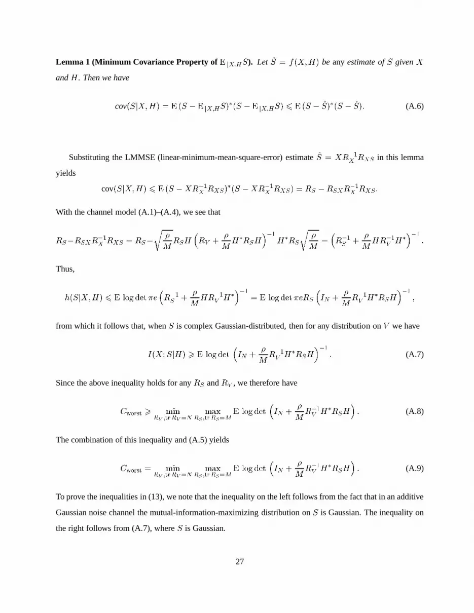
Lemma 1 (Minimum Covariance Property of E jX;HS). Let S = f(X;H) be anyestimate ofS givenXandH. Then we have

cov(SjX;H) = E (S � E jX;HS)�(S � E jX;HS) 6 E (S � S)�(S � S): (A.6)

Substituting the LMMSE (linear-minimum-mean-square-error) estimateS = XR�1X RXS in this lemma

yields

cov(SjX;H) 6 E (S �XR�1X RXS)�(S �XR�1X RXS) = RS �RSXR�1X RXS :With the channel model (A.1)–(A.4), we see thatRS�RSXR�1X RXS = RS�r �M RSH �RV + �MH�RSH��1H�RSr �M = �R�1S + �MHR�1V H���1 :Thus,h(SjX;H) 6 E log det�e�R�1S + �MHR�1V H���1 = E log det �eRS �IN + �MR�1V H�RSH��1 ;from which it follows that, whenS is complex Gaussian-distributed, then for any distribution onV we haveI(X;SjH) > E log det �IN + �MR�1V H�RSH��1 : (A.7)

Since the above inequality holds for anyRS andRV , we therefore haveCworst > minRV ;trRV =N maxRS ;trRS=M E log det �IN + �MR�1V H�RSH� : (A.8)

The combination of this inequality and (A.5) yieldsCworst = minRV ;trRV =N maxRS ;trRS=M E log det �IN + �MR�1V H�RSH� : (A.9)

To prove the inequalities in (13), we note that the inequality on the left follows from the fact that in an additive

Gaussian noise channel the mutual-information-maximizing distribution onS is Gaussian. The inequality on

the right follows from (A.7), whereS is Gaussian.

27

All that remains to be done is to compute the optimizingRV;opt andRS;opt, whenH is rotationally-

invariant. Consider firstRS;opt. There is no loss of generality in assuming thatRS is diagonal: if not, take

its eigenvalue decompositionRS = U�sU�, whereU is unitary and�s is diagonal, and note thatU�H has

the same distribution asH becauseH is left rotationally invariant. Now suppose thatRS;opt is diagonal with

possibly unequal entries. Then form a new covariance matrixRS = 1M !PM !m=1 PmRS;optP �m = IM , where

theP1; : : : ; PM ! are all possibleM �M permutation matrices. Since the “expected log-det” function in (A.9)

is concave inRS , the value of the function cannot decrease with the new covariance. We therefore conclude

thatRS;opt = IM . A similar argument holds forRV;opt because the “expected log-det” function in (A.9) is

convex inRV .

A.3 Correlated Noise

We can also find the worst case general additive noise, possibly correlated with the signalS. We do not use

this result in the body of the paper because it is not always amenable to closed-form analysis. For simplicity,

we assume a rotationally-invariant distribution forH.

Any arbitrary noise can be decomposed asV = V � SR�1S RSV| {z }V 0 +SR�1S RSV ; (A.10)

whereV 0is uncorrelated withS. Thus, (A.1) can be written asX = S�r �MH +R�1S RSV�+ V 0 :

DefiningA �= pMR�1S RSV , we have X = Sp�H +ApM + V 0 ; (A.11)

whereV 0 is uncorrelated withS and has the power constraint1N EV 0V 0� = 1N EV V � � 1MN ESAA�S� = 1� 1MN trA�RSA = �2V 0 :The worst-case uncorrelated noiseV 0 has therefore the distributionCN (0; �V 0IN ), and the capacity for the

28

channel (A.11) becomes E log det �IM + (p�H +A)(p�H +A)�M�2V 0 � :Since the capacity-achieving distribution onS is CN (0; IM ), 1 we haveRS = IM and so�2V 0 = 1 �1MN trA�A, so that the capacity becomesE log det IM + (p�H +A)(p�H +A)�M(1� 1MN trA�A) ! :Clearly, the worst-case additive noise is found by minimizing the above expression over the matrixA 2CM�N , subject to the constrainttrA�A 6MN . Hence, we have shown the following result.

Theorem 4 (Worst-Case Additive Noise).Consider the matrix-valued additive noise known channelX =r �M SH + V;whereH 2 CM�N is the known channel with a rotationally-invariant distribution, and where the signalS 2 C1�M and the additive noiseV 2 C1�N satisfy the power constraintsE 1MSS� = 1 and E 1N V V � = 1:Then the worst-case noise is given byV =q 1M SA+W , whereW is independent zero-mean Gaussian noise

with variance�2 = 1� 1N trAA�, i.e.,W � CN (0;q1� 1N trAA�IN ), and whereA 2 CM�N is the matrix

solution to Cworst = minfA;trAA�<MNgE log det IM + (p�H +A)(p�H +A)�M(1� 1MN trAA�) ! : (A.12)

We also have the minimax propertyIV�AS+CN (0;�2IN );S(X;S) 6 IV�AS+CN (0;�2IN );S�CN (0;IM )(X;S) = Cworst 6 IV;S�CN(0;IM )(X;S):(A.13)

We do not know how to find an explicit solution to the optimization problem (A.12) in general. When the

1Recall that the transmitter has no knowledge of the channelH, and hence of the matrixA, so that it cannot minimize the noisepower�2V 0 = 1� 1MN trA�RSA by a clever choice ofRS—the best it can do isRS = IM .

29

channel is scalar, however, we can solve it easily.

Corollary 3 (Scalar Case). Consider the scalar channel additive noise channelx = p�s+ v;where the signals and the additive noisev satisfy the power constraintsE jsj2 = E jvj2 = 1. Then the

worst-case noise is given byv = as + w wherew is independent zero-mean Gaussian noise with variance1� jaj2 and where a = 8<: �p� if � < 1�q1� if � > 1;The resulting worst-case capacity is C = 8<: 0 if � < 1log � if � > 1;

Note that, when� < 1, the noise has enough power to subtract out the effect of the signal so that the

resulting capacity is zero. When� > 1, however, the noise only subtracts out a “portion” of the signal and

reserves the remainder of its power for independent Gaussian noise. The resulting worst-case capacity islog �,

as compared withlog(1 + �), the worst-case capacity with uncorrelated noise. Thus, athigh SNR, correlated

noise does not affect the capacity much more than uncorrelated noise.

30

References

[1] I. E. Telatar, “Capacity of multi-antenna Gaussian channels,”Eur. Trans. Telecom., vol. 10, pp. 585–595,

Nov. 1999.

[2] G. J. Foschini, “Layered space-time architecture for wireless communication in a fading environment

when using multi-element antennas,”Bell Labs. Tech. J., vol. 1, no. 2, pp. 41–59, 1996.

[3] T. L. Marzetta, “BLAST training: Estimating channel characteristics for high-capacity space-time wire-

less,” in Proc. 37th Annual Allerton Conference on Communications, Control, and Computing, Sept.

22–24 1999.

[4] W. C. Jakes,Microwave Mobile Communications. Piscataway, NJ: IEEE Press, 1993.

[5] M. Medard, “The effect upon channel capacity in wirelesscommunication of perfect and imperfect

knowledge of the channel,”to appear in IEEE Trans. Info. Theory.

[6] B. Hochwald and W. Sweldens, “Differential unitary space time modulation,” tech. rep., Bell Labo-

ratories, Lucent Technologies, Mar. 1999. To appear inIEEE Trans. Comm.. Download available at

http://mars.bell-labs.com.

[7] B. Hughes, “Differential space-time modulation,”submitted to IEEE Trans. Info. Theory, 1999.

[8] V. Tarokh and H. Jafarkhani, “A differential detection scheme for transmit diversity,”to appear in J. Sel.

Area Comm., 2000.

[9] E. Biglieri, J. Proakis, and S. Shamai, “Fading channels: information-theoretic and communications

aspects,”IEEE Trans. Info. Theory, pp. 2619–2692, Oct. 1999.

[10] I. C. Abou-Faycal, M. D. Trott, and S. Shamai, “The capacity of discrete-time Rayleigh fading channels,”

in IEEE Int. Symp. Info. Theory, p. 473, June 1997. Also submitted toIEEE Trans. Info. Theory.

[11] L. Zheng and D. Tse, “Packing spheres in the Grassman manifold: a geometric approach to the nonco-

herent multi-antenna channel,”submitted to IEEE Trans. Info. Theory, 2000.

[12] T. Soderstrom and P. Stoica,System Identification. London: Prentice Hall, 1989.

31