arX

iv:a

stro

-ph/

0407

359v

1 1

6 Ju

l 200

4

Mon. Not. R. Astron. Soc. 000, 000–000 (0000) Printed 2 February 2008 (MN LATEX style file v2.2)

Host Galaxies of Gamma-Ray Bursts and their

Cosmological Evolution

Stephanie Courty, Gunnlaugur Bjornsson, Einar H. GudmundssonScience Institute, University of Iceland, Dunhaga 3, IS–107 Reykjavik, Iceland

e-mail: courty, gulli, einar@raunvis.hi.is

2 February 2008

ABSTRACT

We use numerical simulations of large scale structure formation to explore the cos-mological properties of Gamma-Ray Burst (GRB) host galaxies. Among the differentsub-populations found in the simulations, we identify the host galaxies as the mostefficient star-forming objects, i.e. galaxies with high specific star formation rates. Wefind that the host candidates are low-mass, young galaxies with low to moderate starformation rate. These properties are consistent with those observed in GRB hosts,most of which are sub-luminous, blue galaxies. Assuming that host candidates aregalaxies with high star formation rates would have given conclusions inconsistent withthe observations. The specific star formation rate, given a galaxy mass, is shown toincrease as the redshift increases. The low mass of the putative hosts makes themdifficult to detect with present day telescopes and the probability density function ofthe specific star formation rate is predicted to change depending on whether or notthese galaxies are observed.

Key words: cosmology: large-scale structure of the Universe – galaxies: formation –galaxies: evolution – gamma rays: bursts

1 INTRODUCTION

For three decades Gamma-Ray Bursts (GRBs) remained anenigma. The detection of optical afterglows associated witha GRB (see van Paradijs et al. 2000, for a review), revolu-tionized our understanding of the phenomena. A GRB isnow thought to occur when the core of a massive star col-lapses to form a black hole (Woosley 1993; Paczynski 1998;MacFadyen & Woosley 1999) (see also Meszaros 2002, fora review). In most cases when an optical afterglow from aGRB has been detected, they have been shown to occurin galaxies at intermediate or high redshifts. To date, theredshift of over 40 GRB afterglows and their host galax-ies have been measured. Because of the short lifetime ofa massive star, a GRB is generated essentially instanta-neously after the star’s formation, as compared to the evo-lutionary timescale of a typical galaxy or the cosmologicaltimescale. The bursts are therefore generally considered tobe good tracers of the history of massive star formation (e.g.Blain & Natarajan 2000).

It was early realized that because of their extremebrightness, GRBs and their afterglows might be detectableto very high redshifts and therefore might be useful ascosmological probes, in particular if the bursts possesseda ’standard candle’ like property (e.g. Lamb & Reichart2000). The main interest in the cosmological application

of GRBs has resulted from the increased understandingof the relation between GRBs and powerful supernovae(e.g. Hjorth et al. 2003; Stanek et al. 2003) and from therethe mapping of the cosmic star formation history (e.g.Ramirez-Ruiz et al. 2002, and references therein). Otherpossible applications have also been considered, such as theuse of bursts as probes of the interstellar medium in evolv-ing galaxies and as probes of primordial star formation andreionization, although these are observationally very chal-lenging at present (e.g. Djorgovski et al. 2003). Constructinga reliable Hubble diagram with GRB afterglows, however, islikely to remain a very difficult subject (Bloom et al. 2003).

In this paper, we take a different approach altogether.Instead of focusing on the diverse properties of the burststhemselves we use the fact that in almost all cases wheresufficiently deep observations have been carried out, a hostgalaxy has been discovered. Many of the host galaxies arevery faint, with R band magnitudes down to about 30(Jaunsen et al. 2003), and might have gone undetected hadnot a GRB occurred in them. We will occasionally referto the hosts as GRB selected galaxies. Unfortunately, thenumber of hosts is still too limited for statistical stud-ies, but this is likely to change after Swift is launchedin 2004. A number of first results on the hosts does ex-ist however, and a picture of their properties is beginningto emerge. The host morphology shows most of them to

2 Courty, Bjornsson & Gudmundsso

be dwarf galaxies, either compact, irregular or interacting,possibly merging, and they also tend to be blue in color(e.g. Bloom et al. 1998; Le Floc’h et al. 2003; Berger et al.2003). Many hosts are sub-luminous, with L/L∗ < 1, (e.g.Le Floc’h et al. 2003), with GRB 990705 a notable excep-tion (Le Floc’h et al. 2002). The star formation rate (SFR)in most hosts as inferred from optical observations show lowto intermediate activity, with SFR = 1 − 50M⊙/yr (e.g.Bloom et al. , 1999; Castro-Tirado et al. 2001; Fynbo et al.2001; Chary et al. 2002; Price et al. 2002). In a number ofcases the sub-mm and radio observations indicate a SFRthat is up to a factor of 10 higher than the optically inferredrates (Berger et al. 2003). Finally, Sokolov et al. (2001) andChary et al. (2002) infer a host galaxy mass, M , typically inthe range 2·108

−4·1010M⊙. In addition, the variation in thespecific star formation rate, SFR/M , from host to host ismodest, normally within a factor of a few (Chary et al. 2002;Christensen et al. 2004). In fact, Christensen et al. (2004)has shown that all the hosts in their sample have spectralenergy distributions similar to young starburst galaxies withsmall to moderate extinction. Comparing their sample withthe Hubble Deep Field, they find the hosts to be similarto the bluest of the field galaxies which have the highestspecific SFR.

As the bursts occur in galaxies, they can be viewed notonly as tracers of massive star formation, but also as tracersof galaxy formation and evolution. The study of GRBs andtheir host galaxies is therefore intimately linked to the studyof galaxy evolution in general. Although the presently knownhost sample indicates that bursts can occur in any type ofgalaxy, the majority of them are faint and show a dwarf-likemorphology. They may therefore belong to the faint endof the galaxy luminosity function. GRB selected galaxiesmay prove to be an important sub-population of the galaxypopulation and their study may thus provide informationabout the galaxy luminosity function not easily accessibleotherwise.

The aim of this paper is to investigate theoretically theproperties of the host galaxies of GRBs as well as their cos-mological evolution rather than to focus on the GRB pro-genitor and its properties. To this end, we use numerical sim-ulations of large scale structure formation with the aim ofidentifying objects in the simulations with properties corre-sponding to those observed in the hosts. The simulations weuse, were previously considered by Alimi & Courty (2004)to explore a number of galaxy properties such as the cosmicstar formation rate density and the galaxy mass function.The simulations reveal a significant population of low-massgalaxies whose existence raises a number of questions ongalaxy evolution. In this paper we concentrate on the in-stantaneous and the specific star formation rates of the sim-ulated galaxies. We identify a sub-population of the galaxieswith high specific star formation rate as the likely candidatesfor GRB hosts. We find that the majority of this putativehost population has low-mass and low to modest SFR, al-though a number of high-mass objects also have similar spe-cific rates. We then explore the properties and cosmic evo-lution of the simulated host population and compare to thegalaxy population as a whole.

In section 2, we describe the details of the numericalsimulations relevant for this study. In section 3 we introducethe instantaneous star formation rate and in particular the

specific star formation rate as a measure of the efficiency ofstar formation. We also discuss the properties of the generalgalaxy population at low redshift. In section 4 a similar dis-cussion is presented for high redshift and the cosmologicalevolution of the galaxy properties is explored. In section 5we propose interpretations of the observations and we arguethat GRB host galaxies may be a powerful tracer of the faintgalaxy population. Section 6 concludes the paper.

2 NUMERICAL SIMULATIONS

The simulations were performed with a 3D N-body/hydro-dynamical code, coupling a PM scheme for computing grav-itational forces with an Eulerian approach for solving thehydrodynamical equations. Shock heating is treated withthe artificial viscosity method (Von Neumann & Richtmyer1950). The radiative cooling processes included are: col-lisional excitation, collisional ionization, recombination,bremsstrahlung and Compton scattering. Collisional ion-ization equilibrium is not assumed and the cooling ratesare computed from the evolution of a primordial compo-sition hydrogen-helium plasma. The simulations also in-clude a model for galaxy formation, summarized below.The numerical procedures are described in more detail inCourty & Alimi (2004) and Alimi & Courty (2004). Thegalaxy properties discussed in the latter paper were foundto be consistent with observational data. This suggests thatthe galaxy formation model used here to investigate the na-ture of host galaxies of GRBs, captures the essence of thegalaxy formation process.

Numerical simulations of large scale structure formationdo not currently allow following the formation of objects ofmass lower than the scale of a grid cell, a few times 106 M⊙.But computing the thermodynamic properties of the gas andits cosmological evolution allow us to consider the physicalconditions needed to form a galaxy. The most importantcondition is that the gas cloud is collapsing, in the sensethat the cooling time is less than the dynamical time orthe free fall time (Rees & Ostriker 1977). We then identify,at each time step, gas regions satisfying this condition. Afraction of the gas mass is turned into an object, labeled a“stellar particle”, with a rate:

dmB

dt= −

mB

t∗, (1)

with mB(t) the available baryonic mass enclosed within thegas region at cosmic time t, and t∗ a characteristic timescale.The cosmological evolution of these particles is followed ina non-collisional way. To express the condition tcool < tff ,we define the cooling timescale tcool, computed from the in-ternal energy variation of the gas, and the dynamical timeor free fall time, tff =

√

3π/32Gρ. To make sure that gasregions giving birth to galaxies are correctly identified weuse additional criteria: the size of the gas cloud must be lessthan the Jean’s length given by λJ = cs(π/Gρ)1/2; the gasmust be in a converging flow: ∇·~v < 0; the baryonic densitycontrast, δB ≡ (δρ/ρ)B, must be higher than a threshold(1 + δB)s, here taken to be the value of the baryonic den-sity contrast at the turnaround, i.e. 5.5 as computed in thetop-hat collapse spherical model (Padmanabhan 1993). Thetotal matter density, including dark matter, baryonic mat-

GRB Host Galaxies 3

ter and stellar particles, is used in the expressions for thedynamical time and the Jean’s length. In each cell, checkingthat the four criteria described above are satisfied, a frac-tion ∆t/t∗ of the gas is turned into a stellar particle, with∆t the timestep of the simulation. If a stellar particle startsforming at cosmic time t0 when the baryonic mass enclosedwithin the grid cell is mB(t0), we assume that the particleis fully formed at time ti = t0 + ∆t. Using eq. (1), we findthat the final mass of the particle is given by

mi = mB(t0) − mB(ti) ≃ mB(t0)∆t

t∗. (2)

The characteristic time is taken to be t∗ = max(tff , 108 yr).The stellar particles are involved in the computation of thegravitational potential and their evolution is treated in thesame way as the collisionless dark matter.

Galaxy-like objects are then defined, at any redshift,by grouping the stellar particles with a friend-of-friend algo-rithm. This algorithm joins together all particles closer thana distance proportional to a link parameter η, usually takento be 0.2 (equivalent to selecting an overdensity of 187 inthe spherical collapse model). The mass range of the stellarparticles spans from 106 to 108 M⊙, but in what followswe only consider, at any redshift, galaxies with a total masshigher than 5 · 108M⊙, although a number of lower massgalaxies also form in the simulations. At z = 0, this lowergalaxy mass limit corresponds to a minimum of 11 stellarparticles per galaxy and at z = 3 it corresponds to a min-imum of 27 particles. The total number of galaxy objectsin the catalogs at z = 0, 1 and 3 are 1650, 2164 and 1602,respectively.

Through the formation of the stellar particles and theirgroupings we therefore have access to the formation historyof each galaxy at any redshift. The mass of the galaxy at anytime is the sum of the mass of its individual stellar particlesat that time. This mass is likely to be an estimate of all thestellar populations formed over the lifetime of the galaxy,as the dark matter component is not included in the galaxymass. We estimate the epoch of formation for a given galaxyas the mean epoch of formation of all stellar particles thegalaxy is composed of, weighted by the mass of each particle,i.e. tm1 =

∑

(miti)/∑

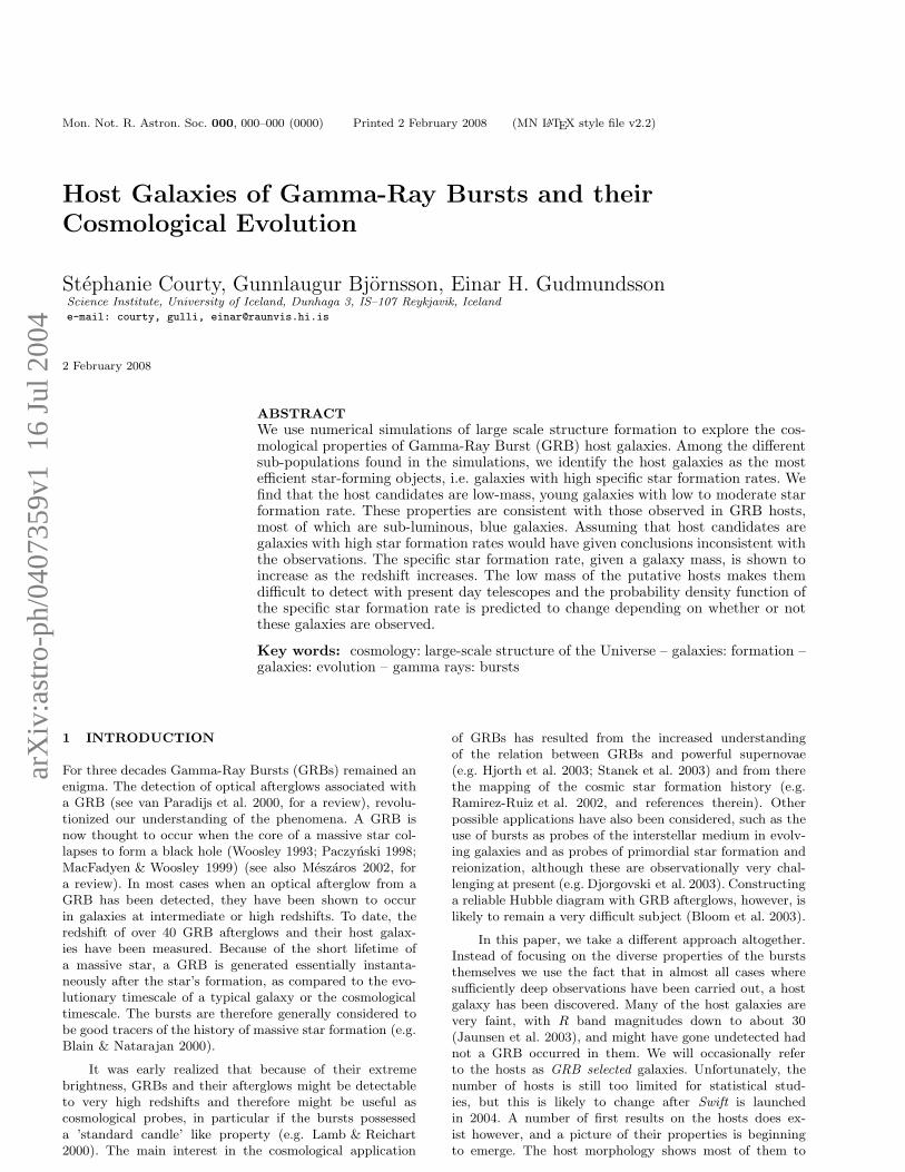
mi, where ti is the cosmic time cor-responding to the epoch of formation of stellar particle i. Analternative method would be to define the formation epochas the epoch, tm2, at which the galaxy has acquired half ofits final mass. Both methods give similar epoch estimates asshown in Figure 1. As the former method is based on theformation history of the stellar populations that make upthe galaxy, it resembles the way galaxy ages are estimatedobservationally, namely from the age of the stellar popula-tions in the galaxy. In this work, all formation epochs aretherefore estimated with the first method.

The results of this paper are given for a Λ−cold darkmatter model. The parameters of the simulations are: H0 =70 km s−1 Mpc−1, ΩK = 0, Ωm = 0.3, ΩΛ = 0.7,Ωb = 0.02h−2 with h = H0/100. The initial density fluc-tuation spectrum uses the transfer functions taken fromBardeen et al. (1986) with a shape parameter given bySugiyama (1995). The fluctuation spectrum is normalizedon COBE data (Bunn & White 1997) leading to a filtereddispersion at R = 8 h−1 Mpc of σ8 = 0.91. The resolutionof the simulations is as follows: the number of dark mat-

Figure 1. Comparing the two different ways of estimating theepoch of formation of galaxies, tm1 and tm2, computed from thegalaxy catalog at z = 0. See text for definitions.

ter particles is Np = 2563 and the number of grid cells isNg = 2563; the comoving size of the computational volumeis Lbox = 32 h−1Mpc, giving a dark matter particle massof 2.01 × 108 M⊙, and a gas mass initially enclosed in eachgrid cell of 3.09 × 107 M⊙.

3 INSTANTANEOUS STAR FORMATION

RATE AND EFFICIENCY OF STAR

FORMATION

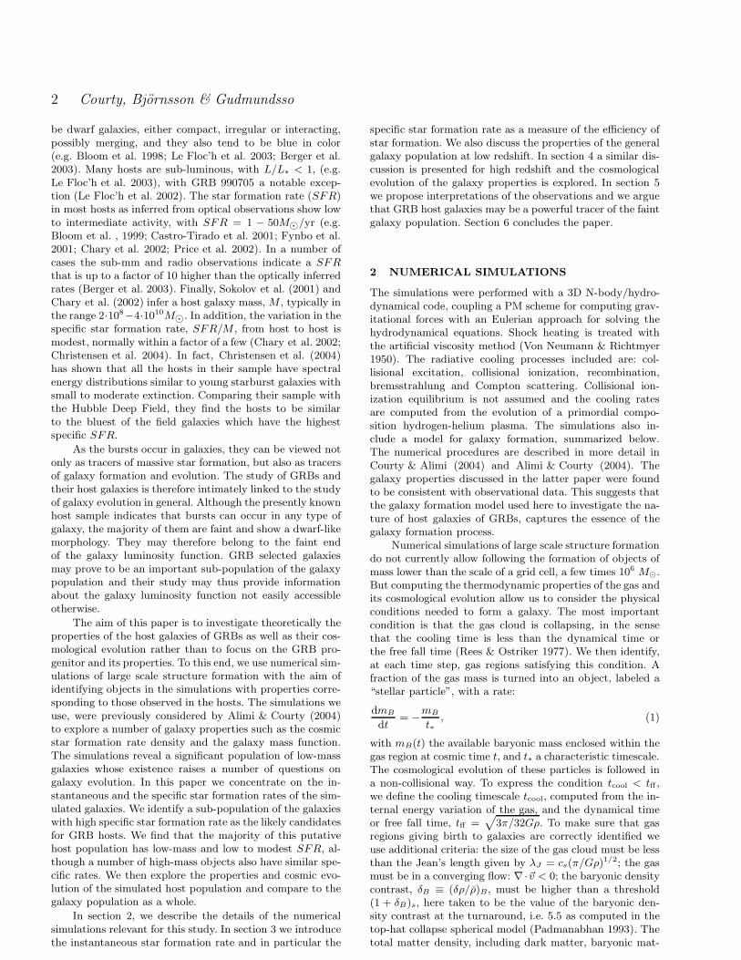
For each object at any given redshift z, corresponding tocosmic time tz, we compute the instantaneous star forma-tion rate SFR∗, where ∗ indicates a value obtained fromthe simulations. The instantaneous rate is computed fromthe mass in stellar populations in the galaxy that have ageless than τ at time tz, SFR∗ = ∆M/τ . This is equivalentto the baryonic mass ∆M , having been converted to starsduring time τ prior to the epoch under consideration. Notethat the SFR∗ depends both on τ and the cosmic time,SFR∗(τ, tz). It depends also on the amount of gas in thegalaxy that is available for star formation at tz since thestar formation rate in the model is proportional to the bary-onic density. We use τ = 0.1 Gyrs as representative valueat z = 0, time dilated at higher redshifts. Figure 2 showsa comparison between SFR∗ computed with τ = 0.05 andτ = 0.1 Gyrs for galaxies in the catalog at z = 3. Also indi-cated in the figure are the masses of the objects as explainedin the caption. We note that the star formation rates appearto be rather insensitive to the adopted value of τ , indicatingthat for most of the simulated galaxies, the SFR∗ is ratherconstant over a timescale of 0.1 Gyrs at high redshift (seealso Weinberg et al. (2002) for similar comparisons). Thereis some dispersion in the two estimates, mainly due to irreg-ularities in the star formation events in a given galaxy. Inaddition, some galaxies that have a non-zero SFR∗ as com-puted with τ = 0.1 Gyrs, show no star formation on shortertimescales. These galaxies are also shown in fig. 2, but as-signed an arbitrary value of SFR∗(τ = 0.05) = 0.03 M⊙/yr.For the low-mass objects with the lowest SFR∗, there is an

4 Courty, Bjornsson & Gudmundsso

Figure 2. Comparison between the instantaneous star formationrates, in units of M⊙/yr, computed for time dilated values ofτ = 0.1 Gyrs and τ = 0.05 Gyrs for the catalog at z = 3. Galaxieswith SFR∗ = 0.0 at τ = 0.05 Gyrs are plotted at SFR∗ = 0.03.Symbols denote the mass range of each galaxy: 5 ·108−5 ·109M⊙(crosses), 5 · 109 − 1011M⊙ (squares), M > 1011M⊙ (stars). Theinset shows a blow-up of the highest SFR∗-range.

apparent trend for the lower value of τ to yield a lower valueof SFR∗, up to a a factor of a few. The larger value of τsamples a longer period of star formation in the galaxy priorto the epoch under consideration and may therefore includeperiods of stronger star formation activity, resulting in ahigher SFR∗.

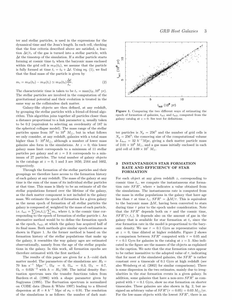
Figure 3 shows the SFR∗ as a function of the mass ofthe objects for the catalogs at z = 0 and z = 3. Galax-ies with non-zero SFR∗ are plotted arbitrarily at SFR∗ =0.01 M⊙/yr. In the former catalog, 572 objects have non-zero SFR∗ for τ = 0.1 Gyrs, while in the latter these objectsare 1470, but for clarity only 1000 randomly selected objectswith non-zero SFR∗ are plotted. Also indicated in fig. 3are three ranges of the epoch of formation of the galaxies.For the catalog at z = 0, the dividing epochs are z = 0.9,and z = 1.1, roughly corresponding to half and the third ofthe age of the Universe. For the catalog at z = 3, we usez = 3.9 and z = 4.3 as the dividing epochs. For both red-shifts, the instantaneous star formation rate increases lin-early with mass although there is considerable dispersionespecially at the lower redshift. For z = 0, this linearityholds only in the approximate mass range 1010

− 1011M⊙,for lower masses there is a large scatter in the SFR∗. Forthe higher redshift the linearity extends over two decades inmass. It is clear at both redshifts that the older objects tendto have lower SFR∗ than the younger objects and a slightlysteeper mass dependence than linear, though the differencedecreases with increasing redshift.

Note also, that galaxies of a given mass tend to have upto 10 times higher SFR∗ at z = 3 than at z = 0 and thatthe maximum SFR∗ in the catalogs decreases with redshiftfrom about 100 M⊙/yr at z = 3 to about 10-20 M⊙/yr atz = 0. It is interesting to note that these high SFR∗ val-ues at high redshift are consistent with the observationallyinferred SFR of Lyman-break galaxies at z = 3 (Giavalisco2002). The evolution of SFR∗ with redshift is very weakfor the low-mass objects in fig. 3, as their SFR∗ tends to

Figure 3. Instantaneous star formation rate as a function ofgalaxy mass, computed with τ = 0.1 Gyrs, for the catalogs atz = 3 (upper panel) and z = 0 (lower panel). For clarity, only1000 objects with non-zero SFR∗ are plotted from the catalogat z = 3. The symbols indicate the epoch of formation of eachgalaxy. In the upper panel they denote: epoch of formation lessthan z = 3.9 (dots), epochs in the range z = 3.9 − 4.3 (triangles)

and epochs greater than 4.3 (open circles). In the lower panel wehave: less than z = 0.9 (dots), in the range z = 0.9−1.1 (triangles)and greater than z = 1.1 (open circles). In both panels galaxieswith SFR∗ = 0.0 are plotted at SFR∗ = 0.01 M⊙/yr.

stay constant in time. The most dramatic difference in thecosmological evolution of the SFR∗ is seen in high-mass,old galaxies. The oldest (open circles) and most massive ob-jects have a SFR∗ up to two orders of magnitudes lowerthan their younger counterparts (dots). In fact, the star for-mation rate of massive, early-formed galaxies at z = 0 issimilar to that of the population of low-mass objects (fewtimes 109M⊙ or less), almost all of which are late-formedgalaxies.

Note that the plots in fig. 3 show a number of galax-ies which are not forming stars at the time of observation,tz. In these objects star formation has already ceased ormay be temporally stopped. These objects, although inac-tive, are quite numerous with most of them being of low-mass at both redshifts but being of higher mass as the red-shift decreases. At low redshift, most of the massive galaxiesshow no activity at all. These high-mass, inactive galaxiesreside in the center of the most massive dark matter halos(Alimi & Courty 2004) and, as the evolution progresses, the

GRB Host Galaxies 5

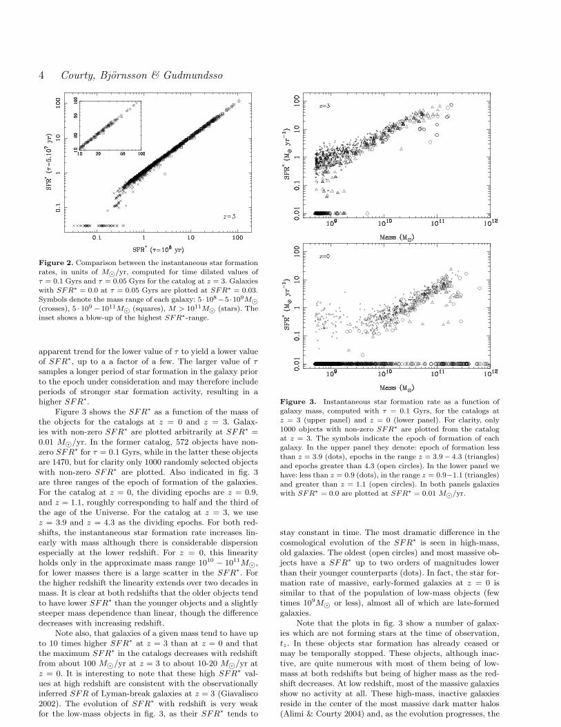
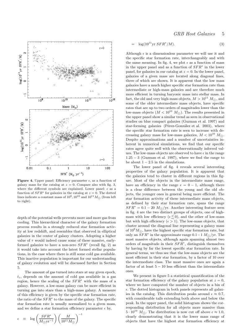
Figure 4. Upper panel: Efficiency parameter ǫ, as a function ofgalaxy mass for the catalog at z = 0. Compare also with fig. 3,where the different symbols are explained. Lower panel: ǫ as afunction of SFR∗ for galaxies in the catalog at z = 0. The dottedlines indicate a constant mass of 109, 1010 and 1011M⊙ (from leftto right).

depth of the potential wells prevents more and more gas fromcooling. This hierarchical character of the galaxy formationprocess results in a strongly reduced star formation activ-ity at low redshift, and resembles that observed in ellipticalgalaxies in the center of galaxy clusters. Adopting a highervalue of τ would indeed cause some of these massive, early-formed galaxies to have a non-zero SFR∗ (recall fig. 2) asit would take into account the latest formed stellar popula-tions, in the case where there is still some cold gas available.This inactive population is important for our understandingof galaxy evolution and will be discussed further in Section5.

The amount of gas turned into stars at any given epoch,tz, depends on the amount of cold gas available in a gasregion, hence the scaling of the SFR∗ with the mass of agalaxy. However, a low-mass galaxy can be more efficient inturning gas into stars than a high-mass galaxy. A measureof this efficiency is given by the specific star formation rate,the ratio of the SFR∗ to the mass of the galaxy. The specificstar formation rate is usually normalized to a given mass,and we define a star formation efficiency parameter ǫ by,

ǫ ≡ log

(

SFR∗

M⊙yr−1

)(

M

1011M⊙

)−1

= log(1011yr SFR∗/M). (3)

Although ǫ is a dimensionless parameter we will use it andthe specific star formation rate, interchangeably and withthe same meaning. In fig. 4, we plot ǫ as a function of massin the upper panel and as a function of SFR∗ in the lowerpanel, for galaxies in our catalog at z = 0. In the lower panel,galaxies of a given mass are located along diagonal lines,three of which are shown. It is apparent that the low massgalaxies have a much higher specific star formation rate thanintermediate or high-mass galaxies and are therefore muchmore efficient in turning baryonic mass into stellar mass. Infact, the old and very high-mass objects, M > 1011 M⊙, andsome of the older intermediate mass objects, have specificrates that are up to two orders of magnitudes lower than thelow-mass objects (M < 1010 M⊙). The results presented inthe upper panel show a similar trend as seen in observationalstudies on blue compact galaxies (Guzman et al. 1997) andstar-forming galaxies (Perez-Gonzalez et al. 2003), wherethe specific star formation rate is seen to increase with de-creasing galaxy mass for low-mass galaxies, M < 1010 M⊙.Despite approximations and a number of uncertainties in-herent in numerical simulations, we find that our specificrates agree quite well with the observationally inferred val-ues. The low-mass objects are observed to have ǫ in the range1.25 − 3 (Guzman et al. 1997), where we find the range tobe about 1 − 2.5 in the simulations.

The lower panel of fig. 4 reveals several interestingproperties of the galaxy population. It is apparent thatthe galaxies tend to cluster in different regions in this fig-ure. Most of the objects in the intermediate mass range,have an efficiency in the range ǫ = 0 − 1, although thereis a clear difference between the young and the old ob-jects, the younger ones in general being more efficient. Thestar formation activity of these intermediate mass objects,as defined by their star formation rate, spans the rangeSFR∗ = 0.1 − 20 M⊙/yr. Another interesting feature seenin fig. 4 are the two distinct groups of objects, one of high-mass with low efficiency (ǫ <

∼0), and the other of low-mass

but with high efficiency (ǫ > 1). The low-mass objects, thatcluster around the diagonal line representing a galaxy massof 109M⊙, have the highest specific star formation rate, butonly an SFR∗ in the approximate range 0.1−1 M⊙/yr. Themost massive objects, although again spanning almost twoorders of magnitude in their SFR∗, distinguish themselvesby having by far the lowest specific star formation rate. Ingeneral terms, we thus see that the low-mass objects are themost efficient in their star formation, by a factor of 10 overthe intermediate class. The most massive ones are again afactor of at least 5 − 10 less efficient than the intermediateones.

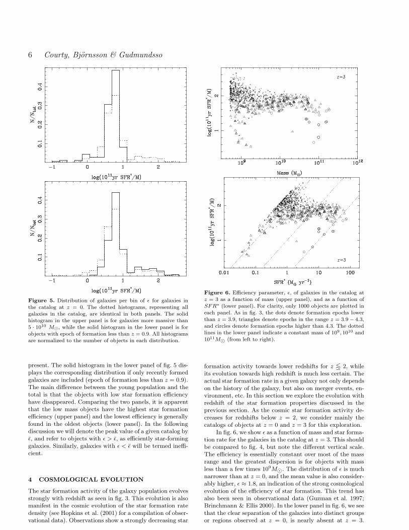
We present in figure 5 a statistical quantification of thestar formation efficiency of the galaxy population at z = 0,where we have computed the number of objects in a bin ofǫ. The dotted histogram in both panels represents all galax-ies in the catalog. This distribution peaks around ǫ ≈ 0.7,with considerable tails extending both above and below thepeak. In the upper panel, the solid histogram shows the cor-responding distribution for all objects more massive than5 · 1010 M⊙. The distribution is now cut off above ǫ ≈ 1.0,clearly demonstrating that it is the lower mass range ofobjects that have the highest star formation efficiency at

6 Courty, Bjornsson & Gudmundsso

Figure 5. Distribution of galaxies per bin of ǫ for galaxies inthe catalog at z = 0. The dotted histograms, representing allgalaxies in the catalog, are identical in both panels. The solidhistogram in the upper panel is for galaxies more massive than5 · 1010 M⊙, while the solid histogram in the lower panel is forobjects with epoch of formation less than z = 0.9. All histogramsare normalized to the number of objects in each distribution.

present. The solid histogram in the lower panel of fig. 5 dis-plays the corresponding distribution if only recently formedgalaxies are included (epoch of formation less than z = 0.9).The main difference between the young population and thetotal is that the objects with low star formation efficiencyhave disappeared. Comparing the two panels, it is apparentthat the low mass objects have the highest star formationefficiency (upper panel) and the lowest efficiency is generallyfound in the oldest objects (lower panel). In the followingdiscussion we will denote the peak value of a given catalog byǫ, and refer to objects with ǫ > ǫ, as efficiently star-forminggalaxies. Similarly, galaxies with ǫ < ǫ will be termed ineffi-cient.

4 COSMOLOGICAL EVOLUTION

The star formation activity of the galaxy population evolvesstrongly with redshift as seen in fig. 3. This evolution is alsomanifest in the cosmic evolution of the star formation ratedensity (see Hopkins et al. (2001) for a compilation of obser-vational data). Observations show a strongly decreasing star

Figure 6. Efficiency parameter, ǫ, of galaxies in the catalog atz = 3 as a function of mass (upper panel), and as a function ofSFR∗ (lower panel). For clarity, only 1000 objects are plotted ineach panel. As in fig. 3, the dots denote formation epochs lowerthan z = 3.9, triangles denote epochs in the range z = 3.9 − 4.3,and circles denote formation epochs higher than 4.3. The dottedlines in the lower panel indicate a constant mass of 109, 1010 and1011M⊙ (from left to right).

formation activity towards lower redshifts for z <≃ 2, while

its evolution towards high redshift is much less certain. Theactual star formation rate in a given galaxy not only dependson the history of the galaxy, but also on merger events, en-vironment, etc. In this section we explore the evolution withredshift of the star formation properties discussed in theprevious section. As the cosmic star formation activity de-creases for redshifts below z = 2, we consider mainly thecatalogs of objects at z = 0 and z = 3 for this exploration.

In fig. 6, we show ǫ as a function of mass and star forma-tion rate for the galaxies in the catalog at z = 3. This shouldbe compared to fig. 4, but note the different vertical scale.The efficiency is essentially constant over most of the massrange and the greatest dispersion is for objects with massless than a few times 109M⊙. The distribution of ǫ is muchnarrower than at z = 0, and the mean value is also consider-ably higher, ǫ ≈ 1.8, an indication of the strong cosmologicalevolution of the efficiency of star formation. This trend hasalso been seen in observational data (Guzman et al. 1997;Brinchmann & Ellis 2000). In the lower panel in fig. 6, we seethat the clear separation of the galaxies into distinct groupsor regions observed at z = 0, is nearly absent at z = 3.

GRB Host Galaxies 7

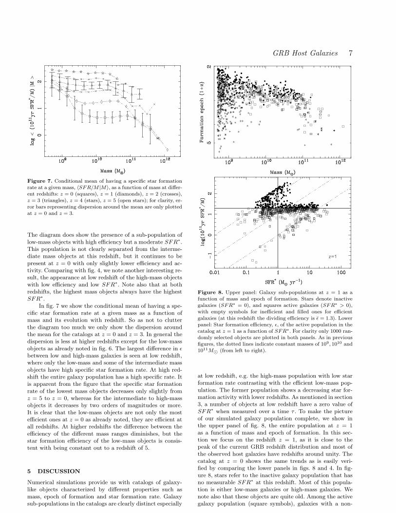
Figure 7. Conditional mean of having a specific star formationrate at a given mass, 〈SFR/M |M〉, as a function of mass at differ-ent redshifts: z = 0 (squares), z = 1 (diamonds), z = 2 (crosses),z = 3 (triangles), z = 4 (stars), z = 5 (open stars); for clarity, er-ror bars representing dispersion around the mean are only plottedat z = 0 and z = 3.

The diagram does show the presence of a sub-population oflow-mass objects with high efficiency but a moderate SFR∗.This population is not clearly separated from the interme-diate mass objects at this redshift, but it continues to bepresent at z = 0 with only slightly lower efficiency and ac-tivity. Comparing with fig. 4, we note another interesting re-sult, the appearance at low redshift of the high-mass objectswith low efficiency and low SFR∗. Note also that at bothredshifts, the highest mass objects always have the highestSFR∗.

In fig. 7 we show the conditional mean of having a spe-cific star formation rate at a given mass as a function ofmass and its evolution with redshift. So as not to clutterthe diagram too much we only show the dispersion aroundthe mean for the catalogs at z = 0 and z = 3. In general thedispersion is less at higher redshifts except for the low-massobjects as already noted in fig. 6. The largest difference in ǫbetween low and high-mass galaxies is seen at low redshift,where only the low-mass and some of the intermediate massobjects have high specific star formation rate. At high red-shift the entire galaxy population has a high specific rate. Itis apparent from the figure that the specific star formationrate of the lowest mass objects decreases only slightly fromz = 5 to z = 0, whereas for the intermediate to high-massobjects it decreases by two orders of magnitudes or more.It is clear that the low-mass objects are not only the mostefficient ones at z = 0 as already noted, they are efficient atall redshifts. At higher redshifts the difference between theefficiency of the different mass ranges diminishes, but thestar formation efficiency of the low-mass objects is consis-tent with being constant out to a redshift of 5.

5 DISCUSSION

Numerical simulations provide us with catalogs of galaxy-like objects characterized by different properties such asmass, epoch of formation and star formation rate. Galaxysub-populations in the catalogs are clearly distinct especially

Figure 8. Upper panel: Galaxy sub-populations at z = 1 as afunction of mass and epoch of formation. Stars denote inactivegalaxies (SFR∗ = 0), and squares active galaxies (SFR∗ > 0),with empty symbols for inefficient and filled ones for efficientgalaxies (at this redshift the dividing efficiency is ǫ = 1.3). Lowerpanel: Star formation efficiency, ǫ, of the active population in thecatalog at z = 1 as a function of SFR∗. For clarity only 1000 ran-domly selected objects are plotted in both panels. As in previousfigures, the dotted lines indicate constant masses of 109, 1010 and1011M⊙ (from left to right).

at low redshift, e.g. the high-mass population with low starformation rate contrasting with the efficient low-mass pop-ulation. The former population shows a decreasing star for-mation activity with lower redshifts. As mentioned in section3, a number of objects at low redshift have a zero value ofSFR∗ when measured over a time τ . To make the pictureof our simulated galaxy population complete, we show inthe upper panel of fig. 8, the entire population at z = 1as a function of mass and epoch of formation. In this sec-tion we focus on the redshift z = 1, as it is close to thepeak of the current GRB redshift distribution and most ofthe observed host galaxies have redshifts around unity. Thecatalog at z = 0 shows the same trends as is easily veri-fied by comparing the lower panels in figs. 8 and 4. In fig-ure 8, stars refer to the inactive galaxy population that hasno measurable SFR∗ at this redshift. Most of this popula-tion is either low-mass galaxies or high-mass galaxies. Wenote also that these objects are quite old. Among the activegalaxy population (square symbols), galaxies with a non-

8 Courty, Bjornsson & Gudmundsso

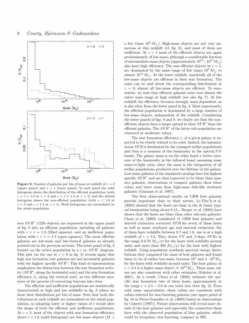
Figure 9. Number of galaxies per bin of mass at redshift of z = 3(upper panel) and z = 1 (lower panel). In each panel the solidhistogram shows the distribution of the efficient population (withǫ > ǫ = 1.8 at z = 3 and ǫ > ǫ = 1.3 at z = 1) and the dottedhistogram shows the non-efficient population (with ǫ < 1.8 atz = 3 and ǫ < 1.3 at z = 1). Both histograms are normalized onthe whole population.

zero SFR∗ (1239 objects) are separated in the upper panelof fig. 8 into an efficient population, including all galaxieswith ǫ > ǫ = 1.3 (filled squares), and an inefficient popu-lation with ǫ < ǫ = 1.3 (open squares). The most efficientgalaxies are low-mass and late-formed galaxies as alreadypointed out in the previous sections. The lower panel of fig. 8focuses on the active population in a ǫ vs. SFR∗ diagram.This plot (as the one at z = 0 in fig. 4) reveals again thathigh star formation rate galaxies are not necessarily galaxieswith the highest specific SFR∗. This kind of representationemphasizes the distinction between the star formation activ-ity (SFR∗, along the horizontal axis) and the star formationefficiency (ǫ, along the vertical axis), as two different mea-sures of the process of converting baryons into stars.

The efficient and inefficient populations are statisticallycharacterized at high and low redshifts in fig. 9 where weshow their distribution per bin of mass. Note that both dis-tributions at each redshift are normalized on the whole pop-ulation, so adopting lower or higher values of ǫ would alterthe shape of both the efficient and inefficient populations.At z = 3, most of the objects with star formation efficiencyabove ǫ = 1.8 (solid histogram) are low-mass objects (M <

a few times 109 M⊙). High-mass objects are not very nu-merous at this redshift (cf. fig. 6), and most of them areinefficient. At z = 1 most of the efficient objects are againpredominantly of low-mass, although a considerable fractionof intermediate mass objects (approximately 1010

−1011M⊙)also have high efficiency. The non-efficient objects at z = 1,are dominated by the mass range of few times 109 M⊙ toalmost 1012 M⊙. At the lower redshift, essentially all of thelow-mass objects are efficient in their star formation. Thesame can be said about the corresponding distribution atz = 0, almost all low-mass objects are efficient. To sum-marize, we note that efficient galaxies exist over almost theentire mass range at high redshift (see also fig. 7). At lowredshift the efficiency becomes strongly mass dependent, asis also clear from the lower panel in fig. 4. Most importantly,the efficient population is dominated by a large number oflow-mass objects, independent of the redshift. Consideringthe lower panels of figs. 6 and 8, we clearly see that the non-efficient objects have a larger spread in their SFR∗ than theefficient galaxies. The SFR∗ of the latter sub-population areclustered at moderate values.

The star formation efficiency, ǫ, of a given galaxy is ex-pected to be closely related to its color. Indeed, the instanta-neous SFR is dominated by the youngest stellar populationsand thus is a measure of the luminosity in the optical/UVbands. The galaxy mass is on the other hand a better mea-sure of the luminosity in the infrared band, assuming somemass-to-light ratio, since the mass is the integration of allstellar populations produced over the lifetime of the galaxy.Low-mass galaxies of the simulated catalogs have the highestspecific SFR∗ and are thus expected to be bluer than mas-sive galaxies; observations of compact galaxies show bluercolors and lower mass than high-mass disk-like starburstgalaxies (Guzman et al. 1997).

The first observational results on GRB host galaxiesprovide important clues to their nature. Le Floc’h et al.(2003) showed that the hosts are faint in the K band, typi-cal luminosities being about 0.1L∗. Berger et al. (2003) haveshown that the hosts are bluer than other sub-mm galaxies.Chary et al. (2002) considered 11 GRB host galaxies andderived extinction corrected SFR for seven of these hostsas well as mass, starburst age and internal extinction. Sixof them have redshifts between 0.7 and 1.6, one is at a highredshift of z = 3.4. They derive UV and β-slope SFRs inthe range 0.2-70 M⊙/yr for the hosts with redshifts aroundunity and more than 300 M⊙/yr for the host with highestredshift. Using population synthesis spectral energy distri-butions they computed the mass of host galaxies and foundthem to be of rather low-mass, between 108 and 4 · 109M⊙

for the hosts with redshifts around unity. The host galaxy atz = 3.4 is a higher mass object, 3 ·1010M⊙. These mass val-ues are also consistent with other estimates (Sokolov et al.2001). As a result, Chary et al. (2002) estimate the spe-cific star formation rate of these hosts, approximately inthe range ǫ = 2.5 − 3.9 in our units (see their fig. 2). Evenwith some uncertainties, these values are consistent withvalues inferred for star-bursting galaxies (see upper panel offig. 16 in Perez-Gonzalez et al. (2003) based on observationsby Calzetti (1997)). Future observations will reveal more de-tails of the host galaxies and especially the connection thesehave with the observed population of blue galaxies, whichcould be irregulars, star-bursting, compact or HII.

GRB Host Galaxies 9

Based on these host galaxy observations and on the factthat we can identify galaxy sub-populations in the simula-tions, we define our simulated candidate GRB host galaxiesas efficiently star-forming objects, with high specific starformation rate (filled squares in fig. 8) A galaxy is consid-ered a host if its efficiency is higher than ǫ, taken as the peakvalue of a given catalog. This value is rather arbitrary and islikely to be a lower limit, according to the observational esti-mate of the specific star formation rate in Christensen et al.(2004). The majority of these efficient galaxies in the sim-ulations are low-mass objects, but a modest peak in themass distribution around a few times 1010M⊙ is also seenin the lower panel of fig. 9. Such galaxies are expected to bearound 10 times less luminous than L∗ galaxies, consistentwith Le Floc’h et al. (2003). Moreover, the simulated hostgalaxy candidates are moderately active, with SFR∗ span-ning two orders of magnitude around unity. Their specificstar formation rates spans about one order of magnitude(fig. 8). Most of these galaxies are also low-mass objects,clustering around the line representing 109M⊙. This pic-ture seems consistent with observations: Although the hostgalaxies in Chary et al. (2002) show much higher specificstar formation rates than our candidates, it varies by a fac-tor of 20 and the host masses are generally around 109 M⊙.It is also interesting to note that one of their hosts withz = 3.4, has a similar ǫ as the hosts around z = 1, but witha much higher star formation rate and a galaxy mass thatis two orders of magnitude higher. The simulations show asimilar result, a 109 M⊙ galaxy has a specific star forma-tion rate in the range ǫ ≈ 1.3 − 2.6 at z = 1 (see fig. 8),which brackets the values obtained for a 1010 M⊙ galaxy atz = 3 (fig. 6). Recall also, that the SFR∗ increases at higherredshift for a given mass.

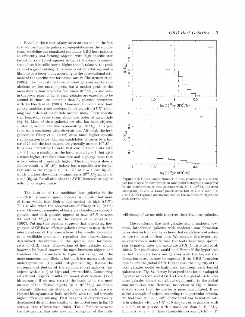
The location of the candidate host galaxies in theǫ − SFR∗ parameter space, appears to indicate that mostof them would have high ǫ and modest to high SFR∗.This is also what the observations of Chary et al. (2002)show. Moreover, a number of hosts are classified as compactgalaxies, and such galaxies appear to have SFR between0.1 and 14 M⊙/yr as in the sample of Guzman et al.(1997). Putting this together suggests that identifying hostgalaxies of GRBs as efficient galaxies provides us with firstinterpretations of the observations. Our results also pointto a verifiable prediction regarding the observationallydetermined distribution of the specific star formationrates of GRB hosts. Observations of host galaxies could,however, be biased towards the most luminous objects andtherefore the intermediate to high-mass range, with themore numerous and efficient, but much less massive, objectsunderrepresented. The solid histograms in fig. 10 show theefficiency distribution of the candidate host galaxies (i.e.objects with ǫ > ǫ) at high and low redshifts. Consideringall efficient objects results in broad distributions (solidhistograms). If we now restrict the hosts to be the mostmassive of the efficient objects (M > 1010M⊙), we obtainstrikingly different distributions. They are much narrower(dotted histograms) at both redshifts with the tail towardshigher efficiency missing. First versions of observationallydetermined distributions similar to the dotted ones in fig. 10already exist (Christensen 2002). The difference betweenthe histograms, illustrate how our perception of the hosts

Figure 10. Upper panel: Number of host galaxies (ǫ > ǫ = 1.8)per bin of specific star formation rate (solid histogram) comparedto the distribution of host galaxies with M > 1010M⊙ (dottedhistogram) at z = 3. Lower panel: same but at z = 1 with ǫ >ǫ = 1.3. Histograms are normalized to the number of objects ineach distribution.

will change if we are able to detect these low-mass galaxies.

The conclusion that host galaxies are, in majority, low-mass, late-formed galaxies with moderate star formationrates, derives from our hypothesis that candidate host galax-ies are the most efficient ones. We adopted this hypothesisas observations indicate that the hosts have high specificstar formation rates and moderate SFR (Christensen et al.2004). Our conclusions would be different if the hypothesisis that candidate hosts are galaxies with the highest starformation rates, as may be expected if the GRB formationrate follows the global SFR. In that case, the majority of thehost galaxies would be high-mass, inefficient, early-formedgalaxies (see Fig. 8). It may be argued that for our adoptedhypothesis to hold, and if GRBs trace the global SFR, low-mass galaxies should contribute significantly to the globalstar formation rate. However, inspection of Fig. 8, imme-diately shows that the matter is more complicated. If weselect a sample of objects according to a particular criteria,we find that at z = 1, 50% of the total star formation rateis in galaxies with a SFR∗ < 9 M⊙/yr; or in galaxies withǫ > 1.3; or in galaxies with a mass less than 5 · 1010M⊙.Similarly at z = 3, these thresholds become SFR∗ = 17

10 Courty, Bjornsson & Gudmundsso

M⊙/yr; or ǫ = 1.9; or M = 2 · 1010M⊙. Of course we haveto keep in mind that these numerical values depend on thephysics included in our simulations.

It is clear from Fig. 8 that if a higher specific star for-mation threshold is used to select candidate host galaxies,fewer hosts will have high SFR∗s. This would suggest thatthe GRB formation rate is not a tracer of the total starformation rate. The two rates follow each other (i) if thestellar mass function is independent of time and thus of thegalaxy properties (such as mass, age, metal content, etc),and (ii) if the probability that a high-mass star gives birthto a GRB event is independent of time. Although a numberof observational studies show that the stellar mass functiondepends on the galaxy type (Contini et al. 1995; Kroupa2001; Larson 2003), most workers assume a universal initialmass function independent of time. Moreover, the under-lying physics involved in the gamma-ray burst phenomenaimplies, among other things, that low-metalicity stars are fa-vored. Such low-metalicity environments should mainly existin young or starbursting or interacting galaxies rather thanin evolved systems even if these may be forming high-massstars. Similar caveats have been discussed in other contextsby Ramirez-Ruiz et al. (2002) and Choudhury & Srianand(2002). Observing host galaxies with properties such as ahigh specific star formation rate, could reinforce the factthat the probability of forming a GRB event from a high-mass star does depend on time and thus on the galaxy.

6 CONCLUSIONS

We have used numerical simulations of large scale structureformation to identify galaxy like objects and to follow theirevolution. We concentrated on the mass, the epoch of forma-tion and the instantaneous and specific star formation ratesof the objects. Our most important results are as follows:

The whole galaxy population includes a significant num-ber of low-mass objects with M < 1010M⊙. There is astrong cosmological evolution of the properties of the galaxypopulation between z = 3 and z = 0. We emphasize thatthe star formation rate of a galaxy should be considered ameasure of its star formation activity, while the specific starformation rate is a measure of its star formation efficiency.These properties are nicely illustrated in a diagram of ǫ vs.SFR∗ (fig. 8), where we find a number of clearly distinctsub-populations of galaxies.

The low-mass population is further divided into sub-populations, some of which have a high specific star forma-tion rate. Based on these findings and on the first observa-tional results of GRB hosts, we identify candidate hosts inthe simulations as galaxies with high specific SFR∗, ratherthan objects with high star formation rate. The majorityof these candidate host galaxies appear to be of low mass,with recent formation epochs and a moderate SFR∗ of a fewM⊙/year or lower. The properties of the candidate hosts soidentified, are consistent with the trends observed in theGRB host galaxies. An implication of our conclusions, giventhe applicability of the physical input in the simulations usedhere, is that GRBs may not trace the cosmic star formationrate.

Most of the observed GRB hosts to date have a redshiftaround unity. We show that the efficiency of the low-mass

galaxies does not vary much with redshift. For high redshift,more and more galaxies are found to be efficient independentof mass, while the efficiency of intermediate to high-massgalaxies decreases strongly with decreasing redshift.

As the low-mass objects are very faint, the observationsof GRB host galaxies will initially be observationally biasedtowards the intermediate and high-mass objects. These willbe easier to detect due to their higher luminosity. They willtypically have an SFR in the range 1 − 40M⊙/year at aredshift of unity. It may take the next generation spacetelescopes to reveal the properties of the low-mass sub-population of host galaxies. These are expected to outnum-ber the currently observable hosts by a considerable factor.

Furthermore, the low-mass galaxy population is knownto be important for the understanding of galaxy formation.GRB host galaxies may thus become useful tracers of thispopulation or in fact the faint end of the galaxy luminos-ity function that may be difficult to detect otherwise. ThusGRB selected host galaxies may become an important linkin the study of structure formation and evolution. AlthoughGRB selected galaxies introduce its own ’selection effect’,they are free from others affecting surveys of various kinds,such as the magnitude limited observations of optical sur-veys and the sensitivity limitation of the sub-mm observa-tions.

ACKNOWLEDGMENTS

We thank the anonymous referee for constructive commentsthat helped improve the paper. This work was supportedby a Special Grant from the Icelandic Research Council.The numerical simulations used in this paper were per-formed on NEC-SX5 at the Institut du Developpement etdes Ressources en Informatique Scientifique (France).

REFERENCES

Alimi J.-M., Courty S., 2004, A&A submittedBardeen J., Bond J., Kaiser N., Szalay A. S., 1986, ApJ,304, 15

Berger E., Cowie L. L., Kulkarni S. R., Frail D. A., AusselH., Barger A. J., 2003, ApJ, 588, 99

Blain A. W., Natarajan P., 2000, MNRAS, 312, L35Bloom J. S., Djorgovski S. G., Kulkarni S. R., Frail D. A.,1998, ApJ, 507, L25

Bloom J. S., Frail D. A., Kulkarni S. R., 2003, ApJ, 594,674

Bloom J. S. et al., 1999, ApJ, 518, L1Brinchmann J., Ellis R. S., 2000, ApJ, 536, L77Bunn E. F., White M., 1997, ApJ, 480, 6Calzetti D., 1997, AJ, 113, 162Castro-Tirado A. J. et al., 2001, A&A, 370, 398Chary R., Becklin E. E., Armus L., 2002, ApJ, 566, 229Christensen L., 2002, MS Thesis, University of CopenhagenChristensen L., Hjorth J., Gorosabel J., 2004, A&A, sub-mitted

Choudhury T. R., Srianand R., 2002, MNRAS, 336, L27Contini T., Davoust E., Considere S., 1995, A&A, 303, 440Courty S., Alimi J.-M., 2004, A&A 416, 875

GRB Host Galaxies 11

Djorgovski S. G. et al., 2003, in Discoveries and ResearchProspects from 6- to 10-Meter-Class Telescopes II. Editedby Guhathakurta, Puragra. Proceedings of the SPIE, Vol-ume 4834 The cosmic gamma-ray bursts and their hostgalaxies in a cosmological context. pp 238–247

Fynbo J. U. et al., 2001, A&A, 373, 796Giavalisco M., 2002, ARA&A, 40, 579Guzman R., Gallego J., Koo D. C., Phillips A. C., Lowen-thal J. D., Faber S. M., Illingworth G. D., Vogt N. P.,1997, ApJ, 489, 559

Hjorth J. et al., 2003, Nature, 423, 847Hopkins A. M., Connolly A. J., Haarsma D. B., Cram L. E.,2001, AJ, 122, 288

Jaunsen A. O., Andersen M. I., Hjorth J., Fynbo J. P. U.,Holland S. T., Thomsen B., Gorosabel J., Schaefer B. E.,Bjornsson G., Natarajan P., Tanvir N. R., 2003, A&A,402, 125

Kroupa P., 2001, MNRAS, 322, 231Lamb D. Q., Reichart D. E., 2000, ApJ, 536, 1Larson R. B., 2003, in ASP Conf. Ser. 287: Galactic StarFormation Across the Stellar Mass Spectrum The StellarInitial Mass Function and Beyond (Invited Review). pp65–80

Le Floc’h E., Duc P.-A., Mirabel I. F., Sanders D. B., BoschG., Diaz R. J., Donzelli C. J., Rodrigues I., CourvoisierT. J.-L., Greiner J., Mereghetti S., Melnick J., Maza J.,Minniti D., 2003, A&A, 400, 499

Le Floc’h E., Duc P.-A., Mirabel I. F., Sanders D. B., BoschG., Rodrigues I., Courvoisier T. J.-L., Mereghetti S., Mel-nick J., 2002, ApJ, 581, L81

Meszaros P., 2002, ARA&A, 40, 137MacFadyen A. I., Woosley S. E., 1999, ApJ, 524, 262Perez-Gonzalez P. G., Gil de Paz A., Zamorano J., Gal-lego J., Alonso-Herrero A., Aragon-Salamanca A., 2003,MNRAS, 338, 525

Paczynski B., 1998, ApJ, 494, L45Padmanabhan T., 1993, Structure formation in the Uni-verse. Cambridge University Press

Price P. A. et al., 2002, ApJ, 573, 85Ramirez-Ruiz E., Trentham N., Blain A. W., 2002, MN-RAS, 329, 465

Rees M. J., Ostriker J. P., 1977, MNRAS, 179, 541Sokolov V. V. et al., 2001, A&A, 372, 438Stanek, K. Z. et al., 2003, ApJ, 591, L17Sugiyama N., 1995, ApJS, 100, 281van Paradijs J., Kouveliotou C., Wijers R. A. M. J., 2000,ARA&A, 38, 379

Von Neumann J., Richtmyer R., 1950, J. Appl. Phys., 21,232

Weinberg D. H., Hernquist L., Katz N., 2002, ApJ, 571, 15Woosley S. E., 1993, ApJ, 405, 273