History, Path Dependence and Development: Evidencefrom Colonial Railroads, Settlers and Cities in Kenya∗

Remi Jedwab† and Edward Kerby‡ and Alexander Moradi§

This Version: January 2015

Abstract: Little is known about the extent and forces of urban path dependence in devel-

oping countries. Colonial era railroad construction in Kenya provides a series of natural

experiments to study the emergence and persistence of spatial equilibria. Using new data

at a fine spatial level spanning over one century shows that colonial railroads determined

the location of European settlers, which in turn determined the location of the main cities

and Asian traders at independence. Both Europeans and Asians were relatively skilled.

Europeans then left following the Lancaster House Agreement of 1962, many Asians de-

parted following the Trade Licensing Act of 1967, and railroads declined in the 1960s-

1970s, constituting three local negative shocks to physical and human capital. Yet the

colonial cities persisted. We test four different explanations for path dependence based on

institutional persistence, technological change, sunk investments, and spatial coordination

failures. We also discuss the role of human capital in urban growth and persistence.

Keywords: Path Dependence; Transport; Settler Colonialism; Human Capital; Cities

JEL classification: R11; R12; R40; O18; O33; I25; N97

∗We are grateful to David Albouy, Hoyt Bleakley, Dan Bogart, Maarten Bosker, Leah Brooks, Denis Cogneau,James Fenske, John Gallup, Edward Glaeser, Rafael Gonzalez-Val, Gordon Hanson, Vernon Henderson, RichardHornbeck, Stephen Smith, Adam Storeygard, Anthony Yezer, Leonard Wantchekon and seminar audiencesat the 3rd Workshop on Urban Economics (Barcelona), African Economic History Network Meeting (SimonFraser), ASSA meetings (Philadelphia), Cambridge (RES), Cape Town (UCT and Climate, Geography andEconomic History Conference), the Economic History Association Meeting (Washington), CSAE (Oxford),DIAL (Paris), EPEN (CIDE-Princeton), Erasmus University Rotterdam, George Mason-George Washington Eco-nomic History Workshop, George Washington, IEA (Jordan), London School of Economics, RES (Manchester),Maryland, Portland State, Stellenbosch, Stockholm, Sussex, UC-Irvine, Urban Economics Association Meeting(Washington), VU University Amsterdam, Wageningen and Wits for helpful comments. We are grateful toDominic Bao for excellent research assistance. This paper was previously circulated as “Out of Africa: ColonialRailroads, White Settlement and Path Dependence in Kenya”. We gratefully acknowledge the support of theInstitute for International Economic Policy and the Elliott School of International Affairs at GWU.

†Remi Jedwab, Department of Economics, George Washington University, 2115 G Street, NW, Washington,DC 20052, USA (e-mail: jedwab@gwu.edu).

‡Edward Kerby, Department of Economic History, London School of Economics and Political Science,Houghton Street, London WC2A 2AE, UK (email: e.m.kerby@lse.ac.uk).

§Corresponding Author: Alexander Moradi, Department of Economics, University of Sussex, Jubilee Build-ing, Falmer, BN1 9SN, UK (email: A.Moradi@sussex.ac.uk). Also affiliated with the Center for the Study ofAfrican Economies, University of Oxford, Department of Economics, Manor Road, Oxford, OX1 3UQ, UK, andResearch Associate, Department of Economics, Stellenbosch University, South Africa.

From Mombasa is the starting-point of one of the most wonderful railways in the world [...] a

sure, swift road along which the white man and all that he brings with him, for good or ill, may

penetrate into the heart of Africa as easily and safely as he may travel from London to Vienna.

Winston Churchill, My African Journey, 1908

1. INTRODUCTION

Cities are the main engines of growth (Lucas, 1988). By agglomerating people, cities

facilitate the exchange of goods and ideas, increasing aggregate productivity (Glaeser &

Gottlieb, 2009), and therefore can promote growth in developing countries (Henderson,

2010; Duranton, 2014). Studying why cities emerge and persist has become crucial to our

understanding of this growth process, and the evolution of spatial inequality both across

and within countries (Desmet & Henderson, 2014).

The development and urban literatures have argued over whether geography (i.e., natural

advantages) or history (i.e., man-made advantages) are the main determinants for the

spatial distribution of economic activity (i.e., cities). Studies have shown that geography has

a strong influence on spatial development, in both rich and poor countries (Gallup, Sachs

& Mellinger, 1999; Beeson, DeJong & Troesken, 2001; Rappaport & Sachs, 2003; Bosker &

Buringh, 2010; Maloney & Caicedo, 2012). One implication of geography as a driver for

development is that localised historical shocks should only have temporary effects. Davis &

Weinstein (2002, 2008), Bosker et al. (2007, 2008) and Miguel & Roland (2011) use the war

time bombing of Japan, Germany and Vietnam respectively, to test whether these shocks had

long-term effects on the relative ranking of cities that were disproportionately demolished.

Many of these destroyed cities recovered their population, which therefore showed that

serial correlation explained urban persistence. Davis & Weinstein (2002) concluded that

there is only one spatial equilibrium, which is determined by geography. If only geography

matters, regional policies could be ineffective in altering regional development.

Conversely, the literature has also established that localised historical shocks can have

permanent spatial effects. For example, Redding, Sturm & Wolf (2011) showed how

the division of Germany, despite later reunification, permanently changed the location

of its main airports. Likewise, Nunn & Puga (2012) demonstrated how the slave trade

permanently altered the location choice of Africans, although the trade ended one century1

ago. These studies, and others (Bosker et al., 2008; Bleakley & Lin, 2012; Ahlfeldt et al.,

2012; Michaels & Rauch, 2013; Jedwab & Moradi, 2014), show how there may be path

dependence in space. It suggests the existence of multiple spatial equilibria, with the

selection of one of these equilibria being determined by history. This historical importance

leaves a role for regional policies since they may alter regional development.

Local increasing returns have been advanced as the main explanation for path dependence.

Krugman (1991) contrasts the role of “history” and “expectations” in explaining increasing

returns. First, fixed costs can be a source of increasing returns where man-made advantages

(or history in the Krugmanian sense) may account for the path dependence. Examples are

ports (Fujita & Mori, 1996), or durable housing (Glaeser & Gyourko, 2005). Second, given

local increasing returns, factors must also be co-located in the same locations. Intervening

are spatial coordination failures, as it is not obvious which locations will have the factors.

Cities solve this problem by signalling to productive agents where they could expect others

to locate (Bleakley & Lin, 2012; Jedwab & Moradi, 2014). However, politics may also be a

factor of path dependence if governments purposely use public expenditure to preserve an

existing spatial distribution (Davis & Weinstein, 2002).

In this paper, we use a series of large exogenous shocks to investigate the extent and forces

of urban path dependence in a developing country. We focus on Kenya, for which we create

a new dataset on railroads, European and Asian settlements, and city growth at a fine spatial

level over one century (473 locations, approx. 16 x 16 km, from 1901 - 2009).

We first show how the construction of the colonial railroad created a new spatial equilibrium

in Kenya. For geo-strategic reasons, the British coloniser built a railroad from Mombasa, on

the coast, to Lake Victoria, in the hinterland. Although the line crossed Kenya from east to

west, the ultimate objective was to link the coast to Uganda (across Lake Victoria), where the

Nile originates; the control of which was regarded as a vital asset in the Scramble for Africa.

Our results show that the railroad had a strong impact on European settlement, establishing

cities from where the European settlers managed their commercial farms and specialised in

urban activities. Asian settlers then established themselves as traders in those cities. Both

groups were relatively skilled. Investments in public physical capital thus attracted human

capital during the colonial era. We then use various standard identifications strategies to

attempt to measure causal effects.

2

We test the persistence of this spatial equilibrium using three local negative shocks in

the immediate post-independence period. First, the European settlers left following the

Lancaster House Agreement of 1962. Europeans were required after independence to

choose their citizenship. Their refusal to give up the British citizenship resulted in an exodus

from Kenya. Second, many Asian settlers departed following the Trade Licensing Act of

1967, that discouraged them from owning or managing commercial establishments. Third,

the colonial railroad declined in the 1960s-1970s, mainly due to mismanagement and a lack

of maintenance in the sector, but also as extensive investments in sealed roads escalated,

especially in the locations farther away from the railroads. Thus, the three factors that gave

rise to the spatial equilibrium in the first place disappeared, and an entirely different spatial

distribution could have emerged in the post-independence period. However, we find that

locations that were disproportionately affected by these large shocks to physical capital and

human capital remain relatively more urban and developed today.

We use data on colonial and post-colonial infrastructure to investigate the channels of path

dependence. We contrast four different explanations based on institutional persistence,

technological change, sunk investments and spatial coordination failures. First, we argue

that institutional persistence, the fact that the new African political elite may have preserved

the colonial spatial equilibrium in order to better control the resources of the country, does

not account for path dependence. Second, we verify that path dependence is not explained

by changes in transport technology, as measured by roads (that replaced rail), and the

diffusion of knowledge, as measured by schools (that trained Africans who replaced the

settlers). Third, colonial cities were better endowed in infrastructure (e.g., hospitals) at

independence. We find that colonial sunk investments partially explains path dependence.

Fourth, we argue that persistence is also explained by the fact that the early emergence of

the railroad and settler cities served as a mechanism to coordinate spatial investments in

subsequent periods. In particular, we contend that expectations (i.e., spatial coordination

failures) may matter as much as history (i.e., sunk investments), which suggests that

regional policies may be ineffective if they do not also change expectations.

This study makes the following contributions to the literature. First, the natural experiment

allows us to examine the emergence and persistence of a spatial equilibrium. Studying

an initially unurbanised country allows us to analyse the emergence of the equilibrium,

whereas many studies have only tested if an equilibrium persists in the face of a shock.3

Kenya provides this ideal case, as it had only four coastal cities before colonisation. We then

use multiple shocks, the construction and demise of railroads, and the respective settlements

and exoduses of Europeans and Asians, to test for the persistence of the equilibrium. If

geography is time-invariant, having several symmetrical shocks helps identify the role of

increasing returns (Ahlfeldt et al., 2012). Second, we exploit shocks to physical capital

(railroads) and human capital (skilled settlers), and their interactions, to test their role in

path dependence. Jedwab & Moradi (2014) focus on rail building in Ghana. Kenya, unlike

Ghana, was a settler colony and saw a significant influx of European and Asian settlers

along the railroads. We find similar results no matter the shock studied. Third, we study

the mechanisms of urban path dependence, which few papers have done with the exceptions

of Bleakley & Lin (2012), Michaels & Rauch (2013) and Jedwab & Moradi (2014). Lastly,

we focus on a developing country, for which the extent and forces of path dependence could

differ. Geography could play a larger role in agrarian countries. Yet, any localised historical

shock could have substantial effects in rural countries. These effects will be permanent if

there are increasing returns. We find that both sunk investments and the solving of spatial

coordination failure therefore matters. Institutional persistence is then a well-documented

mechanism of path dependence across countries (Acemoglu, Johnson & Robinson, 2001).

However, it does not appear to be a significant channel within Kenya.

Our focus on transportation is associated with the recent literature on railroads and

economic growth (Atack et al., 2010; Banerjee, Duflo & Qian, 2012; Baum-Snow et al.,

2012, 2014; Donaldson, 2013; Donaldson & Hornbeck, 2013). For Africa, Jedwab & Moradi

(2014) find that railroads, a typical investment in physical capital during the colonial era,

had a strong impact on long-term development. In addition, the Kenyan context allows us

to study the relationship between human capital and city growth (see Henderson (2007)

and Glaeser & Gottlieb (2009) for two recent surveys). The literature has shown how cities

helped disseminate knowledge, which then promoted their growth (Glaeser, Scheinkman

& Shleifer, 1995; Simon, 1998; Glaeser & Saiz, 2004; Moretti, 2004; de la Roca & Puga,

2012; Gennaioli et al., 2013). The literature on human capital spillovers in developing

countries is scarcer (Henderson, 2010). The departure of settlers may have had asymmetric

spatial effects in Kenya. Yet, the cities with more settlers at independence, and thus a

larger exodus post-independence, were not durably affected by the shock. This suggests

that human capital may not be critical for city growth in our context, but rather cities solve4

a spatial coordination problem for skilled workers. In other words, skilled workers sort

themselves in the cities, which is consistent with the literature on spatial sorting (Combes,

Duranton & Gobillon, 2008; Young, 2013; Behrens, Duranton & Robert-Nicoud, 2014). The

result that human capital may have not mattered locally in 20th century Kenya is in line

with Michaels, Rauch & Redding (2013) and Glaeser, Ponzetto & Tobio (2014) who find

that human capital externalities were lower in the U.S. in the 19th century than in the 20th

century. Our interpretation of this result is that human capital externalities may matter more

for a skill-intensive economy, which Kenya was not during our period of study.

Lastly, the paper contributes to the literature on the economic effects of expulsions.

Waldinger (2010), Acemoglu, Hassan & Robinson (2011), Yuksel & Yuksel (2014) and

Pascali (2014) find negative local effects of the expulsions or elimination of Jews in various

contexts. These negative spillovers are explained by the fact that the Jews were skilled and

part of the middle class. Chaney & Hornbeck (2014) then find that the expulsions of Morisco

farmers in 17th century Spain had positive effects on the income per capita of non-Moriscos,

as the expulsions of the former freed land for the latter. Our context is different in that the

Europeans and the Asians were the economic elite of Kenya’s colonial cities. The fact that

we find no negative effects for the exodus of either group is consistent with the Malthusian

hypothesis that a population decline may cause temporary increases in income per capita,

which in turn leads to population convergence (the negative short-run effects disappear in

the long-run). It also shows that the human capital of the settlers was not essential to the

local Kenya economy (although their expulsion may have had aggregate effects).

The article proceeds as follows. Section 2 and 3 discusses the historical background

and presents the assembled data. Section 4 shows the emergence of the colonial spatial

equilibrium. Section 5 studies the persistence of this spatial equilibrium. Section 6 discusses

the results.2. HISTORICAL BACKGROUND

This section discusses the construction and demise of the colonial railroad, the mass inward

migration and subsequent exodus of Europeans and Asians. The following summary draws

from Hill (1950), Morgan (1963), Soja (1968), Sorrenson (1968) and Kapila (2009).

2.1 Construction and Demise of the Colonial Railroad

Kenya was extremely poor in the late 19th century. With the exception of Nairobi, founded

in 1899, there were only four towns in 1901, all of which were on the coastline. The5

various tribes were geographically separated by the Rift Valley, which served as a buffer

zone between them (see “Kikuyu”, “Kalenjin”, “Luhya”, “Luo” and “Maasai” in Figure 1).

Economic activity was constrained by high trade costs. Kenya lacked navigable waterways.

Draft animals had not been adopted due to the Tsetse fly. Head-loading was the main means

of transport, and very costly. Figures in Hill (1950) indicate a 1902 freight rate of 11 shillings

(s) per ton mile for head porterage as compared to 0.09s per ton mile by rail.1

The Uganda Railway was constructed between 1896-1901, mostly for geopolitical reasons.

The British thought that by linking Uganda to the coast they could unify all their colonies in

Northern, Eastern and Southern Africa.2 The British perceived Lake Victoria, the source of

the Nile River, to be vital for their interests in Egypt. The railroad shielded the region against

competing European powers, allowing the fast transport of troops. Secondly, Uganda was

seen to hold vast wealth with further trade potential. Linking Lake Victoria to the coast

would open up Uganda to trade. Kenya was merely a transit territory en route to Uganda.

The construction was debated fiercely within the British parliament. Critics doubted the

usefulness of the railroad “from nowhere to utterly nowhere”.

Railroad placement was driven by one objective, as evidenced in parliamentary records

and railroad surveys at that time: connecting Kisumu (on Lake Victoria) to Mombasa via

Nairobi at the least possible cost. Nairobi was chosen as the intermediary node because

it supplied rail construction workers and steam locomotives with water. At the time an

uninhabited swamp, Nairobi became the railroads headquarters in 1899 and the capital

soon thereafter. Railroad placement between the nodes was determined by topography.

Based on topography, the least cost path (LCP) agrees with the actual placement of the

main line (see Figure 2). From various historical sources we obtained the LCP construction

costs associated with slopes of 0-1%, 1-5% and 5-10%. Slopes of 10% or more and lakes

were systematically circumvented by the railroad. We then subdivided Kenya into 70 million

90m*90m pixels and performed a LCP analysis between the three nodes (see Web Appendix

Figures 2 and 3 for a detailed description of how we build this LCP).

The mainline established the general urban pattern of Kenya. Soja (1968) explains that

the equal distribution of urban centres at key points along the main route reflects the weak

1Head porterage rates were higher in Kenya (11s per ton mile) than in Ghana (5s), Nigeria (2.5s) andSierra Leone (2.5s) ca. 1910. Rail freight rates were then lower in Kenya (0.09s) than in Ghana (0.80s),Nigeria (0.19s) and Sierra Leone (0.27s) (Chaves, Engerman & Robinson, 2012; Jedwab & Moradi, 2014).

2Web Appendix Figure 1 shows a map of the “Cape to Cairo Railway”, a plan to unify British Africa by rail.

6

influence of local factors in the initial urban growth. Various branch lines were constructed

in the 1910s and 1920s (see Figure 2, and Web Appendix Figure 4 for a description of

each line). No lines were built post-1930. While the placement of the mainline could be

considered as exogenous to future population growth, the branch lines were endogenous,

as the British sought to connect areas of high economic potential. However, the branch

lines turned out to be unprofitable, which questions the coloniser’s ability to appraise the

potential of various areas at the time. We will compare the effects of the main and branch

lines, finding the effects of the main line to be stronger. To further address endogeneity

concerns, we identify various “counterfactual routes” for the railroad as a placebo check of

our identification strategy. Figure 2 shows their location. First, explorer routes from the

coast to Lake Victoria tended to traverse areas with good locational fundamentals in terms

of physical and economic geography (see Web Appendix Figure 5). Comparing the growth

patterns of the locations along the actual and placebo lines could thus lead to a downward

bias. Second, we use various branch lines that were proposed in 1926 but not built (see Web

Appendix Figure 6). These extensions failed to materialise for either economic viability or

tightening colonial budgets during the Great Depression.

Rail traffic rose until independence, as shown in Figure 3 (see “tons per km per million

of population transported by rail”). Railroads then declined in the immediate post-

independence period. Firstly, political and economic instability had a damaging effect on

public investments (World Bank, 2005).3 Tracks, locomotives and rolling stock were in

disrepair by the 1970s. The Kenya Railways Corporation was overstaffed, and service quality

was poor, which reduced traffic and revenues. Secondly, the first governments of Kenya

invested heavily in roads (Burgess et al., 2014). Roads were three times cheaper to build,

but maintenance costs were much lower for railroads. Kenya’s total length of good-quality

roads also increased threefold from independence to the present. Rent-seeking favoured

construction projects prone to embezzlement, such as building new roads. Maintaining

railroads was of no use in this regard. Rail traffic collapsed (see Figure 3), and accounts for

5-10% of total traffic now (World Bank, 2005). Thus, while few hinterland locations were

connected to the coast in the colonial era, almost all locations are now connected, and a

different spatial distribution could have emerged post-independence.

3This instability includes the difficult transition to independence in 1963, demise of democracy in 1969,the death of president Kenyatta in 1979, and the economic crisis of the 1970s and 1980s.

7

2.2 Colonial Settlement; Independence Exodus

The railroad placement led to a curious situation whereby it traversed sparsely settled areas

with no Kenyan freight to transport. European settlement was encouraged to create an

agricultural export industry, which would increase rail traffic. Land was alienated and

offered to European settlers, whose numbers increased to 60,000 at independence (see

Figure 3). Figure 4.a shows the standardised number of Europeans by location in 1962.

Initially, farmers were the most numerous group among the settlers, accounting for 40% in

1921, but their share decreased to 15% by 1962. They immigrated to grow coffee, tea, sisal,

wheat and maize, which they mostly exported to Europe (these crops accounted for 75%

of exports in the 1930s).4 According to the 1962 Census, 60% of Europeans worked in the

private industrial and service sectors, whereas the public sector employed 25%. Instead,

70% of Europeans could be considered as skilled if we only focus on occupations.5

The labour force for the construction of the railroad were recruited from India. Many of

the 30,000 Indian workers that came for that purpose stayed on, forming the nucleus of

the Asian community whose numbers increased to 180,000 at independence (see Figure

3). Asians were not however allowed to own land, so they mainly filled positions in the

urban economy. Figure 4.b shows the standardised number of Asians by location in 1962.

Comparing Figures 4.a and 4.b confirms that the Asians disproportionately settled in the

urban areas along the railroad lines, whereas the Europeans sometimes lived further away

from the lines. The 1962 Census shows that 98% of Asians were employed in the private non-

agricultural sector, and the commercial sector in particular (40%). Using the same broad

definition of skills as for the Europeans, we find that 95% of them were skilled.6

Non-Africans took a privileged position in schooling. According to the Statistical Abstract

of 1960, educational expenditures per European (Asian) students were 21 (6) times higher

than that of African students. The higher expenditures reflected educational attainment

and the more costly secondary and higher education. While Africans mostly only attended

4Pre-railroad trade costs were prohibitively high. For example, coffee production would not have beenprofitable in the coffee-growing regions west of Nairobi without modern transport technology, given theEuclidean distance from Nairobi to Mombasa (311 miles), head porterage costs (11s per ton mile), the exportprice in Mombasa (1,300s per ton in the early 1910s) and assuming zero production costs.

5Based on the International Standard Classification of Occupations, we consider skilled as: “Professionals,technical and related workers”, “Administrative and managerial workers”, “Clerical and related workers” and“Sales workers”. We include clerks and sales workers as they were relatively skilled for that time (in terms ofliteracy and numeracy). The skilled share remains high at 60% when excluding these two groups.

6If we use the stricter definition of skills, about 30% of Asians were skilled. The skilled share is lower,simply because we reclassify clerks and sales workers (many of whom were Asian) as unskilled.

8

primary schools. Primary and secondary gross enrolment rates of Africans were 65%

and 3% respectively. However, the expansion of education to Africans only began in the

1950s. Barely 20% and 0.5% of Africans older than 25 years in 1960 had ever attended a

primary and secondary school respectively. More generally, Africans did not have the same

knowledge of the international economy and the business networks as the Europeans and

Asians then.

The number of towns with a population in excess of 2,000 inhabitants increased from 5 in

1901 to 42 at independence (and 247 today). The cities served various functions. First, the

Europeans lived in towns from where they managed their farms. Second, the cities were

trading stations through which export crops were transported to the coast and imported

goods were dispatched from the coast. Part of the surplus generated by exports was spent

on locally produced urban goods and services. The private industrial and service sectors

expanded as a result. Third, a few towns became administrative seats. The areas where

Europeans settled to grow crops or specialise in urban activities came to be known as the

White Highlands. Demand for African labour grew in these areas. Lastly, the Asian settlers

distributed themselves as traders across the European, as well as non-European cities.

Thus, while Europeans and Asians only accounted for 2% of Kenya’s population

at independence, they represented the agricultural, industrial, commercial, political,

educational, and urban backbone of the country. This all changed after the Lancaster House

Agreement of 1962, that led to independence from Britain the following year. Europeans

were required to adopt Kenyan citizenship. Most refused to give up their British citizenship.

About 50,000 Europeans sold their land and left Kenya (see 1962-1969 in Figure 3). Under

various schemes, their farms were transferred to 60,000 African families (Hazlewood,

1985). Government policies of Africanisation also affected Asians. The Kenya Immigration

Act 1967 required non-citizens to acquire work permits. In the same year, the Trade

Licensing Act limited non-citizens to trade only in six “General Business Areas” (the railroad

nodes, and three other towns), while they were excluded from dealing in most consumer

goods. Approximately 100,000 Asians used their British citizenship to migrate to Britain.

Facing this wave of emigration in the early 1970s, the British government withdrew the right

of entry from Asians with colonial British passports, halting the exodus (see 1962-1979 in

Figure 3).

9

3. NEW DATA ON KENYA, 1895-2010

We compile a new data set of 473 locations, the third level administrative units as of 1962

(with a median area of 256 sq km, approx. locations of 16 x 16 km), for the following

years: 1901 (six years after the Protectorate was established), 1962 (one year before

independence), 1969, 1979, 1989, 1999 and 2009 (the census years).7 We obtain the

layout of rail lines in GIS from Digital Chart of the World. We then use various documents

to recreate the history of rail construction. We know when each line was completed. Our

analysis focuses on the rail network in 1930, as thereafter it did not change. For our placebo

test, we identified explorer routes from the coast to Lake Victoria and located branch lines

that were planned but not built. For each placebo line, we create dummies equal to one if

the Euclidean distance of the location’s centroid to the line is 0-10, 10-20, 20-30 or 30-40

km. Similarly to Burgess et al. (2014), we merge the GIS road database.

We use census gazetteers to construct a GIS database of localities above 2,000 inhabitants.

Since our analysis is at the location level, we use GIS to construct the urban population

for each location-year observation. While we have exhaustive urban data, we only have

georeferenced population data in 1962 and 1999. The population census of 1962 was the

first census that reliably enumerated the African population. To proxy for the population

distribution in 1901, we digitised a map of historical settlement patterns that shows the

location of the main sedentary and pastoralist groups in the 19th century. From census data,

we obtain the number of Europeans and Asians for each location in 1962. We digitised and

geocoded the European voter registry of 1933. We used the address, sector and occupation

of male voters to proxy for the number, and human capital of Europeans the same year.

Locations do not cover the same area, so we control for location area in the regressions.

Lastly, we have data on commercial agriculture (e.g., coffee cultivation) in 1962. We

also have data on infrastructure provision (e.g., schools and hospitals) and economic

development (e.g., poverty rates and satellite night-lights) in 1962 and/or 2000.

4. COLONIAL RAILROADS, SETTLERS AND CITIES AT INDEPENDENCE

In this section we show how rail building determined the location of European settlers,

which in turn determined the location of the main cities and Asian settlers at independence.

We explain the strategies used to investigate the causality of the effects. Evidence on the

mechanisms by which railroads spurred population growth completes the analysis.

7Data sources and variable construction are described in detail in the Web Appendix.10

4.1 Main Econometric Specification

We follow a simple strategy whereby we compare the European, urban, Asian and African

populations of connected and non-connected locations (l) in 1962:

zPopl,62 = α+ Raill,62β +ωp + X lζ+ νl,62 (1)

Where zPopl,62 is the standard score (z) of European / urban / Asian / African population

of location l in 1962. Raill,62 are dummies capturing rail connectivity in 1962: being 0-10,

10-20, 20-30 or 30-40 km away from a line. We include eight province fixed effects ωp and

a set of controls X l to account for physical geography, pre-existing settlement patterns and

other potentially contaminating factors. We have a cross-section of 473 locations. However,

we exclude the locations that are unsuitable for agriculture, defined as the locations where

arid soils account for more than 10% of total area (see Figure 1). We also drop the three rail

nodes of Mombasa, Nairobi and Kisumu. The remaining 403 non-arid non-nodal locations

belong to the South. If we use the full sample, we run a risk of comparing the southern

and northern parts of Kenya, whose geography and history differ. If unobservable factors

correlated with the railroad explain why the South was historically more developed than

the North, excluding the northern locations should give us more conservative estimates.

We express all population numbers in standard (z-)scores. This has two advantages. First,

while non-standardised values differ greatly (e.g., European vs. African population), the

coefficients β can be readily compared across outcomes. Second, population has been

growing over time, so the coefficients will increase for later periods, unless we standardise

the variables. Standardised values ease the interpretation of the coefficients.

4.2 Exogeneity Assumptions, Controls, and Identification

In the case of European, urban and Asian population, which were almost nil in 1901, results

should be interpreted as long-differenced estimations for the period 1901-1962. Regarding

the African population, it is important to control for historical settlement patterns, as there

was no exhaustive census before 1962. The measures of historical settlement we have at our

disposal are: (i) the area shares (%) of “major settled groups” and “pastoralist groups”, and a

“isolated groups” dummy, for the 19th century, (ii) a “city in 1901” dummy (there were only

three non-nodal cities then), and (iii) a “provincial capital in 1901” dummy. We add various

geography variables that also help us capture the initial distribution of African population:

A “coastal location” dummy if the location borders the sea, the area share of lakes (%), the

11

Euclidean distances to the coast and the nearest lake (km), average annual rainfall (mm)

and temperature (degrees), the mean and standard deviation of altitude (m), the shares of

arid soils (%), and soils (%) suitable for agriculture, coffee or tea, and area (sq km). If the

variables are adequate controls for baseline African population levels, this regression may

also be interpreted as a long-differenced estimation. Besides, these geographical factors

may have also determined the potential for population growth post-1901, hence the need

to control for them in the regressions.

Table 1 shows the mean of each variable for various groups of locations. Columns (1) and

(2) report the means for the locations within 10 km and between 10 and 40 km from a line,

respectively. To test whether the 0-10 km cells differ from the 10-40 km cells, we regress

each variable on a dummy equal to one if the cell is within 10 km from a line and test if the

difference is significant (column (2)). The 0-10 km cells are less rugged, which could lead

to an upward bias. They have less rainfall, are less suitable for coffee and tea, and were

historically less populated (see “Area share of pastoralists” and “Isolated Groups Dummy”).

This could lead to a downward bias, if population growth had been faster in denser areas.

We obtain similar differences if we compare the 0-10 km cells with the 40+ km cells (column

(3)). However, even if some differences are significant, they remain small in absolute terms.

Thus, the directionality of any bias is not obvious. Our identification strategies that attempts

measuring the causal effects follow Jedwab & Moradi (2014).

Spatial Discontinuities. The locations cover the same area as Boston. Neighbouring

locations should thus have similar characteristics. We include 21 ethnic group or 35 district

fixed effects to compare the neighboring locations of a same group or district.8 As in

Michalopoulos & Papaioannou (2013) and Burgess et al. (2014), ethnic group fixed effects

help us control for geography and pre-colonial and post-colonial local institutions and

economic patterns. Alternatively, we include a fourth-order polynomial of the longitude and

latitude of the location centroid, in order to flexibly control for unobservable spatial factors.

Lastly, we use nearest neighbour matching to compare railroad locations with non-railroad

locations that had a similar probability of being “treated” based on observable factors.

Mainline. Endogeneity concerns particularly apply to the placement of branch lines. We test

that the effects are unchanged if the rail dummies are defined using the mainline only.

8Web Appendix Figures 7 and 8 map the ethnic groups and districts. There are 19 and 12 locations byethnic group and district, respectively (but only 6 locations by district if we compare the 0-10 km locationswith the 0-20 km locations). We thus compare the treated locations with only a few neighbouring locations.

12

Placebo Lines. When compared to the placebo locations (column (4) of Table 1), the

railroad locations are of a higher elevation, less suitable for tea, and less populated. This

could lead to a downward bias and give more conservative estimates. We will test that: (i)

no spurious effects are found for the placebo lines, and (ii) the main effects are robust to

using only the placebo locations as a control group for the railroad locations.

Least Cost Path. As an instrument for the mainline, we use the distance from the least

cost path (LCP) based on the slopes and the lakes, while simultaneously controlling for

these variables at the location level. Consequently, the exogenous variation provided by the

instrument does not come from the individual geographical characteristics of each location,

which may directly influence future population growth, but from the multiple interactions

of these geographical characteristics across all the locations between the nodes.9

A related question is whether physical geography is a confounding factor in that it may

have determined both rail placement and population growth. First, we will systematically

control for geography in our regressions, and find that geographic variables had little effect

on European, urban and Asian settlement. Second, the ethnic group or district fixed effects

should minimise these issues, since identification only comes from differences within these

homogenous territorial units. Third, placebo locations appear to have a better physical

geography than railroad locations. Using them as a control group could lead to a downward

bias. Lastly, the LCP instrumentation only relies on the multiple interactions of local

geographical factors across space, and not location-specific geographical factors.

4.3 Main Results at Independence

Table 2 shows the main results. Rail connectivity has strong positive effects on European,

urban, Asian and African population growth, but these effects decrease as we move away

from the railroad and are zero after 30 km, 10 km, 10 km and 20 km respectively (columns

(1), (2), (4) and (6)). When also controlling for European settlement, the railroad effects

on urban and Asian populations strongly decrease and become non-significant (columns

(3) and (5)). The railroad effect on African population also decreases when controlling

for European settlement (column (7)). Obviously the effects of European settlement on

other population variables are not necessarily causal. Yet we think that the correlations are

interesting per se, as they show the strong interaction between European settlement and the

9The explorer routes used as placebo lines are to some extent least cost paths “by foot”, as the explorerstraveled by foot then. This is one additional reason to use them as counterfactuals for the railroad lines.

13

transformation of spatial economic patterns during the colonial period.10

Table 3 investigates further effects of the railroad on European settlement. We use model

(1) except the dependent variable is now the number of European male workers registered

as voters for each location in 1933. Railroads increased the number of European male

workers (column (1)). However, we only find an effect until 10 km, and not 30 km as

before. In columns (2)-(5), we show that the numbers of European settlers increased along

the railroad lines, when only considering farmers (column (2)), non-agricultural workers

(column (3)), and skilled workers using the broad definition (column (4)) or the strict

definition (column (5)). In column (6), the dependent variable is the European population

in 1962. Since we control for the European population in 1933, this column indicates that

European settlement spread away from the lines between 1933 and 1962. The cultivation

of European crops (coffee, tea, wheat and maize only, as we do not have data on sisal) has

also expanded along the lines (column ((7)). The effects are then reduced when controlling

for the number of Europeans in 1962 (column (8)). Agricultural development was thus one

of the mechanisms by which the rail contributed to growth in these areas.11

4.4 Alternative Identification Strategies and Robustness

Table 4 displays the results when we implement the identification strategies. Column (1)

replicates our main results from Table 2 (columns (1), (2) and (4)). For the sake of

simplicity, we focus on the 0-30 km dummy for European settlement (Panel A), and the

0-10 km dummy for urban and Asian populations (Panels B and C), as there are no effects

beyond.12 Results are unchanged if we include 21 ethnic group fixed effects (column (2)), 35

district fixed effects (column (3)) or a fourth-order polynomial of the longitude and latitude

of the location’s centroid (column (4)). Column (5) shows that the effects remain high

when using nearest neighbour matching (without replacement; common support; trimming

10Web Appendix Table 1 shows the coefficient of each control for the regressions with European, urban, andAsian populations as dependent variables (columns (1), (2) and (4) of Table 2). Geographical variables havelittle effect on the growth of these populations, and are jointly insignificant for urban and Asian populations.

11Another mechanism may be the establishment of the “imperial peace” over these areas. One concernhere is whether the fact that some tribes were hostile to colonisation has been a confounding factor in railplacement and non-African settlement. There is no evidence that hostile native populations played any role inrail placement. The coloniser established the Protectorate in 1895, while the mainline was built between 1896and 1901. Two tribes opposed its construction; the Nandis (see “Kalenjin” in Figure 1) and the Kisiis (“Luo”).The surveyed route of the mainline was confirmed before these groups expressed their discontent, and was notchanged as a result of that discontent (Kapila, 2009). Besides, the coloniser did not have difficulties enforcingrail construction. There was an armed railway police force wherever the rail went, and African forces wereno match against European military technology. Lastly, railroad effects will hold when including ethnic groupfixed effects, which should capture any spatial heterogeneity in terms of ethnic discontent and pacification.

12We verify in Web Appendix Table 2 that results are generally unchanged when we use the four rail dummies(0-10, 10-20, 20-30 and 30-40 km) with each identification strategy.

14

at 20%).13 The effects then slightly increase when the rail dummies are defined using the

mainline only (column (6)). The effects are thus actually lower for the more endogenous

branch lines. Column (7) tests that there are no spurious effects for the placebo lines. For

each dependent variable, we create a placebo dummy equal to one if the location is less

than X km from a placebo line (X = 30, 10 and 10 km respectively). The placebo effect is

significant for the European population (panel A of column (7)). One issue is that some of

the placebo lines overlap with the area of influence (0-30 or 0-10 km) of the existing lines,

causing a correlation between the treatment and placebo dummies. In column (8), we verify

that there are indeed no significant positive effects after dropping the railroad locations, in

order to only compare placebo locations with other control locations.14 In column (9),

we use the placebo locations as a control group of the railroad locations. The effects are

positive and significant for European and Asian population, not for urban population (the

effect remains high, but standard errors are high due to the low number of observations,

154). Column (10) shows that the effects increase when instrumenting the rail dummies

with the linear and squared distances of the location’s centroid to the least cost path while

simultaneously controlling for the percentages of area with a slope between 1 and 5%, 5 and

10% and more than 10% (the IV F-statistics are 278.1, 21.4 and 21.4 respectively).

Results hold if we (see Web Appendix Table 5): (i) use the full sample, (ii) drop the controls,

(iii) control for the distances to each node and their squares to account for spatial spillovers

from these cities, (iv) use the distance to the rail stations to define the rail dummies, (v)

control for whether the location is within 10 km from a paved or improved road in 1962,

(vi) replace the rail dummies by a dummy equal to one if the location is crossed by the

rail, or, (vii), the distance of the location to the rail and its square, (viii) use logs of the

population variables as dependent variables, (ix) use Conley standard errors (cut-off of 50

km) to account for spatial autocorrelation. The same table shows that: (x)-(xi) the rail raises

the probability of having a city and the urbanisation rate, and (xii)-(xiii) the result on urban

growth is robust to using other population thresholds to define a locality as a city.15

13The effects are robust to using different matching estimators: nearest with replacement, radius, kerneland local (see Web Appendix Table 3). The results also hold when using nearest neighbour matching andadding ethnic group or district fixed effects, to ensure the nearest neighbours belong to a same ethnic groupor district.

14Web Appendix Table 4 shows that the placebo effects are generally small and not significant whenconsidering each placebo line individually, in particular when comparing them with the other control cells.

15Since the European, urban and Asian populations were close to 0 initially, the observed effects reflect achange in the aggregate level of economic activity, and not a reorganisation of existing economic activity.

15

5. DEMISE OF RAILROADS, EXODUS OF SETTLERS AND PATH DEPENDENCE

We document the persistence of the spatial equilibrium despite the demise of railroads and

the exodus of Europeans and Asians. We then study the channels of path dependence.

5.1 Main Results on Path Dependence

The railroad locations have lost their initial advantage in terms of transportation (physical

capital) and settlers (human capital). Should we expect these locations to remain relatively

more developed today? We test this hypothesis by studying their relative urban growth

between 1962 and 2009. We run this model for 403 non-arid non-nodal locations l:

zU popl,109 = a+ Raill,62γ+ zEurol,62θ + zAsianl,62κ+ zU popl,62λ+ωp + X lπ+υl,109 (2)

The model is the same as model (1), except the dependent variable (zU popl,109) is now

the z-score of urban population in 2009. The z-scores of the European (zEurol,62), Asian

(zAsianl,62) and urban (zU popl,62) populations in 1962 are the main variables of interest.

We include the same province fixed effects (ωp) and controls (X l) as before.

Column (1) of Table 5 shows the persistence of the colonial spatial equilibrium, as there is no

significant negative effect for the locations along the railroad lines, despite the demise of the

railroads post-1962 (the coefficients of the 20-30 and 30-40 km dummies are not shown).

Likewise, there is no significant negative effect for the locations with more Europeans and

Asians in 1962, despite their exoduses post-1962. The distribution of the urban population

today is strongly explained by the distribution at independence, as one standard deviation

in the urban population in 1962 is associated with a 0.74 standard deviation in the urban

population in 2009. There are also no significant negative effects of the interacted shocks of

the demise of the railroads and the exoduses of Europeans and Asians (column (2)).

The decline of the railroad took place in the 1960s-1970s, while the exodus of the Europeans

and Asians took place in the 1960s and 1970s, respectively. When using urban population

in 1979 as the dependent variable (columns (3)-(4)), we find negative short-term effects for

some of the shocks (e.g., for the 10-20 km railroad cells and the 0-10 km railroad cells with

a high standardised number of Asians in 1962).16 In columns (5)-(6) and (7)-(8), we also

16In Web Appendix Table 6, we study the short-term effects in 1962-1969 and 1969-1979. We find negativeeffects in 1969-1979 for the 0-10 km railroad cells with a high number of Asians, as the exodus of Asians wasmore pronounced post-1969 (see Figure 3). The effect for the 0-10 km railroad cells with a high number ofEuropeans is then more negative (but not significant) for the period 1962-1969, as the exodus of Europeanswas more pronounced pre-1969. The table also shows that the results are unchanged if we consider theexoduses of Europeans and Asians as one unique shock (using the z-score of the number of non-Africans in1962), or if instead of using the z-scores of Europeans and Asians in 1962 we use their population shares thesame year (the population variables must also be shares, so we used the urbanisation rates in 1962 and 1999).

16

verify that there are no negative long-term effects of the shocks when using as dependent

variables the percentage share of non-poor in 1999 (defined at the national poverty line), or

average satellite night light intensity in 2000 (as in Henderson, Storeygard & Weil (2012)).

We control for the z-score of the urban population in 1999 in columns (5)-(8), in order to

compare cities of similar sizes. This suggests that the railroad cities are wealthier than the

non-railroad cities today ceteris paribus.17

A significant fraction of Europeans were farmers. After independence, their farms were

transferred to African families that often kept growing the same crops on the same land.

Land being a fixed geographical resource, the departure of European farmers may not

provide a satisfying test of the path dependence hypothesis, as these locations may still have

the same natural advantages. We use the address, sector and occupation of male voters from

the European voter registry of 1933 to test if the departure of specific European subgroups

had indeed negative effects, thus invalidating the hypothesis.18 We run the same regression

as model (2) except we replace the z-score of European population in 1962 (zEurol,62) by

the z-score of the number of European male workers in 1933. Panel B of Table 5 shows

no negative effects no matter how we define the z-score of the European population, for

example using all professions (column (1)), the private non-agricultural sector only (column

(3)), or the skilled workers only based on the broad definition (column (5)) or the strict

definition (column (7)) (see the notes below the table for a full description of the eight

different definitions used). Even when restricting the European group to the most skilled

subgroup, we find no long-term negative effects of the exodus (column (8)).

5.2 Potential Channels of Path Dependence

We now investigate the channels of path dependence. We test how the effect of urban

population in 1962 on urban population in 2009 (0.74***, see column (1) of Table 5) varies

as we include controls proxying for the various channels. However, these results are only

17We study the dynamics of urban path dependence between 1962 and 2009, using data on urban populationfor the intermediary years 1969, 1979, 1989 and 1999. In Web Appendix Figure 9, we study the effect of the0-10 rail dummy for each period, by running repeated cross-sectional regressions, a panel regression withlocation and year fixed effects, or the panel regression with location-specific linear trends. In all cases, wefind a strong effect in 1901-1962, and no extra effect for any period post-1962. Likewise, in Web AppendixFigure 10, we use the panel regression to show that the railroad effect in 1901-1962 goes through Europeansettlement in 1901-1962, and that European settlement had no extra effect for any period post-1962.

18We know the number of workers for the following nine sectors: “agriculture”, “industry”, “commerce”,“transport”, “government”, “religion”, “education”, “health”, and “personal services”. For the occupations,we use the standard HISCO classification with seven groups: “Professional, technical and related workers”,“Administrative and managerial workers”, “Clerical and related workers”, “Sales workers”, “Service workers”,“Agricultural, animal husbandry and forestry workers, fishermen and hunters” and “Others”.

17

suggestive, without better data at our disposal, and should be interpreted with caution.

Institutional persistence. The African governments of the post-independence period have

been dominated by two ethnic groups: the Kikuyus and the Kalenjins (see Figure 1).

Burgess et al. (2014) showed that the areas that shared these ethnicities have received

disproportionately more public investments as a result. We could thus expect more urban

persistence in the Kikuyu-Kalenjin (KK) areas. Conversely, these governments may have

had a specific interest in preserving the colonial cities of the non-KK areas so as to better

control their population. In that case, we could expect more urban persistence in the non-

KK areas. Column (1) of Table 6 shows the baseline effect of urban population in 1962 on

urban population in 2009 (0.74***). The effect remains the same when adding 21 ethnic

group fixed effects in order to control for post-independence ethnic politics.19 Results also

hold when additionally including 35 district fixed effects to control for the fact that districts

are the primary administrative, and thus “institutional”, units of Kenya (column 3). Lastly,

the effect is unchanged if we also control for the numbers of provincial police headquarters,

divisional police headquarters, police stations and police posts for each location in 1962

(column (4)), i.e. the main institutions of law enforcement at the local level.20

Technological change in transport and human capital diffusion. Path dependence could

be explained by technological change, in the sense that railroads were replaced by roads

at nearby sites. The railroad locations did not entirely lose their “absolute” access to

transportation, even if they lost their initial “relative” advantage as roads were built away

from the rail. Yet, the baseline effect (column (1)) remains the same if we control for roads

in 1962 via two dummies equal to one if the location is within 10 km from a paved road or

an improved road (column (5)). The effect is also unchanged if we additionally control for

roads in 2009 via two dummies again (column (6)). As we control for roads in both 1962

and 2009, we control for roads that were built following the decline of railroads. Lastly,

while Europeans and Asians were the most skilled workers of the colonial economy, they

were eventually replaced by Africans trained at the existing schools at independence. The

19Likewise, the results hold when dropping (or restricting the sample to) those locations in which the Kikuyusand the Kalenjins represent more than 50% of the population in 1962 (not shown, but available upon request).

20If institutions do not appear to explain path dependence, we believe physical geography does not either.Firstly, column (4) of Web Appendix Table 1 shows the coefficients of the physical geography variables for ourbaseline regression (column (1) of Table 6). We find no effect of any of the variables on urban persistencebetween 1962 and 2009. Secondly, we use three shocks: The departure of Europeans post-1962, the departureof Asians post-1967, and the decline of the rail in the 1960s-1970s. While European settlement may have beenpartially influenced by geography, since many Europeans were farmers, it was not the case for urban and Asiansettlement (or the skilled Europeans). Geography is thus unlikely to account for path dependence.

18

effect is only slightly reduced when we additionally control for the number of secondary

schools in 1962 (column (7)), and the numbers of primary and secondary schools in 2009

(column (8)), to control for the opening of new schools in 1962-2009.21

Sunk investments. Colonial investments into public infrastructure are “sunk” to the extent

that they are immobile in the short-run and costly to rebuild elsewhere. People will be less

mobile and initial advantages have long-term effects. We consider as sunk: (i) secondary

schools, (ii) hospitals, (iii) health clinics, (iv) police stations (of any of the types listed

above), (v) post offices (whether local post offices or postal agencies), (vi) paved roads

(and improved roads too), and (vii) industries (any among the following types: important

industrial town, minor industrial town, important industrial centre, minor industrial centre,

and potential industrial centre). No location had any of these types of infrastructure

in 1900. In Web Appendix Table 7, we use model (1) to show that in 1962 railroad

locations had better sunk infrastructure as defined above. These effects on infrastructure

in 1962 are reduced when we control for total population in 1962, and even more so

when controlling for European settlement in 1962. This suggests that railroads increased

population densities, and public goods (for Europeans mostly) were created as a result. The

railroad locations may still be over-supplied with such public goods today, which would

keep them attractive and produce path dependence. Column (9) of Table 6 shows that

the baseline effect (column (1)) is only slightly reduced when we control for roads (via

the two dummies for paved and improved roads), human capital infrastructure (via the

numbers of schools, hospitals and health clinics), and police stations and post offices (by

including the numbers of any of their subtypes) in 1962.22 While colonial public capital

matters for path dependence, we also need to control for colonial private capital. In column

(10), we additionally control for the z-score of European crop cultivation. This allows us

to capture the spatial distribution of the private cash crop sector. However, the effect is not

reduced. The effect is then significantly reduced if we add five dummies equal to one if the

location contains any of the subtypes of industrial towns or centres listed above in 1962

(0.47***, see column (11)). This emphasises the role of industrial agglomeration effects.

21We focus on secondary schools, because the few existing universities at independence were located inthe railroad nodes (Nairobi and Mombasa). Provision of primary schools was extensive and no data is notavailable on their location. In 1959, there were 4,700 primary schools. In 2007 there were 31,000 schools.

22Our analysis should be biased if we omit other expensive public assets in existence at independence.However, since there were no universities, airports, dams, power stations or ports in the non-nodal locationsat that time, we believe that we properly capture all the potential colonial sunk investments.

19

Lastly, these cities may have also persisted due to their larger market potential (MP) at

independence. Indeed, Bosker et al. (2007) show that spatial interdependencies between

cities must be taken into account when studying path dependence. Following Harris (1954),

for each location i we estimate M Pi = Σ j 6=i(Yj/Dαi j) where Yj is a measure of economic

development of location j and Di j is the network distance (in hours) via the road network

in 1962 between location i and location j.23 α is the distance decay parameter. For our

analysis, we create nine measures of market potential based on Yj = {total population, urban

population, European crop cultivation (acres)} in 1962 and α = {1,2, 3}. By using several

α, we remain agnostic about how economic interactions work across space. We also control

for the z-scores of these nine measures of market potential in column (12). The coefficient

of urban path dependence is barely reduced, at 0.45***.24 Ultimately, when including many

controls for sunk investments, the baseline effect is reduced by about 40%.25

Coordination problem. If there are returns-to-scale, factors must be co-located in the

same locations. There is a spatial coordination problem as it is not obvious which locations

should have the factors. Then, it makes sense to locate factors in locations that are already

developed, e.g. the railroad and settler cities. If this were true, higher population densities

today should be directly explained by higher population densities in the past. Other factors

than labor then “follow” people, instead of people following these other factors. We first

verify that railroad locations have higher densities of factors today (2009). Panel A of

Web Appendix Table 9 shows that railroad locations have more primary and secondary

schools, hospitals, health clinics and dispensaries, are more likely to be crossed a paved

or improved road, and have more adults aged 25 years or older who have completed

primary, secondary or tertiary education. Panel B then shows that this is partly explained

by the fact that they also have higher population densities. Secondly, in column (14) of

Table 6, we show that controlling for these contemporary factors only slightly modifies23Using the GIS road network in 1962, we performed a least cost path analysis for each of the 473x473 pairs

of locations, assuming that cars drive at speeds of 50, 35 and 20 km per hour on paved, improved and dirtroads. These parameters were obtained from Buys, Deichmann & Wheeler (2010) who also study Africa.

24Web Appendix Table 8 shows the effect is also not reduced when using three measures of market potentialbased on the sums of total population, urban population and crop cultivation within 6 hours by road from thelocation (excluding the own location), thus mimicking the market access analysis of Baum-Snow et al. (2012).

25We do not control for the housing stock, as data is not available on this dimension at independence.Firstly, durable housing may explain urban persistence when cities economically decline (Glaeser & Gyourko,2005). However, except for a few buildings in hard materials, most non-nodal Kenyan towns at independenceconsisted of houses built with traditional materials that were not highly resilient to time (Soja, 1968).Secondly, history has shown that cities well endowed with durable housing infrastructure can collapse (e.g.,Detroit) while cities with initially little housing infrastructure can expand very fast (e.g., Houston). Indeed,building costs have relatively decreased over time (Bleakley & Lin, 2012). Likewise, most Kenyan cities havegrown at a fast pace. Thus, building costs, even if non-negligible, should not really explain path dependence.

20

the baseline effect of urban population in 1962 (column (13)). This result suggests that

locations that are more populated today have higher densities of contemporary factors as

a result of the higher population densities, and not the other way around (otherwise, the

contemporary factors should have absorbed the baseline effect). Additionally controlling for

sunk investments (column (15)) reduces the effect (0.42**), since sunk investments matter.

Further controlling for technological change and institutional persistence does not change

the effect (column (16))). Thus, the effect remains high even when controlling for the

various channels (given the data at our disposal). One interpretation of this residual effect,

provided it is indeed a residual effect, is that it captures the fact that the newly created cities

helped solve a spatial coordination problem. These results may thus point to the following

story: railroad locations have higher densities today, because people co-locate where there

are more people in the past, as they expect these places to keep thriving. There were then

more people in the past because of the population effect during the colonial period.

Related to this, the Kenyan context allows us to discuss the role of human capital in urban

growth and persistence. The locations that lost skilled settlers post-independence did not

relatively “lose” over time (see column (1) of Table 5). Analogously controlling for the

numbers of schools at independence and today did not strongly modify, and thus explain, the

relationship between urban population in the past and urban population today. The railroad

locations are nonetheless better endowed in skilled workers today, since they exhibit higher

shares of adults with primary, secondary or tertiary education (see Panel A columns (8)-(10)

of Web Appendix Table 9). Even when controlling for population densities (Panel B) and

school supply (Panel C) today (through the numbers of primary and secondary schools), we

still find that railroad locations are better endowed with skilled workers. If anything, this

suggests that, once cities were created, human capital may have not been that critical for

city growth, and that it is skilled workers that rather spatially sorted themselves in the cities.

This also emphasises the role of spatial coordination failures in human capital.

To summarise, sunk investments and spatial coordination failures appear to be the channels

of path dependence in our context, with potentially equal contributions to both.

6. DISCUSSION

If cities are the main vehicles of economic growth, studying why cities can emerge and

persist in developing countries is crucial to our understandings of the growth process and

21

the evolution of spatial inequality. In this paper, we have used a natural experiment and

new data to study the emergence and persistence of a spatial equilibrium in Kenya. The

construction of the colonial railroad had a strong impact on European settlement patterns.

Economic development in the European areas in turn determined the location of the main

cities and Asian settlers at independence. These locations remain relatively more developed

today, although they have lost their initial advantage in terms of public physical capital

(transportation) and human capital (the settlers) post-independence. The railroad and

settler cities then mostly persisted due to sunk investments – the fact that they were

relatively better endowed in infrastructure at independence – and because they helped solve

spatial coordination failures – the fact that their early emergence served as a mechanism to

coordinate spatial investments in the colonial and subsequent periods.

Our results make the following contributions. First, by studying an initially unurbanised

country, we directly study the emergence of a spatial equilibrium, and by using three shocks

to both physical and human capital, we directly study the persistence of that equilibrium.

In the end, we believe that we provide evidence for path dependence in space, and the

existence of multiple spatial equilibria. Second, we find that both colonial sunk investments

and the resolution of spatial coordination failures during the colonial era account for path

dependence in our context. Our results thus complete the previous analyses of Bleakley

& Lin (2012) and Jedwab & Moradi (2014). Third, local increasing returns suggest that

regional policies can alter regional development (Davis & Weinstein, 2002). However,

if spatial equilibria persist because they also solve spatial coordination failures, regional

policies may be less effective. Indeed, expectations could be more difficult to adjust than

infrastructure stocks, as already suggested by Krugman (1991). Lastly, human capital does

not appear to have been critical for local economic growth in post-independence Kenya, thus

suggesting that human capital externalities may not be as present as in more skill-intensive

economies, in line with Michaels, Rauch & Redding (2013) and Glaeser, Ponzetto & Tobio

(2014) who study the U.S. over two centuries. This result is in line with a world where the

positive correlation between human capital and city growth may stem from spatial sorting

instead. All these reasons thus show the importance of studying the extent and forces of

urban path dependence in the specific context of developing countries.

22

REFERENCESAcemoglu, Daron, Simon Johnson, and James Robinson. 2001. “The Colonial Origins of

Comparative Development: An Empirical Investigation.” American Economic Review, 91(5): 1369–1401.

Acemoglu, Daron, Tarek A. Hassan, and James A. Robinson. 2011. “Social Structure andDevelopment: A Legacy of the Holocaust in Russia.” The Quarterly Journal of Economics,126(2): 895–946.

Ahlfeldt, Gabriel M., Stephen J. Redding, Daniel M. Sturm, and Nikolaus Wolf. 2012. “TheEconomics of Density: Evidence from the Berlin Wall.” Centre for Economic Performance, LSECEP Discussion Papers dp1154.

Atack, Jeremy, Fred Bateman, Michael Haines, and Robert Margo. 2010. “Did Railroads Induce orFollow Economic Growth? Urbanization and Population Growth in the American Midwest 1850-60.” Social Science History, 34: 171–197.

Banerjee, Abhijit, Esther Duflo, and Nancy Qian. 2012. “On the Road: Access to TransportationInfrastructure and Economic Growth in China.” National Bureau of Economic Research WorkingPaper 17897.

Baum-Snow, Nathaniel, Loren Brandt, Vernon J. Henderson, Matthew A. Turner, and QinghuaZhang. 2012. “Roads, Railroads and Decentralization of Chinese Cities.” Mimeo.

Baum-Snow, Nathaniel, Loren Brandt, Vernon J. Henderson, Matthew A. Turner, and QinghuaZhang. 2014. “Transport Infrastructure, Urban Growth and Market Access in China.” Mimeo.

Beeson, Patricia E., David N. DeJong, and Werner Troesken. 2001. “Population Growth in U.S.Counties, 1840-1990.” Regional Science and Urban Economics, 31(6): 669–699.

Behrens, Kristian, Gilles Duranton, and Frédéric Robert-Nicoud. 2014. “Productive Cities:Sorting, Selection, and Agglomeration.” Journal of Political Economy, 122(3): 507 – 553.

Bleakley, Hoyt, and Jeffrey Lin. 2012. “Portage and Path Dependence.” The Quarterly Journal ofEconomics, 127(2): 587–644.

Bosker, Maarten, and Eltjo Buringh. 2010. “City Seeds. Geography and the Origins of the EuropeanCity System.” C.E.P.R. Discussion Papers CEPR Discussion Papers 8066.

Bosker, Maarten, Steven Brakman, Harry Garretsen, and Marc Schramm. 2007. “Looking forMultiple Equilibria when Geography Matters: German City Growth and the WWII Shock.” Journalof Urban Economics, 61(1): 152–169.

Bosker, Maarten, Steven Brakman, Harry Garretsen, and Marc Schramm. 2008. “A Century ofShocks: The Evolution of the German City Size Distribution 1925-1999.” Regional Science andUrban Economics, 38(4): 330–347.

Burgess, Robin, Remi Jedwab, Edward Miguel, Ameet Morjaria, and Gerard Padró i Miquel.2014. “The Value of Democracy: Evidence from Road Building in Kenya.” Forthcoming in theAmerican Economic Review.

Buys, Piet, Uwe Deichmann, and David Wheeler. 2010. “Road Network Upgrading and OverlandTrade Expansion in Sub-Saharan Africa.” Journal of African Economies, 19(3): 399–432.

Chaney, Eric, and Richard Hornbeck. 2014. “Economic Dynamics in the Malthusian Era: Evidencefrom the 1609 Spanish Expulsion of the Moriscos.” Mimeo.

Chaves, Isaías, Stanley L. Engerman, and James A. Robinson. 2012. “Reinventing the Wheel: TheEconomic Benefits of Wheeled Transportation in Early Colonial British West Africa.” Mimeo.

Combes, Pierre-Philippe, Gilles Duranton, and Laurent Gobillon. 2008. “Spatial Wage Disparities:Sorting Matters!” Journal of Urban Economics, 63(2): 723–742.

Davis, Donald R., and David E. Weinstein. 2002. “Bones, Bombs, and Break Points: The Geographyof Economic Activity.” American Economic Review, 92(5): 1269–1289.

Davis, Donald R., and David E. Weinstein. 2008. “A Search For Multiple Equilibria In UrbanIndustrial Structure.” Journal of Regional Science, 48(1): 29–65.

de la Roca, Jorge, and Diego Puga. 2012. “Learning by Working in Big Vities.” C.E.P.R. DiscussionPapers CEPR Discussion Papers 9243.

Desmet, Klaus, and J Vernon Henderson. 2014. “The Geography of Development within Countries.”C.E.P.R. Discussion Papers CEPR Discussion Papers 10150.

Donaldson, Dave. 2013. “Railroads of the Raj: Estimating the Impact of TransportationInfrastructure.” American Economic Review, Forthcoming.

Donaldson, Dave, and Richard Hornbeck. 2013. “Railroads and American Economic Growth: A“Market Access” Approach.” National Bureau of Economic Research NBER Working Papers 19213.

Duranton, Gilles. 2014. “Growing through cities in developing countries.” The World Bank PolicyResearch Working Paper Series 6818.

Fujita, Masahisa, and Tomoya Mori. 1996. “The Role of Ports in the Making of Major Cities: Self-Agglomeration and Hub-Effect.” Journal of Development Economics, 49(1): 93–120.

Gallup, John Luke, Jeffrey D. Sachs, and Andrew Mellinger. 1999. “Geography and EconomicDevelopment.” Center for International Development (Harvard University) Working Papers 1.

Gennaioli, Nicola, Rafael La Porta, Florencio Lopez de Silanes, and Andrei Shleifer. 2013.23

“Human Capital and Regional Development.” The Quarterly Journal of Economics, 128(1): 105–164.

Glaeser, Edward L., and Albert Saiz. 2004. “The Rise of the Skilled City.” Brookings-Wharton Paperson Urban Affairs, pp. 47–105.

Glaeser, Edward L., and Joseph Gyourko. 2005. “Urban Decline and Durable Housing.” Journal ofPolitical Economy, 113(2): 345–375.

Glaeser, Edward L., and Joshua D. Gottlieb. 2009. “The Wealth of Cities: Agglomeration Economiesand Spatial Equilibrium in the United States.” Journal of Economic Literature, 47(4): 983–1028.

Glaeser, Edward L., Giacomo A. M. Ponzetto, and Kristina Tobio. 2014. “Cities, Skills and RegionalChange.” Regional Studies, 48(1): 7–43.

Glaeser, Edward L., JoseA. Scheinkman, and Andrei Shleifer. 1995. “Economic Growth in a Cross-Section of Cities.” Journal of Monetary Economics, 36(1): 117–143.

Harris, Chauncy D. 1954. “The Market as a Factor in the Localization of Industry in the UnitedStates.” Annals of the Association of American Geographers, 44(4): pp. 315–348.

Hazlewood, Arthur. 1985. “Kenyan Land-Transfer Programmes and their Relevance for Zimbabwe.”The Journal of Modern African Studies, 23: 445–461.

Henderson, Vernon. 2010. “Cities and Development.” Journal of Regional Science, 50(1): 515–540.Henderson, Vernon, Adam Storeygard, and David N. Weil. 2012. “Measuring Economic Growth

from Outer Space.” American Economic Review, 102(2): 994–1028.Henderson, Vernon J. 2007. “Understanding Knowledge Spillovers.” Regional Science and Urban

Economics, 37(4): 497–508.Hill, Mervyn F. 1950. Permanent way. Nairobi, Kenya: East African Railways and Harbours.Jedwab, Remi, and Alexander Moradi. 2014. “The Permanent Effects of Transportation Revolutions

in Poor Countries: Evidence from Africa.” Mimeo.Kapila, Neera Kent. 2009. Race, Rail, and Society: Roots of Modern Kenya. Nairobi, Kenya: East

African Educational Publishers.Krugman, Paul. 1991. “History versus Expectations.” The Quarterly Journal of Economics,

106(2): 651–67.Lucas, Robert Jr. 1988. “On the mechanics of economic development.” Journal of Monetary

Economics, 22(1): 3–42.Maloney, William F., and Felipe Valencia Caicedo. 2012. “The Persistence of (Subnational) Fortune

: Geography, Agglomeration, and Institutions in the New World.” The World Bank Policy ResearchWorking Paper Series 6187.

Michaels, Guy, and Ferdinand Rauch. 2013. “Resetting the Urban Network: 117-2012.” Centre forEconomic Performance, LSE CEP Discussion Papers dp1248.

Michaels, Guy, Ferdinand Rauch, and Stephen J. Redding. 2013. “Task Specialization in U.S. Citiesfrom 1880-2000.” National Bureau of Economic Research, Inc NBER Working Papers 18715.

Michalopoulos, Stelios, and Elias Papaioannou. 2013. “Pre-Colonial Ethnic Institutions andContemporary African Development.” Econometrica, 81(1): 113–152.

Miguel, Edward, and Gérard Roland. 2011. “The Long-Run Impact of Bombing Vietnam.” Journalof Development Economics, 96(1): 1–15.

Moretti, Enrico. 2004. “Workers’ Education, Spillovers, and Productivity: Evidence from Plant-LevelProduction Functions.” American Economic Review, 94(3): 656–690.

Morgan, W. T. 1963. “The White Highlands of Kenya.” The Geographical Journal, 129(2): 140–155.Nunn, Nathan, and Diego Puga. 2012. “Ruggedness: The Blessing of Bad Geography in Africa.” The

Review of Economics and Statistics, 94(1): 20–36.Pascali, Luigi. 2014. “Banks and Development: Jewish Communities in the Italian Renaissance and

Current Economic Performance.” Forthcoming at The Review of Economics and Statistics.Rappaport, Jordan, and Jeffrey D Sachs. 2003. “The United States as a Coastal Nation.” Journal

of Economic Growth, 8(1): 5–46.Redding, Stephen J., Daniel M. Sturm, and Nikolaus Wolf. 2011. “History and Industry Location:

Evidence from German Airports.” The Review of Economics and Statistics, 93(3): 814–831.Simon, Curtis J. 1998. “Human Capital and Metropolitan Employment Growth.” Journal of Urban

Economics, 43(2): 223–243.Soja, Edward W. 1968. The Geography of Modernization in Kenya: A Spatial Analysis of Social,

Economic, and Political Change. Syracuse, NY: Syracuse University Press.Sorrenson, M. P. K. 1968. Origins of European Settlement in Kenya. London, Oxford University Press.Waldinger, Fabian. 2010. “Quality Matters: The Expulsion of Professors and the Consequences for

PhD Student Outcomes in Nazi Germany.” Journal of Political Economy, 118(4): 787–831.World Bank. 2005. Kenya: Issues in Trade Logistics. Washington, DC: World Bank.Young, Alwyn. 2013. “Inequality, the Urban-Rural Gap, and Migration.” The Quarterly Journal of

Economics, 128(4): 1727–1785.Yuksel, Mevlude Akbulut, and Mutlu Yuksel. 2014. “The Long-Term Direct and External Effects of

Jewish Expulsions in Nazi Germany.” Forthcoming at American Economic Journal: Economic Policy.

24

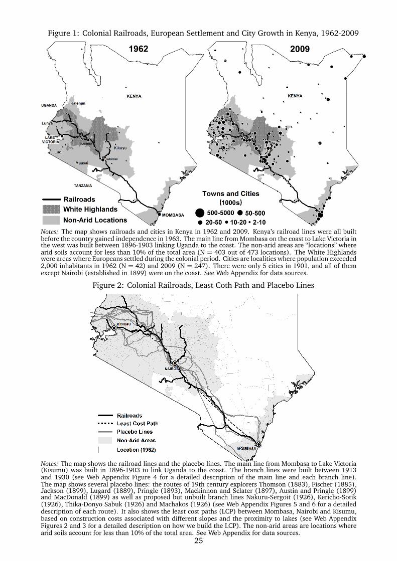
Figure 1: Colonial Railroads, European Settlement and City Growth in Kenya, 1962-2009

Notes: The map shows railroads and cities in Kenya in 1962 and 2009. Kenya’s railroad lines were all builtbefore the country gained independence in 1963. The main line from Mombasa on the coast to Lake Victoria inthe west was built between 1896-1903 linking Uganda to the coast. The non-arid areas are “locations” wherearid soils account for less than 10% of the total area (N = 403 out of 473 locations). The White Highlandswere areas where Europeans settled during the colonial period. Cities are localities where population exceeded2,000 inhabitants in 1962 (N = 42) and 2009 (N = 247). There were only 5 cities in 1901, and all of themexcept Nairobi (established in 1899) were on the coast. See Web Appendix for data sources.

Figure 2: Colonial Railroads, Least Coth Path and Placebo Lines

Notes: The map shows the railroad lines and the placebo lines. The main line from Mombasa to Lake Victoria(Kisumu) was built in 1896-1903 to link Uganda to the coast. The branch lines were built between 1913and 1930 (see Web Appendix Figure 4 for a detailed description of the main line and each branch line).The map shows several placebo lines: the routes of 19th century explorers Thomson (1883), Fischer (1885),Jackson (1899), Lugard (1889), Pringle (1893), Mackinnon and Sclater (1897), Austin and Pringle (1899)and MacDonald (1899) as well as proposed but unbuilt branch lines Nakuru-Sergoit (1926), Kericho-Sotik(1926), Thika-Donyo Sabuk (1926) and Machakos (1926) (see Web Appendix Figures 5 and 6 for a detaileddescription of each route). It also shows the least cost paths (LCP) between Mombasa, Nairobi and Kisumu,based on construction costs associated with different slopes and the proximity to lakes (see Web AppendixFigures 2 and 3 for a detailed description on how we build the LCP). The non-arid areas are locations wherearid soils account for less than 10% of the total area. See Web Appendix for data sources.

25

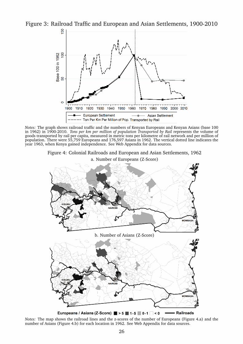
Figure 3: Railroad Traffic and European and Asian Settlements, 1900-2010

Notes: The graph shows railroad traffic and the numbers of Kenyan Europeans and Kenyan Asians (base 100in 1962) in 1900-2010. Tons per km per million of population Transported by Rail represents the volume ofgoods transported by rail per capita, measured in metric tons per kilometre of rail network and per million ofpopulation. There were 55,759 Europeans and 176,597 Asians in 1962. The vertical dotted line indicates theyear 1963, when Kenya gained independence. See Web Appendix for data sources.

Figure 4: Colonial Railroads and European and Asian Settlements, 1962a. Number of Europeans (Z-Score)

b. Number of Asians (Z-Score)

Notes: The map shows the railroad lines and the z-scores of the number of Europeans (Figure 4.a) and thenumber of Asians (Figure 4.b) for each location in 1962. See Web Appendix for data sources.

26

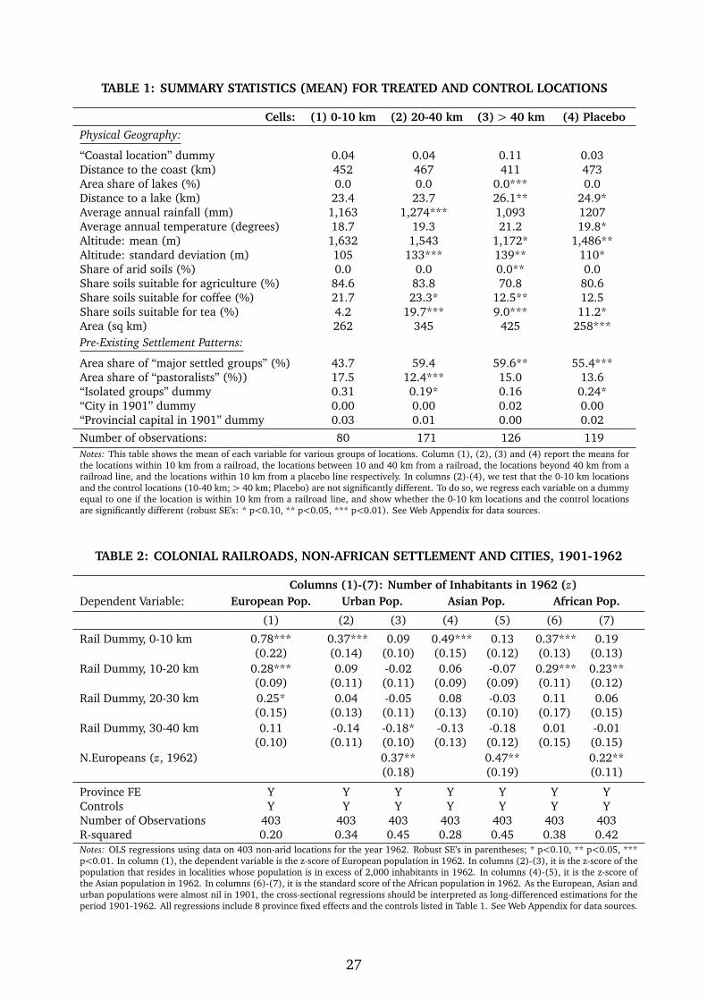
TABLE 1: SUMMARY STATISTICS (MEAN) FOR TREATED AND CONTROL LOCATIONS

Cells: (1) 0-10 km (2) 20-40 km (3) > 40 km (4) Placebo

Physical Geography:

“Coastal location” dummy 0.04 0.04 0.11 0.03Distance to the coast (km) 452 467 411 473Area share of lakes (%) 0.0 0.0 0.0*** 0.0Distance to a lake (km) 23.4 23.7 26.1** 24.9*Average annual rainfall (mm) 1,163 1,274*** 1,093 1207Average annual temperature (degrees) 18.7 19.3 21.2 19.8*Altitude: mean (m) 1,632 1,543 1,172* 1,486**Altitude: standard deviation (m) 105 133*** 139** 110*Share of arid soils (%) 0.0 0.0 0.0** 0.0Share soils suitable for agriculture (%) 84.6 83.8 70.8 80.6Share soils suitable for coffee (%) 21.7 23.3* 12.5** 12.5Share soils suitable for tea (%) 4.2 19.7*** 9.0*** 11.2*Area (sq km) 262 345 425 258***Pre-Existing Settlement Patterns:

Area share of “major settled groups” (%) 43.7 59.4 59.6** 55.4***Area share of “pastoralists” (%)) 17.5 12.4*** 15.0 13.6“Isolated groups” dummy 0.31 0.19* 0.16 0.24*“City in 1901” dummy 0.00 0.00 0.02 0.00“Provincial capital in 1901” dummy 0.03 0.01 0.00 0.02

Number of observations: 80 171 126 119Notes: This table shows the mean of each variable for various groups of locations. Column (1), (2), (3) and (4) report the means forthe locations within 10 km from a railroad, the locations between 10 and 40 km from a railroad, the locations beyond 40 km from arailroad line, and the locations within 10 km from a placebo line respectively. In columns (2)-(4), we test that the 0-10 km locationsand the control locations (10-40 km; > 40 km; Placebo) are not significantly different. To do so, we regress each variable on a dummyequal to one if the location is within 10 km from a railroad line, and show whether the 0-10 km locations and the control locationsare significantly different (robust SE’s: * p<0.10, ** p<0.05, *** p<0.01). See Web Appendix for data sources.

TABLE 2: COLONIAL RAILROADS, NON-AFRICAN SETTLEMENT AND CITIES, 1901-1962

Columns (1)-(7): Number of Inhabitants in 1962 (z)Dependent Variable: European Pop. Urban Pop. Asian Pop. African Pop.

(1) (2) (3) (4) (5) (6) (7)

Rail Dummy, 0-10 km 0.78*** 0.37*** 0.09 0.49*** 0.13 0.37*** 0.19(0.22) (0.14) (0.10) (0.15) (0.12) (0.13) (0.13)

Rail Dummy, 10-20 km 0.28*** 0.09 -0.02 0.06 -0.07 0.29*** 0.23**(0.09) (0.11) (0.11) (0.09) (0.09) (0.11) (0.12)

Rail Dummy, 20-30 km 0.25* 0.04 -0.05 0.08 -0.03 0.11 0.06(0.15) (0.13) (0.11) (0.13) (0.10) (0.17) (0.15)

Rail Dummy, 30-40 km 0.11 -0.14 -0.18* -0.13 -0.18 0.01 -0.01(0.10) (0.11) (0.10) (0.13) (0.12) (0.15) (0.15)

N.Europeans (z, 1962) 0.37** 0.47** 0.22**(0.18) (0.19) (0.11)

Province FE Y Y Y Y Y Y YControls Y Y Y Y Y Y YNumber of Observations 403 403 403 403 403 403 403R-squared 0.20 0.34 0.45 0.28 0.45 0.38 0.42Notes: OLS regressions using data on 403 non-arid locations for the year 1962. Robust SE’s in parentheses; * p<0.10, ** p<0.05, ***p<0.01. In column (1), the dependent variable is the z-score of European population in 1962. In columns (2)-(3), it is the z-score of thepopulation that resides in localities whose population is in excess of 2,000 inhabitants in 1962. In columns (4)-(5), it is the z-score ofthe Asian population in 1962. In columns (6)-(7), it is the standard score of the African population in 1962. As the European, Asian andurban populations were almost nil in 1901, the cross-sectional regressions should be interpreted as long-differenced estimations for theperiod 1901-1962. All regressions include 8 province fixed effects and the controls listed in Table 1. See Web Appendix for data sources.

27

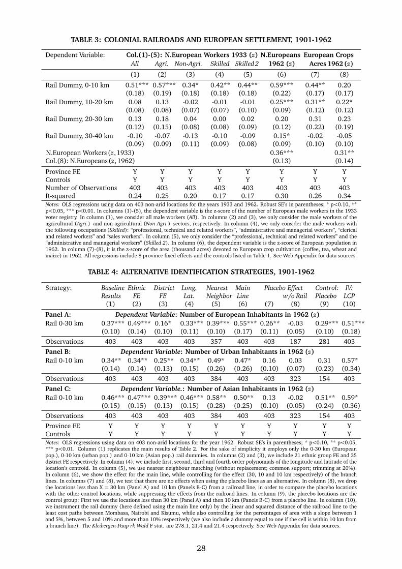
TABLE 3: COLONIAL RAILROADS AND EUROPEAN SETTLEMENT, 1901-1962

Dependent Variable: Col.(1)-(5): N.European Workers 1933 (z) N.Europeans European CropsAll Agri. Non-Agri. Skilled Skilled2 1962 (z) Acres 1962 (z)

(1) (2) (3) (4) (5) (6) (7) (8)

Rail Dummy, 0-10 km 0.51*** 0.57*** 0.34* 0.42** 0.44** 0.59*** 0.44** 0.20(0.18) (0.19) (0.18) (0.18) (0.18) (0.22) (0.17) (0.17)

Rail Dummy, 10-20 km 0.08 0.13 -0.02 -0.01 -0.01 0.25*** 0.31** 0.22*(0.08) (0.08) (0.07) (0.07) (0.10) (0.09) (0.12) (0.12)

Rail Dummy, 20-30 km 0.13 0.18 0.04 0.00 0.02 0.20 0.31 0.23(0.12) (0.15) (0.08) (0.08) (0.09) (0.12) (0.22) (0.19)

Rail Dummy, 30-40 km -0.10 -0.07 -0.13 -0.10 -0.09 0.15* -0.02 -0.05(0.09) (0.09) (0.11) (0.09) (0.08) (0.09) (0.10) (0.10)

N.European Workers (z,1933) 0.36*** 0.31**Col.(8): N.Europeans(z,1962) (0.13) (0.14)

Province FE Y Y Y Y Y Y Y YControls Y Y Y Y Y Y Y YNumber of Observations 403 403 403 403 403 403 403 403R-squared 0.24 0.25 0.20 0.17 0.17 0.30 0.26 0.34Notes: OLS regressions using data on 403 non-arid locations for the years 1933 and 1962. Robust SE’s in parentheses; * p<0.10, **p<0.05, *** p<0.01. In columns (1)-(5), the dependent variable is the z-score of the number of European male workers in the 1933voter registry. In column (1), we consider all male workers (All). In columns (2) and (3), we only consider the male workers of theagricultural (Agri.) and non-agricultural (Non-Agri.) sectors, respectively. In column (4), we only consider the male workers withthe following occupations (Skilled): “professional, technical and related workers”, “administrative and managerial workers”, “clericaland related workers” and “sales workers”. In column (5), we only consider the “professional, technical and related workers” and the“administrative and managerial workers” (Skilled 2). In column (6), the dependent variable is the z-score of European population in1962. In column (7)-(8), it is the z-score of the area (thousand acres) devoted to European crop cultivation (coffee, tea, wheat andmaize) in 1962. All regressions include 8 province fixed effects and the controls listed in Table 1. See Web Appendix for data sources.

TABLE 4: ALTERNATIVE IDENTIFICATION STRATEGIES, 1901-1962

Strategy: Baseline Ethnic District Long. Nearest Main Placebo Effect Control: IV:Results FE FE Lat. Neighbor Line w/o Rail Placebo LCP

(1) (2) (3) (4) (5) (6) (7) (8) (9) (10)

Panel A: Dependent Variable: Number of European Inhabitants in 1962 (z)Rail 0-30 km 0.37*** 0.49*** 0.16* 0.33*** 0.39*** 0.55*** 0.26** -0.03 0.29*** 0.51***

(0.10) (0.14) (0.10) (0.11) (0.10) (0.17) (0.11) (0.05) (0.10) (0.18)

Observations 403 403 403 403 357 403 403 187 281 403

Panel B: Dependent Variable: Number of Urban Inhabitants in 1962 (z)Rail 0-10 km 0.34** 0.34** 0.25** 0.34** 0.49* 0.47* 0.16 0.03 0.31 0.57*

(0.14) (0.14) (0.13) (0.15) (0.26) (0.26) (0.10) (0.07) (0.23) (0.34)

Observations 403 403 403 403 384 403 403 323 154 403

Panel C: Dependent Variable.: Number of Asian Inhabitants in 1962 (z)Rail 0-10 km 0.46*** 0.47*** 0.39*** 0.46*** 0.58** 0.50** 0.13 -0.02 0.51** 0.59*

(0.15) (0.15) (0.13) (0.15) (0.28) (0.25) (0.10) (0.05) (0.24) (0.36)

Observations 403 403 403 403 384 403 403 323 154 403

Province FE Y Y Y Y Y Y Y Y Y YControls Y Y Y Y Y Y Y Y Y YNotes: OLS regressions using data on 403 non-arid locations for the year 1962. Robust SE’s in parentheses; * p<0.10, ** p<0.05,*** p<0.01. Column (1) replicates the main results of Table 2. For the sake of simplicity it employs only the 0-30 km (Europeanpop.), 0-10 km (urban pop.) and 0-10 km (Asian pop.) rail dummies. In columns (2) and (3), we include 21 ethnic group FE and 35district FE respectively. In column (4), we include first, second, third and fourth order polynomials of the longitude and latitude of thelocation’s centroid. In column (5), we use nearest neighbour matching (without replacement; common support; trimming at 20%).In column (6), we show the effect for the main line, while controlling for the effect (30, 10 and 10 km respectively) of the branchlines. In columns (7) and (8), we test that there are no effects when using the placebo lines as an alternative. In column (8), we dropthe locations less than X = 30 km (Panel A) and 10 km (Panels B-C) from a railroad line, in order to compare the placebo locationswith the other control locations, while suppressing the effects from the railroad lines. In column (9), the placebo locations are thecontrol group: First we use the locations less than 30 km (Panel A) and then 10 km (Panels B-C) from a placebo line. In column (10),we instrument the rail dummy (here defined using the main line only) by the linear and squared distance of the railroad line to theleast cost paths between Mombasa, Nairobi and Kisumu, while also controlling for the percentages of area with a slope between 1and 5%, between 5 and 10% and more than 10% respectively (we also include a dummy equal to one if the cell is within 10 km froma branch line). The Kleibergen-Paap rk Wald F stat. are 278.1, 21.4 and 21.4 respectively. See Web Appendix for data sources.

28

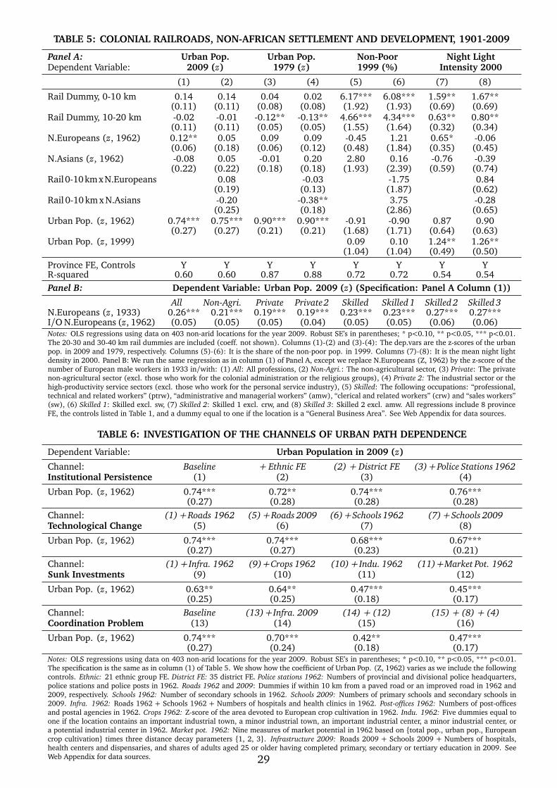
TABLE 5: COLONIAL RAILROADS, NON-AFRICAN SETTLEMENT AND DEVELOPMENT, 1901-2009

Panel A: Urban Pop. Urban Pop. Non-Poor Night LightDependent Variable: 2009 (z) 1979 (z) 1999 (%) Intensity 2000

(1) (2) (3) (4) (5) (6) (7) (8)

Rail Dummy, 0-10 km 0.14 0.14 0.04 0.02 6.17*** 6.08*** 1.59** 1.67**(0.11) (0.11) (0.08) (0.08) (1.92) (1.93) (0.69) (0.69)

Rail Dummy, 10-20 km -0.02 -0.01 -0.12** -0.13** 4.66*** 4.34*** 0.63** 0.80**(0.11) (0.11) (0.05) (0.05) (1.55) (1.64) (0.32) (0.34)

N.Europeans (z, 1962) 0.12** 0.05 0.09 0.09 -0.45 1.21 0.65* -0.06(0.06) (0.18) (0.06) (0.12) (0.48) (1.84) (0.35) (0.45)

N.Asians (z, 1962) -0.08 0.05 -0.01 0.20 2.80 0.16 -0.76 -0.39(0.22) (0.22) (0.18) (0.18) (1.93) (2.39) (0.59) (0.74)

Rail0-10kmxN.Europeans 0.08 -0.03 -1.75 0.84(0.19) (0.13) (1.87) (0.62)

Rail 0-10 km x N.Asians -0.20 -0.38** 3.75 -0.28(0.25) (0.18) (2.86) (0.65)

Urban Pop. (z, 1962) 0.74*** 0.75*** 0.90*** 0.90*** -0.91 -0.90 0.87 0.90(0.27) (0.27) (0.21) (0.21) (1.68) (1.71) (0.64) (0.63)

Urban Pop. (z, 1999) 0.09 0.10 1.24** 1.26**(1.04) (1.04) (0.49) (0.50)

Province FE, Controls Y Y Y Y Y Y Y YR-squared 0.60 0.60 0.87 0.88 0.72 0.72 0.54 0.54Panel B: Dependent Variable: Urban Pop. 2009 (z) (Specification: Panel A Column (1))

All Non-Agri. Private Private2 Skilled Skilled 1 Skilled 2 Skilled 3N.Europeans (z, 1933) 0.26*** 0.21*** 0.19*** 0.19*** 0.23*** 0.23*** 0.27*** 0.27***I/O N.Europeans (z, 1962) (0.05) (0.05) (0.05) (0.04) (0.05) (0.05) (0.06) (0.06)Notes: OLS regressions using data on 403 non-arid locations for the year 2009. Robust SE’s in parentheses; * p<0.10, ** p<0.05, *** p<0.01.The 20-30 and 30-40 km rail dummies are included (coeff. not shown). Columns (1)-(2) and (3)-(4): The dep.vars are the z-scores of the urbanpop. in 2009 and 1979, respectively. Columns (5)-(6): It is the share of the non-poor pop. in 1999. Columns (7)-(8): It is the mean night lightdensity in 2000. Panel B: We run the same regression as in column (1) of Panel A, except we replace N.Europeans (Z, 1962) by the z-score of thenumber of European male workers in 1933 in/with: (1) All: All professions, (2) Non-Agri.: The non-agricultural sector, (3) Private: The privatenon-agricultural sector (excl. those who work for the colonial administration or the religious groups), (4) Private 2: The industrial sector or thehigh-productivity service sectors (excl. those who work for the personal service industry), (5) Skilled: The following occupations: “professional,technical and related workers” (ptrw), “administrative and managerial workers” (amw), “clerical and related workers” (crw) and “sales workers”(sw), (6) Skilled 1: Skilled excl. sw, (7) Skilled 2: Skilled 1 excl. crw, and (8) Skilled 3: Skilled 2 excl. amw. All regressions include 8 provinceFE, the controls listed in Table 1, and a dummy equal to one if the location is a “General Business Area”. See Web Appendix for data sources.

TABLE 6: INVESTIGATION OF THE CHANNELS OF URBAN PATH DEPENDENCE

Dependent Variable: Urban Population in 2009 (z)

Channel: Baseline + Ethnic FE (2) + District FE (3)+ Police Stations 1962Institutional Persistence (1) (2) (3) (4)

Urban Pop. (z, 1962) 0.74*** 0.72** 0.74*** 0.76***(0.27) (0.28) (0.28) (0.28)

Channel: (1)+Roads 1962 (5)+Roads 2009 (6)+Schools1962 (7)+ Schools 2009Technological Change (5) (6) (7) (8)

Urban Pop. (z, 1962) 0.74*** 0.74*** 0.68*** 0.67***(0.27) (0.27) (0.23) (0.21)

Channel: (1)+ Infra. 1962 (9)+Crops 1962 (10)+ Indu. 1962 (11)+Market Pot. 1962Sunk Investments (9) (10) (11) (12)

Urban Pop. (z, 1962) 0.63** 0.64** 0.47*** 0.45***(0.25) (0.25) (0.18) (0.17)

Channel: Baseline (13)+ Infra. 2009 (14) + (12) (15) + (8) + (4)Coordination Problem (13) (14) (15) (16)

Urban Pop. (z, 1962) 0.74*** 0.70*** 0.42** 0.47***(0.27) (0.24) (0.18) (0.17)

Notes: OLS regressions using data on 403 non-arid locations for the year 2009. Robust SE’s in parentheses; * p<0.10, ** p<0.05, *** p<0.01.The specification is the same as in column (1) of Table 5. We show how the coefficient of Urban Pop. (Z, 1962) varies as we include the followingcontrols. Ethnic: 21 ethnic group FE. District FE: 35 district FE. Police stations 1962: Numbers of provincial and divisional police headquarters,police stations and police posts in 1962. Roads 1962 and 2009: Dummies if within 10 km from a paved road or an improved road in 1962 and2009, respectively. Schools 1962: Number of secondary schools in 1962. Schools 2009: Numbers of primary schools and secondary schools in2009. Infra. 1962: Roads 1962 + Schools 1962 + Numbers of hospitals and health clinics in 1962. Post-offices 1962: Numbers of post-officesand postal agencies in 1962. Crops 1962: Z-score of the area devoted to European crop cultivation in 1962. Indu. 1962: Five dummies equal toone if the location contains an important industrial town, a minor industrial town, an important industrial center, a minor industrial center, ora potential industrial center in 1962. Market pot. 1962: Nine measures of market potential in 1962 based on {total pop., urban pop., Europeancrop cultivation} times three distance decay parameters {1, 2, 3}. Infrastructure 2009: Roads 2009 + Schools 2009 + Numbers of hospitals,health centers and dispensaries, and shares of adults aged 25 or older having completed primary, secondary or tertiary education in 2009. SeeWeb Appendix for data sources. 29