arX

iv:0

708.

1399

v2 [

hep-

th]

8 O

ct 2

007

Preprint typeset in JHEP style - HYPER VERSION

Higher Spin Gauge Fields Interacting with

Scalars: The Lagrangian Cubic Vertex

Angelos Fotopoulos

Dipartimento di Fisica Teorica dell’Universita di Torino and INFN

Sezione di Torino, via P. Giuria 1, I-10125 Torino, Italy

Nikos Irges, Anastasios C. Petkou and Mirian Tsulaia

Department of Physics, University of Crete, 71003 Heraklion, Crete, Greece

Abstract: We apply a recently presented BRST procedure to construct the Largangian cubic

vertex of higher-spin gauge field triplets interacting with massive free scalars. In flat space,

the spin-s triplet propagates the series of irreducible spin-s, s − 2,..,0/1 modes which couple

independently to corresponding conserved currents constructed from the scalars. The simple

covariantization of the flat space results is not enough in AdS, as new interaction vertices appear.

We present in detail the cases of spin-2 and spin-3 triplets coupled to scalars. Restricting to

a single irreducible spin-s mode we uncover previously obtained results. We also present an

alternative derivation of the lower spin results based on the idea that higher-spin gauge fields

arise from the gauging of higher derivative symmetries of free matter Lagrangians. Our results

can be readily applied to holographic studies of higher-spin gauge theories.

Contents

1. Introduction 2

2. The BRST approach to the HS cubic vertex 3

3. The cubic vertex in flat space 5

4. The cubic vertex in AdS 7

5. Explicit examples 8

5.1 Spin-2 with two scalars 8

5.2 Spin-3 with two scalars 10

6. Irreducible HS gauge field coupled to scalars in AdS 11

7. An alternative derivation of the cubic couplings 12

7.1 Free massive scalars coupled to the spin-2 triplet 12

7.2 Free massive scalars coupled to the spin-3 triplet 13

8. Summary and Outlook 15

A. Basic Definitions 16

A.1 Definition of |V 〉 and |W 〉 16

B.2 Definition of the F, G functions and their properties 17

C. Commutation relations 19

D. Equations for I3 22

E. The vertex for an irreducible HS gauge field 22

– 1 –

1. Introduction

Constructing consistent interactions for higher-spin (HS) gauge fields is an old problem (see [1]

for recent reviews). A crucial step for its resolution in AdS spaces was taken some years ago by

Fradkin and Vasiliev [2] (see also [3]). Since then, the study of HS gauge theories has enjoyed a

remarkable renaissance and a wealth of new and interesting results have appeared [4]–[20] (see

also [21]– [25] for the earlier work).

One of the approaches to the interaction of HS gauge fields is based on the BRST-like methods

( see e.g., [26] for a review). This is particularly appealing as it resembles similar constructions

in string field theory [27]– [28]. In particular a model of interacting massless HS gauge fields

can be obtained using a cubic vertex of the open string theory [29]. However in the general case

of interacting massless HS fields there is no analog of overlap conditions such as that is present

in the Open String Field Theory and therefore one has to consider a general polynomial of the

corresponding matter and ghost oscillators.

In [30] a systematic method for the construction of the general cubic coupling of any three

HS gauge fields in flat and AdS spaces based on the triplet construction [31]–[33] was presented.

In the present note we apply our method to the simplest case; the interaction between one HS

triplet and two massive free scalars. Despite its apparent simplicity this is still a highly non-

trivial case since it requires the construction of an infinite number of conserved currents, made

out of scalars, that couple properly to HS gauge fields. This is also an important case since, as

we will see in Section 7, it elucidates the emergence of HS gauge fields via the gauging of higher

derivative symmetries of free matter Lagrangians (see [34] for the discussion about self-adjoint

operators in the gauging of HS symmetries). In a holographic setting, our results imply the

existence of an infinite set of Ward identities involving scalar operators in boundary CFTs that

are dual to HS gauge theories in AdS spaces.

The paper is organized as follows:

In Section 2 we briefly review our general method of constructing free and interacting La-

grangians for HS gauge fields [30]–[32]. In Section 3 we present the general result for the La-

grangian cubic interaction vertices between one triplet and two massive free scalars in flat space.

We note the emergence of a pattern; the irreducible spin-s, s − 2, ..., 0/1 modes propagated by

the spin-s triplet couple independently to corresponding conserved currents constructed from

the scalars. In Section 4 we outline how we obtain the general result for AdS. The simple flat

space pattern is no more valid and new interaction vertices appear at order 1/L2. To keep our

presentation clear we relegate the explicit lengthy expressions in the Appendix. In Section 5 we

present the explicit formulae for the spin-2 and spin-3 cases in flat and AdS spaces. In Section 6

we present the results for the cubic vertex of irreducible HS gauge fields interacting with massive

free scalars and show that our formulae reproduce known past results [35]–[37]. Extensive discus-

sions of conformal HS currents were presented also in [36, 38, 39]. In Section 7 we re-derive the

spin-2 and spin-3 vertices in flat and AdS spaces by an alternative method based on the idea that

HS gauge fields arise from the gauging of high derivative symmetries of free matter Lagrangians

[40]–[41]. This procedure opens up the possibility for explicit study of the HS gauge symmetry

– 2 –

acting on scalars, however we leave this interesting idea for a future work. Section 8 contains a

summary and the outlook of our work. Important notation and some lengthy formulae appear

in the five Appendices.

2. The BRST approach to the HS cubic vertex

In this Section we review the BRST approach to constructing the cubic interaction of HS gauge

fields. More details can be found in [32], [30]. We consider an AdS space with radius RAdS = L;

the corresponding equations for flat space are simply obtained by setting the AdS curvature to

zero.

The full interacting Lagrangian can be written as [27] – [28]

L =∑

i=1,2,3

∫

dci0〈Φi|Qi |Φi〉 + g(

∫

dc10dc2

0dc30〈Φ1|〈Φ2|〈Φ3||V 〉 + h.c) , (2.1)

where |V 〉 is the cubic vertex and g is a dimensionless coupling constant.1 To describe the cubic

interaction of HS gauge fields we introduced three vectors |Φi〉 (i = 1, 2, 3) associated to three -

generally different - Fock spaces spanned by the oscillators

[αiµ, αj,+

ν ] = δijgµν , {ci,+, bj} = {ci, bj,+} = {ci0, b

j0} = δij . (2.2)

The vacuum in each one of the Fock spaces is defined as

c|0〉 = 0 , b|0〉 = 0 , b0|0〉 = 0 , αµ|0〉 = 0 . (2.3)

Each of the fields |Φi〉 (so called ”triplets”) has the form

|Φ〉 = |φ〉 + c+ b+ |D〉 + c0 b+ |C〉 , (2.4)

with

|φ〉 =1

s!hµ1...µs

(x)αµ1+ . . . αµs+ |0〉, (2.5)

|D〉 =1

(s − 2)!Dµ1...µs−2

(x)αµ1+ . . . αµs−2+ |0〉 , (2.6)

|C〉 =−i

(s − 1)!Cµ1...µs−1

(x)αµ1+ . . . αµs−1+ |0〉 (2.7)

and the identically nilpotent BRST charge [32] in each of the Fock spaces has the form

Q = c0

(

l0 +1

L2(N2 − 6N + 6 + D − D2

4− 4M+M + c+b(4N − 6)

+b+c(4N − 6) + 12c+bb+c − 8c+b+M + 8M+bc))

+c+l + cl+ − c+cb0 (2.8)

1Each term in the Lagrangian (2.1) has length dimension −D. This requirement holds true for each space-

time vertex contained in (2.1) after multiplication by an appropriate power of the length scale of the theory, as

discussed in [30].

– 3 –

with

l0 = gµνpµpν , l = αµpµ, l+ = αµ+pµ , (2.9)

and

N = αµ+αµ +D2

, M =1

2αµαµ . (2.10)

The momentum operator pµ is defined as [42]

pµ = − i(

∇µ + ωabµ α+

a α b

)

, αa = eaµα

µ , (2.11)

where eaµ and ωab

µ are the vierbein and the spin connection of AdS and ∇µ is the AdS covariant

derivative. The Lagrangian is invariant up to terms of order g2 under the nonabelian gauge

transformations

δ|Φi〉 = Qi|Λi〉 − g

∫

dci+10 dci+2

0 [(〈Φi+1|〈Λi+2| + 〈Φi+2|〈Λi+1|)|V 〉] + O(g2) , (2.12)

with gauge transformation parameters

|Λi〉 = bi,+|λi〉 =i

(s − 1)!λi

µ1µ2...µs−1(x)αi,µ1+αi,µ2+...αi,µs−1+b+|0〉 , (2.13)

provided that the vertex satisfies the BRST invariance condition

Q|V 〉 = 0 , Q =∑

i

Qi. (2.14)

The vertex operator |V 〉 has ghost number +3 and its structure is

|V 〉 = V |−〉123, |−〉123 = c10c

20c

30 |0〉1 ⊗ |0〉2 ⊗ |0〉3 , (2.15)

where V is an unknown function of the rest of the oscillators with ghost number zero. Note that

equation (2.14) determines the vertex up to Q-exact terms

δ|V 〉 = Q|W 〉 , (2.16)

where |W 〉 is an operator with total ghost number +2. The BRST-exact terms correspond to

the ones which can be obtained by field redefinitions from the free Lagrangian. To simplify the

analysis of equation (2.14) we define the operator

N = αµ,i+αiµ + bi,+ci + ci,+bi . (2.17)

This operator commutes with the BRST charges Qi. This means that the vertex can be expanded

in a sum of terms, each with fixed eigenvalues K of the operator N as

|V 〉 =∑

K

|V (K)〉 . (2.18)

Therefore, equation (2.14) can be split into the set of algebraic equations∑

i

QiV (K) = 0 (2.19)

for each value of K. The systematic solution of these equations determines the type the of cubic

vertex.

– 4 –

3. The cubic vertex in flat space

In this section we will use our general approach to construct the cubic coupling of an HS triplet

with two scalars in flat space. The corresponding coupling for irreducible HS fields has been

discussed [44] and more recently in [35, 37]. The merit of considering the triplet is twofold.

Firstly, our general BRST construction is systematic, can be straightforwardly generalized to

AdSD and is relevant for string field theory constructions. Secondly, our construction gives rise

to the idea that HS gauge fields arise from the gauging of higher derivative symmetries of free

matter Lagrangians.

To proceed, we put the triplet of spin s in Fock space 3 and the two scalars φ1 and φ2 into

Fock spaces 1 and 2. Therefore, the matter and complex ghost oscillators appear only in Fock

space 3. This allows us to write down the most general polynomial in terms of the expansion in

ghost variables as (see Appendix A for the definition of the various operators used below)

〈V | = 123〈−|{

X1 + X233γ

33 + X33jβ

3j}

, j = 1, 2, 3 , (3.1)

where

X1 = X1n1,n2,n3;m3,k3;p3, (l10)

n1(l20)n2(l20)

n3(l3)m3(I3)k3(M33)p3 , (3.2)

and with the same expansions for the coefficients X233 and X3

3j . We will apply the field redefinition

(FR) scheme outlined in [30] in order to eliminate the li0 from all three matrix elements, and

the l3 dependence from X1 and X2. This amounts to removing the indices n1, n2, n3 from the

expressions of X1, X233 and X3

3j . Then, the BRST invariance condition (2.14) simplifies to

123〈−|(I3)k3 (l33)

m3 (M33)p3

[

−X331;k3,m3,p3

l110 − X332;k3,n3,p3

l220 −

X333;k3,n3,p3

l330 + δm3,0(l+33 X1

k3,0,p3− l33 X2

33;k3,0,p3)]

= 0 . (3.3)

We can solve (3.3) to derive

X331;0,k3−1,p3

= k3X10,k3,p3

,

X332;0,k3−1,p3

= −k3X10,k3,p3

,

X233;0,k3,p3−1 = −p3X

10,k3,p3

,

X333;m3,k3,p3

= 0 ,

X3ij;m3 6=0;k3,p3

= X333;m3 6=0;k3,p3

= X1m3 6=0;k3,p3

= 0 . (3.4)

For a triplet of spin-s the solution takes the form (we drop the m3 index from now on):

〈V | = 123〈−|{

X1k3,p3

− (p3 + 1)X1k3,p3+1γ

33,+

+(k3 + 1)X1k3+1,p3

β31,+ − (k3 + 1)X1k3+1,p3

β32,+}

(I+,3)k3(M+,33)p3 , (3.5)

with

s = 2p3 + k3, X1k3,p3

= 2p3 Cs,p3

k3 = 0, 1, .., s . (3.6)

– 5 –

Using the ”momentum conservation” condition p1µ + p2

µ + p3µ = 0 and the solution above we can

write the gauge transformation rules for scalars (2.12) in the form

δφa = g

[ s−12

]∑

p=0

ξab (s − 2p) Cs,p

s−1−2p∑

r=0

(

s − 1 − 2p

r

)

2r

(∂µr+1 . . . ∂µs−1−2pλ[p]µ1...µs−1−2p

) (∂µ1 . . . ∂µrφb) (3.7)

ξ12 = (−1)s−1ξ21 = −1, ξ11 = ξ22 = 0 a, b = 1, 2 , (3.8)

where Cs,p are arbitrary parameters. Note that the gauge transformations of the scalars are

nonabelian, whereas the gauge transformations of the fields in the spin-s triplet remain abelian

δhµ1...µs= ∂{µ1

λµ2...µs}, δCµ1...µs−1= 2λµ1...µs

, δDµ1...µs−2= ∂µλµ,µ1...µs−2

.. (3.9)

At this point we should emphasize that we have not imposed any symmetry between the scalars

φa. It is obvious though from (3.8) that for HS triplets with s odd (s = 2k + 1) one needs at

least two different real scalars (or alternatively one complex scalar) to have a non-zero coupling2. The simple example of this is the s = 1 case where we find linearized scalar electrodynamics.

For even s HS triplets (s = 2k) the condition (3.8) gives no obstruction to coupling with a single

real scalar.

Finally, after some rather lengthy rearrangement we obtain the cubic interaction terms in

the Lagrangian as

Ls00 =

∫

ddx{

[ s2]

∑

p=0

Cs,p W [p]µ1...µs−2p

×

s−2p∑

r=0

(

s − 2p

r

)

(−1)r (∂µ1 . . . ∂µrφ1) (∂µr+1 . . . ∂µs−2pφ2) + h.c.}

=

∫

ddx

[ s2]

∑

p=0

Cs,p Wp · Js−2p + h.c. , (3.10)

where we have used the binomial coefficients

(

n

m

)

and [ s2] is the integer part of s

2. Wp is defined

in [31]

Wp = h[p] − 2p D[p−1] , δWp = ∂Λ[p] , (3.11)

and

Js−2p =

s−2p∑

r=0

(

s − 2p

r

)

(−1)r (∂µ1 . . . ∂µrφ1) (∂µr+1 . . . ∂µs−2pφ2) . (3.12)

2Indeed setting φ1 = φ2 in (3.7) and taking into account (3.8) leads into an inconsitency for s-odd while it is

allowed for s-even.

– 6 –

The fields Wp define a chain of lower spin fields contained in the triplet as can easily be seen from

their gauge transformation properties (3.11). They are rank s−2p symmetric tensors. Hence, the

currents of (3.12) are also symmetrized and by virtue of the transformation properties (3.11) are

conserved. We see a pattern emerging: given a general free scalar Lagrangian we can construct

the series of spin-s, s − 2, ..., 0/1 symmetric conserved currents (3.12) that couple properly to a

spin-s triplet. In Section 7 we will try to understand the deep reason for the existence of such

currents.

4. The cubic vertex in AdS

In this section we present the construction of the cubic vertex of a triplet coupled to two massive

free scalars in AdS space. In this case the calculations are rather more involved, nevertheless we

will be able to obtain a relatively simple result for the vertex.

The vertex still has the form (3.1). Next, we choose an FR (field redefinition) scheme where

one can eliminate all lii0 dependence in (A.3) and set X333 = 0 in (3.1). With this choice we are

able to eliminate any li dependence from X233. Therefore one has the expansion of the vertex

〈V | = 123〈−|(I3)k3 (l33)

m3 (M33)p3

{

X1k3,m3,p3

+ X233;k3,0,p3

γ33

+ X331;k3,m3,p3

β13 + X332;k3,m3,p3

β23}

. (4.1)

The BRST invariance gives the equation

123〈−|(I3)k3 (l33)

m3 (M33)p3

{

−X331;k3,m3,p3

(l110 − 2D − 6

L2) − (4.2)

X332;k3,m3,p3

(l220 − 2D − 6

L2) + l+33X

1k3,m3,p3

− l33δm3,0X233;k3,0,p3

}

= 0 .

In order to arrive at the equivalent of (3.4) we will have to commute all creation operators α+,3µ to

the left but we will also have to eliminate one of the three momenta i.e., pµ,3 using ”momentum

conservation”. In flat space commutativity of momenta makes this a very easy task. In AdS this

becomes rather involved due to the relation (C.1) (see also [30]). The rules one should apply are

the following3:

• In order to use ”momentum conservation” we move the operators pµ3 to the far left of the

expression. Then we substitute pµ1 + pµ

2 + pµ3 = 0. For example, instead of writing

(l32)pρ,3(l32)pρ2 = pρ,3(l32)(l32)p

ρ2 , (4.3)

which translates to∫

dDx√−g(∇ρΛµν)(∇µ∇ν∇ρφ

2)φ1 (4.4)

3We set L2 = 1 in what follows and restore it at the end by dimensional analysis.

– 7 –

we use

−(p1µ, + p2

µ)(l32)(l32)pµ2 , (4.5)

which translates into

−∫

dDx√−gΛµν [(∇µ∇ν∇ρφ2)(∇ρφ

1) + (∇ρ∇µ∇ν∇ρφ2)φ1] , . (4.6)

• We will then use the equations of Appendix D to move any ”non-contracted” momenta

piµ, i = 1, 2 to the right until they form operators l110 , l220 , l31 or l32 with operators p1

µ, p2µ or

α3µ. In the present example we should push the operators p1

µ and p2µ to the right until they

form the operators l110 and l120 when combined with pµ2 . This process will generate terms

proportional to 1L2 . For the example above they are

−∫

dDx√−g

1

L2[Λµ

µ(2φ2)φ1 + (1 − 2D)Λµν(∇µ∇νφ2)φ1] (4.7)

which can be seen from the second term in (4.6) when pushing the covariant derivative ∇ρ

to the right.

• We will commute creation oscillators to the left. In doing so we will once more generate

non-contacted momenta pµ,i i = 1, 2 which in turn have to be pushed to the right and will

generate further 1/L2 terms as explained in the previous step.

• Finally the ordering rule is that all operators l110 , l220 which do not commute with I3, and

l3, are to be brought to the extreme right of the equation so that we compare operator

expressions which have the same ordering.

This procedure results in some quite lengthy equations but our choice of FR scheme which

has eliminated X333 simplifies the problem. Actually, we have to perform the manipulations

described above only for the third and fourth terms in (4.2). For the fourth terms we just push

the operator pµ,3 to the left, then use ”momentum conservation” and then push the operator

pµ,1 + pµ,2 to the right as described above. The third term is the hardest one since it requires

performance of commutators both among momenta and among oscillators.

The solution for generic triplet is quite involved but straightforward. In the Appendices

we give some explicit formulae that are used in the manipulations described above. The full

solution for the triplet will not be presented here. Instead, as an illustration of our technique we

present the two simplest examples describing the interaction of spin-2 and spin-3 triplets with

two massive free scalars.

5. Explicit examples

5.1 Spin-2 with two scalars

Since the oscillators αi,+µ , ci,+ and bi,+ occur only in the third Fock space we omit the index i for

them in what follows. The field will will using are

|Φ1〉 = φ1(x)|0〉, |Φ2〉 = φ2(x)|0〉, (5.1)

– 8 –

|Φ3〉 = (1

2!hµν(x)αµ+αν+ + D(x)c+b+ − iCµ(x)αµ+c3

0b+)|0〉 , (5.2)

|Λ〉 = iλµ(x)αµ+b+|0〉 . (5.3)

The Lagrangian has the form

L = Lfree + Lint , (5.4)

Lfree = (∂µφ1)(∂µφ1) + (∂µφ2)(∂

µφ2) + m2(φ21 + φ2

2) + (∂ρhµν)(∂ρhµν)

−4(∂µhµν)Cν − 4(∂µC

µ)D − 2(∂µD)(∂µD) + 2CµCµ , (5.5)

Lint = C2,0 (hµν(∂µ∂νφ1)φ2 + hµν(∂µ∂νφ2)φ1 − 2hµν(∂µφ1)(∂νφ2))

−C2,1 φ1φ2(hµµ − 2D) . (5.6)

The relevant gauge transformations are

δφ1 = C2,0 (2λµ∂µφ2 + φ2∂µλµ) , (5.7)

δφ2 = C2,0 (2λµ∂µφ1 + φ1∂µλµ) , (5.8)

δhµν = ∂µλν + ∂νλµ, δCµ = 2λµ, δD = ∂µλµ . (5.9)

According to our general construction, given in the section 2 we have obtained the cubic vertex

which involves two different scalars and the triplet with higher spin 2. To obtain the interaction

of a single scalar with the spin-2 field we need to set φ1 = φ24. It should also be noticed that

for φ1 = φ2 (5.6) is equivalent to the linearized interaction of a scalar field with gravity as we

explain in Section 7.1. and in particular in equations (7.4) and (7.6). The generalization for

the coupling of a spin-2 triplet with an arbitrary number of scalar fields n goes in an analogous

manner with the constants C2,0 becoming n × n matrices. Similar things apply to the couplings

of scalars with any HS triplet. For simplicity in what follows we will discuss only the two scalar

case which the reader can generalize easily to the n scalar case.

In AdSD we replace ordinary with covariant derivatives. There will be no other changes for

the gauge transformation rules (i.e., for all fields δAdS = δ) (5.9) except for

δAdSCµ = δCµ +1 −D

L2λµ , (5.10)

The free Lagrangian is modified to include the standard AdS ”mass -terms” of order 1/L2

∆Lfree = − 1

L2(2hµ

µhνν − 16hµ

µD + 2hµνhµν + (4D + 12)D2 + (2D − 6) (φ2

1 + φ22)) . (5.11)

The interaction part also changes and gets an additional piece

∆Lint. = C2,0D − 1

L2Dφ1φ2 . (5.12)

This is an additional interaction of the D scalar with a ”spin-0” current.

4Notice that setting i.e. φ2 = 0 is meaningless since in our formalism that would mean to consider two Hilbert

spaces, hence no cubic interaction vertex.

– 9 –

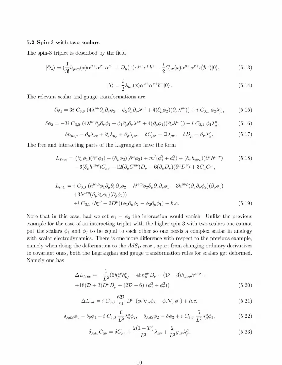
5.2 Spin-3 with two scalars

The spin-3 triplet is described by the field

|Φ3〉 = (1

3!hµνρ(x)αµ+αν+αρ+ + Dµ(x)αµ+c+b+ − i

2Cµν(x)αµ+αν+c3

0b+)|0〉, (5.13)

|Λ〉 =i

2λµν(x)αµ+αν+b+|0〉 . (5.14)

The relevant scalar and gauge transformations are

δφ1 = 3i C3,0 (4λµν∂µ∂νφ2 + φ2∂µ∂νλµν + 4(∂µφ2)(∂νλ

µν)) + i C3,1 φ2λµµ , (5.15)

δφ2 = −3i C3,0 (4λµν∂µ∂νφ1 + φ1∂µ∂νλµν + 4(∂µφ1)(∂νλ

µν)) − i C3,1 φ1λµµ , (5.16)

δhµνρ = ∂µλνρ + ∂νλµρ + ∂ρλµν , δCµν = 2λµν , δDµ = ∂νλνµ . (5.17)

The free and interacting parts of the Lagrangian have the form

Lfree = (∂µφ1)(∂µφ1) + (∂µφ2)(∂

µφ2) + m2(φ21 + φ2

2) + (∂τhµνρ)(∂τhµνρ) (5.18)

−6(∂ρhµνρ)Cµρ − 12(∂µC

µν)Dν − 6(∂µDν)(∂µDν) + 3CµC

µ ,

Lint. = i C3,0 (hµνρφ1∂µ∂ν∂ρφ2 − hµνρφ2∂µ∂ν∂ρφ1 − 3hµνρ(∂µ∂νφ2)(∂ρφ1)

+3hµνρ(∂µ∂νφ1)(∂ρφ2))

+i C3,1 (hµνν − 2Dµ)(φ1∂µφ2 − φ2∂µφ1) + h.c. (5.19)

Note that in this case, had we set φ1 = φ2 the interaction would vanish. Unlike the previous

example for the case of an interacting triplet with the higher spin 3 with two scalars one cannot

put the scalars φ1 and φ2 to be equal to each other so one needs a complex scalar in analogy

with scalar electrodynamics. There is one more difference with respect to the previous example,

namely when doing the deformation to the AdSD case , apart from changing ordinary derivatives

to covariant ones, both the Lagrangian and gauge transformation rules for scalars get deformed.

Namely one has

∆Lfree = − 1

L2(6hµρ

µ hννρ − 48hµν

µ Dν − (D − 3)hµνρhµνρ +

+18(D + 3)DµDµ + (2D − 6) (φ21 + φ2

2)) (5.20)

∆Lint = i C3,06DL2

Dµ (φ1∇µφ2 − φ2∇µφ1) + h.c. (5.21)

δAdSφ1 = δ0φ1 − i C3,06

L2λµ

µφ2, δAdSφ2 = δφ2 + i C3,06

L2λµ

µφ1, (5.22)

δAdSCµν = δCµν +2(1 −D)

L2λµν +

2

L2gµνλ

ρρ. (5.23)

– 10 –

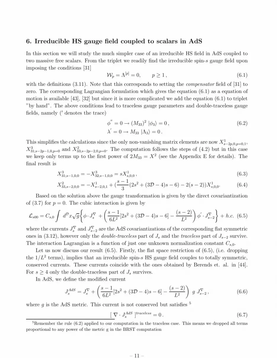
6. Irreducible HS gauge field coupled to scalars in AdS

In this section we will study the much simpler case of an irreducible HS field in AdS coupled to

two massive free scalars. From the triplet we readily find the irreducible spin-s gauge field upon

imposing the conditions [31]

Wp = Λ[p] = 0, p ≥ 1 , (6.1)

with the definitions (3.11). Note that this corresponds to setting the compensator field of [31] to

zero. The corresponding Lagrangian formulation which gives the equation (6.1) as a equation of

motion is available [43], [32] but since it is more complicated we add the equation (6.1) to triplet

”by hand”. The above conditions lead to traceless gauge parameters and double-traceless gauge

fields, namely (′ denotes the trace)

φ′′

= 0 → (M33)2 |φ3〉 = 0 , (6.2)

λ′

= 0 → M33 |Λ3〉 = 0 .

This simplifies the calculations since the only non-vanishing matrix elements are now X1s−2p,0,p=0,1,

X331;s−2p−1,0,p=0 and X2

33;s−2p−2,0,p=0. The computation follows the steps of (4.2) but in this case

we keep only terms up to the first power of 2M33 = X2 (see the Appendix E for details). The

final result is

X331;s−1,0,0 = −X3

32;s−1,0,0 = sX1s,0,0 , (6.3)

X233,s−2,0,0 = −X1

s−2,0,1 + (s − 1

3(2s2 + (3D − 4)s − 6) − 2(s − 2))X1

s,0,0. (6.4)

Based on the solution above the gauge transformation is given by the direct covariantization

of (3.7) for p = 0. The cubic interaction is given by

Ls00 = Cs,0

∫

dDx√

g

{

φ ·J∇s +

(

s − 1

6L2[2s2 + (3D − 4)s − 6] − (s − 2)

L2

)

φ′ ·J∇

s−2

}

+ h.c. (6.5)

where the currents J∇s and J∇

s−2 are the AdS covariantizations of the corresponding flat symmetric

ones in (3.12), however only the double-traceless part of Js and the traceless part of Js−2 survive.

The interaction Lagrangian is a function of just one unknown normalization constant Cs,0.

Let us now discuss our result (6.5). Firstly, the flat space restriction of (6.5), (i.e. dropping

the 1/L2 terms), implies that an irreducible spin-s HS gauge field couples to totally symmetric,

conserved currents. These currents coincide with the ones obtained by Berends et. al. in [44].

For s ≥ 4 only the double-traceless part of Js survives.

In AdS, we define the modified current

JAdSs = J∇

s +

(

s − 1

6L2[2s2 + (3D − 4)s − 6] − (s − 2)

L2

)

g J∇s−2 , (6.6)

where g is the AdS metric. This current is not conserved but satisfies 5

[ ∇ · JAdSs ]traceless = 0 . (6.7)

5Remember the rule (6.2) applied to our computation in the traceless case. This means we dropped all terms

proportional to any power of the metric g in the BRST computation

– 11 –

This condition implies that the covariantized flat spin-s current J∇s fails to be conserved by order

1/L2 terms.

A few more comments are in order here. In flat space, the conserved currents Js are not

the only ones that couple consistently to irreducible HS gauge fields. They can be modified, at

will, by terms whose divergence gives zero upon contraction with the traceless gauge parameter

λ. We fixed this freedom by imposing the conditions (6.1) i.e. setting compensator field to zero.

In [35] an additional single zero trace condition was used for the conserved currents in order to

uniquely fix the form of the higher-spin currents in flat space. This condition was generalized in

AdS by [37]. In the above works, bulk conformal (or Weyl) invariance played a crucial role. We

believe that our approach is more general since our HS gauge fields are coupled generically to

massive scalars. It is also satisfying that our approach is naturally tied to BRST, as we believe

that this is relevant for the application of our results to string theory.

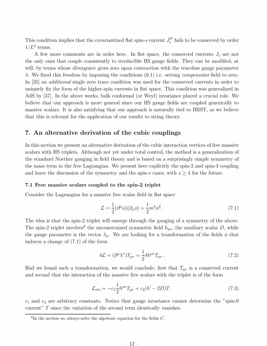
7. An alternative derivation of the cubic couplings

In this section we present an alternative derivation of the cubic interaction vertices of free massive

scalars with HS triplets. Although not yet under total control, the method is a generalization of

the standard Noether gauging in field theory and is based on a surprisingly simple symmetry of

the mass term in the free Lagrangian. We present here explicitly the spin-2 and spin-3 coupling

and leave the discussion of the symmetry and the spin-s cases, with s ≥ 4 for the future.

7.1 Free massive scalars coupled to the spin-2 triplet

Consider the Lagrangian for a massive free scalar field in flat space

L =1

2(∂µφ)(∂µφ) +

1

2m2φ2 . (7.1)

The idea is that the spin-2 triplet will emerge through the gauging of a symmetry of the above.

The spin-2 triplet involves6 the unconstrained symmetric field hµν , the auxiliary scalar D, while

the gauge parameter is the vector λµ. We are looking for a transformation of the fields φ that

induces a change of (7.1) of the form

δL = (∂µλν)Tµν =1

2δhµνTµν . (7.2)

Had we found such a transformation, we would conclude; first that Tµν is a conserved current

and second that the interaction of the massive free scalars with the triplet is of the form

Lint = −c11

2hµνTµν + c2(h

′ − 2D)T . (7.3)

c1 and c2 are arbitrary constants. Notice that gauge invariance cannot determine the ”spin-0

current” T since the variation of the second term identically vanishes.

6In the section we always solve the algebraic equation for the fields C.

– 12 –

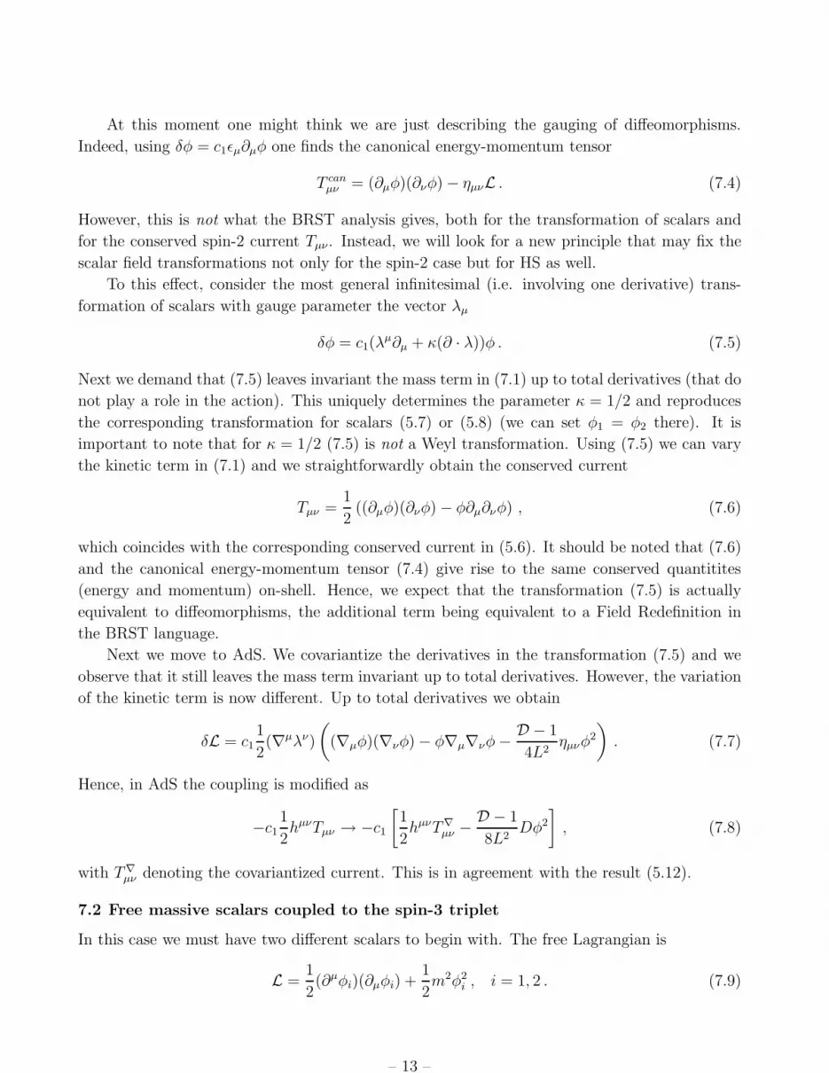
At this moment one might think we are just describing the gauging of diffeomorphisms.

Indeed, using δφ = c1ǫµ∂µφ one finds the canonical energy-momentum tensor

T canµν = (∂µφ)(∂νφ) − ηµνL . (7.4)

However, this is not what the BRST analysis gives, both for the transformation of scalars and

for the conserved spin-2 current Tµν . Instead, we will look for a new principle that may fix the

scalar field transformations not only for the spin-2 case but for HS as well.

To this effect, consider the most general infinitesimal (i.e. involving one derivative) trans-

formation of scalars with gauge parameter the vector λµ

δφ = c1(λµ∂µ + κ(∂ · λ))φ . (7.5)

Next we demand that (7.5) leaves invariant the mass term in (7.1) up to total derivatives (that do

not play a role in the action). This uniquely determines the parameter κ = 1/2 and reproduces

the corresponding transformation for scalars (5.7) or (5.8) (we can set φ1 = φ2 there). It is

important to note that for κ = 1/2 (7.5) is not a Weyl transformation. Using (7.5) we can vary

the kinetic term in (7.1) and we straightforwardly obtain the conserved current

Tµν =1

2((∂µφ)(∂νφ) − φ∂µ∂νφ) , (7.6)

which coincides with the corresponding conserved current in (5.6). It should be noted that (7.6)

and the canonical energy-momentum tensor (7.4) give rise to the same conserved quantitites

(energy and momentum) on-shell. Hence, we expect that the transformation (7.5) is actually

equivalent to diffeomorphisms, the additional term being equivalent to a Field Redefinition in

the BRST language.

Next we move to AdS. We covariantize the derivatives in the transformation (7.5) and we

observe that it still leaves the mass term invariant up to total derivatives. However, the variation

of the kinetic term is now different. Up to total derivatives we obtain

δL = c11

2(∇µλν)

(

(∇µφ)(∇νφ) − φ∇µ∇νφ − D − 1

4L2ηµνφ

2

)

. (7.7)

Hence, in AdS the coupling is modified as

−c11

2hµνTµν → −c1

[

1

2hµνT∇

µν −D − 1

8L2Dφ2

]

, (7.8)

with T∇µν denoting the covariantized current. This is in agreement with the result (5.12).

7.2 Free massive scalars coupled to the spin-3 triplet

In this case we must have two different scalars to begin with. The free Lagrangian is

L =1

2(∂µφi)(∂µφi) +

1

2m2φ2

i , i = 1, 2 . (7.9)

– 13 –

The spin-3 triplet involves the symmetric tensor hµνρ, the vector Dµ, while the gauge parameter

is the symmetric tensor λµν . Hence, under the scalar field transformation we expect that the free

Lagrangian will vary as

δL = q1(∂µλνρ)Tµνρ + q2(∂

µλ′)Tµ , (7.10)

with q1 and q2 arbitrary constants. This would imply that the coupling to the triplet is

Lint = −q11

3hµνρTµνρ − q2(h

µνν − 2Dµ)Tµ . (7.11)

Notice the presence of the spin-1 conserved current Tµ and the fact that q1 and q2 have different

dimensions.

To construct the spin-3 current we seek first the most general scalar field transformation

that involves the gauge parameter λµν (and not its trace), that leaves the mass term invariant.

A simple calculation gives the result7

δφi = q1 (λµν∂µ∂ν + (∂µλµν)∂ν + B(∂µ∂νλ

µν)) φjǫij , (7.12)

where we use the totally antisymmetric tensor ǫij , i, j = 1, 2. We note that the parameter B

cannot be fixed by requiring invariance of the mass term. However, applying the transformation

(7.12) to the kinetic term of (7.9) we get

δL = q1(∂µλνρ) ((2B − 1)(∂µ∂νφi)(∂ρφj) + B(∂µφi)(∂ν∂ρφj) + B(∂µ∂ν∂ρφi)φj) ǫij . (7.13)

Symmetrizing the current, in order to produce the δhµνρTµνρ term, we find B = 1/4, in agreement

with the corresponding scalar fields transformations (5.15) and (5.16). The conserved spin-3

current we find is

Tµνρ =1

4((∂µ∂ν∂ρφi)φj − 3(∂µ∂νφi)(∂ρφj)) ǫij , (7.14)

which coincides (up to an overall numerical factor) with (5.19).

Passing on to AdS, we first notice that the covariantization of the transformation (7.12)

with B = 1/4 leaves the mass term invariant. However, the variation of the kinetic term is now

altered. Alter a lengthy calculation we find that in AdS the coupling is modified as

− q11

3hµνρTµνρ → −q1

[

1

3hµνρT∇

µνρ −1

2L2

(

2

3hµν

ν − (D + 1)Dµ

)

T∇µ

]

, (7.15)

where the covariantized spin-1 current is

T∇µ = (∇µφi)φjǫij . (7.16)

This result is in agreement with the corresponding result of the BRST analysis (5.21) for s = 3.

Indeed, a piece of (7.15) proportional to hµ − 2Dµ can be associated to a modification of the

gauge transformation as in (5.22) and the remaining can be seen as a modification of the coupling.

Nevertheless, a highly non-trivial check of (7.15) is that when we set h′µ = 2Dµ we get the result

(6.6) which was gotten by a totally independent method. The term involving q2 in the interaction

(7.11) is simply modified by Tµ → T∇µ .

7Note the similarity with the generalized Lie derivative obtained in the last of [8].

– 14 –

8. Summary and Outlook

We have applied the general BRST procedure of [30] to construct the cubic interaction Lagrangian

vertex of HS triplets coupled to free massive scalars. Although this is the simplest possible case

of HS interactions, it still involves considerable technical tasks. We were able to give closed

expressions for the vertex in flat and AdS spaces, however, the AdS expressions are still quite

involved.

The cubic vertex in flat space has an interesting structure. Namely, the spin-s, s− 2, ..., 0/1

modes that are propagated by a spin-s triplet couple independently to corresponding conserved

currents constructed from the scalars. In flat space these are the currents constructed long ago

by Berends et. al. [44]. In AdS, the situation changes and generically both the gauge variations

and the couplings are deformed by 1/L2 corrections. Although there might be a pattern for the

AdS deformation we were not able to find it. We can pass to irreducible HS modes by simply

setting the compensator fields [31] to zero. This gauge choice allows us to use the same symmetric

and conserved currents found above for the coupling of scalars to irreducible HS gauge fields in

flat space. Again, in AdS the currents are deformed by 1/L2 terms. We never use conformal or

Weyl invariance in our construction as in the works [35, 37]. The detailed expressions for the

spin-2 and spin-3 cases are given. The latter results are reproduced by an alternative method

based on the idea that HS gauge fields arise via the gauging of higher-derivative symmetries of

free matter Lagrangians.

There are many interesting applications and extensions of our work. Since we were able

to couple HS gauge fields to massive scalars our results can be readily used in holography. In

particular, an obvious implication of our results is the existence of an infinite set of Ward identities

associated to composite scalar operators in conformal field theories dual to HS gauge theories8

Also, our calculations are the first step towards the construction of the Lagrangian cubic vertex

of HS gauge fields with spins s 6= 0 in AdS. The holographic interpretation of such a calculation

will give the three-point functions of the energy momentum tensor and of an infinite set of higher

spin conserved currents in the boundary CFT. This way we hope to understand the meaning

of the parameters present in three-point functions of conserved currents of generic CFTs [45].

These issues will be studied in a forthcoming work.

Finally, a few words are reserved for the alternative derivation of the cubic couplings. A

scalar field deformation in terms of a vector-like gauge parameter λµ is simply associated to

diffeomorphisms. It would be extremely interesting to understand the origin of our higher-

derivative scalar transformations, those that involve tensor gauge parameters, that keep the

mass term invariant. It is conceivable that they indicate a broader structure for the underlying

”spacetime”, perhaps one that involves tensor coordinates. It would also be interesting to study

the algebraic structure of our higher-derivative transformations. We intent to come back to these

exciting questions in the near future.

8Similar ideas were discussed in [40].

– 15 –

Acknowledgments. We‘are grateful to X. Bekaert, N. Boulanger, O. Hohm and M. Vasiliev

for useful comments. The work of A.F. is partially supported by the European Commission,

under RTN program MRTN-CT-2004-0051004 and by the Italian MIUR under the contract

PRIN 2005023102. The work of N. I. was partially supported by the ”France-Greece Common

Research Program in Science and Technology”, K.A. 2342. The work of A. C. P. was partially

supported by the PYTHAGORAS II Research Program K.A.2101, of the Greek Ministry of

Higher Education. The work of M.T. was supported by the European Commission under RTN

program MRTN-CT-2004-512194.

A. Basic Definitions

A.1 Definition of |V 〉 and |W 〉We define two linearly independent combinations of variables with ghost number zero

γij,+ = ci,+bj,+, βij,+ = ci,+bj0 . (A.1)

Then, the most general expansion of the vertex in terms of ghost variables has the form

|V 〉 ={

X1 + X2ijγ

ij,+ + X3ijβ

ij,+ + X4(ij);(kl)γ

ij,+γkl,+ + X5ij;klγ

ij,+βkl,+ +

+X6(ij);(kl)β

ij,+βkl,+ + X7(ij);(kl);(mn)γ

ij,+γkl,+γmn,+ + X8(ij);(kl);mnγij,+γkl,+βmn,+ +

+X9ij;(kl);(mn)γ

ij,+βkl,+βmn,+ + X10(ij);(kl);(mn)β

ij,+βkl,+βmn,+}

|−〉123 . (A.2)

The coefficients X l depend only on operators αi+ and pi, which means that they can be written

as

X l(...) = X l

n1,n2,n3;m1,k1,m2,k2,m3,k3;p1,p2,p3,r12,r13,r23(...)

(l10)n1 . . . (l+,1)m1(I+,1)k1 . . . (M+,11)p1 . . . (M+,12)r12 . . . (A.3)

where

lij0 = (l110 , l220 , l330 ) = (l10, l20, l

30) lij = (l1, I1, l2, I2, l3, I3), (A.4)

I1 = αµ,1(p2µ − p3

µ), I2 = αµ,2(p3µ − p1

µ), I3 = αµ,3(p1µ − p2

µ), (A.5)

li = lii, M ij =1

2αiµαj

ν (A.6)

In a similar manner one has the following expansion for the operator |W 〉

|W 〉 ={

W 1i bi,+ + W 2

i bi0 + W 3

i;jkbi,+γjk,+ + W 4

i;jkbi,+βjk,+ + W 5

i;jkbi0β

jk,+ +

W 6i;(jk);(lm)b

i,+γjk,+γlm,+ + W 7i;jk;lmbi,+γjk,+βlm,+ + W 8

i;(jk);(lm)bi,+βjk,+βlm,+ +

W 9i;(jk);(lm)b

i0β

jk,+βlm,+ + W 10i;(jk);(lm);pnb

i,+γjk,+γlm,+βpn,+ +

W 11i;jk;(lm);(pn)b

i,+γjk,+βlm,+βpn,+ + W 12i;(jk);(lm);(pn)b

i,+βjk,+βlm,+βpn,+}

|−〉123 . (A.7)

Alternatively, one can expand in terms of the operators lij+ = αµi,+pjµ and lij0 = pµipj

µ but one

has to bear in mind that not all of these are independent due to the momentum conservation

law p1µ + p2

µ + p3µ = 0 (see [30] for more details).

– 16 –

B.2 Definition of the F, G functions and their properties

The following identities hold:

[ n−12

]∑

u=0

(

n

2u + 1

)

an−2u x2u =a

2x[(a + x)n − (a − x)n] (B.1)

[ n2]

∑

u=0

(

n

2u

)

an−2u x2u =1

2[(a + x)n + (a − x)n]

n∑

k=0

ak(a + x)n−k = −1

x(an+1 − (x + a)n+1)

Then we define

F (n, 0, Y, X) =

n∑

k=0

[ n−k2

]∑

u=0

(

n − k + 1

2u + 1

)

Y n−2u+1 X2u =

=1

2

n+1∑

k=0

(

n + 2

k

)

Y k+1 Xn−k (1 + (−1)n−k) = (B.2)

=Y

2X2[−2Y n+2 + (Y + X)n+2 + (Y − X)n+2]

and

F (n, 1, Y, X) =

n∑

k=0

[ n−k2

]∑

u=0

(

n − k

2u

)

Y n−2u X2u =

=1

2

n+1∑

k=0

(

n + 1

k

)

Y k Xn−k (1 + (−1)n−k) = (B.3)

=1

2X[(Y + X)n+1 − (Y − X)n+1]

The function F (n, λ, Y, X), λ = 0, 1 as defined above has the property that it is an expansion in

even powers of X.

Using (B.1) we can show the following identities:

n∑

k=0

Y k F (n − k, 0, Y, X) =Y

X2[−(n + 3)Y n+2 + F (n + 2, 1, Y, X)]

n∑

k=0

Y k F (n − k, 1, Y, X) =1

YF (n, 0, Y, X)

∂Y F (n, 0, Y, X) =1

YF (n, 0, Y, X) + (n + 2)F (n − 1, 0, Y, X) (B.4)

∂Y F (n, 1, Y, X) = (n + 1)F (n − 1, 1, Y, X)

– 17 –

∂X2F (n, 0, Y, X) = − 1

X2F (n, 0, Y, X) +

Y

2X2F (n, 1, Y, X)

∂X2F (n, 1, Y, X) = − 1

2X2F (n, 1, Y, X) + (n + 1)

Y n

2X2+

n + 1

2YF (n − 2, 0, Y, X)

All of the above identities do not produce any negative powers of Y or X2. This will be useful

in Appendix D.

We finally define the following functions:

Ge(n, 0, Y, X) =

n∑

k=0

[ n−k2

]∑

u=0

(

n − k

2u

)

F (n − 2u, 0, Y, X)X2u =

=Y

2X2[−2Y 2 F (n, 1, Y, X) + (Y + X)2 F (n, 1, Y + X, X)

+(Y − X)2 F (n, 1, Y − X, X)]

Ge(n, 1, Y, X) =

n∑

k=0

[ n−k2

]∑

u=0

(

n − k

2u

)

F (n − 2u, 1, Y, X)X2u =

=1

2X[(Y + X) F (n, 1, Y + X, X)

−(Y − X) F (n, 1, Y − X, X)] (B.5)

Go(n, 0, Y, X) =

n∑

k=0

[ n−k2

]∑

u=0

(

n − k + 1

2u + 1

)

F (n − 2u, 0, Y, X)X2u =

=Y

2X2[−2Y F (n, 0, Y, X)

+(Y + X) F (n, 0, Y + X, X) + (Y − X) F (n, 0, Y − X, X)]

G0(n, 1, Y, X) =

n∑

k=0

[ n−k2

]∑

u=0

(

n − k + 1

2u + 1

)

F (n − 2u, 1, Y, X)X2u

=1

2X[(F (n, 1, Y + X, X) − F (n, 1, Y − X, X)]

The functions with arguments Y + X and Y are related. Using:

(Y + X)n+2 =X2

YF (n − 1, 0, Y, X) + X F (n, 1, Y, X) + Y n+1 (B.6)

(Y + X)n+2 =X2

YF (n − 1, 0, Y, X)− X F (n, 1, Y, X) + Y n+1

one can write i.e.

F (n, 1, Y ± X, X) = ± 1

2X[(Y ± 2X)n+1 − Y n+1] = (B.7)

= ±2X

YF (n − 1, 0, Y, 2X) + F (n, 1, Y, 2X)

– 18 –

F (n, 0, Y ± X, X) =Y ± X

2X2[−2(Y ± X)n+2

+(Y ± 2X)n+2 + Y n+2] =Y ± X

XF (n, 0, Y, 2X). (B.8)

Using all of the above we can easily show for example that

Ge(n, 0, Y, X) =Y

2X2[−2Y 2 F (n, 1, Y, X)

+ 4X2 F (n − 1, 0, Y, 2X) + (Y 2 + X2) F (n, 1, Y, 2X)]

which makes it easy to expand in a single series expansion in terms of Y and X using (B.2,B.3).

Finally we will define the following compact expression which will make the presentation of our

results in the main text easier

Ge(n, λ, Y, X; a) =n

∑

k=0

[ n−k2

]∑

u=0

(

n − k

2u

)

F (n − a − 2u, λ, Y, X)X2u =

= Ge(n − a, λ, Y, X) +

[ n−a2

]∑

u=0

a−1∑

k=0

(

n − k

2u

)

F (n − a − 2u, λ, Y, X)X2u

(B.9)

and

Go(n, λ, Y, X; a) =n

∑

k=0

[ n−k2

]∑

u=0

(

n − k + 1

2u + 1

)

F (n − a − 2u, λ, Y, X)X2u =

= Go(n − a, λ, Y, X) +

[ n−a2

]∑

u=0

a−1∑

k=0

(

n − k + 1

2u + 1

)

F (n − a − 2u, λ, Y, X)X2u

(B.10)

C. Commutation relations

We wish to compute the commutators of pµ,i, i = 1, 2 and α+,3µ with strings of operators involving

l3i and M33. We will use the following equation for a tensor Tρ,...:

DµνTρ,... = [pµ, pν ]Tρ,... = − 1

L2(gνρTµ... − gµρTν...) + . . . (C.1)

We will set L2 = 1 and will reinstate it only at the end of our calculations based on dimensional

analysis.

We start first with the momenta commutators. We drop the Fock index from the oscillators.

The following computation holds:

Sν(n) = [αµD2µν , (l32)

n] = (C.2)

= αµ

n−1∑

k=0

(l32)k (ανp2,µ − αµp2,ν) (l32)

n−k−1

– 19 –

We can then show by induction that:

Sν(n) = −2(1 + Θn−2)M33(l32)n−1p2,ν + n αν(l32)

n +

+2M33

n−2∑

k=0

n−k−2∑

u=k

(l32)k+u Sν(n − k − u − 2) (C.3)

Some straightforward manipulations show that

Sν(1) = ανl32 − 2M33p2,ν (C.4)

Sν(2) − l32Sν(1) = αν(l32)2 − 2M33p2,ν

Sν(n) − l32Sν(n − 1) = αν(l32)n + 2M33

n−2∑

k=0

(l32)k Sν(n − k − 2) , n ≥ 3

where Θn is 0 for n < 0 and 1 otherwise.

Then by algebraic manipulations, induction and use of the formula:

m∑

k=0

(

n + k

n

)

=

(

n + m + 1

n + 1

)

(C.5)

we arrive at the following solution:

Sν(n) = (C.6)

αν

[ n−12

]∑

k=0

(

n

2k + 1

)

(l32)n−2k(M33)

k +

[ n2]

∑

k=0

(

n

2k

)

(l32)n−2k(M33)

k Sν(0)

−[ n−1

2]

∑

k=0

(

n − 1

2k

)

(l32)n−1−2k(M33)

k+1 p2,ν

−[ n−2

2]

∑

k=0

(

n − 2

2k

)

(l32)n−1−2k(M33)

k+1 p2,ν

It is easy to deduce that:

[p2µ, (l32)n] = −

n−1∑

k=0

(l32)k Sν(n − k − 1) (C.7)

Then using (C.6) and (B.2), (B.3) we arrive at the following relation:

[p2µ, (l32)n] = − 1

L2[F (n − 2, 0, Y,

X

L) αµ − F (n − 2, 1, Y,

X

L) X2 p2,µ (C.8)

−F (n − 3, 1, Y,X

L) Y X2 p2,µ] − F (n − 1, 1, Y,

X

L) Sν(0)

where we have reinstated the units L and also we have set Y = l32 and X2 = 2M33. Note that

although naively it might seem that X can appear in odd powers, therefore making no sense,

– 20 –

actually as we mentioned in Appendix A the function F (n, λ, Y, X)) always has an even argument

in the variable X.

In a similar manner we can show that:

[(l32)n, α+

µ ] = n(l32)n−1p2,µ − 1

L2[L2Y

X2(−n Y n−1 + F (n − 1, 1, Y,

X

L) ) αµ

−(1

YF (n − 3, 0, Y,

X

L) + F (n − 4, 0, Y,

X

L)) X2 p2,µ

+L2

YF (n − 2, 0, Y,

X

L) Sµ(0)] (C.9)

Finally we can compute the commutators of momenta and oscillators with F (n, λ, Y, X):

[pµ, F (n, 0, Y,X

L)] = − 1

L2{ Go(n, 0, Y,

X

L; 1) αµ − (C.10)

(Go(n, 1, Y,X

L; 1) + Y Go(n, 1, Y,

X

L; 2)) X2 pµ + L2Go(n, 1, Y,

X

L; 0) Sµ(0)

[pµ, F (n, 1, Y,X

L)] = − 1

L2{ Ge(n, 0, Y,

X

L; 2) αµ − (C.11)

(Ge(n, 1, Y,X

L; 2) + Y Ge(n, 1, Y,

X

L; 3)) X2 pµ + L2Ge(n, 1, Y,

X

L; 1) Sµ(0)}

[F (n, 0, Y,X

L), α+

µ ] = (∂Y F (n, 0, Y,X

L) (pµ +

Y

X2αµ) + 2∂X2F (n, 0, Y,

X

L) αµ

− 1

L2{ L2Y

X2Go(n, 1, Y,

X

L; 0) αµ − (

1

YGo(n, 0, Y,

X

L; 2) (C.12)

+Go(n, 0, Y,X

L; 3)) X2 pµ +

L2

YGo(n, 0, Y,

X

L; 1) Sµ(0)}

[F (n, 1, Y,X

L), α+

µ ] = (∂Y F (n, 1, Y,X

L) (pµ +

Y

X2αµ) + 2∂X2F (n, 1, Y,

X

L) αµ

− 1

L2{ Y L2

X2Ge(n, 1, Y,

X

L; 1) αµ − (

1

YGe(n, 0, Y,

X

L; 3) (C.13)

+Ge(n, 0, Y,X

L; 4)) X2 pµ +

L2

YGe(n, 0, Y,

X

L; 2) Sµ(0)}

Finally we can easily show:

[X2p, α+µ ] = 2pX2(p−1)αµ. (C.14)

This completes all the possible commutators needed for the computations of the next Ap-

pendix.

– 21 –

D. Equations for I3

In a similar manner we can work in the I3, l33 basis. We define:

aµ (D1µν + D2

µν) (I3)n = Σν(n) (D.1)

aµ (D1µν − D2

µν) (I3)n = Ψν(n)

By induction we can show:

[p1µ + p2µ, (I3)n] = − 1

L2[1

YF (n − 2, 0, Y,

X

L) (l31 + l32) αµ (D.2)

−(F (n − 2, 1, Y,X

L) + Y F (n − 3, 1, Y,

X

L)) X2 (p1,µ + p2,µ) ]

−F (n − 1, 1, Y,X

L) Ψν(0)

where Y = I3. We can also show that

[p1µ − p2µ, (I3)n] = − 1

L2[F (n − 2, 0, Y,

X

L) αµ (D.3)

−(F (n − 2, 1, Y,X

L) + Y F (n − 3, 1, Y,

X

L)) X2 (p1,µ − p2,µ) ]

−F (n − 1, 1, Y,X

L) Σν(0)

[(I3)n, α+

µ ] = n(I3)n−1(p1,µ − p2,µ) −

1

L2[Y L2

X2(−n Y n−1 + F (n − 1, 1, Y,

X

L) ) αµ

−(1

YF (n − 3, 0, Y,

X

L) + F (n − 4, 0, Y,

X

L)) X2 (p1,µ − p2,µ)

+L2

YF (n − 2, 0, Y,

X

L) Σµ(0)]

Actually it is fairly easy to deduce the equivalents of (C.10, C.11, C.12, C.13) for the I3. For

example the commutators of (p1,µ − p2,µ) with F (n, λ, I3, X) are deduced from (C.10, C.11) by

substituting pi,µ → (p1,µ − p2,µ) and Sµ(0) → Σµ(0). The same for the commutator of α+µ .

E. The vertex for an irreducible HS gauge field

In this Appendix we present the explicit computation for the BRST equations for the cubic

vertex for an irreducible HS field. In order to compute (4.2) we need

123〈−|∑

n+2p=s−2

(I3)n (M33)

p l33 X233;p = (E.1)

123〈−| − {(−Y s−2 + Y s−4X2

(

s − 4

s − 6

)

)X233;0 + O(X4)} × (p1,µ + p2,µ)αµ

3

– 22 –

123〈−|∑

n+2p=s

(I3)n (M33)

p l+33X1p = (E.2)

123〈−| − {1

∑

p=0

( (s − 2p)Y s−2p−1

+3(s − 2p − 2)2 Y s−2p−3X2]X2p

2pX1

p} × (l110 − l220 )

+{1

∑

p=0

p (Y s−2p − Y s−2p−2X2

(

s − 2p − 2

s − 2p − 4

)

)X2(p−1)

2(p−1)X1

p

1∑

p=0

(−(s − 2p − 1 + D)

(

s − 2p

s − 2p − 2

)

− (D − 1)

(

s − 2p

s − 2p − 2

)

−(

s − 2p

s − 2p − 3

)

+ 2

(

s − 2p − 1

s − 2p − 2

)

+2

(

s − 2p − 2

s − 2p − 3

)

)Y s−2p−2X2p

2pX1

s−2p,0,p

+(−(s − 1 + D)

(

s

s − 4

)

− (D − 1)

(

s

s − 4

)

−(

s

s − 5

)

−(3D − 7)(

(

s − 1

s − 4

)

+

(

s − 2

s − 5

)

)

−4(

(

s − 1

s − 5

)

+

(

s − 2

s − 6

)

)Y s−4X2 X10} × (p1,µ + p2,µ)αµ

3

Finally plugging the expressions above in (4.2) and making use of (6.2) we arrive at (6.3).

References

[1] M. A. Vasiliev, Fortsch. Phys. 52, 702 (2004) [arXiv:hep-th/0401177]. X. Bekaert, S. Cnockaert,

C. Iazeolla and M. A. Vasiliev, [arXiv:hep-th/0503128]. D. Sorokin, AIP Conf. Proc. 767, 172

(2005) [arXiv:hep-th/0405069]. N. Bouatta, G. Compere and A. Sagnotti, [arXiv:hep-th/0409068].

[2] E. S. Fradkin and M. A. Vasiliev, Nucl. Phys. B 291, 141 (1987). E. S. Fradkin and

M. A. Vasiliev, Annals Phys. 177, 63 (1987).

[3] M. A. Vasiliev, Phys. Lett. B 243, 378 (1990). M. A. Vasiliev, Phys. Lett. B 285, 225 (1992).

M. A. Vasiliev, Phys. Lett. B 567, 139 (2003) [arXiv:hep-th/0304049]. M. A. Vasiliev,

arXiv:0707.1085 [hep-th]. M. A. Vasiliev, JHEP 0412 (2004) 046 [arXiv:hep-th/0404124].

E. D. Skvortsov and M. A. Vasiliev, Nucl. Phys. B 756 (2006) 117 [arXiv:hep-th/0601095].

[4] E. Sezgin and P. Sundell, Nucl. Phys. B 762 (2007) 1 [arXiv:hep-th/0508158]. J. Engquist and

P. Sundell, Nucl. Phys. B 752 (2006) 206 [arXiv:hep-th/0508124]. A. Sagnotti, E. Sezgin and

P. Sundell, arXiv:hep-th/0501156. E. Sezgin and P. Sundell, Nucl. Phys. B 644, 303 (2002)

– 23 –

[Erratum-ibid. B 660, 403 (2003)] [arXiv:hep-th/0205131]. J. Engquist and O. Hohm,

arXiv:0705.3714 [hep-th]. J. Engquist and O. Hohm, arXiv:0708.1391 [hep-th].

[5] D. Francia and A. Sagnotti, Phys. Lett. B 543, 303 (2002) [arXiv:hep-th/0207002]. D. Francia

and A. Sagnotti, Phys. Lett. B 624, 93 (2005) [arXiv:hep-th/0507144]. D. Francia, J. Mourad

and A. Sagnotti, arXiv:hep-th/0701163.

[6] I. L. Buchbinder, V. A. Krykhtin and A. Pashnev, Nucl. Phys. B 711, 367 (2005)

[arXiv:hep-th/0410215]. I. L. Buchbinder and V. A. Krykhtin, Nucl. Phys. B 727 (2005) 537

[arXiv:hep-th/0505092]. I. L. Buchbinder and V. A. Krykhtin, [arXiv:hep-th/0511276].

I. L. Buchbinder, V. A. Krykhtin, L. L. Ryskina and H. Takata, Phys. Lett. B 641 (2006) 386

[arXiv:hep-th/0603212]. I. L. Buchbinder, V. A. Krykhtin and H. Takata, arXiv:0707.2181

[hep-th]. I. L. Buchbinder, A. V. Galajinsky and V. A. Krykhtin, [arXiv:hep-th/0702161].

I. L. Buchbinder, V. A. Krykhtin and A. A. Reshetnyak, arXiv:hep-th/0703049. P. Y. Moshin and

A. A. Reshetnyak, arXiv:0707.0386 [hep-th].

[7] R. R. Metsaev, Class. Quant. Grav. 11 (1994) L141. R. R. Metsaev, [arXiv:hep-th/9810231].

R. R. Metsaev, [arXiv: hep-th/0609029]. R. R. Metsaev, Phys. Lett. B 643 (2006) 205

[arXiv:hep-th/0609029].

[8] X. Bekaert, N. Boulanger and S. Cnockaert, JHEP 0601, 052 (2006) [arXiv:hep-th/0508048].

X. Bekaert, N. Boulanger, S. Cnockaert and S. Leclercq, Fortsch. Phys. 54, 282 (2006)

[arXiv:hep-th/0602092]. N. Boulanger, S. Leclercq and S. Cnockaert, Phys. Rev. D 73 (2006)

065019 [arXiv:hep-th/0509118]. N. Boulanger and S. Leclercq, JHEP 0611 (2006) 034

[arXiv:hep-th/0609221].

[9] S. Deser and A. Waldron, Nucl. Phys. B 607 (2001) 577 [arXiv:hep-th/0103198]. S. Deser and

A. Waldron, Phys. Rev. Lett. 87 (2001) 031601 [arXiv:hep-th/0102166]. S. Deser and

A. Waldron, Phys. Lett. B 513 (2001) 137 [arXiv:hep-th/0105181].

[10] Yu. M. Zinoviev, Nucl. Phys. B 770 (2007) 83 [arXiv:hep-th/0609170] Yu. M. Zinoviev,

[arXiv:hep-th/0108192].

[11] B. Sundborg, Nucl. Phys. Proc. Suppl. 102 (2001) 113 [arXiv:hep-th/0103247].

[12] I. R. Klebanov and A. M. Polyakov, Phys. Lett. B 550 (2002) 213 [arXiv:hep-th/0210114].

[13] A. C. Petkou, JHEP 0303 (2003) 049 [arXiv:hep-th/0302063]. R. G. Leigh and A. C. Petkou,

JHEP 0306 (2003) 011 [arXiv:hep-th/0304217].

[14] K. B. Alkalaev, O. V. Shaynkman and M. A. Vasiliev, [arXiv:hep-th/0601225]. K. B. Alkalaev,

O. V. Shaynkman and M. A. Vasiliev, JHEP 0508, 069 (2005) [arXiv:hep-th/0501108].

[15] M. Bianchi, J. F. Morales and H. Samtleben, JHEP 0307, 062 (2003) [arXiv:hep-th/0305052].

N. Beisert, M. Bianchi, J. F. Morales and H. Samtleben, JHEP 0402, 001 (2004)

[arXiv:hep-th/0310292].

– 24 –

[16] I. A. Bandos and J. Lukierski, Mod. Phys. Lett. A 14 (1999) 1257 [arXiv:hep-th/9811022].

I. A. Bandos, J. Lukierski and D. P. Sorokin, Phys. Rev. D 61 (2000) 045002

[arXiv:hep-th/9904109]. I. Bandos, X. Bekaert, J. A. de Azcarraga, D. Sorokin and M. Tsulaia,

JHEP 0505, 031 (2005) [arXiv:hep-th/0501113].

[17] P. West, [arXiv:hep-th/0701026].

[18] S. Fedoruk, E. Ivanov and J. Lukierski, Phys. Lett. B 641 (2006) 226 [arXiv:hep-th/0606053].

[19] A. K. H. Bengtsson, [arXiv:hep-th/0611067].

[20] P. Benincasa and F. Cachazo, arXiv:0705.4305 [hep-th].

[21] C. Fronsdal, Phys. Rev. D 18 (1978) 3624. C. Fronsdal, Phys. Rev. D 20 (1979) 848.

[22] A. K. H. Bengtsson, I. Bengtsson and L. Brink, Nucl. Phys. B 227, 41 (1983).

A. K. H. Bengtsson, Class. Quant. Grav. 5 (1988) 437.

[23] W. Siegel and B. Zwiebach, Nucl. Phys. B 263 (1986) 105.

[24] V. D. Gershun and A. I. Pashnev, Theor. Math. Phys. 73 (1987) 1227 [Teor. Mat. Fiz. 73 (1987)

294]. A. I. Pashnev, Theor. Math. Phys. 78 (1989) 272 [Teor. Mat. Fiz. 78 (1989) 384].

[25] S. Ouvry and J. Stern, Phys. Lett. B 177 (1986) 335. C. S. Aulakh, I. G. Koh and S. Ouvry,

Phys. Lett. B 173 (1986) 284.

[26] X. Bekaert, I. L. Buchbinder, A. Pashnev and M. Tsulaia, Class. Quant. Grav. 21 (2004) S1457

[arXiv:hep-th/0312252].

[27] A. Neveu and P. C. West, Nucl. Phys. B 278 (1986) 601.

[28] D. J. Gross and A. Jevicki, Nucl. Phys. B 283, 1 (1987). D. J. Gross and A. Jevicki, Nucl. Phys.

B 287, 225 (1987).

[29] A. Fotopoulos and M. Tsulaia, Phys. Rev. D 76 (2007) 025014 [arXiv:0705.2939 [hep-th]].

[30] I. L. Buchbinder, A. Fotopoulos, A. C. Petkou and M. Tsulaia, Phys. Rev. D 74 (2006) 105018

[arXiv:hep-th/0609082].

[31] D. Francia and A. Sagnotti, Class. Quant. Grav. 20 (2003) S473 [arXiv:hep-th/0212185].

[32] A. Sagnotti and M. Tsulaia, Nucl. Phys. B 682 (2004) 83 [arXiv:hep-th/0311257]. A. Fotopoulos,

K. L. Panigrahi and M. Tsulaia, [arXiv:hep-th/0607248].

[33] G. Barnich, N. Bouatta and M. Grigoriev, JHEP 0510 (2005) 010 [arXiv:hep-th/0507138].

[34] X. Bekaert, arXiv:0704.0898 [hep-th].

[35] D. Anselmi, Class. Quant. Grav. 17 (2000) 1383 [arXiv:hep-th/9906167].

[36] M. A. Vasiliev, arXiv:hep-th/9910096.

– 25 –

[37] R. Manvelyan and W. Ruhl, Phys. Lett. B 593 (2004) 253 [arXiv:hep-th/0403241]. T. Leonhardt,

R. Manvelyan and W. Ruhl, arXiv:hep-th/0401240.

[38] S. E. Konstein, M. A. Vasiliev and V. N. Zaikin, JHEP 0012, 018 (2000) [arXiv:hep-th/0010239].

O. A. Gelfond, E. D. Skvortsov and M. A. Vasiliev, arXiv:hep-th/0601106.

[39] S. F. Prokushkin and M. A. Vasiliev, Theor. Math. Phys. 123, 415 (2000) [Teor. Mat. Fiz. 123, 3

(2000)] [arXiv:hep-th/9907020]. S. F. Prokushkin and M. A. Vasiliev, Phys. Lett. B 464, 53

(1999) [arXiv:hep-th/9906149].

[40] A. Mikhailov, arXiv:hep-th/0201019.

[41] M. G. Eastwood, arXiv:hep-th/0206233.

[42] I. L. Buchbinder, V. A. Krykhtin and P. M. Lavrov, Nucl. Phys. B 762 (2007) 344

[arXiv:hep-th/0608005].

[43] I. L. Buchbinder, A. Pashnev and M. Tsulaia, Phys. Lett. B 523 (2001) 338

[arXiv:hep-th/0109067]. A. Pashnev and M. Tsulaia, Mod. Phys. Lett. A 13 (1998) 1853

[arXiv:hep-th/9803207]. I. L. Buchbinder, A. Pashnev and M. Tsulaia, [arXiv:hep-th/0206026].

[44] F. A. Berends, G. J. H. Burgers and H. van Dam, Nucl. Phys. B 271 (1986) 429. F. A. Berends,

G. J. H. Burgers and H. van Dam, Nucl. Phys. B 260, 295 (1985).

[45] H. Osborn and A. C. Petkou, Annals Phys. 231 (1994) 311 [arXiv:hep-th/9307010].

– 26 –