vertex sparsifiers for c-edge connectivity - arxiv
TRANSCRIPT
arX
iv:1
910.
1035
9v1
[cs
.DS]
23
Oct
201
9
Vertex Sparsifiers for c-Edge Connectivity
Yang P. LiuStanford University
Richard PengGeorgia Tech∗
Mark SellkeStanford University∗
October 24, 2019
Abstract
We show the existence of O(f(c)·k) sized vertex sparsifiers that preserve all edge-connectivityvalues up to c between a set of k terminal vertices, where f(c) is a function that only depends onc, the edge-connectivity value. This construction is algorithmic: we also provide an algorithmwhose running time depends linearly on k, but exponentially in c. It implies that for constantvalues of c, an offline sequence of edge insertions/deletions and c-edge-connectivity queries canbe answered in polylog time per operation. These results are obtained by combining structuralresults about minimum terminal separating cuts in undirected graphs with recent developmentsin expander decomposition based methods for finding small vertex/edge cuts in graphs.
1 Introduction
Primitives that reduce the sizes of graphs while retaining key properties are central to the designof efficient graphs algorithms. Among such primitives, one of the most intriguing is the problemof vertex sparsification: given a set of k terminal vertices S, reduce the number of non-terminalvertices while preserving key information between the terminals. This problem has been extensivelystudied in approximation algorithms [MM10, CLLM10, EGK+14, KR17, KW12, AKLT15, FKQ16,FHKQ16, GR16, GHP17a]. Recently, vertex sparsifiers were also shown to be closely connectedwith dynamic graph data structures [GHP17b, PSS19, GHP18, DGGP19].
Motivated by the problem of dynamic c-edge-connectivity, which asks whether a pair of verticeshave at least c edge-disjoint paths between them, we study vertex sparsifiers suitable these problems.
Definition 1.1. Two graphs G and H that both contain a subset of terminals S are (S, c)-cut-equivalent if for any partition of S into S = S1 ∪ S2, we have
min
c, min
V⊆V (G)
S1⊆V ,V ∩S2=∅
∣∣∣∂G(V)∣∣∣
= min
c, min
V⊆V (H)
S1⊆V ,V ∩S2=∅
∣∣∣∂H(V)∣∣∣
.
Here ∂G(V ) denotes the set edges leaving V in G, and is the same as E(V , V \V ).
∗Part of this work was done while visiting MSR Redmond
1
Our main result is that for any graph G and terminals S, there is a graph H that is (S, c)-equivalent to G, where the size of H depends linearly on the size of S, but exponentially on c.We call H a (S, c)-vertex sparsifier for G on terminals S as H has far smaller size than G whilemaintaining the same c-edge connectivity information on the terminals S.
Furthermore, we utilize ideas from recent works on c-edge connectivity [FY19, SW19, NSY19b]to obtain efficient algorithms for the case where c is a constant.
Theorem 1.2. Given any graph G with n vertices, m edges, along with a subset of k terminals Sand a value c, we can construct a graph H which is (S, c)-cut-equivalent to G
1. with O(k · O(c)c) edges in O(m · cO(c2) · logO(c) n) time,
2. with O(k · O(c)2c) edges in O(m · cO(c)) time 1.
Both components require algorithms for computing expander decompositions (Lemma 6.2). Thefirst uses observations made in vertex cut algorithms [NSY19a, NSY19b, FY19], while the seconduses local cut algorithms developed from such studies.
The more general problem of multiplicatively preserving all edge connectivities has been exten-sively studied. Here an upper bound with multiplicative approximation factor O(log k/ log log k) [CLLM10,MM10] can be obtained without using additional vertices. It’s open whether this bound can be im-proved when additional vertices are allowed, but without them, a lower bound of Ω((log k/ log log k)1/4)is also known [MM10]. For our restricted version of only considering values up to c, the best existen-tial bound for larger values of c is O(k3c2) vertices [KW12, FHKQ16]. However, the constructiontime of these vertex sparsifiers are also critical for their use in data structures [PSS19]. For amoderate number of terminals (e.g. k = n0.1), nearly-linear time constructions of vertex sparisiferswith poly(k) vertices were known only when c ≤ 5 previously [PSS19, MS18].
Vertex sparsification is closely connected with dynamic graph data structures, and directlyplugging in these sparsifiers as described in Theorem 1.2 into the divide-and-conquer on timeframework proposed by Eppstein [Epp94] (a more general form of it can be found in [PSS19]) givesan efficient offline algorithm for supporting fully dynamic c-connectivity queries.
Theorem 1.3 (Dynamic offline connectivity). An offline sequence of edge insertions, deletions,and c-connectivity queries on a n-vertex graph G can be answered in O(cO(c)) time per query.
In previously published works, the study of fully dynamic connectivity has been limited to thec ≤ 3 setting [GI91, HdLT98, LS13, KL15, Kop12],
To our knowledge, the only results for maintaining exact c connectivity for c ≥ 4 are anincremental algorithm for c = 4, 5 [DV94, DV95, DW98], and an unpublished offline fully dynamicalgorithm for c = 4, 5 by Molina and Sandlund [MS18]. These algorithms all require about
√n
time per query.Furthermore, our algorithms gives a variety of connections between graph algorithms, structural
graph theory, and data structures:
1. The vertex sparsifiers we constructed can be viewed as the analog of Schur complements(vertex sparsifiers for effective resistance) for c-edge-connectivity, and raises the possibilitythat algorithms motivated by Gaussian elimination [KLP+16, KS16] can in fact work for amuch wider range of graph problems.
1We use O to hide poly(log n) factors. In particular, O(1) denotes poly(log n).
2
2. Our dependence on c is highly suboptimal: we were only able to construct instances thatrequire at least 2ck edges in the vertex sparsifier, and are inclined to believe that an upperbound of O(ck) is likely. Narrowing this gap between upper and lower bounds is an interestingquestion in combinatorial graph theory that directly affect the performances of data structuresand algorithms that utilize such sparsifiers.
3. Finally, the recent line of work on turning offline Schur complement based algorithms intoonline data structures [ADK+16, DKP+17, DGGP19] suggest that our construction may alsobe useful in online data structures for dynamic c-edge connectivity.
1.1 Paper Organization
In Section 2 we give preliminaries for our algorithm. In Section 3 we give an outline for ouralgorithms. In Section 4 we show the existence of good (S, c)-cut vertex sparsifiers. In Section 5we give a polynomial time construction of (S, c)-cut vertex sparsifiers whose size is slightly largerthan those given in Section 4. In Section 6 we use expander decomposition to make our algorithmsrun in nearly linear time.
2 Preliminaries
2.1 General Notation
All graphs that we work with are undirected and unit-weighted, but our treatement of cuts andcontractions naturally require (and lead to) multi-edges. We will refer to cuts as both subsets ofedges, F ⊆ E, or the boundary of a subset of vertices
∂(V)= E
(V , V \V
)=
e = (u, v) ∈ E | u ∈ V , v /∈ V
.
For symmetry, we will also denote cuts using the notation (V1, V2), with V = V1 ·∪ V2, where ·∪ isdisjoint union.
We will use S ⊆ V to denote a subset of terminals, and define k = |S|. Note that each cut(V1, V2) naturally induces a partition of the terminals into S1 = S ∩ V1 and S2 = S ∩ V2. For thereverse direction, given two subsets of terminals S1, S2 ⊆ V , we use Mincut(G,S1, S2) to denotean arbitrary minimum cut between S1 and S2, and we let |Mincut(G,S1, S2)| denote its size. Notethat if S1 and S2 overlap, this value is infinite: such case does not affect Definition 1.1 because itnaturally takes the minimum with c. On the other hand, it leads us to focus more on disjoint splitsof S, and we denote such splits using S = S1 ·∪ S2. For a set of terminals S, we refer to the set ofcuts separating them with size at most c as the (S, c)-cuts.
A terminal cut is any cut that has at least one terminal on both sides of the cut. We alsosometimes refer to these as Steiner cuts, as this language has been used in the past work of Coleand Hariharan [CH03]. The minimum terminal cut or minimum Steiner cut is the terminal cutwith the smallest number of edges.
2.2 Contractions and Cut Monotonicity
Our algorithm will use the concept of contractions. For a graph G and edge e ∈ E(G), we letG/e denote the graph with the endpoints of e identified as a single vertex, and we say that we
3
have contracted edge e. The new vertex is made a terminal if at least one of the endpoints was aterminal. For any subset F ⊆ E, we let G/F denote the graph where all edges in F are contracted.We can show that for any split of terminals, the value of the min-cut between them is monotonicallyincreasing under such contractions.
Lemma 2.1. For any split of termainls S = S1 ∪ S2, and any set of edges F , we have
|Mincut (G,S1, S2)| ≤ |Mincut (G/F, S1, S2)| .
2.3 Observations about (S, c)-cut equivalence
We start with several observations about the notion of (S, c)-cut-equivalence given in Definition 1.1.
Lemma 2.2. If G and H are (S, c)-cut equivalent, then for any subset S of S, and any c ≤ c, Gand H are also (S, c)-equivalent
This notion is also robust to the addition of edges.
Lemma 2.3. If G and H are (S, c)-cut-equivalent, then for any additional set of edges with end-points in S, G ∪ F and H ∪ F are also (S, c)-cut-equivalent.
When used in the reverse direction, this lemma says that we can remove edges, as long as weinclude their endpoints as terminal vertices.
Corollary 2.4. Let F be a set of edges in G with endpoints V (F ), and S be a set of terminals inG. If H is (S ∪V (F ), c)-cut equivalent to G\F , then H ∪F , which is H with F added, is (S, c)-cutequivalent to G.
We complement this partition process by showing that sparsifiers on disconnected graphs canbe built separately.
Lemma 2.5. If G1 is (S1, c)-cut-equivalent to H1, and G2 is (S2, c)-cut-equivalent to H2, then thevertex-disjoint union of G1 and G2, is (S1 ∪S2, c)-cut-equivalent to the vertex-disjoint union of H1
and H2.
When F ⊆ E is a cut, combining Lemma 2.4 and 2.5 allow us to recurse on the connectedcomponents of G\F , provided that we add the endpoints of the edges in F as terminals.
2.4 Edge Reductions
Furthermore, we can restrict our attention to sparse graphs only [NI92].
Lemma 2.6. Given any graph G = (V,E) on n vertices and any c ≥ 0, we can find in O(cm)time a graph H on the same n vertices, but with at most c(n − 1) edges, such that G and H are(S, c)-cut-equivalent.
Proof. Consider the following routine: repeat c iterations of finding a maximal spanning forest fromG, remove it from G and add it to H.
Each of the steps takes O(m) time, for a total of O(mc). Also, a maximal spanning tree hasthe property that for non-empty cut, it contains at least one edge from it. Thus, for any cut ∂(S),the c iterations adds at least
min c, |∂ (S)|edges to H, which means up to a value of c, all cuts in G and H are the same.
4
Note however that sparse is not the same as bounded degree: for a star graph, we cannot reducethe degree of its center vertex without changing connectivity.
2.5 Edge Containment of Terminal Cuts
Our construction of vertex sparsifiers utilizes an intermediate goal similar to the construction of(S, 5)-cut-sparsifiers by Molina and Sandlund [MS18]. Specifically, we want to find a subset of edgesF so that for any separation of S has a minimum cut using only the edges from F .
Definition 2.7. In a graph G = (V,E) with terminals S, a subset of edges F ⊆ E is said to containall (S, c)-cuts if for any split S = S1 ·∪ S2 with c = |Mincut(G,S1, S2)| ≤ c, there is a subset of Fof size c which is a cut between S1 and S2.
Note that this is different than containing all the minimum cuts: on a length n path with twoendpoints as terminals, any intermediate edge contains a minimum terminal cut, but there are upto n− 1 different such minimum cuts.
Such containment sets are useful because we can form a vertex sparsifier by contracting the restof the edges.
Lemma 2.8. If G = (V,E) is a connected graph with terminals S, and F is a subset of edges thatcontain all (S, c)-cuts, then the graph
H = G/ (E\F )
is a (S, c)-cut-equivalent to G, and has at most |F |+ 1 vertices.
Proof. Consider any cut using entirely edges in F : contracting edges from E\F will bring togethervertices on the same side of the cut. Therefore, the separation of vertices given by this cut alsoexists in H as well.
To bound the size of H, observe that contracting all edges of G brings it to a single vertex.That is, H/F is a single vertex: uncontracting an edge can increase the number of vertices by atmost 1, so H has at most |F |+ 1 vertices.
We can also state Lemmas 2.4 and 2.5 in the language of edge containment.
Lemma 2.9. Let F be a set of edges in G with endpoints V (F ), and S be a set of terminals in G.If edges F contain all (S ∪ V (F ), c)-cuts in G\F , then F ∪ F contains all (S, c)-cuts in G.
Lemma 2.10. If the edges F1 ⊆ E(G1) contain all (S1, c)-cuts in G1, and the edges F2 ⊆ E(G2)contain all (S2, c)-cuts in G2 , then F1 ∪ F2 contains all the (S1 ∪ S2, c)-cuts in the vertex disjointunion of G1 and G2.
3 High Level Outline
Our construction is based on repeatedly finding edges that intersect all (S, c)-cuts.
Definition 3.1. In a graph G = (V,E) with terminals S, a subset of edges F ⊆ E intersects all(S, c)-cuts for some c > 0 if for any split S = S1 ·∪S2 with c = |Mincut(G,S1, S2)| ≤ c, there existsa cut F = E(V1, V2) such that:
5
1. F has size c,
2. F induces the same separation of S: V1 ∩ S = S1, V2 ∩ S = S2.
3. F contains at most c− 1 edges from any connected component of G\F .
We can reduce the problem of finding edges that contain all small cuts to the problem findingedges that intersect all small cuts. This is done by first finding an intersecting set F , and thenrepeating on the (disconnected) graph with F removed, but with the endpoints of F included asterminals as well.
Lemma 3.2. If in some graph G = (V,E) with terminals S, a subset of edges F ⊆ E intersects all(S, c)-cuts, then consider the set
S = S ∪ V (F ) ,
that is, S with the endpoints of F added. If a subset F contains all (S, c − 1) cuts in the graph(V,E\F ), then F ∪ F contains all (S, c)-cuts in G as well.
Proof. Consider a partition S = S1 ·∪ S2 with c = |Mincut(G,S1, S2)| ≤ c. Because F intersectsall (S, c)-cuts, there is cut of size c separating S1 and S2 that has at most c − 1 edges in eachconnected component of G\F .
Combining this with Lemmas 2.9 and 2.10 shows that if F contains all (S ∪ V (F ) , c− 1)-cutsin G\F , then F ∪ F contains all (S, c) in G.
Sections 4, 5, and 6 are devoted to showing the following bound for generating a sets of edgesthat intersect all (S, c)-cuts.
Theorem 3.3. For any parameter φ and any value c, for any graph G with terminals S, we cangenerate a set of edges F that intersects all (S, c)-cuts:
1. with size at most O((φm log4 n+ |S|) · c) in O(m(cφ−1)2c) time.
2. with size at most O((φm log4 n+ |S|) · c2) in O(mφ−2c7) time.
Then the overall algorithm is simply to iterate this process until c reaches 1, as in done in Figure1.
Proof of Theorem 1.2. We first show part 1 of Theorem 1.2.Let Cintersect be a constant such that part 1 of Theorem 3.3 gives us a set F of edges intersecting
all (S, c)-cuts of size at most A(φm log4 n+ |S|)c in O(m(cφ−1)c) time. We show by induction thatbefore processing c = i in line 2 of Figure 1 that
|V (F )| ≤ (4Cintersect)c−i c!
i!
(φm log4 n+ |S|
)
and
|F | ≤ (4Cintersect)c−i c!
i!
(φm log4 n+ |S|
).
6
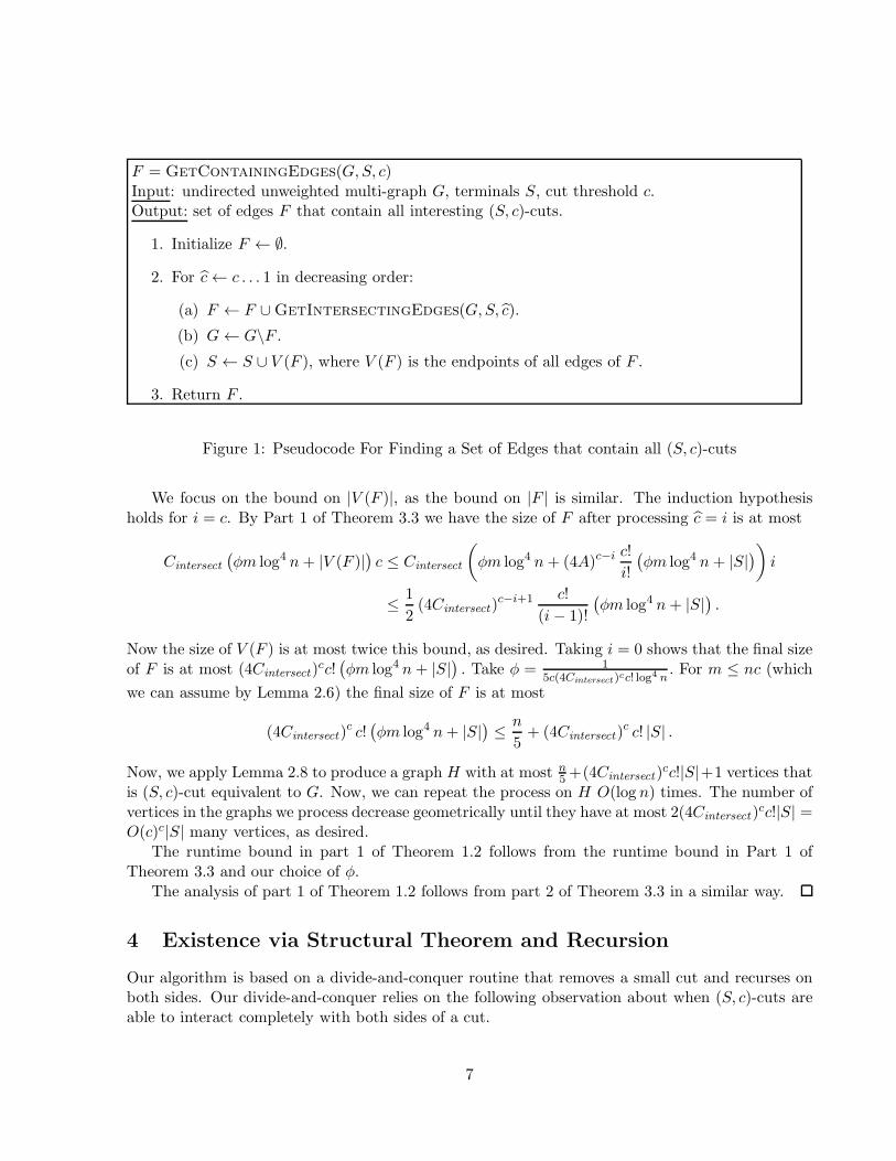
F = GetContainingEdges(G,S, c)Input: undirected unweighted multi-graph G, terminals S, cut threshold c.Output: set of edges F that contain all interesting (S, c)-cuts.
1. Initialize F ← ∅.
2. For c← c . . . 1 in decreasing order:
(a) F ← F ∪GetIntersectingEdges(G,S, c).
(b) G← G\F .
(c) S ← S ∪ V (F ), where V (F ) is the endpoints of all edges of F .
3. Return F .
Figure 1: Pseudocode For Finding a Set of Edges that contain all (S, c)-cuts
We focus on the bound on |V (F )|, as the bound on |F | is similar. The induction hypothesisholds for i = c. By Part 1 of Theorem 3.3 we have the size of F after processing c = i is at most
Cintersect
(φm log4 n+ |V (F )|
)c ≤ Cintersect
(φm log4 n+ (4A)c−i c!
i!
(φm log4 n+ |S|
))i
≤ 1
2(4Cintersect)
c−i+1 c!
(i− 1)!
(φm log4 n+ |S|
).
Now the size of V (F ) is at most twice this bound, as desired. Taking i = 0 shows that the final sizeof F is at most (4Cintersect)
cc!(φm log4 n+ |S|
). Take φ = 1
5c(4Cintersect )cc! log4 n
. For m ≤ nc (which
we can assume by Lemma 2.6) the final size of F is at most
(4Cintersect)c c!
(φm log4 n+ |S|
)≤ n
5+ (4Cintersect)
c c! |S| .
Now, we apply Lemma 2.8 to produce a graph H with at most n5 +(4Cintersect)
cc!|S|+1 vertices thatis (S, c)-cut equivalent to G. Now, we can repeat the process on H O(log n) times. The number ofvertices in the graphs we process decrease geometrically until they have at most 2(4Cintersect )
cc!|S| =O(c)c|S| many vertices, as desired.
The runtime bound in part 1 of Theorem 1.2 follows from the runtime bound in Part 1 ofTheorem 3.3 and our choice of φ.
The analysis of part 1 of Theorem 1.2 follows from part 2 of Theorem 3.3 in a similar way.
4 Existence via Structural Theorem and Recursion
Our algorithm is based on a divide-and-conquer routine that removes a small cut and recurses onboth sides. Our divide-and-conquer relies on the following observation about when (S, c)-cuts areable to interact completely with both sides of a cut.
7
Lemma 4.1. Let F be a cut given by the partition V = V1 ·∪V2 in G = (V,E) such that both G[V1]and G[V2] are connected, and S1 = V1 ∩ S and S2 = V2 ∩ S be the partition of S induced by thiscut. If F1 intersects all (S1 ∪v2, c)-terminal cuts in G/V2, the graph formed by contracting all ofV2 into a single vertex v2, and similarly F2 intersects all (S2 ∪v1, c)-terminal cuts in G/V1, thenF1 ∪ F2 ∪ F intersects all (S, c)-cuts in G as well.
Proof. Consider some cut F of size at most c.If F uses an edge from F , then it has at most c − 1 edges in G\F , and thus in any connected
component as well.If F has at most c − 1 edges in G[V1], then because removing F already disconnected V1 and
V2, and removing F1 can only further disconnect things, no connected component in V1 can have cor more edges.
So the only remaining case is if F is entirely contained on one of the sides. Without loss ofgenerality assume F is entirely contained in V1, i.e. F ⊆ E(G[V1]). Because no edges from G[V2]are removed and G[V2] is connected, all of S2 must be on one side of the cut, and can therefore berepresented by a single vertex v2.
So using the induction hypothesis on the cut F in G/V2 with the terminal separation given byall of S2 replaced by v2 gives that F has at most c− 1 edges in any connected component of
(G/V2) \F1.
Because connected components are unchanged under contracting connected subsets, we get that Fhas at most c− 1 edges in any connected components of G\F1 as well.
However, for such a partition to make progress, we also need at least two terminals to becomecontracted together when V1 or V2 are contracted. Building this into the definition leads to our keydefinition of a non-trivial S-separating cut:
Definition 4.2. A non-trivial S-separating cut is a separation of V into V1 ·∪ V2 such that:
1. the induced subgraphs on V1 and V2, G[V1] and G[V2] are both connected.
2. |V1 ∩ S| ≥ 2, |V2 ∩ S| ≥ 2.
Such cuts are critical for partitioning and recursing on the two resulting pieces. Connectivity ofG[V1] and G[V2] is necessary for applying Lemma 4.1, and |V1 ∩ S| ≥ 2, |V2 ∩ S| ≥ 2 are necessaryto ensure that making this cut and recursing makes progress.
We now study the set of graphs G and terminals S for which a nontrivial cut exists. Forexample, consider for example when G is a star graph (a single vertex with n− 1 vertex connectedto it) and all vertices are terminals. In this graph, the side of the cut not containing the center canonly have a single vertex, hence there are no nontrivial cuts.
We can, in fact, prove the converse: if no such interesting separations exist, we can terminateby only considering the |S| separations of S formed with one terminal on one of the sides. Wedefine these cuts to be the s-isolating cuts.
Definition 4.3. For a graph G with terminal set S and some s ∈ S, a s-isolating cut is a split ofthe vertices V = VA ·∪ VB such that s is the only terminal in VA, i.e. s ∈ VA, (S\u) ⊆ VB .
8
Lemma 4.4. If S is a subset of at least 4 terminals in an undirected graph G such that there doesnot exist a non-trivial S separating cut of size at most c, then
F =⋃
s∈S|Mincut(G,s,S\s)|≤c
Mincut (G, s , S\ s)
contains all (S, c) cuts of G. Here, F is the union of all s-isolating cuts of size at most c.
Proof. Consider a graph with no non-trivial S separating cut of size at most c, but there is apartition of S, S = S1 ·∪S2, such that the minimum cut between S1 and S2, V1 and V2, has at mostc edges, and |S1|, |S2| ≥ 2.
Let E be one such cut, and consider the graph
G = G/(E\E
),
that is, we contract all edges except the ones on this cut. Note that G has at least 2 vertices.Consider a spanning tree T of G. By minimality of E, each node of T must contain at least one
terminal. Otherwise, we can keep one edge from such a node without affecting the distribution ofterminal vertices.
We now show that no vertex of T can contain |S| − 1 terminals. If T has exactly two vertices,then one vertex must correspond to S1 and one must correspond to S2, so no vertex has |S| − 1terminals. If T has at least 3 vertices, then because every vertex contains at least one terminal, novertex in T can contain |S| − 1 vertices.
Also, each leaf of T can contain at most one terminal, otherwise deleting the edge adjacent tothat leaf forms a nontrivial cut.
Now consider any non-leaf node of the tree, r. As r is a non-leaf node, at it has at least twodifferent neighbors that lead to leaf vertices.
Reroot this tree at r, and consider some neighbor of r, x. If the subtree rooted at x has morethan 2 terminals, then cutting the rx edge results in two components, each containing at least twoterminals (the component including r has at least one other neighbor that contains a terminal).Thus, the subtree rooted at x can contain at most one terminal, and must therefore be a singletonleaf.
Hence, the only possible structure of T is a star centered at r (which may contain multipleterminals), and each leaf having a exactly one terminal in it. This in turn implies that G also mustbe a star, i.e. G has the same edges as T but possibly with multi-edges. This is because any edgebetween two leaves of a star forms a connected cut by disconnecting those vertices from r.
By minimality, each cut separating the root from leaf is a minimal cut for that single terminal,and these cuts are disjoint. Thus taking the union of edges of all these singleton cuts gives a cutthat splits S the same way, and has the same size.
Note that Lemma 4.4 is not claiming all the (S, c)-cuts of S are singletons. Instead, it says thatany (S, c)-cut can be formed from a union of single terminal cuts.
Combining Lemma 4.1 and 4.4, we obtain the recursive algorithm in Figure 2, which demon-strates the existence of O(|S| · c) sized (S, c)-cut-intersecting subsets. If there is a nontrivial S-separating cut, the algorithm in Line 3 finds it and recurses on both sides of the cut using Lemma4.1. Otherwise, by Lemma 4.4, the union of the s-isolating cuts of size at most c contains all(S, c)-cuts, so the algorithm keeps the edges of those cuts in Line 4a.
9
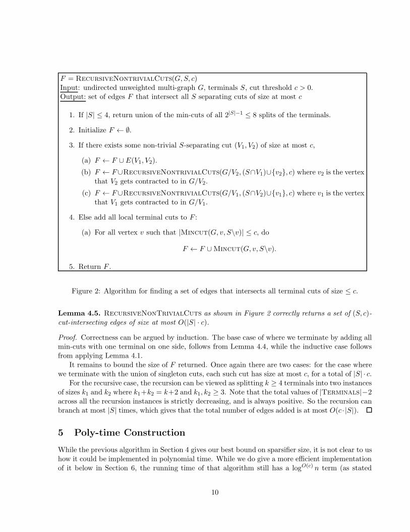
F = RecursiveNontrivialCuts(G,S, c)Input: undirected unweighted multi-graph G, terminals S, cut threshold c > 0.Output: set of edges F that intersect all S separating cuts of size at most c
1. If |S| ≤ 4, return union of the min-cuts of all 2|S|−1 ≤ 8 splits of the terminals.
2. Initialize F ← ∅.
3. If there exists some non-trivial S-separating cut (V1, V2) of size at most c,
(a) F ← F ∪ E(V1, V2).
(b) F ← F∪RecursiveNontrivialCuts(G/V2, (S∩V1)∪v2, c) where v2 is the vertexthat V2 gets contracted to in G/V2.
(c) F ← F∪RecursiveNontrivialCuts(G/V1, (S∩V2)∪v1, c) where v1 is the vertexthat V1 gets contracted to in G/V1.
4. Else add all local terminal cuts to F :
(a) For all vertex v such that |Mincut(G, v, S\v)| ≤ c, do
F ← F ∪Mincut(G, v, S\v).
5. Return F .
Figure 2: Algorithm for finding a set of edges that intersects all terminal cuts of size ≤ c.
Lemma 4.5. RecursiveNonTrivialCuts as shown in Figure 2 correctly returns a set of (S, c)-cut-intersecting edges of size at most O(|S| · c).
Proof. Correctness can be argued by induction. The base case of where we terminate by adding allmin-cuts with one terminal on one side, follows from Lemma 4.4, while the inductive case followsfrom applying Lemma 4.1.
It remains to bound the size of F returned. Once again there are two cases: for the case wherewe terminate with the union of singleton cuts, each such cut has size at most c, for a total of |S| · c.
For the recursive case, the recursion can be viewed as splitting k ≥ 4 terminals into two instancesof sizes k1 and k2 where k1+k2 = k+2 and k1, k2 ≥ 3. Note that the total values of |Terminals|−2across all the recursion instances is strictly decreasing, and is always positive. So the recursion canbranch at most |S| times, which gives that the total number of edges added is at most O(c · |S|).
5 Poly-time Construction
While the previous algorithm in Section 4 gives our best bound on sparsifier size, it is not clear to ushow it could be implemented in polynomial time. While we do give a more efficient implementationof it below in Section 6, the running time of that algorithm still has a logO(c) n term (as stated
10
in Theorem 1.2 Part 1). In this section, we give a more efficient algorithm that returns sparsifiersof larger size, but ultimately leads to the faster running time given in Theorem 1.2 Part 2. Itwas derived by working backwards from the termination condition of taking all the cuts with oneterminal on one side in Lemma 4.4.
Recall that a Steiner cut is a cut with at least one terminal one both sides. The algorithmhas the same high level recursive structure, but it instead only finds the minimum Steiner cut orcertifies that its size is greater than c. This takes O(m+nc3) time using an algorithm by Cole andHariharan [CH03].
It is direct to check that both sides of a minimum Steiner cut are connected. This is importanttowards our goal of finding a non-trivial S-separating cut, defined in Definition 4.2.
Lemma 5.1. If (VA, VB) is the global minimum S-separating cut in a connceted graph G, then bothG[VA] and G[VB ] must be connected.
Proof. Suppose for the sake of contradiction that VA is disconnected. That is, VA = VA1 ·∪ VA2,there are no edges between VA1 and VA2.
Without loss of generality assume VA1 contains a terminal. Also, VB contains at least oneterminal because (VA, VB) is S-separating.
Then because G is connected, there is an edge between VA1 and VB. Then the cut (VA1, VA2∪VB)has strictly fewer edges crossing, and also terminals on both sides, a contradiction to (VA, VB) beingthe minimum S separating cut.
So the only bad case that prevents us from recursing is the case where the minimum Steinercut has a single terminal s on some side. That is, one of the s-isolating cuts from Definition 4.3 isalso a minimum Steiner cut.
We can handle this case through an extension of Lemma 4.1. Specifically, we show that for acut with both sides connected, we can contract a side of the cut along with the cut edges beforerecursing.
Lemma 5.2. Let F be a cut given by the partition V = V1 ·∪V2 in G = (V,E) such that both G[V1]and G[V2] are connected, and S1 = V1∩S and S2 = V2∩S be the partition of S induced by this cut.If F1 intersects all (S1 ∪ v2, c)-terminal cuts in G/V2/F , the graph formed by contracting all ofV2 and all edges in F into a single vertex v2, and similarly F2 intersects all (S2 ∪ v1, c)-terminalcuts in G/V1/F , then F1 ∪ F2 ∪ F intersects all (S, c)-cuts in G as well.
Proof. Consider some cut F of size at most c.If F uses an edge from F , then it has at most c − 1 edges in G\F , and thus in any connected
component as well.If F has at most c − 1 edges in G[V1], then because removing F already disconnected V1 and
V2, and removing F1 can only further disconnect things, no connected component in V1 can have cor more edges.
The only remaining case is if F is entirely contained on one of the sides. Without loss ofgenerality assume F is entirely contained in V1, i.e. F ⊆ E(G[V1]). Because no edges from G[V2]and F are removed and G[V2] is connected, all edges in G[V2] and F must not be cut and hencecan be contracted into a single vertex v2.
11
So using the induction hypothesis on the cut F in G/V2/F with the terminal separation givenby all of S2 replaced by v2 gives that F has at most c− 1 edges in any connected component of
(G/V2/F ) \F1.
Because connected components are unchanged under contracting connected subsets, we get that Fhas at most c− 1 edges in any connected components of G\F1 as well.
Now, a natural way to handle the case where a minimum Steiner cut has a single terminal s onsome side is to use Lemma 5.2 to contract across the cut to make progress. However, it may bethe case that for some s ∈ S, there are are many minimum s-isolating cuts: consider for examplethe length n path with only the endpoints as terminals. If we always pick the edge closest to s asthe minimum s-isolating cut, we may have to continue n rounds, and thus add all n edges to ourset of intersecting edges.
To remedy this, we instead pick a “maximal” s-isolating minimum cut. One way to find amaximal s-isolating cut is to repeatedly contract across an s-isolating minimum cut using Lemma5.2 until its size increases. At that point, we add the last set of edges found in the cut to the set ofintersecting edges. We have made progress because the value of the minimum s-isolating cut in thecontracted graph must have increased by at least 1. While there are many ways to find a maximals-isolating minimum cut, the way described here extends to our analysis in Section 6.2.
Pseudocode of this algorithm is shown in Figure 3, and the procedure for the repeated contrac-tions to find a maximal s-isolating cut described in the above paragraph is in Line 3d.
Discussion of algorithm in Figure 3. We clarify some lines in the algorithm of Figure 3. Ifthe algorithm finds a nontrivial S-separating cut as the Steiner minimum cut, it returns the resultof the recursion in Line 3(c)i, and does not execute any of the later lines in the algorithm. InLine 3(d)ii, in addition to checking that the s-isolating minimum cut size is still x, we also mustcheck that s does not get contracted with another terminal. Otherwise, contracting across that cutmakes global progress by reducing the number of terminals by 1. In Line 3(d)iiC, note that wecan still view s as a terminal in G← G/V1/F , as we have assumed that this contraction does notmerge s with any other terminals.
Lemma 5.3. For any graph G, terminals S, and cut value c, Algorithm RecursiveSteinerCuts
as shown in Figure 3 runs in O(n2c4) time and returns a set at most O(|S|c2) edges that intersectall (S, c)-cuts.
Proof. We assume m ≤ nc throughout, as we can reduce to this case in O(mc) time by Lemma 2.6.Note that the recursion in Line 3(c)i can only branch O(|S|) times, by the analysis in Lemma
4.5. Similarly, the case where s gets contracted with another terminal in Line 3(d)ii can only occurO(|S|) times.
Therefore, we only create O(|S|) distinct terminals throughout the algorithm. Let s be aterminal created at some point during the algorithm. By monotonicity of cuts in Lemma 2.1, theminimum s-isolating cut can only increase in size c times, hence F is the union of O(|S|c) cuts ofsize at most c. Therefore, F has at most O(|S|c2) edges.
To bound the runtime, we use the total number of edges in the graphs in our recursive algorithmas a potential function. This potential function starts at m. Note that the recursion of Line 3(c)i
12
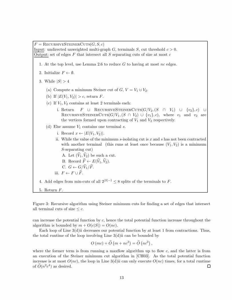
F = RecursiveSteinerCuts(G,S, c)Input: undirected unweighted multi-graph G, terminals S, cut threshold c > 0.Output: set of edges F that intersect all S separating cuts of size at most c
1. At the top level, use Lemma 2.6 to reduce G to having at most nc edges.
2. Initialize F ← ∅.
3. While |S| > 4
(a) Compute a minimum Steiner cut of G, V = V1 ·∪ V2.
(b) If |E(V1, V2)| > c, return F .
(c) If V1, V2 contains at least 2 terminals each:
i. Return F ∪ RecursiveSteinerCuts(G/V2, (S ∩ V1) ∪ v2, c) ∪RecursiveSteinerCuts(G/V1, (S ∩ V2) ∪ v1, c), where v1 and v2 arethe vertices formed upon contracting of V1 and V2 respectively.
(d) Else assume V1 contains one terminal s.
i. Record x← |E(V1, V2)|.ii. While the value of the minimum s-isolating cut is x and s has not been contracted
with another terminal (this runs at least once because (V1, V2) is a minimumS-separating cut)
A. Let (V1, V2) be such a cut.
B. Record F ← E(V1, V2).
C. G← G/V1/F .
iii. F ← F ∪ F .
4. Add edges from min-cuts of all 2|S|−1 ≤ 8 splits of the terminals to F .
5. Return F .
Figure 3: Recursive algorithm using Steiner minimum cuts for finding a set of edges that intersectall terminal cuts of size ≤ c.
can increase the potential function by c, hence the total potential function increase throughout thealgorithm is bounded by m+O(c|S|) = O(nc).
Each loop of Line 3(d)ii decreases our potential function by at least 1 from contractions. Thus,the total runtime of the loop involving Line 3(d)ii can be bounded by
O (mc) + O(m+ nc3
)= O
(nc3
),
where the former term is from running a maxflow algorithm up to flow c, and the latter is froman execution of the Steiner minimum cut algorithm in [CH03]. As the total potential functionincrease is at most O(nc), the loop in Line 3(d)ii can only execute O(nc) times, for a total runtimeof O(n2c4) as desired.
13
Our further speedup of this routine in Section 6 also uses a faster variant of RecursiveStein-
erCuts as base case, which happens when |S| is too small. Here the main observation is thatA modification to Algorithm as shown in Figure 3 can reduce the runtime.
Lemma 5.4. For any graph G, terminals S, and cut value c, there is an algorithm that runs inO(mc+ n|S|c4) time and returns a set at most O(|S|c2) edges that intersect all (S, c)-cuts.
Proof. We modify RecursiveSteinerCuts as shown in Figure 3 and its analysis as given inLemma 5.3 above. Specifically, we modify how we compute a maximal s-isolating minimum cut inLine 3(d)ii. For any partition S = S1 ·∪ S2, by submodularity of cuts it is known that there is aunique maximal subset V1 ⊆ V such that
S1 ⊆ V1,
S2 ⊆ V \V1,
|E (V1, V2)| = |Mincut (G,S1, S2)| .
Also, this maximal set can be computed in O(mc) time by running the Ford-Fulkerson augmentingpath algorithm, with S2 as source, and S1 as sink. The connectivity value of c means at most caugmenting paths need to be found, and the set V2 can be set to the vertices that can still reachthe sink set S2 in the residual graph [FH75]. Now set V1 = V \V2. Thus by setting S1 ← s, wecan use the corresponding computed set V1 as the representative of the maximal s-isolating Steinerminimum cut.
Now we analyze the runtime of this procedure. First, in we reduce the number of edges toat most nc in O(mc) time. As in the proof of Lemma 5.3, all graphs in the recursion have atmost O(nc) edges. The recursion in Line 3(c)i can only branch |S| times, and we only need tocompute O(c|S|) maximal s-isolating Steiner minimum cuts throughout the algorithm. Each callto the Cole-Hariharan algorithm [CH03] requires O(m+nc3) = O(nc3) time, for a total runtime ofO(nc3 · c|S|) = O(n|S|c4) as desired.
6 Nearly-Linear Time Constructions Using Expanders
In this section We now turn our attention to efficiently finding these vertex sparsifiers. Here weutilize insights from recent results on finding c-vertex cuts [NSY19a, NSY19b, FY19], namely thatin a well connected graph, any cut of size at most c must have a very small side. This notion ofconnectivity is formalized through the notion of graph conductance.
Definition 6.1. In an undirected unweighted graph G = (V,E), denote the volume of a subset ofvertices, vol(S), as the total degrees of its vertices. The conductance of a cut S is then
ΦG (S) =|∂ (S)|
min vol (S) , vol (V \S) ,
and the conductance of a graph G = (V,E) is the minimum conductance of a subset of vertices:
Φ (G) = minS⊆V
ΦG (S) .
14
The ability to remove edges and add terminals means we can use expander decomposition toreduce to the case where the graph has high conductance. Here we utilize expander decompositions,as stated by Saranurak and Wang [SW19]:
Lemma 6.2. (Theorem 1.2. of [SW19], Version 2 https:// arxiv.org/pdf/ 1812. 08958v2.pdf )There exists an algorithm ExpanderDecompose that for any undirected unweighted graph G andany parameter φ, decomposes in O(m log4 nφ−1) time G into pieces of conductance at least φ sothat at most O(mφ log3 n) edges are between the pieces.
Note that if a graph has conductance φ, any cut of size at most c must have
min vol (S) , vol (V \S) ≤ cφ−1. (1)
Algorithmically, we can further leverage it in two ways, both of which are directly motivatedby recent works on vertex connectivity [NSY19a, FY19, NSY19b].
6.1 Enumeration of All Small Cuts by their Smaller Sides
In a graph with expansion φ, we can enumerate all cuts of size at most c in time exponential in cand φ.
Lemma 6.3. In a graph G with conductance φ we can enumerate all cuts of size at most c withconnected smaller side in time O(n · (cφ−1)2c).
Proof. We first enumerate over all starting vertices. For a starting vertex u, we repeatedly performthe following process.
1. perform a DFS from u until it reaches more than cφ−1 vertices.
2. Pick one of the edges among the reached vertices as a cut edge.
3. Remove that edge, and recursively start another DFS starting at u.
After we have done this process at most c times, we check whether the edges form a valid cut, andstore it if so.
By Equation 1, the smaller side of the can involve at most cφ−1 vertices. Consider such a cutwith S as the smaller side, F = E(S, V \ S), and |S| ≤ cφ−1. Then if we picked some vertexu ∈ S as the starting point, the DFS tree rooted at u must contain some edge in F at some point.Performing an induction with this edge removed then gives that the DFS starting from u will findthis cut.
Because there can be at most O((cφ−1)2) different edges picked among the vertices reached, thetotal work performed in the c layers of recursion is O((cφ−1)2c).
Furthermore, it suffices to enumerate all such cuts once at the start, and reuse them as weperform contractions.
Lemma 6.4. If F is a set of edges that form a cut in G/E, that is, G with a subset of edges Econtracted, then F is also a cut in G.
Note that this lemma also implies that an expander stays so under contractions. So we do noteven need to re-partition the graph as we recurse.
15
Proof of Theorem 3.3 Part 1. First, we perform expander decomposition, remove the inter-clusteredges, and add their endpoints as terminals.
Now, we describe the modifications to GetIntersectingEdgesSlow that makes it efficient.Lemma 2.3, and Lemma 2.5 allows us to consider the pieces separately.Now at the start of each recursive call, enumerate all cuts of size at most c, and store the
vertices on the smaller side, which by Equation 1 above has size at most O(cφ−1). When such a cutis found, we only invoke recursion on the smaller side (in terms of volume). For the larger piece,we can continue using the original set of cuts found during the search.
To use a cut from a pre-contracted state, we need to:
1. check if all of its edges remain (using a union-find data structure).
2. check if both portions of the graph remain connected upon removal of this cut – this can bedone by explicitly checking the smaller side, and certifying the bigger side using a dynamicconnectivity data structure by removing all edges from the smaller side.
Since we contract each edge at most once, the total work done over all the larger side is at most
O(m (cφ)−2c
),
where we have included the logarithmic factors from using the dynamic connectivity data structure.Furthermore, the fact that we only recurse on things with half as many edges ensures that eachedge participates in the cut enumeration process at most O(log n) times. Combining these thengives the overall running time.
6.2 Using Local Cut Algorithms
A more recent development are local cut algorithms, which for a vertex v can whether there is acut of size at most c such that the side with v has volume at most ν. The runtime is linear in cand ν.
Theorem 6.5 (Theorem 3.1 of [NSY19b]). Let G be a graph and let v ∈ V (G) be a vertex. For aconnectivity parameter c and volume parameter ν, there is an algorithm that with high probabilityeither
1. Certifies that there is no cut of size at most c such that the side with v has volume at most ν.
2. Returns a cut of size at most c such that the side with v has volume at most 130cν. It runsin time O(c2ν).
Let v be a vertex. We now formalize the notion of the smallest cut that is local around v.
Definition 6.6 (Local cuts). For a vertex v ∈ G define LocalCut(v) to be
minV=V1 ·∪V2
v∈V1
vol(V1)≤vol(V2)
|E(V1, V2)|.
We now combine Theorem 6.5 with the observation from Equation 1 in order to control thevolume of the smaller side of the cut in an expander.
16
Lemma 6.7. Let G be a graph with conductance at most φ, and let S be a set of terminals. If|S| ≥ 500c2φ−1 then for any vertex s ∈ S we can with high probability in O(c3φ−1) time eithercompute LocalCut(s) or certify that LocalCut(s) > c.
Proof. We binary search on the size of the minimum Steiner cut with s on the smaller side, andapply Theorem 6.5. The smaller side of a Steiner cut has volume at most cφ−1. Therefore, if|S| ≥ 500c2φ−1 then the cut returned by Theorem 6.5 for ν = cφ−1 will always be a Steiner cut, as130νc ≤ |S|/2. The runtime is O(νc2) = O(c3φ−1) as desired.
We can substitute this faster cut-finding procedure into RecursiveSteinerCuts to get thefaster running time stated in Theorem 3.3 Part 2.
Proof of Theorem 3.3 Part 2. First, we perform expander decomposition, remove the inter-clusteredges, and add their endpoints as terminals.
Now, we describe the modifications we need to make to Algorithm RecursiveSteinerCuts
as shown in Figure 3. First, we terminate if |S| ≤ 500c2φ−1 and use the result of Lemma 5.4.Otherwise, instead of using the Cole-Hariharan algorithm, we compute the terminal s ∈ S withminimal value of LocalCut(s). This gives us a Steiner minimum cut. If the corresponding cut isa nontrivial S-separating cut then we recurse as in Line 3(c)i. Otherwise, we perform the loop inLine 3(d)ii.
We now give implementation details for computing the terminal s ∈ S with minimal value ofLocalCut(s). By Lemma 2.1 we can see that for a terminal s, LocalCut(s) is monotone throughoutthe algorithm. For each terminal s, our algorithm records the previous value of LocalCut(s) com-puted. Because this value is monotone, we need only check vertices s whose value of LocalCut(s)could still possibly be minimal. Now, either LocalCut(s) is certified to be minimal among all s,or the value of LocalCut(s) is higher than the previously recorded value. Note that this can onlyoccur O(c|S|) times, as we stop processing a vertex s if LocalCut(s) > c.
We now analyze the runtime. We first bound the runtime from the cases |S| ≤ 500c2φ−1. Thetotal number of vertices and edges in the leaves of the recursion tree is at most O(mc). Therefore,by Lemma 5.4, the total runtime from these is at most
O(500c2φ−1 ·mc · c4) = O(mφ−1c7).
Now, the loop of Line 3(d)ii can only execute cφ−1 times, because the volume of any s-isolatingcut has size at most cφ−1. Each iteration of the loop requires O(c3φ−1) time by Lemma 6.7.Therefore, the total runtime of executing the loop and calls to it is bounded by
O(c|S| · cφ−1 · c3φ−1
)= O(|S|φ−2c6).
Combining these shows Theorem 3.3 Part 2.
Acknowledgements
We thank Gramoz Goranci, Jakub Lacki, Thatchaphol Saranurak, and Xiaorui Sun for multipleenlightening discussions on this topic. In particular, the graph partitioning based efficient construc-tions in Section 6 are directly motivated by conversations with Xiaorui. We also thank ParaniyaChamelsook, Syamantak Das, Bundit Laekhanukit, Antonio Molina, Bryce Sandlund, and DanielVaz for communicating with us about unpublished related results.
17
References
[ADK+16] I. Abraham, D. Durfee, I. Koutis, S. Krinninger, and R. Peng. On fully dynamic graphsparsifiers. In 2016 IEEE 57th Annual Symposium on Foundations of Computer Science(FOCS), pages 335–344, Oct 2016.
[AKLT15] Sepehr Assadi, Sanjeev Khanna, Yang Li, and Val Tannen. Dynamic sketching for graphoptimization problems with applications to cut-preserving sketches. In FSTTCS, 2015.Available at https://arxiv.org/abs/1510.03252.
[CH03] Richard Cole and Ramesh Hariharan. A fast algorithm for computing steiner edge con-nectivity. In Proceedings of the 35th Annual ACM Symposium on Theory of Computing,June 9-11, 2003, San Diego, CA, USA, pages 167–176, 2003.
[CLLM10] Moses Charikar, Tom Leighton, Shi Li, and Ankur Moitra. Vertex sparsifiers andabstract rounding algorithms. In 51th Annual IEEE Symposium on Foundations ofComputer Science, FOCS 2010, October 23-26, 2010, Las Vegas, Nevada, USA, pages265–274, 2010.
[DGGP19] David Durfee, Yu Gao, Gramoz Goranci, and Richard Peng. Fully dynamic spectralvertex sparsifiers and applications. In Proceedings of the 51st Annual ACM SIGACTSymposium on Theory of Computing, STOC 2019, Phoenix, AZ, USA, June 23-26,2019., pages 914–925, 2019. Available at: https://arxiv.org/abs/1906.10530.
[DKP+17] David Durfee, Rasmus Kyng, John Peebles, Anup B Rao, and Sushant Sachdeva. Sam-pling random spanning trees faster than matrix multiplication. In Proceedings of the49th Annual ACM SIGACT Symposium on Theory of Computing, pages 730–742. ACM,2017. Available at: https://arxiv.org/abs/1611.07451.
[DV94] Yefim Dinitz and Alek Vainshtein. The connectivity carcass of a vertex subset in agraph and its incremental maintenance. In Proceedings of the twenty-sixth annual ACMsymposium on Theory of computing, pages 716–725. ACM, 1994.
[DV95] Ye. Dinitz and A. Vainshtein. Locally orientable graphs, cell structures, and a newalgorithm for the incremental maintenance of connectivity carcasses. In Proceedingsof the Sixth Annual ACM-SIAM Symposium on Discrete Algorithms, SODA ’95, pages302–311, 1995.
[DW98] Yefim Dinitz and Jeffery R. Westbrook. Maintaining the classes of 4-edge-connectivityin a graph on-line. Algorithmica, 20(3):242–276, 1998.
[EGK+14] Matthias Englert, Anupam Gupta, Robert Krauthgamer, Harald Racke, Inbal Talgam-Cohen, and Kunal Talwar. Vertex sparsifiers: New results from old techniques. SIAMJ. Comput., 43(4):1239–1262, 2014.
[Epp94] David Eppstein. Offline algorithms for dynamic minimum spanning tree problems. J.Algorithms, 17(2):237–250, September 1994.
[FH75] Delbert Ray Fulkerson and Gary Harding. On edge-disjoint branchings. Technicalreport, CORNELL UNIV ITHACA NY DEPT OF OPERATIONS RESEARCH, 1975.
18
[FHKQ16] Stefan Fafianie, Eva-Maria C. Hols, Stefan Kratsch, and Vuong Anh Quyen. Pre-processing under uncertainty: Matroid intersection. In 41st International Sym-posium on Mathematical Foundations of Computer Science, MFCS 2016, Au-gust 22-26, 2016 - Krakow, Poland, pages 35:1–35:14, 2016. Available athttps://core.ac.uk/download/pdf/62922404.pdf.
[FKQ16] Stefan Fafianie, Stefan Kratsch, and Vuong Anh Quyen. Preprocessing under uncer-tainty. In 33rd Symposium on Theoretical Aspects of Computer Science (STACS 2016),volume 47, pages 33:1–33:13, 2016.
[FY19] Sebastian Forster and Liu Yang. A faster local algorithm for detecting bounded-sizecuts with applications to higher-connectivity problems. CoRR, abs/1904.08382, 2019.
[GHP17a] Gramoz Goranci, Monika Henzinger, and Pan Peng. Improved guarantees for vertexsparsification in planar graphs. In 25th Annual European Symposium on Algorithms,ESA 2017, September 4-6, 2017, Vienna, Austria, pages 44:1–44:14, 2017. Availableat: https://arxiv.org/abs/1702.01136.
[GHP17b] Gramoz Goranci, Monika Henzinger, and Pan Peng. The power of vertex sparsifiersin dynamic graph algorithms. In 25th Annual European Symposium on Algorithms,ESA 2017, September 4-6, 2017, Vienna, Austria, pages 45:1–45:14, 2017. Availableat: https://arxiv.org/abs/1712.06473.
[GHP18] Gramoz Goranci, Monika Henzinger, and Pan Peng. Dynamic effective resistances andapproximate schur complement on separable graphs. In 26th Annual European Sym-posium on Algorithms, ESA 2018, August 20-22, 2018, Helsinki, Finland, pages 40:1–40:15, 2018. Available at: https://arxiv.org/abs/1802.09111.
[GI91] Zvi Galil and Giuseppe F Italiano. Fully dynamic algorithms for edge connectivityproblems. In Proceedings of the twenty-third annual ACM symposium on Theory ofcomputing, pages 317–327. ACM, 1991.
[GR16] Gramoz Goranci and Harald Racke. Vertex sparsification in trees. In Approximationand Online Algorithms - 14th International Workshop, WAOA 2016, Aarhus, Den-mark, August 25-26, 2016, Revised Selected Papers, pages 103–115, 2016. Available at:https://arxiv.org/abs/1612.03017.
[HdLT98] Jacob Holm, Kristian de Lichtenberg, and Mikkel Thorup. Poly-logarithmic determin-istic fully-dynamic algorithms for connectivity, minimum spanning tree, 2-edge, andbiconnectivity. In Proceedings of the thirtieth annual ACM symposium on Theory ofcomputing, STOC ’98, pages 79–89, New York, NY, USA, 1998. ACM.
[KL15] Adam Karczmarz and Jakub Lacki. Fast and simple connectivity in graph timelines.In Frank Dehne, Jorg-Rudiger Sack, and Ulrike Stege, editors, Algorithms and DataStructures: 14th International Symposium, WADS 2015, pages 458–469, 2015.
[KLP+16] Rasmus Kyng, Yin Tat Lee, Richard Peng, Sushant Sachdeva, and Daniel A Spielman.Sparsified cholesky and multigrid solvers for connection laplacians. In Proceedings of
19
the 48th Annual ACM SIGACT Symposium on Theory of Computing, pages 842–850.ACM, 2016. Available at http://arxiv.org/abs/1512.01892.
[Kop12] Sergey Kopeliovich. Offline solution of connectivity and 2-edge-connectivity problems for fully dynamic graphs, 2012. Available athttp://se.math.spbu.ru/SE/diploma/2012/s/Kopeliovich_diploma.pdf.
[KR17] Robert Krauthgamer and Inbal Rika. Refined vertex sparsifiers of planar graphs. CoRR,abs/1702.05951, 2017.
[KS16] Rasmus Kyng and Sushant Sachdeva. Approximate gaussian elimination for laplacians -fast, sparse, and simple. In IEEE 57th Annual Symposium on Foundations of ComputerScience, FOCS 2016, 9-11 October 2016, Hyatt Regency, New Brunswick, New Jersey,USA, pages 573–582, 2016. Available at http://arxiv.org/abs/1605.02353.
[KW12] Stefan Kratsch and Magnus Wahlstrom. Representative sets and irrelevant vertices:New tools for kernelization. In Proceedings of the 2012 IEEE 53rd Annual Symposiumon Foundations of Computer Science, FOCS ’12, pages 450–459, 2012. Available athttps://arxiv.org/abs/1111.2195.
[LS13] Jackub Lacki and Piotr Sankowski. Reachability in graph timelines. ITCS, 2013.
[MM10] Konstantin Makarychev and Yury Makarychev. Metric extension operators, vertexsparsifiers and lipschitz extendability. In 51th Annual IEEE Symposium on Foundationsof Computer Science, FOCS 2010, October 23-26, 2010, Las Vegas, Nevada, USA, pages255–264, 2010.
[MS18] Antonio Molina and Bryce Sandlund. Historical optimization with applications to dy-namic higher edge connectivity. 2018.
[NI92] Hiroshi Nagamochi and Toshihide Ibaraki. A linear-time algorithm for finding a sparsek-connected spanning subgraph of ak-connected graph. Algorithmica, 7(1-6):583–596,1992.
[NSY19a] Danupon Nanongkai, Thatchaphol Saranurak, and Sorrachai Yingchareonthawornchai.Breaking quadratic time for small vertex connectivity and an approximation scheme.In Proceedings of the 51st Annual ACM SIGACT Symposium on Theory of Computing,STOC 2019, Phoenix, AZ, USA, June 23-26, 2019., pages 241–252, 2019. Available at:https://arxiv.org/abs/1904.04453.
[NSY19b] Danupon Nanongkai, Thatchaphol Saranurak, and Sorrachai Yingchareonthawornchai.Computing and testing small vertex connectivity in near-linear time and queries. CoRR,abs/1905.05329, 2019. Available at : http://arxiv.org/abs/1905.05329.
[PSS19] Richard Peng, Bryce Sandlund, and Daniel Dominic Sleator. Optimal offline dynamic2, 3-edge/vertex connectivity. In Algorithms and Data Structures - 16th InternationalSymposium, WADS 2019, Edmonton, AB, Canada, August 5-7, 2019, Proceedings,pages 553–565, 2019. Available at: https://arxiv.org/abs/1708.03812.
20
[SW19] Thatchaphol Saranurak and Di Wang. Expander decomposition and pruning: Faster,stronger, and simpler. In SODA, pages 2616–2635. SIAM, 2019. Available at:https://arxiv.org/abs/1812.08958.
21