high-power ion thruster technology

I • I

t 1

!

NASA Contractor Report 195477

High-Power Ion Thruster Technology

J.R. Beattie and J.N. Matossian Hughes Research Laboratories 3011 Malibu Canyon Road Malibu, California 90265

June 1996

Prepared for Lewis Research Center Under Contract NAS 3-25553

National Aeronautics and Space Administration

----~

I ~ _____ .J

2

3

4

5

6

7

CONTENTS

SUMMARy ........... ......... .. ............ ... ........ ............. ... ..... ..... .. ... .... ..... ..................... ... .

NASAlHUGHES COMMON THRUSTER ... ... ....... .. .... .... ..... ... ... .... .. ... ....... .. ... .... . .

2.1 2.2

2.3 2.4 2.5

Thruster Description .......... .. ... .... ........ ... .... ................. ... .... ....... ....... ............ . Facility Description ....... ...................... .... .... ...... ......... .. ..... ........ .. ......... ........ .

2.2.1 2.2.2

Vacuum Chambers ....... ... .... ... ... .............. .. ..... ....... .... ............ ... .. .... . Thruster Test Console ............ .......... .... .... ... ... .. ...... .. .. ..... ... ...... ... ... .

Performance Evaluation ... .. .... ... ............ ..... .. .. .. ......... ..... ......... ... ... ....... ........ . Beam Diagnostics ......... .......... .... ...... ........... ..... ....... ... ...... ..... ........ .. ............ . Ion Optics Performance .. ...... ... ... .... ..... ... ..... .. ..... ..... .... ..... ........ .......... ...... ... .

COMPONENT TECHNOLOGY .. ..... ..... ... ... ..... ... ... .. ........ ... ... ... ...... .......... .... .... .. .. .

3.1 3.2

Discharge-Chamber Simplification ............ ............. ... .. ..... ...... ....... .. ...... .... .. . Cathode Performance ... ...... ...... .... .... ........... ... ................ .... .... .. .... .... ............ .

3.2.1 3.2.2 3.2.3 3.2.4

Cathode Conditioning ..... ............... ........... ... ....... .. .... ...... ............... . Discharge Ignition .... ... ..... ..... ........... ....... ... ..... .... ... ... .. ............... .. .. . Cathode Heater and Thermocouple Behavior ........................ ... .. ... . Temperature Measurements ....... .. .. ........ ... ..... ... .......... .. .... .. .. ......... .

LASER-INDUCED FLUORESCENCE ....... ..... ..... ... ...... ... .. ... .... .. ....... .... .. .. .......... . .

4.1 4.2 4.3

Feasibility Analysis ....... ..... .... ....... .. ..... .. ... ...... .......... ...... ..... ................ .... .... . Feasibility Demonstration ........... ..... '" ........ .. .... .... .. ..... .......... ............ .... ... ... . Thruster Measurements ............... ............ ... ............. .... .............. .. .. ...... ......... .

LAMINAR-THIN-Frr..M EROSION BADGES ............. ..... .......... .... .......... ... ......... .

5.1 Badge Calibration ..... ... .. ............ ........... .... ......... .... .. ... .. ................. ..... ... ..... . . 5.2 Thruster Test .. ... ... .. .... ..... ........ ... .... .. ........ ..... ... .. .. ...... ... ........ .. .... ...... .. ......... .

F ACrr..ITY EFFECTS .............. .. ... ...... ... .................. .... ................ ... ...... ............ ... .. .. .

6.1 6.2 6.3

Pumping Speed Measurements ............... .. .. .. .... ....... .... .. ............ ....... .... ....... . Facility-Pressure Effects .... ...... .. ... .... ... ...... .. .. .. ...... ... ... ...... .... ...... .. ..... .. ... .... . Beam-Potential Measurements .. ... ..... .. ... .. ..... ... .... ....... ... ....... ..... ...... ........... .

REFERENCES .................................... ... ......................... .. ...... ..... .. .... ...... .... ............ .

APPENDICES

9.JFR996i

Page

3

4 5

5 18 22

26

26 27

27 29 29 30

41

41 43 55

62

62 64

69

69 73 83

88

A FLOW METER CALIBRATION............... ... ... ......... ........... .... ........ .............. .. ........ 89

B

C

D

ION-OPTICS PERVEANCE DETERMINATION ...... ... ............. ........ ...... ..... .... .... .

DOUBLY CHARGED ION FRACTION ... ... ....... ... .... .... .. ......... ... ... ..... ...... .... ... .. .. . .

APPENDICES REFERENCES ......... ....... ... ... .. ........... ...... .. ......... .. .. .... ..... .......... .... .

91

93

101

Preceding Page Blank 111

2

3

4

5

6

7

8

9

10

11

12

13

14

15

16

l7

18

19

20

21

22

._-- .-- ---~--

q~FR9967

ILLUSTRATIONS Page

NASA/Hughes Common Thruster Schematic ...... ... .... . ....... ... .... . ...... .................... ... ')

Scalar-Magnetic-Field Contours Obtained in NASNHughes Common Thruster SIN 2 ......................... ... .... .... .. ... ........ .... ...... .... ... .... ..... ... ..................... .... .. ..... ... ... .. .. .

Schematic Diagram of 3-m-diam Cryopumped Vacuum Chamber ......................... .

Computerized Data-Acquisition System used for Performing Langmuir-Probe Measurements ... ........ .. ... ...... .. ....... .... .... .. .... ..... ... .... .. .. .. .... ..... .... .... ..... ..................... .

Schematic Diagram of 0.6-m-Diam Cryopumped Vacuum Chamber ..... ..... .... ....... .

Electrical Schematic of Thruster Test Console ................... ..... ........ ........................ .

Discharge-Chamber Performance Curve Documented for NASA/Hughes Common Thruster SIN 2 and the Hughes Lab-Model Thruster.. ..... .... ... ... ....... ... .... .

Beam-Current-Density Profile Measured in NASA/Hughes Common Thruster SIN .2 ..... .. ....... .. .......... .. ..... ...................... ................ .. ... .. .... ..... .. ................. ......... ..... .

Performance Data for the NASAlHughes Common Thruster SIN 2 Operated at Hughes ....... ..... ......... ... .... ................. ... .......... ................ ....... ........... .. ...... ................. .

Comparison of Performance Data Obtained at LeRC and Hughes for Common Thruster SIN 2 ... .. ........ .. .... ....... ............. .. ... .. .... .. ....... .. ........ ........ ... .... ... ................... .

Typical Repeatability of Performance Data for the NASA/Hughes Common Thruster SIN 2 Operated at Hughes ........ .... ... ...... ... .. .. ...... ..... ........ .... .. ... ... ... ..... ...... .

Typical Repeatability of Performance Data for the NASNHughes Common Thruster SIN 2 Operated at LeRC .......... .... .... .. ... ......... ....................... ....... .............. .

Comparison of Beam-Current-Density Profiles Obtained at LeRC and Hughes for Common Thruster SIN 2 Operated at a Power Level of 600 W .... ...... ............... .

Comparison of Beam-Current-Density Profiles Obtained at LeRC and Hughes for Common Thruster SIN 2 Operated at a Power Level of 4.6 kW ... ... ............. ..... .

Perfonnance Conditions (Solid Symbols) under which ExB-Probe Data were Obtained for Common Thruster SIN 2 .... ......... .... .. .. ... ........ ....... .. ... ... ...................... .

Accel-CurrentlBeam-Voltage Characteristic for Ion Optics SIN 907 Operated on the NASA/Hughes Common Thruster SIN 2 .. .. ..... .......................................... ........ .

Comparison of Perveance Data Obtained at Hughes and LeRC for Ion Optics SIN 907 Operated on Common Thruster SIN 2 ... .. .. ..... .... ... .... .. ... ... ..... " ...... .. .. ...... . .

Electrical Schematic of Discharge-Chamber Simulator .... ... ..... .... ...... ... .. ... ............ .

Schematic of Discharge Cathode in NASAlHughes Common Thruster ................. .

Schematic of O.3-m-diam Vacuum-Chamber Setup .............. .... ... ... ........ ..... ........... .

Strip-Chart Recording of Cathode-Temperature Variation ..... ...... .......................... .

Variation of Cathode Temperature with Emission Current (4 secm flow rate) ....... .

4

6

7

8

10

11

12

13

16

17

18

19

20

23

25

26

28 28

31

32

Preceding Page Brank v

23

24

25

26

27

28

29

30

31

32

33

34

ILLUSTRATIONS (Continued)

Variation of Discharge Voltage with Cathode-Emission Current (4 sccm flow rate) ...... ..... .. .... ........ .. .. ....... .... . : ................ ... ..... ....... ..... ...... ........ ... ....... ..... ... ............ .

Variation of Cathode Pressure with Emission Current Current (4 sccm flow rate) ..... ........................................................................................ .. ........... .. .. ... .... ... .. .

Calculated Xenon Gas Density within Discharge Cathode (4 sccm flow rate) ....... .

Variation of Cathode Temperature with Emission Current (8 sccm flow rate) ... .... .

Variation of Discharge Voltage with Cathode-Emission Current (8 sccm flow rate) ... ............. .................. ........ .. .. .. .. .... .. ... .. .... ......... .... ... ........ ..... ... ... .... ............. ..... .

Calculated Xenon Density within Discharge Cathode (8 sccm flow rate) ....... .. .. ... .

Temporal Variation of Cathode Temperature (8 sccm flow rate) .... ....... ..... ..... .. ..... .

Temporal Variation of Background Partial Pressure (8 sccm flow rate) ................. .

Schematic Diagram of Off-Line Setup to Demonstrate LIF Wear-Rate Diagnostic ........ ... .. .. .. ..... ..... ... ..... ... .... ........ ....... ....... .... ... ........ ... .. ... ... ..... ............. .... .

Photograph of Experimental Setup for Investigating LIF Wear-Rate Diagnostic ... .

Photograph of Discharge-Chamber Simulator for Demonstrating LIF Wear-Rate Diagnostic .......... ........................ .. ........ .. .. ...... ..... ... ........ .... ..... ...... .......... ..... ..... ....... .

Schematic of LIF Test Setup ................. : ....... ............................ ........ ... ... .. .. .. ..... .... .. .

35 Laser-Induced-Fluorescence (LIF) and Plasma-Induced-Fluorescence (PIF)

Page

33

34

35

36

37

38

39

40

44

45

46

47

signals at A. = 390.2 nm ..... ........... ........... ......... ........... .... ....... ... .... ........ ........ .... ...... .. 49

36

37

38

39

40

41

42

43

44

45

46

LIF and PIF Signals at A.= 390.2 nm ... ......................... .......... .................... .............. .

LIF and PIF Signals at A.= 390.2 nm ...... .... ... .. ............. ... ................ .... .. ... ................ .

Use of Louvered Baffle (b) to Improve LIF Signal Strength Over the Coil (a) ... .. . .

Strip-Chart Recording of LIF Signal, Discharge-Chamber Parameters , and Laser-Output Power ................ ............ .... ...... ... ... .. ................ .... ..... .. ... .. .. ... ......... ..... .

LIF Test Setup and Experimental Results ........... ........... ...... ..................... .... ...... .. ... .

Schematic of "On-Line" LIF Setup ................................. .. ....... .. ... ..... .................. ... .

Experimental Setup Used for Demonstrating LIF as a Diagnostic for Measuring Accelerator-Grid Wear ... .... ... ..... ..... ....... ..... ................. .. ..... ........ .... ..... ...... ........... .. . .

LIF Setup in HRL' s 9-ft-diam Vacuum Chamber ...................... ..... ....... .............. ... .

Variation of LIF Signal with Accelerator Current ...... ............................ .... .......... ... .

Variation of LIF Signal with Accelerator Voltage ................................. .. ..... .. .... .. ... .

Comparison of LIF Signal Level and Sputter Yield Behavior as a Function of Accelerator Voltage Level ... .. ... ..... ....... .... .. ... ..... ... .. ....... ..... ... ........... ......... .... .. ..... .. .

VI

- ---- --------- ---_.-----------_.

50

51

52

53

54

55

56

58

59

60

61

9~FR9967

ILLUSTRATIONS (Continued) Page

47 Schematic Illustrating Technique for Calibrating LTF Erosion Badge with Bulk Mo ........ ..... .......... .... ... ....... ... . ... .. .. ...... .......... .......... .............. ........ ... . ..... ... 62

i • 48 Surface-Profilometer Measurement of Sputter-Etch Pattern on Bulk-Mo

Calibration Sample ....... .... ... ........ ... ..... ..................... ... ... .... ...... ...... ........ .. .... ......... .... 63

49 Bulk-Mo vs. LTF Erosion-Rate Results for 300-eV Ar+, Kr+, and Xe+ Ions .......... 64

50 LTF Erosion-Badge Installation on Accel Grid .. ...... ... .. .. ... ... ... ...... ........... .. ............. 66

51 LTF Erosion-Badge Installation on Screen Grid .. ............ ..................... ............ ..... .. 66

52 Photos of LTF Erosion Badges .. . ... .. .... ... ...... ... ..... ... ........ .. .. .. .............. ...... ... . ...... . .. .. 67

53 Accel-Electrode Erosion Rates at the "Triangle Pit" .... .... ... ....... .... ....... ..... ..... ....... .. 68

54 Vacuum-Chamber Pressure as a Function of Xenon Flow Rate, Showing Repeatability of Measurements Taken Several Days Apart ......... .. .. ...... ........ .. ........ 69

55 Curve Fit of Chamber Pressure vs. Xe Flow Rate; Reciprocal of the Slope Establishes Pumping Speed as 135,000 Liters/s ................... ...... .. .... .. .. ... .... .... ..... ... . 70

56 Curve Fit of Chamber Pressure vs. Kr Flow Rate; Reciprocal of the Slope Establishes Pumping at 153,000 Liters/s ...... ......... ...... ..... .. ... ...... ....... .. .................... 71

57 Curve Fit of Chamber Pressure vs. Ar Flow Rate; Reciprocal of the Slope Establishes Pumping Speed as 167,000 Liters/s .... ....... ..... .. ..... ...... .... ........ ....... ....... 71

58 Normalized Pumping Speed Obtained for Xe, Kr, and Ar Compared with Theoretical Value ....... ...... ... .... ... ...... .. ...... ......... .... .. .... ..... .. .................. . ... ... ........... ... 7'2

59 Effect of Vacuum-Chamber Pressure on Accelerator-Electrode Current (Hughes 30-cm-diam Lab-Model Thruster) .... ... ... ... ............................. .. .......... ..... ... 74

60 Effect of Vacuum-Chamber Pressure on Accel Current (8-cm Thruster SIN 907) .... .... ... ...... .................... ..... .. .... ........... ... .. ........................... 75

61 Effect of Beam Current on Accel-CurrentiChamber-Pressure Relationship ......... ... 76

62 Dramatic Reduction in Accel Current Achieved Through Modifications to Improve the Pumping Speed of Hughes 9-ft-diam Vacuum Chamber .. ..... .............. 77

63 Effect of Discharge Voltage on Accel-CurrentiChamber-Pressure Relationship ... .. 79

64 Effect of Vacuum-Chamber Pressure on Accel Current (8-cm Thruster SIN 907) .... .. ..... .............. ... ..... .. .... .. .. .... .. ... ............... .. .......... ............ .. .. .. ...... ............. 80

65 Effect of Discharge Voltage on Accel-CurrentiChamber-Pressure Relationship .... . 81

66 Effect of Beam Current on AcceI-CurrentiChamber-Pressure Relationship .. ........ .. 82

67 Variation of Accel-Grid Current with Vacuum-Chamber Pressure (8-cm Thruster SIN 907). .... .... .. ... ..... .. ...... ....... ..... ...... ..... .. ... .. ..... ................ .... ........ .. ..... .... . 84

68 Sketch Showing Filament-Type Beam Probe ... .. ...... ..... .... .. ......................... .. ......... . 85

VB

ILLUSTRATIONS (Continued) Page

69 Emissive-Probe Floating Potential .... ... ... ..... ........... ..... ...... ... ........ .... ...... ..... ...... ....... 86

70 Effect of Vacuum-Chamber Pressure on Beam-Plasma-Potential Variation. ...... .. ... 87

A-I Comparis~:m of Series Calibration Data for Hughes and LeRC Main Flow Meters ... .. ..... .... ......... ... ... ......... ...... ....... ......... ...... ... ..... .. ... ........... .. ... ......... ... ......... ... . 89

A-2 Comparison of Series Calibration Data for Hughes and LeRC Cathode Flow Meters.. ...................... .............. .. .......... ...... ... .......... ....... ...... .... .......... ............ ... ..... ... . 90

A-3 Comparison of Series Calibration Data for Hughes and LeRC Neutralizer Flow Meters........... ..... ............. .... .. .. .................. ........ .... .. ..... .. ... ........ ................ .. ............... 90

B-1 X -Y Recorder Traces (3 total) of the Variation of Accel Current with Beam Voltage. .. ..... .......... ... .... .. .. .... ....... ... .... ..... .. ... .... .......... ................... ........ .. .... ........ .. .. .. 91

B-2 Tangents used to Define "Knee" Condition........ ....... ... ...... ...... ..... .. ... ...................... 92

C-l Variation of Doubly to Singly Charged Ion-Current Ration with Discharge Propellant-Utilization Efficiency ..... ...... .......... ... .... ... .. ... .... .. ... .... ... . ...... .. ........ .... ... .. 99

C-2 Variation of Doubly to Singly Charged Ion-Current Density Ratio with Discharge Propellant-Utilization Efficiency...... .. .. .... .... .. .......... .... .... ............ ... ..... ... 100

Vlll

I •

1

2

3

-------- - "" ~ "- ------- -

TABLES

Summary of SIN 907 Grid Parameters .... .. ..... ...... ........... .. .......... .. .............. : ........... .

Definition of Thruster Performance Variables .... ......... ... ... ... .... ... .... ... ....... .......... ... . .

(a) Listing of Thruster SIN 2 Performance Data Obtained in Hughes Test Facility .... .. .... ...... ............ .... .. .. ........................... ....... .. .... ..... ..... .. ......... ......... .... .

(b) Listing of Thruster SIN 2 Performance Data Obtained in LeRC Test

Q4FR9967

Page

3

9

14

Facility ............ .................. .................... ........... .................................................. 15

4 Summary of ExB Probe Data (Point #1 in Figure 11 ) .. ... ....... .... .. ... .... ... ..... .. ... ........ 21

5 Summary of ExB Probe Data (Point #2 in Figure 11) ..... . ...... ...... .. ........ ... .. ... .. ... ..... 21

6 Performance Data for NASAlHughes Common Thruster SIN 2.... .. .. .. .. .......... ... ..... 22

7 Perveance Data for Ion Optics SIN 907 ... ......... ....... ............ .. ... ....... .... ... .. ... ... .. ... .. ... 24

8 Cathode Conditioning Log ......... .. ........................ ... ... .. .. ... ... ...... ........ ..... .... ... ...... ..... 29

9 Discharge Ignition Log ....... ... ... .... .... ..... ............... .. ... .. .. ... ....... ..... ..... .......... .... . ...... .. 29

10 Cathode Heater Power Log.. .... ..... ...... .. ...... .. ... ...... ..... ... . ........ .. .... ... ...... ... ............. ... 30

11 Comparison of Thruster Operating Conditions for Erosion-Badge Test and 900-h Lifetest .... ... ... .... ...... ...... .. .......... ........ .... .. .. .. .. ....... ..... ... ......... ....... ................... 68

12 Instrument Sensitivities .......... .... .... ........... .. ....... .. ... .. .... .............. .............. ..... ... ....... . 70

13 Measured Pumping Speeds ....... ........ ..... ... ........ ......... .. ... ... ... ... ...... .. .......... .. ............. 72

14 Summary of SIN 917 Grid Parameters .... .... .... ... ... .......... .... ...... ....... ......... ..... ..... ... .. 73

B-1 Beam Voltage Obtained from Knee of Curves in Figure 10 .......... .. .. ....... ................ 92

C-l Sample Input/Output Data from ExB Probe. ............. ......... .... .. .... ..... ... .... ................ 93

C-2 25-cm-diam XIPS Thruster Performance ..... ... ............. .... ..... ..... .. ............ ..... ... ... .. ... 94

C-3 30-cm-diam XIPS Thruster Performance ..... ... ...... ....... ..... ......... .. ..... ....................... 94

IX

! I • I

--------- ' - " - - _ .. - --"- .

Section 1 SUMMARY

Work under this second phase of the contract emphasized performance-documentation and

beam-diagnostic measurements of the NASAfHughes common thruster SIN 2 at power levels

ranging from 0.6 to 4.6 kW. The performance of this thruster had been evaluated at NASA -

LeRC before it was shipped to Hughes. Subsequent testing at Hughes resulted in performance

data that were in reasonable agreement with the NASA test results.

We demonstrated the feasibility of starting and operating the ring-cusp thruster without the

use of a cathode-keeper electrode. In this new discharge-chamber arrangement, the discharge

cathode is coupled directly to the anode, without the use of an intermediate keeper electrode.

The cathode-ignition voltage was shown to be less than 90 V when operating in this mode, and

the thruster could tolerate high-voltage recycles in which the discharge current was cut back to

nearly zero.

We measured the tip temperature and internal pressure of the discharge cathode used in the

NASNHughes common thruster as a function of cathode-emission current and discharge voltage.

Cathode performance was observed to be highly repeatable, and tip temperatures were ~1150°C

for emission currents ~30 A.

We demonstrated laser-induced fluorescence as a potential diagnostic for assessing the rate of

mass loss from an accelerator grid due to ion sputtering. We demonstrated the feasibility of

obtaining relative wear rates of the accel grid of an operating thruster, and our investigation

suggests that absolute wear rates could be obtained by calibrating the LIF signal with measured

wear rates.

U sing argon, krypton, and xenon as the sputtering ions, we demonstrated that laminar thin

film CLTF) erosion badges yield erosion rates that are consistent with similar results obtained

using a direct-measurement technique such as surface profilometry . The NASA/Hughes

common thruster SIN 2 was operated at the same conditions as the NASA 900-h lifetest with

L TF badges placed on the accel grid. Results obtained from the L TF tests were in fair agreement

with those obtained from the lifetest.

Using the improved pumping speed of the Hughes vacuum chamber, we investigated the

effects of background pressure on measured accelerator current. Results obtained at low

background pressures suggest that the ratio of accel current to beam current can approach 0.2 to

0.3% with xenon thrusters, consistent with earlier results obtained for mercury propellant.

94FR9967 Final Report

_J

Section 2 NASA/HUGHES COMMON THRUSTER

2.1 THRUSTER DESCRIPTION

Figure 1 is a sketch showing the prominent features of the discharge chamber in the

NASAlHughes common thruster. We refer to this device as the "common" thruster because

identical units were fabricated at LeRC for performance evaluations both at NASA and Hughes.

The discharge chamber uses a ring-cusp magnet configuration, with three rings of Sm2Co 17

magnets positioned along the cylindrical sidewall and circular endwall as indicated. Note that the

common thruster does not employ a keeper electrode for the discharge cathode; the discharge is

struck directly between the cathode and anode. (Work that led to this "keeperless" design is

described in Section 3.1.) Figure 2 shows the scalar magnetic field measured in the discharge

chamber of the common thruster SIN 2. The magnetic-field distribution is similar to those which

have been documented for other 25- and 30-cm-diam ring-cusp thrusters, showing that "closure"

of the 50-Gauss contour line 1 has been achieved.

94FR9967

10.9 em

1 25 em INSIDE

LENGTH

SCREEN POLE PIECE MAGNETS

ANODE LINER

SIDEWALL MAGNETS

9512·()4.020

I-I-------t-------+--- 30.5 em -----~

ENDWALL MAGNETS

Figure 1. NASAlHughes common thruster schematic.

Fillal Repon 2

i , I

94 12· 04-100

ENDWALL

100 - GAUSS

75- GAUSS

~ 50- GAUSS ~ ~ ..J

~ ~ w 25 - GAUSS w 0 0 (i) (i)

JON OPTICS ASSEMBLY

Figure 2. Scalar-magnetic-field contours obtained in NASAlHughes common thruster SIN 2.

The NASAlHughes common thruster employs a 1.52-mm orifice in the discharge cathode

and a 0.51 -mm orifice in the neutralizer cathode. In the testing conducted under thi s program.

the thruster was equipped with ion-optics assembly SIN 907. Geometrical parameters for these

optics are listed in Table 1. The nominal grid spacing for testing reported herein was 0.58 mm

(23 mil).

Table 1. Summary of SIN 907 Grid Parameters.

Parameter Screen Grid Accel Grid

Aperture Diameter, mm 1.91 I 1.14

Thickness, mm 0.38 0 .38

Hole Spacing, mm 2.21 2 .21

Open Area, % 67 24

Aperture Geometry Round Round

2.2 FACILITY DESCRIPTION

The performance characterizations performed under this program were conducted using two

vacuum test facilities. In the sections below, we describe these test facilities and their supporting

diagnostic equipment. We also present an electrical schematic of the power-supply and

instrumentation arrangement used for thruster-performance documentation.

94FR9967 Fillal Repon 3

2.2.1 Vacuum Chambers

Figure 3 shows a schematic diagram of the 3-m-diam vacuum chamber used to evaluate the '- '-

performance of the 25- and 30-cm-diam thrusters described in Section 2. This chamber employs

0.9- and 1.2-m-diam LN2-shrouded cryopumps, in combination with a l-m-diam cryobaffled

diffusion pump and LN2 cryowall , to obtain an ultimate pressure of approximately 5xlO-6 Pa

(4x lO-8 Torr) . The pumping speed of this chamber is approximately 47,000 lis for xenon. The

chamber is equipped with a water-cooled collector capable of absorbing well over 10 kW of ion

beam power. Graphite tiles are mounted on the collector to minimize the amount of material that

is backsputtered onto the thruster under test. The pressure in the vacuum chamber is measured

using an unbaffled ionization gauge mounted above the thruster.

SHOWN ROTA TED 900 9312·15·F332 0.914 m r:-----------i DIAMETER I OPTICAL 1 CRYOPUMP DIFRJSlON MOOOCHROMATOR -I

QUADRUPOLE / PUMP COLOR 1

RG\A IONIZATION '\.1 VIDEO 1 AUGE 4 i CAMERA I -::F:p'~=~~~IE=~ ~ 1.22 m ·1 r- DIAMETER

CRYOPUMP

NEAR-FIELD ---/FAR A DAY

PROBE

'ION THRUSTER

FAR-FIELD FARADAY PROBE

1

L-___________ --'

Figure 3. Schematic diagram of 3-m-diam cryopumped vacuum chamber.

The 3-m-diam vacuum chamber is equipped with a variety of diagnostic equipment. A

quadrupole residual gas analyzer is used to measure the partial pressures of gases up to a mass

number of 200. This analyzer is typically installed in a location (along with the ionization gauge)

that enables it to sample essentially the same flux of vacuum-chamber gases arriving at the

thruster. A test setup for optical-emission spectroscopy is located at the downstream end of the

vacuum chamber and consists of a monochromator equipped with a photomultiplier tube for

measuring the line intensities of excited atoms produced in the thruster. A color video camera

located near the monochromator can be used to view operation of the thruster, as well as other

94FR9967 Final Report 4

components in the vacuum chamber located within its field of view. An articulating ExB probe

can be swept through the ion beam for determining the angular distribution of singly and doubly

charged ions emanating from the thruster under test.

Other diagnostic equipment includes two Faraday probes used for measuring the ion-beam

current density, as well as the charge-exchange-ion current density . The near-field Faraday probe

can be used to measure the current-density profile at the exit plane of a thruster, as well as at

axial locations of up to 50 cm downstream of the exit plane. The far-field Faraday probe is a

gridded probe that can be traversed through the ion beam near the axial location of the beam

collector. At this location (approximately 8 beam diameters downstream of the exit plane), the

thruster appears as a point source of emitted ions. A computerized data-acquisition system,

shown in Figure 4, is used for obtaining Langmuir-probe measurements of the plasma properties

inside the thruster discharge chamber, as well as within the vacuum chamber itself.

Figure 5 shows a schematic diagram of the 0.6-m-diam vacuum chamber used to conduct

component-performance evaluations, such as cathode and discharge-chamber temperatures. This

vacuum chamber is cryopumped and has an LN2-cooled cryowall; its pumping speed is about

2,000 lis for xenon. The chamber is equipped with a quadrupole residual gas analyzer, and it has

a quartz window for viewing discharge-chamber components with a radiation pyrometer.

2.2.2 Thruster Test Console

Figure 6 shows a~ electrical schematic of the test console used for the performance

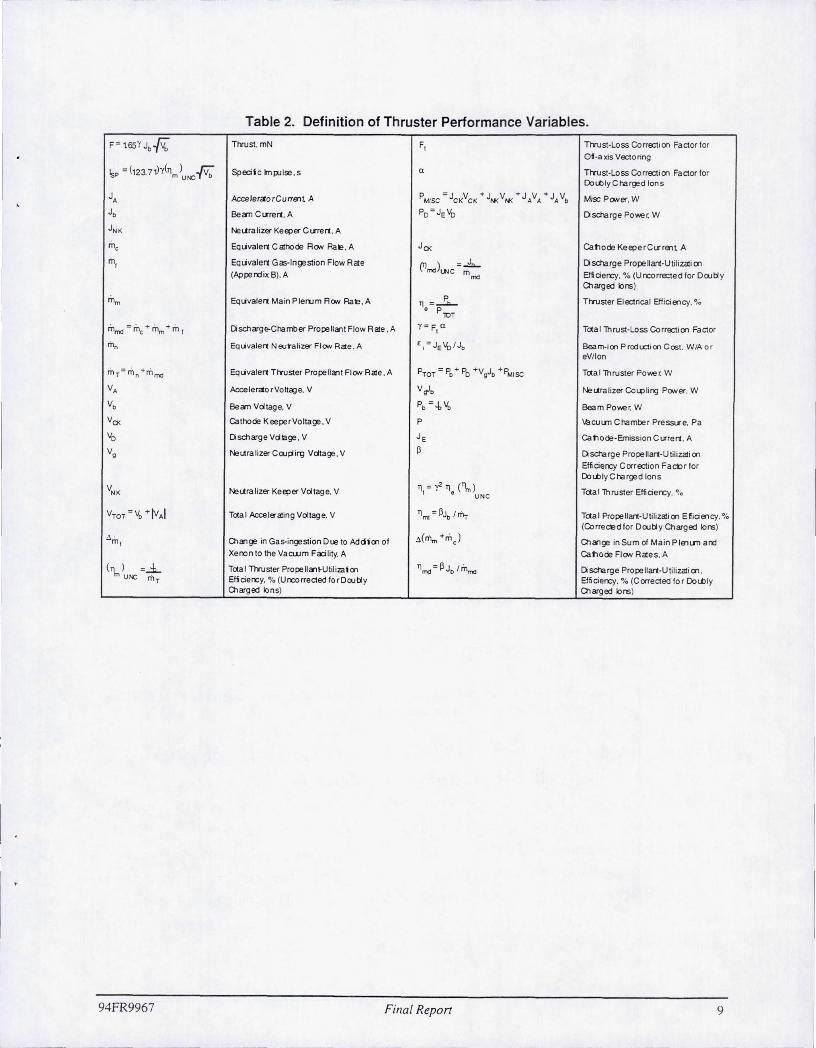
evaluation of the 25- and 30-cm-diam thrusters. Table 2 provides definitions of the various

current and VOltage symbols used in Figure 6. Table 2 also provides definitions of thruster

performance variables, including input power, thrust, specific impulse, and thruster efficiency.

2.3 PERFORMANCE EVALUATION

Performance evaluation of the NASAlHughes common thruster SIN 2 was conducted using

the standardized procedure developed under this contract and reported in the final report2 for

Phase 1. This procedure consists of operating the thruster for two hours at high discharge power

and then measuring the variation of propellant-utilization efficiency with beam-ion-production

cost as the latter is reduced to its minimum value. For each operating point, the cathode and

main flow rates are adjusted to maintain the discharge voltage and beam current at their desired

values.

Figure 7 shows the performance of the NASAlHughes common thruster SIN 2 operated at a

discharge voltage of VD = 28 V and beam currents of h = 1.45 A and 3.22 A. These discharge

voltage and beam-current values were used to provide a comparison with the 30-cm-diam lab

model thruster that was evaluated under Phase 1 of this contract. At J b = 1.45 A, the minimum


"""4614 £J L .. --y . T ...

. :lI -:.

Figure 4. Computerized data-acquisition system used for performing Langmuir-probe measurements.

94FR9967 Filial Repon 6

---

-~~---- --- - - -

9012-<l4·147R1

O.6-m-DIAMETER VACUUM CHAMBER

~ FLOW-RESTRICTING MASK

ROTATABLE

I CATHooJ SPUTIER

PYROMETER SHIELD

~

U QUARTZ WINDOW

GLASS RGA WINDOW

Figure 5. Schematic diagram of O.6-m-diam cryopumped vacuum chamber.


+

94FR9967

+ +

+

DISCHARGE POWER SUPPLY

KEEPER POWER SUPPLY

SIDEWALL ANODE

SCREEN ANODE

II

II

II

r-~~----------------~ JSG ~+-----------------------J

;::::::::1 •

J + b r----------------------+-+~

J A 1-+ _____________________ -J

Figure 6. Electrical schematic of thruster test console.

Filla! Repon

88 12·Q4· 18RJ

NEUTRAUZER KEEPER

POWER SUPPLY

8

------ .. __ .- .. - ----

Table 2_ Defin ition of Thruster Performance Variables.

F= t65Y Jb -/V: TtnJst. mN F, Th'ust-Loss Correcti on Factorior Of-axis Vectoring

is? = (123.7VY(11) .rv; SpeciSc m pl lse.s a Th'ust-Loss Correction Factor for m UN: b

DolblyCharged Ions

JA Acceler<forCurrm l A PM1SC = JCKVCK + J/'I(V/'I( + JAVA + JA Vb MiscPo.ver. W

Jb Be<ro Cu-rert . A Po = JeVo Dscharge Pov.er. W

JNK NeLiralizer Ke eper Cu-rert . A

me Equvalert Calhode Ro.v RaE . A JCK Catlode KeeperCt.rrenl A

ri'li Equvalert Gas-Ingestion Flow Rale (11rrd)UNC

=~ Dscharge Propeliart-UtiliZaiion

(Apperd ix B). A m"" Efticiercy. % (Uncorrected for Drut; y Olarged Ions)

mm Equvalert Main P lerum RON RaE . A TI=~ • PlOT

TtnJster EI ectrical Bfici e:l cy. %

. - ' + . + ' mmd - mc mm m, Dscharg~Chamb er Prope llant Flow Rale . A y = F,a Tcta l lhrust-Loss Correction Factor

ri1" Equvalert N ruralizer Flo.v Rale. A E , = Je Vo l Jb Beam-iCYl Produ:ticn Cost. W/Aor eV/lon

. - ' + ' mT- mn mmd Equvalert TtnJster Prope llanl Flo.v Rale. A PTOT = PD + Po +VgJb +PM1SC Tcta l lhruster Pov.er. W

VA Aooeler<fO rVoltage. V Vglb Ne Lira lizer Co<.plirg PONer. W

Vb Be<ro Voltage. V Pb = 4, I.\, Beam Pov.e r. W

VCK Cathode KeeperVoltage . V P Vacuum Chamber PreSSU'e. Pa

Vo Oscharge Volage . V J e Ca trode-Emission Ct.rrert . A

Vg NeLiralizerCrupirg Voltage . V P Oscharge Propeliart-UliliZaii on Efficiercy Correction FaCtl r for DolblyCharged Ions

VNK NeLiralizer Keeper Voltage. V 11 = y2 11 ('\,, )

I e UNC Tctallhruster Efficiercy. %

VTOT =1.\, + ivAI Tctal AcceIe-a1ing VoItag e. V TIm, = PJb Iffir Tctal Propellart-Utilizali on E!iciency. % (CorrecEd for Drut;y Charged Ions)

~ . m l Olange in Gas-ingestion Due to Addion of t.(~ +m e) Olcnge in Sum of Ma in Plmt.rn ard

Xenon to the Va cuum Faci lity. A Ca tl ode Flo.v Rales. A

('\" ) =..:1.... TOCa l Ttruster Propell an~Util i zal on Tlmo=PJb Immo Oscharge Prope liart-UtiliZai i on . UNC mT Efticiercy. % (Uncorrected for Dru t; y Efi ciercy. % (C orrected fo r Dolbly

Olarged Ions) Olarged Ions)


9412-04-101 250~-------------------------------------------'

-Z o 200 § CI) -t-"' en o u z o roo 150 U ::> c o a: a.

I

Z o

I

:E ~ 100 w m

VD = 28 V

R =0.8

- COMMON THRUSTER SIN 2

.",," HUGHES LAB-MODEL THRUSTER

Jb = 1.45 A

VTOT = 1100 V,

COMMON THRUSTER

VTOT = 1000 V,

LAB-MODEL THRUSTER

Jb = 3.22 A

VTOT = 1550 V,

COMMON THRUSTER

VTOT = 1350 V,

LAB-MODEL THRUSTER

• , .... .. ' .....

Jb = 3.22 A 1.45 A ,--.\.....-, r"--l

50~--~--~--~----~--~--~----~--~--~--~

20 30 40 50 60 70 80 90 100 110 120 DISCHARGE PROPELLANT - UTILIZATION EFFICIENCY, (%)

(UNCORRECTED FOR DOUBLY CHARGED IONS)

Figure 7. Discharge-chamber performance curve documented for NASAfHughes common thruster SIN 2 and the Hughes lab-model thruster. (Data corrected for gas ingestion.)

beam-ion-production cost of the NASNHughes common thruster is cj = 120 eVlion and the

maximum propellant-utilization efficiency (uncorrected for doubly charged ions) is

(T)md) unc = 87%. At Jb = 3.22 A, the minimum beam-ion-production cost of this thruster is cj =

100 eVlion and the maximum propellant-utilization efficiency is (Tlmd) unc =103 %. Figure 7

presents similar performance data obtained under Phase I using the Hughes lab-model thruster.

Figure 8 shows the beam profile of thruster SIN 2 measured at the "knee" of the performance

curve (Cj = 150 eVlion) for a beam current of Jb = 1.45 A. The computed beam-flatness

parameter is F = 0.45, which is approximately equal to that which was measured for the 30-cm

diam lab-model thruster under Phase 1 of this contract.

94FR9967 Final Repon 10

• I

F = 0.45 Jb = 1.45 A

Cj = 150 eV/ion

9312·04·055

PROBE CURRENT

""""< 0----;;'THRUSTER RADIUS

i

Figure 8. Beam-current-density profile measured in NASAlHughes common thruster SIN 2.

Figure 9 presents performance data obtained in the HRL test facility for the NASAlHughes

common thruster SIN 2 operated at the conditions specified by NASA - LeRC. Figure 10 and

Tables 3(a) and 3(b) compare the performance data presented in Figure 9 with similar results that

were obtained with this same thruster in the NASA - LeRC test facility. There is excellent

agreement in the baseline beam-ion-production cost for all beam currents. However, there is a

noticeable increase in the maximum propellant-utilization efficiency for the performance

measurements obtained at Hughes (at least for the higher beam currents). On the basis of the

flow-meter calibration results presented in Appendix A, we cannot attribute the observed

differences in maximum propellant utilization to any systematic error in the measured flow rates.

Repeatability of the performance data obtained at Hughes is shown in Figure 11 , and Figure 12

shows corresponding repeatability results obtained by NASA. The repeatability of thruster

performance data is within about ±3% in both the Hughes and NASA test facilities.

94FR9967 Filial Repon II

- ---_ ._--

9312-{)4-056 250~------------------------------------------'

-§ 200 § (l) -...,:

en o u z o t; 150 ;:) c o a: Cl.

I

Z o .. ~

~ 100 al

VD = 28 V

Jb = 0.8 A

VTOT = 700V

R = 0.8

Jb = 1.2A

VTOT =850 V R =0.8

O.SA

1.2 A

Jb = 1.45 A

VTOT= 1100 V R= 0.8

Jb = 3.22 A

Jb = 3.22 A

VTOT = 1550 V

R = 0.8

50 I 20 30 40 50 60 70 SO 90 100 110 120

DISCHARGE PROPELLANT -UTILIZATION EFFICIENCY, (%) (UNCORRECTED FOR DOUBLY CHARGED IONS)

Figure 9. Performance data for the NASAlHughes common thruster SIN 2 operated at Hughes.


9312'{)4-057 250.-------------------------------------------,

'2 200 o ~ Q) -.... ~

CJ)

o (.)

z e 150 (.) :::l C o a:: c..

I

Z o -I

~ 100 w CD

VD = 28 V

R = 0.8

HUGHES FACILITY

NASA FACILITY

~~~ ~~ ~ ~~ ~~ . ~ ~. - ~~.~.~---~-.. -.... --.•..... --.-

0.8A . , • ,1.4,5~ • . . D.. .

4.

.. fi .t;s."

Jb = 3.22 A I

8 ts ....

d P 1:::s.. •.•.•.••

.. ..............

. .. Ff .,

.,' ... -.

Jb = 0.8 A

VTOT= 700 V

Jb = 1.45 A

VTOT = 1100 V

Jb = 3.22 A

VTOT = 1550 V

50~--~--~--~----~--~--~~--~--~--~----~

20 30 40 50 60 70 80 90 100 110 120

DISCHARGE PROPELLANT 4.JTILIZATION EFFICIENCY, (%) (UNCORRECTED FOR DOUBLY CHARGED IONS)

Figu re 10. Comparison of performance data obtained at LeRC and Hughes for common thruster SIN 2.


Table 3(a). Listing of Thruster SIN 2 Performance Data Obtained in Hughes Test Facility.

9612·15-016

Jb = 3.22 A

p Jb Vb JA VA Jo Vo Jf'I( VNK Vg

. . . (11 mo)uNC mm mc mn tj

x 10-5 TORR (A) (V) (mA) (V) (A) (V) (A) (V) (V) (seem) (seem) (seem) (W/A) (%)

1.6 3.22 1240 20.3 310 1&6 28.00 2.0 12.0 12.23 43.1 2.75 2.82 161.4 104.8

1.6 3.22 1240 20.94 310 17.3 28.00 2.0 11.75 12.05 44.3 2.42 2.81 150.1 102.4

1.6 3.22 1240 21.94 310 16.0 28.08 2.0 12.43 12.58 45.7 2.14 2.82 140 100

1.6 3.22 1240 23.2 310 15.0 28.07 2.0 12.44 12.97 47.4 1.98 2.82 130 96.9

1.7 3.22 1240 25.3 310 13.5 28.08 2.0 12.8 13.53 50.4 1.70 2.82 118 91.98

1.8 3.22 1240 26.9 310 13.6 28.05 2.0 12.74 14.18 51.6 1.71 2.81 118 9.8

1.9 3.22 1240 31.1 310 125 28.03 2.0 12.51 13.40 57.6 1.45 2.81 109 81.1

2.4 3.22 1240 46.2 310 11.7 28.04 2.0 12.5 14.4 74.6 1.18 2.81 102 63.2

9612·15·015

Jb = 1.45 A

P J b Vb J A VA J O Vo J NK VNK Vg • .

mn ll1 )

mm mC tj mO UNC IX 10-5 TORR (A) (V) (rnA) (V) (A) (V) (A) (V) (V) (seem (seem) (seem) W/A) (%)

0.99 1.45 880 8.75 220 7.83 27.96 2.0 14.56 14.46 22.1 2.69 2.81 151 86.84

1.0 1.45 880 8.80 220 7.23 28.00 2.0 14.4 11.76 23.16 2.33 2.81 140 84.46

1.1 1.45 880 9.76 220 6.24 27.95 2.0 12.47 12.69 26.4 2.13 2.81 130 75.47

1.2 1.45 880 12.9 220 6.19 28.03 2.0 13.84 18.8 32.5 1.68 2.81 120 63.0

9612·15·014

Jb = 0.8 A

P Jb Vb JA VA Jo Vo JNK VNK Vg

. . . LTl ) mm mc mn tj mO UNC

X 10-5 TORR (A) (V) (rnA) (V) (A) (V) (A) (V) (V) (seem) (seem) (seem) (W/A) (%)

1.1 0.8 560 5.39 140 5.60 28.04 2.0 15.46 14.47 9.7 5.0 281 196.2 80.34

0.7 0.8 560 4.58 140 5.26 28.00 2.0 15.53 14.6 10.7 4.4 281 184.1 78.57

0.7 0.8 560 4.70 140 4.89 28.05 2.0 15.46 14.4 12.7 3.26 281 171.4 74.4

0.8 0.8 560 6.43 140 4.26 28.07 2.0 15.65 14.17 19.9 1.65 281 149.5 55.14

94FR9967 Fina! Report 14

r -!

Table 3(b). Listing of Thruster SIN 2 Performance Data Obtained in LeRC Test Facility.

9612-1S-Q16Rl

Jb = 3.22 A

p • • . (11 mo)uoc Jb Vb JA VA Jo Vo JNK VNK Vg mm mc mn Ej

X 10-5 TORR (A) (V) (mA) (V) (A) (V) (A) (V) (V) (seem) (seem) (seem) (W/A ) (%)

0.87 3.22 1255 14.0 299 21.8 2B 1 12.8 18.3 43.1 4.62 3.34 162 99.2

0.8 3.22 1254 14.0 304 21.2 2B 2 13.4 19 45.13 4.06 1.02 156 97.3

0.82 3.22 1259 14.0 303 20.4 28.1 2 13.5 19 46.01 3.57 1.02 150 96.53

0.84 3.22 1260 14.5 304 19.4 2B 2 13.2 18.8 47.53 3.10 1.02 141 94.2

0.87 3.22 1263 16.0 303 18.2 2B 2 13.0 18.8 50.5 2.58 1.02 130 90.9

1.3 3.20 1259 :E.O 301 15.0 2B 1 12.0 18.2 77.06 1.07 3.33 103 60.9

9612-1S-01SRl

Jb = 1.45 A

P Jb Vb JA VA Jo Vo JNK VNK Vg • . • l l1 mO)UNC mm mC mn Ej

Ix 10-5 TORR (A) (V) (mA) (V) (A) (V) (A) (V) (V) (seem (seem) (seem) W/A) (%)

0.48 1.44 893 4.5 217 11 27.9 1 14.0 18.0 20.39 2.97 3.36 185 91.4

0.48 1.45 889 4.5 217 10.5 28.0 1 14.0 18.0 21.53 2.41 3.36 175 89.9

0.5 1.45 892 5.0 218 10.0 28.0 1 14.0 18.0 22.43 1.86 3.36 165 88.6

0.52 1.45 895 5.5 218 9.3 28.0 1 14.0 18.0 24.18 1.49 3.36 152 83.8

0.55 1.45 897 6.0 220 8.89 27.9 1 14.0 18.0 25.69 1.41 3.36 143 79.4

0.61 1.46 896 7.5 215 8.39 28.0 1 14.0 18.0 29.35 1.1 9 3.35 133 70.9

1.4 1.49 888 35.0 224 7.8 28.0 1 14.0 19.0 84.01 0.42 3.34 119 26.2

9612-1 S-014R1

P Jb Vb JA VA Jo Vo JNK VNK Vg • • • l l1mo)UNC mm mC mn Ej

X 10-5 TORR (A) (V) (mA) (V) (A) (V) (A) (V) (V) (sccm) (seem) (seem) (W/A) (%)

0.36 0.8 549 4.0 146 6.6 27.9 1 14.5 20.8 11.93 2.23 1.0 202 83.6

0.36 0.8 546 4.0 147 6.4 28.0 1 19.2 27.0 12.31 1.92 1.02 196 83.2

0.38 0.8 539 4.0 148 6.0 28.0 1 21.0 28.7 13.2 1.60 1.01 182 80.0

0.39 0.79 549 4.5 151 5.6 28.0 1 13.8 21.0 14.46 1.30 1.01 170 74.2

94FR9967 Filial Report 15

9312{)4-058 250~--------------------------------------------~

'2 200 o ~ ~ ....(J)

o ()

z o i= 150 () :J C o a: a..

I

Z o

I

~ <t 100 w CD

Vo = 28 V R =0.8 VTOT = 1550 V Jb = 3.22 A

• DAY 1 TESTING

o DAY 2 TESTING

50~--~--~--~--~----~--~--~--~--~--~

20 30 40 50 60 70 80 90 100 110 120

DISCHARGE PROPELLANT-UTILIZATION EFFICIENCY, (%) (UNCORRECTED FOR DOUBLY CHARGED IONS)

Figur e 11. Typical repeatability of performance data for the NASAlHughes common thruster SIN 2 operated at Hughes.

94FR9967 Filla! Report 16

I .

-c:: 0

::::::: > (1) -~~

en 0 u z 0 ~ u ::> c 0 a: a.

I

z 0

I

:2 ~ W ED

9312-04-059

200

• DAY 1 TESTING

180 0 DAY 2 TESTING

VD = 28 V VT = 1550 V

160 Jb = 3.22 A

140

120

100

80L-------~------~--------~------~------~ 0.2 0.4 0.6 0.8 1.0 1.2

DISCHARGE PROPEllANT UTILIZATION EFFICIENCY, (%) (UNCORRECTED FOR DOUBLY-CHARGED IONS)

Figure 12. Typical repeatability of performance data for the NASAlHughes common thruster SIN 2 operated at LeRC.

2.4 BEAM DIAGNOSTICS

Figure 13 compares the beam-current-densi ty profi les measured in the NASA and Hughes

test facilities for the common thruster SIN 2 operated at a beam current of h = 0.8 A. The

Hughes measurements were obtained using a movable Faraday probe located downstream of the

accel (negative) electrode. The probe data were recorded on an x-y plotter and then digitized

using a tablet digitizer. The integrated beam current is shown to have a value of 0.74 A, which is

within 7.5% of the measured value of the beam current (Jh = 0.8 A). The beam-flatness


parameter has a value of F = 0.44. The NASA Faraday-probe data (half-scan shown in

Figure 13) were taken with a Faraday probe located 25.4 mrn downstream of the aceel electrode.

and therefore indicates a slightly lower current density. Figure 14 presents a similar comparison

of the current-density profiles for the common thruster SIN 2 operated at the conditions of

NASA's 5-kW life test. 3 The beam-flatness parameter of F = 0.41 is somewhat less than that

which has been measured for the 25- and 30-cm-diam XIPS thrusters at a beam current of

Jb = 3.22 A (F = 0.54 and 0.5, respectively) .

-N E ()

~ E ->~

!:: en z w C IZ W 0: 0: :J ()

W CD o 0: Cl.

9312·04·060

4~--------------------------------------------~

3

2

1

Jb = 0.8 A

Vo = 28 V

VTOT = 700 V R = 0.8

• HUGHES FACILITY, PROBE 1.6 mm DOWNSTREAM OF THE ACCEL ELECTRODE

o NASA FAOLlTY, PROBE 25.4 mm DOWNSTREAM OF THE ACCEL ELECTRODE

F = 0.44 (Jb) FARADAY = 0.74 A

PROBE ........... ,.,. .. , .. • • •

• • • • • \ '\

o~--__ ~~~--________ ~ ________ ~ ____ ~~ __ ~ -20 -10 0 10 20

RADIAL PROBE LOCATION, (em)

Figure 13. Comparison of beam-current-density profiles obtained at LeRC and Hughes for common thruster SIN 2 operated at a power level of600 W.

94FR9967 Fillal Report IH

9312·04-06 1

8r---------------------------------------------.

-N E (.)

< E ->=' I-en z w

6

c 4 I-Z w a: a: => u w m o 2 a: £:L

• HUGHES FACILITY, PROBE 1.6 mm DOWNSTREAM OF THE ACCEL ELECTRODE

o NASA FAOLlTY, PROBE 25-4 mm DOWNSTREAM OFTHEACCELELECTRODE

J b = 3.19A •• (Jb) FARADAY= 2.93 A

(

•••••• ~ F=D.41

•• PROBE VD = 28 V •

\ VTOT = 1550 V: : R = 0.8 I ~

• I

II :{

.iJ :J I

J

• • • • • • • • • • • • • • • • • • • • • • •

\ • ...

O~--~~--~----------~----------~----~--~ -20 -10 o 10 20

RADIAL PROBE LOCATION, (em)

Figure 14. Comparison of beam·current-density profiles obtained at LeRC and Hughes for common thruster SIN 2 operated at a power level of 4.6 kW.

The doubly charged ion fraction of the NASAlHughes common thruster SIN 2 was measured

using an ExB probe. Measurements were obtained at an operating condition of Jb = 3.22 A,

corresponding to the two operating points indicated as solid dots in Figure 15 (propellant

utilization efficiencies of (llmd) unc = 104.1 % and 92.6%, respectively). Tables 4 and 5

summarize the thrust-loss parameters obtained from the ExB-probe measurements at the two

operating points. The doubly charged ion fraction measured at a propellant-utilization efficiency

of (llmd)unc = 104% is quite high, having an average value of J++IJ+= 0.27 . Reducing the

propellant-utilization efficiency to (llmd)unc = 92.6% reduces the doubly charged ion fraction to a

more-reasonable average value of J++/J+ = 0.15.


9312-{)4-062 250~--------------------------------------------~

-§ 200 :.:::: > (1) -t-=' en o ()

z o I- 150 () :::> c o ex:: c.. :Z o "j"

:E <! w co

100

Jb = 3.22 A

VD = 28 V R =0.8 VTOT = 1550 V

#1

50~--~--~--~----~--~--~--~----~--~--~

20 30 40 50 60 70 80 90 100 110 120

DISCHARGE PROPELLANT -UTILIZATION EFFICIENCY, (%) (UNCORRECTED FOR DOUBLY CHARGED IONS)

Figure 15. Performance conditions (solid symbols) under which ExB-probe data were obtained for common thruster SIN 2.


.. _ _ . ~ . . , _____ c··· ._ .. _. _. ___ .

Table 4. Summary of ExB Probe Data (Point #1 in Figure 11) :

Input Data !

<1>P r= 0.75 R r = 0.50 R r = 0.25 R r = 0.00 R j

(deg) J+(nA) J++ (nA) J+ (nA) J++(nA) I J+(nA) J++(nA) J+(nA) I J++(nA) ! I

-25.0 0.0034 0.0017 0.0029 0.0016 0.0020 0.0015 0.0017 i 0.0015 : I ,

-20.0 0.0086 0.0030 0.0056 0.0022 0.0036 0.0021 0.0024 i 0.001 7 I

-15.0 0.0310 0.0055 0.0124 0.0040 0.0065 0.0033 0.0036 I 0.0023 i I I -10.0 0.0992 0.0115 0.0635 0.0158 0.0273 0.0085 0.0133 I 0.0043

I I

-5.0 0.1172 0.0149 0.2138 0.0693 0.1124 0.0487 0.0646 0.0279

I 0.0 0.0485 0.0060 0.1698 0.0467 0.2123 0.1104 0.2019 0.1175

5.0 0.0124 0.0024 0.0428 0.0086 0.0942 0.0402 0.1423 0.0735 ! 10.0 0.0036 0.0015 0.0071 0.0023 0.0252 0.0067 0.0403 0.0146 I 15.0 0.0020 0.0013 0.0034 0.0019 0.0038 0.0023 0.011 5 0.0037 i

Summary of Thrust Parameters I I r= 0.75 R r= 0.50 R r = 0.25 R r = 0.00 R

j+ (mNcm2) 7.19 9.6132 9.03 8.20 I I

j++ (mNcm 2) 1.60 2.2937 3.88 3.97 i U++/j+) 0.22 0.2386 0.42 0.48

<1> (deg) 12.4 9.9401 9.85 9.63

a I Ft J+ + J++ I ~ J++ / J+

0.937 0.980 5.5 0.892 0.272

Table 5. Summary ofExB Probe Data (Point #2 in Figure 11)

Input Data

<1>P r = 0.75 R r = 0.50 R r = 0.25 R r = 0.00 R

(deg) J+(nA) J++ (nA) J+ (nA) J++(nA) J+(nA) J++(nA) J+(nA) J++ (nA)

-25.0000 0.0032 0.0014 0.0028 0.0014 0.0020 0.0013 0.0014 0.0013

-20.0000 0.0082 0.0019 0.0059 0.0018 0.0038 0.0017 0.0025 0.0015

- 15.0000 0.0345 0.0044 0.0051 0.0030 0.0072 0.0023 0.0039 0.0018

-10.0000 0.1236 0.0083 0.0095 0.0034 0.0448 0.0074 0.0144 0.0030

-5.0000 0.1544 0.0099 0.2847 0.0443 0.2092 0.0461 0.0939 0.0223

0.0000 0.0614 0.0037 0.0194 0.0288 0.2757 0.0657 0.2730 0.0766

5.0000 0.0154 0.0018 0.0520 0.0055 0.1117 0.0234 0.1945 0.0558

10.0000 0.0039 0.0014 0.0062 0.0019 0.0242 0.0035 0.0426 0.0076

Summary of Th rust Parameters

r= 0.75 R r=0.50 R r= 0.25 R r = 0.00 R

j+ (mNcm2) 8.1909 2.5715 10.5449 9.6943

j++ (mNcm2) 0.9204 0.6693 2.2960 2.8557

U++/j+) 0.1124 0.2603 0.2177 0.2946

<1> (deg) 11 .3081 5.4447 8.4418 8.741 1

a Ft J+ + J++ ~ J++ / J+

0.96148 0.98414 4.68528 0.93424 0.15143

94FR9967 Fillal Report 21

_. J

Table 6 is a summary of the thruster performance parameters (thrust , specific impulse .

efficiency, and total power) computed using the tabulated electrical parameters and the thrust

loss correction factors listed in Tables 4 and 5. Note that at the operating condition of ]b = 0.8 A

we could not detect the presence of any doubly charged ions. (The detection value of our ExB

probe is believed to be :::::1 %.

Table 6. Performance Data for NASAlHughes Common Thruster SIN 2

Jb VD Vb VA J++/J+ £j Pb PTOT TI e (Tlmd)unc (Tlm)unc F i I

(A) (V) (V) (V) (%) (eV/ion) (kW) (kW) (%) (%) (%) Y (mN) i 3.22 27.9 1240 -310 27.2 161.2 4.0 4.61 86.6 104.1 98.51 919

1

172 i 3.22 27.96 1240 -310 15.1 116.8 4.0 4.48 89.13 92.6 88 .0 .946 177 i

i 0.8 28.0 560 -140 0 196.0 0.448 0.651 68.8 80.3 67.6 .983· ; 30.7 i

I

· Uses thrust loss correction factor for beam divergence corresponding to Jb = 3.22 A. ! Electrical Data for Common Thruster SIN 2

I ,

JA (mA) VNK (V) Vg (V) J NK (A) \ :

21 .5 10.87 12.0 2.0 I 27.2 11.0 13.0 2.0 I

! 5.23 15.36 13.95 2.0

Nomenclature:

JA ::: accel current £j = beam-ion-production cost

Jb ::: beam current Pb = beam power

J NK = neutralizer keeper current PTOT = total power

Vg ::: coupling voltage Tl e ::: electrical efficiency

VD ::: discharge voltage y = thrust loss correction factor

Vb ::: beam VOltage F thrust

VA ::: accel voltage Isp specific impulse

VNK ::: neutralizer keeper voltage

J++jJ+ ::: rat io of doubly to singly charged ion currents

(uncorrected for doubly charged ions)

(Tlmd)unc ::: discharge propellant-util ization efficiency (uncorrected for doubly charged ions)

(Tlm)unc ::: total thruster propellant-utilizationefficiency (uncorrected for doubly charged ions)

2.5 ION OPTICS PERFORMANCE

The perveance of ion-optics assembly SIN 907 used on the NASAlHughes cornmon thruster

SIN 2 was obtained over a wide range of beam current, using the measurement procedure

described in the final report2 for Phase 1. The beam voltage was swept over a range of about

600 V, and both the beam voltage and accel current were recorded on an x-y plotter. Figure 16


-- ------~~-

,--I I

I

50

- 40-« E -.a: ..., ~~

ffi 30 c: c: :::I U ...J W U u 20 «

« E 10 LO co ~

~

mm = 17.3 seem

me = 2.47 seem

mn = 2.68 seem

Jb=0.6A } Vo = 28 V

JE = 3.47 A

VA = -140 V

/ (Vb) min= 385 V

9312-04-063

O~----~~----~------~------~------~----~

300 400 500 600 700 800 900

BEAM VOLTAGE, Vb' (V)

Figure 16. Accel-currentlbeam-voltage characteristic for ion optics SIN 907 operated on the NASAlHughes common thruster SIN 2.

shows the resulting variation of acce1 current with beam voltage for the common thruster SIN 2

operated at a beam current of Jb = 0.6 A. The initial setpoints for the beam current, discharge

voltage, cathode-emission current, and acce1 voltage are shown in the figure.


I I

I

The minimum beam voltage (Vb)min was determined from the recorder trace by locating the

value of beam voltage at which the slope of the accel-currentlbeam-voltage characteristic was

equal to 0.1 mAIV. The operating beam voltage, Vb, was then taken as 200 V above (Vh)min .

The ion-optics operating voltage, VT, was then defined as:

(1 )

The operating value of the net-to-total accelerating-voltage ratio was calculated as

R = Vb/VT- Table 7 summarizes the values of (Vb)min , V A, VT , and R as a function of beam

current.

Table 7. Perveance Data for Ion Optics SIN 907

Jb(A) (Vb)min (V) Vb = (Vb)min + 200 (V) VA (V) VT = (Vb)min +1 V A 1+ 200 (V) R , :

0.6 385 585 -140 I 725 1 0.81

0.8 465 665 -140 805 0.B3

1.2 475 675 -220 B95 0.75

1.B 660 860 -220 10BO O.BO

2.4 685 885 -310 1195 0.74

3.0 820 1020 -310 1330 0.77

3.6 965 1165 -310 1475 0.79

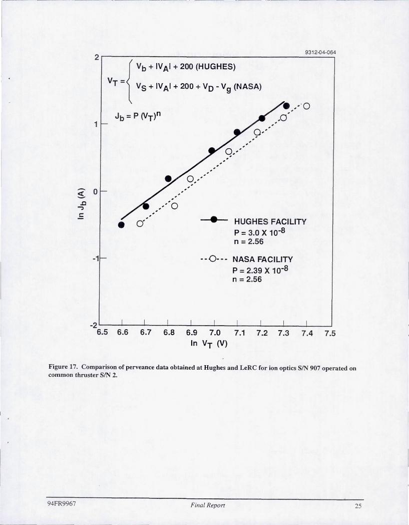
Figure 17 is a perveance plot of the data presented in Table 7. For comparison, similar data

obtained at NASA are also shown. There is excellent agreement between the Hughes and NASA

results for the power-law parameter, n. However, the actual perveance, P, is slightly greater for

the data obtained at Hughes. The Hughes data indicate a lower total voltage requirement of as

much as 125 V.


I

--- ,----

9312'{)4-064 2r---------------------------------------------~

Vb + IVAI + 200 (HUGHES)

Vs + IVAI + 200 + Vo - Vg (NASA)

1

~ 0 .c ..., c

• -1

• HUGHES FACILITY P = 3.0 X 10-8

n = 2.56

- -0- -- NASA FACILITY

P = 2.39 X 10-8

n = 2.56

-2~--~--~----~--~----~--~--~~--~--~--~

6.5 6.6 6.7 6.8 6.9 7.0 7.1 7.2 7.3 7.4 7.5 In VT (V)

Figure 17. Comparison of perveance data obtained at Hughes and LeRC for ion optics SIN 907 operated on common thruster SIN 2_

94FR9967 Final Reporr 25

Section 3 COMPONENT TECHNOLOGY

3.1 DISCHARGE-CHAMBER SIMPLIFICATION

We explored the feasibility of eliminating the cathode-keeper electrode as a means of

simplifying the ring-cusp thruster and its power processor unit (PPU) , while at the same time

eliminating a pote,ntial erosion site3 within its discharge chamber. Figure 18 is a schematic of

the 30-cm-diam discharge-chamber simulator (operated without ion-beam extraction) that was

used in these tests. With the cathode-keeper assembly in place as shown, we ignited the

discharge plasma by applying a voltage directly between the cathode and anode. Two power

supplies were diode-summed to provide a high-voltage boost (s;: 1 kV) for ignition and a high

current (s;: 5 A) for sustaining the discharge plasma. During these experiments, the cathode

keeper assembly was electrically isolated and allowed to float. With 0.7 sccm of xenon flowing

through the cathode and ::::::23 sccm of xenon flowing into the discharge chamber, we

demonstrated repeatable discharge ignitions using a maximum high-voltage boost of only 90 V.

Steady-state operation was achieved at a cathode-emission current of JE = 5 A and a discharge

voltage of VD = 30 V.

~CATHO~CATHODE ----------------~~~ __ ~I I~ KEEPER

I I =1 VSOOS

VSOOST : 1 kV, :::::: 10 rnA

Vo : 50 V, 50 A

Figure 18. Electr ical schematic of discharge-chamber simulator.

94FR9967 Final Repon

951 2·04 '()19

FLOWLIMITING "MASK"

I

26

~ - _ ._----- ---------

Next, we removed the enclosed-type keeper in a 30-cm-diam lab-model thruster. and the

keeper supply in our laboratory test console was diode-summed with the discharge supply to

provide a high-voltage boost capability. We successfully started and operated the lab-model

thruster in this configuration (with ion-beam extraction). The adequacy of our high-voltage

recycle algorithm for this "keeperless" operation was also demonstrated. Although our recycle

algorithm cuts the discharge current back to zero while reestablishing the screen and accel

voltages, the discharge current provided by the high-voltage starting supply was adequate to keep

the cathode from extinguishing during :::::2-sec-duration recycles .

3.2 CATHODE PERFORMANCE

A discharge-cathode assembly provided by NASA was evaluated usmg the discharge

chamber simulator shown in Figure 18. The evaluation consisted of conditioning the cathode

insert according to a procedure specified by NASA, and then measuring the cathode temperature

as a function of discharge current and cathode flow rate.

Figure 19 shows a schematic diagram of the cathode assembly that was provided by NASA.

consisting of a 6.35-mm-diam hollow cathode equipped with an insert, heater, and radiation

shield. The orifice diameter in the NASA-provided cathode was 0.762 mm. An R-type

thermocouple (PUPt -13 % Rh) was spot welded to the side of the cathode tip, and a Granville

Phillips thermocouple gauge and readout were used to measure the pressure within the cathode.

The discharge-chamber simulator was cleaned by grit-blasting its interior and then washing it

with acetone and alcohol prior to installation of the NASA-furnished cathode. Plastic gloves

were used to handle all cathode and discharge-chamber parts, and the xenon flow lines were

baked out using a heat gun.

The cathode evaluation was conducted in the O.3-m-diam cryopumped vacuum chamber; a

schematic of this chamber is shown in Figure 20. The vacuum chamber is equipped with a

Dycor Model MA200FG residual gas analyzer for measuring the partial pressures of various

gases, induding water vapor, nitrogen, and xenon. The typical background (no flow) pressure in

this chamber is ::::: 6xlO-8 Torr.

3.2.1 Cathode Conditioning

Conditioning of the cathode insert was performed using a procedure provided by NASA.

Table 8 shows the cathode-heater currents and voltages (Ich and V ch, respectively) , as well as the

cathode temperatures (T c) that were measured during the low- and high-power phases of the

conditioning sequence. The high-power conditioning temperature of T c=1044°C was used as the

cathode temperature for igniting the discharge in all subsequent testing.

94FR9967 Filla! Repon 27

BARIUM ALUMINATE IMPREGNATED

TUNGSTEN INSERT

XENON GAS FLOW

RADIATION SHIELDING

9012-15-075

SWAGED TYPE R HEATER THERMOCOUPLE

CATHODE ORIFICE

Figure 19. Schematic of discharge cathode in NASAlHughes common thruster.

ROTATABLE SPUTTER SHIELD

C9012-15-71R5

QUARTZ WINDOWS

COMMON THRUSTER CATHODE

GRANVILLE-PHILLIPS PRESSURE GAUGE

I

GLASS WINDOW TO RGA

Figure 20. Schematic of 0.3-m-diam vacuum-chamber setup.


XENON GAS

FLOW

DISCHARGE CHAMBER

28

Table 8. Cathode Conditioning Log

Cathode Conditioning i Power Level Ich (A) Vch (V) Pch (W) Tc (0C) t.t (h) I

Low 4.32 3.4 14.6 532 I 3 !

Off 0 0 0 - 0.5

High 7.92 9.14 I 72.4 1044 1.0 I

3.2.2 Discharge Ignition

The cathode was evaluated over a five-day period. Each day the discharge was ignited by

first applying the heater current specified in Table 8 to achieve a cathode temperature of l044°C.

After a selected flow rate was established, voltage was applied between the cathode and anode to

achieve ignition and establish the discharge. This was accomplished by using a high-voltage

boost power supply (1 kV @ :::::10 rnA) diode-summed with a low-voltage (50 V) , high-current

(50 A) power supply, as shown in Figure 18.

Table 9 shows a history of the discharge-ignition characteristics. On the first day of cathode

operation, (following the previous day ' s cathode-conditioning sequence) a high xenon flow rate

(i.e., gas burst) was required to initiate the discharge. For all subsequent cathode operation,

normal ignitions were achieved at the nominal flow condition (4 sccm or 8 sccm), without the

use of the high-voltage-boost power supply.

Table 9. Discharge Ignition Log

Day Discharge Ignition Conditions

1 Abnormal Start Gas Burst VBoostRequired

2 Normal Start m = 4 seem Vo Only


4 Normal Start m =4seem Vo Only


3.2.3 Cathode Heater and Thermocouple Behavior

Prior to igniting the discharge each day, the IfV characteristics of the cathode heater, as well

as the thermocouple resistance, were measured to determine whether any changes in the

thermocouple and heater had occurred. Table 10 shows the measured cathode temperature for

the same heater power level.


Table 10. Cathode Heater Power Log

Cathode Heater Power I !

Day ICH (A) VCH (V) PCH (W) TT.C. (0C) I I

1 8.44 10.06 84.9 1044

2 8.44 10.0 84.4 1038

3 8.44 10.02 84.6 1040

4 8.44 10.04 84.7 1040

5 8.44 10.07 84.9 1039

• All measurements taken from cold start, (i.e., T c = 25°C at t = 0).

3.2.4 Temperature Measurements

Following ignition of the discharge, the variation of cathode temperature with emission

current was obtained for two different flow rates. The emission current was set to its maximum

value of JE = 25 A, and the temporal behavior of the cathode temperature was recorded to

determine when steady state had been reached. By our definition , the steady-state condition was

reached when the cathode temperature .was observed to change by less than 5°C over a 30-min

time period. The emission current was then reduced in 5-A increments (down to a minimum

value of JE = 5 A), with the steady-state temperature determined in the manner just described.

Figure 21 shows the temporal behavior of the cathode temperature for emission currents of 25,

20, and 15 A at a fixed flow rate of 4 sccm. At this flow rate, the emission current could not be

increased above JE = 25 A without the discharge voltage increasing to a value in excess of

V D = 40 V. Figure 21 indicates that for an emission current of JE = 25 A, the cathode

temperature initially rises to nearly I280°C, and then decreases to a steady-state value of I188°C

in a 45-min period. For the other two emission currents shown (JE = 20 A and JE = 15 A), the

steady-state temperature is achieved within a IS -min period.

Figure 22 shows the variation of the steady-state cathode temperature with emission current

recorded over a three-day period. The data indicate good reproducibility of measured

temperatures. Figure 23 shows the corresponding discharge voltages. For each of the cathode

temperature measurements shown in Figure 22, the cathode pressure was recorded using a

thermocouple gauge (see Figure 20 for location of the pressure gauge). Figure 24 shows good

reproducibility of the cathode pressure over the three-day testing period. The data indicate that

for fixed flow rate, the cathode pressure increases with emission current (cathode temperature) .

We explored this behavior further by using the ideal-gas law and the measured pressure (shown

in Figure 24) and temperature (shown in Figure 22) to calculate the xenon density in the cathode.


-- - -----------

-() ~

ill ((

~

t:( ((

ill CL ~ ill r-ill o o I

~ o

o .2 .4 .6 .8 1 1.2 1.4 1.6

ELAPSED TIME (h)

---_. -_. -_._------

1.8

9012-15-74

2

c.o ~ o

Figure 21. Strip-chart recording of cathode-temperature variation.

(The magnitude of the calculated densities may be in error because the pressure-gauge

manufacturer was unable to provide a factor for converting indicated pressures to true xenon

pressure). Figure 25 shows that the computed xenon density is approximately constant, as

expected, indicating that the observed cathode pressure is a function of temperature only (for

constant flow rate). Figures 26-28 contain cathode-evaluation data for the cathode operated at a

flow rate of 8 sccm. The data exhibit a behavior similar to that observed at a flow rate of 4 sccm.

Figure 29 shows the temporal variation of cathode temperature for a flow rate of 8 sccm and

a discharge current of 30 A. There is a linear decrease in temperature with time during the first

1.5 h, and then the cathode temperature reaches steady-state conditions. The data in Figure 30

show that the measured partial pressures of water vapor, nitrogen, and xenon, remain constant

and do not correlate with changes in cathode temperature.


.- -----------------------------

9312-{)4-065 1300~--------------------------------------------~

m= 4 seem

1200

-() 0 -W II: 1100 ::::> I-< II: W a.. ~ w • I-W 1000 c 2 I-< () • DAY 1

900 0 DAY 4

.6 DAY5

800~--------~----------~--------~----------~ o 10 20 30 40

EMISSION CURRENT (A)

Figure 22. Variation of cathode temperature with emission current (4 sccm flow rate).


9312-04-066 40~--------------------------------------------

m = 4 seem

0 • 30

-> -w (!)

~ ...J 0 > w 20 (!) c: ex: :I: () en c

• DAY 1 10 0 DAY 4

1:l DAY 5

OL---------~~--------~~----------~--------~ o 10 20 30 40


Figure 23_ Variation of discharge voltage with cathode-emission current (4 sccm flow rate).

94FR9967 Filia l Repon 33

93 12-{)4-068 1000.-------------------------------------------,

m = 4 seem

900

-~ ~ {:. E 800 --w a: :::> (J) (J) w a: a.. 700 w 0 0 ::I: ~ <t U 600 u -i= • <t DAY 2 ~ (J) 0 DAY 4

500 - L DAY 5

400~--------~----------~--------~----------~ o 10 20 30 40


Figure 24. Variation of cathode pressure with emission current (4 sccm flow rate).


.- --- - - - --------- -- - _ .. _. - ---_._.- -.-- ... ----

9312{)4-069 6~------------------------------------------~

m = 4 seem

5 /\ - ~ M

I (I ~ n. E 0 -LO

0r-

o 4 -or-

X W C 0 J: .... et 3 u z > t: en • DAy 2 z w 2 -

0 c DAY 4 z

L 0 DAY 5 z w x

1 -

o~----------~----------~----------~----------~ o 10 20 30 40

DISCHARGE CURRENT (A)

Figure 25. Calculated xenon gas density within discharge cathode (4 sccm flow rate).


9312{)4·070 1300~-------------------------------------------' .

m = 8 seem

1200 -

-U 0 -W II: :::J 1100 ~ ~ II: W a.. ~ w ~ w c 1000 -2 ~ ~ U

900 - • DAY 1

0 DAY 3

800~--------~--------~----------~--------~ o 10 20 30 40


Figure 26. Variation of cathode temperature with emission current (8 seem flow rate).


9312-04-071 40~-------------------------------------------'

,;, = 8 seem

30

-> -w

" ~ ..J 0 > 20 w

" a: <C ~ ~ ::J: 0 e 0 u en c

10

• DAY 1

0 DAY 3

o~----------~----------~----------~----------~ o 10 20 30 40


Figure 27. Variation of discharge voltage with cathode-emission current (8 sccm flow rate).

94FR9967 Fillal ReporT 37

- -- -- ---~

- ----r-

9312-04-072 8 ~------------------------------------------------, .

m = 8 seem . ,

-M I

E 6 • • (J • • - • Lt') • 0 0 0 T"" 0 T""

X W C 0 :J: r-<t 4 U z > r-en z w • DAY 1 c z 0 DAY 3 0 2 z w x

o~--------~------------~----------~----------~ o 10 20 30 40


Figure 28. Calculated xenon density within discharge cathode (8 sccm flow rate).

94FR9967 Filla! Report 3R

9312-04-073 1300~-----------------------------------------'

-U 0 -W II: ::> 1100 .... <t II: w 0..

m = 8 seem :a: w JD = 30 A .... w 1000 c 2 .... <t U

900

800L-----~------~------~------~------~1 ------~ o 0.5 1.0 1.5 2.0 2.5 3.0

ELAPSED TIME (h)

Figure 29_ Temporal variation of cathode temperature (8 seem flow rate).


9312-04-074

10-3 . m = 8 seem J o = 30 A

10-4• ~ •• .. • • • • (PTOTl Xe

VACUUM CHAMBER ION GAUGE

10-5 f--~ ~ {? - [ 0 DO OJ D D 0 D (PTOTl Xe - RGA W c: . ~ • •• .. • •• • Xe

:::> 10-6 r-en en w c: tl.

10-7 r-

• • • •• .. • • • N2

10-8 ( r-o 00 CD 0 o 0 o H2O

10-9~----~I------~I ----~I ------J~----~1----~ 0.0 0.5 1.0 1.5 2.0 2.5 3.0

ELAPSED TIME (h )

Figure 30_ Temporal variation of background partial pressure (8 seem flow rate)_


Section 4 LASER-INDUCED FLUORESCENCE

4.1 FEASIBILITY ANALYSIS

In laser-induced fluorescence, atoms are stimulated by an external resonant laser source. in

addition to the inherent stimulation by the electrons in the plasma. The LIF signal is independent

of the plasma conditions, provided the plasma does not significantly affect the density of the

ground-state atoms. We selected the ground state atomic transition process (A = 390.2 nm) for

molybdenum atoms that provided the largest fluorescence signal for a given laser power.

Plasmas produced in ion thruster discharge chambers are characterized as partially ionized

(-10%), low-pressure (-10-5-10-4 Torr) plasmas, with an average electron temperature of 2-5 e V

and plasma densities on the order of 1010-101Icm-3.4 For these plasma parameters, less than 1 %

of the molybdenum atoms sputtered from a surface exposed to the plasma are raised to excited

states as a result of collisions with electrons.4 In order to achieve a high signal-to-noise ratio

(large ratio of the laser-induced to collision-induced signals) in the laser-induced fluorescence

method, the excitation of molybdenum atoms must be dominated by laser photon absorption.

Therefore, we must determine the ratio of laser-induced to collision-induced excitation rates of

molybdenum atoms as a function of laser intensity. Note that the following equations employ

Gaussian units .

The rate for atomic stimulated excitation, Rre , is given in terms of the Einstein A coefficient

2 2 R (

. .) gj nn c IAjig re I ~ J =- 3

gj 2Xij (1 )

where gi and gj are the degeneracies for atomic levels i and j, respectively , I is the intensity of the

radiation, Aji is the Einstein A coefficient, and Xij is the energy difference between levels i and j.

The Doppler distribution function g, evaluated at line center of the transition, given by6

(2)

where k is Boltzmann's constant, MA and TA are the mass and temperature of the molybdenum

atom, respectively, and h is Planck's constant. Since the energy distribution of sputtered atoms

from a surface subjected to ion bombardment is -1-2% of the incident ion energy,7 kTA-l eV for

the conditions of our experiment.

A semi-empirical formula for the electron-impact (collision-induced) excitation rate between states i and j , Rp (i ~ j), is8


(3)

where me is the electron mass, Roo is the Rydberg energy (13.51 eV) , T e is the electron

temperature,Iij is the oscillator strength for the transition form level i to level j , g is the energy

averaged Gaunt factor (a correction factor) , ao is the Bohr radius, and lle is the electron density .

Under our operating conditions g is assumed to be unity .

The use of Eq. (3) assumes that the electron energies can be characterized by a local

Maxwellian energy distribution which has been shown to adequately describe the electrons in ion

thruster discharge chambers.

Equation (3) can be cast into a form that allows for a more convenient comparison to

radiative excitation by relating the oscillator strength to the Einstein A coefficient by5

3 2 mec Pz gjAji

I ij = 2e2g.x? I I)

(4)

In terms of fundamental constants and the spontaneous decay from the excited state, the

plasma excitation rate is given by

(5)

Assuming that the decay processes and rates are the same for atoms excited by either plasma

electrons or optical photons, the relative intensity of the LIF signal compared to the background

(plasma-induced) fluoresecence signal is given by the ratio of the excitation rates for the two

processes

(6)

For operating conditions where the Doppler width is larger thatn the laser linewidth, the

appropriate value of g to use is given by Eq. (2) . Assuming kTA=1 eV and 2nPzclXij = 3902 A yields g = 1.55x 10- lOs. In the experiment discussed later, we used an ultraviolet beam from a

Coherent 599 dye laser with an intensity of approximately 2 W/cm2. Equation (6) can then be

evaluated using the parameters ne= 101 I cm-3, kTe=3 eV, and Xij= 3.18 eV. This gives a value of

650 for the ratio RrelRp , which is large enought to provide ample signal for determining the

molybdenum density.

This calculation applies to the same volume of atoms for both excitation modes (plasma and

radiative). In paractice, the geometry of the measurement is very important and it is difficult to


, .

completely isolate the volume of atoms intercepted by the laser beam to avoid fluorescence

contributions from other regions where the excitation mechanism is solely collisional. Although

shielding was used in the experiment to minimize this additional contribution. a sizeable plasma

background signal was present. Therefore. a phase-sensitive detection technique. described in

Section 5.2, was employed and achieved a high signal-to-noise ratio. However, it was still

necessary to keep the background fluorescence contribution small in order to avoid saturation of

the detector.

Commercially available Ti:Sapphire lasers are much easier to maintain than a dye laser

system and would probably be selected as the optical source in a practical diagnostic station.

Using internal cavity doubling, these lasers can produce 200 mW of output power at 390 nm.

which is resonant with the lowest lying dipole-allowed ' molybdenum ground state transition . If

this beam is collimated to a I cm2 spot, the intensity 1 would be 200 mW/cm2. This gives a value

for RrelRp of 65 for the Ti:Sapphire laser, which should produce a reasonable signal-to-noise

ratio.

4.2 FEASIBILITY DEMONSTRATION

Our initial efforts to implement LIF as a wear-rate diagnostic involved a pulsed laser system.

which was chosen because of its availability and relative simplicity. We evaluated the

effectiveness of using this laser with a UV dye as the gain medium. However, during the

characterization of this optical source we concluded that the lifetime of its dye was so short

(about 100 shots) that it could not be used effectively in a long-term diagnostic study. Therefore.

we switched to a continuous-wave laser source consisting of a Coherent Model I -18 argon laser

operating in the 350- to 360-nm spectral range , and a Coherent Model 599 standing-wave tunable

dye laser capable of emitting radiation at the relevant molybdenum resonance (A = 390.2 nm). In

this arrangement (illustrated schematically in Figure 31), the argon laser serves as an optical

pump source for the dye laser.

Coarse frequency tuning of the dye laser was accomplished with an intracavity birefringent

tuning element, which serves as a low-loss element (Brewster-angle plate) for a narrow range of

frequency (::::::200 GHz). The absolute position of this frequency pass band was adjusted by

rotation of the tuning element. Etalons within the laser cavity were used to spectrally narrow the

laser emission to a single frequency, with a jitter of less than 20 MHz. A beam splitter directed a

small portion of the output from the dye laser into a monochromator in order to monitor the

wavelength. The fluorescence emerging from the vacuum test chamber passed through a narrow

band filter (::::::6-nm full bandwidth) into a solar-blind (unresponsive to wavelengths in the visible

region of the spectrum) photomultiplier tube.


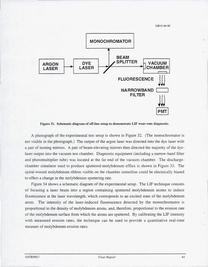
C9012 -04-99

MONOCHROMATOR

~

BEAM

ARGON DYE / SPLITTER 0 VACUUM .... .. .. CHAMBER LASER LASER / .r--1

FLUORESCENCE JD NA RROWBA NO IL....-----I

FILlER

Figure 31. Schematic diagram of off-line setup to demonstrate LIF wear-rate diagnostic.

A photograph of the experimental test setup is shown in Figure 32. (The monochromator is

not visible in the photograph. ) The output of the argon laser was directed into the dye laser with

a pair of turning mirrors. A pair of beam-elevating mirrors then directed the majority of the dye

laser output into the vacuum test chamber. Diagnostic equipment (including a narrow-band filter

and photomultiplier tube) was located at the far end of the vacuum chamber. The discharge

chamber simulator used to produce sputtered-molybdenum efflux is shown in Figure 33. The

spiral-wound molybdenum ribbon visible on the chamber centerline could be electrically biased

to effect a change in the molybdenum sputtering rate.

Figure 34 shows a schematic diagram of the experimental setup. The LIF technique consists

of focusing a laser beam into a region containing sputtered molybdenum atoms to induce

fluorescence at the laser wavelength, which corresponds to an excited state of the molybdenum

atom. The intensity of the laser-induced fluorescence detected by the monochromator is

proportional to the density of molybdenum atoms, and, therefore, proportional to the erosion rate

of the molybdenum surface from which the atoms are sputtered. By calibrating the LIF intensity

with measured erosion rates, the technique can be used to provide a quantitative real-time

measure of molybdenum erosion rates.

94FR9967 F illa/ Report 44

, I

~ .. ' .

ARGON LASER

, .. ~ .. ~ ~ ~, ' . ". ,- -',=.. '.: . '-

"' , 't • •

.:: .. . .: - .......... --.. -...... - .... ~.

VVINDO'l.' ./

/",/

. i · .'

2' VACUUf,,1 CHAMBER

'\

Figure 32. Photograph of experimental setup for investigating LIF wear-rate diagnostic.


19267

BEAM STOP

9C 1 2·C~ · i CC

Figure 33. Photograph of discharge-chamber simulator for demonstrating LIF wear-rate diagnostic.


_._- - ---

LIF RADIATION

MONOCHROMATOR

--_L --------- . ----r

I J

QUARTZ WINDOWS ---r:::::::i~

i LASER BEAM

C9012-15-71R5

LASER BEAM STOP

COILED Mo FOIL

XENON "---....--.-__ ~_ GAS

FLOW

SIMULATOR DISCHARGE CHAMBER

Figure 34. Schematic of LIF test setup.

A 30-cm-diam discharge-chamber simulator was used to provide a source of xenon ions for

sputtering. The surface to be sputtered consisted of a spiral-wound coil of thin (O.OOS-mm)

molybdenum foil that was electrically isolated and mounted at the 8-cm-diam exit aperture of the

discharge-chamber simulator, as shown in Figure 34. With this arrangement, the sputtering rate

of the molybdenum foil could be controlled by biasing it electrically, without affecting the

plasma conditions within the discharge chamber.

A Spex Model l700-II monochromator was used to measure the intensity of the laser

induced-fluorescence radiation, with a wavelength resolution of a few tenths of an Angstrom. A

lens with a 60-cm focal length focused the radiation into the monochromator. The focal length

of this lens was chosen to provide a close match to the f-number of the monochromator, in order

to fill the grating and obtain the best possible resolution for a given setting of the entrance and

exit slits. The output of the monochromator was fed into a photomultiplier tube.

The total signal detected by the monochromator consists of laser-induced fluorescence (LIF),

plasma-induced fluorescence (PIF), and scattered laser light. Several features were incorporated

into the vacuum chamber shown in Figure 34 to reduce the background signal arising from

scattered laser light and plasma-induced fluorescence of the molybdenum atoms. An optically


black beam-stop (fabricated from quartz tubing coated with black soot from an acetylene torch)

was installed to minimize scattered laser light. Two metal apertures were used to limit the

background radiation produced by the discharge-chamber simulator. The first aperture. located

I8-cm downstream of the molybdenum coil, is a rectangular slot I8-cm-wide by I .3-cm-high.

with the long dimension placed in the plane of the laser beam. The second aperture, (located

66-cm downstream of the molybdenum foil,) has a IO-cm-diam aperture. which is the same

diameter as the quartz window located at the entrance slit of the monochromator.

In order to use the LIF technique to induce and detect fluorescence of sputtered molybdenum

atoms, the output from the dye laser was set to a wavelength corresponding to the desired

molybdenum resonance (A = 390.2 nm). Frequency selection was accomplished with an

intracavity birefringent tuning element, which also limited the laser bandwidth to about

300 GHz. The laser-output power was approximately 70 mW. The laser beam was amplitude

modulated with a chopper at a frequency of 1 kHz, producing a modulated LIF signal at the same

frequency (in contrast to the relatively constant level of the plasma-induced background). A

lock-in amplifier was used to eliminate the dc background due to plasma-induced fluorescence.

Both the dc-coupled output from the photomultiplier tube of the monochromator and the output

from the lock-in amplifier were observed simultaneously on a dual-trace oscilloscope.

We demonstrated the LIF technique with the discharge-chamber simulator operated at a

discharge voltage of VD = 27 V and a cathode-emission current of JE = 18 A. Figure 35 shows

the LIF signal (top trace) and the total photomultiplier output (bottom trace) for the case where

no bias voltage was applied to the molybdenum foil to enhance its sputtering rate. Note that the

dc photomultiplier signal (lower trace) remains essentially zero, while the scattered laser light is

observable in the top trace.

Figure 36 shows the effect of increasing the bias voltage of the molybdenum foil to enhance

its sputtering rate. Figure 36(a) shows that the LIF signal increases by about a factor of 1.5 times

the background level (which is caused by scattered laser light and previously shown in

Figure 35) at a bias voltage of VB = 70 V. As expected, the plasma-induced fluorescence signal

increases as well. Figure 36(b) shows that increasing the bias voltage to VB = 150 V results in

an LIF signal that is a factor-of-two greater than the background level.


. I

o LEVEL LlF SIGNAL

o LEVEL PIF SIGNAL

JE = 18 A VD = 27 V

VSIAS = 0 V

9312·04· 102

LlF SIGNAL, 1.0 VlDiv PIF SIGNAL, 0.5 V/Div

Figure 35. Laser-ioduced-fluorescence (LIF) and plasma-induced-fluorescence (PIF) signals at A = 390.2 om. Standard plasma conditions and with no bias voltage applied to the Mo foil.

We varied the plasma conditions by increasing both the discharge voltage (to VD = 29 V) and

cathode-emission current (to JE = 20 A) to provide a higher flux of higher energy xenon ions for

sputtering the molybdenum foil. Figure 37 shows that for a bias voltage of VB = 150 V, the LIF

signal is increased by nearly a factor-of-four over the background signal shown in Figure 32 (the

oscilloscope sensitivity was reduced by a factor-of-two in Figure 37).

The results of Figures 35 to 37 demonstrated that the LIF technique can be used to detect

sputtered molybdenum. For all of the measurements we obtained, the output level from the lock

in amplifier due to the LIF was on the order of Volts . A high signal-to-noise ratio was confirmed

by blocking the laser beam at the entrance to the vacuum chamber and noting that there was no

discernible background signal produced by the lock-in amplifier. The frequency jitter of the

laser was large enough to cause its output to drift through the molybdenum resonance,


o LEVEL LlF SIGNAL

o LEVEL PIF SIGNAL

o LEVEL LlF SIGNAL

o LEVEL PIF SIGNAL

JE = 18 A Vo = 27 V

VSIAS = 70 V

(8) 70-V BIAS

JE = 18 A Vo = 27 V

VBIAS = 150 V

(b) 150-V BIAS

4-.

9312-04-1 0:;

LlF SIGNAL, 1.0 VlDiv PIF SIGNAL, 0.5 VlDiv

LlF SIGNAL, 1.0 VlDiv PIF SIGNAL, 0.5 VlDiv

Figure 36_ LIF and PIF signals at A = 390.2 nm_ Standard plasma conditions and with bias voltage applied 10 the Mojoil.


o LEVEL LlF SIGNAL

o LEVEL PIF SIGNAL

JE = 20 A Vo = 29 V

VS1AS = 150 V

9312·0': · 10.:

LlF SIGNAL, 1.0 V/Div PIF SIGNAL, 0.5 V/Div

Figure 37. LIF and PIF signals at A = 390.2 nm. Enhanced-sputtering plasma conditions and with 150· V bias vo/rage applied to the Mo foil.

which is probably in the range of lOs of GHz (recall that the laser bandwidth is about 300 GHz),

resulting in a fairly noisy LIF signal (even after lock-in detection). The data shown in Figures 35

to 37 were taken with the integration time of the lock-in amplifier set at 3 s. Even at this setting

there was a slow (on the order of seconds) drift in the LIF signal, while the dc-coupled output of

the photomultiplier remained unchanged. This behavior suggests that drift of the laser frequency

is probably the cause of the amplitude drift that we observed. A set of etalons (for UV operation)

within the dye-laser cavity were eventually used to reduce its output to a single longitudinal

mode with a jitter on the order of 20 MHz. Since this jitter is roughly three orders of magnitude

smaller than the width of the molybdenum resonance, a steady LIF output could be achieved.

We explored whether the LIF signal levels detected in this manner have long-term stability

and repeatability under conditions that maintained constant discharge-plasma parameters

(constant molybdenum sputtering rate) . In addition, we explored the sensitivity of the detected

LIF signals to changes in molybdenum erosion rates. Using the experimental setup shown in

Figure 34, we observed relatively large-amplitude fluctuations (frequency of approximately 10 to

100 Hz) on the apparent LIF signal, which was dependent on the bias voltage applied to the

molybdenum foil. We had to use very long (30 to 100 s) integration times on the lock-in

amplifier in order to "smooth out" these fluctuations and obtain a stable LIF signaL We

attributed the apparent LIF fluctuations to the large PIF signal sensed by the monochromator.


We modified the design of the molybdenum foil to minimize the PIF signal (and the random

noise fluctuations it produces), and to maximize the LIF signal. Figure 38(a) shows the coiled

molybdenum foil originally used to demonstrate the LIF wear-diagnostic technique, but which

allows the PIF signal to reach the monochromator. Figure 38(b) shows a modified molybdenum

foil design that uses louvers instead of a coil. This improved design also increases the

molybdenum surface area, yielding a higher density of sputtered material. The louvered-foil

arrangement reduces the PIF signal reaching the monochromator, while increasing the magnitude

of the LIF signal. With the louvered-foil arrangement, we verified that the random-noise

fluctuations present in the apparent LIF signal were significantly reduced and that the PIF signal

was also reduced (by an order of magnitude). We were able to lower the integration time of the

lock-in amplifier to 3 s, obtaining stable and repeatable LIF signals.

LENS

LASER BEAM STeP

-1 t J ~~ON I_~FLOW

J LASER BEAM

SIMll.ATOR DISCHARGE CHAMBER

(a) SETUP W ITH COILED Mo FOIL

"~~'~~~ )~ = = 1 " J ~:::~ / , I l / I_~ FLOW

I SIMll.ATOR LENS ~ DISCHARGE

I CHAMBER OUARTZ WIN DOW S '

J LASER BEAM

(b) SETUP WITH LOUVERED Mo BAFFLE

Figure 38. Use of louvered baffie (b) to improve LIF signal strength over the coil (a ).

We varied the bias voltage applied to the molybdenum foil and recorded the LIF signal on a

strip-chart recorder. Figure 39 shows the temporal behavior of a representative LIF signal , along

with various electrical parameters of the discharge-chamber simulator, and the laser-output

power. The operating parameters of the discharge-chamber simulator (cathode-emission current,

discharge voltage, and cathode flow rate) were maintained constant in order to achieve constant

plasma conditions. As shown in Figure 39, the LIF signal is relatively constant over time


9312-04-075 -5V tint = 3 sec

~ -OV - 5V

I PLASER I - 0 V ·0.5 A

I J S1AS I I I · 0 V

·200 V

~ I 1

150V

I'OOV l50v l,v ·ov ·10 SCCM

G:J .,scJ ·50 V

[ ~

·0 V ·25 A

t ~ · 0 A

t=O t (min) 40 min

Figure 39. Strip-chart recording of LIF signal, discharge-chamber parameters, and laser-output power.


for fixed bias voltage. As the bias voltage is lowered (to reduce the molybdenum erosion rate),

the LIF signal level is reduced as well. indicating that changes in the molybdenum density can

indeed be detected (cf., Figure 39 and Figure 40) . Decreasing the bias voltage also reduced the

random-noise fluctuations, whereas blocking the laser-beam input at full-bias-voltage conditions

had little effect on the fluctuations. This indicates that the random-noise fluctuations on the

apparent LIF signal are primarily induced by the plasma. Note that the discharge voltage stays

constant, unaffected by changes in bias voltage, so that the changes in molybdenum sputtering

rate are due solely to the change in bias voltage.

94FR9967

28-7226-04

5 r----------------------------,

4

-> -3 -J < Z

" ~ 2 -..J

1

o~------------~------------~ o 100 200 Mo FOIL BIAS VOLTAGE (V)

Figure 40. LIF test setup and experimental results.

Filial Report 54

4.3 THRUSTER MEASUREMENTS

We adapted the laser and monochromator setup shown in Figures 38(a) and 38(b) for

demonstrating that LIF could be used to detect molybdenum sputtered from the negative

electrode of an operating thruster. Figure 41 shows a schematic diagram of the setup that was

used to accomplish this in our 9-ft-diam vacuum chamber. Mirrors were used to direct the laser

beam to the top port of the vacuum chamber. The laser beam entered the chamber through a

quartz window and traversed the ion beam as indicated in Figure 41. A beam stop located on the

vacuum-chamber floor minimized reflection of the laser light within the vacuum chamber. A

light-absorbing collimator, which extends from the side port into the vacuum chamber

approximately 46 em, minimized the contribution of reflected laser light to the background LIF

signal.

CRYOPUMP

QUARTZ LASER , _ WINDOW BEAM ', - - '- -,'

II II

(TOP PORT) ----....~~p-====~~L<..~-~--~--~-=~~~:J ~~;!=@~=f

LlF RADIATION COLLIMATOR

QUARTZ ------0 WINDOW (SIDE PORT) MONOCHROMATOR

DIFFUSION PUMP

Figure 41. Schematic of "on-line" LIF setup.

9112-04-21

LIF radiation produced by the laser beam interacting with sputtered molybdenum in the ion

beam was detected using a 3/4-m monochromator, which is positioned at the side port of the

9-ft-diam vacuum chamber (see Figure 42). In this location, the monochromator viewed the ion

beam orthogonal to the laser beam, and without any interference caused by radiation from the

discharge-chamber plasma.


\0 -I>. 'T1 ~ \0 \0 (J\ -.J

~ is -~ {l C)

4

VI (J\

.- ~~.

r.' ~ -~" I' I '\;;-'JiO;"~;~,~~~ i t . . .... /, ~ . . ~ , \ •. ! , ~q

-<'- J-- - ~ '< , . ' " I' ,.'-0 , '~I· ~~~i?~ . . ..,.. __ ~ , - , ~ '~"''' 1 I I , " ,._ ...............

.................... a::.:.t " "}\~"· t'

.---- ... -.. " .... .

, '. i' Iii.". '" ., I I ' , . SEA

..... ..... y' I LA .. '.~,l, ..... ..... " .~. ". .............. .,'\,

..... .......... ~~ ,-...... -~r..., ,,.

.... (t;' MONOCHROMATOR

,( !

Figure 42. Experimental setup for demonstrating LlF as a diagnostic for measuring accelerator-grid wear.

.~- --- -.----.- .. -----~~ .... -.-.---~ .. _-- -~ ----

The output beam of an argon-ion-pumped, standing-wave dye laser was directed through the

top port of our 9-ft-diam vacuum chamber using an arrangement of mirrors . The fluorescence

signal produced as the light beam passes through molybdenum atoms (which have been sputtered

from the accel grid of the thruster under test) was detected by the monochromator. Figure 43

(which was taken from the open end of our 9-ft-diam vacuum chamber) shows the top port and

collimator through which the laser beam enters the chamber. A light dump and collimator

located in the bottom of the chamber absorbed the laser beam. A collimator that minimizes

scattered light from reaching the monochromator is visible in the right of the photo. A movable

molybdenum plate served as a reflector to allow laser light, or plasma-induced fluorescence from

within the discharge chamber, to reach the monochromator for calibration purposes. The

molybdenum plate also served as a strong source of sputtered material, which was used for

adjusting both the laser frequency and the monochromator wavelength. The experimental

arrangement shown in Figure 43 was found necessary to yield LIF data with good signal-to-noise

ratio.

Figure 44 shows LIF-signal measurements (the output of the photomultiplier tube in the

monochromator was divided by the measured laser-output power, which drifts slightly) as a

function of accelerator-electrode current for two different accelerator voltages. The accel current

was increased by introducing xenon into the vacuum chamber from an auxiliary gas source. The

LIF signal exhibits the anticipated dependence on acce! current (sputtering rate), and the relative

increase in the LIF signal with acce! voltage is consistent with an increase in sputter yield at

higher energy.

Figure 45 shows the LIF signal as a function of accelerator voltage for three different acce!

currents , with the current variation produced by introducing xenon into the vacuum chamber.

The trends are consistent with the dependence of sputtering rate on current density and the

dependence of sputter yield on ion energy.

To gain additional physical insight from the data shown in Figure 45, we plotted the variation

of sputter yield with accelerator voltage in Figure 46 for one of the curves from Figure 45. The

data indicate that the LIF signal and the sputter yield have that same functional dependence on

accelerator voltage. The preliminary results of Figures 44, 45, and 46, are believed to

adequately demonstrate the validity of LIF as a real-time diagnostic for assessing relative

accelerator-grid wear rates in ion thrusters . We believe absolute wear rates could be obtained by

calibrating the LIF signal using measured wear rates.


--------- --- ... _---

Figure 43. LIF setup in HRL's 9-ft-diam vacuum chamber.


931 2-04-077

1.0

Vb = 1200 V

- V A = -600 V en 0.8 t: Jb = 3.0 A z :::> (rlrnd)unc = 0.71 > a: « 0.6 a: .... £Xl

Vb = 1500 V a: « VA = -350 V - 0.4 ..J « Jb = 3.0 A z G (l1rnd)unc = 0.81 en u. 0.2 ..J

o .o~ ______ ~ ________ ~ ______ ~ ________ ~ ______ ~ 20 30 40 50 60 70

ACCEL CURRENT (rnA)

Figure 44. Variation of LIF signal with accelerator current.


9312-04-076

2.0 JA = 69 rnA

Po = 6x10-5Torr~ - Jb = 3.0 A en I-

1.5 Vb = 1200 V z => (11 rnd>unc= 0.52 > a: <%: a: I-m 1.0 a: <%: -...J Z <%: ~ JA = 60 rnA en 0.5

Po = 4.6x10-5Torr u.. ...J

o.o~ ______ ~ ______ ~ ________ ~ ______ ~ ______ ~ 200 300 400 500 600 700

ACCEL VOLTAGE (V)

Figure 45. Variation of LIF signal with accelerator voltage.


---- --

,--

9112-15-248R1

OJ 1 .6~----T-----~----~----~----~~--~

rz 1.4 => >- 1.2 a: « a: 1.0 r-~ 0.8

=:s 0.6 ~ « z 0.4 C)

en 0.2

VB = 1200 V (Tlmd)unc = 52%

JA = 60 rnA

Po = 1.6x10-5 Torr

1.4 --c o

1.2 ~ E

1.0 B co -->-0.8 o ~

0.6 UJ

0.4

0.2

>a: UJ

~ O~----~----~----~--~~--~~--~ 0

rr=> 0.. en

1 00 200 300 400 500 600 700

ACCEL VOLTAGE, VA (V)

Figure 46. Comparison of LIF signal level and sputter yield behavior as a function of accelerator voltage level.


Section 5 LAMINAR-THIN-FILM EROSION BADGES

5.1 BADGE CALIBRATION

We calibrated laminar-thin-film (LTF) erosion badges with bulk molybdenum, using the

calibration setup shown in Figure 47. For each test, a small piece of perforated L TF badge

material was placed adjacent to a piece of polished molybdenum (arc-cast, low carbon content).

The LTF badge was partially masked using a stainless-steel strip, and the bulk-molybdenum

sample was masked in several locations using photoresist material. The samples were exposed to

sputtering beams of 300-e V Xe+, Kr+, and Ar+ for a duration sufficient to remove several of the

molybdenum layers on the L TF badges. After the beam exposure, the L TF mask was removed to

permit the number of sputtered layers to be counted. The photoresist mask was removed from

the bulk-molybdenum sample to permit the erosion depth to be measured using a surface

profilometer. This calibration was repeated on at least one additional set of samples to establish

the level of uncertainty in the LTF measurement technique.

e9012·04·98

PHOTO-

Figure 47. Schematic illustra ting technique for calibrating LTF erosion badge with bulk Mo.


After exposing the samples to a monoenergetic flux of the test ions for a specified period of

time, the samples were removed for diagnostic analysis . The LTF badges were examined under

a microscope to determine the number of molybdenum layers that had been removed through ion

sputtering, and this determination was subsequently confirmed by performing a diagnostic etch

to reveal the remaining layers. In determining the total erosion depth, the eu layers were treated

as equivalent, partial-thickness layers of the 600-A-thick molybdenum layers. The fractional

layer thickness, k, was calculated as k = (Y MolY Cu)(nCu/nMo), where Y is the sputter yield and n

is the number density. For 300-eV Ar+ and Xe+, the numerical value of the fractional layer

thickness was determined to be k = 0.45, based on published sputter yields and material

densities . In other words , the copper layers were treated as equivalent molybdenum layers

having a reduced thickness of 0.45 x 600 = 270 A. The bulk-molybdenum erosion rates were determined by chemically removing the

photoresist mask and then measuring the surface features with a profilometer. Figure 48 shows a

typical measurement result, displaying flat peaks and valleys of relatively uniform height.

9312-04-078

10 10

9

J 9 ~ I' \

--"\ 8 V 8

7 7

6 l 6

5 5 '----( 4 4

3 3 SAMPLEAR-2

2 GRATING ETCH INTO BULK Mo 2 3680 A ,

1

I I I I 1 -r

SCALE: 1000 A o o

Figure 48_ Surface-profilometer measurement of sputter-etch pattern on bulk-Mo calibration sample.


Calibration results are shown in Figure 49, with the bulk-molybdenum results plotted versus

the LTF results, and with perfect correlation indicated by the straight line. The uncertainties in

the measurement techniques are indicated by the error bars , where we used 250- and 600-A as

the uncertainty in the direct-measurement and layer-counting technique, respectively. Although

most of the calibration data fall on, or near, the straight line, some of the results (particularly the

data obtained with Xe+) depart from perfect correlation by more than the indicated error bars.

9412-04-087

5000

o 300-eV Argon

D 300-eV Xen on 0« 4000

I 0 300-eV Krypton f-0.. W 0

~ z 3000 0 (f)

0 cr: w 0 2000 :2 , ~ -.J :::) CD

1000

O ~--------~----------~----------~--------~----------~ o 1 000 2000 3000 4000 5000

L TF EROSION DEPTH, A

Figure 49. Bulk-Mo vs. LTF erosion-rate results for 300-eV Ar+, Kr+, and Xe+ ions.

5.2 THRUSTER TEST

We conducted a short-term (:::::} h) test to measure the erosion rate of the accel and screen

electrodes of our 30-cm-diam lab-model thruster using LTF erosion badges. The intent was to

correlate these results with those obtained during the 900-hr test conducted at NASA - LeRC. A

six-hour badge test was estimated to be sufficient to provide measurable erosion rates , based on

the aceel current and voltage measured during the LeRC test.

Erosion badges having dimensions of approximately 13-mm by 13-mm were spot-welded to

the downstream surface of the accel electrode and the upstream surface of the screen electrode.


Figures 50 and 51 are photographs showing the locations of the badges on the accel and screen

grids, respectively. A total of eight LTF badges were mounted on the accel grid and two LTF

badges were mounted on the screen grid.

We operated the 30-cm-diam lab-model thruster at conditions that closely simulate those

representative of the LeRC life test. Table 8 compares the critical thruster and facility conditions

of our short-term test with those of the LeRC test. The accel current and voltage are the most

critical parameters to match in order to simulate the same charge-exchange-ion erosion

conditions of the acce! electrode. Table 8 indicates that all thruster parameters were duplicated

except for the discharge voltage, which was adjusted to achieve the desired accel current at the

indicated vacuum-chamber pressure.

Figure 52 shows photographs of the erosion badges after removal from the accel electrode .

The badge that was mounted at the 314-radius location is not included in the photo because it had

not been eroded enough to expose a copper line. The photographs clearly show the copper-line

patterns resulting from charge-exchange-ion erosion of the webbing between apertures of the

acce! electrode. The erosion rates were determined from these patterns by counting the number

of copper lines remaining after the exposure.

Figure 53 is a plot of the LTF-badge wear rates obtained from analyzing the photographs at

the "triangular-pit" regions where the erosion rates are the highest. For comparison, results of

the accel-electrode erosion measured at the completion of LeRC's 900-h life test are also

presented. The results presented in Figure 53 indicate that the erosion-badge wear rate has a

peaked profile. There is also good agreement between the LTF-badge results and the LeRC life

test results , at least for the centerline location.

The peaked behavior of the erosion-badge wear rates is consistent with operation of the

thruster at high propellant-utilization efficiency. For the ring-cusp thruster, the ion-production

region (and, therefore, the ion-beam profile) becomes increasingly peaked on centerline as the

propellant-utilization efficiency is increased. The charge-exchange-ion production rate is

directly proportional to the product of ion-beam density and neutral density. Assuming a

constant neutral density across the diameter of the ion beam, the charge-exchange-ion erosion

profile is expected to have very nearly the same peaked profile as the ion-beam-density profile.

Table 11 compares the operating conditions during the erosion-badge test with those of the

900-h life test. Although the beam current, lb, acce! voltage, V A, discharge voltage, VD, and

discharge propellant-utilization efficiency, (llmd)unc, were matched to the NASA-LeRC life test

values , the accel current in the erosion-badge test was about 40% higher than it was in the life

test. The duration of the erosion-badge test was 1 hour, which was sufficient to allow erosion

patterns to be visible on the badges, but without eroding through all the layers.


=

Figure 50. LTF erosion-badge installation on accel grid.

Figure 51. LTF erosion-badge installation on screen grid.


(a)

6 Cu LINES VISIBLE

(b)

3 Cu LINES VISIBLE

(c)

1 Cu LINE VISIBLE

Figure 52. Photos of L TF erosion badges.


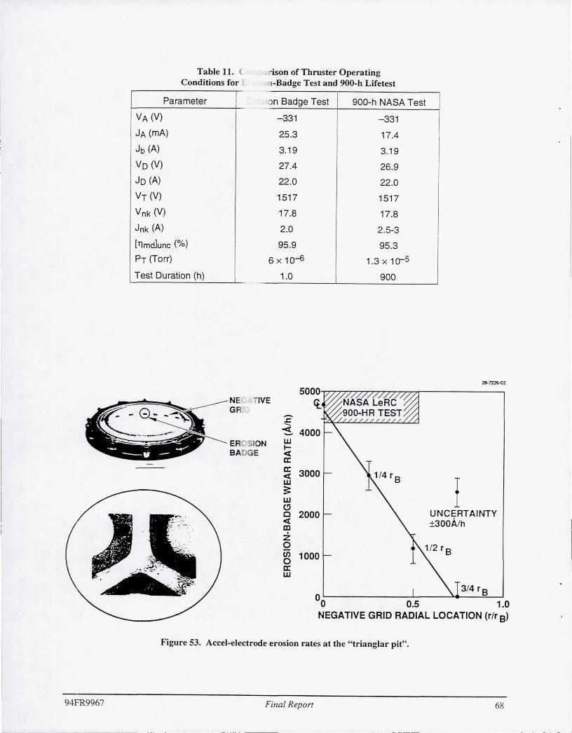
94FR9967

Table 11. ( Conditions for

Parameter

VA (V)

JA (mA)

Jb (A)

VD (V)

JD (A)

VT (V)

Vnk (V)

Jnk (A)

[llmd]unc (%)

PT (Torr)

Test Duration (h)

ison of Thruster Operating -Badge Test and 900-h Lifetest

n Badge Test 900-h NASA Test

-331 - 331

25.3 17.4

3.19 3.1 9

27 .4 26.9

22.0 22.0

1517 1517

17.8 17.8

2.0 2.5-3

95.9 95.3

6 x 10-6 1.3 x 10-5

1.0 900

5000~n77/rn~/T~7r-----------' NE IVE ct. G

ER SION BADGE

-.l:: ~ 4000 w ~ ct a: ~ 3000 w ;: w C,!) o 2000 ct m Z o ~ 1000 a: w

I UNCERTAINTY ±30oA/h

3/4 rB OL-------------~----~~--~~ o 0.5 1.0 NEGATIVE GRID RADIAL LOCATION (r/r B)

Figure 53. Accel-electrode erosion rates at the " t r ianglar pit".

Filial Report 68

. I

I '

..... _--- . ... __ ._--_._ .... _ --- --_ ... _ ---_ .... _._- -_ ... _'-

Section 6 FACILITY EFFECTS

6.1 PUMPING SPEED MEASUREMENTS

We evaluated the pumping speed of the Hughes vacuum chamber for the inert gases xenon.

krypton, and argon. Figure 54 shows chamber pressure measured at the location indicated in

Figure 1 (obtained by subtracting the baseline pressure of about 2.5x 1 0-7 Torr from the indicated

pressure and dividing the result by the ionization-gauge sensitivity for xenon of 2.5) as a function

of flow rate expressed in Torr-liters/s. Both the chamber pressure and flow rate were measured

using instruments that were calibrated in the Hughes Primary Standards Laboratory against

reference values that are traceable to NBS standards. Our flow meters are calibrated on xenon.

and our ionization gauge is calibrated on N2. The highly repeatable data shown in Figure 54

were obtained on separate occasions (four days apart).

9312-04-082 10r----------------------------------------,

12 {? --6

fD o

)(

w ex: ::::> en ffi 4 ex: c.

2

o FIRST MEASUREMENT

o REPEAT MEASUREMENT

0.5 1 1.5 2

FLOW RATE (Torr-Iiters/s)

Figure 54. Vacuum-chamber pressure as a function of xenon flow rate, showing repeatability of measurements taken several days apart.


We used the flow-meter constants9 listed in Table 12 to convert the indicated readings when

testing with krypton and argon gases , (i.e. , we multiplied the indicated readings by the factor

1.4311.37 to convert to argon flow rates). The indicated pressures were converted to the

appropriate gas pressures by subtracting the baseline pressure (typically 2x 10-7 to 3x 10-7 Torr)

and dividing the result by the appropriate ionization-gauge sensitivity. 10 The ionization-gauge

sensitivities listed in Table 12 were obtained by averaging the values tabulated in the manual for

our ionization-gauge controller. 1 0

Table 12. Instrument Sensitivities

Gas Flow Meter Constant Ion Gauge Sensitivity

Xenon 1.37 2.50

Krypton ' 1.39 1.77

Argon 1.43 1.12

Figures 55 to 57 present pressure vs . flow rate for the three test gases , showing a high degree

of linearity. The pumping speeds obtained from the slope of these curves are listed in Table 13,

showing the expected increase in pumping speed realized with the lighter gases.

9412·04-085

10 .-----------~------------~----------~--~--------,

XENON GAS

8

'E' ~ (0

. 6 0 ~

x ill a: :::> (f)

4 (f) w a: a.

2

OLr------------~------------~----------~------------~ o 0 .5 1.0 1.5 2.0

FLOW RATE, (Torr-l iters's)

Figure 55. Curve fit of chamber pressure vs. Xe flow rate; reciprocal of the slope establishes pumping speed as 135,000 Iiters/s.


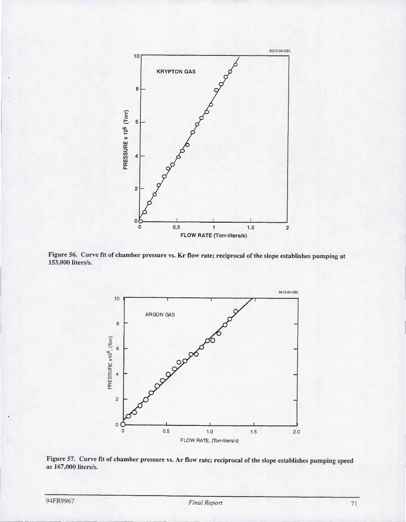
9312·04·083

10

KRYPTON GAS

8

... 0 t:. 6

'" 0

)(

w a: => !Jl 4 !Jl W a: c.

2

o~--------~------~--------~--------~ o 0.5 1.5 2

FLOW RATE (Torr-litersls)

Figure 56. Curve fit of chamber pressure vs. Kr flow rate; reciprocal of the slope establishes pumping at 153,000 liters/so

9412-04-086

10

ARGON GAS

8

~ 6 <0 0

X

W cr => (J) 4 (J) w H:

2

OLr----------~----------~----------~----------J o 0.5 1.0 1.5 2.0

FLOW RATE. (Torr-litersls)

Figure 57. Curve fit of chamber pressure vs. Ar flow rate; reciprocal of the slope establishes pumping speed as 167,000 liters/s.


-- ... _---

Table 13. Measured Pumping Speeds

Gas Pumping Speed (liters/s) I !

Xenon 135,000

Krypton 153,000

Argon 167,000

Figure 58 shows "normalized pumping speed" (obtained by multiplying the measured

pumping speed by the square root of the atomic mass number) plotted versus the mass number.

If the pumping speed were controlled by free-molecular flow to the cryotub inlets, then the

normalized pumping speed is given by the expression S = (8kT/n:)1/2A/4, where T is the

chamber-wall temperature and A is the effective pumping area. In Figure 58 , we have

normalized the theoretical value to coincide with the measured value for xenon . (The

normalization is equivalent to assuming that the effective pumping area of our cryotubs is about

59% of their geometrical open area.) We normalized the results to xenon because it has the

lowest vapor pressure of the three gases (argon has the highest). The reason for the departure of

krypton and argon from the theoretical normalized pumping speed is not known ; since the

departure is greatest for argon, one can speculate that it may be due to the vapor-pressure effect.

Ion gauge sensitivities for argon, for example, have been reported to vary by as much as 25%,

depending on the gauge, and this could also contribute to a large uncertainty in pumping speed.

9412-04'()84

2 .0e+06

~ (J)

III 1.8e+06 -ci w w

THEORETICAL VALUE a. CJ)

1.6e+06 CJ z 0:: ~ =:l a. 0 1.4e+06 w N :::i « ~ a: 1.2e+06 0 z

1.0e+06 0 50 100 150

MASS NUMBER

Figure 58. Normalized pumping speed obtained for Xe, Kr, and Ar compared with theoretical value.


6.2 FACILITY-PRESSURE EFFECTS

We evaluated the effect of facility pressure on the accelerator-electrode current of our 30-cm

diam lab-model thruster equipped with ion optics SIN 917 geometry summarized in Table 14.

Xenon was introduced into the vacuum chamber through a leak valve, while adjusting the

thruster flow rates to maintain the discharge propellant utilization constant. Figure 59 shows the

resultant variation in acce! current for two different values of discharge voltage.

We explored the effect of facility pressure on accelerator-electrode current, taking advantage

of the increased pumping speed (achieved by installing two additional 1.2-m-diam cryotubes) of

our 9-ft-diam vacuum chamber to explore a facility-pressure regime that was previously

unattainable at Hughes. Figure 60 shows the variation of accel current with vacuum-chamber

pressure for the 8-cm thruster SIN 907 operated on xenon. For these tests, the increase in facility

pressure was achieved by introducing xenon directly into the vacuum chamber from an auxiliary

supply tank.

When the acce! current is plotted versus the log of chamber pressure, as in Figure 60. the

accel-current behavior changes from one that appears to be relatively independent of chamber

pressure (neutral-loss-rate dominated) to one that is strongly dep~ndent on chamber pressure

(facility dominated).

Figure 61 compares the variation of acce! current with facility pressure for the 30-cm lab

model thruster operated at a beam current of J b = 3.2 A. For both curves of Figure 61 , the

discharge voltage and the discharge propellant-utilization efficiency are constant. For thruster

operation at a beam current of Jb = 3.2 A, the acce! current appears to be facility dominated, even

at the minimum (baseline) facility pressure that we could achieve.

The data presented in Figure 62 were obtained in our 9-ft-diam vacuum chamber with the

increased pumping capability that was described earlier. Figure 62 compares the variation in

acce! current with facility pressure before and after the facility was modified, showing the

dramatic reduction in accel current that is realized under the lower pressure conditions of the

modified facility . Although the increased pumping speed of our upgraded test facility results in

nearly a factor-of-three reduction in accel current, the accel current at the baseline pressure still

appears to be facility dominated at this level of beam current.

Table 14. Summary of SIN 917 Grid Parameters.

Parameter I Screen Grid I Accel Grid

Aperture Diameter, mm I 1.91 1.14 I I

Thickness, mm I 0.25 0.38 I I

Hole Spacing, mm I 2.20 2.21

Open Area, % ! 67.8 24.3

Aperture Geometry I Round Round


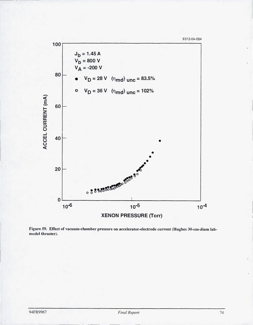
9312-04-084

100

Jb = 1.45A

Vb = 800 V

V A = -200 V

80 f-Vo = 28 V (T1md) unc = 83.5% •

0 Vo = 36 V (T1md) unc = 102% -c=: E - 60 f-~ Z W a: a: => u ...J W 40 f-U • U c=:

• • • 20 f--

~. ~o

~ .~~~,

00

0 I

10-6 10-5 10-4

XENON PRESSURE (Torr)

Figure 59. Effect of vacuum-chamber pressure on accelerator-electrode current (Hughes 30-cm-diam labmodel thruster).


9312-04-085

0.8

Jb = 72 rnA

Vb = 1200 V

V A = -300 V

0.6

-<t E -I-Z • W • c:: 0.4 • c:: • :::J (.) • ...J • W • U .... (.) •• <t ... •• • • •

0.2 I I I

NEUTRAL LOSS RATE FACILITY DOMINATED DOMINATED

o~--------------------~--------------------~ 10-7 10-6 10-5

FACILITY PRESSURE (Torr)

Figure 60_ Effect of vacuum-chamber pressure on accel current (8-cm-diam thruster SIN 907).

, .


-~ E -IZ W a: a: ::::> (J

..J W U U ~

9312-04-087

100

Vo = 28 V

80

Jb = 3.2 A

(llmd) unc = 97% 60

o

o o

40

20

o~----------------------~--------------------~ 10-6 10-5 10-4


Figure 61- Effect of beam current on accel-currentlchamber-pressure relationship. (Hughes 30-cm-diam lab-model thruster)

94FR9967 Filial Report

• I

76

-~ E -~ Z W c: c: ::> ()

...J W () () ~

9312-04-088

100~--------------------------------------~

80 '-

60 I--

40 I--

20 -

• OLD PUMPING FACILITY

o NEW PUMPING FACILITY

VD = 28 V

•• •• •

•• •••

• • • . ~ •

• • • •

• Jb = 3.22 A

• • (T) md)unc = 93%

• • •

·0 · 0 Jb = 3.2 A

o (T)md)unc = 97%

O~--------------------I~------------------~ 10-6 10-5 10-4

XENON PRESSURE (torr)

Figure 62. Dramatic redution in accel current achieved through modifications to improve the pumping speed of Hughes 9-ft·diam vacuum chamber.


We also operated the 30-cm-diam lab-model thruster at the same conditions as the NASA

LeRC life-test thruster, in order to obtain data for comparing facility effects in the NASA and

Hughes test chambers. Figure 63 shows the variation of accel current with facility pressure at a

beam current of Jb = 3.2 A. This operating condition was selected from the NASA-LeRC life

test results . For comparison, Figure 69 also includes the results presented in Figure 67 for

thruster operation at a higher discharge voltage (higher propellant-utilization efficiency). The

lack of an effect of neutral loss rate in the data of Figure 63 is consistent with the notion that the

accel current is dominated by facility effects.

Additional insight into the facility-pressure effect is apparent when the accel

current/chamber-pressure data are plotted on a linear graph. For example, replotting the data of

Figure 60 in this manner results in Figure 64, which reveals two very linear regimes separated by

an abrupt change in slopes. The first linear regime (at low facility pressure) corresponds to what

was previously referred to as the neutral-loss-rate-dominated behavior of the acce! current. in

which the acce! current is only weakly dependent on facility pressure. The second linear regime

shown in Figure 64 corresponds to what was previously referred to as the facility-dominated

behavior of the accel current, in which the acce! current is strongly dependent on facility

pressure.

Figure 65 shows the same dual-slope linear behavior of the acce! current with facility

pressure for the 30-cm-diam lab-model thruster operated at a beam current of Jb = 1.45 A.

Extrapolating the low-pressure segments of the curves to zero facility pressure results in acce!

currents of 3 to 4 rnA, or approximately 0.2 to 0.3 % of the beam current. This low percentage is

consistent with our experience with the J-series mercury thruster, which operates with an accel

current fraction of about 0.2% at vacuum-chamber pressures in the low 10-6 Torr range.

Figure 66 shows the data of Figure 65, along with a linear-linear replot of data from

Figure 61. For the higher beam current, the accel current appears linear over the entire range of

facility pressure. There is no "break" in the curve, consistent with the notion that the accel

current is facility dominated, even at the lowest facility pressure.

Insight into the behavior of the acce! current with facility pressure evident in Figures 62 to 64

can be gained by reviewing the various contributions to the total acce! current, J A,

(2)

where Jlh is the acce! current in the absence of facility pressure, and 1r is the acce! current due to

the facility pressure. The contribution Jlh is from the neutral loss rate. For constant discharge

94FR9967 Filla! Report

9312-04-089

100 • Vo = 27 V

Vb= 1516 V

V A = -338 V

(llmd)unc = 97% 80 r- Ei = 11geVlion .. 125 eVlion

0 Vo = 28 V

- Vb= 1500 V « E V A = -300 V - 60 -.... (llmd)unc = 93% z

~ w Ej = 126 eV/ion .. 130 eV/ion 0: 0: 0 ::J • (,) 0 ..J C)

w 4Q - 0 (,) ,pI (,) «

/ Jb = 3.2 A 20 I--

O~--------------------I~------------------~ 10-6 10-5 10-4


Figure 63. Effect of discharge voltage on accel-currentlchamber-pressure relationship.


l_.

-~ E -~ z w c: c: ::::> u ...J w u u ~

1.0

0.8

0.6

0.4-

0.2

Jb = 72 rnA

Vb = 1200 V V A = -300 V

9312-04-093

o~------------------~------------~--------~--------~--------~--------~ o 0.2 0.4 0.6 0.8 1.0 1.2 1.4

XENON PRESSURE x 105 (Torr)

Figure 64. Effect of vacuum-chamber pressure on accel current (8-cm thruster SIN 907).

94FR9967 Fillal Repon 80_~ ---~

1-

30

25

- 20 <t E -.Z w a: a: 15 :::J ()

...J W () () <t 10

Jb = 1.45 A Vb = 800 V

VA = -200 V

5 / /

/

• Vo = 36 V

(llmd)unc ::::: 102%

o Vo = 28 V

(llmd)un-c ::::: 83.5%

9312-04-091

o~----~------~------~----~------~----~ o 0.5 1.0 1.5 2.0 2.5 3.0


Figure 65. Effect of discharge voltage on accel-currentlchamber-pressure relationship.


-<t E -I-z w a: a: => u --' w U U <t

94FR9967

9312-04-092 60~--------------------------------------------'

50

40

30

20

Jb = 1.45 A

Vo = 36 V

10

Jb = 3.2 A

Vo = 28 V

Jb = 1.45 A

Vo = 28 V

O~------~------------~------~------_I~----~ o 0.5 1.0 1.5 2.0 2 .5 3.0

XENON PRESSURE x 105 (torr)

Figure 66. Effect of beam current on accel-currenUchamber-pressure relationship.

Fillal Report 82

--- -----.--- ------~ --'- ._--- --~-.--- .. ~~ ._- --

propellant-utilization efficiency, the neutral loss rate is a constant, and, therefore, Jth is also a

constant. The facility contribution to the acceI current, Jr. is assumed to be independent of J tho

and to depend only on the density of gas in the facility , which is directly proportional to the

facility pressure, p. Equation (2) can therefore be rewritten as,

JA=A+Bp, (3)

where A and B are constants. Equation (3) predicts a linear dependence of accel current on

facility pressure_ The intercept should be nearly equal to the space-environment accel current

that would be realized in the absence of facility pressure.

The results presented in Figures 64 to 66 verify the linear dependence predicted by

Equation (3), however they show a dual linear behavior that is not predicted. The accel-current

intercept for the low-pressure data shown in Figure 65 is very close to the value expected on the

basis of the accel current being approximately 0.2% of the beam current in the absence of a

facility effect. This is consistent with what has been recorded for J-series thrusters operating on

mercury propellant, where the facility effect is minimaL The encouraging aspect of the

characteristics shown in Figure 66 is that the highly linear nature of the results would permit a

confident extrapolation of the accel current to the limit of zero facility pressure, as long as the

facility pressure is low enough to establish the "break" in the characteristic .

Figure 67 shows the variation of the acceI current with chamber pressure for the 8-cm-diam

lAPS thruster operated on xenon. We documented the behavior of the beam-plasma potential of

the 8-cm-diam thruster for two extreme chamber-pressure conditions (1.4x 10-7 Torr and 4xlO-6

Torr). As can be seen from the data presented in Figure 67, the low-pressure value minimizes

the facility contribution to the acceI current, while the high-pressure value maximizes the facility

effect on acce1 current.

6.3 BEAM-POTENTIAL MEASUREMENTS

We measured the probe floating profile by sweeping a hot-filament probe through the beam

in the manner described in the final report2 for Phase 1_ Figure 68 shows a schematic of the

filament-probe assembly. To determine the filament current for performing the plasma-potential

measurements, we measured the variation of beam potential with filament current with the probe

positioned at the beam centerline and outside the beam edge_ Figure 69 compares the variation

of the beam potential with filament current (filament temperature) when the probe is in and out

of the beam_ The data indicate that a filament current of 4.3 A is sufficient to achieve operation

in the plateau region of the probe characteristic for both locations of the probe. The hot filament

probes when located in the neutralized beam should float new plasma potential.


-ct E -t-z w a: a: ::J U ...I w u u ct

- -- - - - - - - - -

9312-04-090

1.0r------------------------------------------------.

0.8

0.6

0.4

0.2

Jb = 72 rnA

Vb = 1200 V

V A = -300 V

o~----~----~------~----~----~----~----~ o 0.2 0.4 0.6 0.8 1.0 1.2 1.4


Figure 67. Variation of accel-grid current with vacuum-chamber pressure (8-cm thruster SIN 907).

94FR9967 Filla! Report

. . -- -----

84

94FR9967

/

TUNGSTEN FILAMENT

9312-04-094

TANTALUM SUPPORT RODS

DOUBLE-BARREL ALUMINA TUBE

STAINLESS-STEEL TUBE SHIELD

Figure 68. Sketch showing filament-type beam probe.

Filial Repon 8S

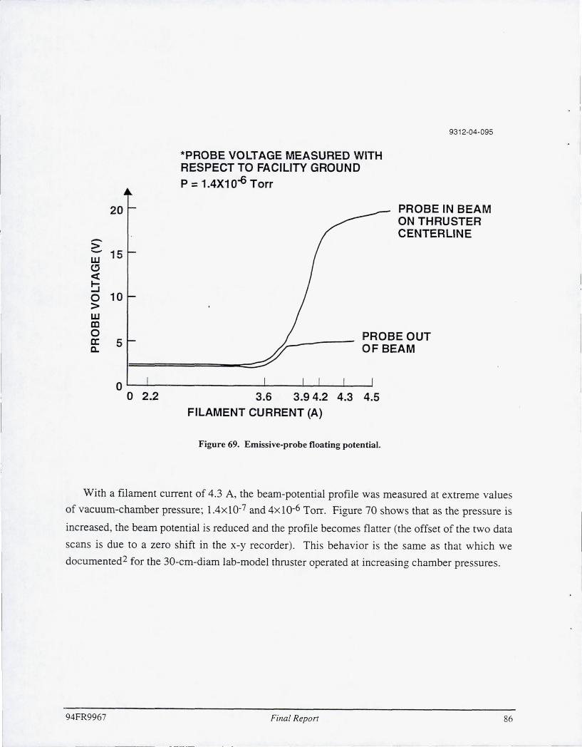
20

> - 15 w (!) <t ~ o 10 > W al o a: 5 Q.

*PROBE VOLTAGE MEASURED WITH RESPECT TO FACILITY GROUND P = 1.4X10-6 Torr

9312-04-095

PROBE IN BEAM ON THRUSTER CENTERLINE

PROBE OUT OF BEAM

O~~----------------~----~--~--~~

o 2.2 3.6 3 .9 4.2 4.3 4.5 FILAMENT CURRENT (A)

Figure 69. Emissive-probe floati ng potential.

With a filament current of 4.3 A, the beam-potential profile was measured at extreme values

of vacuum-chamber pressure; 1.4xlO-7 and 4x lO-6 Torr. Figure 70 shows that as the pressure is

increased, the beam potential is reduced and the profile becomes flatter (the offset of the two data

scans is due to a zero shift in the x-y recorder). This behavior is the same as that which we

documented2 for the 30-cm-diam lab-model thruster operated at increasing chamber pressures.


--- .. _--

• I

r-I

94FR9967

9312-04-096

FILAMENT CURRENT = 4.3 A

20 P = 1.4X1 0-7 Torr

> -.-oJ 15 ~ ~ z ~ 10 ~ P = 4X10-6 Torr w m 5 o L--------------------------a: a..

o ~------------------------------------------~ 40°

PROBE LOCATION (DEGREES)

Figure 70. Effect of vacuum·chamber pressure on probe floating potential variation.

Filial Repon 87

Section 7 REFERENCES

1. 1.R. Beattie and J.N. Matossian, "Mercury ion thruster technology," Final Report, Hughes Research Laboratories, NASA CR-174974, Mar 1989.

2. J .R. Beattie and J.N. Matossian, "High power ion thruster technology," Final Report, Hughes Research Laboratories, NASA CR-187161 , Feb 1992.

3. M.S. Patterson and T.R. Garver-Verbey, 21st International Electric Propulsion Conference, Orlando, Florida, AlA A Paper 90-658, July (1990).

4. B.A. Rock, M.A. Mantenieks, and M.L. Parsons, 18th International Electric Propulsion Conference AIAA Paper 85-2011 , Alexandria, VA (1985).

5. J.M. Stone, Radiation and Optics (McGraw-Hill, New York, 1963).

6. A. Yariv, Quantum Electronics, 2nd ed. (Wiley, New York, 1975).

7. M. Kaminsky, Atomic and Ionic Impact Phenomena on Metal Surfaces (Academic, New York, 1965).

8. KG. Whitney and J. Davis, J. Appl. Phys. 45, 5294 (1974).

9. Teledyne Hastings-Raydist, "Instruction manual for Hastings mass flowmeter," C 194D, 1974.

10. Varian Vacuum Products Division, "Manual for Model 880RS digital ionization gauge controller," Appendix B, 1987. (From NASA Technical Note TND-5285).

11. J.M. Monheiser, "Development and Verification of a Model to Predict Impingdment Currents for Ion Thruster," NASA CR-195322, Colorado State University, April 1994.


----------- ---- ----

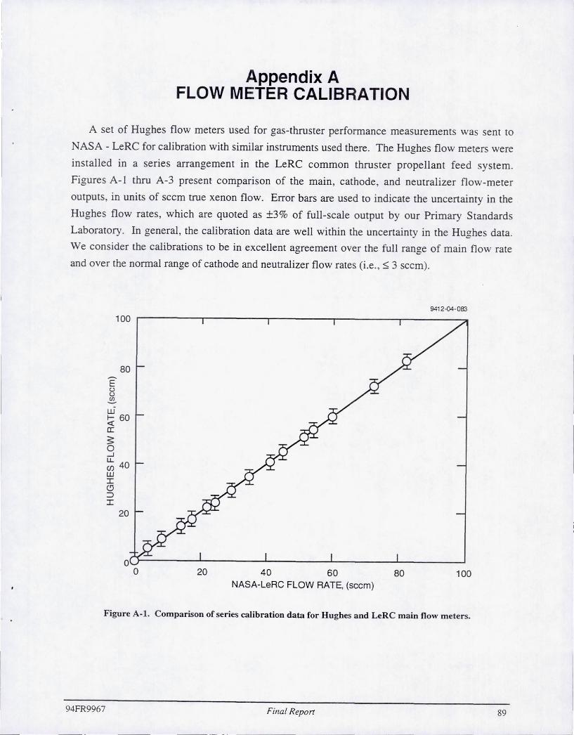
Appendix A FLOW METER CALIBRATION

A set of Hughes flow meters used for gas-thruster performance measurements was sent to

NASA - LeRC for calibration with similar instruments used there. The Hughes flow meters were

installed in a series arrangement in the LeRC common thruster propellant feed system.

Figures A-I thru A-3 present comparison of the main, cathode, and neutralizer flow-meter

outputs , in units of sccm true xenon flow. Error bars are used to indicate the uncertainty in the

Hughes flow rates, which are quoted as ±3% of full -scale output by our Primary Standards

Laboratory. In general, the calibration data are well within the uncertainty in the Hughes data.

We consider the calibrations to be in excellent agreement over the full range of main flow rate

and over the normal range of cathode and neutralizer flow rates (i.e., ~ 3 sccm).

100

E C,.) C,.)

.!!l.-w

80

t- 60 ~ a: ~ o -l

LL 40 en w I (9 ~ I

20

o o

9412·04· 083

20 40 60 80 100 NASA-LeRC FLOW RATE, (seem)

Figure A-I. Comparison of series calibration data for Hughes and LeRC main flow meters.


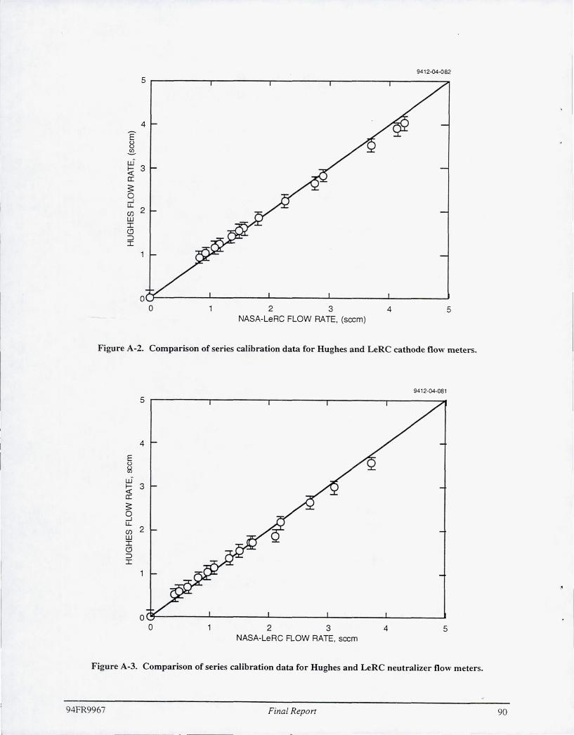
9412-04-082

5 ~--------~---------.----------r---------.---------~

4

E 8

.!:E.-w

3 ~ a:: ~ 0 ....J U.

2 Cf) w I 0 :;) I

2 3 4 5 NASA-LeRC FLOW RATE, (seem)

Figure A-2_ Comparison of series calibration data for Hughes and LeRC cathode flow meters_

9412-04-081

4

E ()

&l L.Li f- 3 ~ ~ 0 ....J U. Cf) 2 w I 0 :;) I

NASA-LeRC FLOW RATE, seem

Figure A-3_ Comparison of series calibration data for Hughes and LeRC neutralizer flow meters_


J

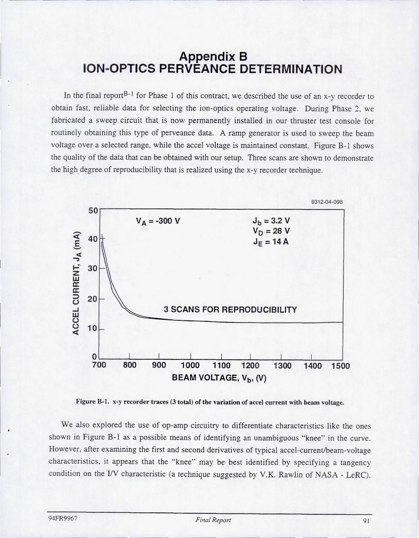
Appendix B ION-OPTICS PERVEANCE DETERMINATION

In the final reportB- 1 for Phase 1 of this contract, we described the use of an x-y recorder to

obtain fast , reliable data for selecting the ion-optics operating voltage . During Phase 2, we

fabricated a sweep circuit that is now permanently installed in our thruster test console for

routinely obtaining this type of perveance data. A ramp generator is used to sweep the beam

voltage over a selected range, while the accel voltage is maintained constant. Figure B-1 shows

the quality of the data that can be obtained with our setup. Three scans are shown to demonstrate

the high, degree of reproducibility that is realized using the x-y recorder technique.

9312-04-098

50r---------------------------------------------.

~ 40 E -c:t .., .... ~ 30 z w a: a: ;:) 20 ()

...J W ()

() 10 ~

VA = -300 V J b = 3.2 V Vo = 28 V JE = 14A

3 SCANS FOR REPRODUCIBILITY

O~ ____ ~ ____ ~ ____ ~ ____ ~ ____ ~ ____ ~ ____ ~ ____ ~ 700 800 900 1000 1100 1200 1300 1400 1500

BEAM VOLTAGE, Vb, (V)

Figure B-l. x-y recorder traces (3 total) of the variation of accel current with beam voltage.

We also explored the use of op-amp circuitry to differentiate characteristics like the ones

shown in Figure B-1 as a possible means of identifying an unambiguous "knee" in the curve.

However, after examining the first and second derivatives of typical accel-currentlbeam-voltage

characteristics, it appears that the "knee" may be best identified by specifying a tangency

condition on the VV characteristic (a technique suggested by V.K. Rawlin of NASA - LeRC).


For example, Figure B-2 shows tangents drawn to a typical characteristic having slopes of

-0.067, -0.1 , and -0.133 rnA/V (-30, -45, and -60°, respectively for these scales). Although the

selection of the "best" slope to define the knee is arbitrary, the results of Table B-1 show that the

location of the knee is not too sensitive to the value of lhe slope used to define it. Therefore, we

adopted a value of -0.1 rnA/Vas the slope of the tangent to be used in defining the knee of the

curve. It appears that a conservative specification of the minimum operating voltage can then be

achieved by adding 200 V to the knee value.

-« E -<t J

....... z w a: a: ::::> ()

..J w () ()

«

94FR9967

9312-<J4-099 50

Jb = 1.45 A

Vb = 800 V

40 V A = -200 A

dJA dVb

30

d2JA

dVb2 20

10

45° TANGENT LINE O~ ____ ~I _______ I~ ____ ~I ______ ~ ______ ~I ______ ~ 500 600 700 800 900 1000 1100

BEAM VOLTAGE, Vb, (V)

Figure B-2. Tangents used to define "knee" condition.

Table B-l. Beam Voltage Obtained from Knee of Curves in Figure 10.

Slope (mNV) Voltage (V)

-0.067 625

-0.100 610

-0.133 595

Filla/ Repon 92

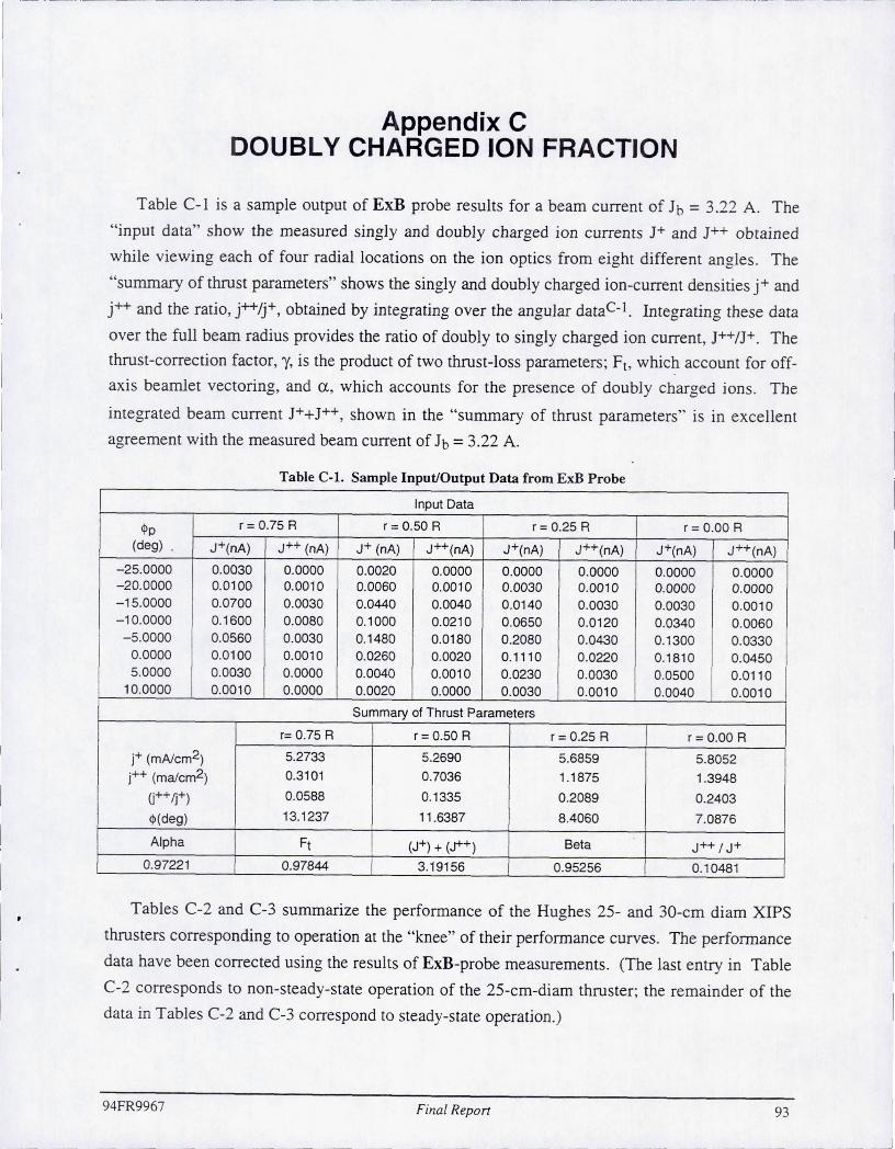
I'-~-'-'

I

I

I

I ·

)

--- --~---~'--- '- ----'--~'-

Appendix C DOUBLY CHARGED ION FRACTION

Table C-l is a sample output of ExB probe results for a beam current of Jb = 3.22 A. The

"input data" show the measured singly and doubly charged ion currents J+ and J++ obtained

while viewing each of four radial locations on the ion optics from eight different angles. The

"summary of thrust parameters" shows the singly and doubly charged ion-current densities j + and

j++ and the ratio, j++jj+, obtained by integrating over the angular dataC-1. Integrating these data

over the full beam radius provides the ratio of doubly to singly charged ion current, J++jJ+. The

thrust-correction factor, y, is the product of two thrust-loss parameters; F£, which account for off

axis beamlet vectoring, and a., which accounts for the presence of doubly Charged ions. The

integrated beam current J++J++, shown in the "summary of thrust parameters" is in excellent

agreement with the measured beam current of Jb = 3.22 A.

Table C-l. Sample Input/Output Data from ExB Probe

Input Data

<pp r = 0.75 R r = 0.50 R r= 0.25 R r = 0.00 R

(deg) J+(nA) J++ (nA) J+ (nA) J++(nA) J+(nA) J++(nA) J+(nA) J++(nA)

-25.0000 0.0030 0.0000 0.0020 0.0000 0.0000 0.0000 0.0000 0.0000 -20.0000 0.0100 0.0010 0.0060 0.0010 0.0030 0.0010 0.0000 0.0000 -15.0000 0.0700 0.0030 0.0440 0.0040 0.0140 0.0030 0.0030 0.0010 - 10.0000 0. 1600 0.0080 0.1000 0.0210 0.0650 0.0120 0.0340 0.0060 -5.0000 0.0560 0.0030 0.1480 0.0180 0.2080 0.0430 0.1300 0.0330

0.0000 0.0100 0.0010 0.0260 0.0020 0.1110 0.0220 0.1810 0.0450 5.0000 0.0030 0.0000 0.0040 0.0010 0.0230 0.0030 0.0500 0.0110

10.0000 0.0010 0.0000 0.0020 0.0000 0.0030 0.0010 0.0040 0.0010

Summary of Thrust Parameters

r= 0.75 R r = 0.50 R r = 0.25 R r = 0.00 R

j+ (mAlcm2) 5.2733 5.2690 5.6859 5.8052

j++ (ma/cm2) 0.3101 0.7036 1.1875 1.3948

U++/j+) 0.0588 0.1335 0.2089 0.2403

<p(deg) 13.1237 11 .6387 8.4060 7.0876

Alpha Ft (J+) + (J++) Beta J++ / J+

0.97221 0.97844 3.1 9156 0.95256 0.1 0481

Tables C-2 and C-3 summarize the performance of the Hughes 25- and 30-cm diam XIPS

thrusters corresponding to operation at the "knee" of their performance curves. The performance

data have been corrected using the results of ExB-probe measurements. (The last entry in Table

C-2 corresponds to non-steady-state operation of the 25-cm-diam thruster; the remainder of the

data in Tables C-2 and C-3 correspond to steady-state operation.)


- - - -------1

Table C-l. 25-cm-diam XIPS Thruster Performance

Jb £i Po Pb PT 11e F Isp 11md 11mt TIt (A) (W/A) (W) (kW) (kW) y2 (%) (mN) (s) (%) (%) (%)

1.45 120 173 1.6 1.8 .94 86.7 77 3188 85.2 80.7 66

3.22 124 398 4.7 5.3 .91 89.8 195 4224 98.2 93.2 76

4.0 120 477 6.2 6.8 .89 90.3 245 4338 99.5 94.6 76

*5.0 126 606 8.2 9.1 .89 90.5 316 4795 105.8 101.3 82

"Extrapolated from 1.45, 3.22, and 4.0 beam-current data for 0 excessive equilibrium temperature at Jb=5 A did not

permit ExB measrement.

Table C-3. 30-cm-diam XIPS Thruster Performance

Jb £i Po Pb Pr 11e F Isp 11md 11mt 11t (A) (W/A) (W) (kW) (kW) 1- (%) (mN) (s) (%) (%) (%)

1.45 121 125 1.2 1.4 .97 83 66 2330 78 69 55

3.22 120 386 3.5 4.0 .90 87 158 3226 93 88 69

3.22 120 387 4.7 5.1 .91 91 193 4200 97 94 77

4.0 120 480 5.0 5.6 .89 88 208 3676 98 94 74

5.0 125 626 9.0 9.8 .89 92 330 5025 104 102 83

*5.6 140 785 10.0 11 .1 .87 90 364 5160 108 106 83

"No ExB data were measured because of overheating of ExB probe at the high form level. The d is extrapolated for plasma currents.

I

I

Figure C-l shows the variation of integrated doubly to singly charged ion-current ratio J+/1++

with discharge propellant-utilization efficiency. As anticipated, there is an increase in the doubly

charged ion fraction with discharge propellant-utilization efficiency. At 90% efficiency,

approximately 9% of the beam current is doubly charged. Figure C-2 shows the centerline value

of the doubly to singly charged ion-current density ratio j++jj+ for the 30-cm-diam thruster. At a

discharge-propellant-utilization of 90%, the doubly charged current fraction on centerline is

about 25%.


-- ---- - -_ .. -- ----

I . \

\

\

\

\

\

I

\

I

I

I

I i

· I

1-

Jb = 1.45 A 25-cm

Input Data ! I

~p r = 0.75 R r = 0.50 R r = 0.25 R r = 0.00 R I (deg) J+(nA) J++ (nA) J+ (nA) J++(nA) J+(nA) J++(nA) J+(nA) i J++(nA)

-20.0000 0.0300 0.0000 0.0100 0.0000 0.0100 0.0000 i

0.0100 I 0.0000 , I

-15.0000 0.0200 0.0100 0.0200 0.0000 0.0100 0.0000 0.0100

I 0.0000 I

-10.0000 0.0300 0.0150 0.2100 0.0200 0.0400 0.0000 0.0150 0.0000 -5.0000 0.3100 0.0150 0.3800 0.0350 0.2600 0.0300 0.0800 0.0100

0.0000 0.2100 0.0100 0.3500 0.0300 0.4000 0.0450 0.3000 0.0300 5.0000 0.0300 0.0000 0.2000 0.0150 0.3400 0.0300 0.4100 0.0450

10.0000 0.0150 0.0000 0.0200 0.0000 0.1700 0.0150 0.3200 0.0350


r= 0.75 R r = 0.50 R r = 0.25 R r = 0.00 R

j+ (mAlcm2) 2.4074 2.3630 2.3490 3.6813

j++ (malcm2) 0.1120 0.1918 0.2309 0.2941

U++/j+) 0.0465 0.0812 0.0983 0.0799

<p(deg) 10.8694 7.2152 7.4412 14.6030

Alpha Ft (J+) + (J++) Amps Beta J++ / J+

0.98254 0.98595 1.19768 0.97019 0.06340

Jb = 3.22 A 25-cm

Input Data

<pp r= 0.75 R r = 0.50 R r = 0.25 R r = 0.00 R


-20.0000 0.0000 0.0000 0.0000 0.0000 0.0000 0.0000 0.0000 0.0000 -15.0000 0.0400 0.0050 0.0150 0.0000 0.0000 0.0000 0.0000 0.0000 -10.0000 0.0700 0.0150 0.0650 0.0100 0.0150 0.0000 0.0050 0.0000

-5.0000 0.0600 0.0050 0.1200 0.0200 0.0700 0.0200 0.0350 0.0100 0.0000 0.0250 0.0000 0.0600 0.0100 0.1150 0.0300 0.1000 0.0300 5.0000 0.0050 0.0000 0.0400 0.0000 0.0800 0.0200 0.1200 0.0300

10.0000 0.0050 0.0000 0.0400 0.0000 0.0800 0.0200 0.1 200 0.0300 15.0000 0.0000 0.0000 0.0000 0.0000 0.0300 0.0100 0.0650 0.0200


r= 0.75 R r= 0.50 R r = 0.25 R r = 0.00 R

j+ (mAlcm2) 4.7947 9.2098 10.0144 10.3419

j++ (malcm2) 0.2776 0.5244 2.6413 3.1029

U++/j+) 0.0579 0.0569 0.2637 0.3000

<j>(deg) 9.8952 9.0810 9.8584 8.5191

Alpha Ft (J+) + (J++) Amps Beta J++ / J+

0.96902 0.98595 3.53249 0.94712 0.11827


$p r = 0.75 R

(deg) J+(nA) J++ (nA)

-20.0000 0.0050 0.0000 -1 5.0000 0.0400 0.0050 -10.0000 0.0800 0.0100 -5.0000 0.1000 0.0100

0.0000 0.0500 0.0050

5.0000 0.0100 0.0000

10.0000 0.0000 0.0000

r= 0.75 R

j+ (mAlcm2) 5.7565

j++ (malcm2) 0.5960

U++jj+) 0.1035

$(deg) 10.6784

Alpha Ft

0.95671 0.98690

$p r=0.75R


-20.0000 0.0120 0.0000 -15.0000 0.1150 0.0000 -10.0000 0.3330 0.0150 -5.0000 0.1170 0.0010

0.0000 0.0150 0.0000 5.0000 0.0000 0.0000

10.0000 0.0000 0.0000

r= 0.75 R

j+ (mAlcm2) 0.7269

j++ (malcm2) 0.0002

U++jt) 0.0003

$(deg) 9.8739

Alpha Ft

0.99481 0.98923

94FR9967

Jb = 4.0 A 2S-cm

Input Data

r = 0.50 R r = 0.25 R

J+ (nA) J++(nA) J+(nA) J++(nA)

0.0020 0.0000 0.0000 0.0000 0.0150 0.0020 0.0000 0.0000 0.0800 0.0150 0.0220 0.0050 0.1400 0.0300 0.0600 0.0200 0.1000 0.0200 0.1500 0.0500 0.0600 0.0100 0.1200 0.0400 0.0150 0.0000 0.0500 0.0200


r = 0.50 R r = 0.25 R

8.7030 7.4761

1.4718 2.5646

0.1691 0.3430

7.5573 7.7786

(J+) + (J++) Amps Beta

3.69919 0.92609

Jb = 1.45A 30-cm

Input Data

r = 0.50 R r = 0.25 R


0.0000 0.0000 0.0000 0.0000 0.0820 0.0030 0.0080 0.0000 0.4330 0.0180 0.0830 0.0070 0.4060 0.0110 0.6390 0.0200 0.0550 0.0000 0.4000 0.0130 0.0020 0.0000 0.0520 0.0000 0.0000 0.0000 0.0020 0.0000


r = 0.50 R r = 0.25 R

1.2799 1.4110

0.0383 0.0497

0.0299 0.0352

8.7740 4.9447


0.53419 0.99114

Filial Report

r = 0.00 R

J+(nA) I J++(nA)

0.0000 0.0000 0.0000 0.0000 0.0050 0.0000 0.0200 0.0050 0.0800 0.0300 0.1600 0.0600 0.1200 0.0400

r = 0.00 R

7.9468

2.2742

0.2862

8.2015

J++jJ+

0.17345

r= 0.00 R

J+(nA) J++(nA)

0.0000 0.0000 0.0000 0.0000 0.0370 0.0000 0.2680 0.0210 0.7380 0.0380 0.1460 0.0020 0.0290 0.0000

r = 0.00 R

1.4202

0.0687

0.0483

5.8880

J++jJ+

0.01804

96

I

. \

\

- - - --- _.- -.~-.---.-- .-... --. -~

I~-

<pp r = 0.75 R


-20.0000 0.0150 0.0000 -15.0000 0.1000 0.0100 -10.0000 0.1500 0.0100

-5.0000 0.0550 0.0050 0.0000 0.0150 0.0000 5.0000 0.0000 0.0000

10.0000 0.0000 0.0000

r= 0.75 R

j+ (mAlcm2) 5.7282

j++ (ma/cm2) 0.4479

U++/j+) 0.0782

<p(deg) 11.0589

Alpha Ft

0.96459 0.98461

<pp r = 0.75 R


-20.0000 0.0200 0.0000 -15. 0000 0.0900 0.Q1 00 -10.0000 0.1000 0.0100

-5.0000 0.0500 0.0000 0.0000 0.0100 0.0000 5.0000 0.0000 0.0000

10.0000 0.0000 0.0000

r= 0.75 R

j+ (mAlcm2) 4.9397

j++ (ma/cm2) 0.3069

r .

U++/j+) 0.0621

cp(deg) 12.0287

Alpha Ft

0.96953 0.98363

94FR9967

Jb = 3.22A 30-cm Vb =3.5kW

Input Data

r= 0.50 R r = 0.25 R

J+ (nA) J++(nA) J+(nA)

0.0000 0.0000 0.0000 0.0500 0.0100 0.0200 0.1800 0.0200 0.0700 0.1400 0.0150 0.2100 0.0400 0.0000 0.1200 0.0000 0.0000 0.0300 0.0000 0.0000 0.0000


r = 0.50 R

6.1425

0.6706

0.1092

8.3818

(J+) + (J++) Amps

3.78820

Jb = 3.22A 30-cm Pb =4.7kW

Input Data

J++(nA)

0.0000 0.0100 0.0200 0.0450 0.0250 0.0100 0.0000

r = 0.25 R

7.5574

2.2572

0.2987

9.0331

Beta

0.93956

r = 0.50 R r = 0.25 R


0.0100 0.0000 0.0050 0.0000 0.0600 0.0100 0.Q150 0.0000 0.1700 0.0300 0.0700 0.0200 0.1300 0.0200 0.2100 0.0650 0.0300 0.0000 0.1200 0.0300 0.0100 0.0000 0.0400 0.0100 0.0000 0.0000 0.0100 0.0000


r = 0.50 R r = 0.25 R

6.9753 8.4008

0.7901 1.8123

0.1133 0.2157

8.8134 8.4409


3.63068 0.93956

Final Report

r= 0.00 R

J+(nA) I J++(nA)

0.0000

I 0.0000

0.0100 0.0000 0.0400 0.0100 0.1400 0.0400 0.2000 0.0500 0.0700 0.0200 0.0000 0.0000

r = 0.00 R

7.5202

1.7939

0.2385

7.7935

J++ / J+

0.13751

r = 0.00 R

J+(nA) J++(nA)

0.0000 0.0000 0.Q1 00 0.0000 0.0350 0.0100 0.1400 0.0450 0.2300 0.0750 0.0800 0.0200 0.0200 0.0000

r = 0.00 R

7.7274

1.9953

0.2582

7.6397

J++ / J+

0.11609

97 I I

~I

Jb =4 A 30-cm

Input Data

<p p r= 0.75 R r = 0.50 R r= 0.25 R r = 0.00 R


-20.0000 0.0150 0.0000 0.0100 0.0000 0.0100 0.0000 0.0000 0.0000 I -1 5.0000 0.0800 0.0100 0.0500 0.0150 0.0250 0.0100 0.0000 0.0000

-10.0000 0.1900 0.0200 0.1900 0.0300 0.0800 0.0200 0.0400 0.0150

-5.0000 0.0600 0.0100 0.1500 0.0200 0.2300 0.0600 · 0.1400 0.0500

0.0000 0.0200 0.0000 0.0400 0.0100 0.1300 0.0300 0.2000 0.0700

5.0000 0.0100 0.0000 0.0100 0.0000 0.0400 0.0100 0.0700 0.0300

10.0000 0.0000 0.0000 0.0000 0.0000 0.0100 0.0000 0.0300 0.0100


r= 0.75 R r = 0.50 R r = 0.25 R r = 0.00 R

j+ (mNcm2) 5.8558 7.2448 9.7576 6.6902

j++ (ma/cm2) 0.5607 1.3340 2.5097 2.5755

U++jj+) 0.0958 0.1841 0.2572 0.3850

<p (deg) 9.1080 8.4121 9.7763 6.3228

Alpha Ft (J+) + (j++) Amps Beta J++ j J+

0.95978 0.98722 4.31250 0.93134 0.1591 7

Jb = 5 A 30-cm

Input Data

<pp r= 0.75 R r = 0.50 R r = 0.25 R r = 0.00 R

(de g) J+(nA) J++ (nA) J+ (nA) J++(nA) J+(nA) J++(nA) J+(nA) J++(nA)

- 20.0000 0.0200 0.0000 0.0100 0.0000 0.0000 0.0000 0.0000 0.0000 - 15.0000 0.1100 0.0100 0.0700 0.0150 0.0200 0.0100 0.0150 0.0100 - 10.0000 0.1900 0.0200 0.2800 0.0550 0.0900 0.0300 0.0400 0.0150 -5.0000 0.0600 0.0100 0.2000 0.0350 0.3200 0.1300 0.1800 0.0800

0.0000 0.0200 0.0000 0.0500 0.0100 0.1800 0.0600 0.3100 0.1600 5.0000 0.0000 0.0000 0.0150 0.0000 0.0350 0.0100 0.0900 0.0300

10.0000 0.0000 0.0000 0.0000 0.0000 0.0100 0.0000 0.0200 0.0000


r= 0.75 R r = 0.50 R r = 0.25 R r = 0.00 R

j+ (mNcm2) 6.5542 10.2004 10.0754 9.7242

j++ (ma/cm2) 0.5645 1.6836 3.7818 4.4770

0++ f]+) 0.0861 0.1650 0.3753 0.4604 1 \

<p (deg) 10.6708 8.0840 8.7721 8.4473

Alpha Ft (J+) + (J++) Amps Beta J++ j J+

0.95570 0.98613 5.06932 0.92437 0.17822


-- -~- ------' L .~ ________ _

- .- - - - - - -~ _._-- -

I ~-- - - - - - - - -

I

I

I ·

I .

I

I

I

I

r

I

I

I

r

I

I f

I

0.30 VD = 28 V

o 30 em THRUSTER

0.25 - • 25 em THRUSTER

+ 0.20-~ + + .., o i= <t 0.15-a: .... z w a: a: a 0.10-

0.05 -

9312-04-100

o~------~--------~--------~-------+------~

60 70 80 90 100 110

DISCHARGE PROPELLANT-UTILIZATION EFFICIENCY, (llmd)une

Figure C-l. Variation of doubly to singly charged ion-current ratio with measured discharge propellantutilization efficiency.


J

I

I I

l I

l

0.6

0.5 -

+ 0.4-:::::::-+ + '-~ o i= c:x: II: ~ Z W II: II: ::> U

0.3 -

0.2 -

0.1 -

9312-04-101

VD = 28 V

o 3.22 A

o~------~--------~--------~-------+------~

60 70 80 90 100 110

DISCHARGE PROPELLANT-UTILIZATION EFFICIENCY,

(llmd)unc (%)

Figure C-2. Variation of doubly to singly charged ion-current density ratio with measured discharge propellant-utilization efficiency.


I . \

1 \

- - --!

,- - - - - '- - - - - - - '-- -- - - - - - - - - - -- -- -- -- 1

I <

I

r

Appendix D APPENDICES REFERENCES

B-1 J.R. Beattie and J.N. Matosian, "High Power Ion Thruster Technology," Final Report. Hughes Research Laboratories, NASA CR-187161, Feb. 1992.

C-l J.R. Beattie, "Extended Performance Technology Study: 30-cm Thruster, " Final Report. Hughes Research Laboratoies, NASA CR-168259, June 1983.


NJ\S/\ Report Documentation Page National Aeronautics and Space Administration

1. Report No. 2 . Government Accession No. 3. Recipient's Catalog No.

NASA CR-195477

4. Title and Subtitle 5. Report Date

High-Power Ion Thruster Technology June 1996

6. Periorming Organization Code

7. Author(s) 8. Periorming Organization Report No.

l.R. Beattie and J.N. Matossian E-9693

10. Work Unit No.

9. Periorming Organization Name and Address

Hughes Research Laboratories 11 . Contract or Grant No. 301 1 Malibu Canyon Road NAS3-25553 Malibu, CA 90265

13. Type of Report and Period Covered 12. Sponsoring Agency Name and Address

Final 10/20/89 - 10/20/92 Lewis Research Center 21000 Brookpark Road 14. Sponsoring Agency Code

Cleveland, OH 44135

15. Supplementary Not~s Project Manager: James S. Sovey

NASA Lewis Research Center. Cleveland. OH 44135 J216) 977-7454 16. Abstract

Performance data are presented for the NASAlHughes 30-cm-diam "common" thruster operated over the power range from 600 W to 4.6 kW. At the 4.6-kW power level, the thruster produces 172 mN of thrust at a specific impulse of just under 4000 s. Xenon pressure and temperature measurements are presented for a 6.4-mm-diam hollow cathode operated at emission currents ranging from 5 to 30 A and flow rates of 4 sccm and 8 sccm. Highly reproducible results show that the cathode temperature is a linear function of emission current, ranging from ::::1000°C to 1150°C over this same current range. Laser-induced fluorescence (LIF) measurements obtained from a 30-cm-diam thruster are presented, suggesting that LIF could be a valuable diagnostic for real-time assessment of accelerator-grid erosion. Calibration results of laminar-thin-film (LTF) erosion badges with bulk molybdenum are presented for 300-e V xenon, krypton, and argon sputtering ions. Facility-pressure effects on the charge-exchange ion current collected by 8-cm-diam and 30-cm-diam thrusters operated on xenon propellant are presented to show that accel current is nearly independent of facility pressure at low pressures, but increases rapidly under high-background-pressure conditions.

1

17. Key Words [Suggested by Author(s)] 18. Distribution Statement

Electric Propulsion Ion Propulsion Plasma Applications

19. Security Classi!. (of this report) 20. Security Classi!. (of this page) 21 . No. of pages 22. Price

Unclassified Unclassified 108

NASA FORM 1626 OCT 86

high-power ion thruster technology

Documents