harmonic oscillator in heat bath: exact simulation of time-lapse-recorded data and exact analytical...

PHYSICAL REVIEW E 83, 041103 (2011)

Harmonic oscillator in heat bath: Exact simulation of time-lapse-recorded dataand exact analytical benchmark statistics

Simon F. NørrelykkeDepartment of Molecular Biology, Princeton University, Princeton, New Jersey, USA

Henrik FlyvbjergDepartment of Micro- and Nanotechnology, Technical University of Denmark, Kongens Lyngby, Denmark

(Received 2 September 2010; revised manuscript received 2 February 2011; published 4 April 2011)

The stochastic dynamics of the damped harmonic oscillator in a heat bath is simulated with an algorithm thatis exact for time steps of arbitrary size. Exact analytical results are given for correlation functions and powerspectra in the form they acquire when computed from experimental time-lapse recordings. Three applicationsare discussed: (i) The effects of finite sampling rate and time, described exactly here, are similar for otherstochastic dynamical systems—e.g., motile microorganisms and their time-lapse-recorded trajectories. (ii) Thesame statistics is satisfied by any experimental system to the extent that it is interpreted as a damped harmonicoscillator at finite temperature—such as an AFM cantilever. (iii) Three other models of fundamental interest arelimiting cases of the damped harmonic oscillator at finite temperature; it consequently bridges their differencesand describes the effects of finite sampling rate and sampling time for these models as well.

DOI: 10.1103/PhysRevE.83.041103 PACS number(s): 05.40.Jc

I. INTRODUCTION

The damped harmonic oscillator in a heat bath is thearchetypical bounded Brownian dynamical system with inertiaand the simplest possible of this kind. Analytically solvable,it offers insights that are valid also for more complexsystems. Its experimental correlation functions and powerspectra are given analytically here in the form they takewhen computed from time-lapse-recorded trajectories. Suchtrajectories are generated and analyzed for illustration in anexact Monte Carlo simulation. The results differ significantlyfrom those derived from the standard continuous-samplingformulation.

In mathematical terms, it is the Ornstein-Uhlenbeck (OU)process in a Hookean force field that we treat, and the resultsdiscussed here extend the ones given in [1,2] as well as thefree case treated by Gillespie [3]. Three classical papers on theOU process are [4–6]. Historically, the model was promptedby a question by Smoluchowski regarding how inertia mightmodify Einstein’s theory of Brownian motion [7]. Lorentzsoon after pointed out that Ornstein’s answer to that questionwas insufficient for the case of classical Brownian motion,i.e., in a fluid of density similar to the Brownian particle [8]:Hydrodynamical effects, entrainment and backflow, were moreimportant with the time resolution that was available in the firstcentury of Brownian motion. Inertia in classical Brownianmotion became experimentally relevant only with precisioncalibration of optical tweezers [9,10] and was directly observedonly in 2005 [11,12].

The OU process remained and remains, however, animportant model for Brownian motion dominated by inertia,such as massive particles [13–15] or AFM cantilevers [16] inair, and for other kinds of persistent random motion, e.g., cellmigration [17–24] and commodity pricing [25]. Consequently,the treatment given here of its experimental statistics fortime-lapse-recorded data should be useful in several ways:

(i) All experimental statistics contain effects of finitesampling rate, finite sampling time, and finite statistics.They do so to various degrees, but the effects are inher-ent in measurements. We give exact analytical expressionsfor these effects, for the model treated here. Statisticsfor more complex systems contain the same effects qual-itatively, and quantitatively as well, by degrees that weestimate.

(ii) The statistics we describe below must be found for anyexperimental system to the extent that system is interpreted asa damped harmonic oscillator at finite temperature—e.g., anAFM cantilever to be calibrated by interpretation of its thermalpower spectrum.

(iii) Three other models are limiting cases of the modeltreated here:

(1) At vanishing mass, Einstein’s theory for Brownianmotion in a harmonic trap, which, e.g., is a minimalmodel for the Brownian dynamics of a microsphere heldin an optical trap, with magnetic tweezers [26], or surfacetethered by DNA [27].

(2) At vanishing external force, the Ornstein-Uhlenbeckmodel of free Brownian motion with inertia, which, e.g., isa minimal model for the persistent random motion seen intrajectories of motile cells.

(3) At vanishing mass and external force, Einstein’soriginal theory for Brownian motion in a fluid at rest.The results for the harmonic oscillator, given below, carry

over to these three models. The limits are not all obvious, butalways enlightening, hence described below.

(iv) As the model treated here bridges the differencesbetween the three limiting cases, the material presented hereis well suited for a pedagogical, hands-on, computer-basedintroduction to the four dynamic systems covered here:free/bound diffusion, with/without inertia, their equilibriumbehavior, correlations, and power spectra, and their transientbehavior to equilibrium.

041103-11539-3755/2011/83(4)/041103(10) ©2011 American Physical Society

http://dx.doi.org/10.1103/PhysRevE.83.041103

SIMON F. NØRRELYKKE AND HENRIK FLYVBJERG PHYSICAL REVIEW E 83, 041103 (2011)

II. EXACT DISCRETIZEDEINSTEIN-ORNSTEIN-UHLENBECK THEORY OF

BROWNIAN MOTION IN HOOKEAN FORCE FIELD

The Einstein-Ornstein-Uhlenbeck theory for the Brownianmotion of a damped harmonic oscillator in one dimension issimply Newton’s second law for the oscillator with a thermaldriving force, a.k.a. the Langevin equation for this system,

mx(t) + γ x(t) + κx(t) = Ftherm(t), (1)

Ftherm(t) = (2kBT γ )1/2η(t). (2)

Here x(t) is the coordinate of the oscillator as function oftime t , m is its inertial mass, γ is its friction coefficient, κis Hooke’s constant, and Ftherm is the thermal force on theoscillator. Equation (2) gives the amplitude of this thermalnoise explicitly in terms of γ , the Boltzmann energy kBT , andη(t), which is a normalized white-noise process, i.e., the timederivative of a Wiener process, η = dW/dt , hence

⟨η(t)⟩ = 0; ⟨η(t)η(t)⟩ = δ(t − t ′) for all t,t ′. (3)

Equation (1) can be rewritten as two coupled first-orderdifferential equations,

d

dt

(x(t)v(t)

)= −M

(x(t)v(t)

)+

√2D

τ

(0

η(t)

), (4)

where we have introduced Einstein’s relation D = kBT /γ andthe 2 × 2 matrix

M =(

0 −1κm

γm

)=

(0 −1

ω20

1τ

). (5)

Here ω0 =√

κ/m is the cyclic frequency of the undampedoscillator, and τ = m/γ is the characteristic time of theexponential decrease with time that the momentum of theparticle undergoes in the absence of all but friction forces.Below, we shall also need the cyclic frequency of the dampedoscillator, ω =

√κ/m − γ 2/(4m2) =

√ω2

0 − 1/(4τ 2), whichis real for less than critical damping, γ 2 < 4mκ .

Equation (4) is solved by(

x(t)v(t)

)=

√2D

τ

∫ t

−∞dt ′ e−M(t−t ′)

(0

η(t ′)

), (6)

which, for arbitrary positive 't and with tj = j't , xj = x(tj ),and vj = v(tj ), gives us the recursive relation

(xj+1vj+1

)= e−M't

(xj

vj

)+

('xj

'vj

), (7)

where(

'xj

'vj

)=

√2D

τ

∫ tj +'t

tj

dt ′ e−M(tj +'t−t ′)(

0η(t ′)

)(8)

and the time-independent matrix exponential can be written

e−M't = e− 't2τ [cos(ω't)I + sin(ω't)J] (9)

with

I ≡(

1 00 1

)and J ≡

(1

2ωτ1ω

−ω20

ω−12ωτ

)

. (10)

That the matrix exponential can be written this way can beproven in several ways. We used the algebra of Pauli matrices.Alternatively, one may observe that the cosine and sine termson the right-hand side are the even and odd parts of theleft-hand side. The latter are straightforwardly, if tediously,computed from the Taylor series for the exponential. InsertingEq. (9) in Eq. (8) we see that

'xj =√

2D

ωτ

∫ tj+1

tj

dt e− tj+1−t

2τ sin(ω(tj+1 − t)) η(t), (11)

'vj = −√

2D

2ωτ 2

∫ tj+1

tj

dt e− tj+1−t

2τ sin(ω(tj+1 − t)) η(t)

+√

2D

τ

∫ tj+1

tj

dt e− tj+1−t

2τ cos(ω(tj+1 − t)) η(t) (12)

are two correlated random numbers from zero-mean Gaussiandistributions. They can be written as a linear combination oftwo independent Gaussian variables: The four parameters thatdetermine this linear combination can be chosen at will, aslong as the combination has the same variance-covarianceas the two original correlated variables. This is a directconsequence of the Gaussian distribution being completelydetermined by its mean and variance-covariance. Thus, we canwrite

'xj = σxx ξj , (13)

'vj = σ 2xv/σxx ξj +

√σ 2

vv − σ 4xv/σ

2xx ζj , (14)

where the σ s are elements of the variance-covariance matrix(see below), and ξ and ζ are independent random numberswith Gaussian distribution, unit variance, and zero mean. Thisparticular choice of linear combination mirrors the structure ofEqs. (11) and (12). Using Eqs. (3), (11), and (12) we calculatethat the elements of the variance-covariance matrix are, forω = 0,

σ 2xx ≡ ⟨('xj )2⟩ = D

4ω2ω20τ

3

(4ω2τ 2 + e− 't

τ [cos(2ω't)

− 2ωτ sin(2ω't) − 4ω20τ

2]), (15)

σ 2vv ≡ ⟨('vj )2⟩ = D

4ω2τ 3

(4ω2τ 2 + e− 't

τ [cos(2ω't)

+ 2ωτ sin(2ω't) − 4ω20τ

2]), (16)

σ 2xv ≡ ⟨'xj'vj ⟩ = D

ω2τ 2e− 't

τ sin2(ω't). (17)

At critical damping (ω = 0) this variance-covariance simpli-fies to

σ 2xx ≡ ⟨('xj )2⟩

= 4Dτ(1 − e− 't

τ [1 + 't/τ + 12 ('t/τ )2]

), (18)

σ 2vv ≡ ⟨('vj )2⟩

= D

τ

(1 − e− 't

τ

[1 − 't/τ + 1

2('t/τ )2

]), (19)

σ 2xv ≡ ⟨'xj'vj ⟩ = De− 't

τ ('t/τ )2. (20)

Figure 1 shows the simulated positions in the under-damped, critically damped, and overdamped regimes. Note

041103-2

HARMONIC OSCILLATOR IN HEAT BATH: EXACT . . . PHYSICAL REVIEW E 83, 041103 (2011)

Time (ms)

Pos

ition

(nm

)

0 20 40 60 802

0

2

4

6

Count0 500 1000

Time (ms)

Pos

ition

(nm

)

15 16 17 18 19 202

1

0

1

2

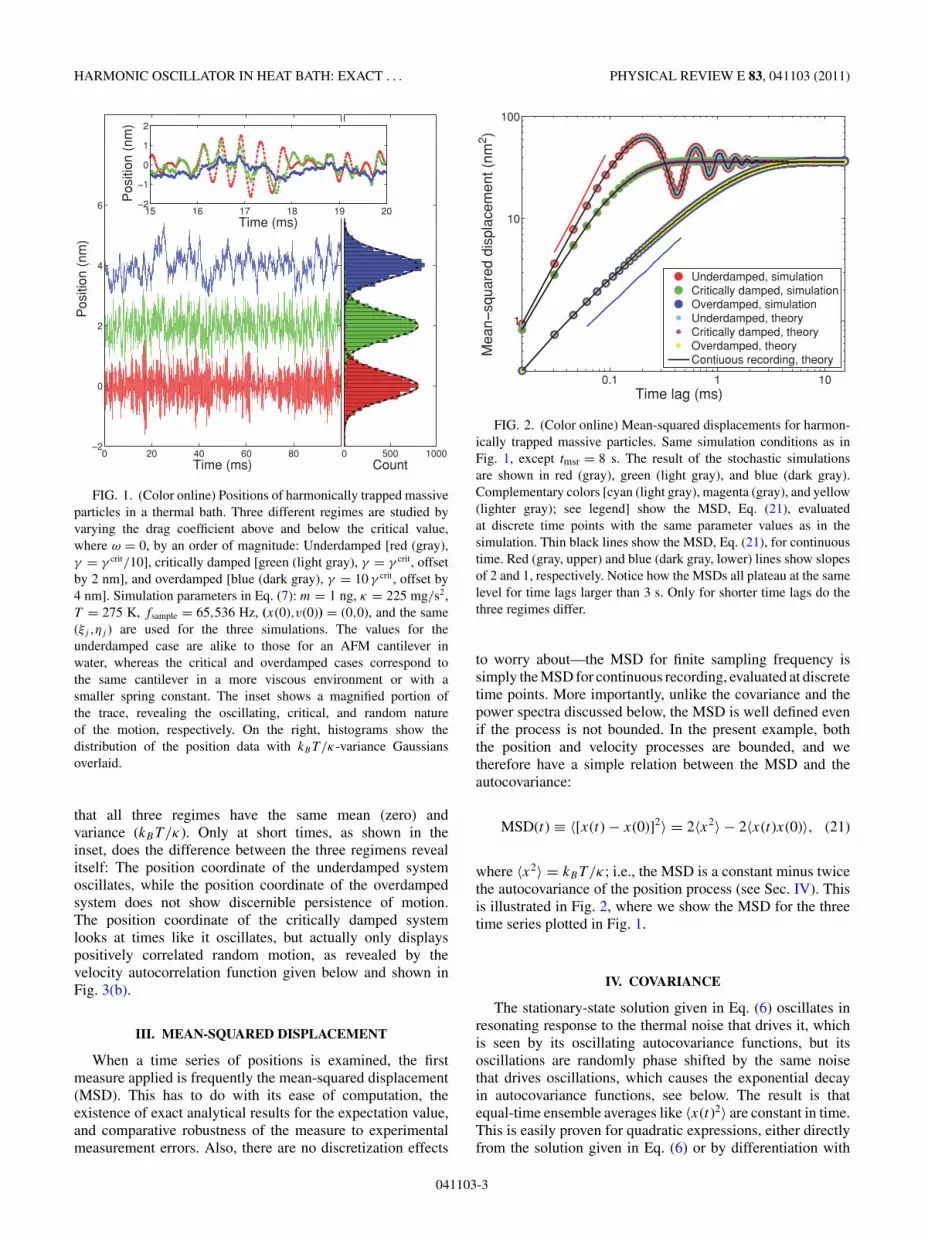
FIG. 1. (Color online) Positions of harmonically trapped massiveparticles in a thermal bath. Three different regimes are studied byvarying the drag coefficient above and below the critical value,where ω = 0, by an order of magnitude: Underdamped [red (gray),γ = γ crit/10], critically damped [green (light gray), γ = γ crit, offsetby 2 nm], and overdamped [blue (dark gray), γ = 10 γ crit, offset by4 nm]. Simulation parameters in Eq. (7): m = 1 ng, κ = 225 mg/s2,T = 275 K, fsample = 65,536 Hz, (x(0),v(0)) = (0,0), and the same(ξj ,ηj ) are used for the three simulations. The values for theunderdamped case are alike to those for an AFM cantilever inwater, whereas the critical and overdamped cases correspond tothe same cantilever in a more viscous environment or with asmaller spring constant. The inset shows a magnified portion ofthe trace, revealing the oscillating, critical, and random natureof the motion, respectively. On the right, histograms show thedistribution of the position data with kBT /κ-variance Gaussiansoverlaid.

that all three regimes have the same mean (zero) andvariance (kBT /κ). Only at short times, as shown in theinset, does the difference between the three regimens revealitself: The position coordinate of the underdamped systemoscillates, while the position coordinate of the overdampedsystem does not show discernible persistence of motion.The position coordinate of the critically damped systemlooks at times like it oscillates, but actually only displayspositively correlated random motion, as revealed by thevelocity autocorrelation function given below and shown inFig. 3(b).

III. MEAN-SQUARED DISPLACEMENT

When a time series of positions is examined, the firstmeasure applied is frequently the mean-squared displacement(MSD). This has to do with its ease of computation, theexistence of exact analytical results for the expectation value,and comparative robustness of the measure to experimentalmeasurement errors. Also, there are no discretization effects

0.1 1 10

1

10

100

Time lag (ms)

Mea

nsq

uare

d di

spla

cem

ent (

nm2 )

Underdamped, simulationCritically damped, simulationOverdamped, simulationUnderdamped, theoryCritically damped, theoryOverdamped, theoryContiuous recording, theory

FIG. 2. (Color online) Mean-squared displacements for harmon-ically trapped massive particles. Same simulation conditions as inFig. 1, except tmsr = 8 s. The result of the stochastic simulationsare shown in red (gray), green (light gray), and blue (dark gray).Complementary colors [cyan (light gray), magenta (gray), and yellow(lighter gray); see legend] show the MSD, Eq. (21), evaluatedat discrete time points with the same parameter values as in thesimulation. Thin black lines show the MSD, Eq. (21), for continuoustime. Red (gray, upper) and blue (dark gray, lower) lines show slopesof 2 and 1, respectively. Notice how the MSDs all plateau at the samelevel for time lags larger than 3 s. Only for shorter time lags do thethree regimes differ.

to worry about—the MSD for finite sampling frequency issimply the MSD for continuous recording, evaluated at discretetime points. More importantly, unlike the covariance and thepower spectra discussed below, the MSD is well defined evenif the process is not bounded. In the present example, boththe position and velocity processes are bounded, and wetherefore have a simple relation between the MSD and theautocovariance:

MSD(t) ≡ ⟨[x(t) − x(0)]2⟩ = 2⟨x2⟩ − 2⟨x(t)x(0)⟩, (21)

where ⟨x2⟩ = kBT /κ; i.e., the MSD is a constant minus twicethe autocovariance of the position process (see Sec. IV). Thisis illustrated in Fig. 2, where we show the MSD for the threetime series plotted in Fig. 1.

IV. COVARIANCE

The stationary-state solution given in Eq. (6) oscillates inresonating response to the thermal noise that drives it, whichis seen by its oscillating autocovariance functions, but itsoscillations are randomly phase shifted by the same noisethat drives oscillations, which causes the exponential decayin autocovariance functions, see below. The result is thatequal-time ensemble averages like ⟨x(t)2⟩ are constant in time.This is easily proven for quadratic expressions, either directlyfrom the solution given in Eq. (6) or by differentiation with

041103-3


respect to time using Ito’s lemma:

d

dt

⎛

⎜⎝⟨x2⟩⟨xv⟩⟨v2⟩

⎞

⎟⎠

=

⎛

⎜⎝0 2 0

−ω20

−1τ

1

0 −2ω20

−2τ

⎞

⎟⎠

⎛

⎜⎝⟨x2⟩⟨xv⟩⟨v2⟩

⎞

⎟⎠ +

⎛

⎝00

2Dτ 2

⎞

⎠ . (22)

As is seen by inspection, this equation has the time-independent solution

⎛

⎜⎜⎝

⟨x2⟩⟨xv⟩

⟨v2⟩

⎞

⎟⎟⎠ =

⎛

⎜⎜⎝

kBTκ

0kBTm

⎞

⎟⎟⎠ , (23)

in accord with the equipartition theorem. This solution is theunique attractor for the system’s dynamics: Left to itself, anydiscrepancy from this time-independent solution will decreaseto zero exponentially fast in time—possibly while oscillatingharmonically with cyclic frequency 2ω—as is seen from thefact that the 3 × 3 matrix in Eq. (23) has eigenvalues −1/τand −1/τ ± i2ω, and determinant −4ω2

0/τ .Similar reasoning [or simply multiplying Eq. (7) by

(xj ,vj ), then taking the expectation value and applying theequipartition theorem] gives the covariances

( ⟨x(t)x(0)⟩ ⟨x(t)v(0)⟩⟨v(t)x(0)⟩ ⟨v(t)v(0)⟩

).

= D

τe− t

2τ

( cos ωt+ sin ωt2ωτ

ω20

sin ωtω

− sin ωtω

cos ωt − sin ωt2ωτ

)

. (24)

For ω real (underdamped system), these covariances oscillate,we see, with amplitudes that decrease exponentially in timewith characteristic time 2τ . For ω imaginary (overdampedsystem), we rewrite Eq. (24) as

(⟨x(t)x(0)⟩ ⟨x(t)v(0)⟩⟨v(t)x(0)⟩ ⟨v(t)v(0)⟩

)

= D

2|ω|τ

{( 1ω2

0τ+1

−1 −1τ−

)

e−t/τ− +( −1

ω20τ−

−1

1 1τ+

)

e−t/τ+

}

,

(25)

from which we see that the system decreases as a doubleexponential with characteristic times τ± = 2τ/(1 ± 2τ |ω|). Atcritical damping (ω = 0), the expressions for the covariancessimplify to

( ⟨x(t)x(0)⟩ ⟨x(t)v(0)⟩⟨v(t)x(0)⟩ ⟨v(t)v(0)⟩

)

= D

τe− t

2τ

( 1+t/(2τ )ω2

0t

−t 1 − t/(2τ )

)

. (26)

Figure 3 illustrates these dynamics for the normalized covari-ances, a.k.a. the correlation functions.

As is the case for the MSD, there are no discretizationeffects to worry about—the covariance for finite samplingfrequency is simply the covariance for continuous recording,

0.1 1 101

0.5

0

0.5

1

Time lag (ms)

Vel

ocity

aut

ocor

rela

tion

exp[ t/(2 )]

(b)

0.1 1 101

0.5

0

0.5

1

Time lag (ms)

Pos

ition

aut

ocor

rela

tion

exp[ t/(2 )]

0.1 1 101

0.5

0

0.5

1

Time lag (ms)

Pos

ition

velo

city

cro

ssco

rrel

atio

n

exp[ t/(2 )]

(a)

(c)

FIG. 3. (Color online) Correlation functions, Eq. (24), for mas-sive particles in a harmonic potential, driven by thermal noise.Color coding and simulation settings are the same as in Fig. 2: Red(gray), green (light gray), and blue (dark gray) show the result of astochastic simulation; complementary colors show the covariance(not a fit), Eq. (24), normalized and evaluated at discrete timepoints; thin black lines show the covariance for continuous time(not a fit); and dashed red (gray) lines show the enveloping expo-nential exp(−t/(2τ )). (a) Position autocorrelations, ⟨x(t)x(0)⟩/⟨x2⟩.(b) Velocity autocorrelations, ⟨v(t)v(0)⟩/⟨v2⟩. (c) Position-velocitycross correlations, ⟨x(t)v(0)⟩/

√⟨x2⟩⟨v2⟩. The velocity-position cross

correlation, ⟨v(t)x(0)⟩/√

⟨x2⟩⟨v2⟩ (not shown), has the opposite signbut is otherwise identical.

041103-4


0 0.05 0.1

0

0.5

1

Time lag (ms)

0.1 1 101

0.5

0

0.5

1

Time lag (ms)

Vel

ocity

aut

ocor

rela

tion

Underdamped, secant theoryCritically damped, secant theoryOverdamped, secant theory

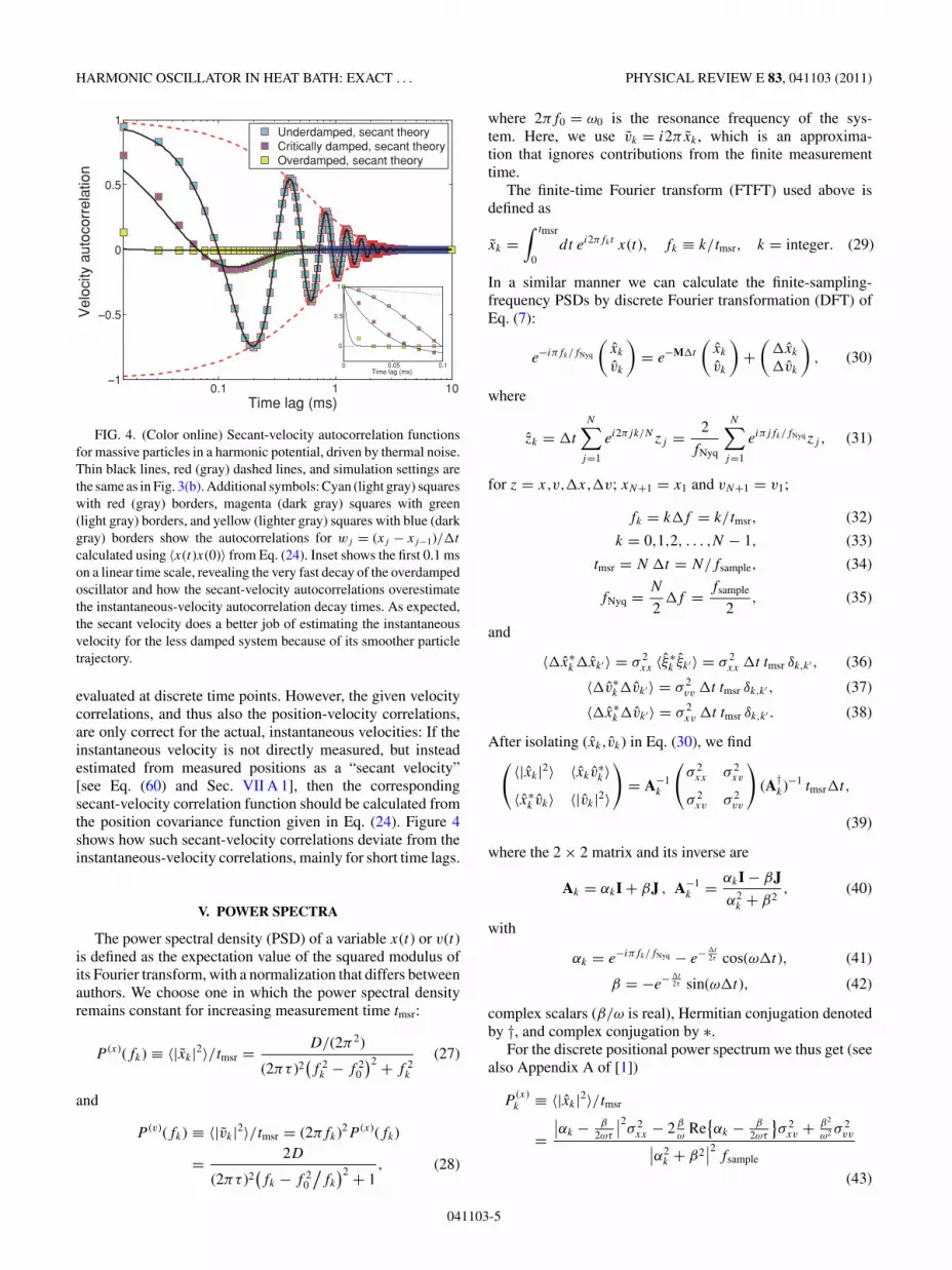
FIG. 4. (Color online) Secant-velocity autocorrelation functionsfor massive particles in a harmonic potential, driven by thermal noise.Thin black lines, red (gray) dashed lines, and simulation settings arethe same as in Fig. 3(b). Additional symbols: Cyan (light gray) squareswith red (gray) borders, magenta (dark gray) squares with green(light gray) borders, and yellow (lighter gray) squares with blue (darkgray) borders show the autocorrelations for wj = (xj − xj−1)/'t

calculated using ⟨x(t)x(0)⟩ from Eq. (24). Inset shows the first 0.1 mson a linear time scale, revealing the very fast decay of the overdampedoscillator and how the secant-velocity autocorrelations overestimatethe instantaneous-velocity autocorrelation decay times. As expected,the secant velocity does a better job of estimating the instantaneousvelocity for the less damped system because of its smoother particletrajectory.

evaluated at discrete time points. However, the given velocitycorrelations, and thus also the position-velocity correlations,are only correct for the actual, instantaneous velocities: If theinstantaneous velocity is not directly measured, but insteadestimated from measured positions as a “secant velocity”[see Eq. (60) and Sec. VII A 1], then the correspondingsecant-velocity correlation function should be calculated fromthe position covariance function given in Eq. (24). Figure 4shows how such secant-velocity correlations deviate from theinstantaneous-velocity correlations, mainly for short time lags.

V. POWER SPECTRA

The power spectral density (PSD) of a variable x(t) or v(t)is defined as the expectation value of the squared modulus ofits Fourier transform, with a normalization that differs betweenauthors. We choose one in which the power spectral densityremains constant for increasing measurement time tmsr:

P (x)(fk) ≡ ⟨|xk|2⟩/tmsr = D/(2π2)

(2πτ )2(f 2

k − f 20

)2 + f 2k

(27)

and

P (v)(fk) ≡ ⟨|vk|2⟩/tmsr = (2πfk)2P (x)(fk)

= 2D

(2πτ )2(fk − f 2

0

/fk

)2 + 1, (28)

where 2πf0 = ω0 is the resonance frequency of the sys-tem. Here, we use vk = i2π xk , which is an approxima-tion that ignores contributions from the finite measurementtime.

The finite-time Fourier transform (FTFT) used above isdefined as

xk =∫ tmsr

0dt ei2πfkt x(t), fk ≡ k/tmsr, k = integer. (29)

In a similar manner we can calculate the finite-sampling-frequency PSDs by discrete Fourier transformation (DFT) ofEq. (7):

e−iπfk/fNyq

(xk

vk

)= e−M't

(xk

vk

)+

('xk

'vk

), (30)

where

zk = 't

N∑

j=1

ei2πjk/Nzj = 2fNyq

N∑

j=1

eiπjfk/fNyqzj , (31)

for z = x,v,'x,'v; xN+1 = x1 and vN+1 = v1;

fk = k'f = k/tmsr, (32)

k = 0,1,2, . . . ,N − 1, (33)

tmsr = N 't = N/fsample, (34)

fNyq = N

2'f =

fsample

2, (35)

and

⟨'x∗k 'xk′ ⟩ = σ 2

xx ⟨ξ ∗k ξk′ ⟩ = σ 2

xx 't tmsr δk,k′ , (36)

⟨'v∗k'vk′ ⟩ = σ 2

vv 't tmsr δk,k′ , (37)

⟨'x∗k 'vk′ ⟩ = σ 2

xv 't tmsr δk,k′ . (38)

After isolating (xk,vk) in Eq. (30), we find(

⟨|xk|2⟩ ⟨xkv∗k ⟩

⟨x∗k vk⟩ ⟨|vk|2⟩

)

= A−1k

(σ 2

xx σ 2xv

σ 2xv σ 2

vv

)

(A†k)−1 tmsr't,

(39)

where the 2 × 2 matrix and its inverse are

Ak = αkI + βJ , A−1k = αkI − βJ

α2k + β2

, (40)

with

αk = e−iπfk/fNyq − e− 't2τ cos(ω't), (41)

β = −e− 't2τ sin(ω't), (42)

complex scalars (β/ω is real), Hermitian conjugation denotedby †, and complex conjugation by ∗.

For the discrete positional power spectrum we thus get (seealso Appendix A of [1])

P(x)k ≡ ⟨|xk|2⟩/tmsr

=∣∣αk − β

2ωτ

∣∣2σ 2

xx − 2 βω

Re{αk − β

2ωτ

}σ 2

xv + β2

ω2 σ2vv∣∣α2

k + β2∣∣2

fsample

(43)

041103-5


whereas the discrete velocity power spectrum is

P(v)k ≡ ⟨|vk|2⟩/tmsr

=∣∣αk + β

2ωτ

∣∣2σ 2

vv + 2ω20

βω

Re{αk + β

2ωτ

}σ 2

xv + ω40

β2

ω2 σ2xx∣∣α2

k + β2∣∣2

fsample

.

(44)

In the case of critical damping (ω = 0) we simply insert β/ω =−e− 't

2τ 't in Eqs. (43) and (44), and use Eqs. (18), (19), and(20) for the variance-covariances.

Figure 5 shows the power spectra that result from numericalsimulations of AFM cantilever positions and velocities usingEq. (7) for three different drag coefficients, as well as thecorresponding analytical expressions as given in Eqs. (43)and (44).

An alternative route to these discrete PSDs is to take thediscrete Fourier transform of the covariance function from theprevious section: Both the position and the velocity processesare stationary (the joint probability density function for each isindependent of time), so the Wiener-Khinchin theorem appliesand the Fourier transform of the correlation function is equal tothe PSD. For vanishing spring constant κ , the position processis unbounded (not stationary) and the covariance, as well asthe PSD, is consequently ill defined. This limit is treated inSec. VII A.

Note, the PSD for discretely measured (instantaneous)velocities, Eq. (44), should not be confused with the discretePSD for secant velocities, Eq. (61). The latter is the correctexpression to use in experiments where the velocities areestimated from the measured positions.

VI. VANISHING !t: THE LIMIT OF CONTINUOUSRECORDING

As 't → 0 we find to first order in 't that the covariancesin Eqs. (15)–(20) reduce to σ 2

xx = 0, σ 2vv = 2D't/τ 2, and

σ 2xv = 0. That is, 'xj = 0 and 'vj = σvvζj =

√2D't/τ ζj .

In other words, the velocity process is seen to be driving theposition process.

In this limit the positional PSD takes on the familiar formgiven in Eq. (27), and the velocity PSD is given in Eq. (28).Comparing the continuous-recording PSDs, Eqs. (27) and(28), with their discrete sampling analogues, Eqs. (43) and(44), we see in Fig. 5(a) that they differ substantially at highfrequencies, and in Fig. 5(b) that they differ everywhere butnear f0 in the underdamped case. Thus, one should not attemptto fit a theoretical PSD derived for “continuously recorded”trajectories to an experimental PSD, which necessarily isobtained with time-lapse recording. More specifically, oneshould only attempt to fit it to the low-frequency part of theexperimental spectrum for positions, or account for “aliasing”before fitting, as described, e.g., in Appendix H of [9], whichturns Eqs. (27) and (28) into Eqs. (43) and (44), respectively.

The position covariance and the MSD do not suffer from thisdichotomy. Neither of them changes its shape or form whenswitching between discrete and continuous time: The discreteversions are equal to the continuous versions, evaluated atdiscrete times:

⟨xjxj+ℓ⟩ = ⟨x(tj )x(tj+ℓ)⟩ = ⟨x(0)x(tℓ)⟩ (45)

101

102

103

104

1018

1017

1016

1015

1014

1013

1012

Frequency (Hz)

PS

D/

(m2 s2 /k

g)

Underdamped, simulationCritically damped, simulationOverdamped, simulationUnderdamped, theoryCritically damped, theoryOverdamped, theoryContinuous recording, theory

101

102

103

104

108

107

106

105

104

103

Frequency (Hz)

PS

D/

(m2 /k

g)

Underdamped, simulationCritically damped, simulationOverdamped, simulationUnderdamped, theoryCritically damped, theoryOverdamped, theoryContinuous recording, theoryAliased theory

(a)

(b)

FIG. 5. (Color online) Power spectra for positions and velocitiesof harmonically trapped massive particles in thermal bath, normalizedby γ . The color scheme is the same as in Figs. 2 and 3: Synthetic dataare shown in red (gray), green (light gray), and blue (dark gray); thealiased theory, Eqs. (43) and (44), is shown in complementary colors;and the nonaliased theory, Eqs. (27) and (28), as thin black lines.Simulation parameters are as in Fig. 1 (giving ω0 = 15 kHz) withnwin = 32 Hann windows applied to the tmsr = 8 s long time series. (a)Power spectra for positions. Thin blue (dark gray, lower) and red (gray,upper) lines illustrate f −2 and f −4 behaviors, respectively. Notice thedisagreement between the nonaliased (continuous recording) theoryand data at high frequencies. (b) Power spectra for velocities. Dashedblack lines show aliased versions of Eq. (28); i.e., P (v,aliased)(f ) =∑∞

n=−∞ P (v)(f + nfsample) [9], here truncated to 201 terms. Thenonaliased theory severely underestimates the power at high and lowfrequencies, and completely misses the data in the overdamped case.

and

⟨(xj − xj+ℓ)2⟩ = ⟨[x(tj ) − x(tj+ℓ)]2⟩ = ⟨[x(0) − x(tℓ)]2⟩,(46)

where, in the last step, we used that the process is stationary andthe measures therefore invariant to time translations. That is,these measures are unaffected by the unavoidable discretenessof real-world data.

041103-6


The velocity’s covariance is also unaffected by time-lapserecording, if we can measure the instantaneous velocity, i.e.,the velocity vector that is tangential to the trajectory of theposition. If we cannot and time-lapse-record only positions,we have a different situation, which is treated below.

VII. VARIOUS PHYSICAL LIMITS: A REFERENCE SETOF FORMULAS

Three physical limiting cases are of particular interest:(i) Vanishing spring constant, κ = 0, which is the Ornstein-Uhlenbeck theory for Brownian motion for a free particlewith inertia; (ii) vanishing mass, m = 0, which is Einstein’stheory for Brownian motion of a particle trapped by a Hookeanforce, and a popular minimalist model of the Brownian motionof a microsphere in an optical trap; and (iii) vanishing massand spring constant, which is Einstein’s theory for Brownianmotion of a free particle.

A. Vanishing spring constant: The Ornstein-Uhlenbeck process

When there is no Hookean restoring force κ = 0, Eq. (1)describes the free diffusion of a massive particle according toOrnstein and Uhlenbeck [4]:

mv(t) + γ v(t) = Ftherm(t). (47)

This velocity process is known as the Ornstein-Uhlenbeck(OU) process [4]. When modeling other dynamical systems,such as migrating cells, m does not refer to the physical mass ofthe cell but rather its inertia to velocity changes, or persistenceof motion; likewise γ is not the friction between the cell andsubstrate but describes the rate of memory loss for the velocityprocess. The structure of Eqs. (7), (9), (10), (13), and (14)remains the same; the only change is ω0 = 0 in Eq. (10),hence ω = i/(2τ ), and the covariances, Eqs. (15), (16), and(17), consequently reduce to

σ 2xx = Dτ [2't/τ − 4(1 − a) + (1 − a2)], (48)

σ 2vv = D(1 − a2)/τ, (49)

σ 2xv = D (1 − a)2 , (50)

where

a = e−'t/τ , τ = m/γ . (51)

For the velocity and position processes we thus find

vj+1 = avj + 'vj , (52)

xj+1 = xj + τ (1 − a)vj + 'xj . (53)

That is, the velocity process has reduced to a stable autoregres-sive model of order 1, AR(1). Its time integral, the positionprocess, is unbounded—the particle is diffusing freely andwithout limits. Exact numerical update formulas for vj and xj

have previously been given in [3]; here we rederived them forconsistency of notation.

The discrete-time positional PSD, P(x)k , is obtainable from

Eq. (43) with ω0 = 0 and the σ s given in Eqs. (48), (49), and(50); the expression does not simplify significantly comparedto Eq. (43). The discrete-time velocity PSD, P

(v)k , is much

simpler and can be derived directly from the discrete-timevelocity process, Eq. (52), or by taking the κ = 0 limit of

Eq. (44). From these discrete-time PSDs the continuous-recording expressions, P (x)(fk) and P (v)(fk), can be obtainedby expanding to leading order in 't/τ and k/N = fk/fsample;or they can be derived directly from the continuous-timeequation of motion Eq. (47) by Fourier transformation and, forthe positional PSD, remembering that x = v. The continuous-recording positional PSD and the two velocity PSDs then read

P (x)(fk) = D/(2π2)(2πτ )2f 4

k + f 2k

, (54)

P(v)k = σ 2

vv 't

1 + a2 − 2a cos(2πk/N), (55)

P (v)(fk) = 2D

1 + (2πfkτ )2. (56)

Note that the positional PSD diverges in fk = 0 due to theprocess being unbounded. This implies that we cannot use theWiener-Khinchin theorem to obtain the covariance by Fouriertransforming the PSDs, and vice versa. The velocity process isbounded, however, and the velocity correlation functions arestraightforward to calculate, so we simply list the results forthe discrete and the continuous cases:

⟨vivj ⟩ = D

τe−|i−j |'t/τ , (57)

⟨v(t)v(t ′)⟩ = D

τe−|t−t ′|/τ . (58)

As already mentioned, the time integral of the OU processis one of the instances where the mean-squared displacementprovides a useful measure for the position process, while thepositional covariance function is ill defined. The mean-squareddisplacement of the time integral of the OU process is

⟨[x(t) − x(0)]2⟩ = 2Dτ (t/τ + e−t/τ − 1). (59)

For t ≪ τ this MSD increases as t2 (ballistically) and fort ≫ τ as t (diffusively), with an exponential crossover betweenthe two regimes with characteristic time τ .

1. Secant velocities

In experiments, the velocity is typically not measureddirectly, but approximated from the measured positions as a“secant velocity”:

wj = (xj − xj−1)/'t (60)

with discrete power spectral density

P(w)k ≡ ⟨|wk|2⟩/tmsr =

2[1 − cos(πfk/fNyq)]('t)2

P(x)k . (61)

This is a general result that follows from the definition of wj

and is independent of the dynamic model.For the OU process, we can relate this PSD to the PSD for

the continuous velocity that it approximates, if we rewrite it as

P(w)k = P

(v)k (τ/'t)2(1 − a)2 + σ 2

xx/'t

+ τ (1 − a)(⟨v∗k 'xk⟩ + c.c.). (62)

Here the first term is proportional to P(v)k , the second term

is a constant, and the last term is frequency dependent withc.c., the complex conjugate of the other term in the bracket.However, it is not easy to see from this expression how much

041103-7


P(w)k deviates from P

(v)k . We can get a good idea about the

shape of the PSD from the autocorrelation function,

⟨w2j ⟩ = 2⟨v2

j ⟩(

τ

't

)2

('t/τ − 1 + a) (63)

≈ ⟨v2j ⟩

(1 − 1

3't/τ

), (64)

and for ℓ > 0,

⟨wjwj+ℓ⟩ = 2⟨vjvj+ℓ⟩(

τ

't

)2

[cosh('t/τ ) − 1] (65)

≈ ⟨vjvj+ℓ⟩(

1 + 112

('t/τ )2)

, (66)

where we used Eqs. (13), (14), (50), (53), and (57) to deriveEqs. (63) and (65)—the latter two expressions are proportionalto the velocity autocorrelations they approximate; they onlydiffer by multiplicative factors that are independent of thetime lag for ℓ > 0. To first order in 't/τ we thus have, forℓ ! 0,

⟨wjwj+ℓ⟩ = ⟨vjvj+ℓ⟩(

1 − 13

't

τδ0,ℓ

). (67)

We now apply the Wiener-Khinchin theorem to get the PSDas the Fourier transform of this approximated auto-correlationfunction and find

P(w)k ≈ P

(v)k − 1

3

('t

τ

)2

D. (68)

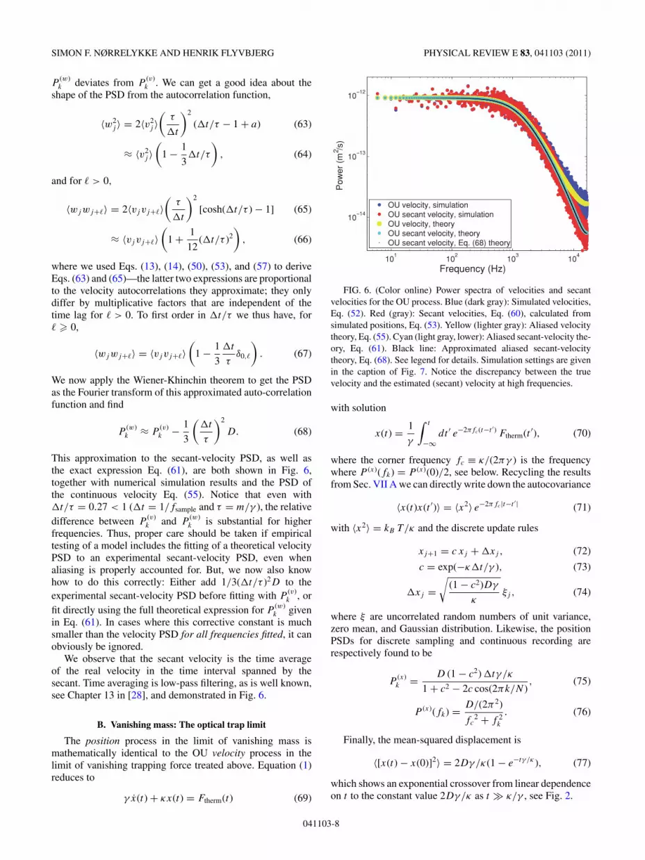
This approximation to the secant-velocity PSD, as well asthe exact expression Eq. (61), are both shown in Fig. 6,together with numerical simulation results and the PSD ofthe continuous velocity Eq. (55). Notice that even with't/τ = 0.27 < 1 ('t = 1/fsample and τ = m/γ ), the relativedifference between P

(v)k and P

(w)k is substantial for higher

frequencies. Thus, proper care should be taken if empiricaltesting of a model includes the fitting of a theoretical velocityPSD to an experimental secant-velocity PSD, even whenaliasing is properly accounted for. But, we now also knowhow to do this correctly: Either add 1/3('t/τ )2D to theexperimental secant-velocity PSD before fitting with P

(v)k , or

fit directly using the full theoretical expression for P(w)k given

in Eq. (61). In cases where this corrective constant is muchsmaller than the velocity PSD for all frequencies fitted, it canobviously be ignored.

We observe that the secant velocity is the time averageof the real velocity in the time interval spanned by thesecant. Time averaging is low-pass filtering, as is well known,see Chapter 13 in [28], and demonstrated in Fig. 6.

B. Vanishing mass: The optical trap limit

The position process in the limit of vanishing mass ismathematically identical to the OU velocity process in thelimit of vanishing trapping force treated above. Equation (1)reduces to

γ x(t) + κx(t) = Ftherm(t) (69)

101

102

103

104

1014

1013

1012

Frequency (Hz)

Pow

er (m

2 /s)

OU velocity, simulationOU secant velocity, simulationOU velocity, theoryOU secant velocity, theoryOU secant velocity, Eq. (68) theory

FIG. 6. (Color online) Power spectra of velocities and secantvelocities for the OU process. Blue (dark gray): Simulated velocities,Eq. (52). Red (gray): Secant velocities, Eq. (60), calculated fromsimulated positions, Eq. (53). Yellow (lighter gray): Aliased velocitytheory, Eq. (55). Cyan (light gray, lower): Aliased secant-velocity the-ory, Eq. (61). Black line: Approximated aliased secant-velocitytheory, Eq. (68). See legend for details. Simulation settings are givenin the caption of Fig. 7. Notice the discrepancy between the truevelocity and the estimated (secant) velocity at high frequencies.

with solution

x(t) = 1γ

∫ t

−∞dt ′ e−2πfc(t−t ′) Ftherm(t ′), (70)

where the corner frequency fc ≡ κ/(2πγ ) is the frequencywhere P (x)(fk) = P (x)(0)/2, see below. Recycling the resultsfrom Sec. VII A we can directly write down the autocovariance

⟨x(t)x(t ′)⟩ = ⟨x2⟩ e−2πfc |t−t ′| (71)

with ⟨x2⟩ = kB T /κ and the discrete update rules

xj+1 = c xj + 'xj , (72)

c = exp(−κ't/γ ), (73)

'xj =√

(1 − c2)Dγ

κξj , (74)

where ξ are uncorrelated random numbers of unit variance,zero mean, and Gaussian distribution. Likewise, the positionPSDs for discrete sampling and continuous recording arerespectively found to be

P(x)k = D (1 − c2) 'tγ /κ

1 + c2 − 2c cos(2πk/N), (75)

P (x)(fk) = D/(2π2)

fc2 + f 2

k

. (76)

Finally, the mean-squared displacement is

⟨[x(t) − x(0)]2⟩ = 2Dγ /κ(1 − e−tγ /κ ), (77)

which shows an exponential crossover from linear dependenceon t to the constant value 2Dγ /κ as t ≫ κ/γ , see Fig. 2.

041103-8


C. Vanishing mass and spring constant: Einstein’sBrownian motion

When both m = 0 and κ = 0, Eq. (1) reduces to

γ x(t) = Ftherm(t) (78)

so that

xj+1 = xj +√

2D 't ξj , (79)

where

ξj ≡ 1√'t

∫ tj+1

tj

dt η(t), (80)

hence

⟨ξj ⟩ = 0, ⟨ξiξj ⟩ = δi,j , (81)

and the velocity and position PSDs for discrete and continuoussampling take on the simple forms:

P(x)k =

D/fsample2

2 sin2(πfk/fsample), (82)

P (x)(fk) = D

2π2f 2k

, (83)

P(v)k = P (v)(fk) = 2D. (84)

101

102

103

104

1020

1015

Frequency (Hz)

Pow

er (m

2 s)

EB, simulationOT, simulationOU, simulationEB, theoryOT, theoryOU, theoryContinuous recording, theory

FIG. 7. (Color online) Power spectra of positions. Green points(light gray): Freely diffusing massless particle (Einstein’s Brownianmotion); red points (gray): trapped massless particle (OT limit, orOU velocity process); and blue (dark gray) points: freely diffusingmassive particles (time integral of OU process). Complementarycolors show the finite sampling frequency (aliased) theories, whereasthe continuous recording (nonaliased) theories are shown as thinblack lines. Green (light gray, upper) and blue (dark gray, lower) linesindicate f −2 and f −4 behavior, respectively. See legend for details.Simulation parameters: D = 0.46 µm2/s, T = 275 K, m = 1 ng,fc = 500 Hz, fsample = 32 768 Hz, N = 131 072, and nwin = 32 Hannwindows. The simulation parameters for the OT case are those of a1 µm diameter polystyrene sphere held in an optical trap in water atroom temperature. The parameters for Einstein’s Brownian motionare the same, except κ = 0. For the OU process we increased thedensity of the sphere roughly 2000 times, which is not a physicallyrealistic scenario but allows us to plot all power spectra with the sameaxes.

0.1 1 101

100

1000

Time lag (ms)

Mea

nsq

uare

d di

spla

cem

ent (

nm2 )

EB, simulationOT, simulationOU, simulationEB, theoryOT, theoryOU, theoryContinuous recording, theory

FIG. 8. (Color online) Mean-squared displacement for theOrnstein-Uhlenbeck, optical-trap, and Brownian-motion limits de-scribed in Secs. VII A, VII B and VII C. Simulation settings andlegends are the same as in Fig. 7, except green (light gray, upper) andblue (dark gray, lower) lines show slopes of 1 and 2, respectively.

As was the case for the time integral of the OU pro-cess, the position PSDs are singular in fk = 0 because theprocess is unbounded. That is, the meaningful measure tostudy is not the covariance, but rather the mean-squareddisplacement

⟨[x(t) − x(0)]2⟩ = 2Dt, (85)

which is one of the few well-defined statistics for Einstein’stheory of Brownian motion: Because the trajectory of positionsis a fractal, attempts at estimating the average speed ofBrownian motion from the displacement of position occurringin a given time interval will depend on the duration, 't , of thisinterval as 1/

√'t , hence diverge when accuracy is sought

improved by reducing 't . This was not appreciated beforeEinstein’s 1905 paper on the subject.

Figures 7 and 8 show the power spectra and mean-squareddisplacements, respectively, obtained in numerical simulationsof free diffusion and trapped diffusion, as well as the graphs ofthe corresponding analytical expressions. At short time scales,i.e., at high frequencies in Fig. 7 and for small time lags inFig. 8, the thermal forces dominate and the Hookean forcehas not had time to influence the motion through its constant,but weak, confining effect. That is why the Brownian motion(green) and optical trap (red) data collapse in this regime,whereas the Ornstein-Uhlenbeck process (blue) differs fromthe two due to inertial effects. Conversely, at long time scales,low frequencies in Fig. 7, and large time lags in Fig. 8,inertia plays no role, so the Ornstein-Uhlenbeck process andEinstein’s theory of Brownian motion are indistinguishable,whereas the Hookean force has had time to exert its confiningeffect on the optical trap data.

VIII. SUMMARY AND CONCLUSIONS

We examined the dampened harmonic oscillator and threeof its physical limits: The massless case (optical trap), the freecase (the Einstein-Ornstein-Uhlenbeck theory of Brownian

041103-9


motion), and the massless free case (Einstein’s Brownianmotion). By solving the system’s dynamical equations foran arbitrary time lapse 't , exact analytical expressions werederived for the changes in position and velocity duringsuch a time lapse. With these expressions, exact simula-tions of the dynamics are then possible—with an accuracythat is independent of the duration of the time lapse. Incontrast, a numerical simulation, using Euler integrationor similar schemes, is exact only to first or second orderin 't [29].

We gave exact analytical expressions for power-spectralforms, mean-squared displacements, and correlation functionsthat can be fitted (see [1] before undertaking a least-squares fit)to data obtained from time-lapse recording of a system withdynamics similar to the dampened harmonic oscillator or one

of its three physical limits described here. The effect of finitesampling rates (aliasing) were also discussed.

The effect on the power spectrum of velocity estimationfrom position data (secant velocity) was treated for the caseof free diffusion of a massive particle. Approximate as well asexact corrective factors and expressions were given. Through-out, we pointed out when power spectral analysis makessense (bounded process) or does not, which of the statisticalmeasures depend on the sampling frequency, and which maybe described by the simpler continuous-time theory.

ACKNOWLEDGMENTS

S.F.N. gratefully acknowledges financial support from theCarlsberg Foundation and the Lundbeck Foundation.

[1] S. F. Nørrelykke and H. Flyvbjerg, Rev. Sci. Instrum. 81, 075103(2010).

[2] L. Schimansky-Geier and C. Zulicke, Z. Phys. B 79, 451 (1990).[3] D. T. Gillespie, Phys. Rev. E 54, 2084 (1996).[4] G. Uhlenbeck and L. Ornstein, Phys. Rev. 36, 823 (1930).[5] S. Chandrasekhar, Rev. Mod. Phys. 15, 0001 (1943).[6] M. C. Wang and G. E. Uhlenbeck, Rev. Mod. Phys. 17, 323

(1945).[7] L. S. Ornstein, Proc. R. Acad. Amsterdam 21, 96 (1919).[8] H. A. Lorentz, Lessen over Theoretishe Natuurkunde, Vol. V

(E. J. Brill, Leiden, 1921), Chap. Kinetische Problemen.[9] K. Berg-Sørensen and H. Flyvbjerg, Rev. Sci. Instrum. 75, 594

(2004).[10] K. Berg-Sørensen, E. J. G. Peterman, T. Weber, C. F. Schmidt,

and H. Flyvbjerg, Rev. Sci. Instrum. 77, 063106 (2006).[11] B. Lukic, S. Jeney, C. Tischer, A. J. Kulik, L. Forro, and E.-L.

Florin, Phys. Rev. Lett. 95, 160601 (2005).[12] D. Selmeczi, S. F. Tolic-Nørrelykke, E. Schaffer, P. H. Hagedorn,

S. Mosler, K. Berg-Sørensen, N. B. Larsen, and H. Flyvbjerg,Acta Phys. Pol. B 38, 2407 (2007).

[13] D. R. Burnham and D. McGloin, New J. Phys. 11, 063022(2009).

[14] D. R. Burnham, P. J. Reece, and D. McGloin, Phys. Rev. E 82,051123 (2010).

[15] T. Li, S. Kheifets, D. Medellin, and M. G. Raizen, Science 328,1673 (2010).

[16] J. Sader, J. Appl. Phys. 84, 64 (1998).[17] M. H. Gail and C. W. Boone, Biophys. J. 10, 980 (1970).[18] R. L. Hall, J. Math. Biol. 4, 327 (1977).[19] U. Euteneuer and M. Schliwa, Nature (London) 310, 58

(1984).[20] D. Selmeczi, S. Mosler, P. H. Hagedorn, N. B. Larsen, and

H. Flyvbjerg, Biophys. J. 89, 912 (2005).[21] D. Selmeczi, L. Li, L. I. I. Pedersen, S. F. Nørrelykke, P. H.

Hagedorn, S. Mosler, N. B. Larsen, E. C. Cox, and H. Flyvbjerg,Eur. Phys. J. Spec. Top. 157, 1 (2008).

[22] L. Li, E. C. Cox, and H. Flyvbjerg (submitted 2011).[23] L. Li, S. F. Nørrelykke, and E. C. Cox, PLoS ONE 3, e2093

(2008).[24] E. A. Codling, M. J. Plank, and S. Benhamou, J. R. Soc. Interface

5, 813 (2008).[25] E. Schwartz and J. Smith, Management Sci. 46, 893 (2000).[26] A. J. W. te Velthuis, J. W. J. Kerssemakers, J. Lipfert, and N. H.

Dekker, Biophys. J. 99, 1292 (2010).[27] J. F. Beausang, C. Zurla, L. Finzi, L. Sullivan, and P. C. Nelson,

Am. J. Phys. 75, 520 (2007).[28] W. H. Press, S. A. Teukolsky, W. T. Vetterling, and B. P.

Flannery, Numerical Recipes in FORTRAN: The Art of ScientificComputing, 2nd ed. (Cambridge University Press, New York,1992).

[29] R. Mannella, Stochastic Processes Phys. Chem. Biol. 353(2000).

041103-10

harmonic oscillator in heat bath: exact simulation of time-lapse-recorded data and exact analytical...

Documents