HANDS ON TUTORIAL ON LYSOZYME STRUCTURE RESOLUTION

We will go through the main stages of structure resolution: phasing by molecular replacement, refinement and model building. Thus, the data set collected from a lysozyme crystal, which consists of 360 diffraction images or frames, is now converted in a list of structure factors into a file with “.mtz” extension, where indexing, integration, scaling and

reduction has already been done.

We will start by solving the phase problem existing in crystal diffraction. The phasing step will be performed by the Molecular Replacement method (MR) using the already known lysozyme crystal structure (PDB code 1HEL) as a search model, but lacking (on purpose) the last 21 C-terminal residues. As a result, after the truncated model protein is placed, the calculated electron density map will clearly expose where these C-terminal missing residues should be traced and refined. Then, an iterative process between model building and refinement will be done until completion of the full-length lysozyme structure.

You should have a folder called “structure_resolution_lysozyme” with 4 files. An .mtz file containing the structure factor amplitudes |Fhkl| (the experimental data), a .pdb file containing

the atomic coordinates for lysozyme lacking the last 21 C-terminal residues (the search model), a .fasta file containing the full-length protein sequence, and a .docx file containing

the location of the secondary structure elements in the protein sequence as well as the numbering and missing residues for ease of the modelling step.

Getting started with CCP4

CCP4 is an integrated suite of programs that allows researchers to determine macromolecular structures mainly by X-ray crystallography.

Start the CCP4 suite GUI by clicking on the CCP4 icon.

In the following instructions, when you need to click on something, it will be shown in red, and the output results will be shown in green.

First of all, we will create a project where all our files will be stored. Go to Change Project in the main CCP4 window (upper right), then press the Add/edit project button. After that, a project directory interface will come into view. Press the Add project button, and, on the “Project” section, call our project “Lysozyme”. In the browse section look for the folder “structure_resolution_lysozyme” where the files for this tutorial are located, press OK, and after that click on the Apply & Exit button in the main CCP4 window.

Be aware that CCP4 is set up on the “Lysozyme” project directory before starting. If not, go to Change Project and select our project on the list.

We already know that:

• Lysozyme is a 129 residue long protein (lysozyme_sequence.fasta)

• The symmetry space group of the crystal is P43212.

• We have diffraction data to 1.8 Å resolution (structure_factors_amplitudes.mtz).

• We have a search model consisting of a previously solved lysozyme structure, but lacking the last 21 C-terminal residues (truncated_lysozyme_structure_1-108.pdb).

a) Estimate the Number of Molecules in the Asymmetric Unit

Most protein crystals contain between 40-60% solvent. First, we will estimate the number of protein molecules in the asymmetric unit of our crystal according to the most probable solvent content taking into account protein size, unit cell dimensions, and maximum resolution of the X-ray diffraction data. 1. Select and open the Matthews_coef module in the “Program List” panel on the left.

2. Enter a job title such as “Estimate solvent content for lysozyme”.

3. Browse the MTZ file structure_factors_amplitudes.mtz - the program will read the space group and cell dimensions from the MTZ file (so you do not need to type them in).

4. Enter the molecular weight of the protein (in Daltons).

Molecular weight of protein 129 residues 14.000 Daltons.

5. Click on Run Now.

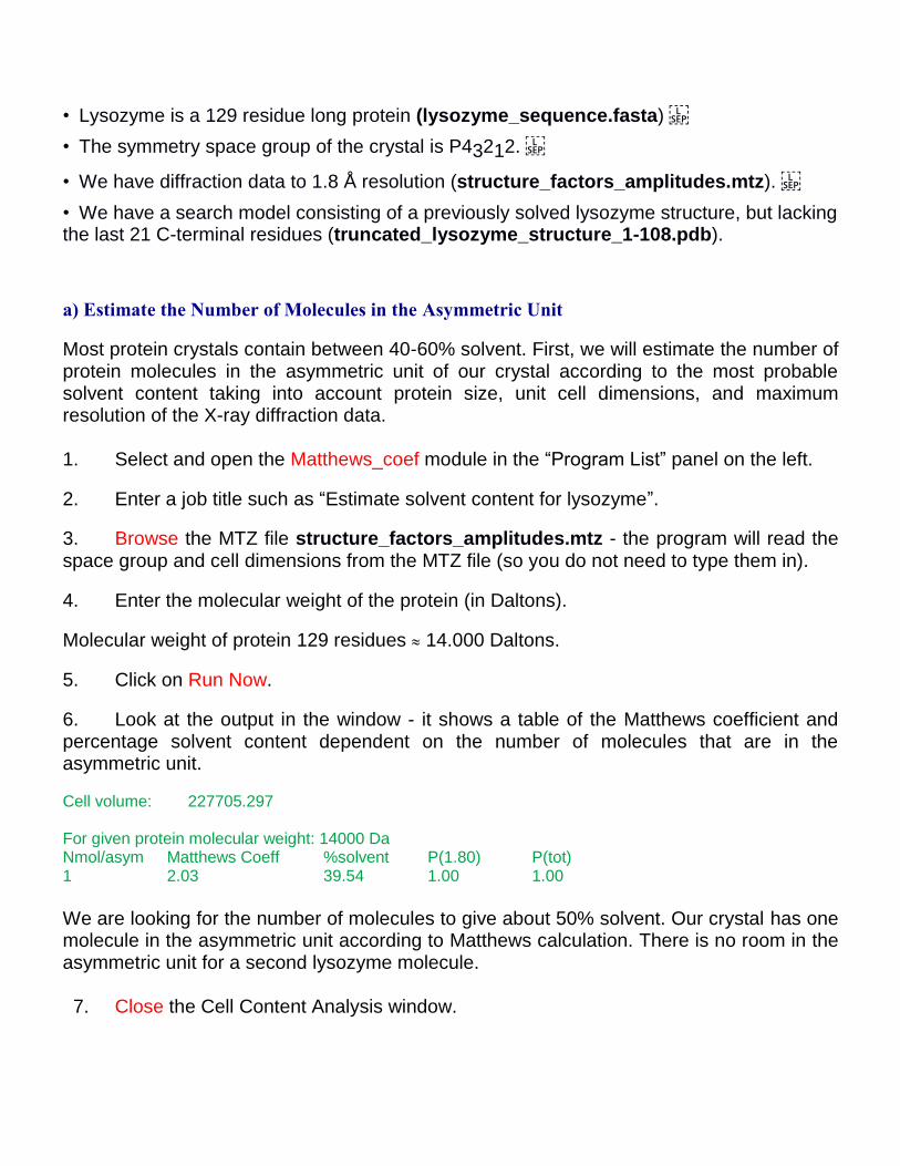
6. Look at the output in the window - it shows a table of the Matthews coefficient and percentage solvent content dependent on the number of molecules that are in the asymmetric unit.

Cell volume: 227705.297 For given protein molecular weight: 14000 Da Nmol/asym Matthews Coeff %solvent P(1.80) P(tot) 1 2.03 39.54 1.00 1.00

We are looking for the number of molecules to give about 50% solvent. Our crystal has one molecule in the asymmetric unit according to Matthews calculation. There is no room in the asymmetric unit for a second lysozyme molecule. 7. Close the Cell Content Analysis window.

b) Molecular Replacement / Phaser

1. Select the Phaser MR in the “Program List” panel on the left in the main CCP4 window.

2. Enter a title in the “Job title” section for example “Molecular replacement – first attempt”

3. Leave “Mode for molecular replacement automated search” unchanged.

4. In the section “Define data”, press the Browse button and look for our observed structure factors file (structure_factors_amplitudes.mtz). Press OK.

5. In the section “Define ensembles (models)”, press the Browse button and look for the lysozyme truncated model file (truncated_lysozyme_structure_1-108.pdb). Press OK.Set the similarity to be sequence identity to 0.8. This means that our search model bears around 80% sequence identity with the full-length protein crystallized (keep in mind that this preliminary protein model lacks (on purpose) the last 21 C-terminal residues.

6. In the section “Define composition of the asymmetric unit”, press the Browse button and look for the lysozyme full-length sequence file (lysozyme_sequence.fasta). Press OK.If you want, you can click on the View button located to the right, and a new window will pop up showing the one-letter sequence code of the full-length protein.

7. In the section “Search parameters”, go to “Perform search using” and click on ensemble1.

Here we indicate which model we want to use for the molecular replacement search.

8. Click Run -> Run Now. The program will run for some seconds. Wait for the “FINISHED”

label on the top of the main CCP4 window.

Output files

.pdb file Lysozyme_2.1.pdb By default, Phaser produces a .pdb file for only the top solution found. This corresponds to

our search model (C-terminally truncated lysozyme properly placed in the asymmetric unit of our crystal structure).

.mtz file Lysozyme_2.1.mtz

The .mtz file produced by the automated search contains the data from the input .mtz file, as

well as new columns, including information to calculate the electron density map.

.sol file Lysozyme_2.1.sol Potential solutions are described in a .sol file. Each potential solution starts with a SOLU SET line, and subsequent SOLU 6DIM lines describe the orientations and positions of molecules making up the solution.

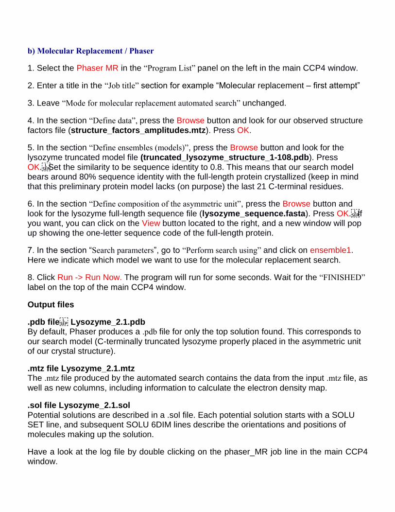
Have a look at the log file by double clicking on the phaser_MR job line in the main CCP4 window.

The log file ** Steps: ** Cell Content Analysis ** Anisotropy correction ** Translational NCS correction ** Rotation Function ** Translation Function ** Packing ** Refinement ** Final Refinement (if data higher resolution than search resolution) Space-Group Name (Hall Symbol): P 43 21 2 ( P 4nw 2abw) Space-Group Number: 96 Unit Cell: 78.18 78.18 37.25 90.00 90.00 90.00 Cell Content Analysis Composition is of type: PROTEIN MW to which Matthews applies: 14322 Resolution for Matthews calculation: 1.80 Z MW VM % solvent rel. freq. 1 14322 1.99 38.11 1.000 <== most probable Z is the number of multiples of the total composition In most cases the most probable Z value should be 1 If it is not 1, you may need to consider other compositions Rotation Function Two scores are given for each orientation: the log-likelihood-gain (LLG) and the Z-score. The LLG indicates how much better the data can be predicted from the oriented model than from a random-atom model. There are two things you can learn from the LLG. First, it should be positive, otherwise your oriented model is worse than a random-atom model! If it is negative, something is wrong: your model might be much worse than expected (e.g. there is an unmodelled hinge motion between domains, or the fold is less well preserved than one expects from the sequence identity), or it is less complete than expected (e.g. there is a second copy in the asymmetric unit). Second, the absolute value of the LLG can be used to compare the quality of different models against the same data. If you are testing different choices of model, the best one should give the highest LLG. If you are adding new information to the model (e.g. translation information for an oriented model, second subunit), the LLG should increase at each step. The Z-score is computed as the LLG minus the mean LLG for a random sample of orientations, divided by the RMS deviation of a random sample of LLG values from the mean. In other words, it tells you the number of standard deviations above the mean for a particular LLG score. Z-scores for correct orientations can be relatively low in difficult cases (e.g. less than 4), but a Z-score above 5 is usually correct. In addition, some sense of the significance of the solution can be gained from the number of orientations accepted for a subsequent translation search. If there is only one orientation above 75% of the maximum, then there is a very good chance it is correct. ****************************************************************************************** *** Phaser Module: MOLECULAR REPLACEMENT ROTATION FUNCTION 2.7.17 ***

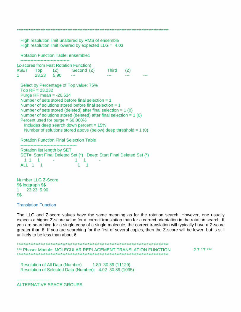
****************************************************************************************** High resolution limit unaltered by RMS of ensemble High resolution limit lowered by expected LLG = 4.03 Rotation Function Table: ensemble1 ---------------------------------- (Z-scores from Fast Rotation Function) #SET Top (Z) Second (Z) Third (Z) 1 23.23 5.90 --- --- --- --- Select by Percentage of Top value: 75% Top RF = 23.232 Purge RF mean = -26.534 Number of sets stored before final selection = 1 Number of solutions stored before final selection = 1 Number of sets stored (deleted) after final selection = 1 (0) Number of solutions stored (deleted) after final selection = 1 (0) Percent used for purge = 60.000% Includes deep search down percent = 15% Number of solutions stored above (below) deep threshold = 1 (0) Rotation Function Final Selection Table --------------------------------------- Rotation list length by SET SET# Start Final Deleted Set (*) Deep: Start Final Deleted Set (*) 1 1 1 - 1 1 - ALL 1 1 1 1 Number LLG Z-Score $$ loggraph $$ 1 23.23 5.90 $$ Translation Function The LLG and Z-score values have the same meaning as for the rotation search. However, one usually expects a higher Z-score value for a correct translation than for a correct orientation in the rotation search. If you are searching for a single copy of a single molecule, the correct translation will typically have a Z-score greater than 8. If you are searching for the first of several copies, then the Z-score will be lower, but is still unlikely to be less than about 6. ****************************************************************************************** *** Phaser Module: MOLECULAR REPLACEMENT TRANSLATION FUNCTION 2.7.17 *** ****************************************************************************************** Resolution of All Data (Number): 1.80 30.89 (11129) Resolution of Selected Data (Number): 4.02 30.89 (1095) ------------------------ ALTERNATIVE SPACE GROUPS

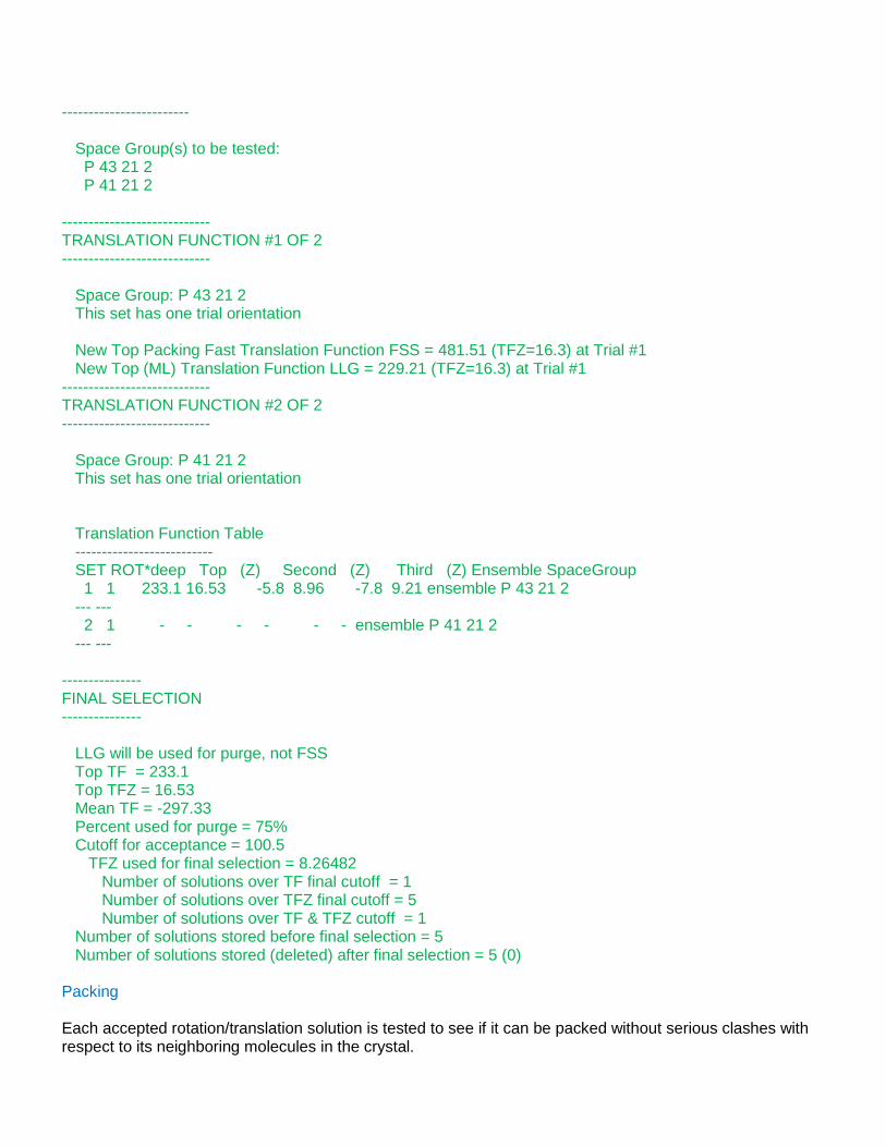
------------------------ Space Group(s) to be tested: P 43 21 2 P 41 21 2 ---------------------------- TRANSLATION FUNCTION #1 OF 2 ---------------------------- Space Group: P 43 21 2 This set has one trial orientation New Top Packing Fast Translation Function FSS = 481.51 (TFZ=16.3) at Trial #1 New Top (ML) Translation Function LLG = 229.21 (TFZ=16.3) at Trial #1 ---------------------------- TRANSLATION FUNCTION #2 OF 2 ---------------------------- Space Group: P 41 21 2 This set has one trial orientation Translation Function Table -------------------------- SET ROT*deep Top (Z) Second (Z) Third (Z) Ensemble SpaceGroup 1 1 233.1 16.53 -5.8 8.96 -7.8 9.21 ensemble P 43 21 2 --- --- 2 1 - - - - - - ensemble P 41 21 2 --- --- --------------- FINAL SELECTION --------------- LLG will be used for purge, not FSS Top TF = 233.1 Top TFZ = 16.53 Mean TF = -297.33 Percent used for purge = 75% Cutoff for acceptance = 100.5 TFZ used for final selection = 8.26482 Number of solutions over TF final cutoff = 1 Number of solutions over TFZ final cutoff = 5 Number of solutions over TF & TFZ cutoff = 1 Number of solutions stored before final selection = 5 Number of solutions stored (deleted) after final selection = 5 (0) Packing Each accepted rotation/translation solution is tested to see if it can be packed without serious clashes with respect to its neighboring molecules in the crystal.

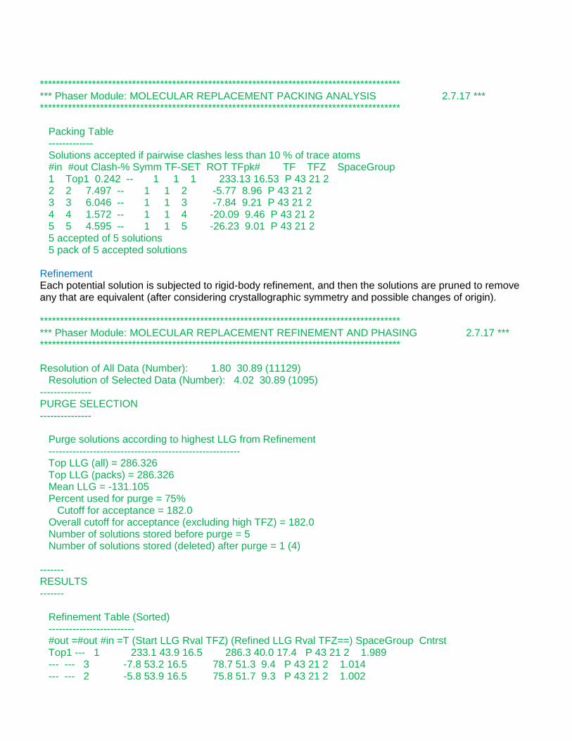
****************************************************************************************** *** Phaser Module: MOLECULAR REPLACEMENT PACKING ANALYSIS 2.7.17 *** ****************************************************************************************** Packing Table ------------- Solutions accepted if pairwise clashes less than 10 % of trace atoms #in #out Clash-% Symm TF-SET ROT TFpk# TF TFZ SpaceGroup 1 Top1 0.242 -- 1 1 1 233.13 16.53 P 43 21 2 2 2 7.497 -- 1 1 2 -5.77 8.96 P 43 21 2 3 3 6.046 -- 1 1 3 -7.84 9.21 P 43 21 2 4 4 1.572 -- 1 1 4 -20.09 9.46 P 43 21 2 5 5 4.595 -- 1 1 5 -26.23 9.01 P 43 21 2 5 accepted of 5 solutions 5 pack of 5 accepted solutions Refinement Each potential solution is subjected to rigid-body refinement, and then the solutions are pruned to remove any that are equivalent (after considering crystallographic symmetry and possible changes of origin). ****************************************************************************************** *** Phaser Module: MOLECULAR REPLACEMENT REFINEMENT AND PHASING 2.7.17 *** ****************************************************************************************** Resolution of All Data (Number): 1.80 30.89 (11129) Resolution of Selected Data (Number): 4.02 30.89 (1095) --------------- PURGE SELECTION --------------- Purge solutions according to highest LLG from Refinement -------------------------------------------------------- Top LLG (all) = 286.326 Top LLG (packs) = 286.326 Mean LLG = -131.105 Percent used for purge = 75% Cutoff for acceptance = 182.0 Overall cutoff for acceptance (excluding high TFZ) = 182.0 Number of solutions stored before purge = 5 Number of solutions stored (deleted) after purge = 1 (4) ------- RESULTS ------- Refinement Table (Sorted) ------------------------- #out =#out #in =T (Start LLG Rval TFZ) (Refined LLG Rval TFZ==) SpaceGroup Cntrst Top1 --- 1 233.1 43.9 16.5 286.3 40.0 17.4 P 43 21 2 1.989 --- --- 3 -7.8 53.2 16.5 78.7 51.3 9.4 P 43 21 2 1.014 --- --- 2 -5.8 53.9 16.5 75.8 51.7 9.3 P 43 21 2 1.002

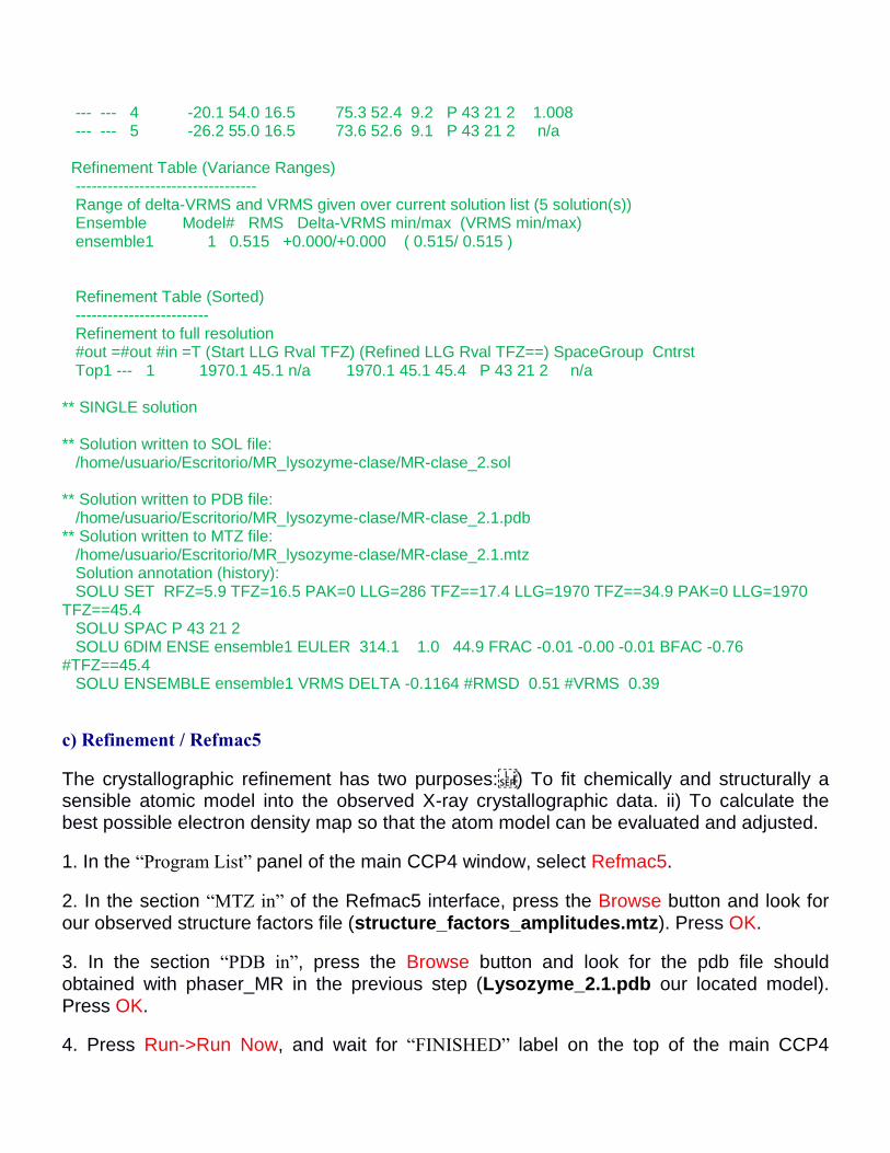
--- --- 4 -20.1 54.0 16.5 75.3 52.4 9.2 P 43 21 2 1.008 --- --- 5 -26.2 55.0 16.5 73.6 52.6 9.1 P 43 21 2 n/a Refinement Table (Variance Ranges) ---------------------------------- Range of delta-VRMS and VRMS given over current solution list (5 solution(s)) Ensemble Model# RMS Delta-VRMS min/max (VRMS min/max) ensemble1 1 0.515 +0.000/+0.000 ( 0.515/ 0.515 ) Refinement Table (Sorted) ------------------------- Refinement to full resolution #out =#out #in =T (Start LLG Rval TFZ) (Refined LLG Rval TFZ==) SpaceGroup Cntrst Top1 --- 1 1970.1 45.1 n/a 1970.1 45.1 45.4 P 43 21 2 n/a ** SINGLE solution ** Solution written to SOL file: /home/usuario/Escritorio/MR_lysozyme-clase/MR-clase_2.sol ** Solution written to PDB file: /home/usuario/Escritorio/MR_lysozyme-clase/MR-clase_2.1.pdb ** Solution written to MTZ file: /home/usuario/Escritorio/MR_lysozyme-clase/MR-clase_2.1.mtz Solution annotation (history): SOLU SET RFZ=5.9 TFZ=16.5 PAK=0 LLG=286 TFZ==17.4 LLG=1970 TFZ==34.9 PAK=0 LLG=1970 TFZ==45.4 SOLU SPAC P 43 21 2 SOLU 6DIM ENSE ensemble1 EULER 314.1 1.0 44.9 FRAC -0.01 -0.00 -0.01 BFAC -0.76 #TFZ==45.4 SOLU ENSEMBLE ensemble1 VRMS DELTA -0.1164 #RMSD 0.51 #VRMS 0.39

c) Refinement / Refmac5

The crystallographic refinement has two purposes:i) To fit chemically and structurally a sensible atomic model into the observed X-ray crystallographic data. ii) To calculate the best possible electron density map so that the atom model can be evaluated and adjusted.

1. In the “Program List” panel of the main CCP4 window, select Refmac5.

2. In the section “MTZ in” of the Refmac5 interface, press the Browse button and look for our observed structure factors file (structure_factors_amplitudes.mtz). Press OK.

3. In the section “PDB in”, press the Browse button and look for the pdb file should obtained with phaser_MR in the previous step (Lysozyme_2.1.pdb our located model). Press OK.

4. Press Run->Run Now, and wait for “FINISHED” label on the top of the main CCP4

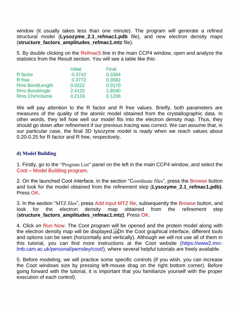
window (it usually takes less than one minute). The program will generate a refined structural model (Lysozyme_2.1_refmac1.pdb file), and new electron density maps (structure_factors_amplitudes_refmac1.mtz file).

5. By double clicking on the Refmac5 line in the main CCP4 window, open and analyze the statistics from the Result section. You will see a table like this:

Initial Final R factor 0.3742 0.3364 R free 0.3772 0.3582 Rms BondLength 0.0222 0.0170 Rms BondAngle 2.4125 1.8040 Rms ChirVolume 0.2118 0.1206

We will pay attention to the R factor and R free values. Briefly, both parameters are measures of the quality of the atomic model obtained from the crystallographic data. In other words, they tell how well our model fits into the electron density map. Thus, they should go down after refinement if our previous tracing was correct. We can assume that, in our particular case, the final 3D lysozyme model is ready when we reach values about 0.20-0.25 for R factor and R free, respectively.

d) Model Building

1. Firstly, go to the “Program List” panel on the left in the main CCP4 window, and select the

Coot – Model Building program.

2. On the launched Coot interface, in the section “Coordinate files”, press the Browse button and look for the model obtained from the refinement step (Lysozyme_2.1_refmac1.pdb). Press OK.

3. In the section “MTZ files”, press Add input MTZ file, subsequently the Browse button, and

look for the electron density map obtained from the refinement step (structure_factors_amplitudes_refmac1.mtz). Press OK.

4. Click on Run Now. The Coot program will be opened and the protein model along with the electron density map will be displayed.On the Coot graphical interface, different tools and options can be seen (horizontally and vertically). Although we will not use all of them in this tutorial, you can find more instructions at the Coot website (https://www2.mrc-lmb.cam.ac.uk/personal/pemsley/coot/), where several helpful tutorials are freely available.

5. Before modeling, we will practice some specific controls (if you wish, you can increase the Coot windows size by pressing left-mouse drag on the right bottom corner). Before going forward with the tutorial, it is important that you familiarize yourself with the proper execution of each control).

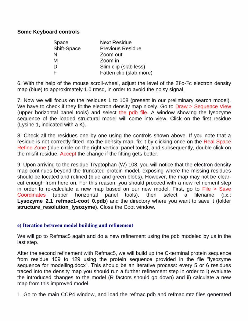
Some Keyboard controls

Space Shift-Space N M D F

Next Residue Previous Residue Zoom out Zoom in Slim clip (slab less) Fatten clip (slab more)

6. With the help of the mouse scroll-wheel, adjust the level of the 2Fo-Fc electron density

map (blue) to approximately 1.0 rmsd, in order to avoid the noisy signal.

7. Now we will focus on the residues 1 to 108 (present in our preliminary search model). We have to check if they fit the electron density map nicely. Go to Draw > Sequence View (upper horizontal panel tools) and select the pdb file. A window showing the lysozyme sequence of the loaded structural model will come into view. Click on the first residue (Lysine 1, indicated with a K).

8. Check all the residues one by one using the controls shown above. If you note that a residue is not correctly fitted into the density map, fix it by clicking once on the Real Space Refine Zone (blue circle on the right vertical panel tools), and subsequently, double click on the misfit residue. Accept the change if the fitting gets better.

9. Upon arriving to the residue Tryptophan (W) 108, you will notice that the electron density map continues beyond the truncated protein model, exposing where the missing residues should be located and refined (blue and green blobs). However, the map may not be clear-cut enough from here on. For this reason, you should proceed with a new refinement step in order to re-calculate a new map based on our new model. First, go to File > Save Coordinates (upper horizontal panel tools), then select a filename (i.e.: Lysozyme_2.1_refmac1-coot_0.pdb) and the directory where you want to save it (folder structure_resolution_lysozyme). Close the Coot window.

e) Iteration between model building and refinement

We will go to Refmac5 again and do a new refinement using the pdb modeled by us in the last step.

After the second refinement with Refmac5, we will build up the C-terminal protein sequence from residue 109 to 129 using the protein sequence provided in the file “lysozyme sequence for modelling.docx”. This should be an iterative process: every 5 or 6 residues traced into the density map you should run a further refinement step in order to i) evaluate the introduced changes to the model (R factors should go down) and ii) calculate a new map from this improved model.

1. Go to the main CCP4 window, and load the refmac.pdb and refmac.mtz files generated

by Refmac5 in Coot as specified in section d).

2. To trace the missing C-terminal residues, first go to the end of the protein chain using the tool Draw > Sequence View (upper horizontal panel tools).

3. Go to Add Residue (right vertical panel tools), and click (left mouse button) on the last residue modelled (which is Triptopfane 108 in this first tracing step). Accept the operation. If the added residue is located in a wrong place you can move it by pressing the left mouse button and dragging before accepting. In addition, if you wish to cancel any operation, press the arrowhead placed on the bottom of the right vertical panel tools, and select the option Undo.

4. By default, Coot adds an alanine residue at the C-terminus, therefore you have to change it for the correct one by clicking on Mutate & AutoFit (right vertical panel tools), and then on the added

alanine. After that, a windows showing all the 20 possible amino acids will appear, where we should select the correct one (in this case VAL, corresponding to the Valine 109 residue). Check that the added residue is well fitted into the density map. If not, proceed with the Real Space Refine Zone tool as specified in step 8. On the other hand, sometimes the bonds and angles of the added residue may suffer disorders, if so, use the Regularize Zone tool (white circle on the right vertical panel tools). Keep in mind that Real Space Refine Zone and Regularize Zone tools may be applied on a single or several residues, in this later case, click on the first residue of the region and make a second click on the last one.

5. Go on adding a few more residues [Alanine (A) 110, Tryptophan (W) 111, etc]. The electron density map may get worse (as specified above) and it might be difficult to place the following residue in the chain. At this moment, you should proceed with another refinement step again in order to recalculate a new map based on the latest model (as specified in section b) step 9).

6. Repeat this iterative process (model building and refinement) until tracing the complete sequence to the residue 129. After every refinement run, check that the residues that you had placed are correctly fitted into the electron density. Do not forget to save each latest traced model before proceeding with the next refinement step.

f) Last steps of model building (optional activity)

In the last step you can use the Validate section in Coot (upper horizontal panel tools) in order to check the regions of the model that require special attention after the rebuilding process (Ramachandran Plot, Geometry analysis, Density fit analysis, Rotamer analysis, etc).