Greening the Saskatchewan Grid

Brett David Dolter

A DISSERTATION SUBMITTED TO THE FACULTY OF GRADUATE STUDIES

IN PARTIAL FULFILLMENT OF THE REQUIREMENTS FOR THE DEGREE OF

DOCTOR OF PHILOSOPHY

GRADUATE PROGRAM IN THE FACULTY OF ENVIRONMENTAL STUDIES YORK UNIVERSITY

TORONTO, ON

December 2015

© Brett David Dolter, 2015

ii

Abstract

Saskatchewan is home to one of the most greenhouse gas (GHG) emissions intensive electricity sectors in Canada. To contribute to global efforts to mitigate climate change, and comply with Canadian coal-fired electricity regulations, the province must transform its electricity sector in the coming decades. This dissertation asks, what is the cost of reducing Saskatchewan’s electricity sector GHG emissions by 80% or more by 2050, using a mix of renewable electricity generating technologies? A renewable focused Greening the Saskatchewan Grid scenario is compared with a business-as-usual scenario and alternative pathways for reducing GHG emissions. Scenarios are selected using a linear programming model called the Saskatchewan Investment Model (SIM). The resulting scenarios are then tested using the ‘Will-It-Run-Electricity’ Model (WIRE) to understand whether a given electricity generation mix can adequately meet hourly electricity demand. Scenarios are compared using indicators such as electricity cost, GHG emissions, land impact, water impact, and radioactive waste, and sustainability criteria such as path dependence. It is found that a Greening the Grid scenario can reduce electricity sector GHG emissions to near zero levels by 2040. There is an added financial cost for taking this leadership path, but the cost of the Greening the Grid scenario becomes comparable to competing scenarios when an escalating carbon price is assumed. This dissertation also presents the results of a deliberative modelling exercise. Three workshops were held in Saskatchewan that brought together diverse participants interested in the future of the Saskatchewan electricity system. The goal of the workshops was to understand whether deliberation, supported by an interactive version of SIM, could encourage shared understanding of the barriers to and opportunities for expanding renewable energy in Saskatchewan. Workshop participants did not shift their positions to a great extent, except to find consensus that there are political and policy barriers to renewable energy expansion. This research contributes to the energy transitions literature by providing a case study of the costs and barriers faced when pursuing a renewable energy focused electricity system. It also contributes to the field of deliberative ecological economics and provides an example of an ecological economics approach to energy policy modelling.

iii

For my family

iv

Acknowledgements I would like to thank my supervisor Peter Victor for his wise counsel, encouragement, and kindness. The might of your intellect is matched with a warmth and good humour that has made my PhD journey, while challenging, at least happily so. Thank-you to my supervisory committee Ken Belcher, Ellie Perkins, and Mark Winfield for all of the work you put into this project, including countless hours reviewing research proposals and drafts of this document. It felt as if we were all rowing the boat together. Thank-you to Jennifer Fix for all your help workshop preparing, note transcribing, map making, and document stitching. Your support has made an impossible task possible and saved my sanity at all the right moments. A tremendous thank-you to everyone who participated in this research project, whether it was sitting down for an interview, attending a workshop, supplying data, or contributing in all three ways. This research is like the parable of stone soup; the contributions of research participants have made it much richer. Thanks especially to SaskPower for your openness and willingness to share information, and to Dr. Mark Bigland-Pritchard for the crucial hourly wind and solar data for Saskatchewan. Any errors and omissions are of course still the responsibility of the chef of this stone soup, myself. Lastly, I would like to acknowledge financial support from the Social Sciences and Humanities Research Council (SSHRC), and administrative support from York University’s Faculty of Environmental Studies.

v

Table of Contents

Pg.

Abstract ii

Dedication iii

Acknowledgements iv

Table of Contents v

List of Tables vi

List of Figures vii

1 – Introduction 1

2 – Towards an Ecological Economics Approach to Energy Policy Modelling 13

3 – A History of Saskatchewan’s Electricity System 37

4 – Renewable Options for A Low-Carbon Future 102

5 – Levelized Cost of Electricity Generation 134

6 – Electricity Demand Forecast and Energy Conservation Potential 159

7 – Scenarios for Greening the Saskatchewan Grid 181

8 – Scenario Impacts 220

9 – Deliberating Saskatchewan’s Electricity Future 267

10 – Conclusions and Next Steps 291

References 300

Appendix 5A – LCOE Methodology 337

Appendix 7A – Technical Documentation for the Saskatchewan Investment Model 347

Appendix 7B – Technical Documentation for the WIRE

(‘Will It Run Electricity’) Model 363

Appendix 8A – Cost of Service Model 383

Appendix 9A – Post-Workshop Survey 393

Appendix 9B – Workshop Script 397

Appendix 9C – Modelling Workbook 404

Appendix 9D – Pre-Workshop Survey 431

vi

List of Tables

Table 3-1 Cost of Electricity Generation in 1926 40 Table 3-2 Saskatchewan Power Commission Financial Conditions 49 Table 3-3 SaskPower Energy Conservation Programs 90 Table 3-4 Saskatchewan Electricity GHG Intensity 98 Table 4-1 Saskatchewan Hydroelectric Facilities (Year = 2015) 102 Table 4-2 Potential Hydroelectric Capacity 105 Table 4-3 Wind Power Projects in Saskatchewan 107 Table 4-4 Solar Photovoltaic in Cities Around the World 112 Table 4-5 Correlation of Hourly Wind Power Potential Across Saskatchewan

(January 1, 2013 to December 31, 2013) 123 Table 4-6 Saskatchewan’s Renewable Energy Potential 133 Table 5-1 EIA Learning Rates from 2019-2040 151 Table 5-2 Cost Assumptions for Saskatchewan Electricity Technologies 156 Table 6-1 Electricity Intensity Assumptions 163 Table 6-2 Peak Demand Savings Potential 166 Table 6-3 Electricity Conservation Potential 166 Table 6-4 Model Values Assumed for the Residential Sector 176 Table 6-5 Model Values Assumed for the Commercial Sector 176 Table 6-6 Model Values Assumed for the Industrial Sector 177 Table 7-1 White and Noble (2012) Scenario Outcomes in 2040 184 Table 7-2 Saskatchewan Coal-fired Generation Regulatory Impact 185 Table 8-1 Projected Costs 226 Table 8-2 Average Monthly Residential Electricity Bill 229 Table 8-3 Average Monthly Commercial Electricity Bill 232 Table 8-4 Electricity Intensive Industries in Canada (2011) 243 Table 8-5 Average Monthly Power Customer Electricity Bill 241 Table 8-6 Job Multiplier Factors 244 Table 8-7 Job-Years for Seven Scenarios 246 Table 8-8 GHGs Released to the Atmosphere by Scenario 248 Table 8-9 Cumulative Captured CO2 by Scenario 249 Table 8-10 Cumulative Storage Required for Captured CO2 250 Table 8-11 Land-use Factors for Wind and Solar Energy Installations 250 Table 8-12 Wind and Solar Land Use by Scenario (Sections) 251 Table 8-13 Water Impact Indicators 253 Table 8-14 Water Impact by Scenario (Gigalitres/yr) 253 Table 8-15 Water Impact by Scenario (thousands of Olympic sized pools/yr) 254 Table 8-16 High-Level Radioactive Waste 255 Table 8-17 Financial Cost Comparison 256 Table 8-18 Nuclear Decommissioning Costs 257 Table 8-19 Scenario Impacts in 2050 258 Table 9-1 Important Barriers to Renewable Energy (Pre-Workshop Survey) 276 Table 9-2 Maximum Percentage of Renewables Possible in Saskatchewan 282 Table 9-3 Coded Results of Opportunities and Barriers Exercise 284 Table 9-4 Importance of Barriers Pre- and Post-Workshop Survey Comparison 286

vii

List of Figures

Figure 1-1 Greenhouse Gas Intensity of Saskatchewan Electricity 5 Figure 1-2 Saskatchewan Electricity System 6 Figure 1-3 Electricity Capacity in Saskatchewan Minus Scheduled Retirements 7 Figure 1-4 Growth Trends in Saskatchewan 8 Figure 2-1 Participatory Modelling Plan 15 Figure 3-1 Average Personal Incomes Canada and Saskatchewan 1926-1950 43 Figure 3-2 Total Electricity Generation on the Saskatchewan Power Commission

System 1931-1948 44 Figure 3-3 SaskPower Electricity Generation 1952-1970 54 Figure 3-4 Cass-Beggs’ Hydro Plan for Saskatchewan 60 Figure 3-5 Bank Rate and 12-Month Canada All-Item CPI Percent Change 70 Figure 3-6 The Utility Death Spiral 79 Figure 3-7 Negative Learning-By-Doing in US and French Nuclear Power 85 Figure 3-8 Canada CPI Energy Index 12 month percentage change 86 Figure 3-9 ‘Penny Powers’ Promoting An Electric Oven-Range Appliance 88 Figure 3-10 Smart Grid Chronology 92 Figure 3-11 SaskPower Electricity Generation by Generation Type 97 Figure 3-12 History of the Saskatchewan Electricity System 101 Figure 4-1 Saskatchewan Hydroelectric Facilities Built and Proposed 103 Figure 4-2 Southern Saskatchewan Average Wind Speeds 106 Figure 4-3 Population Density in Southern Saskatchewan 110 Figure 4-4 Canada’s Renewable Energy Potential 111 Figure 4-5 Saskatchewan Solar Potential by Month in Four Select Cities 113 Figure 4-6 Approximate Temperature at the Base of the Sedimentary Section 115 Figure 4-7 Solar Thermal Using Parabolic Mirrors 116 Figure 4-8 Solar Thermal Using Heliostat Mirrors and a Central Tower 116 Figure 4-9 Hourly Wind Power Variability (January 28, 2013 – January 29, 2013) 122 Figure 4-10 Average Wind Power Output by Hour in 2013 124 Figure 4-11 Saskatchewan “Duck Chart” Showing Net Load With Solar-PV 125 Figure 4-12 Teaching the Duck to Fly 127 Figure 4-13 Annual Bright Sunshine Hours in Saskatoon 128 Figure 4-14 Hydroelectricity Capacity and Generation in Saskatchewan 129 Figure 4-15 Saskatchewan Hydroelectricity Generation and Streamflow in the

South Saskatchewan (S.SK) and North Saskatchewan (N.SK) Rivers 131 Figure 4-16 Drawdown of Underground Aquifers for Boundary Dam Cooling 132 Figure 5-1 Levelized Cost of Electricity from Electricity Cost Literature 137 Figure 5-2 Capital Costs of Electricity Generation Technologies 139 Figure 5-3 Sensitivity of Fossil Fuel LCOE to Carbon Pricing 142 Figure 5-4 Natural Gas Price at Louisiana’s Henry Hub 143 Figure 5-5 Sensitivity of Natural Gas Combined Cycle LCOE to Natural Gas Price 144 Figure 5-6 Saskatchewan Industrial Natural Gas Price Forecast 145 Figure 5-7 Sensitivity of Coal LCOE to Coal Prices 147 Figure 5-8 Falling Installed Cost of Solar Photovoltaics 148 Figure 5-9 Wind Power Transaction Prices in the United States (1997-2015) 149

viii

List of Figures cont. Figure 5-10 Levelized Cost of Electricity by Reference Source 157 Figure 6-1 Average Annual Electricity Use by a Residential Customer 160 Figure 6-2 Saskatchewan Electricity Demand Forecast (2015-2055) 161 Figure 6-3 Drivers of Electricity Demand 162 Figure 6-4 Estimated Sectoral Contributions to DSM 168 Figure 6-5 Power Demand on December 22nd, 2013 169 Figure 6-6 Residential DSM Program Costs (Year=2015) 171 Figure 6-7 Commercial DSM Program Costs (Year=2015) 173 Figure 6-8 Industrial DSM Program Costs (Year=2015) 173 Figure 7-1 Future Electricity Scenarios for Saskatchewan in 2040 183 Figure 7-2 SaskPower BAU to 2025 and Optimization to 2050 188 Figure 7-3 SaskPower Greenhouse Gas Emissions in Response to

Federal Regulation 189 Figure 7-4 Federal Regulation Equivalency Scenario 191 Figure 7-5 Average Electricity Prices Comparing Federal Regulation to

Equivalency 192 Figure 7-6 80% GHG Reduction: Scenario 1 – Interprovincial Approach 195 Figure 7-7 80% GHG Reduction Scenario 1 in Operation (December 2050) 197 Figure 7-8 Domestic 80% GHG Reduction: Scenario 2 – Nuclear Approach 198 Figure 7-9 80% GHG Reduction Scenario 2 in Operation (December 2050) 199 Figure 7-10 80% GHG Reduction: Scenario 3 – Carbon Capture Approach 200 Figure 7-11 The Cost of Achieving 80% Reduction in GHGs by 2050 201 Figure 7-12 80% GHG Reduction: Scenario 4 – Renewable Approach 203 Figure 7-13 80% GHG Reduction: Scenario 4 in Operation (December 2050) 204 Figure 7-14 Electricity Capacity in Domestic Renewable Energy Scenario 205 Figure 7-15 Peak Shaving Applied to Net Demand (December 7-9, 2050) 206 Figure 7-16 Solar Power Operation Domestic Renewable Scenario

(December 13-18, 2050) 207 Figure 7-17 80% GHG Reduction: Domestic Renewable Scenario in Operation

(June 2050) 208 Figure 7-18 Relative Cost of the Domestic Renewable Pathway 212 Figure 7-19 Greening the Grid Electricity Generation Mix 214 Figure 7-20 Scenario 4: 90% Renewable by 2050 Greenhouse Gas Emissions 215 Figure 7-21 Greening the Grid Greenhouse Gas Emissions 215 Figure 7-22 The Cost of Greening the Saskatchewan Grid 216 Figure 7-23 Cost Comparison With An Escalating Carbon Price 217 Figure 8-1 Residential Electricity Prices in Saskatchewan (cents/kWh) 228 Figure 8-2 Residential Rooftop Solar PV Achieving Grid Parity 230 Figure 8-3 Commercial Electricity Prices in Saskatchewan (cents/kWh) 231 Figure 8-4 Commercial Rooftop Solar PV Achieving Grid Parity 233 Figure 8-5 Feedback Loops in the Utility Sector 234 Figure 8-6 Large Power Customer Electricity Prices in Saskatchewan (cents/kWh) 237 Figure 8-7 Payments for Inputs in the Potash Sector (current dollars) 238

ix

List of Figures cont. Figure 8-8 Inside the Hitachi Manufacturing Plant 245 Figure 9-1 Responses to Question 1 of the Pre-Workshop Survey 272 Figure 9-2 Scenarios to Achieve Desired GHG Intensity (Pre-Workshop Survey) 274 Figure 9-3 Scenarios to Achieve High Level of Renewables

(Pre-Workshop Survey) 274 Figure 9-4 Scenario Building Screen in SIM 279 Figure 9-5 Workshop Scenario Outputs 280

1

Chapter 1 – Introduction

Introduction

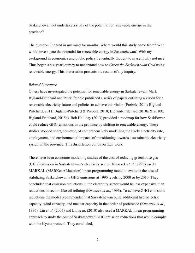
In the spring of 2009 the Government of Saskatchewan released a report by the

government-funded Uranium Development Partnership (UDP, 2009). The report set out

an ambitious expansion strategy for the Saskatchewan uranium mining industry, and

proposed that Saskatchewan construct “up to approximately 3000 MW of nuclear

capacity…to meet Saskatchewan’s power needs and capture export opportunities” (UDP,

2009: 55). Two months later former Deputy Premier Dan Perrins travelled around the

province seeking input from the people of Saskatchewan on the UDP proposals.

Thousands of citizens attended meetings expressing their opposition to the plan (Perrins,

2009). One of the strongest sentiments was that Saskatchewan had yet to explore other

low-carbon electricity pathways. Why, they asked, pursue dangerous nuclear power when

the province could instead pursue energy conservation and renewable energy from wind,

solar, biomass, and hydroelectricity?

I was working as a journalist that spring. When a friend called to ask if I would cover the

UDP consultation I agreed. The consultation would be the first province-wide discussion

of the uranium industry in a generation, and the first province-wide discussion of nuclear

power in the history of Saskatchewan. Scraping by with borrowed film equipment, and

sleeping on the couches of family, friends and acquaintances to conserve our limited

budget, we followed the Perrins consultation around the province. From the first meeting

in Yorkton, opposition to nuclear power was clear and strong. We arrived in Yorkton to

witness a local woman demand that Mr. Perrins allow her to present an alternative

perspective to the UDP. Perrins consented and so this concerned citizen stood at the front

of the room and warned of the dangers of nuclear power. She spoke of the long-lived

nuclear waste, the higher incidence of cancer in children who lived near nuclear power

plants in Germany, and the readily available renewable energy alternatives that could

provide Saskatchewan with the power it needed. This meeting was not unique. At each

stop on the trip we heard eloquent and well-researched arguments against nuclear power

and for renewable energy. A common question was: why does the Government of

2

Saskatchewan not undertake a study of the potential for renewable energy in the

province?

The question lingered in my mind for months. Where would this study come from? Who

would investigate the potential for renewable energy in Saskatchewan? With my

background in economics and public policy I eventually thought to myself, why not me?

Thus began a six-year journey to understand how to Green the Saskatchewan Grid using

renewable energy. This dissertation presents the results of my inquiry.

Related Literature

Others have investigated the potential for renewable energy in Saskatchewan. Mark

Bigland-Pritchard and Peter Prebble published a series of papers outlining a vision for a

renewable electricity future and policies to achieve this vision (Prebble, 2011; Bigland-

Pritchard, 2011; Bigland-Pritchard & Prebble, 2010; Bigland-Pritchard, 2010a & 2010b;

Bigland-Pritchard, 2015a). Bob Halliday (2013) provided a roadmap for how SaskPower

could reduce GHG emissions in the province by shifting to renewable energy. These

studies stopped short, however, of comprehensively modelling the likely electricity rate,

employment, and environmental impacts of transitioning towards a sustainable electricity

system in the province. This dissertation builds on their work.

There have been economic modelling studies of the cost of reducing greenhouse gas

(GHG) emission in Saskatchewan’s electricity sector. Kwaczek et al. (1996) used a

MARKAL (MARKet ALlocation) linear programming model to evaluate the cost of

stabilizing Saskatchewan’s GHG emissions at 1990 levels by 2000 or by 2010. They

concluded that emission reductions in the electricity sector would be less expensive than

reductions in sectors like oil refining (Kwaczek et al., 1996). To achieve GHG emissions

reductions the model recommended that Saskatchewan build additional hydroelectric

capacity, wind capacity, and nuclear capacity in that order of preference (Kwaczek et al.,

1996). Lin et al. (2005) and Lin et al. (2010) also used a MARKAL linear programming

approach to study the cost of Saskatchewan GHG emission reductions that would comply

with the Kyoto protocol. They concluded,

3

When Canada ratified the Kyoto protocol, the least-cost solution for

Saskatchewan in the absence of nuclear power, would be to phase out

coal-fired power generation plants and to replace them with lower

emission options, such as gas-fired, hydro, and wind-power technologies.

(Lin et al., 2010: 1601)

Lin et al. (2010) reported that nuclear power would achieve emissions reductions at a

lower price, if it were socially acceptable. They did not report the cost assumptions used

in their model.

While Kwaczek et al. (1996), Lin et al. (2005) and Lin et al. (2010) focused on short-

and medium-term GHG reductions in Saskatchewan to comply with a Kyoto-type

emission reduction target, they did not analyze the costs or opportunities to achieve more

ambitious long-term GHG reduction targets. These studies were also conducted on the

eve of large shifts in renewable energy costs. Solar costs have fallen substantially in

recent years, as has the cost of electricity storage (Barbose and Darghouth, 2015;

CitiGroup, 2015). Wind costs increased from 2000-2008, but have since fallen by 20-

40% (U.S. DoE, 2015). As the cost of generating and storing renewable energy falls, the

appeal of renewable energy for Saskatchewan increases. In this dissertation I explore the

potential for renewable energy to contribute to electricity sector GHG emission

reductions of 80% or greater by 2050. I compare the renewable energy pathway to other

scenarios for lowering GHG emissions in the Saskatchewan electricity sector.

Reports evaluating the potential for renewable energy have been conducted for Alberta

(Bell and Weis, 2009; Glave and Thibault, 2014) and Ontario (Weis and Partington,

2011; Weis et al., 2013). This dissertation provides a comparable report for

Saskatchewan. This research will also contribute to the energy transitions literature.

Jacobson and Delucchi (2011) and Delucchi and Jacobson (2011) outlined the potential

for renewable energy to provide all global energy needs by 2050. The research I have

conducted is a detailed look at how renewable energy could provide a substantial

4

proportion of electricity within a specific jurisdiction: Saskatchewan. This case study

approach offers insights into the sorts of real-world barriers that must be overcome if we

are to achieve an energy transition to renewables.

Several other studies of the Saskatchewan electricity system have been carried out in

recent years. White and Noble (2012) conducted a strategic environmental assessment to

rank pathways for reducing GHG emissions in the Saskatchewan electricity system. They

found that a renewable energy pathway was preferred by a group of expert participants,

and a nuclear focused pathway was ranked second. Richards et al. (2012) interviewed

eighteen individuals active in wind energy policy in Saskatchewan. They asked

participants whether the pace of wind expansion was fast enough, and also asked about

“barriers to expansion, and potential opportunities” (Richards et al., 2012: 3). Richards et

al. (2012) found that participants were divided in their assessments,

Participants could be divided into two major groups with opposing

viewpoints: those who felt that the current rate of wind energy

development was appropriate tended to identify technology as a major

barrier; those suggesting that current rate of expansion was insufficient

agreed that political barriers were amongst the most significant barriers.

(Richards et al., 2012: 4)

In my research I extended the work of Richards et al. (2012) by bringing Saskatchewan

electricity policy stakeholders together to discuss opportunities and barriers to renewables

in a deliberative workshop setting. I used these workshops to determine whether a shared

understanding could emerge between stakeholders with diverse positions, beliefs and

values.

Other studies of the Saskatchewan electricity sector include Richards et al. (2013) who

used Saskatchewan wind power as a case study for understanding barriers to effective

public policy communication. Linsay Martens (2015) analyzed Saskatchewan as a case

study of how First Nations could become involved in a renewable energy transition. I

5

hope that this dissertation can contribute to the growing literature on the cost and

potential for renewable energy in Saskatchewan.

Saskatchewan Context

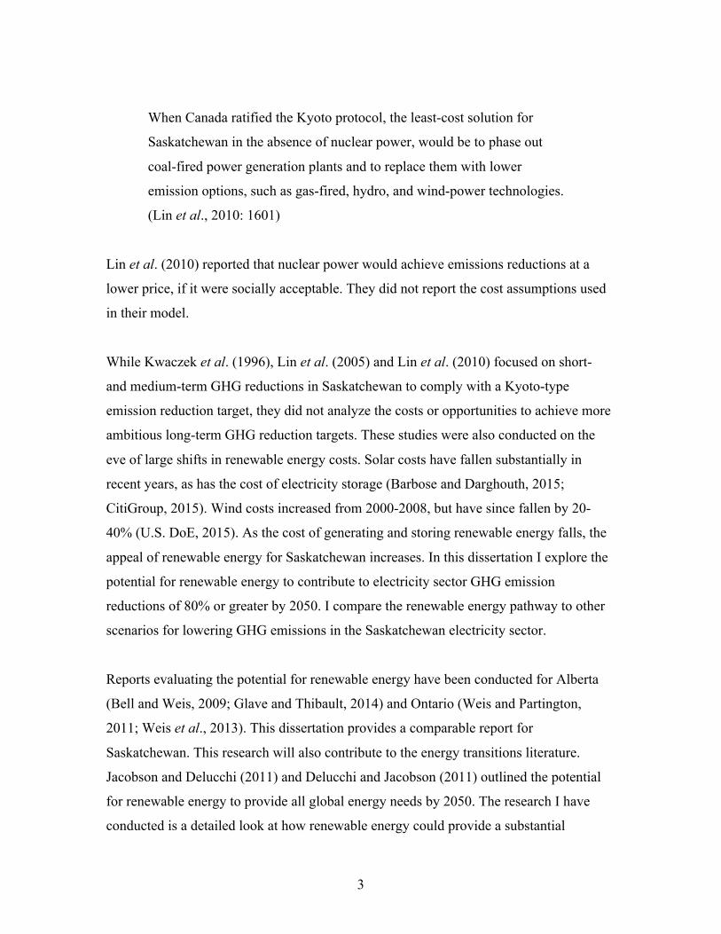
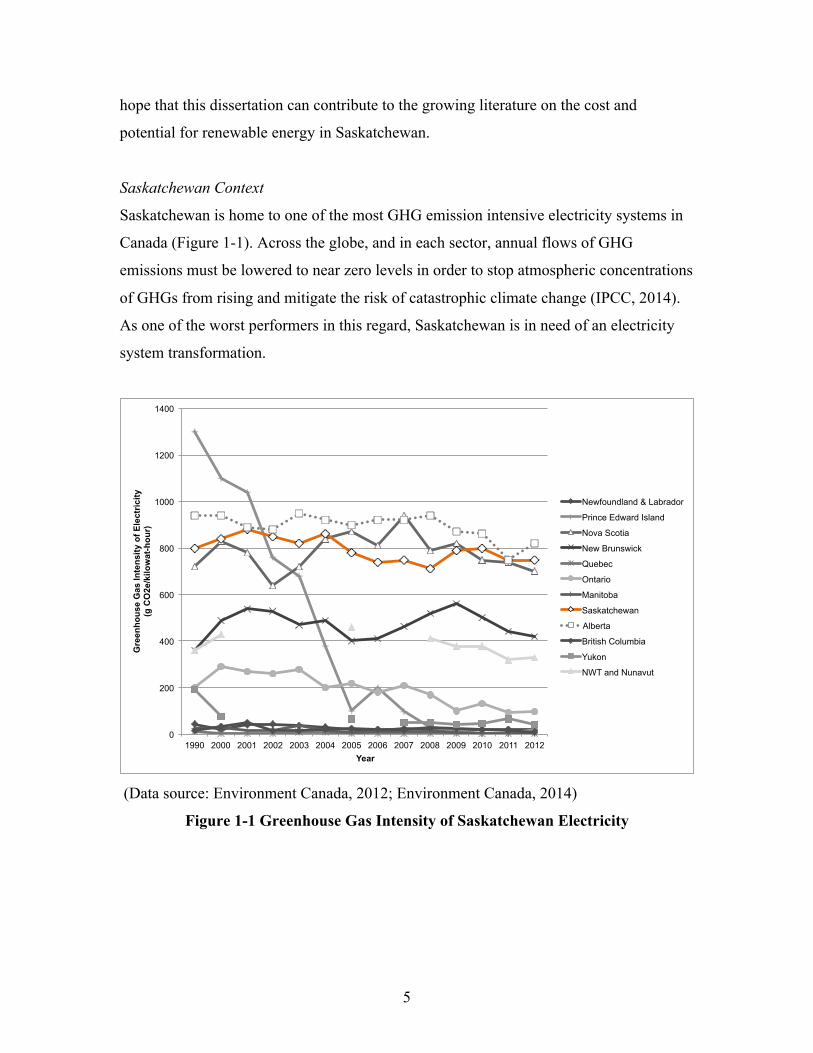
Saskatchewan is home to one of the most GHG emission intensive electricity systems in

Canada (Figure 1-1). Across the globe, and in each sector, annual flows of GHG

emissions must be lowered to near zero levels in order to stop atmospheric concentrations

of GHGs from rising and mitigate the risk of catastrophic climate change (IPCC, 2014).

As one of the worst performers in this regard, Saskatchewan is in need of an electricity

system transformation.

(Data source: Environment Canada, 2012; Environment Canada, 2014)

Figure 1-1 Greenhouse Gas Intensity of Saskatchewan Electricity

0

200

400

600

800

1000

1200

1400

1990 2000 2001 2002 2003 2004 2005 2006 2007 2008 2009 2010 2011 2012

Gre

enho

use

Gas

Inte

nsity

of E

lect

ricity

(g

CO

2e/k

ilow

at-h

our)

Year

Newfoundland & Labrador

Prince Edward Island

Nova Scotia

New Brunswick

Quebec

Ontario

Manitoba

Saskatchewan

Alberta

British Columbia

Yukon

NWT and Nunavut

6

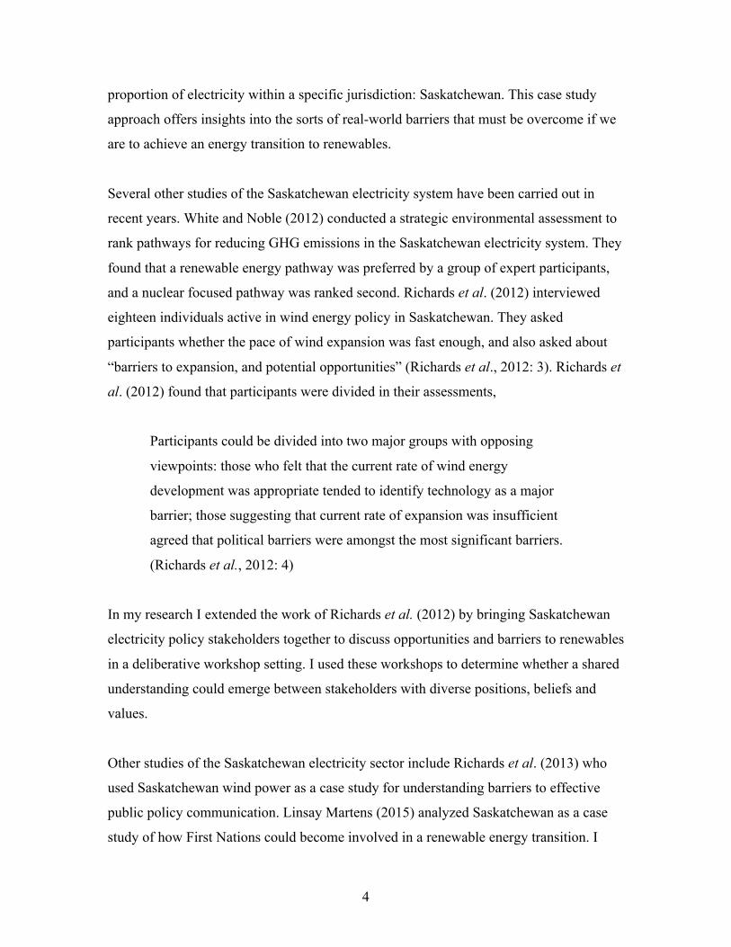
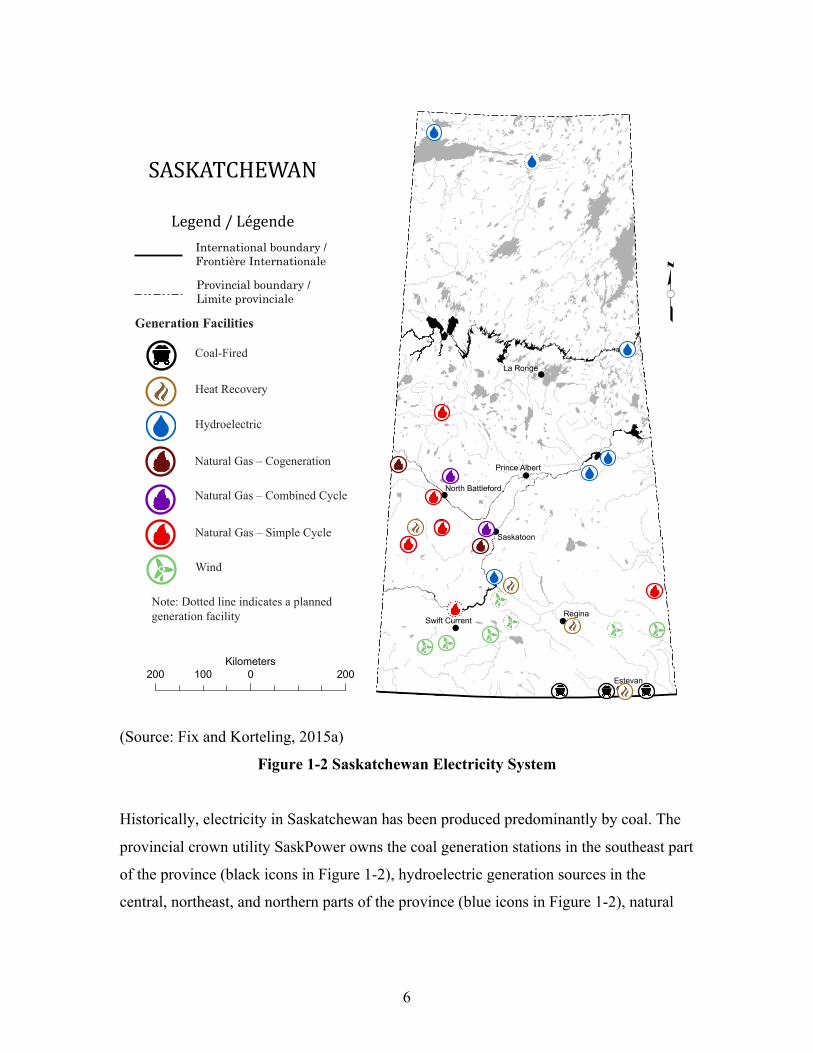
(Source: Fix and Korteling, 2015a)

Figure 1-2 Saskatchewan Electricity System

Historically, electricity in Saskatchewan has been produced predominantly by coal. The

provincial crown utility SaskPower owns the coal generation stations in the southeast part

of the province (black icons in Figure 1-2), hydroelectric generation sources in the

central, northeast, and northern parts of the province (blue icons in Figure 1-2), natural

!

!!

!

!

!

!

Regina

Estevan

La Ronge

Saskatoon

Prince Albert

Swift Current

North Battleford

tLegend / Légende

200 0 200100Kilometers

SASKATCHEWAN

International boundary / Frontière Internationale

Provincial boundary / Limite provinciale

Coal-Fired

Heat Recovery

Hydroelectric

Natural Gas – Cogeneration

Natural Gas – Combined Cycle

Natural Gas – Simple Cycle

Wind

Generation Facilities

Note: Dotted line indicates a planned

generation facility

!

!!

!

!

!

!

Regina

Estevan

La Ronge

Saskatoon

Prince Albert

Swift Current

North Battleford

tLegend / Légende

200 0 200100Kilometers

SASKATCHEWAN

International boundary / Frontière Internationale

Provincial boundary / Limite provinciale

7

gas facilities in the western part of the province (red and purple icons in Figure 1-2), and

wind installations in the southwest (green icons in Figure 1-2).

SaskPower also purchases electricity from independent (i.e. private) power producers,

including wind farms, natural gas plants (e.g. the Cory natural gas cogeneration facility

operated by Potash Corporation of Saskatchewan, the dark maroon flame southwest of

Saskatoon Figure 1-2), and heat recovery power-production installations owned and

operated by the pipeline industry (light brown icons in Figure 1-2).

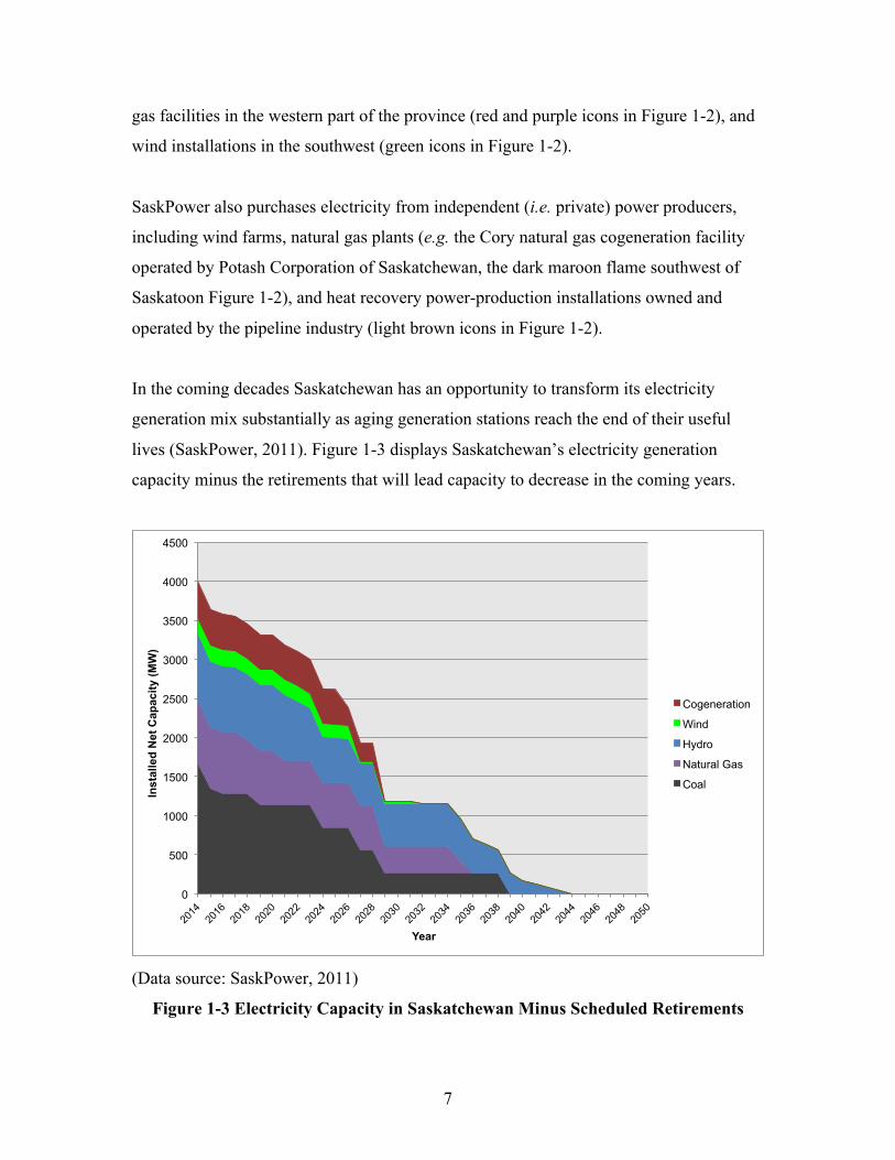
In the coming decades Saskatchewan has an opportunity to transform its electricity

generation mix substantially as aging generation stations reach the end of their useful

lives (SaskPower, 2011). Figure 1-3 displays Saskatchewan’s electricity generation

capacity minus the retirements that will lead capacity to decrease in the coming years.

(Data source: SaskPower, 2011)

Figure 1-3 Electricity Capacity in Saskatchewan Minus Scheduled Retirements

0

500

1000

1500

2000

2500

3000

3500

4000

4500

2014

20

16

2018

20

20

2022

20

24

2026

20

28

2030

20

32

2034

20

36

2038

20

40

2042

20

44

2046

20

48

2050

Inst

alle

d N

et C

apac

ity (M

W)

Year

Cogeneration

Wind

Hydro

Natural Gas

Coal

8

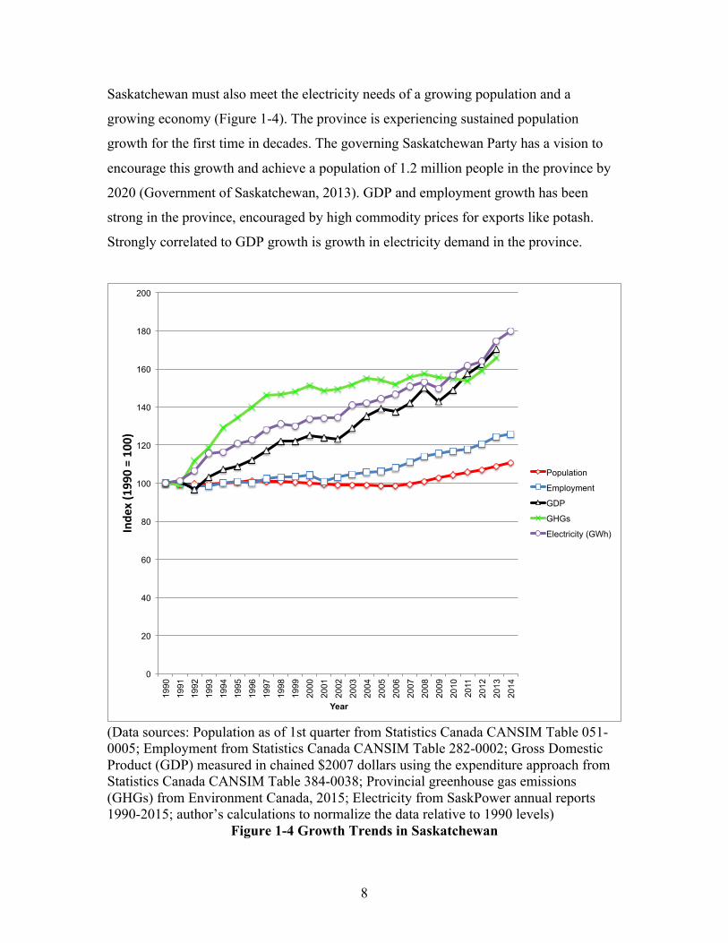
Saskatchewan must also meet the electricity needs of a growing population and a

growing economy (Figure 1-4). The province is experiencing sustained population

growth for the first time in decades. The governing Saskatchewan Party has a vision to

encourage this growth and achieve a population of 1.2 million people in the province by

2020 (Government of Saskatchewan, 2013). GDP and employment growth has been

strong in the province, encouraged by high commodity prices for exports like potash.

Strongly correlated to GDP growth is growth in electricity demand in the province.

(Data sources: Population as of 1st quarter from Statistics Canada CANSIM Table 051-0005; Employment from Statistics Canada CANSIM Table 282-0002; Gross Domestic Product (GDP) measured in chained $2007 dollars using the expenditure approach from Statistics Canada CANSIM Table 384-0038; Provincial greenhouse gas emissions (GHGs) from Environment Canada, 2015; Electricity from SaskPower annual reports 1990-2015; author’s calculations to normalize the data relative to 1990 levels)

Figure 1-4 Growth Trends in Saskatchewan

0

20

40

60

80

100

120

140

160

180

200

1990

19

91

1992

19

93

1994

19

95

1996

19

97

1998

19

99

2000

20

01

2002

20

03

2004

20

05

2006

20

07

2008

20

09

2010

20

11

2012

20

13

2014

Inde

x(1990=100)

Year

Population

Employment

GDP

GHGs

Electricity (GWh)

9

As SaskPower works to supply growing demand, while coping with aging infrastructure,

it can be assured that Saskatchewan’s future electricity mix will not look like the past.

The Government of Canada has introduced regulations that specify that Saskatchewan

must either retire its coal-fired electricity plants or retrofit them with carbon capture and

storage (CCS) technology to ensure they achieve a GHG intensity of no more than 420

grams CO2 per kilowatt-hour (kWh) (CEPA, 2012). To comply with the regulations all

but one coal-fired power plant must be retired or retrofitted by 2029, creating an

opportunity for a large-scale shift away from conventional coal.

The Government of Saskatchewan has, however, made it a priority to find ways to “keep

coal in play” (Wall quoted in Zinchuk, 2014). Premier Brad Wall supports coal because it

provides jobs in the Estevan and Coronach areas and because Saskatchewan has a supply

of coal that could last another two to three hundred years and this provides a degree of

“energy independence” (Wall quoted in Zinchuk, 2014).

To “keep coal in play” SaskPower has tested the viability of CCS technology at the

Boundary Dam III station. This first-of-a-kind plant captures 90% of carbon dioxide

(CO2) before it leaves the smokestack. The CO2 is then sold to an oil company called

Cenovus for use in enhanced oil recovery. While CCS may prolong the life of

Saskatchewan’s coal-fired plants and coal industry, it has been criticized as a more

expensive and less sustainable way of reducing emissions than renewables, especially

wind (Glennie, 2015; Banks & Bigland-Pritchard, 2015).

Saskatchewan has a strong wind resource and one of the best solar resources in Canada

(see Chapter 4). The electricity system is poised for a great transition. Despite its small

population Saskatchewan has shown a willingness to be a laboratory for sustainable

electricity policies. With a concerted effort Saskatchewan could become the first

jurisdiction to meet its energy needs by a combination of wind, water and solar power

(Jacobson and Delucchi, 2011 and Delucchi and Jacobson, 2011). In this dissertation I

explore the potential to Green the Saskatchewan Grid.

10

Research Questions

I am guided by a central research question,

What is the cost of Greening the Saskatchewan Grid by lowering greenhouse gas (GHG)

emissions by 80% or more by 2050 with a renewable energy focused electricity pathway?

To allow comparison I also work to understand the costs of a business-as-usual electricity

scenario that keeps with SaskPower’s current supply plan, and other competing scenarios

for lowering GHG emissions. The central research question can be broken into several

smaller questions. I address each in the chapters to follow. The relevant chapters are

included in brackets after each question:

• Research Question #1 – What energy-environment-economy models are

commonly used to develop electricity scenarios and can I improve upon them?

(Chapter 2)

• Research Question #2 – What historical events have shaped the present

electricity system in Saskatchewan? (Chapter 3)

• Research Question #3 – What is the potential for renewable electricity

generation in Saskatchewan? (Chapter 4)

• Research Question #4 – How much do competing electricity generation

technologies cost in Saskatchewan? (Chapter 5)

• Research Question #5 – How will electricity demand in Saskatchewan change

between 2015 and 2050? (Chapter 6)

• Research Question #6 – What electricity generation and storage scenarios will

meet Saskatchewan’s annual energy needs out to 2050 while minimizing

electricity costs and meeting greenhouse gas emissions reduction targets?

(Chapter 7)

• Research Question #7 – Once a scenario is developed that meets projected

annual demand and achieves the desired objectives, how can I ensure that it can

also meet projected hourly demand? (Chapter 7)

11

On research question #7, in this dissertation I pay particular attention to scenarios that

feature renewable energy. In doing so, I am aware of the critique, oft heard in

Saskatchewan, that renewable energy is variable and so cannot provide a reliable supply

of electricity.1 With that critique in mind, I have worked to model the hourly operation of

each electricity scenario. This is a means of testing whether a given system can

adequately balance the variability of renewable energy. While this is not an engineering

study, I am interested in understanding the cost of balancing variable renewable

electricity generation using technologies like demand side management, electricity

storage, and hydroelectric power with reservoir storage. The operations modelling I have

conducted is a means of testing whether the level of electricity storage and generation

capacity included in each scenario is adequate. I discuss this modelling effort in greater

detail in Chapter 2, Chapter 7 and Appendix 7B.

• Research Question #8 – What are the projected electricity costs (Chapter 7) and

electricity rates (Chapter 8) in each electricity scenario?

• Research Question #9 – What are the projected greenhouse gas emissions

implications of each scenario? (Chapter 7 and Chapter 8)

• Research Question #10 – How does each scenario compare in regards to other

indicators that can be used in a sustainability assessment? (Chapter 8)

Perhaps my most ambitious research objective was to generate a shared understanding

amongst diverse stakeholders of the opportunities to expand renewable energy in

Saskatchewan and the barriers that prevent expansion. In particular I hoped to build a

shared understanding between SaskPower and environmental groups who have called for

1 In a recent news article, Mike Monea of SaskPower stated his views on this subject, “You need a lot of base power to support your renewables. You can’t really have 100 per cent renewables. If you do, you’re not going to have power all the time. That’s what people have difficulty understanding. Every time we have to replace a plant, we can’t just put up wind turbines. It doesn’t work. It’s too simplistic. It doesn’t work that way. Last Sunday we hit a peak (of power consumption) at 6 p.m., suppertime. We had one megawatt coming from our wind turbines. There was no wind blowing. What did we use? We used coal-fired plants for the baseload, so nobody had disruption in their power.” (Zinchuk, 2015)

12

a renewable energy future. To accomplish this research objective I convened three

workshops with diverse stakeholders to discuss the future of the Saskatchewan electricity

system with an emphasis on the potential for renewable energy to power the province. I

ask the following question of these workshops,

• Research Question #11 – Can a deliberative energy policy-modelling workshop

generate shared understanding amongst diverse participants on the potential for

renewable electricity to contribute to Saskatchewan’s electricity future? (Chapter

9)

By answering these research questions I hope to offer sound policy advice to SaskPower

and the Saskatchewan provincial government as to the relative merit of a pathway to

Green the Saskatchewan Grid. I also hope to inform broader efforts to assess the

sustainability of competing electricity scenarios in the province. Lastly, I hope to

empower citizen activists who asked for a detailed study into the potential for renewable

energy during the Perrins’ consultations of 2009 (Perrins, 2009). This dissertation

provides that study.

I now turn to the methods I have used to answer these questions.

13

Chapter 2 – Towards an Ecological Economics Approach to Energy Policy Analysis Introduction

In this dissertation I work to develop an ecological economics approach to energy policy

analysis. Ecological economics is a methodologically diverse “trans-discipline”

(Norgaard, 1989; Norgaard, 2007). Ecological economists are called to integrate

information from across the social and natural sciences, as well as the humanities

(Norgaard, 2007). This requires proficiency with conventional methods of economic

analysis, as well as openness to other ways of knowing. I use a diverse set of methods,

including participatory modelling, historical document analysis, linear programming, and

deliberative energy policy modelling to answer the research questions I outlined in

Chapter 1.

Participatory Modelling

To understand how to make my research useful to SaskPower, citizen activists, and

environmental non-governmental organizations I carried out a process of participatory

modelling. Participatory modelling is a form of interactive social research (Talwar et al.

2011) and embraces the ideal of sustainability as a process of democratic decision-

making (Robinson, 2004). Participatory modelling shares similarities to mediated

modelling (van den Belt, 2004) in that it relies on engagement to make a model

meaningful and useful to participants.

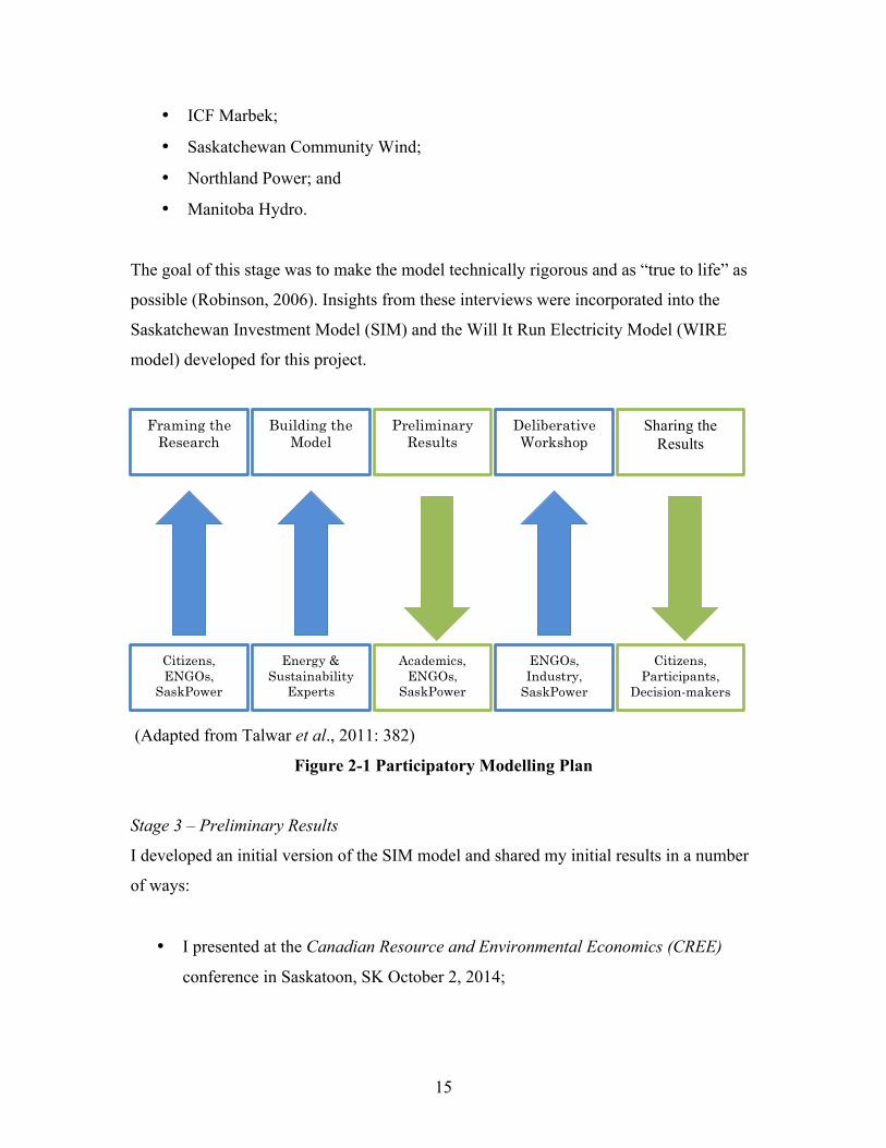
I carried out the process of participatory modelling in four stages (Figure 2-1). A fifth

stage of ‘sharing the results’ will follow the completion of my PhD program. The stages

proceeded as follows:

Stage 1 – Framing the Research

Engagement began in the early stages of the research process. I interviewed citizen

activists, environmental non-governmental organization representatives, technical

experts, and SaskPower staff and asked:

14

• What information gaps exist?

• What research questions should I strive to answer?

• What information would be useful for you to know?

What I heard from citizen activists and environmental non-government organizations

(ENGOs) was that they were looking for a detailed cost analysis of a renewable energy

future for Saskatchewan. Citizens and ENGO representatives were also interested in

understanding the employment impacts of a renewable energy scenario relative to a

business-as-usual scenario.

What I heard from SaskPower staff was that they were open to sharing their expertise

with me as I explored a renewable energy scenario. They also expressed concern over the

variability of renewable energy. This concern led me to ask, will a renewable focused

electricity system be capable of reliably supplying electricity to meet hourly electricity

demand?

Stage 2 – Building the Model

I conducted interviews with energy and sustainability experts to understand the technical

nuances of modelling the Saskatchewan electricity sector. These experts included

representatives from:

• SaskPower;

• Saskatoon Light and Power;

• Saskatchewan Eco-Network;

• Saskatchewan Environmental Society;

• Green Energy Project Saskatchewan;

• Summerhill Group;

• Saskatchewan Industrial Energy Consumers Association (SIECA);

• Saskatchewan Ministry of Economy;

• Saskatchewan Research Council;

• First Nations Power Authority;

15

• ICF Marbek;

• Saskatchewan Community Wind;

• Northland Power; and

• Manitoba Hydro.

The goal of this stage was to make the model technically rigorous and as “true to life” as

possible (Robinson, 2006). Insights from these interviews were incorporated into the

Saskatchewan Investment Model (SIM) and the Will It Run Electricity Model (WIRE

model) developed for this project.

(Adapted from Talwar et al., 2011: 382)

Figure 2-1 Participatory Modelling Plan

Stage 3 – Preliminary Results

I developed an initial version of the SIM model and shared my initial results in a number

of ways:

• I presented at the Canadian Resource and Environmental Economics (CREE)

conference in Saskatoon, SK October 2, 2014;

Framing the Research

Building the Model

Preliminary Results

Deliberative Workshop

Sharing the Results

Citizens, ENGOs,

SaskPower

Energy & Sustainability

Experts

Academics, ENGOs,

SaskPower

ENGOs, Industry,

SaskPower

Citizens, Participants,

Decision-makers

16

• I presented at the Ontario Network for Sustainable Energy Policy conference in

Waring House, Prince Edward County, ON April 28, 2015;

• I wrote a summary report outlining the initial results and shared the report with a

select group of participants I had interviewed. These participants were selected

based on their technical knowledge and level of interest in the project;

• I conducted follow-up interviews with a range of participants I had interviewed to

discuss my initial results.

Through this process I received useful feedback that helped me to improve the model.

This feedback included the following suggestions:

• Add Manitoba Hydro to the model;

• Add small, modular nuclear reactors as an investment option;

• Improve assumptions about the cost and potential of hydroelectric power in the

province;

• Use a multiplier to capture the cost premium paid to build thermal generation

(coal and natural gas fired facilities) in Saskatchewan. This cost premium is due

to factors such as a shortage of skilled labour in the province, which increases

project costs due to delays and higher payments to labour;

• Outline the employment impacts of the scenarios I created;

• Evaluate the impact of the federal government’s coal-fired regulations;

• Evaluate an ambitious greenhouse gas (GHG) emissions reduction scenario that

would include a coal phase-out by 2030.

Participants I spoke to also provided improved data for use in the modelling, including:

• The cost and potential of hydroelectric power in the province;

• Ramp rates for electricity generation technologies in Saskatchewan;

• Additional cost data for electricity generation technologies.

I incorporated this feedback into an improved version of SIM that included: updated cost

information; the addition of Manitoba Hydro and small, modular nuclear reactors as

generation technologies; and indicators such as jobs and water use. I used the enhanced

17

SIM model to evaluate the impact of the coal-fired regulations and an ambitious

Greening the Grid scenario (see Chapter 7).

Stage 4 – Deliberative Workshop

After improving the model using feedback from Stage 3, I ran three half-day workshops

of between six and eleven people to help generate scenarios for a sustainable electricity

system in Saskatchewan. Working from the mediated modelling philosophy I brought

together participants from a variety of interests and backgrounds to test whether a

deliberative modelling workshop could build consensus around the potential for

renewable energy to contribute to Saskatchewan’s electricity future (van den Belt, 2004).

These workshops were also a second chance for feedback on the model assumptions. The

outcomes of these workshops are outlined in detail in Chapter 9.

Stage 5 – Sharing the Results

After completion of the dissertation I plan to share the final results of this research

project with the participants who have provided input into the study. I then plan to

translate the dissertation into a format that can be easily communicated to decision-

makers and the broader Saskatchewan public. In this stage I hope to contribute to a

broader discussion of Saskatchewan’s electricity future. I also plan to continue offering

deliberative workshops and include a broader spectrum of participants.

Over the course of the participatory planning process I interviewed thirty-one individuals.

Twenty-one individuals participated in the deliberative modelling workshops, nine of

whom were also interviewed for the project. In total, forty-three individuals have

contributed their time and insights to this project. The process of involving stakeholders

in the modelling process has helped to ensure the relevance and accuracy of the

modelling work. I have heard from participants that they look forward to the final results.

It is my hope that the results of this analysis can contribute to a productive discussion of

Saskatchewan’s electricity future and the role of renewables in lowering Saskatchewan

greenhouse gas emissions.

18

History

The trans-disciplinary nature of ecological economics admits the value of case study and

qualitative research methods. We can learn from history. Political economist Harold

Innes taught us much about the Canadian economy by exploring the history of the fur

trade in this country (Innes, 1930). I studied the history of the Saskatchewan electricity

system through an analysis of SaskPower annual reports dating back to 1949, reports

from the Saskatchewan Power Commission dating from 1929-1949, books such as White

(1976) and Rediger (2004), and other assorted books and papers documenting the history

of electricity in the province.

An understanding of the historical roots of a problem can offer insights where context-

free economic analysis cannot. By studying the history of the Saskatchewan electricity

system I was able to understand why the crown utility focused their GHG reduction

efforts on expensive carbon capture and storage technology when an analysis of

economic costs would suggest pathways that could achieve the same GHG emission

reductions at a lower financial cost. Chapter 3 presents this historical analysis.

Energy-Environment-Economy Modelling

To evaluate the costs and greenhouse gas emissions of various scenarios for meeting

Saskatchewan’s electricity needs I built a suite of energy-environment economy models,

which includes the Saskatchewan Investment Model (SIM) and the Will It Run

Electricity (WIRE) model.

Economic models are a way of “disciplining our thinking” (Victor, 2015). They challenge

the modeller to understand the system well enough to describe it through numerical

representation. Models also help us to see relationships and outcomes that we might not

otherwise anticipate. Four energy-environment-economy models are frequently used to

analyze energy policy in Canada: Energy 2020, TIMES-Canada, CanESS, and CIMS. I

describe each in turn before outlining my own modelling approach.

19

Energy 2020 and TIM

Energy 2020 is a simulation model owned by the US private consulting firm Systematic

Solutions Inc. The model was created in 1981 to analyze regional energy and

environmental policy in the United States. It is now capable of analyzing regional energy

policy in fifty states, and each province and territory in Canada. (Amlin & Backus, 2014)

In Canada, the Energy 2020 model has been used by the National Energy Board (NEB) to

create their Canada’s Energy Futures reports (NEB, 2011; NEB, 2014a). In those reports

Energy 2020 is paired with the macroeconomic model TIM, which was created by the

private consulting firm Informetrica. TIM is “a detailed, dynamic econometric model of

the Canadian economy that provides the macroeconomic drivers for the modeling

framework” (NEB, 2014b). Macroeconomic forecasts in TIM are informed by projections

made by the private banks and government agencies such as the Federal Department of

Finance and the Bank of Canada (NEB, 2014b).

ENERGY 2020 and TIM communicate through changes in energy production, prices,

energy intensities, investments in energy industries, and various macroeconomic

parameters. The models run sequentially and iteratively over each year in the projection

period. For each year, energy supply and demand outcomes from ENERGY 2020 are

read and processed by TIM. TIM incorporates the energy information into a new

macroeconomic projection for the year. The new macroeconomic data is then returned to

ENERGY 2020 to create a new energy projection for the next iteration. More

specifically, ENERGY 2020 provides TIM with changes in energy production,

investments, energy intensity, and prices. TIM provides changes in gross domestic

product (GDP), gross output, housing, inflation, the Canada-U.S. exchange rate, floor

space, and population. (NEB, 2014b: 3-4)

The macroeconomic capabilities of the Energy 2020-TIM combination have made the

NEB projections the preferred macroeconomic forecast of Canadian energy policy

modelers. For example, the TIMES-Canada model uses the economic and demographic

forecasts from the NEB Canada’s Energy Futures reports – developed using the

20

Energy2020-TIM combination – as an exogenous input (Vaillancourt et al., 2013).

Energy 2020 is also used for in-house policy analysis by Environment Canada and

NRCAN (Miller, 2014).

Energy 2020 is a capital stock turnover model. It models stocks of energy-using, energy-

converting, and energy-producing technologies in physical terms. The capital stock of

existing technologies ages and at the end of its useful life must be retired or retrofitted.

When demand for energy-related technologies exceeds supply, this demand must be met

with investment in new technologies. (Miller, 2014; NEB, 2014a)

Human behaviour in the model is represented by a multinomial logit (MNL) equation.

The multinomial logit equation indicates the probability that a consumer will choose a

specific technology represented in Energy 2020. Attributes like cost affect the probability

that a technology will be selected, but other attributes are relevant as well. For example,

consumers do not simply choose a stove with the lowest operating cost, “some people

choose gas stoves because they prefer to cook with them, not because of price

differentials” (SSI, 2014: 21). The multinomial logit equations are estimated using a

discrete choice econometric approach. (SSI, 2014; Miller, 2014)

The electricity module of Energy 2020 includes detailed information on existing

electricity generating units in Canada, including their capacity factors and scheduled

retirement dates (NEB, 2014b). Electricity demand is divided into two seasons (summer

and winter), and six time slices (peak, near peak, high intermediate, low intermediate,

high base load, and low base load) for a total of twelve representative time slices. A

linear programming approach is used to solve for the least cost method of meeting

electricity demand in each representative time slice. (Miller, 2014)

TIMES-Canada – GERAD

TIMES-Canada is a dynamic linear programming model developed by the Quebec-based

21

GERAD research institute.2 TIMES stands for “The Integrated MARKAL-EFOM

System” (Bahn et al., 2013). TIMES was developed as an extension and replacement of

the MARKAL, or MARKet ALlocation, linear programming model previously used by

GERAD. (Vaillancourt et al., 2013)

TIMES-Canada has been used to create an energy outlook for Canada to 2050

(Vaillancourt et al., 2013). It is one of two models being used in the Trottier Energy

Futures Project, which is a joint project between the David Suzuki Foundation and the

Canadian Academy of Engineering (Hoffman & McInnis, 2014).3 TIMES-Canada has

also been used to analyze scenarios for electric vehicle penetration in Canada (Bahn et

al., 2013). Applications of the new model will continue; the GERAD website indicates

that TIMES-Canada is now being applied to the study of pipeline expansion and future

scenarios for the oil industry.

TIMES-Canada is a bottom-up model with rich technological detail. Its database

“includes more than 5,000 specific technologies and 400 commodities in each province

and territory” (Vaillancourt et al., 2013: 4). The electricity segment of TIMES-Canada

explicitly models 3500 existing electricity plants in Canada.

TIMES-Canada runs from 2007 to 2050 in time steps of 1-2 years in the initial periods,

and five year time-steps in later periods. The model is divided into twelve “time-slices”

for each time-step representing combinations of daily electricity demand fluctuation (day,

night, peak); and seasonal demand variations (winter, spring, summer, fall). (Vaillancourt

et al., 2013)

Like Energy 2020, the TIMES-Canada model is driven by demand for energy services.

As Vaillancourt et al. (2013) write, “The TIMES-Canada model is driven by a set of 67

2 More information on the GERAD (Group for Research in Decision Analysis) can be found at: https://www.gerad.ca/en. 3 More information on the Trottier Energy Futures Project can be found at: http://www.trottierenergyfutures.ca.

22

end-use demands for energy services in five sectors: agriculture (AGR), commercial

(COM), industrial (IND), residential (RSD) and transportation (TRA)” (p. 4).

Future energy service demands result from exogenous projections of economic and

demographic trends that are sourced from the National Energy Board’s (2011) Canada’s

Energy Future outlook up to 2035 and extended to 2050 using a “regressive approach”

(Vaillancourt et al., 2013: 7). As discussed above, the National Energy Board (NEB)

projections are created using the Energy 2020 and TIM energy policy modeling

approach.

TIMES is also a capital stock turnover model. Stocks of technologies related to final

energy demand, secondary energy carriers, and primary energy supply are tracked in

TIMES-Canada. When existing technologies reach the end of their useful lives, or

demands for energy services grow, new technologies compete to provide the required

end-use demand service, energy conversion service, and to supply primary energy.

For example, in Bahn et al., (2013) an array of conventional, hybrid, and electric vehicles

is available in the model to meet demand for personal road transportation. These

automobile technologies compete, “based on lifecycle costs, which are calculated using

capital, operation and maintenance and fuel costs” (Bahn et al., 2013: 596). Through an

optimization routine, TIMES-Canada selects the lowest cost means of meeting the

required demand over the time horizon.

TIMES-Canada selects low-cost technologies through the process of maximizing “net

total surplus”, which is the “sum of producers’ and consumers’ surpluses” (Vaillancourt

et al., 2013: 3). Producer surplus is maximized by “minimizing the net total cost of the

energy system”, which includes investment costs, operation and maintenance costs, and

fuel costs (Vaillancourt et al., 2013: 3). Consumer surplus is maximized by minimizing

“welfare losses due to endogenous demand reductions” (Vaillancourt et al., 2013: 3).

This means that there is a penalty in the model for scenarios and technology choices that

raise the price of energy and reduce consumption of energy services. The objective

23

function combines the cost of the energy system to producers and the welfare losses to

consumers into one equation to be minimized.

The quantity of energy services demanded in TIMES-Canada is sensitive to price.

Elasticities define this price response. Generally, demand is exogenous in the “business-

as-usual” (BAU) run of the model, and becomes endogenous when scenarios are run to

test the impact of various policies (Vaillancourt et al., 2013). This price-driven demand

response provides macroeconomic feedback in the model.

TIMES-Canada is subject to the standard critiques of linear programming. Linear

programming models such as TIMES-Canada exhibit “penny-switching”, wherein the

optimization routine will favour one technology over another even if costs differ by mere

pennies (Jaccard et al., 2003). Market share constraints can be introduced to ensure that

individual technologies do not capture an entire market. However, these constraints

introduce a degree of arbitrariness into the model.

As a bottom-up model TIMES-Canada may fail to capture “intangible costs” such as the

sentiment that a new technology is risky because it is untried. Lacking these costs,

TIMES-Canada may be too optimistic about the costs of climate mitigation policies.

(Jaccard, 2002; Rivers & Jaccard, 2005)

To include consumer surplus in the objective function, TIMES-Canada models human

behaviour and preferences using a social welfare function. From an ecological economics

perspective the use of a social welfare function is problematic. This form of modelling

uses ‘RARE’ individuals to represent human behaviour. A RARE individual is a

homogenous Representative Agent acting with Rational Expectations to maximize utility

by maximizing consumption (King, 2015). This caricature of human behaviour is

sometimes referred to as ‘homo economicus.’ While the representative agent makes

consumption decisions mathematically tractable in an optimization model, it is a

departure from the complex reality of human behaviour in the following ways:

24

• People are diverse and not well served by being treated as “homogenous globules

of desire” (Erickson quoting Thorstein Veblen, 2013);

• Preferences are not well-defined across all goods in a market, instead rationality is

bounded (Kahneman, 2003); this means that rather than optimizing their

consumption decisions, people make decisions that “satisfice” (sufficiently satisfy

given the available information) (Simon, 1956);

• People are not solely self-interested and rapaciously working to maximize their

consumption of market goods, instead we are characterized by a mix of self-

regarding and other-regarding behaviour (Gintis, 2000).

Some scholars have called for ‘homo economicus’ to evolve into something more akin to

‘homo sapiens’ (Thaler, 2000). Others have argued that in a democracy it is better to ask

people what they want, and let them deliberate and debate in a public forum, rather than

to simply assume their desires and fold the assumptions into an economic model

(Norgaard, 2007). In the case of lowering greenhouse gas emissions in the electricity

sector, we could ask if people are willing to pay more for electricity in order to stabilize

the climate. Discussion of such trade-offs is inherently political and is influenced by the

values and identities of those engaged in the deliberation (Kahan et al., 2007). An

interactive approach to energy policy modelling, such as that applied in the CanESS

model, can be used to discuss those trade-offs and avoid the RARE assumption.

CanESS Model

The CanESS (Canadian Energy Systems Simulator) model was developed by Robert

Hoffman and Bert McInnis of ‘Whatif? Technologies’. The CanESS model is being used

in the Trottier Energy Futures Project for Canada along with the TIMES-Canada model

(Hoffman & McInnis, 2014). CanESS was used by the Pembina Institute to study the

future of electricity supply in Ontario (Weis & Partington, 2011). It has been used to

explore scenarios for alternative vehicles in Canada (Steenhof & McInnis, 2008). It has

also been used to create the Australian Stocks and Flow Framework (Turner et al., 2011).

The Canadian Energy Systems Analysis Research (CESAR) group – led by David

25

Layzell at the University of Calgary – is working to further develop CanESS for research

purposes.4

The prime objective of CanESS is to allow for the simulation of plausible scenarios for

Canada’s energy future. Plausible scenarios are those that respect fundamental physical

laws such as the conservation of energy and materials. CanESS models stocks and flows

using a physical accounting framework. This means that rather than focusing on the

economic value of human artifacts like cars and buildings, these are counted in physical

terms (number of cars, number of buildings, megawatts of electricity generation

capacity). Energy and material stocks and flows are also tracked in physical terms (e.g.

tonnes of coal). Physical stocks and flows must “obey the thermodynamic constraints of

conservation of mass and energy” (Turner et al., 2011: 1140).

CanESS avoids making any assumptions about human behaviour. The approach was

selected intentionally to remove “ideological bias…since the core represents largely

irrefutable accounting relationships reflecting mass balance” (Turner et al., 2011: 1147).

According to Hoffman and McInnis (2014), many energy policy models are built with the

embedded ideologies contained in economic theory. Hoffman (2012) is critical of the

RARE model of human behaviour arguing, “human behaviour is too diverse and complex

to be represented as an aggregate consumer agent” (p. 79).

Without behavioural assumptions CanESS cannot be used for least-cost optimization; the

model is not “closed” in the way that a linear programming model is closed. Instead it is a

descriptive model, “Open to the influence of different sets of values, i.e. not normative or

prescriptive, but more descriptive” (Turner et al., 2011: 1137).

Similar to a flight simulator, Hoffman and McInnis have designed CanESS to be highly

interactive. When a simulation is run, users are made aware of “tensions” in the model.

These tensions are instances when the model runs into “physically unfeasible or

problematic outcomes” (Turner et al., 2011: 1138). These tensions “must be resolved by

4 More information on CESAR can be found at: http://www.cesarnet.ca.

26

people interacting with the (model), similar to the flight simulator concept” (Turner et al.,

2011: 1138).

Through the process of resolving tensions CanESS becomes a learning tool. Like a

telescope, it is designed as an extension of the human nervous system. CanESS is meant

to help users better understand the long-term, systemic consequences of energy policy

choices. As such, Hoffman and McInnis (2014) borrow a concept from de Rosnay (1979)

and refer to CanESS as a kind of “macroscope.” (Hoffman & McInnis, 2014)

CanESS is designed to be used without reference to prices. For this reason it has been

critiqued by economists (Turner et al., 2011). However, Hoffman and McInnis (2014)

argue that price is a human-created institution and institutions can be changed. For

Hoffman and McInnis (2014) energy policy decision-making should begin with an

exploration of physically plausible scenarios for the future. Then decision-makers can

select a desirable scenario for the future. Only at the last stage, do decision-makers decide

on the policies and institutions required to support the desirable scenario. With this

approach energy policy models should never conclude that we “can’t afford” a physically

plausible scenario; if a scenario is physically plausible Hoffman & McInnis (2014) argue

that we should be able to design institutions, prices, and policies to support it. From an

energy policy modelling perspective this leaves something to be desired. CanESS lacks a

clear decision-rule for sorting between scenarios. The world of physically plausible

scenarios is wide and economic models are often tasked with recommending a favoured

scenario. We can ask, is it enough for a decision-maker to know a scenario is physically

plausible? Or will they expect more from a model and a modeller?

The results of CanESS simulations can be combined with financial cost information. The

modeling work conducted by the Pembina institute for Ontario’s electricity sector

identified “two plausible scenarios of Ontario’s electricity future” and reported on the

electricity price impacts of each (Weis & Partington, 2011: IV). The work of finding a

recommended cost-effective and plausible scenario occurs through iteration as the

modeller interacts with the CanESS model.

27

The CanESS scenarios for Ontario included rich detail on electricity demand: “hourly

load shape pattern is built up from a detailed end-use representation of electricity use

across all sectors of the economy”, and operational detail around dispatch rules for

supplying electricity (Weis & Partington, 2011: 10). The operational and investment

costs required to achieve each scenario were tracked and translated into electricity prices

over time for the two scenarios. The scenarios may not have been optimal, but were

physically plausible and robust.

CIMS-GEEM

The CIMS model was developed at Simon Fraser University (SFU) by Mark Jaccard,

John Nyboer, Chris Bataille, Nic Rivers and other students and faculty associated with

SFU’s Energy and Materials Research Group (EMRG). The model was built on code that

originated from the ISTUM model (built in the United States in the 1980s) and was

enhanced and extended at SFU throughout the past two decades (EMRG, 2014; Bataille,

1998).

CIMS has been used for consulting projects across Canada and the United States,

including analysis conducted for the National Round Table on the Environment and

Economy (e.g. NRTEE, 2009). CIMS is currently used as a consulting model by the firm

Navius and has been enhanced in recent years with the addition of a macroeconomic,

computable general equilibrium (CGE) sister model called GEEM.

CIMS is a “technology choice simulation model” (EMRG, 2014) that “simulates the

evolution of capital stocks over time” (Jaccard, 2009: 317). The model is billed as a

hybrid incorporating the technological detail of bottom-up modelling approaches (e.g.

linear programming) and the behavioural realism of top-down modeling (e.g. CGE

modeling) (Rivers & Jaccard, 2005; Jaccard, 2009).

On technological detail, CIMS contains “over 1000 technologies competing for market

share at hundreds of nodes throughout the economy” (Jaccard, 2009: 321). Data on the

technologies used by industry in Canada is enhanced by the close connection between

28

EMRG and the Canadian Industrial Energy End-Use Data and Analysis Centre

(CIEEDAC). John Nyboer, one of the architects of CIMS, heads up CIEEDAC.

Behavioural realism is represented in CIMS by a market share equation. Technologies

achieve market-share not based on cost alone, but also based on consumer preferences for

characteristics of the technology. These consumer preferences are represented by

discount rates and ‘intangible costs’ estimated from market data. For example, taking the

bus to work might be the least cost option for a commuter, but a preference for driving

may lead that person to take their car. The value of this preference must be worth at least

the difference between the cost of transit and the cost of driving. These cost differentials

are estimated from real world market data. (Rivers and Jaccard, 2005; Jaccard, 2009)

Like the Energy 2020 and TIMES-Canada models, CIMS is driven by exogenous demand

for energy-services. This demand is linked to economic and demographic forecasts.

CIMS has a macro-economic module containing elasticities that allow for demand to shift

when policies are introduced in the model. The integration of CIMS and the GEEM

computable general equilibrium (CGE) model now allows for further macroeconomic

feedback. GEEM is subject to the same critiques of ‘RARE’ modelling mentioned above.

(Rivers & Jaccard, 2005; Jaccard, 2009)

Model Comparison

The energy policy models reviewed above share the following common features:

• Capital Stock Turnover - Physical stocks of energy-using artifacts age, and must

be retired or repaired;

• Energy Service Demand – Demand for energy services such as lighting, heating,

and industrial processes drive the models. Technologies and energy sources

compete to supply these services.

The models differ in the following areas:

29

• Simulation or Optimization – TIMES-Canada is an optimization model and

Energy 2020 uses linear programming optimization for its electricity module, but

is otherwise a simulation model. CIMS and CanESS are simulation models;

• Human Behaviour – TIMES-Canada assumes cost-minimizing and welfare

maximizing behaviour, as does the GEEM CGE addition to CIMS. Energy 2020

and CIMS are built to allocate market share using logistic, probabilistic equations

estimated empirically. CanESS relies on user interaction rather than embedded

assumptions about human behaviour;

• Participatory modeling – Energy2020-TIM, TIMES-Canada, and CIMS-GEEM

are all expert models; that is they are designed and operated by modelling experts

with limited input from stakeholders. CanESS models are built through a

participatory process and user interactivity is an important feature;

• Technological detail – Models differ in the level of technological detail they

contain. While all of the models contain basic features of electricity generation

technologies such as capacity factors and fuel efficiencies, they differ in their

representation of the operation of an electricity system. TIMES-Canada represents

the operation of an electricity system using representative “time slices”. The

CanESS model for Ontario contains detailed hourly electricity demand and supply

information.

Towards An Ecological Economics Energy Modelling Approach

I have created a suite of energy-environment-economy models tailored to address my

specific research questions. When creating these models I worked to take the useful

elements from the models described above and improve upon their weaknesses. I

describe each model in turn.

The Saskatchewan Investment Model (SIM) is a linear-programming optimization model.

It is built to minimize the cost of meeting Saskatchewan electricity demand over the

course of 2015-2050. Investment decisions are made in five-year time-steps beginning in

2020. SIM is built with rich technological detail to describe the costs and operating

characteristics of the Saskatchewan electricity system, including the fuel use and

30

greenhouse gas emissions associated with each technology. It is a capital stock turnover

model in which generating units age and must be replaced or, in some instances,

retrofitted. Electricity demand is exogenous in the model and is calibrated to

SaskPower’s (2015) load forecast (see Chapter 6 for a detailed description of the

electricity forecast used). This means that the model does not include macroeconomic

feedback; energy demand does not respond to changes in price. SIM does, however,

include demand side management (DSM) as a supply option. If the costs of generating

electricity increase above those projected in the base case, then, in SIM, the utility puts

more effort into DSM to lower electricity demand. This behavior by the utility is a proxy

for price-induced reductions in electricity demand though it may not capture the full

amount. Otherwise SIM excludes a representation of demand-side human behaviour.

Instead, it represents the electricity system from the perspective of a rational system

planner responding to inelastic demand. In Saskatchewan the crown utility SaskPower

has a monopoly on electricity supply and a mandate to provide affordable electricity (i.e.

SaskPower does not seek out monopoly rents). This makes the electricity system

amenable to the assumption of a rational system planner; although in practice there are

significant socio-technical biases that influence SaskPower’s decision-making (see

Chapter 3 and Chapter 9). I do not address the issue of inelastic demand within SIM, but

instead discuss some of the implications of rising electricity prices in Chapter 8. I use

SIM to answer the research question, what electricity generation scenarios can lower

greenhouse gas emissions in Saskatchewan while minimizing financial cost? SIM is

described in detail in Technical Appendix 7A.

The Will-It-Run Electricity model (WIRE model) is an hourly operations model of the

Saskatchewan electricity system. The WIRE model includes real-world electricity

demand data, wind power production data, solar production data, and hydroelectric

seasonal capacity factors to provide a realistic picture of the variability of both electricity

demand and renewable energy production. Electricity storage capacity is modelled as a

means of smoothing the variability of renewable electricity production. Demand side

management is modelled through the option of ‘peak shifting’ demand three hours into

the future. Dispatchable electricity generation technologies (including electricity storage)

31

are called to meet electricity demand, but are constrained by ramp rates; this means that it

takes time for technologies to increase or decrease their output. The WIRE model is a

linear programming model that runs in the GAMS (General Algebraic Modelling

Software) modelling environment. A detailed description of WIRE is included in

Appendix 7B.

WIRE is designed to be used iteratively with SIM. Least-cost investment pathways

selected by SIM are trialled in WIRE to answer the questions, is this scenario capable of

reliably supplying electricity to meet hourly electricity demand? In instances where the

scenarios will not run I adjust the parameters in SIM and seek out another least-cost

scenario. WIRE approaches the technological realism of the CanESS model, but is

accompanied by SIM, which provides a useful decision rule for selecting scenarios.

On the matter of a decision rule, both SIM and the WIRE model can be critiqued for

taking an optimization approach. As Ruth (2016) points out,

In places where environmental standards are low, resource extraction and

environmental pollution may cause harms that remain unaccounted for in

economic decision-making. The prices of goods and services in conditions

of social and environmental exploitation are then not worth much with

respect to their ability to guide economic decisions towards optimal

outcomes (Røpke 1999). More likely, they will entrench unsustainable

practices.

(Ruth, 2016: 6-7)

We can ask, what good is an optimized scenario if the costs are ridden by market

failures? Or in other words, what good is a first-best scenario in a second-best world? The

costs contained in the SIM model are financial alone; they are the direct financial costs

required to build and operate the electricity system. In scenarios that contain a carbon

price, this should be understood as a policy to reduce GHG emissions, not an estimate of

the social cost of carbon. SIM does not put a monetary value on the damage done by

32

greenhouse gas (GHG) emissions, nor does it put a monetary value on the negative health

impacts from particulates or radiation, or the birds and bats killed by wind turbines and

uranium tailings ponds. Methods for valuing such impacts in monetary terms are widely

applied, but can aggregate and hide impacts, rather than bring them to attention.

Valuations of health impacts in particular often contain questionable ethical propositions

such as the belief that a monetary value of ‘a statistical life’ adequately captures the

public’s concern about changes in the risk of premature death. This is an ethical leap that

many citizens would abhor. Rather than creating one number with which to evaluate a

scenario, I identify multiple impacts for each scenario including: employment impacts,

cumulative GHG emissions, cumulative radioactive waste produced, cumulative carbon

dioxide stored through carbon capture and storage (CCS), land area impacted by wind

and solar installations, and water required (Chapter 8). These indicators do not provide a

comprehensive sustainability assessment of the scenarios. Other indicators that might be

of interest include the health benefits of reducing particular matter and mercury emissions

from coal plants, and lifecycle impacts such as the indirect GHG emissions released to

manufacture generation technologies, or land impacts from hydroelectric facilities,

uranium mines, and natural gas extraction. The indicators I include do provide insights

into a number of sustainability criteria. It is my hope that they can inform a broader

discussion of Saskatchewan’s electricity future in which citizens and decision-makers use

multiple attributes to evaluate scenarios and consider trade-offs. I do not attach weights to

any one of the indicators I measure, but instead make the information available to be

discussed and deliberated in a democratic fashion, which takes me to the third model:

iSIM.

Scenario construction by a modelling expert may result in a report that can be published

in an academic journal, or a news release that makes a brief headline in an evening news

story. The most productive use of a model, however, may be as “a tool for beginning a

dialogue” (Jackson and Victor, 2013). iSIM, the interactive scenario-builder version of

SIM, is identical in function to SIM, but is designed to be used in a deliberative

modelling workshop.

33

Deliberative modelling workshops are a way to stimulate deliberative exchange amongst

participants with different values, beliefs, and positions (Norgaard, 2007; Zografos and

Howarth, 2010). I used the iSIM model to structure a discussion on Saskatchewan’s

electricity future with representatives of electric utilities, private consultants working in

the field of energy conservation, private power producers, and environmental non-

governmental organizations. The iSIM model, like SIM, is built in Excel, a software

program with which many are familiar. By lowering the technical barriers to interacting

with the model I hoped to make it “fun to use” (Carmichael et al., 2004).

The iSIM model allows users to specify an electricity generation mix they would like to

see in 2050. The user can also set policy inputs such as a carbon price in each time-step,

and can adjust assumptions related to cost, electricity demand, renewable energy

potential, and the proportion of electricity that can be provided by wind. Once the inputs

have been set, the user (or the modelling expert) runs ‘Solver’ and iSIM identifies a least-

cost investment pathway to achieve the desired generation mix, given the assumed costs

and constraints. The iSIM model provides data on electricity generation and greenhouse

gas emissions in easy to interpret area charts (identical to those found in Chapter 7). It

also summarizes both price and non-financial impacts in radar diagrams to allow

scenarios to be quickly and easily compared. In a deliberative modelling workshop small

groups of diverse participants can use iSIM to create scenarios and revise assumptions as

they explore Saskatchewan’s electricity future.

The goal of a deliberative workshop is to build a shared understanding that can foster a

shared commitment to action (van den Belt, 2004). In a deliberative modelling exercise

the role of the ecological economist is to create a space for dialogue and to integrate the

contributions offered by diverse participants. This, I would argue, is a more democratic

method of approaching economic analysis than a model that merely assumes RARE

behaviour (Norgaard, 2007; King, 2015). Although power inequities do pose a barrier for

open conversation (Zografos and Howarth, 2010), I set out to discover if antagonism

could be suspended to make room for understanding, and conflict could be replaced with

curiousity. To do this I used the iSIM model to focus discussion in three four-hour

34

deliberative modelling workshops in Saskatchewan. The results of those workshops are

presented in Chapter 9.

Limits of My Approach

The modelling approach I have taken is an attempt to move towards an ecological

economics approach to energy policy modelling. Like any modelling exercise it faces

limitations. For one, the model does not include estimates of the impacts of the scenarios

beyond Saskatchewan. In fact, it does not model the rest of the world at all, except for the

inclusion of hydroelectric purchases from Manitoba. This is not all to the bad since the

Saskatchewan electricity system is quite isolated from the rest of the world, possessing

only limited interconnections to Alberta, North Dakota and Manitoba.

The more consequential limitations result from my choice of a linear programming

approach, which can be critiqued for the following reasons:

1. Lack of Uncertainty - The model is dynamic in that decisions made in one time-

step influence decisions made in the next time-step. Capital is long-lived and

once it is built it lasts for its expected lifetime. However, the model does not

capture uncertainty. The rational system planner implied by an optimization

approach can accurately see the entire horizon of electricity demand, fuel costs,

and capital costs from 2015-2050 when making investment decisions. I work to

deal with this by including a sensitivity analysis of important variables like the

price of natural gas and the rate of cost improvement for electricity generation

technologies. Others have approached this problem by using stochastic

programming techniques (e.g. Bistline, 2014).

2. Continuous Capital Investment – In SIM investments in capital are continuous,

not lumpy. Integer programming techniques could have introduced lumpiness

into SIM. This would mean that power plants would have to be built at certain

discrete sizes (e.g. 300 MW). To some extent the five-year time step introduces a

degree of capital lumpiness, but more could be done.

35

3. Linear Relationships – The relationships in the model are linear, with a few

exceptions; demand side management potential and hydroelectric potential are

both modelled as step-wise functions where costs increase as further investment

is made.

I defend my choice of strictly linear programming as a compromise made while working

to ensure iSIM is both “fun to use” and “true to life” (Carmichael et al., 2004). The

WIRE model helped to enhance the rigour of the SIM scenario results, but more technical

wizardry could have been applied. Whether that would have resulted in richer discussion

at the deliberative modelling workshops is unclear.

Modeling Process

In Chapters 4 to 9 I describe the process of creating and applying the energy-

environment-economy models I have created. The chapters roughly capture the process

of creating an energy policy model that Bataille (1998) outlines so well. Paraphrasing

Bataille’s (1998: 10) description, the modeling process is typically carried out in the

following fashion:

1. Forecast demand for energy services –these forecasts are typically based on

exogenous economic and demographic drivers (Chapter 6);

2. Determine available technologies and costs – work to understand the technologies

that can provide the required energy services and their related costs (Chapter 4

and Chapter 5);

3. Capital stock – understand the age and expected service life of the existing capital

stock (Chapter 1 and Chapter 5);

4. Technology selection – decide on a method of selecting technologies to provide

energy services. This could involve optimization, simulation using probabilistic

market share equations, or user-specified technology investment paths (my choice

of an optimization approach is described herein Chapter 2);

5. Use the model – use the model to forecast an energy outlook, simulate a

technology path, or test the likely effectiveness of an energy policy (optimized

36

scenarios are presented in Chapter 7, impacts are described in Chapter 8, and the

deliberative modelling results are outlined in Chapter 9).

In practice, the modelling process did not work as neatly and linearly as this outline

suggests. For example, in my research I developed several models using different

modelling approaches. I created a version of the SIMS investment model in the GAMS

(General Algebraic Modelling Software) environment. This model allowed greater

computational power, but did not provide an interactive user interface. I also developed a

system dynamics investment model of the Saskatchewan electricity system. After asking

colleagues to evaluate this model I was advised to improve the user interface to allow

participants to select a generation mix they desired in 2050, rather than having them

decide on investments in each time-step. As I worked to make this change, I found that

the excel-based model version of SIM I had created could provide that user interface

quite neatly. This is all to say that it took iteration between Step 4 and Step 5 in order to

arrive at the excel-based investment model (SIM) I have used in this dissertation.

Before discussing how to model the Saskatchewan electricity system, it is useful to

understand the origins of system. The history of Saskatchewan’s electricity system is

described in Chapter 3 to provide the context for the modelling work and stakeholder

deliberations outlined in later chapters.

37

Chapter 3 - A History of Saskatchewan’s Electricity System

Introduction

In this chapter I describe the historical context that gave rise to Saskatchewan’s present-

day electricity grid. A largely rural, agricultural province in the early 20th Century, power

production in Saskatchewan began in a decentralized fashion. Proposals were soon made

to centralize power production in low-cost locations, particularly in the southeast lignite

coalfields around Estevan. The Saskatchewan River system also held the promise of

hydroelectricity.

From 1929-1949 it was the job of the Saskatchewan Power Commission to integrate the

decentralized production facilities and electricity grids into a centralized, integrated grid.

In 1949 the Crown Corporation SaskPower was created to complete this integration. A

major undertaking in the 1950s was the electrification of rural Saskatchewan, one of

SaskPower’s greatest achievements.

By the mid-1960s SaskPower had created a centralized, integrated electricity grid,

powered by low-cost lignite coal and hydroelectricity. In recent decades challenges to

this publicly owned, centralized system and the coal-hydro nexus of electricity generation

have put pressure on the SaskPower system to change.

In the 1970s and 1980s environmental concerns slowed or blocked hydroelectric projects

and dams for coal-fired plants’ cooling reservoirs. Concerns over acid rain and climate

change have demanded that SaskPower look beyond conventional coal. In recent

decades, natural gas has become an important fuel for electricity generation, wind power

projects have proven successful, and smaller biomass and heat recovery projects add

diversity to the generation mix. SaskPower and the government have also flirted with

nuclear power, most recently in 2009 with the Saskatchewan Party’s Uranium

Development Partnership. Well-organized public opposition has so far kept nuclear

power out of the province, but talk has turned to “small, modular reactors” in the north.

38

Public ownership of the SaskPower Crown has also come under pressure. Changes in the

ideology of Saskatchewan’s ruling parties have at times threatened SaskPower with the

spectre of privatization. Cogeneration and independent power producers now make up

20% of the electricity grid and have opened the door to a slow privatization of the

corporation.

This is the story of power in Saskatchewan.

Early Beginnings

Electricity came to Saskatchewan in 1890 when private operators installed the first

“electrical systems in Regina, Moose Jaw and Prince Albert” (White, 1976: 3). These

early systems provided power for lighting the streets of the small prairie towns. Many

operated their facilities on a “moonlight basis” only when the moon was not expected to

shine (White, 1976: 3).

In the early 1900s, municipalities across Saskatchewan began to build and operate their

own electrical utilities. Regina, Moose Jaw, and Prince Albert were early into the

business, each city taking over the operations of the original private developers. By the

outbreak of World War I twenty communities owned and operated electric light utilities.

The Great War slowed the number of light utilities being created, but still seven more

electricity generation plants were built during the War. In the decade that followed,

“slightly over a dozen additional municipalities had established or otherwise acquired

their own electrical systems” (White, 1976: 8).

By the late 1920s the municipal electric utilities were profitable enterprises.

Municipalities used the revenue from electric utility operations to finance their operations

and keep property taxes low (White, 1976). Municipal electrical systems were also

diverse. The cities of Moose Jaw, Regina, and Saskatoon operated efficient facilities and

charged an average of 1.65 ¢CDN per kilowatt-hour for electricity (SPRC, 1928).

Electricity generated in small communities was often much more expensive. In 1926, in

39

the communities of Readlyn and Briercrest, the cost of electricity was “forty-five and

thirty-five cents” per kilowatt-hour respectively (White, 1976: 14).

As early as 1911, electricity boosters such as Frederick Haultain, Leader of the

Opposition in the Saskatchewan legislature, began to call for a centralized electric power

system that would utilize the lignite coalfields in southwest Saskatchewan and tap into

the hydroelectric potential in the province. Electricity rates throughout the province

would be reduced and cheap electricity would help the province diversify its economy,

which was highly dependent on agriculture, into areas such as manufacturing. (White,

1976)

The idea of a centralized power system received intermittent attention for the next fifteen

years. It was not until 1925 that Liberal Premier Dunning announced that Saskatchewan

would establish a provincial power policy. (White, 1976)

On January 7, 1927 the Provincial government, now led by Liberal James Gardiner,

appointed the Saskatchewan Power Resources Commission (SPRC) to “report upon the

economic practicability of generating power at central power plants and water power sites

throughout the province” (SPRC, 1928: 3). The committee reported back in 1928 (SPRC,

1928). In their report, the SPRC took stock of the electricity situation extant in the

province,

the total capacity of the power plants in the province is 43,757 K.W.

and…there are 712 miles of distribution pole lines. The total energy

generated in these plants during the year 1926 was 69,553,844 K.W. hours

sold to 44,471 customers.5 (SPRC, 1928: 3)

5 To build this system $9,058,076 had been spent (SPRC, 1928). In 2015 $CDN this equates to $123,465,514. This means the average cost of constructing the 43,757 kilowatt system, including the cost of the transmission lines, was $2822 per kilowatt in 2015 $CDN. (SPRC, 1928; Author’s calculations using All-Items CPI for Canada in Statistics Canada, CANSIM table 326-0020).

40

Of the electricity generated, 80% of electricity was supplied by city owned power plants

in Regina, Saskatoon, and Moose Jaw. The commission spoke positively of the ability of

the three cities to provide cost-effective power. The cost of generating electricity in each

city in 1926 is outlined in Table 3-1 and is listed in both 1926 Canadian cents (¢CDN)

and 2015 ¢CDN adjusted for inflation using the Canadian all-items Consumer Price

Index (CPI) (Statistics Canada, 2015). (SPRC, 1928)

CostofGenerationin1926(centsperkilowatt-hour)

1926¢CDN 2015¢CDNRegina 0.81 11.08MooseJaw 1.04 14.16Saskatoon 1.07 14.54

Table 3-1 Cost of Electricity Generation in 1926 (Source: SPRC, 1928; CANSIM 326-0020; author’s calculations)

The commission recommended that the best path forward for the Saskatchewan

electricity system was to allow the city utilities to expand their operations and begin

branching out to nearby towns and villages. Power plants in medium-sized centres such

as Swift Current, Estevan, Unity, Yorkton, and Weyburn were to be encouraged and

would provide power for regions removed from Saskatchewan’s three cities.

The commission believed that this organic approach to power development would save

money in the short term, and in the long term – as electricity load grew, transmission

networks branched out, and old equipment came up for renewal – would open the door

for a centralized generation system. (SPRC, 1928)

The commission also concluded that a southwest coal plant would only make sense if it

could provide power for Regina, located 217 kilometers away. Since a plant to serve

Regina’s electrical load was already built and working efficiently the commission

concluded, “there is no economy to be derived from the establishment of a large plant on

the coal field at a point so far distant from the centre of the load” (SPRC, 1928:9). Any

savings that could be generated by accessing cheap lignite coal in the southwest would be

41

overwhelmed by the cost of building a transmission system, and the sunk fixed costs of

the existing city power plants. The southwest coal-fired plant would have to wait until

electricity demand had grown substantially. (SPRC, 1928)

The commission reached a similar conclusion in regards to hydroelectricity, finding that a

central hydroelectric plant on the Saskatchewan River system would not make economic

sense until the 1940s when summer load had grown substantial enough to justify the

supply. (SPRC, 1928)

But, it was predicted, demand for electricity would grow, and fast. Electricity demand

had increased at a rate of over 10% per year from 1907-1928 in Regina and 1913-1928 in

Saskatoon (SPRC, 1928: 10). The commission predicted these rapid growth rates would

continue into the future.

To prepare for an eventual centralized generation system, the SPRC (1928) recommended

that a central agency oversee the rational growth of the electrical system. A central

coordinating agency would avoid duplication of expenses on transmission lines and could

optimize investments in new generation equipment. (SPRC, 1928)

The tendency in the development of the individual stations is to plan

primarily for the needs of each community without reference to any wider

scheme throughout the province, and have suggested, that as time goes on,

there will be a duplication of equipment which will be costly, unless there is a

general plan of organization, either of the efforts of the large city installations

under a pooling arrangement, or by the consolidation of these plants into one

general scheme. (SPRC, 1928: 34)

To create this centralized entity the committee recommended that the provincial

government purchase and operate the municipal plants. Provincial ownership was

preferred to municipal ownership because the province could borrow at lower rates of

interest and coordinate the entire provincial system. Public ownership was preferred to

42

private ownership because it would save money; “the element of private gain which

necessarily must be provided to private ownership need not be figured in a publicly

owned system” (SPRC, 1928: 15). (SPRC, 1928)

After two months of considering the SPRC (1928) report the Gardiner government

accepted the recommendation for public ownership. Negotiations with municipal power

authorities began and Saskatoon agreed to sell their generating assets and purchase power

in bulk from the new public entity. This willingness on the part of Saskatchewan’s

second biggest city to join a provincial scheme encouraged Premier Gardiner to draft the

Power Commissions Act. In January 1929 the Act became law and with it the

Saskatchewan Power Commission (SPC) was born. (White, 1976)

Saskatchewan Power Commission 1929-1949

The Saskatchewan Power Commission (SPC) operated from 1929-1949 and laid the

groundwork for the existing electricity grid and the SaskPower Corporation. Its first

commissioner was Louis Thornton who had chaired the Saskatchewan Power Resources

Commission (SPRC). (White, 1976)

The SPC was tasked with purchasing municipal utilities and expanding the provincial

electrical system. In 1930, after SPC had taken control of Saskatoon’s generation

facilities, the ownership of the Saskatchewan electricity grid was distributed as follows:

Saskatchewan Power Commission 26.3 Megawatts (MW), municipally owned 37 MW,

and privately owned 29.2 MW for a total system capacity of 92.6 MW (SPC, 1930).

The Great Depression

Almost immediately after the SPC had been created the Great Depression interrupted

SPC’s expansion plans. The Depression hit Saskatchewan particularly hard. Where

personal income fell 43% between 1928 and 1933 on average in Canada, average

incomes in Saskatchewan fell by 73% (see Figure 3-1 below). Unemployment rose to the

point where “almost one in four adult male workers in the Queen City (Regina) had lost

his job” (Waiser, 2005: 285).

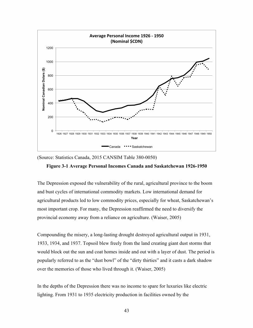
43

(Source: Statistics Canada, 2015 CANSIM Table 380-0050)

Figure 3-1 Average Personal Incomes Canada and Saskatchewan 1926-1950

The Depression exposed the vulnerability of the rural, agricultural province to the boom

and bust cycles of international commodity markets. Low international demand for

agricultural products led to low commodity prices, especially for wheat, Saskatchewan’s

most important crop. For many, the Depression reaffirmed the need to diversify the

provincial economy away from a reliance on agriculture. (Waiser, 2005)

Compounding the misery, a long-lasting drought destroyed agricultural output in 1931,

1933, 1934, and 1937. Topsoil blew freely from the land creating giant dust storms that

would block out the sun and coat homes inside and out with a layer of dust. The period is

popularly referred to as the “dust bowl” of the “dirty thirties” and it casts a dark shadow

over the memories of those who lived through it. (Waiser, 2005)

In the depths of the Depression there was no income to spare for luxuries like electric

lighting. From 1931 to 1935 electricity production in facilities owned by the

0

200

400

600

800

1000

1200

1926 1927 1928 1929 1930 1931 1932 1933 1934 1935 1936 1937 1938 1939 1940 1941 1942 1943 1944 1945 1946 1947 1948 1949 1950

Nom

inal

Can

adia

n D

olar

s ($

)

Year

Average'Personal'Income'1926'4'1950''(Nominal'$CDN)'

Canada Saskatchewan

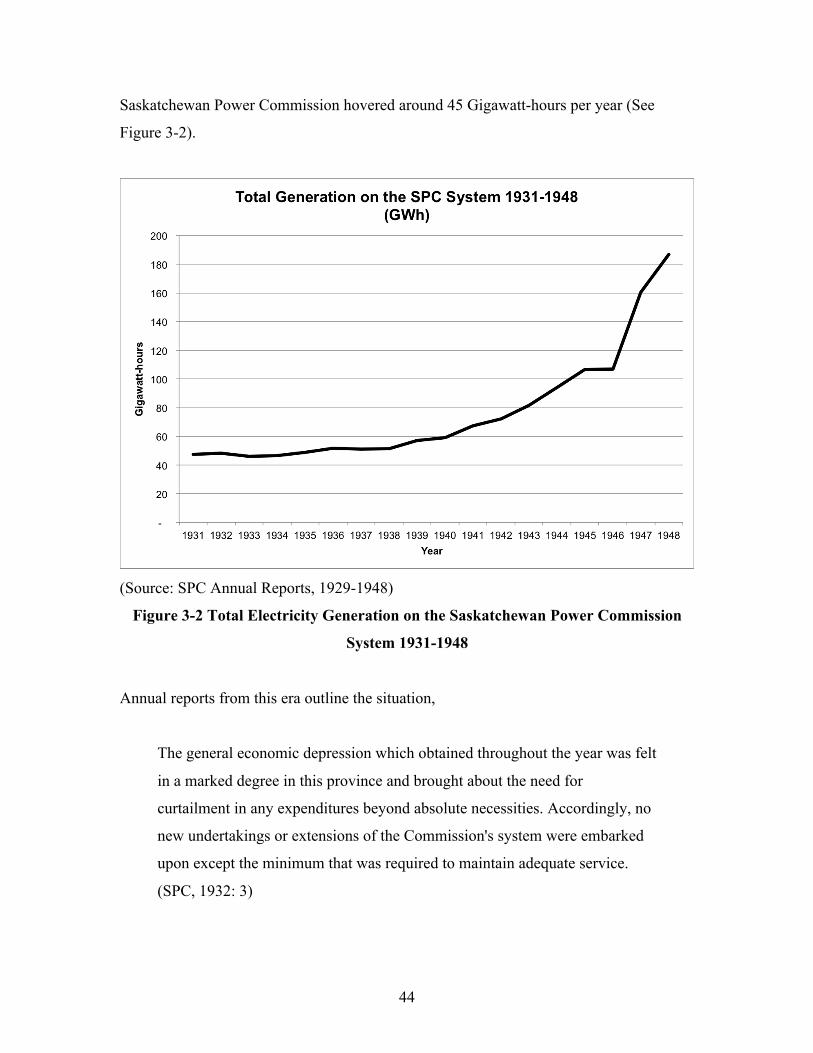
44

Saskatchewan Power Commission hovered around 45 Gigawatt-hours per year (See

Figure 3-2).

(Source: SPC Annual Reports, 1929-1948)

Figure 3-2 Total Electricity Generation on the Saskatchewan Power Commission

System 1931-1948

Annual reports from this era outline the situation,

The general economic depression which obtained throughout the year was felt

in a marked degree in this province and brought about the need for

curtailment in any expenditures beyond absolute necessities. Accordingly, no

new undertakings or extensions of the Commission's system were embarked

upon except the minimum that was required to maintain adequate service.

(SPC, 1932: 3)

45

The general economic depression which obtained throughout the year 1932

has continued during 1933, and, as a result, the demand upon the

Commission's generating plants and transmission line systems has shown no

increase over the preceding year, but is, in fact, very slightly less.

(SPC, 1933: 4)

In this desperate time SPC operated at a loss. Impoverished citizens had a difficult time

paying their bills and SPC employees would accept produce as payment, paying the SPC

the value of the produce, “These were the days when a month’s light account would

purchase a dressed hog or a quarter of beef, often with vegetables thrown in!”

(SaskPower, 1953: 17)

Wartime Scarcity

Power demand began to grow again in step with incomes in the latter half of the 1930s.

For the Saskatchewan Power Commission increasing demand meant increasing revenues

and indicated “a betterment in local conditions in the towns served” (SPC, 1936: 3).

Improving economic conditions in the late 1930s meant that existing infrastructure could

be used at its full capacity. As SPC chairperson Louis Thornton wrote in his 1939 annual

report “Encouraging load increases indicate that more stable economic conditions have

been evident in all districts and bring the total energy demands to proportions which were

contemplated when the systems were built” (SPC, 1939: 4). SPC owned generation

capacity reached 30 MW in 1939 and production increased to 55 Gigawatt-hours in that

year.

Were it not for the intervening conditions of war, the early 1940s might have been a time

of capacity expansion for the Saskatchewan electricity system; demand continued to grow

and investments were badly needed, especially in Saskatoon. Instead wartime restrictions

were placed on the production of non-essential manufactured goods. As Louis Thornton

wrote in the 1941 SPC annual report,

46

It has been evident for some time that additional generation capacity was

urgently required at the Saskatoon plant, and an order for a 15,000 KW turbo-

generator was placed with an English manufacturer in May. Shortly afterward

the British Government issued a suspension order on the construction of this

unit, and, up to the present, efforts made to have the suspension order lifted

and the work put in hand have been of no avail. (SPC, 1941: 3)

This state of rationing continued throughout the war years as materials and labour power

were directed to war-related production rather than domestic goods and services.

Integrating the System

In 1944, the socialist Co-operative Commonwealth Federation (CCF), led by the

charismatic T.C. (Tommy) Douglas, swept into power in Saskatchewan. The CCF

favoured public ownership of industry, and electricity was no exception. Joe Phelps was

appointed Minister responsible for the Saskatchewan Power Commission and soon laid

out a plan to purchase the remaining private and municipal electric utilities companies in

the province and “integrate” the electric system (SPC, 1945). A farmer himself, Phelps

was eager to see the electricity system extend to farms and rural communities. With an

integrated system under public control it would be possible to finance rural electrification

in the province. (White, 1976)

The CCF appointed H.F. Berry to replace Louis Thornton as the commissioner of the

Saskatchewan Power Commission. Berry was a strategic choice as, until his appointment,

he had been the General Manager of the privately owned National Light and Power

Company in Moose Jaw. As such, he could understand the motivations and interests of

the private power producers. (White, 1976)

It is clear that the CCF government wanted Berry to take a more aggressive approach to

fulfilling the mandate of the SPC. The Saskatchewan Reconstruction Council had issued

a report in 1944 criticizing the Commission for its “cautious” approach (p. 148). The SPC

had prevented private companies from expanding electricity service in the province,

47

while also refusing to expand service itself. The province had seen its share of hardship in

the Depression and World War II and so the SPC’s slow progress was not without reason,

but, in the post-war era, progress was expected.

Under instruction from the provincial government Berry began to consolidate the

provincial electricity system. Dominion Electric was first on the list of companies to be

purchased. Dominion generated electricity using lignite coal near Estevan in southwest

Saskatchewan. The purchase would provide SPC with an anchor for the consolidated

system. As the new commissioner for the SPC explained,

The Dominion Electric…Plant at Estevan purchases fuel for one-third the

cost on a B.T.U. basis of cost for fuel at any other location

in…Saskatchewan. The Province, in endeavouring to build up a base power

supply in the Estevan area, will be securing the cheapest source of power in

the Province and, in addition, will be furnishing employment to its own

citizens and using a natural resource of the Province.

(H.F. Berry to Minister Joe Phelps in White, 1976: 140)

Cheap and abundant coal in the southwest of Saskatchewan would be used to generate

electricity that would be transmitted throughout the province and would support the CCF

government’s plans to electrify rural Saskatchewan and promote industrial development.

Coal was also a “natural resource of the Province” and would generate mining jobs in the

Estevan area. Similar arguments in favour of coal reappear in Saskatchewan to this day.

Throughout the late 1940s SPC purchased electricity generation facilities small and large.

In 1945 SPC purchased the Prairie Power Company and folded their operations into SPC

(SPC, 1945). In 1947 SPC purchased Canadian Utilities Limited (SPC, 1947).

As wartime shortages of materials eased, the SPC built transmission lines to connect the

localized electricity distribution networks (White, 1976). Inefficient diesel plants were

closed and expansions were made at centralized generation facilities such as Saskatoon’s

48

coal-fired steam plant. These efforts were directed at creating an “integrated electric

power network” (SPC, 1945: 6).

Integration lowered generation costs and allowed SPC to progressively reduce electricity

rates. In 1945 the maximum rate for electricity sold by the SPC was fifteen cents per

kilowatt-hour (SPC, 1947). Rates were lowered May 1 1945, June 1 1946, July 1 1947,

and June 1 1948 (SPC, 1947; SPC, 1948),

The rate reduction on June 1st, 1948, enabled the Commission to secure

complete uniformity of rate schedules for similar towns throughout the

Province. Street lighting schedules were standardized and rates to rural

customers were reduced along with other rates so that the maximum for any

electrical energy sold by the Commission was lowered to eight cents per

kilowatt-hour. (SPC, 1948: 12)

The rate reductions were aimed at “building load” and they had their desired effect.

Electricity demand began to grow rapidly (See Figure 3-2 above). The Commission also

found itself with a sizable accumulated surplus (See Table 3-2), which would provide

investment capital in the decade to come.

Still, the SPC had not succeeded in creating an integrated system. A report written by

consultant David Cass-Beggs in 1947 was critical of the SPC. Cass-Beggs argued the

SPC had been operating “simply as one of the power companies operating in the province

and serving what loads it could conveniently serve” (Cass-Beggs in White, 1976: 151).

SPC had no success in obtaining the municipal plant at Regina and the privately owned

National Light and Power in Moose Jaw. It had also not made any major progress

towards rural electrification. (White, 1976)

This critique was particularly poignant to the CCF government, amongst whose most

ardent supporters were Saskatchewan farmers. If the SPC could not electrify rural

Saskatchewan it was not doing its job.

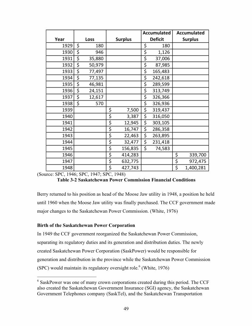
49

(Source: SPC, 1946; SPC, 1947; SPC, 1948)

Table 3-2 Saskatchewan Power Commission Financial Conditions

Berry returned to his position as head of the Moose Jaw utility in 1948, a position he held

until 1960 when the Moose Jaw utility was finally purchased. The CCF government made

major changes to the Saskatchewan Power Commission. (White, 1976)

Birth of the Saskatchewan Power Corporation

In 1949 the CCF government reorganized the Saskatchewan Power Commission,

separating its regulatory duties and its generation and distribution duties. The newly

created Saskatchewan Power Corporation (SaskPower) would be responsible for

generation and distribution in the province while the Saskatchewan Power Commission

(SPC) would maintain its regulatory oversight role.6 (White, 1976)

6 SaskPower was one of many crown corporations created during this period. The CCF also created the Saskatchewan Government Insurance (SGI) agency, the Saskatchewan Government Telephones company (SaskTel), and the Saskatchewan Transportation

Year Loss SurplusAccumulated1

DeficitAccumulated1

Surplus1929 180$'''''''''''''' 180$''''''''''''''1930 946$'''''''''''''' 1,126$'''''''''''1931 35,880$''''''''' 37,006$''''''''1932 50,979$''''''''' 87,985$''''''''1933 77,497$''''''''' 165,483$''''''1934 77,135$''''''''' 242,618$''''''1935 46,981$''''''''' 289,599$''''''1936 24,151$''''''''' 313,749$''''''1937 12,617$''''''''' 326,366$''''''1938 570$'''''''''''''' 326,936$''''''1939 7,500$'''''''''''''' 319,437$''''''1940 3,387$'''''''''''''' 316,050$''''''1941 12,945$'''''''''''' 303,105$''''''1942 16,747$'''''''''''' 286,358$''''''1943 22,463$'''''''''''' 263,895$''''''1944 32,477$'''''''''''' 231,418$''''''1945 156,835$''''''''' 74,583$''''''''1946 414,283$''''''''' 339,700$'''''''''''1947 632,775$''''''''' 972,475$'''''''''''1948 427,743$''''''''' 1,400,281$'''''''

50

SaskPower, the Corporation, “inherited 35 power plants and 4,190 miles of transmission

line” from the Saskatchewan Power Commission (SaskPower, 1969: 25). The task of the

Corporation was to finish the integration that the Commission had begun. This meant

purchasing distribution and generation facilities still held by municipal and private

operators in Regina, Moose Jaw, Weyburn, Swift Current, North Battleford, and Yorkton.

It meant connecting the province with high-voltage distribution lines to allow electricity

to be generated at low-cost sites and distributed through the province. It also meant

extending electrical service to rural Saskatchewan.

Rural Electrification

The CCF government, re-elected in 1948 with the continued support of Saskatchewan

farmers, put a high priority on rural electrification. Joe Phelps, former Minister in charge

of SPC, lost his seat in the 1948 election but stayed on with the SPC board and helped to

develop the Rural Electrification Act, which was signed into law in 1949. This Act

committed SaskPower to build distribution lines to areas where farmers had agreed to

organize and contribute towards the costs. (White, 1976; SaskPower, 1955)

Rural electrification would be an expensive undertaking. There were 125,612 census

farms in Saskatchewan in 1946, and that number fell to 112,018 in 1951 (Ministry of

Agriculture, 2012). These farms were spread throughout the southern part of the province

and the population density of rural areas was low, “The 70,000 farms to be supplied were

scattered in an area of about 130,000 square miles” (SaskPower, 1969: 25). Thousands of

kilometers of distribution lines would have to be built to electrify rural Saskatchewan.

SaskPower began the process of rural electrification by focusing on the rural areas that

were most economical to serve: those along or near existing lines. In 1949, electricity was

connected to 1,142 farms. The next year over 2,000 farms were connected bringing the

total farm and rural customer count to 4,500 (SaskPower, 1950: 5), and in 1951 over

Company (STC), which provides bus service in the province. All of these crowns remain in public ownership today. (Rediger, 2004)

51

3,000 more farms received service. The pace was quickening, but much work remained.

(White, 1976; SaskPower, 1950)

In 1952 The CCF won their third term in office. Tommy Douglas campaigned on a

promise to electrify 40,000 farms and bring electricity to all towns. Charles Smith, rural

electrification superintendent for SaskPower, offered his frank concerns about the

magnitude of this challenge,

This will make a grand total of 56,000 new customers in the next four years!

75% of the total number of customers presently served by the Saskatchewan

Power Corporation (counting the cities of Prince Albert, Yorkton and North

Battleford)! Building in four years many more miles of line than were built in

all the preceding twenty-five years! Providing, as well, extra generating

equipment and main trunk lines to supply these new customers and handle

normal load growth of existing customers! In others words planning, I will

venture to say, a relatively more ambitious program than has ever been

carried out on this continent, or perhaps in the entire world! A program

calling for detailed planning and a ruthless determination to carry it out!

(Charles Smith quoted in White, 1976: 273)

Ruthless determination appears to have been present in the leadership and employees of

SaskPower. SaskPower ramped up rural electrification through the 1950s; over 4,000

farms were connected in 1952 (SaskPower, 1952), 7,500 farms were connected in 1955

(SaskPower, 1955), and 7,800 were connected in the peak year of 1956 (SaskPower,

1969).

Electricity transformed life on the farm, alleviating much of the labour that had

characterized rural life, especially for women (Champ, 2001). Water was pumped, not

hauled to the farmhouse; water heaters replaced the work of boiling water for baths

(Champ, 2001). For those who could afford appliances, electricity soon meant cooking on

an electric range rather than chopping wood to fuel the stove; and washing machines

52

replaced hours of scrubbing clothes on a washboard (Champ, 2001). At least one

awestruck prairie woman (my great-grandmother) was found gazing at her washing

machine as it worked to clean the family linens, watching it as we would a television, still

in disbelief at the labour-saving device.

Rural electrification was a great success and by 1960 the program “was essentially

completed, having brought electricity to about 67,000 farms and to all the villages and

hamlets in the populated half of the province” (SaskPower, 1969: 25). The feat stands as

an impressive demonstration of how the impossible can become possible when motivated

by determined political will and institutional buy-in. It is an example to remember as

SaskPower begins the challenge of electrifying Saskatchewan with sustainable, low

emissions electricity.

Rural electrification was also a great success for the CCF government. CCF leader

Tommy Douglas, the father of Medicare and the first socialist elected to office in North

America, is believed to have said the rural electrification of Saskatchewan was his

greatest achievement (Calvert, 2005). With the goodwill it created for Douglas, rural

electrification may have helped make Medicare possible.

Power for Industry

Farms were not the only new electricity customers in the province in the 1950s.

SaskPower also worked to provide electricity and natural gas sales to Saskatchewan’s

growing industrial sector.7 As SaskPower’s (1957) Annual Report states,

Reaching into more and more of her resource-filled stockrooms – oil, natural

gas, uranium, potash – Saskatchewan has learned that power and natural gas

are the keys to enable these stocks to be taken from storage, processed, and

moved to market. (SaskPower, 1957: 15)

7 “During 1951, the Saskatchewan Power Corporation was designated as the provincial authority to handle the distribution of natural gas” (SaskPower, 1951: 3). It retained this responsibility until 1989 when the SaskEnergy Crown Corporation was created to distribute natural gas (SaskPower, 1989).

53

The oil industry in the province was encouraged to power their pump jacks with

electricity. A salt plant at Unity used substantial electricity and natural gas, both supplied

by SaskPower. Various manufacturing facilities drew from the grid including “a major

cement plant, a clay products plant, and two light aggregate plants at Regina; a fibreboard

plant at Saskatoon; and a clothing plant at Moose Jaw” (SaskPower, 1957: 15).

The potash industry was in its infant stages in the 1950s, but in 1954 SaskPower signed a

five-year agreement with Potash Corporation of America assuring, “if the mining

operations proved successful” the Potash Corporation could count on purchasing “60

million kilowatt-hours” per year from SaskPower by 1958 (Rediger, 2004: 59). The

mining proved more difficult than anticipated, and it was not until 1962 that

Saskatchewan had its first potash mine (Burton, 2014). The potash industry remains one

of SaskPower’s largest customers using electricity for “powering mining machines,

hoisting, conveying, ventilation, lighting, dewatering, mill operations, tailings

management and office/administration facilities” (CIPEC, 2003: 12). The potash industry

drives growth in electricity demand in the present day (Interview 5).8

Beyond the economic development imperative, increased electricity sales to industrial

customers helped to “build load” allowing generation equipment to run during the night

when demand from residential and farms was low (SaskPower, 1952: 10). This in turn

made better use of SaskPower’s generation equipment and helped to further lower

electricity rates. (SaskPower, 1952)

8 It is not clear what rates were charged to each industry, but it was clear that deals were often cut. As the 1952 SaskPower Annual Report revealed, “In co-operation with the Industrial Development Office, special industrial rates were devised to attract industry to Saskatchewan (SaskPower, 1952: 10).”

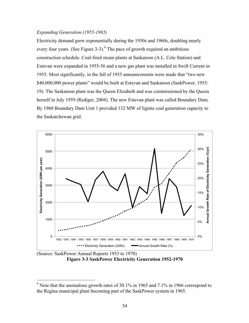
54

Expanding Generation (1955-1965)

Electricity demand grew exponentially during the 1950s and 1960s, doubling nearly

every four years (See Figure 3-3).9 The pace of growth required an ambitious

construction schedule. Coal-fired steam plants at Saskatoon (A.L. Cole Station) and

Estevan were expanded in 1955-56 and a new gas plant was installed in Swift Current in

1955. Most significantly, in the fall of 1955 announcements were made that “two new

$40,000,000 power plants” would be built at Estevan and Saskatoon (SaskPower, 1955:

19). The Saskatoon plant was the Queen Elizabeth and was commissioned by the Queen

herself in July 1959 (Rediger, 2004). The new Estevan plant was called Boundary Dam.

By 1960 Boundary Dam Unit 1 provided 132 MW of lignite coal generation capacity to

the Saskatchewan grid.

(Source: SaskPower Annual Reports 1953 to 1970)

Figure 3-3 SaskPower Electricity Generation 1952-1970

9 Note that the anomalous growth rates of 30.1% in 1965 and 7.1% in 1966 correspond to the Regina municipal plant becoming part of the SaskPower system in 1965.

0%

5%

10%

15%

20%

25%

30%

35%

0

1000

2000

3000

4000

5000

6000

1952 1953 1954 1955 1956 1957 1958 1959 1960 1961 1962 1963 1964 1965 1966 1967 1968 1969 1970

Ann

ual G

row

th R

ate

of E

lect

rici

ty G

ener

atio

n (%

/yr)

Ele

ctri

city

Gen

erat

ion

(GW

h pe

r ye

ar)

Electricity Generation (GWh) Annual Growth Rate (%)

55

SaskPower also made plans to build Saskatchewan’s first hydroelectric plant.

Hydroelectricity had been long studied in the province. In 1927 the Saskatchewan Power

Resources Commission hired consulting engineers Sullivan, Kipp and Chase to study

hydroelectric potential in Saskatchewan. The consultants concluded that a hydroelectric

plant on the Saskatchewan River would not be economical until 1945 when load had

grown substantially (SPRC, 1928; White 1976).

In 1930, after being approached by a proposal from a private developer, the

Saskatchewan Power Commission hired H.G. Acres and Company to study hydroelectric

potential at Fort a la Corne, located just downstream of the junction of the North and

South Saskatchewan Rivers (White, 1976). Acres and Company were optimistic about the

site and believed a hydroelectric project there to be “physically and economically

feasible, and more particularly as a public enterprise” (Acres and Company, 1931: 1).

They estimated that the dam at Fort a la Corne along with transmission to

Saskatchewan’s largest cities “Regina, Moose Jaw, Saskatoon, and Prince Albert” could

be built at a cost of $19,000,000 (White, 1976: 116).

The Depression put the Fort a la Corne proposal on indefinite hiatus. However, H.G.

Acres was asked to update their analysis after World War II. They produced an updated

report in 1946 and recommended the Fort a la Corne project be delayed until electricity

demand had grown; a conclusion similar to that reached by Sullivan, Kipp and Chase in

1928. (White 1976)

With electricity demand growing rapidly in the 1950s SaskPower again looked to

hydroelectricity. The decision was made to build a hydroelectric plant on the

Saskatchewan River near Nipawin at an estimated cost of $46,250,000 or $230 per

kilowatt (in 1959 $CDN dollars) (SaskPower, 1959a). A second hydroelectric station

would be brought into service at Gardiner Dam once that joint federal-provincial project

was complete.10

10 The Gardiner Dam was a $182 million joint federal-provincial project to control streamflow on the South Saskatchewan River and provide irrigation water to farmers.

56

Construction of the E.B. Campbell hydroelectric station began in 1960.11 The project was

producing electricity by 1963, operated at 201 MW in 1964, and was fully commissioned

at 280 MW in 1966. At present it remains in service.

Completing the Integration

The Boundary Dam plant was the fulfillment of the long-sought dream to use cheap and

abundant lignite coal to power the province. With high-voltage transmission lines this

cheap power could be distributed throughout the province and was used as a bargaining

chip to negotiate with the remaining utilities operating outside the SaskPower system.

(White, 1976)

The City of Weyburn agreed to sell its utility in 1957 for “$2,000,000 in annual

installments over a twenty-year period” (White, 1976: 239). When asked how SaskPower

could justify the purchase price General Manager David Cass-Beggs replied that he was

relying “on the availability of cheap Estevan power” (Cass-Beggs quoted in White, 1976:

239). Though Boundary Dam was not yet online, Cass-Beggs had calculated that the low

cost lignite-fuelled power would allow SaskPower to make up the expense through

electricity sales back to Weyburn.

The 64-meter tall Dam created a created a 225-kilometer long reservoir of water that is now called Lake Diefenbaker. At the time of construction it was estimated that approximately 500,000 acres of cropland could be irrigated, increasing the value of output from $7 million to $50 million. As a secondary benefit the dam would also allow for hydroelectric generation; the 187 MW Coteau Creek generating station. The dam was not without impact, however, and valued First Nations cultural artifacts were destroyed, both by the flooding, and intentionally by government officials in order to prevent a hold-up of construction. (CBC, 2015b; Water Security Agency, 2015; Herriot, 2000) 11 The power plant was originally called ‘Squaw Rapids’. In 1987, John Dorion, a native educator, wrote to SaskPower asking them to change the name due to its racist connotations. The head of SaskPower, George Hill, responded by mailing a survey to customers in the same envelope as their power bills asking whether they supported or opposed the name change. Only 1% of SaskPower customers responded, and three-quarters opposed the name change. Hill stood fast. Dorion expressed his disbelief, “It's obvious it’s a racist sign? A survey shouldn't be needed” (Windspeaker, 1987). SaskPower eventually relented and in 1988 the station was re-named to honour former SaskPower President E.B. Campbell.

57

A comparison of costs between local generation and SaskPower rates eventually

convinced the holdout Regina City Council to agree to sell their electric utility to

SaskPower. Regina City Council had remained committed to municipal ownership of the

Regina power plant despite an explosion in 1960 and frequent blackouts in the early

1960s. They had come to enjoy the revenue earned from selling power, as it was a much

less visible source of funds than property taxes. It was not until 1965 that Regina’s

Council faced the realization that rebuilding and retaining their aging power plant would

cost much more than obtaining “cheap Estevan power” from SaskPower. Pressure from

groups such as the Chamber of Commerce likely helped. The Chamber lobbied for the

sale of the Regina power plant, arguing that SaskPower could supply businesses with

electricity at lower rates. (White, 1976)

The sale of the Regina Power Plant and distribution system in 1965 was the final puzzle

piece in creating a truly integrated electricity system in the province. Large coal-fired and

hydroelectric plants provided cheap power and SaskPower distributed the power

throughout the province with a network of high-voltage transmission lines. This publicly

owned system, and the logic of centralized power production, remains in place today.

This 50-year reign has not been without its challenges.

58

The Dawning of Environmental Concern

The E.B. Campbell Dam was SaskPower’s first hydroelectric project.12 More were to

follow. For SaskPower E.B. Campbell was “the first step in a thirty-year plan to harness

electricity from the Saskatchewan River and other northern rivers to meet an increasing

provincial energy demand” (Waldram, 1993: 58). In 1960, General Manager David Cass-

Beggs sketched out a plan for a system of cascading hydroelectric dams along the South

Saskatchewan River (Figure 3-4). Other dams in the remote north would power northern

mining communities.

E.B. Campbell (shown as Squaw Rapids in Figure 3-4) was not without impact. Upstream

from the dam valuable farmland was flooded. Farmers were offered compensation of “2.5

times the assessed value of expropriated land” and further compensation was given for

buildings that had been on the land (Waldram, 1993: 62).

Downstream, the story was different. Cumberland House, a largely Métis community

located downstream from the dam, and the nearby Cumberland House Indian Band,

struggled with the problems created by the dam for years without compensation. On

construction the residents had been assured that the dam would smooth out streamflow on

the river; lowering expected streamflow during summer melt, and increasing streamflow

in winter, when flows were typically low. (Waldram, 1993)

12 The first hydroelectric project was built in Saskatchewan between 1929-1931 and is called Island Falls. This hydro dam is located near the border town of Flin Flon, Manitoba and was built by the Hudson Bay Mining and Smelting Corporation to power their copper and zinc mining operations. SaskPower purchased Island Falls in 1981 and the station, now upgraded to 111 MW of capacity, remains in operation today. (Olsen, 1955; SaskPower, 1981; SaskPower, 2014) Saskatchewan is also home to a partially completed hydroelectric station at Lacolle Falls near Prince Albert. Construction of the $1.2 million dam began in 1912, but a recession, and a lack of access to capital, forced Prince Albert to stop construction in 1913. The City of Prince Albert only finished paying for the expensive and incomplete project in 1965 and the half-completed dam stands as an example of the vulnerability faced by large capital projects. A recent architectural thesis reimagined the incomplete dam as a spa, but as of now it sits in dis-use (Hurd, 2007). (Waiser, 2005)

59

Problematically SaskPower did not plan to operate the dam in this manner. E.B.

Campbell, Assistant Chief Engineer of SaskPower, whose name would eventually adorn

the dam, stated internally, “The Squaw Rapids project will be operating as a peaking

plant, at least during heavy load season, and this will result in extremely large daily

fluctuations in discharge” (Campbell quoted in Waldram, 1993: 63).

The results were decidedly negative for Cumberland House. Residents in the area relied

on fishing, trapping, and tourism for their livelihoods. In a letter to the Provincial

government in 1964, the President of the Cumberland House Fisherman’s Cooperative

described the impact,

From the time the Squaw Rapids dam has been operational, we have noted

the following:

Fish have been caught in deeper holes in rivers and lakes, when the

water flow is suddenly reduced. Fishing operations carried on elsewhere have

had to be abandoned. If the situation is reversed, the fish drown on sudden

high levels. We suffer heavy losses both ways.

Sudden high water destroys nests of waterfowl during nesting seasons.

Income usually derived from this source of guiding and hunting by natives is

lowered.

At this time of writing, the species of wildlife suffering most from the

consequences are big game. Their young are being caught in lowlands and

drowned in the rise of water. The latter effects on fur bearing animals will

also be greatly felt. The unsteady flow is definitely hampering with

conservation.

We trust that our plea will reach sympathetic ears. We are a people

depending on these sources for a living. We ask for more consideration from

the management of the dam and your support before our plight is increased.

(Waldram, 1993: 68)

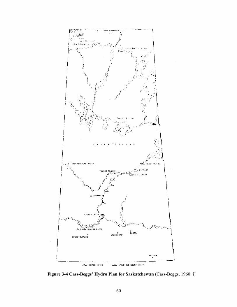
60

Figure 3-4 Cass-Beggs’ Hydro Plan for Saskatchewan (Cass-Beggs, 1960: i)

61

The pleas of the community did not reach sympathetic ears. E.B. Campbell, in the same

SaskPower internal memo quoted above wrote,

I don’t think that we can be expected to limit operations at the Squaw Rapids

site to protect beaver and muskrats…Any restriction on (dam operation) in

the interests of wildlife will, no doubt, result in economic losses to the hydro

project that will greatly exceed the value of any fur bearing animals.

(Waldram, 1993: 63)

Though SaskPower believed its hydro-power had a higher market value than the

fur-bearing animals downstream, the corporation did not compensate fishers or

trappers for the external costs imposed by the dam. The only downstream entity to

receive compensation from SaskPower was an outfitting company called Les

Voyageurs, who were paid $1500 in 1963 because the dam had reduced fall

streamflow and shortened their outfitting season. In exchange, Les Voyageurs

agreed they would not file a lawsuit against SaskPower. (Waldram, 1993)

Rather than offering compensation, SaskPower and the Saskatchewan government

reacted to the letter from the President of the Fisherman’s Co-operative by studying the

downstream impacts of the dam. Mitigation was deemed too expensive. The community

continued to press the government for compensation. More studies were commissioned.

After years of delay the community grew frustrated by the government’s “more study –

no action” approach and launched a legal challenge for compensation (Waldram, 1993:

74). The government in turn offered to continue negotiations. In good faith the

community put the lawsuit on hold. A mediator was appointed in 1986, but progress was

slow. In 1987, to press home their demands, hundreds of community members even

began constructing their own dam to “raise the level of Cumberland Lake” and improve

downstream conditions (Waldram, 1987: 78). Waldram writes, “Ironically, the

Saskatchewan government’s Department of the Environment expressed concern that not

only was the dam illegal, but also that it could cause environmental damage” (1987: 79).

62

In 1989, over twenty-five years after the dam was constructed, a compensation package

was awarded to the community worth an estimated $25 million dollars. (McLennan,

2008)

During the struggle with SaskPower, other dams were proposed. A dam at Nipawin was

proposed in the mid 1970s and was built upstream from E.B. Campbell in the 1980s. A

dam was also proposed for the Churchill River at Wintego Rapids. The proposition was

contentious. The Churchill River was a prized destination for recreational canoeing and

fishing, and is home to a rich aquatic ecosystem. The government organized the Churchill

River Board of Inquiry to seek public input on the Wintego dam proposal. The residents

of Cumberland House made sure to let the commission, and those living downstream

from the dam, know what to expect; a damaged ecosystem and a Corporation unwilling to

compensate for the damage. The final report of the Churchill River Board of Inquiry was

released in 1978 and summarized public opposition to the Wintego project. The dam was

scrapped. (Waldram, 1994; SaskPower, 1991a; Rediger, 2004)

SaskPower’s plans to expand coal-fired generation were also generating local

environmental concern. In 1975 SaskPower expressed interest in building another coal-

fired plant near Coronach. Farmers in the area were concerned that local coal-mining

would damage valuable farmland. Many had been to Estevan and had seen firsthand the

“moonscape” that had been created by surface mining coal (Rousseau, 2014). Coronach

area farmers formed a surface rights group and lobbied to have the mining companies

store the topsoil when they removed it, and replace the ‘overburden’ and topsoil when

they were finished. This practice would ensure that agriculture could continue in the area

after the coal had been mined. (Rousseau, 2014)

The remediation practices have been a success. Around the Poplar River plant hay fields

now cover what used to be coalmines. For residents of Coronach the environmental

remediation, won through the advocacy of local farmers, is a source of pride (Rousseau,

2014). SaskPower learned a valuable lesson in the importance of obtaining social license

for their projects.

63

Still, concern over local environmental impacts of planned power projects continued to

plague SaskPower into the 1980s. North of Coronach, a planned coal-fired plant near was

“blocked in 1981 when the Rural Municipality Gravelbourg designated four heritage sites

in the area” (Rediger, 2004: 123). To supply their coal-fired power plant with cooling

water SaskPower had planned to dam the Wood River and create a reservoir. If the dam

were built, three of the newly designated heritage sites would be flooded. SaskPower

disputed the size of the heritage sites and wanted to see them reduced. A third-party

investigation was carried out, which concluded, “Staggering quantities of heritage

resource information exists in the proposed Cooper reservoir. Reservoir construction and

inundation will probably completely destroy the information potential of all heritage

resources occurring in or near the impact zone” (LeaderPost article quoted in Rediger,

2004: 123). The reservoir and the power plant did not proceed.

The most notorious power siting conflict in Saskatchewan occurred when SaskPower

made plans to supply cooling water for the proposed Shand coal-fired power plant near

Estevan. Two dams were planned: the Rafferty and the Alameda. These dams would offer

cooling water for Shand, and would control streamflow on the Moose Mountain creek

and the Souris River. Project proponents argued the flow control would protect the city of

Minot in North Dakota from flooding. (Jowett, 2012)

When two farmers, Ed and Harold Tetzlaff found out the Alameda dam would flood their

land they took action to stop it. With other affected landowners the two brothers started

an organization called SCRAP ‘Stop Construction on Rafferty-Alameda Projects’. The

farmers were joined by the Saskatchewan Wildlife Federation, an organization that grew

concerned that the projects would destroy valuable wetlands. (Jowett, 2012)

Trouble arose when the Federal Minister of the Environment, Tom McMillan issued an

approval of the Rafferty-Alameda project without the project having gone through an

64

environmental assessment. One of McMillan’s senior aides resigned over the decision.

Her name was Elizabeth May.13 (Jowett, 2012; Harrison, 1996)

May caused an uproar when she went public with the reason for her resignation. May

alleged that the decision to approve Rafferty-Alameda without an environmental review

was the result of a political deal cut between the Federal Government and the

Government of Saskatchewan. Critics of the decision believed it went against the Federal

government’s own Environmental Assessment and Review Process (EARP) Guidelines,

published in 1985 (Environment Canada, 1985). The Canadian Wildlife Federation took

the federal government to court demanding an environmental assessment be completed.

(Jowett, 2012; Harrison, 1996)

Rafferty-Alameda was a landmark case in environmental law. The federal court decided

for the plaintiff and against the Federal government. They ruled that the EARP

Guidelines were binding and that the Federal government had an obligation to conduct an

environmental assessment on the project. (Harrison, 1996)

The courts did not, however, approve an injunction to halt construction of the project.

Construction continued, the dams were completed in 1991, and Ed and Harold Tetzlaff

lost their farmland. The brothers had, however, won a victory for environmental groups

in Canada,

Although only thirty-five proposals were referred for public reviews by the

federal government in the fifteen-year period from 1974 to 1989, there were

twenty-four reviews in less than two years after the Rafferty-Alameda

decision. (Harrison, 1996: 134)

SaskPower worked to respond to the rise of environmental concern. In 1972 SaskPower

CEO warned presciently of the challenges to come,

13 May now leads the federal Green Party.

65

The development of energy resources to meet the anticipated growth in

demand for power and gas services in the face of rising costs and increased

public concern on environmental matters is the most important challenge

facing the Corporation in the future. While on one hand the Corporation is

committed to the development of energy resources to meet the growing

demands of its customers, it also stands committed to the orderly and

economic development of these resources, and to minimizing the undesirable

environmental impact of such activities. (R.R. Keith in SaskPower 1972: 3)

In 1980, SaskPower conducted an internal reorganization that created several new

business units in “energy supply planning, environmental protection, energy conservation

and public participation” (Rediger, 2004: 121). The CEO at the time, Robert Muncor,

described the need to balance costs, environmental, and social concerns,

The very major challenge is to provide the (power) needs of the province in

a reasonable way, reasonable meaning at as low a cost as possible, in as an

environmentally and socially sound way as those objectives can be balanced

together. (Muncor quoted in Rediger, 2004: 123).

In 1989 George Hill, then CEO of SaskPower wrote of the corporation’s progress and

aspirations,

In 1989, SaskPower formalized a comprehensive Environmental Policy

Statement, which confirms that environmental responsibility has always been

a priority. It provides a framework in which we can protect the environment

while continuing to meet the province’s electrical needs. We intend to make

SaskPower the most environmentally responsible power utility in Canada.

(George D. Hill in SaskPower, 1989: 6)

66

By the early 1990s it was clear that a sea change had occurred in public perception of

power production. The public had realized that electricity generation, of any type, has an

environmental and social impact.

What was once thought of as an environmentally benign source of energy has

been linked to ozone depletion, acid rain, the greenhouse effect and other

negative environmental concerns such as flooding, water diversion and

radioactive contamination. (SEEORP, 1991: 3)

In 1992, the coal-fired Shand Power station was commissioned. The Rafferty-Alameda

dams that provided reliable cooling water for the plant had flooded valued farmland and

wetlands, but SaskPower claimed that Shand would be an environmentally sustainable

power plant. Shand’s cooling water would heat a greenhouse where native tree saplings

would be grown, and these would be distributed around the province. As a further benefit

the trees would act as carbon sinks. Shand was also equipped with a limestone scrubber

system to minimize sulphur dioxide emissions and lessen the plant’s contribution to acid

rain. (SaskPower, 1993)

In 1993, Shand, the power plant, whose cooling reservoirs had been built without

environmental assessment and set a ground-breaking precedent in environmental law,

was honoured “with the prestigious Power Plant Award” for its sulphur dioxide control

systems and “zero discharge water management system” (SaskPower, 1993: 6). Without a

hint of irony SaskPower called Shand “Canada’s most environmentally friendly coal-

fired station” (SaskPower, 1993: 6).

Beyond the Public Power Coal-Hydro Nexus

As outlined above, Saskatchewan’s publicly owned power system was built to transmit

electricity from southeastern coalfields and hydroelectric plants along the Saskatchewan

67

River system.14 These centralized plants replaced more expensive distributed diesel

turbines, and public ownership allowed SaskPower to charge lower prices for electricity

than private utilities.

The logic and the design of the system did not change in a quarter of a century. In 1992,

coal made up 71% of electricity generation, hydroelectricity provided just over 20% of

electricity, natural gas provided 4.5%, with imports of hydroelectricity from Manitoba

providing the remaining power (SaskPower, 1992).

The system also remained in public ownership. In 1991 the Saskatchewan Electrical

Energy Options Panel (SEEOP) observed, “all the electrical energy supplied to the grid

connected Saskatchewan system comes from generating facilities owned and operated by

SaskPower or from neighbouring utilities” (SEEOP, 1991: 18). SaskPower had survived

under public ownership despite two previous periods when the ruling political parties

prioritized privatization and free enterprise.

The first wave of privatization in Saskatchewan came during the period of 1964-1971

under Liberal Premier Ross Thatcher. Thatcher was a former member of the CCF, but in

the 1964 election he campaigned as Liberal leader on a platform emphasizing lower taxes

and less government control of business. Thatcher and the Liberals won the election,

unseating the CCF and ending their 20-year reign. (Rediger, 2004)

During the election campaign Thatcher spoke of his desire to sell off struggling crown

companies. Crowns would be sold unless they met one of three criteria, providing “an

essential service which private firms are unable to supply at a comparable cost to the

public”, providing “useful employment which otherwise would not be available” or

offering “a particularly satisfactory return on invested public funds” (Thatcher quoted in

14 At least the southern portion of the system. The northern system is predominantly hydroelectric and diesel and was built in a piecemeal fashion to coincide with mining developments and isolated settlements.

68

Rediger, 2004: 76).15 SaskPower was a profitable crown in most years and provided

dividends to the provincial government, meeting the third criteria. With the memory of

the cross-subsidized rural electrification campaign fresh in the minds of Saskatchewan

residents, SaskPower also likely passed the first test and provided a service that a private

operator would not have supplied. This meant that, despite the ideology of the Thatcher

Liberals, SaskPower was safe from privatization during their time in power.16 (Rediger,

2004)

Thatcher’s Liberals lost to the New Democratic Party (NDP) – a reinvented CCF – led by

Allan Blakeney in the 1971 election. Thatcher died three months later (Rediger, 2004).

Blakeney brought a renewed commitment to public ownership, and expanded

Saskatchewan’s portfolio of Crown corporations. Of particular note, Blakeney formed the

Potash Corporation of Saskatchewan (PCS) as a vehicle to purchase (or expropriate if

need be) potash ventures in the province (Burton, 2014).

A second wave of privatization occurred during 1982 – 1991 under Premier Grant Devine

and the Progressive Conservative (P.C.) government. The P.C.’s welcomed “public

participation” in the economic life of Saskatchewan. The Orwellian phrase referred to

Saskatchewan citizens holding stocks in privately owned Saskatchewan corporations.

(Rediger, 2004)

The Potash Corporation of Saskatchewan, newly formed in 1975, was sold off by the

P.C.s in 1989-1990 (Burton, 2014). It is now one of the world’s largest potash mining and

15 Thatcher’s tenure was marked by poor labour relations at SaskPower. In 1966 workers on the natural gas side of the company went on strike to demand an 8% pay increase. The Liberals brought the strike to an end by passing essential services legislation in the form of the Essential Services Emergency Act. The Act allowed government to declare a state of emergency and implement compulsory arbitration when a strike threatened “life, health or property” (Rediger, 2004: 87). A strike by natural gas workers was deemed to fit that criterion. A strike by the electrical workers was narrowly averted at the bargaining table in 1969 (Rediger, 2004). 16 Of note, Ross Thatcher’s son Colin became an MLA like his father. Colin Thatcher resigned his post as Minister of Energy and Mines in 1984 when he was convicted of killing his wife JoAnn Wilson.

69

integrated fertilizer companies, and earned over $7 Billion in revenue in 2014

(NASDAQ, 2015; Burton, 2014). The Saskatchewan Mining and Development

Corporation (SMDC), a provincial crown formed to mine uranium in northern

Saskatchewan, was combined with Eldorado (a federal uranium mining crown) in 1988.

Shares were opened for “public participation” in 1991. CAMECO is now the largest

uranium mining company in the world.

The P.C.s planned to privatize the natural gas distribution functions of SaskPower.

Taking a step down this path, SaskPower was split in two in 1989: SaskEnergy would

handle natural gas sales and distribution; SaskPower would continue to control electricity

supply in the province (SaskPower, 1989). When the split was finalized George Hill,

head of SaskPower, remarked,

(SaskEnergy) is the only gas distribution company that is now owned by

government. Every other gas distribution company (in Canada) is investor-

owned…I firmly believe that every person in Saskatchewan should have an

opportunity to participate.

(George Hill quoted in Rediger, 2004: 152).

In April 1989 the P.C.s announced plans to privatize the newly created SaskEnergy. The

profits would be used to pay down SaskPower’s debt, which had grown to $2 billion by

1988 (Rediger, 2004; SaskPower, 1988). The debt was in part due to high financing

charges. Interest rates had spiked in the early 1980s and remained at historically high

levels throughout the decade increasing the cost of capital for SaskPower (See Figure 3-

5).17

When plans to sell SaskEnergy were announced, the NDP staged a 17-day walk out from

the legislature. It was not until the P.C. government promised a commission to study the

impacts of privatizing SaskEnergy that the NDP returned. The commission reported in

17 In 1986 SaskPower’s revenue was $507 million (1987 CDN dollars) and financing charges were $214 million, a full 40% of revenue. (SaskPower, 1993)

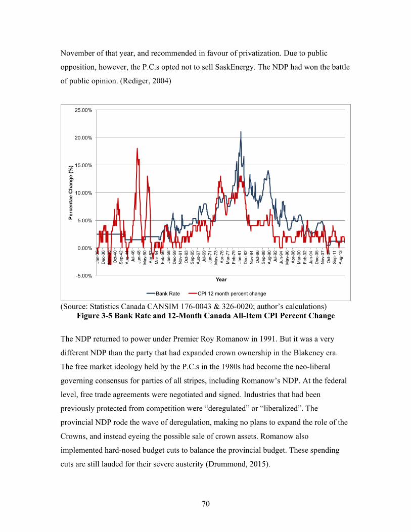
70

November of that year, and recommended in favour of privatization. Due to public

opposition, however, the P.C.s opted not to sell SaskEnergy. The NDP had won the battle

of public opinion. (Rediger, 2004)

(Source: Statistics Canada CANSIM 176-0043 & 326-0020; author’s calculations)

Figure 3-5 Bank Rate and 12-Month Canada All-Item CPI Percent Change

The NDP returned to power under Premier Roy Romanow in 1991. But it was a very

different NDP than the party that had expanded crown ownership in the Blakeney era.

The free market ideology held by the P.C.s in the 1980s had become the neo-liberal

governing consensus for parties of all stripes, including Romanow’s NDP. At the federal

level, free trade agreements were negotiated and signed. Industries that had been

previously protected from competition were “deregulated” or “liberalized”. The

provincial NDP rode the wave of deregulation, making no plans to expand the role of the

Crowns, and instead eyeing the possible sale of crown assets. Romanow also

implemented hard-nosed budget cuts to balance the provincial budget. These spending

cuts are still lauded for their severe austerity (Drummond, 2015).

-5.00%

0.00%

5.00%

10.00%

15.00%

20.00%

25.00%

Jan-

35

Dec

-36

Nov

-38

Oct

-40

Sep

-42

Aug

-44

Jul-4

6 Ju

n-48

M

ay-5

0 A

pr-5

2 M

ar-5

4 Fe

b-56

Ja

n-58

D

ec-5

9 N

ov-6

1 O

ct-6

3 S

ep-6

5 A

ug-6

7 Ju

l-69

Jun-

71

May

-73

Apr

-75

Mar

-77

Feb-

79

Jan-

81

Dec

-82

Nov

-84

Oct

-86

Sep

-88

Aug

-90

Jul-9

2 Ju

n-94

M

ay-9

6 A

pr-9

8 M

ar-0

0 Fe

b-02

Ja

n-04

D

ec-0

5 N

ov-0

7 O

ct-0

9 S

ep-1

1 A

ug-1

3

Perc

enta

e C

hang

e (%

)

Year

Bank Rate CPI 12 month percent change

71

In this era of deregulation and neo-liberalism SaskPower’s CEO Jack Messer, newly

appointed by the NDP when they returned to power, believed it was important that

SaskPower adapt to the realities of a deregulated electricity market. Messer believed that

SaskPower should prepare for competition,

The business landscape in which SaskPower operates is undergoing dramatic

change. Deregulation of the electric industry in the United States has opened the

doors to competition, setting the stage for similar circumstances in Canada. The

American example is showing us the impact of a shifting market for electrical

energy, transforming a once-stable, secure business environment into one facing

the uncertainties of open competition for power generation, transmission and

distribution. Within this new competitive environment, price and service

become the keys to sustaining existing business and attracting new customers.

(Jack Messer in SaskPower, 1994: 4)

Preparing for competition meant drafting policy that would allow other power generators

access to the Saskatchewan grid (SEEOP, 1991). Messer worked to prepare SaskPower

for this competition, but was fired from his position in 1997 before the job was

complete.18

Messer was succeeded by John Wright, a former Deputy Minister of Finance for the

provincial government. Under Wright’s leadership the Saskatchewan grid began to move

away from the publicly owned coal-hydro nexus. Wright was willing to explore private-

public partnerships in the form of “cogeneration.” He also explored ways to move away

18 Messer’s firing was related to the sale of a SaskPower venture called Channel Lake Petroleum Ltd. Channel Lake was created in 1993 as a SaskPower subsidiary. Its role was to purchase natural gas for SaskPower. The venture fared poorly and by 1997 had lost $8 million. SaskPower negotiated the sale of Channel Lake to Alberta based Direct Energy Marketing Ltd for $20.8 million. When it came time to sign the contract, however, the SaskPower team didn’t notice that the fine print that subtracted $5.2 million from the price they thought there were getting. Signed contract in hand the purchasing party bought Channel Lake at a steep discount. Messer was fired for the error. The general manager of Channel Lake, who had negotiated the sale, was also fired and went on to work for Direct Energy. (Rediger, 2004)

72

from SaskPower’s reliance on coal. The Kyoto protocol had raised the possibility of

greenhouse gas emissions regulation. Despite regulatory uncertainty from the federal

government, SaskPower began creating annual climate change “action plans” to take “a

proactive approach to reducing and mitigating greenhouse gases” (SaskPower, 2001: 10).

Natural gas power generation was an appealing option for SaskPower since it emitted

greenhouse gas emissions roughly one-third that of coal per unit of electricity generated.

(Wright, 2014)

The first cogeneration project was a natural gas combined cycle unit at Lloydminster.

Owned by TransAlta cogeneration, the facility supplies steam to Husky’s Lloydminster

heavy oil upgrader and sells electricity to SaskPower on a long-term purchase agreement.

The Meridian project was commissioned in 2000. (SaskPower, 2001; Wright, 2014)

The next cogeneration was created through a private-public partnership agreement with

ATCO, a private utility based in Alberta. ATCO and SaskPower partnered to build a

cogeneration plant at the Cory potash mine owned by the Potash Corporation of

Saskatchewan (the former crown now operating as a private company). The 228 MW

combined cycle natural gas facility provides steam for potash mining process operations

and electricity for the Saskatchewan grid. The Cory cogeneration plant was

commissioned in 2003. (SaskPower, 2001-2003; Wright, 2014)

The move to cogeneration was not full-blown privatization, but was a shift from

SaskPower’s former policy of exclusively building, owning and operating generation

facilities. The phrase “co-generation” referred both to the technology being employed and

generation owned in partnership with another private entity. The move to open new

generation projects up to public tender won approval from groups such as the libertarian

minded Frontier Centre for Public Policy (1999) who celebrated the Meridian

cogeneration project as a successful step in the right direction, “It's taken a couple of

generations, but marketplace realities are displacing the old ideas of state control and

ownership.” Under John Wright and the Romanow NDP, the public power system had

begun to open to private ownership. The introduction of natural gas also reflected a shift

73

away from the coal-hydro nexus that had powered the province for the previous forty

years.

The Arrival of Wind Power

Wright’s desire to lower GHGs and diversify the SaskPower electricity system led him to

approve the first utility-scale wind turbine project in Saskatchewan. The SunBridge Wind

Power Project was a privately owned joint venture between Suncor Energy Inc. and

Enbridge Inc., familiar names in the oil and gas industry. The 11 MW project was built in

2002 in southwest Saskatchewan (SaskPower, 2001: 8). SaskPower built its own 5.9 MW

facility in the same region, beginning full operation the following year. (SaskPower,

2001; SaskPower, 2002; SaskPower, 2003; Wright, 2014)

Wind had been under consideration in different forms for many years. There is a

reference to farmer-owned “wind machines” in the Saskatchewan Reconstruction Council

report of 1944. At that time, wind turbines, partnered with batteries, offered the

possibility of supplying power to farmers located far from the existing grid. Several

farmers did install these systems to power yard lights and water pumps. (Saskatchewan

Reconstruction Council, 1944)

In 1974 SaskPower tested an “experimental model of a small wind turbine developed by

the National Research Council” to see how it would fare under “Saskatchewan

conditions” (SaskPower, 1974: 10).

SaskPower also explored building a commercial-scale wind project in the 1990s, but the

project was rejected by Jack Messer who stated,

In the final analysis, it was decided the cost premium associated with

proceeding with the project could not be justified. In today’s rapidly changing

business environment, it is critical to SaskPower’s customers that efficiencies

are achieved wherever possible.

(Jack Messer in Government of Saskatchewan press release, 1995)

74

The wind projects in the early 2000s were small and exploratory, but offered substantial

returns. Southwest Saskatchewan is home to a rich wind resource and the turbines

regularly achieve capacity factors of 40% (Interview 2). Their success, and pressure from

environmentally minded members of the provincial NDP such as Peter Prebble, led

SaskPower to build a larger project in 2005; the 150 MW Centennial wind power facility.

(Wright, 2014)

At present SaskPower continues to expand wind power, albeit in a slow and cautious

manner. The preferred approach is to issue a call for proposals for wind power projects

and allow private wind developers to respond. This puts developers in the position of

identifying wind resources, securing land lease agreements, and seeking community

support. SaskPower then agrees to purchase power from one or more of the applicants.

Two recent wind projects; at Chaplin and Moosomin respectively were approved in this

manner. (Confidential interviews, 2015)

The potential for wind substantially outstrips the installed capacity. SaskPower recently

issued a call for proposals seeking 200 MW of new wind capacity. The market returned

4000 MW of interest (Confidential interviews, 2015). Despite this rich resource, wind

made up only 2.7% of electricity generated in Saskatchewan in 2014 (SaskPower, 2014).

Advocates of wind energy have been increasingly vocal in asking SaskPower to speed up

investment in wind power. Saskatchewan Community Wind, set-up by James Glennie,

has been working to build support for a community-owned wind project in the Saskatoon

area. The Green Energy Project of Saskatchewan (GEPS) has outlined pathways to

increase wind and solar in the province (Bigland-Prichard & Prebble, 2010; Bigland-

Prichard 2010; Bigland-Prichard 2010a; Bigland-Prichard 2011). These advocates call for

SaskPower to move from 2.7% wind to 25% wind power on the grid in short order.

Problematically SaskPower values wind only as a means of reducing their natural gas

expenses. Wind’s electricity output is variable, and SaskPower must back-up wind

capacity with fast-ramping natural gas single-cycle or combined-cycle turbines. The

75

value of power generated by wind power is thus discounted and is valued at the cost of

avoided natural gas consumption – about 3.5-4 cents/kilowatt-hour – rather than the

wholesale electricity rate. (Interview 6)

Even as a means of reducing natural gas consumption wind is likely to be more important

in the future. We live in an era of low natural gas prices, but this was not always so. The

oil crisis of 1979 led to spikes in the price of oil and natural gas. Natural gas prices were

also high in the early 2000s. Soon after expanding natural gas capacity with the

Lloydminster Meridian cogeneration project SaskPower found itself stung by rising

natural gas prices (SaskPower, 2001). A drought in 2001 led to lower than usual

hydroelectric production and further worsened the crisis (SaskPower, 2001). As John

Wright says of the period, “we were getting hammered by natural gas prices, just

creamed!” (Wright, 2014). The volatile price of natural gas remains a challenge for

SaskPower’s planning at present.

Wind may be the preferred source of power generation by civil society actors such as the

Green Energy Project of Saskatchewan (GEPS), but not all Saskatchewan citizens are

thrilled with the technology. Residents of the Rural Municipality (R.M.) of South

Qu’Appelle, located 20 kilometres east of Regina, said no to a proposed 50 MW 50-

turbine wind project in March 2014. Renewable Energy Systems Canada (RES) had

hoped to install a wind monitoring station in the R.M. After significant public outcry, the

R.M. passed a motion outlining that wind monitoring stations and wind farms would not

be allowed (Shepherd, 2014). This despite the fact that the region allows high-impact

uses such as intensive-livestock operations.

The renewables are not getting any political support from the governing Saskatchewan

Party. Instead Premier Brad Wall has retained a dogged fascination with nuclear power.

Recent statements on CBC indicate that the Premier hopes for federal government

support for replacing coal-fired generation with nuclear power (CBC, 2015a).

76

The Nuclear Dream

The Saskatchewan Party was elected in 2007, ending the sixteen-year tenure of the NDP

under Roy Romanow and, after 2001, Lorne Calvert. One of Saskatchewan Premier Brad

Wall’s first actions was to set up the Uranium Development Partnership (UDP) to study

the future of uranium in Saskatchewan. The UDP was an industry-stacked panel of

twelve that included the CEOs of uranium mining companies CAMECO (Jerry Grandey)

and AREVA Canada (Armand Lefèrrere), and the CEO of nuclear power producer Bruce

Power (Duncan Hawthorne). The board also included an environmental representative,

the infamous Patrick Moore, who has made a living advertising his former ties to

Greenpeace while advocating for industries such as nuclear power and chemical

pesticides. (UDP, 2009)

It came as no surprise that the UDP recommended: the expansion of the uranium mining

industry in Saskatchewan; the building of a nuclear power plant; construction of a

research reactor to create medical isotopes; and storage of nuclear waste in the province

(UDP, 2009).

To their credit the Government of Saskatchewan took these recommendations to the

people of Saskatchewan. Long-time civil servant Dan Perrins was asked to visit

communities across the province to get citizen feedback on the recommendations.

Hundreds of citizens attended the public meetings and nearly all of them opposed the

proposed expansions of the uranium industry (Perrins, 2009).19

Opposition to a nuclear power plant was particularly strong in the Lloydminster area. In

2008, Bruce Power, eager to capitalize on the provincial government’s support for

nuclear power, conducted a feasibility study into building a 1000 Megawatt (MW) reactor

in Saskatchewan (Bruce Power, 2008). They selected Lloydminster as a candidate site for

19 In statistical terms, 84% of submissions (oral or written) that touched upon nuclear power opposed nuclear power; on the issue of nuclear waste storage in the province 86% of submissions that addressed that issue were opposed.

77

the plant. Straddling the Alberta-Saskatchewan border, Lloydminster would allow the

possibility of electricity exports to the Alberta grid (Bruce Power, 2008).

In early 2009, before the UDP consultations had occurred, Bruce Power began

approaching ranchers in the Lloydminster area to secure a location for a nuclear power

plant. One ranching family had just celebrated the centennial anniversary of their family

operation, only to find out that Bruce Power was planning to purchase land next door.

Concerned about the impact to their land and their children’s health, the ranchers

organized a group called ‘Save Our Saskatchewan’ or S.O.S. for short. S.O.S. and other

groups in the province attended the public meetings, wrote letters to their MLAs, and sent

a message to Premier Wall that nuclear power was not wanted in Lloydminster, or

anywhere in the province.

The Government of Saskatchewan responded to public opposition by stating that they had

received a “yellow light” for moving ahead on the UDP recommendations (White, 2009).

This yellow light soon turned green for uranium mining expansions, nuclear waste

storage proposals, and a nuclear-uranium research centre at the University of

Saskatchewan. The green light also appears to be back on for nuclear power. Premier

Brad Wall has recently indicated his support for building small-modular nuclear reactors

in the province (CBC, 2015a).

While the Saskatchewan Party government has been a public advocate of nuclear power

in the province, SaskPower has looked at the possibility for several decades. As early as

1955 SaskPower was sending staff for “training in atomic energy plant design”

(SaskPower, 1955: 27). SaskPower also drew a link between uranium mining in

Saskatchewan’s north and the future of nuclear power in the province,

In Saskatchewan’s north, electrical power assists mining companies in the

Beaverlodge area to recover another vital source of power – uranium – which

will some day soon, in its turn, be added to the fuels used to generate still

more electrical power. (SaskPower 1957: 15)

78

In 1973, SaskPower CEO R.R. Keith wrote, “Nuclear energy is expected to play a

significant role in the Provincial energy supply in the long term as it will probably be

competitive before Saskatchewan’s coal resources are fully developed” (SaskPower,

1973: 2). There was the sentiment at that time that nuclear power would become “too

cheap to meter” and was the electricity generating option of the future.

Under R.R. Keith’s leadership SaskPower took a close look at nuclear power in the early

1970s. In preparation for a possible investment SaskPower commissioned a series of

reports: a review of nuclear technology in 1972, a Feasibility Study for a Nuclear Power

Program in 1973, and an analysis of potential sites for a nuclear power plant in 1975

(SaskPower, 1972a; SaskPower, 1973a; SaskPower, 1975a). A chief concern in the 1975

report was the availability of cooling water on the arid prairies. Possible nuclear power

sites were centered on reliable water supplies like the South Saskatchewan River, Last

Mountain Lake, and Lake Diefenbaker; the lake that had been created with the

construction of the Gardiner Dam in the 1960s (SaskPower, 1975a).

The 1970s, however, turned out to be a bad time to invest in a nuclear mega-project, not

only for Saskatchewan, but for utilities across North America. During this “difficult

period” costs were spiraling upwards for electrical utilities (Ford, 1997). Inflation rates

were high, which increased the cost of building nuclear plants. High interest rates made

borrowing to finance capital construction more expensive (see Figure 3-5 above). New

plants also took longer to build, and the delay between construction and production

increased costs. (Ford, 1997)

Utilities that signed on for large capital projects like nuclear power plants were forced to

increase electricity rates, but this had the effect of curbing the growth of electricity

demand and reducing revenues. Fears abounded that utilities had entered a “death spiral”

(see Figure 3-6) of increasing costs and decreasing demand that could bankrupt the

industry. (Ford, 1997)

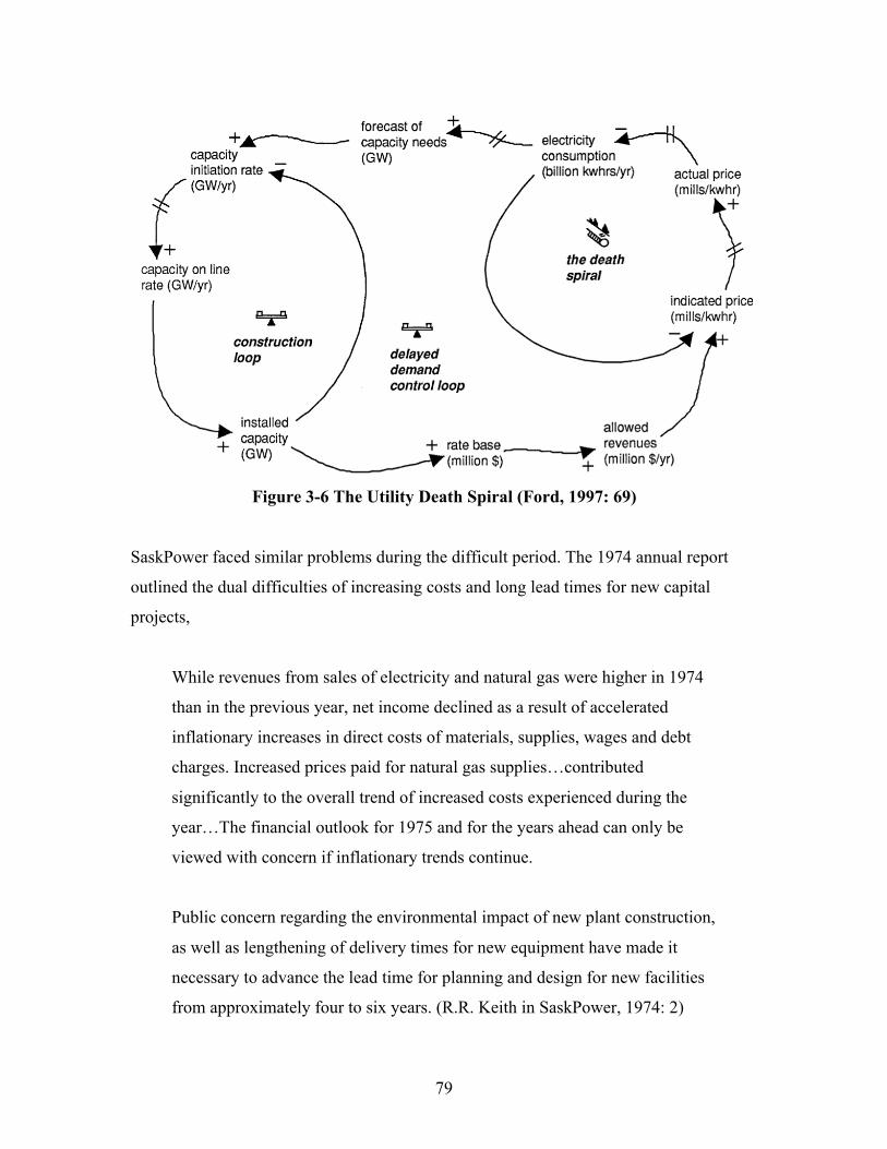
79

Figure 3-6 The Utility Death Spiral (Ford, 1997: 69)

SaskPower faced similar problems during the difficult period. The 1974 annual report

outlined the dual difficulties of increasing costs and long lead times for new capital

projects,

While revenues from sales of electricity and natural gas were higher in 1974

than in the previous year, net income declined as a result of accelerated

inflationary increases in direct costs of materials, supplies, wages and debt

charges. Increased prices paid for natural gas supplies…contributed

significantly to the overall trend of increased costs experienced during the

year…The financial outlook for 1975 and for the years ahead can only be

viewed with concern if inflationary trends continue.

Public concern regarding the environmental impact of new plant construction,

as well as lengthening of delivery times for new equipment have made it

necessary to advance the lead time for planning and design for new facilities

from approximately four to six years. (R.R. Keith in SaskPower, 1974: 2)

80

Rather than risk an investment in nuclear SaskPower opted instead to continue to do what

it knew best. The coal-fired Poplar River facility was approved in 1974 with scheduled

completion in 1979 (SaskPower, 1975).

SaskPower continued to revisit the “nuclear option” in the decades to come. A 1981 study

mentioned nuclear fusion as a technology likely to reach technical viability by 1990 and

commercial viability by 2000 (SaskPower, 1981a). But fusion has stubbornly remained a

horizon-technology; always on the horizon, never reaching technical viability.

The 1991 Saskatchewan Electrical Energy Options Review Panel (SEEORP, 1991)

included nuclear fission as an option for Saskatchewan’s electricity future and

recommended “a broad and thorough public review of nuclear power generation in

Saskatchewan including short- and long-term nuclear waste disposal” (p. 3).

In that same year, a report prepared for AECL outlined the benefits of nuclear power in

the province (AECL, 1991). Nuclear power would provide electricity that was cleaner

than coal, didn’t require flooding like hydroelectric dams, and was reliable. The AECL

(1991) report is notable because it tied nuclear power to the uranium mining industry,

outlining the “synergies” that could be developed in Saskatchewan. Similar logic would

appear in the 2009 UDP report, leading some to ask whether the UDP had simply

republished the old AECL report 18 years later.

AECL (1991) also promised that nuclear power could provide an economic development

stimulus in Saskatchewan,

As a prototype project, the Saskatchewan Candu-3 reactor could demonstrate

the benefits and advantages of its technology as the basis for a new,

Saskatchewan-based export-oriented industry. For instance, the demonstrated

success of the project in Saskatchewan would help to sell the technology in

other areas of the world with similar electrical energy needs.

(AECL, 1991: 27)

81

What was good for AECL, it appeared, was good for Saskatchewan.

Two years after the AECL (1991) and SEEORP (1991) reports SaskPower obtained a

report written by two east-coast economists commenting on the lessons Saskatchewan

could learn from New Brunswick’s Point Lepreau I project (Locke & Townley, 1993).

The Point Lepreau I power plant was of interest to Saskatchewan since New Brunswick

had a similarly sized grid. It was also an example of the risks of building a nuclear power

plant. Locke and Townley (1993) describe the project,

The construction of the first of two planned 630-megawatt CANDU reactors

began in 1974 and was brought into commercial operation 105 months later,

three years behind schedule. As well, the cost of constructing this reactor was

between two to three times higher than the original estimates.20

(Locke and Townley, 1993: 3)

Cost over-runs on the project were attributed to “‘cost plus’ and ‘cost reimbursable’

contracts” that allowed suppliers to bill more than original estimates (Locke and

Townley, 1993: 27). Locke and Townley (1993) warned SaskPower to steer clear of these

sorts of contracts.

Locke and Townley (1993) also cautioned that locals in New Brunswick were

disappointed that the construction of the plant didn’t lead to as many new jobs as

promised. Instead, more senior power union members were hired from outside the

community. Locke & Townley concluded, “The major lesson for Saskatchewan is,

therefore, to learn from Lepreau I’s mistakes” (1993: 27).

Despite their warnings, Locke & Townley (1993) also spoke of the potential

“moderating” influence of nuclear power on electricity prices in New Brunswick. This

potential upside kept the nuclear conversation open in Saskatchewan. SaskPower

explored the feasibility of nuclear in the following year with a report from the Energy

20 The second planned reactor, Lepreau II, was never built.

82

Research Group (ERG, 1994). The ERG report provided detailed cost estimates for a

CANDU-3 450-megawatt reactor. The cost estimates were based on AECL supplied data,

but were scaled (generally up) after comparison to real-world, measured performance at

plants like Point Lepreau in New Brunswick. On a levelized basis the AECL data

suggested electricity costs of 2.8-2.9 cents/kilowatt-hour (1994 $CDN) while the revised

figures were 2.8-3.7 cents/kilowatt-hour (author’s calculations; ERG, 1994).21

The Energy Research Group (ERG) report also estimated the amount of used fuel the

plant would create, the likely radiation-linked health impacts of operating the plant, and

the potential damage the would result from a catastrophic event. A quick release nuclear

accident was predicted to cause 92 health “effects” and $1 billion in property damage

(1994 $CDN). The Energy Research Group explained, “The primary reason why the

consequences of a catastrophic accident are relatively small is the low population density

that would surround a CANDU 3 in Saskatchewan” (1994: 32). In contrast, a similar

event would cause 1700 health effects in a densely populated region like New York

(ERG, 1994). This would likely be small comfort to those living near a Saskatchewan

nuclear accident site.

SaskPower continued to keep an eye on nuclear power during John Wright’s 1999-2004

tenure as SaskPower CEO.22 At that time a nuclear investment was found wanting. John

Wright commented on the continued interest in nuclear in a recent interview,

I get a kick out of the nuclear debate, because we’d done a fair amount of

look-see while I was there. I’m not averse to a nuke, if you can show me the

21 In today’s currency the ERG cost estimates would range from 4.1 – 5.3 cents/kwh (author’s calculation using Canada all-items CPI). 22 Nuclear also remained on the table during Pat Youzwa’s 2004-2008 tenure as SaskPower CEO. During this time SaskPower conducted another “preliminary siting assessment” for a nuclear reactor (SaskPower, 2007a) and drafted an internal document outlining “would it would take” to make a nuclear reactor feasible in Saskatchewan (SaskPower, 2007b). In the siting document Lake Diefenbaker, the source of 40% of Saskatchewan’s drinking water, was selected as the most desirable site due to proximity to load and availability of cooling water (SaskPower, 2007a).

83

economics of it work in an all-in basis, considering carbon at $20, $40, $100

(a tonne). Mathematically it just didn’t work; economically it didn’t work.

There was no business case for it. The government changes and ‘oh sure

there’s a business case’. An awful lot of money has been spent pursuing what

I call ‘the nuclear dream’, ‘Oh it’s right around the corner’. And now they’re

talking the smaller units. It’s not there, the structure, the nature, the size of

demand or generating capacity here, you just can’t economically do a nuke.

So frankly I just wish they’d stop it and put their money into other forms of

generation that I think down the road will pay off bigger.23

(John Wright, 2014)

As Wright alludes to, besides the challenge of high costs, SaskPower faces technical

barriers to building a nuclear reactor in Saskatchewan. In a 2006 presentation SaskPower

outlined that a nuclear reactor would pose significant problems for the Saskatchewan grid

(SaskPower, 2006a). At that time the only “economical” units on offer were 1000 MW

reactors, but SaskPower’s grid was designed so that the largest generating assets have a

capacity of about 300 MW. A large, 1000 MW reactor would cause several problems for

SaskPower. (SaskPower, 2006a)

First, a 1000 MW reactor would be sized bigger than any single load center and would

require new transmission lines for distribution around the province. (SaskPower, 2006a)

Second, a 1000 MW reactor would require SaskPower to build larger interconnections

with Manitoba and North Dakota to ensure adequate reserve margins. SaskPower is

“synchronously” connected to these jurisdictions and the entire eastern grid. When a unit

is forced to shut down in Saskatchewan, the power is instantly backed up through the

interconnections. With the introduction of a 1000 MW unit SaskPower would require a

“300% plus increase in interconnection capability” and would “likely require new 500 kV

23 During his tenure as CEO Wright focused on diversifying SaskPower’s generation fleet with investments in cogeneration, combined cycle natural gas generation, and the SaskPower’s first wind turbines.

84

transmission for interconnection reinforcement” (SaskPower, 2006a: 6). The bill for this

was estimated to be about $700 million (2006 $CDN) (SaskPower, 2006a: 6).

SaskPower (2006a) concluded that a reactor would only make sense in Saskatchewan if it

were built primarily or even exclusively to export power. This was the same conclusion

reached in a confidential internal report written in 2007; the Saskatchewan electricity

system could not host a large (750 MW plus) reactor on its own. Even a medium reactor

(361-750 MW) would require substantial export to Alberta. Only a small reactor (10-360

MW) could be integrated into the existing Saskatchewan grid. (SaskPower, 2007b)

The UDP report of 2009 targeted the construction of large reactors, but with an expected

partnership to sell electricity to Alberta. The report suggested that up to 3000 MW of

nuclear could be built close to the Alberta border so that 2000 MW of power could be

exported to the Alberta grid (UDP, 2009). Problematically, Alberta’s electricity system

runs on a different phase than Saskatchewan and Manitoba. The power would have to be

converted from AC to DC and back to AC on the Alberta side, or kept completely

separate from the Saskatchewan grid (Interview 8). It is also unclear what price nuclear

power from Saskatchewan would fetch in Alberta’s de-regulated electricity market. As a

must-run generation source a Saskatchewan nuclear plant would have to bid low to sell

into the Alberta market. The economic return of this scenario was not made clear in the

UDP report.

The UDP report also encouraged Saskatchewan to “‘follow Ontario’s lead’ in selecting a

reactor vendor and contractor for the new build project” to avoid “first-of-a-kind” risks

trying out an untested technology (UDP, 2009: 68). Ontario was widely expected to

invest in new “third generation” nuclear plants and in 2009 issued a call for proposals

requesting bids. Recognizing the substantial cost over-runs that had plagued the nuclear

industry in the past Ontario required that bids include all of the costs; there would be no

‘cost-plus’ arrangements in this round of construction. Ontario received only one bid

compliant with their guidelines; a $26 billion dollar bid from AECL to build two 1200

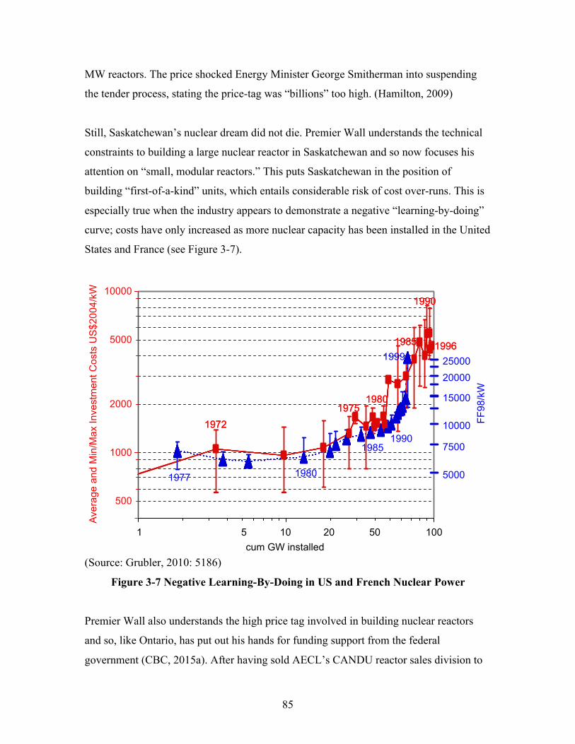
85

MW reactors. The price shocked Energy Minister George Smitherman into suspending

the tender process, stating the price-tag was “billions” too high. (Hamilton, 2009)

Still, Saskatchewan’s nuclear dream did not die. Premier Wall understands the technical

constraints to building a large nuclear reactor in Saskatchewan and so now focuses his

attention on “small, modular reactors.” This puts Saskatchewan in the position of

building “first-of-a-kind” units, which entails considerable risk of cost over-runs. This is

especially true when the industry appears to demonstrate a negative “learning-by-doing”

curve; costs have only increased as more nuclear capacity has been installed in the United

States and France (see Figure 3-7).

(Source: Grubler, 2010: 5186)

Figure 3-7 Negative Learning-By-Doing in US and French Nuclear Power

Premier Wall also understands the high price tag involved in building nuclear reactors

and so, like Ontario, has put out his hands for funding support from the federal

government (CBC, 2015a). After having sold AECL’s CANDU reactor sales division to

ARTICLE IN PRESS

combined cycles with carbon capture and sequestration (or verylarge-scale solar plants in desert areas) would be primecandidates as well.

Lastly, the French nuclear case has also demonstrated the limits ofthe learning paradigm: the assumption that costs invariably decreasewith accumulated technology deployment. The French exampleserves as a useful reminder of the limits of the generalizability ofsimplistic learning/experience curve models. Not only do nuclearreactors across all countries with significant programs invariablyexhibit negative learning, i.e., cost increase rather than decline, butthe pattern is also quite variable, defying approximations by simplelearning-curve models, as shown in Fig. 13.

First of all, Fig. 13 provides a useful reminder on the dangers of‘‘logarithmic compression’’ in the customary double log learningcurve representations. Despite the learning curve metaphor isclearly not applicable in the case of nuclear in both the US andFrance illustrating the limits of simplistic learning curve assump-tions in technology studies and policy models, the model none-theless allows an additional insight. The rhythm (as opposed tothe different rates and extent) of cost escalation between the twocountries appears strikingly similar. Initially, cost escalations arepositive, but modest until a threshold value of some 20 GWinstalled capacity is reached, followed by a phase of acceleratedcost escalation to another threshold level at some 40–50 GW,beyond which cost escalation simply skyrockets. At this stageabove observation remains entirely conjectural. Further evidencefrom more country studies (and disclosure of reactor specific costsdata for France to improve upon the estimates presented here) areneeded before above conjecture can be moved to the status of ahypothesis and explanatory factors explored. However, it seemsnot implausible to speculate about the existence of non-linearthreshold effects in the economics of large-scale complextechnology systems that however in the case of nuclear(as opposed to ITC) work in the opposite direction (i.e. costsincrease rather than decrease).

In symmetry to the often evoked ‘‘learning-by-doing’’ phe-nomenon, there appears not only to be ‘‘forgetting by not doing’’18

(Rosegger, 1991) but also ‘‘forgetting by doing’’, suggesting thattechnology learning possibilities are not only structured by theactors and institutional settings involved, but are also a funda-mental characteristic of technologies themselves.

In the case of nuclear, a theoretical framework explaining thisnegative learning was discussed by Lovins (1986: 17–21) whoreferred to the underlying model as Bupp–Derian–Komanoff–Taylor hypothesis. In essence, the model suggests that withincreasing application (‘‘doing’’), the complexity of the technologyinevitably increases leading to inherent cost escalation trends thatlimit or reverse ‘‘learning’’ (cost reduction) possibilities. Inother words, technology scale-up can lead to an inevitableincrease in systems complexity (in the case of nuclear, fullfuel cycle management, load-following operation mode, andincreasing safety standards as operation experience [and unanti-cipated problems] are accumulating) that translates into real-cost

Aver

age

and

Min

/Max

Inve

stm

ent C

osts

US$

2004

/kW

FF98

/kW

19721975

1985

1980

1990

1996

100101cum GW installed

10000

500

5000

1000

2000

5000

20000

15000

10000

7500

25000

205

19721975

1985

1980

1990

1996

19901985

19801977

1999

50

Fig. 13. Average and min/max reactor construction costs per year of completion date (cf. Fig. 12 above) for US and France versus cumulative capacity completed.

Table A1Average specific French nuclear reactor construction costs inferred from annualexpenditures. Best guess and min/max values for two uncertainty ranges (in 1000FF98 per kW).

1000 FF98/kW Best guess Min-1 Max-1 Min-2 Max-2

Pre-1973 avg 6.31 5.69 6.31 3.94 7.611974 4.23 4.01 4.23 2.88 4.841975 4.45 4.21 4.45 3.75 4.891976 4.42 4.04 4.42 4.01 5.301977 4.38 4.14 4.38 4.07 5.821978 5.16 4.72 5.16 4.70 5.831979 6.32 5.88 6.32 4.93 6.671980 6.91 6.57 6.91 5.88 7.071981 6.80 6.54 6.80 6.39 8.371982 6.89 6.74 6.89 6.58 9.281983 8.03 7.27 8.04 6.90 9.051984 7.03 7.03 7.13 6.63 7.141985 7.83 7.83 8.03 6.58 8.101986 8.73 8.65 8.85 7.19 8.891987 9.78 9.78 10.23 8.88 10.261988 11.47 11.43 11.72 10.93 11.831989 11.40 11.40 11.65 10.39 12.351990 10.01 10.01 10.66 7.19 10.79Post 1990 average 14.54 13.76 14.68 12.22 14.74

18 Cost escalation as a result of knowledge depreciation/obsolescence and/orerosion institutional capability.

A. Grubler / Energy Policy 38 (2010) 5174–51885186

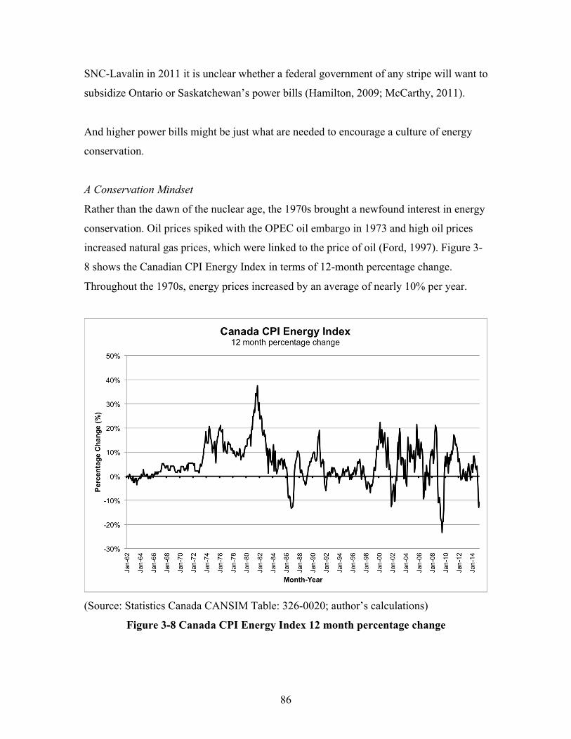
86

SNC-Lavalin in 2011 it is unclear whether a federal government of any stripe will want to

subsidize Ontario or Saskatchewan’s power bills (Hamilton, 2009; McCarthy, 2011).

And higher power bills might be just what are needed to encourage a culture of energy

conservation.

A Conservation Mindset

Rather than the dawn of the nuclear age, the 1970s brought a newfound interest in energy

conservation. Oil prices spiked with the OPEC oil embargo in 1973 and high oil prices

increased natural gas prices, which were linked to the price of oil (Ford, 1997). Figure 3-

8 shows the Canadian CPI Energy Index in terms of 12-month percentage change.

Throughout the 1970s, energy prices increased by an average of nearly 10% per year.

(Source: Statistics Canada CANSIM Table: 326-0020; author’s calculations)

Figure 3-8 Canada CPI Energy Index 12 month percentage change

87

Energy price increases in the 1970s translated into inflation across the board (See Figure

3-5) and utilities experienced the “difficult period” of increasing costs and construction

delays mentioned above (Ford, 1997).

Meanwhile, people like Amory Lovins argued that a “soft path” of energy conservation

and decentralized renewable energy offered a more desirable future than the “hard path”

of demand growth and big, centralized generation projects like nuclear plants (Lovins,

1976). Utilities began to rethink their business models.

Prior to this period, the goal in Saskatchewan had been to promote electricity demand,

not constrain it. In 1928, the SPRC advocated “an active sales campaign” to increase the

use of “domestic electric utensils” (i.e. household appliances) and expand demand for

electricity (SPRC, 1928: 113).

The story was much the same in at the newly founded SaskPower Corporation in 1950,

The success of the electric utility depends on the full use of the service by the

customer. Much more promotion on electrical use, including greater

purchases of electrical equipment and appliances for our customers, is

required if electrical consumptions in this Province are to compare with those

of other provinces. Studies, commenced during the year, on load growths and

customer usage are continuing in an attempt to make electrical service more

attractive to customers. (SaskPower, 1950: 4)

SaskPower designed travelling roadshows to promote the “the advantage of electrical

living” (SaskPower, 1951: 7) and appointed a female spokesperson they called ‘Penny

Powers’ to share the good news about the advantages of electricity (see Figure 3-9).

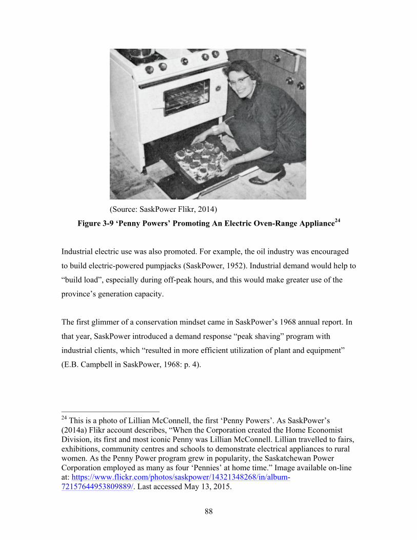
88

(Source: SaskPower Flikr, 2014)

Figure 3-9 ‘Penny Powers’ Promoting An Electric Oven-Range Appliance24

Industrial electric use was also promoted. For example, the oil industry was encouraged

to build electric-powered pumpjacks (SaskPower, 1952). Industrial demand would help to

“build load”, especially during off-peak hours, and this would make greater use of the

province’s generation capacity.

The first glimmer of a conservation mindset came in SaskPower’s 1968 annual report. In

that year, SaskPower introduced a demand response “peak shaving” program with

industrial clients, which “resulted in more efficient utilization of plant and equipment”

(E.B. Campbell in SaskPower, 1968: p. 4).

24 This is a photo of Lillian McConnell, the first ‘Penny Powers’. As SaskPower’s (2014a) Flikr account describes, “When the Corporation created the Home Economist Division, its first and most iconic Penny was Lillian McConnell. Lillian travelled to fairs, exhibitions, community centres and schools to demonstrate electrical appliances to rural women. As the Penny Power program grew in popularity, the Saskatchewan Power Corporation employed as many as four ‘Pennies’ at home time.” Image available on-line at: https://www.flickr.com/photos/saskpower/14321348268/in/album-72157644953809889/. Last accessed May 13, 2015.

89

The 1970s saw this conservation mindset expand. As the 1974 Annual Report described,

The Corporation has stepped up its public information program emphasizing

the wise and efficient use of energy. Through advertisements in newspapers

and on radio and television, customers are being encouraged to reduce cost

and conserve energy resources by using energy wisely. (SaskPower, 1974: 2)

Penny Power had been transformed into Penny-Pincher.

In 1979 SaskPower formalized its promotion of energy conservation by establishing “an

Energy Conservation Division to encourage wise and efficient use of energy in the home,

farm, business and industry” (SaskPower, 1979: 13). A series of conservation programs

followed in years to come (See Table 3-3).

These energy conservation and demand-side management programs have undoubtedly

helped to reduce electricity demand in Saskatchewan. Problematically these programs are

not well integrated with supply planning; instead of being under the management of the

Supply Planning Department, DSM programs are run out of the Customer Services

branch of SaskPower. Their appeal as a marketing exercise is likely as or more important

than the savings they generate.

This separation of supply planning and Demand Side Management (DSM) precludes

electricity conservation from reaching its full potential. The current target for DSM at

SaskPower is to save or shift enough demand to prevent 100 MW of capacity

construction by 2018. The technical potential for DSM savings in Saskatchewan may be

closer to 400-450 MW, while 300 MW is considered an achievable, albeit more

aggressive, target (Interview 12).

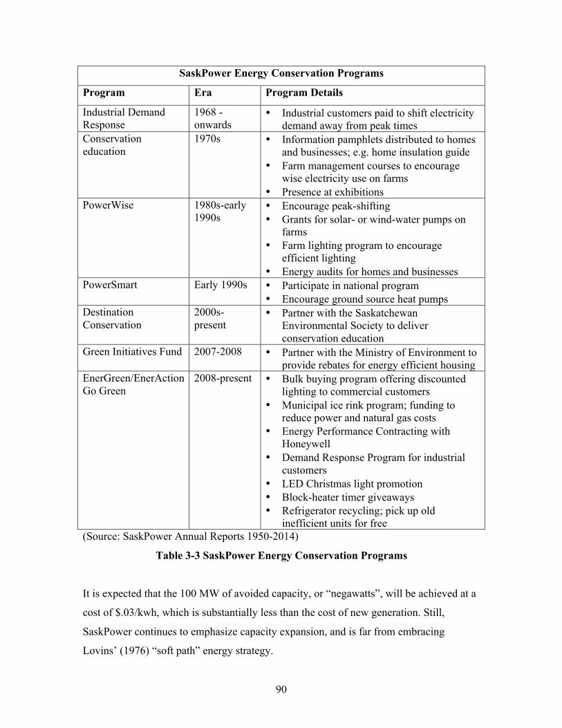
90

SaskPower Energy Conservation Programs

Program Era Program Details

Industrial Demand Response

1968 - onwards

• Industrial customers paid to shift electricity demand away from peak times

Conservation education

1970s • Information pamphlets distributed to homes and businesses; e.g. home insulation guide

• Farm management courses to encourage wise electricity use on farms

• Presence at exhibitions PowerWise 1980s-early

1990s • Encourage peak-shifting • Grants for solar- or wind-water pumps on

farms • Farm lighting program to encourage

efficient lighting • Energy audits for homes and businesses

PowerSmart Early 1990s • Participate in national program • Encourage ground source heat pumps

Destination Conservation

2000s-present

• Partner with the Saskatchewan Environmental Society to deliver conservation education

Green Initiatives Fund 2007-2008 • Partner with the Ministry of Environment to provide rebates for energy efficient housing

EnerGreen/EnerAction Go Green

2008-present • Bulk buying program offering discounted lighting to commercial customers

• Municipal ice rink program; funding to reduce power and natural gas costs

• Energy Performance Contracting with Honeywell

• Demand Response Program for industrial customers

• LED Christmas light promotion • Block-heater timer giveaways • Refrigerator recycling; pick up old

inefficient units for free (Source: SaskPower Annual Reports 1950-2014)

Table 3-3 SaskPower Energy Conservation Programs

It is expected that the 100 MW of avoided capacity, or “negawatts”, will be achieved at a

cost of $.03/kwh, which is substantially less than the cost of new generation. Still,

SaskPower continues to emphasize capacity expansion, and is far from embracing

Lovins’ (1976) “soft path” energy strategy.

91

A confounding factor for DSM is the state of Saskatchewan’s electricity grid. For DSM

to reach its full potential smart grid technology is key. With a smart grid appliances can

be set to respond to the relative availability (or price) of electricity; for example, air

conditioners can be cycled on and off throughout the grid to flatten peak demand on hot

summer days. This would allow SaskPower to shave peak electricity demand and delay

capacity expansions.

Saskatchewan started on the path to a smart grid in 2010 (see Figure 3-10). Between the

fall of 2013 and the summer of 2014 108,000 smart meters were installed in the province.

Concerns arose in late June 2014 when several smart meters “failed catastrophically” by

either melting or burning (CIC, 2014: 2). By the end of July the count of failed smart

meters was up to eight. The provincial cabinet responded by ordering all of the installed

smart meters removed (CIC, 2014). The removal of Saskatchewan’s smart meters was

nearly complete by February 2015 at a cost of $15 million (CKOM, 2015).

Political columnist Murray Mandryk compared the smart meter “fiasco” to the Channel

Lake scandal (see footnote 14). In a prescient column on September 10, 2014 Mandryk

noted that “heads rolled” at SaskPower after Channel Lake. The Crown Investment

Corporation (CIC), the umbrella organization in charge of Saskatchewan’s Crowns,

published its review of the smart meters affair on October 27, 2014 and found that

“customer safety was not given enough of a priority” (CIC, 2014a). SaskPower CEO

Robert Watson resigned that day (Clancy, 2014). A smart grid for Saskatchewan will now

have to wait until the memory of smoking meters fades into history.

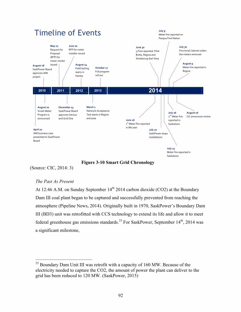
92

Figure 3-10 Smart Grid Chronology

(Source: CIC, 2014: 3)

The Past As Present

At 12:46 A.M. on Sunday September 14th 2014 carbon dioxide (CO2) at the Boundary

Dam III coal plant began to be captured and successfully prevented from reaching the

atmosphere (Pipeline News, 2014). Originally built in 1970, SaskPower’s Boundary Dam

III (BD3) unit was retrofitted with CCS technology to extend its life and allow it to meet

federal greenhouse gas emissions standards.25 For SaskPower, September 14th, 2014 was

a significant milestone,

25 Boundary Dam Unit III was retrofit with a capacity of 160 MW. Because of the electricity needed to capture the CO2, the amount of power the plant can deliver to the grid has been reduced to 120 MW. (SaskPower, 2015)

Smart Meter Review | 3

Timeline of Events

2010 2011 2012 2013 2014

April 20 AMI business case presented to SaskPower Board

August 18 SaskPower Board approves AMI project

August 20 Smart Meter Program is announced

December 15 SaskPower Board approves Sensus and Grid One

August 24 Field testing starts in Hanley

March 1 Network Acceptance Test starts in Regina and area

October 17 Full program roll out

June 16 1st Meter fire reported in McLean

June 30 3 Fires reported: Pilot Butte, Regina and Strasbourg-Earl Grey

July 10 SaskPower stops installations

July 9 Meter fire reported on Pasqua First Nation

July 13 Meter fire reported in Saskatoon

July 26 2nd Meter fire reported in Saskatoon

August 9 Meter fire reported in Regina

August 16 CIC announces review

May 27 Request for Proposal (RFP) for meter vendor issued

July 30 Provincial Cabinet orders the meters removed

June 20 RFP for meter installer issued

93

In 2014, we took a giant leap forward by delivering the world’s first

commercial-scale post-combustion carbon capture and storage (CCS) facility

at coal-fired Boundary Dam Power Station. We will capture 90% of the

carbon dioxide created by a generating unit that is capable of providing

enough power to supply 100,000 homes. Emissions will be reduced by about

1,000,000 tonnes each year, prolonging the life of an economical, stable and

secure local fuel source.

(SaskPower, 2014: 1)

The final price tag for the CCS project is $1.467 billion, which works out to

$12,225/kilowatt; a price even higher than the nuclear plants rejected by Ontario in 2009

(Zinchuk, 2015; Hamilton, 2009). Easing the burden for Saskatchewan, the federal

government contributed $240 million to the project (Mandryk, 2014a).

Further revenue will be generated by selling captured CO2 to the oil company Cenovus

for use in enhanced oil recovery (EOR). This source of revenue has set off alarms. For

every tonne of CO2 captured and injected into an oil well “about 2.7 tonnes of carbon

dioxide are eventually emitted from combustion of the oil recovered” (Banks and

Bigland-Pritchard, 2015: 17 citing figures from Wong et al, 2013). Some of the CO2

injected into the oil wells will also return to the surface when the oil is extracted (Banks

& Bigland-Pritchard, 2015).

Political columnist Murray Mandryk (2014a) has argued “the real winner” of the CCS

project is “Calgary-based Cenovus” since the company will make millions in added

revenue by injecting CO2 into its aging oil fields. Banks & Bigland-Pritchard (2015)

come to a similar conclusion, “The predominant reason for the CCS to go ahead appears

to be to recover more oil from south east Saskatchewan and reward the oil producing

companies” (p. 20).

The history of the CCS concept in Saskatchewan suggests there is some truth to these

claims. As early as 1994 SaskPower discussed “Investigating the practicality of capture

94

carbon dioxide from our coal-fired power stations for use in enhanced oil recovery”

(SaskPower, 1994: 16). The idea is mentioned again in 1995’s Annual Report where

SaskPower stated it was “Studying the potential for capture carbon dioxide from power

plants for use in enhanced oil recovery” (SaskPower, 1995: 19). Enhanced oil recovery

appears to have been part of the rationale for CCS from the beginning.

For Premier Brad Wall, the link to Enhanced Oil Recovery (EOR) is a strength of the

CCS project, “Legislators around the world view CO2 basically as a pollutant. We’re

getting paid for it in Saskatchewan because of this clean coal project. That’s a positive

thing” (Brad Wall in Pipeline News, 2014: A14).

The Premier sees CCS as providing a triple benefit by extending oil production in aging

oil wells – which in turn increases provincial royalties – saving jobs in the Estevan coal

plants, and indicating Saskatchewan’s commitment to greenhouse gas emissions

reduction. On this last point, Wall believes that Boundary Dam III will help convince the

United States government that the oil-producing provinces of Canada are environmental

stewards. This in turn can help convince the U.S. to approve the Keystone XL pipeline:

I’ve been saying, when we’re down in the United States on Keystone, even,

we should reference projects like this. This particular (U.S.) administration,

they want some environmental elbow room from the different environmental

NGOs that hate, that don’t like Keystone. They need some environmental

elbow room to quote-unquote “deal with the Canadians.” That pipeline is

definitely a deal with Canadians.

We’re able to go down, and have been going down, saying, “Look at the

project, because in your coal states it might have an application. But also look

at it as validation that we’re serious about the environment, and tell those

worried about Canada in general, they ought not to. In Canada, this is the

largest per-capita project related to CO2 mitigation.” I think it helps on that

front as well. (Brad Wall quoted in Pipeline News, 2014: A15)

95

There are other ways for Saskatchewan to improve its image in the United States that

don’t involve carbon capture and storage. Banks & Bigland-Pritchard (2015) use

calculations by James Glennie to show that an investment in wind could generate the

equivalent amount of electricity for $300 million less than the Boundary Dam project.

Mike Monea, project manager of the Boundary Dam CCS project, responded to this

critique by pointing to the variability of electricity generated by wind,

Last Sunday we hit a peak (of power consumption) at 6 p.m., suppertime. We

had one megawatt coming from our wind turbines. There was no wind

blowing. What did we use? We used coal-fired plants for the baseload, so

nobody had disruption in their power.

(Mike Monea quoted in Zinchuk, 2015)

As Monea implies, SaskPower does not plan to rely on variable renewables like wind to

replace coal-fired generation because they cannot act as reliable baseload power. This is a

perspective that resonates with the Financial Editor of the Regina LeaderPost. After the

release of the critique of CCS by Banks & Bigland-Pritchard (2015), Bruce Johnstone

wrote,

Another day, another report from an alternative energy-public policy group

slamming the $1.47-billion carbon capture and storage (CCS) project at

SaskPower’s Boundary Dam power station at Estevan.

But is it realistic to assume the world, which currently relies on coal for more

than 40 per cent of its electricity generation, can easily turn to natural gas or

renewables for its baseload power? With huge developing countries, like

China and India, still dependent on coal-fired generation, what is the

responsible alternative?

96

I submit that CCS or clean coal is one solution. It may not be a silver bullet,

but it does provide us some “breathing room,’’ while we reduce our

dependence on fossil fuels.

Wind energy is also a solution; so are solar, biomass and other renewables.

SaskPower is at 25 per cent renewable energy today and hopes to generate 10

per cent of its capacity from wind by 2020. But SaskPower needs baseload

power, like coal and natural gas-fired generation, to keep the lights on.

By definition, intermittent energy sources, like wind, can’t provide baseload

power, and it proponents are deluding themselves and the public if they think

it can.

(Johnstone, 2015a)

Interestingly, Johnstone (2015a) points to the viability of natural gas for baseload

generation. With the exception of Boundary Dam III, SaskPower appears to prefer that

route.

The Natural Gas – Wind Nexus?

Coal has been king in Saskatchewan for over fifty years. The grid was built to move

electrons generated by the “cheap lignite coal” found near Estevan and Coronach to load

centres like Regina. In interviews with SaskPower employees past and present there was

a sentiment that SaskPower possesses a “coal culture”. Generations of SaskPower

employees have spent their careers working within the coal-based system. It is little

surprise that SaskPower is exploring CCS as a way to keep coal alive in Saskatchewan.

In the past fifteen years, however, a shift has been taking place. Figure 3-11 provides a

look at Saskatchewan’s electricity generation by type from 1954-2015. This figure shows

that natural gas-fired generation has quietly been growing and electricity generated by

coal plants has stagnated and begun to decline.

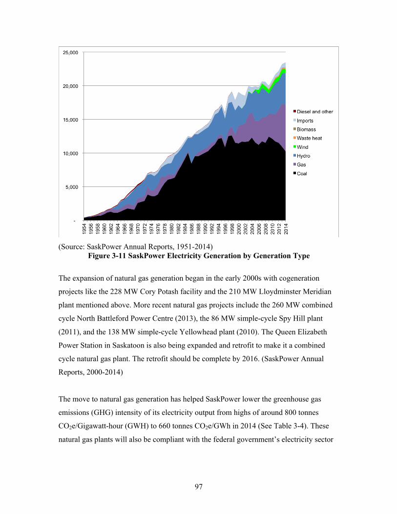
97

(Source: SaskPower Annual Reports, 1951-2014)

Figure 3-11 SaskPower Electricity Generation by Generation Type

The expansion of natural gas generation began in the early 2000s with cogeneration

projects like the 228 MW Cory Potash facility and the 210 MW Lloydminster Meridian

plant mentioned above. More recent natural gas projects include the 260 MW combined

cycle North Battleford Power Centre (2013), the 86 MW simple-cycle Spy Hill plant

(2011), and the 138 MW simple-cycle Yellowhead plant (2010). The Queen Elizabeth

Power Station in Saskatoon is also being expanded and retrofit to make it a combined

cycle natural gas plant. The retrofit should be complete by 2016. (SaskPower Annual

Reports, 2000-2014)

The move to natural gas generation has helped SaskPower lower the greenhouse gas

emissions (GHG) intensity of its electricity output from highs of around 800 tonnes

CO2e/Gigawatt-hour (GWH) to 660 tonnes CO2e/GWh in 2014 (See Table 3-4). These

natural gas plants will also be compliant with the federal government’s electricity sector

98

GHG regulations, which require all new power plants to be ‘as clean as gas’ and emit

only 420 tonnes CO2e/GWh (CEPA, 2012).

1990 2000 2005 2007 2008 2009 2010 2011 2014 Generation Intensity

(tonnes CO2e/GWh) 798 858 780 750 709 793 800 745 660

(Sources: Environment Canada, 2013; SaskPower, 2014)

Table 3-4 Saskatchewan Electricity GHG Intensity

The move is also changing the business model of SaskPower. Of the six natural gas fired

facilities built since 2000, three are privately owned (Meridian, Spy Hill, and North

Battleford), and one (Cory) involves a significant private partnership. Brad Wall has kept

his promise not to sell off Saskatchewan’s Crown Corporations, but Saskatchewan

citizens may one day wake up to realize that SaskPower has become only a system

operator and electricity distributor, not a power generator.26

The increase in natural gas-fired generation offers an effective back-up for variable wind

power. New natural gas-fired plants can ramp quickly to fill in supply when the winds die

down (Interview 2). And, as mentioned above, SaskPower values wind for its ability to

reduce the use of natural gas fuel.

The SaskPower system was home to 198 MW of utility-scale wind capacity in 2014. This

is slated to double by 2018 with the installation of a 23 MW wind farm at Morse and a

177 MW wind farm at Chaplin (SaskPower, 2014). At that time wind will comprise just

under 10% of system capacity.

Will the trend towards natural gas combined cycle generation paired with wind power

continue in Saskatchewan? Is the coal-hydro nexus being replaced with a natural gas –

wind nexus?

26 Under pressure from public sector unions and the NDP Brad Wall committed to not sell Saskatchewan’s Crown Corporations in his 2007 election campaign. The promise helped remove fear that Wall’s government would be a repeat of the Devine era.

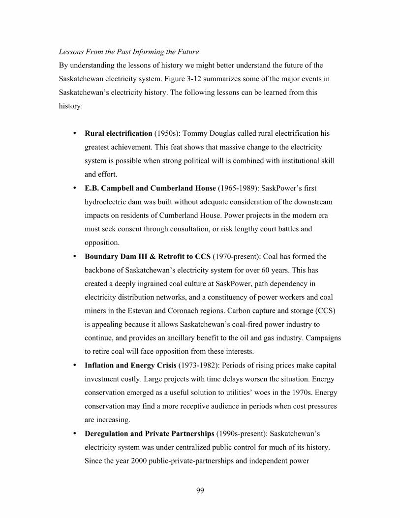
99

Lessons From the Past Informing the Future

By understanding the lessons of history we might better understand the future of the

Saskatchewan electricity system. Figure 3-12 summarizes some of the major events in

Saskatchewan’s electricity history. The following lessons can be learned from this

history:

• Rural electrification (1950s): Tommy Douglas called rural electrification his

greatest achievement. This feat shows that massive change to the electricity

system is possible when strong political will is combined with institutional skill

and effort.

• E.B. Campbell and Cumberland House (1965-1989): SaskPower’s first

hydroelectric dam was built without adequate consideration of the downstream

impacts on residents of Cumberland House. Power projects in the modern era

must seek consent through consultation, or risk lengthy court battles and

opposition.

• Boundary Dam III & Retrofit to CCS (1970-present): Coal has formed the

backbone of Saskatchewan’s electricity system for over 60 years. This has

created a deeply ingrained coal culture at SaskPower, path dependency in

electricity distribution networks, and a constituency of power workers and coal

miners in the Estevan and Coronach regions. Carbon capture and storage (CCS)

is appealing because it allows Saskatchewan’s coal-fired power industry to

continue, and provides an ancillary benefit to the oil and gas industry. Campaigns

to retire coal will face opposition from these interests.

• Inflation and Energy Crisis (1973-1982): Periods of rising prices make capital

investment costly. Large projects with time delays worsen the situation. Energy

conservation emerged as a useful solution to utilities’ woes in the 1970s. Energy

conservation may find a more receptive audience in periods when cost pressures

are increasing.

• Deregulation and Private Partnerships (1990s-present): Saskatchewan’s

electricity system was under centralized public control for much of its history.

Since the year 2000 public-private-partnerships and independent power

100

producers have become an important part of Saskatchewan’s electricity system.

The SaskPower business model of keeping electricity rates low through average

cost pricing remains, but at some point SaskPower may find itself to be little

more than an electricity distribution company. This may have implications for the

nature of the grid; private interests are unlikely to pursue expensive generation

technologies such as small, modular nuclear reactors or carbon capture and

storage (CCS). To date independent power producers have been building

cogeneration facilities, natural gas plants, and wind farms.

• GHG Regulation (2012-present): The federal government’s coal-fired electricity

regulations have placed an expiry date on Saskatchewan’s coal plants. They must

either be shuttered or retrofit with CCS at the end of their life expectancy.

SaskPower will be forced to make decisions on expanding the CCS project to

include Boundary Dam IV and V within the next few years. If SaskPower

decides to retrofit those plants to CCS they will then have until 2025 to make the

transition. If they decide not to retrofit the plants they must be shuttered by 2019

(CEPA, 2012). Yet, the high cost of Boundary Dam III makes continued

investments in CCS politically risky. Will SaskPower allow coal to wither in

Saskatchewan?

With these lessons from history in mind this dissertation explores scenarios for the future

of Saskatchewan’s electricity system. The history of the system has been filled with

intrigue, rolling heads, and Canadian firsts. Where will the future lead?

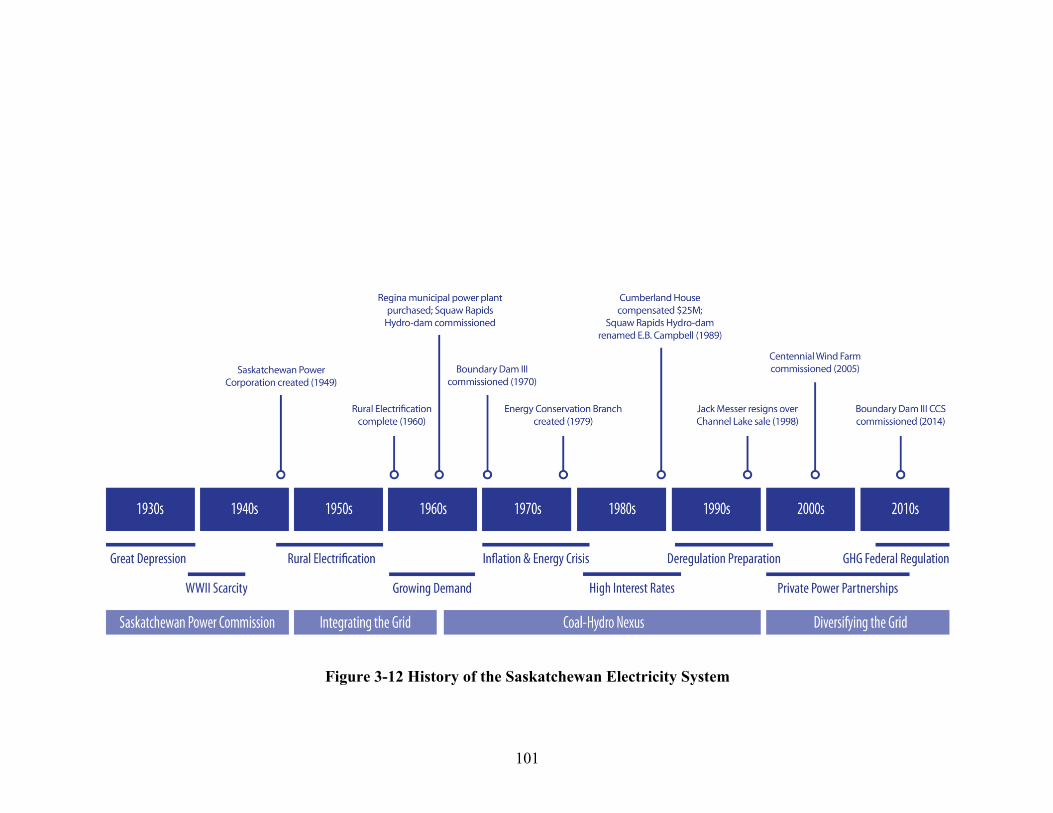
101

Figure 3-12 History of the Saskatchewan Electricity System

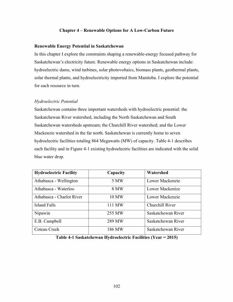
102

Chapter 4 – Renewable Options for A Low-Carbon Future

Renewable Energy Potential in Saskatchewan

In this chapter I explore the constraints shaping a renewable-energy focused pathway for

Saskatchewan’s electricity future. Renewable energy options in Saskatchewan include:

hydroelectric dams, wind turbines, solar photovoltaics, biomass plants, geothermal plants,

solar thermal plants, and hydroelectricity imported from Manitoba. I explore the potential

for each resource in turn.

Hydroelectric Potential

Saskatchewan contains three important watersheds with hydroelectric potential: the

Saskatchewan River watershed, including the North Saskatchewan and South

Saskatchewan watersheds upstream; the Churchill River watershed; and the Lower

Mackenzie watershed in the far north. Saskatchewan is currently home to seven

hydroelectric facilities totaling 864 Megawatts (MW) of capacity. Table 4-1 describes

each facility and in Figure 4-1 existing hydroelectric facilities are indicated with the solid

blue water drop.

Hydroelectric Facility Capacity Watershed

Athabasca - Wellington 5 MW Lower Mackenzie

Athabasca - Waterloo 8 MW Lower Mackenize

Athabasca - Charlot River 10 MW Lower Mackenzie

Island Falls 111 MW Churchill River

Nipawin 255 MW Saskatchewan River

E.B. Campbell 289 MW Saskatchewan River

Coteau Creek 186 MW Saskatchewan River

Table 4-1 Saskatchewan Hydroelectric Facilities (Year = 2015)

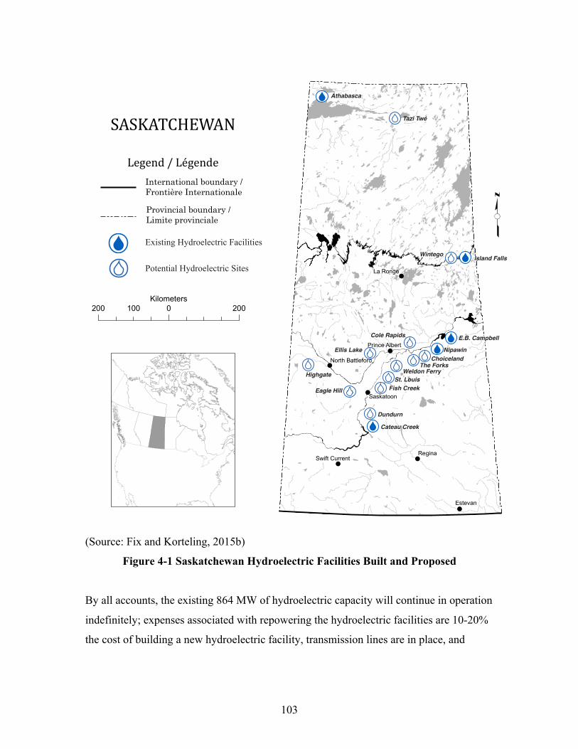
103

(Source: Fix and Korteling, 2015b)

Figure 4-1 Saskatchewan Hydroelectric Facilities Built and Proposed

By all accounts, the existing 864 MW of hydroelectric capacity will continue in operation

indefinitely; expenses associated with repowering the hydroelectric facilities are 10-20%

the cost of building a new hydroelectric facility, transmission lines are in place, and

!

!!

!

!

!

!

Regina

Estevan

La Ronge

Saskatoon

Prince Albert

Swift Current

North Battleford

tLegend / Légende

200 0 200100Kilometers

SASKATCHEWAN

International boundary / Frontière Internationale

Provincial boundary / Limite provinciale

E.B. Campbell

Nipawin

Cateau Creek

Island FallsWintego

Eagle Hill

Choiceland

The Forks

Weldon Ferry

St. Louis

Fish Creek

Dundurn

Highgate

Ellis Lake

Cole Rapids

Existing Hydroelectric Facilities

Potential Hydroelectric Sites

Athabasca

Tazi Twé

104

hydroelectric power does not release greenhouse gas emissions (GHGs) through the

combustion of fossil fuels.27

The potential for expanding hydroelectric power has been explored several times

throughout Saskatchewan’s history. As outlined in Chapter 3 (See Figure 3-4), David

Cass-Beggs (1960) sketched out a plan for a series of hydroelectric dams along the South

Saskatchewan and Saskatchewan Rivers. At that time, SaskPower was preparing to build

the E.B. Campbell facility (then called Squaw Rapids). The Coteau Creek (1969) and

Nipawin (1986) facilities were later completed in accordance with Cass-Beggs’

hydroelectric plan.

Future hydroelectric potential in Saskatchewan varies by watershed. In the Saskatchewan

River watershed there is potential for dams at the Forks and Choiceland (See Figure 4-1).

A dam at the Forks could contain “five 84 MW units” equaling 420 MW total output,

while a dam at Choiceland could host “four 75 MW units”, creating 300 MW of output

(McClement and Campbell, 1977: 51). There is also potential to install two additional 84

MW units at Nipawin to increase capacity at that station from 255 MW to over 420 MW

(McClement and Campbell, 1977). In total this represents a potential to double the

current hydroelectric capacity in the province on the Saskatchewan River alone.

There is also potential to expand hydroelectric potential on the Churchill River. As

outlined in Chapter 3, SaskPower proposed to build a 300 MW hydroelectric dam at the

Wintego site on the Churchill River in 1973. This proposal was met with stiff opposition

from Saskatchewan First Nations and was rejected by the Churchill River Board of

27 There are, however, GHG emissions associated with flooding land to create a hydroelectricity facility. Barros et al. (2011) estimated that the sum total of annual emissions from the world’s hydroelectric reservoirs is approximately 58 Megatonnes (Mt) as carbon dioxide (CO2) and 3 Mt as methane (CH4) from the reservoir surface. Adding the action of turbines and river outflow increases this estimate roughly twofold. Lakes and streams generally, unless they are eutrophic, release CO2 and CH4. Releases of GHGs from hydroelectric reservoirs are greatest in tropical regions and lower in temperate and boreal forest regions. (Barros et al., 2011)

105

Inquiry (CRBI, 1978; Waldram, 1993). This lack of “social license” poses a barrier for

future hydroelectric development on the Churchill.

SaskPower is having better success obtaining social license for the Tasi Twé

hydroelectric project in the far north of Saskatchewan, near Black Lake. Formerly called

the Elizabeth Falls project, the Tasi Twé project is a partnership between SaskPower and

the local Black Lake First Nation (Golder and Associates, 2012). If successful the Tasi

Twé project will result in the creation of a 42-50 MW hydroelectric facility on the Black

Lake River in the Lower Mackenzie watershed. Other small hydroelectric projects could

be built in the watershed to provide a total of 323 MW of additional capacity. These

northern dams are, however, quite expensive to build. The most affordable are likely in

the range of $11,000-15,000/kilowatt capital cost, while the most expensive may cost as

much as $30,000/kw to build (Interview 17).

Watershed Existing Potential Additions Total

Saskatchewan River 730 MW 1000 MW 1730 MW

Churchill River 111 MW 480 MW 591 MW

Lower Mackenzie 23 MW 300 MW 323 MW

Total 864 MW 1780 MW 2644 MW

Table 4-2 Potential Hydroelectric Capacity

In total, there is potential to add up to 1780 MW of additional hydroelectric capacity in

Saskatchewan, which would bring the provincial total to 2644 MW.

Wind Power

Residents of Saskatchewan know very well the strength and frequency of prairie winds.

Though the bane of winter existence in the province, these winds provide an opportunity

for near zero-carbon electricity generation.28 Figure 4-2 provides a look at the wind

28 Note that while wind turbines do not emit greenhouse gas emissions (GHGs) directly in their operation, emissions are generated in the process of manufacturing, installing,

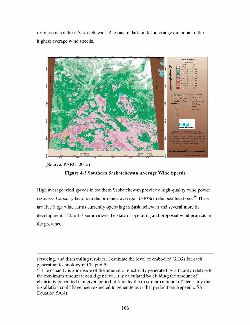
106

resource in southern Saskatchewan. Regions in dark pink and orange are home to the

highest average wind speeds.

(Source: PARC, 2015)

Figure 4-2 Southern Saskatchewan Average Wind Speeds

High average wind speeds in southern Saskatchewan provide a high-quality wind power

resource. Capacity factors in the province average 36-40% in the best locations.29 There

are five large wind farms currently operating in Saskatchewan and several more in

development. Table 4-3 summarizes the state of operating and proposed wind projects in

the province.

servicing, and dismantling turbines. I estimate the level of embodied GHGs for each generation technology in Chapter 9. 29 The capacity is a measure of the amount of electricity generated by a facility relative to the maximum amount it could generate. It is calculated by dividing the amount of electricity generated in a given period of time by the maximum amount of electricity the installation could have been expected to generate over that period (see Appendix 5A Equation 5A.4).

107

(Source: Reproduced with permission from SaskWind, 2015)

Table 4-3 Wind Power Projects in Saskatchewan

SaskPower has committed to having wind power contribute 10% of provincial electricity

generation capacity by 2020 (Mohr, 2015).30 By 2019 217 MW of additional wind

capacity will be installed, including a 177 MW wind farm near Chaplin and a 20 MW

wind farm at Riverhurst – both located in the vicinity of Moose Jaw, and a 20 MW

project at Grenfell, which is located 126 km east of Regina. An additional 100 MW of

wind power will be developed to meet the 2020 target (Mohr, 2015; SaskWind, 2015).

SaskPower has also made the commitment that by 2030 wind will compose 20% of total

electricity generating capacity or approximately 1000-1100 MW (Mohr, 2015). Meeting

the 2030 target will require another 500-600 MW of wind power in the decade between

2020-2030 (SaskWind, 2015). This represents a change in plans for SaskPower. Former

CEO Robert Watson stated in 2013 that wind would “not in our lifetime” compose more

than 8% capacity in the province (StarPhoenix quoted by SaskWind, 2015). SaskPower’s

new CEO Mike Marsh appears to be more favourable towards the technology.

In a regional context SaskPower’s goals appear eminently achievable. Neighbouring

North Dakota had 1886 MW of wind capacity installed at the end of 2014, which

provided 17.6% of total electricity generated in that state (U.S. DoE, 2015). South Dakota

30 Due to the lower capacity factor for wind it will supply about 6% of electricity (measured in GWh) when it comprises 10% of capacity (measured in MW).

ProjectOperational.

StatusNo..of.

Turbines

Average.Turbine.Size

Turbine.Mnfct.

Total.Capacity.MW

Nearest.Town/City Owner

Cypress'Wind Since'2002 16 0.66 Vestas 10.6 Gull'Lake SaskPowerSunbridge Since'2002 17 0.66 Vestas 11.2 Gull'Lake Suncor'&'EnbridgeCentennial Since'2006 83 1.8 Vestas 149.4 Swift'Current SaskPowerRed'Lily Since'2011 16 1.65 Vestas 26.4 Moosomin Concorde'PacificCowessess Since'2013 1 0.8 Enercon 0.8 Regina Cowessess'First'NationMorse Since'2015 10 2.3 Siemens 23.0 Morse Algonquin'PowerChaplin Development 77 2.3 Siemens 177.1 Chaplin Algonquin'PowerWestern'Lily Development ? ? 20.0 Grenfell Gaia'Power'Inc.Riverhurst Development 5 2 10.0 Riverhurst CapstoneTotal.Operational 143 221.4Total.Operational,.Under.Construction.&.Developed 428.5Unallocated Additional'Operational'by'2020 100.0Unallocated Additional'Operational'by'2030 600.0

108

had 803 MW installed at the end of 2014, which on a smaller grid produced over 25% of

total electricity generated in that state (U.S. DoE, 2015). At 20% capacity, SaskPower

could expect to produce about 12% of their total electricity from wind (SaskWind, 2015).

The potential for wind power is even higher than the 1100 MW Saskatchewan can expect

by 2030. When SaskPower issued their 2011 Request for Proposals for 200 MW of wind

power they received project submissions totaling 4000 MW (Interview 4). The total wind

resource is estimated to be even greater than this and exceeds any anticipated levels of

electricity demand (Interview 3).

Meaningful limits to the wind power resource are largely social, not physical. As outlined

in Chapter 3, the R.M. of South Qu’Appelle rejected a wind monitoring station in 2014

due to concerns from local residents that a wind farm would impose negative health

impacts and decreased property values. As one of the residents of the R.M. of South

Qu’Appelle stated, “There are well documented cases of health problems with these

things – constant noise, people can’t sleep, people can’t have their windows open”

(Whittaker quoted in Kaul, 2014). A proposed wind turbine at the Saskatoon landfill

faced opposition for the same reasons (Raine, 2011). Ontario has seen a similar pushback

against wind projects. Opposition to wind farms by individuals in Ontario is significantly

associated with perceived negative impacts to human health (Baxter et al., 2013). Anti-

wind groups have been successful at creating concerns about these health impacts,

despite a lack of scientific evidence that these impacts exist.31 Critics of wind in Ontario

have also raised the spectre of decreased property values near wind developments. The

evidence does not support this concern. Vyn and McCullough (2014) conducted a

hedonic analysis of the impacts on property values of living near a wind turbine in

Melancthon Township Ontario. Their findings “suggest that these turbines have not

impacted the value of surrounding properties” (Vyn and McCullough, 2014: 388).

31 Health Canada has investigated the health impacts of living near wind turbines. Their preliminary results suggest no relation between living near a wind turbine and negative health impacts such as illness, chronic disease, stress, or sleep disturbance. They did however, find evidence that exposure to wind turbine noise is associated with annoyance. (Health Canada, 2014)

109

Concerns about impacts on health and property values may mask a deeper concern about

lost community control over decision-making (Christidis and Law, 2012). The Ontario

Green Energy and Economy Act removed the ability of municipalities to say no to wind

projects. That loss of citizen control encourages resentment and opposition. It can also

increase risk perception; Slovic (1987) has shown that a feeling that a risk is out of one’s

control increases feelings of dread and heightens risk perceptions. Though inconvenient

in the short term, Saskatchewan would do well to maintain the ability of rural

municipalities to say no to wind turbines. By placing this control in the hands of local

citizens, trust in wind turbine technology can be enhanced in the long-run.

Public resistance to wind energy development in Saskatchewan will likely be less than

experienced in Ontario due to the areas with strong wind resources being sparsely

populated relative to Ontario. The population density in most areas of southern

Saskatchewan is less than 1 person per square kilometer (km2) (Figure 4-3). The

population density of southern Ontario is between 10-50 persons per km2 (NRCAN,

2014).32 This makes it easier to locate wind turbines away from farmhouses and small

towns.

Concerns remain, however, about impacts of wind energy development on wildlife. For

example, the proposed Chaplin wind facility will be located near a bird sanctuary.

Respected naturalist and author Trevor Herriot was quoted in the LeaderPost asking,

“Why put them there? Why not go to a place where there is not an

internationally significant, globally important nesting and migrating area

for shorebirds? Yes, we've got to deal with climate change and our carbon

footprint, but we can't do it at the expense of wildlife.”

(Herriot in Lypny, 2015)

32 Ontario requires wind turbines to be setback a minimum of 550 meters from the nearest “noise receptor” (Ontario, 2013: 74).

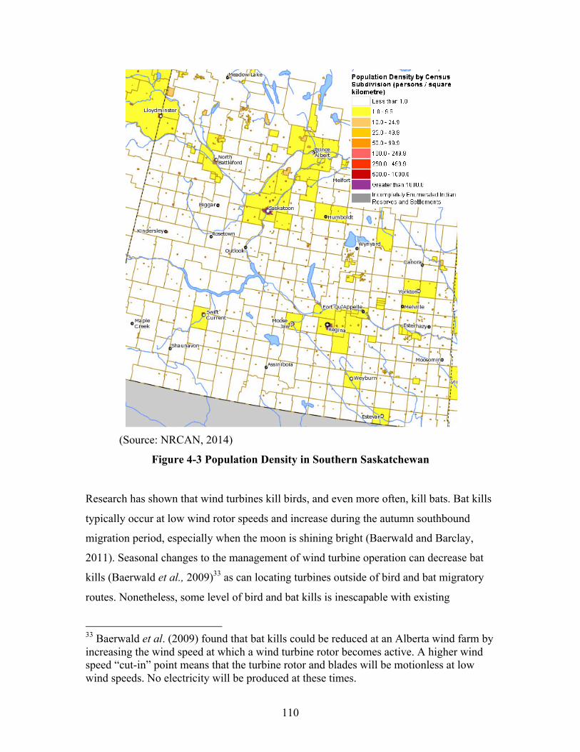
110

(Source: NRCAN, 2014)

Figure 4-3 Population Density in Southern Saskatchewan

Research has shown that wind turbines kill birds, and even more often, kill bats. Bat kills

typically occur at low wind rotor speeds and increase during the autumn southbound

migration period, especially when the moon is shining bright (Baerwald and Barclay,

2011). Seasonal changes to the management of wind turbine operation can decrease bat

kills (Baerwald et al., 2009)33 as can locating turbines outside of bird and bat migratory

routes. Nonetheless, some level of bird and bat kills is inescapable with existing

33 Baerwald et al. (2009) found that bat kills could be reduced at an Alberta wind farm by increasing the wind speed at which a wind turbine rotor becomes active. A higher wind speed “cut-in” point means that the turbine rotor and blades will be motionless at low wind speeds. No electricity will be produced at these times.

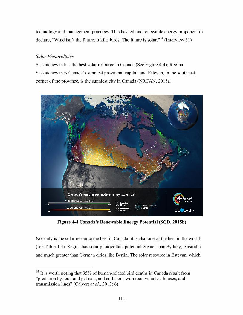
111

technology and management practices. This has led one renewable energy proponent to

declare, “Wind isn’t the future. It kills birds. The future is solar.”34 (Interview 31)

Solar Photovoltaics

Saskatchewan has the best solar resource in Canada (See Figure 4-4); Regina

Saskatchewan is Canada’s sunniest provincial capital, and Estevan, in the southeast

corner of the province, is the sunniest city in Canada (NRCAN, 2015a).

Figure 4-4 Canada’s Renewable Energy Potential (SCD, 2015b)

Not only is the solar resource the best in Canada, it is also one of the best in the world

(see Table 4-4). Regina has solar photovoltaic potential greater than Sydney, Australia

and much greater than German cities like Berlin. The solar resource in Estevan, which

34 It is worth noting that 95% of human-related bird deaths in Canada result from “predation by feral and pet cats, and collisions with road vehicles, houses, and transmission lines” (Calvert et al., 2013: 6).

112

achieves 1379 kwh/kw in a typical year, is nearly as high as the solar potential in Mexico

City (1425 kwh/kw). (NRCAN, 2015a). The greatest solar resource in Saskatchewan is

located in the southern half of the province, which happens to coincide with the majority

of the province’s population and electricity demand. Estevan also happens to be the

centre of Saskatchewan’s coal-fired power industry meaning that high-voltage

transmission lines connect the region to Regina and other load centres.

(Source: NRCAN, 2015a)

Table 4-4 Solar Photovoltaic in Cities Around the World

Despite the cold winters, the solar resource in Saskatchewan is present throughout the

course of the year (see Figure 4-5). Residents of the province will attest that, though the

winters are cold, the sun is often shining. The cold temperatures offer an additional boost

to solar potential in the province; the photovoltaic process is more efficient in colder

temperatures (Masters, 2004). As one participant remarked, the best place for solar is a

“cold desert” (Interview 28); Saskatchewan is just that. Saskatchewan’s northern location

does, however, mean that the days are shorter in the winter months and the solar potential

drops accordingly (Figure 4-5).

City

Yearly*PV*potential*(kWh/kW)

Cairo,'Egypt 1635Capetown,'South'Africa 1538New'Delhi,'India 1523Los'Angeles,'U.S.A 1485Mexico'City,'Mexico 1425Regina,*Saskatchewan 1361Sydney,'Australia 1343Rome,'Italy 1283Rio'de'Janeiro,'Brazil 1253Ottawa,'Canada 1198Beijing,'China 1148Washington,'D.C.,'U.S.A. 1133Paris,'France 938St.'John's,'Newfoundland/Labrador 933Tokyo,'Japan 885Berlin,'Germany 848Moscow,'Russia 803London,'England 728

113

Figure 4-5 Saskatchewan Solar Potential by Month in Four Select Cities

SaskPower does not currently own any utility-scale solar photovoltaic (PV) facilities.

Private homeowners and businesses have installed smaller residential and commercial

rooftop solar systems in the province, in part supported by the Ministry of Environment’s

Go Green fund. A comprehensive inventory of those projects is not currently available.

Biomass Potential

The majority of biomass potential in Saskatchewan lies along the boreal forest fringe.

The feedstock along the forest fringe consists of waste fibre leftover from pulp and paper

mills and sawmill operations. The Meadow Lake First Nation is currently developing a

biomass project using fuel from the latter. The project will be located beside the NorSask

sawmill in Meadow Lake and will offer roughly 36 MW of power (Interview 12). In

total, it is estimated that 120 MW of biomass potential exists along the forest fringe

(McKenzie quoted in Bigland-Pritchard and Prebble, 2010).

0

20

40

60

80

100

120

140

160

Janu

ary

Februa

ry

March

April

May

June

Ju

ly

Augus

t

Septem

ber

Octobe

r

Novem

ber

Decem

ber

Sol

ar P

hoto

volta

ic P

oten

tial (

kwh/

kw p

er m

onth

)

Month

Prince Albert Saskatoon Regina Estevan

114

Although burning the biomass does release carbon dioxide (CO2), these emissions are

treated as carbon neutral. This assumes that the trees will regrow where they have been

cut and uptake an equivalent amount of CO2 during their regrowth. As long as the forest

is continuously regrown the net addition of CO2 to the atmosphere will be zero.

Another biomass resource lies in the garbage dumps of the province. At a landfill,

organic matter rots in an anaerobic state and creates methane gas. The leaching of this

landfill methane gas is a measurable contributor to climate change. In 2013, 32

kilotonnes (kt) of methane (805 kt of carbon dioxide equivalent (CO2e)) was released due

to solid waste disposal on land in Saskatchewan; (Environment Canada, 2015a). Rather

than letting it leach to the atmosphere, the City of Saskatoon is using this landfill gas to

generate power. Tubes drilled into the landfill extract the methane, which is then burned

to generate electricity onsite. The Saskatoon plant has an electricity generating capacity

of 3.2 MW (CBC, 2012; City of Saskatoon, 2015). Proposals are now being made to

install solar photovoltaic panels at the landfill to supplement the electricity generated

using landfill gas (Interview 20).

Other smaller biomass projects can use crop residues from agriculture, manure from

intensive livestock operations, and landfill methane. It is assumed these smaller projects

could provide up to 30 MW of biomass power for a total of 150 MW of biomass potential

in the province.

Geothermal Potential

Deep geothermal heat has great potential for space heating and industrial processes in

Saskatchewan, but limited potential for direct electricity generation. Geothermal energy

for space heating was explored at the University of Regina (UofR) in the late 1970s. In

1978 a geothermal test hole was drilled at the UofR campus to a depth of 2226 meters.

Brought to the surface from this depth, the water has a temperature of 58-59°C. This hot

water was sufficient to meet a 2 MW heating load for a proposed sports complex. The

project was discontinued when plans for the sports complex fell through and oil prices

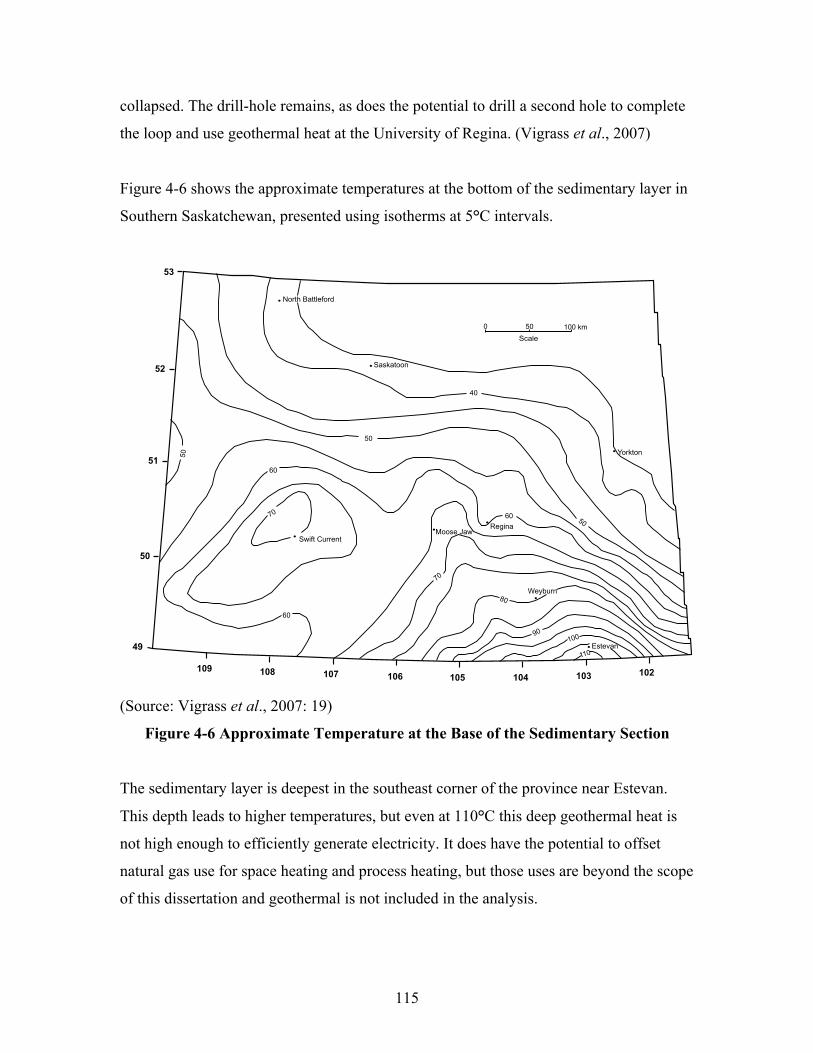
115

collapsed. The drill-hole remains, as does the potential to drill a second hole to complete

the loop and use geothermal heat at the University of Regina. (Vigrass et al., 2007)

Figure 4-6 shows the approximate temperatures at the bottom of the sedimentary layer in

Southern Saskatchewan, presented using isotherms at 5°C intervals.

(Source: Vigrass et al., 2007: 19)

Figure 4-6 Approximate Temperature at the Base of the Sedimentary Section

The sedimentary layer is deepest in the southeast corner of the province near Estevan.

This depth leads to higher temperatures, but even at 110°C this deep geothermal heat is

not high enough to efficiently generate electricity. It does have the potential to offset

natural gas use for space heating and process heating, but those uses are beyond the scope

of this dissertation and geothermal is not included in the analysis.

Saskatchewan Geological Survey 19 Summary of Investigations 2007, Volume 1

Figure 11 - Approximate temperature at the base of the sedimentary section in Saskatchewan south of latitude 53°N. Interval is 5°C.

reduced to 15.5°C (60°F). This would increase the heat extracted for both options (Table 11). In addition, a gas-fired or oil-fired boiler might be required to satisfy peak loads during the coldest weather and to serve as backup.

Heating industry representatives report that one million Btu/h are sufficient to meet the designed peak load of 45,000 ft2 (4181 m2) of energy-efficient commercial buildings. With heat pumps, Option One would provide heating for approximately 450,000 ft2 (41 810 m2) of commercial space and Option Two would heat about 735,000 ft2 (68 280 m2) of space, which, for district heating, would provide the peak heating load to at least 500 dwellings having average floor space of 1,470 ft2 (136.7 m2).

Table 11 - Primary circuit options for Regina area geothermal projects.

Estevan

Weyburn

Moose JawRegina

Swift Current

North Battleford

Saskatoon

Yorkton

40

50

60

70

60

70

80

90

110

60 50

50

Scale

0 100 km50

100

109 108 107 106 105 103 102104

49

50

51

52

53

Pumping Energy Surface Main Production Reda Injection Rate Production Exchanger Exchanger Casing Hole Casing Pump Pump Estimated

(usgpm) (Million Btu/h) Inlet Temp. Outlet Temp. Diameter Diameter Diameter Size Size Cost

Option One 264 6.7 58°C 30°C 273 mm 222 mm 178 mm 60 hp 20 hp $3,700,000(9.2)*

Option Two 458 12.0 59°C 30°C 340 mm 311 mm 244 mm 300 hp 100 hp $4,900,000(16.3)*

* Energy production in million Btu/h when heat pumps in secondary circuit are included. Estimated cost includes one vertical well, one directional (slant) hole, submersible pump, heat exchanger, and injection pump.

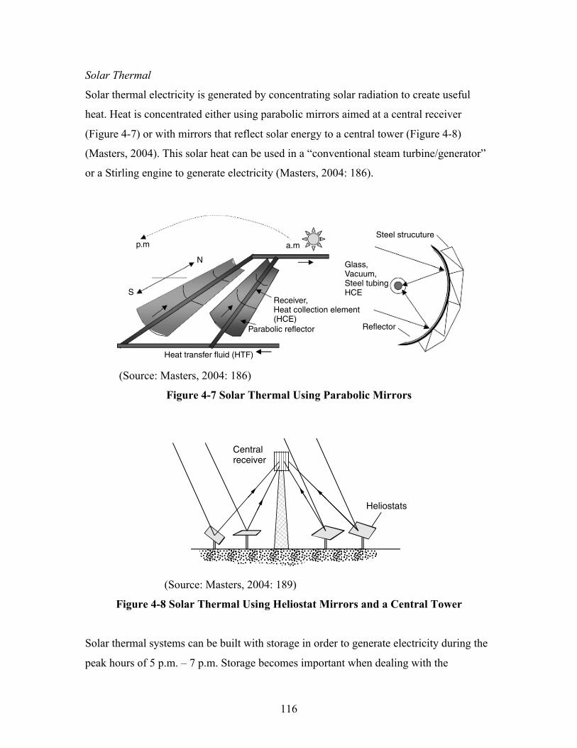
116

Solar Thermal

Solar thermal electricity is generated by concentrating solar radiation to create useful

heat. Heat is concentrated either using parabolic mirrors aimed at a central receiver

(Figure 4-7) or with mirrors that reflect solar energy to a central tower (Figure 4-8)

(Masters, 2004). This solar heat can be used in a “conventional steam turbine/generator”

or a Stirling engine to generate electricity (Masters, 2004: 186).

(Source: Masters, 2004: 186)

Figure 4-7 Solar Thermal Using Parabolic Mirrors

(Source: Masters, 2004: 189)

Figure 4-8 Solar Thermal Using Heliostat Mirrors and a Central Tower

Solar thermal systems can be built with storage in order to generate electricity during the

peak hours of 5 p.m. – 7 p.m. Storage becomes important when dealing with the

186 DISTRIBUTED GENERATION

TABLE 4.4 Second-Generation SAIC/STM Dish/Stirling SystemEfficienciesa

Step DescriptionStep

Efficiency (%)Cumulative

Efficiency (%)Power(kW)

Solar insolation 100.0 100 113.5Reflected by mirrors 93.1 93.1 105.7Intercepted at aperture 90.3 84.1 95.4Absorbed by receiver 85.0 71.5 81.1Receiver heat loss 98.0 70.0 79.5Engine mechanical efficiency 36.1 25.3 28.7Gear box efficiency 98.0 24.8 28.1Gross generator output 92.0 22.8 25.9Electrical parasites −2.2 kW 20.9 23.7

a Insolation is direct normal solar radiation at 1000 W/m2.Source: Davenport et al. (2002).

Electric Generation System (SEGS). SEGS consists of nine large arrays madeup of rows of parabolic-shaped mirrors that reflect and concentrate sunlight ontolinear receivers located along the foci of the parabolas. The receivers, or heatcollection elements (HCE), consist of a stainless steel absorber tube surroundedby a glass envelope with the vacuum drawn between the two to reduce heat losses.A heat transfer fluid circulates through the receivers, delivering the collectedsolar energy to a somewhat conventional steam turbine/generator to produceelectricity. The SEGS collectors, with over 2 million m2 of surface area, runalong a north–south axis, and they rotate from east to west to track the sunthroughout the day. Figure 4.9 illustrates the parabolic trough concept.

The first plant, SEGS I, is a 13.4-MW facility built in 1985, while thefinal plant, SEGS IX, produces 80 MW and was completed in 1991. SEGS I

p.m a.m

N

S

Glass,Vacuum,Steel tubingHCE

Steel strucuture

ReflectorParabolic reflector

Heat transfer fluid (HTF)

Receiver,Heat collection element(HCE)

Figure 4.9 Parabolic trough solar collector system.

CONCENTRATING SOLAR POWER (CSP) TECHNOLOGIES 189

4.3.3 Solar Central Receiver Systems

Another approach to achieving the concentrated sunlight needed for solar thermalpower plants is based on a system of computer-controlled mirrors, calledheliostats, which bounce sunlight onto a receiver mounted on top of a tower(Fig. 4.12).

The evolution of power towers began in 1976 with the establishment of theNational Solar Thermal Test Facility at Sandia National Laboratories in Albu-querque, New Mexico. That soon led to the construction of number of testfacilities around the world, the largest of which was a 90-m-tall, 10-MW powertower, called Solar One, built near Barstow, California. In Solar One, water waspumped up to the receiver where it was turned into steam that was brought backdown to a steam turbine/generator. Steam could also be diverted to a large, ther-mal storage tank filled with oil, rock, and sand to test the potential for continuedpower generation during marginal solar conditions or after the sun had set. Whilethermal storage as a concept was successfully demonstrated, there was a sizablemismatch between the storage tank temperature and the temperature needed bythe turbine for maximum efficiency.

Solar One operated from 1982 to 1988, after which time it was dismantled;parts of it, including the 1818 heliostats and the tower itself, were reused inanother 10-MW test facility called Solar Two. While Solar One used water asthe heat exchange medium, Solar Two used molten nitrate salts (60% sodiumnitrate and 40% potassium nitrate). A two-tank, molten-salt thermal storage sys-tem replaced the original oil/rock storage tank in the configuration shown inFig. 4.13. The molten-salt system has proven to be a great success. Its temper-ature of 565◦C well matches the needs of the steam turbine, and its round-tripefficiency (the ratio of thermal energy out to thermal energy in) was greater than97%. It was designed to provide enough storage to deliver the full 10-MW outputof the plant for an extra three hours past sunset. With reduced output, it coulddeliver power for much longer periods from stored solar energy.

Centralreceiver

Heliostats

Figure 4.12 Central receiver system (CRS) with heliostats to reflect sunlight onto acentral receiver.

117

variability of renewable energy (see discussion below). In a typical design, molten salt is

heated to 565°C and this heat can be used when desired to operate a steam turbine

(Masters, 2004).35

Southern Saskatchewan is one of the few places in Canada that receives enough sunshine

for solar thermal electricity to be generated. The total potential for solar thermal

electricity in Canada is estimated to be 26,190 TWh/yr on lands with slope less than 4%.

The Saskatchewan share of solar thermal potential is 13,575 TWh/yr; just over half of the

total. To put this in perspective total electricity generation in Saskatchewan in 2014 was

23.4 TWh (SaskPower, 2015). (Djebbar et al., 2014). However, for this total potential to

be achieved a good portion of southern Saskatchewan would be covered with solar

thermal reflective mirrors. The feasible potential is quite a bit smaller and is limited by

ability to access land, much of which is currently used for cereal production or

pastureland. The land requirements of the different technologies for solar thermal

electricity are as follows; “parabolic troughs about 5 acres/MW, and power towers about

8 acres/MW” (Masters, 2004: 191). On a typical section of land, measuring 1 mile by 1

mile or 640 acres, it would be possible to install 128 MW of parabolic trough solar

thermal or 80 MW using solar power towers.

Imported Hydroelectricity

A final renewable resource available to meet Saskatchewan electricity demand is

hydroelectricity imported from Manitoba, the province immediately to the east of

Saskatchewan. Manitoba’s electricity system is nearly 100% hydro-powered.36 The

utility, Manitoba Hydro, exports about 30% of the electricity they generate. The

Manitoba Hydro strategy has been to build hydro dams in the north of the province,

connect them with transmission lines through Winnipeg, in the southeast part of the

province, and export surplus power south to the United States. The sale of power to the

35 Storing heat to generate electricity is one of several methods of energy storage. I discuss storage further in Chapter 8. 36 In the fiscal year 2014-2015 Manitoba Hydro reported generated 35,000 Gigawatt-hours (GWh) using hydraulic generation out of a total of 35,044 GWh total generation (Manitoba Hydro, 2015a).

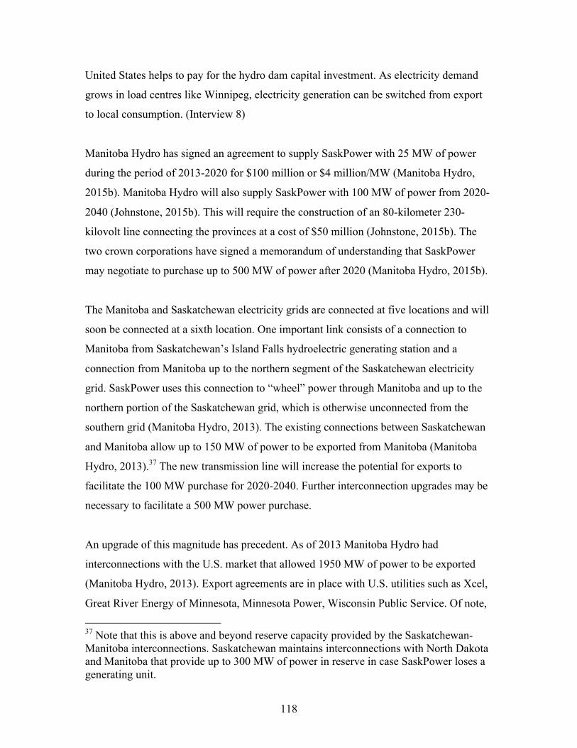
118

United States helps to pay for the hydro dam capital investment. As electricity demand

grows in load centres like Winnipeg, electricity generation can be switched from export

to local consumption. (Interview 8)

Manitoba Hydro has signed an agreement to supply SaskPower with 25 MW of power

during the period of 2013-2020 for $100 million or $4 million/MW (Manitoba Hydro,

2015b). Manitoba Hydro will also supply SaskPower with 100 MW of power from 2020-

2040 (Johnstone, 2015b). This will require the construction of an 80-kilometer 230-

kilovolt line connecting the provinces at a cost of $50 million (Johnstone, 2015b). The

two crown corporations have signed a memorandum of understanding that SaskPower

may negotiate to purchase up to 500 MW of power after 2020 (Manitoba Hydro, 2015b).

The Manitoba and Saskatchewan electricity grids are connected at five locations and will

soon be connected at a sixth location. One important link consists of a connection to

Manitoba from Saskatchewan’s Island Falls hydroelectric generating station and a

connection from Manitoba up to the northern segment of the Saskatchewan electricity

grid. SaskPower uses this connection to “wheel” power through Manitoba and up to the

northern portion of the Saskatchewan grid, which is otherwise unconnected from the

southern grid (Manitoba Hydro, 2013). The existing connections between Saskatchewan

and Manitoba allow up to 150 MW of power to be exported from Manitoba (Manitoba

Hydro, 2013).37 The new transmission line will increase the potential for exports to

facilitate the 100 MW purchase for 2020-2040. Further interconnection upgrades may be

necessary to facilitate a 500 MW power purchase.

An upgrade of this magnitude has precedent. As of 2013 Manitoba Hydro had

interconnections with the U.S. market that allowed 1950 MW of power to be exported

(Manitoba Hydro, 2013). Export agreements are in place with U.S. utilities such as Xcel,

Great River Energy of Minnesota, Minnesota Power, Wisconsin Public Service. Of note,

37 Note that this is above and beyond reserve capacity provided by the Saskatchewan-Manitoba interconnections. Saskatchewan maintains interconnections with North Dakota and Manitoba that provide up to 300 MW of power in reserve in case SaskPower loses a generating unit.

119

Xcel energy has nearly 6000 MW of wind power on their system. An export agreement to

purchase between 375 and 500 MW of hydropower from Manitoba helps to back-up

Xcel’s variable wind power resource. (Xcel, 2015; Manitoba Hydro, 2015b)

Summary of Potential

Saskatchewan has a strong wind resource and the best solar resource in Canada.

Additions of solar and wind capacity are limited by competing land uses, but the

available resources exceed Saskatchewan’s electricity needs by a large margin. The

province has 864 MW of hydroelectric capacity and the potential to develop an additional

1780 MW. Saskatchewan also has an opportunity to access significant hydroelectric

imports from neighbouring Manitoba. There is the potential for at least 150 MW of

biomass capacity to be built in the province, which would include biomass plants near

pulp and paper mills and sawmills, as well as landfill gas plants. Geothermal heat offers

the potential to substitute for space heating, but does not appear to offer significant

electricity generation potential. While the resource appears more than adequate for

Saskatchewan’s electricity needs, variability is a concern. I now turn to a discussion of

renewable energy variability in Saskatchewan.

120

Renewable Energy Variability

Renewable energy derived from wind and solar is fundamentally different from fossil

fuel derived energy. To use the language of system dynamics, wind and solar energy is

flow-limited, while fossil fuels are stock-limited. A flow-limited resource is one that is

limited by the flow of energy over time. A flow of blowing wind powers wind turbines. A

flow of solar insolation powers solar photovoltaics and solar thermal plants. Wind and

sunlight cannot be stored and saved for later; they must be used when available or else

they are wasted. They also cannot be used to generate power when they are not available;

wind turbines will not turn when the wind is not blowing and solar panels will not

generate electricity without light. (Daly and Farley, 2010)

Fossil fuels are stock-limited, but flow unlimited. The stock of coal in Saskatchewan’s

coal seams can be mined and burned in a power plant at a rate that lies within

SaskPower’s control (at the Poplar River station 12,000 tonnes of coal are strip-mined

and burned per day). These stocks of fossil fuels were built up over millennia; they are

the accumulation of the solar flow that collected in biomass and under heat and pressure

was transformed into fossil fuels. If we were to keep burning coal this stock would

eventually run out, or else become prohibitively expensive to extract. A stock of coal can

be saved for later. It can also be used up quickly if we so desire.

Hydropower and biomass exhibit elements of both flow-limited and stock-limited

resources. Hydropower is dependent on streamflow, which can vary year to year. In this

way it is flow-limited. The streamflow recharges hydro reservoirs, which can hold a stock

of water and release it on demand.

Biomass is fuelled by a flow of biomass growth and, if it is to be used sustainably, is

limited by the rate at which trees or crops grow. Biomass and biomass fuel can, however,

be accumulated in stocks. Forests can expand, and the stocks of biomass stored at

sawmills (e.g. along Saskatchewan’s forest fringe) can offer rich stores of biomass for

generating electricity.

121

Because renewables are flow-limited they are variable. They cannot be made available on

demand. This variability introduces challenges for electricity system operators. Wind and

solar cannot be turned on when load is required. Electricity operators must use other tools

to respond to this variability. For example, natural gas peaking plants are used to generate

power on short notice such as when there is a gap in renewable energy production.

Hydroelectric reservoirs can be used to store potential power and release it when needed.

Electricity can also be stored using technologies such as compressed air stored under

pressure in underground caverns; pumped hydro that moves water upstream or vertically

upwards in a mineshaft; fly-wheels; and lithium-ion batteries.

Below I outline the variability of electricity demand and renewables such as wind, solar,

and the stream flows that recharge hydroelectric reservoirs.

Wind Power Variability

Wind power varies with wind speed. Turbines do not begin to generate electricity until

winds reach a critical “cut-in” speed; for example Vestas V80 turbines begin to turn once

winds reach a speed of 4 meters/second (m/s) (Baerwald et al., 2009; Vestas, 2015).

Below the cut-in speed the output of a wind turbine is nil. Turbines also cut-out at high

wind speeds to prevent mechanical damage. For the Vestas V80 turbine, the rotors

disengage and stop turning when wind speeds reach 25 m/s (Vestas, 2015).

In 2013, SaskPower had 198 MW of wind power on their system. The average power

output of the wind turbines was 72.7 MW, creating a capacity factor of 36.7% over the

course of the year. The power output of the wind turbines could swing significantly from

hour to hour. The largest swings were a ramp up of 119.1 MW from 20:00 to 21:00 on

January 18th and a ramp down of 118 MW between the hours of 9:00 and 10:00 on

January 18th, 2013. This large swing would have required other power generation

facilities to ramp down from 20:00 to 21:00 and ramp up between 9:00 and 10:00 in order

to balance the changes in wind power production. Figure 4-9 shows the 24-hour period

with the highest wind power variance in 2013. Wind power ramped up from zero to near

full capacity and then back down again over the course of January 29th.

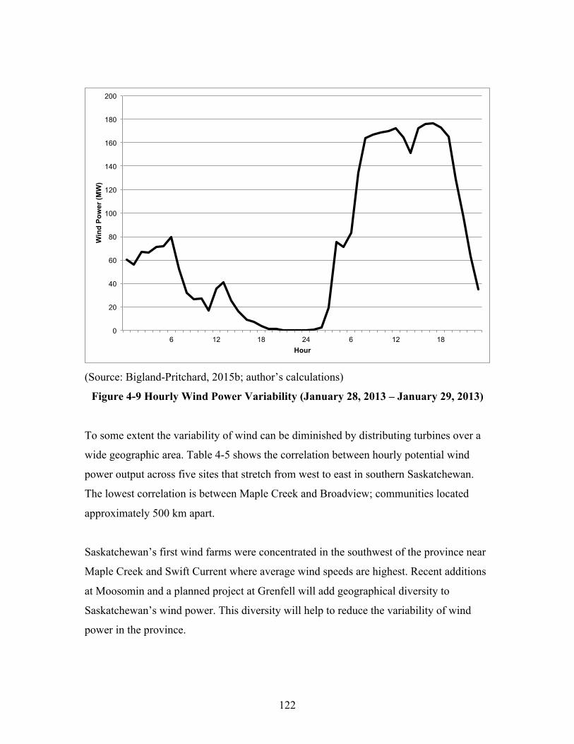
122

(Source: Bigland-Pritchard, 2015b; author’s calculations)

Figure 4-9 Hourly Wind Power Variability (January 28, 2013 – January 29, 2013)

To some extent the variability of wind can be diminished by distributing turbines over a

wide geographic area. Table 4-5 shows the correlation between hourly potential wind

power output across five sites that stretch from west to east in southern Saskatchewan.

The lowest correlation is between Maple Creek and Broadview; communities located

approximately 500 km apart.

Saskatchewan’s first wind farms were concentrated in the southwest of the province near

Maple Creek and Swift Current where average wind speeds are highest. Recent additions

at Moosomin and a planned project at Grenfell will add geographical diversity to

Saskatchewan’s wind power. This diversity will help to reduce the variability of wind

power in the province.

0

20

40

60

80

100

120

140

160

180

200

6 12 18 24 6 12 18

Win

d Po

wer

(MW

)

Hour

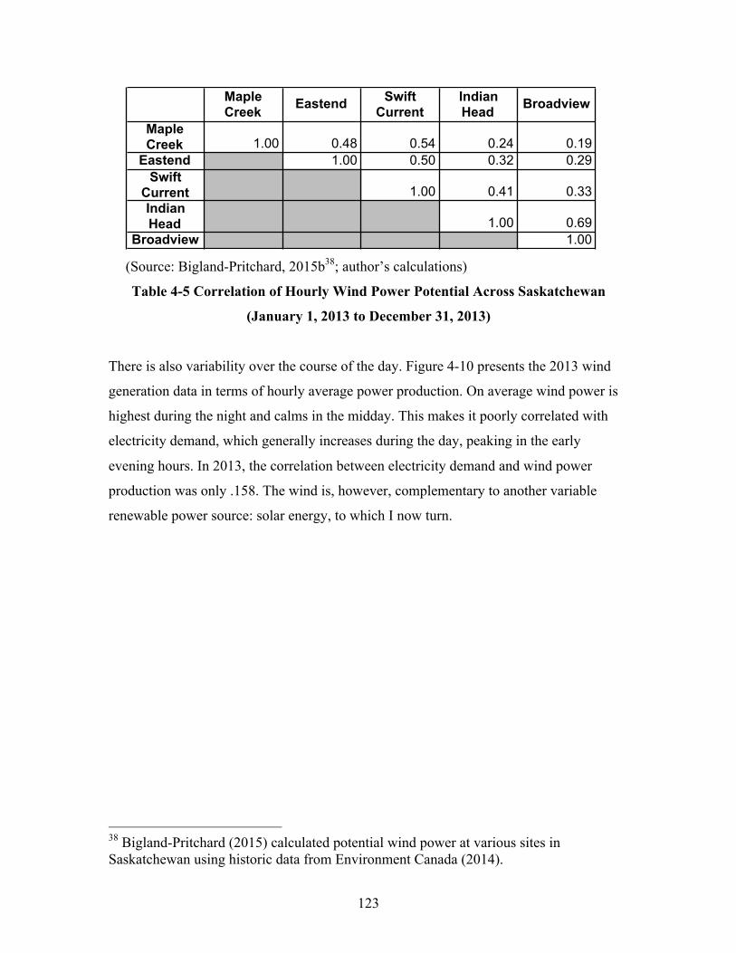
123

(Source: Bigland-Pritchard, 2015b38; author’s calculations)

Table 4-5 Correlation of Hourly Wind Power Potential Across Saskatchewan

(January 1, 2013 to December 31, 2013)

There is also variability over the course of the day. Figure 4-10 presents the 2013 wind

generation data in terms of hourly average power production. On average wind power is

highest during the night and calms in the midday. This makes it poorly correlated with

electricity demand, which generally increases during the day, peaking in the early

evening hours. In 2013, the correlation between electricity demand and wind power

production was only .158. The wind is, however, complementary to another variable

renewable power source: solar energy, to which I now turn.

38 Bigland-Pritchard (2015) calculated potential wind power at various sites in Saskatchewan using historic data from Environment Canada (2014).

Maple Creek Eastend Swift

CurrentIndian Head Broadview

Maple Creek 1.00 0.48 0.54 0.24 0.19

Eastend 1.00 0.50 0.32 0.29Swift

Current 1.00 0.41 0.33Indian Head 1.00 0.69

Broadview 1.00

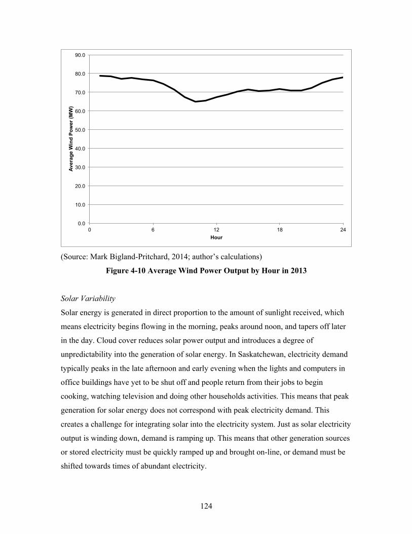
124

(Source: Mark Bigland-Pritchard, 2014; author’s calculations)

Figure 4-10 Average Wind Power Output by Hour in 2013

Solar Variability

Solar energy is generated in direct proportion to the amount of sunlight received, which

means electricity begins flowing in the morning, peaks around noon, and tapers off later

in the day. Cloud cover reduces solar power output and introduces a degree of

unpredictability into the generation of solar energy. In Saskatchewan, electricity demand

typically peaks in the late afternoon and early evening when the lights and computers in

office buildings have yet to be shut off and people return from their jobs to begin

cooking, watching television and doing other households activities. This means that peak

generation for solar energy does not correspond with peak electricity demand. This

creates a challenge for integrating solar into the electricity system. Just as solar electricity

output is winding down, demand is ramping up. This means that other generation sources

or stored electricity must be quickly ramped up and brought on-line, or demand must be

shifted towards times of abundant electricity.

0.0

10.0

20.0

30.0

40.0

50.0

60.0

70.0

80.0

90.0

0 6 12 18 24

Ave

rage

Win

d Po

wer

(MW

)

Hour

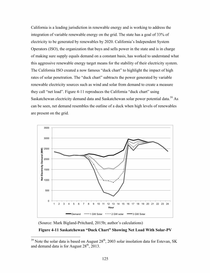
125

California is a leading jurisdiction in renewable energy and is working to address the

integration of variable renewable energy on the grid. The state has a goal of 33% of

electricity to be generated by renewables by 2020. California’s Independent System

Operators (ISO), the organization that buys and sells power in the state and is in charge

of making sure supply equals demand on a constant basis, has worked to understand what

this aggressive renewable energy target means for the stability of their electricity system.

The California ISO created a now famous “duck chart” to highlight the impact of high

rates of solar penetration. The “duck chart” subtracts the power generated by variable

renewable electricity sources such as wind and solar from demand to create a measure

they call “net load”. Figure 4-11 reproduces the California “duck chart” using

Saskatchewan electricity demand data and Saskatchewan solar power potential data.39 As

can be seen, net demand resembles the outline of a duck when high levels of renewables

are present on the grid.

(Source: Mark Bigland-Pritchard, 2015b; author’s calculations)

Figure 4-11 Saskatchewan “Duck Chart” Showing Net Load With Solar-PV 39 Note the solar data is based on August 28th, 2003 solar insolation data for Estevan, SK and demand data is for August 28th, 2013.

0

500

1000

1500

2000

2500

3000

3500

1 2 3 4 5 6 7 8 9 10 11 12 13 14 15 16 17 18 19 20 21 22 23 24

Net

Ele

ctric

ity D

eman

d (M

W)

Hour

Demand 1 GW Solar 2 GW solar 3 GW Solar

126

If Saskatchewan were to invest heavily in solar photovoltaics (solar-PV) plans would

have to be made to ensure smooth integration into the system. On the afternoon depicted

in Figure 4-11, the ramp-up of a significant source of non-solar electricity would be

required. For example, in the scenario with 3 GW of installed solar power, net demand

(demand minus solar output) increases by 1900 MW between 1:00 and 4:00 p.m. This

means that 1900 MW of capacity must be brought online during that period. Although

this is an extreme example – this day was selected because it had the largest ramp-up

requirement of all possible days in the dataset – the electricity system must be able to

respond to even the most extreme cases in order to reliably supply Saskatchewan’s

electricity needs.

Proponents of solar point out that the electricity system is built to follow the variability of

electricity demand; response to variability is already built into the electricity system

(Lazar, 2014). Lazar (2014) notes that “ducks vary their shape depending on different

circumstances…utility load shapes can do the same” (Lazar, 2014: 2). He outlines ten

strategies that can minimize the difference between demand and net load and “teach the

duck to fly” (Lazar, 2014):

1. Target energy efficiency to periods when net load ramps most quickly; this could

mean encouraging LED lighting to reduce residential lighting demand in the

evening;

2. Orient solar panels to the west to generate more power in the late afternoon,

which may be worthwhile even if total power output declines;

3. Build some solar thermal with storage to shift the availability of solar power

towards the peak demand hours of late afternoon and early evening;

4. Allow grid operator to manage electric water heating loads: electric water heaters

can be superheated during times of plentiful electricity generation and blended

with cool water when needed in the supper hours;

5. Build air conditioners with thermal storage; this is less important in

Saskatchewan, but would include storing cold by creating ice during the middle of

the night;

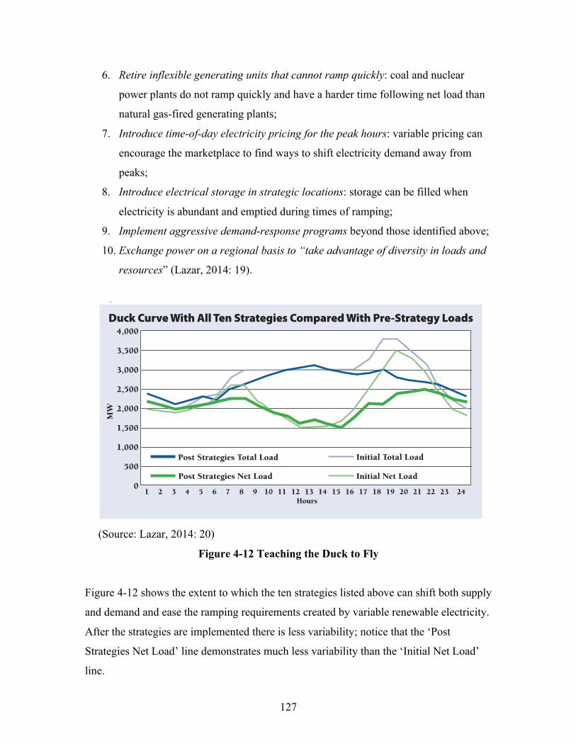
127

6. Retire inflexible generating units that cannot ramp quickly: coal and nuclear

power plants do not ramp quickly and have a harder time following net load than

natural gas-fired generating plants;

7. Introduce time-of-day electricity pricing for the peak hours: variable pricing can

encourage the marketplace to find ways to shift electricity demand away from

peaks;

8. Introduce electrical storage in strategic locations: storage can be filled when

electricity is abundant and emptied during times of ramping;

9. Implement aggressive demand-response programs beyond those identified above;

10. Exchange power on a regional basis to “take advantage of diversity in loads and

resources” (Lazar, 2014: 19).

(Source: Lazar, 2014: 20)

Figure 4-12 Teaching the Duck to Fly

Figure 4-12 shows the extent to which the ten strategies listed above can shift both supply

and demand and ease the ramping requirements created by variable renewable electricity.

After the strategies are implemented there is less variability; notice that the ‘Post

Strategies Net Load’ line demonstrates much less variability than the ‘Initial Net Load’

line.

Teaching the “Duck” To Fly

20

It is useful now to compare our final result – with all ten strategies – to the starting point with acquisition of renewable resources, but without the strategies. Figure 16 shows the end result compared with the starting point.

Figure 17 Airborne Ducks

Our newly streamlined duck needs only to stretch his wings, try a few beats, and see if he can become airborne like his cousins.

Figure 16

Duck Curve With All Ten Strategies Compared With Pre-Strategy Loads

Post Strategies Total Load

Post Strategies Net Load

Initial Total Load

Initial Net Load

Hours

MW

1 2 3 4 5 6 7 8 9 10 11 12 13 14 15 16 17 18 19 20 21 22 23 24

4,000

3,500

3,000

2,500

2,000

1,500

1,000

500

0

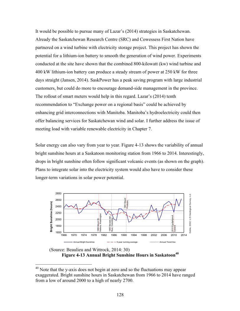
128

It would be possible to pursue many of Lazar’s (2014) strategies in Saskatchewan.

Already the Saskatchewan Research Centre (SRC) and Cowessess First Nation have

partnered on a wind turbine with electricity storage project. This project has shown the

potential for a lithium-ion battery to smooth the generation of wind power. Experiments

conducted at the site have shown that the combined 800-kilowatt (kw) wind turbine and

400 kW lithium-ion battery can produce a steady stream of power at 250 kW for three

days straight (Jansen, 2014). SaskPower has a peak saving program with large industrial

customers, but could do more to encourage demand-side management in the province.

The rollout of smart meters would help in this regard. Lazar’s (2014) tenth

recommendation to “Exchange power on a regional basis” could be achieved by

enhancing grid interconnections with Manitoba. Manitoba’s hydroelectricity could then

offer balancing services for Saskatchewan wind and solar. I further address the issue of

meeting load with variable renewable electricity in Chapter 7.

Solar energy can also vary from year to year. Figure 4-13 shows the variability of annual

bright sunshine hours at a Saskatoon monitoring station from 1966 to 2014. Interestingly,

drops in bright sunshine often follow significant volcanic events (as shown on the graph).

Plans to integrate solar into the electricity system would also have to consider these

longer-term variations in solar power potential.

(Source: Beaulieu and Wittrock, 2014: 30)

Figure 4-13 Annual Bright Sunshine Hours in Saskatoon40

40 Note that the y-axis does not begin at zero and so the fluctuations may appear exaggerated. Bright sunshine hours in Saskatchewan from 1966 to 2014 have ranged from a low of around 2000 to a high of nearly 2700.

SRC Publication No. 10440-1E14

SRC Climate Reference Station Annual Summary, 2013 February 2014

page 30

RADIATION G

oble

, 200

2; U

.S G

eolo

gica

l Sur

vey,

n.d

.

Annual bright Sunshine Hours

Seasonal bright Sunshine Hours

Monthly bright Sunshine Hours

Monthly Comparison bright Sunshine Hours, Global & Diffuse Radiation

1650

1850

2050

2250

2450

2650

2850

1966 1970 1974 1978 1982 1986 1990 1994 1998 2002 2006 2010 2014

brig

ht S

unsh

ine

(hou

rs)

Annual Bright Sunshine 5-year running average Annual Trend line

1980

Mou

nt S

t. H

elen

s, W

ashi

ngto

n

1991

Mou

nt

Pina

tubo

,

1985

Nev

ado

del

Rui

z, C

olom

bia

2010

Eyj

ufja

lljok

ull,

Icel

and

0

200

400

600

800

1000

1200

1966 1970 1974 1978 1982 1986 1990 1994 1998 2002 2006 2010 2014

brig

ht S

unsh

ine

(hou

rs)

Winter Total DJF Spring Total MAM Summer Total JJA Autumn Total SONWinter Trend line Spring Trend line Summer Trend line Autumn Trend line

0

500

1000

1500

2000

2500

3000

0

100

200

300

400

500

600

Jan Feb Mar Apr May June July Aug Sep Oct Nov Dec Cum

ulat

ive

brig

ht S

unsh

ine

(h

ours

)

brig

ht S

unsh

ine

(hou

rs)

2013 Bright Sunshine (hours) Normal Bright Sunshine (hours)Possible Bright Sunshine* (hours) 2013 Cumulative Bright Sunshine (hours)Normal Cumulative Bright Sunshine (hours)

0

60

120

180

240

300

360

420

0

100

200

300

400

500

600

700

Jan Feb Mar Apr May June July Aug Sep Oct Nov Dec

brig

ht S

unsh

ine

(hou

rs)

Rad

iatio

n (M

j/m

2 )

2013 Global Radiation (MJ/m2) 2013 Diffuse Radiation (MJ/m2) Normal Diffuse Radiation (MJ/m2)Normal Global Radiation (MJ/m2) 2013 Bright Sunshine (hours) Normal Bright Sunshine (hours)

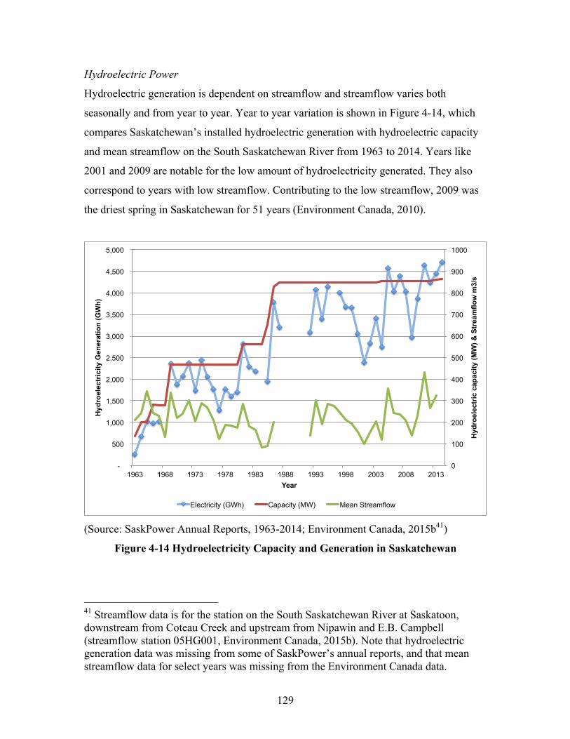
129

Hydroelectric Power

Hydroelectric generation is dependent on streamflow and streamflow varies both

seasonally and from year to year. Year to year variation is shown in Figure 4-14, which

compares Saskatchewan’s installed hydroelectric generation with hydroelectric capacity

and mean streamflow on the South Saskatchewan River from 1963 to 2014. Years like

2001 and 2009 are notable for the low amount of hydroelectricity generated. They also

correspond to years with low streamflow. Contributing to the low streamflow, 2009 was

the driest spring in Saskatchewan for 51 years (Environment Canada, 2010).

(Source: SaskPower Annual Reports, 1963-2014; Environment Canada, 2015b41)

Figure 4-14 Hydroelectricity Capacity and Generation in Saskatchewan

41 Streamflow data is for the station on the South Saskatchewan River at Saskatoon, downstream from Coteau Creek and upstream from Nipawin and E.B. Campbell (streamflow station 05HG001, Environment Canada, 2015b). Note that hydroelectric generation data was missing from some of SaskPower’s annual reports, and that mean streamflow data for select years was missing from the Environment Canada data.

0

100

200

300

400

500

600

700

800

900

1000

-

500

1,000

1,500

2,000

2,500

3,000

3,500

4,000

4,500

5,000

1963 1968 1973 1978 1983 1988 1993 1998 2003 2008 2013 H

ydro

elec

tric

cap

acity

(MW

) & S

trea

mflo

w m

3/s

Hyd

roel

ectr

icity

Gen

erat

ion

(GW

h)

Year

Electricity (GWh) Capacity (MW) Mean Streamflow

130

When hydroelectricity is a large part of an electricity system, planners must be aware of

the potential for drought. The Saskatchewan River system, home to 84% of current

hydroelectric capacity in the province, depends on snowmelt and rainfall runoff from the

Rocky Mountains (Sauchyn et al., 2011). The long-run historic record shows that “mega-

droughts” of up to 30 years have occurred in the Saskatchewan system; one in the early

1700s and another in the mid 1100s (Sauchyn et al., 2011). The Saskatchewan River

system is fed by snowmelt from the Rocky Mountains. If climate change lowers snowfall

in the Rockies then Saskatchewan’s hydroelectric potential will suffer. However, even

without impacts from anthropogenic climate change, long-lasting drought is a possibility

on the prairies and could reduce hydroelectric output in the future.42

Streamflow in Saskatchewan is highly seasonal, peaking in June due to the accumulated

effects of spring runoff. Hydroelectric production closely follows this seasonal pattern,

although hydroelectric reservoirs such as Diefenbaker Lake and Tobin Lake allow

streamflow to be stored for release later in time and can smooth hydroelectric production

to a certain extent. (See Figure 4-15).

Figure 4-15 shows hydroelectricity generation in Saskatchewan from 2009-2013 (solid

black line) along with streamflow on both the South Saskatchewan River, measured at

Saskatoon (dashed blue line), and the North Saskatchewan River, measured at Prince

Albert (solid light green line).43 The station at Saskatoon is downstream from Coteau

Creek and upstream from Nipawin and E.B. Campbell. Flows at the Saskatoon station are

influenced by decisions made regarding hydroelectric production at Coteau Creek. The

Saskatoon station shows summer peak flows, but also increased flows in the winter

months. This coincides with the highest electricity demand in Saskatchewan; it is a

winter-peaking province. The North Saskatchewan River at Prince Albert, which has no

42 System planners in Manitoba have accounted for the variability of river systems in that province by building more hydroelectric capacity than is needed for provincial use and making conservative estimates of reliable streamflow. Yet even these conservative estimates do not account for the potential of multi-decadal mega-drought. 43 The Prince Albert station is streamflow station 05GG001 (Environment Canada, 2015b).

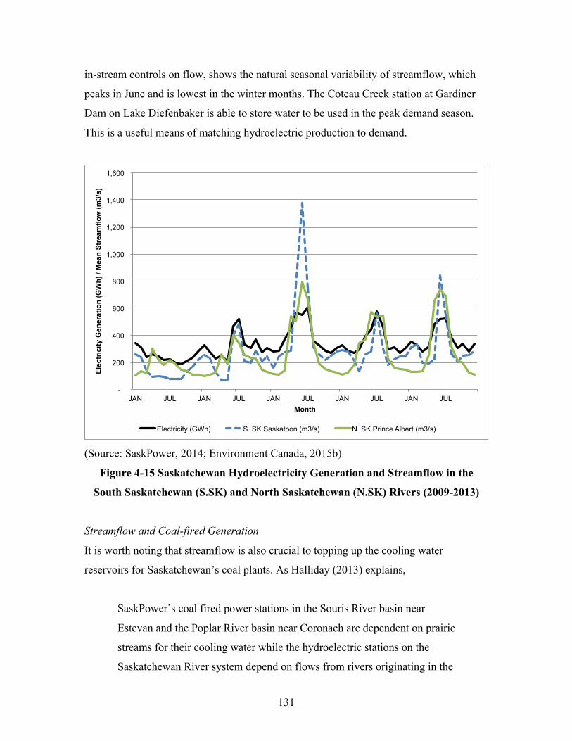
131

in-stream controls on flow, shows the natural seasonal variability of streamflow, which

peaks in June and is lowest in the winter months. The Coteau Creek station at Gardiner

Dam on Lake Diefenbaker is able to store water to be used in the peak demand season.

This is a useful means of matching hydroelectric production to demand.

(Source: SaskPower, 2014; Environment Canada, 2015b)

Figure 4-15 Saskatchewan Hydroelectricity Generation and Streamflow in the

South Saskatchewan (S.SK) and North Saskatchewan (N.SK) Rivers (2009-2013)

Streamflow and Coal-fired Generation

It is worth noting that streamflow is also crucial to topping up the cooling water

reservoirs for Saskatchewan’s coal plants. As Halliday (2013) explains,

SaskPower’s coal fired power stations in the Souris River basin near

Estevan and the Poplar River basin near Coronach are dependent on prairie

streams for their cooling water while the hydroelectric stations on the

Saskatchewan River system depend on flows from rivers originating in the

-

200

400

600

800

1,000

1,200

1,400

1,600

JAN JUL JAN JUL JAN JUL JAN JUL JAN JUL

Ele

ctri

city

Gen

erat

ion

(GW

h) /

Mea

n S

trea

mflo

w (m

3/s)

Month

Electricity (GWh) S. SK Saskatoon (m3/s) N. SK Prince Albert (m3/s)

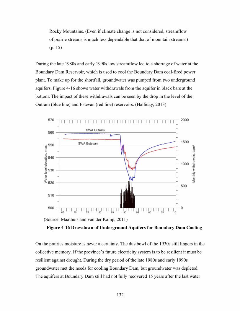
132

Rocky Mountains. (Even if climate change is not considered, streamflow

of prairie streams is much less dependable that that of mountain streams.)

(p. 15)

During the late 1980s and early 1990s low streamflow led to a shortage of water at the

Boundary Dam Reservoir, which is used to cool the Boundary Dam coal-fired power

plant. To make up for the shortfall, groundwater was pumped from two underground

aquifers. Figure 4-16 shows water withdrawals from the aquifer in black bars at the

bottom. The impact of these withdrawals can be seen by the drop in the level of the

Outram (blue line) and Estevan (red line) reservoirs. (Halliday, 2013)

(Source: Maathuis and van der Kamp, 2011)

Figure 4-16 Drawdown of Underground Aquifers for Boundary Dam Cooling

On the prairies moisture is never a certainty. The dustbowl of the 1930s still lingers in the

collective memory. If the province’s future electricity system is to be resilient it must be

resilient against drought. During the dry period of the late 1980s and early 1990s

groundwater met the needs for cooling Boundary Dam, but groundwater was depleted.

The aquifers at Boundary Dam still had not fully recovered 15 years after the last water

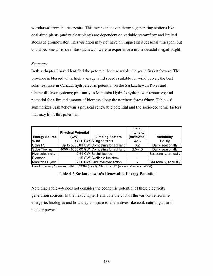
133

withdrawal from the reservoirs. This means that even thermal generating stations like

coal-fired plants (and nuclear plants) are dependent on variable streamflow and limited

stocks of groundwater. This variation may not have an impact on a seasonal timespan, but

could become an issue if Saskatchewan were to experience a multi-decadal megadrought.

Summary

In this chapter I have identified the potential for renewable energy in Saskatchewan. The

province is blessed with: high average wind speeds suitable for wind power; the best

solar resource in Canada; hydroelectric potential on the Saskatchewan River and

Churchill River systems; proximity to Manitoba Hydro’s hydropower resources; and

potential for a limited amount of biomass along the northern forest fringe. Table 4-6

summarizes Saskatchewan’s physical renewable potential and the socio-economic factors

that may limit this potential.

Table 4-6 Saskatchewan’s Renewable Energy Potential

Note that Table 4-6 does not consider the economic potential of these electricity

generation sources. In the next chapter I evaluate the cost of the various renewable

energy technologies and how they compare to alternatives like coal, natural gas, and

nuclear power.

Energy SourcePhysical Potential

(GW) Limiting Factors

Land Intensity

(ha/MWac) VariabilityWind >4.00 GW Siting conflicts 42.3 HourlySolar PV Up to 5300.00 GW Competing for agl land 3.2 Daily, seasonallySolar Thermal 4000 - 8000.00 GW Competing for agl land 2.0-4.0 Daily, seasonallyHydroelectricity 2.64 GW Social license - Seasonally, annuallyBiomass .15 GW Available fuelstock -Manitoba Hydro 2.00 GW Grid interconnection - Seasonally, annuallyLand Intensity Sources: NREL, 2009 (wind); NREL, 2013 (solar); Masters (2004)

134

Chapter 5 – Levelized Cost of Electricity Generation

Electricity Generation Technologies

SaskPower is making decisions on how to meet Saskatchewan electricity demand by

considering a range of generation technologies. In this chapter I explore the cost of

building new capacity and generating electricity in Saskatchewan using the following

technologies:

• Biomass;

• Conventional coal-fired generation;

• Coal-fired generation with carbon-capture and storage (CCS);

• Hydroelectric new-build;

• Hydroelectric repower (retrofit);

• Natural gas combined cycle;

• Natural gas combined cycle with CCS;

• Natural gas simple cycle (peaking plants);

• Small, modular nuclear reactors;

• Solar photovoltaic (utility-scale);

• Solar thermal (utility-scale);

• Wind turbines.

I am also interested in the cost of adding electricity storage to the Saskatchewan grid.

Storage can be a useful way of addressing the variability of renewable energy output and,

depending on the circumstances, should be included in the cost of renewables. Several

technologies exist that could provide electricity storage in Saskatchewan including:

lithium-ion batteries, compressed air storage, and pumped hydro storage. Compressed air

storage may be particularly well-suited for Saskatchewan. It requires an underground

cavern to store the compressed air. This cavern could be a former natural gas storage

cavern or a solution-mined salt dome (Ford, 2015). Saskatchewan is home to both of

these resources. I explore the question of storage further in Chapter 7.

135

There are several costs associated with installing and operating the electricity generation

technologies listed above. These include the capital cost of building the technology, the

cost of operating and maintaining the technology, fuel costs for coal, natural gas,

biomass, and nuclear technologies, as well as technology-specific costs such as water

usage charges for hydroelectricity, land leases for wind turbines, and nuclear waste

storage costs for nuclear power plants. There are also financing costs associated with

borrowing funds to purchase the technologies. In this chapter I outline the assumptions I

have made with respect to each of these costs. These cost assumptions are used as inputs

to the Saskatchewan Investment Model (SIM) and the interactive Saskatchewan

Investment Model (iSIM) and play a key role in determining the least-cost scenarios

selected by the SIM and iSIM optimization models.

Levelized Cost of Electricity

When comparing the costs of electricity generation technologies it is necessary to

consider the operating characteristics of each technology. Electricity generation

technologies differ with regards to capacity factors, expected life span, and fuel

efficiency.44 These differences in operating characteristics mean that technologies

generate different quantities of electricity with the same installed capacity. For example,

a 100 MW solar installation that operates at a 14-20% capacity factor will generate less

electricity annually than a 100 MW coal-fired plant operating at 75-85% capacity factor.

The Levelized Cost of Electricity (LCOE) takes these differences into consideration.

LCOE is a measure of the average cost of electricity generation for a given technology

44 EPRI (2013) explains capacity factor in the following way, “The maximum number of megawatt-hours that a plant could produce in one year would occur if the plant operated at full load 24 hours a day for 365 days a year. In reality, a plant will be shut down at times during the year, either for maintenance or because the electricity is not needed and it would be uneconomical to operate the plant” (EPRI, 2013: 24/1-7). The capacity factor of coal-fired and nuclear plants that are run fairly continuously throughout the year may be as high as 85-90%. Variable renewable electricity technologies like wind turbines do not operate in a continuous manner; electricity generation depends on the presence of wind. The capacity factor for Saskatchewan’s wind turbines in 2014 was 36.5% (SaskPower, 2015; author’s calculations). The life span of various electricity generation technologies also differs: wind turbines have a lifespan of about 20 years; hydroelectric facilities are relatively long-lived at 40 years or longer. For more information on fuel efficiency please see the technical appendix at the end of this chapter.

136

over its lifetime. It is expressed in either dollars per megawatt-hour ($/MWh) or cents per

kilowatt-hour (cents/kWh) and it is the standard measure for comparing the costs of

electricity generation technologies.45

Several recent studies have used the LCOE measure. Citigroup’s Global Perspectives &

Solutions (Citi GPS, 2015) published a report entitled Energy Darwinism II that used

LCOE to compare the cost of climate action to the cost of climate inaction. Because

LCOE includes fuel costs Citi GPS (2015) was able to demonstrate that renewables,

despite their high capital costs, are rapidly becoming cost competitive with fossil fuel

generation. Because of this Citi GPS (2015) found that climate action would actually save

money relative to a path of climate inaction. Coad (2015) used LCOE numbers as the

basis of a Conference Board study that included a focused look at the Saskatchewan

electricity sector. Coad (2015) calculated the portfolio of electricity generation

technologies that would minimize investor risk in the province. Lazard (2014) published

the eighth edition of their levelized cost comparison in Fall 2014. It is widely cited in the

electricity literature. The Global CCS Institute (2015) used LCOE to compare low-carbon

technologies to the cost of CCS. They found that renewable technologies like wind,

geothermal, and hydroelectricity, when available, provide lower cost GHG reductions

than CCS. Figure 5-1 presents the range of LCOE values that result from the various cost

assumptions presented in the literature. All figures have been converted to 2014 Canadian

dollars (2014 $CAN) using the all-items consumer price index (Statistics Canada, 2015

CANSIM Table 326-0020) and average annual US-CAN exchange rates (Bank of

Canada, 2015).

45 As a long-term average LCOE does have the drawback of not considering the market value of electricity. Market prices can vary throughout the course of the day. Some technologies, like solar-PV may coincide with high demand and high demand in certain seasons. Others, like wind, may provide power during times when prices are low. LCOE misses these aspects of the value of electricity. Studies such as Dewees (2012) take into consideration the cost of electricity displaced by variable renewables.

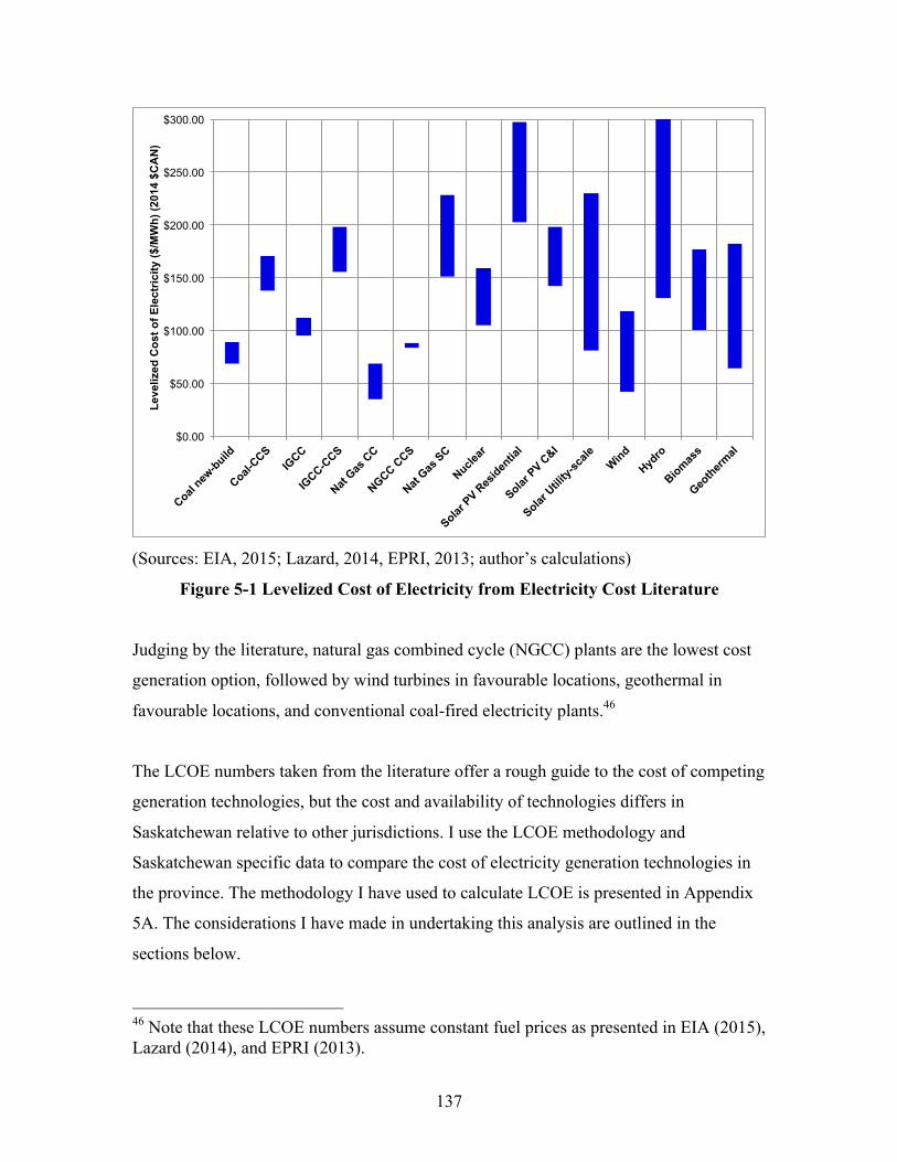
137

(Sources: EIA, 2015; Lazard, 2014, EPRI, 2013; author’s calculations)

Figure 5-1 Levelized Cost of Electricity from Electricity Cost Literature

Judging by the literature, natural gas combined cycle (NGCC) plants are the lowest cost

generation option, followed by wind turbines in favourable locations, geothermal in

favourable locations, and conventional coal-fired electricity plants.46

The LCOE numbers taken from the literature offer a rough guide to the cost of competing

generation technologies, but the cost and availability of technologies differs in

Saskatchewan relative to other jurisdictions. I use the LCOE methodology and

Saskatchewan specific data to compare the cost of electricity generation technologies in

the province. The methodology I have used to calculate LCOE is presented in Appendix

5A. The considerations I have made in undertaking this analysis are outlined in the

sections below.

46 Note that these LCOE numbers assume constant fuel prices as presented in EIA (2015), Lazard (2014), and EPRI (2013).

$0.00

$50.00

$100.00

$150.00

$200.00

$250.00

$300.00

Coal new

-build

Coal-CCS

IGCC

IGCC-C

CS

Nat Gas

CC

NGCC CCS

Nat Gas

SC

Nuclear

Solar PV R

esiden

tial

Solar PV C

&I

Solar U

tility-

scale

Wind

Hydro

Biomass

Geotherm

al

Leve

lized

Cos

t of E

lect

ricity

($/M

Wh)

(201

4 $C

AN

)

138

Saskatchewan Capital Costs

I gathered capital costs from published figures of projects built in Saskatchewan. When

Saskatchewan project costs are not available I use cost input assumptions found in

publications such as EIA (2015), Lazard (2014), and EPRI (2013). I find a range of

capital costs for various energy generation technologies (Figure 5-2). The blue diamonds

in Figure 5-2 indicate capital costs in dollars per kilowatt ($/kw) for SaskPower projects,

or in the case of nuclear, for the most recent quote on nuclear power obtained in Canada.

In the context of the present research the following findings are of particular interest.

First, the cost of coal with carbon capture and storage (CCS) is significantly higher than

estimates from the literature. Saskatchewan’s Boundary Dam III CCS project is the first

utility-scale CCS project in the world. The project was originally budgeted to cost $1.24

billion, but costs have increased to $1.46 billion (CAN) (IEAGHG, 2015). Costs were

higher than expected due to factors such as a shortage of skilled workers in the province,

which increased wages paid to labour, and challenges with retrofitting a brownfield

power plant site (IEAGHG, 2015).

A second insight that should be highlighted is that there is a premium paid for thermal

construction in Saskatchewan. Capital costs for natural gas combined cycle plants built in

Saskatchewan, including the North Battleford Generating Station and the retrofit to the

Queen Elizabeth II power plant in Saskatoon, are approximately 2.6 times higher than

EIA (2015). Costs for simple cycle natural gas plants are on average 1.8 times higher

than EIA (2015). To account for this premium I apply a cost multiplier of 2.0 to EIA

(2015) estimates of natural gas combined cycle with CCS costs. This may be an

optimistic multiplier for an un-tested technology like natural gas with CCS.

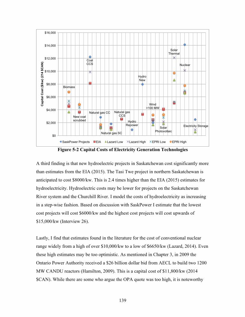
139

Figure 5-2 Capital Costs of Electricity Generation Technologies

A third finding is that new hydroelectric projects in Saskatchewan cost significantly more

than estimates from the EIA (2015). The Tasi Twe project in northern Saskatchewan is

anticipated to cost $8000/kw. This is 2.4 times higher than the EIA (2015) estimates for

hydroelectricity. Hydroelectric costs may be lower for projects on the Saskatchewan

River system and the Churchill River. I model the costs of hydroelectricity as increasing

in a step-wise fashion. Based on discussion with SaskPower I estimate that the lowest

cost projects will cost $6000/kw and the highest cost projects will cost upwards of

$15,000/kw (Interview 26).

Lastly, I find that estimates found in the literature for the cost of conventional nuclear

range widely from a high of over $10,000/kw to a low of $6650/kw (Lazard, 2014). Even

these high estimates may be too optimistic. As mentioned in Chapter 3, in 2009 the

Ontario Power Authority received a $26 billion dollar bid from AECL to build two 1200

MW CANDU reactors (Hamilton, 2009). This is a capital cost of $11,800/kw (2014

$CAN). While there are some who argue the OPA quote was too high, it is noteworthy

Coal CCS

Natural gas CC

Hydro Repower

Hydro New

Wind >100 MW

Natural gas CCS

Electricity Storage

Biomass

New coal scrubbed

Natural gas SC

Solar Photovoltaic

Solar Thermal

Nuclear

$0

$2,000

$4,000

$6,000

$8,000

$10,000

$12,000

$14,000

$16,000

Cap

ital C

ost (

$/kw

) (21

4 $C

AN

)

SaskPower Projects EIA Lazard Low Lazard High EPRI Low EPRI High

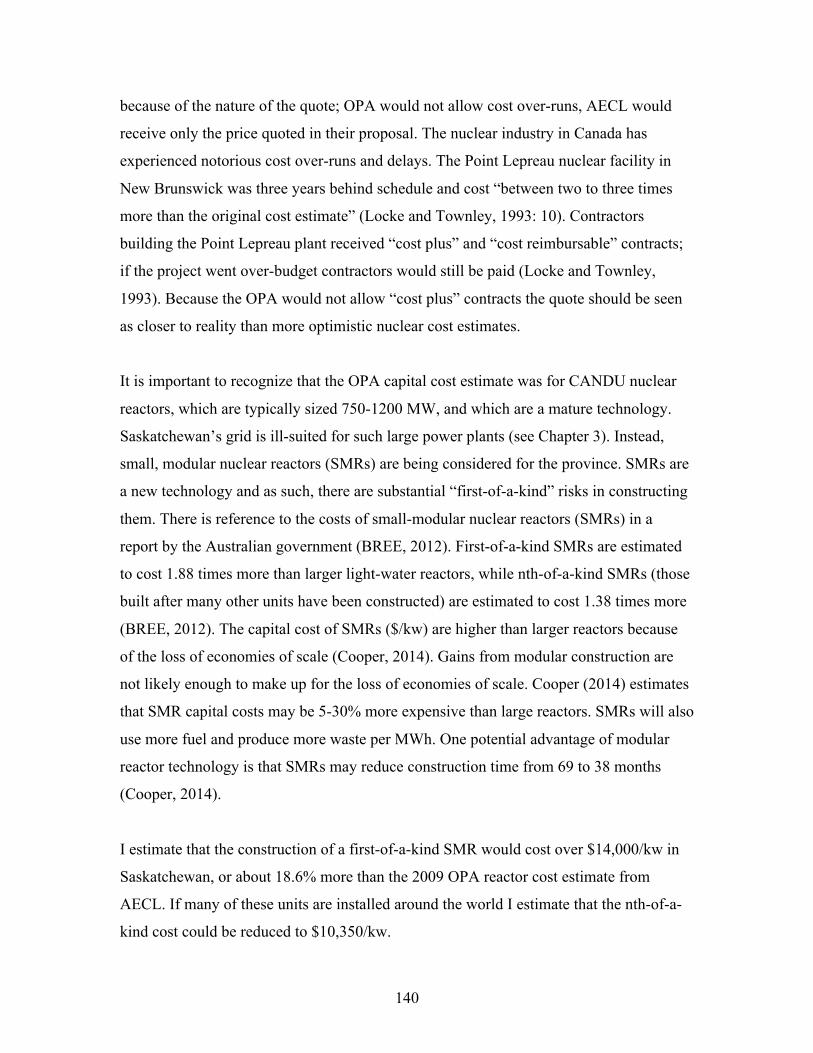
140

because of the nature of the quote; OPA would not allow cost over-runs, AECL would

receive only the price quoted in their proposal. The nuclear industry in Canada has

experienced notorious cost over-runs and delays. The Point Lepreau nuclear facility in

New Brunswick was three years behind schedule and cost “between two to three times

more than the original cost estimate” (Locke and Townley, 1993: 10). Contractors

building the Point Lepreau plant received “cost plus” and “cost reimbursable” contracts;

if the project went over-budget contractors would still be paid (Locke and Townley,

1993). Because the OPA would not allow “cost plus” contracts the quote should be seen

as closer to reality than more optimistic nuclear cost estimates.

It is important to recognize that the OPA capital cost estimate was for CANDU nuclear

reactors, which are typically sized 750-1200 MW, and which are a mature technology.

Saskatchewan’s grid is ill-suited for such large power plants (see Chapter 3). Instead,

small, modular nuclear reactors (SMRs) are being considered for the province. SMRs are

a new technology and as such, there are substantial “first-of-a-kind” risks in constructing

them. There is reference to the costs of small-modular nuclear reactors (SMRs) in a

report by the Australian government (BREE, 2012). First-of-a-kind SMRs are estimated

to cost 1.88 times more than larger light-water reactors, while nth-of-a-kind SMRs (those

built after many other units have been constructed) are estimated to cost 1.38 times more

(BREE, 2012). The capital cost of SMRs ($/kw) are higher than larger reactors because

of the loss of economies of scale (Cooper, 2014). Gains from modular construction are

not likely enough to make up for the loss of economies of scale. Cooper (2014) estimates

that SMR capital costs may be 5-30% more expensive than large reactors. SMRs will also

use more fuel and produce more waste per MWh. One potential advantage of modular

reactor technology is that SMRs may reduce construction time from 69 to 38 months

(Cooper, 2014).

I estimate that the construction of a first-of-a-kind SMR would cost over $14,000/kw in

Saskatchewan, or about 18.6% more than the 2009 OPA reactor cost estimate from

AECL. If many of these units are installed around the world I estimate that the nth-of-a-

kind cost could be reduced to $10,350/kw.

141

Sensitivity to Carbon Pricing

The LCOE of a fossil-fuel technology will be affected by the imposition of carbon

pricing. I find that technologies that use coal and natural gas as fuels are quite sensitive to

carbon pricing. In Saskatchewan, coal fired power plants emit roughly 1080 tonnes

CO2e/MWh. When equipped with carbon capture and storage (CCS) technology, 90% of

these emissions can be captured. However, there is a substantial parasitic load involved in

capturing CO2. At the Boundary Dam III CCS facility a 160 Megawatt (MW) generation

unit is rated at 120 MW available power. The other 40 MW are required to run the CCS

processes. This means the emissions intensity of coal-fired generation with CCS is not

10% of the intensity of coal-fired generation without CCS but is actually 143 tonnes

CO2e/MWh, which is 13.2% of the existing GHG intensity.

Natural gas combined cycle facilities in Saskatchewan have an emissions intensity of

approximately 420 tonnes CO2e/MWh. If natural gas combined cycle plants are equipped

with a CCS system then 90% of their emissions can be captured and stored. There is

again parasitic power demand to run the CCS process. I estimate that natural gas with

CCS will lead to a 20% penalty in fuel efficiency. With this parasitic load considered,

natural gas with CCS can reduce emissions intensity to approximately 50 tonnes

CO2e/MWh.

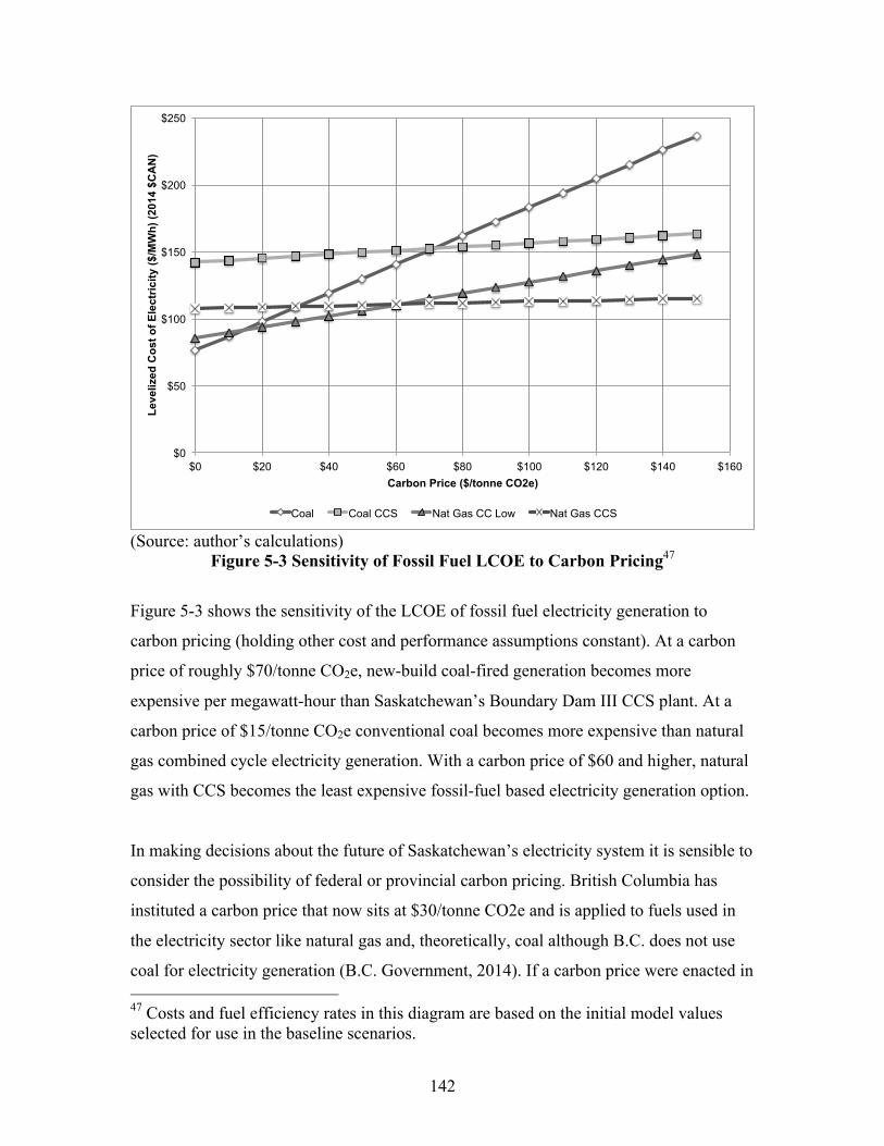
142

(Source: author’s calculations)

Figure 5-3 Sensitivity of Fossil Fuel LCOE to Carbon Pricing47

Figure 5-3 shows the sensitivity of the LCOE of fossil fuel electricity generation to

carbon pricing (holding other cost and performance assumptions constant). At a carbon

price of roughly $70/tonne CO2e, new-build coal-fired generation becomes more

expensive per megawatt-hour than Saskatchewan’s Boundary Dam III CCS plant. At a

carbon price of $15/tonne CO2e conventional coal becomes more expensive than natural

gas combined cycle electricity generation. With a carbon price of $60 and higher, natural

gas with CCS becomes the least expensive fossil-fuel based electricity generation option.

In making decisions about the future of Saskatchewan’s electricity system it is sensible to

consider the possibility of federal or provincial carbon pricing. British Columbia has

instituted a carbon price that now sits at $30/tonne CO2e and is applied to fuels used in

the electricity sector like natural gas and, theoretically, coal although B.C. does not use

coal for electricity generation (B.C. Government, 2014). If a carbon price were enacted in 47 Costs and fuel efficiency rates in this diagram are based on the initial model values selected for use in the baseline scenarios.

$0

$50

$100

$150

$200

$250

$0 $20 $40 $60 $80 $100 $120 $140 $160

Leve

lized

Cos

t of E

lect

ricity

($/M

Wh)

(201

4 $C

AN

)

Carbon Price ($/tonne CO2e)

Coal Coal CCS Nat Gas CC Low Nat Gas CCS

143

Saskatchewan natural gas with CCS would be roughly cost-equivalent to new-build coal-

fired generation.

Fuel Cost Escalation and LCOE

Along with carbon price risks there are also fuel price risks that can influence the

levelized cost of electricity (LCOE).48 Natural gas is an especially volatile commodity. In

the past decade, natural gas delivered at The Henry Hub has varied in price from highs of

$13.42 USD/Million BTU in October 2005 and $12.69 USD/MMBTU to a low of

$1.95/MMBTU in April of 2012 (See Figure 5-4).49 The Henry Hub price for August

2015 remained low at $2.77 USD/MMBTU.

(Source: EIA, 2015)

Figure 5-4 Natural Gas Price at Louisiana’s Henry Hub

48 Appendix 5A outlines the method I use to calculate fuel use for fossil fuel technologies. 49 Henry Hub is a natural gas distribution hub in Louisiana. Natural gas prices at the Henry Hub are regularly used as a benchmark for natural gas pricing.

0

2

4

6

8

10

12

14

16

Jan-

1997

Jan-

1998

Jan-

1999

Jan-

2000

Jan-

2001

Jan-

2002

Jan-

2003

Jan-

2004

Jan-

2005

Jan-

2006

Jan-

2007

Jan-

2008

Jan-

2009

Jan-

2010

Jan-

2011

Jan-

2012

Jan-

2013

Jan-

2014

Jan-

2015

Dol

lars

per

Mill

ion

Btu

(US

D)

Henry Hub Natural Gas Spot Price (Dollars per Million Btu)

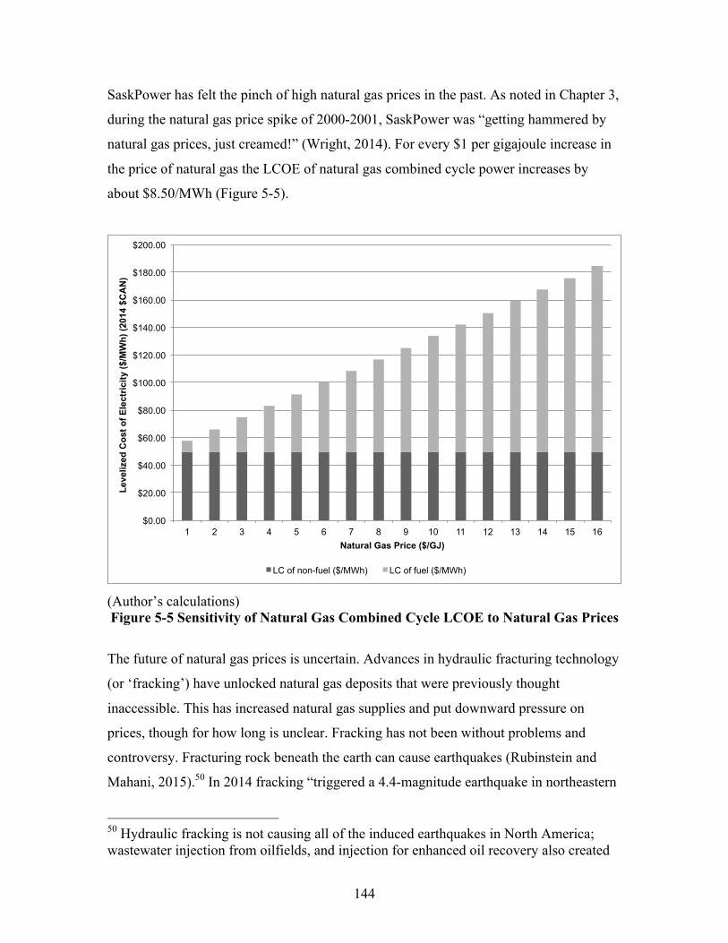
144

SaskPower has felt the pinch of high natural gas prices in the past. As noted in Chapter 3,

during the natural gas price spike of 2000-2001, SaskPower was “getting hammered by

natural gas prices, just creamed!” (Wright, 2014). For every $1 per gigajoule increase in

the price of natural gas the LCOE of natural gas combined cycle power increases by

about $8.50/MWh (Figure 5-5).

(Author’s calculations) Figure 5-5 Sensitivity of Natural Gas Combined Cycle LCOE to Natural Gas Prices

The future of natural gas prices is uncertain. Advances in hydraulic fracturing technology

(or ‘fracking’) have unlocked natural gas deposits that were previously thought

inaccessible. This has increased natural gas supplies and put downward pressure on

prices, though for how long is unclear. Fracking has not been without problems and

controversy. Fracturing rock beneath the earth can cause earthquakes (Rubinstein and

Mahani, 2015).50 In 2014 fracking “triggered a 4.4-magnitude earthquake in northeastern

50 Hydraulic fracking is not causing all of the induced earthquakes in North America; wastewater injection from oilfields, and injection for enhanced oil recovery also created

$0.00

$20.00

$40.00

$60.00

$80.00

$100.00

$120.00

$140.00

$160.00

$180.00

$200.00

1 2 3 4 5 6 7 8 9 10 11 12 13 14 15 16

Leve

lized

Cos

t of E

lect

rici

ty ($

/MW

h) (2

014

$CA

N)

Natural Gas Price ($/GJ)

LC of non-fuel ($/MWh) LC of fuel ($/MWh)

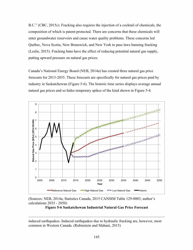
145

B.C.” (CBC, 2015c). Fracking also requires the injection of a cocktail of chemicals, the

composition of which is patent-protected. There are concerns that these chemicals will

enter groundwater reservoirs and cause water quality problems. These concerns led

Québec, Nova Scotia, New Brunswick, and New York to pass laws banning fracking

(Leslie, 2015). Fracking bans have the effect of reducing potential natural gas supply,

putting upward pressure on natural gas prices.

Canada’s National Energy Board (NEB, 2014a) has created three natural gas price

forecasts for 2013-2035. These forecasts are specifically for natural gas prices paid by

industry in Saskatchewan (Figure 5-6). The historic time series displays average annual

natural gas prices and so hides temporary spikes of the kind shown in Figure 5-4.

(Sources: NEB, 2014a; Statistics Canada, 2015 CANSIM Table 129-0003; author’s calculations 2035 - 2050)

Figure 5-6 Saskatchewan Industrial Natural Gas Price Forecast

induced earthquakes. Induced earthquakes due to hydraulic fracking are, however, most common in Western Canada. (Rubinstein and Mahani, 2015)

0

1

2

3

4

5

6

7

8

9

2000 2005 2010 2015 2020 2025 2030 2035 2040 2045 2050

Nat

ural

Gas

Pric

e ($

/GJ)

(201

4 $C

AN

)

Year

Reference Natural Gas High Natural Gas Low Natural Gas Historic

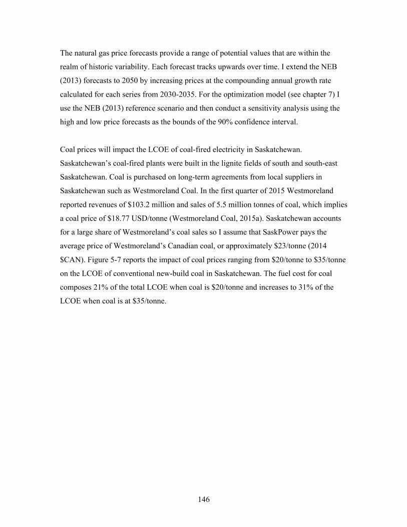
146

The natural gas price forecasts provide a range of potential values that are within the

realm of historic variability. Each forecast tracks upwards over time. I extend the NEB

(2013) forecasts to 2050 by increasing prices at the compounding annual growth rate

calculated for each series from 2030-2035. For the optimization model (see chapter 7) I

use the NEB (2013) reference scenario and then conduct a sensitivity analysis using the

high and low price forecasts as the bounds of the 90% confidence interval.

Coal prices will impact the LCOE of coal-fired electricity in Saskatchewan.

Saskatchewan’s coal-fired plants were built in the lignite fields of south and south-east

Saskatchewan. Coal is purchased on long-term agreements from local suppliers in

Saskatchewan such as Westmoreland Coal. In the first quarter of 2015 Westmoreland

reported revenues of $103.2 million and sales of 5.5 million tonnes of coal, which implies

a coal price of $18.77 USD/tonne (Westmoreland Coal, 2015a). Saskatchewan accounts

for a large share of Westmoreland’s coal sales so I assume that SaskPower pays the

average price of Westmoreland’s Canadian coal, or approximately $23/tonne (2014

$CAN). Figure 5-7 reports the impact of coal prices ranging from $20/tonne to $35/tonne

on the LCOE of conventional new-build coal in Saskatchewan. The fuel cost for coal

composes 21% of the total LCOE when coal is $20/tonne and increases to 31% of the

LCOE when coal is at $35/tonne.

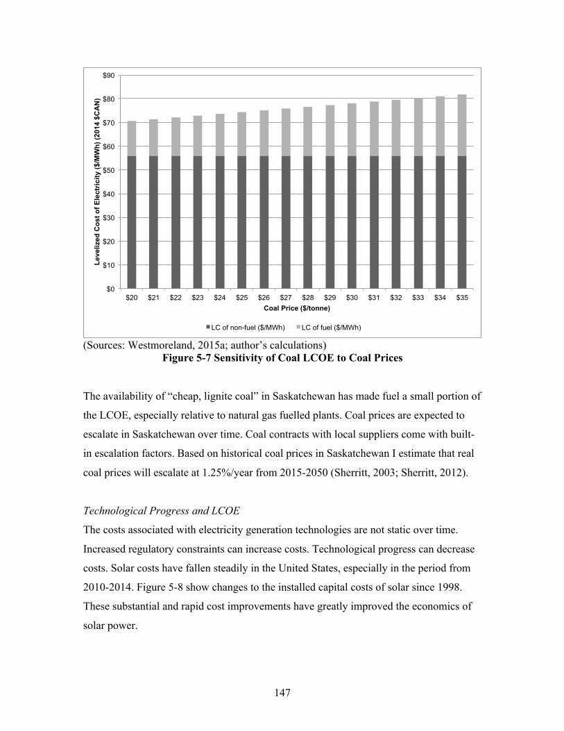
147

(Sources: Westmoreland, 2015a; author’s calculations)

Figure 5-7 Sensitivity of Coal LCOE to Coal Prices

The availability of “cheap, lignite coal” in Saskatchewan has made fuel a small portion of

the LCOE, especially relative to natural gas fuelled plants. Coal prices are expected to

escalate in Saskatchewan over time. Coal contracts with local suppliers come with built-

in escalation factors. Based on historical coal prices in Saskatchewan I estimate that real

coal prices will escalate at 1.25%/year from 2015-2050 (Sherritt, 2003; Sherritt, 2012).

Technological Progress and LCOE

The costs associated with electricity generation technologies are not static over time.

Increased regulatory constraints can increase costs. Technological progress can decrease

costs. Solar costs have fallen steadily in the United States, especially in the period from

2010-2014. Figure 5-8 show changes to the installed capital costs of solar since 1998.

These substantial and rapid cost improvements have greatly improved the economics of

solar power.

$0

$10

$20

$30

$40

$50

$60

$70

$80

$90

$20 $21 $22 $23 $24 $25 $26 $27 $28 $29 $30 $31 $32 $33 $34 $35

Leve

lized

Cos

t of E

lect

rici

ty ($

/MW

h) (2

014

$CA

N)

Coal Price ($/tonne)

LC of non-fuel ($/MWh) LC of fuel ($/MWh)

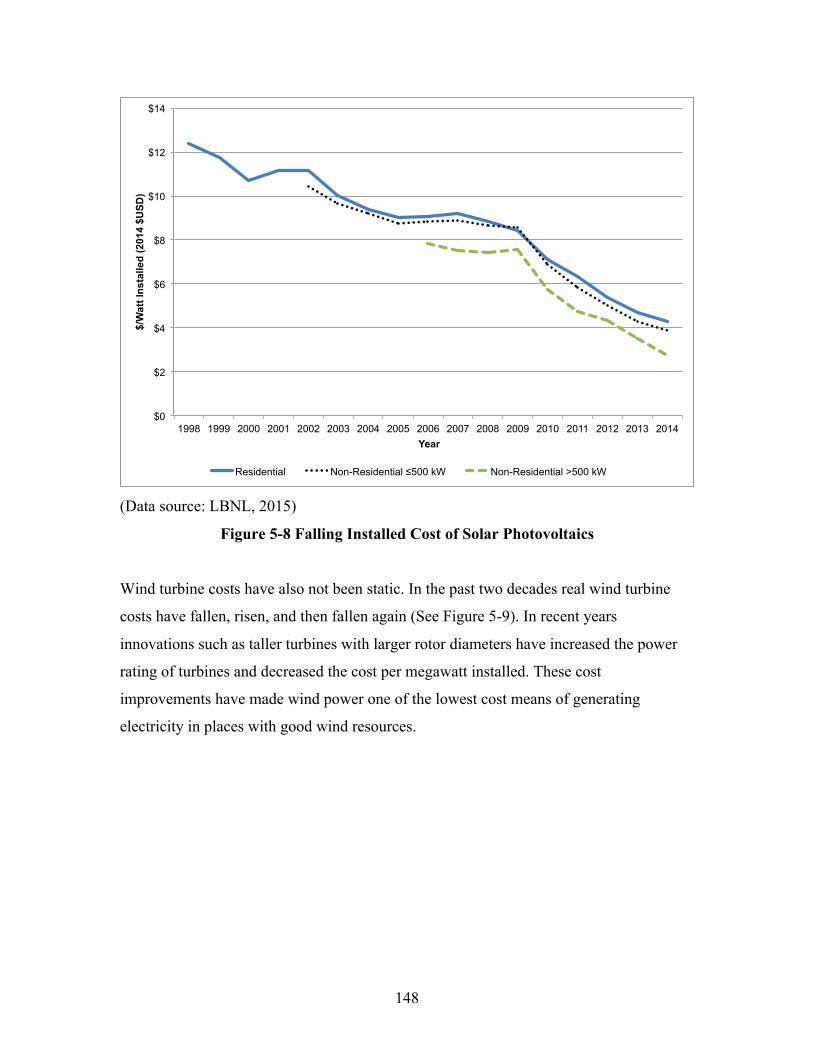
148

(Data source: LBNL, 2015)

Figure 5-8 Falling Installed Cost of Solar Photovoltaics

Wind turbine costs have also not been static. In the past two decades real wind turbine

costs have fallen, risen, and then fallen again (See Figure 5-9). In recent years

innovations such as taller turbines with larger rotor diameters have increased the power

rating of turbines and decreased the cost per megawatt installed. These cost

improvements have made wind power one of the lowest cost means of generating

electricity in places with good wind resources.

$0

$2

$4

$6

$8

$10

$12

$14

1998 1999 2000 2001 2002 2003 2004 2005 2006 2007 2008 2009 2010 2011 2012 2013 2014

$/W

att I

nsta

lled

(201

4 $U

SD)

Year

Residential Non-Residential ≤500 kW Non-Residential >500 kW

149

(Source: U.S. DoE, 2015: 47)

Figure 5-9 Wind Power Transaction Prices in the United States (1997-2015)

The rate at which costs change is called the “learning rate”. Learning can be modeled as

an exogenous force acting upon costs, or as an endogenous outcome of “learning-by-

doing” (Löschel, 2002). From a “learning-by-doing” perspective, costs change as

experience is built up installing a technology. For example, Citi GPS (2015) comments

on learning rates that have occurred with a doubling of installed capacity,

Solar in particular was exhibiting learning rates in excess of 20% (i.e.

the cost of a panel would fall by >20% for every doubling of installed

capacity), wind at 7.4%, gas was evolving via the shale revolution in

the US, while nuclear was becoming more expensive, and liquefied

natural gas (LNG) had also increased in cost... (Citi GPS, 2015: 46)

Endogenous learning-by-doing models are useful when analyzing changes to costs in

large economies like the United States whose market size is large enough to generate

learning-by-doing effects. At just under 5000 Megawatts (MW), the province of

Saskatchewan has a relatively small electricity system. Saskatchewan purchases of

2014 Wind Technologies Market Report 47

Source: Berkeley Lab

Figure 38. Reported wind turbine transaction prices over time

Since 2008, wind turbine prices have declined substantially, reflecting a reversal of some of the previously mentioned underlying trends that had earlier pushed prices higher as well as increased competition among manufacturers and significant cost-cutting measures on the part of turbine and component suppliers. As shown in Figure 38, our limited sample of recently announced U.S. turbine transactions shows pricing in the $850–$1,250/kW range. Bloomberg NEF (2015b) reports global average pricing for recent contracts of $950-1,200/kW. Data from Vestas largely confirm these pricing points, with average global prices dropping to roughly $1,175/kW in 2014.

Overall, these figures suggest price declines of 20%–40% since late 2008. Moreover, these declines have been coupled with improved turbine technology (e.g., the recent growth in average hub heights and rotor diameters shown in Chapter 4) and more-favorable terms for turbine purchasers (e.g., reduced turbine delivery lead times and less need for large frame-agreement orders, longer initial O&M contract durations, improved warranty terms, and more-stringent performance guarantees). These price reductions and improved terms have exerted downward pressure on total project costs and wind power prices, whereas increased rotor diameters and hub heights are improving capacity factors and further reducing wind power prices.

Lower turbine prices have driven reductions in reported installed project costs

Berkeley Lab compiles data on the total installed cost of wind power projects in the United States, including data on 36 projects completed in 2014 totaling 3,888 MW, or 80% of the wind power capacity installed in that year. In aggregate, the dataset (through 2014) includes 743 completed wind power projects in the continental United States totaling 54,014 MW and equaling roughly 82% of all wind power capacity installed in the United States at the end of 2014. In general, reported project costs reflect turbine purchase and installation, balance of plant, and any substation and/or interconnection expenses. Data sources are diverse, however, and are

150

electricity generation technology are too small to induce noticeable learning-by-doing

effects. For this reason I treat learning as something that happens outside of

Saskatchewan and I treat learning rates in Saskatchewan as exogenous cost improvements

per year. Citi GPS (2015) translates learning rates for wind and solar into the following

annual averages, “For solar PV modules the year on year reduction would amount to 2%

whilst for onshore wind this number is 1%” (p. 47).

Coad (2015) uses a simple exogenous learning rate equation to model changes to

technology costs over time,

𝐸𝑞. 5.1 𝐶𝑜𝑠𝑡! = 𝐶𝑜𝑠𝑡! ∗ 𝑒𝑥𝑝!!"

Where,

𝛾 = learning rate

𝑡 = time.

I also use Equation 5.1 to represent learning. This type of equation can be used to

calculate or apply average annual learning rates.

I calculate learning rates for each technology using data from EIA (2014). This report

presents levelized cost of capital, variable O&M, and fixed O&M costs for 2019 and

2040. I use Equation 5.1 to estimate the learning rate implied by the cost changes in EIA

(2014). These learning rates are summarized in Table 5.1. EIA (2014) is optimistic that

capital costs for nuclear will fall by 1.54%/yr. Estimates for the annual capital cost

improvement of solar are 1.25%, a figure lower than the current rate of cost

improvement.

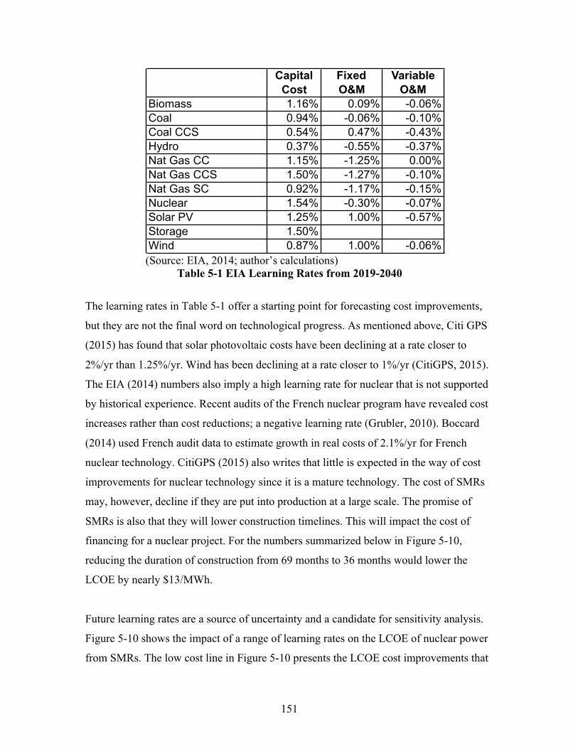
151

(Source: EIA, 2014; author’s calculations)

Table 5-1 EIA Learning Rates from 2019-2040

The learning rates in Table 5-1 offer a starting point for forecasting cost improvements,

but they are not the final word on technological progress. As mentioned above, Citi GPS

(2015) has found that solar photovoltaic costs have been declining at a rate closer to

2%/yr than 1.25%/yr. Wind has been declining at a rate closer to 1%/yr (CitiGPS, 2015).

The EIA (2014) numbers also imply a high learning rate for nuclear that is not supported

by historical experience. Recent audits of the French nuclear program have revealed cost

increases rather than cost reductions; a negative learning rate (Grubler, 2010). Boccard

(2014) used French audit data to estimate growth in real costs of 2.1%/yr for French

nuclear technology. CitiGPS (2015) also writes that little is expected in the way of cost

improvements for nuclear technology since it is a mature technology. The cost of SMRs

may, however, decline if they are put into production at a large scale. The promise of

SMRs is also that they will lower construction timelines. This will impact the cost of

financing for a nuclear project. For the numbers summarized below in Figure 5-10,

reducing the duration of construction from 69 months to 36 months would lower the

LCOE by nearly $13/MWh.

Future learning rates are a source of uncertainty and a candidate for sensitivity analysis.

Figure 5-10 shows the impact of a range of learning rates on the LCOE of nuclear power

from SMRs. The low cost line in Figure 5-10 presents the LCOE cost improvements that

Capital Cost

Fixed O&M

Variable O&M

Biomass 1.16% 0.09% -0.06%Coal 0.94% -0.06% -0.10%Coal CCS 0.54% 0.47% -0.43%Hydro 0.37% -0.55% -0.37%Nat Gas CC 1.15% -1.25% 0.00%Nat Gas CCS 1.50% -1.27% -0.10%Nat Gas SC 0.92% -1.17% -0.15%Nuclear 1.54% -0.30% -0.07%Solar PV 1.25% 1.00% -0.57%Storage 1.50%Wind 0.87% 1.00% -0.06%

152

would result from the EIA (2015) learning rate of 1.5%. The high cost line presents the

impact of negative learning at -1.5%. Cost increases in France’s nuclear program were

driven by safety concerns (Cooper, 2014). Safeguards against nuclear accident have made

nuclear designs more complex and this has increased costs. Cooper (2014) argues that

this is an inherent property of nuclear power systems, which rely on a “catastrophically

dangerous resource that is vulnerable to human frailties and the vicissitudes of Mother

Nature” (Cooper, 2014: 174). On the other hand, wind and solar electricity generation

technologies are considered relatively benign. Their components are amenable to mass

production, which can create economies of scale in the manufacturing process. These

attributes have likely contributed to the rapid decline of solar photovoltaic costs but it

remains unclear how long they will continue and at what rate. I consider a range of

learning rates in the sensitivity analysis of scenario costs in Chapter 8.

Financing Costs

There are costs associated with obtaining the necessary funds for capital projects. In their

latest Annual Report, SaskPower notes that it “raises most of its capital through internal

operating activities and through borrowings obtained from the Government of

Saskatchewan Ministry of Finance” (SaskPower, 2015: 67). In 2014 SaskPower had

$4250 million in recourse debt obtained as advances from the Government of

Saskatchewan’s General Revenue Fund (GRF).51 The province currently sits in a

relatively strong financial position and as such is able to access low cost debt financing.

In both 2013 and 2014 the Government of Saskatchewan had a credit rating of AA on

long-term debt obligations (SaskPower, 2015: 67). In the low-interest environment of

2014, SaskPower was able to obtain long-term financing of $675 million at effective

interest rates that varied from 3.43% to 3.95% (SaskPower, 2015: 70).52 As a Crown

Corporation, SaskPower is wholly owned by the Government of Saskatchewan through

51 Note that the term for most of SaskPower’s debt is approximately 30 years from the date of issue. 52 SaskPower also accessed $100 million in financing at a floating interest rate and borrowed “$86 million in short-term advances” from “the Government of Saskatchewan’s General Revenue Fund” with “interest rates ranging from .997% to 1% and maturity within 2015 (SaskPower, 2015: 70).

153

the Crown Investment Corporation (CIC). CIC issues equity advances to SaskPower. As

of December 31st, 2014 SaskPower had $660 million in equity advances from CIC.

SaskPower has a long-term target for return on equity of 8.5% (SaskPower, 2015: 39).

However, due to the need for substantial investment in the Saskatchewan electricity

system the Government of Saskatchewan has opted not to take dividends from

SaskPower for the foreseeable future. It seems appropriate therefore to model the cost of

capital as consisting entirely of debt financing at 4%/yr interest, a rate slightly higher

than the current low interest rates charged for long-term debt and which anticipates the

possibility of a rate increase.53

Private power producers do not have access to the favourable financing terms that

SaskPower receives, and instead have higher return on equity targets for their

shareholders. This means that private power projects will face higher financing charges.

This has implications for the comparative costs of public versus private construction. In

the SIM model I make the simplifying assumption that all new capital is constructed by

SaskPower.

Financing costs also include interest that accumulates on capital during the construction

period. Technologies with long construction periods such as nuclear and coal-fired plants

will accumulate more interest. I add interest incurred during the construction period to the

capital cost and amortize the whole amount over the expected lifetime of the technology.

Details on my methodology can be found in Appendix 5A.

Other Costs

There are other technology-specific costs that can be considered in a calculation of

LCOE:

53 SaskPower had a debt-equity ratio of 73.5% as of December 31, 2014, meaning that debt financing currently accounts for 73.5% of total financing. This is a change from December 31st, 2013 when the debt-equity ratio was 69.8%. This number is forecast to continue to creep upwards; by 2017 the debt ratio (%) target is 77.3%. This reflects the period of intensive investment currently occurring at SaskPower. (SaskPower, 2015)

154

• In Saskatchewan, hydroelectric facilities pay water royalties at a rate of

$5.10/MWh electricity generated (Interview 24). I assume this cost is included in

the variable operations and maintenance cost of hydroelectricity, which I have set

at $7.20/MWh;

• All facilities will also incur decommissioning charges at the end of their life.

Nuclear power plants require especially large decommissioning costs due to the

hazard of radioactivity. Boccard (2014) estimates that decommissioning of French

nuclear reactors will cost 25% of the original investment cost. Due to a lack of

data I have not included decommissioning costs, which would appear to favour, in

relative terms, nuclear power;

• Nuclear power plants must also pay for the long-term storage of spent nuclear

fuel. EPRI (2013) adds $1/MWh to the variable operations and maintenance

(O&M) costs of nuclear power plants to represent the amount that would be paid

to a nuclear waste management organization. Canada’s Nuclear Waste

Management Organization makes the same estimate for the cost of long-term

waste disposal (NWMO, 2015). I have used a variable O&M cost for nuclear on

par with EPRI (2013).;

• Fossil fuel plants emit pollutants beside CO2. Coal plants in particular emit

sulphur dioxide (SO2), particulates, and mercury. DSS (2005) quantified the

health impacts resulting from these pollutants in Ontario and found the health

costs of an electricity futures scenario that maintained the Ontario electricity

generation mix at the status quo proportions that existed in 2005 – which included

a substantial amount of coal-fired generation – to be three times higher than the

financial cost. I have not included health costs in the LCOE figures below, which

means that the fossil-fuel costs are conservative estimates.

• The use of carbon dioxide (CO2) for enhanced oil recovery (EOR) will produce

oil that has a 10.8% higher GHG intensity than an average barrel of conventional

oil, but 11.5% lower GHG intensity than oil extracted from the oil sands. The

EOR operation will also lead to CO2 emissions on-site. This leads to “a net on-site

storage of .696 TCO2e per 1 TCO2e brought to the site” (Wong et al., 2013: 8). I

155

do not consider the GHG implications of EOR in this analysis. (Wong et al.,

2013)

Other Benefits

Part of the motivation for the Boundary Dam III carbon capture and storage (CCS)

project was to provide a source of CO2 for enhanced oil recovery (EOR) (IEAGHG,

2015). SaskPower sells CO2 to the oil company Cenovus for around $22.50/tonne CO2

(Glennie, 2015). This represents a potential revenue stream for the Boundary Dam

project.54 In Figure 5-10 I include two measures of LCOE for Boundary Dam with

(SaskPower Low) and without (SaskPower High) the revenue from sales of CO2.

SaskPower is also able to sell sulphuric acid from the Boundary Dam project. The

revenue from these sales is limited (Glennie, 2015) and I have excluded it from the

LCOE calculations.

Cost Assumptions

I gathered electricity cost information from published estimates of Saskatchewan built

projects and the energy cost literature (EIA, 2015; Lazard, 2014; EPRI, 2013). I adjusted

all costs to Canadian 2014 constant dollars using U.S. exchange rate data from the Bank

of Canada (Bank of Canada, 2015) and the Canadian All-items Consumer Price Index

(Statistics Canada, 2015 CANSIM Table 326-0020).

The initial LCOE calculations for coal and natural gas fired plants (shown below in

Figure 5-10) assume constant fuel prices equivalent to current rates ($4.22/GJ for natural

gas and $23.18/tonne for lignite coal). They are thus conservative estimates as fuel prices

54 This potential source of revenue can also be a financial liability. SaskPower has signed a contract with Cenovus to deliver a certain quantity of CO2 for enhanced oil recovery. If SaskPower cannot deliver the CO2 and meet its contractual obligations it must pay a penalty to Cenovus. This occurred in 2014 and 2015 when – due to technical problems at the new plant – Boundary Dam III has operated at less than full capacity. This has meant that SaskPower has only been apply to supply half of the 800 kilotonnes of CO2 is was supposed to provide Cenovus in 2015. By October 2015 SaskPower had paid $12 million in penalties to Cenovus and was on track to face another $5-6 million in penalties by the end of 2015. (Leo, 2015)

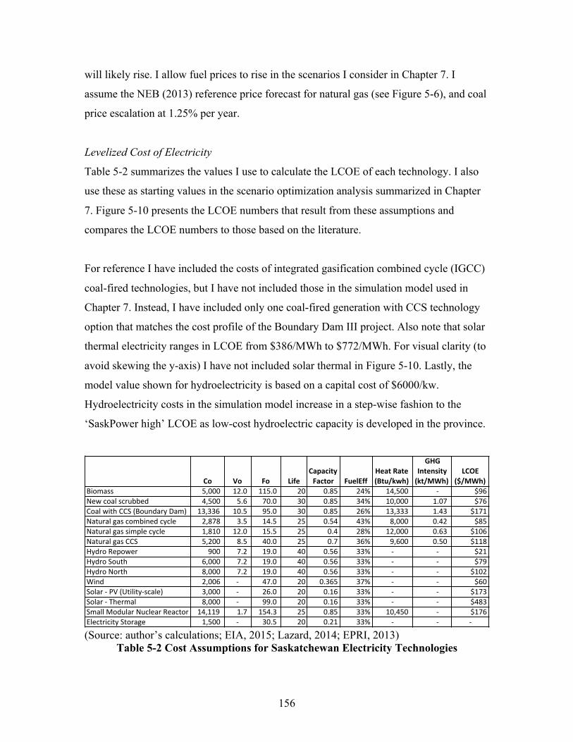
156

will likely rise. I allow fuel prices to rise in the scenarios I consider in Chapter 7. I

assume the NEB (2013) reference price forecast for natural gas (see Figure 5-6), and coal

price escalation at 1.25% per year.

Levelized Cost of Electricity

Table 5-2 summarizes the values I use to calculate the LCOE of each technology. I also

use these as starting values in the scenario optimization analysis summarized in Chapter

7. Figure 5-10 presents the LCOE numbers that result from these assumptions and

compares the LCOE numbers to those based on the literature.

For reference I have included the costs of integrated gasification combined cycle (IGCC)

coal-fired technologies, but I have not included those in the simulation model used in

Chapter 7. Instead, I have included only one coal-fired generation with CCS technology

option that matches the cost profile of the Boundary Dam III project. Also note that solar

thermal electricity ranges in LCOE from $386/MWh to $772/MWh. For visual clarity (to

avoid skewing the y-axis) I have not included solar thermal in Figure 5-10. Lastly, the

model value shown for hydroelectricity is based on a capital cost of $6000/kw.

Hydroelectricity costs in the simulation model increase in a step-wise fashion to the

‘SaskPower high’ LCOE as low-cost hydroelectric capacity is developed in the province.

(Source: author’s calculations; EIA, 2015; Lazard, 2014; EPRI, 2013)

Table 5-2 Cost Assumptions for Saskatchewan Electricity Technologies

Co Vo Fo LifeCapacity.Factor FuelEff

Heat.Rate.(Btu/kwh)

GHG.Intensity.(kt/MWh)

LCOE.($/MWh)

Biomass 5,000**** 12.0*** 115.0** 20 0.85 24% 14,500****** 1*********** $96New*coal*scrubbed 4,500**** 5.6***** 70.0**** 30 0.85 34% 10,000****** 1.07********* $76Coal*with*CCS*(Boundary*Dam) 13,336** 10.5*** 95.0**** 30 0.85 26% 13,333****** 1.43********* $171Natural*gas*combined*cycle 2,878**** 3.5***** 14.5**** 25 0.54 43% 8,000******** 0.42********* $85Natural*gas*simple*cycle 1,810**** 12.0*** 15.5**** 25 0.4 28% 12,000****** 0.63********* $106Natural*gas*CCS 5,200**** 8.5***** 40.0**** 25 0.7 36% 9,600******** 0.50********* $118Hydro*Repower 900******** 7.2***** 19.0**** 40 0.56 33% 1 1*********** $21Hydro*South 6,000**** 7.2***** 19.0**** 40 0.56 33% 1 1*********** $79Hydro*North 8,000**** 7.2***** 19.0**** 40 0.56 33% 1 1*********** $102Wind 2,006**** 1***** 47.0**** 20 0.365 37% 1 1*********** $60Solar*1*PV*(Utility1scale) 3,000**** 1***** 26.0**** 20 0.16 33% 1 1*********** $173Solar*1*Thermal 8,000**** 1***** 99.0**** 20 0.16 33% 1 1*********** $483Small*Modular*Nuclear*Reactor 14,119** 1.7***** 154.3** 25 0.85 33% 10,450****** 1*********** $176Electricity*Storage 1,500**** 1***** 30.5**** 20 0.21 33% 1 1*********** 1

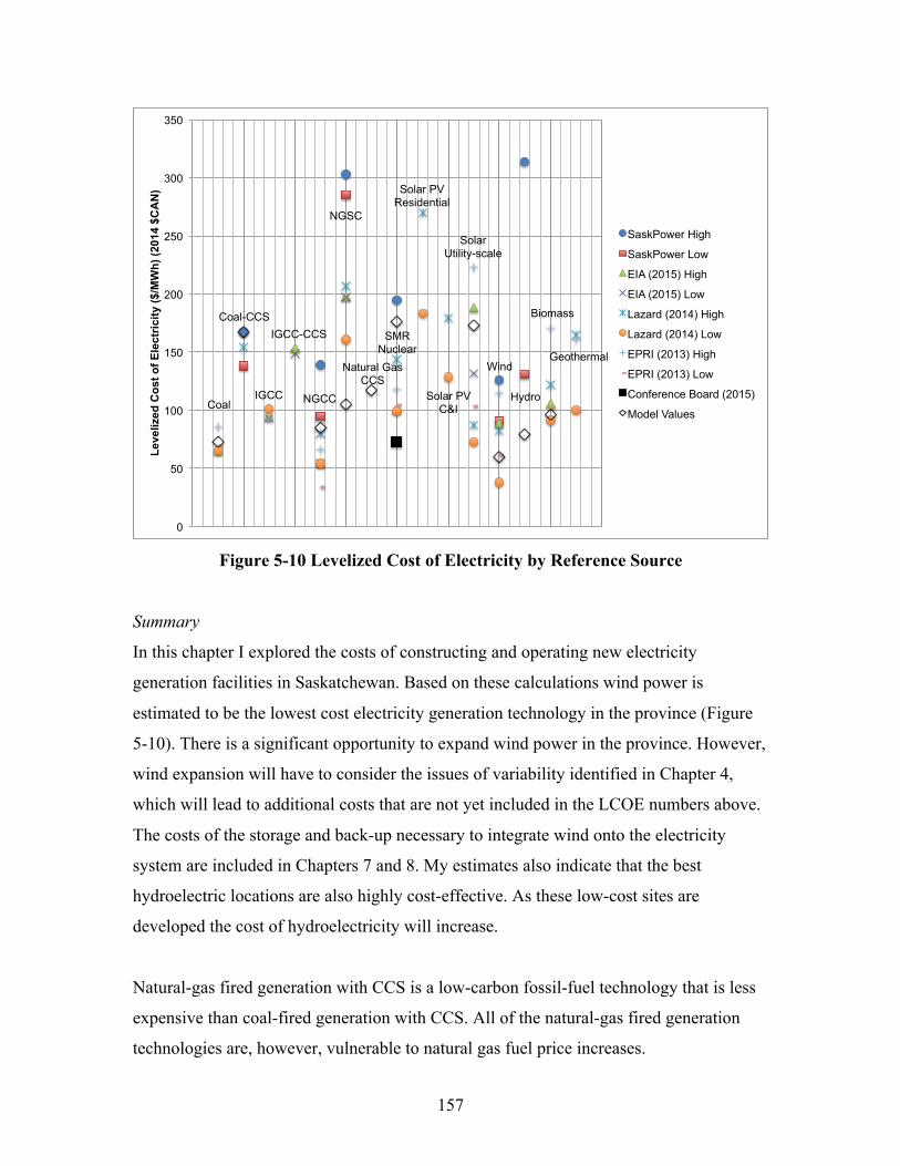
157

Figure 5-10 Levelized Cost of Electricity by Reference Source

Summary

In this chapter I explored the costs of constructing and operating new electricity

generation facilities in Saskatchewan. Based on these calculations wind power is

estimated to be the lowest cost electricity generation technology in the province (Figure

5-10). There is a significant opportunity to expand wind power in the province. However,

wind expansion will have to consider the issues of variability identified in Chapter 4,

which will lead to additional costs that are not yet included in the LCOE numbers above.

The costs of the storage and back-up necessary to integrate wind onto the electricity

system are included in Chapters 7 and 8. My estimates also indicate that the best

hydroelectric locations are also highly cost-effective. As these low-cost sites are

developed the cost of hydroelectricity will increase.

Natural-gas fired generation with CCS is a low-carbon fossil-fuel technology that is less

expensive than coal-fired generation with CCS. All of the natural-gas fired generation

technologies are, however, vulnerable to natural gas fuel price increases.

Coal-CCS

NGSC

Hydro Coal

IGCC

IGCC-CCS

NGCC

Solar Utility-scale

SMR Nuclear

Solar PV Residential

Solar PV C&I

Wind Geothermal

Natural Gas CCS

Biomass

0

50

100

150

200

250

300

350

Leve

lized

Cos

t of E

lect

rici

ty ($

/MW

h) (2

014

$CA

N)

SaskPower High

SaskPower Low

EIA (2015) High

EIA (2015) Low

Lazard (2014) High

Lazard (2014) Low

EPRI (2013) High

EPRI (2013) Low

Conference Board (2015)

Model Values

158

Other low-carbon technologies such as coal-fired generation with CCS and nuclear power

are estimated to be considerably more expensive than the current wholesale price of

power, which lies between $50/MWh and $70/MWh for large electricity customers

(SaskPower, 2015). Utility-scale solar power is notably on par with coal-fired generation

with CCS and small, modular nuclear reactors. Solar costs are also falling rapidly

suggesting that solar will likely soon be less expensive than either of these technologies.

Solar, like wind, does require a system designed for variability. The costs of integrating

solar are included in the scenarios outlined in Chapters 7 and 8, but are excluded from the

LCOE numbers in Figure 5-10.

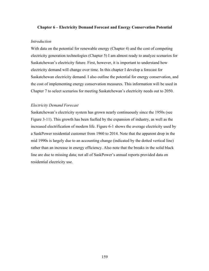
159

Chapter 6 – Electricity Demand Forecast and Energy Conservation Potential

Introduction

With data on the potential for renewable energy (Chapter 4) and the cost of competing

electricity generation technologies (Chapter 5) I am almost ready to analyze scenarios for

Saskatchewan’s electricity future. First, however, it is important to understand how

electricity demand will change over time. In this chapter I develop a forecast for

Saskatchewan electricity demand. I also outline the potential for energy conservation, and

the cost of implementing energy conservation measures. This information will be used in

Chapter 7 to select scenarios for meeting Saskatchewan’s electricity needs out to 2050.

Electricity Demand Forecast

Saskatchewan’s electricity system has grown nearly continuously since the 1950s (see

Figure 3-11). This growth has been fuelled by the expansion of industry, as well as the

increased electrification of modern life. Figure 6-1 shows the average electricity used by

a SaskPower residential customer from 1960 to 2014. Note that the apparent drop in the

mid 1990s is largely due to an accounting change (indicated by the dotted vertical line)

rather than an increase in energy efficiency. Also note that the breaks in the solid black

line are due to missing data; not all of SaskPower’s annual reports provided data on

residential electricity use.

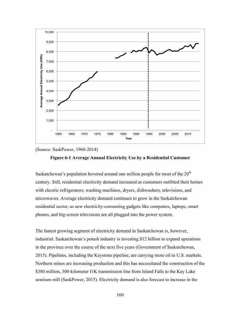
160

(Source: SaskPower, 1960-2014)

Figure 6-1 Average Annual Electricity Use by a Residential Customer

Saskatchewan’s population hovered around one million people for most of the 20th

century. Still, residential electricity demand increased as customers outfitted their homes

with electric refrigerators, washing machines, dryers, dishwashers, televisions, and

microwaves. Average electricity demand continues to grow in the Saskatchewan

residential sector, as new electricity-consuming gadgets like computers, laptops, smart

phones, and big-screen televisions are all plugged into the power system.

The fastest growing segment of electricity demand in Saskatchewan is, however,

industrial. Saskatchewan’s potash industry is investing $12 billion to expand operations

in the province over the course of the next five years (Government of Saskatchewan,

2015). Pipelines, including the Keystone pipeline, are carrying more oil to U.S. markets.

Northern mines are increasing production and this has necessitated the construction of the

$380 million, 300-kilometer I1K transmission line from Island Falls to the Key Lake

uranium mill (SaskPower, 2015). Electricity demand is also forecast to increase in the

-

1,000

2,000

3,000

4,000

5,000

6,000

7,000

8,000

9,000

10,000

1960 1965 1970 1975 1980 1985 1990 1995 2000 2005 2010

Aver

age

Ann

ual E

lect

ricity

Use

(kW

h)

Year

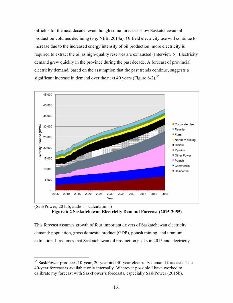
161

oilfields for the next decade, even though some forecasts show Saskatchewan oil

production volumes declining (e.g. NEB, 2014a). Oilfield electricity use will continue to

increase due to the increased energy intensity of oil production; more electricity is

required to extract the oil as high-quality reserves are exhausted (Interview 5). Electricity

demand grew quickly in the province during the past decade. A forecast of provincial

electricity demand, based on the assumption that the past trends continue, suggests a

significant increase in demand over the next 40 years (Figure 6-2).55

(SaskPower, 2015b; author’s calculations)

Figure 6-2 Saskatchewan Electricity Demand Forecast (2015-2055)

This forecast assumes growth of four important drivers of Saskatchewan electricity

demand: population, gross domestic product (GDP), potash mining, and uranium

extraction. It assumes that Saskatchewan oil production peaks in 2015 and electricity

55 SaskPower produces 10-year, 20-year and 40-year electricity demand forecasts. The 40-year forecast is available only internally. Wherever possible I have worked to calibrate my forecast with SaskPower’s forecasts, especially SaskPower (2015b).

-

5,000

10,000

15,000

20,000

25,000

30,000

35,000

40,000

45,000

2005 2010 2015 2020 2025 2030 2035 2040 2045 2050 2055

Elec

tric

ity D

eman

d (G

Wh)

Year

Corporate Use

Reseller

Farm

Northern Mining

Oilfield

Pipeline

Other Power

Potash

Commercial

Residential

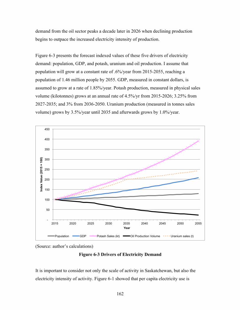
162

demand from the oil sector peaks a decade later in 2026 when declining production

begins to outpace the increased electricity intensity of production.

Figure 6-3 presents the forecast indexed values of these five drivers of electricity

demand: population, GDP, and potash, uranium and oil production. I assume that

population will grow at a constant rate of .6%/year from 2015-2055, reaching a

population of 1.46 million people by 2055. GDP, measured in constant dollars, is

assumed to grow at a rate of 1.85%/year. Potash production, measured in physical sales

volume (kilotonnes) grows at an annual rate of 4.5%/yr from 2015-2026; 3.25% from

2027-2035; and 3% from 2036-2050. Uranium production (measured in tonnes sales

volume) grows by 3.5%/year until 2035 and afterwards grows by 1.0%/year.

(Source: author’s calculations)

Figure 6-3 Drivers of Electricity Demand

It is important to consider not only the scale of activity in Saskatchewan, but also the

electricity intensity of activity. Figure 6-1 showed that per capita electricity use is

-

50

100

150

200

250

300

350

400

450

2015 2020 2025 2030 2035 2040 2045 2050 2055

Inde

x Va

lue

(201

5 =

100)

Year

Population GDP Potash Sales (kt) Oil Production Volume Uranium sales (t)

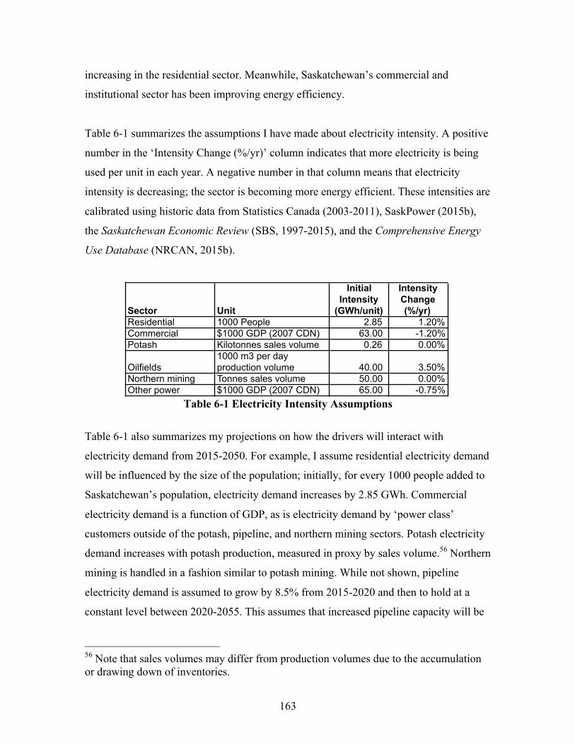
163

increasing in the residential sector. Meanwhile, Saskatchewan’s commercial and

institutional sector has been improving energy efficiency.

Table 6-1 summarizes the assumptions I have made about electricity intensity. A positive

number in the ‘Intensity Change (%/yr)’ column indicates that more electricity is being

used per unit in each year. A negative number in that column means that electricity

intensity is decreasing; the sector is becoming more energy efficient. These intensities are

calibrated using historic data from Statistics Canada (2003-2011), SaskPower (2015b),

the Saskatchewan Economic Review (SBS, 1997-2015), and the Comprehensive Energy

Use Database (NRCAN, 2015b).

Table 6-1 Electricity Intensity Assumptions

Table 6-1 also summarizes my projections on how the drivers will interact with

electricity demand from 2015-2050. For example, I assume residential electricity demand

will be influenced by the size of the population; initially, for every 1000 people added to

Saskatchewan’s population, electricity demand increases by 2.85 GWh. Commercial

electricity demand is a function of GDP, as is electricity demand by ‘power class’

customers outside of the potash, pipeline, and northern mining sectors. Potash electricity

demand increases with potash production, measured in proxy by sales volume.56 Northern

mining is handled in a fashion similar to potash mining. While not shown, pipeline

electricity demand is assumed to grow by 8.5% from 2015-2020 and then to hold at a

constant level between 2020-2055. This assumes that increased pipeline capacity will be

56 Note that sales volumes may differ from production volumes due to the accumulation or drawing down of inventories.

Sector Unit

Initial Intensity

(GWh/unit)

Intensity Change (%/yr)

Residential 1000 People 2.85 1.20%Commercial $1000 GDP (2007 CDN) 63.00 -1.20%Potash Kilotonnes sales volume 0.26 0.00%

Oilfields1000 m3 per day production volume 40.00 3.50%

Northern mining Tonnes sales volume 50.00 0.00%Other power $1000 GDP (2007 CDN) 65.00 -0.75%

164

built (e.g. the proposed Energy East pipeline) and a continued high volume of oil exports

from Alberta after 2020.

The remaining categories of electricity demand are forecast as follows:

• Farm electricity demand is constant at 1300 GWh per year; this category of

electricity demand has been falling slowly in recent years as small family farms

have been purchased and amalgamated into large corporate farms. This has meant

fewer people living on farms in rural Saskatchewan;

• Reseller electricity demand refers to the electricity sold to Saskatoon Light &

Power and Swift Current Light & Power. These companies manage electricity

distribution in their respective cities. However, Saskatoon Light & Power sells

only to customers within the 1958 city boundaries of Saskatoon; customers

outside of this area are served by SaskPower. Electricity demand from these

resellers has grown slowly in recent years. I assume that electricity demand grows

at half the rate of population growth. This means that reseller electricity demand

grows from 1300 GWh in 2015 to 1480 GWh in 2055;

• Corporate Use refers to electricity used within SaskPower’s operations. This is a

relatively small portion of electricity demand. Based on historic data I assume that

corporate use equals .4% of the total electricity demand from the other categories;

• Line Loss refers to electricity lost through the transmission and distribution of

electricity. Based on the historic relationship between electricity demand and line

loss I assume that line loss is equal to 7.5% of total electricity demand (including

corporate use).

This forecast is by no means certain. The United States government recently said no to

the Keystone XL pipeline project and similar opposition in Canada could prevent the

Energy East pipeline from being built. Strong climate policy could encourage fuel

switching away from fossil fuels and lower demand for Alberta oil. In the potash sector,

demand has been cooling in 2015 and PotashCorp has announced a round of lay-offs and

temporary shutdowns at three Saskatchewan plants (CBC, 2015d). Lower oil and potash

demand would result in a lower electricity demand forecast. Conversely, the forecast

165

would be higher with stronger growth in commodity sales. Higher penetrations of electric

vehicles would also increase electricity demand. The forecast used in this dissertation

provides one possible demand scenario, and one possible set of drivers that would

achieve the scenario. Other demand scenarios are possible.

Electricity Conservation Potential

SaskPower produces two electricity demand forecasts: one that considers opportunities to

conserve electricity through ‘demand side-management’ (DSM), and another that

excludes the potential for energy conservation. ICF-Marbek (2011) defines DSM as

follows,

“DSM measures can include energy efficiency (use more efficiently),

energy conservation (use less), demand management (use less during peak

periods), fuel switching (use a different fuel to provide the energy service)

and customer-side generation (displace load off of grid).” 57 (p. 5)

The forecast presented in Figure 6-1 is calibrated to SaskPower’s (2015b) DSM-adjusted

forecast. This forecast is informed by the efforts of SaskPower’s Customer Services

Branch, which designs and implements SaskPower’s energy conservation programming

(Interview 14). This conservation programming is in turn informed by ICF-Marbek’s

(2011) Conservation Potential Review for Saskatchewan. In 2010-2011 SaskPower

commissioned ICF-Marbek to conduct a review of conservation potential in

Saskatchewan. The results of this review are presented in Tables 6-2 and 6-3.58 Table 6-2

indicates the potential for peak demand savings (expressed in megawatts). Table 6-3

indicates the potential to reduce total electricity demand in Saskatchewan (in gigawatt-

hours/year).

57 Note that demand management does not necessarily mean using less electricity, but instead involves shifting demand away from periods of high or “peak” demand. 58 The Residential (Resl) sector includes residential homes and farm households. The commercial sector (Comml) includes commercial and institutional customers. The industrial sector (Indl) includes large power users such as mines and oilfield customers. (ICF-Marbek, 2011)

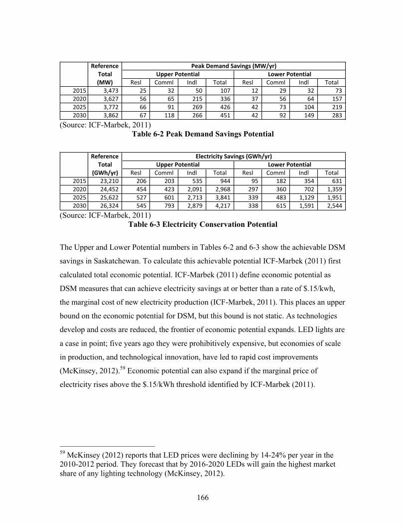
166

(Source: ICF-Marbek, 2011)

Table 6-2 Peak Demand Savings Potential

(Source: ICF-Marbek, 2011)

Table 6-3 Electricity Conservation Potential

The Upper and Lower Potential numbers in Tables 6-2 and 6-3 show the achievable DSM

savings in Saskatchewan. To calculate this achievable potential ICF-Marbek (2011) first

calculated total economic potential. ICF-Marbek (2011) define economic potential as

DSM measures that can achieve electricity savings at or better than a rate of $.15/kwh,

the marginal cost of new electricity production (ICF-Marbek, 2011). This places an upper

bound on the economic potential for DSM, but this bound is not static. As technologies

develop and costs are reduced, the frontier of economic potential expands. LED lights are

a case in point; five years ago they were prohibitively expensive, but economies of scale

in production, and technological innovation, have led to rapid cost improvements

(McKinsey, 2012).59 Economic potential can also expand if the marginal price of

electricity rises above the $.15/kWh threshold identified by ICF-Marbek (2011).

59 McKinsey (2012) reports that LED prices were declining by 14-24% per year in the 2010-2012 period. They forecast that by 2016-2020 LEDs will gain the highest market share of any lighting technology (McKinsey, 2012).

ReferenceTotal(MW) Resl Comml Indl Total Resl Comml Indl Total

2015 3,473666666666 256666666666 326666666666 506666666666 10766666666 126666666666 296666666666 326666666666 7366666666662020 3,627666666666 566666666666 656666666666 21566666666 33666666666 376666666666 566666666666 646666666666 157666666662025 3,772666666666 666666666666 916666666666 26966666666 42666666666 426666666666 736666666666 10466666666 219666666662030 3,862666666666 676666666666 11866666666 26666666666 45166666666 426666666666 926666666666 14966666666 28366666666

Peak2Demand2Savings2(MW/yr)Upper2Potential Lower2Potential

ReferenceTotal

(GWh/yr) Resl Comml Indl Total Resl Comml Indl Total2015 23,2104444444 20644444444 20344444444 53544444444 94444444444 954444444444 18244444444 35444444444 631444444442020 24,4524444444 45444444444 42344444444 2,09144444 2,96844444 29744444444 36044444444 70244444444 1,359444442025 25,6224444444 52744444444 60144444444 2,71344444 3,84144444 33944444444 48344444444 1,12944444 1,951444442030 26,3244444444 54544444444 79344444444 2,87944444 4,21744444 33844444444 61544444444 1,59144444 2,54444444

Electricity5Savings5(GWh/yr)Upper5Potential Lower5Potential

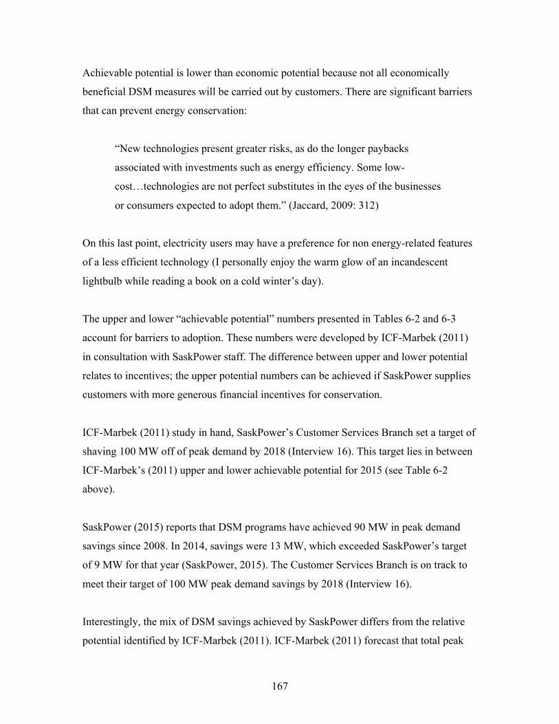
167

Achievable potential is lower than economic potential because not all economically

beneficial DSM measures will be carried out by customers. There are significant barriers

that can prevent energy conservation:

“New technologies present greater risks, as do the longer paybacks

associated with investments such as energy efficiency. Some low-

cost…technologies are not perfect substitutes in the eyes of the businesses

or consumers expected to adopt them.” (Jaccard, 2009: 312)

On this last point, electricity users may have a preference for non energy-related features

of a less efficient technology (I personally enjoy the warm glow of an incandescent

lightbulb while reading a book on a cold winter’s day).

The upper and lower “achievable potential” numbers presented in Tables 6-2 and 6-3

account for barriers to adoption. These numbers were developed by ICF-Marbek (2011)

in consultation with SaskPower staff. The difference between upper and lower potential

relates to incentives; the upper potential numbers can be achieved if SaskPower supplies

customers with more generous financial incentives for conservation.

ICF-Marbek (2011) study in hand, SaskPower’s Customer Services Branch set a target of

shaving 100 MW off of peak demand by 2018 (Interview 16). This target lies in between

ICF-Marbek’s (2011) upper and lower achievable potential for 2015 (see Table 6-2

above).

SaskPower (2015) reports that DSM programs have achieved 90 MW in peak demand

savings since 2008. In 2014, savings were 13 MW, which exceeded SaskPower’s target

of 9 MW for that year (SaskPower, 2015). The Customer Services Branch is on track to

meet their target of 100 MW peak demand savings by 2018 (Interview 16).

Interestingly, the mix of DSM savings achieved by SaskPower differs from the relative

potential identified by ICF-Marbek (2011). ICF-Marbek (2011) forecast that total peak

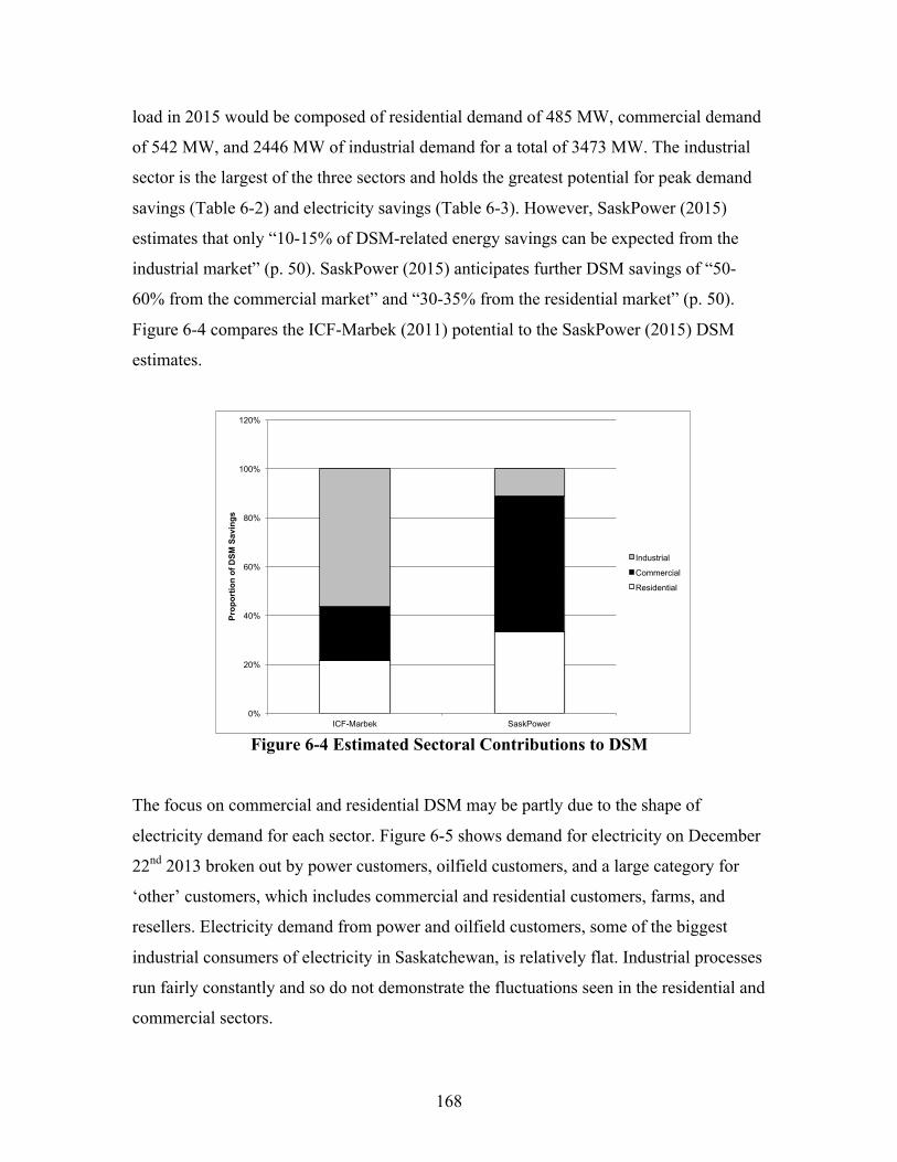
168

load in 2015 would be composed of residential demand of 485 MW, commercial demand

of 542 MW, and 2446 MW of industrial demand for a total of 3473 MW. The industrial

sector is the largest of the three sectors and holds the greatest potential for peak demand

savings (Table 6-2) and electricity savings (Table 6-3). However, SaskPower (2015)

estimates that only “10-15% of DSM-related energy savings can be expected from the

industrial market” (p. 50). SaskPower (2015) anticipates further DSM savings of “50-

60% from the commercial market” and “30-35% from the residential market” (p. 50).

Figure 6-4 compares the ICF-Marbek (2011) potential to the SaskPower (2015) DSM

estimates.

Figure 6-4 Estimated Sectoral Contributions to DSM

The focus on commercial and residential DSM may be partly due to the shape of

electricity demand for each sector. Figure 6-5 shows demand for electricity on December

22nd 2013 broken out by power customers, oilfield customers, and a large category for

‘other’ customers, which includes commercial and residential customers, farms, and

resellers. Electricity demand from power and oilfield customers, some of the biggest

industrial consumers of electricity in Saskatchewan, is relatively flat. Industrial processes

run fairly constantly and so do not demonstrate the fluctuations seen in the residential and

commercial sectors.

0%

20%

40%

60%

80%

100%

120%

ICF-Marbek SaskPower

Pro

port

ion

of D

SM

Sav

ings

Industrial

Commercial

Residential

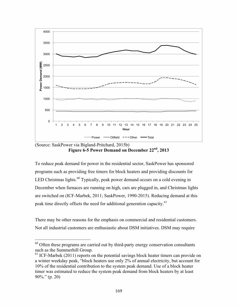
169

(Source: SaskPower via Bigland-Pritchard, 2015b)

Figure 6-5 Power Demand on December 22nd, 2013

To reduce peak demand for power in the residential sector, SaskPower has sponsored

programs such as providing free timers for block heaters and providing discounts for

LED Christmas lights.60 Typically, peak power demand occurs on a cold evening in

December when furnaces are running on high, cars are plugged in, and Christmas lights

are switched on (ICF-Marbek, 2011; SaskPower, 1990-2015). Reducing demand at this

peak time directly offsets the need for additional generation capacity.61

There may be other reasons for the emphasis on commercial and residential customers.

Not all industrial customers are enthusiastic about DSM initiatives. DSM may require

60 Often these programs are carried out by third-party energy conservation consultants such as the Summerhill Group. 61 ICF-Marbek (2011) reports on the potential savings block heater timers can provide on a winter weekday peak, “block heaters use only 2% of annual electricity, but account for 10% of the residential contribution to the system peak demand. Use of a block heater timer was estimated to reduce the system peak demand from block heaters by at least 90%.” (p. 20)

0

500

1000

1500

2000

2500

3000

3500

4000

1 2 3 4 5 6 7 8 9 10 11 12 13 14 15 16 17 18 19 20 21 22 23 24 25

Pow

er D

eman

d (M

W)

Hour

Power Oilfield Other Total

170

changes in operating practices that increase other costs. For example, large, inefficient

fans are used to blow air in potash mines. These fans use a lot of power and more

efficient fans are available. However, equipment in a potash mine must be cleaned

frequently to deal with corrosion; the salts in the mines quickly accumulate on

equipment. The large fans are easily cleaned and this saves labour time relative to more

efficient, but smaller and harder to clean, fans. (Interview 21)

Electricity is also a relatively small portion of production costs in Saskatchewan’s potash

mines; from 2003-2011 expenditures on electricity were about one-fifth the level of

expenditures on labour (Statistics Canada, 2003-2011). The electricity cost savings

promised by DSM may not be large enough to allocate scarce labour time to achieving

them.

Increasing electricity prices may change this thinking. SaskPower customers will often

complain when rates increase, and this becomes an ideal time to talk about DSM

opportunities (Interview 36). SaskPower is working to create a “culture of conservation”

within Saskatchewan that will encourage business and industry to react to price increases

with increased efficiency rather than anger (Interview 36).

I now turn my attention to the costs of electricity conservation in Saskatchewan.

The Cost of Electricity Conservation

The cost of electricity conservation measures can be expressed by the Cost of Conserved

Energy (CCE). Marbek (2007) defines CCE,

“CCE is calculated as the annualized incremental cost (including operating

and maintenance) of the measure divided by the annual kilowatt-hour

savings achieved, excluding any administrative or program costs to

achieve full use of the measure.” (p. 5)

171

𝐸𝑞. 6.1 𝐶𝐶𝐸 ($/𝑘𝑊ℎ) = 𝐴𝑛𝑛𝑢𝑎𝑙𝑖𝑧𝑒𝑑 𝐼𝑛𝑐𝑟𝑒𝑚𝑒𝑛𝑡𝑎𝑙 𝐶𝑜𝑠𝑡 ($)

𝐴𝑛𝑛𝑢𝑎𝑙 𝑘𝑊ℎ 𝑠𝑎𝑣𝑖𝑛𝑔𝑠 𝑎𝑐ℎ𝑖𝑒𝑣𝑒𝑑 (𝑘𝑊ℎ)

This measure can be used to compare energy conservation to the cost of generating

electricity (expressed in Chapter 5 using LCOE). Figure 6-6 shows the cost of

conservation in the Saskatchewan residential sector in 2015 as reported by ICF-Marbek

(2011). CCE is indicated by the black ‘marginal cost’ line. Conservation is inexpensive at

low levels of cumulative energy conservation. Costs then increase as “low-hanging fruit”

(i.e. low-cost conservation options) are “picked” (i.e. implemented). Once CCE reaches

$.15/kwh further conservation measures are beyond the realm of economic potential as

defined by ICF-Marbek (2011).

(Source: ICF-Marbek, 2011)

Figure 6-6 Residential DSM Program Costs (Year=2015)

Figure 6-6 shows both the marginal cost of additional conservation efforts (black solid

line) and the average cost of cumulative efforts (green dotted line). The cost of

conserving electricity (CCE) in the residential sector can be lower than many of

0

2

4

6

8

10

12

14

16

0 50 100 150 200

Cos

t (ce

nts/

kWh)

Cumulative Conservation (GWh/yr)

Marginal Cost Average Cost

172

SaskPower’s electricity generation options. Until cumulative electricity savings of about

140 GWh/yr are achieved, the marginal cost of conservation is $.03/kwh or less. This

cost is lower than all of the electricity generation options outlined in Chapter 5.

Conserved electricity is also clean; it avoids greenhouse gas emissions (GHGs).62

SaskPower targets a portfolio of conservation measures that achieve an average cost of

$.03/kwh or less (Interview 8). Average cost is lower than marginal cost because the

presence of low-cost actions in the portfolio balances out the presence of higher cost

actions. The dotted green average cost line in Figure 6-6 shows how average cost

increases with conservation effort. In the residential sector in 2015 it is possible to

achieve a portfolio of actions amounting to about 175 GWh/yr in savings before reaching

an average cost of $.03/kwh.

Figures 6-7 presents the cost of electricity conservation for the commercial sector in

2015. If all the conservation measures that belong to the upper achievable potential

category, which total 206 GWh/yr in 2015, were implemented in the commercial sector,

the average cost of conservation would still be below $.06/kWh. These average costs do

increase in the commercial sector over time (see Table 6-5 below). This is to be expected

as “low-hanging fruit” are “picked”. Average costs also increase as the frontier of

achievable potential expands outwards in future years.

62 At least direct GHGs; energy-saving technologies will contain embodied GHGs.

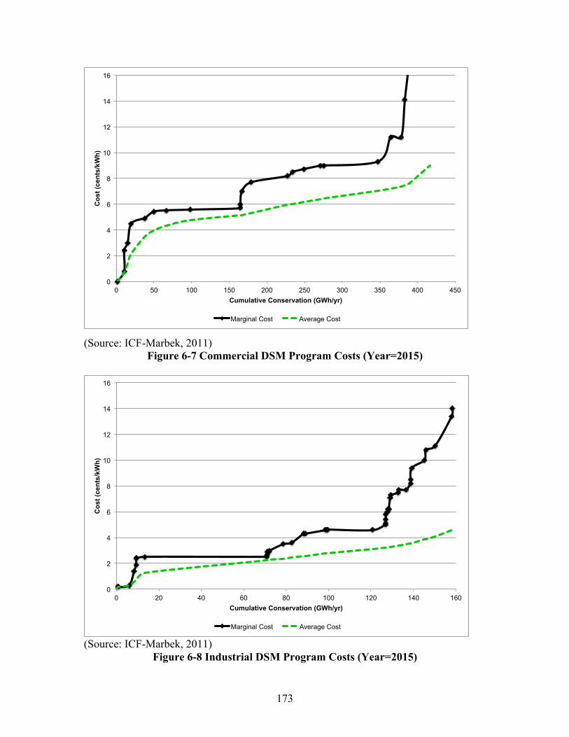
173

(Source: ICF-Marbek, 2011)

Figure 6-7 Commercial DSM Program Costs (Year=2015)

(Source: ICF-Marbek, 2011)

Figure 6-8 Industrial DSM Program Costs (Year=2015)

0

2

4

6

8

10

12

14

16

0 50 100 150 200 250 300 350 400 450

Cos

t (ce

nts/

kWh)

Cumulative Conservation (GWh/yr)

Marginal Cost Average Cost

0

2

4

6

8

10

12

14

16

0 20 40 60 80 100 120 140 160

Cos

t (ce

nts/

kWh)

Cumulative Conservation (GWh/yr)

Marginal Cost Average Cost

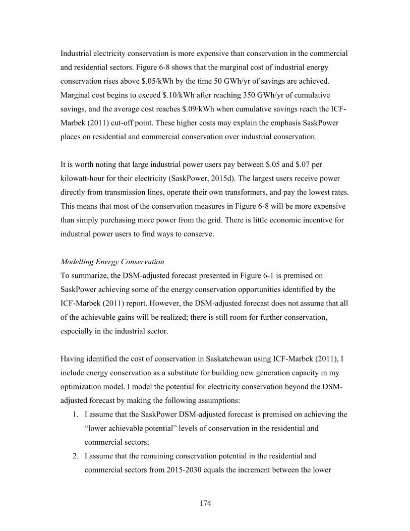
174

Industrial electricity conservation is more expensive than conservation in the commercial

and residential sectors. Figure 6-8 shows that the marginal cost of industrial energy

conservation rises above $.05/kWh by the time 50 GWh/yr of savings are achieved.

Marginal cost begins to exceed $.10/kWh after reaching 350 GWh/yr of cumulative

savings, and the average cost reaches $.09/kWh when cumulative savings reach the ICF-

Marbek (2011) cut-off point. These higher costs may explain the emphasis SaskPower

places on residential and commercial conservation over industrial conservation.

It is worth noting that large industrial power users pay between $.05 and $.07 per

kilowatt-hour for their electricity (SaskPower, 2015d). The largest users receive power

directly from transmission lines, operate their own transformers, and pay the lowest rates.

This means that most of the conservation measures in Figure 6-8 will be more expensive

than simply purchasing more power from the grid. There is little economic incentive for

industrial power users to find ways to conserve.

Modelling Energy Conservation

To summarize, the DSM-adjusted forecast presented in Figure 6-1 is premised on

SaskPower achieving some of the energy conservation opportunities identified by the

ICF-Marbek (2011) report. However, the DSM-adjusted forecast does not assume that all

of the achievable gains will be realized; there is still room for further conservation,

especially in the industrial sector.

Having identified the cost of conservation in Saskatchewan using ICF-Marbek (2011), I

include energy conservation as a substitute for building new generation capacity in my

optimization model. I model the potential for electricity conservation beyond the DSM-

adjusted forecast by making the following assumptions:

1. I assume that the SaskPower DSM-adjusted forecast is premised on achieving the

“lower achievable potential” levels of conservation in the residential and

commercial sectors;

2. I assume that the remaining conservation potential in the residential and

commercial sectors from 2015-2030 equals the increment between the lower

175

achievable potential and the upper achievable potential identified by ICF-Marbek

(2011);

3. After 2030 I assume that residential conservation potential in each 5-year time

step equals 3% of the electricity forecast total for the residential sector. Included

in the residential sector total are the residential sector plus farm electricity

demand plus half of reseller demand;

4. After 2030 I assume that commercial conservation potential in each 5-year time

step equals 3.5% of the electricity forecast total for the commercial sector.

Included in the commercial sector total are the commercial sector plus half the

reseller demand plus one quarter of ‘other power user’ demand. I include 25% of

the ‘other power user’ because the category includes large institutions such as the

University of Regina and the University of Saskatchewan;

5. I assume that the DSM-adjusted forecast (SaskPower, 2015b) includes industrial

conservation only for measures with a marginal cost less than $.05/kWh. From

2015-2030 I subtract the cumulative savings that cost less than $.05/kWh from the

upper achievable potential to determine the remaining conservation potential in

the industrial sector;

6. After 2030 I assume that industrial conservation potential in each 5-year time step

equals 16% of the electricity forecast total for the industrial sector. This large

number indicates the high degree of potential ICF-Marbek (2011) identified in the

industrial sector. I assume the industrial sector is composed of the oilfields, the

potash mining, northern mining and pipeline sectors, and three quarters of the

‘other power user’ sector.

For each sector I represent the cost of electricity conservation as the average cost of the

portfolio of conservation measures that reach the upper achievable potential identified by

ICF-Marbek (2011). In the scenarios outlined in Chapter 7, each GWh of conservation

potential must be purchased at this average cost. The average cost ($/kWh) increases for

the residential and commercial sectors until the year 2030 and then remains constant

afterwards. In the industrial sector, average cost ($/kWh) starts at the high level of 8.5

cents per kilowatt-hour and remains there through to the year 2055.

176

Tables 6-4, 6-5, and 6-6 present the conservation potential and conservation costs that I

use in my model of the Saskatchewan electricity system.

(Source: ICF-Marbek, 2011; author’s calculations)

Table 6-4 Model Values Assumed for the Residential Sector

(Source: ICF-Marbek, 2011; author’s calculations)

Table 6-5 Model Values Assumed for the Commercial Sector

Upper%Achievable%(GWh/yr)

Lower%Achievable%(GWh/yr)

Model%Bound%

(GWh/yr)2015 5,171'''''''''''' 203''''''''''''' 182''''''''''''' 21''''''''''''''' 0.0402020 5,492'''''''''''' 423''''''''''''' 360''''''''''''' 63''''''''''''''' 0.0502025 5,843'''''''''''' 601''''''''''''' 483''''''''''''' 118''''''''''''' 0.0552030 6,227'''''''''''' 793''''''''''''' 615''''''''''''' 178''''''''''''' 0.0602035 6,647'''''''''''' 199''''''''''''' 0.0602040 7,107'''''''''''' 213''''''''''''' 0.0602045 7,611'''''''''''' 228''''''''''''' 0.0602050 8,162'''''''''''' 245''''''''''''' 0.0602055 8,765'''''''''''' 263''''''''''''' 0.060

Residential

Residential%Forecast%(GWh/yr)

Conservation%PotentialAverage%Cost%

($/kWh)

Upper%Achievable%(GWh/yr)

Lower%Achievable%(GWh/yr)

Model%Bound%

(GWh/yr)2015 5,405'''''''''''' 206''''''''''''' 95''''''''''''''' 111''''''''''''' 0.0502020 5,590'''''''''''' 454''''''''''''' 297''''''''''''' 157''''''''''''' 0.0602025 5,782'''''''''''' 527''''''''''''' 339''''''''''''' 188''''''''''''' 0.0652030 5,981'''''''''''' 545''''''''''''' 338''''''''''''' 207''''''''''''' 0.0702035 6,188'''''''''''' 217''''''''''''' 0.0702040 6,402'''''''''''' 224''''''''''''' 0.0702045 6,625'''''''''''' 232''''''''''''' 0.0702050 6,857'''''''''''' 240''''''''''''' 0.0702055 7,097'''''''''''' 248''''''''''''' 0.070

Commercial%and%

Institutional

Comml%and%Instl%

Forecast%(GWh/yr)

Conservation%PotentialAverage%Cost%

($/kWh)

177

(Source: ICF-Marbek, 2011; author’s calculations)

Table 6-6 Model Values Assumed for the Industrial Sector

Converting Electricity Savings to Peak Demand Savings

When modelling energy conservation I am also interested in peak demand reductions. I

convert energy saved (measured in Gigawatt-hours) into peak demand using the

following equation,

𝐸𝑞. 6.3 𝑃𝑒𝑎𝑘 𝐿𝑜𝑎𝑑 𝑆𝑎𝑣𝑖𝑛𝑔𝑠 (𝑀𝑊) = 𝐴𝑛𝑛𝑢𝑎𝑙 𝑆𝑎𝑣𝑖𝑛𝑔𝑠 (𝐺𝑊ℎ/𝑦𝑟)

(8760 ∗ 𝐶𝐹) ∗ 1000

The conversion factors were selected to calibrate to the ICF-Marbek (2011) relationship

between GWh saved and peak demand savings. I use the following conversion factors

(CF):

• Residential: 92.5%

• Commercial: 75%

• Industrial 62%.

These conversion factors can be understood as the capacity factor of a theoretical

electricity generated facility sized equal to the peak load savings (MW) that would

generate the amount of electricity savings in a year (𝐴𝑛𝑛𝑢𝑎𝑙 𝑆𝑎𝑣𝑖𝑛𝑔𝑠 (𝐺𝑊ℎ/𝑦𝑟). After

Upper%Achievable%(GWh/yr)

Lower%Achievable%(GWh/yr)

Model%Bound%

(GWh/yr)2015 11,555&&&&&&&&&& 535&&&&&&&&&&&&& 354&&&&&&&&&&&&& 498&&&&&&&&&&&&& 0.0852020 13,657&&&&&&&&&& 2,091&&&&&&&&&& 702&&&&&&&&&&&&& 2,010&&&&&&&&&& 0.0852025 15,068&&&&&&&&&& 2,713&&&&&&&&&& 1,129&&&&&&&&&& 2,591&&&&&&&&&& 0.0852030 16,069&&&&&&&&&& 2,879&&&&&&&&&& 1,591&&&&&&&&&& 2,647&&&&&&&&&& 0.0852035 17,082&&&&&&&&&& 2,733&&&&&&&&&& 0.0852040 18,073&&&&&&&&&& 2,892&&&&&&&&&& 0.0852045 19,229&&&&&&&&&& 3,077&&&&&&&&&& 0.0852050 20,573&&&&&&&&&& 3,292&&&&&&&&&& 0.0852055 22,134&&&&&&&&&& 3,541&&&&&&&&&& 0.085

Conservation%PotentialIndustrial%Forecast%(GWh/yr)Industrial

Average%Cost%

($/kWh)

178

solving for these conversion factors, I then divide the industrial peak load savings in half

to account for the relatively flat nature of industrial electricity demand and to match the

ICF-Marbek data.

Caveat on Energy Conservation Modelling

There is evidence that utilities over-report the effectiveness of their DSM programs,

especially if they do not sufficiently account for free-riders and the rebound effect

(Rivers and Jaccard, 2011). Free-riders are those who would have taken an action without

an incentive from SaskPower. For example, a free-rider of the block-heater timer

program may have purchased a block-heater timer on their own if SaskPower hadn’t

provided them with a free one. The rebound effect refers to an increase in energy use that

occurs after an energy efficiency measure is taken. Sorrell et al. (2008) describe three

kinds of rebound effects:

1. Direct rebound effect – efficiency reduces the “effective price” of energy services

making them more desirable to customers. For example, more efficient LED

lighting decreases the cost of lighting. But because lighting has become less

expensive, people may string up three times the number of decorative lights

during the holiday season;

2. Indirect rebound effect - financial savings from conserving energy in one realm

(e.g. more efficient lighting) may be funneled into purchasing energy services in

another area (e.g. buying a hot-tub);63

3. Economy-wide rebound effects – “A fall in the real price of energy services may

reduce the price of intermediate and final goods throughout the economy, leading

to a series of price and quantity adjustments, with energy-intensive goods and

sectors likely to gain at the expense of less energy-intensive ones.”

(Sorrel et al., 2008: 637)

63 The rebound effect can also occur as savings in one realm (e.g. saving electricity by replacing an incandescent lightbulb with an LED bulb) requires increased energy use in another realm (e.g. increased natural gas or electric heating requirements in winter to make up for the heat that was once thrown from the incandescent bulbs).

179

The combined impact of free-riders and the rebound effect can negate DSM efforts by

utilities. Using econometric analysis, Rivers and Jaccard (2011) found that DSM

spending did not have a statistically significant impact on electricity use in Canada in the

period of 1990-2005. They conclude that energy efficiency gains may be occurring, but

they are driven by technological change, stock turnover, and government regulation,

rather than DSM spending by utilities (Rivers and Jaccard, 2011).

The Rivers and Jaccard (2011) study highlights that DSM spending on information and

incentives has its limits. DSM spending is not, however, the only way to encourage

conservation. A fulsome list of approaches to energy conservation would include the

following:

1. Moral suasion – provide information to customers on ways to lower energy;

2. Incentives – provide customers with energy efficient products (e.g. block heater

timer giveaway), or provide rebates for energy efficient products;

3. Regulation – introduce energy efficiency standards on things like housing,

appliances, and lighting;

4. Price-based policy – increase the cost of fossil-fuel generated electricity through a

policy like a carbon price or increase the price of electricity at times of high

demand using time-of-use pricing.64

Governments and utilities often prefer the first two policies. Providing information is a

friendly way to encourage conservation. Incentives reward people for doing the right

thing. Politically there is little to be lost from rewarding good behaviour, which makes an

information and incentives approach attractive. Problematically, effectiveness is

diminished by free-riders and the rebound effect.

64 These policies may also be combined. For example, a smart meter system can be used in combination with a peak pricing system. The smart meter provides information to electricity users to indicate when their use is occurring during a period of peak demand, and therefore can encourage customers to react better to price incentives. (Koksal, Rowlands and Parker, 2015).

180

Workshop participants stressed the importance of energy efficiency regulations to

encourage conservation (Workshop 1). Standards can drive improvements, but are not

under the legislative control of SaskPower. Instead, the task falls to SaskPower’s owner,

the Government of Saskatchewan. Critics of regulations complain about the economic

costs they impose. Studies such as ICF-Marbek (2011) help to outline the technologies

for which standards can be introduced at a socially acceptable economic cost.

Higher prices mitigate the rebound effect by providing a consistent incentive to conserve

electricity and improve energy efficiency. There are also no free-riders; everyone pays

more for electricity. These strengths make higher prices an economically efficient

approach to promoting conservation.

Higher prices can be introduced by putting a price on carbon. A well-designed carbon

pricing system will then redistribute the carbon pricing revenue back to citizens, either as

a direct payment or through tax reductions. These methods of redistributing carbon

revenues may also lead to a rebound effect as income increase. The higher prices do,

however, provide a consistent signal that can shift consumption behaviour towards less

energy-intensive purchases.

With these caveats in mind, the relatively conservative approach I have taken to

modelling energy conservation potential and cost appears justified. In Chapter 7 I outline

scenarios to reduce greenhouse gas emissions in the electricity sector. As will be seen,

DSM has an important role to play in some of these low-carbon electricity futures.

181

Chapter 7 – Scenarios for Greening the Saskatchewan Grid

Introduction

In this chapter I explore the electricity rate impacts of scenarios to lower greenhouse gas

emissions (GHGs) in the Saskatchewan electricity sector. Scenarios are selected using a

linear programming model I call the Saskatchewan Investment Model (SIM). This model

operates in five-year time-steps from 2015-2050. The purpose of this model is to

understand the least-cost pathways to meeting environmental objectives in the electricity

sector. Inputs to this model include Saskatchewan’s renewable energy potential identified

in Chapter 4, the cost of electricity generation technologies in Saskatchewan outlined in

Chapter 5, the forecast of electricity demand outlined in Chapter 6, and the cost and

potential for energy conservation outlined in Chapter 6. Outputs for each time-step in this

model include average electricity prices, capital investments (in Megawatts), and GHGs.

Technical documentation for this model can be found in Appendix 7A.

I analyze the 2050 electricity mix for each scenario using a non-linear programming

model called WIRE – the Will It Run Electricity Model. This model optimizes hourly

electricity production for four representative months: March, June, September and

December. The purpose of this model is to check whether a given investment scenario

will sufficiently meet electricity demand. Its main task is to test whether scenarios with a

high penetration of variable renewable electricity can adequately meet demand in the face

of hourly and seasonal variations in demand and renewable electricity output. The model

also identifies the extent to which electricity storage and demand side management can

play a role in ensuring demand is met. The technical documentation for this model can be

found in Appendix 7B.

Related Literature

Researchers at the Center for Studies in Energy and Environment at the University of

Regina, led by engineering Professor Gordon Huang, constructed a MARKAL-based

linear programming optimization model for Saskatchewan to analyze least-cost pathways

to lower GHG emissions in the province (Lin et al., 2010; Lin et al., 2005). This model

182

analyzes energy use and energy production across the entire economy, including

electricity generation, natural gas processing/production, oil refinery/upgrading, and oil

extraction. The model was used to evaluate the cost of reducing Saskatchewan’s GHGs to

6% below 1990 levels by the period of 2008 to 2012; that is, the model tested how the

province might have met a Kyoto equivalent target within its borders (Lin et al., 2010). In

the electricity sector the study found that GHGs could be reduced by replacing coal-fired

power plants with wind turbines, hydroelectric facilities, and natural gas plants (Lin et

al., 2010). The modelling group also reported that the costs of GHG reductions would be

lower if nuclear power plants could be built in the province (Lin et al., 2010; Lin et al.,

2005).

The researchers using the MARKAL-based model did not explore the potential for a high

penetration of renewable energy. They assumed that hydropower was limited to 330 MW

of additional capacity, a number much lower than that provided by SaskPower and

outlined in Chapter 4 (Lin et al., 2005). The research was also conducted at a time when

it was still fair to say, “wind power is available at considerably higher cost than

electricity from conventional fossil fuel sources” (Lin et al., 2005: 153). As shown in

Chapter 5, wind is now one of the lowest cost means of generating electricity in

Saskatchewan. Cost reductions in solar power and electricity storage have also changed

the discussion of renewable electricity futures. The analysis in this chapter provides an

updated view of renewable energy potential and cost in Saskatchewan.

In her PhD dissertation, Dr. Lisa White applied strategic environmental assessment to a

case study of the Saskatchewan electricity system (White and Noble, 2012; White, 2013).

Dr. White consulted with six Saskatchewan experts to identify five scenarios for

Saskatchewan’s electricity future. These scenarios are presented in Figure 7-1.

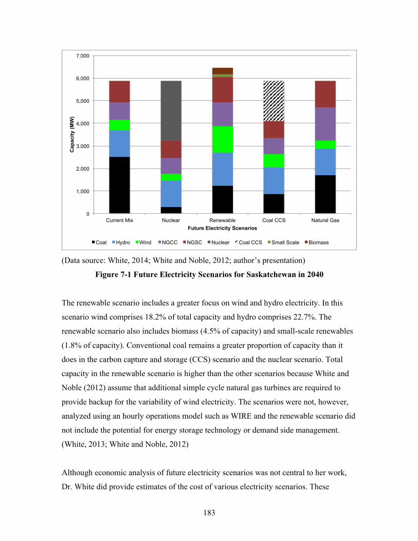
183

(Data source: White, 2014; White and Noble, 2012; author’s presentation)

Figure 7-1 Future Electricity Scenarios for Saskatchewan in 2040

The renewable scenario includes a greater focus on wind and hydro electricity. In this

scenario wind comprises 18.2% of total capacity and hydro comprises 22.7%. The

renewable scenario also includes biomass (4.5% of capacity) and small-scale renewables

(1.8% of capacity). Conventional coal remains a greater proportion of capacity than it

does in the carbon capture and storage (CCS) scenario and the nuclear scenario. Total

capacity in the renewable scenario is higher than the other scenarios because White and

Noble (2012) assume that additional simple cycle natural gas turbines are required to

provide backup for the variability of wind electricity. The scenarios were not, however,

analyzed using an hourly operations model such as WIRE and the renewable scenario did

not include the potential for energy storage technology or demand side management.

(White, 2013; White and Noble, 2012)

Although economic analysis of future electricity scenarios was not central to her work,

Dr. White did provide estimates of the cost of various electricity scenarios. These

0

1,000

2,000

3,000

4,000

5,000

6,000

7,000

Current Mix Nuclear Renewable Coal CCS Natural Gas

Cap

acity

(MW

)

Future Electricity Scenarios

Coal Hydro Wind NGCC NGSC Nuclear Coal CCS Small Scale Biomass

184

estimates were based on an estimate of the capital cost to build the facilities and an

estimate of the cost per kilowatt-hour to generate electricity. The costs are, however, a

simple weighted average of levelized cost estimates: they do not account for

technological progress and fuel price escalation; they do not address uncertainty; and they

are a static snapshot of expected prices in 2040, rather than a dynamic electricity price

pathway. Electricity prices and greenhouse gas emissions (GHGs) for the five scenarios

presented in White and Noble (2012) are summarized in Table 7-1. Despite the higher

financial cost for the renewable energy scenario, participants in the strategic

environmental assessment process indicated that this scenario was the preferred pathway

for the future of electricity in the province (White and Noble, 2012).

(Source: White and Noble, 2012)

Table 7-1 White and Noble (2012) Scenario Outcomes in 2040

In this chapter I present scenarios that are optimized to achieve environmental objectives

at the least financial cost to SaskPower. I also address the dynamics of improving

technology and increasing fuel prices, include a sensitivity analysis to address the

uncertainty inherent in estimates of future scenario costs, and use the WIRE model to test

whether the models can provide electricity on an hourly basis. I begin this analysis by

outlining SaskPower’s short- to medium-term electricity supply plan. This supply plan

informs my baseline business-as-usual scenario.

SaskPower’s Supply Plan

The baseline scenario in my analysis is designed to align with SaskPower’s stated

investment priorities. Knowledge of SaskPower’s supply plan out to 2030 is based on

interviews, SaskPower presentations, and news reports.

Current Mix Nuclear Renewable Coal CCS Natural GasGHG emissions (million tonnes CO2e/GWh) 19.6 7.3 11.5 8.0 15.7Cost of electricity ($/kWh) 0.11 0.12 0.14 0.13 0.10

185

The most important constraint faced by SaskPower is the Canadian federal government’s

coal-fired electricity regulation (CEPA, 2012). This regulation sets a maximum allowable

greenhouse-gas emission (GHG) intensity of 420 tonnes carbon dioxide (CO2) per

Gigawatt-hour (GWh) for coal-fired power plants. Existing Saskatchewan coal plants

must be either retired at the end of their useful life, or retrofitted with carbon capture and

storage (CCS) in order to comply with the regulation. Table 7-2 shows the retirement or

conversion schedule for Saskatchewan’s coal-fired electricity plants. If a commitment is

made to retrofit a given plant then it is allowed to operate as a conventional coal plant for

an additional five years before it must be equipped with CCS. The Boundary Dam III

carbon capture and storage (CCS) project was commissioned in 2014 and complies with

the federal regulation.

(Source: Interviews, 2014; CEPA, 2012)

Table 7-2 Saskatchewan Coal-fired Generation Regulatory Impact

As shown in Table 7-2, decisions must be made in the near future regarding Boundary

Dam units IV and V. Significant retirements are also scheduled in the period of 2028-

2030 when Boundary Dam VI and both units at Poplar River must be either retired or a

commitment made to convert them to CCS. Shand, which was commissioned in 1992, is

able to operate out to 2042, representing its fifty-year expected life.

Coal-fired UnitsCapacity

(MW) ComissionedRetirement If Not Converted to CCS

Conversion Deadline If

Converted to CCSBoundary Dam I 62 1959 RetiredBoundary Dam II 62 1959 RetiredBoundary Dam III 139/120 1970/2014 ConvertedBoundary Dam IV 139 1970 2019 2025Boundary Dam V 139 1973 2019 2025Boundary Dam VI 273 1978 2028 2033

Shand 279 1992 2042

Poplar River I 291 1981 2030Poplar River II 281 1983 2030

186

Environment Canada produced a Regulatory Impact Analysis Statement that accompanied

the coal-fired regulation (CEPA, 2012). This statement provides a cost-benefit analysis of

the impact of the regulation. Environment Canada modeled the impact using their in-

house E3MC energy-environment-economy model. In Saskatchewan they estimated the

coal-fired regulation would increase electricity generation costs by $1,174 million dollars

(present value 2010 $CDN) over the period of 2015 to 2035, and would increase average

electricity prices by 2.50 cents per kilowatt-hour (kWh) by 2035 (CEPA, 2012: 2064).

This is a greater price increase than that faced by Alberta (2.12 cents/kWh) and Nova

Scotia (1.40 cents/kWh). Part of the reason for the higher price impact is the choice of

how to comply with the regulation, “Saskatchewan officials indicated that the provincial

utility intends to implement CCS technology as a response to the regulatory performance

standard” (CEPA, 2012: 2018). As outlined in Chapter 5, coal-fired plants equipped with

CCS are expensive relative to other generation options. Saskatchewan officials like this

approach, however, because “Where the captured CO2 is used for enhanced oil recovery,

it generates additional benefits as a result of incremental oil production” (CEPA, 2012:

2018).65 The Saskatchewan government is also interested in maintaining employment in

the coal mining industry.

The baseline for my analysis assumes that Saskatchewan meets the regulatory

performance standard with a combination of conversion to CCS and retirement. I assume

that Boundary Dam units IV and V are retrofitted to CCS, allowing them to operate as

conventional plants until January 1st, 2025, when they begin to operate as CCS facilities.

I assume that Boundary Dam unit VI and both units at Poplar River are retired at the end

of their useful lives; they no longer operate as of 2030. I assume that the Shand coal plant

65 CEPA (2012) estimated that using captured CO2 for enhanced oil recovery could lead to $6 billion in additional oil extraction (valued at 2012 oil Western Texas Intermediate oil prices 2010 $CAN) between 2015 and 2035. Increases in emissions associated with EOR would total 5.4 Mt CO2e in that period, lowering GHG reductions created by the policy from 219.2 to 213.8 Mt Mt CO2e (CEPA, 2012).

187

is retrofitted in the 2025-2029 time-step to extend its life as a conventional coal plant

until the 2040-2044 time-step.66 Shand then operates as a CCS facility after 2045.

SaskPower’s baseline supply plan also includes investment in other technologies. The

following investments can be expected in the next fifteen years:

• Existing hydroelectric facilities will be repowered at the end of their scheduled

lives and retained as part of the electricity system;

• Investments will be made in wind capacity so that it composes 10% of capacity by

2020 and 20% by 2030. Note that this recent commitment by SaskPower means

that Saskatchewan will achieve the wind contribution outlined in White and

Noble’s (2012) renewable scenario within fifteen years;

• A small investment in biomass of 36-42 MW will be made at Meadow Lake;

• Small solar projects of 5-10 MW will be built to test the suitability of solar for the

Saskatchewan electricity system;

• SaskPower has signed a memorandum of understanding to purchase up to 500

MW of power from Manitoba Hydro. In September 2015 SaskPower signed an

agreement with Manitoba Hydro to secure 100 MW of power in the period 2020-

2040. I assume that SaskPower will purchase the additional 400 MW of

hydropower. This additional 400 MW of hydropower will enter service in the

period from 2020-2029;

• A 350 MW natural gas combined cycle plant will be built at Swift Current. More

investments in natural gas combined cycle and simple cycle will be made to make

up any shortfalls in electricity supply;

• SaskPower will pursue at least the lower potential of demand-side management

(DSM), but will also seek another 11 MW of peak savings.

Investment according to these assumptions creates an electricity system with 5869 MW

of capacity in 2025. After forcing these investments into the SIM model I optimize

investment decisions from 2030-2050. In this optimization I do not allow the construction

66 Environment Canada reports that a repowering of an existing coal plant can be assumed to cost $395/kilowatt (2012 $CDN) (CEPA, 2012: 2024).

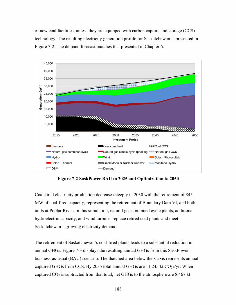
188

of new coal facilities, unless they are equipped with carbon capture and storage (CCS)

technology. The resulting electricity generation profile for Saskatchewan is presented in

Figure 7-2. The demand forecast matches that presented in Chapter 6.

Figure 7-2 SaskPower BAU to 2025 and Optimization to 2050

Coal-fired electricity production decreases steeply in 2030 with the retirement of 845

MW of coal-fired capacity, representing the retirement of Boundary Dam VI, and both

units at Poplar River. In this simulation, natural gas combined cycle plants, additional

hydroelectric capacity, and wind turbines replace retired coal plants and meet

Saskatchewan’s growing electricity demand.

The retirement of Saskatchewan’s coal-fired plants leads to a substantial reduction in

annual GHGs. Figure 7-3 displays the resulting annual GHGs from this SaskPower

business-as-usual (BAU) scenario. The thatched area below the x-axis represents annual

captured GHGs from CCS. By 2035 total annual GHGs are 11,245 kt CO2e/yr. When

captured CO2 is subtracted from that total, net GHGs to the atmosphere are 8,467 kt

-

5,000

10,000

15,000

20,000

25,000

30,000

35,000

40,000

45,000

2015 2020 2025 2030 2035 2040 2045 2050

Gen

erat

ion

(GW

h)

Investment Period

Biomass Coal compliant Coal CCS

Natural gas combined cycle Natural gas simple cycle (peaking) Natural gas CCS

Hydro Wind Solar - Photovoltaic

Solar - Thermal Small Modular Nuclear Reactor Manitoba Hydro

DSM Demand

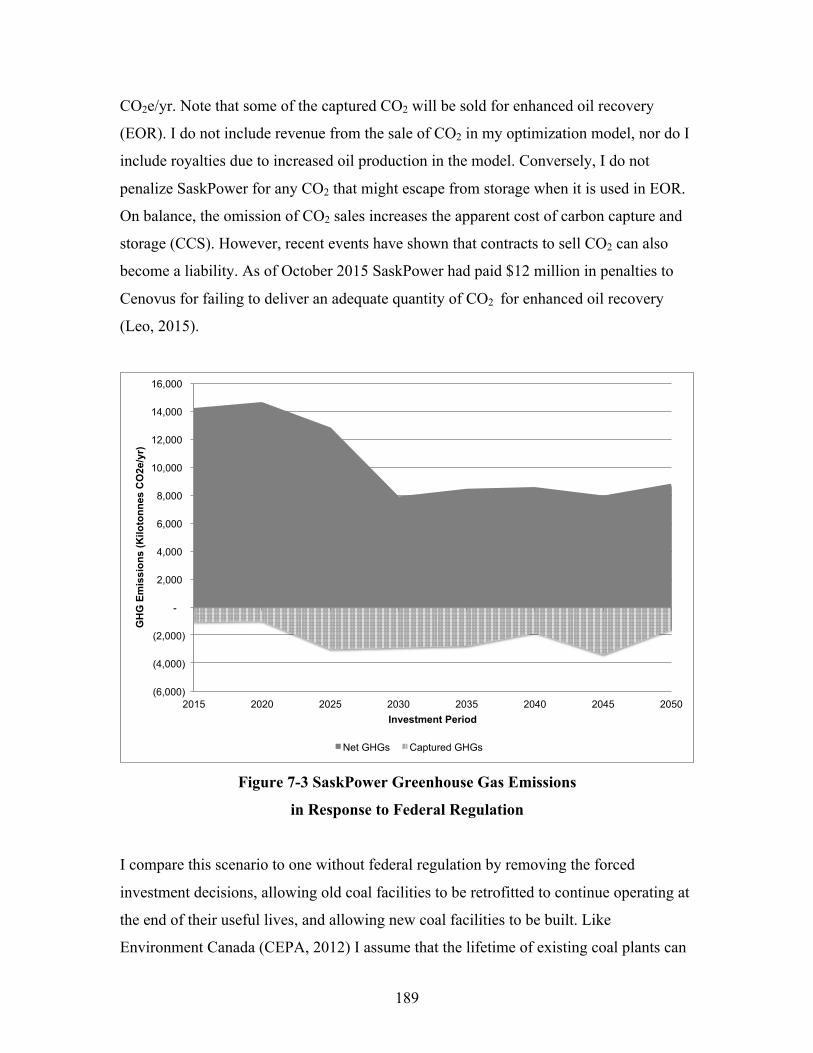
189

CO2e/yr. Note that some of the captured CO2 will be sold for enhanced oil recovery

(EOR). I do not include revenue from the sale of CO2 in my optimization model, nor do I

include royalties due to increased oil production in the model. Conversely, I do not

penalize SaskPower for any CO2 that might escape from storage when it is used in EOR.

On balance, the omission of CO2 sales increases the apparent cost of carbon capture and

storage (CCS). However, recent events have shown that contracts to sell CO2 can also

become a liability. As of October 2015 SaskPower had paid $12 million in penalties to

Cenovus for failing to deliver an adequate quantity of CO2 for enhanced oil recovery

(Leo, 2015).

Figure 7-3 SaskPower Greenhouse Gas Emissions

in Response to Federal Regulation

I compare this scenario to one without federal regulation by removing the forced

investment decisions, allowing old coal facilities to be retrofitted to continue operating at

the end of their useful lives, and allowing new coal facilities to be built. Like

Environment Canada (CEPA, 2012) I assume that the lifetime of existing coal plants can

(6,000)

(4,000)

(2,000)

-

2,000

4,000

6,000

8,000

10,000

12,000

14,000

16,000

2015 2020 2025 2030 2035 2040 2045 2050

GH

G E

mis

sion

s (K

iloto

nnes

CO

2e/y

r)

Investment Period

Net GHGs Captured GHGs

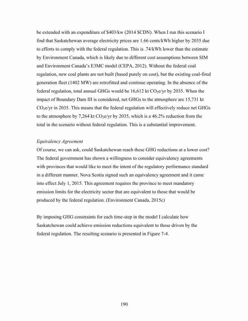
190

be extended with an expenditure of $403/kw (2014 $CDN). When I run this scenario I

find that Saskatchewan average electricity prices are 1.66 cents/kWh higher by 2035 due

to efforts to comply with the federal regulation. This is .74/kWh lower than the estimate

by Environment Canada, which is likely due to different cost assumptions between SIM

and Environment Canada’s E3MC model (CEPA, 2012). Without the federal coal

regulation, new coal plants are not built (based purely on cost), but the existing coal-fired

generation fleet (1402 MW) are retrofitted and continue operating. In the absence of the

federal regulation, total annual GHGs would be 16,612 kt CO2e/yr by 2035. When the

impact of Boundary Dam III is considered, net GHGs to the atmosphere are 15,731 kt

CO2e/yr in 2035. This means that the federal regulation will effectively reduce net GHGs

to the atmosphere by 7,264 kt CO2e/yr by 2035, which is a 46.2% reduction from the

total in the scenario without federal regulation. This is a substantial improvement.

Equivalency Agreement

Of course, we can ask, could Saskatchewan reach these GHG reductions at a lower cost?

The federal government has shown a willingness to consider equivalency agreements

with provinces that would like to meet the intent of the regulatory performance standard

in a different manner. Nova Scotia signed such an equivalency agreement and it came

into effect July 1, 2015. This agreement requires the province to meet mandatory

emission limits for the electricity sector that are equivalent to those that would be

produced by the federal regulation. (Environment Canada, 2015c)

By imposing GHG constraints for each time-step in the model I calculate how

Saskatchewan could achieve emission reductions equivalent to those driven by the

federal regulation. The resulting scenario is presented in Figure 7-4.

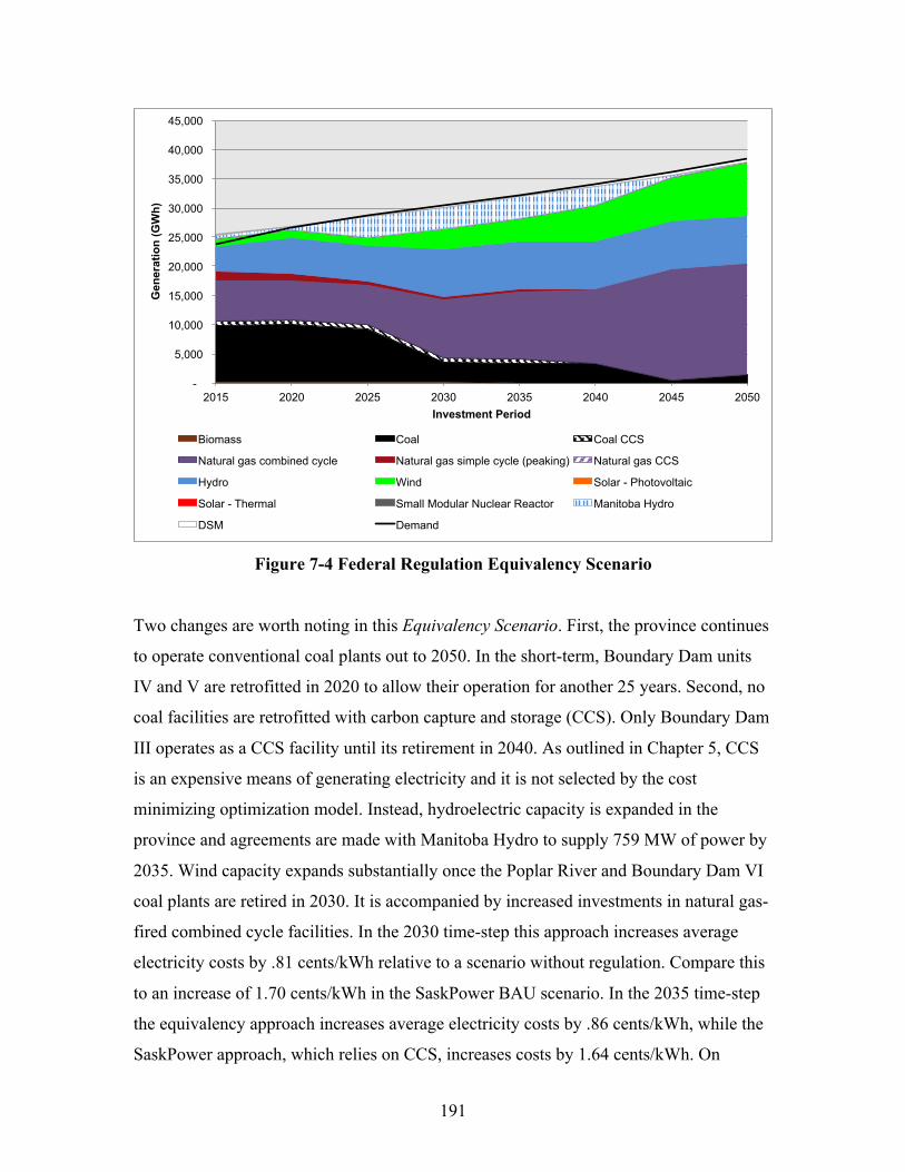
191

Figure 7-4 Federal Regulation Equivalency Scenario

Two changes are worth noting in this Equivalency Scenario. First, the province continues

to operate conventional coal plants out to 2050. In the short-term, Boundary Dam units

IV and V are retrofitted in 2020 to allow their operation for another 25 years. Second, no

coal facilities are retrofitted with carbon capture and storage (CCS). Only Boundary Dam

III operates as a CCS facility until its retirement in 2040. As outlined in Chapter 5, CCS

is an expensive means of generating electricity and it is not selected by the cost

minimizing optimization model. Instead, hydroelectric capacity is expanded in the

province and agreements are made with Manitoba Hydro to supply 759 MW of power by

2035. Wind capacity expands substantially once the Poplar River and Boundary Dam VI

coal plants are retired in 2030. It is accompanied by increased investments in natural gas-

fired combined cycle facilities. In the 2030 time-step this approach increases average

electricity costs by .81 cents/kWh relative to a scenario without regulation. Compare this

to an increase of 1.70 cents/kWh in the SaskPower BAU scenario. In the 2035 time-step

the equivalency approach increases average electricity costs by .86 cents/kWh, while the

SaskPower approach, which relies on CCS, increases costs by 1.64 cents/kWh. On

-

5,000

10,000

15,000

20,000

25,000

30,000

35,000

40,000

45,000

2015 2020 2025 2030 2035 2040 2045 2050

Gen

erat

ion

(GW

h)

Investment Period

Biomass Coal Coal CCS

Natural gas combined cycle Natural gas simple cycle (peaking) Natural gas CCS

Hydro Wind Solar - Photovoltaic

Solar - Thermal Small Modular Nuclear Reactor Manitoba Hydro

DSM Demand

192

average from 2030-2050 the equivalency approach saves .86 cents/kWh relative to the

SaskPower approach.

Figure 7-5 compares the pathway of average electricity prices under the three scenarios:

SaskPower’s BAU response to federal regulations; an equivalency approach to achieving

the same GHG reductions; and a scenario where no policy is enacted to limit GHGs. The

expected average prices for each scenario are joined by the solid lines. The 5% and 95%

confidence intervals are represented using the error bars that surround each price point.

Note that the confidence intervals for the equivalency scenario overlap with the no-policy

scenario in several time-steps.

Figure 7-5 Average Electricity Prices Comparing Federal Regulation to Equivalency

The confidence intervals in Figure 7-5 reflect three sources of uncertainty:

1. The rate at which capital costs will change for electricity generation technologies;

2. The rate at which power purchased from Manitoba Hydro will increase in price;

0.0

1.0

2.0

3.0

4.0

5.0

6.0

7.0

8.0

9.0

10.0

11.0

12.0

13.0

14.0

15.0

16.0

2015 2020 2025 2030 2035 2040 2045 2050

Ave

rage

Cos

t of E

lect

rici

ty (c

ents

/kW

h) (2

014

$C

AN

)

Time Step

SaskPower BAU BAU Equivalent No GHG Policy

193

3. The future price of natural gas.

A Monte Carlo analysis was conducted allowing each of these factors to vary within a

specified range. Due to lack of data, a Triangular distribution was chosen for each

uncertain parameter. The distributions were bounded in the following manner:

1. The autonomous capital cost improvement (ACCI) parameter for each electricity

generation technology was bounded by .5% on either side of the preset value.

The only exception is nuclear, which has a likely value of 1.54% (the preset

value derived from EIA, 2015), and which is bounded by 2.04% on the high side

and 0% on the low side. This lower bound for cost improvement is based on

historic difficulties achieving cost reductions (Grubler, 2010; Boccard, 2014);

2. The likely cost escalation factor for Manitoba Hydro power was set at 1% and

was bounded by a .5% minimum and a 1.5% maximum;

3. The NEB (2013) reference price is set as the most likely price of natural gas, and

the distribution is bounded by the high and low NEB (2013) forecast natural gas

prices for each time period.

Using these distributions I ran 1000 Monte Carlo trials using Frontline Solver’s ‘Risk

Solver Pro’ software. The results from these simulations were used to create the

confidence intervals in Figures 7-5, 7-11, 7-18, and 7-22.

Long-Term GHG Reduction

The federal coal-fired regulations achieve a nearly fifty-percent reduction of

Saskatchewan’s electricity sector GHGs by 2035 followed by no further reduction to

2045. This is a substantial improvement, but as Figure 7-3 indicates, GHG emissions in

the electricity sector begin to increase after 2045 as natural gas combined cycle plants

expand to meet growing demand.

Further reductions are required if the province is to contribute to global efforts to mitigate

climate change. In their Fifth Assessment Report, the IPCC (2014) outlines several

scenarios for our future climate. In scenarios where it is likely (although not certain) that

194

average temperature change will remain below two degrees Celsius relative to pre-

industrial levels, atmospheric concentrations of GHGs lie in the realm of 450 ppm CO2e

by 2100. To achieve these scenarios, and stabilize atmospheric concentrations at or below

450 ppm CO2e, global GHG emissions must be near zero by 2100. This requires a

significant transformation of our energy systems. Low-carbon energy must compose over

90% of primary energy by 2100 and substantial gains need to be made by 2050. (IPCC,

2014)

Saskatchewan once had a provincial target of reducing GHGs to 80% below 2004 levels

by 2050. This target was first proposed by the NDP government, and was upheld by the

Saskatchewan Party government in their first term. The Saskatchewan government has

since backed away from the 2050 target and instead current legislation reads, “The

Lieutenant Governor in Council shall establish a greenhouse gas emission reduction

target for Saskatchewan for a year or years selected by the Lieutenant Governor in

Council” (Government of Saskatchewan, 2015). A new GHG reduction target has not

been set at the time of writing this dissertation.

GHGs from the ‘public electricity and heat production’ sector in Saskatchewan measured

16,705 kt CO2e in 2004 and decreased to 16,010 kt CO2e by 2013 (Environment Canada,

2015b). In the scenario below, I use SIM to solve for the least-cost pathway to achieve an

80% reduction in GHGs by 2050 relative to 2015 levels. There are three variations of this

scenario; one allowing imports of hydroelectricity from Manitoba of up to 1950 MW,

another relying on electricity produced in Saskatchewan alone, and a third that excludes

both nuclear power and increased imports from Manitoba Hydro. All of the scenarios

include the 100 MW that Manitoba Hydro has already agreed to provide to SaskPower

between 2020 and 2040. As a caveat, I focus only on direct GHG emissions and not the

life-cycle GHG emissions related to each technology. More work could be done to

understand the full lifecycle GHG implications of each electricity scenario.

80% GHG Reduction: Scenario 1 – Interprovincial approach

To generate the first 80% GHG reduction scenario, I run SIM using all available

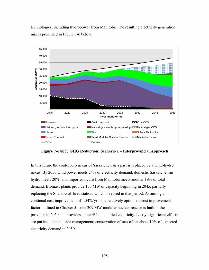
195

technologies, including hydropower from Manitoba. The resulting electricity generation

mix is presented in Figure 7-6 below.

Figure 7-6 80% GHG Reduction: Scenario 1 – Interprovincial Approach

In this future the coal-hydro nexus of Saskatchewan’s past is replaced by a wind-hydro

nexus. By 2050 wind power meets 24% of electricity demand, domestic Saskatchewan

hydro meets 20%, and imported hydro from Manitoba meets another 19% of total

demand. Biomass plants provide 150 MW of capacity beginning in 2045, partially

replacing the Shand coal-fired station, which is retired in that period. Assuming a

continual cost improvement of 1.54%/yr – the relatively optimistic cost improvement

factor outlined in Chapter 5 – one 209 MW modular nuclear reactor is built in the

province in 2050 and provides about 4% of supplied electricity. Lastly, significant efforts

are put into demand side management; conservation efforts offset about 10% of expected

electricity demand in 2050.

-

5,000

10,000

15,000

20,000

25,000

30,000

35,000

40,000

45,000

2015 2020 2025 2030 2035 2040 2045 2050

Gen

erat

ion

(GW

h)

Investment Period

Biomass Coal compliant Coal CCS

Natural gas combined cycle Natural gas simple cycle (peaking) Natural gas CCS

Hydro Wind Solar - Photovoltaic

Solar - Thermal Small Modular Nuclear Reactor Manitoba Hydro

DSM Demand

196

Note that in this scenario coal plants are retired at the end of their useful lives; options to

retrofit existing coal plants are excluded except for the Shand station which continues to

operate until 2045. As well, the amount of electricity that can be generated by wind is

constrained to 6% in 2020, which corresponds to SaskPower’s commitment that wind

will compose 10% of capacity by that time. Allowable wind generated electricity then

increases by 3% in every time step; in 2030 12% of electricity can be generated by wind,

corresponding to SaskPower’s commitment that wind will compose 20% of capacity by

that time; in 2050 24% of electricity can be generated by wind. This assumes that

SaskPower will gain experience integrating wind into the electricity system. This is a

broadly accepted assumption; most of the experts that took part in the participatory

modelling workshops believed that variable renewables like wind and solar could

contribute at least 24% to the Saskatchewan electricity system by 2050.

I use the WIRE model to test whether this scenario could sufficiently meet electricity

demand in four representative months: March, June, September and December. The

resulting system operation in December of 2050 is displayed in Figure 7-7. The jagged

green portion of the image shows the variable contribution of the 2800 MW of wind.

Along the bottom, the biomass plants (brown) provide a steady supply of power. The

purple bar above shows natural gas combined cycle plants reacting to variations in wind

power. Domestic hydroelectric power (light blue) also acts as a balancing technology and

ramps up to provide power when wind power drops off. Imports from Manitoba Hydro

fill the remaining gap. Because it is December, a period of reduced stream flows, the

capacity factors for both domestic and Manitoba hydropower production are constrained

to 48% in the WIRE model; the domestic hydro plants achieve this capacity factor, while

the 1950 MW Manitoba Hydro link operates at only a 30% capacity factor. The Manitoba

Hydro link does provide a peak supply of 1367 MW in hour 523 when wind power

production falls to 22 MW. As outlined in Appendix 7B, I assume that the hydroelectric

facilities can ramp up to full capacity within an hour and that hydroelectric potential can

be stored in reservoirs when not needed.

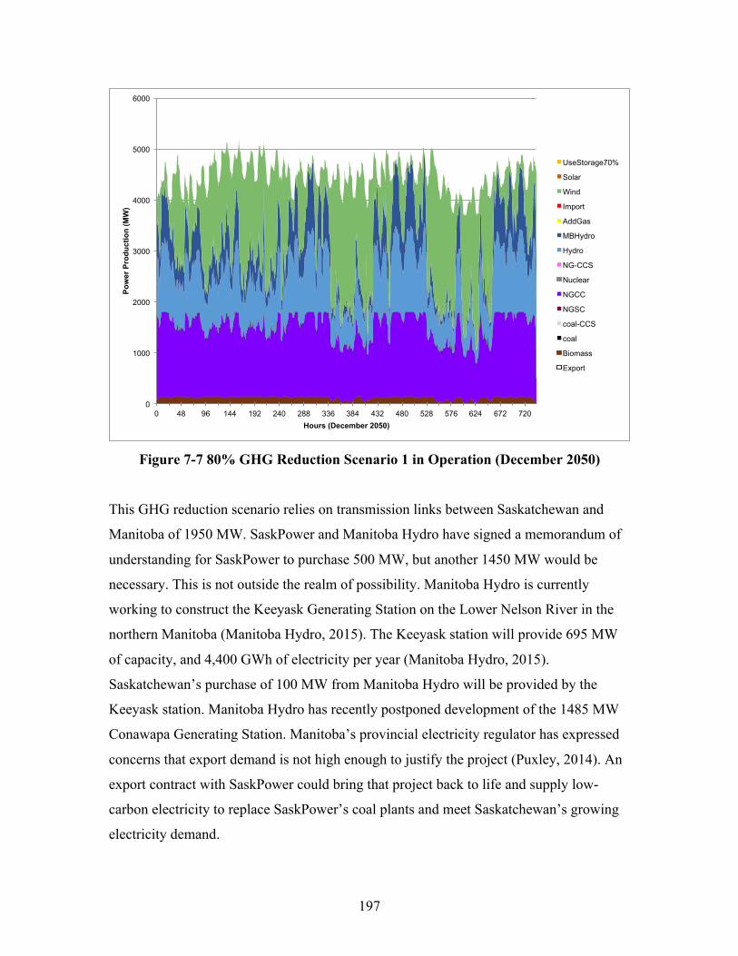
197

Figure 7-7 80% GHG Reduction Scenario 1 in Operation (December 2050)

This GHG reduction scenario relies on transmission links between Saskatchewan and

Manitoba of 1950 MW. SaskPower and Manitoba Hydro have signed a memorandum of

understanding for SaskPower to purchase 500 MW, but another 1450 MW would be

necessary. This is not outside the realm of possibility. Manitoba Hydro is currently

working to construct the Keeyask Generating Station on the Lower Nelson River in the

northern Manitoba (Manitoba Hydro, 2015). The Keeyask station will provide 695 MW

of capacity, and 4,400 GWh of electricity per year (Manitoba Hydro, 2015).

Saskatchewan’s purchase of 100 MW from Manitoba Hydro will be provided by the

Keeyask station. Manitoba Hydro has recently postponed development of the 1485 MW

Conawapa Generating Station. Manitoba’s provincial electricity regulator has expressed

concerns that export demand is not high enough to justify the project (Puxley, 2014). An

export contract with SaskPower could bring that project back to life and supply low-

carbon electricity to replace SaskPower’s coal plants and meet Saskatchewan’s growing

electricity demand.

0

1000

2000

3000

4000

5000

6000

0 48 96 144 192 240 288 336 384 432 480 528 576 624 672 720

Pow

er P

rodu

ctio

n (M

W)

Hours (December 2050)

UseStorage70%

Solar

Wind

Import

AddGas

MBHydro

Hydro

NG-CCS

Nuclear

NGCC

NGSC

coal-CCS

coal

Biomass

Export

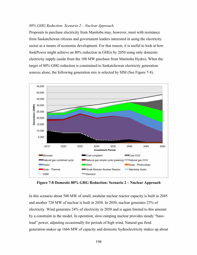
198

80% GHG Reduction: Scenario 2 – Nuclear Approach

Proposals to purchase electricity from Manitoba may, however, meet with resistance

from Saskatchewan citizens and government leaders interested in using the electricity

sector as a means of economic development. For that reason, it is useful to look at how

SaskPower might achieve an 80% reduction in GHGs by 2050 using only domestic

electricity supply (aside from the 100 MW purchase from Manitoba Hydro). When the

target of 80% GHG reduction is constrained to Saskatchewan electricity generation

sources alone, the following generation mix is selected by SIM (See Figure 7-8).

Figure 7-8 Domestic 80% GHG Reduction: Scenario 2 – Nuclear Approach

In this scenario about 500 MW of small, modular nuclear reactor capacity is built in 2045

and another 720 MW of nuclear is built in 2050. In 2050, nuclear generates 23% of

electricity. Wind generates 24% of electricity in 2050 and is again limited to this amount

by a constraint in the model. In operation, slow-ramping nuclear provides steady “base-

load” power, adjusting occasionally for periods of high wind. Natural-gas fired

generation makes up 1666 MW of capacity and domestic hydroelectricity makes up about

-

5,000

10,000

15,000

20,000

25,000

30,000

35,000

40,000

45,000

2015 2020 2025 2030 2035 2040 2045 2050

Gen

erat

ion

(GW

h)

Investment Period

Biomass Coal compliant Coal CCS

Natural gas combined cycle Natural gas simple cycle (peaking) Natural gas CCS

Hydro Wind Solar - Photovoltaic

Solar - Thermal Small Modular Nuclear Reactor Manitoba Hydro

DSM Demand

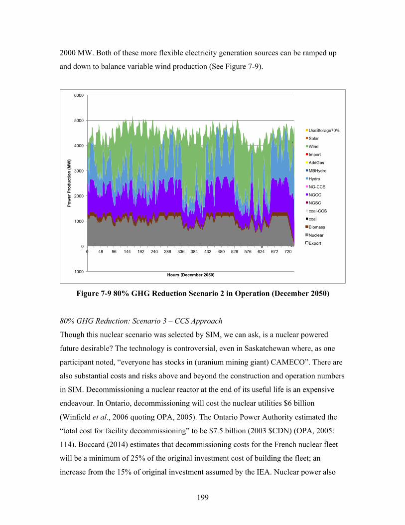
199

2000 MW. Both of these more flexible electricity generation sources can be ramped up

and down to balance variable wind production (See Figure 7-9).

Figure 7-9 80% GHG Reduction Scenario 2 in Operation (December 2050)

80% GHG Reduction: Scenario 3 – CCS Approach

Though this nuclear scenario was selected by SIM, we can ask, is a nuclear powered

future desirable? The technology is controversial, even in Saskatchewan where, as one

participant noted, “everyone has stocks in (uranium mining giant) CAMECO”. There are

also substantial costs and risks above and beyond the construction and operation numbers

in SIM. Decommissioning a nuclear reactor at the end of its useful life is an expensive

endeavour. In Ontario, decommissioning will cost the nuclear utilities $6 billion

(Winfield et al., 2006 quoting OPA, 2005). The Ontario Power Authority estimated the

“total cost for facility decommissioning” to be $7.5 billion (2003 $CDN) (OPA, 2005:

114). Boccard (2014) estimates that decommissioning costs for the French nuclear fleet

will be a minimum of 25% of the original investment cost of building the fleet; an

increase from the 15% of original investment assumed by the IEA. Nuclear power also

-1000

0

1000

2000

3000

4000

5000

6000

0 48 96 144 192 240 288 336 384 432 480 528 576 624 672 720

Pow

er P

rodu

ctio

n (M

W)

Hours (December 2050)

UseStorage70%

Solar

Wind

Import

AddGas

MBHydro

Hydro

NG-CCS

NGCC

NGSC

coal-CCS

coal

Biomass

Nuclear

Export

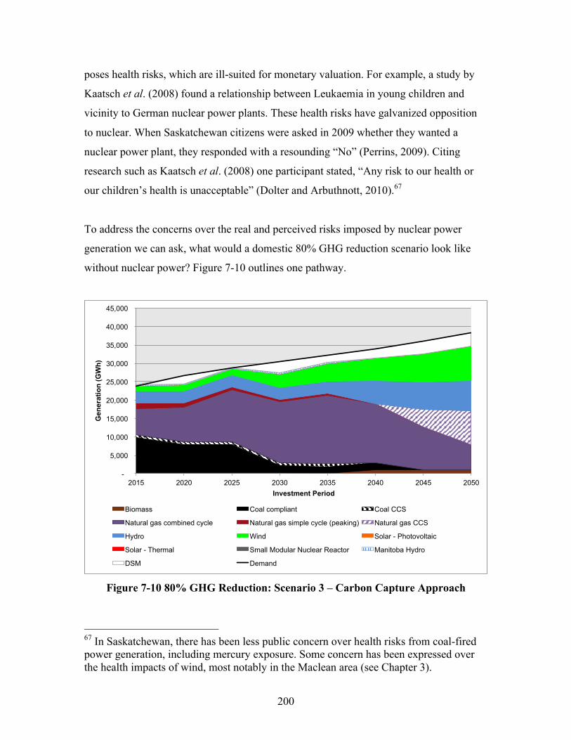
200

poses health risks, which are ill-suited for monetary valuation. For example, a study by

Kaatsch et al. (2008) found a relationship between Leukaemia in young children and

vicinity to German nuclear power plants. These health risks have galvanized opposition

to nuclear. When Saskatchewan citizens were asked in 2009 whether they wanted a

nuclear power plant, they responded with a resounding “No” (Perrins, 2009). Citing

research such as Kaatsch et al. (2008) one participant stated, “Any risk to our health or

our children’s health is unacceptable” (Dolter and Arbuthnott, 2010).67

To address the concerns over the real and perceived risks imposed by nuclear power

generation we can ask, what would a domestic 80% GHG reduction scenario look like

without nuclear power? Figure 7-10 outlines one pathway.

Figure 7-10 80% GHG Reduction: Scenario 3 – Carbon Capture Approach

67 In Saskatchewan, there has been less public concern over health risks from coal-fired power generation, including mercury exposure. Some concern has been expressed over the health impacts of wind, most notably in the Maclean area (see Chapter 3).

-

5,000

10,000

15,000

20,000

25,000

30,000

35,000

40,000

45,000

2015 2020 2025 2030 2035 2040 2045 2050

Gen

erat

ion

(GW

h)

Investment Period

Biomass Coal compliant Coal CCS

Natural gas combined cycle Natural gas simple cycle (peaking) Natural gas CCS

Hydro Wind Solar - Photovoltaic

Solar - Thermal Small Modular Nuclear Reactor Manitoba Hydro

DSM Demand

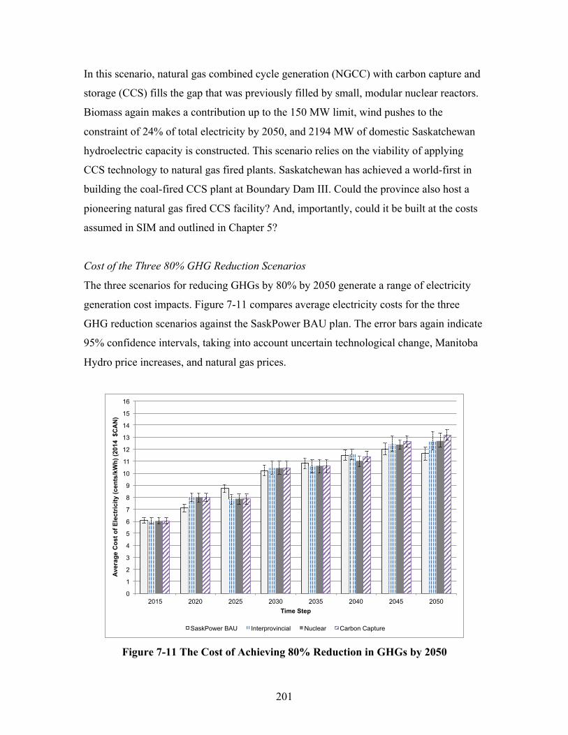
201

In this scenario, natural gas combined cycle generation (NGCC) with carbon capture and

storage (CCS) fills the gap that was previously filled by small, modular nuclear reactors.

Biomass again makes a contribution up to the 150 MW limit, wind pushes to the

constraint of 24% of total electricity by 2050, and 2194 MW of domestic Saskatchewan

hydroelectric capacity is constructed. This scenario relies on the viability of applying

CCS technology to natural gas fired plants. Saskatchewan has achieved a world-first in

building the coal-fired CCS plant at Boundary Dam III. Could the province also host a

pioneering natural gas fired CCS facility? And, importantly, could it be built at the costs

assumed in SIM and outlined in Chapter 5?

Cost of the Three 80% GHG Reduction Scenarios

The three scenarios for reducing GHGs by 80% by 2050 generate a range of electricity

generation cost impacts. Figure 7-11 compares average electricity costs for the three

GHG reduction scenarios against the SaskPower BAU plan. The error bars again indicate

95% confidence intervals, taking into account uncertain technological change, Manitoba

Hydro price increases, and natural gas prices.

Figure 7-11 The Cost of Achieving 80% Reduction in GHGs by 2050

0

1

2

3

4

5

6

7

8

9

10

11

12

13

14

15

16

2015 2020 2025 2030 2035 2040 2045 2050

Ave

rage

Cos

t of E

lect

rici

ty (c

ents

/kW

h) (2

014

$C

AN

)

Time Step

SaskPower BAU Interprovincial Nuclear Carbon Capture

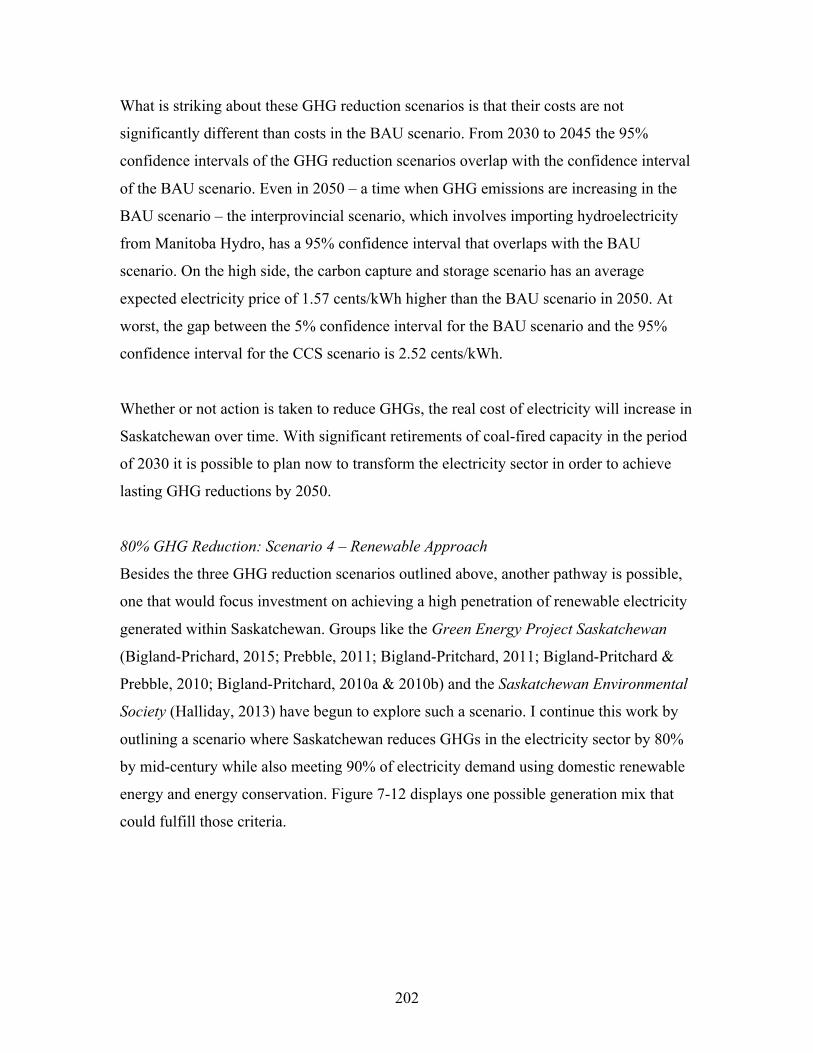
202

What is striking about these GHG reduction scenarios is that their costs are not

significantly different than costs in the BAU scenario. From 2030 to 2045 the 95%

confidence intervals of the GHG reduction scenarios overlap with the confidence interval

of the BAU scenario. Even in 2050 – a time when GHG emissions are increasing in the

BAU scenario – the interprovincial scenario, which involves importing hydroelectricity

from Manitoba Hydro, has a 95% confidence interval that overlaps with the BAU

scenario. On the high side, the carbon capture and storage scenario has an average

expected electricity price of 1.57 cents/kWh higher than the BAU scenario in 2050. At

worst, the gap between the 5% confidence interval for the BAU scenario and the 95%

confidence interval for the CCS scenario is 2.52 cents/kWh.

Whether or not action is taken to reduce GHGs, the real cost of electricity will increase in

Saskatchewan over time. With significant retirements of coal-fired capacity in the period

of 2030 it is possible to plan now to transform the electricity sector in order to achieve

lasting GHG reductions by 2050.

80% GHG Reduction: Scenario 4 – Renewable Approach

Besides the three GHG reduction scenarios outlined above, another pathway is possible,

one that would focus investment on achieving a high penetration of renewable electricity

generated within Saskatchewan. Groups like the Green Energy Project Saskatchewan

(Bigland-Prichard, 2015; Prebble, 2011; Bigland-Pritchard, 2011; Bigland-Pritchard &

Prebble, 2010; Bigland-Pritchard, 2010a & 2010b) and the Saskatchewan Environmental

Society (Halliday, 2013) have begun to explore such a scenario. I continue this work by

outlining a scenario where Saskatchewan reduces GHGs in the electricity sector by 80%

by mid-century while also meeting 90% of electricity demand using domestic renewable

energy and energy conservation. Figure 7-12 displays one possible generation mix that

could fulfill those criteria.

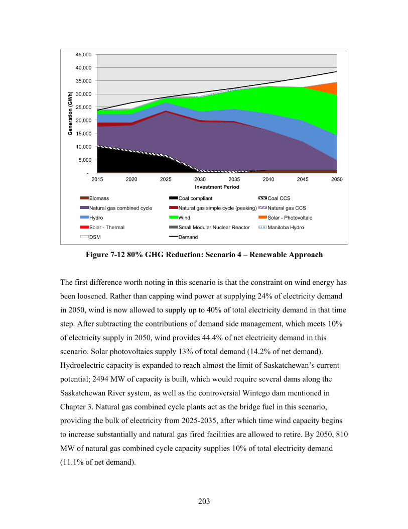
203

Figure 7-12 80% GHG Reduction: Scenario 4 – Renewable Approach

The first difference worth noting in this scenario is that the constraint on wind energy has

been loosened. Rather than capping wind power at supplying 24% of electricity demand

in 2050, wind is now allowed to supply up to 40% of total electricity demand in that time

step. After subtracting the contributions of demand side management, which meets 10%

of electricity supply in 2050, wind provides 44.4% of net electricity demand in this

scenario. Solar photovoltaics supply 13% of total demand (14.2% of net demand).

Hydroelectric capacity is expanded to reach almost the limit of Saskatchewan’s current

potential; 2494 MW of capacity is built, which would require several dams along the

Saskatchewan River system, as well as the controversial Wintego dam mentioned in

Chapter 3. Natural gas combined cycle plants act as the bridge fuel in this scenario,

providing the bulk of electricity from 2025-2035, after which time wind capacity begins

to increase substantially and natural gas fired facilities are allowed to retire. By 2050, 810

MW of natural gas combined cycle capacity supplies 10% of total electricity demand

(11.1% of net demand).

-

5,000

10,000

15,000

20,000

25,000

30,000

35,000

40,000

45,000

2015 2020 2025 2030 2035 2040 2045 2050

Gen

erat

ion

(GW

h)

Investment Period

Biomass Coal compliant Coal CCS

Natural gas combined cycle Natural gas simple cycle (peaking) Natural gas CCS

Hydro Wind Solar - Photovoltaic

Solar - Thermal Small Modular Nuclear Reactor Manitoba Hydro

DSM Demand

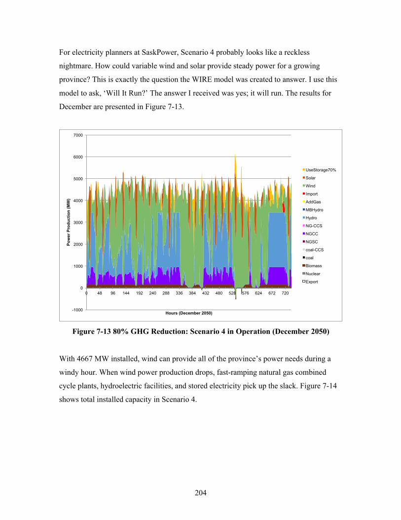
204

For electricity planners at SaskPower, Scenario 4 probably looks like a reckless

nightmare. How could variable wind and solar provide steady power for a growing

province? This is exactly the question the WIRE model was created to answer. I use this

model to ask, ‘Will It Run?’ The answer I received was yes; it will run. The results for

December are presented in Figure 7-13.

Figure 7-13 80% GHG Reduction: Scenario 4 in Operation (December 2050)

With 4667 MW installed, wind can provide all of the province’s power needs during a

windy hour. When wind power production drops, fast-ramping natural gas combined

cycle plants, hydroelectric facilities, and stored electricity pick up the slack. Figure 7-14

shows total installed capacity in Scenario 4.

-1000

0

1000

2000

3000

4000

5000

6000

7000

0 48 96 144 192 240 288 336 384 432 480 528 576 624 672 720

Pow

er P

rodu

ctio

n (M

W)

Hours (December 2050)

UseStorage70%

Solar

Wind

Import

AddGas

MBHydro

Hydro

NG-CCS

NGCC

NGSC

coal-CCS

coal

Biomass

Nuclear

Export

205

Figure 7-14 Electricity Capacity in Domestic Renewable Energy Scenario

In this scenario storage capacity plays an increasingly important role towards the end of

the investment period (see teal blue wedge in Figure 7-14). By 2050 this scenario

includes about 6500 MW of electricity storage capacity. This storage capacity is

recharged in periods when sun and wind are abundant, and drawn down when it is cloudy

and calm. The yellow bits at the peaks in Figure 7-13 (previous page) indicate when

electricity storage is drawn upon. As can be seen, the stored energy becomes important in

the latter part of the month when natural gas combined cycle plants and hydroelectric

facilities are operating at full capacity and further energy is needed to meet demand. On

an hourly basis storage capacity helps to smooth out the contribution of wind and solar

energy. Storage capacity also adds to the cost of the electricity system.

Grid integration of wind and solar is aided by the demand side management (DSM)

strategy of peak shifting. In this scenario 370 MW of peak shaving is allowed. I model

this in WIRE by allowing electricity demand to be shifted three hours into the future (see

Appendix 7B for further detail). This is introduced with the constraint,

-

5,000

10,000

15,000

20,000

25,000

2015 2020 2025 2030 2035 2040 2045 2050

Cap

acity

(MW

)

Investment Period

Biomass Coal Coal CCS

Natural gas combined cycle Natural gas simple cycle (peaking) Natural gas CCS

Hydro Wind Solar - Photovoltaic

Solar - Thermal Small Modular Nuclear Reactor Manitoba Hydro

DSM Peak Savings Storage

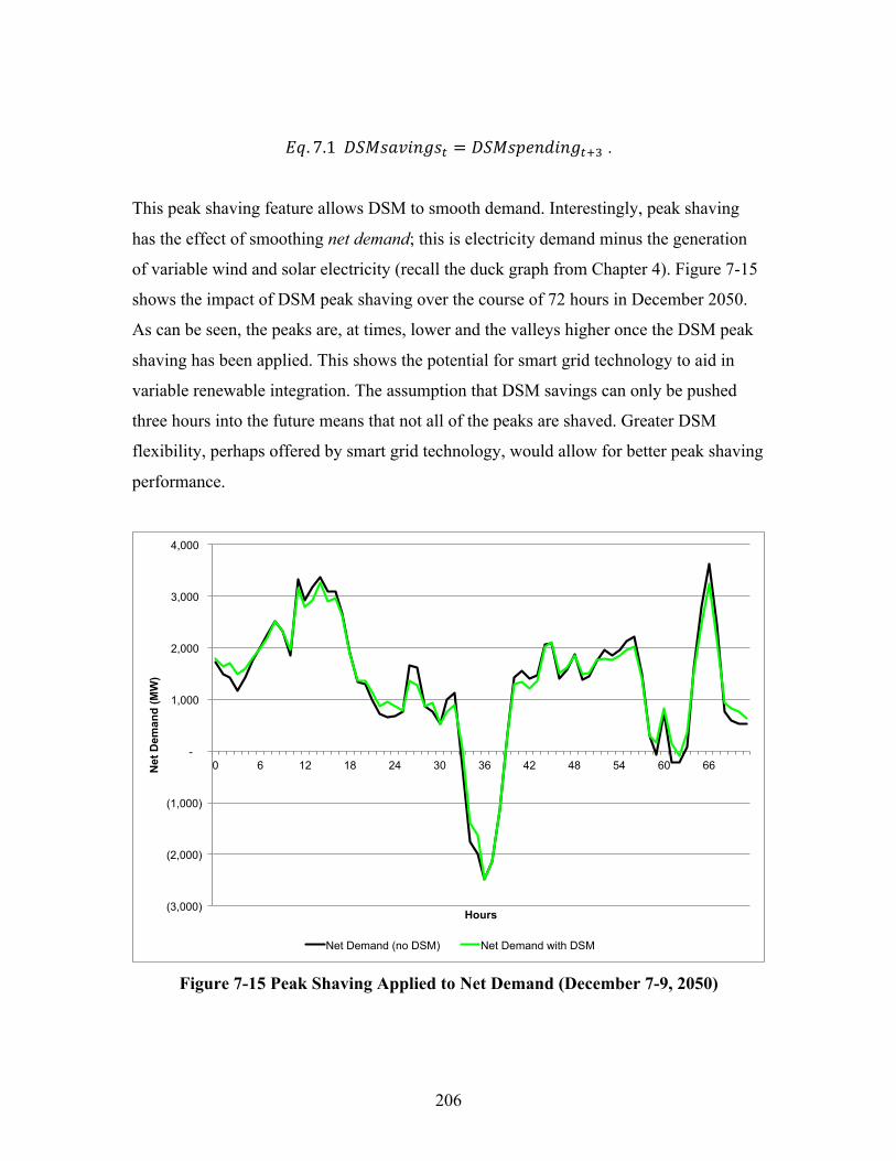
206

𝐸𝑞. 7.1 𝐷𝑆𝑀𝑠𝑎𝑣𝑖𝑛𝑔𝑠! = 𝐷𝑆𝑀𝑠𝑝𝑒𝑛𝑑𝑖𝑛𝑔!!! .

This peak shaving feature allows DSM to smooth demand. Interestingly, peak shaving

has the effect of smoothing net demand; this is electricity demand minus the generation

of variable wind and solar electricity (recall the duck graph from Chapter 4). Figure 7-15

shows the impact of DSM peak shaving over the course of 72 hours in December 2050.

As can be seen, the peaks are, at times, lower and the valleys higher once the DSM peak

shaving has been applied. This shows the potential for smart grid technology to aid in

variable renewable integration. The assumption that DSM savings can only be pushed

three hours into the future means that not all of the peaks are shaved. Greater DSM

flexibility, perhaps offered by smart grid technology, would allow for better peak shaving

performance.

Figure 7-15 Peak Shaving Applied to Net Demand (December 7-9, 2050)

(3,000)

(2,000)

(1,000)

-

1,000

2,000

3,000

4,000

0 6 12 18 24 30 36 42 48 54 60 66 Net

Dem

and

(MW

)

Hours

Net Demand (no DSM) Net Demand with DSM

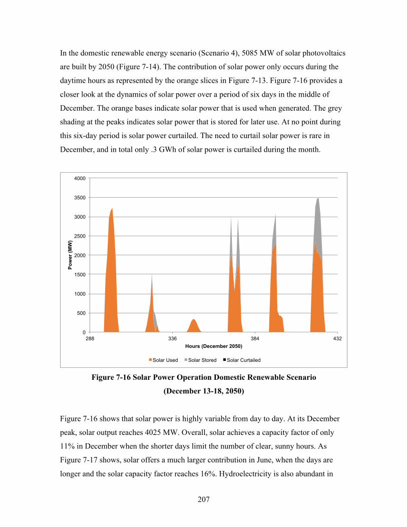
207

In the domestic renewable energy scenario (Scenario 4), 5085 MW of solar photovoltaics

are built by 2050 (Figure 7-14). The contribution of solar power only occurs during the

daytime hours as represented by the orange slices in Figure 7-13. Figure 7-16 provides a

closer look at the dynamics of solar power over a period of six days in the middle of

December. The orange bases indicate solar power that is used when generated. The grey

shading at the peaks indicates solar power that is stored for later use. At no point during

this six-day period is solar power curtailed. The need to curtail solar power is rare in

December, and in total only .3 GWh of solar power is curtailed during the month.

Figure 7-16 Solar Power Operation Domestic Renewable Scenario

(December 13-18, 2050)

Figure 7-16 shows that solar power is highly variable from day to day. At its December

peak, solar output reaches 4025 MW. Overall, solar achieves a capacity factor of only

11% in December when the shorter days limit the number of clear, sunny hours. As

Figure 7-17 shows, solar offers a much larger contribution in June, when the days are

longer and the solar capacity factor reaches 16%. Hydroelectricity is also abundant in

0

500

1000

1500

2000

2500

3000

3500

4000

288 336 384 432

Pow

er (M

W)

Hours (December 2050)

Solar Used Solar Stored Solar Curtailed

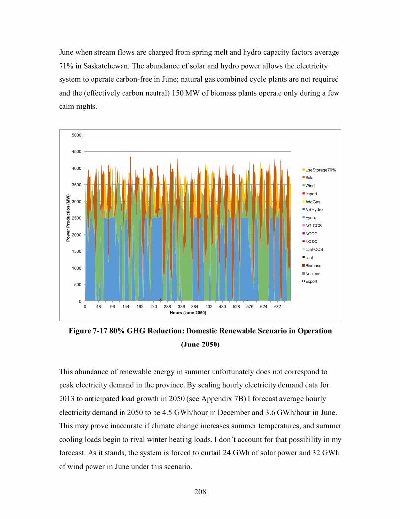
208

June when stream flows are charged from spring melt and hydro capacity factors average

71% in Saskatchewan. The abundance of solar and hydro power allows the electricity

system to operate carbon-free in June; natural gas combined cycle plants are not required

and the (effectively carbon neutral) 150 MW of biomass plants operate only during a few

calm nights.

Figure 7-17 80% GHG Reduction: Domestic Renewable Scenario in Operation

(June 2050)

This abundance of renewable energy in summer unfortunately does not correspond to

peak electricity demand in the province. By scaling hourly electricity demand data for

2013 to anticipated load growth in 2050 (see Appendix 7B) I forecast average hourly

electricity demand in 2050 to be 4.5 GWh/hour in December and 3.6 GWh/hour in June.

This may prove inaccurate if climate change increases summer temperatures, and summer

cooling loads begin to rival winter heating loads. I don’t account for that possibility in my

forecast. As it stands, the system is forced to curtail 24 GWh of solar power and 32 GWh

of wind power in June under this scenario.

0

500

1000

1500

2000

2500

3000

3500

4000

4500

5000

0 48 96 144 192 240 288 336 384 432 480 528 576 624 672

Pow

er P

rodu

ctio

n (M

W)

Hours (June 2050)

UseStorage70%

Solar

Wind

Import

AddGas

MBHydro

Hydro

NG-CCS

NGCC

NGSC

coal-CCS

coal

Biomass

Nuclear

Export

209

Liebig’s Law of the Minimum Applied to Renewable Energy Planning

The seasonal differences in output for solar and hydroelectricity point to a renewable

energy planning problem; a system sized to meet demand in periods of renewable energy

scarcity will be over-sized in periods of renewable energy abundance. Scenario 4 arose

out of an interaction between the SIM and WIRE models. The first round of SIM

optimization called for more hydroelectricity. However, the optimization was based on an

annual average capacity factor of 56% for hydroelectricity. When the scenario was tested

in the WIRE model it could not meet demand in March. Due to low streamflows,

hydroelectric capacity factors are constrained to 43% during that month and in a

hydroelectric dominated system this created a significant electricity shortfall. I ran

another optimization using the 43% hydroelectric capacity factor for March. This

scenario recommended a greater proportion of solar photovoltaics. When I tested this

scenario in WIRE, it would not run in December. The optimization had been based on an

average capacity factor of 16% for solar, but in December the capacity factor for solar is

11%. I then allowed more wind to be constructed in order to balance out the low capacity

factor for solar, and I ran a SIM optimization using the 11% capacity factor for solar. The

result is Scenario 4. It provides adequate electricity in December and March, and an

abundance of renewable electricity in June.

In agriculture, Liebig’s Law of the Minimum describes the relationship between plant

growth and levels of nitrogen, phosphorous, and potassium. Nitrogen helps plants grow

their leaves, which are necessary for photosynthesis. Phosphorous helps plants create

roots that bring in water and nutrients, and flowers and fruit that allow the plant to

reproduce. Potassium strengthens the stem of the plant and encourages growth. Liebig’s

Law of the Minimum holds that growth of a plant is constrained by the essential nutrient

that is most scarce. If even one of these essential nutrients is in short supply the growth of

the plant will be stunted.

Planning for a renewable electricity system is similar. In order for the system to provide

sufficient power, adequate supply must be available for the moments when renewable

energy is most scarce.

210

On the arid plains, the spring season introduces a minimum for hydroelectricity.

Hydroelectric dominated systems must be sized to provide adequate power in March,

especially during periods of extended drought when reservoirs have been run down.

In the northern latitudes, the winter season introduces a minimum for solar power.

Systems with a high penetration of solar power must have adequate back-up generation

for the long, cold nights of December (see Figure 4-5).

Wind is seasonally variable, and is complementary to solar in that it is often windier

during the night (see Figure 4-10) and in winter. Wind is, however, quite variable from

hour to hour. In the WIRE model, electricity storage technologies can provide backup

power on an hourly scale; the 6462 MW of storage has a capacity to hold 12 GWh of

electricity, which when conversion loss is considered, can provide 8.4 GWh of energy at

an instantaneous rate of 4.5 GW. This storage capacity helps to smooth the hourly micro-

variability of renewables like wind and solar. Storage technologies that could provide this

hourly smoothing benefit include lithium-ion batteries, compressed air electricity storage,

and pumped hydroelectric storage (McPherson, 2014; Jones, 2015).

To pursue an electricity generation mix with a high penetration of variable renewables,

and to ensure energy security, seasonal storage would be an asset. The Lake Diefenbaker

hydroelectric reservoir offers 445 GWh of seasonal storage in Saskatchewan (personal

communication, 2015). The Nipawin reservoir provides storage of 5 GWh, which may be

useful to balance variable wind production over the course of a few hours, while E.B.

Campbell provides 33 GWh of storage, which can provide balance over the course of a

few days (personal communication, 2015). If future hydroelectric developments were

equipped with reservoirs capable of seasonal storage then it would be possible to reduce

the overall size of the installed system capacity, avoid curtailment, and lower the cost of

Scenario 4. Many of the potential hydroelectric sites in Saskatchewan are, however,

suitable for only run-of-the-river projects that would lack reservoir capacity (Interview

31).

211

One emerging technology that could provide seasonal storage is hydrogen (McPherson,

2014). McPherson writes, “hydrogen storage can mitigate seasonal storage by generating

hydrogen from electricity using an electrolyzer and storing that hydrogen in an

underground cavity or above ground tank over the course of weeks to months” (2014: 6).

This would allow abundant solar and hydro electricity generated in summer to be stored

until demand peaks in winter, and in effect, convert variable flows of renewable

electricity into a stock of fuel that can be drawn upon when necessary. Saskatchewan’s

natural gas storage caverns and solution-mined potash mines offer potentially low-cost

options for hydrogen storage caverns (Steward et al, 2009). Hydrogen can also be

processed into methane by adding carbon dioxide (Jentsch et al., 2014). Germany is

exploring methods of converting electric power to methane “biogas” as a way of

providing long-term electricity storage,

The storage concept links power and gas networks by the conversion of

power into gas by two major steps: hydrogen (H2) production by water

electrolysis and the following conversion of H2 and carbon dioxide (CO2)

into methane (CH4) in the Sabatier reaction. In this way, renewable

electricity can be stored in the natural gas infrastructure, accessing the

large transport capacities of the natural gas network and gas storage sites

that offer the largest storage capacities for energy in Germany.

(Jentsch et al., 2014: )

Saskatchewan would be well served by directing research efforts towards long-term

seasonal storage of energy.

As a note, the current version of WIRE does not include the possibility of seasonal

storage. The model proved computationally intractable when making 8760 x i generation

and storage decisions – i.e. the WIRE optimization would run for periods of up to twelve

hours without returning a solution. In future research I may work to overcome this

limitation, include seasonal storage in the model, and combine SIM and WIRE.

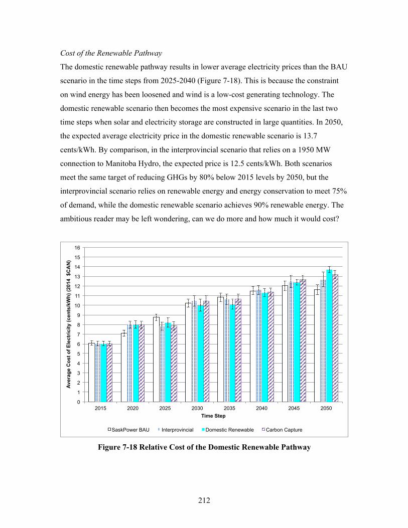
212

Cost of the Renewable Pathway

The domestic renewable pathway results in lower average electricity prices than the BAU

scenario in the time steps from 2025-2040 (Figure 7-18). This is because the constraint

on wind energy has been loosened and wind is a low-cost generating technology. The

domestic renewable scenario then becomes the most expensive scenario in the last two

time steps when solar and electricity storage are constructed in large quantities. In 2050,

the expected average electricity price in the domestic renewable scenario is 13.7

cents/kWh. By comparison, in the interprovincial scenario that relies on a 1950 MW

connection to Manitoba Hydro, the expected price is 12.5 cents/kWh. Both scenarios

meet the same target of reducing GHGs by 80% below 2015 levels by 2050, but the

interprovincial scenario relies on renewable energy and energy conservation to meet 75%

of demand, while the domestic renewable scenario achieves 90% renewable energy. The

ambitious reader may be left wondering, can we do more and how much it would cost?

Figure 7-18 Relative Cost of the Domestic Renewable Pathway

0

1

2

3

4

5

6

7

8

9

10

11

12

13

14

15

16

2015 2020 2025 2030 2035 2040 2045 2050

Ave

rage

Cos

t of E

lect

rici

ty (c

ents

/kW

h) (2

014

$C

AN

)

Time Step

SaskPower BAU Interprovincial Domestic Renewable Carbon Capture

213

Greening the Saskatchewan Grid

As a last task in this Chapter I ask, how much would it cost to achieve an aggressive

GHG reduction strategy? This strategy would not wait until 2045 to pursue renewable

energy and would instead see SaskPower undertake a complete transformation of the grid

in the period following the retirement of Saskatchewan’s coal-fired power plants in 2030.

This scenario would achieve near-zero GHG emissions by 2040. It would see

conventional coal phased out by 2030, and conventional natural gas facilities phased out

by 2040. Renewable energy and energy conservation would meet 78% of electricity

demand by 2030, 94% by 2040 and 95% by 2050. This achievement would make

Saskatchewan one of the leaders in renewable electricity generation in Canada and the

world.

In this Greening the Saskatchewan Grid scenario, I allow imports of 1950 MW of power

from Manitoba Hydro. As the scenarios above show, this helps to keep electricity rates

low and helps to balance variable wind and solar energy. I retire the Shand coal-fired

power plant in 2025, rather than retrofitting it to run until 2045. I allow wind-powered

electricity to meet 24% of total demand by 2030 and 35% by 2050. I then constrain the

model to reduce GHGs to 100 kt CO2e by 2040. When the resulting Greening the Grid

scenario was tested in WIRE it ran in each of the four representative months. This Green

Grid scenario is presented in Figure 7-19.

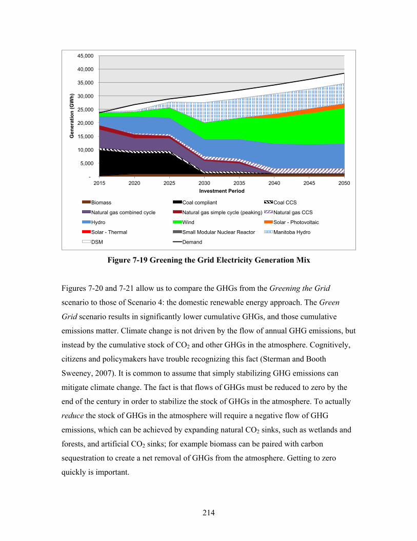
214

Figure 7-19 Greening the Grid Electricity Generation Mix

Figures 7-20 and 7-21 allow us to compare the GHGs from the Greening the Grid

scenario to those of Scenario 4: the domestic renewable energy approach. The Green

Grid scenario results in significantly lower cumulative GHGs, and those cumulative

emissions matter. Climate change is not driven by the flow of annual GHG emissions, but

instead by the cumulative stock of CO2 and other GHGs in the atmosphere. Cognitively,

citizens and policymakers have trouble recognizing this fact (Sterman and Booth

Sweeney, 2007). It is common to assume that simply stabilizing GHG emissions can

mitigate climate change. The fact is that flows of GHGs must be reduced to zero by the

end of the century in order to stabilize the stock of GHGs in the atmosphere. To actually

reduce the stock of GHGs in the atmosphere will require a negative flow of GHG

emissions, which can be achieved by expanding natural CO2 sinks, such as wetlands and

forests, and artificial CO2 sinks; for example biomass can be paired with carbon

sequestration to create a net removal of GHGs from the atmosphere. Getting to zero

quickly is important.

-

5,000

10,000

15,000

20,000

25,000

30,000

35,000

40,000

45,000

2015 2020 2025 2030 2035 2040 2045 2050

Gen

erat

ion

(GW

h)

Investment Period

Biomass Coal compliant Coal CCS

Natural gas combined cycle Natural gas simple cycle (peaking) Natural gas CCS

Hydro Wind Solar - Photovoltaic

Solar - Thermal Small Modular Nuclear Reactor Manitoba Hydro

DSM Demand

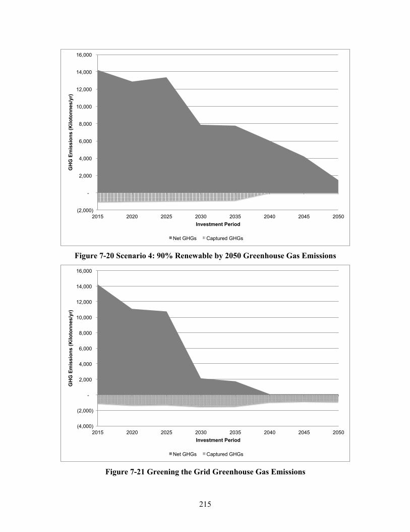
215

Figure 7-20 Scenario 4: 90% Renewable by 2050 Greenhouse Gas Emissions

Figure 7-21 Greening the Grid Greenhouse Gas Emissions

(2,000)

-

2,000

4,000

6,000

8,000

10,000

12,000

14,000

16,000

2015 2020 2025 2030 2035 2040 2045 2050

GH

G E

mis

sion

s (K

iloto

nnes

/yr)

Investment Period

Net GHGs Captured GHGs

(4,000)

(2,000)

-

2,000

4,000

6,000

8,000

10,000

12,000

14,000

16,000

2015 2020 2025 2030 2035 2040 2045 2050

GH

G E

mis

sion

s (K

iloto

nnes

/yr)

Investment Period

Net GHGs Captured GHGs

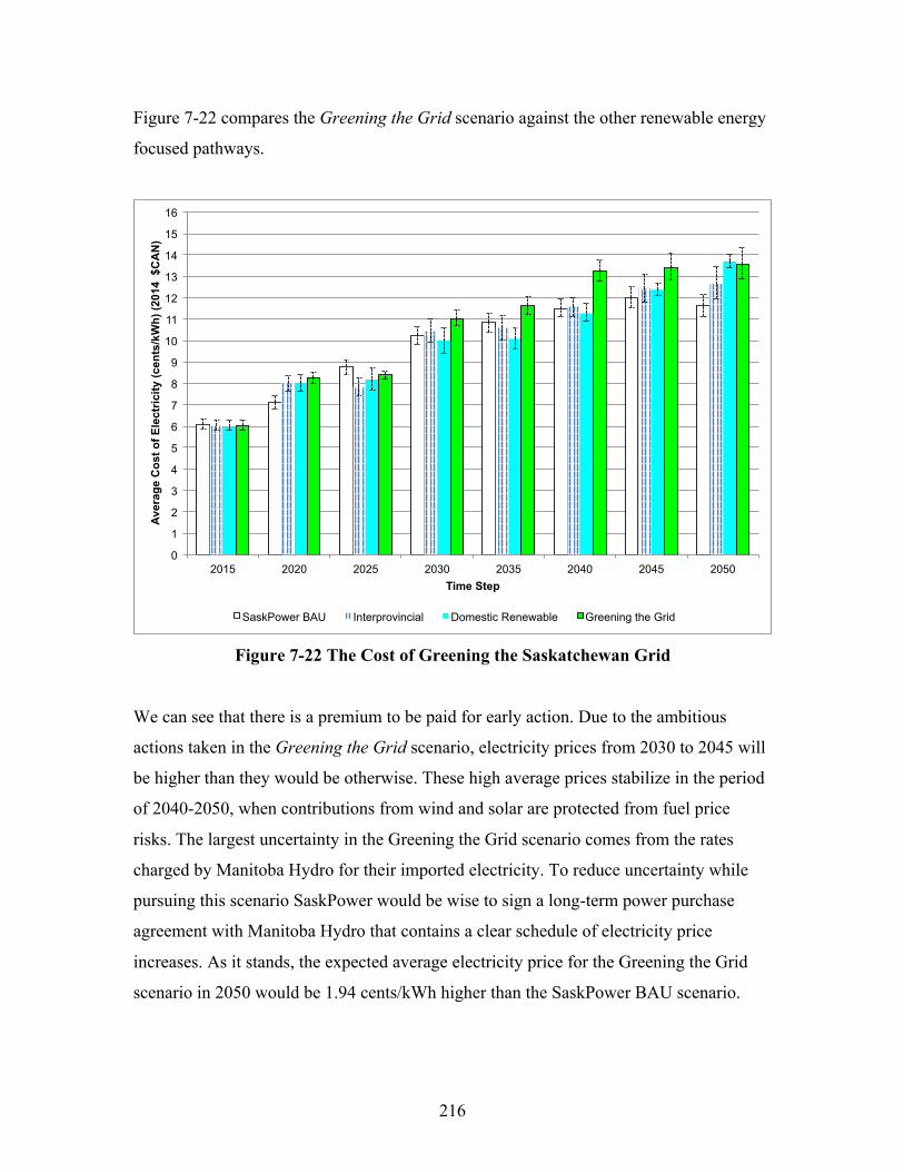
216

Figure 7-22 compares the Greening the Grid scenario against the other renewable energy

focused pathways.

Figure 7-22 The Cost of Greening the Saskatchewan Grid

We can see that there is a premium to be paid for early action. Due to the ambitious

actions taken in the Greening the Grid scenario, electricity prices from 2030 to 2045 will

be higher than they would be otherwise. These high average prices stabilize in the period

of 2040-2050, when contributions from wind and solar are protected from fuel price

risks. The largest uncertainty in the Greening the Grid scenario comes from the rates

charged by Manitoba Hydro for their imported electricity. To reduce uncertainty while

pursuing this scenario SaskPower would be wise to sign a long-term power purchase

agreement with Manitoba Hydro that contains a clear schedule of electricity price

increases. As it stands, the expected average electricity price for the Greening the Grid

scenario in 2050 would be 1.94 cents/kWh higher than the SaskPower BAU scenario.

0

1

2

3

4

5

6

7

8

9

10

11

12

13

14

15

16

2015 2020 2025 2030 2035 2040 2045 2050

Ave

rage

Cos

t of E

lect

rici

ty (c

ents

/kW

h) (2

014

$C

AN

)

Time Step

SaskPower BAU Interprovincial Domestic Renewable Greening the Grid

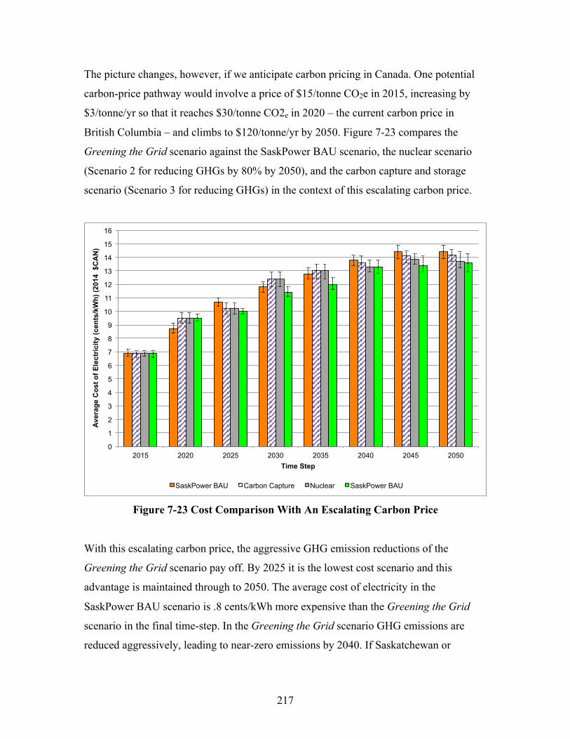
217

The picture changes, however, if we anticipate carbon pricing in Canada. One potential

carbon-price pathway would involve a price of $15/tonne CO2e in 2015, increasing by

$3/tonne/yr so that it reaches $30/tonne CO2e in 2020 – the current carbon price in

British Columbia – and climbs to $120/tonne/yr by 2050. Figure 7-23 compares the

Greening the Grid scenario against the SaskPower BAU scenario, the nuclear scenario

(Scenario 2 for reducing GHGs by 80% by 2050), and the carbon capture and storage

scenario (Scenario 3 for reducing GHGs) in the context of this escalating carbon price.

Figure 7-23 Cost Comparison With An Escalating Carbon Price

With this escalating carbon price, the aggressive GHG emission reductions of the

Greening the Grid scenario pay off. By 2025 it is the lowest cost scenario and this

advantage is maintained through to 2050. The average cost of electricity in the

SaskPower BAU scenario is .8 cents/kWh more expensive than the Greening the Grid

scenario in the final time-step. In the Greening the Grid scenario GHG emissions are

reduced aggressively, leading to near-zero emissions by 2040. If Saskatchewan or

0

1

2

3

4

5

6

7

8

9

10

11

12

13

14

15

16

2015 2020 2025 2030 2035 2040 2045 2050

Ave

rage

Cos

t of E

lect

rici

ty (c

ents

/kW

h) (2

014

$C

AN

)

Time Step

SaskPower BAU Carbon Capture Nuclear SaskPower BAU

218

Canada were to implement carbon pricing the Greening the Grid scenario would be

resilient against a carbon pricing shock.

Conclusions

In this chapter I have compared SaskPower’s business-as-usual (BAU) electricity

generation plan against a range of other scenarios. The BAU scenario relies on

retrofitting coal-fired plants with carbon capture and storage (CCS) to meet federal coal-

fired regulations. I found that SaskPower could achieve the same level of GHG emissions

reductions at a lower cost by shutting down existing coal plants, investing in wind,

hydroelectric and natural gas facilities, and importing more hydroelectricity from

Manitoba Hydro. Over the period of 2030-2050 this equivalency approach saves .86

cents/kWh relative to SaskPower approach. However, both the BAU and equivalency

scenarios do not lead to lasting GHG emissions reductions. By 2045 GHG emissions

begin to increase in both scenarios.

I then explored four scenarios for achieving an 80% reduction in GHG emissions by

2050: an interprovincial approach, which took advantage of low-cost Manitoba Hydro

imports; a nuclear approach, in which 1000 MW of small, modular reactor capacity was

built by 2050; a carbon capture approach, which relies on investment in natural gas with

CCS; and a domestic renewable energy scenario, which meets Saskatchewan’s electricity

demand with investments in wind, solar, domestic hydroelectric facilities, electricity

storage, and energy conservation. Each of these scenarios achieved the goal of reducing

GHG emissions by 80% relative to 2015 by 2050. Each scenario also proved capable of

reliably supplying electricity when tested using the WIRE model. Electricity generation

costs were higher than the SaskPower BAU scenario by 2050, but not significantly so;

there was, for example, still overlap between the 95% confidence interval of the

interprovincial scenario and the SaskPower BAU scenario.

Lastly, I outlined a Greening the Grid scenario in which Saskatchewan moves quickly to

phase out coal-fired electricity generation by 2030 and achieves near-zero GHG

emissions by 2040 using predominantly renewable energy technologies. This scenario

219

required careful and iterative planning; higher penetrations of renewables meant that I

had to pay attention to a ‘Liebig’s Law of the Minimum’ rule related to seasonal solar

and hydroelectric potential. After iterating between SIM and WIRE, I found a scenario

that could reliably meet Saskatchewan’s hourly electricity demand in four representative

months of March, June, September and December. In this WIRE simulation a

combination of electricity storage, demand side management, and fast-ramping

hydroelectric generation capacity (located both within Saskatchewan and imported from

Manitoba) allowed high penetrations of variable wind and solar to be integrated onto the

Saskatchewan grid.

The Greening the Grid scenario did increase the average cost of electricity generation by

1.94 cents/kwh relative to the SaskPower BAU scenario. However, with an escalating

carbon price, the Greening the Grid scenario becomes the lowest cost electricity pathway.

In any scenario, electricity generation costs are anticipated to rise in the future. In the

next chapter I explore the implications of this price increase on individuals, businesses,

and industry in the province. I also outline scenario impacts that are more difficult, or in

some cases impossible, to express in financial terms. These impacts are relevant to a

public discussion of Saskatchewan’s electricity future.

220

Chapter 8 – Scenario Impacts

Introduction

The scenarios outlined in Chapter 7 differ in terms of their projected cost of electricity

and their greenhouse gas (GHG) emissions. In this chapter I compare the scenarios using

a selection of other criteria. My aim is to begin to assess the sustainability of each

scenario. A sustainability assessment is, however, an evaluation process that is best

undertaken with widespread public input and deliberation (Winfield et al., 2010). White

and Noble (2012) provide a good example of a quantitative approach to strategic

environmental assessment that could form the basis of a larger public consultation. In this

chapter I limit my efforts to providing quantitative indicators and qualitative commentary

that can guide a future public sustainability assessment.

Sustainability Criteria

There are a number of criteria with which the sustainability of electricity scenarios can be

evaluated. Jaccard (2005) uses four criteria to evaluate energy technology options:

projected cost, extreme event risk, geopolitical risk, and path dependence. The first two

criteria are fairly self-explanatory; I outlined projected cost for each scenario in Chapter 7

and extreme event risk relates to the possibility that an extreme event may affect the

stability of the system or the health and safety of the public. Geopolitical risk is relevant

in international markets such as oil, where supply chains can be disrupted by cartels and

political embargoes. It is less relevant in an assessment of Saskatchewan electricity;

supplies of coal, uranium, and natural gas are produced locally and are not vulnerable to

international supply risks. One might, however, reframe this criterion as energy

independence. Premier Brad Wall has expressed his interest in continued use of coal in

order to maintain energy independence (Zinchuk, 2014). Imports of hydroelectricity from

Manitoba are interpreted as reducing energy independence. For Jaccard (2005) the fourth

criterion, path dependence, is a measure of the degree of fit between a proposed

electricity system and an existing system. Scenarios that fit within an existing socio-

political-technical institutional context will face lower resistance to adoption than

scenarios that disrupt existing institutional arrangements.

221

Winfield et al. (2010) critique Jaccard’s (2005) criteria (and other related criteria) for

focusing on economic and technical characteristics and “neglecting equity effects,

systemic interactions and uncertainty/precautionary factors” (p. 4119). Winfield et al.

(2010) propose a detailed set of eight criteria that can be applied in a sustainability

assessment, as well as six trade-off rules or principles that should be followed when

choosing between scenarios. The eight criteria that should be considered in a

sustainability assessment are listed below. I include a short quote or summary relevant to

each criterion to indicate its meaning:

1. Socio-ecological system integrity – “protect irreplaceable life support functions”

2. Livelihood sufficiency and opportunity – “Ensure that everyone and every

community has enough for a decent life”

3. Intragenerational equity – “reduce dangerous gaps in sufficiency and

opportunity…between the rich and poor”

4. Intergenerational equity – “enhance the opportunities and capabilities of future

generations to live sustainably”

5. Resource maintenance and efficiency – reduce extractive damage, avoid waste,

and improve efficiency

6. Socio-ecological civility and democratic governance – “apply sustainability

requirements through more open and better-informed deliberations”

7. Precaution and adaptation – “Respect uncertainty, and avoid even poorly

understood risks of serious or irreversible damage”

8. Immediate and long-term integration – “Apply all principles of sustainability at

once”

(Winfield et al., 2010: 4119)

When two scenarios both pose a threat to any of these criteria it is necessary to consider

trade-offs. The six rules for trade-offs outlined by Winfield et al. (2010) include:

• Burden of argument on trade-off proponent – “the burden of justification falls on

the proponent of the trade-off”

222

• Avoidance of significant adverse effects – “No trade-off that involves a

significant adverse effect…can be justified unless the alternative is acceptance of

an even more significant adverse effect.”

(Winfield et al., 2010: 2119)

The remaining trade-off rules call for decision-makers to seek maximum net gains,

protect the future, explicitly and openly justify trade-off decisions, and evaluate trade-

offs in “processes that include open and effective involvement of all stakeholders” (p.

4119).

White and Noble (2012) used eight criteria in their strategic environmental assessment of

Saskatchewan’s electricity system. These criteria bear resemblance to Winfield et al.

(2010) in that they strive to address equity, but also included is the criterion “security of

supply” which is akin to Jaccard’s (2005) “geopolitical risk” criterion. The eight criteria

used by White and Noble (2012) are as follows:

1. Adaptive capacity – “Maximizes the ability to accommodate projected, as well as

unanticipated future demand growth”

2. Emissions management – “Minimizes emissions to air and water during electricity

production, distribution and use over the life cycle of the system”

3. Employment and income sufficiency – “Maximizes short- and long-term income

and employment opportunities”

4. Ecological integrity – “Ensures biodiversity conservation and ecological

resiliency by minimizing use and disturbance of land and water resources”

5. Security of supply – “Ensures secure and affordable access to energy supply for

current and future generations”

6. Energy production and transmission efficiency – “Meets electricity demands

while minimizing energy use, raw material use and generation of waste during

production and energy loss during transmission”

7. Aboriginal rights – “Minimizes infringement on culture, traditional land use

practices and Treaty Rights”

223

8. Public health and safety – “Minimizes risk to public health and safety during

electricity production and transmission.”

(White and Noble, 2012: 286)

While Winfield et al. (2010 and White and Noble (2012) share some overlapping criteria

like “ecological integrity”, there are important differences. White and Noble’s (2012)

definition of adaptive capacity appears biased towards electricity system growth. They

are concerned with efficiency, but define efficiency with respect to “energy production

and transmission efficiency”, not in terms of energy demand. Winfield et al. (2010)

emphasize energy conservation in their definition of resource maintenance and efficiency

when they speak of “reducing overall material and energy use per unit benefit” (p. 4119).

As well, Winfield et al (2010) recommend an integrative approach to assessment. The

language used in White and Noble’s (2012) list is the language of optimization; each

criterion is either maximized or minimized. In their strategic environmental assessment,

White and Noble (2010) had expert participants weigh and rank the criteria. These

weighted criteria were then used to create a score for each scenario. This reductionist

approach reduces opportunities for an integrative view of scenario selection.

White and Noble (2012) do however, consider important factors that are implied by

criteria listed by Winfield et al. (2010), but not explicitly stated. In particular, the

criterion ‘Aboriginal rights’ is very relevant in Saskatchewan, which has a high

proportion of people identifying as aboriginal in its population (15.6% in 2011, Statistics

Canada, 2011b). The Canadian constitution recognizes aboriginal rights and treaty rights,

which include the right to traditional livelihoods. The Canadian courts have ruled that

government has a duty to consult and accommodate aboriginal peoples on decisions that

may impact their livelihoods (Aboriginal Affairs, 2011). Electricity sector projects can

impact aboriginal livelihoods (e.g. the E.B. Campbell hydroelectric station affected

fishing for aboriginals downstream of the dam). Recognition of aboriginal rights and

interests has led SaskPower to seek partnerships with First Nations on power projects like

the proposed Tazi Twé hydroelectric station.

224

In this chapter I offer quantitative indicators that can contribute to understanding the

sustainability criteria outlined above. The quantitative indicators I provide for each

scenario are listed below and grouped by the criterion they help to inform.68

• Projected Costs (Jaccard, 2005)

o Projected cost of electricity in 2050 with and without carbon pricing

(cents/kwh);

o Total discounted cost of meeting electricity demand 2015-2050 with and

without carbon pricing ($Millions).

• Intragenerational equity (Winfield et al, 2010):

o Electricity rate impacts to residential customers (cents/kwh); and

o Electricity rate impacts to commercial customers (cents/kwh).

• Livelihood sufficiency and opportunity (Winfield et al, 2010):

o Electricity rate impacts to industrial customers (cents/kwh);

o Direct and indirect employment resulting from the electricity scenarios

(full-time jobs);

o Direct and indirect employment divided by electricity price to control for

scenario cost (full-time jobs/cents per kwh).

• Emissions management (White and Noble, 2012):

o Annual direct GHG emissions in 2050 (kilotonnes CO2e);

o Cumulative direct GHG emissions 2015-2050 (Megatonnes CO2e);

o Cumulative captured CO2 (km3).

• Ecological integrity (Winfield et al., 2010; White and Noble, 2012):

o Land impacted by wind and solar facilities (Sections/hectares);

o Water consumption by all facilities (Gigalitre/Olympic sized pool);

o Hydroelectricity capacity in Saskatchewan (MW);

o Hydroelectric dams on the Churchill River (number).

• Energy Independence (modified from Jaccard, 2005)

o Hydroelectric contracts with Manitoba Hydro (MW).

• Resource maintenance and efficiency (Winfield et al., 2010) 68 All monetary values are reported in 2014 $CAN constant dollars.

225

o DSM energy savings in 2050 (GWh)

• Precaution (Winfield et al., 2010) and public health and safety (White and Noble,

2012):

o Radioactive waste produced by nuclear power production (tonnes).

These indicators are far from comprehensive, but touch on some of the key issues

associated with the various electricity scenarios. For instance, while I give only a passing

reference to the land impacts related to coal-fired generation, and do not comment on the

land impacts related to natural gas-fired generation (including natural gas extraction),

nuclear power (including uranium mining), hydroelectricity generation, or biomass, I list

land impacted by wind and solar facilities because these energy sources are often singled

out for their low “energy density” (e.g. van Kooten, 2011). The measure of land impacted

by wind and solar provides a quantitative indicator that can inform a discussion of energy

density and land-use impact. As well, when I explore employment impacts, I use data for

both direct and indirect employment. However, when I outline cumulative GHG

emissions I focus only on direct emissions at the site of electricity production, and not

indirect emissions associated with manufacturing and installing a technology, or

decommissioning a facility and dealing with its waste. Water use is a measure of direct

use during operation and does not include the water associated with manufacturing the

technologies. After presenting a selection of these indicators I discuss how they might

contribute to our understanding of the sustainability of each electricity scenario.

Projected Costs

In Chapter 7 I presented the electricity cost resulting from each scenario. A summary of

the electricity costs in 2050 is presented in Table 8-1. These indicators contribute to

understanding Jaccard’s (2005) sustainability criterion of projected cost. The lowest cost

scenarios are highlighted in light blue while the highest cost scenarios for each indicator

are highlighted in rose.

The section marked ‘Projected Cost’ outlines the expected cost of electricity in 2050,

along with the 95% and 5% confidence intervals from the sensitivity analysis. The BAU

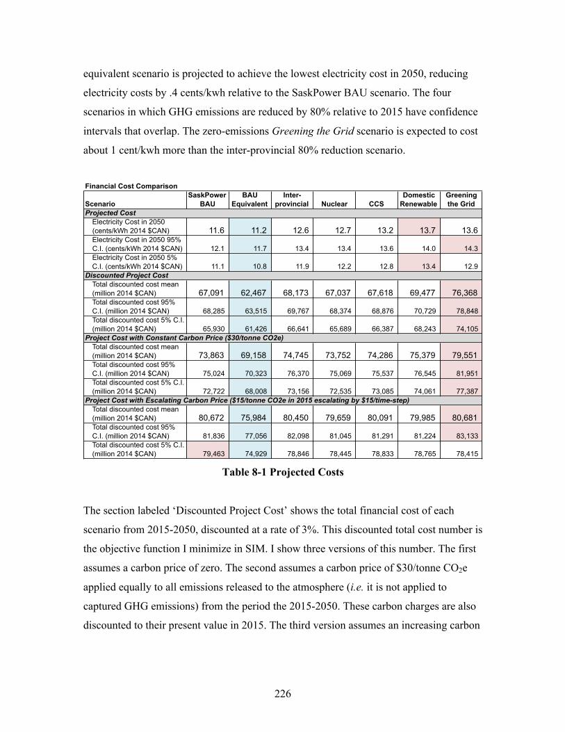
226

equivalent scenario is projected to achieve the lowest electricity cost in 2050, reducing

electricity costs by .4 cents/kwh relative to the SaskPower BAU scenario. The four

scenarios in which GHG emissions are reduced by 80% relative to 2015 have confidence

intervals that overlap. The zero-emissions Greening the Grid scenario is expected to cost

about 1 cent/kwh more than the inter-provincial 80% reduction scenario.

Table 8-1 Projected Costs

The section labeled ‘Discounted Project Cost’ shows the total financial cost of each

scenario from 2015-2050, discounted at a rate of 3%. This discounted total cost number is

the objective function I minimize in SIM. I show three versions of this number. The first

assumes a carbon price of zero. The second assumes a carbon price of $30/tonne CO2e

applied equally to all emissions released to the atmosphere (i.e. it is not applied to

captured GHG emissions) from the period the 2015-2050. These carbon charges are also

discounted to their present value in 2015. The third version assumes an increasing carbon

Financial Cost Comparison

ScenarioSaskPower

BAU BAU

EquivalentInter-

provincial Nuclear CCSDomestic

RenewableGreening the Grid

Electricity Cost in 2050 (cents/kWh 2014 $CAN) 11.6 11.2 12.6 12.7 13.2 13.7 13.6 Electricity Cost in 2050 95% C.I. (cents/kWh 2014 $CAN) 12.1 11.7 13.4 13.4 13.6 14.0 14.3 Electricity Cost in 2050 5% C.I. (cents/kWh 2014 $CAN) 11.1 10.8 11.9 12.2 12.8 13.4 12.9

Total discounted cost mean (million 2014 $CAN) 67,091 62,467 68,173 67,037 67,618 69,477 76,368 Total discounted cost 95% C.I. (million 2014 $CAN) 68,285 63,515 69,767 68,374 68,876 70,729 78,848 Total discounted cost 5% C.I. (million 2014 $CAN) 65,930 61,426 66,641 65,689 66,387 68,243 74,105

Total discounted cost mean (million 2014 $CAN) 73,863 69,158 74,745 73,752 74,286 75,379 79,551 Total discounted cost 95% C.I. (million 2014 $CAN) 75,024 70,323 76,370 75,069 75,537 76,545 81,951 Total discounted cost 5% C.I. (million 2014 $CAN) 72,722 68,008 73,156 72,535 73,085 74,061 77,387

Total discounted cost mean (million 2014 $CAN) 80,672 75,984 80,450 79,659 80,091 79,985 80,681 Total discounted cost 95% C.I. (million 2014 $CAN) 81,836 77,056 82,098 81,045 81,291 81,224 83,133 Total discounted cost 5% C.I. (million 2014 $CAN) 79,463 74,929 78,846 78,445 78,833 78,765 78,415

Projected Cost

Discounted Project Cost

Project Cost with Constant Carbon Price ($30/tonne CO2e)

Project Cost with Escalating Carbon Price ($15/tonne CO2e in 2015 escalating by $15/time-step)

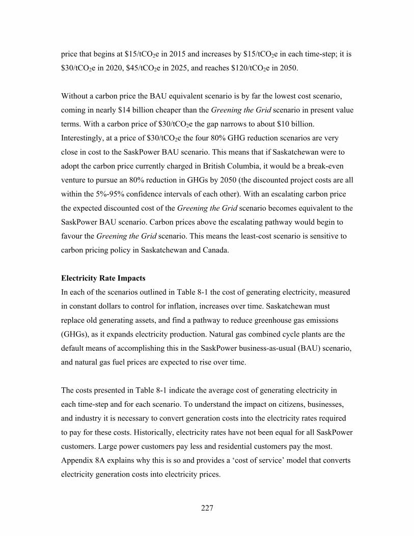
227

price that begins at $15/tCO2e in 2015 and increases by $15/tCO2e in each time-step; it is

$30/tCO2e in 2020, $45/tCO2e in 2025, and reaches $120/tCO2e in 2050.

Without a carbon price the BAU equivalent scenario is by far the lowest cost scenario,

coming in nearly $14 billion cheaper than the Greening the Grid scenario in present value

terms. With a carbon price of $30/tCO2e the gap narrows to about $10 billion.

Interestingly, at a price of $30/tCO2e the four 80% GHG reduction scenarios are very

close in cost to the SaskPower BAU scenario. This means that if Saskatchewan were to

adopt the carbon price currently charged in British Columbia, it would be a break-even

venture to pursue an 80% reduction in GHGs by 2050 (the discounted project costs are all

within the 5%-95% confidence intervals of each other). With an escalating carbon price

the expected discounted cost of the Greening the Grid scenario becomes equivalent to the

SaskPower BAU scenario. Carbon prices above the escalating pathway would begin to

favour the Greening the Grid scenario. This means the least-cost scenario is sensitive to

carbon pricing policy in Saskatchewan and Canada.

Electricity Rate Impacts

In each of the scenarios outlined in Table 8-1 the cost of generating electricity, measured

in constant dollars to control for inflation, increases over time. Saskatchewan must

replace old generating assets, and find a pathway to reduce greenhouse gas emissions

(GHGs), as it expands electricity production. Natural gas combined cycle plants are the

default means of accomplishing this in the SaskPower business-as-usual (BAU) scenario,

and natural gas fuel prices are expected to rise over time.

The costs presented in Table 8-1 indicate the average cost of generating electricity in

each time-step and for each scenario. To understand the impact on citizens, businesses,

and industry it is necessary to convert generation costs into the electricity rates required

to pay for these costs. Historically, electricity rates have not been equal for all SaskPower

customers. Large power customers pay less and residential customers pay the most.

Appendix 8A explains why this is so and provides a ‘cost of service’ model that converts

electricity generation costs into electricity prices.

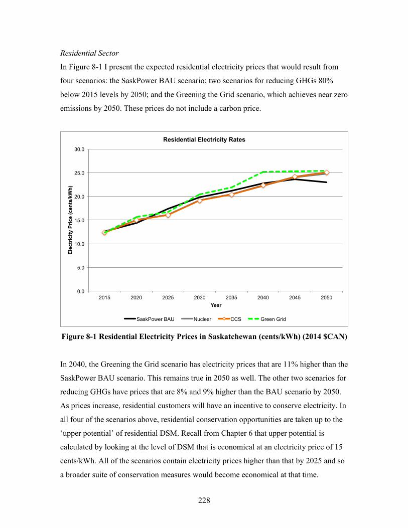
228

Residential Sector

In Figure 8-1 I present the expected residential electricity prices that would result from

four scenarios: the SaskPower BAU scenario; two scenarios for reducing GHGs 80%

below 2015 levels by 2050; and the Greening the Grid scenario, which achieves near zero

emissions by 2050. These prices do not include a carbon price.

Figure 8-1 Residential Electricity Prices in Saskatchewan (cents/kWh) (2014 $CAN)

In 2040, the Greening the Grid scenario has electricity prices that are 11% higher than the

SaskPower BAU scenario. This remains true in 2050 as well. The other two scenarios for

reducing GHGs have prices that are 8% and 9% higher than the BAU scenario by 2050.

As prices increase, residential customers will have an incentive to conserve electricity. In

all four of the scenarios above, residential conservation opportunities are taken up to the

‘upper potential’ of residential DSM. Recall from Chapter 6 that upper potential is

calculated by looking at the level of DSM that is economical at an electricity price of 15

cents/kWh. All of the scenarios contain electricity prices higher than that by 2025 and so

a broader suite of conservation measures would become economical at that time.

0.0

5.0

10.0

15.0

20.0

25.0

30.0

2015 2020 2025 2030 2035 2040 2045 2050

Elec

tric

ity P

rice

(cen

ts/k

Wh)

Year

Residential Electricity Rates

SaskPower BAU Nuclear CCS Green Grid

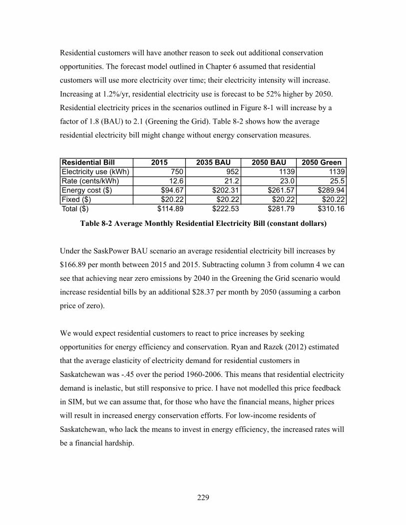
229

Residential customers will have another reason to seek out additional conservation

opportunities. The forecast model outlined in Chapter 6 assumed that residential

customers will use more electricity over time; their electricity intensity will increase.

Increasing at 1.2%/yr, residential electricity use is forecast to be 52% higher by 2050.

Residential electricity prices in the scenarios outlined in Figure 8-1 will increase by a

factor of 1.8 (BAU) to 2.1 (Greening the Grid). Table 8-2 shows how the average

residential electricity bill might change without energy conservation measures.

Table 8-2 Average Monthly Residential Electricity Bill (constant dollars)

Under the SaskPower BAU scenario an average residential electricity bill increases by

$166.89 per month between 2015 and 2015. Subtracting column 3 from column 4 we can

see that achieving near zero emissions by 2040 in the Greening the Grid scenario would

increase residential bills by an additional $28.37 per month by 2050 (assuming a carbon

price of zero).

We would expect residential customers to react to price increases by seeking

opportunities for energy efficiency and conservation. Ryan and Razek (2012) estimated

that the average elasticity of electricity demand for residential customers in

Saskatchewan was -.45 over the period 1960-2006. This means that residential electricity

demand is inelastic, but still responsive to price. I have not modelled this price feedback

in SIM, but we can assume that, for those who have the financial means, higher prices

will result in increased energy conservation efforts. For low-income residents of

Saskatchewan, who lack the means to invest in energy efficiency, the increased rates will

be a financial hardship.

Residential Bill 2015 2035 BAU 2050 BAU 2050 GreenElectricity use (kWh) 750 952 1139 1139Rate (cents/kWh) 12.6 21.2 23.0 25.5Energy cost ($) $94.67 $202.31 $261.57 $289.94Fixed ($) $20.22 $20.22 $20.22 $20.22Total ($) $114.89 $222.53 $281.79 $310.16

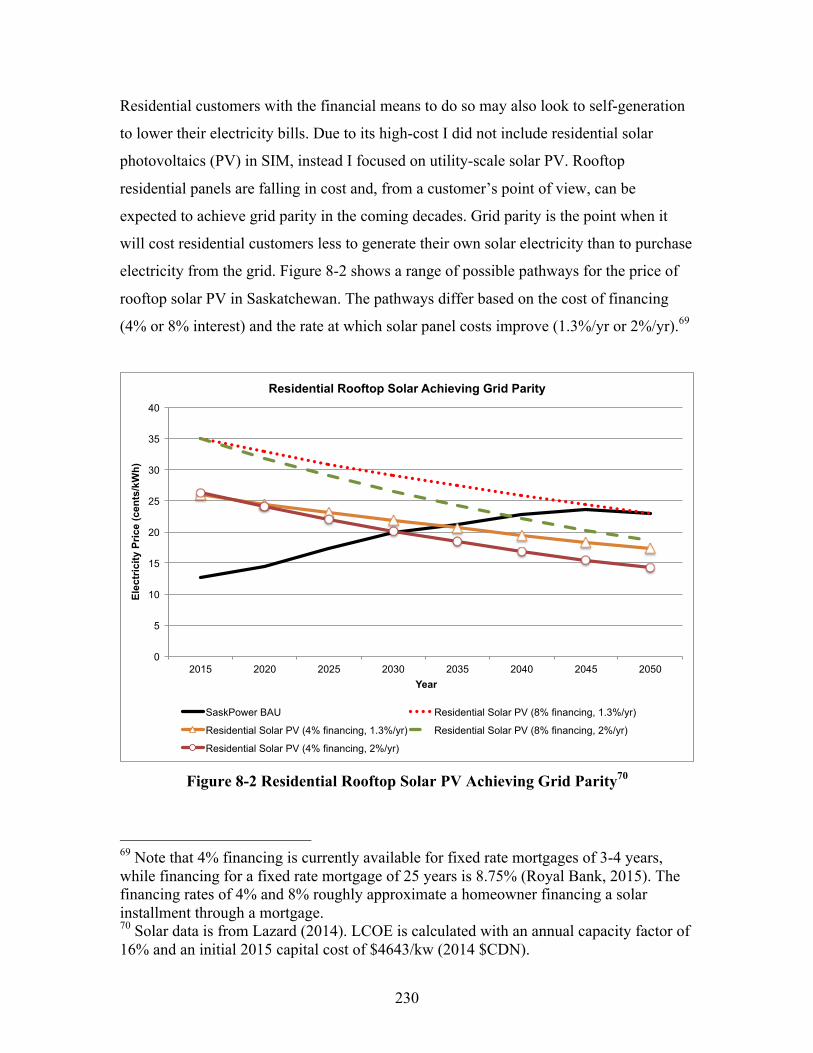
230

Residential customers with the financial means to do so may also look to self-generation

to lower their electricity bills. Due to its high-cost I did not include residential solar

photovoltaics (PV) in SIM, instead I focused on utility-scale solar PV. Rooftop

residential panels are falling in cost and, from a customer’s point of view, can be

expected to achieve grid parity in the coming decades. Grid parity is the point when it

will cost residential customers less to generate their own solar electricity than to purchase

electricity from the grid. Figure 8-2 shows a range of possible pathways for the price of

rooftop solar PV in Saskatchewan. The pathways differ based on the cost of financing

(4% or 8% interest) and the rate at which solar panel costs improve (1.3%/yr or 2%/yr).69

Figure 8-2 Residential Rooftop Solar PV Achieving Grid Parity70

69 Note that 4% financing is currently available for fixed rate mortgages of 3-4 years, while financing for a fixed rate mortgage of 25 years is 8.75% (Royal Bank, 2015). The financing rates of 4% and 8% roughly approximate a homeowner financing a solar installment through a mortgage. 70 Solar data is from Lazard (2014). LCOE is calculated with an annual capacity factor of 16% and an initial 2015 capital cost of $4643/kw (2014 $CDN).

0

5

10

15

20

25

30

35

40

2015 2020 2025 2030 2035 2040 2045 2050

Ele

ctri

city

Pri

ce (c

ents

/kW

h)

Year

Residential Rooftop Solar Achieving Grid Parity

SaskPower BAU Residential Solar PV (8% financing, 1.3%/yr)

Residential Solar PV (4% financing, 1.3%/yr) Residential Solar PV (8% financing, 2%/yr)

Residential Solar PV (4% financing, 2%/yr)

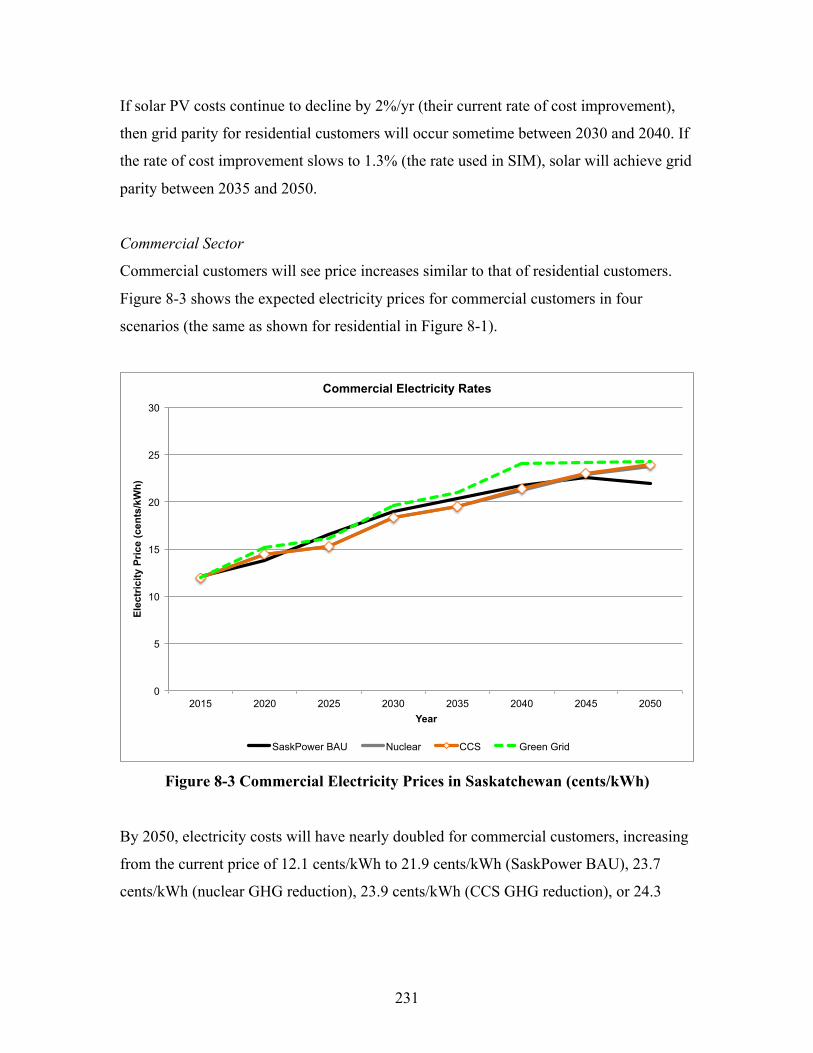
231

If solar PV costs continue to decline by 2%/yr (their current rate of cost improvement),

then grid parity for residential customers will occur sometime between 2030 and 2040. If

the rate of cost improvement slows to 1.3% (the rate used in SIM), solar will achieve grid

parity between 2035 and 2050.

Commercial Sector

Commercial customers will see price increases similar to that of residential customers.

Figure 8-3 shows the expected electricity prices for commercial customers in four

scenarios (the same as shown for residential in Figure 8-1).

Figure 8-3 Commercial Electricity Prices in Saskatchewan (cents/kWh)

By 2050, electricity costs will have nearly doubled for commercial customers, increasing

from the current price of 12.1 cents/kWh to 21.9 cents/kWh (SaskPower BAU), 23.7

cents/kWh (nuclear GHG reduction), 23.9 cents/kWh (CCS GHG reduction), or 24.3

0

5

10

15

20

25

30

2015 2020 2025 2030 2035 2040 2045 2050

Ele

ctri

city

Pri

ce (c

ents

/kW

h)

Year

Commercial Electricity Rates

SaskPower BAU Nuclear CCS Green Grid

232

cents/kWh (Green Grid).71 Table 8-3 shows the impact these higher prices would have on

the average monthly commercial electricity bill.

Table 8-3 Average Monthly Commercial Electricity Bill

In the commercial sector the impact of increasing prices is muted by improvements in

energy efficiency. In Chapter 6 I forecast that electricity use in the commercial sector

would decline at a rate of 1.2%/yr. This leads electricity use to about 2/3 the 2015 level

by 2050. Additional energy conservation measures could be undertaken above and

beyond that assumed rate of change to further control cost increases.

71 These estimates of price increases do not account for uncertainty and do not include a carbon price. Refer to Chapter 7 for the range of potential price increases that would result from each scenario and to see the impact of carbon pricing.

Commercial Bill 2015 2035 BAU 2050 BAU 2050 GreenElectricity use (kWh) 6000 4713 3932 3932Rate (cents/kWh) 12.1 20.3 21.9 24.3Energy cost ($) $727.54 $955.87 $862.18 $955.54Fixed ($) $20.22 $20.22 $20.22 $20.22Total ($) $747.76 $976.09 $882.40 $975.76

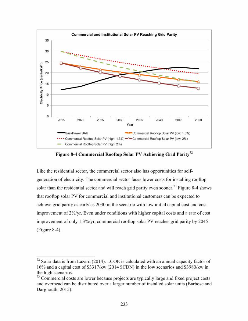
233

Figure 8-4 Commercial Rooftop Solar PV Achieving Grid Parity72

Like the residential sector, the commercial sector also has opportunities for self-

generation of electricity. The commercial sector faces lower costs for installing rooftop

solar than the residential sector and will reach grid parity even sooner.73 Figure 8-4 shows

that rooftop solar PV for commercial and institutional customers can be expected to

achieve grid parity as early as 2030 in the scenario with low initial capital cost and cost

improvement of 2%/yr. Even under conditions with higher capital costs and a rate of cost

improvement of only 1.3%/yr, commercial rooftop solar PV reaches grid parity by 2045

(Figure 8-4).

72 Solar data is from Lazard (2014). LCOE is calculated with an annual capacity factor of 16% and a capital cost of $3317/kw (2014 $CDN) in the low scenarios and $3980/kw in the high scenarios. 73 Commercial costs are lower because projects are typically large and fixed project costs and overhead can be distributed over a larger number of installed solar units (Barbose and Darghouth, 2015).

0

5

10

15

20

25

30

35

2015 2020 2025 2030 2035 2040 2045 2050

Ele

ctri

city

Pri

ce (c

ents

/kW

h)

Year

Commercial and Institutional Solar PV Reaching Grid Parity

SaskPower BAU Commercial Rooftop Solar PV (low, 1.3%)

Commercial Rooftop Solar PV (high, 1.3%) Commercial Rooftop Solar PV (low, 2%)

Commercial Rooftop Solar PV (high, 2%)

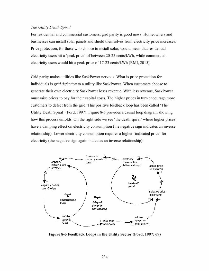
234

The Utility Death Spiral

For residential and commercial customers, grid parity is good news. Homeowners and

businesses can install solar panels and shield themselves from electricity price increases.

Price protection, for those who choose to install solar, would mean that residential

electricity users hit a ‘peak price’ of between 20-25 cents/kWh, while commercial

electricity users would hit a peak price of 17-23 cents/kWh (RMI, 2015).

Grid parity makes utilities like SaskPower nervous. What is price protection for

individuals is grid defection to a utility like SaskPower. When customers choose to

generate their own electricity SaskPower loses revenue. With less revenue, SaskPower

must raise prices to pay for their capital costs. The higher prices in turn encourage more

customers to defect from the grid. This positive feedback loop has been called ‘The

Utility Death Spiral’ (Ford, 1997). Figure 8-5 provides a causal loop diagram showing

how this process unfolds. On the right side we see ‘the death spiral’ where higher prices

have a damping effect on electricity consumption (the negative sign indicates an inverse

relationship). Lower electricity consumption requires a higher ‘indicated price’ for

electricity (the negative sign again indicates an inverse relationship).

Figure 8-5 Feedback Loops in the Utility Sector (Ford, 1997: 69)

Fig. 5. Key feedbackloops in the utilitysystem

reacted quickly and strongly to changes in the electric rate while they were stuckwith long lead time power plants under construction. Simply waiting for regulatorsto grant the requested rate increases would not necessarily solve their problems. Welearned that the utility could take steps on its own to soften the impact of the “deathspiral.” The best way to improve their situation was to shorten the length of theconstruction delay. This could be done by shifting investments from long lead timegeneration technologies (i.e., nuclear plants or large coal plants) to short lead timetechnologies (i.e., small coal plants, geothermal stations or wind machines). Wealso learned that the debilitating effects of the “death spiral” would be greatlyreduced if the IOU were expanding its system to keep pace with slow growth (i.e.,1–2 %/year) rather than the rapid growth of the “golden years.” Slower growth ratescould be achieved by utility conservation programs that would actively encouragetheir customers to invest in more efficient energy equipment.

1980s: the shift to small scale

The 1980s was a decade in which utilities shifted emphasis from large powerstations with long lead times to smaller, shorter lead time resources. Table 3 notesthat the move to smaller scale was manifest in:

• the cancellation of nuclear plants;• a shift to smaller coal plants;

Ford: System Dynamics and the Electric Power Industry 69

235

The death spiral is not an inevitable outcome for Saskatchewan. As one workshop

participant noted, grid defection leads to stranded assets; power plants that are

underutilized or that are shut down prematurely. But, as a crown corporation, these

stranded assets belong to the people of Saskatchewan (Workshop 1). SaskPower’s debt

sits on the Government of Saskatchewan’s books and Saskatchewan citizens and

businesses will have to pay for it either through electricity payments to SaskPower or

taxes at a later date. Anticipation of the death spiral may be one reason why SaskPower

has not implemented a policy like a feed-in-tariff that would encourage self-generation.

The possibility of grid defection does point to a potential new role for SaskPower. If it

remains a crown corporation – a state of affairs which has been challenged by past

Saskatchewan governments such as Devine’s Progressive Conservatives in the 1980s (see

Chapter 3) – then SaskPower may want to find a peaceable way of encouraging self-

generation. Already, SaskPower thinks of residential solar photovoltaic as a DSM

measure. In partnership with the Ministry of Environment’s Green Initiatives Fund they

have offered grants for small-scale residential solar projects. SaskPower also offers a

program they call ‘net metering’ that allows households to generate electricity. However,

the ‘net metering’ policy falls short of encouraging households to generate more than

they need; electricity bills can reach an energy charge of zero, but households are not

paid for generating surplus electricity. Instead they can accumulate energy ‘credits’,

which expire if they are not used. In this way, the policy is more truly a ‘zero metering’

policy than a net metering policy.

Further policy innovation is needed. SaskPower could encourage self-generation by

offering low-interest financing to customers who want to install solar, or by leasing

rooftops and installing the solar panels themselves – a business venture now being

popularized by private companies like SolarCity. Resellers could also enter this market.

In the City of Saskatoon and the City of Swift Current it would be possible for the

utilities to install solar panels on a home or business and recoup the cost through property

tax payments. When grid parity is achieved this would mean that customers who sign

onto the program would see net savings with electricity bills falling by more than the

236

property tax bill increases. SaskPower and the Government of Saskatchewan have not

made it easy for resellers to pursue these types of generation projects (Interview 26).

In general, with electricity storage costs also falling, customers will soon have a cost-

effective means of defecting from the grid entirely. SaskPower, and the two resellers, will

have to innovate to keep residential and commercial customers on their systems.

Power Customers

The situation for power customers is also filled with uncertainty and opportunity. The

largest 100 customers in Saskatchewan currently pay the lowest electricity rates. They

will also see the largest proportional increases in the rates they pay. Figure 8-6 shows

electricity prices for the largest power customers under four scenarios: SaskPower BAU

and three other GHG reduction scenarios.

Because the large power customers do not pay for transmission costs, electricity

generation costs compose a larger portion of the prices they pay. In all of the scenarios in

Chapter 7 these generation costs increase and become a bigger proportion of cost for all

customers. The large power customers currently pay prices of between 5 and 7

cents/kWh. I estimate that, as generation costs increase, power customers could find

themselves paying between 10.8 and 14.6 cents/kWh by 2050.

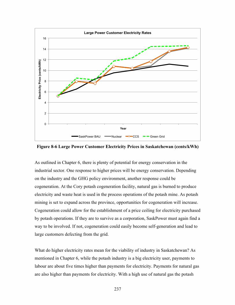
237

Figure 8-6 Large Power Customer Electricity Prices in Saskatchewan (cents/kWh)

As outlined in Chapter 6, there is plenty of potential for energy conservation in the

industrial sector. One response to higher prices will be energy conservation. Depending

on the industry and the GHG policy environment, another response could be

cogeneration. At the Cory potash cogeneration facility, natural gas is burned to produce

electricity and waste heat is used in the process operations of the potash mine. As potash

mining is set to expand across the province, opportunities for cogeneration will increase.

Cogeneration could allow for the establishment of a price ceiling for electricity purchased

by potash operations. If they are to survive as a corporation, SaskPower must again find a

way to be involved. If not, cogeneration could easily become self-generation and lead to

large customers defecting from the grid.

What do higher electricity rates mean for the viability of industry in Saskatchewan? As

mentioned in Chapter 6, while the potash industry is a big electricity user, payments to

labour are about five times higher than payments for electricity. Payments for natural gas

are also higher than payments for electricity. With a high use of natural gas the potash

0

2

4

6

8

10

12

14

16 E

lect

rici

ty P

rice

(cen

ts/k

Wh)

Year

Large Power Customer Electricity Rates

SaskPower BAU Nuclear CCS Green Grid

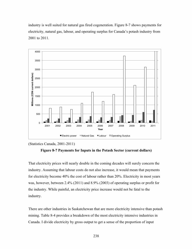
238

industry is well suited for natural gas fired cogeneration. Figure 8-7 shows payments for

electricity, natural gas, labour, and operating surplus for Canada’s potash industry from

2001 to 2011.

(Statistics Canada, 2001-2011)

Figure 8-7 Payments for Inputs in the Potash Sector (current dollars)

That electricity prices will nearly double in the coming decades will surely concern the

industry. Assuming that labour costs do not also increase, it would mean that payments

for electricity become 40% the cost of labour rather than 20%. Electricity in most years

was, however, between 2.4% (2011) and 8.9% (2003) of operating surplus or profit for

the industry. While painful, an electricity price increase would not be fatal to the

industry.

There are other industries in Saskatchewan that are more electricity intensive than potash

mining. Table 8-4 provides a breakdown of the most electricity intensive industries in

Canada. I divide electricity by gross output to get a sense of the proportion of input

0

500

1000

1500

2000

2500

3000

3500

4000

2001 2002 2003 2004 2005 2006 2007 2008 2009 2010 2011

Mill

ions

(CD

N c

urre

nt d

olla

rs)

Year

Electric power Natural Gas Labour Operating Surplus

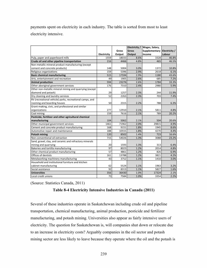
239

payments spent on electricity in each industry. The table is sorted from most to least

electricity intensive.

(Source: Statistics Canada, 2011)

Table 8-4 Electricity Intensive Industries in Canada (2011)

Several of these industries operate in Saskatchewan including crude oil and pipeline

transportation, chemical manufacturing, animal production, pesticide and fertilizer

manufacturing, and potash mining. Universities also appear as fairly intensive users of

electricity. The question for Saskatchewan is, will companies shut down or relocate due

to an increase in electricity costs? Arguably companies in the oil sector and potash

mining sector are less likely to leave because they operate where the oil and the potash is

ElectricityGrossOutput

Electricity/GrossOutput

Wages,Salary,SupplementaryIncome

Electricity/Labour

Pulp,paperandpaperboardmills 1559 18033 8.6% 3328 46.8%Crudeoilandotherpipelinetransportation 216 4466 4.8% 465 46.5%Non-metallicmineralproductmanufacturing(exceptcementandconcreteproducts) 148 5004 3.0% 1372 10.8%Religiousorganizations 159 5396 2.9% 2618 6.1%Basicchemicalmanufacturing 515 17594 2.9% 1180 43.6%Arts,entertainmentandrecreation 49 1905 2.6% 685 7.2%Animalproduction 594 23276 2.6% 1784 33.3%Otheraboriginalgovernmentservices 176 7310 2.4% 2980 5.9%Othernon-metallicmineralminingandquarrying(exceptdiamondandpotash) 29 1257 2.3% 244 11.9%Drycleaningandlaundryservices 52 2263 2.3% 703 7.4%RV(recreationalvehicle)parks,recreationalcamps,androomingandboardinghouses 50 2315 2.2% 788 6.3%Grant-making,civic,andprofessionalandsimilarorganizations 277 12910 2.1% 5811 4.8%Coalmining 159 7616 2.1% 789 20.2%Pesticide,fertilizerandotheragriculturalchemicalmanufacturing 104 5062 2.1% 504 20.6%Othermunicipalgovernmentservices 1461 71962 2.0% 29815 4.9%Cementandconcreteproductmanufacturing 168 9151 1.8% 1945 8.6%Automotiverepairandmaintenance 188 10555 1.8% 4270 4.4%Potashmining 120 8502 1.4% 723 16.6%Non-conventionaloilextraction 715 54026 1.3% 3088 23.2%Sand,gravel,clay,andceramicandrefractorymineralsminingandquarrying 20 1593 1.3% 313 6.4%Bakeriesandtortillamanufacturing 97 8023 1.2% 2014 4.8%Otherchemicalproductmanufacturing 57 4861 1.2% 826 6.9%Officesofdentists 161 13788 1.2% 3821 4.2%Metalworkingmachinerymanufacturing 43 3752 1.1% 1410 3.0%Householdandinstitutionalfurnitureandkitchencabinetmanufacturing 62 5524 1.1% 1963 3.2%Socialassistance 92 8313 1.1% 5827 1.6%Universities 356 36430 1.0% 17324 2.1%Localcreditunions 73 7584 1.0% 3354 2.2%

240

located. In industries like chemical manufacturing, however, companies may relocate to

locations where electricity is less expensive (Interview 5).

The impact of rate increases will also depend on whether an industry is trade-exposed.

Trade-exposed industries compete in international markets and cannot pass costs along to

their customers. A good example of a trade-exposed company is the Evraz Steel mill

operating in Regina, Saskatchewan. In their 2014 submission to the Saskatchewan Rate

Review Panel (SRRP) – the body that arbitrates decisions about utility rates for

Saskatchewan crown corporations – Evraz laid out their circumstances,

EVRAZ Regina Steel is the largest steel company in Western Canada. It is

also one of the largest private sector employers in Regina with 1200

employees and spends over $135 million per year on local purchases of

goods and services.

The steel industry operates in a highly competitive market on a regional,

North American Continent and global level. We currently face stiff

competition from domestic producers and imported product from

international steel companies. The Regina facility also competes with other

EVRAZ global production facilities for investment capital which is based

on earnings and return on investment. This requires the Regina plant to

maximize operational efficiency and minimize costs on an on-going basis.

Our manufacturing processes are highly energy intensive. Next to raw

materials, electricity costs are the next highest cost in producing our steel.

As a result of competitive pressures, increases in power costs cannot be

passed on to our customers. Consequently, increases in power costs have a

direct impact on our bottom line. The EVRAZ Regina location has had a

freight advantage in the northern part of the continent, which has kept us

competitive against other steel companies in North America and globally.

However, this advantage is being eroded by past increases in power costs.

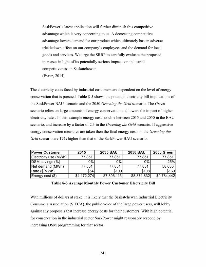
241

SaskPower’s latest application will further diminish this competitive

advantage which is very concerning to us. A decreasing competitive

advantage lowers demand for our product which ultimately has an adverse

trickledown effect on our company’s employees and the demand for local

goods and services. We urge the SRRP to carefully evaluate the proposed

increases in light of its potentially serious impacts on industrial

competitiveness in Saskatchewan.

(Evraz, 2014)

The electricity costs faced by industrial customers are dependent on the level of energy

conservation that is pursued. Table 8-5 shows the potential electricity bill implications of

the SaskPower BAU scenario and the 2050 Greening the Grid scenario. The Green

scenario relies on large amounts of energy conservation and lowers the impact of higher

electricity rates. In this example energy costs double between 2015 and 2050 in the BAU

scenario, and increase by a factor of 2.3 in the Greening the Grid scenario. If aggressive

energy conservation measures are taken then the final energy costs in the Greening the

Grid scenario are 17% higher than that of the SaskPower BAU scenario.

Table 8-5 Average Monthly Power Customer Electricity Bill

With millions of dollars at stake, it is likely that the Saskatchewan Industrial Electricity

Consumers Association (SIECA), the public voice of the large power users, will lobby

against any proposals that increase energy costs for their customers. With high potential

for conservation in the industrial sector SaskPower might reasonably respond by

increasing DSM programming for that sector.

Power Customer 2015 2035 BAU 2050 BAU 2050 GreenElectricity use (MWh) 77,851 77,851 77,851 77,851 DSM savings (%) 0% 0% 0% 25%Net demand (MWh) 77,851 77,851 77,851 58,030 Rate ($/MWh) $54 $100 $108 $169Energy cost ($) $4,172,274 $7,806,115 $8,371,832 $9,784,442

242

Employment Impacts

There have been a number of studies into the employment implications of expanding

renewable energy production. Often these studies are conducted in the context of a

specific policy proposal such as Ontario’s Green Energy and Economy Act and related

feed-in-tariff for renewable electricity. The outcomes of these studies are related to the

methodological approach (and embedded ideology) applied to the analysis (see Winfield

and Dolter, 2014).

Studies that use a Leontief multiplier analysis show that jobs will increase when

increasing renewable energy investment (e.g. Pollin and Garrett-Peltier, 2009). The

Leontief approach measures the direct jobs that result from manufacturing, installing,

operating and maintaining renewable energy facilities. It also measures the indirect jobs

that are associated with the production of intermediate inputs to the manufacture of

renewables, as well as the inputs to those manufacturing processes, and the inputs to

those, and so on. A Leontief analysis documents the entire chain of economic activity that

must occur in order for renewable technologies to be built and installed. Using a

multiplier approach these studies show that the jobs total exceeds the direct jobs created

(for a good review of Leontief analysis see Miller and Blair, 2009).

There are two things missing from a Leontief analysis. The first is an acknowledgement

that if a renewable electricity pathway costs more than a business-as-usual pathway then

the higher electricity prices can reduce economic activity. Money spent on paying for

electricity will be diverted away from investment and consumption in other sectors of the

economy. Böhringer et al. (2012) used CGE modelling to predict a net increase in

unemployment resulting from Ontario’s feed-in-tariff for renewable energy. Hillebrand et

al. (2006) use an econometric model to study Germany’s feed-in-tariff. They find that the

initial investment into renewable energy generates new jobs, but the impact of higher

prices reduces jobs in later years. In total, Hillebrand (2006) forecast a net job loss of

6000 by 2010 due to the German feed-in-tariff.

243

In papers published afterwards, Böhringer and Rivers independently point out that the

employment effects of a feed-in-tariff for renewables will depend on factors like the level

of the subsidy (Böhringer et al., 2013) the mobility of capital (Rivers, 2014), and the

share of labour costs in the production of renewable energy (Rivers, 2014). Rivers (2014)

concludes that renewable energy subsidies like a feed-in-tariff can create jobs “when the

elasticity of substitution between capital and labor is low, when capital is not mobile

internationally, and when the labor intensity of renewable generation is high relative to

conventional generation” (p. 1). He goes on to say that in any case the impact on

employment is “very small” and “the focus of debate around such policies should shift

from employment impacts to other more relevant metrics” (Rivers, 2014: 18).

The second thing missing from a Leontief analysis is a sense of the counter-factual; how

many jobs would have been created by meeting electricity demand in another manner?

What if more natural gas plants had been built instead of more wind turbines? What if

more had been spent on energy conservation? Jobs are created any time money is spent

on investment and new business activity. Of interest to Saskatchewan is the question,

how many jobs are created in the province for each electricity pathway?

Wei et al. (2010) provide some numbers to help answer that question. They conduct a

meta-analysis of job studies to understand the jobs created by investing in various

electricity generation technologies. The job numbers provided by Wei et al. (2010)

include jobs generated in the construction, installation and manufacturing of the

technologies, the operations and maintenance of facilities, and fuel processing for

technologies like natural gas-fired and coal-fired generation. The job calculations are

converted to a measure of job-years per GWh electricity by considering the capacity

factors and expected lifetime of each technology. I revise the Wei et al. (2010) numbers

using the capacity factors and expected lifetime values from SIM. The resulting job

multipliers are presented in Table 8-6. I then use these factors to analyze the seven

scenarios presented in Chapter 7. The results for each time-step are presented in Table 8-

7.

244

Table 8-6 Job Multiplier Factors

Solar photovoltaics stand out in Table 8-6 as the largest job creator per GWh electricity

generated. This is for three reasons, one positive and two less so. The first is that

installing solar photovoltaics is labour-intensive. This means that labour costs are a

higher proportion of total costs. The second, and a less positive reason, is because solar is

more expensive and so more investment is needed to install each megawatt. The third

reason is because solar has a capacity factor of 16% in Saskatchewan, which requires

more megawatts to be installed to generate the same amount of electricity as other

technologies (Croucher, 2011). On these last two points, it is useful to remember that,

while job creation makes for good politics, labour is also a cost of production. The same

can be said for coal and natural gas fired plants equipped with CCS. The CCS process

adds additional jobs and additional costs to generation from those technologies.

I assume that energy conservation creates .15 job-years/GWh saved. Typically, energy

conservation job creation numbers are much higher. The higher numbers come, in large

part, from induced employment. These are jobs in other sectors that result when

electricity customers save money by conserving electricity and then spend it elsewhere in

the economy. Since customers will be paying more for electricity, without conservation

these induced effects will be negative; customers will have less money to spend

elsewhere. Since I do not count the lost spending due to higher prices, I truncate the

conservation job numbers and do not include induced effects from energy conservation.

Generation TechnologyJob-years/

GWhBiomass 0.23Coal 0.14Coal CCS 0.36Natural gas combined cycle 0.12Natural gas simple cycle (peaking) 0.12Natural gas CCS 0.35Hydro 0.26Wind 0.18Solar - Photovoltaic 1.26Small Modular Nuclear Reactor 0.18Conservation 0.15Electricity Storage Capacity 0.15Adapted from Wei et al. (2010)

245

The values in Table 8-6 assume static job multipliers, which is a limitation of the input-

output approach (Lambert and Silva, 2012). We should expect these multipliers to

change. For example, as solar costs decline over time, labour costs and job multipliers

will fall. The multipliers also include manufacturing and indirect jobs created in the

manufacturing process, which might not be representative of jobs created in

Saskatchewan. Currently, Saskatchewan is home to a Hitachi plant, which manufactures

power generation equipment that is used within the province, including the turbine and

generator used for the Boundary Dam CCS facility (Hitachi, 2011) (See Figure 8-8).

(Source: Waldner, 2014)

Figure 8-8 Inside the Hitachi Manufacturing Plant

Whether Saskatchewan will be an attractive place to manufacture other power generation

equipment remains to be seen. Within Canada, Ontario has the first-mover advantage.

The Green Energy and Economy Act – including the local content requirement, which

was subsequently struck down by the World Trade Organization (WTO) – helped Ontario

develop a renewable energy manufacturing base in the province. This makes it more

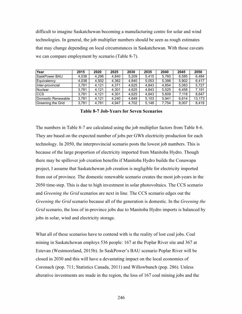
246

difficult to imagine Saskatchewan becoming a manufacturing centre for solar and wind

technologies. In general, the job multiplier numbers should be seen as rough estimates

that may change depending on local circumstances in Saskatchewan. With those caveats

we can compare employment by scenario (Table 8-7).

Table 8-7 Job-Years for Seven Scenarios

The numbers in Table 8-7 are calculated using the job multiplier factors from Table 8-6.

They are based on the expected number of jobs per GWh electricity production for each

technology. In 2050, the interprovincial scenario posts the lowest job numbers. This is

because of the large proportion of electricity imported from Manitoba Hydro. Though

there may be spillover job creation benefits if Manitoba Hydro builds the Conawapa

project, I assume that Saskatchewan job creation is negligible for electricity imported

from out of province. The domestic renewable scenario creates the most job-years in the

2050 time-step. This is due to high investment in solar photovoltaics. The CCS scenario

and Greening the Grid scenarios are next in line. The CCS scenario edges out the

Greening the Grid scenario because all of the generation is domestic. In the Greening the

Grid scenario, the loss of in-province jobs due to Manitoba Hydro imports is balanced by

jobs in solar, wind and electricity storage.

What all of these scenarios have to contend with is the reality of lost coal jobs. Coal

mining in Saskatchewan employs 536 people: 167 at the Poplar River site and 367 at

Estevan (Westmoreland, 2015b). In SaskPower’s BAU scenario Poplar River will be

closed in 2030 and this will have a devastating impact on the local economies of

Coronach (pop. 711; Statistics Canada, 2011) and Willowbunch (pop. 286). Unless

alterative investments are made in the region, the loss of 167 coal mining jobs and the

Year 2015 2020 2025 2030 2035 2040 2045 2050SaskPower BAU 4,038 4,296 4,840 5,209 5,415 5,760 6,585 6,484 Equivalency 4,038 4,502 4,362 4,840 5,053 5,398 5,902 6,417 Inter-provincial 3,781 4,121 4,371 4,625 4,843 4,854 5,083 5,727 Nuclear 3,781 4,121 4,301 4,625 4,843 5,525 6,458 7,191 CCS 3,781 4,121 4,301 4,625 4,843 5,609 7,118 8,647 Domestic Renewable 3,781 4,121 4,240 4,649 5,103 5,941 6,614 13,173 Greening the Grid 3,781 4,781 4,947 4,702 5,148 7,754 8,007 8,419

247

130 employees at the Poplar River plant will send this region into the downward spiral

that characterizes much of rural Saskatchewan.

Many of the coal-related jobs at Estevan (pop. 11,000, Statistics Canada, 2011) would be

protected if the coal-fired plants were retrofit with CCS. This is the plan for Boundary

Dam units IV and V in the SaskPower BAU scenario. Shand will continue operating out

to 2045 as a conventional coal plant and may be retrofit at that time to comply with the

federal coal-fired regulation.

The alternative pathways do not involve coal-fired plants with CCS. Even the scenario I

have called the ‘CCS scenario’ relies on natural gas plants with CCS in order reduce

GHG emissions; coal is phased out when Shand closes in 2045. These alternative

scenarios may be viewed as a threat to the coal mining regions of Estevan/Bienfait and

Coronach/Willowbunch.

Yet Table 8-7 shows that there are employment opportunities in all of the scenarios. The

question is, will the coal miners find work, close to home, building and operating another

electricity generation technology? Strategic planning could make this possible. Estevan is

the sunniest place in the province (and one of the sunniest in Canada) and strategic

investment in a Greening the Grid scenario could shift the workforce away from coal and

towards solar. This would be as much a cultural shift as a technological shift. Coal

mining has a long history in the province and has helped to form the identity of the

southeast region.74

Environmental Impacts

The goal of this dissertation has been to understand pathways to reduce GHG emissions

in the Saskatchewan electricity sector. The seven scenarios outlined in Chapter 7 provide

74 In an historic event in 1931, coal miners were protesting for the right to form a union of their choice. The RCMP opened fire on a union rally in Estevan killing three and wounding many others. A monument to the miners was erected in Bienfait that reads “Lest We Forget. Murdered in Estevan, Sept 29, 1931 by RCMP”. The monument still remains, as does the proud coal culture of the region (Endicott, 2002).

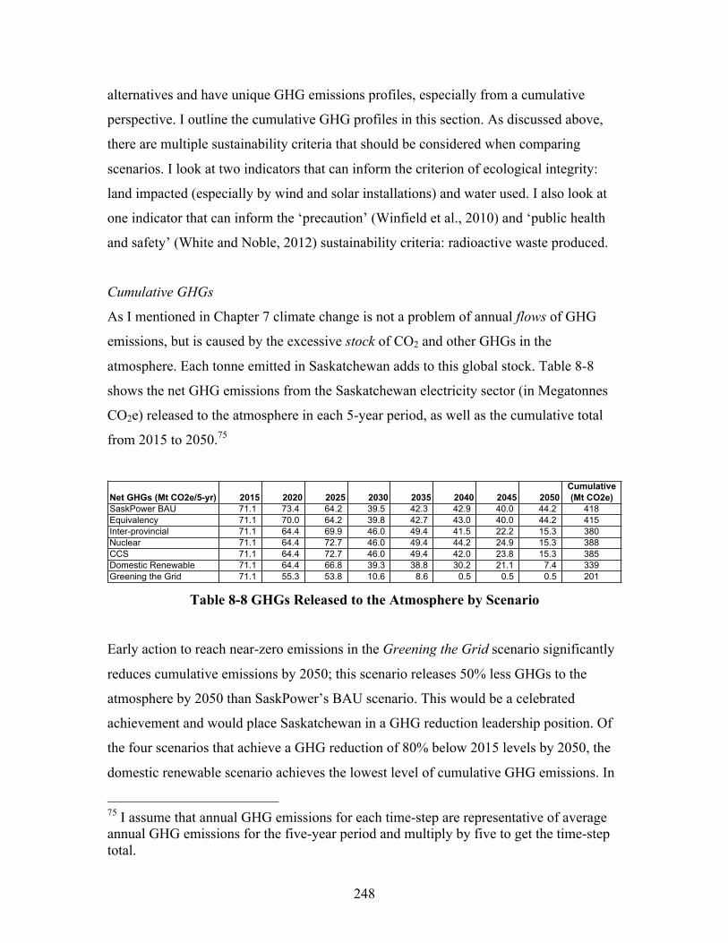
248

alternatives and have unique GHG emissions profiles, especially from a cumulative

perspective. I outline the cumulative GHG profiles in this section. As discussed above,

there are multiple sustainability criteria that should be considered when comparing

scenarios. I look at two indicators that can inform the criterion of ecological integrity:

land impacted (especially by wind and solar installations) and water used. I also look at

one indicator that can inform the ‘precaution’ (Winfield et al., 2010) and ‘public health

and safety’ (White and Noble, 2012) sustainability criteria: radioactive waste produced.

Cumulative GHGs

As I mentioned in Chapter 7 climate change is not a problem of annual flows of GHG

emissions, but is caused by the excessive stock of CO2 and other GHGs in the

atmosphere. Each tonne emitted in Saskatchewan adds to this global stock. Table 8-8

shows the net GHG emissions from the Saskatchewan electricity sector (in Megatonnes

CO2e) released to the atmosphere in each 5-year period, as well as the cumulative total

from 2015 to 2050.75

Table 8-8 GHGs Released to the Atmosphere by Scenario

Early action to reach near-zero emissions in the Greening the Grid scenario significantly

reduces cumulative emissions by 2050; this scenario releases 50% less GHGs to the

atmosphere by 2050 than SaskPower’s BAU scenario. This would be a celebrated

achievement and would place Saskatchewan in a GHG reduction leadership position. Of

the four scenarios that achieve a GHG reduction of 80% below 2015 levels by 2050, the

domestic renewable scenario achieves the lowest level of cumulative GHG emissions. In

75 I assume that annual GHG emissions for each time-step are representative of average annual GHG emissions for the five-year period and multiply by five to get the time-step total.

Net GHGs (Mt CO2e/5-yr) 2015 2020 2025 2030 2035 2040 2045 2050Cumulative (Mt CO2e)

SaskPower BAU 71.1 73.4 64.2 39.5 42.3 42.9 40.0 44.2 418Equivalency 71.1 70.0 64.2 39.8 42.7 43.0 40.0 44.2 415Inter-provincial 71.1 64.4 69.9 46.0 49.4 41.5 22.2 15.3 380Nuclear 71.1 64.4 72.7 46.0 49.4 44.2 24.9 15.3 388CCS 71.1 64.4 72.7 46.0 49.4 42.0 23.8 15.3 385Domestic Renewable 71.1 64.4 66.8 39.3 38.8 30.2 21.1 7.4 339Greening the Grid 71.1 55.3 53.8 10.6 8.6 0.5 0.5 0.5 201

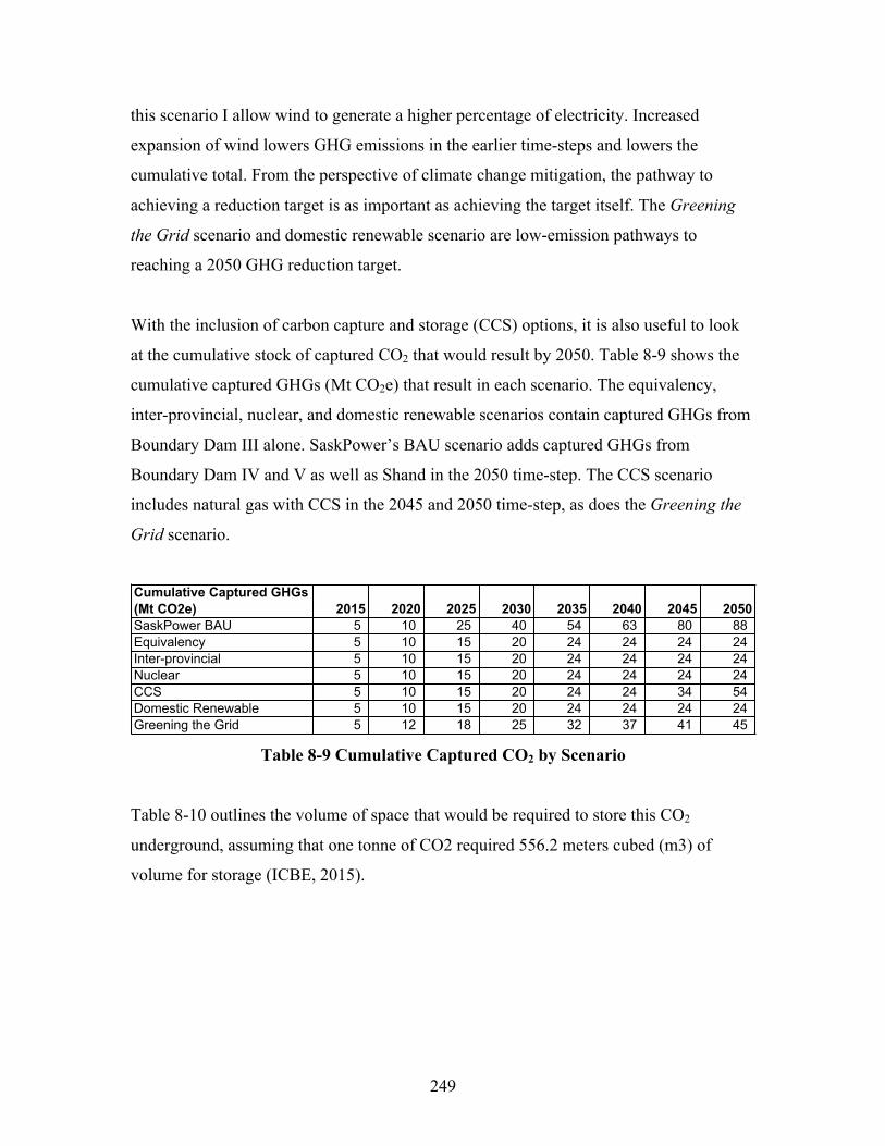
249

this scenario I allow wind to generate a higher percentage of electricity. Increased

expansion of wind lowers GHG emissions in the earlier time-steps and lowers the

cumulative total. From the perspective of climate change mitigation, the pathway to

achieving a reduction target is as important as achieving the target itself. The Greening

the Grid scenario and domestic renewable scenario are low-emission pathways to

reaching a 2050 GHG reduction target.

With the inclusion of carbon capture and storage (CCS) options, it is also useful to look

at the cumulative stock of captured CO2 that would result by 2050. Table 8-9 shows the

cumulative captured GHGs (Mt CO2e) that result in each scenario. The equivalency,

inter-provincial, nuclear, and domestic renewable scenarios contain captured GHGs from

Boundary Dam III alone. SaskPower’s BAU scenario adds captured GHGs from

Boundary Dam IV and V as well as Shand in the 2050 time-step. The CCS scenario

includes natural gas with CCS in the 2045 and 2050 time-step, as does the Greening the

Grid scenario.

Table 8-9 Cumulative Captured CO2 by Scenario

Table 8-10 outlines the volume of space that would be required to store this CO2

underground, assuming that one tonne of CO2 required 556.2 meters cubed (m3) of

volume for storage (ICBE, 2015).

Cumulative Captured GHGs (Mt CO2e) 2015 2020 2025 2030 2035 2040 2045 2050SaskPower BAU 5 10 25 40 54 63 80 88 Equivalency 5 10 15 20 24 24 24 24 Inter-provincial 5 10 15 20 24 24 24 24 Nuclear 5 10 15 20 24 24 24 24 CCS 5 10 15 20 24 24 34 54 Domestic Renewable 5 10 15 20 24 24 24 24 Greening the Grid 5 12 18 25 32 37 41 45

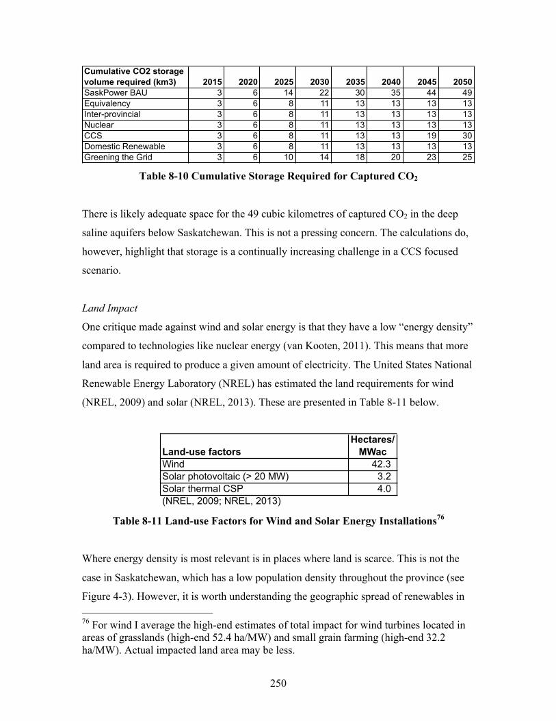
250

Table 8-10 Cumulative Storage Required for Captured CO2

There is likely adequate space for the 49 cubic kilometres of captured CO2 in the deep

saline aquifers below Saskatchewan. This is not a pressing concern. The calculations do,

however, highlight that storage is a continually increasing challenge in a CCS focused

scenario.

Land Impact

One critique made against wind and solar energy is that they have a low “energy density”

compared to technologies like nuclear energy (van Kooten, 2011). This means that more

land area is required to produce a given amount of electricity. The United States National

Renewable Energy Laboratory (NREL) has estimated the land requirements for wind

(NREL, 2009) and solar (NREL, 2013). These are presented in Table 8-11 below.

Table 8-11 Land-use Factors for Wind and Solar Energy Installations76

Where energy density is most relevant is in places where land is scarce. This is not the

case in Saskatchewan, which has a low population density throughout the province (see

Figure 4-3). However, it is worth understanding the geographic spread of renewables in 76 For wind I average the high-end estimates of total impact for wind turbines located in areas of grasslands (high-end 52.4 ha/MW) and small grain farming (high-end 32.2 ha/MW). Actual impacted land area may be less.

Cumulative CO2 storage volume required (km3) 2015 2020 2025 2030 2035 2040 2045 2050SaskPower BAU 3 6 14 22 30 35 44 49Equivalency 3 6 8 11 13 13 13 13Inter-provincial 3 6 8 11 13 13 13 13Nuclear 3 6 8 11 13 13 13 13CCS 3 6 8 11 13 13 19 30Domestic Renewable 3 6 8 11 13 13 13 13Greening the Grid 3 6 10 14 18 20 23 25

Land-use factorsHectares/

MWacWind 42.3 Solar photovoltaic (> 20 MW) 3.2 Solar thermal CSP 4.0 (NREL, 2009; NREL, 2013)

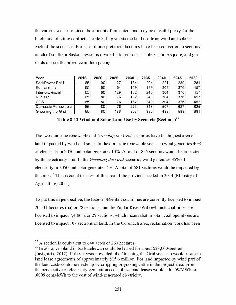
251

the various scenarios since the amount of impacted land may be a useful proxy for the

likelihood of siting conflicts. Table 8-12 presents the land use from wind and solar in

each of the scenarios. For ease of interpretation, hectares have been converted to sections;

much of southern Saskatchewan is divided into sections, 1 mile x 1 mile square, and grid

roads dissect the province at this spacing.

Table 8-12 Wind and Solar Land Use by Scenario (Sections)77

The two domestic renewable and Greening the Grid scenarios have the highest area of

land impacted by wind and solar. In the domestic renewable scenario wind generates 40%

of electricity in 2050 and solar generates 13%. A total of 825 sections would be impacted

by this electricity mix. In the Greening the Grid scenario, wind generates 35% of

electricity in 2050 and solar generates 4%. A total of 681 sections would be impacted by

this mix.78 This is equal to 1.2% of the area of the province seeded in 2014 (Ministry of

Agriculture, 2015).

To put this in perspective, the Estevan/Bienfait coalmines are currently licensed to impact

20,331 hectares (ha) or 78 sections, and the Poplar River/Willowbunch coalmines are

licensed to impact 7,488 ha or 29 sections, which means that in total, coal operations are

licensed to impact 107 sections of land. In the Coronach area, reclamation work has been

77 A section is equivalent to 640 acres or 260 hectares. 78 In 2012, cropland in Saskatchewan could be leased for about $23,000/section (Insightrix, 2012). If these costs prevailed, the Greening the Grid scenario would result in land lease agreements of approximately $15.6 million. For land impacted by wind part of the land costs could be made up by cropping or grazing cattle in the project area. From the perspective of electricity generation costs, these land leases would add .09/MWh or .0009 cents/kWh to the cost of wind-generated electricity.

Year 2015 2020 2025 2030 2035 2040 2045 2050SaskPower BAU 65 90 127 184 204 221 239 281Equivalency 65 65 64 169 189 303 376 457Inter-provincial 65 80 129 182 240 304 376 457Nuclear 65 80 76 182 240 304 376 457CCS 65 80 76 182 240 304 376 457Domestic Renewable 65 80 76 273 348 507 627 825Greening the Grid 65 80 186 303 385 488 588 681

252

done to restore impacted land back to agricultural quality (Interview 19). In the Estevan

area there are still old coalmines in need of reclamation (Interview 19).

It should be noted that measures of land impacted by wind and solar consist of direct

impacts associated with physical infrastructure such as roads, turbines, solar arrays,

transmission lines, as well land that is indirectly associated with the project area. Direct

land impacts are about 1/100th of the total impacted land area for wind (NREL, 2009).

Turbines are 10% of that total (or 1/1000th), while roads make up 79% of the direct

impacts of wind (NREL, 2009). This means that much of the impacted land is still

available for cropping or grazing. This agricultural activity just so happens to occur in the

midst of a wind farm.

Water Impact

Saskatchewan is a semi-arid region. Drought is always a threat and water is precious. As

mentioned in Chapter 4, drought has impacted the coal-fired electricity sector in the past

(Maathuis and van der Kamp, 2011). Table 8-13 shows the water requirements of the

electricity generation technologies included in my analysis. These indicators are the

median values for each technology in a 2011 NREL study (NREL, 2011). Nuclear power

plants and natural gas combined cycle plants are the greatest water users. Hydroelectric

facilities (which use water and then release it downstream) also have large water

requirements.

I use these indicators to analyze the water impacts of the seven scenarios from Chapter 7.

The results are presented in Table 8-14 in terms of Gigalitres per year (billion litres per

year) and in Table 8-15 in terms of thousands of Olympic sized swimming pools (a

perhaps more intuitive figure; each Olympic swimming pool contains 2.5 Megalitres of

water).

253

Table 8-13 Water Impact Indicators

As a word of caution, these water impacts include consumption and withdrawals, but they

do not indicate changes in water quality. Ontario’s nuclear plants routinely release tritium

into Lake Ontario (Winfield et al., 2006). Tables 8-14 and 8-15 do not capture this

qualitative impact on water. These figures also only include direct water impacts. The

water impact of coal mining, natural gas extraction, and uranium mining is not included,

and neither is the water impact of manufacturing processes required to create the

electricity generation equipment. This means these numbers are an incomplete measure

of water impact, but they are a useful measure of drought resilience. They can be used to

determine, once a given scenario is in place, how vulnerable it is to drought conditions.

Table 8-14 Water Impact by Scenario (Gigalitres/yr)

Generation TechnologyBiomassCoal

Coal CCSNatural gas combined cycleNatural gas simple cycle (peaking)

Natural gas CCS

HydroWindSolar - PhotovoltaicSolar - Thermal CSPSmall Modular Nuclear ReactorConservationElectricity Storage CapacitySource: NREL (2011)

Type

Water Consumption

(L/MWh)

Water Withdrawals

(L/MWh)Total

(L/MWh)Steam pond 1,476 1,703 3,180 Generic pond 2,063 2,063 subcritical with

CCS 3,202 3,202 Pond 908 22,523 23,432 Pond 908 22,523 23,432

Tower combined cycle with CCS 1,431 1,878 3,308 Aggregated In-

stream and Reservoir 17,000 17,000

0 - 98 98

Trough dry 295 295 Pond 26,687 26,687

- -

Water Impact (Gigalitre/yr) 2015 2020 2025 2030 2035 2040 2045 2050SaskPower BAU 295 334 366 464 500 543 600 668Equivalency 303 325 363 458 494 501 592 590Inter-provincial 285 326 397 471 515 506 484 481Nuclear 285 326 429 471 515 517 526 552CCS 285 326 429 471 515 490 419 333Domestic Renewable 285 326 471 508 532 467 392 253Greening the Grid 285 277 292 349 343 289 288 289

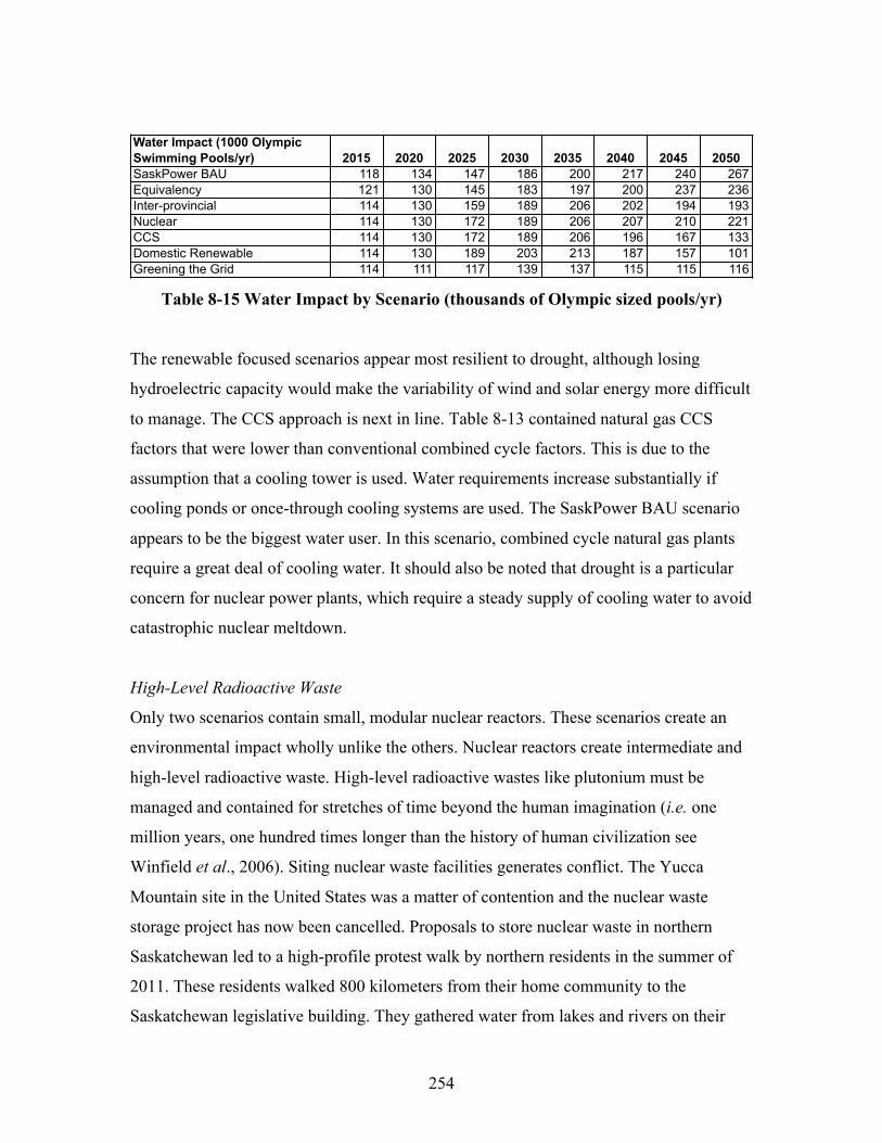
254

Table 8-15 Water Impact by Scenario (thousands of Olympic sized pools/yr)

The renewable focused scenarios appear most resilient to drought, although losing

hydroelectric capacity would make the variability of wind and solar energy more difficult

to manage. The CCS approach is next in line. Table 8-13 contained natural gas CCS

factors that were lower than conventional combined cycle factors. This is due to the

assumption that a cooling tower is used. Water requirements increase substantially if

cooling ponds or once-through cooling systems are used. The SaskPower BAU scenario

appears to be the biggest water user. In this scenario, combined cycle natural gas plants

require a great deal of cooling water. It should also be noted that drought is a particular

concern for nuclear power plants, which require a steady supply of cooling water to avoid

catastrophic nuclear meltdown.

High-Level Radioactive Waste

Only two scenarios contain small, modular nuclear reactors. These scenarios create an

environmental impact wholly unlike the others. Nuclear reactors create intermediate and

high-level radioactive waste. High-level radioactive wastes like plutonium must be

managed and contained for stretches of time beyond the human imagination (i.e. one

million years, one hundred times longer than the history of human civilization see

Winfield et al., 2006). Siting nuclear waste facilities generates conflict. The Yucca

Mountain site in the United States was a matter of contention and the nuclear waste

storage project has now been cancelled. Proposals to store nuclear waste in northern

Saskatchewan led to a high-profile protest walk by northern residents in the summer of

2011. These residents walked 800 kilometers from their home community to the

Saskatchewan legislative building. They gathered water from lakes and rivers on their

Water Impact (1000 Olympic Swimming Pools/yr) 2015 2020 2025 2030 2035 2040 2045 2050SaskPower BAU 118 134 147 186 200 217 240 267Equivalency 121 130 145 183 197 200 237 236Inter-provincial 114 130 159 189 206 202 194 193Nuclear 114 130 172 189 206 207 210 221CCS 114 130 172 189 206 196 167 133Domestic Renewable 114 130 189 203 213 187 157 101Greening the Grid 114 111 117 139 137 115 115 116

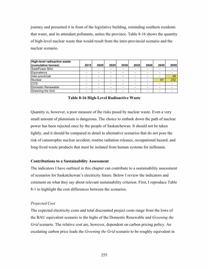
255

journey and presented it in front of the legislative building, reminding southern residents

that water, and its attendant pollutants, unites the province. Table 8-16 shows the quantity

of high-level nuclear waste that would result from the inter-provincial scenario and the

nuclear scenario.

Table 8-16 High-Level Radioactive Waste

Quantity is, however, a poor measure of the risks posed by nuclear waste. Even a very

small amount of plutonium is dangerous. The choice to embark down the path of nuclear

power has been rejected once by the people of Saskatchewan. It should not be taken

lightly, and it should be compared in detail to alternative scenarios that do not pose the

risk of catastrophic nuclear accident, routine radiation releases, occupational hazard, and

long-lived waste products that must be isolated from human systems for millennia.

Contributions to a Sustainability Assessment

The indicators I have outlined in this chapter can contribute to a sustainability assessment

of scenarios for Saskatchewan’s electricity future. Below I review the indicators and

comment on what they say about relevant sustainability criterion. First, I reproduce Table

8-1 to highlight the cost differences between the scenarios.

Projected Cost

The expected electricity costs and total discounted project costs range from the lows of

the BAU equivalent scenario to the highs of the Domestic Renewable and Greening the

Grid scenario. The relative cost are, however, dependent on carbon pricing policy. An

escalating carbon price leads the Greening the Grid scenario to be roughly equivalent in

High-level radioactive waste (cumulative tonnes) 2015 2020 2025 2030 2035 2040 2045 2050SaskPower BAU - - - - - - - - Equivalency - - - - - - - - Inter-provincial - - - - - - - 28 Nuclear - - - - - - 67 232 CCS - - - - - - - - Domestic Renewable - - - - - - - - Greening the Grid - - - - - - - -

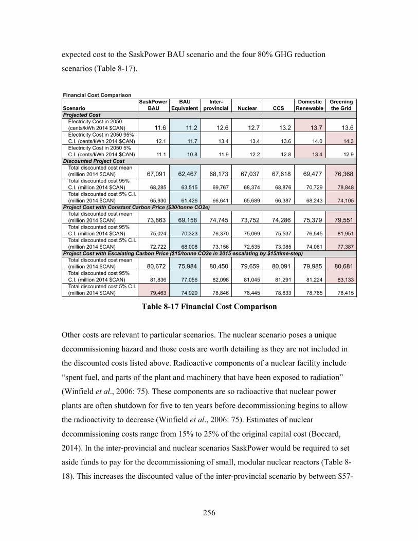
256

expected cost to the SaskPower BAU scenario and the four 80% GHG reduction

scenarios (Table 8-17).

Table 8-17 Financial Cost Comparison

Other costs are relevant to particular scenarios. The nuclear scenario poses a unique

decommissioning hazard and those costs are worth detailing as they are not included in

the discounted costs listed above. Radioactive components of a nuclear facility include

“spent fuel, and parts of the plant and machinery that have been exposed to radiation”

(Winfield et al., 2006: 75). These components are so radioactive that nuclear power

plants are often shutdown for five to ten years before decommissioning begins to allow

the radioactivity to decrease (Winfield et al., 2006: 75). Estimates of nuclear

decommissioning costs range from 15% to 25% of the original capital cost (Boccard,

2014). In the inter-provincial and nuclear scenarios SaskPower would be required to set

aside funds to pay for the decommissioning of small, modular nuclear reactors (Table 8-

18). This increases the discounted value of the inter-provincial scenario by between $57-

Financial Cost Comparison

ScenarioSaskPower

BAU BAU

EquivalentInter-

provincial Nuclear CCSDomestic

RenewableGreening the Grid

Electricity Cost in 2050 (cents/kWh 2014 $CAN) 11.6 11.2 12.6 12.7 13.2 13.7 13.6 Electricity Cost in 2050 95% C.I. (cents/kWh 2014 $CAN) 12.1 11.7 13.4 13.4 13.6 14.0 14.3 Electricity Cost in 2050 5% C.I. (cents/kWh 2014 $CAN) 11.1 10.8 11.9 12.2 12.8 13.4 12.9

Total discounted cost mean (million 2014 $CAN) 67,091 62,467 68,173 67,037 67,618 69,477 76,368 Total discounted cost 95% C.I. (million 2014 $CAN) 68,285 63,515 69,767 68,374 68,876 70,729 78,848 Total discounted cost 5% C.I. (million 2014 $CAN) 65,930 61,426 66,641 65,689 66,387 68,243 74,105

Total discounted cost mean (million 2014 $CAN) 73,863 69,158 74,745 73,752 74,286 75,379 79,551 Total discounted cost 95% C.I. (million 2014 $CAN) 75,024 70,323 76,370 75,069 75,537 76,545 81,951 Total discounted cost 5% C.I. (million 2014 $CAN) 72,722 68,008 73,156 72,535 73,085 74,061 77,387

Total discounted cost mean (million 2014 $CAN) 80,672 75,984 80,450 79,659 80,091 79,985 80,681 Total discounted cost 95% C.I. (million 2014 $CAN) 81,836 77,056 82,098 81,045 81,291 81,224 83,133 Total discounted cost 5% C.I. (million 2014 $CAN) 79,463 74,929 78,846 78,445 78,833 78,765 78,415

Projected Cost

Discounted Project Cost

Project Cost with Constant Carbon Price ($30/tonne CO2e)

Project Cost with Escalating Carbon Price ($15/tonne CO2e in 2015 escalating by $15/time-step)

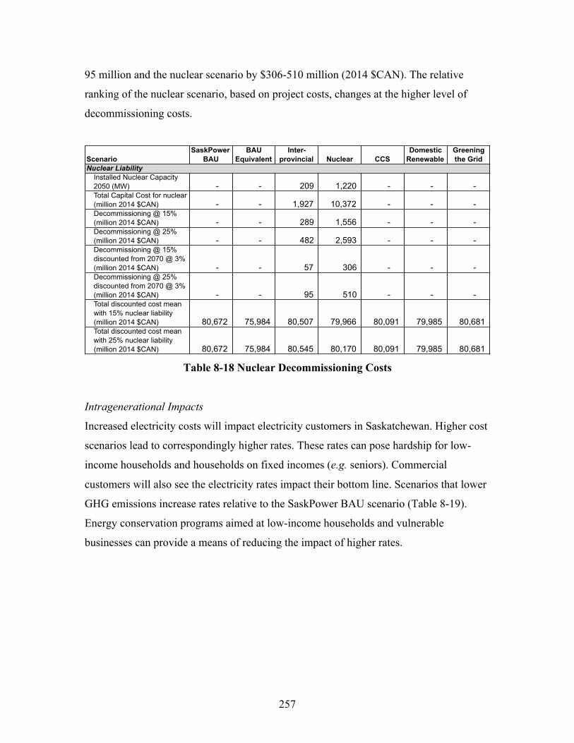
257

95 million and the nuclear scenario by $306-510 million (2014 $CAN). The relative

ranking of the nuclear scenario, based on project costs, changes at the higher level of

decommissioning costs.

Table 8-18 Nuclear Decommissioning Costs

Intragenerational Impacts

Increased electricity costs will impact electricity customers in Saskatchewan. Higher cost

scenarios lead to correspondingly higher rates. These rates can pose hardship for low-

income households and households on fixed incomes (e.g. seniors). Commercial

customers will also see the electricity rates impact their bottom line. Scenarios that lower

GHG emissions increase rates relative to the SaskPower BAU scenario (Table 8-19).

Energy conservation programs aimed at low-income households and vulnerable

businesses can provide a means of reducing the impact of higher rates.

ScenarioSaskPower

BAU BAU

EquivalentInter-

provincial Nuclear CCSDomestic

RenewableGreening the Grid

Installed Nuclear Capacity 2050 (MW) - - 209 1,220 - - - Total Capital Cost for nuclear (million 2014 $CAN) - - 1,927 10,372 - - - Decommissioning @ 15% (million 2014 $CAN) - - 289 1,556 - - - Decommissioning @ 25% (million 2014 $CAN) - - 482 2,593 - - - Decommissioning @ 15% discounted from 2070 @ 3% (million 2014 $CAN) - - 57 306 - - - Decommissioning @ 25% discounted from 2070 @ 3% (million 2014 $CAN) - - 95 510 - - - Total discounted cost mean with 15% nuclear liability (million 2014 $CAN) 80,672 75,984 80,507 79,966 80,091 79,985 80,681 Total discounted cost mean with 25% nuclear liability (million 2014 $CAN) 80,672 75,984 80,545 80,170 80,091 79,985 80,681

Nuclear Liability

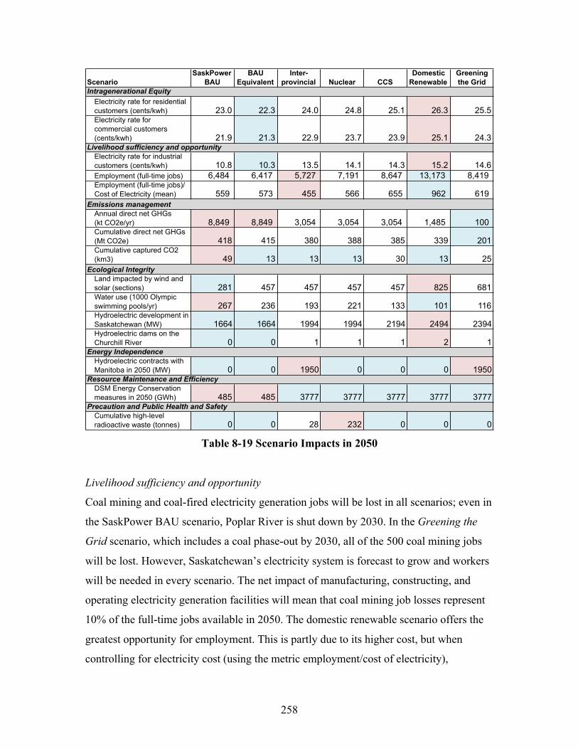
258

Table 8-19 Scenario Impacts in 2050

Livelihood sufficiency and opportunity

Coal mining and coal-fired electricity generation jobs will be lost in all scenarios; even in

the SaskPower BAU scenario, Poplar River is shut down by 2030. In the Greening the

Grid scenario, which includes a coal phase-out by 2030, all of the 500 coal mining jobs

will be lost. However, Saskatchewan’s electricity system is forecast to grow and workers

will be needed in every scenario. The net impact of manufacturing, constructing, and

operating electricity generation facilities will mean that coal mining job losses represent

10% of the full-time jobs available in 2050. The domestic renewable scenario offers the

greatest opportunity for employment. This is partly due to its higher cost, but when

controlling for electricity cost (using the metric employment/cost of electricity),

ScenarioSaskPower

BAU BAU

EquivalentInter-

provincial Nuclear CCSDomestic

RenewableGreening the Grid

Electricity rate for residential customers (cents/kwh) 23.0 22.3 24.0 24.8 25.1 26.3 25.5Electricity rate for commercial customers (cents/kwh) 21.9 21.3 22.9 23.7 23.9 25.1 24.3

Electricity rate for industrial customers (cents/kwh) 10.8 10.3 13.5 14.1 14.3 15.2 14.6Employment (full-time jobs) 6,484 6,417 5,727 7,191 8,647 13,173 8,419 Employment (full-time jobs)/ Cost of Electricity (mean) 559 573 455 566 655 962 619

Annual direct net GHGs (kt CO2e/yr) 8,849 8,849 3,054 3,054 3,054 1,485 100 Cumulative direct net GHGs (Mt CO2e) 418 415 380 388 385 339 201Cumulative captured CO2 (km3) 49 13 13 13 30 13 25

Land impacted by wind and solar (sections) 281 457 457 457 457 825 681Water use (1000 Olympic swimming pools/yr) 267 236 193 221 133 101 116Hydroelectric development in Saskatchewan (MW) 1664 1664 1994 1994 2194 2494 2394Hydroelectric dams on the Churchill River 0 0 1 1 1 2 1

Hydroelectric contracts with Manitoba in 2050 (MW) 0 0 1950 0 0 0 1950

DSM Energy Conservation measures in 2050 (GWh) 485 485 3777 3777 3777 3777 3777

Cumulative high-level radioactive waste (tonnes) 0 0 28 232 0 0 0

Energy Independence

Resource Maintenance and Efficiency

Precaution and Public Health and Safety

Ecological Integrity

Emissions management

Livelihood sufficiency and opportunity

Intragenerational Equity

259

employment is still higher for the domestic renewable scenario. If the province moves

away from coal, the question will be, will the new jobs be available in the same location

as existing jobs? Halliday (2013) suggests a solar thermal plant for the Coronach area to

provide jobs for coal miners and employees at the Poplar River plant. Opportunities to

manufacture components in Saskatchewan would also contribute to employment, but are

in no way guaranteed.

While there will be jobs in the electricity sector, higher electricity rates may lead to job

losses in other sectors. Energy-intensive industries such as chemical manufacturing and

steel manufacturing may choose to leave Saskatchewan for locations with lower rates.

Household and business spending would be redirected from other areas of the economy

towards their electricity bills. The higher the electricity rates, the greater the threat of job

loss throughout the rest of the economy.

Emissions Management

It is a central focus of this dissertation to find electricity scenarios that reduce GHG

emissions. The Greening the Grid scenario achieves near-zero emissions by 2040 (100 kt

CO2e/yr) and maintains this low level of GHG emissions to 2050. This early action leads

to cumulative GHG emissions measuring half that of the SaskPower BAU scenario. In

contrast, action is delayed in the four scenarios that reduce GHGs by 80% by 2050 and

cumulative GHG emission are 137-179 Mt CO2e higher than the Greening the Grid

scenario, nearly approaching that of the SaskPower BAU scenario. Early action would

enhance Saskatchewan’s contribution to global efforts to mitigate climate change. It is

also worth noting that the SaskPower BAU scenario, which relies on converting coal-

fired generation stations to carbon capture and storage (CCS), requires the largest volume

of underground space to store CO2. To those who advocate using captured CO2 for

enhanced oil recovery this may be a benefit of the scenario.

Ecological Integrity

Four indicators can contribute to our understanding of the ecological integrity of each

scenario: land impacted by wind and solar; water use; hydroelectric capacity; and the

260

number of hydroelectric projects on the Churchill River. Land impacted by solar and

wind is highest in the domestic renewable scenario. This indicates a higher potential for

land use conflicts or wildlife impacts. From the perspective of landowners, this also

represents an economic opportunity. Land lease payments for wind turbines are generally

in the range of $8000 per turbine per year (Baxter et al., 2013).

The domestic renewable scenario has the lowest water impact of all scenarios, followed

closely by the Greening the Grid scenario. This makes installed wind and solar facilities

resilient against drought (although their manufacture may not be). Scenarios that rely on

coal-fired generation, natural-gas fired generation, and nuclear generation require the

most water. Without a steady supply of cooling water coal-fired and natural-gas fired

units must shut down. Without cooling water, a nuclear plant could risk a melt-down.

This makes the thermal, and especially nuclear generation facilities, susceptible to

drought.

Further work needs to be done to understand the impacts of drought on hydroelectricity

production. The domestic renewable scenario and Greening the Grid scenario have the

highest reliance on hydroelectricity. This power is needed to balance the variability of

wind and solar. Though wind and solar may be resilient to drought, an energy system

combining wind and solar and hydroelectricity may not be. The Greening the Grid

scenario was designed to meet electricity demand in periods of seasonally low

hydroelectric availability. The possibility of a multi-year mega-drought must also be

examined.

Hydroelectric facilities create lasting ecological impacts by modifying river systems. I

include the number of facilities assumed to be constructed on the Churchill River as a

proxy of hydroelectric impact on ecological integrity. In the late 1970s people rejected

the Wintego project on the Churchill River because of the ecological impacts it would

cause. At the time the Churchill River Board of Inquiry reported that the proposed 300

MW Wintego dam would create,

261

“a new reservoir extending approximately 70 miles upstream from the

Wintego site to Drinking Falls on the Churchill River and extending

upstream on the Reindeer River for the full extent of the river, some 59

miles upstream to Whitesand Dam…The reservoir so created would flood

an additional 112 square miles of land.”

(Churchill River Board of Inquiry (CRBI), 1978: 10)

All of the GHG reduction scenarios assume that a Wintego type project would proceed on

the Churchill River. The domestic renewable scenario assumes that a second

hydroelectric facility would be constructed on the Churchill River. The social

acceptability of these hydroelectric facilities remains in doubt. Opposition to the Wintego

project in the 1970s came from groups ranging from northern First Nations – especially

the Cree peoples who have traditionally lived along the Churchill River – northern Métis

peoples who have connections to the river dating back to the voyageurs who used it as a

key transportation artery for the fur trade, and southern settler groups who value the

recreational opportunities offered by the Churchill. The National and Provincial Parks

Association spoke of the “triple value” of the Churchill: “it’s a wild river, it is scenic, and

it is of historic importance to Canada” (CRBI, 1978: 38). If hydroelectric projects are not

built on the Churchill River additional low-carbon firm capacity must be obtained from

other sources.

The lessons from Cumberland House should also be remembered. If new hydroelectric

projects are used to balance the variability of wind and solar energy, as I have shown

them to be used in Chapter 7, the downstream river flows will be highly erratic. As

recounted in the quote found on page 59, the erratic outflows from the E.B. Campbell

dam created hardship for the people of Cumberland House impacting wildlife, local

outfitting businesses, and the way of life of the people of Cumberland House. Limits on

the operating range of hydroelectric facilities can reduce downstream impacts, but will

also mean that other back-up sources must be brought on-line to balance the variability of

wind and solar power.

262

Energy Independence

Premier Wall has stated that he prefers coal-fired generation with carbon capture and

storage to hydroelectricity imports from Manitoba because coal offers a greater degree of

energy independence (Zinchuk, 2014). Two scenarios include large scale contracts with

Manitoba Hydro in 2050: the inter-provincial scenario and the Greening the Grid

scenario. These scenarios also have the greatest range of uncertainty around their costs.

The risk of relying on Manitoba Hydro electricity is that prices are set outside the

province, and outside of SaskPower’s control. If this risk is to be mitigated, stable long-

term contracts must be signed between SaskPower and Manitoba Hydro.

Some of the 1950 MW of Manitoba Hydro capacity included in the inter-provincial and

Greening the Grid scenarios would come from the Keeyask project. This 695 MW

hydroelectric project is a partnership between Manitoba Hydro and four First Nations. It

is currently under construction. The rest of the capacity from Manitoba Hydro would

require the construction of the Conawapa hydroelectric project. That project is currently

on hold “until more export sales are confirmed” (Puxley, 2014). If Saskatchewan is to

access this power in time to replace the coal-fired plants being retired in 2028 and 2030 it

will have to act soon to sign import agreements with Manitoba Hydro.

Resource Maintenance and Efficiency

Winfield et al. (2010) argue that a sustainable electricity pathway will focus on resource

maintenance and efficiency, including end-use energy efficiency. In all of the GHG

emission reduction scenarios DSM conservation efforts are pursued to the maximum

potential allowed in SIM (3777 GWh in 2050). This stands in contrast to the SaskPower

BAU and BAU equivalency scenarios. The difference is explained by industrial DSM

becoming cost-competitive in scenarios with higher electricity prices.

Precaution, Public health and safety, Extreme Event Risk

All three sets of sustainability criteria proposed at the beginning of this chapter include

mention of something like precaution (Winfield et al., 2010), public health and safety

(White and Noble, 2012), or extreme event risk (Jaccard, 2005). These criteria seem

263

tailored to bring attention to the unique dangers posed by nuclear energy. Nuclear energy

poses an extreme event risk in the form of catastrophic meltdown (e.g. Fukushima). It

poses public health and safety risks through routine and accidental release of radiation

(Winfield et al., 2006). The safety of a nuclear facility is fraught with uncertainty and so

invites the application of the precautionary principle. These risks are enough to

encourage many people – including those who expressed their opposition to nuclear

power at the Perrins’ (2009) consultation meetings – to strike the inter-provincial and

nuclear scenarios off the list of desirable electricity futures.

Path Dependence

Jaccard (2005) and Winfield et al. (2010) both list path dependence as a consideration in

an assessment of electricity futures. For Jaccard (2005) a scenario is more politically

acceptable if it aligns with existing institutions. Path dependence in this instance is

something to recommend a scenario. For Winfield et al. (2010) path dependence is a

potential trap to be avoided. In Ontario, where Winfield et al. (2010) focus their research,

large nuclear plants have been built. The socio-technical apparatus that surrounds these

nuclear plants creates a powerful political lobby for maintaining and expanding nuclear

power in the generation mix. Path dependence in the Ontario electricity system reduces

flexibility and adaptive capacity, limiting future electricity generation options (Winfield

et al., 2010).

Saskatchewan does not have nuclear power plants, but it does have a uranium mining

industry with strong ties to the nuclear power industry (uranium mining company

CAMECO is a part-owner of Ontario’s Bruce Power nuclear power corporation). There is

a strong sense among the business community and leadership of the Saskatchewan Party

that Saskatchewan should build a nuclear power plant. In the UDP (2009) report, nuclear

power was represented as a way to “add value” to Saskatchewan’s uranium. This creates,

if not path dependence, at least path pressure to build a nuclear power plant.

Interest in nuclear power also comes from the International Brotherhood of Electrical

Workers (IBEW) labour union. Neil Collins, then business manager for the IBEW, had a

264

seat on the UDP (2009) panel that recommended Saskatchewan build a nuclear power

plant. The IBEW also signed an agreement with Bruce Power guaranteeing union jobs

were a nuclear power plant to be built. The IBEW continued to show their support during

the Perrins’ (2009) consultations, when at each meeting an IBEW member would stand to

advocate for nuclear power and explain why wind and solar power could not supply

“baseload power.”

In Saskatchewan, where coal has been king since Boundary Dam was commissioned in

1959, path dependence points towards the continued existence of coal-fired electricity.

SaskPower staff and senior management have spent their careers working in a coal-based

electricity system. This familiarity with coal breeds allegiance, and the effect can be

powerful. In Chapter 7 I showed that the GHG emission reductions that will result from

the federal coal-fired regulations could be achieved at a lower cost by allowing coal

facilities to be retired at the end of their useful lives, and replacing them with natural gas

combined cycle plants and wind turbines, instead of converting them to carbon capture

and storage. SaskPower and Premier Brad Wall have other plans. In the Fall of 2015 the

Premier expressed his continued support for the Boundary Dam III carbon capture and

storage plant, despite cost over-runs, and despite the fact that it was still suffering from

problems that kept it from running at full capacity,

“Mr. Speaker, it’s going to get to 90 per cent (carbon capture) on a

consistent basis. We know that in the coming months the plant will be

operational again. And we need it to be operational if we’re going to

continue to have coal, cleaner coal in the fleet, if we’re going to continue

to have coal mining jobs in the province.”

(CBC, 2015e)

Members of the IBEW were also quoted expressing their support for the Premier’s

position on coal (Langenegger, 2015). The large centralized technologies – nuclear and

coal - appear to be a good fit for the IBEW workforce. Path dependence may keep

Saskatchewan on the trail of carbon capture and storage despite the availability of other

options.

265

Conclusions

The scenarios I outlined in Chapter 7 are diverse in their impacts. The SaskPower BAU

scenario posts the second lowest electricity price increases, but the highest cumulative

GHGs, stored GHGs, and water requirements. The Greening the Grid scenario achieves

the lowest cumulative level of GHG emissions, the lowest water requirements, and avoids

nuclear waste, but also increases electricity prices and impacts a large area of land. The

analysis reveals that there is no consequence free pathway to Saskatchewan’s electricity

future. Trade-offs are involved and decisions must be made that balance attributes against

one another. In a qualitative sense, this was the work of White and Noble (2012) who

found a renewable based scenario to be the preferred electricity pathway. Further work

can be done to involve the citizens of Saskatchewan in evaluating trade-offs and deciding

which pathway is best for the province. The information I have presented in this chapter

can inform such a discussion.

It is worth noting the many additional impacts that have not been explored in this chapter.

This list includes:

• Health impacts from fossil fuel emissions like sulphur dioxide and particulate

matter;

• Environmental impacts from sulphur dioxide (e.g. acid deposition in lakes);

• Environmental impacts from mercury released by coal-fired electricity plants;

• Lifecycle environmental impacts from rare-earth elements contained in lithium-

ion batteries (if that storage method is pursued);

• Lifecycle energy requirements for technologies that would indicate the ‘Energy

Return on Investment’ of competing options;

• Land impacts from hydroelectricity dams, natural gas extraction, uranium mining;

• Wildlife impacts; and importantly,

• Climate change costs in Saskatchewan avoided through global GHG reduction.

There are also social impacts associated with the various scenarios that include:

• International reputation from contributing to GHG reduction;

• Community division if controversial technologies such as nuclear are pursued;

266

• Community conflict over the siting of electricity generation technologies;

• Impact of each scenario on Aboriginal Rights.

On this last indicator, the history of electricity development in Saskatchewan has not

been kind to Aboriginal people. The E.B. Campbell dam resulted in significant impacts to

downstream fishers and outfitters, many of who were Métis or First Nation. The First

Nations Power Authority (FNPA) appears to be a step in a better direction. The FNPA

works with First Nations to develop electricity generation projects in Saskatchewan. It

serves as a bridge between SaskPower and First Nations. Already the FNPA has

developed a solar photovoltaic tracking project in Swift Current in partnership with the

File Hills Qu’Appelle Tribal Council, an affiliation of eleven First Nations in the

province (Interview 7). Continued partnership and consultation could help to ensure that

aboriginal rights are respected and the electricity system becomes a vehicle for

supporting aboriginal livelihoods (see Martens, 2015).

267

Chapter 9 – Deliberating Saskatchewan’s Electricity Future

Introduction

In this chapter I outline the results of three deliberative energy policy modelling

workshops. These workshops allowed stakeholders engaged in Saskatchewan electricity

policy to evaluate scenarios for Saskatchewan’s electricity future using an interactive

version of the Saskatchewan Investment Model (iSIM).

The workshops also presented opportunities for stakeholders to meet one another,

exchange views, and, it is hoped, develop a greater understanding of one another’s

positions. Akin to van den Belt’s (2004) Mediated Modeling, the deliberative workshops

are an opportunity to “increase the level of shared understanding amongst the group” (p.

17). This shared understanding can act as a foundation for “investigating policy, research,

or management alternatives” (van den Belt, 2004: 17). Shared understanding is also very

much an end in and of itself. One of the most important outcomes of a deliberative

modelling process is “the growth of mutual recognition and compassion” (Ravetz, 1999:

652).

Models such as iSIM are idealized representations of the world and “useful ways of

disciplining our thinking” when used to support deliberation (Victor, 2015). They provide

opportunities for participants to test their understanding of the Saskatchewan electricity

system against an empirically grounded model of the system. Conversely, they are

intended to allow participants to challenge and improve the manner in which the system

is modelled. In both of these ways the model helps to structure a deliberative discussion

(van den Belt, 2004).

The deliberative modelling workshops build on the work of Richards et al. (2012) who

conducted interviews with sixteen individuals in Saskatchewan on the topic of wind

energy. Richards et al. (2012) found differences in participants’ views on whether the

rate of expansion of wind energy in Saskatchewan was adequate. Those who believed the

pace was adequate cited technological barriers to integrating variable wind energy onto

268

the provincial grid. Those who believed the pace was too slow cited political barriers

such as the lack of carbon pricing, feed-in-tariff, or renewable generation targets.

Richards et al. (2012) theorized “Opposing sides may never agree simply because their

perceptions of barriers and what is an appropriate level of investment are based on

different underlying values” (p. 7). Deliberative workshops were an opportunity to test

whether deliberative exchange could move stakeholders closer to agreement on the

potential for renewable energy in Saskatchewan, barriers to renewable energy

penetration, and means of overcoming the barriers in Saskatchewan.

Theoretical Approach

The economic costs outlined in Chapter 8 are necessarily incomplete. Some costs, like

the damage we can expect from climate change, are inherently uncertain. High-profile

attempts to monetize the social cost of carbon (e.g. Nordhaus, 1991) have been severely

critiqued for hiding uncertainty behind a veil of mathematical precision (Funtowicz and

Ravetz, 1994; Pindyck, 2013). Ecological economists have been among the first to

recognize that in the face of the “irreducible uncertainties and ethical complexities”

(Funtowicz and Ravetz, 1994: 198) posed by issues like climate change we require a new

approach to science and a new approach to economic analysis.

“Post-normal science” is one name given to this new approach to economic analysis. It is

defined in contrast to “normal science”, which means both normality in the sense of

Thomas Kuhn’s idea of “research science as normality” and also the idea that “routine

puzzle-solving by experts provides an adequate knowledge base for policy decisions”

(Ravetz, 1999: 648). This idea of “routine” normal science does not hold in situations

where “facts are uncertain, values in dispute, stakes high, and decisions urgent” (Ravetz,

1999: 649). Climate change fits this description well. We ultimately do not know, and

will not know until it occurs, whether our climate is near a tipping point where it will flip

into a chaotic and catastrophic new reality. We can have some confidence about the

likely costs and impacts of mitigating greenhouse gas emissions (GHGs) – and this was

the goal of the work I outline in Chapter 7 and Chapter 8 – but the decision on how

quickly to reduce GHG emissions is a moral decision; a judgement of acceptable risk and

269

moral responsibility for action. A cost-benefit analysis, where a social cost of carbon is

assigned to calculate the “optimal” level of GHG abatement, is an attempted shortcut to

avoid messy ethical debate (Zografos and Howarth, 2010). This “normal” approach to

economic analysis places the economist in the authoritative role of expert, while

subverting democracy by embedding moral assumptions within the analysis (e.g.

discounting the impact of climate change on future generations). Citizens, environmental

groups, and ecological economists have begun to ask for better.

A post-normal approach to ecological economics begins with the assertion that the

economic or technical expert is not the final arbiter of truth. It rejects the idea that we can

arrive at certainty when studying complex problems such as climate change. It invites an

“extended peer community” to partake in deliberation to ensure high-quality research is

conducted (Ravetz, 1999). It admits that subjective and ethical values enter into the

research and decision-making process. Rather than awareness of subjectivity weakening

the research process, post-normal science provides a degree of transparency that is

lacking in “normal” science.

Deliberative ecological economics has arisen as a method of operationalizing post-normal

science (Zografos and Howarth, 2010). The goal of deliberative ecological economics is

to “generate consensus solutions through dialogue, reflection and preference change”

(Zografos and Howarth, 2010: 3405). Representative stakeholders are selected to

participate in a deliberative discussion on a particular topic. Typically, these discussions

occur in a small group setting of 15 people or less (Zografos and Howarth, 2010). A

facilitator works to organize the session so that respectful and productive dialogue can

occur. Ecological economists, with their experience working in a trans-disciplinary

environment, are well suited to the task of facilitating a deliberative discussion

(Norgaard, 2007; Norgaard, 1989).

Deliberative Energy-Economy-Environment Modelling

I used a deliberative approach to explore potential futures for the Saskatchewan

electricity system. After developing the Saskatchewan Investment Model (SIM) and Will

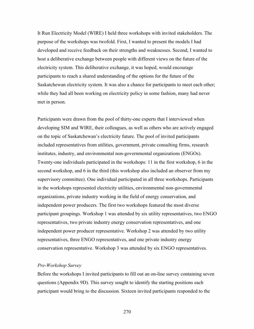
270

It Run Electricity Model (WIRE) I held three workshops with invited stakeholders. The

purpose of the workshops was twofold. First, I wanted to present the models I had

developed and receive feedback on their strengths and weaknesses. Second, I wanted to

host a deliberative exchange between people with different views on the future of the

electricity system. This deliberative exchange, it was hoped, would encourage

participants to reach a shared understanding of the options for the future of the

Saskatchewan electricity system. It was also a chance for participants to meet each other;

while they had all been working on electricity policy in some fashion, many had never

met in person.

Participants were drawn from the pool of thirty-one experts that I interviewed when

developing SIM and WIRE, their colleagues, as well as others who are actively engaged

on the topic of Saskatchewan’s electricity future. The pool of invited participants

included representatives from utilities, government, private consulting firms, research

institutes, industry, and environmental non-governmental organizations (ENGOs).

Twenty-one individuals participated in the workshops: 11 in the first workshop, 6 in the

second workshop, and 6 in the third (this workshop also included an observer from my

supervisory committee). One individual participated in all three workshops. Participants

in the workshops represented electricity utilities, environmental non-governmental

organizations, private industry working in the field of energy conservation, and

independent power producers. The first two workshops featured the most diverse

participant groupings. Workshop 1 was attended by six utility representatives, two ENGO

representatives, two private industry energy conservation representatives, and one

independent power producer representative. Workshop 2 was attended by two utility

representatives, three ENGO representatives, and one private industry energy

conservation representative. Workshop 3 was attended by six ENGO representatives.

Pre-Workshop Survey

Before the workshops I invited participants to fill out an on-line survey containing seven

questions (Appendix 9D). This survey sought to identify the starting positions each

participant would bring to the discussion. Sixteen invited participants responded to the

271

survey. This included one respondent who did not end up attending the workshops, one

respondent who did not provide a name, and fourteen participants who took part in the

workshops. Participants in the third workshop did not fill out a pre-workshop survey.

I first asked questions to understand each participant’s position on GHG emission

reductions and the technologies that could help achieve GHG reductions:

• Thinking ahead to the future, what GHG intensity should Saskatchewan strive to

achieve in the electricity sector by 2050? (Question 1)

• Several technologies might contribute to lowering the GHG intensity of

Saskatchewan's electricity system. Seventeen of these technologies are listed

below in alphabetical order. Please rank the technologies in terms of their

importance for reducing the GHG intensity of Saskatchewan's electricity system.

(Question 2)

• Imagine a preferred electricity generation mix in the year 2050 that achieves the

electricity GHG intensity you listed in Question 1. What proportion of total

electricity generation is provided by each of the following technologies in your

preferred scenario? (Question 3)

There was a range of responses to the first question (Figure 9-1). One of the participants

who wanted GHG intensity to be 0-99 grams CO2e/kWh included the note,

It is clear from the 2013 IPCC WG3 AR5 report that the whole world needs

to decarbonize fully by 2070 - and even then there will need to be multiple

decades during which we are net carbon negative after that time - if we are to

prevent climate change from going into unpredictable, likely irreversible

territory. Decarbonisation of electricity is a relatively easy component, and a

necessary prerequisite for decarbonisation of certain other sectors. Hence a

failure to decarbonize electricity by 2050 worldwide (and that includes

Saskatchewan!) would put us in a very perilous position.

(Workshop Participant)

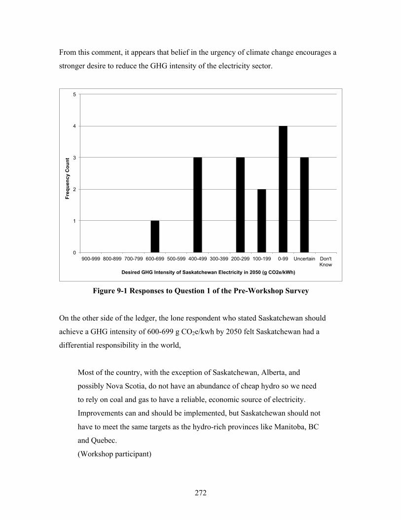
272

From this comment, it appears that belief in the urgency of climate change encourages a

stronger desire to reduce the GHG intensity of the electricity sector.

Figure 9-1 Responses to Question 1 of the Pre-Workshop Survey

On the other side of the ledger, the lone respondent who stated Saskatchewan should

achieve a GHG intensity of 600-699 g CO2e/kwh by 2050 felt Saskatchewan had a

differential responsibility in the world,

Most of the country, with the exception of Saskatchewan, Alberta, and

possibly Nova Scotia, do not have an abundance of cheap hydro so we need

to rely on coal and gas to have a reliable, economic source of electricity.

Improvements can and should be implemented, but Saskatchewan should not

have to meet the same targets as the hydro-rich provinces like Manitoba, BC

and Quebec.

(Workshop participant)

0

1

2

3

4

5

900-999 800-899 700-799 600-699 500-599 400-499 300-399 200-299 100-199 0-99 Uncertain Don't Know

Freq

uenc

y C

ount

Desired GHG Intensity of Saskatchewan Electricity in 2050 (g CO2e/kWh)

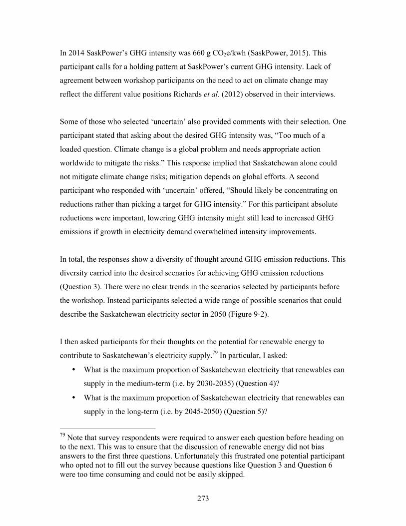
273

In 2014 SaskPower’s GHG intensity was 660 g CO2e/kwh (SaskPower, 2015). This

participant calls for a holding pattern at SaskPower’s current GHG intensity. Lack of

agreement between workshop participants on the need to act on climate change may

reflect the different value positions Richards et al. (2012) observed in their interviews.

Some of those who selected ‘uncertain’ also provided comments with their selection. One

participant stated that asking about the desired GHG intensity was, “Too much of a

loaded question. Climate change is a global problem and needs appropriate action

worldwide to mitigate the risks.” This response implied that Saskatchewan alone could

not mitigate climate change risks; mitigation depends on global efforts. A second

participant who responded with ‘uncertain’ offered, “Should likely be concentrating on

reductions rather than picking a target for GHG intensity.” For this participant absolute

reductions were important, lowering GHG intensity might still lead to increased GHG

emissions if growth in electricity demand overwhelmed intensity improvements.

In total, the responses show a diversity of thought around GHG emission reductions. This

diversity carried into the desired scenarios for achieving GHG emission reductions

(Question 3). There were no clear trends in the scenarios selected by participants before

the workshop. Instead participants selected a wide range of possible scenarios that could

describe the Saskatchewan electricity sector in 2050 (Figure 9-2).

I then asked participants for their thoughts on the potential for renewable energy to

contribute to Saskatchewan’s electricity supply.79 In particular, I asked:

• What is the maximum proportion of Saskatchewan electricity that renewables can

supply in the medium-term (i.e. by 2030-2035) (Question 4)?

• What is the maximum proportion of Saskatchewan electricity that renewables can

supply in the long-term (i.e. by 2045-2050) (Question 5)?

79 Note that survey respondents were required to answer each question before heading on to the next. This was to ensure that the discussion of renewable energy did not bias answers to the first three questions. Unfortunately this frustrated one potential participant who opted not to fill out the survey because questions like Question 3 and Question 6 were too time consuming and could not be easily skipped.

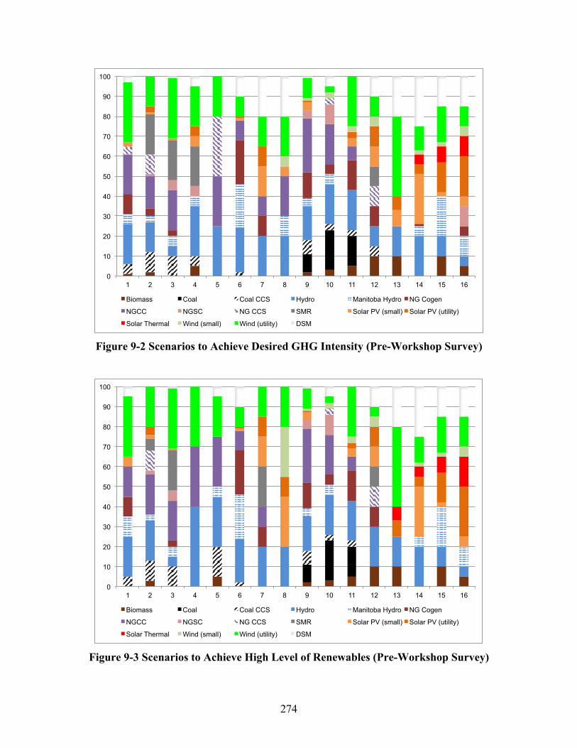
274

Figure 9-2 Scenarios to Achieve Desired GHG Intensity (Pre-Workshop Survey)

Figure 9-3 Scenarios to Achieve High Level of Renewables (Pre-Workshop Survey)

0

10

20

30

40

50

60

70

80

90

100

1 2 3 4 5 6 7 8 9 10 11 12 13 14 15 16

Biomass Coal Coal CCS Hydro Manitoba Hydro NG Cogen

NGCC NGSC NG CCS SMR Solar PV (small) Solar PV (utility)

Solar Thermal Wind (small) Wind (utility) DSM

0

10

20

30

40

50

60

70

80

90

100

1 2 3 4 5 6 7 8 9 10 11 12 13 14 15 16

Biomass Coal Coal CCS Hydro Manitoba Hydro NG Cogen

NGCC NGSC NG CCS SMR Solar PV (small) Solar PV (utility)

Solar Thermal Wind (small) Wind (utility) DSM

275

• What electricity generation mix would achieve the maximum renewable potential

you identified in Question 5 (Question 6)? (Summarized in Figure 9-3)

Questions 4 and 5 were used as markers to understand whether participants’ views would

shift through the process of deliberation at the workshop. Identical questions were asked

in the post-workshop survey (Appendix 9A). Question 6 produced a range of scenarios

that differed from those presented in response to Question 3, and were still diverse

(Figure 9-3).

The seventh and final question asked participants about barriers to expanding renewable

energy in Saskatchewan. Participants were asked to rank ten barriers in terms of whether

they were ‘Not important’, ‘Somewhat important’, or ‘Very Important’ (Table 9-1). The

list of barriers overlaps with the categories of “agreement, knowledge, technology,

economy, social, and political” used by Richards et al. (2012), but is more specific in

many instances. For example, rather than asking whether technology is a barrier I asked

specifically if the intermittency of renewable energy is a barrier. The ten barriers I asked

about in the pre-workshop survey emerged from the thirty-one interviews I conducted

during the research process (see Chapter 2).

Beliefs about cost and intermittency appear to be strongly related to the level of

renewable penetration participants felt was possible. Intermittency was particularly

polarizing, 44% of participants (7 of 16) believed it was not important, 38% of

participants (6 of 16) believed it to be very important, and only 19% (3 of 16) took the

more neutral stance that it was somewhat important.

Participants who believed cost and intermittency were ‘not important’ barriers were more

likely to believe that 100% renewable electricity generation was possible by 2050.80

These participants were also more likely to be from an ENGO background; three of the

80 Three of the four participants who believed cost was not important believed renewable electricity could meet 100% of electricity demand by 2050; three of the five who believed intermittency was not important believed 100% renewable was possible by 2050.

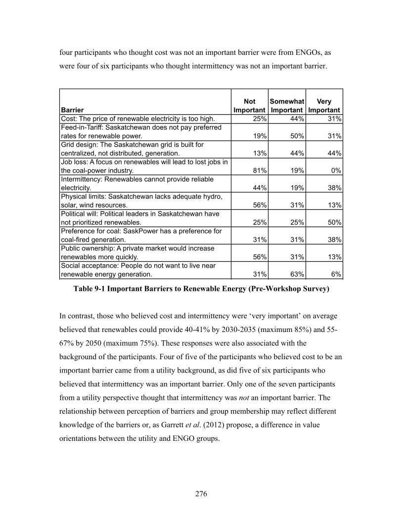
276

four participants who thought cost was not an important barrier were from ENGOs, as

were four of six participants who thought intermittency was not an important barrier.

Table 9-1 Important Barriers to Renewable Energy (Pre-Workshop Survey)

In contrast, those who believed cost and intermittency were ‘very important’ on average

believed that renewables could provide 40-41% by 2030-2035 (maximum 85%) and 55-

67% by 2050 (maximum 75%). These responses were also associated with the

background of the participants. Four of five of the participants who believed cost to be an

important barrier came from a utility background, as did five of six participants who

believed that intermittency was an important barrier. Only one of the seven participants

from a utility perspective thought that intermittency was not an important barrier. The

relationship between perception of barriers and group membership may reflect different

knowledge of the barriers or, as Garrett et al. (2012) propose, a difference in value

orientations between the utility and ENGO groups.

BarrierNot

ImportantSomewhat Important

Very Important

Cost: The price of renewable electricity is too high. 25% 44% 31%Feed-in-Tariff: Saskatchewan does not pay preferred rates for renewable power. 19% 50% 31%Grid design: The Saskatchewan grid is built for centralized, not distributed, generation. 13% 44% 44%Job loss: A focus on renewables will lead to lost jobs in the coal-power industry. 81% 19% 0%Intermittency: Renewables cannot provide reliable electricity. 44% 19% 38%Physical limits: Saskatchewan lacks adequate hydro, solar, wind resources. 56% 31% 13%Political will: Political leaders in Saskatchewan have not prioritized renewables. 25% 25% 50%Preference for coal: SaskPower has a preference for coal-fired generation. 31% 31% 38%Public ownership: A private market would increase renewables more quickly. 56% 31% 13%Social acceptance: People do not want to live near renewable energy generation. 31% 63% 6%

277

The greatest degree of consensus was found on ranking the importance of job loss. Job

loss was not seen as ‘very important’ by any of the respondents, and instead 81% (13 of

16) believed it was not important. This may be a reflection of the composition of the

participants in the deliberative workshops; affected labour groups were not represented.

The diversity of responses to the ranking of barriers showed that deliberation could be

productive. The split between representatives from utility and ENGO backgrounds

indicated a potential for conflict at the workshops.

Deliberative Modelling Workshop

The workshop was divided into six parts (see workshop script in Appendix 9B for more

detail):

1. Welcome, introductions and ground rules

2. Presentation of the history and context of the Saskatchewan electricity system

3. Model introduction and workbook exercises to examine the assumptions

4. Scenario creation

5. Opportunities and barriers discussion

6. Post-workshop survey

In the first segment I worked to generate an atmosphere of openness and respect. In

particular, participants were encouraged to “disagree without being disagreeable.”81 The

second segment was meant to provide a common basis of understanding. I presented a

condensed history of the Saskatchewan electricity system (a summary of Chapter 3), and

explained the need for investment in the electricity system to replace aging infrastructure,

meet growing demand, and comply with federal GHG legislation (a summary of Chapter

1). I also outlined the physical potential for renewable energy in Saskatchewan (a

summary of Chapter 4).

In the third segment I asked participants to break into smaller groups of 3 or 4 people.

Participants were provided with a workbook that outlined the assumptions I used in the

81 I had a facilitator helping with workshop 1, but not workshops 2 and 3. The facilitator worked to ensure that everyone had a chance to speak and be heard.

278

Saskatchewan Investment Model (Appendix 9C). In the first workshop, three sub-groups

were formed. Sub-groups were selected to maximize the institutional diversity of

representation within each group. These sub-groups were each assigned a specific part of

the workbook to review: electricity generation costs, renewable potential, or electricity

conservation cost and potential. I asked each group to discuss the assumptions I had made

and record suggestions for improvements within the workbook. The goal was to seek

agreement on the underlying assumptions before testing scenarios. After the first

workshop I received feedback that the sub-groups did not have enough time to adequately

review the workbook and felt rushed. In subsequent workshops this segment was

combined with scenario creation.

In the fourth segment sub-groups were tasked with generating scenarios that could be

analyzed using iSIM (Model 9A). In the first workshop, the sub-groups formed to

evaluate the workbooks were shuffled so that a representative from each original sub-

group (and with knowledge of the particular model area they had focused on: cost,

renewable potential, or energy conservation potential) was present in every scenario-

building group. This step was also used to increase interactions between diverse

participants. In subsequent workshops the groups did not exchange members, but instead

worked as teams to compete against the other group in their scenario achievement. Once

the sub-groups had come to an agreement on a scenario for Saskatchewan’s electricity

future, that information was placed in SIM either by a ‘modeller’; i.e. a participant

assigned to interact with the laptop in each group, or by me.82

The interactive SIM model was designed to strike a “balance between the simplicity

needed to make the model ‘fun to use’ and the complexity required to make it ‘true to

life’” (Carmichael et al., 2004: 173). It was built in Excel, since it is a commonly used

software and many participants have experience using it. It was accompanied by a

82 This worked well in the second and third workshops, which had two scenario building groups, but proved challenging in the first workshop where there were three scenario-building groups.

279

workbook (Appendix 9C) that walked participants through the various inputs they could

control in the model. Participants could design scenarios in SIM by:

1. Changing assumptions used in the model related to capital cost, O&M costs, and

cost improvement factors;

2. Changing constraints used in the model related to conservation potential, wind

integration potential, hydroelectric potential, and biomass potential;

3. Changing assumptions regarding growth of electricity demand;

4. Assigning a carbon price in each time-step;

5. Assigning a minimum proportion of electricity generated in 2050 for desired

technologies;

6. Assigning a maximum proportion for small, modular nuclear reactors, which

allowed groups to turn the nuclear option on or off.

The customized scenario was then optimized using Frontline Solver in Excel. The

objective function in the interactive model is the same as that found in SIM (see

Appendix 7A). The optimization finds the least-cost path to supplying Saskatchewan’s

electricity, while meeting the constraints specified by the group, and using the cost,

renewable potential, conservation potential, and demand growth assumptions assumed by

the group. Figure 9-4 presents a screen-shot from the scenario design interface of iSIM.

Figure 9-4 Scenario Building Screen in SIM

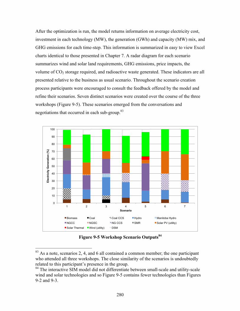
280

After the optimization is run, the model returns information on average electricity cost,

investment in each technology (MW), the generation (GWh) and capacity (MW) mix, and

GHG emissions for each time-step. This information is summarized in easy to view Excel

charts identical to those presented in Chapter 7. A radar diagram for each scenario

summarizes wind and solar land requirements, GHG emissions, price impacts, the

volume of CO2 storage required, and radioactive waste generated. These indicators are all

presented relative to the business as usual scenario. Throughout the scenario creation

process participants were encouraged to consult the feedback offered by the model and

refine their scenarios. Seven distinct scenarios were created over the course of the three

workshops (Figure 9-5). These scenarios emerged from the conversations and

negotiations that occurred in each sub-group.83

Figure 9-5 Workshop Scenario Outputs84

83 As a note, scenarios 2, 4, and 6 all contained a common member; the one participant who attended all three workshops. The close similarity of the scenarios is undoubtedly related to this participant’s presence in the group. 84 The interactive SIM model did not differentiate between small-scale and utility-scale wind and solar technologies and so Figure 9-5 contains fewer technologies than Figures 9-2 and 9-3.

0

10

20

30

40

50

60

70

80

90

100

1 2 3 4 5 6 7

Ele

ctri

city

Gen

erat

ion

(%)

Scenario

Biomass Coal Coal CCS Hydro Manitoba Hydro

NGCC NGSC NG CCS SMR Solar PV (utility)

Solar Thermal Wind (utility) DSM

281

I travelled around the room helping the sub-groups as they created their scenarios. In the

first workshop I heard feedback that participants would like improvements to the user

interface. I improved the interface for the subsequent workshops. In the second

workshop, one participant expressed dismay that the model had added in natural gas

combined cycle with CCS “against our wishes” (scenario 4 in Figure 9-5). The

participant did not like this technology and disagreed that it should be included. This was

an opportunity to discuss the model assumption that dispatchable capacity must meet

peak demand; natural gas with CCS has been added to ensure peak demand could be met.

This discussion led the participant to revisit the model and redesign the scenario. It

appeared to me to be a good example of learning through the discipline imposed by the

model.

At the end of the scenario creation exercise the sub-groups were brought together at a

plenary roundtable to discuss the scenarios they had generated. Each sub-group was

asked to present their scenario. A reporter from each sub-group discussed the electricity

generation mix they had generated and explained their group’s choices. I was sure to note

the final price and GHG emission implications of each scenario to encourage a

competitive spirit between the teams.

The final interactive component of the workshop was a brainstorming exercise to identify

barriers to renewable energy in Saskatchewan and opportunities for overcoming these

barriers. Participants were each given a pad of sticky notes and asked to write down as

many barriers as they could think of in five minutes. Myself, with help from the

facilitator in workshop 1 and a member of my supervisory committee in workshop 2,

walked around the room grabbing the sticky notes when they were completed and posting

them on a wall. We organized the barriers into related clusters as we posted them on the

wall. Following this, participants were asked to volunteer explanations for the barriers

they had posted. This provided a chance for clarification and discussion. We then

repeated the exercise with different coloured sticky notes and asked participants to

brainstorm opportunities for overcoming the barriers. Means of overcoming barriers were

posted alongside related barriers. Another round of discussion followed before the

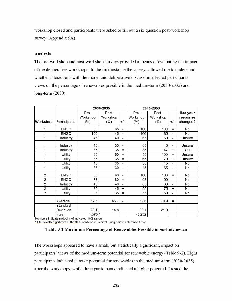
282

workshop closed and participants were asked to fill out a six question post-workshop

survey (Appendix 9A).

Analysis

The pre-workshop and post-workshop surveys provided a means of evaluating the impact

of the deliberative workshops. In the first instance the surveys allowed me to understand

whether interactions with the model and deliberative discussion affected participants’

views on the percentage of renewables possible in the medium-term (2030-2035) and

long-term (2050).

Table 9-2 Maximum Percentage of Renewables Possible in Saskatchewan

The workshops appeared to have a small, but statistically significant, impact on

participants’ views of the medium-term potential for renewable energy (Table 9-2). Eight

participants indicated a lower potential for renewables in the medium-term (2030-2035)

after the workshops, while three participants indicated a higher potential. I tested the

Pre-Workshop

(%)

Post-Workshop

(%) +/-

Pre-Workshop

(%)

Post-Workshop

(%) +/-

1 ENGO 85 65 - 100 100 = No1 ENGO 100 45 - 100 85 - No1 Industry 45 40 - 65 60 - Unsure

1 Industry 45 35 - 85 45 - Unsure1 Industry 35 35 = 35 47 + Yes1 Utility 35 60 + 55 100 + Unsure1 Utility 35 35 = 65 70 + Unsure1 Utility 45 35 - 55 45 - No1 Utility 35 30 - 45 65 + No

2 ENGO 85 60 - 100 100 = No2 ENGO 75 80 + 95 90 - No2 Industry 45 40 - 65 60 - No2 Utility 35 45 + 55 75 + No2 Utility 35 35 = 55 50 - No

Average 52.5 45.7 - 69.6 70.9 =Standard Deviation 23.1 14.8 22.1 21.0t-test 1.375 * -0.232

Numbers indicate midpoint of indicated 10% range* Statistically significant at the 90% confidence interval using paired difference t-test

2030-2035 2045-2050Has your response changed?ParticipantWorkshop

283

difference between the pre-workshop and post-workshop responses using a t-test and

found a statistically significant decrease in participants’ views on medium-term

renewable potential at the 90% confidence interval. Using this same approach I find that

the workshops did not have a statistically significant impact on participants’ views of

renewable potential in the long-run (2045-2050). This lack of movement on participants’

responses was echoed by their answers to the question: “Has your response changed from

the earlier survey?” Nine participants stated their response did not change; any difference

may have been an error of memory, rather than a change in perspective. Only one person

stated their response did change as a result of the workshops. This person explained that

they, “Learned more about actual potential and costs of various resources through

interaction with informed participants.”

The pre- and post-workshop surveys also allowed me to understand whether perspectives

had shifted on the barriers to renewable energy expansion in Saskatchewan. The

discussion of barriers in the workshops uncovered themes very similar to those outlined

by Richards et al. (2012) (see Table 9-3). The barrier mentioned most often (35

responses) was the lack of political and policy support for renewables. This lack of

support was expressed with notes such as:

• Lack of federal emissions targets;

• Lack of government leadership;

• Lack of political will to address climate crisis;

• Lack of support mechanisms such as Feed-in-Tariff (FIT);

• Lack of carbon pricing.

To overcome this barrier participants recommended implementing many of the policies

currently lacking such as GHG emission reduction targets, carbon pricing, and feed-in-

tariffs.

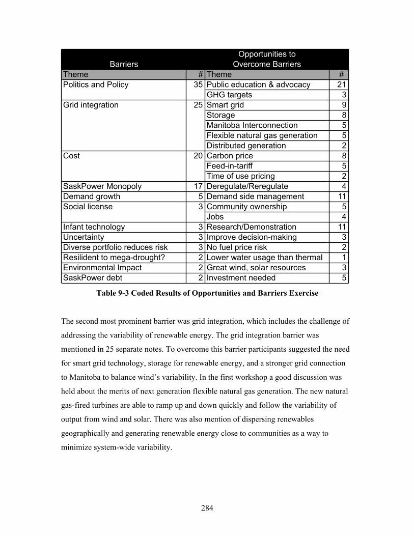
284

Table 9-3 Coded Results of Opportunities and Barriers Exercise

The second most prominent barrier was grid integration, which includes the challenge of

addressing the variability of renewable energy. The grid integration barrier was

mentioned in 25 separate notes. To overcome this barrier participants suggested the need

for smart grid technology, storage for renewable energy, and a stronger grid connection

to Manitoba to balance wind’s variability. In the first workshop a good discussion was

held about the merits of next generation flexible natural gas generation. The new natural

gas-fired turbines are able to ramp up and down quickly and follow the variability of

output from wind and solar. There was also mention of dispersing renewables

geographically and generating renewable energy close to communities as a way to

minimize system-wide variability.

BarriersOpportunities to

Overcome BarriersTheme # Theme #Politics and Policy 35 Public education & advocacy 21

GHG targets 3Grid integration 25 Smart grid 9

Storage 8Manitoba Interconnection 5Flexible natural gas generation 5Distributed generation 2

Cost 20 Carbon price 8Feed-in-tariff 5Time of use pricing 2

SaskPower Monopoly 17 Deregulate/Reregulate 4Demand growth 5 Demand side management 11Social license 3 Community ownership 5

Jobs 4Infant technology 3 Research/Demonstration 11Uncertainty 3 Improve decision-making 3Diverse portfolio reduces risk 3 No fuel price risk 2Resilident to mega-drought? 2 Lower water usage than thermal 1Environmental Impact 2 Great wind, solar resources 3SaskPower debt 2 Investment needed 5

285

The importance of the grid integration barrier aligns with Richards et al. (2012) who

found that technology was the most frequently mentioned barrier. Richards et al. (2012)

also heard participants offer many of the same solutions, such as smart grids, storage and

geographic dispersion.

The cost of renewable technology was mentioned as a barrier on twenty separate sticky

notes. To overcome this barrier, real or perceived, participants suggested changing the

pricing system. Carbon pricing would level the playing field with fossil-fuel

technologies, as would an end to fossil-fuel subsidies. A feed-in-tariff would provide a

better price to private power producers. Full-cost accounting would ensure that

externalities besides GHG emissions were considered. The study by Richards et al.

(2012) also found that cost was a perceived barrier.

Other barriers that appeared were complaints about SaskPower’s monopoly control of the

Saskatchewan grid. This control led some to call for deregulation and a competitive

market, while others disagreed and suggested re-regulation would be better. Re-

regulation would keep the power system in public control, while also opening up the

possibility of community generation of renewable energy. Other barriers mentioned on

only a few occasions, were social license, the challenge of making decisions under

uncertainty, and the environmental impacts of renewables (one note read “concern about

wildlife impact, real or not”). Frequently mentioned means of overcoming barriers were

further renewable energy research projects and renewable energy demonstration projects

in Saskatchewan.

The promise of a deliberative exchange is that understanding can be gained and positions

can shift. To understand whether participants had shifted their thinking about the barriers

that face renewable energy in Saskatchewan, the post-workshop survey included a final

question asking people to indicate which barriers were “very important”. It was possible

to compare the answers to the pre-workshop survey and post-workshop survey for

fourteen participants (Table 9-4). The results show that the four-hour workshop did not

lead to substantial shifts in thinking about barriers. In only two instances did a participant

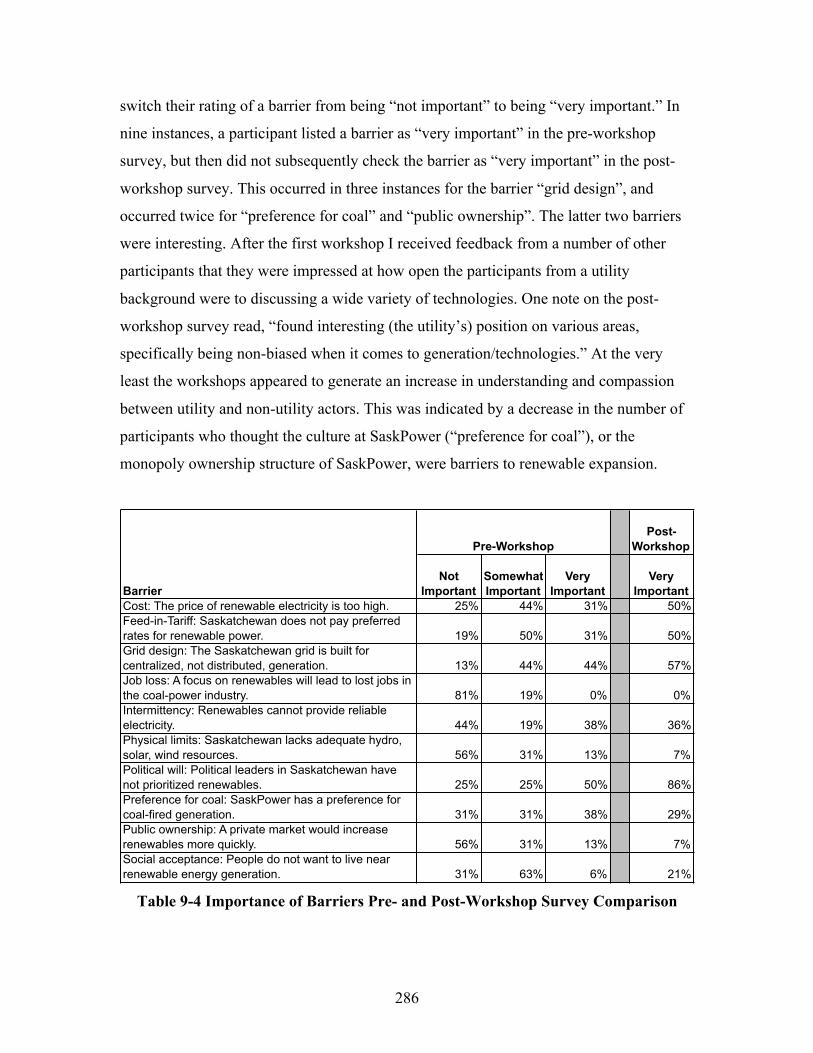
286

switch their rating of a barrier from being “not important” to being “very important.” In

nine instances, a participant listed a barrier as “very important” in the pre-workshop

survey, but then did not subsequently check the barrier as “very important” in the post-

workshop survey. This occurred in three instances for the barrier “grid design”, and

occurred twice for “preference for coal” and “public ownership”. The latter two barriers

were interesting. After the first workshop I received feedback from a number of other

participants that they were impressed at how open the participants from a utility

background were to discussing a wide variety of technologies. One note on the post-

workshop survey read, “found interesting (the utility’s) position on various areas,

specifically being non-biased when it comes to generation/technologies.” At the very

least the workshops appeared to generate an increase in understanding and compassion

between utility and non-utility actors. This was indicated by a decrease in the number of

participants who thought the culture at SaskPower (“preference for coal”), or the

monopoly ownership structure of SaskPower, were barriers to renewable expansion.

Table 9-4 Importance of Barriers Pre- and Post-Workshop Survey Comparison

Post-Workshop

Not Important

Somewhat Important

Very Important

Very Important

Cost: The price of renewable electricity is too high. 25% 44% 31% 50%Feed-in-Tariff: Saskatchewan does not pay preferred rates for renewable power. 19% 50% 31% 50%Grid design: The Saskatchewan grid is built for centralized, not distributed, generation. 13% 44% 44% 57%Job loss: A focus on renewables will lead to lost jobs in the coal-power industry. 81% 19% 0% 0%Intermittency: Renewables cannot provide reliable electricity. 44% 19% 38% 36%Physical limits: Saskatchewan lacks adequate hydro, solar, wind resources. 56% 31% 13% 7%Political will: Political leaders in Saskatchewan have not prioritized renewables. 25% 25% 50% 86%Preference for coal: SaskPower has a preference for coal-fired generation. 31% 31% 38% 29%Public ownership: A private market would increase renewables more quickly. 56% 31% 13% 7%Social acceptance: People do not want to live near renewable energy generation. 31% 63% 6% 21%

Pre-Workshop

Barrier

287

There was little shift in ranking of the barrier “intermittency”. Of the fourteen

respondents for which I had both pre- and post-workshop surveys, five had indicated

intermittency was very important before the workshop and four continued to indicate that

intermittency was very important after the workshop. One participant changed their

ranking of intermittency from “somewhat important” to “very important.” This highlights

the problem that may have been created by switching the format of the question from a

three-option scale in the pre-workshop survey to a simple checkmark to indicate “very

important” in the post-workshop survey. The post-workshop survey was, however,

designed to be quick and easy to answer so that participants would be willing to fill it out

before leaving the workshop.

The one area where thinking did seem to converge was in regards to the barrier “political

will”. In the pre-workshop survey 50% (8 participants) thought a lack of political will

was a “very important” barrier, 25% (4 participants) thought it was “somewhat

important”, and 25% (4 participants) thought it was “not important”. Following the

workshops, 86% of participants (12 of 14) thought lack of political will to be a “very

important” barrier. Three participants had upgraded the barrier from being “somewhat

important” to being “very important” and one participant upgraded the barrier from being

“not important” to “very important.” This is particularly telling when compared with the

results in Table 9-3. Political leaders have failed to introduce the policies that would see

renewables thrive. With political will it would be possible to change the relative costs of

renewables, give increased impetus to GHG emission reductions, fund research and

education on climate change and renewable energy, negotiate co-operative agreements

with Manitoba Hydro, and provide SaskPower with a clarity of purpose. Lacking political

will, renewables will continue to face barriers to expansion.

Conclusions

The deliberative modelling workshops were an attempt to nurture a shared understanding

between Saskatchewan’s electric utilities and ENGOs calling for more renewables. Over

the course of four hours, participants were asked to work together to imagine scenarios

for Saskatchewan’s electricity future. The exercise succeeded, to a certain extent, at

288

creating sentiments of compassion and mutual respect. All of the workshop participants

responded yes to the questions, “Have you learned anything from this workshop?” and

“Did you enjoy the experience of interacting with others at the workshop?” Post-

workshop surveys included comments like “useful discussion” and “very stimulating –

always fun to talk to folks with different priorities and backgrounds.” The participants

appeared genuinely curious to learn about each other’s perspectives.

The four-hour workshop did not appear to substantially shift the perspectives of

participants. The only noticeable change was a slight decrease in the level of renewable

energy participants felt was possible in the medium-term (2030-2035; Table 9-2). This

may mean that the workshop created a better understanding of the constraints that

currently affect the electricity system, which caused participants to revise renewable

potential downwards. Participants generally did not shift their perspectives on the barriers

to renewable energy expansion. They did, however, achieve a near consensus that ‘lack

of political will’ is a barrier to encouraging renewables in the province.

Shortcomings

The deliberative modelling workshops I hosted required a specialist level of knowledge

of the electricity sector. I realized that it would be difficult to find a group of participants

that were knowledgeable enough of the specifics of the electricity industry to offer useful

advice on the modelling assumptions and who were also representative of the

Saskatchewan population. Participants at the workshops were skewed to representatives

from utilities, private consulting companies in the electricity conservation sector, and

ENGOs. This highlights the “representation problem” of deliberative exercises (Zografos

and Howarth, 2010). The workshop participants were not representative of Saskatchewan

society at large. Participants were predominantly from European-settler backgrounds and

all but two were men. This reflected the pool of potential participants I had invited; only

four of the thirty-one stakeholders I interviewed were female. The Saskatchewan utility

sector and ENGO sector appear to be predominantly male; at least at the management-

level or board-level.

289

To host a deliberative conversation with members of the broader, non-specialist,

Saskatchewan public, I would need to make modifications to the workshop format. Less

time would be spent investigating assumptions, and more time could be spent presenting

a range of pre-set scenarios and indicators. The conversation could then focus on the

trade-offs faced when choosing between electricity scenarios.

van den Belt’s (2002) Mediated Modeling approach offers a deeper level of participant

engagement than the deliberative modelling process I carried out. In the mediated

modelling process participants sign on to participate over the course of months or years.

Participants meet regularly, providing input on the research questions, the structure of the

model, and contributing research effort to developing and improving the model. The

advantage of the much less elaborate deliberative modelling approach I used was that

participation was easy; only a brief pre-workshop survey was completed beforehand, the

workshop was scheduled for one four-hour afternoon session, and participants were not

assigned any homework when they left.

The light level of participation in the deliberative workshops was not enough to generate

significant movement towards consensus. If financial resources allowed, it would be

interesting to trial a more intensive mediated modelling process to see if a greater degree

of consensus could be achieved.

There would likely be substantial barriers that could prevent stakeholders from

participating in a mediated modelling process. I found that, even with the relatively light

commitment required, there were barriers to participation in the deliberative workshops.

One invited participant could not participate because his organization did not have the

budget to spare his time during work hours. Another invited participant chose not to

participate because he felt he could be more candid in an interview setting than in a

setting with professionals from the electricity field, especially representatives from the

SaskPower utility. The comment from this would-be participant highlighted that “power

relations are not simply left at the door of deliberative forums” (Howarth, 2010: p. 3409).

Power – political and social – is present in a deliberative modelling exercise.

290

In Saskatchewan, as in many regulated electricity markets, SaskPower has a monopoly on

the supply of electricity. This market power is enshrined in the Saskatchewan Power

Corporations Act. Self-generation of renewables is a threat to the market power that

SaskPower fought to gain, from its incorporation in 1949 to the purchase of the Regina

power plant in 1965. This may explain the different perception of barriers between

ENGO and industry representatives. To a renewable energy advocate a feed-in-tariff is a

way to encourage renewables in the province. To SaskPower a feed-in-tariff is a cost; it

requires the corporation to pay market rates (or above) for electricity generated by

producers who are meanwhile eroding SaskPower’s market share, and thereby creating

“stranded assets” out of existing generation and transmission equipment. The issue of

integrating variable renewables is similar. For renewable advocates, the solutions to

intermittency are readily available. But, as Sovacool (2009) observes, “Technically, these

technologies can be incorporated into the grid easily. Socially, much institutional

resistance remains” (p. 4506). Utilities find more comfort in “conservative inventions”

like coal-fired generation with carbon capture and storage (CCS) or small, modular

nuclear reactors because these centralized technologies maintain monopolistic market

power (Sovacool, 2009). This preference was certainly expressed in the pre-workshop

survey where respondents from SaskPower typically ranked coal with CCS as the 3rd

most important technology for achieving a desired 2050 GHG intensity (mode ranking,

median was 3.5) and ranked small, modular nuclear reactors 6th most important (mode

and median both 6). The other respondents most often ranked coal with CCS or small,

modular nuclear reactors dead last (the median ranking of coal with CCS amongst non-

SaskPower participants was 12th and the mode was 17th, while the median ranking of

small, modular nuclear reactors was 13th and the mode was again 17th). There is a very

clear split in support for these “conservative inventions.” Concerns over intermittency

may be less a technical barrier, and more a result of institutional resistance. An open-

ended discussion in a deliberative modeling workshop may not be the best way to discuss

these issues, as it involves questioning the motivations of some of the participants. It may

be hard to “disagree without being disagreeable” when entering into such a discussion.

291

Chapter 10 – Conclusions and Next Steps

Findings

In this dissertation I set out to ask, what is the cost of Greening the Saskatchewan Grid

by lowering greenhouse gas (GHG) emissions by 80% or more by 2050 with a renewable

energy focused electricity pathway? To understand the relative cost of a renewable

energy pathway I needed to know the costs of alternative scenarios, including a business-

as-usual scenario (SaskPower BAU), and scenarios for lowering GHG emissions that

featured technologies like carbon capture and storage (CCS) and small modular nuclear

reactors. I built the Saskatchewan Investment Model (SIM) to understand the costs of

these various scenarios.

Building SIM required me to answer a number of intermediate questions. I needed to

know how electricity demand might change between 2015 and 2050. I created an

electricity demand forecast in Chapter 6 to answer that question. I needed to know how

much potential there is in Saskatchewan to generate renewable electricity from wind,

water, sun, and biomass. I outlined Saskatchewan’s renewable potential in Chapter 4. I

needed to know the relative costs and operating characteristics of competing electricity

generation technologies, including their capital costs, operating costs, capacity factors,

expected life, and fuel efficiency. Those costs and characteristics are examined in

Chapter 5. I also needed to know how these costs and characteristics would change over

time; SIM includes exogenous cost improvement factors that forecast changes in capital

and operating costs due to technological progress. I also created fuel price forecasts to

understand how the price of coal, natural gas, biomass and uranium might change over

time. Both the cost improvement factors and future fuel prices are uncertain and so I

conducted a sensitivity analysis to account for the uncertainty of these estimates (Chapter

7).

After conducting this analysis I found that a Greening the Grid leadership scenario would

cost about two cents per kilowatt-hour (kWh) more than a business-as-usual scenario by

2050. The Greening the Grid scenario would, however, cut cumulative GHG emissions

292

in half, reduce water use, and create more jobs (Chapter 8). It would also reduce

emissions without adding significantly to the volume of stored CO2 and would not result

in the creation of any long-lived radioactive waste (Chapter 8). The Greening the Grid

scenario would also be resilient to carbon pricing. If Canada or Saskatchewan were to

implement an escalating carbon pricing policy, that begins at $15/tonne in 2015 and

increases by $15 every 5-year time-step, the total discounted cost of the Greening the

Grid scenario would be comparable to the other scenarios.

Because of my focus on a renewable energy pathway I paid particular attention to the

issue of variability. Renewable energy sources like wind, water, and solar are naturally

variable in their electricity output. From the Premier of Saskatchewan to SaskPower

management there is a concern that the variability of renewable energy will create a

shortage when it is needed most. In this dissertation I asked, what is the cost of building

adequate storage capacity and back-up capacity to ensure a renewable focused scenario

can provide a reliable supply of electricity?

To answer this question I allowed electricity storage to be built in tandem with wind and

solar facilities in SIM. I then created an hourly operations model, the WIRE model

(Appendix 7B). I used the WIRE model to test whether each of the scenarios outlined in

Chapter 7 could meet forecast hourly electricity demand in 2050 while responding to

variations in renewable energy output and electricity demand.

This step led to an iterative process of creating an investment scenario in SIM and then

checking to see ‘Will-it-Run?’ in the WIRE model. I found that, in order to provide

reliable electricity, a renewable energy focused scenario must be resilient to the seasonal

availability of solar power and hydroelectricity. Applying a ‘Liebig’s Law of the

Minimum’ for electricity planning, I revisited assumptions in the SIM model and created

the Greening the Grid scenario based on the minimum capacity factor for solar (11% in

December) and the minimum average capacity factor for hydroelectricity (43% in

March). By planning for the times when renewable electricity generation technologies are

at their seasonal low points, I found that a renewable focused Greening the Grid scenario

293

could reliably meet hourly electricity demand even in the depths of winter when

electricity demand peaks.

Key to managing the variability of renewable energy are technologies like electricity

storage, demand side management (DSM) peak shifting, and hydroelectric facilities that

can store water in reservoirs. Electricity storage and hydroelectric facilities with

reservoirs provide dispatchable power that balances the variability of the wind. DSM

peak shifting helps to smooth out net electricity demand, reducing the peaks and

increasing the troughs.85

This finding is not in itself enough to prove the technical viability of the Greening the

Grid scenario. A model is after all a simplification of a real-world system. I have

abstracted from the workings of the Saskatchewan electricity system in several ways.

First, my analysis was not spatial; I did not map the location of proposed electricity

facilities for each scenario, nor did I explicitly model the transmission and distribution

system. More engineering analysis could be done to design, model and test a Greening

the Grid scenario for Saskatchewan.

What I did succeed in modelling were the likely costs of lowering GHG emissions in the

Saskatchewan electricity sector using renewable energy. I found that planning for a

renewable energy system using a modified ‘Liebig’s Law of the Minimum’ results in an

overbuilt system and this increases costs. In the summer, when solar power and

hydroelectricity are abundant, electricity production from wind and solar exceeds total

electricity demand and has to be curtailed. Seasonal energy storage using a technology

like electrolytic hydrogen could provide a means of using that curtailed energy. This

would allow an electricity system planner to reduce the size of the Greening the Grid

system. Whether this would save money would depend on whether the value of curtailed

electricity is high enough to pay for the hydrogen conversion facilities. My research

could be extended by pursuing that line of inquiry.

85 Net electricity demand equals electricity demand minus variable renewable electricity output.

294

Barriers to Renewable Energy Expansion

In general, the results of the WIRE modelling indicated that renewable energy variability

does not appear to be a technical barrier to a Greening the Grid scenario. Technologies

exist that can balance the variability of wind and solar, at a cost. The premium paid for

balancing renewable energy variability using electricity storage, hydroelectricity, and an

overbuilt system increases the cost of electricity, but not drastically.

If renewable energy variability and cost are not barriers to the pursuit of a Greening the

Grid scenario, then what barriers might exist? I worked to explore barriers to and

opportunities for renewable expansion in three deliberative modelling workshops. As

expected, several workshop participants felt that cost and “intermittency” were

significant barriers to higher penetrations of renewable electricity in Saskatchewan.

These positions did not appear to shift over the course of a four-hour workshop and were

largely associated with utility-affiliated participants. But stakeholders from a variety of

backgrounds also came to a near consensus that renewable energy expansion is held back

by political barriers.

Nationally, Canada lacks a carbon price or hard GHG emission reduction targets. The

federal government did introduce a coal-fired electricity regulation and SaskPower plans

to meet (but not exceed) the requirements of the regulation by outfitting select coal plants

with carbon capture and storage. That regulation will reduce Saskatchewan’s electricity

sector GHG emissions by approximately half, but the gains will be temporary. I project

that GHG emissions in the SaskPower BAU scenario will begin to increase by 2045 as

natural-gas fired plants expand to meet growing electricity demand.

Provincially, Saskatchewan also lacks a carbon price and a GHG emission reduction

target. The Saskatchewan Party government also lacks motivation to get serious on the

climate change file. Premier Brad Wall told media in October 2015 that he would attend

the 2015 Paris climate change summit “to make sure that whatever Canada is committing

to doesn’t kneecap our economy in the west” (CBC, 2015). Aside from the Boundary

295

Dam III carbon capture and storage project Premier Wall has not taken any significant

action to reduce GHG emissions in the province.

Within SaskPower there is path dependence and a coal culture that has made coal with

carbon capture and storage (CCS) the preferred GHG emission reduction solution; at least

until small modular nuclear reactors prove out. Both coal with CCS and nuclear reactors

support SaskPower’s centralized control of the grid. They are “conservative”

technologies in that they maintain the existing institutional arrangements and institutional

power of SaskPower (Sovacool, 2009).

SaskPower is living through a critical time, however, when their credibility has been

damaged. CEO Robert Watson was forced to resign in 2014 after smart meters installed

in the province began to spontaneously start on fire. The heat was on SaskPower again in

Fall 2015 when it was revealed that the Boundary Dam III CCS plant was not operating

at full capacity, and was instead paying millions of dollars in penalties to Cenovus for

failing to deliver CO2 (Leo, 2015).

As the costs mount for the Boundary Dam III project, and criticism builds, SaskPower

may wish to recall Ross Thatcher’s test for public ownership. A crown would be held in

public ownership if it provided “an essential service which private firms are unable to

supply at a comparable cost to the public”, offered “a particularly satisfactory return on

invested public funds”, or provided “useful employment which otherwise would not be

available” (Thatcher quoted in Rediger, 2004: 76). The first criterion is currently in

question. SaskPower has used its monopoly position to subsidize the Boundary Dam III

CCS project, increasing the cost of electricity generation relative to other pathways for

meeting the federal coal-fired GHG regulation. On the second criterion, the crown

corporation has been raising rates, but its financial situation is so tenuous that it will not

offer dividends to the Saskatchewan government anytime in the foreseeable future. The

third criterion, providing “useful employment” appears to be the saving grace as the

government works to save jobs in the coalmines. A hard look at employment in

competing pathways, especially renewable pathways, could change that perspective. I

296

found that renewable-focused scenarios offered more job opportunities than the

SaskPower BAU pathway focused on preserving coal jobs.

There were people I interviewed who argued that deregulation would be the best path

forward for the Saskatchewan electricity system. Opening the grid up to private power

producers would continue the work begun by CEO Jack Messer in the early 1990s.

Advocated of de-regulation believed that it would spur the wide-scale adoption of low-

cost wind power. Others argued that re-regulation was needed. They argued the

Saskatchewan Power Corporation Act should be amended to allow independent

electricity producers into the market, but that electricity generation was best carried out

by municipalities, community co-operatives, and residential and commercial customers.

SaskPower’s role in this context would be as keeper of the electricity commons; the

shared transmission and distribution network that has been built up over the past eighty-

five years. In Chapter 8 I outlined the possibility of grid defection and the utility death

spiral. Death in this instance could refer to death of SaskPower’s current business model.

The question remains, will SaskPower continue to resist private power generation and the

grid defection it might encourage? Or will SaskPower embrace a new business model?

People Power

From my analysis of the Saskatchewan electricity system I find support for Sovacool’s

(2009) assertion that an electricity system is more than a collection of electricity

generators connected by wires. Instead, it is “a set of social, cultural, economic, and

political interests fused together with technology” (Sovacool, 2009: 4502). The coal-

hydro nexus that defined the past sixty years of electricity generation in Saskatchewan

has created a political constituency of coalminers, SaskPower employees, and politicians

committed to keeping coal alive. A focus on centralized power generation has made

nuclear energy a popular substitute if coal is to be abandoned. It is difficult to tell where

technological and economic analysis ends and cultural and political interests begin.

Schumpeter (1942) argued that capitalism is driven by creative destruction. Renewable

electricity technologies like wind and solar, as well as storage technologies like lithium-

297

ion batteries, have disruptive potential. They do not fit into the existing socio-technical

structure of the Saskatchewan electricity system. They do, however, fit well in the low-

density, dispersed Saskatchewan electricity grid.

Creative destruction is not pretty. There are winners and losers. Without continued

enthusiasm for CCS, the coalminers fear they will lose their jobs. However, with strategic

investment in wind, solar, and electricity storage, especially in southeast Saskatchewan,

these power workers can transition from mining the Earth to harnessing the power of the

wind and sun.

Without questioning their commitment to large-scale, costly ventures like coal with CCS

and nuclear power, SaskPower is likely to lose. The utility death spiral beckons utilities

that do not realize the potential for increasing electricity prices and increasingly

affordable renewable technologies to encourage grid defection.

The winners will be those who see the opportunities presented by greenhouse gas

emissions reductions and disruptive renewable technologies, and who are able to inspire

public support for their ideas. Saskatchewan citizens are intelligent, hard-working,

progressive people. They have been leaders in agricultural innovation. They have been

leaders in social policy innovation (e.g. socialized medicine). They have been leaders in

energy conservation (the German sounding Passivhaus concept was inspired by the

Saskatchewan Conservation House; Huck, 2015). That leadership is present in projects

like the Cowessess wind and storage facility located east of Regina, which is

demonstrating that we have overcome the technical barriers to renewable energy

expansion. Applied to the electricity system, there is no telling what that leadership could

achieve; five hundred landowners could change the course of history if they committed to

installing wind and solar facilities on their lands.

Saskatchewan people also take pride in being neighbourly, offering a hand when it is

needed. Climate change demands that we pitch in and lend a hand. It demands that we

contribute our fair share to efforts to stop catastrophic climate change. If the

298

consequences of climate change were broadly understood (and the voices of climate

change denial rightly quieted), I believe the people of Saskatchewan would rally for

change.

And change can happen quickly. The T.C. Douglas government brought electricity to

rural Saskatchewan within a four-year term. The achievement took political will and it

took the will of the people to get involved. Rural families worked to erect power poles

and string lines to bring electricity to their farms. There is a window opening to Green

the Saskatchewan Grid. Will the citizens of Saskatchewan seize the opportunity?

Least-cost economic analysis is likely not enough to inspire citizens to Green the

Saskatchewan Grid. A quote from David Orr summarizes the failings of this approach,

“A great deal has been said about the potential for least-cost, end-use

analysis that hitches narrow economic rationality to the efficient use of

resources with better technology. This is all to the good. However,

problems arise when the same economic rationality causes consumers to

observe that least cost is not the same as full cost. For example, the fully

informed consumer, armed with least-cost reasoning, would certainly

choose to buy compact fluorescent lightbulbs that have lower lifetime

costs than incandescent bulbs. But the same narrow economic rationality

would cause that consumer to refuse to pay higher utility costs to clean up

nuclear wastes and decommission reactors used to generate the electricity

that is used with greater efficiency. At this point, economic rationality

stops and virtue begins. Least-cost reasoning applies to those costs that

must be paid now; full cost applies to those costs that can be pushed onto

others or deferred to our children. Only people who take their obligations

seriously, people of virtue, would willingly pay the full costs of their

actions or even demand to do so.”

(Orr, 1994: 63)

299

The UDP process of 2009 presented citizens with a vision of a nuclear-powered

electricity future. Citizens asked, why was renewable energy not considered? Critics

responded that the variability of renewable energy and cost were significant barriers. This

dissertation has shown that a renewable energy pathway is not only possible, it is

affordable, and it creates jobs. The barriers to Greening the Saskatchewan Grid are

political, not technical or economic.

Democracy begins where least cost economic analysis ends. The scenarios I have

outlined in this dissertation produce a range of impacts: economic, ecological and social.

Choosing which electricity pathway to embrace is a political and moral decision, not an

economic decision.

The real work begins now that the dissertation is complete; the work of building

understanding of climate change; the work of deliberating pathways for a Green

electricity future; and the work of calling on the citizens of Saskatchewan to act with

virtue and determination to make a better world. As Tommy Douglas once said, it is not

too late to build one.

300

References

Aboriginal Affairs (2011) Aboriginal Consultation and Accommodation - Updated

Guidelines for Federal Officials to Fulfill the Duty to Consult. Ottawa, ON: Government

of Canada. Available on-line at: http://www.aadnc-

aandc.gc.ca/eng/1100100014664/1100100014675. Last accessed October 20, 2015.

Acres, H.G. and Company (1931) Report on the Proposed LaCorne Hydro-electric

System. Niagara Falls, ON: Saskatchewan Power Commission.

AECL (1991) Prospects for Saskatchewan's Nuclear Industry and Its Potential Impact on

the Provincial Economy 1991-2020. Prepared by KPMG. Saskatoon, SK: AECL.

Amlin, Jeff and George Backus (2014) “A History of Making Energy Policy.” Systematic

Solutions Inc. Website. Available on-line at:

http://www.energy2020.com/images/A_History_of_Making_Energy_Policy.pdf. Last

accessed December 19, 2014.

Baerwald, Erin and Robert Barclay (2011) “Patterns of activity and fatality of migratory

bats at a wind energy facility in Alberta, Canada.” The Journal of Wildlife Management.

75:5, pp. 1103-1114. DOI: 10.1002/jwmg.147.

Baerwald, Erin, Jason Edworthy, Matt Holder, Robert M.R. Barclay (2009) “A large-

scale mitigation experiment to reduce bat fatalities at wind energy facilities.” The Journal

of Wildlife Management. 73:7, pp. 1077-1081. DOI: 10.2193/2008-233.

Bahn, Olivier, Mathilde Marcy, Kathleen Vaillancourt, Jean-Phillipe Waaub (2013)

“Electrification of the Canadian road transportation sector: A 2050 outlook with TIMES-

Canada.” Energy Policy. 62, pp. 593-606.

301

Bank of Canada (2015) Average Exchange Rates. Available on-line at:

http://www.bankofcanada.ca/rates/exchange/. Last accessed September 18, 2015.

Banks, Brian and Mark Bigland-Pritchard (2015) SaskPower’s Carbon Capture Project:

What Risk? What Reward? Regina, SK: Canadian Centre for Policy Alternatives.

Barbose, Galen and Naïm Darghouth (2015) Tracking the Sun VIII: The Installed Price of

Residential and Non-Residential Photovoltaic Systems in the United States. Berkeley,

CA: Lawrence Berkeley National Laboratory.

Barros, Nathan, Jonathan J. Cole, Lars J. Tranvik, Yves T. Prairie, David Bastviken, Vera

L.M. Huszar, Paul del Giorgio, and Fabio Foland. (2011). “Carbon emission from

hydroelectric reservoirs linked to reservoir age and latitude.” Nature Geoscience Letters.

Vol. 4 (September). DOI: 10.1038/ngeo1211.

Bataille, Chris (1998) Capital for Energy and Inter-Fuel Elasticities of Substitution from

a Technology Simulation Model: Estimating the Cost of Greenhouse Gas Reduction.

Energy Research Group, Simon Fraser University: Vancouver BC.

Baxter, Jamie, Rakhee Morzaria and Rachel Hirsch (2013) “A case-control study of

support/opposition to wind turbines: Perceptions of health risk, economic benefits, and

community conflict.” Energy Policy. 61, pp. 931-943. DOI: 10.1016/j.enpol.2013.06.050.

Beaulieu, C. and V. Wittrock (2014) Annual Summary 2013. Saskatoon, SK:

Saskatchewan Research Council (SRC).

Bell, Jeff and Tim Weis (2009) Greening the Grid: Powering Alberta’s Future with

Renewable Energy. Drayton Valley, AB: Pembina Institute.

Bigland-Pritchard, Mark (2015a) SaskPower Data and Analysis. Saskatoon, SK: Low

Energy Design.

302

Bigland-Pritchard, Mark (2015b) Can Saskatchewan Make the Shift to a Renewables-

Only Grid by Mid-Century? A technical modelling exercise. Saskatoon, SK:

Saskatchewan Eco-Network and Green Energy Project Saskatchewan.

Bigland-Pritchard, Mark (2011) Transforming Saskatchewan’s Electrical Future Part

Four – Plugging the Gap: Sustainable Power Options to Complement Wind and Solar.

Saskatoon, SK: CCPA Saskatchewan. Report available online at:

https://www.policyalternatives.ca/publications/reports/saskatchewan.

Bigland-Pritchard, Mark (2010a) Transforming Saskatchewan’s Electrical Future Part

Three – The Potential for Wind and Solar Power. Saskatoon, SK: CCPA Saskatchewan.

Report available online at:

https://www.policyalternatives.ca/publications/reports/saskatchewan.

Bigland-Pritchard, Mark (2010b) Transforming Saskatchewan’s Electrical Future Part

Two – Using Electricity More Efficiently. Saskatoon, SK: CCPA Saskatchewan. Report

available online at: https://www.policyalternatives.ca/publications/reports/saskatchewan.

Bigland-Pritchard, Mark and Peter Prebble (2010) Transforming Saskatchewan’s

Electrical Future Part One – Sustainability is Achievable, But How Do We Get There?

Saskatoon, SK: CCPA Saskatchewan. Report available online at:

https://www.policyalternatives.ca/publications/reports/saskatchewan.

Bistline, John E. (2014) “Natural gas, uncertainty, and climate policy in the US electric

power sector.” Energy Policy. 74, pp. 433-442.

http://dx.doi.org/10.1016/j.enpol.2014.08.017.

Boccard (2014) “The cost of nuclear electricity: France after Fukushima.” Energy Policy.

66, pp. 450-461. DOI: 10.1016/j.enpol.2013.11.037.

303

Böhringer, Christoph, Andreas Keller, and Edwin van der Werf (2013) “Are green hopes

too rosy? Employment and welfare impacts of renewable energy promotion.” Energy

Economics. 36, pp. 277-285. DOI: 10.1016/j.eneco.2012.08.029.

Böhringer, Christoph, Nicholas J. Rivers, Thomas F. Rutherford, and Randall Wigle

(2012) “Green Jobs and Renewable Electricity Policies: Employment Impacts of

Ontario’s Feed-in Tariff.” The B.E. Journal of Economic Analysis & Policy. 12:1, pp. 1-

38. DOI: http://dx.doi.org/10.1515/1935-1682.3217.

BREE (Bureau of Resources and Energy Economics) (2015) Australian Energy

Technology Assessment. Canberra, ACT: Australian Government.

British Columbia (B.C.) Government (2014) Budget and Fiscal Plan 2014/15 – 2016/17.

Victoria, BC: Government of B.C. Available on-line at:

http://bcbudget.gov.bc.ca/2014/bfp/2014_budget_and_fiscal_plan.pdf#page=74.

Bruce Power (2008) Saskatchewan 2020 Clean Energy, New Opportunity: Report on

Bruce Power’s Feasibility Study. Bruce Power.

Burton, John (2014) Potash – An Inside Account of Saskatchewan’s Pink Gold. Regina,

SK: University of Regina Press.

Cass-Beggs, David (1960) “Hydro-Electric Development in the Province of

Saskatchewan.” Presentation Made to the House of Commons Committee on Mines,

Forests, and Waters. Ottawa Ontario, May 31, 1960.

Calvert, Anna M., C.A. Bishop, R.D. Elliot, E.A. Krebs, T. M. Kydd, C. S. Machtans,

and G. J. Robertson (2013) “A synthesis of human-related avian mortality in Canada.”

Avian Conservation and Ecology. 8:2, pp.1-11. DOI: http://dx.doi.org/10.5751/ACE-

00581-080211.

304

Calvert, Lorne (2005) Tommy Douglas Voted the Greatest Canadian. Regina, SK:

Government of Saskatchewan. Available on-line at:

http://www.gov.sk.ca/news?newsId=f3132dd6-55cf-47ab-9123-4fa98838e13a. Last

accessed April 8, 2015.

Carmichael, Jeff, James Tansey, and John Robinson (2004) “An integrated assessment

modeling tool.” Global Environmental Change. 14, pp. 171-183. DOI:

http://dx.doi.org/10.1016/j.gloenvcha.2003.12.002.

CBC (2015a) “Time to ‘revisit’ nuclear power: Brad Wall.” Interview on CBC’s The

House with Evan Solomon. Available on-line at:

http://www.cbc.ca/radio/thehouse/balanced-budget-and-more-tax-cuts-1.3037377/time-

to-revisit-nuclear-power-brad-wall-1.3037379. Last accessed April 22, 2015.

CBC (2015b) Fighting drought with a dam. Television segment originally broadcast June

22, 1958 and reproduced in CBC’s digital archive. Available online at:

http://www.cbc.ca/archives/entry/fighting-drought-with-a-dam. Last accessed April 7,

2015.

CBC (2015c) “Fracking triggered 2014 earthquake in northeastern B.C. – Quake one of

world's largest ever triggered by hydraulic fracturing.” CBC News On-line. Available on-

line at: http://www.cbc.ca/news/canada/british-columbia/fracking-triggered-2014-

earthquake-in-northeastern-b-c-1.3203944. Last accessed September 16, 2015.

CBC (2015d) “PotashCorp plans temporary shutdowns at 3 mines starting in December.”

CBC News online. Available online at:

http://www.cbc.ca/news/canada/saskatoon/potashcorp-plans-temporary-shutdowns-at-3-

mines-starting-in-december-1.3293941. Last accessed October 31, 2015.

CBC (2015e) “SaskPower carbon capture debate heats up Saskatchewan Legislature.”

CBC News online. Article available at:

305

http://www.cbc.ca/news/canada/saskatchewan/saskpower-carbon-capture-debate-heats-

up-saskatchewan-legislature-1.3300362. Last accessed November 4, 2015.

CBC (2015f) “Brad Wall headed to Paris climate change summit.” CBC News online.

Available at: http://www.cbc.ca/news/canada/saskatchewan/brad-wall-headed-to-paris-

climate-change-summit-1.3282647. Last accessed November 1, 2015.

CBC (2012) “Saskatoon moves to turn garbage into electricity.” CBC News July 17,

2012. Available online at: http://www.cbc.ca/news/canada/saskatchewan/saskatoon-

moves-to-turn-garbage-into-electricity-1.1284563. Last updated July 17, 2012.

CEPA (Canadian Environmental Protection Act): Reduction of Carbon Dioxide

Emissions from Coal-fired Generation of Electricity Regulations (2012) Canada Gazette

Part II, 146:19. Retrieved from: http://www.gazette.gc.ca/rp-pr/p2/2012/2012-09-

12/html/sor-dors167-eng.html. Last accessed October 14, 2015.

Champ, Joan (2001) Rural Electrification in Saskatchewan During the 1950s. Moose

Jaw, SK: Western Development Museum.

Christidis, Tanya and Jane Law (2012) “Annoyance, Health Effects, and Wind Turbines:

Exploring Ontario’s Planning Processes.” Canadian Journal of Urban Research. 21:1,

Supplement pp. 81-105.

Churchill River Board of Inquiry (CRBI) (1978) Report of the Churchill River Board of

Inquiry. Saskatoon, SK: CRBI.

CIC – Crown Investments Corporation (2014) Smart Meter Review Summary. Regina,

SK: Government of Saskatchewan.

306

CIC (2014a) Smart Meter Review Press Release. Available on-line at:

http://www.saskatchewan.ca/government/news-and-media/2014/october/27/smart-meter-

review. Last accessed May 15, 2015.

CIPEC (Canadian Industry Program for Energy Conservation) (2003) Energy

Benchmarking: Canadian Potash Production Facilities. Ottawa, ON: NRCAN.

Citi GPS (Citigroup Global Perspectives & Solutions) (2015) Energy Darwinism II: Why

a Low Carbon Future Doesn’t Have to Cost the Earth. Available on-line at:

https://www.citivelocity.com/citigps/ReportSeries.action. Last accessed September 11,

2015.

City of Saskatoon (2015) “Clean Power Generation Initiatives.” City of Saskatoon

website. Available on-line at: https://www.saskatoon.ca/services-residents/power-

water/saskatoon-light-power/clean-power-generation-initiatives. Last accessed August

28, 2015.

CKOM (2015) “SaskPower removes nearly all smart meters in Sask.” CKOM News.

Available on-line at: http://ckom.com/story/saskpower-removes-nearly-all-smart-meters-

sask/536572. Last accessed May 15, 2015.

Clancy, Clare (2014) “SaskPower CEO resigns after smart-meters report.” CTV News

online. Available online at: http://www.ctvnews.ca/canada/saskpower-ceo-resigns-after-

smart-meters-report-1.2072954. Last accessed May 15, 2015.

Coad, Len (2015) Finding the Mix: The Choice of Generation Technologies in Canada.

Ottawa, ON: The Conference Board of Canada.

Cooper (2014) “Small modular reactors and the future of nuclear power in the United

States.” Energy Research & Social Science. 3, pp. 161-177. DOI:

10.1016/j.erss.2014.07.014.

307

Croucher, Matt (2011) “Capacity factors and solar job creation.” Energy Policy. 39, pp.

6914-6915. DOI: http://dx.doi.org/doi:10.1016/j.enpol.2011.08.060.

Daly, Herman and Josh Farley (2010) Ecological Economics, 2nd Edition. Washington,

DC: Island Press.

de Rosnay, Jöel (1979) The Macroscope. Harper & Row: New York. Available on-line

at: http://pespmc1.vub.ac.be/macrbook.html. Last accessed December 16, 2014.

Delucchi, Mark and Mark Jacobson (2011) “Providing all global energy with wind,

water, and solar power, Part II: Reliability, system and transmission costs, and policies.”

Energy Policy. 39, pp. 1170-1190. DOI: http://dx.doi.org/10.1016/j.enpol.2010.11.045.

Dewees, Don (2012) “What is Happening to Ontario Electricity Prices?” Sustainable

Prosperity Background Paper. Ottawa, ON: Sustainable Prosperity.

Djebbar, R., D. Belanger, D. Boutin, E. Weterings and M. Poirier (2014) “Potential of

concentrating solar power in Canada.” Energy Procedia. 49, pp. 2303-2312. DOI:

10.1016/j.egypro.2014.03.244.

Dolter, Brett and Katherine Arbuthnott (2010) “‘Any Risk is Unacceptable’: Cultural

Identity, Ethics and Support for the Nuclear Industry in Saskatchewan.” Prairie Forum.

35:2, pp. 79-112.

Dragoon, Ken (2010) Valuing Wind Generation on Integrated Power Systems. Elsevier.

On-line e-book available through York University library.

Drummond, Don (2015) “Five Reasons Why the Ontario Budget Is Credible.” The Globe

& Mail. April 24, 2015. Available on-line at: http://www.theglobeandmail.com/globe-

debate/five-reasons-why-the-ontario-budget-is-credible/article24096648/.

308

DSS Management Consultants Inc. (2005) Cost Benefit Analysis: Replacing Ontario’s

Coal-Fired Electricity Generation. Prepared for the Ontario Ministry of Energy.

EIA (United States Energy Information Administration) (2015) Table 8.2 Capital Costs

Supporting Annual Energy Outlook 2015. Available on-line at:

http://www.eia.gov/forecasts/aeo/assumptions/pdf/table_8.2.pdf. Last accessed

September 11, 2015.

EIA (United States Energy Information Administration) (2014) Levelized Cost and

Levelized Avoided Cost of New Generation Resources in the Annual Energy Outlook

2014. Available on-line at:

http://large.stanford.edu/courses/2014/ph240/suresh2/docs/electricity_generation.pdf.

Last accessed September 17, 2015.

Endicott, Stephen L. (2002) Bienfait: The Saskatchewan Miners’ Struggle of ’31.

Toronto, ON: University of Toronto Press.

Energy and Materials Research Group (EMRG) (2014) EMRG Website description of

CIMS. Accessed on-line at: http://www.emrg.sfu.ca/Our-Research/Policy-Modelling.

Last accessed December 19, 2014.

Energy Research Group (ERG) (1994) Technical Assessment of the Nuclear Option for

Saskatchewan. Prepared for the Saskatchewan Energy Conservation and Development

Authority: SECDA Publication No. G800-94-P-006. Saskatoon, SK: SECDA.

Environment Canada (2015) National Inventory Report 1990-2013: Greenhouse Gas

Sources and Sinks in Canada. The Canadian Government’s Submission to the UN

Framework Convention on Climate Change. Ottawa, ON: Minister of the Environment.

309

Environment Canada (2015b) Historical Streamflow Data. Available on-line at:

https://wateroffice.ec.gc.ca/search/search_e.html?sType=h2oArc. Last accessed August

12, 2015.

Environment Canada (2015c) An Agreement on the Equivalency of Federal and Nova

Scotia Regulations for the Control of Greenhouse Gas Emissions from the Electricity

Producers in Nova Scotia. Available on-line at: http://www.ec.gc.ca/lcpe-

cepa/default.asp?lang=En&n=775586DB-1. Last accessed October 15, 2015.

Environment Canada (2015) National Inventory Report 1990-2013: Greenhouse Gas

Sources and Sinks in Canada. The Canadian Government’s Submission to the UN

Framework Convention on Climate Change. Ottawa, ON: Minister of the Environment.

Environment Canada (2014) National Inventory Report 1990-2012: Greenhouse Gas

Sources and Sinks in Canada. The Canadian Government’s Submission to the UN

Framework Convention on Climate Change. Ottawa, ON: Minister of the Environment.

Environment Canada (2014) Historical Climate Data. Available on-line at:

http://www.climate.weather.gc.ca. Last accessed August 29, 2015.

Environment Canada (2012) National Inventory Report 1990-2010: Greenhouse Gas

Sources and Sinks in Canada. The Canadian Government’s Submission to the UN

Framework Convention on Climate Change. Ottawa, ON: Minister of the Environment.

Environment Canada (2010) “From Dry to Drenched on the Prairies.” Environment

Canada website. Article available on-line at: http://www.ec.gc.ca/meteo-

weather/default.asp?lang=En&n=7E58ECA3-1. Last accessed September 2, 2015.

Environment Canada (1985) Environmental Assessment and Review Process Guidelines

Order. Established pursuant to the Department of the Environment Act c. E-10, s. 6.

310

EPRI (Electric Power Research Institute) (2013) Program on Technology Innovation:

Integrated Generation Technology Options 2012. Available on-line at:

http://www.epri.com/abstracts/Pages/ProductAbstract.aspx?ProductId=00000000000102

6656. Last accessed: September 11, 2015.

Erickson, Jon (2013) “Ecological Economics.” Presented at the Canadian Society for

Ecological Economics conference November 1, 2013 at York University, Toronto ON.

Evraz (2014) Submission to the Saskatchewan Rate Review Panel, dated February 6,

2014. Available on-line at:

http://www.saskratereview.ca/images/docs/SaskPower2013/evraz-letter.pdf. Last

accessed October 14, 2015.

Fix, Jennifer and Brett Korteling (2015a) Saskatchewan Electricity Map. Vancouver, BC:

LD Inc.

Fix, Jennifer and Brett Korteling (2015b) Saskatchewan Hydroelectric Map. Vancouver,

BC: LD Inc.

Frontier Centre for Public Policy (1999) “Old Ideas Fading at SaskPower.” Originally

published July 19, 1999. Available on-line at: https://www.fcpp.org/posts/old-ideas-

fading-at-saskpower. Last accessed March 25, 2015.

Ford, Andrew (2015) A Case Study of Fuel-Free, Compressed Air Energy Storage for the

Ontario Power System. A White Paper from NRStor Inc., Toronto, ON.

Ford, Andrew (1997) “System Dynamics and the Electric Power Industry.” System

Dynamics Review. 13:1, pp. 57-85.

Funtowicz, Silvio O. and Jerome R. Ravetz (1994) “The worth of a songbird: ecological

economics as a post-normal science.” Ecological Economics. 10, pp. 197-207.

311

Gintis, Herbert (2000) “Beyond Homo economicus: evidence from experimental

economics.” Ecological Economics. 35, pp. 311-322.

Glave, James and Ben Thibault (2014) Power to Change: How Alberta Can Green Its

Grid and Embrace Clean Energy. Pembina Institute and Clean Energy Canada. Available

on-line at: http://cleanenergycanada.org/wp-

content/uploads/2014/05/Power_To_Change1.pdf. Last accessed October 15, 2015.

Glennie, James (2015) Analysis of the Cash and Carbon Flows of Boundary Dam Coal-

Fired Power Station Saskatchewan, Canada. World’s First Post-Combustion Carbon

Capture and Enhanced Oil Recovery Project. Saskatoon, SK: Saskatchewan Community

Wind. Available on-line at: http://www.saskwind.ca/boundary-ccs. Last accessed

September 18, 2015.

Global CCS Institute (2015) The Costs of CCS and Other Low-Carbon Technologies in

the United States – 2015 Update. Global Carbon Capture and Storage Institute. Available

on-line at: http://www.globalccsinstitute.com/publications/costs-ccs-and-other-low-

carbon-technologies-2015-update. Last accessed September 17, 2015.

Government of Saskatchewan (2015) “Potash.” Available on-line at:

http://www.ir.gov.sk.ca/Potash. Last accessed September 8, 2015.

Golder and Associates (2012) Elizabeth Falls Hydroelectric Project. Submission to the

Canadian Environmental Assessment Agency and Saskatchewan Ministry of

Environment. Regina, SK: SaskPower.

Government of Saskatchewan (2015) Bill No. 126 - An Act respecting the Management

and Reduction of Greenhouse Gases and Adaptation to Climate Change. Regina, SK:

Queen’s Printer. Available on-line at:

312

http://docs.legassembly.sk.ca/legdocs/Bills/3_26/Bill-126.pdf. Last accessed October 15,

2015.

Government of Saskatchewan (2013) Saskatchewan Plan for Growth – Vision 2020 and

Beyond. Regina, SK: Government of Saskatchewan.

Government of Saskatchewan (1995) “Wind Power Project Will Not Proceed.”

Government of Saskatchewan News Release, August 15, 1995. Available on-line at:

http://www.gov.sk.ca/news?newsId=2a22cbee-3256-47f2-9d54-dbe77c5ae966. Last

accessed March 26, 2015.

Grubler, Arnulf (2010) “The costs of the French nuclear scale-up: A case of negative

learning by doing.” Energy Policy. 38, pp. 5174-518. DOI:

http://dx.doi.org/doi:10.1016/j.enpol.2010.05.003.

Hamilton, Tyler (2009) “$26B cost killed nuclear bid.” The Toronto Star, July 14, 2009.

Available on-line at:

http://www.thestar.com/business/2009/07/14/26b_cost_killed_nuclear_bid.html. Last

accessed May 11, 2015.

Halliday, Bob (2013) Yes They Can: A 2020 Vision for SaskPower. Saskatoon, SK:

Saskatchewan Environmental Society.

Hamilton, Tyler (2009) “$26B cost killed nuclear bid.” The Toronto Star, July 14, 2009.

Available on-line at:

http://www.thestar.com/business/2009/07/14/26b_cost_killed_nuclear_bid.html. Last

accessed May 11, 2015.

Harrison, Kathryn (1996) Passing the Buck: Federalism and Canadian environmental

policy. Vancouver, BC: UBC Press.

313

Health Canada (2014) Preliminary Results from the Wind Turbine Noise and Health

Study. Available on-line at: http://www.hc-sc.gc.ca/ewh-semt/noise-bruit/turbine-

eoliennes/pamphlet-brochure-eng.php. Last updated March 10, 2014.

Herriot, Trevor (2000) River In a Dry Land: A Prairie Passage. Toronto, ON: Stoddart.

Hillebrand, Bernhard, Hans Georg Buttermann, Jean Marc Behringer, and Michaela

Bleuel (2006) “The expansion of renewable energies and employment effects in

Germany.” Energy Policy. 34, pp. 3484-3494. DOI:

http://dx.doi.org/doi:10.1016/j.enpol.2005.06.017.

Hitachi (2011) “Saskatchewan and Hitachi Sign R&D Agreement on Nuclear Medicine.”

Hitachi News Release, August 25, 2011. Available on-line at:

http://www.hitachi.ca/about/press/details/08252011.html. Last accessed October 14,

2015.

Hoffman, Robert and Bertrand McInnis (2014) Personal correspondence. November 28,

2014.

Hoffman, Robert. (2012). “On the Need for New Economic Foundations: A Critique on

Mainstream Macroeconomics.” Cadmus Journal. 1:5, pp. 74-85.

Huck, Nichole (2015) “Passive home movement a success in Germany, but not in

Saskatchewan where it started.” CBC News online. Available on-line at:

http://www.cbc.ca/news/canada/saskatchewan/passive-home-movement-a-success-in-

germany-but-not-in-saskatchewan-where-it-started-1.3179851. Last accessed November

1, 2015.

Hurd, Jason (2007) The Conscious Landscape: Reinterpreting and Reinhabiting the La

Colle Falls Hydro Dam. Master of Architecture thesis, University of Waterloo. Waterloo,

ON: University of Waterloo.

314

ICBE (International Carbon Bank & Exchange) (2015) CO2 Volume Calculation.

Available on-line at: http://www.icbe.com/carbondatabase/CO2volumecalculation.asp.

Last accessed October 1, 2015.

ICF-Marbek (2011) SaskPower Conservation Potential Review Summary Report. Regina,

SK: SaskPower.

IEAGHG (2015) Integrated Carbon Capture and Storage Project at SaskPower’s

Boundary Dam Power Station. Cheltenham, UK: IEAGHG. Available on-line at:

http://www.ieaghg.org/docs/General_Docs/Reports/2015-06.pdf. Last accessed

September 17, 2015.

IEA (International Energy Agency) (2014a) Technology Roadmap: Solar Photovoltaic

Energy. Available on-line at:

http://www.iea.org/publications/freepublications/publication/technology-roadmap-solar-

photovoltaic-energy---2014-edition.html. Last accessed August 21, 2015.

IEA (International Energy Agency) (2014b) Technology Roadmap: Solar Thermal

Energy. Available on-line at:

http://www.iea.org/publications/freepublications/publication/technology-roadmap-solar-

thermal-electricity---2014-edition.html. Last accessed August 21, 2015.

IEA (International Energy Agency) (2014c) “How solar energy could be the largest

source of electricity by mid-century.” Available on-line at:

http://www.iea.org/newsroomandevents/pressreleases/2014/september/how-solar-energy-

could-be-the-largest-source-of-electricity-by-mid-century.html. Last accessed August 21,

2015.

Innis, Harold (1930) [1999] The Fur Trade in Canada: An Introduction to Canadian

Economic History. Toronto, ON: University of Toronto Press.

315

Insightrix (2012) Saskatchewan Ministry of Agriculture Land Lease Survey. Regina, SK:

Government of Saskatchewan. Available on-line at:

http://www.agriculture.gov.sk.ca/Default.aspx?DN=ac4209d4-d843-4d33-9b5c-

93258bd27e8f. Last accessed October 20, 2015.

IPCC, 2014 (2014) Climate Change 2014: Mitigation of Climate Change. Contribution of

Working Group III to the Fifth Assessment Report of the Intergovernmental Panel on

Climate Change. Editors: Edenhofer, O., R. Pichs-Madruga, Y. Sokona, E. Farahani, S.

Kadner, K. Seyboth, A. Adler, I. Baum, S. Brunner, P. Eickemeier, B. Kriemann, J.

Savolainen, S. Schlömer, C. von Stechow, T. Zwickel and J.C. Minx. New York, NY:

Cambridge University Press. Available on-line at: http://www.ipcc.ch/report/ar5/wg3/.

Last accessed: October 15, 2015.

Jaccard, Mark (2009) “Combining top down and bottom up in energy economy models.”

In Joanne Evans and Lester C. Hunt (Eds.), International Handbook on the Economics of

Energy. Northampton, MA: Edward Elgar.

Jaccard, Mark (2005) Sustainable Fossil Fuels: The Unusual Suspect in the Quest for

Clean and Enduring Energy. New York, NY: Cambridge University Press.

Jaccard, Mark, Richard Loulou, Amit Kanudia, John Nyboer, Alison Bailie, Maryse

Labriet (2003) “Methodological contrasts in costing greenhouse gas abatement policies:

Optimization and simulation modeling of micro-economic effects in Canada.” European

Journal of Operations Research. 145, pp. 148-164.

Jaccard, Mark (2002) “Energy Planning and Management: Methodologies and Tools.”

Encyclopedia of Life Support Systems (EOLSS) – Energy Policy: Energy Planning and

Policies for Sustainable Development. UNESCO-EOLSS. Available with subscription

on-line at: www.eolss.net.

316

Jackson, Tim and Peter Victor (2013) “Towards An Ecological Economics

Macroeconomics.” Presented at the Canadian Society for Ecological Economics

conference November 1, 2013 at York University, Toronto ON.

Jacobson, Mark and Mark Delucchi (2011) “Providing all global energy with wind,

water, and solar power, Part I: Technologies, energy resources, quantities and areas of

infrastructure, and materials.” Energy Policy. 39, pp. 1154-1169. DOI:

http://dx.dogi.org/10.1016/j.enpol.2010.11.040.

Jansen, Ryan (2014) Personal Correspondence. June, 2014 on-site at the Cowessess wind

storage project.

Jentsch, Mareike, Tobias Trost, Michael Sterner (2014) “Optimal Use of Power-to-Gas

Energy Storage Systems in an 85% Renewable Energy Scenario.” Energy Procedia, 46,

pp. 254-261. DOI: http://dx.doi.org/10.1016/j.egypro.2014.01.180.

Johnstone, Bruce (2015a) “Wind power proponents blowing smoke.” The LeaderPost.

March 27, 2015. Available on-line at:

http://www.leaderpost.com/story_print.html?id=10926581&sponsor=. Last accessed May

15, 2015.

Johnstone, Bruce (2015b) “Manitoba Hydro to sell 100 MW to SaskPower.” LeaderPost

September 15, 2015. Available on-line at:

http://www.leaderpost.com/story_print.html?id=11362584&sponsor=. Last accessed

September 17, 2015.

Jones, Adam (2015) Energy Storage: Leading Ontario to an Emission-free Electricity

System. Toronto, ON: Faculty of Environmental Studies, York University. Available on-

line at: http://sei.info.yorku.ca/files/2012/03/AJones-EnergyStorage-Final.pdf. Last

accessed October 14, 2015.

317

Jowett, Brendan (2012) “Book Review: Dams of Contention: The Rafferty-Alameda

Story and the Birth of Canadian Environmental law by Bill Redekop.” Manitoba Law

Journal, 36:1, pp. 341-350.

Kaatsch, Peter, Claudia Spix, Renate Schulze-Rath, Sven Schmeidel and Maria Blettner

(2008) “Leukaemia in young children living in the vicinity of German nuclear power

plants.” Int. J. Cancer. 1220, pp. 721-726. DOI: http://dx.doi.org/10.1002/ijc.23330.

Kahan, Dan M., Donald Braman, Paul Slovic, John Gastil, Geoffrey L. Cohen (2007)

“The Second National Risk and Culture Study: Making Sense of – and Making Progress

In – The American Culture War of Fact.” Harvard Law School Program on Risk

Regulation, Research paper No. 08-26.

Kahneman, Daniel (2003) “Maps of Bounded Rationality: Psychology for Behavioral

Economics.” The American Economic Review. 93:5, pp. 1449-1475.

Kaul, Shanelle (2014) “Wind turbine installation sparks concern in South Qu’Appelle.”

Global News February 6, 2014. Available on-line at:

http://globalnews.ca/news/1134046/wind-turbine-installation-sparks-concern-in-south-

quappelle/. Last updated: February 6, 2014.

King, J.E. (2015) Advanced Introduction to Post Keynesian Economics. Northampton,

MA: Edward Elgar.

Koksal, Rowlands and Parker (2015) “Energy, cost, and emission end-use profiles of

homes: An Ontario (Canada) case study.” Applied Energy. 142, pp. 303-316.

Kwaczek, Adrienne S., K. Morgan MacRae, and Barbara D. Baker-Stariha (1996)

Modelling Air Emission Control Strategies for Saskatchewan. Study No. 72. Calgary,

AB: Canadian Energy Research Institute.

318

Lambert, Rosebud Jasmine and Patrícia Pereira Silva (2012) “The challenges of

determining the employment effects of renewable energy.” Renewable and Sustainable

Energy Reviews. 16, pp. 4667-4674. DOI: http://dx.doi.org/10.1016/j.rser.2012.03.072.

Langenegger, Stefani (2015) “RECAP | Question period coverage from the CBC’s

Stefani Langenegger.” CBC News online. Available at:

http://www.cbc.ca/news/canada/saskatchewan/question-period-for-nov-3-1.3302157.

Last accessed November 4, 2015.

Lazar, Jim (2014) Teaching the “Duck” to Fly. Available on-line at: www.raponline.org.

Last accessed September 2, 2015.

Lazard (2014) Lazard’s Levelized Cost of Energy Analysis – Version 8.0. Available on-

line at: http://www.lazard.com/media/1777/levelized_cost_of_energy_-_version_80.pdf.

Last accessed: September 11, 2015.

LBNL (Lawrence Berkeley National Labs) (2015) Tracking the Sun VIII: The Installed

Price of Residential and Non-Residential Photovoltaic Systems in the United States.

Report and associated data available on-line at: http://emp.lbl.gov/publications/tracking-

sun-viii-install. Last accessed August 21, 2015.

Leo, Geoff (2015) “Carbon capture plant delay costing SaskPower millions.” CBC News

on-line. Available at: http://www.cbc.ca/news/canada/saskatchewan/carbon-capture-

plant-delay-costing-saskpower-millions-1.3289833. Last accessed October 27, 2015.

Leslie, Keith (2015) “Government rejects ban on hydraulic fracking in Ontario.” Global

News On-line. Available on-line at: http://globalnews.ca/news/1903199/government-

rejects-ban-on-hydraulic-fracking-in-ontario/. Last accessed September 16, 2015.

319

Lin, Q.G., G.H. Huang, B. Bass, Y.F. Huang, and L. Liu (2010) “The Optimization of

Energy Systems under Changing Policies of Greenhouse-gas Emission Control – A Study

for the Province of Saskatchewan, Canada.” Energy Sources. 32, pp. 1587-1602.

Lin, Q.G., G.H. Huang and Brad Bass (2005) “An energy systems modelling approach

for the planning of power generation: a North American case study.” Int. J. Computer

Applications in Technology. 22:2, pp. 151-159.

Locke, L. Wade and Peter G.C. Townley (1993) The Local and Province-Wide Economic

Effects of The Point Lepreau Power Plant: Lessons for Saskatchewan. Regina, SK:

Institute for Saskatchewan Enterprise.

Löschel, Andreas (2002) “Technological change in economic models of environmental

policy: a survey.” Ecological Economics. 43, pp. 105-126.

Lovins, Amory (1976) “Energy Strategy: The Road Not Taken?” Foreign Affairs,

October 1976 edition, pp. 65-96.

Lypny, Natascia (2015) “Wind turbine project raises concerns over bird safety.”

LeaderPost. July 29th, 2015. Available on-line at:

http://www.leaderpost.com/touch/news/regina/Wind+turbine+project+raises+concerns+o

ver+bird+safety/11250391/story.html?rel=815153. Last accessed July 29, 2015.

Maathuis, H. and G. van der Kamp (2011) “Predictions, observations and analysis of the

drawdown and recovery for the Estevan Valley Aquifer due to 6 years of pumping.”

Proceedings of the joint conference of the Canadian Quaternary Association (CANQUA)

and the Canadian Chapter of the International Association of Hydrogeologists (IAH-

CNC). August 28-31, 2011, Quebec.

Mandryk, Murray (2014) “SaskPower’s sorry smart meter saga.” The Southwest Booster.

September 10, 2014. Available on-line at: http://www.swbooster.com/Opinion/2014-09-

320

10/article-3864323/Mandryk%3A-SaskPower%26rsquo%3Bs-sorry-smart-meter-saga/1.

Last accessed May 15, 2015.

Mandryk, Murray (2014a) “CO2 project sequesters tax dollars.” LeaderPost. October 4,

2014.

Manitoba Hydro (2015) “Manitoba Hydro Projects.” Available on-line at:

https://www.hydro.mb.ca/projects/index.shtml. Last accessed October 14, 2015.

Marbek (2007) BC Hydro 2007 Conservation Potential Review – The Potential for

Electricity Savings, 2006-2026. Ottawa, ON: Marbek Resource Consultants.

Martens, Linsay (2015) Power Shifts: The Politics of Sustainability Transitions in

Electricity Systems and the Possibilities for First Nations Participation. Saskatoon, SK:

University of Saskatchewan.

Masters, Gilbert M. (2004) Renewable and Efficient Electric Power Systems. Hoboken,

NJ: John Wiley & Sons.

Manitoba Hydro (MB Hydro) (2015a) Annual Report 2014-2015. Winnipeg, MB: MB

Hydro.

Manitoba Hydro (MB Hydro) (2015b) “Electricity Exports.” Available on Manitoba

Hydro’s website at: https://www.hydro.mb.ca/corporate/electricity_exports.shtml. Last

accessed August 29, 2015.

Manitoba Hydro (2013) Need For and Alternatives To submission to the Manitoba Public

Utilities Board. August 13, 2013. Available on-line at:

https://www.hydro.mb.ca/projects/development_plan/nfat_business_case.shtml. Last

accessed August 29, 2015.

321

McCarthy, Shawn (2011) “Ottawa to sell AECL to SNC-Lavalin.” The Globe & Mail,

June 27, 2011. Available on-line at: http://www.theglobeandmail.com/report-on-

business/ottawa-to-sell-aecl-to-snc-lavalin/article4259148/. Last accessed: May 13, 2015.

McClement, J.R. and E.B. Campbell (1977) “Hydroelectric Potential of the

Saskatchewan and Churchill River Basins, Saskatchewan.” Canadian Water Resources

Journal. 2:3, pp. 44-55. DOI: 10.4296/cwrj0203044.

McKinsey & Company (2012) Lighting the way: Perspectives on the global lighting

market. Available on-line at: www.mckinsey.com. Last accessed: September 22, 2015.

McLennan, David (2008) Our Towns: Saskatchewan Communities from Abbey to Zenon

Park. Regina, SK: University of Regina Press.

McPherson, Madeleine (2014) The Role of Electricity Storage in Integrating Variable

Renewable Energy in MESSAGE. Laxenburg, Austria: International Institute for Applied

Systems Analysis.

Miller, Cristobal (2014) Personal Correspondence with Cristobal Miller, Chief, Energy

and Economy Modelling, Energy Policy Branch, Natural Resources Canada. December

5, 2014.

Miller, Ronald E. and Peter D. Blair (2009) Input-Output Analysis: Foundations and

Extensions, 2nd Edition. New York, NY: Cambridge University Press.

Ministry of Agriculture (2015) 2014 Saskatchewan Crop District Production. Regina,

SK: Government of Saskatchewan. Available on-line at:

http://www.agriculture.gov.sk.ca/Default.aspx?DN=2cd93651-a6e9-4f58-9ea9-

5a58fa98e4a1. Last accessed October 20, 2015.

322

Mohr, Brian (2015) “Wind Power Opportunities.” Presented at: CANWEA Western

Forum April 27, 2015 in Vancouver, BC. Available on-line courtesy of James Glennie of

SaskWind at: http://www.saskwind.ca/blogbackend/2015/5/7/saskpower-wind-target-for-

2020. Last accessed August 26, 2015.

NASDAQ (2015) On-line Statistics. Available at:

http://www.nasdaq.com/symbol/pot/revenue-eps. Last accessed April 21, 2015.

NEB (National Energy Board) (2014a) Canada’s Energy Future 2013: Energy Supply

and Demand Projections to 2035. Ottawa, ON: National Energy Board. Available on-line

at: https://www.neb-one.gc.ca/nrg/ntgrtd/ftr/index-eng.html. Last accessed September 16,

2015.

NEB (National Energy Board) (2014b) Backgrounder Addendum to Canada’s Energy

Future: Energy Supply and Demand Projections to 2035. Calgary, AB: National Energy

Board.

NEB (National Energy Board) (2011) Canada’s Energy Future: Energy Supply and

Demand Projections to 2035. Calgary, AB: National Energy Board.

Nordhaus, William (1991) “To Slow or Not to Slow: The Economics of the Greenhouse

Effect.” The Economic Journal. 101:407, pp. 920-937.

Norgaard, Richard (2007) “Deliberative Economics.” Ecological Economics. 63, pp. 375-

382.

Norgaard, Richard (1989) “The case for methodological pluralism.” Ecological

Economics. 1, pp. 37-57.

NRCAN (2015a) “Photovoltaic municipal rankings in terms of yearly PV potential (for

South-facing PV panels with latitude tilt).” Photovoltaic potential and solar resource

323

maps of Canada. Available on-line at: http://pv.nrcan.gc.ca/index.php?lang=e&m=r. Last

accessed: August 27, 2015.

NRCAN (2015b) Comprehensive Energy Use Database. Available on-line at:

http://oee.nrcan.gc.ca/corporate/statistics/neud/dpa/data_e/databases.cfm?attr=0. Last

accessed September 24, 2015.

NRCAN (2014) “Population Density, 2006 (by census subdivision).” NRCAN Canadian

Atlas. Available on-line at: http://www.nrcan.gc.ca/earth-sciences/geography/atlas-

canada/selected-thematic-maps/16880. Last accessed: August 26, 2015.

NREL (2013) Land-Use Requirements for Solar Power Plants in the United States.

Contributors: Sean Ong, Clinton Campbell, Paul Denholm, Robert Margolis, and Garvin

Heath. Golden, CO: National Renewable Energy Laboratories.

NREL (2011) A Review of Operational Water Consumption and Withdrawal Factors for

Electricity Generating Technologies. Contributors: Jordan Macknick, Robin Newmark,

Garvin Heath, and KC Hallett. Golden, CO: National Renewable Energy Laboratories.

NREL (National Renewable Energy Laboratory) (2010) Western Wind and Solar

Integration Study. Golden, CO: NREL.

NREL (2009) Land-Use Requirements of Modern Wind Power Plants in the United

States. Contributors: Paul Denholm, Maureen Hand, Maddalena Jackson, and Sean Ong.

Golden, CO: National Renewable Energy Laboratories.

NRTEE (National Roundtable on the Environment and Economy) (2009) Achieving

2050: A Carbon Pricing Policy for Canada. NRTEE: Ottawa, ON.

Norgaard, Richard (2007) “Deliberative Economics.” Ecological Economics. 63, pp. 375-

382.

324

Nuclear Waste Management Organization (NWMO) (2015) Funding Canada’s Plan for

the Safe, Long-Term Management of Used Nuclear Fuel. Available on-line at:

http://www.nwmo.ca/uploads_managed/MediaFiles/2581_backgrounder_funding_canada

s_plan_2015_web.pdf. Last accessed October 31, 2015.

Olson, Harry (1955) “The Story of Island Falls.” Northern Lights Magazine. 14:3. Flin

Flon, MB: Hudson Bay Mining & Smelting Co. Ltd. Available on-line at:

http://www.islandfalls.ca/historical.articles/olsonstoryof/olsonstoryofislandfalls.htm. Last

accessed April 17, 2015.

Ontario Ministry of the Environment (Ontario) (2013) Technical Guide to Renewable

Energy Approvals. Toronto, ON: Queen’s Printer for Ontario.

OPA (Ontario Power Authority) (2005) Power System Planning Volume 3 - Background

Reports. Available on-line at: http://www.powerauthority.on.ca/integrated-power-system-

plan/volume-3-background-reports. Last accessed October 14, 2015.

Orr, David (1994) Earth in Mind: On Education, Environment, and the Human Prospect.

Washington, DC: Island Press.

PARC (2015) Average Wind Speed Map. Available on-line at:

http://www.parc.ca/saskadapt/extreme-events/wind. Last accessed August 26, 2015.

Perrins, Dan (2009) Future of Uranium Public Consultation Process. Regina, SK:

Government of Saskatchewan.

Pindyck, Robert (2013) “Climate Change Policy: What Do the Models Tells Us?”

Journal of Economic Literature. 51:3, pp. 860-872. DOI:

http://dx.doi.org/10.1257/jel.51.3.860.

325

Pipeline News (2014) Special Issue on Boundary Dam 3 Carbon Capture and Storage

Project. Estevan, SK: Pipeline News. Available on-line at: http://issuu.com/pipeline-

news/docs/2014_10. Last accessed May 15, 2015.

Pollin, Robert and Heidi Garrett-Peltier (2009) Building the Green Economy:

Employment Effects of Green Energy. Toronto, ON: Blue-Green Canada. Accessed

October 14, 2015 at: http://bluegreencanada.ca/node/129.

Prebble, Peter (2011) Transforming Saskatchewan’s Electrical Future Part Three – The

Public Policies Needed to Build a Renewable Energy Society in Saskatchewan.

Saskatoon, SK: CCPA Saskatchewan. Report available online at:

https://www.policyalternatives.ca/publications/reports/saskatchewan.

Puxley, Chinta (2014) “Manitoba grants license for Keeyask dam, puts Conawapa on

hold.” CBC News online. Article available at:

http://www.cbc.ca/news/canada/manitoba/manitoba-grants-licence-for-keeyask-dam-

puts-conawapa-on-hold-1.2694524. Last accessed October 14, 2015.

Raine, Nathan (2011) “Gale Force Debate.” Planet S Magazine December 15, 2011.

Available on-line at: http://www.planetsmag.com/story.php?id=670. Last accessed

August 27, 2015.

Ravetz, J.R. (1999) “What is Post-Normal Science?” Futures. 31, pp. 647-653.

Richards, Garrett, Bram Noble, and Ken Belcher (2012) “Barriers to renewable energy

development: A case study of large-scale wind energy in Saskatchewan, Canada.” Energy

Policy. 42, pp. 691-698. DOI: http://dx.doi.org/10.1016/j.enpol.2011.12.049.

Rediger, Pat (2004) The Crowns – A History of Public Enterprise in Saskatchewan.

Regina, SK: Canadian Plains Research Center.

326

Richards, Garrett, Kenneth Belcher and Bram Noble (2013) “Informational Barriers to

Effective Policy-Public Communication: A Case Study of Wind Energy Planning in

Saskatchewan, Canada.” Canadian Public Policy. 39:3, pp. 431-450.

Richards, Garrett, Bram Noble, and Ken Belcher (2012) “Barriers to renewable energy

development: A case study of large-scale wind energy in Saskatchewan, Canada.” Energy

Policy. 42, pp. 691-698. DOI: http://dx.doi.org/10.1016/j.enpol.2011.12.049.

Rivers, Nicholas (2013) “Renewable energy and unemployment: A general equilibrium

analysis.” Resource and Energy Economics. 35, pp. 467-485. DOI:

10.1016/j.reseneeco.2013.04.004.

Rivers, Nic and Mark Jaccard (2011) “Electric Utility Demand Side Management in

Canada.” The Energy Journal. 32:4, pp. 93-116. DOI: 10.5547/ISSN0195-6574-EJ-

Vol32-No4-6.

Rivers, Nic and Mark Jaccard (2005) “Combining Top-Down and Bottom-Up

Approaches to Energy-Economy Modeling Using Discrete Choice Methods.” The Energy

Journal. 26:1, pp. 83-106.

RMI (Rocky Mountain Institute) (2015) The Economics of Load Defection: How grid-

connected solar-plus-battery systems will compete with traditional electric service, why it

matters, and possible paths forward. Boulder, CO: Rock Mountain Institute.

Robinson, John (2004) “Squaring the Circle? Some thoughts on the idea of sustainable

development.” Ecological Economics. 48, pp. 369-384. DOI:

http://dx.doi.org/10.1016/j.ecolecon.2003.10.017.

Rousseau, Valerie (2014) Personal Correspondence during tour of Poplar River Power

Plant. July 18, 2014, Coronach, SK.

327

Royal Bank (2015) Mortgage Rates. Available on-line at:

http://www.rbcroyalbank.com/mortgages/mortgage-rates.html. Last accessed October 20,

2015.

Rubinstein, Justin L. and Alireza Babaie Mahani (2015) “Myths and Facts on Wastewater

Injection, Hydraulic Fracturing, Enhanced Oil Recovery, and Induced Seismicity.”

Seismological Research Letters. 86: 4, pp. 1-8.

Ruth, Matthias (2016 forthcoming) “Technology, Innovation and Economic Growth.” Ed.

Peter Victor and Brett Dolter Handbook on Growth and Sustainability. Northampton,

MA: Edward Elgar.

Ryan, David Leslie and Noha Abdel Razek (2012) Background report: the likely effect of

carbon pricing on energy consumption in Canada. Ottawa, ON: Sustainable Prosperity.

Saskatchewan Ministry of Agriculture (2012) Census Fact Sheet – Agriculture Statistics.

Regina, SK: Ministry of Agriculture. Accessed on-line at:

http://www.agriculture.gov.sk.ca/Default.aspx?DN=bf684100-44f0-485b-b94e-

1b8442e934e6, last accessed April 8, 2015.

Saskatchewan Reconstruction Council (1944) Report of the Saskatchewan Reconstruction

Council. Regina, SK: Thos. H. McConica, King’s Printer.

SaskPower (1950-2015) SaskPower Annual Reports. Regina, SK: SaskPower.

SaskPower (2015b) 20-Year Electricity Demand Forecast. Regina, SK: SaskPower.

SaskPower (2015c) First Quarter Financial Report. Regina, SK: SaskPower.

328

SaskPower (2015d) SaskPower Electricity Rates. Regina, SK: SaskPower. Available on-

line at: http://www.saskpower.com/accounts-and-services/power-rates/. Last accessed

September 23, 2015.

SaskPower (2014) Response to SIECA During 2nd Round of Rate Review Panel. Data

available on-line at:

http://www.saskratereview.ca/index.php?option=com_content&view=article&id=50&Ite

mid=16. Last accessed September 2, 2015.

SaskPower (2011) SaskPower’s Electricity and Conservation Strategy for Meeting

Saskatchewan’s Needs. Regina, SK: SaskPower.

SaskPower (2007a) Preliminary Siting of a Nuclear Power Plant. Prepared by Stantec

Engineering. Regina, SK: SaskPower.

SaskPower (2007b) Nuclear Power: A Report Examining Scenarios, Options, and Issues

for its Implementation in Saskatchewan. Written by Strategic Corporate Development.

Regina, SK: SaskPower.

SaskPower (2006a) “Power Generation – Exploring Saskatchewan’s Nuclear Future”

Presented to the SARM and U of R Forum January 18, 2006. Regina, SK: SaskPower.

SaskPower (1975a) Considerations for Siting a Nuclear Powered Generating Station in

Saskatchewan. Prepared by R.W. Nordquist. Regina, SK: SaskPower.

SaskPower (1973a) Feasibility Study for a Nuclear Power Program in Saskatchewan.

Prepared by Saskmont Engineering Company. Regina, SK: SaskPower.

SaskPower (1972a) Review of Nuclear Power Generation. Prepared by B. H. Hamilton.

Regina, SK: SaskPower.

329

SaskPower (1959a) The Squaw Rapids Development. Regina, SK: Saskatchewan Power

Corporation.

SaskWind (2015) “SaskPower’s Big Wind Announcement: 12% by 2030.” Available on-

line at: http://www.saskwind.ca/blogbackend/2015/5/7/saskpower-wind-target-for-2020.

Last accessed August 26, 2015.

Sauchyn, David, Jessica Vanstone, and Cesar Perez-Valdivia (2011) “Modes and Forcing

of Hydroclimatic Variability in the Upper North Saskatchewan River Basin Since 1063.”

Canadian Water Resources Journal. 36:3, pp. 205-218. DOI: 10.4296/cwrj3603889.

SBS (Saskatchewan Bureau of Statistics) (1997-2015) Annual Editions of the

Saskatchewan Economic Review 1997-2014. Regina, SK: Government of Saskatchewan.

Available on-line at: http://www.stats.gov.sk.ca/er_rvw/. Last accessed: September 22,

2015.

SCD (Sustainable Canada Dialogues) (2015) Acting on Climate Change: Solutions from

Canadian Scholars. Available on-line at:

http://www.sustainablecanadadialogues.ca/en/scd/endorsement. Last accessed August 21,

2015.

SCD (2015b) “Canada’s vast renewable energy potential.” Map available on-line at:

http://www.sustainablecanadadialogues.ca/files/PDF_DOCS/Energy_map_en.pdf. Last

accessed August 21, 2015.

Schumpeter, Joseph A. (1975) [1942] Capitalism, Socialism and Democracy. New York:

Harper.

SEEORP - Saskatchewan Electrical Energy Options Review Panel (1991) Final Report to

SaskPower. Regina, SK: SaskPower.

330

SEEORP (1991a) Electrical Energy Options Review Panel Position Statement Report.

Regina, SK: SaskPower.

Shepherd, Andrew (2014) “RM rejects 50-turbine wind farm project set for McLean

area.” CJME News Online. Available on-line at: http://cjme.com/story/rm-rejects-50-

turbine-wind-farm-project-set-mclean-area/272542, Last accessed May 13, 2015.

Sherritt (2012) Annual Report 2002-2003. Available on-line at: http://www.sherritt.com.

Last accessed September 2014.

Sherritt (2003) Annual Report 2011-2012. Available on-line at: http://www.sherritt.com.

Last accessed September 2014.

Simon, H. A. (1956) “Rational Choice and the Structure of the Environment.”

Psychological Review. 63:2, pp. 129–138.

Slovic, Paul (1987) “Perception of Risk.” Science. 236:4799, pp. 280-285. Stable URL:

http://www.jstor.org/stable/1698637.

Sovacool, Bejamin K. (2009) “Rejecting renewables: The socio-technical impediments to

renewable electricity in the United States.” Energy Policy. 37, pp. 4500-4513. DOI:

http://dx.doi.org/10.1016/j.enpol.2009.05.073.

SPC – Saskatchewan Power Commission (1929-1948) Annual Reports of the

Saskatchewan Power Commission. Regina, SK: Saskatchewan Power Commission.

SPRC – Saskatchewan Power Resources Commission (1928) Report of Saskatchewan

Power Resources Commission. Regina, SK: JW Reid, King’s Printer.

Statistics Canada (2015) CANSIM Database Assorted Tables. Available on-line at:

http://www5.statcan.gc.ca/cansim/. Last accessed October 31, 2015.

331

Statistics Canada (2011a) 2011 Census Profiles. Available on-line at:

http://www12.statcan.gc.ca/census-recensement/2011/dp-pd/prof/index.cfm?Lang=E.

Last accessed October 14, 2015.

Statistics Canada (2011b) 2011 Household Survey. Available on-line at:

http://www12.statcan.gc.ca/nhs-enm/2011/as-sa/99-011-x/2011001/tbl/tbl02-eng.cfm.

Last accessed October 20, 2015.

Statistics Canada (2003-2011) National D-Level Input-Output Tables. Ottawa, ON:

Statistics Canada.

Sterman, John D. and Linda Booth Sweeney (2007) “Understanding public complacency

about climate change: adults’ mental models of climate change violate conservation of

matter” Climatic Change. 80, pp. 213-238. DOI: 10.1007/s10584-006-9107-5.

Steward, D, G. Saur, M. Penev, and T. Ramdsden (2009) Lifecycle Cost Analysis of

Hydrogen Versus Other Technologies for Electrical Energy Storage. Golden, CO:

National Renewable Energy Laboratory. Available on-line at:

http://www.nrel.gov/docs/fy10osti/46719.pdf. Last accessed October 14, 2015.

Sorrell, Steve and John Dimitropoulos (2008) “The rebound effect: Microeconomic

definitions, limitations and extensions.” Ecological Economics. 65, pp. 636-649.

Steenhof, Paul A. and Bertram C. McInnis (2008) “A comparison of alternative

technologies to de-carbonize Canada’s passenger transportation sector.” Technological

Forecasting & Social Change. 75, pp. 1260-1278.

Systematic Solutions Inc. (SSI) (2014) Energy 2020 Documentation, Volume 2 – Demand

Sector Structure Overview. Systematic Solutions Inc: Xenia, OH.

332

Talwar, Sonia, Arnim Wiek, and John Robinson (2011) “User engagement in

sustainability research.” Science and Public Policy. 38:5, pp. 379-390. DOI:

http://dx.doi.org/10.3152/030234211X12960315267615.

Thaler, Richard H. (2000) “From Homo Economicus to Homo Sapiens.” Journal of

Economic Perspectives. 14:1, pp. 133-141.

Turner, Graham M., Robert Hoffman, Bertram McInnis, Franzi Poldy, Barney Foran

(2011) “A tool for strategic biophysical assessment of a national economy – The

Australian stocks and flows framework.” Environmental Modelling & Software. 26, pp.

1134-1149.

Uranium Development Partnership (UDP) (2009) Capturing the full potential of the

uranium value chain in Saskatchewan. Regina, SK: Government of Saskatchewan.

U.S. DoE (United States Department of Energy) (2015) 2014 Wind Technologies Market

Report. Oak Ridge, TN: U.S. Department of Energy. Available on-line at:

http://emp.lbl.gov/publications/2014-wind-technologies-ma. Last accessed August 21,

2015.

Vaillancourt, Kathleen, Yuri Alcocer, Olivier Bahn, Erik Frenette, Hichem Garbouj,

Amit Kanudia, Maryse Labriet, Richard Loulou, Mathilde Marcy, Yosra Neji, Jean-

Phillipe Waaub (2013) “A Canadian 2050 Energy Outlook: Analysis with the Multi-

Regional Model TIMES-Canada.” Les Cahiers du GERAD. G-2013-70.

van den Belt, Marjan (2004) Mediated Modelling: A System Dynamics Approach to

Environmental Consensus Building. Washington, DC: Island Press.

van Kooten, G. Cornelis (2011) “Economic Analysis of Feed-in Tariffs for Generating

Electricity from Renewable Energy Sources.” Resource Economics and Policy Analysis

Working Group. Working Paper 2011-02. Victoria, BC: University of Victoria.

333

Vestas (2015) V80-2.0 MW – The North American Variant. Brochure available online at:

http://www.vestas.com/Files%2FFiler%2FAME%2FBrochures%2FFactSheet_V80-

2_0MW_US.pdf. Last accessed August 29, 2015.

Victor, Peter (2015) Personal correspondence. Toronto, ON: York University.

Vyn, Richard and Ryan McCullough (2014) “The Effects of Wind Turbines on Property

Values in Ontario: Does Public Perception Match Empirical Evidence?” Canadian

Journal of Agricultural Economics. 62, pp. 365-392. DOI: 10.1111/cjag.12030.

Waiser, Bill (2005) Saskatchewan: A New History. Calgary, AB: Fifth House Ltd.

Waldner, Gord (2014) “Photos: Tour of Mitsubishi Hitachi building in Saskatoon.” The

StarPhoenix. Available on-line at:

http://www.thestarphoenix.com/business/Photos+Tour+Mitsubishi+Hitachi+building+Sa

skatoon/10342771/story.html. Last accessed October 14, 2015.

Waldram, James B. (1993) As Long as the Rivers Run: Hydroelectric Development and

Native Communities. Winnipeg, MB: University of Manitoba Press.

Water Security Agency (2015) “Gardiner Dam.” Water Security Agency website.

Accessed on-line at: https://www.wsask.ca/Lakes-and-Rivers/Dams-and-

Reservoirs/Major-Dams-and-Reservoirs/Gardiner-Dam/, last accessed April 10, 2015.

Weis, Tim, Shawn-Patrick Stensil, and Jeff Harti (2013) Renewable is Doable:

Affordable and flexible options for Ontario’s long-term energy plan. Drayton Valley,

AB: Pembina Institute.

334

Weis, Tim and P. J. Partington (2011) Behind the switch: pricing Ontario electricity

options. Drayton Valley, AB: Pembina Institute. Available on-line at:

http://www.pembina.org/pub/2238.

Westmoreland Coal (2015a) Westmoreland First Quarter Results. Englewood, CO:

Westmoreland Coal Company. Available on-line at: http://westmoreland.com/wp-

content/uploads/2015/04/News432_Q1-2015-Westmoreland-Reports-First-Quarter-2015-

Results.pdf. Last accessed June 8, 2015.

Westmoreland Coal (2015b) “Estevan Mine-Saskatchewan.” Westmoreland Coal

Company website: http://westmoreland.com/location/estevan-mine-saskatchewan/. Last

accessed October 14, 2015.

White, Clifford O. (1976) Power For a Province: A History of Saskatchewan Power.

Regina, SK: Canadian Plains Research Centre, University of Regina.

White, Lisa (2013) Sustainable Energy Futures: Toward an Integrated Strategic

Environmental Assessment Process for Energy Planning. University of Saskatchewan

dissertation, Saskatoon, SK.

White, Lisa and Bram Noble (2012) “Strategic environmental assessment in the

electricity sector: an application to electricity supply planning, Saskatchewan, Canada.”

Impact Assessment and Project Appraisal. 30:4, pp. 284-295. DOI:

10.1080/14615517.2012.746836.

White, Patrick (2009) “Public cautious about nuclear power.” The Globe & Mail,

September 16, 2009. Available on-line at:

http://www.theglobeandmail.com/news/national/public-cautious-about-nuclear-

power/article4285813/.

335

Windspeaker (1987) “Squaw stays the name of Saskatchewan dam.” Windspeaker on-

line. Article available at: http://www.ammsa.com/node/16254, Last accessed April 10,

2015.

Winfield, Mark and Brett Dolter (2014) “Energy, economic and environmental discourses

and their policy impact: The case of Ontario’s Green Energy and Green Economy Act.”

Energy Policy. 68, pp. 423-435.

http://dx.doi.org/10.1016/j.enpol.2014.01.039.

Winfield, Mark, Robert Gibson, Tanya Markvart, Kyrke Gaudreau, and Jennifer Taylor

(2010) “Implications of sustainability assessment for electricity system design: The case

of the Ontario Power Authority’s integrated power system plan.” Energy Policy. 38, pp.

4115-4126. DOI: http://dx.doi.org/10.1016/j.enpol.2010.03.038.

Winfield, Mark, Alison Jamison, Rich Wong, and Paulina Czajkowski (2006) Nuclear

Power in Canada: An Examination of Risks, Impacts and Sustainability. Edmonton, AB:

Pembina Institute.

Wong, Rich, Adam Goehner, and Matt McCulloch (2013) Net Greenhouse Gas Impact of

Storing CO2 Through Enhanced Oil Recovery (EOR): An analysis of on-site and

downstream GHG emissions from CO2-EOR crude oil production in Western Canada.

Prepared for ICO2N by Pembina Institute. Available on-line at:

http://www.pembina.org/pub/2458. Last accessed: September 28, 2015.

Wright, John (2014) Personal correspondence. Interview at White City, SK June 2014.

Xcel Energy (2015) “Wind Power on Our System.” Xcel Energy website. Available on-

line at: http://www.xcelenergy.com. Last accessed August 29, 2015.

Zinchuk, Brian (2015) “SaskPower responds to thinktank report critical of carbon capture

strategy.” Pipeline News. March 31. Available on-line at:

336

http://www.pipelinenews.ca/news/local-news/saskpower-responds-to-thinktank-report-

critical-of-carbon-capture-strategy-1.1810352. Last accessed October 20, 2015.

Zinchuk, Brian (2014) “Making the big decision: Premier Brad Wall.” Pipeline News.

October. Available on-line at: http://www.pipelinenews.ca. Last accessed October 14,

2015.

Zografos, Christos and Richard B. Howarth (2010) “Deliberative Ecological Economics

for Sustainability Governance.” Sustainability. 2, pp. 3399-3417.

337

Appendix 5A - LCOE Methodology

Electricity generation technologies can be compared by calculating the ‘levelized cost of

electricity’ (LCOE). This calculation determines the price per kilowatt-hour required in

order for an electricity generation project to obtain a net present value of zero. This

means LCOE is the break-even price required in order to pay for the cost of generating

electricity over the lifetime of the generation technology. (Citi GPS, 2015: 44)

Calculating LCOE requires cost data, including the following:

• Co – Capital cost of constructing the generation technology ($/kilowatt)

• Vo – Variable operations & maintenance (O&M) costs incurred while operating

the technology ($/megawatt-hour)

• Fo – Fixed operations & maintenance (O&M) costs ($/kw/yr)

• Fuelt - Fuel price (when relevant) in year t.

Financing information is required to calculate the costs of obtaining the funds necessary

to build the electricity generation technology. Financing information includes the type of

financing used (debt or equity) and the rate of interest on debt or return on equity.

Calculating the LCOE also requires engineering data to determine the electricity

generated by the technology and the fuel used over its lifetime:

• Capacity – Size of the project being built (megawatts)

• Lifetime – Expected life of the generating technology (years)

• Capacity factor – Expected percentage of electricity generated over the course of

a lifetime relative to electricity that would be generated if the technology

operating at full capacity all of the time (percentage %)

• Heatrate / fuel efficiency – a measure of how much fuel is required in order to

generate electricity (measured in btu/kwh or kwh/kwh for heat rate and % for fuel

efficiency)

338

• Energy content of fuel – conversion factors may also be necessary to calculate the

energy content in fuels such as coal and natural gas.

There are two approaches to calculating the levelized cost of electricity (LCOE). In the

first approach, average annual costs and average annual electricity generation are

determined for each technology. The annual costs are divided by annual electricity

generation to calculate LCOE as follows:

𝐸𝑞. 5𝐴. 1 𝐿𝐶𝑂𝐸 ($/𝑀𝑊ℎ) = 𝐴𝑣𝑒𝑟𝑎𝑔𝑒 𝐴𝑛𝑛𝑢𝑎𝑙 𝐶𝑜𝑠𝑡 ($)

𝐴𝑣𝑒𝑟𝑎𝑔𝑒 𝐸𝑙𝑒𝑐𝑡𝑟𝑖𝑐𝑖𝑡𝑦 𝐺𝑒𝑛𝑒𝑟𝑎𝑡𝑖𝑜𝑛 (𝑀𝑊ℎ)

This annual approach requires capital costs to be amortized into equal annual payments.

It also assumes that fuel prices, operations and maintenance costs, and electricity

generation all remain constant over the life of the technology.

The second approach, and the one used in this study, involves producing a stream of

annual costs and a stream of electricity generation output for each year of the

technology’s life. These costs and the generation quantities are then discounted back to

the present to obtain the net present value of costs and benefits:

𝐸𝑞. 5𝐴. 2 𝐿𝐶𝑂𝐸 ($/𝑀𝑊ℎ) =

𝐴𝑣𝑒𝑟𝑎𝑔𝑒 𝐴𝑛𝑛𝑢𝑎𝑙 𝐶𝑜𝑠𝑡!($) (1+ 𝑟)!

!!

𝐸𝑙𝑒𝑐𝑡𝑟𝑖𝑐𝑖𝑡𝑦! (𝑀𝑊ℎ)(1+ 𝑟)!

!!

Where 𝑟 equals the discount rate and t equals time in years. (Short et al., 1995)

Note that while it may seem unusual to discount the physical quantity of electricity

generated, this physical quantity does have a monetary value. When the stream of annual

costs and annual electricity generation are constant and equal to the average these two

methods produce identical results.

339

Electricity Generation Calculation

Equation 5A.3 provides the formula I used to calculate the amount of electricity

generated by a given project in a given year t:

𝐸𝑞. 5𝐴. 3 𝐸𝑙𝑒𝑐𝑡𝑟𝑖𝑐𝑖𝑡𝑦! = 𝐶𝑎𝑝𝑎𝑐𝑖𝑡𝑦 ∗ 𝐶𝑎𝑝𝑎𝑐𝑖𝑡𝑦 𝐹𝑎𝑐𝑡𝑜𝑟! % ∗ 8760

Capacity factor is a measure of how much electricity a given technology generates

relative to a theoretical maximum. It is calculated as follows:

𝐸𝑞. 5𝐴. 4 𝐶𝑎𝑝𝑎𝑐𝑖𝑡𝑦 𝐹𝑎𝑐𝑡𝑜𝑟 % = 𝐸𝑙𝑒𝑐𝑡𝑟𝑖𝑐𝑖𝑡𝑦 𝐺𝑒𝑛𝑒𝑟𝑎𝑡𝑒𝑑 (𝑀𝑊ℎ)𝑇ℎ𝑒𝑜𝑟𝑒𝑡𝑖𝑐𝑎𝑙 𝑀𝑎𝑥𝑖𝑚𝑢𝑚 (𝑀𝑊ℎ)

Where,

𝐸𝑞. 5𝐴. 5 𝑇ℎ𝑒𝑜𝑟𝑒𝑡𝑖𝑐𝑎𝑙 𝑀𝑎𝑥𝑖𝑚𝑢𝑚 𝑀𝑊ℎ = 𝐶𝑎𝑝𝑎𝑐𝑖𝑡𝑦 𝑀𝑊 ∗ 8760

The last number, 8760, refers to the number of hours in a non-leap year. If a generation

technology runs quite continuously at its maximum rate capacity it may obtain a capacity

factor of 85-90%.

For this analysis I have assumed constant capacity factor and a constant level of

electricity generation for each technology. This allows me to use the simple approach in

Equation 5A.1.

Fuel Use Calculation

I calculate fuel use for coal-fired plants, natural gas-fired plants, nuclear plants, and

biomass plants. The process of calculating fuel use begins by ensuring that data is in

comparable units. Electricity generation is measured in kilowatt-hours (kwh) while fuel is

measured in a variety of units including gigajoules (GJ), tonnes (t), and imperial

measures such as millions of British thermal units (MMbtu) and short tons in the United

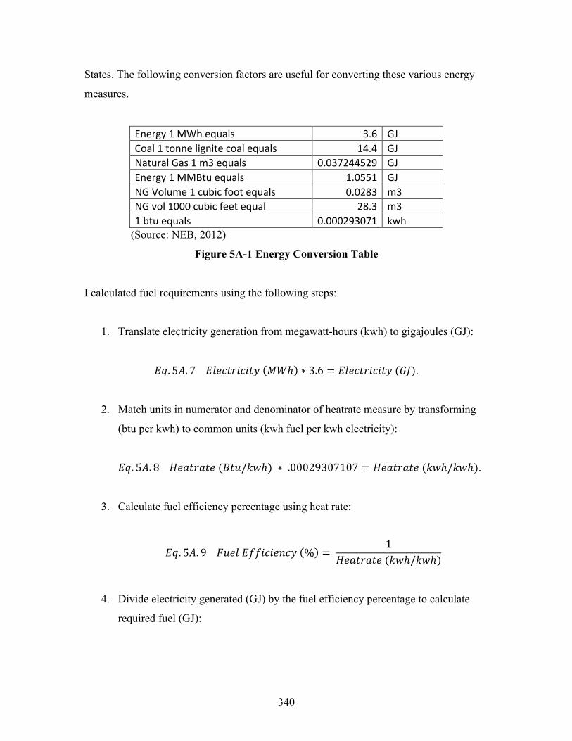
340

States. The following conversion factors are useful for converting these various energy

measures.

Energy1MWhequals 3.6 GJCoal1tonnelignitecoalequals 14.4 GJNaturalGas1m3equals 0.037244529 GJEnergy1MMBtuequals 1.0551 GJNGVolume1cubicfootequals 0.0283 m3NGvol1000cubicfeetequal 28.3 m31btuequals 0.000293071 kwh

(Source: NEB, 2012)

Figure 5A-1 Energy Conversion Table

I calculated fuel requirements using the following steps:

1. Translate electricity generation from megawatt-hours (kwh) to gigajoules (GJ):

𝐸𝑞. 5𝐴. 7 𝐸𝑙𝑒𝑐𝑡𝑟𝑖𝑐𝑖𝑡𝑦 𝑀𝑊ℎ ∗ 3.6 = 𝐸𝑙𝑒𝑐𝑡𝑟𝑖𝑐𝑖𝑡𝑦 (𝐺𝐽).

2. Match units in numerator and denominator of heatrate measure by transforming

(btu per kwh) to common units (kwh fuel per kwh electricity):

𝐸𝑞. 5𝐴. 8 𝐻𝑒𝑎𝑡𝑟𝑎𝑡𝑒 (𝐵𝑡𝑢/𝑘𝑤ℎ) ∗ .00029307107 = 𝐻𝑒𝑎𝑡𝑟𝑎𝑡𝑒 (𝑘𝑤ℎ/𝑘𝑤ℎ).

3. Calculate fuel efficiency percentage using heat rate:

𝐸𝑞. 5𝐴. 9 𝐹𝑢𝑒𝑙 𝐸𝑓𝑓𝑖𝑐𝑖𝑒𝑛𝑐𝑦 % = 1

𝐻𝑒𝑎𝑡𝑟𝑎𝑡𝑒 (𝑘𝑤ℎ/𝑘𝑤ℎ)

4. Divide electricity generated (GJ) by the fuel efficiency percentage to calculate

required fuel (GJ):

341

𝐸𝑞. 5𝐴. 10 𝐹𝑢𝑒𝑙 𝑅𝑒𝑞𝑢𝑖𝑟𝑒𝑑 (𝐺𝐽)! = 𝐸𝑙𝑒𝑐𝑡𝑟𝑖𝑐𝑖𝑡𝑦 (𝐺𝐽)!

𝐹𝑢𝑒𝑙 𝐸𝑓𝑓𝑖𝑐𝑖𝑒𝑛𝑐𝑦 (%)

5. Calculate the cost of the fuel bill. For fuels like natural gas, gigajoules (GJ) are a

convenient unit of measurement. Natural gas prices are often listed in terms of

$/GJ, at least in Canadian data. For other fuels, like coal or uranium, conversions

may be needed, depending on the original data source. In general the fuel bill is

calculated as follows:

𝐸𝑞. 5𝐴. 11 𝐹𝑢𝑒𝑙 𝐵𝑖𝑙𝑙! = 𝐹𝑢𝑒𝑙 𝑅𝑒𝑞𝑢𝑖𝑟𝑒𝑑 (𝑢𝑛𝑖𝑡𝑠)! ∗ 𝐹𝑢𝑒𝑙𝑃𝑟𝑖𝑐𝑒 ($/𝑢𝑛𝑖𝑡)!

Note the time subscripts in equation 5A.9. These allow for the possibility that fuel prices

are not constant over time. The LCOE measures presented in Chapter 5 assume constant

fuel prices. However, fuel prices generally escalate over time. In the linear programming

model (see chapter 7) natural gas prices are allowed to increase over time. Forecasts of

natural gas price increases are taken from the National Energy Board (2013) Energy

Forecast for Canada from 2015 to 2035. Forecasts for natural gas are then extended by

continuing to increase natural gas prices at the annual rate of increase recording during

the period of 2030-2035 in the forecast. The linear programming model also assumes that

coal prices escalate at 1.25%/year (constant 2014 $CAN dollars). Conversations with

relevant experts have indicated that 1.25%/year is an appropriate number for coal price

escalation (Workshop 1).

Capital Cost and Financing Cost Calculation

The installed capital cost of a given electricity generation project can be found by

multiplying the cost per kilowatt installed by the size of the planned installation:

𝐸𝑞. 5𝐴. 12 𝐶𝑎𝑝𝑖𝑡𝑎𝑙 𝐶𝑜𝑠𝑡! = 𝐶𝑜𝑠𝑡 𝑝𝑒𝑟 𝑘𝑖𝑙𝑜𝑤𝑎𝑡𝑡! ∗ 𝑆𝑖𝑧𝑒 (𝑘𝑤)

342

The method of financing the installation of an electricity generation project is another

important part of the cost. There are many different ways to finance capital projects. The

Lazard 8.0 (2014) calculations of LCOE assume the following financing structure:

• 40% equity-financed at 12% return;

• 60% debt-financed at 8%/year interest.

In my calculations of LCOE I assume that 100% of the capital cost is debt-financed at

4%/yr compounding interest. This is a debt-structure that is consistent with SaskPower’s

operations. I calculate financing costs using a monthly periodic interest rate:

𝐸𝑞. 5𝐴. 13 𝑃𝑒𝑟𝑖𝑜𝑑𝑖𝑐 𝐼𝑛𝑡𝑒𝑟𝑒𝑠𝑡 𝑅𝑎𝑡𝑒 𝑖 = (1 + 𝐴𝑛𝑛𝑢𝑎𝑙 𝐼𝑛𝑡𝑒𝑟𝑒𝑠𝑡 𝑅𝑎𝑡𝑒)!/!"

= 𝐴𝑛𝑛𝑢𝑎𝑙 𝐼𝑛𝑡𝑒𝑟𝑒𝑠𝑡 𝑅𝑎𝑡𝑒!"

During the period of construction, interest is charged on the amount of capital required to

construct the project. These interest payments are accumulated during the construction

period, added to the principle, and then capitalized using debt-financing. Pre-

commissioning interest on the amount borrowed is calculated as follows,

𝐸𝑞. 5𝐴. 14 𝐼𝑛𝑡𝑒𝑟𝑒𝑠𝑡 𝐷𝑢𝑟𝑖𝑛𝑔 𝐶𝑜𝑛𝑠𝑡𝑟𝑢𝑐𝑡𝑖𝑜𝑛 (𝐼𝐷𝐶) = 𝑐 ∗ 𝑖 ∗ 𝐶𝑎𝑝𝑖𝑡𝑎𝑙 𝐶𝑜𝑠𝑡!

Where c refers to the number of months of construction and i is the periodic interest rate.

Note that interest charged during the construction period is not compounding, but

accumulates and is amortized upon commissioning.

This approach to interest during construction is meant to mirror SaskPower’s practices.

SaskPower’s policy on capitalizing interest reads as follows:

“Where construction or development of a capital project is ongoing for a

period of time, the asset is not of any productive use to the Corporation,

but funds that could be used elsewhere are being tied up by the

343

construction process. To recognize this inherent carrying cost, interest

must be capitalized on projects that are anticipated to be under

construction or development for a period of 6 months or longer. Interest is

not capitalized on projects that are under construction or development for

less than 6 months.” (SaskPower, 2011: 7)

The costs that are eligible for interest are treated in the following manner:

• “Interest is applied monthly on the ending asset under construction balance –

excluding previously accumulating interest charges” (SaskPower, 2011: 7);

• “The annual interest capitalized during construction is calculated at a simple

interest rate based on the previous year’s weighted average cost of long-term debt

and short-term borrowings” (SaskPower, 2011: 7).

To calculate annual amortized capital costs I assume an amortization period equal to the

lifetime of the technology (measured in years n). Annual amortization payments are then

calculated using this amortization formula:

𝐸𝑞. 5𝐴. 15 𝑀𝑜𝑛𝑡ℎ𝑙𝑦 𝑃𝑎𝑦𝑚𝑒𝑛𝑡 = (𝑃𝑟𝑖𝑛𝑐𝑖𝑝𝑎𝑙 + 𝐼𝐷𝐶) ∗ 𝑖

1− (1+ 𝑖)!!

Where m equals the number of months in the amortization period, which is found by

multiplying the number of years (n) by twelve. Annual capital payments are equal to:

𝐸𝑞. 5𝐴. 16 𝐴𝑛𝑛𝑢𝑎𝑙 𝐶𝑎𝑝𝑖𝑡𝑎𝑙 𝑃𝑎𝑦𝑚𝑒𝑛𝑡! = 𝑀𝑜𝑛𝑡ℎ𝑙𝑦 𝑃𝑎𝑦𝑚𝑒𝑛𝑡!"

!

Operations & Maintenance Costs

Once electricity generation numbers are calculated it is straightforward to calculate

variable operations and maintenance (O&M) costs:

344

𝐸𝑞. 5𝐴. 17 𝑉𝑎𝑟𝑖𝑎𝑏𝑙𝑒 𝑂&𝑀 𝐶𝑜𝑠𝑡 ($)!= 𝑉𝑎𝑟𝑖𝑎𝑏𝑙𝑒𝑂&𝑀 ($/𝑀𝑊ℎ)! ∗ 𝐸𝑙𝑒𝑐𝑡𝑟𝑖𝑐𝑖𝑡𝑦 (𝑀𝑊ℎ)!

Fixed O&M costs are calculated simply in the following way:

𝐸𝑞. 5𝐴. 18 𝐹𝑖𝑥𝑒𝑑 𝑂&𝑀 𝐶𝑜𝑠𝑡 ($)! = 𝐹𝑖𝑥𝑒𝑑𝑂&𝑀 ($/𝑘𝑤/𝑦𝑟)! ∗ 𝐶𝑎𝑝𝑖𝑡𝑎𝑙 (𝑀𝑊)!

Average electricity cost is then calculated by adding up the following:

𝐸𝑞. 5𝐴. 19 𝐴𝑣𝑒𝑟𝑎𝑔𝑒 𝐴𝑛𝑛𝑢𝑎𝑙 𝐶𝑜𝑠𝑡!= 𝐹𝑖𝑥𝑒𝑑 𝑂&𝑀 𝐶𝑜𝑠𝑡! + 𝑉𝑎𝑟𝑖𝑎𝑏𝑙𝑒 𝑂&𝑀 𝐶𝑜𝑠𝑡!+ 𝐴𝑛𝑛𝑢𝑎𝑙 𝐶𝑎𝑝𝑖𝑡𝑎𝑙 𝑃𝑎𝑦𝑚𝑒𝑛𝑡! + 𝐹𝑢𝑒𝑙 𝐵𝑖𝑙𝑙!

Note that this does not include charges for GHG emissions. If a policy path included a

carbon price then additional costs would be added to the average annual cost. The LCOE

numbers in Figure 5-10 do not assign a cost for GHG emissions.

345

References for Appendix 5A

Branker, K., M.J.M. Pathak, and J.M. Pearce (2011). “A review of solar photovoltaic

levelized cost of electricity.” Renewable and Sustainable Energy Reviews. 15, pp. 4470-

4482.

Citi GPS (Global Perspectives & Solutions) (2015) Energy Darwinism II: Why a Low

Carbon Future Doesn’t Have to Cost the Earth. Citigroup. Available on-line at:

https://www.citivelocity.com/citigps/ReportSeries.action?recordId=41. Last accessed

August 20, 2015.

EIA (Energy Information Administration) (2015). Assumptions to the 2015 Annual

Energy Outlook – Table 8.2. Available on-line at:

http://www.eia.gov/forecasts/aeo/assumptions/pdf/table_8.2.pdf. Last accessed August

21, 2015.

EPRI (Electric Power Research Insitute) (2013) Program on Technology Innovation:

Integrated Generation Technology Options 2012. Working Paper #1026656. Palo Alto,

CA: EPRI. Available on-line at:

http://www.epri.com/abstracts/Pages/ProductAbstract.aspx?ProductId=00000000000102

6656. Last accessed August 19, 2015.

Lazard (2014) Lazard’s Levelized Cost of Energy Analysis – Version 8.0. Available on-

line at: http://www.lazard.com/media/1777/levelized_cost_of_energy_-_version_80.pdf.

Last accessed August 17, 2015.

National Energy Board (NEB). (2013). Canada’s Energy Future 2013: Energy Supply

and Demand Projections to 2035. Ottawa, ON: National Energy Board.

346

NEB (2012) Engineering Conversion Tables. Available on-line at: http://www.neb-

one.gc.ca/clf-nsi/rnrgynfmtn/sttstc/nrgycnvrsntbl/nrgycnvrsntbl-eng.html#s4ss6. Last

accessed August 17, 2015.

SaskPower (2015) Investing for our Power Future: 2014 Annual Report. Regina, SK:

SaskPower.

SaskPower (2011) Capitalization Policy. Regina, SK: SaskPower.

Short, Walter, Daniel J. Packey, and Thomas Holt (1995) A Manual for the Economic

Evaluation of Energy Efficiency and Renewable Energy Technologies. Golden, CO:

National Renewable Energy Laboratory (NREL).

347

Appendix 7A – Technical Documentation for the

Saskatchewan Investment Model (SIM)

Introduction

The Saskatchewan Investment Model (SIM) is a linear programming model of the

Saskatchewan electricity sector. The model was built in Excel for Mac 2010 and solved

using the ‘Solver’ optimization tool (Frontline Solvers, 2014). In creating a linear

programming (LP) model it is necessary to specify three components of the model:

1. The objective function defines the value to be minimized or maximized;

2. The decision variables are values that can be increased or decreased in order to

change the value of the objective function;

3. Constraints are necessary to define the problem and restrict the feasible solution

space.

Objective Function

SIM optimizes investment decisions taken in five-year time-steps beginning in 2016-

2020 and ending in 2046-2050. The objective function is defined as the total discounted

cost of supplying electricity over the period (Eq. 7A.1). SIM minimizes 𝐶(𝐼!") by

selecting appropriate investments (𝐼!") in each five-year time-step.

𝐸𝑞. 7𝐴. 1 min𝐶(𝐼!")

= 𝐴𝑛𝑛𝑢𝑎𝑙𝐾𝐶𝑜𝑠𝑡!" + 𝑂&𝑀!" + 𝐹𝑢𝑒𝑙𝐵𝑖𝑙𝑙!" + 𝐶𝑎𝑟𝑏𝑜𝑛𝑡𝑎𝑥 ∗ 𝑁𝑒𝑡𝐺𝐻𝐺𝑠!"

(1+ 𝑟)!

!"

!!!

!

!!!

Where,

• i is a subscript indicating electricity technologies, which include generation

technologies, demand side management measures in the residential, commercial

and industrial sectors, one electricity storage technology, and one technology to

represent contracts for imported hydroelectricity from Manitoba Hydro;

348

• t is a subscript indicating time. There are seven five-year time steps in SIM

representing five-year investment periods beginning in 2016-2020 and ending in

2046-2050. Values in each time-step are assumed to be representative of a five-

year average within that time-step. This means that average values are counted

five times, but are discounted by a discount factor corresponding to the specific

year they are incurred. For example, the average values in the 2020 time-step

would be discounted at t=1, t=2, t=3, t=4 and t=5 and added to the cost total;

• 𝐶 refers to a cost (𝐶) function;

• 𝐼 stands for investment;

• 𝐴𝑛𝑛𝑢𝑎𝑙𝐾𝐶𝑜𝑠𝑡 refers to the annual payment made to cover the cost of capital

investments. Capital is amortized over its lifetime in the same manner outlined in

Equations 5A.12 to 5A.16 in Appendix 5A. I assume an annual interest rate of 4%

for debt-based capital financing costs;

• 𝑂&𝑀 refers to operations and maintenance expenditures and is the sum of fixed

(𝐹𝑖𝑥𝑒𝑑𝑂&𝑀) and variable (𝑉𝑎𝑟𝑖𝑎𝑏𝑙𝑒𝑂&𝑀) O&M expenditures. These are

calculated in the same manner as shown in Equations 5A.17 and 5A.18 in

Appendix 5A;

• 𝐹𝑢𝑒𝑙𝐵𝑖𝑙𝑙 is the cost of purchasing natural gas, coal, biomass and uranium. It is

calculated in the same manner as shown in Equations 5A.7 to 5A.11 in Appendix

5A. In SIM, however, fuel prices are not static and so 𝐹𝑢𝑒𝑙𝑃𝑟𝑖𝑐𝑒 ($/𝑢𝑛𝑖𝑡)! varies

with each time-step (Table 7A.1);

• 𝐶𝑎𝑟𝑏𝑜𝑛𝑡𝑎𝑥 refers to a tax on greenhouse gas emissions, measured in $CAN per

tonne carbon dioxide equivalent (CO2e). A carbon tax can be assigned in the

model to impact optimization decisions. In creating the scenarios in Chapter 7 I

did not assume a carbon price (Carbontax=0). Carbon prices could be selected by

participants in the modelling workshops who used iSIM (see Chapter 9);

• 𝑁𝑒𝑡𝐺𝐻𝐺𝑠 refers to direct greenhouse gas emissions resulting from electricity

generation (measured in tonnes of CO2e) that are released to the atmosphere.

Emissions captured using carbon capture and storage technology are not charged

a carbon tax; and

• 𝑟 is the discount rate.

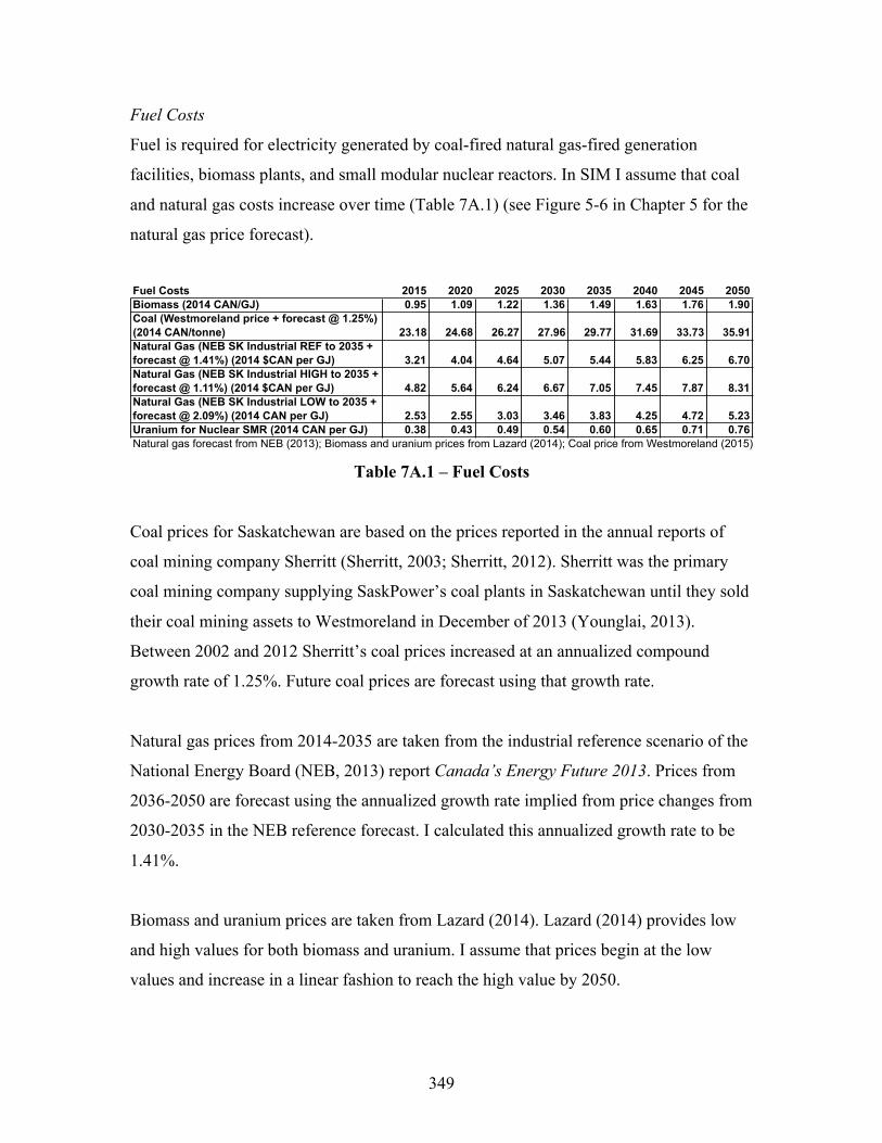
349

Fuel Costs

Fuel is required for electricity generated by coal-fired natural gas-fired generation

facilities, biomass plants, and small modular nuclear reactors. In SIM I assume that coal

and natural gas costs increase over time (Table 7A.1) (see Figure 5-6 in Chapter 5 for the

natural gas price forecast).

Table 7A.1 – Fuel Costs

Coal prices for Saskatchewan are based on the prices reported in the annual reports of

coal mining company Sherritt (Sherritt, 2003; Sherritt, 2012). Sherritt was the primary

coal mining company supplying SaskPower’s coal plants in Saskatchewan until they sold

their coal mining assets to Westmoreland in December of 2013 (Younglai, 2013).

Between 2002 and 2012 Sherritt’s coal prices increased at an annualized compound

growth rate of 1.25%. Future coal prices are forecast using that growth rate.

Natural gas prices from 2014-2035 are taken from the industrial reference scenario of the

National Energy Board (NEB, 2013) report Canada’s Energy Future 2013. Prices from

2036-2050 are forecast using the annualized growth rate implied from price changes from

2030-2035 in the NEB reference forecast. I calculated this annualized growth rate to be

1.41%.

Biomass and uranium prices are taken from Lazard (2014). Lazard (2014) provides low

and high values for both biomass and uranium. I assume that prices begin at the low

values and increase in a linear fashion to reach the high value by 2050.

Fuel Costs 2015 2020 2025 2030 2035 2040 2045 2050Biomass (2014 CAN/GJ) 0.95 1.09 1.22 1.36 1.49 1.63 1.76 1.90Coal (Westmoreland price + forecast @ 1.25%) (2014 CAN/tonne) 23.18 24.68 26.27 27.96 29.77 31.69 33.73 35.91Natural Gas (NEB SK Industrial REF to 2035 + forecast @ 1.41%) (2014 $CAN per GJ) 3.21 4.04 4.64 5.07 5.44 5.83 6.25 6.70Natural Gas (NEB SK Industrial HIGH to 2035 + forecast @ 1.11%) (2014 $CAN per GJ) 4.82 5.64 6.24 6.67 7.05 7.45 7.87 8.31Natural Gas (NEB SK Industrial LOW to 2035 + forecast @ 2.09%) (2014 CAN per GJ) 2.53 2.55 3.03 3.46 3.83 4.25 4.72 5.23Uranium for Nuclear SMR (2014 CAN per GJ) 0.38 0.43 0.49 0.54 0.60 0.65 0.71 0.76Natural gas forecast from NEB (2013); Biomass and uranium prices from Lazard (2014); Coal price from Westmoreland (2015)

350

Greenhouse Gas Emissions

Annual greenhouse gas emissions (GHGs) for each time step are calculated using by

multiplying the natural gas and coal required to generate electricity in that time step

against the GHG intensity of the fuels, measured in CO2e (Equation 7A.2).

𝐸𝑞. 7𝐴. 2 𝐺𝐻𝐺𝑠!"= 𝐹𝑢𝑒𝑙𝑅𝑒𝑞𝑢𝑖𝑟𝑒𝑑(𝐺𝐽/𝐺𝑊ℎ)!" ∗ 𝐸𝑙𝑒𝑐𝑡𝑟𝑖𝑐𝑖𝑡𝑦(𝐺𝑊ℎ)!" ∗ 𝐺𝐻𝐺𝐼𝑛𝑡𝑒𝑛𝑠𝑖𝑡𝑦!

Where,

• j is a subscript indicating fuel type (j ∈ 1,2 where 1 = natural gas, 2 = coal);

• 𝐹𝑢𝑒𝑙𝑅𝑒𝑞𝑢𝑖𝑟𝑒𝑑(𝐺𝐽/𝐺𝑊ℎ)!" indicates the fuel efficiency of each technology. For

coal fuel use gigajoules (GJ) are converted to metric tonnes;

• 𝐸𝑙𝑒𝑐𝑡𝑟𝑖𝑐𝑖𝑡𝑦(𝐺𝑊ℎ)!" is the total amount of electricity generated by fossil-fuel

technology i in time-step t;

• 𝐺𝐻𝐺𝐼𝑛𝑡𝑒𝑛𝑠𝑖𝑡𝑦! is the GHG intensity per unit of fuel expressed in kg CO2e per GJ

for natural gas and tonnes CO2e per tonne for lignite coal.

GHG intensities used in this paper are: 1.46 tonnes CO2e per tonne lignite coal (the coal

burned for electricity production in Saskatchewan is entirely lignite coal); and 49.51

kilograms of CO2e per Gigajoule (GJ) natural gas (Environment Canada, 2014 Part 2 pp.

183-187).

Capital Stock Model

SIM is a capital-stock model. Capital in the model is created through investment,

maintained for its expected lifetime, and retired at the end of its expected lifetime.

Equation 7A.3 shows that the capital stock for any given technology in time-step t

(𝐾!") is equal to the capital stock in the previous time-step (𝐾!,(!!!)) plus investment (𝐼!")

and minus retirements (𝑅!"),

𝐸𝑞. 7𝐴. 3 𝐾!" = 𝐾!,(!!!) + 𝐼!" − 𝑅!" .

351

The capital stock determines the amount of electricity generated (𝐸𝑞. 7𝐴. 4, which is the

same as 𝐸𝑞. 5𝐴. 3 in Appendix 5A). For electricity generation technologies, the capital

stock (𝐾!", measured in MW) is multiplied by its (𝐶𝑎𝑝𝑎𝑐𝑖𝑡𝑦 𝐹𝑎𝑐𝑡𝑜𝑟!") and also the

number of hours in a year (8760) to determine the quantity of electricity generated

(𝐸𝑙𝑒𝑐𝑡𝑟𝑖𝑐𝑖𝑡𝑦!", measured in MWh),

𝐸𝑞. 7𝐴. 4 𝐸𝑙𝑒𝑐𝑡𝑟𝑖𝑐𝑖𝑡𝑦!" = 𝐾!" ∗ 𝐶𝑎𝑝𝑎𝑐𝑖𝑡𝑦 𝐹𝑎𝑐𝑡𝑜𝑟!" ∗ 8760.

I assume that electricity generation technologies produce electricity at their average

𝐶𝑎𝑝𝑎𝑐𝑖𝑡𝑦 𝐹𝑎𝑐𝑡𝑜𝑟!" throughout their lifetime. The capacity factor indicates the

relationship between electricity generated by a technology over the course of a period of

time and the theoretical maximum the technology could have generated in that period of

time (See 𝐸𝑞. 5𝐴. 4 and 𝐸𝑞. 5𝐴. 5). In SIM the capacity factors translate megawatts

(MW) of installed capacity into Megawatt-hours (MWh) of electricity generated (See

𝐸𝑞. 7𝐴. 3). Capacity factors range from a high of 83% for biomass and small, modular

nuclear reactors to lows of 10% for solar thermal and 16% for solar photovoltaic

installations. Due to its strong wind resource, Saskatchewan wind installations are able to

achieve a capacity factor of 37.5%, which is quite high relative to other regions

(Interview 5).

By assuming constant capacity factors the model remains linear. A variation to the model

would allow capacity factors to vary. This could increase the realism of the model, but

would introduce a non-linearity as SIM would have to choose both the capital investment

and the capacity for each technology. Electricity generation for each technology would

then be a multiplicative relationship between two decision variables. For computational

ease, and to ensure the interactive SIM (iSIM) can run in Excel, I have kept relationships

in the model linear.

Decision Variables

The decision variables in SIM are physical capacity investments (measured in megawatts

– MW) in twelve competing electricity generation technologies and one electricity

352

storage technology, as well as demand side management (DSM) efforts (measured in

GWh/yr saved) in three sectors: residential, commercial, and industrial. Investment

decisions are made at five-year intervals beginning in the 2016-2020 interval and

continuing until the 2046-2050 interval.

Electricity Generation Technologies

The twelve electricity generation technologies represented in the model are:

• Biomass

• Conventional coal-fired generation

• Coal-fired generation equipped with carbon capture and storage (CCS)

• Hydroelectric facilities in Saskatchewan

• Hydroelectric capacity purchased from Manitoba Hydro

• Natural gas combined cycle turbines

• Natural gas simple cycle turbines

• Natural gas combined cycle turbines equipped with CCS

• Small, modular nuclear reactors

• Solar – photovoltaic (PV) installations

• Solar concentrating thermal stations

• Wind generation facilities

Investment in each technology is made in terms of megawatts (MW). The capital costs

vary for each technology and also change over time in response to an ‘Autonomous

Capital Cost Improvement’ (ACCI) factor (See Table 5-1). I use Equation 5.1 to model

cost improvement. It is reproduced here as Equation 7A.5,

𝐸𝑞. 7𝐴. 5 𝐶𝑜𝑠𝑡! = 𝐶𝑜𝑠𝑡! ∗ 𝑒𝑥𝑝!!".

This cost improvement equation is also used to calculate cost improvements for fixed

O&M costs (𝐹𝑖𝑥𝑒𝑑𝑂&𝑀) and variable O&M costs (𝑉𝑎𝑟𝑖𝑎𝑏𝑙𝑒𝑂&𝑀). The autonomous

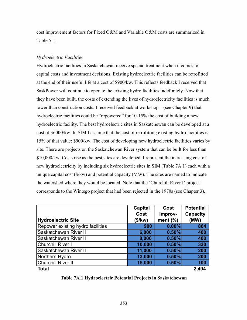
353

cost improvement factors for Fixed O&M and Variable O&M costs are summarized in

Table 5-1.

Hydroelectric Facilities

Hydroelectric facilities in Saskatchewan receive special treatment when it comes to

capital costs and investment decisions. Existing hydroelectric facilities can be retrofitted

at the end of their useful life at a cost of $900/kw. This reflects feedback I received that

SaskPower will continue to operate the existing hydro facilities indefinitely. Now that

they have been built, the costs of extending the lives of hydroelectricity facilities is much

lower than construction costs. I received feedback at workshop 1 (see Chapter 9) that

hydroelectric facilities could be “repowered” for 10-15% the cost of building a new

hydroelectric facility. The best hydroelectric sites in Saskatchewan can be developed at a

cost of $6000/kw. In SIM I assume that the cost of retrofitting existing hydro facilities is

15% of that value: $900/kw. The cost of developing new hydroelectric facilities varies by

site. There are projects on the Saskatchewan River system that can be built for less than

$10,000/kw. Costs rise as the best sites are developed. I represent the increasing cost of

new hydroelectricity by including six hydroelectric sites in SIM (Table 7A.1) each with a

unique capital cost ($/kw) and potential capacity (MW). The sites are named to indicate

the watershed where they would be located. Note that the ‘Churchill River I’ project

corresponds to the Wintego project that had been rejected in the 1970s (see Chapter 3).

Table 7A.1 Hydroelectric Potential Projects in Saskatchewan

Hydroelectric Site

Capital Cost

($/kw)

Cost Improv-

ment (%)

Potential Capacity

(MW)Repower existing hydro facilities 900 0.00% 864 Saskatchewan River II 6,000 0.50% 400 Saskatchewan River II 8,000 0.50% 400 Churchill River I 10,000 0.50% 330 Saskatchewan River II 11,000 0.50% 200 Northern Hydro 13,000 0.50% 200 Churchill River II 15,000 0.50% 100 Total 2,494

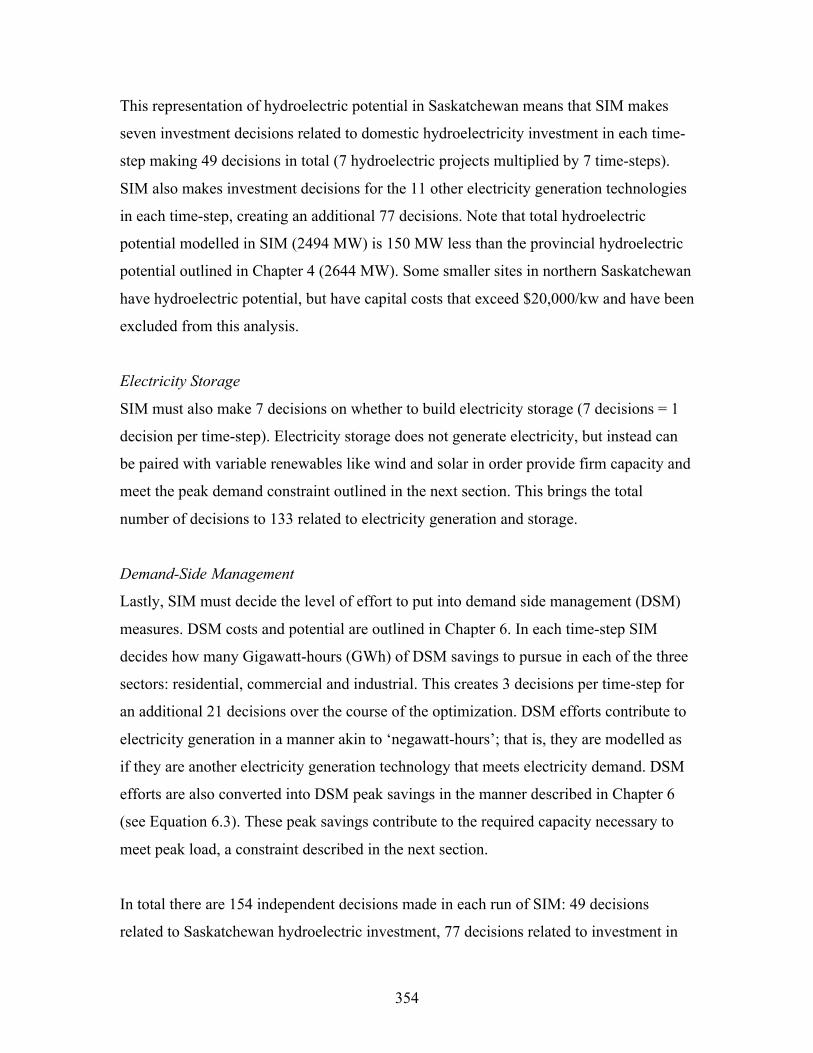
354

This representation of hydroelectric potential in Saskatchewan means that SIM makes

seven investment decisions related to domestic hydroelectricity investment in each time-

step making 49 decisions in total (7 hydroelectric projects multiplied by 7 time-steps).

SIM also makes investment decisions for the 11 other electricity generation technologies

in each time-step, creating an additional 77 decisions. Note that total hydroelectric

potential modelled in SIM (2494 MW) is 150 MW less than the provincial hydroelectric

potential outlined in Chapter 4 (2644 MW). Some smaller sites in northern Saskatchewan

have hydroelectric potential, but have capital costs that exceed $20,000/kw and have been

excluded from this analysis.

Electricity Storage

SIM must also make 7 decisions on whether to build electricity storage (7 decisions = 1

decision per time-step). Electricity storage does not generate electricity, but instead can

be paired with variable renewables like wind and solar in order provide firm capacity and

meet the peak demand constraint outlined in the next section. This brings the total

number of decisions to 133 related to electricity generation and storage.

Demand-Side Management

Lastly, SIM must decide the level of effort to put into demand side management (DSM)

measures. DSM costs and potential are outlined in Chapter 6. In each time-step SIM

decides how many Gigawatt-hours (GWh) of DSM savings to pursue in each of the three

sectors: residential, commercial and industrial. This creates 3 decisions per time-step for

an additional 21 decisions over the course of the optimization. DSM efforts contribute to

electricity generation in a manner akin to ‘negawatt-hours’; that is, they are modelled as

if they are another electricity generation technology that meets electricity demand. DSM

efforts are also converted into DSM peak savings in the manner described in Chapter 6

(see Equation 6.3). These peak savings contribute to the required capacity necessary to

meet peak load, a constraint described in the next section.

In total there are 154 independent decisions made in each run of SIM: 49 decisions

related to Saskatchewan hydroelectric investment, 77 decisions related to investment in

355

11 other electricity generation technologies, 7 decisions related to electricity storage, and

21 decisions related to DSM.

Note that in all but the equivalency scenario conventional coal-fired generation

technologies are not permitted to compete for investment in the model. This

acknowledges the 2012 Canadian coal-fired electricity regulations, which prohibit

investment in electricity generation technologies that emit greenhouse gas emissions in

excess of 420 tonnes carbon dioxide (CO2) emissions per Gigawatt-hour (GWh) of

electricity (CEPA, 2012). This regulation came into effect July 1, 2015 (CEPA, 2012). In

the equivalency scenario it is possible to retrofit existing coal-fired facilities at the end of

their life to extend their longevity. I assume this retrofit option costs $400/kw, a figure

that aligns with Environment Canada’s analysis of the coal-fired regulations (CEPA,

2012).

Constraints

Without constraints, the simplest approach to minimizing the cost of operating the

electricity system would be to sell all of the generation assets and produce zero or even

negative electricity. To motivate a non-trivial solution it is necessary to constrain the

feasible solution set.

Meeting Electricity Demand

The first constraint in the LP model requires that electricity generation is greater or equal

to electricity demand. The forecast for electricity demand used in SIM is presented in

detail in Chapter 6. To match the seven time-steps in the LP model the electricity forecast

has been simplified to seven points (Figure 7A.1).

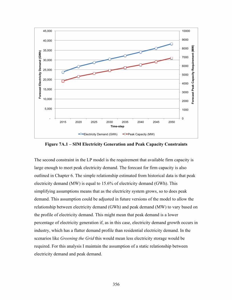
356

Figure 7A.1 – SIM Electricity Generation and Peak Capacity Constraints

The second constraint in the LP model is the requirement that available firm capacity is

large enough to meet peak electricity demand. The forecast for firm capacity is also

outlined in Chapter 6. The simple relationship estimated from historical data is that peak

electricity demand (MW) is equal to 15.6% of electricity demand (GWh). This

simplifying assumptions means that as the electricity system grows, so to does peak

demand. This assumption could be adjusted in future versions of the model to allow the

relationship between electricity demand (GWh) and peak demand (MW) to vary based on

the profile of electricity demand. This might mean that peak demand is a lower

percentage of electricity generation if, as in this case, electricity demand growth occurs in

industry, which has a flatter demand profile than residential electricity demand. In the

scenarios like Greening the Grid this would mean less electricity storage would be

required. For this analysis I maintain the assumption of a static relationship between

electricity demand and peak demand.

0

1000

2000

3000

4000

5000

6000

7000

8000

9000

10000

-

5,000

10,000

15,000

20,000

25,000

30,000

35,000

40,000

45,000

2015 2020 2025 2030 2035 2040 2045 2050

Fore

cast

Pea

k C

apac

ity R

equi

rem

ent (

MW

)

Fore

cast

Ele

ctri

city

Dem

and

(GW

h)

Time-step

Electricity Demand (GWh) Peak Capacity (MW)

357

Firm capacity includes the fossil fuel generation assets (coal- and natural gas-fired

plants), hydroelectric stations, biomass plants, and small modular nuclear reactors. To

allow higher integration of variable renewables, five-eighths of the available electricity

storage capacity is counted towards firm capacity. Wind receives a partial ‘capacity

credit’ in recognition that it is often available; 10% of wind capacity is counted towards

firm capacity (Interview 11). Solar-photovoltaic and solar thermal capacities are not

counted towards the firm capacity total. DSM peak savings are counted as contributing to

firm capacity.

In SIM the retirement schedule for existing electricity generation infrastructure

(presented in Figure 1-3) has also been simplified to seven time steps (Figure 7A.2).

After the optimizations are run I find that existing hydroelectric facilities are maintained

in all scenarios through investments in repowering when retirement is scheduled to occur.

In all but the Greening the Grid scenario, the Shand power plant is retrofitted in 2025 to

extend its life until the 2045 time-step. In the SaskPower BAU scenario Boundary Dam

IV and V are allowed to operate until 2025 when they are then converted to CCS. In all

scenarios, the facilities are retired as scheduled in 2020.

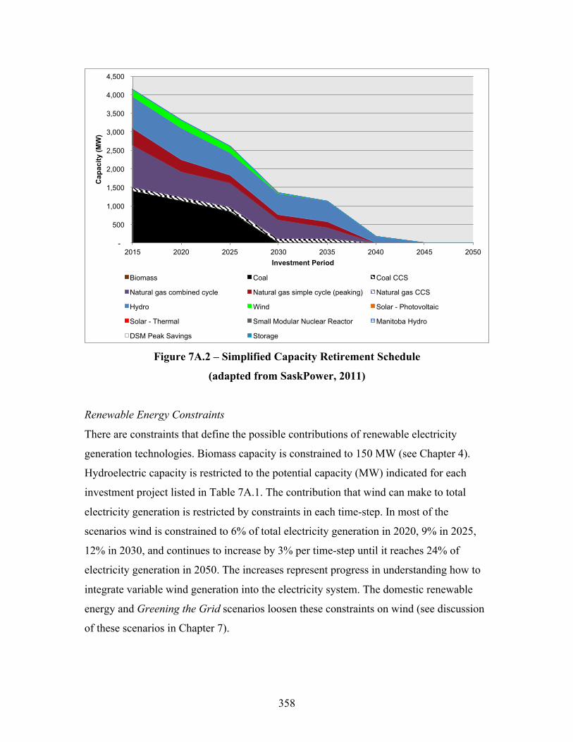
358

Figure 7A.2 – Simplified Capacity Retirement Schedule

(adapted from SaskPower, 2011)

Renewable Energy Constraints

There are constraints that define the possible contributions of renewable electricity

generation technologies. Biomass capacity is constrained to 150 MW (see Chapter 4).

Hydroelectric capacity is restricted to the potential capacity (MW) indicated for each

investment project listed in Table 7A.1. The contribution that wind can make to total

electricity generation is restricted by constraints in each time-step. In most of the

scenarios wind is constrained to 6% of total electricity generation in 2020, 9% in 2025,

12% in 2030, and continues to increase by 3% per time-step until it reaches 24% of

electricity generation in 2050. The increases represent progress in understanding how to

integrate variable wind generation into the electricity system. The domestic renewable

energy and Greening the Grid scenarios loosen these constraints on wind (see discussion

of these scenarios in Chapter 7).

-

500

1,000

1,500

2,000

2,500

3,000

3,500

4,000

4,500

2015 2020 2025 2030 2035 2040 2045 2050

Cap

acity

(MW

)

Investment Period

Biomass Coal Coal CCS

Natural gas combined cycle Natural gas simple cycle (peaking) Natural gas CCS

Hydro Wind Solar - Photovoltaic

Solar - Thermal Small Modular Nuclear Reactor Manitoba Hydro

DSM Peak Savings Storage

359

Electricity Storage Constraint

Electricity storage is constrained to have a value less than or equal to 50% of the total

capacity of the variable renewable technologies: wind, solar-PV, and solar thermal. This

constraint ensures that electricity storage is matched with variable electricity supply. It is

modelled after the relationship found at the Cowessess Wind Battery Storage project,

where an 800-kilowatt (kW) Enercon wind turbine is matched with 400 kW of lithium-

ion battery storage (Jansen, 2014).

Demand Side Management Constraints

Demand side management (DSM) efforts are constrained in each time-step to the

potential outlined in Chapter 6 (see Tables 6-4, 6-5, and 6-6). DSM efforts are reset to

zero in each time-step. This assumes that for energy conservation gains to be maintained,

sustained effort must be put into DSM programming. This is a way of recognizing the

potential for rebound effects following from energy conservation efforts.

Policy Constraints

The greenhouse gas (GHG) emissions reduction scenarios are motivated using

constraints. The equivalency scenario involves constraining GHG emissions in 2020 to be

equal to those achieved in the SaskPower BAU scenario. The four scenarios for reducing

GHG emissions by 80% below 2015 levels by 2050 each constrain GHGs from electricity

to that level. The domestic renewable energy scenario also requires that total electricity

generated by the combination of biomass plants, hydroelectric stations, wind turbines,

solar-PV installations, solar thermal installations, and DSM efforts, equals or exceeds

90% of total electricity generation in 2050.

The third scenario, an escalating carbon tax, does not require an additional constraint.

Instead the carbon tax affects the objective function directly and penalizes fossil fuel

generation options for the GHGs released to the atmosphere. GHG emissions stored

underground through carbon capture and storage (CCS) are not charged a carbon tax.

Emissions that emerge from underground when captured carbon is used to extract oil are

360

also not charged to the electricity system; it is assumed that these GHGs would become a

liability of the fossil fuel extraction sector.

Limitations

Because the linear program is set up to minimize the total discounted operating cost of

meeting Saskatchewan’s electricity demand the relative costs of the various technologies

are important. The linear programming model will select the least cost option that meets

the necessary constraints. This is true even if costs differ only slightly. Linear

programming (LP) models are often critiqued for “penny-switching” (Jaccard et al.,

2003). This means that the LP model will switch from one preferred electricity generation

technology to another even if the costs of the technologies differ by a fraction of a cent

(Jaccard et al., 2003). Because of the importance of relative costs, I conduct a sensitivity

analysis of key cost assumptions in Chapter 7. I also encourage readers not to interpret

the scenarios resulting from SIM as ‘optimal’; the optimization program merely provides

a decision-rule for assembling scenarios at the least financial cost to SaskPower. Chapter

8 explores the impacts of these scenarios that are not easily translated into financial cost.

361

References for Appendix 7A

Canadian Environmental Protection Act (CEPA): Reduction of Carbon Dioxide

Emissions from Coal-fired Generation of Electricity Regulations (2012) Canada Gazette

Part II, 146:19. Retrieved from: http://www.gazette.gc.ca/rp-pr/p2/2012/2012-09-

12/html/sor-dors167-eng.html. Last accessed October 14, 2015.

Environment Canada (2014) National Inventory Report 1990-2012: Greenhouse Gas

Sources and Sinks in Canada. The Canadian Government’s Submission to the UN

Framework Convention on Climate Change. Ottawa, ON: Minister of the Environment.

Frontline Solvers (2014) Solver Excel Add-in. More information on the Solver add-in

available on-line at: http://www.solver.com, Last accessed December 3, 2014.

Jaccard, Mark, Richard Loulou, Amit Kanudia, John Nyboer, Alison Bailie, Maryse

Labriet (2003) “Methodological contrasts in costing greenhouse gas abatement policies:

Optimization and simulation modeling of micro-economic effects in Canada.” European

Journal of Operations Research. 145, pp. 148-164.

Jansen, Ryan (2014) Personal correspondence. August, 2014 at Regina, SK.

Lazard (2014) Lazard’s Levelized Cost of Energy Analysis – Version 8.0. Available on-

line at: http://www.lazard.com/media/1777/levelized_cost_of_energy_-_version_80.pdf.

Last accessed: September 11, 2015.

National Energy Board (NEB) (2013) Canada’s Energy Future 2013: Energy Supply and

Demand Projections to 2035. Ottawa, ON: National Energy Board.

SaskPower (2011) SaskPower’s Electricity and Conservation Strategy for Meeting

Saskatchewan’s Needs. Regina, SK: SaskPower.

362

Sherritt (2013) Annual Report 2013. Sherritt International Corporation. Accessed on-line

at: http://www.sherritt.com/investor-relations/financial-reports/annual-reports, last

accessed December 3, 2014.

Sherritt (2012) Annual Report 2012. Sherritt International Corporation. Accessed on-line

at: http://www.sherritt.com/investor-relations/financial-reports/annual-reports, last

accessed December 3, 2014.

Sherritt (2003) Annual Report 2003. Sherritt International Corporation. Accessed on-line

at: http://www.sherritt.com/investor-relations/financial-reports/annual-reports, last

accessed December 3, 2014.

Younglai, Rachelle (2013) “Major shareholder calls for board shakeup as Sherritt exits

coal.” The Globe and Mail. December 24, 2013. Available on-line at:

http://www.theglobeandmail.com/report-on-business/industry-news/energy-and-

resources/sherritt-to-sell-coal-business-for-946-million/article16097443/, Last accessed

December 3, 2014.

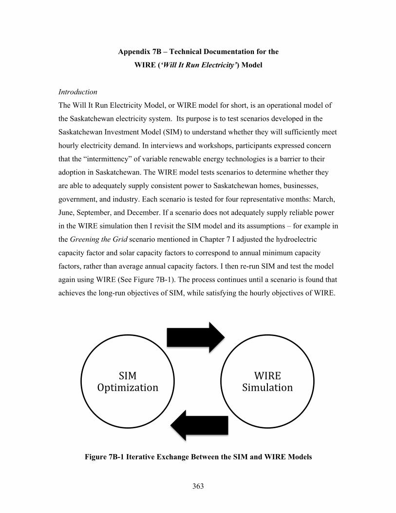
363

Appendix 7B – Technical Documentation for the

WIRE (‘Will It Run Electricity’) Model

Introduction

The Will It Run Electricity Model, or WIRE model for short, is an operational model of

the Saskatchewan electricity system. Its purpose is to test scenarios developed in the

Saskatchewan Investment Model (SIM) to understand whether they will sufficiently meet

hourly electricity demand. In interviews and workshops, participants expressed concern

that the “intermittency” of variable renewable energy technologies is a barrier to their

adoption in Saskatchewan. The WIRE model tests scenarios to determine whether they

are able to adequately supply consistent power to Saskatchewan homes, businesses,

government, and industry. Each scenario is tested for four representative months: March,

June, September, and December. If a scenario does not adequately supply reliable power

in the WIRE simulation then I revisit the SIM model and its assumptions – for example in

the Greening the Grid scenario mentioned in Chapter 7 I adjusted the hydroelectric

capacity factor and solar capacity factors to correspond to annual minimum capacity

factors, rather than average annual capacity factors. I then re-run SIM and test the model

again using WIRE (See Figure 7B-1). The process continues until a scenario is found that

achieves the long-run objectives of SIM, while satisfying the hourly objectives of WIRE.

Figure 7B-1 Iterative Exchange Between the SIM and WIRE Models

SIMOptimization

WIRESimulation

364

Related Literature

The WIRE model builds on the work of Benitez, Benitez and van Kooten (2008) who use

an hourly electricity model to understand the economic impact of increased wind power

penetration in Alberta. Benitez et al. (2008) also consider the economic impact of using

wind in combination with hydroelectric power storage in the province. The formulation

for ramp rate constraints (identified below) is drawn from van Kooten (2012).

Model Description

The WIRE model is a non-linear programming optimization model. It is coded in the

GAMS (General Algebraic Modelling Software) language and solved with a non-linear

programming solver. The GAMS code for this model is included at the end of this

appendix.

The WIRE model is designed to model a one-month time span with hourly (h) time steps.

Months with 30 days have 720 time steps (hours), while months with 31 days have 744

time steps. In each time step electricity generation must be large enough to meet

electricity demand.

Electricity Demand

Hourly electricity demand data and hourly wind power production data for 2013 were

supplied by SaskPower and compiled by Dr. Mark Bigland-Pritchard (2015a). This

hourly data is separated out by ‘power class’, ‘oilfield’, and ‘other’. I scale this hourly

electricity demand for each category to represent the composition of demand in 2050.

There are three scenarios for demand; a business as usual (BAU) scenario where few

demand side management (DSM) actions are taken by 2050, a medium scenario with

greater levels of DSM, and a high scenario that achieves the greatest level of DSM. In the

BAU scenario, power class electricity demand is forecast to grow by a factor of 2.13

from 2015 to 2050. To represent this scenario in WIRE I scale the hourly power class

data from 2013 by multiplying by 2.13. The scaling factors I use for each of the scenarios

and customer categories are as follows:

365

Table 7B.1 Scaling Factors for Electricity Demand

Objective Function

The objective function in WIRE is a cost function that adds up the variable operations

and maintenance costs and fuel costs of operating a given electricity system. The

objective function also includes the capital cost of building an additional natural gas

peaking plant if supply is insufficient to meet demand. The cost function (z) is

represented by the following equation:

𝐸𝑞. 7𝐵. 1 𝐶𝑜𝑠𝑡 𝑧 = 𝑉𝑂𝑀! + 𝐹𝑢𝑒𝑙! ∗ 𝐺𝑒𝑛!,!!!

!! .

In GAMS code, this equation is represented as follows:

cost .. z =e= (sum(h,(sum(i,(VOM(i)+Fuel(i))*(Gen(h,i)))))).

Where,

• h is an index of the number of hours in the month;

• i is an index of electricity generation technologies;

• VOM(i) is the variable operations and maintenance cost per MWh of electricity

generated for technology i;

• Fuel(i) is the fuel cost per MWh of electricity generated for technology i;

• Gen(h,i) is the electricity generated (in MWh) in hour h by technology i;

The summation brackets indicate that the objective function sums variable O&M costs

and fuel costs over each technology (i) for each hour (h). The WIRE model works to

minimize cost by adjusting available decision variables and adhering to constraints

imposed on the model. The WIRE model prioritizes the lowest cost generation options

for each hour.

Customer Type BAU Med. DSM High DSMPower class 2.13 1.99 1.94Oilfield 1.00 0.94 0.92All other 1.47 1.38 1.34

366

Decision Variables

Within the objective function the decision variable is Gen(h,i) which requires the WIRE

model to make h x i decisions to decide how much electricity is generated by each

generation technology (i) in each hour (h).

The WIRE model also contains several other decision variables related to variable

renewable electricity generated by wind and solar, and demand side management peak

shifting opportunities. I explore these below.

Wind Energy

Wind electricity generation in each hour is taken as a given in WIRE. Wind electricity

generation is calculated by multiplying the hourly capacity factors achieved by

Saskatchewan wind turbines in 2013 with installed wind capacity in the given SIM

scenario:

𝐸𝑞. 7𝐵. 2 𝑊𝑖𝑛𝑑𝐺𝑒𝑛! =𝑊𝑖𝑛𝑑𝐶𝑎𝑝 ∗𝑊𝑖𝑛𝑑𝐶𝐹! .

In GAMS code, this equation is represented as:

WindGen(h)=WindCap*WindCF(h).

Where,

• WindGen(h) is the amount of electricity generated in hour (h) by wind turbines in

Saskatchewan;

• WindCap is the total MW of installed capacity of wind power in the province;

• WindCF(h) is the capacity factor in hour (h) of Saskatchewan wind turbines. This

data was obtained from SaskPower by Mark Bigland-Pritchard. It is loaded into

the model as a set of hourly parameters.

367

The optimization model must determine how much wind electricity to use to meet

demand, how much to store for later use, and how much to curtail if production exceeds

demand or the other generation technologies cannot ramp up or down fast enough. These

decisions are represented by the following variables:

• UseWind(h) is a decision variable indicating the amount of wind electricity used

to meet electricity demand in hour h;

• WindStore(h) is a decision variable indicating the level of wind electricity to store

in hour h;

• Curtail(h) is a decision variable indicating the amount of wind electricity to curtail

in hour h;

The sum of these three variables must equal total wind electricity generation

(WindGen(h)). This is represented in WIRE by the following equation:

𝐸𝑞. 7𝐵. 3 𝑊𝑖𝑛𝑑𝐺𝑒𝑛! = 𝑈𝑠𝑒𝑊𝑖𝑛𝑑! +𝑊𝑖𝑛𝑑𝑆𝑡𝑜𝑟𝑒! + 𝐶𝑢𝑟𝑡𝑎𝑖𝑙! .

In GAMS code this is represented by the equation:

Windy(h) .. WindGen(h) =e= Windstore(h) + Usewind(h) + Curtail(h).

Solar Energy

Like wind, solar energy is taken as a given in the WIRE model. Hourly solar photovoltaic

capacity factors for Estevan in 2003 were calculated by Dr. Mark Bigland-Pritchard

(2015b) using data from Environment Canada’s CWEC weather database. Of interest,

these solar capacity factors display significant seasonal variation.

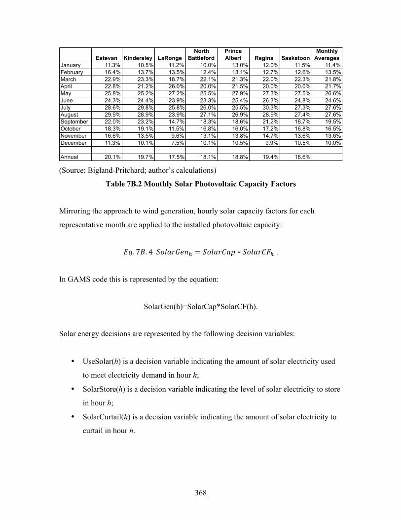
368

(Source: Bigland-Pritchard; author’s calculations)

Table 7B.2 Monthly Solar Photovoltaic Capacity Factors

Mirroring the approach to wind generation, hourly solar capacity factors for each

representative month are applied to the installed photovoltaic capacity:

𝐸𝑞. 7𝐵. 4 𝑆𝑜𝑙𝑎𝑟𝐺𝑒𝑛! = 𝑆𝑜𝑙𝑎𝑟𝐶𝑎𝑝 ∗ 𝑆𝑜𝑙𝑎𝑟𝐶𝐹! .

In GAMS code this is represented by the equation:

SolarGen(h)=SolarCap*SolarCF(h).

Solar energy decisions are represented by the following decision variables:

• UseSolar(h) is a decision variable indicating the amount of solar electricity used

to meet electricity demand in hour h;

• SolarStore(h) is a decision variable indicating the level of solar electricity to store

in hour h;

• SolarCurtail(h) is a decision variable indicating the amount of solar electricity to

curtail in hour h.

Estevan Kindersley LaRongeNorth

BattlefordPrince Albert Regina Saskatoon

Monthly Averages

January 11.3% 10.5% 11.2% 10.0% 13.0% 12.0% 11.5% 11.4%February 16.4% 13.7% 13.5% 12.4% 13.1% 12.7% 12.6% 13.5%March 22.9% 23.3% 18.7% 22.1% 21.3% 22.0% 22.3% 21.8%April 22.8% 21.2% 26.0% 20.0% 21.5% 20.0% 20.0% 21.7%May 25.8% 25.2% 27.2% 25.5% 27.9% 27.3% 27.5% 26.6%June 24.3% 24.4% 23.9% 23.3% 25.4% 26.3% 24.8% 24.6%July 28.6% 29.8% 25.8% 26.0% 25.5% 30.3% 27.3% 27.6%August 29.9% 28.9% 23.9% 27.1% 26.9% 28.9% 27.4% 27.6%September 22.0% 23.2% 14.7% 18.3% 18.6% 21.2% 18.7% 19.5%October 18.3% 19.1% 11.5% 16.8% 16.0% 17.2% 16.8% 16.5%November 16.6% 13.5% 9.6% 13.1% 13.8% 14.7% 13.6% 13.6%December 11.3% 10.1% 7.5% 10.1% 10.5% 9.9% 10.5% 10.0%

Annual 20.1% 19.7% 17.5% 18.1% 18.8% 19.4% 18.6%

369

The sum of these three variables must equal total solar electricity generation

(SolarGen(h)). This is represented in WIRE by the following equation:

𝐸𝑞. 7𝐵. 5 𝑆𝑜𝑙𝑎𝑟𝐺𝑒𝑛! = 𝑈𝑠𝑒𝑆𝑜𝑙𝑎𝑟! + 𝑆𝑜𝑙𝑎𝑟𝑆𝑡𝑜𝑟𝑒! + 𝑆𝑜𝑙𝑎𝑟𝐶𝑢𝑟𝑡𝑎𝑖𝑙! .

In GAMS code this is represented by the equation:

Sunny(h) .. SolarGen(h)=e= SolarStore(h) + UseSolar(h) + SolarCurtail(h).

The WIRE model will choose to store solar electricity in any one hour if it can be used at

a later hour to meet electricity demand and lower total costs for the month. The WIRE

model will choose to curtail solar electricity in any given hour if excess electricity is

being generated at that hour and electricity storage is at full capacity.

Electricity Storage

The possibility of storing electricity has been built into the model in order to address

issues of renewable energy variability. The storage technology resembles the

characteristics of a lithium-ion battery, pumped-hydro storage, or compressed air storage.

Because the model is run within each representative month independently, seasonal

storage is not represented in the model. Future versions of WIRE may improve upon this.

There are three main factors that determine the characteristics of electricity storage in

WIRE:

• Storecap: the capacity of electricity storage in the SIM scenario, expressed in

MW. Efforts are made to iteratively reduce the storage capacity when possible;

• Storage.up: the maximum amount of electricity – expressed in MWh – that can be

held in storage. I assume that a 400 MW electricity storage facility can store 744

MWh of electricity. This relationship is consistent with the Cowessess wind

storage project located east of Regina where a 400-kilowatt lithium-ion battery is

able to store 744 kWh of electricity (personal communication Ryan Jansen, June

370

2014). This relationship is expressed with the following constraint in GAMS:

Storage.up(h) = Storecap * (744/400)

• UseStore(h): is a decision variable determined by the optimization solver. The

WIRE model determines the amount of stored electricity to use in each hour (h).

Importantly, there are conversion losses in the process of storing electricity. To

model these conversion losses, only 70% of the electricity pulled from storage can

be used to meet supply. This represents a 30% conversion loss from storage.

Demand Side Management Peak Shifting

The WIRE model is built to allow peak shifting demand side management (DSM). I

allow electricity demand from one hour (h) to be shifted ahead three hours (h+3). This is

introduced with a simple equality:

𝐸𝑞. 7𝐵. 6 𝐷𝑆𝑀𝑠𝑎𝑣𝑒! = 𝐷𝑆𝑀𝑠𝑝𝑒𝑛𝑑!!! .

In GAMS code, this is represented by:

DSM(h) .. DSMsave(h) =e= DSMspend(h+3);

The WIRE model must then determine how much electricity demand to save in a given

hour (h) in order to shift it ahead three hours. This peak shifting is limited by an upper

bound that corresponds to the peak savings that result in a given SIM scenario. The upper

bound is indicated in GAMS as follows:

• DSMsave.up(h) = 67;

• DSMspend.up(h) = 67.

In this illustrative scenario 67 MW of peak shaving capacity are available.

371

Meeting Supply

The key constraint in the WIRE model is ensuring that electricity demand, net of DSM, is

lesser or equal to electricity generation in each hour. This constraint is characterized as

follows:

𝐸𝑞. 7𝐵. 7 𝐷𝑒𝑚𝑎𝑛𝑑! − 𝐷𝑆𝑀𝑠𝑎𝑣𝑒! + 𝐷𝑆𝑀𝑠𝑝𝑒𝑛𝑑!

≤ 𝐺𝑒𝑛!,!

!

!

+ 𝑈𝑠𝑒𝑊𝑖𝑛𝑑! + 𝑈𝑠𝑒𝑆𝑜𝑙𝑎𝑟! + (.7 ∗ 𝑈𝑠𝑒𝑆𝑡𝑜𝑟𝑒!)

And in GAMS code is represented as:

Meetsupply(h) .. Demand(h) - DSMsave(h) + DSMspend(h) =l= sum(i, (Gen(h,i) )) +

Usewind(h) + UseSolar(h) + .7*Usestore(h) .

Where,

• 𝐷𝑒𝑚𝑎𝑛𝑑! is electricity demand in each hour;

• 𝐺𝑒𝑛!,! is the amount of electricity generated by technology i in hour (h);

• The other factors are as explained above.

Capacity Constraints

I constrain the total contribution that thermal, nuclear, biomass, and hydroelectric

electricity technologies can provide over the course of a month. For the thermal, nuclear,

and biomass technologies, these constraints largely align with the default settings in SIM.

Occasionally, and usually when running WIRE for December when demand is highest, I

allow the capacity constraint for a technology like natural gas combined cycle plants to

achieve a value of 85%. This is a value that can be achieved when a natural gas plant is

running as a source of “baseload” power.

Hydroelectric capacity is limited by seasonal capacity factors. Due to winter snowmelt,

streamflow in Saskatchewan is highest in the late spring. Water storage is available at

Lake Diefenbaker where the Coteau Creek generating station is located. Coteau Creek is

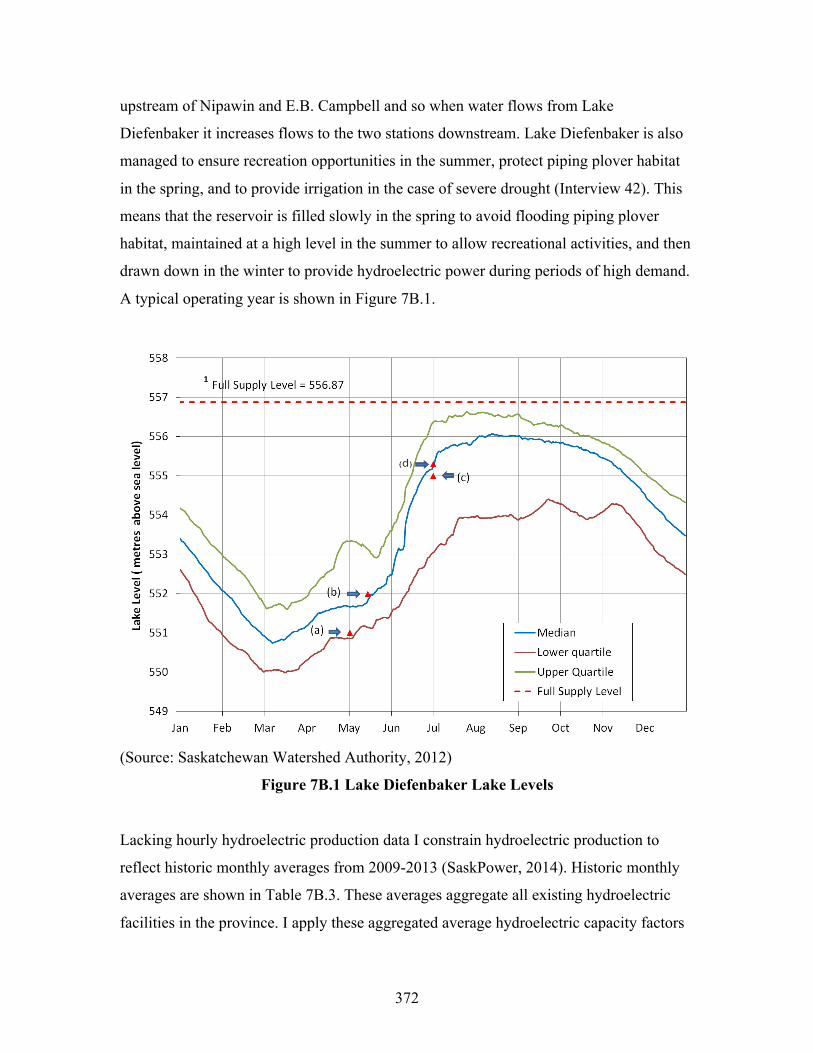
372

upstream of Nipawin and E.B. Campbell and so when water flows from Lake

Diefenbaker it increases flows to the two stations downstream. Lake Diefenbaker is also

managed to ensure recreation opportunities in the summer, protect piping plover habitat

in the spring, and to provide irrigation in the case of severe drought (Interview 42). This

means that the reservoir is filled slowly in the spring to avoid flooding piping plover

habitat, maintained at a high level in the summer to allow recreational activities, and then

drawn down in the winter to provide hydroelectric power during periods of high demand.

A typical operating year is shown in Figure 7B.1.

(Source: Saskatchewan Watershed Authority, 2012)

Figure 7B.1 Lake Diefenbaker Lake Levels

Lacking hourly hydroelectric production data I constrain hydroelectric production to

reflect historic monthly averages from 2009-2013 (SaskPower, 2014). Historic monthly

averages are shown in Table 7B.3. These averages aggregate all existing hydroelectric

facilities in the province. I apply these aggregated average hydroelectric capacity factors

9

Four target elevations for filling Lake Diefenbaker during late spring/early summer have been established to help meet the multiple purposes.

May 1 target elevation of 551.0 m. This elevation is the minimum acceptable level for many of the purposes served; and

May 15 target elevation of 552.0 m. This level is required to launch boats at Elbow Harbour.

July 1 target elevation within the range of 555.0 to 555.3 m. This level provides for summer recreational use.

July 1 target elevation of 555.3 m. This elevation is the maximum level that the reservoir can fill before flooding of significant portions of the Piping Plover nesting habitat occurs. It serves the use of water supply generally while maintaining a level of flood control capacity.

Figure 5: Annual water level fluctuations on Lake Diefenbaker (1980-2009). Lower quartile, upper quartile and median daily water elevations throughout the year. Points plotted represent elevations considered during the operation of Lake Diefenbaker (a) Irrigation minimum (551.0 m); (b) Navigation (552.0 m); (c) Optimal recreation use (555.0 to 555.3); and (d) Maximum for Piping Plover (555.3). *(d) July 1 Piping Plover Target 555.00 to 555.30 metres above sea level is a general guideline for long-term

management. The Draft South Saskatchewan River Piping Plover Conservation Plan also recommends that a water

level increase greater than 3.0m from May 12 to July 1 should be avoided, except under emergency flooding

situations. 1Full supply level is the maximum normal operating level of a reservoir behind a dam. For Lake Diefenbaker the full

supply level is 556.87 m.

1

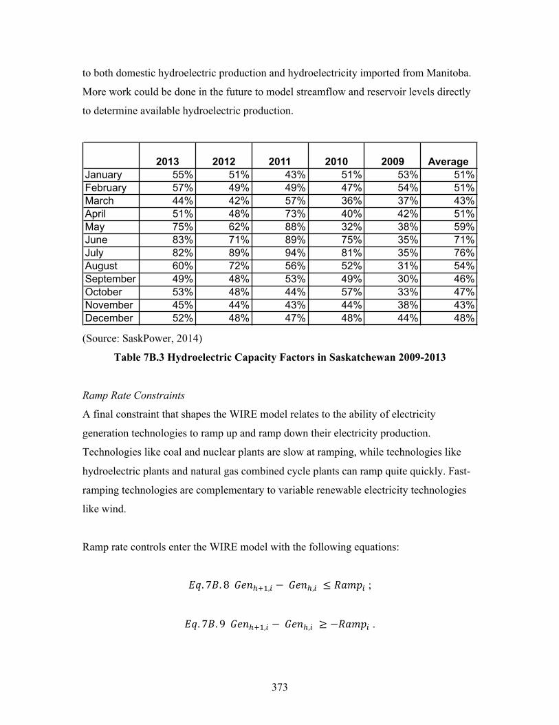
373

to both domestic hydroelectric production and hydroelectricity imported from Manitoba.

More work could be done in the future to model streamflow and reservoir levels directly

to determine available hydroelectric production.

(Source: SaskPower, 2014)

Table 7B.3 Hydroelectric Capacity Factors in Saskatchewan 2009-2013

Ramp Rate Constraints

A final constraint that shapes the WIRE model relates to the ability of electricity

generation technologies to ramp up and ramp down their electricity production.

Technologies like coal and nuclear plants are slow at ramping, while technologies like

hydroelectric plants and natural gas combined cycle plants can ramp quite quickly. Fast-

ramping technologies are complementary to variable renewable electricity technologies

like wind.

Ramp rate controls enter the WIRE model with the following equations:

𝐸𝑞. 7𝐵. 8 𝐺𝑒𝑛!!!,! − 𝐺𝑒𝑛!,! ≤ 𝑅𝑎𝑚𝑝! ;

𝐸𝑞. 7𝐵. 9 𝐺𝑒𝑛!!!,! − 𝐺𝑒𝑛!,! ≥ −𝑅𝑎𝑚𝑝! .

2013 2012 2011 2010 2009 AverageJanuary 55% 51% 43% 51% 53% 51%February 57% 49% 49% 47% 54% 51%March 44% 42% 57% 36% 37% 43%April 51% 48% 73% 40% 42% 51%May 75% 62% 88% 32% 38% 59%June 83% 71% 89% 75% 35% 71%July 82% 89% 94% 81% 35% 76%August 60% 72% 56% 52% 31% 54%September 49% 48% 53% 49% 30% 46%October 53% 48% 44% 57% 33% 47%November 45% 44% 43% 44% 38% 43%December 52% 48% 47% 48% 44% 48%

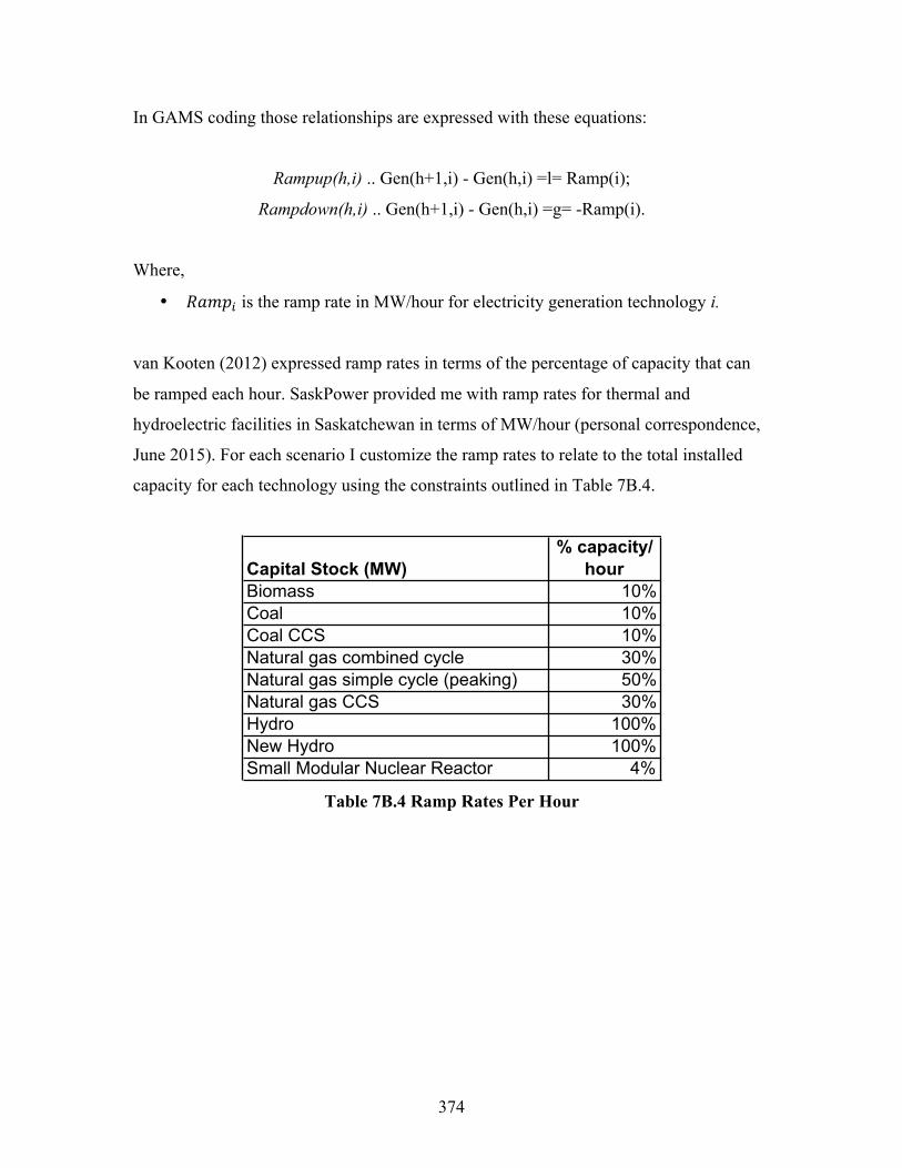
374

In GAMS coding those relationships are expressed with these equations:

Rampup(h,i) .. Gen(h+1,i) - Gen(h,i) =l= Ramp(i);

Rampdown(h,i) .. Gen(h+1,i) - Gen(h,i) =g= -Ramp(i).

Where,

• 𝑅𝑎𝑚𝑝! is the ramp rate in MW/hour for electricity generation technology i.

van Kooten (2012) expressed ramp rates in terms of the percentage of capacity that can

be ramped each hour. SaskPower provided me with ramp rates for thermal and

hydroelectric facilities in Saskatchewan in terms of MW/hour (personal correspondence,

June 2015). For each scenario I customize the ramp rates to relate to the total installed

capacity for each technology using the constraints outlined in Table 7B.4.

Table 7B.4 Ramp Rates Per Hour

Capital Stock (MW)% capacity/

hourBiomass 10%Coal 10%Coal CCS 10%Natural gas combined cycle 30%Natural gas simple cycle (peaking) 50%Natural gas CCS 30%Hydro 100%New Hydro 100%Small Modular Nuclear Reactor 4%

375

References for Appendix 7B

Benitez, Liliana E., Pablo C. Benitez, G. Cornelis van Kooten (2008) “The economics of

wind power with energy storage.” Energy Economics. 30, pp. 1973-1989.

Bigland-Pritchard, Mark (2015a) Hourly Electricity Demand by Customer Category.

Saskatoon, SK: Low-Energy Design.

Bigland-Pritchard, Mark (2015b) Hourly Solar Capacity Factors for 2003 calculated

from Environment Canada’s CWEC weather database. Saskatoon, SK: Low-Energy

Design.

Jansen, Ryan (2014) Personal Correspondence. Meeting at the Cowessess Wind Storage

Demonstration Project, Regina, SK, June 2014.

Saskatchewan Watershed Authority (2012) Developing a New Reservoir Operating Plan

for Lake Diefenbaker. Document Prepared for Consultation Meeting May 30, 2012.

Regina, SK: SWA.

SaskPower (2014) 2014, 2015, 2016 Rate Application: Response to SIECA Second Round

Information Requests. Available on-line at:

http://www.saskratereview.ca/index.php?option=com_content&view=article&id=50&Ite

mid=16. Last accessed October 16, 2015.

van Kooten, G. Cornelis (2012) “Natural Gas, Wind and Nuclear Options for Generating

Electricity in a Carbon Constrained World.” Resource Economics & Policy Analysis

Research Group Working Paper 2012-01. Victoria, BC: University of Victoria

Department of Economics.

376

GAMS Code for the WIRE Model

$Title Will It Run Electricity Model – aka the WIRE model

$Ontext

Scenario: BAU + DSM in March 2050

Version: October 13, 2015

This is a model of the operational characteristics of electricity scenarios generated by the

SIM model. It is built to run over the course of one month and to minimize the cost of

generating electricity over that month.

$Offtext

set

h hours /1*744/ ;

set

i gentype /coal, coal-CCS, NGSC, NGCC, NG-CCS, Hydro, MBHydro, Biomass,

Nuclear, Import /;

Parameters

*The $include command allows data to be imported from a .csv file

D(h) Electricity demand /

$ondelim

$include March2050Demand.csv

$offdelim

/

WindCF(h) Wind capacity factor at each hour in 2013 on SaskPower system /

$ondelim

$include March2050WindCF.csv

$offdelim

/

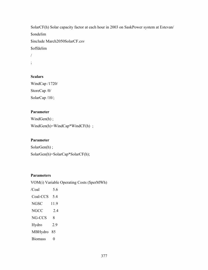
377

SolarCF(h) Solar capacity factor at each hour in 2003 on SaskPower system at Estevan/

$ondelim

$include March2050SolarCF.csv

$offdelim

/

;

Scalars

WindCap /1720/

StoreCap /0/

SolarCap /10/;

Parameter

WindGen(h) ;

WindGen(h)=WindCap*WindCF(h) ;

Parameter

SolarGen(h) ;

SolarGen(h)=SolarCap*SolarCF(h);

Parameters

VOM(i) Variable Operating Costs ($perMWh)

/Coal 5.6

Coal-CCS 5.4

NGSC 11.9

NGCC 2.4

NG-CCS 8

Hydro 2.9

MBHydro 85

Biomass 0

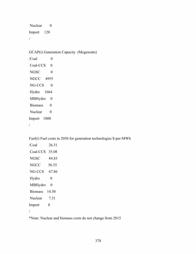
378

Nuclear 0

Import 120

/

GCAP(i) Generation Capacity (Megawatts)

/Coal 0

Coal-CCS 0

NGSC 0

NGCC 4955

NG-CCS 0

Hydro 1664

MBHydro 0

Biomass 0

Nuclear 0

Import 1000

/

Fuel(i) Fuel costs in 2050 for generation technologies $-per-MWh

/Coal 26.31

Coal-CCS 35.08

NGSC 84.83

NGCC 56.55

NG-CCS 67.86

Hydro 0

MBHydro 0

Biomass 14.50

Nuclear 7.31

Import 0

/

*Note: Nuclear and biomass costs do not change from 2015

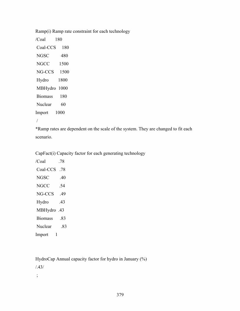
379

Ramp(i) Ramp rate constraint for each technology

/Coal 180

Coal-CCS 180

NGSC 480

NGCC 1500

NG-CCS 1500

Hydro 1800

MBHydro 1000

Biomass 180

Nuclear 60

Import 1000

/

*Ramp rates are dependent on the scale of the system. They are changed to fit each

scenario.

CapFact(i) Capacity factor for each generating technology

/Coal .78

Coal-CCS .78

NGSC .40

NGCC .54

NG-CCS .49

Hydro .43

MBHydro .43

Biomass .83

Nuclear .83

Import 1

HydroCap Annual capacity factor for hydro in January (%)

/.43/

;

380

Variable

Gen(h,i) Generation per hour by electricity source

;

Positive variable

Gen

Storage

WindStore

UseStore

UseWind

Curtail

SolarStore

UseSolar

SolarCurtail

DSMsave

DSMspend;

*Setting Upper (.up) and Lower (.lo) Bounds and Initial values (.l)

Gen.up(h,i) = GCAP(i) ;

Gen.lo(h,'hydro') = 20;

*The lower bound for hydro corresponds to the minimum streamflow, and resulting

electricity generation, that must be maintained at E.B. Campbell

Storage.l('1') = 0 ;

Storage.up(h) = Storecap * (744/400) ;

DSMsave.up(h) = 67;

DSMspend.up(h) = 67;

Variable

z total operating cost;

381

Equations

cost define objective function

MeetSupply(h) electricity generated will meet demand

Rampup(h,i) how quickly generation technologies can ramp up

Rampdown(h,i) how quickly generation technologies can ramp down

CapacityLimit(i) constrains generation technologies to operate within capacity factor

Store(h) specify how storage works

Windy(h) specify how wind power works

Sunny(h) specify how solar power works

DSM(h) allow peak shifting by 3 hours

;

*The equations are defined below.

*Ramping constraints limit the speed at which generation capacity can change

Rampup(h,i) .. Gen(h+1,i) - Gen(h,i) =l= Ramp(i);

Rampdown(h,i) .. Gen(h+1,i) - Gen(h,i) =g= -Ramp(i);

Meetsupply(h) .. d(h) - DSMsave(h) + DSMspend(h) =l= sum(i, (Gen(h,i) )) +

Usewind(h) + UseSolar(h) + .7*Usestore(h) ;

cost .. z =e= (sum(h,(sum(i,(VOM(i)+Fuel(i))*(Gen(h,i)))))) + (GasAdd*CapCost) ;

CapacityLimit .. (sum(h,Gen(h,i))) =l= CapFact(i)*744*GCAP(i) ;

Store(h) .. Storage(h+1) =e= Storage(h) + Windstore(h+1) + Solarstore(h+1) –

Usestore(h+1);

Windy(h) .. WindGen(h) =e= Windstore(h) + Usewind(h) + Curtail(h) ;

382

Sunny(h) .. SolarGen(h)=e= SolarStore(h) + UseSolar(h) + SolarCurtail(h);

DSM(h) .. DSMsave(h) =e= DSMspend(h+3);

Model WIRE /all/ ;

Option Reslim = 1000000 ;

Option Iterlim = 1000000 ;

Solve WIRE using nlp minimizing z ;

*Unload results to GDX file in order to then export them to Excel

execute_unload "results1013March2050BAU.gdx" Gen.L Windstore.l Usewind.l

Curtail.l Usestore.l UseSolar.l DSMsave;

383

Appendix 8A – Cost of Service Model

SaskPower has a cost of service model that they use to translate the cost of generating

and distributing electricity into the electricity rates paid by customers. This cost of

service model adheres to a few general principles:

1. Cross-subsidization is minimized. Cross-subsidization refers to charging more

for electricity to some electricity users in order to charge less, or subsidize, others.

SaskPower tries to avoid cross-subsidization in their current cost of service

model;

2. Large power customers pay for the transmission, but not for the distribution of

electricity. Transmission lines are the large, high-voltage lines that carry

electricity from power plants to major load centres. These lines will often serve

major power users like potash mines or oil refineries directly. Transmission lines

in Saskatchewan are typically 230 kilovolts (kV), 138 kV, 115 kV, or 110 kV.

Lower voltage lines (25 kV and 14.4 kV), linked to transmission lines at

substations, are used to provide electricity to commercial and residential

customers (SaskPower, 2011). These low-voltage distribution lines are the power

lines we see throughout towns and cities in the province. Figure 7A.1 shows a

transmission line with a smaller distribution line running beneath. Because large

power users do not use the distribution network, they do not pay the costs of

building and maintaining the network of low voltage lines;

3. Customer groups that use more power at peak times pay a premium for their

electricity. The electricity system must be sized large enough to meet peak

demand. As shown in Figure 6-5, electricity demand from large industrial power

customers is relatively stable. Electricity demand from residential and commercial

customers displays peaks in periods of high demand. These peaks require

additional generation capacity to be made available and, as a consequence,

residential and commercial customers pay more for their electricity.

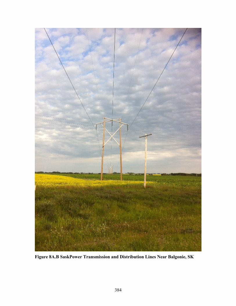
384

Figure 8A.B SaskPower Transmission and Distribution Lines Near Balgonie, SK

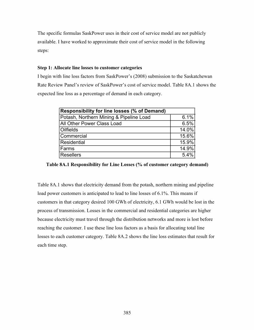
385

The specific formulas SaskPower uses in their cost of service model are not publicly

available. I have worked to approximate their cost of service model in the following

steps:

Step 1: Allocate line losses to customer categories

I begin with line loss factors from SaskPower’s (2008) submission to the Saskatchewan

Rate Review Panel’s review of SaskPower’s cost of service model. Table 8A.1 shows the

expected line loss as a percentage of demand in each category.

Table 8A.1 Responsibility for Line Losses (% of customer category demand)

Table 8A.1 shows that electricity demand from the potash, northern mining and pipeline

load power customers is anticipated to lead to line losses of 6.1%. This means if

customers in that category desired 100 GWh of electricity, 6.1 GWh would be lost in the

process of transmission. Losses in the commercial and residential categories are higher

because electricity must travel through the distribution networks and more is lost before

reaching the customer. I use these line loss factors as a basis for allocating total line

losses to each customer category. Table 8A.2 shows the line loss estimates that result for

each time step.

Responsibility for line losses (% of Demand)Potash, Northern Mining & Pipeline Load 6.1%All Other Power Class Load 6.5%Oilfields 14.0%Commercial 15.6%Residential 15.9%Farms 14.9%Resellers 5.4%

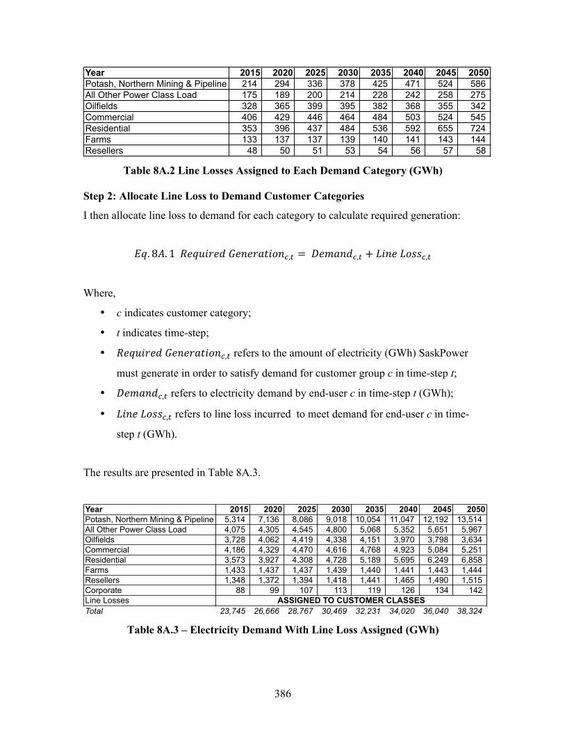
386

Table 8A.2 Line Losses Assigned to Each Demand Category (GWh)

Step 2: Allocate Line Loss to Demand Customer Categories

I then allocate line loss to demand for each category to calculate required generation:

𝐸𝑞. 8𝐴. 1 𝑅𝑒𝑞𝑢𝑖𝑟𝑒𝑑 𝐺𝑒𝑛𝑒𝑟𝑎𝑡𝑖𝑜𝑛!,! = 𝐷𝑒𝑚𝑎𝑛𝑑!,! + 𝐿𝑖𝑛𝑒 𝐿𝑜𝑠𝑠!,!

Where,

• c indicates customer category;

• t indicates time-step;

• 𝑅𝑒𝑞𝑢𝑖𝑟𝑒𝑑 𝐺𝑒𝑛𝑒𝑟𝑎𝑡𝑖𝑜𝑛!,! refers to the amount of electricity (GWh) SaskPower

must generate in order to satisfy demand for customer group c in time-step t;

• 𝐷𝑒𝑚𝑎𝑛𝑑!,! refers to electricity demand by end-user c in time-step t (GWh);

• 𝐿𝑖𝑛𝑒 𝐿𝑜𝑠𝑠!,! refers to line loss incurred to meet demand for end-user c in time-

step t (GWh).

The results are presented in Table 8A.3.

Table 8A.3 – Electricity Demand With Line Loss Assigned (GWh)

Year 2015 2020 2025 2030 2035 2040 2045 2050Potash, Northern Mining & Pipeline 214 294 336 378 425 471 524 586 All Other Power Class Load 175 189 200 214 228 242 258 275 Oilfields 328 365 399 395 382 368 355 342 Commercial 406 429 446 464 484 503 524 545 Residential 353 396 437 484 536 592 655 724 Farms 133 137 137 139 140 141 143 144 Resellers 48 50 51 53 54 56 57 58

Year 2015 2020 2025 2030 2035 2040 2045 2050Potash, Northern Mining & Pipeline Load5,314 7,136 8,086 9,018 10,054 11,047 12,192 13,514 All Other Power Class Load 4,075 4,305 4,545 4,800 5,068 5,352 5,651 5,967 Oilfields 3,728 4,062 4,419 4,338 4,151 3,970 3,798 3,634 Commercial 4,186 4,329 4,470 4,616 4,768 4,923 5,084 5,251 Residential 3,573 3,927 4,308 4,728 5,189 5,695 6,249 6,858 Farms 1,433 1,437 1,437 1,439 1,440 1,441 1,443 1,444 Resellers 1,348 1,372 1,394 1,418 1,441 1,465 1,490 1,515 Corporate 88 99 107 113 119 126 134 142 Line LossesTotal 23,745 26,666 28,767 30,469 32,231 34,020 36,040 38,324

ASSIGNED TO CUSTOMER CLASSES

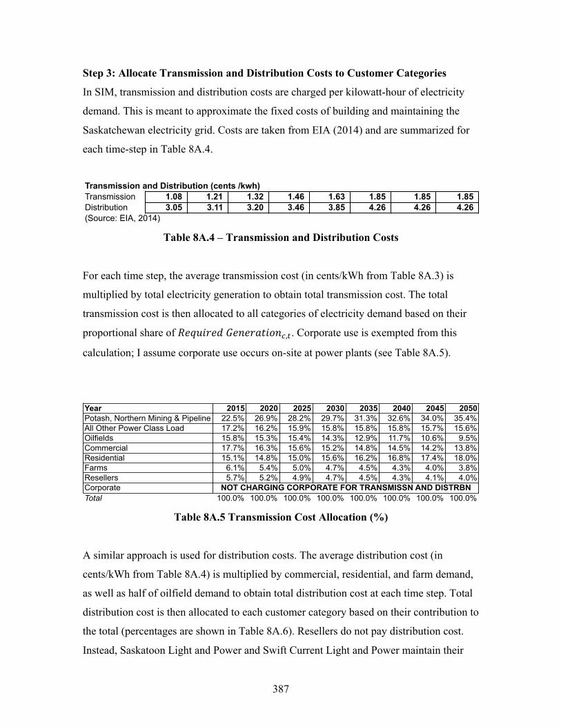
387

Step 3: Allocate Transmission and Distribution Costs to Customer Categories

In SIM, transmission and distribution costs are charged per kilowatt-hour of electricity

demand. This is meant to approximate the fixed costs of building and maintaining the

Saskatchewan electricity grid. Costs are taken from EIA (2014) and are summarized for

each time-step in Table 8A.4.

Table 8A.4 – Transmission and Distribution Costs

For each time step, the average transmission cost (in cents/kWh from Table 8A.3) is

multiplied by total electricity generation to obtain total transmission cost. The total

transmission cost is then allocated to all categories of electricity demand based on their

proportional share of 𝑅𝑒𝑞𝑢𝑖𝑟𝑒𝑑 𝐺𝑒𝑛𝑒𝑟𝑎𝑡𝑖𝑜𝑛!,!. Corporate use is exempted from this

calculation; I assume corporate use occurs on-site at power plants (see Table 8A.5).

Table 8A.5 Transmission Cost Allocation (%)

A similar approach is used for distribution costs. The average distribution cost (in

cents/kWh from Table 8A.4) is multiplied by commercial, residential, and farm demand,

as well as half of oilfield demand to obtain total distribution cost at each time step. Total

distribution cost is then allocated to each customer category based on their contribution to

the total (percentages are shown in Table 8A.6). Resellers do not pay distribution cost.

Instead, Saskatoon Light and Power and Swift Current Light and Power maintain their

Transmission and Distribution (cents /kwh)Transmission 1.08 1.21 1.32 1.46 1.63 1.85 1.85 1.85 Distribution 3.05 3.11 3.20 3.46 3.85 4.26 4.26 4.26 (Source: EIA, 2014)

Year 2015 2020 2025 2030 2035 2040 2045 2050Potash, Northern Mining & Pipeline Load22.5% 26.9% 28.2% 29.7% 31.3% 32.6% 34.0% 35.4%All Other Power Class Load 17.2% 16.2% 15.9% 15.8% 15.8% 15.8% 15.7% 15.6%Oilfields 15.8% 15.3% 15.4% 14.3% 12.9% 11.7% 10.6% 9.5%Commercial 17.7% 16.3% 15.6% 15.2% 14.8% 14.5% 14.2% 13.8%Residential 15.1% 14.8% 15.0% 15.6% 16.2% 16.8% 17.4% 18.0%Farms 6.1% 5.4% 5.0% 4.7% 4.5% 4.3% 4.0% 3.8%Resellers 5.7% 5.2% 4.9% 4.7% 4.5% 4.3% 4.1% 4.0%CorporateTotal 100.0% 100.0% 100.0% 100.0% 100.0% 100.0% 100.0% 100.0%

NOT CHARGING CORPORATE FOR TRANSMISSN AND DISTRBN

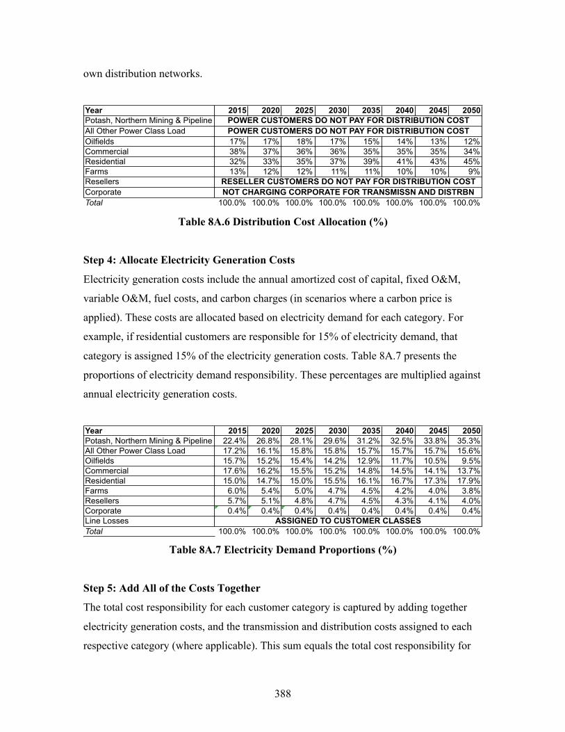
388

own distribution networks.

Table 8A.6 Distribution Cost Allocation (%)

Step 4: Allocate Electricity Generation Costs

Electricity generation costs include the annual amortized cost of capital, fixed O&M,

variable O&M, fuel costs, and carbon charges (in scenarios where a carbon price is

applied). These costs are allocated based on electricity demand for each category. For

example, if residential customers are responsible for 15% of electricity demand, that

category is assigned 15% of the electricity generation costs. Table 8A.7 presents the

proportions of electricity demand responsibility. These percentages are multiplied against

annual electricity generation costs.

Table 8A.7 Electricity Demand Proportions (%)

Step 5: Add All of the Costs Together

The total cost responsibility for each customer category is captured by adding together

electricity generation costs, and the transmission and distribution costs assigned to each

respective category (where applicable). This sum equals the total cost responsibility for

Year 2015 2020 2025 2030 2035 2040 2045 2050Potash, Northern Mining & Pipeline LoadAll Other Power Class Load Oilfields 17% 17% 18% 17% 15% 14% 13% 12%Commercial 38% 37% 36% 36% 35% 35% 35% 34%Residential 32% 33% 35% 37% 39% 41% 43% 45%Farms 13% 12% 12% 11% 11% 10% 10% 9%ResellersCorporateTotal 100.0% 100.0% 100.0% 100.0% 100.0% 100.0% 100.0% 100.0%

RESELLER CUSTOMERS DO NOT PAY FOR DISTRIBUTION COSTNOT CHARGING CORPORATE FOR TRANSMISSN AND DISTRBN

POWER CUSTOMERS DO NOT PAY FOR DISTRIBUTION COSTPOWER CUSTOMERS DO NOT PAY FOR DISTRIBUTION COST

Year 2015 2020 2025 2030 2035 2040 2045 2050Potash, Northern Mining & Pipeline Load22.4% 26.8% 28.1% 29.6% 31.2% 32.5% 33.8% 35.3%All Other Power Class Load 17.2% 16.1% 15.8% 15.8% 15.7% 15.7% 15.7% 15.6%Oilfields 15.7% 15.2% 15.4% 14.2% 12.9% 11.7% 10.5% 9.5%Commercial 17.6% 16.2% 15.5% 15.2% 14.8% 14.5% 14.1% 13.7%Residential 15.0% 14.7% 15.0% 15.5% 16.1% 16.7% 17.3% 17.9%Farms 6.0% 5.4% 5.0% 4.7% 4.5% 4.2% 4.0% 3.8%Resellers 5.7% 5.1% 4.8% 4.7% 4.5% 4.3% 4.1% 4.0%Corporate 0.4% 0.4% 0.4% 0.4% 0.4% 0.4% 0.4% 0.4%Line LossesTotal 100.0% 100.0% 100.0% 100.0% 100.0% 100.0% 100.0% 100.0%

ASSIGNED TO CUSTOMER CLASSES

389

each category.

Step 6: Calculate Net Demand for Electricity

To establish the net demand for electricity we need to subtract electricity saved through

demand side management (DSM) from total demand. DSM savings are allocated to each

customer category based on the assumptions made in Chapter 6 regarding DSM potential.

To recap,

Industrial DSM savings are allocated based on their contribution to the total of the

following:

• Potash, northern mining, and pipeline load +

• Oilfields +

• 75% of Other power users.

Commercial DSM savings are allocated based on their contribution to the total of the

following:

• Commercial +

• 50% of Reseller +

• 25% of Other power users.

Residential DSM savings are allocated based on their contribution to the total of the

following:

• Residential +

• Farms +

• 50% of Reseller.

Tables 8A.8 to 8A.10 show the proportions of DSM savings assigned to each customer

category. The proportions vary by year depending on relative electricity demand from

each customer category.

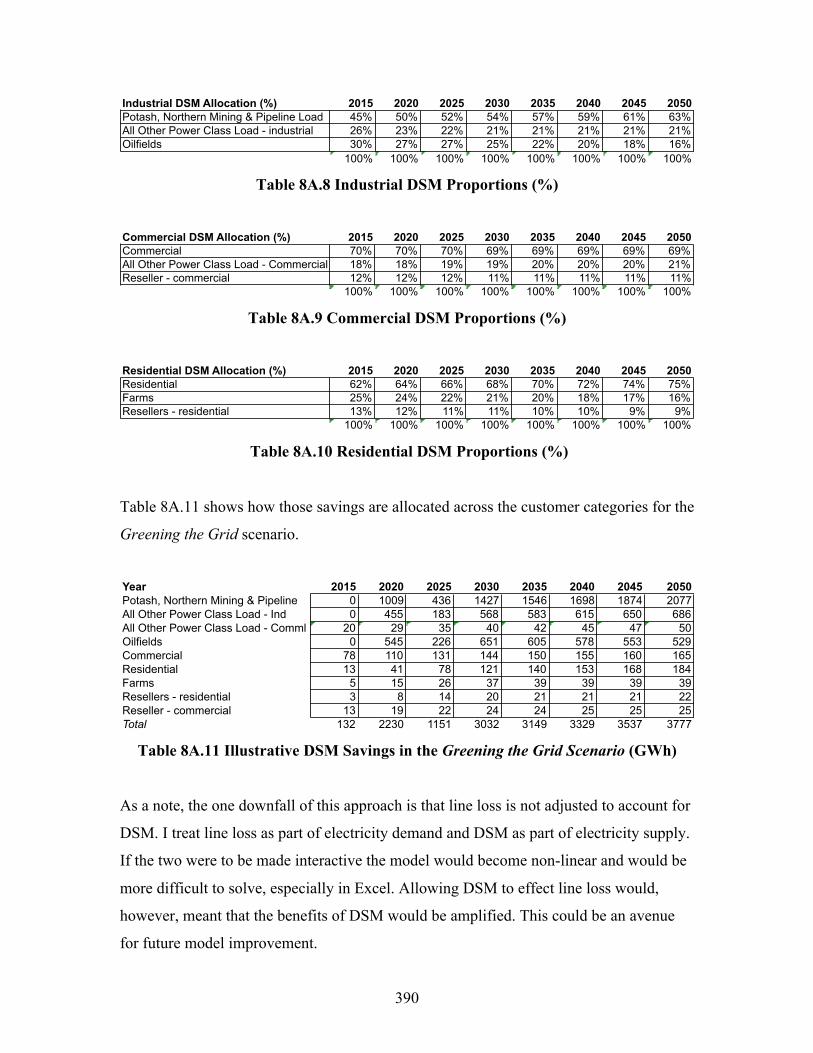
390

Table 8A.8 Industrial DSM Proportions (%)

Table 8A.9 Commercial DSM Proportions (%)

Table 8A.10 Residential DSM Proportions (%)

Table 8A.11 shows how those savings are allocated across the customer categories for the

Greening the Grid scenario.

Table 8A.11 Illustrative DSM Savings in the Greening the Grid Scenario (GWh)

As a note, the one downfall of this approach is that line loss is not adjusted to account for

DSM. I treat line loss as part of electricity demand and DSM as part of electricity supply.

If the two were to be made interactive the model would become non-linear and would be

more difficult to solve, especially in Excel. Allowing DSM to effect line loss would,

however, meant that the benefits of DSM would be amplified. This could be an avenue

for future model improvement.

Industrial DSM Allocation (%) 2015 2020 2025 2030 2035 2040 2045 2050Potash, Northern Mining & Pipeline Load 45% 50% 52% 54% 57% 59% 61% 63%All Other Power Class Load - industrial 26% 23% 22% 21% 21% 21% 21% 21%Oilfields 30% 27% 27% 25% 22% 20% 18% 16%

100% 100% 100% 100% 100% 100% 100% 100%

Commercial DSM Allocation (%) 2015 2020 2025 2030 2035 2040 2045 2050Commercial 70% 70% 70% 69% 69% 69% 69% 69%All Other Power Class Load - Commercial 18% 18% 19% 19% 20% 20% 20% 21%Reseller - commercial 12% 12% 12% 11% 11% 11% 11% 11%

100% 100% 100% 100% 100% 100% 100% 100%

Residential DSM Allocation (%) 2015 2020 2025 2030 2035 2040 2045 2050Residential 62% 64% 66% 68% 70% 72% 74% 75%Farms 25% 24% 22% 21% 20% 18% 17% 16%Resellers - residential 13% 12% 11% 11% 10% 10% 9% 9%

100% 100% 100% 100% 100% 100% 100% 100%

Year 2015 2020 2025 2030 2035 2040 2045 2050Potash, Northern Mining & Pipeline 0 1009 436 1427 1546 1698 1874 2077All Other Power Class Load - Ind 0 455 183 568 583 615 650 686All Other Power Class Load - Comml 20 29 35 40 42 45 47 50Oilfields 0 545 226 651 605 578 553 529Commercial 78 110 131 144 150 155 160 165Residential 13 41 78 121 140 153 168 184Farms 5 15 26 37 39 39 39 39Resellers - residential 3 8 14 20 21 21 21 22Reseller - commercial 13 19 22 24 24 25 25 25Total 132 2230 1151 3032 3149 3329 3537 3777

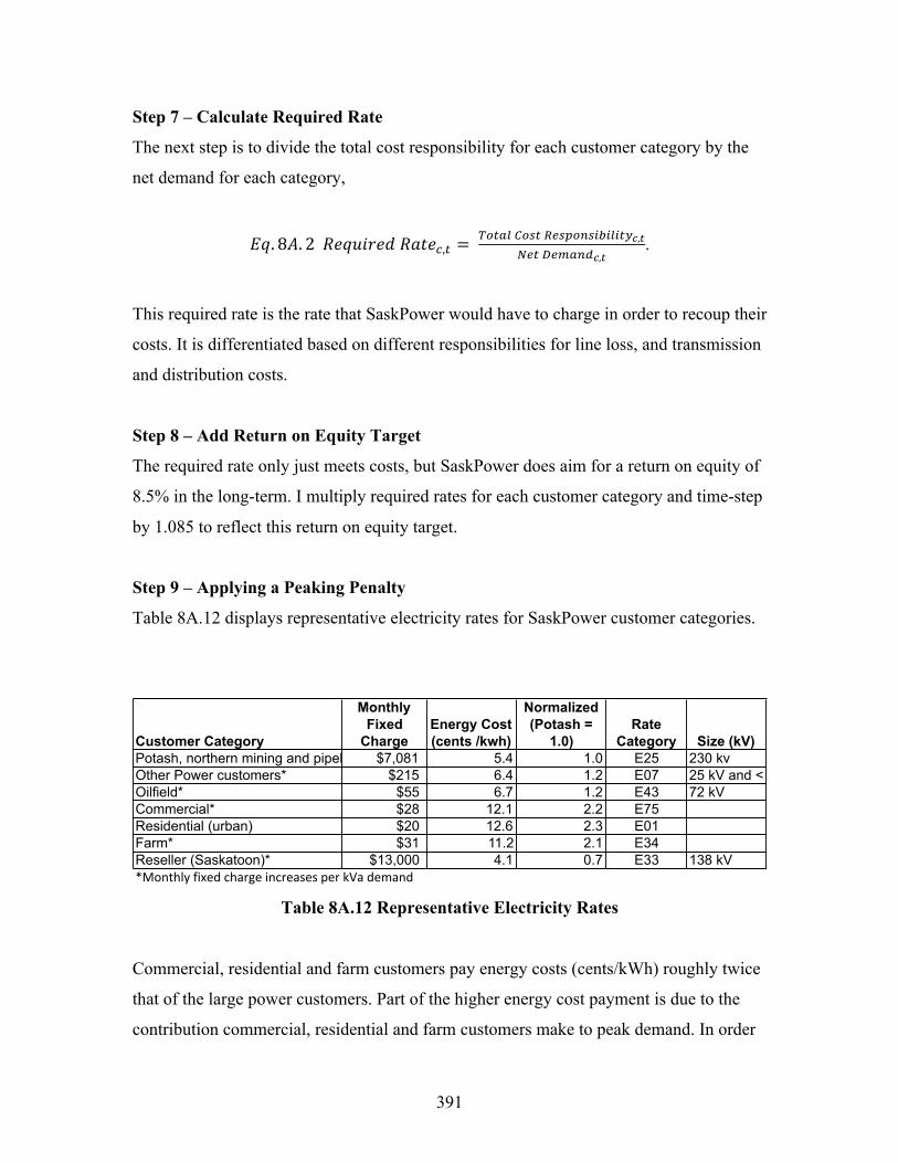
391

Step 7 – Calculate Required Rate

The next step is to divide the total cost responsibility for each customer category by the

net demand for each category,

𝐸𝑞. 8𝐴. 2 𝑅𝑒𝑞𝑢𝑖𝑟𝑒𝑑 𝑅𝑎𝑡𝑒!,! = !"#$% !"#! !"#$%&#'(')'*+!,!!"# !"#$%&!,!

.

This required rate is the rate that SaskPower would have to charge in order to recoup their

costs. It is differentiated based on different responsibilities for line loss, and transmission

and distribution costs.

Step 8 – Add Return on Equity Target

The required rate only just meets costs, but SaskPower does aim for a return on equity of

8.5% in the long-term. I multiply required rates for each customer category and time-step

by 1.085 to reflect this return on equity target.

Step 9 – Applying a Peaking Penalty

Table 8A.12 displays representative electricity rates for SaskPower customer categories.

Table 8A.12 Representative Electricity Rates

Commercial, residential and farm customers pay energy costs (cents/kWh) roughly twice

that of the large power customers. Part of the higher energy cost payment is due to the

contribution commercial, residential and farm customers make to peak demand. In order

Customer Category

Monthly Fixed

ChargeEnergy Cost (cents /kwh)

Normalized (Potash =

1.0)Rate

Category Size (kV)Potash, northern mining and pipeline* $7,081 5.4 1.0 E25 230 kvOther Power customers* $215 6.4 1.2 E07 25 kV and <Oilfield* $55 6.7 1.2 E43 72 kVCommercial* $28 12.1 2.2 E75Residential (urban) $20 12.6 2.3 E01Farm* $31 11.2 2.1 E34Reseller (Saskatoon)* $13,000 4.1 0.7 E33 138 kV*MonthlyfixedchargeincreasesperkVademand

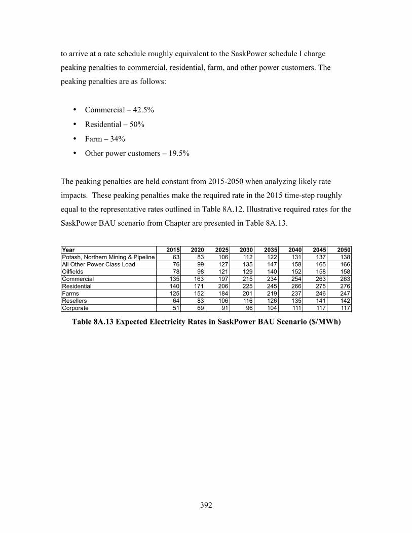
392

to arrive at a rate schedule roughly equivalent to the SaskPower schedule I charge

peaking penalties to commercial, residential, farm, and other power customers. The

peaking penalties are as follows:

• Commercial – 42.5%

• Residential – 50%

• Farm – 34%

• Other power customers – 19.5%

The peaking penalties are held constant from 2015-2050 when analyzing likely rate

impacts. These peaking penalties make the required rate in the 2015 time-step roughly

equal to the representative rates outlined in Table 8A.12. Illustrative required rates for the

SaskPower BAU scenario from Chapter are presented in Table 8A.13.

Table 8A.13 Expected Electricity Rates in SaskPower BAU Scenario ($/MWh)

Year 2015 2020 2025 2030 2035 2040 2045 2050Potash, Northern Mining & Pipeline Load 63 83 106 112 122 131 137 138All Other Power Class Load 76 99 127 135 147 158 165 166Oilfields 78 98 121 129 140 152 158 158Commercial 135 163 197 215 234 254 263 263Residential 140 171 206 225 245 266 275 276Farms 125 152 184 201 219 237 246 247Resellers 64 83 106 116 126 135 141 142Corporate 51 69 91 96 104 111 117 117

393

Appendix 9A – Post-Workshop Survey

Opportunities and Barriers for Renewable Energy and Energy Conservation in Saskatchewan

Post-Workshop Survey

Thank-you for participating in the energy-modelling workshop focused on ‘Opportunities and Barriers for Renewable Energy and Energy Conservation in Saskatchewan.’ Please answer the 6 questions below to the best of your ability. This workbook should take approximately 10 minutes to complete. For comparative purposes with our earlier survey responses please indicate your name: Name: ____________________________ Note that your response will not be attributed to you personally. Thank-you, Brett Dolter PhD researcher York University

394

Question 1 - Renewable electricity generation technologies include: biomass, hydroelectric, solar photovoltaic, solar thermal, and wind generation. In 2014, renewables supplied 23% of Saskatchewan's electricity demand with hydroelectricity providing 20%, wind providing 3%, and small contributions from solar photovoltaics and biomass. What is the maximum proportion of Saskatchewan electricity that renewables can supply in the medium-term (i.e. by 2030-2035)? Insert Response Here (%): _________________________ Question 2 - What is the maximum proportion of Saskatchewan electricity that renewables can supply in the long-term (i.e. by 2045-2050)? Insert Response Here (%): _________________________ Question 3 – Has your response changed from the earlier survey? YES / NO / UNSURE If yes, why?

395

Question 4 – Have you learned anything new from this workshop? (Please circle one) YES / NO / UNSURE Please explain: Question 5 – Did you enjoy the experience of interacting with others in this workshop setting? YES / NO / NEUTRAL Comments:

396

Question 6 – Please indicate with a checkmark which of the following are VERY IMPORTANT barriers for increasing renewable energy and energy conservation in Saskatchewan: ___ Cost: The price of renewable electricity is too high. ___ Feed-in-Tariff: Saskatchewan does not pay preferred rates for renewable power. ___ Grid design: The Saskatchewan grid is not optimized for renewables. ___ Job loss: A focus on renewables will lead to lost jobs in the coal-power industry. ___ Intermittency: Renewables cannot provide reliable electricity. ___ Physical limits: Saskatchewan lacks adequate hydro, solar, wind resources. ___ Political will: Political leaders in Saskatchewan have not prioritized renewables. ___ Preference for coal: SaskPower has a preference for coal-fired generation. ___ Public ownership: A private market would increase renewables more quickly. ___ Social acceptance: People do not want to live near renewable energy generation. ___ Other: ___ Other: General Comments: Thank-you for your time and participation! I look forward to sharing the results of this project with you! Best wishes, Brett

397

Appendix 9B – Workshop Script

Workshop Outline Session I – Introduction & Context: 1:00 p.m. – 2:30 p.m. 1:00-1:30 – WELCOME, INTRODUCTIONS, GROUND RULES Points to Convey

• Thank-you | Grateful for time • Introduce myself | As many of you know, I’m Brett Dolter, I’m the PhD student

who invited you to this meeting. • Introduce Scott | I’m joined today by Scott Fulton our facilitator for the day. • Round Table | Before we get started I’d just like to do a round table so let’s go

around the room and please state your names and your affiliation if you’d like to state it

o ROUND TABLE • Great – we have a lot of expertise around the table. We’re going to have a great

session. • Big Picture | We are at a seminal moment in climate change policy.

o BRETT – spell out climate policy context § To achieve 2DS we need to stop the growth of GHGs and reduce

to near-zero by 2050; § It will take a heroic effort to achieve it. Some have likened the

task to a second ‘moon-shot’. § This time the goal is to transition away from fuels that release

GHGs to the atmosphere. § Renewable energy such as: hydroelectricity, wind, solar, and

biomass offer the potential to decarbonize the electricity grid. § In my research project I am seeking to understand the costs,

barriers, opportunities, and trade-offs involved in pursuing a renewable energy pathway to a low-GHG future.

• There Are Three Objectives for Today | 1. I’ve invited you here today to ground-truth the models I’ve created.

o You have been invited to this workshop because you have expertise on the Saskatchewan electricity system. Your participation will help to ensure that the results of this research are valid and useful for the Saskatchewan public, and, I hope, SaskPower.

o “Models are a way of disciplining our thinking.” I want to test the assumptions and the structure of the models I’ve created.

2. Use the Models to Create A Sunny skies, Winds of Change scenario for renewable energy in Saskatchewan. Goal is to leave here with clear

398

scenarios in our minds that provide a picture of a renewable energy future and a roadmap of how we would get to that future.

3. In the process Develop a shared understanding of the opportunities, costs, technical barriers, and environmental impacts of increasing the amount of renewable energy generated in the province o I’ve invited participants with diverse perspectives to the meeting so

that we can learn from each other. o We can take that learning back to our respective professional worlds.

• SCOTT | FACILITATION INTRODUCTION I’m Scott Fulton. I’m a teacher and educator. My role today is to host the conversation, and ensure that everyone has the chance to participate, and that we move through the agenda and stay on time so that we can all leave on time. o Do I have everyone’s permission to intervene to ensure everyone has the

opportunity to speak and to keep the conversation moving? o Also – there will likely be different perspectives on the table today. They are

all welcomed. We can disagree without being disagreeable. • BRETT | GROUND RULES FOR HOW INFORMATION IS USED

o Here are some ground rules: § To encourage people to speak freely I’d like us all to recognize that

what is said today is not to be interpreted as the official position of any of the organizations present.

§ Basically, what is said in the room stays in the room, or at least is not attributed to any individual or organization.

• Do I have agreement on that? o We’ll be recording the session using audio and visual equipment. This is a

way to take notes so the discussion can inform my dissertation. o I’ve asked everyone to sign a consent form to participate in the workshop. If

you haven’t signed one please do so now. There is a clause at the back that states I will not release footage or audio of any participant without following up to again ask for written consent.

o With that I’d like to encourage everyone to bring curiousity, a willingness to listen, and creativity to the tasks ahead.

• ICEBREAKER 1:30-2:00 – HISTORY AND CONTEXT

• BRETT | I want to walk you through some of the history of the Saskatchewan electricity system so we understand where we are today, how we got here, and some of the challenges for the future.

• PRESENTATION

399

A Walk Through History

• Saskatchewan’s electricity system began in municipalities. Towns and cities built power plants to provide street lighting to residents. These were run on a ‘moonlight basis’, which means they were only turned on at night when the moon was not expected to shine.

• When the potential for electricity to transform Saskatchewan society became evident there were calls for rational development of the system.

• The Saskatchewan Power Commission was created in 1929 to work to coordinate and consolidate the Saskatchewan electricity system.

• With a centralized electricity system the Saskatchewan Power Commission could exploit ‘Cheap, lignite coal’ in South-eastern Saskatchewan and hydroelectric potential along the Saskatchewan River system.

• The Depression crushed demand for electricity. Demand only began to grow again leading into World War II. But Wartime rationing kept the system from expanding.

• Rapid and exponential growth of the electricity system began in the late 1940s and 1950s.

• In 1949 the Saskatchewan Power Commission became the Crown Corporation we now call SaskPower.

• SaskPower’s immediate task was to bring electricity to rural Saskatchewan. In the 1952 election Tommy Douglas had promised to electrify 40,000 new farms. This was a huge challenge for SaskPower.

• [READ QUOTE] • Rural electrification was a success and Tommy Douglas called it his greatest

achievement as Premier (greater than introducing Medicare to Canada) • I think it is a useful historic lesson for two reasons:

o 1. It shows great change is possible o 2. It shows how political promises and government policy can influence

SaskPower’s business • SaskPower continued to promote load growth in the 1950s, hiring people like

Lillian McConnell to speak as “Penny Power” educating Saskatchewan citizens about the virtues of electricity.

• She appears to have been successful [Point to load growth graph] • In 1965 SaskPower’s first hydroelectric facility was commissioned: E.B.

Campbell. • This was good news for most of the province, but did have impacts on the people

of Cumberland House downstream from the dam. [QUOTE] • 1965 was also the year that Regina City Council agreed to let SaskPower sell and

distribute electricity in the city. • Regina was the last brick on the wall of creating a centralized electricity system in

Saskatchewan. • Centralization lowered costs and allowed power created by ‘cheap, lignite coal’

and hydroelectricity to be transmitted around the province.

400

• The 1960s were the golden age of power production in the province, and across North America: demand was increasing, revenues and profits were rising, all was well.

• The 1970s were a more difficult period. The energy price shocks of the early 1970s led to inflation, making large capital projects like power plants more expensive.

• It was at this time that Penny Powers became a Penny Pincher and SaskPower shifted its focus from load promotion to energy conservation. Energy conservation could allow large capital projects to be deferred.

• To combat inflation, interest rates were increased. They reached a peak in the early 1980s. This meant that financing charges skyrocketed creating difficulties throughout the 1980s. By 1989 SaskPower’s debt had reached $2 billion dollars.

• The Progressive Conservatives planned to sell SaskEnergy to help pay off the debt. Privatization was now a clear threat for SaskPower.

• The late 1980s were also a time of increasing environmental awareness. SaskPower was caught in the thick of this with the proposed Rafferty-Alameda dam.

• The dam was given a federal government green light without an environmental assessment. The Canadian Wildlife Federation took the federal government to court and asked them to enforce their own guidelines for environmental assessment. The Wildlife Federation won their case, even though construction had started on the dam. Rafferty-Alameda now stands as a historic precedent in environmental law.

• It was in the 1990s that climate change concerns began to gain prominence. SaskPower recognized they would need to reduce their emissions in the future. By the late 1990s SaskPower began to diversify their operations, partnering to build a cogeneration plant at Lloydminster. The Corey Potash mine soon followed.

• The first wind projects: SunBridge and Cypress were completed in the early 2000s, and the 150 MW Centennial wind farm was put in place in time for the Centennial.

• Demand growth in recent years has been met with natural gas simple-cycle turbines, and combined cycle plants with some additions of wind to help reduce natural gas bills.

• There are challenges ahead. o The federal government has introduced regulations on coal-fired

electricity that require coal plants to be retired or retrofit to achieve a standard of 420 grams CO2e/kwh.

o Much of the SaskPower fleet is aging and is scheduled to retired in the next 15 years.

o Demand is still growing. • So now in this workshop we’ll explore opportunities for renewable energy and

energy conservation to help meet those challenges. • INFORMATION IN:

1. Comments? Reactions? Anything Surprising? Anything missing? 2. If there is anything missing let me know and I’ll add it to the timeline

using a sticky note.

401

2:00-2:30 – INTRODUCE THE MODEL & EXAMINING THE ASSUMPTIONS

• BRETT | We’ve talked about the past, now we’re going to look towards the future. In order to do that we’re going to use modelling as a tool.

• MODELLING 101 o Some people in the room are better modellers than me. If you have

reflections please contribute. Here is a little modelling 101. o What is a model?

§ Partial representation of reality § We choose what to include, what to exclude

o What can a model do? § “Models are tools for disciplining our thinking”

o What can a model not do? § “All models are wrong. Some models are useful.”

• SASKATCHEWAN INVESTMENT MODEL o Today we’re focusing on a model to decide what generation technologies

to invest in in order to meet electricity demand by 2050. o In technical terms the model is a linear programming optimization

model. The goal is to minimize the cost of generating electricity in Saskatchewan subject to constraints:

§ Constraint 1 – electricity supply must meet demand § Constraint 2 – firm, dispatchable capacity must be available to

meet peak demand § Supply Constraints:

• biomass potential limited to 300 MW • in most runs wind limited to 20% of electricity generation • hydro limits and increasing costs

• WORKBOOK o A model is only as good as the assumptions that go into it. I want to

draw upon the expertise in the room to test the assumptions that have gone into this model.

o There are three important areas I’d like feedback on: § Costs: capital costs now and in the future, fuel costs § Demand forecast & conservation potential: how much will

demand grow into the future? What is possible for energy conservation?

§ Renewable energy potential: how much biomass, hydro, wind, solar is possible?

o We’re going to break into three groups. One group for each focus area. o Please take 5 minutes to work through the workbook on your own and

then you’ll have 10 minutes to discuss your thoughts as a group. o I’ll then ask for one person from each group to provide a 5-minute

report on the discussion. o I’m also going to keep these recorders running in the groups so that I

can go back and track the input I’ve received. o I’ll take this input and use it to improve the model.

402

BREAK 2:30 – 2:45

• SCENARIOS – 2:45 – 3:45 o Lisa White surveyed a group of experts in her research and they

recommended a renewable energy pathway. o I’d like to flesh out what this renewable scenario looks like. We’re going

to create three new groups – I’d like members of the first groups to spread themselves around, so that each new group has representatives from the former groups.

o Each group is going to build a scenario for a renewable energy future. § Select which technologies to build, their quantities

o Survey response notes: there are different perspectives on what is possible so each group can create two scenarios:

§ An ambitious ‘sunny skies’ or ‘winds of change’ scenario with a high penetration of renewable energy

§ A moderate scenario with some penetration of renewables o As individuals you may disagree about which is most likely or best, but

the question to ask is: § What would have to be true in order for this scenario to be

preferred? § For example, perhaps the ambitious scenario is only possible if

we achieve low-cost electricity storage. § Please track these caveats.

o I’ll move around to each group and input these scenarios into the model so we can test them for their performance in terms of cost, GHGs, and other environmental indicators. Points for low-cost, low-GHG scenarios.

o At the beginning of the session please select a person in your group to report back to the group. At the end I’ll ask a representative from each group to present the scenarios the group has created.

o MODEL on the screen: § Here are the areas for entry into the model

• Change demand growth rates • Change cost inputs • Plan investment path

§ Here are the ways to see what the model has created o SCOTT – [moving around the room, sitting in and listening, making

sure that everyone has a chance to be heard.]

• REPORT BACK – 3:45 – 4:15 o Let’s have a reporter from each group. Each reporter has 5 minutes to

present the scenario. We’ll have ten minutes of discussion at the end. o I’ll take these scenarios away and test them in the ‘Will It Run

Electricity Model’.

• OPPORTUNITIES AND BARRIERS 4:15 – 4:45

403

o [Start: SCOTT ensure everyone has a sticky-note pad and a sharpie] o RECAP:

§ We’ve talked about the assumptions going into the model § We’ve talked about scenarios for the future § Now let’s talk about how we could make them real.

o In the survey I asked what the barriers were to more renewable energy in the province. The barriers people identified as most important were: x,y,z. I’ve listed all of those barriers on the wall here.

o You’re going to use the sticky notes to add to the list of barriers and to also create a list of opportunities to overcome the barriers. For example, the Cowessess wind and storage project is showing how wind power might be made less variable.

o We can also talk about opportunities outside the discussion of barriers. The FNPA has created an opportunity to expand renewable energy in the province in partnership with First Nations. Renewable energy here is an opportunity for inclusion of First Nations in the Saskatchewan economy.

o Take 5 minutes and come up with as many barriers and opportunities as you can think of.

§ Barriers are XX colour § Opportunities to overcome barriers are XX colour § [Facilitators – grab and post, encouraging them, reading them].

o I see a few people here mentioned XX, did someone who put that up want to explain it?

o Organize into themes. Conversation by theme.

• THANK-YOU 4:45 – 5:00 o Thank-you so much for your time. There is a quick survey I’d like you to

fill out before you leave. o There are a tremendous number of great ideas put on the table today. o Here are some I’m going to take away:

§ NOTE THINGS I’VE HEARD o I’m going to use this input to improve the model. I’ll share the results

with you when I’ve incorporated your input. o I just want to thank-you for this fantastic session. I think everyone

deserves a round of applause. [start clapping] o [SCOTT and I will start handing out the surveys]

404

Appendix 9C – Modelling Workbook

Introduction This workbook is designed to provide: 1. Information on how the model was

created, and 2. An opportunity for you to contribute to

the model. The model you will interact with today is a linear programming optimization model built in Excel. The model is used to determine the least-cost means of producing electricity in Saskatchewan. The model is shaped by constraints, including the constraint that the supply of electricity must equal demand.

405

The model solves by selecting investments in five-year planning periods to 2050.

406

1.0 Costs Costs are key inputs to the economic model. Generation technologies differ with respect to the following costs: • Capital cost: cost of building new

generation facilities measured in $CDN per kilowatt ($/kw)

• Fixed Operations & Maintenance (FOM) cost: annual fixed cost of operating generation facilities measured in $CDN per kilowatt per year ($/kw/yr)

• Variable Operations & Maintenance

(VOM) cost: cost of operating facilities and repairing wear-and-tear based on electricity output, measured in $CDN per Megawatt-hour ($/MWh)

• Fuel use and efficiency: thermal

generation uses coal or natural gas.

407

1.1 Capital Costs Cost data was taken largely from the U.S. Energy Information Agency (EIA). The EIA (2015) provides data on current and expected costs of electricity generation technologies in 2040. The EIA (2015) costs were compared to Saskatchewan and Canadian published reports of the costs of recent Saskatchewan and Canadian projects. A Saskatchewan multiplier was calculated to reflect differences between EIA costs and Saskatchewan achieved costs. In this model, costs change over time according to a pre-set rate. I call this the cost improvement rate. Explore the implications of changing cost parameters in the worksheet: ‘1.0 Cost Tables.’ Record revisions in Table 1b.

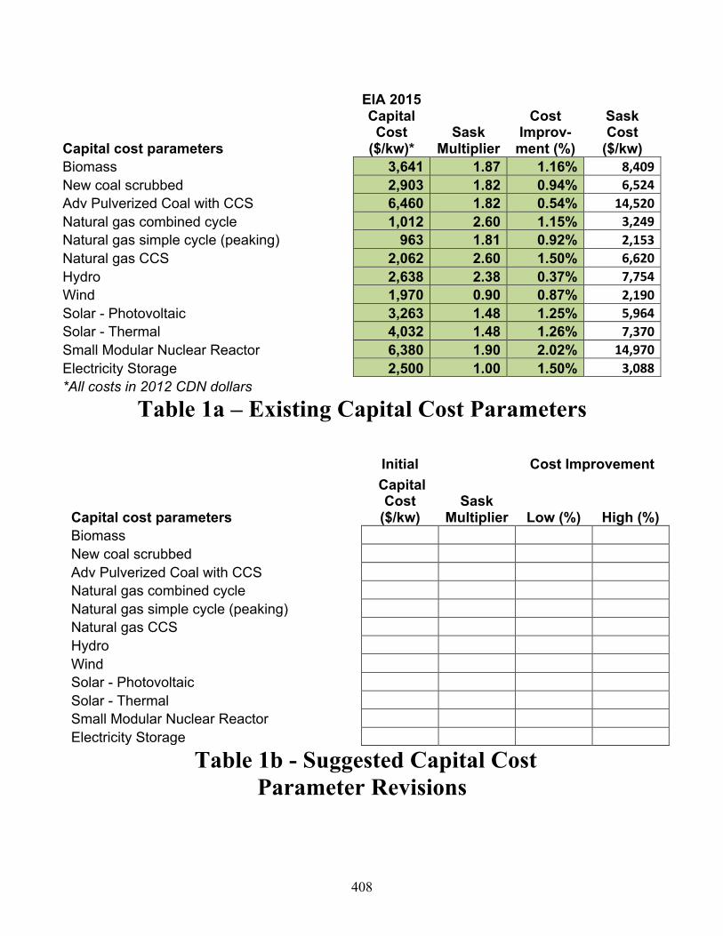
408

Capital cost parameters

EIA 2015 Capital Cost

($/kw)* Sask

Multiplier

Cost Improv-ment (%)

Sask Cost

($/kw) Biomass 3,641 1.87 1.16% 8,409New coal scrubbed 2,903 1.82 0.94% 6,524Adv Pulverized Coal with CCS 6,460 1.82 0.54% 14,520Natural gas combined cycle 1,012 2.60 1.15% 3,249Natural gas simple cycle (peaking) 963 1.81 0.92% 2,153Natural gas CCS 2,062 2.60 1.50% 6,620Hydro 2,638 2.38 0.37% 7,754Wind 1,970 0.90 0.87% 2,190Solar - Photovoltaic 3,263 1.48 1.25% 5,964Solar - Thermal 4,032 1.48 1.26% 7,370Small Modular Nuclear Reactor 6,380 1.90 2.02% 14,970Electricity Storage 2,500 1.00 1.50% 3,088*All costs in 2012 CDN dollars

Table 1a – Existing Capital Cost Parameters

Initial

Cost Improvement

Capital cost parameters

Capital Cost

($/kw) Sask

Multiplier Low (%) High (%) Biomass New coal scrubbed Adv Pulverized Coal with CCS Natural gas combined cycle Natural gas simple cycle (peaking) Natural gas CCS Hydro Wind Solar - Photovoltaic Solar - Thermal Small Modular Nuclear Reactor Electricity Storage

Table 1b - Suggested Capital Cost Parameter Revisions

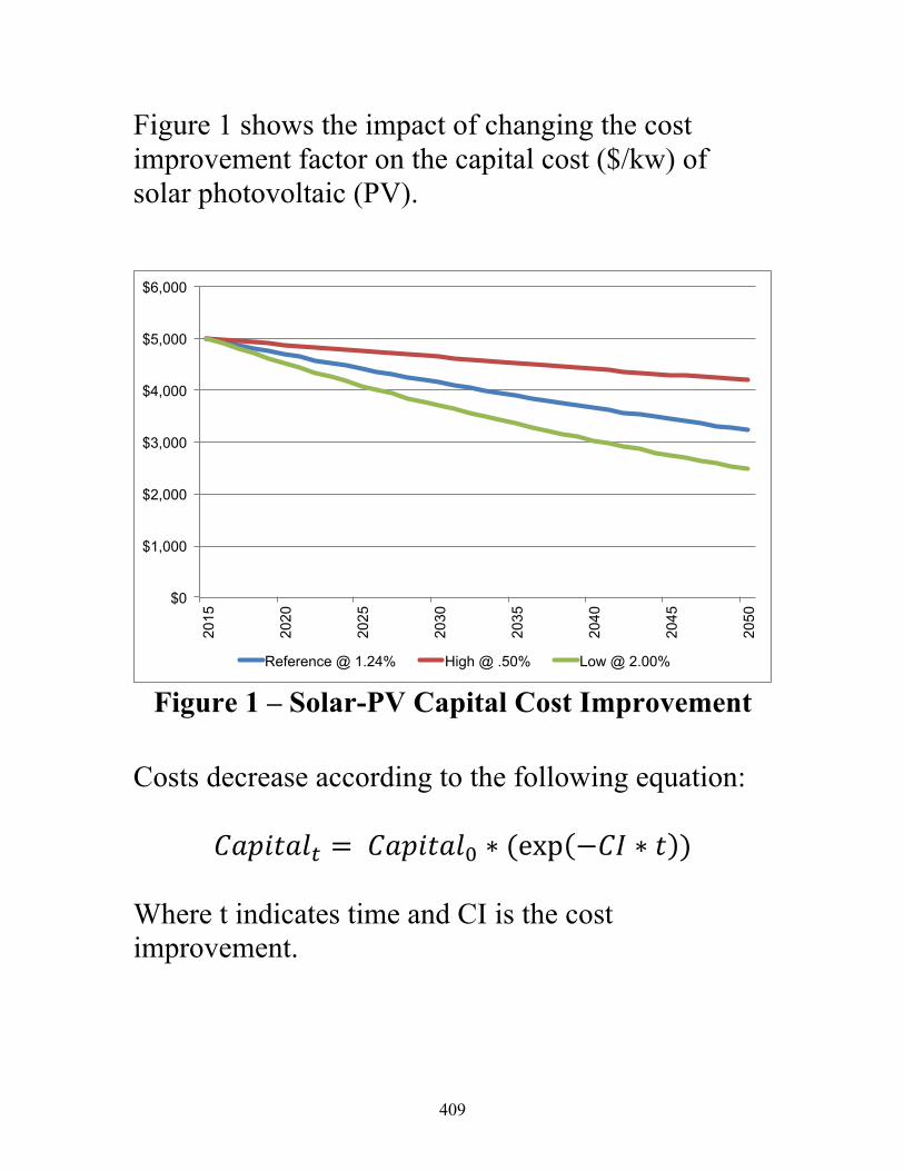
409

Figure 1 shows the impact of changing the cost improvement factor on the capital cost ($/kw) of solar photovoltaic (PV).

Figure 1 – Solar-PV Capital Cost Improvement

Costs decrease according to the following equation:

𝐶𝑎𝑝𝑖𝑡𝑎𝑙! = 𝐶𝑎𝑝𝑖𝑡𝑎𝑙! ∗ (exp −𝐶𝐼 ∗ 𝑡 ) Where t indicates time and CI is the cost improvement.

$0

$1,000

$2,000

$3,000

$4,000

$5,000

$6,000

2015

2020

2025

2030

2035

2040

2045

2050

Reference @ 1.24% High @ .50% Low @ 2.00%

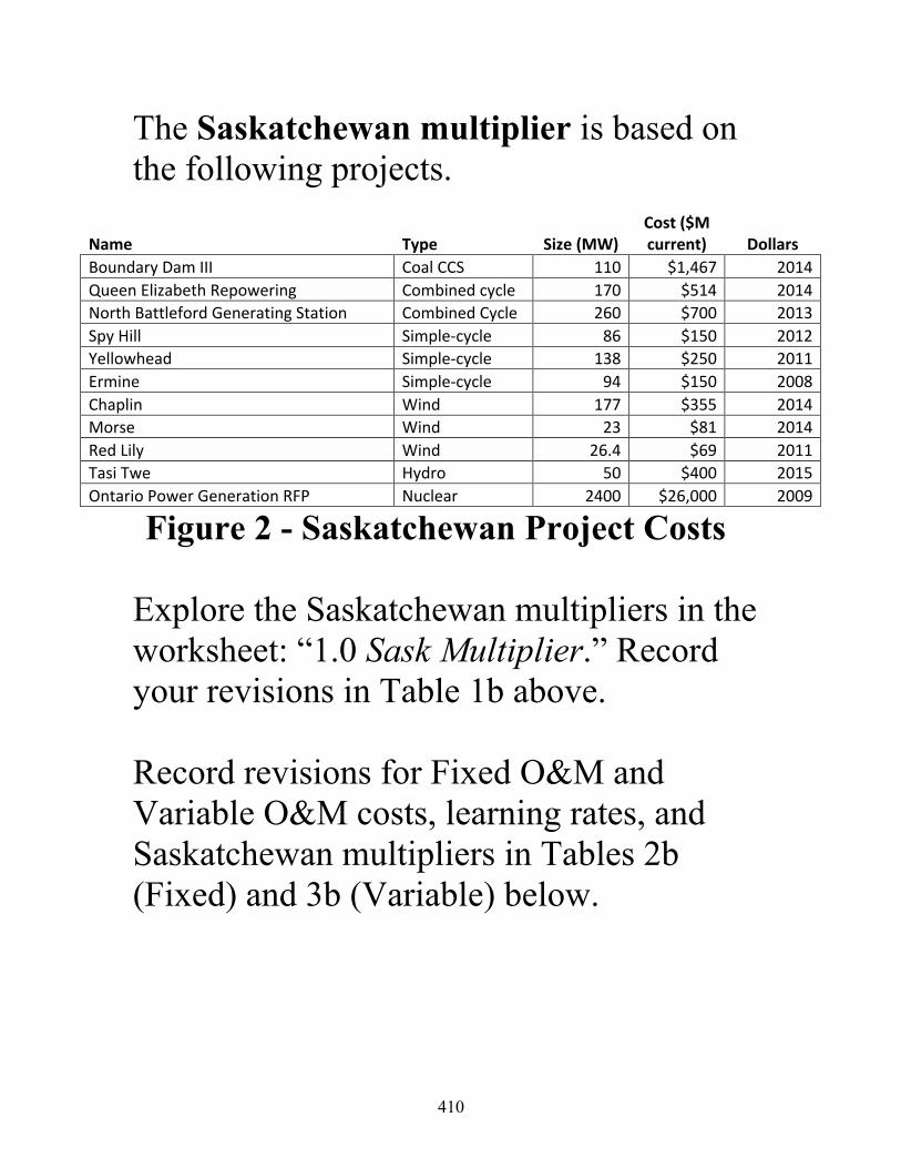
410

The Saskatchewan multiplier is based on the following projects.

Name Type Size(MW)Cost($Mcurrent) Dollars

BoundaryDamIII CoalCCS 110 $1,467 2014QueenElizabethRepowering Combinedcycle 170 $514 2014NorthBattlefordGeneratingStation CombinedCycle 260 $700 2013SpyHill Simple-cycle 86 $150 2012Yellowhead Simple-cycle 138 $250 2011Ermine Simple-cycle 94 $150 2008Chaplin Wind 177 $355 2014Morse Wind 23 $81 2014RedLily Wind 26.4 $69 2011TasiTwe Hydro 50 $400 2015OntarioPowerGenerationRFP Nuclear 2400 $26,000 2009

Figure 2 - Saskatchewan Project Costs

Explore the Saskatchewan multipliers in the worksheet: “1.0 Sask Multiplier.” Record your revisions in Table 1b above. Record revisions for Fixed O&M and Variable O&M costs, learning rates, and Saskatchewan multipliers in Tables 2b (Fixed) and 3b (Variable) below.

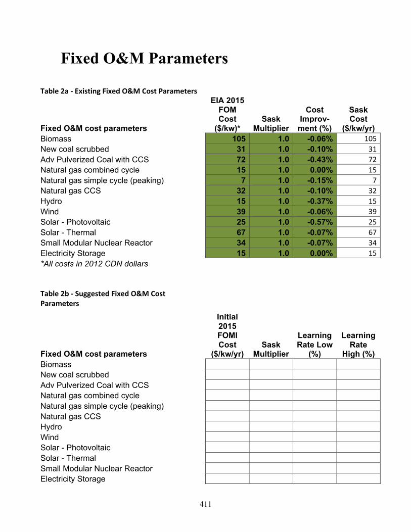
411

Fixed O&M Parameters

Table2a-ExistingFixedO&MCostParameters

Fixed O&M cost parameters

EIA 2015 FOM Cost

($/kw)* Sask

Multiplier

Cost Improv-ment (%)

Sask Cost

($/kw/yr) Biomass 105 1.0 -0.06% 105New coal scrubbed 31 1.0 -0.10% 31Adv Pulverized Coal with CCS 72 1.0 -0.43% 72Natural gas combined cycle 15 1.0 0.00% 15Natural gas simple cycle (peaking) 7 1.0 -0.15% 7Natural gas CCS 32 1.0 -0.10% 32Hydro 15 1.0 -0.37% 15Wind 39 1.0 -0.06% 39Solar - Photovoltaic 25 1.0 -0.57% 25Solar - Thermal 67 1.0 -0.07% 67Small Modular Nuclear Reactor 34 1.0 -0.07% 34Electricity Storage 15 1.0 0.00% 15*All costs in 2012 CDN dollars

Table2b-SuggestedFixedO&MCostParameters

Fixed O&M cost parameters

Initial 2015 FOMl Cost

($/kw/yr) Sask

Multiplier

Learning Rate Low

(%)

Learning Rate

High (%) Biomass New coal scrubbed Adv Pulverized Coal with CCS Natural gas combined cycle Natural gas simple cycle (peaking) Natural gas CCS Hydro Wind Solar - Photovoltaic Solar - Thermal Small Modular Nuclear Reactor Electricity Storage

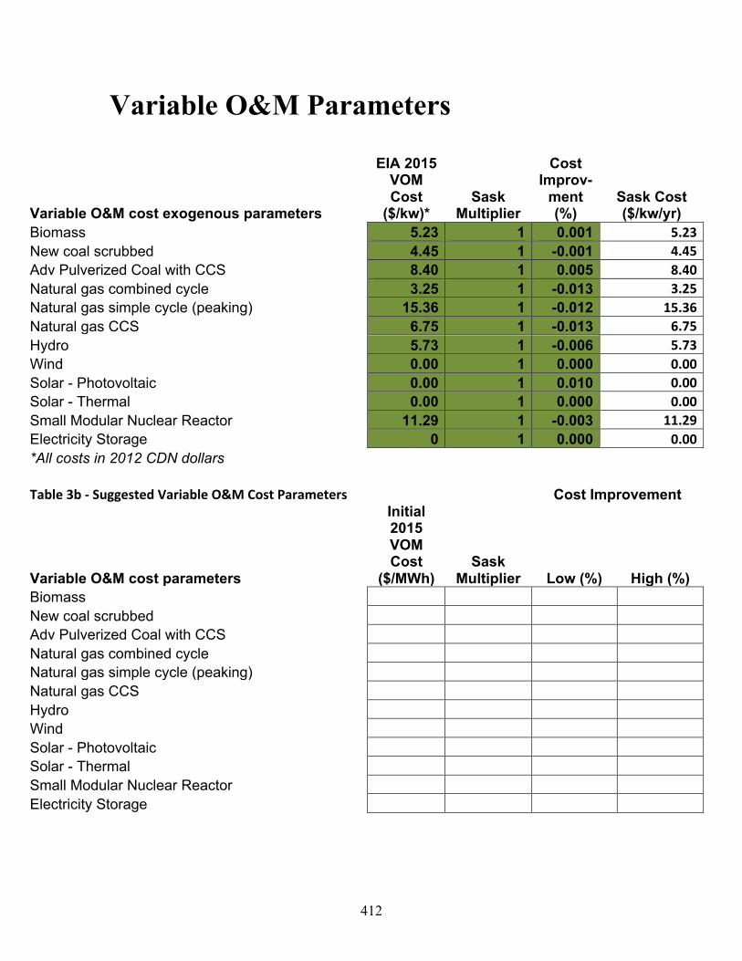
412

Variable O&M Parameters

Variable O&M cost exogenous parameters

EIA 2015 VOM Cost

($/kw)* Sask

Multiplier

Cost Improv-

ment (%)

Sask Cost ($/kw/yr)

Biomass 5.23 1 0.001 5.23New coal scrubbed 4.45 1 -0.001 4.45Adv Pulverized Coal with CCS 8.40 1 0.005 8.40Natural gas combined cycle 3.25 1 -0.013 3.25Natural gas simple cycle (peaking) 15.36 1 -0.012 15.36Natural gas CCS 6.75 1 -0.013 6.75Hydro 5.73 1 -0.006 5.73Wind 0.00 1 0.000 0.00Solar - Photovoltaic 0.00 1 0.010 0.00Solar - Thermal 0.00 1 0.000 0.00Small Modular Nuclear Reactor 11.29 1 -0.003 11.29Electricity Storage 0 1 0.000 0.00*All costs in 2012 CDN dollars

Table3b-SuggestedVariableO&MCostParameters

Cost Improvement

Variable O&M cost parameters

Initial 2015 VOM Cost

($/MWh) Sask

Multiplier Low (%) High (%) Biomass New coal scrubbed Adv Pulverized Coal with CCS Natural gas combined cycle Natural gas simple cycle (peaking) Natural gas CCS Hydro Wind Solar - Photovoltaic Solar - Thermal Small Modular Nuclear Reactor Electricity Storage

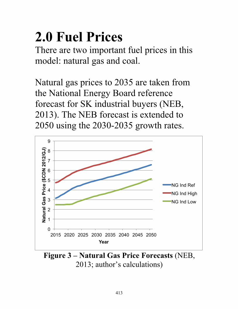
413

2.0 Fuel Prices There are two important fuel prices in this model: natural gas and coal. Natural gas prices to 2035 are taken from the National Energy Board reference forecast for SK industrial buyers (NEB, 2013). The NEB forecast is extended to 2050 using the 2030-2035 growth rates.

Figure 3 – Natural Gas Price Forecasts (NEB,

2013; author’s calculations)

0

1

2

3

4

5

6

7

8

9

2015 2020 2025 2030 2035 2040 2045 2050

Nat

ural

Gas

Pric

e ($

CD

N 2

012/

GJ)

Year

NG Ind Ref

NG Ind High

NG Ind Low

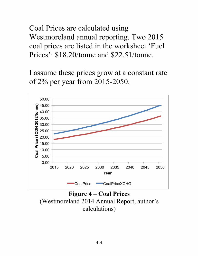
414

Coal Prices are calculated using Westmoreland annual reporting. Two 2015 coal prices are listed in the worksheet ‘Fuel Prices’: $18.20/tonne and $22.51/tonne. I assume these prices grow at a constant rate of 2% per year from 2015-2050.

Figure 4 – Coal Prices

(Westmoreland 2014 Annual Report, author’s calculations)

0.00 5.00

10.00 15.00 20.00 25.00 30.00 35.00 40.00 45.00 50.00

2015 2020 2025 2030 2035 2040 2045 2050

Coa

l Pric

e ($

CD

N 2

012/

tonn

e)

Year

CoalPrice CoalPriceXCHG

415

Please answer the following three questions: Q1. Which natural gas price forecast would you recommend using? o Reference o Low o High

Q2. What 2015 coal price would you recommend using? o $18.20 o $22.51 o Other ________________

Q3. What growth rate would you recommend using for coal price escalation? o 2%/yr o 1%/yr o Other ________________

416

3.0 Renewable Constraints To reflect Saskatchewan’s renewable energy potential and existing technical constraints and policy the following constraints have been introduced in the model:

1.Conventional hydroelectricity is limited to 1000 MW.

2.Biomass capacity is limited to 300 MW. 3.Wind generation is originally limited to

20% of total electricity generated in 2020. The wind generation constraint is allowed to grow 3% each 5-year investment period, reaching 38% by 2050.

4.Wind and solar generation does not contribute to firm capacity to meet peak demand.

5.Electricity storage must be paired with wind and solar to meet peak demand.

6.Electricity storage capacity cannot exceed 50% of wind & solar capacity.

417

7.Only 40% of electricity storage capacity contributes to meeting peak demand. This is based on some of the findings of the Cowessess wind project.

Please discuss these constraints and record suggested revisions below. When discussing each constraint it may be useful to ask: “What conditions would have to hold true in order for this constraint to be valid?” Discussion/Recommendations Biomass:

418

Hydroelectricity: Wind percentage: Electricity storage treatment:

419

4.0 Demand Growth I have created an electricity demand forecast to 2050 by extending the SaskPower 2014 Load Forecast to 2025 using annual growth rates. You can create your own forecast by adjusting the growth rates in the worksheet: ‘4.0 Electricity Demand.’ The existing forecast is summarized in Figure 5 on the following page.

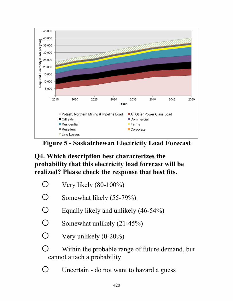
420

Figure 5 - Saskatchewan Electricity Load Forecast

Q4. Which description best characterizes the probability that this electricity load forecast will be realized? Please check the response that best fits.

o Very likely (80-100%)

o Somewhat likely (55-79%)

o Equally likely and unlikely (46-54%)

o Somewhat unlikely (21-45%)

o Very unlikely (0-20%)

o Within the probable range of future demand, but cannot attach a probability

o Uncertain - do not want to hazard a guess

-

5,000

10,000

15,000

20,000

25,000

30,000

35,000

40,000

45,000

2015 2020 2025 2030 2035 2040 2045 2050

Req

uire

d El

ectr

icity

(GW

h pe

r yea

r)

Year

Potash, Northern Mining & Pipeline Load All Other Power Class Load Oilfields Commercial Residential Farms Resellers Corporate Line Losses

421

Q5. How would you improve upon this forecast? Please answer in the space provided below. You can also save preferred growth rates in the excel file.

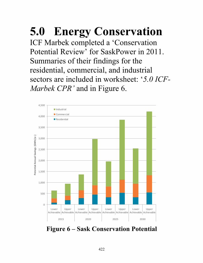
422

5.0 Energy Conservation

ICF Marbek completed a ‘Conservation Potential Review’ for SaskPower in 2011. Summaries of their findings for the residential, commercial, and industrial sectors are included in worksheet: ‘5.0 ICF-Marbek CPR’ and in Figure 6.

Figure 6 – Sask Conservation Potential

SaskPower CPR 2010 Summary Report

ICF Marbek 11

Exhibit 4 Upper and Lower Achievable Electric Energy Savings by Sector

0

500

1,000

1,500

2,000

2,500

3,000

3,500

4,000

4,500

Lower Achievable

Upper Achievable

Lower Achievable

Upper Achievable

Lower Achievable

Upper Achievable

Lower Achievable

Upper Achievable

2015 2020 2025 2030

Pote

ntia

l Ann

ual S

avin

gs (

GW

h/yr

.)

Industrial

Commercial

Residential

423

To understand the costs of undertaking energy conservation in Saskatchewan I looked to the Ontario Conservation Potential Review (CPR) also written by ICF-Marbek. The Ontario documents provide cost information including the expected program costs that would be spent to achieve certain levels of energy conservation. I used the Ontario cost data and scaled it to match the Saskatchewan conservation potential. I then estimated a linear relationship between electricity savings and program costs. Figures 7-9 summarize the relationships.

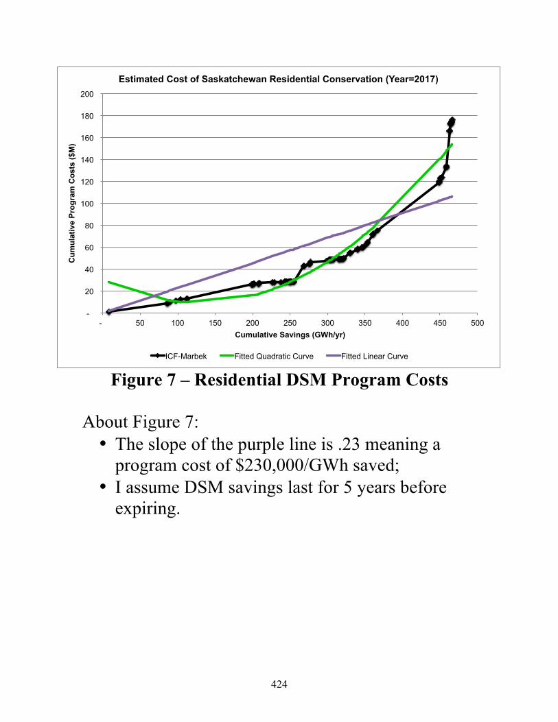
424

Figure 7 – Residential DSM Program Costs

About Figure 7: • The slope of the purple line is .23 meaning a

program cost of $230,000/GWh saved; • I assume DSM savings last for 5 years before

expiring.

-

20

40

60

80

100

120

140

160

180

200

- 50 100 150 200 250 300 350 400 450 500

Cum

ulat

ive

Pro

gram

Cos

ts ($

M)

Cumulative Savings (GWh/yr)

Estimated Cost of Saskatchewan Residential Conservation (Year=2017)

ICF-Marbek Fitted Quadratic Curve Fitted Linear Curve

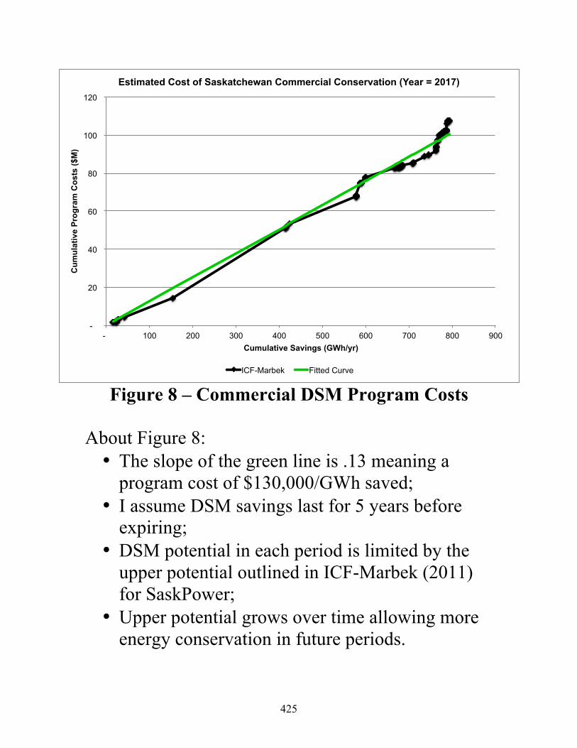
425

Figure 8 – Commercial DSM Program Costs

About Figure 8: • The slope of the green line is .13 meaning a

program cost of $130,000/GWh saved; • I assume DSM savings last for 5 years before

expiring; • DSM potential in each period is limited by the

upper potential outlined in ICF-Marbek (2011) for SaskPower;

• Upper potential grows over time allowing more energy conservation in future periods.

-

20

40

60

80

100

120

- 100 200 300 400 500 600 700 800 900

Cum

ulat

ive

Pro

gram

Cos

ts ($

M)

Cumulative Savings (GWh/yr)

Estimated Cost of Saskatchewan Commercial Conservation (Year = 2017)

ICF-Marbek Fitted Curve

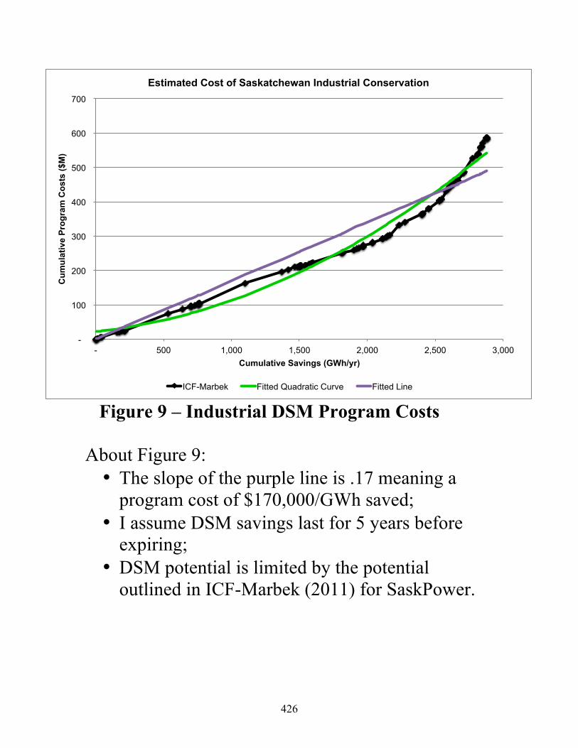
426

Figure 9 – Industrial DSM Program Costs

About Figure 9: • The slope of the purple line is .17 meaning a

program cost of $170,000/GWh saved; • I assume DSM savings last for 5 years before

expiring; • DSM potential is limited by the potential

outlined in ICF-Marbek (2011) for SaskPower.

-

100

200

300

400

500

600

700

- 500 1,000 1,500 2,000 2,500 3,000

Cum

ulat

ive

Pro

gram

Cos

ts ($

M)

Cumulative Savings (GWh/yr)

Estimated Cost of Saskatchewan Industrial Conservation

ICF-Marbek Fitted Quadratic Curve Fitted Line

427

In the ICF-Marbek reports, program costs per Gigawatt-hour saved begin to increase with higher energy conservation achievement. This reflects the need to pay more for incentives to encourage conserving actions. To keep the model linear I used the upper technical potential numbers as hard constraints on the potential DSM in each investment period and kept the program costs constant over time. Please consider the following questions: Q6. Is it valid to draw upon Ontario’s program costs when analyzing Saskatchewan’s conservation costs?

428

Q7. Is it valid to use constant program costs up to a hard limit in each period? Q8. Are the program costs ($/GWh saved) accurate? Note that they do not change over time. This assumes that ‘low-hanging fruit’ appears as quickly as we can ‘pick it’.

429

Peak Demand Savings Energy saved (measured in Gigawatt-hours) is converted into peak demand savings using different formulas for residential, commercial, and industrial savings. Conversion factors are highlighted in yellow in the worksheet: ‘5.0 ICF-Marbek CPR’. The conversion factors were selected to calibrate to the ICF-Marbek relationship between GWh saved and peak demand shaved. I assume that industrial peak demand reduction is half that of the ICF-Marbek report. Q9. Is this a valid method of estimating peak demand reduction?

430

References for Appendix 9C

EIA (2015) Assumptions to the Annual Energy Outlook 2014 – Electricity Market Module.

EIA (2014b) Assumptions to the Annual Energy Outlook 2014 – Appendix: Tables for 2040 (Table A5). Retrieved from: http://www.eia.gov/forecasts/aeo/pdf/appendix_tbls.pdf, Last accessed October 1, 2014.

ICF-Marbek (2011) SaskPower Conservation Potential Review Summary Report. Regina, SK: SaskPower.

ICF-Marbek (2010a) Achievable Potential - Residential Sector Final Report - Estimated Range of Electricity Savings Through Future OntarioConservation Programs. Ontario Power Authority (OPA).

ICF-Marbek (2010b) Achievable Potential - Commercial Sector Final Report - Estimated Range of Electricity Savings Through Future Ontario Conservation Programs. Ontario Power Authority (OPA).

ICF-Marbek (2010b) Achievable Potential - Industrial Sector Final Report - Estimated Range of Electricity Savings Through Future Ontario Conservation Programs. Ontario Power Authority (OPA).

NEB (National Energy Board) (2013) Canada’s Energy Future 2013: Energy Supply and Demand Projections to 2035. Ottawa, ON: National Energy Board.

SaskPower (2014b) 2014 Load Forecast. SaskPower Load & Revenue Forecasting. Regina SK.

Thank-you for agreeing to participate in an energy-modelling workshop focused on ‘Opportunitiesand Barriers for Renewable Energy and Energy Conservation in Saskatchewan.’ This survey isbeing used to get a sense of the range of perspectives that will be present at the workshop.

Please answer the 8 questions below. This survey should take 10-12 minutes to complete.

Note that your responses will not be attributed to you personally and your identity will be kept inconfidence. Your responses will be made anonymous and presented at the workshop along withthe responses provided by the other participants.

Thank-you for your time,Brett DolterPhD researcherYork Universitybrett.dolter@gmail.com

Pre-Workshop Survey

Renewable Electricity in Saskatchewan

1

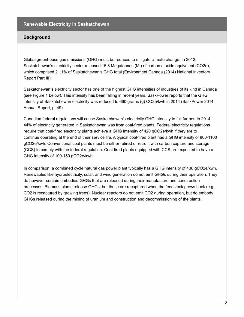
Background

Renewable Electricity in Saskatchewan

Global greenhouse gas emissions (GHG) must be reduced to mitigate climate change. In 2012,Saskatchewan's electricity sector released 15.8 Megatonnes (Mt) of carbon dioxide equivalent (CO2e),which comprised 21.1% of Saskatchewan’s GHG total (Environment Canada (2014) National InventoryReport Part III).

Saskatchewan’s electricity sector has one of the highest GHG intensities of industries of its kind in Canada(see Figure 1 below). This intensity has been falling in recent years. SaskPower reports that the GHGintensity of Saskatchewan electricity was reduced to 660 grams (g) CO2e/kwh in 2014 (SaskPower 2014Annual Report, p. 49).

Canadian federal regulations will cause Saskatchewan's electricity GHG intensity to fall further. In 2014,44% of electricity generated in Saskatchewan was from coal-fired plants. Federal electricity regulationsrequire that coal-fired electricity plants achieve a GHG intensity of 420 gCO2e/kwh if they are tocontinue operating at the end of their service life. A typical coal-fired plant has a GHG intensity of 800-1100gCO2e/kwh. Conventional coal plants must be either retired or retrofit with carbon capture and storage(CCS) to comply with the federal regulation. Coal-fired plants equipped with CCS are expected to have aGHG intensity of 100-150 gCO2e/kwh.

In comparison, a combined cycle natural gas power plant typically has a GHG intensity of 436 gCO2e/kwh.Renewables like hydroelectricity, solar, and wind generation do not emit GHGs during their operation. Theydo however contain embodied GHGs that are released during their manufacture and constructionprocesses. Biomass plants release GHGs, but these are recaptured when the feedstock grows back (e.g.CO2 is recaptured by growing trees). Nuclear reactors do not emit CO2 during operation, but do embodyGHGs released during the mining of uranium and construction and decommissioning of the plants.

2

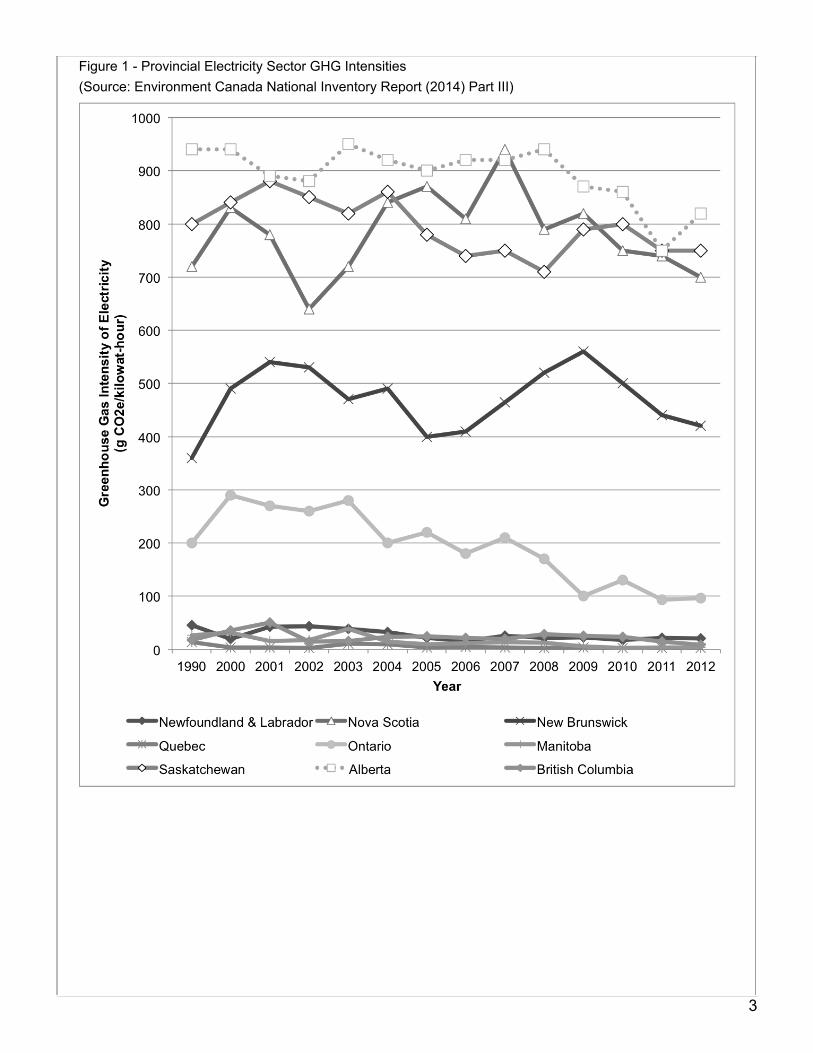
Figure 1 - Provincial Electricity Sector GHG Intensities (Source: Environment Canada National Inventory Report (2014) Part III)

3

Question 1 - Long-Term Target for the GHG Intensity of Saskatchewan Electricity

Renewable Electricity in Saskatchewan

Comment

1. Thinking ahead to the future, what GHG intensity should Saskatchewan strive to achieve in the electricitysector by 2050?

*

900-999 gCO2e/kwh

800-899 gCO2e/kwh

700-799 gCO2e/kwh

600-699 gCO2e/kwh

500-599 gCO2e/kwh

400-499 gCO2e/kwh

300-399 gCO2e/kwh

200-299 gCO2e/kwh

100-199 gCO2e/kwh

0-99 gCO2e/kwh

Uncertain - don't want to hazard a guess

Don't Know

4

Question 2 - Technologies for Reducing Saskatchewan Electricity GHG Intensity

Renewable Electricity in Saskatchewan

5

2. Several technologies might contribute to lowering the GHG intensity of Saskatchewan's electricitysystem. Seventeen of these technologies are listed below in alphabetical order. Please rank thetechnologies in terms of their importance for reducing the GHG intensity of Saskatchewan's electricitysystem, with 1 indicating most important and 17 indicating least important. Note: You can drag and dropeach listed technology to the position you like.

Battery storage (e.g. lithium-ion, hydrogen) N/A

Biomass N/A

Coal with Carbon Capture & Storage (CCS) N/A

Demand Side Management (e.g. peak load shifting, energy conservation, smart grids) N/A

Hydroelectricity (Saskatchewan) N/A

Hydroelectric imports from Manitoba N/A

Natural Gas Cogeneration (partner with industry e.g. potash mining) N/A

Natural Gas Combined Cycle N/A

Natural Gas Simple Cycle N/A

Natural Gas with Carbon Capture and Storage (CCS) N/A

Pumped Hydro Electricity Storage N/A

Small Modular Nuclear Reactors (360 MW or smaller) N/A

Solar Photovoltaics (small-scale distributed generation <10 MW) N/A

Solar Photovoltaics (utility-scale 10 MW or greater) N/A

Solar Thermal (utility-scale 10 MW or greater) N/A

Wind (small-scale distributed generation, turbines <1 MW) N/A

Wind (utility-scale, turbines 1 MW or larger) N/A

6

Question 3 - Preferred Electricity Generation Scenario

Renewable Electricity in Saskatchewan

7

Biomass

Coal-fired Generation with CarbonCapture and Storage (CCS)

Conventional Coal-fired Generation

Demand Side Management (e.g. peakload shifting, energy conservation,smart grid)

Hydroelectricity (Saskatchewan)

Hydroelectric Imports from Manitoba

Natural Gas Cogeneration (partner withindustry e.g. potash mining company)

Natural Gas Combined Cycle

Natural Gas Simple Cycle

Natural Gas with Carbon Capture andStorage (CCS)

Small Modular Nuclear Reactors (360MW or smaller)

Solar Photovoltaics (small-scaledistributed generation <10 MW)

Solar Photovoltaics (utility-scale 10 MWor larger)

Solar Thermal (utility-scale 10 MW orlarger)

Wind (small-scale distributedgeneration, turbines <1 MW)

Wind (utility-scale, turbines 1 MW orlarger)

3. Imagine a preferred electricity generation mix in the year 2050 that achieves the electricity GHG intensityyou listed in Question 1. What proportion of total electricity generation is provided by each of the followingtechnologies in your preferred scenario?

Please respond by typing the desired proportions in the appropriate boxes.

Please respond in terms of proportion of electricity generated (% Gigawatt-hours) rather than proportion ofcapacity installed (% Megawatts).

The choices need to add up to 100.

*

8

Question 4 - Medium-Term Renewable Energy Potential in Saskatchewan

Renewable Electricity in Saskatchewan

Other (please specify)

4. Renewable electricity generation technologies include: biomass, hydroelectric, solar photovoltaic, solarthermal, and wind generation. In 2014, renewables supplied 23% of Saskatchewan's electricity demandwith hydroelectricity providing 20%, wind providing 3%, and small contributions from solar photovoltaicsand biomass.

What is the maximum proportion of Saskatchewan electricity that renewables can supply in the medium-term (i.e. by 2030-2035)?

*

100%

90-99%

80-89%

70-79%

60-69%

50-59%

40-49%

30-39%

20-29%

10-19%

0-9%

9

Question 5 - Long-Term Renewable Electricity Potential in Saskatchewan

Renewable Electricity in Saskatchewan

Other (please specify)

5. What is the maximum proportion of Saskatchewan electricity that renewables can supply in thelong-term (i.e. by 2045-2050)?

*

100%

90-99%

80-89%

70-79%

60-69%

50-59%

40-49%

30-39%

20-29%

10-19%

0-9%

10

Question 6 - Desirable Renewable Electricity Generation Mix

Renewable Electricity in Saskatchewan

11

Biomass

Coal-fired Generation with CarbonCapture and Storage (CCS)

Conventional Coal-fired Generation

Demand Side Management (e.g. peakload shifting, energy conservation,smart grids)

Hydroelectricity (Saskatchewan)

Hydroelectric Imports from Manitoba

Natural Gas Cogeneration (partner withindustry e.g. potash mining company)

Natural Gas Combined Cycle

Natural Gas Simple Cycle

Natural Gas with Carbon Capture andStorage (CCS)

Small Modular Nuclear Reactors (360MW of smaller)

Solar Photovoltaics (small-scaledistributed generation < 10 MW)

Solar Photovoltaics (utility-scale 10 MWor larger)

Solar Thermal (utility-scale 10 MW orlarger)

Wind (small-scale distributedgeneration, turbines <1 MW)

Wind Power (utility-scale, turbineslarger than 1 MW)

6. What electricity generation mix would achieve the maximum renewable potential you identified inQuestion 5?

Please indicate the proportion of electricity generated by each of the following technologies in the long-runmaximum renewable potential scenario.

Please respond in terms of proportion of electricity generated (% Gigawatt-hours) rather than proportionof capacity installed (% Megawatts).

The choices need to add up to 100. If necessary, please include non-renewable elements that would becomplementary to the renewable contributions to take the total to 100.

*

12

Question 7 - Barriers to Renewable Electricity

Renewable Electricity in Saskatchewan

Not importantSomewhatimportant Very important

Cost: The price of renewable electricity is too high.

Feed-in-Tariff: Saskatchewan does not pay preferred rates for renewablepower.

Grid design: The Saskatchewan grid is built for centralized, not distributed,generation.

Job loss: A focus on renewables will lead to lost jobs in the coal-powerindustry.

Intermittency: Renewables cannot provide reliable electricity.

Physical limits: Saskatchewan lacks adequate hydro, solar, wind resources.

Political will: Political leaders in Saskatchewan have not prioritizedrenewables.

Preference for coal: SaskPower has a preference for coal-fired generation.

Public ownership: A private market would increase renewables more quickly.

Social acceptance: People do not want to live near renewable energygeneration.

Other (please specify)

7. In speaking to diverse stakeholders about the future of electricity in Saskatchewan I heard about barriersto increasing renewable electricity in Saskatchewan. Participants in the interviews listed the followingbarriers. How important is each barrier?

13

Respondent Information

Renewable Electricity in Saskatchewan

Name

Company/Affiliation

Email Address

Phone Number

8. Please provide your name, affiliation, and a means of contacting you. *

14

Thank-you!

Renewable Electricity in Saskatchewan

15