graviton-induced bremsstrahlung at e + e - colliders
TRANSCRIPT
arX
iv:h
ep-p
h/04
0326
7v1
25
Mar
200
4
March 2004
Graviton-induced Bremsstrahlung at e+e− colliders
Trygve Buanes∗, Erik W. Dvergsnes†, Per Osland‡
Department of Physics and Technology, University of Bergen,
Allegaten 55, N-5007 Bergen, Norway
Abstract
We consider graviton-induced Bremsstrahlung at future e+e− colliders in both the ADDand RS models, with emphasis on the photon perpendicular momentum and angular dis-tribution. The photon spectrum is shown to be harder than in the Standard Model, andthere is an enhancement for photons making large angles with respect to the beam. In theADD scenario, the excess at large photon perpendicular momenta should be measurable forvalues of the cut-off up to about twice times the c.m. energy. In the RS scenario, radiativereturn to graviton resonances below the c.m. energy can lead to large enhancements of thecross section.

1 Introduction
Early ideas on brane world scenarios date back to more than 15 years ago [1, 2]. In recentyears, more predictive and explicit scenarios involving extra dimensions have been proposed[3–7]. As opposed to string theory with tiny compactification scales of O(10−35 m), thereis now a large number of theories which actually will be tested in the current and nextgeneration of experiments.
Here we shall consider two of these scenarios, namely the Arkani-Hamed–Dimopoulos–Dvali (ADD) [3] and the Randall–Sundrum (RS) scenario [6], and investigate some sig-nals characteristic of such models at possible future electron–positron linear colliders likeTESLA [8] and CLIC [9].
The most characteristic feature of these models is that they predict the existence ofmassive gravitons, which may either be emitted into the final state (leading to events withmissing energy and momentum), or exchanged as virtual, intermediate states. We shallhere focus on the effects of such massive graviton exchange on the Bremsstrahlung process:
e+e− → µ+µ−γ, (1.1)
for which the basic electroweak contributions are well known [10].Due to an extra photon in the final state, this process has a reduced cross section as
compared to two-body final states like µ+µ− and γγ, and is unlikely to be the discoverychannel, but it may provide additional confirmation if a signal should be observed in thetwo-body final states. In particular, the presence of additional Feynman diagrams, withoutthe infrared and collinear singularities of the Standard Model (SM) leads one to expect aharder photon spectrum.
We shall first, in Sect. 2, present the differential cross section for the process (1.1). Inte-grated cross sections as well as photon perpendicular momentum and angular distributionswill be discussed. Then, in Sects. 3 and 4, we specialize to the ADD and RS scenarios, byperforming sums over the respective KK towers. In Sect. 5 we summarize our conclusions.
2 Graviton induced Bremsstrahlung
In this section we present the cross section for the process (1.1), taking into account thes-channel exchange of the photon, the Z and a single graviton of mass m~n and width Γ~n.These results are for the differential cross section very similar to those obtained for gravitonexchange in the analogous process qq → e+e−γ [11], and will in Sects. 3 and 4 be adaptedto the ADD and RS scenarios.
2.1 Differential cross sections
The cross section for the process in Eq. (1.1) is determined by the Feynman diagrams ofFig. 1 (“set A”, initial state radiation, ISR) and Fig. 2 (“set B”, final state radiation,FSR), in addition to the well known SM diagrams which are obtained by substituting the
2
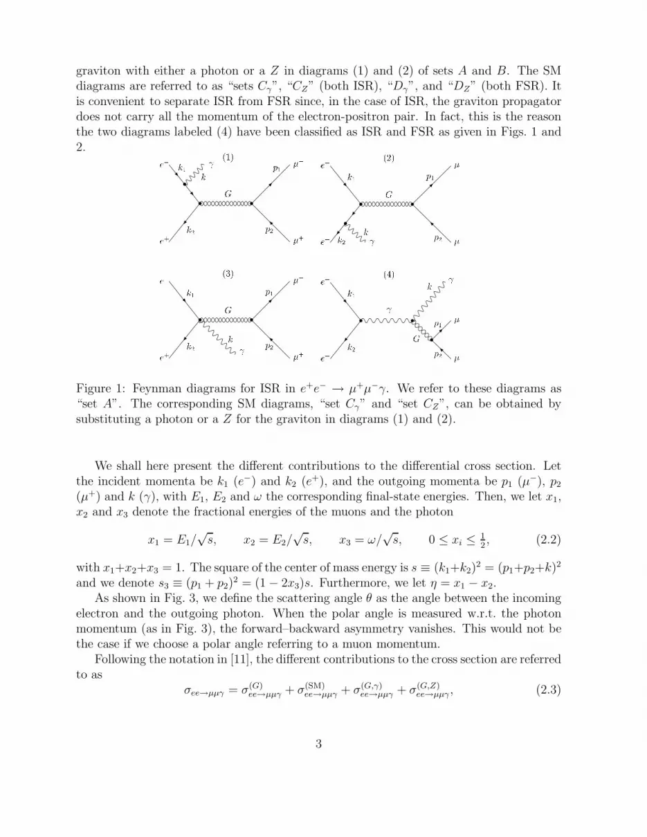
graviton with either a photon or a Z in diagrams (1) and (2) of sets A and B. The SMdiagrams are referred to as “sets Cγ”, “CZ” (both ISR), “Dγ”, and “DZ” (both FSR). Itis convenient to separate ISR from FSR since, in the case of ISR, the graviton propagatordoes not carry all the momentum of the electron-positron pair. In fact, this is the reasonthe two diagrams labeled (4) have been classified as ISR and FSR as given in Figs. 1 and2. e�
e+k1k2
(1)G ���+
k p1p2
e�e+
k1k2
(2)G
��k �+
p1p2e�
e+k1k2
(3)G ���+k
p1p2
e�e+
k1k2
(4) G k ���+p1p2
Figure 1: Feynman diagrams for ISR in e+e− → µ+µ−γ. We refer to these diagrams as“set A”. The corresponding SM diagrams, “set Cγ” and “set CZ”, can be obtained bysubstituting a photon or a Z for the graviton in diagrams (1) and (2).
We shall here present the different contributions to the differential cross section. Letthe incident momenta be k1 (e−) and k2 (e+), and the outgoing momenta be p1 (µ−), p2
(µ+) and k (γ), with E1, E2 and ω the corresponding final-state energies. Then, we let x1,x2 and x3 denote the fractional energies of the muons and the photon
x1 = E1/√
s, x2 = E2/√
s, x3 = ω/√
s, 0 ≤ xi ≤ 12, (2.2)
with x1+x2+x3 = 1. The square of the center of mass energy is s ≡ (k1+k2)2 = (p1+p2+k)2
and we denote s3 ≡ (p1 + p2)2 = (1 − 2x3)s. Furthermore, we let η = x1 − x2.
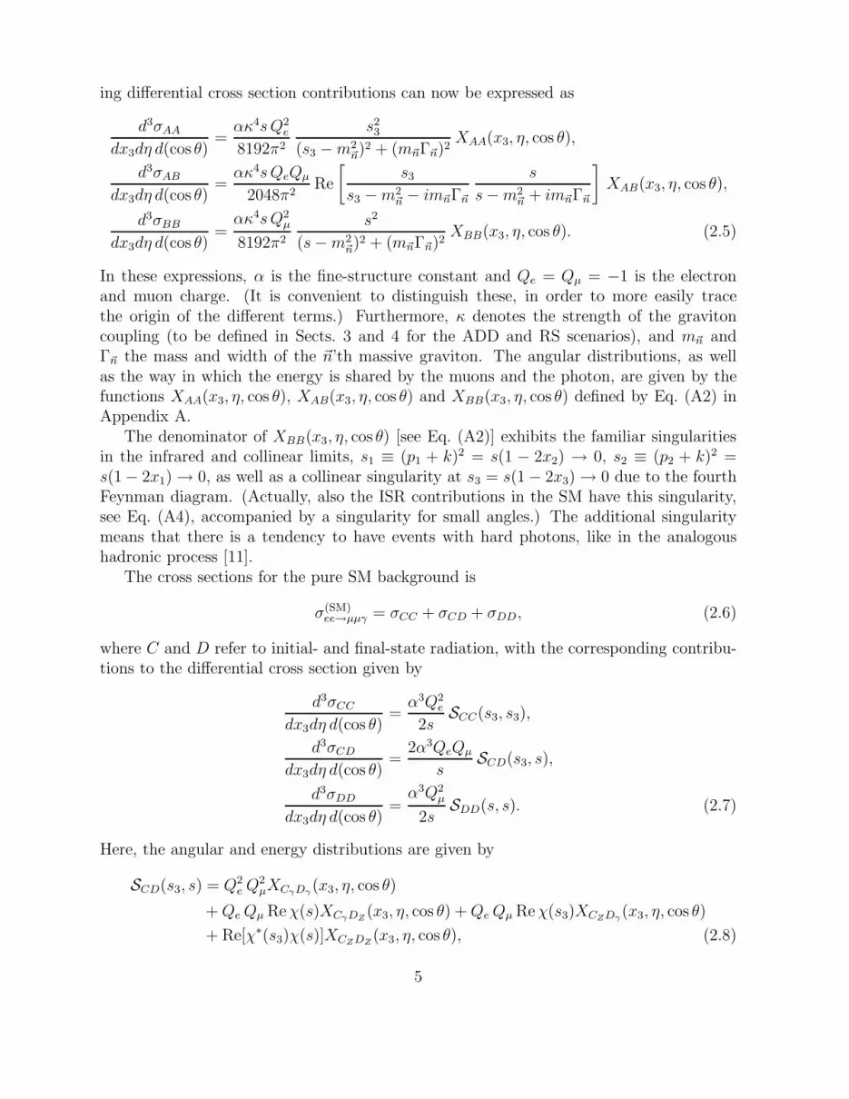
As shown in Fig. 3, we define the scattering angle θ as the angle between the incomingelectron and the outgoing photon. When the polar angle is measured w.r.t. the photonmomentum (as in Fig. 3), the forward–backward asymmetry vanishes. This would not bethe case if we choose a polar angle referring to a muon momentum.
Following the notation in [11], the different contributions to the cross section are referredto as
σee→µµγ = σ(G)ee→µµγ + σ(SM)
ee→µµγ + σ(G,γ)ee→µµγ + σ(G,Z)
ee→µµγ , (2.3)
3
e�e+
k1k2
(1)G ���+kp1p2e�e+
k1k2
(2)G ���+kp1p2e�
e+k1k2
(3)G ���+kp1p2
e�e+
k1k2
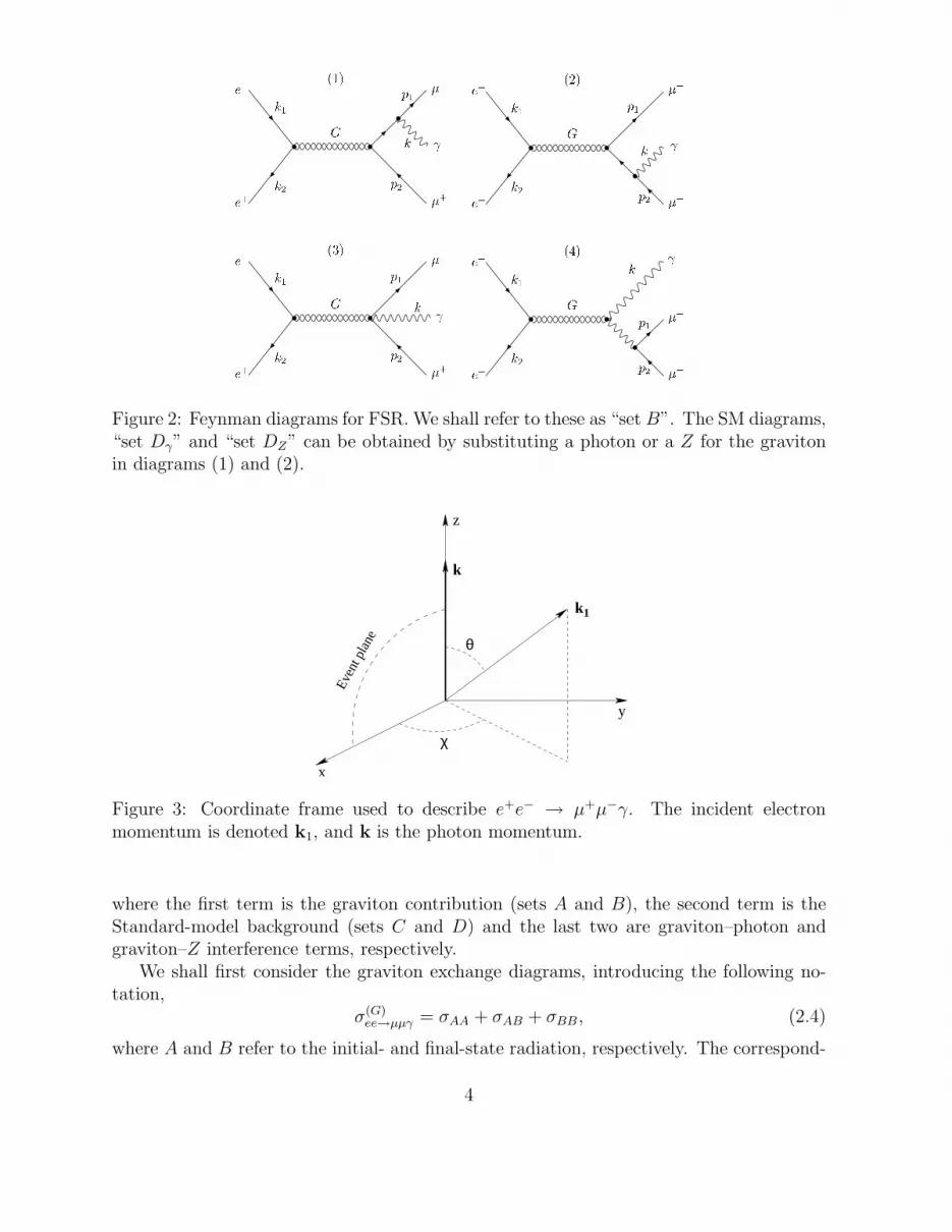
(4)G k ���+p1p2Figure 2: Feynman diagrams for FSR. We shall refer to these as “set B”. The SM diagrams,“set Dγ” and “set DZ” can be obtained by substituting a photon or a Z for the gravitonin diagrams (1) and (2).
Even
t pla
ne
x
y
z
θ
k
k1
χ
Figure 3: Coordinate frame used to describe e+e− → µ+µ−γ. The incident electronmomentum is denoted k1, and k is the photon momentum.
where the first term is the graviton contribution (sets A and B), the second term is theStandard-model background (sets C and D) and the last two are graviton–photon andgraviton–Z interference terms, respectively.
We shall first consider the graviton exchange diagrams, introducing the following no-tation,
σ(G)ee→µµγ = σAA + σAB + σBB , (2.4)
where A and B refer to the initial- and final-state radiation, respectively. The correspond-
4
ing differential cross section contributions can now be expressed as
d3σAA
dx3dη d(cos θ)=
ακ4s Q2e
8192π2
s23
(s3 − m2~n)2 + (m~nΓ~n)2
XAA(x3, η, cos θ),
d3σAB
dx3dη d(cos θ)=
ακ4s QeQµ
2048π2Re
[
s3
s3 − m2~n − im~nΓ~n
s
s − m2~n + im~nΓ~n
]
XAB(x3, η, cos θ),
d3σBB
dx3dη d(cos θ)=
ακ4s Q2µ
8192π2
s2
(s − m2~n)2 + (m~nΓ~n)2
XBB(x3, η, cos θ). (2.5)
In these expressions, α is the fine-structure constant and Qe = Qµ = −1 is the electronand muon charge. (It is convenient to distinguish these, in order to more easily tracethe origin of the different terms.) Furthermore, κ denotes the strength of the gravitoncoupling (to be defined in Sects. 3 and 4 for the ADD and RS scenarios), and m~n andΓ~n the mass and width of the ~n’th massive graviton. The angular distributions, as wellas the way in which the energy is shared by the muons and the photon, are given by thefunctions XAA(x3, η, cos θ), XAB(x3, η, cos θ) and XBB(x3, η, cos θ) defined by Eq. (A2) inAppendix A.
The denominator of XBB(x3, η, cos θ) [see Eq. (A2)] exhibits the familiar singularitiesin the infrared and collinear limits, s1 ≡ (p1 + k)2 = s(1 − 2x2) → 0, s2 ≡ (p2 + k)2 =s(1 − 2x1) → 0, as well as a collinear singularity at s3 = s(1 − 2x3) → 0 due to the fourthFeynman diagram. (Actually, also the ISR contributions in the SM have this singularity,see Eq. (A4), accompanied by a singularity for small angles.) The additional singularitymeans that there is a tendency to have events with hard photons, like in the analogoushadronic process [11].
The cross sections for the pure SM background is
σ(SM)ee→µµγ = σCC + σCD + σDD, (2.6)
where C and D refer to initial- and final-state radiation, with the corresponding contribu-tions to the differential cross section given by
d3σCC
dx3dη d(cos θ)=
α3Q2e
2sSCC(s3, s3),
d3σCD
dx3dη d(cos θ)=
2α3QeQµ
sSCD(s3, s),
d3σDD
dx3dη d(cos θ)=
α3Q2µ
2sSDD(s, s). (2.7)
Here, the angular and energy distributions are given by
SCD(s3, s) = Q2e Q2
µXCγDγ (x3, η, cos θ)
+ Qe Qµ Re χ(s)XCγDZ(x3, η, cos θ) + Qe Qµ Re χ(s3)XCZDγ (x3, η, cos θ)
+ Re[χ∗(s3)χ(s)]XCZDZ(x3, η, cos θ), (2.8)
5
with SCC(s3, s3) and SDD(s, s) similarly obtained from Eq. (2.8) by substituting (D, s) ↔(C, s3). Furthermore, the XCγDγ etc. are given by Eq. (A4) and the Z propagator isrepresented by
χ(s) =1
sin2(2θW )
s
(s − m2Z) + imZΓZ
, (2.9)
with mZ and ΓZ the mass and width of the Z boson, and θW the weak mixing angle. Notethat σCγCZ
= σCZCγ and σDγDZ= σDZDγ .
For the interference terms between graviton exchange and the SM diagrams, we intro-duce the following notation:
σ(G,γ)ee→µµγ = σACγ + σBDγ + σADγ + σBCγ ,
σ(G,Z)ee→µµγ = σACZ
+ σBDZ+ σADZ
+ σBCZ. (2.10)
Like above, the subscripts indicate the diagram sets involved. The corresponding differen-tial cross section contributions are given by
d3σACγ
dx3dη d(cos θ)=
α2κ2 Q3eQµ
32πRe
[
s3
s3 − m2~n + im~nΓ~n
]
XACγ (x3, η, cos θ),
d3σACZ
dx3dη d(cos θ)=
α2κ2 Q2e
64πRe
[
χ∗(s3)s3
s3 − m2~n + im~nΓ~n
]
XACZ(x3, η, cos θ),
d3σBDγ
dx3dη d(cos θ)=
α2κ2 QeQ3µ
32πRe
[
s
s − m2~n + im~nΓ~n
]
XBDγ (x3, η, cos θ),
d3σBDZ
dx3dη d(cos θ)=
α2κ2 Q2µ
64πRe
[
χ∗(s)s
s − m2~n + im~nΓ~n
]
XBDZ(x3, η, cos θ),
d3σADγ
dx3dη d(cos θ)=
α2κ2 Q2eQ
2µ
128πRe
[
s3
s3 − m2~n + im~nΓ~n
]
XADγ (x3, η, cos θ),
d3σADZ
dx3dη d(cos θ)=
α2κ2 QeQµ
128πRe
[
χ∗(s)s3
s3 − m2~n + im~nΓ~n
]
XADZ(x3, η, cos θ),
d3σBCγ
dx3dη d(cos θ)=
α2κ2 Q2eQ
2µ
128πRe
[
s
s − m2~n + im~nΓ~n
]
XBCγ (x3, η, cos θ),
d3σBCZ
dx3dη d(cos θ)=
α2κ2 QeQµ
128πRe
[
χ∗(s3)s
s − m2~n + im~nΓ~n
]
XBCZ(x3, η, cos θ). (2.11)
The XACγ etc. are given in Appendix A.An overview of the notations used for the different contributions to the cross section is
given in Table 1.
6

ISR FSRG Z G ZISRFSR
G ZG Z
AA AC ACZ AB AD ADZC C C CZ BC C D C DZCZCZ BCZ CZD CZDZBB BD BDZD D D DZDZDZTable 1: Notation used for different combinations of amplitudes. Compare the labeling ofdiagrams in Figs. 1 and 2.
2.2 Total cross section
To obtain the total cross section, we integrate the differential cross section presented inSec. 2.1 within the following limits:
σee→µµγ =
∫ 1−ccut
−1+ccut
d(cos θ)
∫ xmax
3
xmin
3
dx3
∫ x3−ycut
−x3+ycut
dηd3σee→µµγ
dx3dη d(cos θ). (2.12)
Since the detector has a ‘blind’ region very close to the beam pipe, we impose a cut,| cos θ| < 1 − ccut, with ccut = 0.005, which translates into a lower bound on sin θmin ≃ 0.1or an angular cut of θmin ≃ 100 mrad. This cut removes the singularity due to initial-stateradiation (recall that θ is the angle between the photon and the incident beam).
The resolution cut, ycut = 0.005, is imposed to exclude collinear events, i.e., by requiringsi = (1 − 2xi)s > ycut s. For fixed x3, this leads to |η| < x3 − ycut, where η = x1 − x2. Thevariable x3 is bounded by the allowed values of si, giving ycut < x3 < 1
2(1 − ycut) ≡ xmax
3 .As a result of the cut on si, the minimal photon momentum is kmin = ycut
√s. For√
s = 500 GeV and the chosen value for ycut, this becomes 2.5 GeV. In addition to this cutwe shall also require that the photon perpendicular momentum is subject to an absolute cut,k⊥ = k sin θ > kmin
⊥ . Here we choose kmin⊥ = ξcut
√s, with ξcut = 0.005. For
√s = 500 GeV,
kmin⊥ = 2.5 GeV, which means that photons with momentum kmin only survive this cut
when sin θ = 1. If sin θ = sin θmin, only photons of k > 25 GeV survive the cuts.When expressed in terms of the variables x3 and cos θ, the k⊥ constraint becomes
7
x3
√1 − cos2 θ > ξcut. Thus, for a given cos θ in the allowed range, we find
x3 > xmin3 = max
(
ξcut√1 − cos2 θ
, ycut
)
(2.13)
In order to exclude radiative return to the Z, we will also consider the cut
s3 > (mZ + 3ΓZ)2 ≡ yrrcuts. (2.14)
This implies
yrrcut =
m2Z
s
(
1 +3ΓZ
mZ
)2
≃ 1.17 × m2Z
s, (2.15)
which for√
s = 500 GeV gives yrrcut ≃ 0.039. This value will modify the upper bound xmax
3 ,which will become 1
2(1 − yrr
cut), but not affect the lower bound, xmin3 , nor the limits on η.
2.3 Photon perpendicular momentum distribution
It is instructive to consider the spectrum of the photon perpendicular momentum, k⊥, sincethis has no analogue in the two-body final state process. As anticipated above, we expect itto be harder than in the QED case. The relevant differential cross sections can be obtainedfrom the expressions in Sec. 2.1 upon a change of variables from (x3, cos θ) → (k⊥, k‖). Fromthe definitions, k⊥ =
√sx3 sin θ and k‖ =
√sx3 cos θ, we get dx3d(cos θ) → |J |dk‖dk⊥ with
the Jacobian
|J | =k⊥√sk2
=k⊥√
s(k2⊥ + k2
‖). (2.16)
The photon perpendicular momentum spectrum is now obtained from
dσee→µµγ
dk⊥=
∫ kmax
‖
−kmax
‖
dk‖
∫ x3−ycut
−x3+ycut
dηdσ3
ee→µµγ
dk⊥dk‖dη. (2.17)
Given some k⊥ within the allowed region ξcut
√s < k⊥ <
√s
2(1 − ycut), we find
|k‖| < kmax‖ = min
(√
s
4(1 − ycut)2 − k2
⊥,
√s
2(1 − ycut)(1 − ccut)
)
. (2.18)
The resolution cut, ycut, and also the radiative-return cut, yrrcut, will be the same as for the
total cross section, and the radiative-return cut will affect both kmax⊥ and kmax
‖ .
2.4 Photon angular distribution
For the two-body final states e+e− → µ+µ− and e+e− → γγ, the QED angular distributionsare given by the familiar 1 + cos2 θ and (1 + cos2 θ)/(1 − cos2 θ). For graviton exchange,the corresponding distributions become 1− 3 cos2 θ + 4 cos4 θ and 1− cos4 θ (see e.g. [12]).In both these cases, the higher powers are due to the spin-2 coupling. For the three-body
8
case, we get similar expressions (see the Appendix). Note that the ISR contribution hasa structure similar to that of the diphoton channel, with a 1 − cos2 θ singularity in thedenominator, whereas graviton exchange gives quartic terms in cos θ.
In order to emphasize the photons originating from graviton exchange over those fromthe collinear singularities (dominated by the SM contributions), we will here consider theangular distribution of the photon with respect to the incident beam:
dσee→µµγ
d(cos θ)=
∫ xmax
3
xmin
3
dx3
∫ x3−ycut
−x3+ycut
dηd3σee→µµγ
dx3dη d(cos θ), (2.19)
with the cuts as given above.
3 The ADD scenario
We first turn our attention to the ADD scenario [3], where there is essentially a continuumof massive graviton states up to some cut-off MS, where a more fundamental theory,presumably low-scale string physics, takes over. Following the convention of [13], thecoherent sum over all KK modes in a tower is performed by substituting for the sum overgraviton propagators the following expression:
κ2
s − m2~n + im~nΓ~n
≡ −iκ2D(s) −→∑
~n
8πsn/2−1
Mn+2S
[2I(MS/√
s) − iπ], (3.20)
with
I(MS/√
s) =
−n/2−1∑
k=1
1
2k
(
MS√s
)2k
− 1
2log
(
M2S
s− 1
)
, n = even,
−(n−1)/2∑
k=1
1
2k − 1
(
MS√s
)2k−1
+1
2log
(
MS +√
s
MS −√s
)
, n = odd.
(3.21)
for n extra dimensions.Since the role of higher-order loop effects is rather unknown [14], these expressions
should not be taken too literally. However, in order to preserve the qualitative differencebetween the two propagators D(s) and D(s3) (see Eq. (3.20)), and thus more easily keeptrack of the contributions of different Feynman diagrams, we shall use the expressions ofEq. (3.21). In the approach of [15] and [16] the n-dependence is absorbed in the cut-off sothat D(s) and D(s3) are indistinguishable. For n = 4 and MS ≫ √
s, the cut-off MS iscomparable to ΛT of ref. [15] and MH of [16].
3.1 Total cross sections
In Figs. 4 and 5, we present the total cross section [see Eq. (2.12)] vs. the UV cut-off MS,for n = 2, 4 and 6. (For n = 2, this range of MS is actually in conflict with astrophysical
9

5060708090
100
200
300
400
500
n=2
46
n=2
46
Radiative return excluded
MS [TeV]
σ [f
b]
ADD+SM
SM
1 1.5 2 2.5 3
ADDs=0.5 TeV√
10
10 2
10 3
Radiative return to Z excluded
MS [TeV]
σ [f
b]
ADD+SM
SM
1.5 2 2.5 3 3.5 4
ADDs=1 TeV√
Figure 4: Total cross sections for e+e− → µ+µ−γ vs. MS, for√
s = 0.5 and 1 TeV, andn = 2, 4 and 6, with (solid) and without (dashed) radiative return to the Z pole. The SMvalue is represented by a band corresponding to Lint = 300 fb−1.
1
10
10 2
n=2
n=6
MS [TeV]
σ [f
b]
ADD+SM
SM
4 5 6 7 8
ADDs=3 TeV√
102
10
1
10-1
n=2
n=6
MS [TeV]
σ [f
b]ADD+SM
SM
6 8 10 12
ADDs=5 TeV√
Figure 5: Total cross sections for e+e− → µ+µ−γ vs. MS , for√
s = 3 and 5 TeV, andn = 2, 4, and 6. The SM value is represented by a band corresponding to Lint = 1000 fb−1.
data [17].) Different collider energies are considered,√
s = 0.5 and 1.0 TeV in Fig. 4, and3.0 and 5.0 TeV in Fig. 5. For
√s = 3 and 5 TeV, radiative return to Z is already excluded
by the y cut, and therefore only one set of curves is shown.It is seen that the integrated cross sections can have a significant enhancement over the
SM result provided MS is not too much above the actual c.m. energy. Also, we note thatremoving the radiative return to the Z according to the criterion (2.14), the cross section isreduced significantly. Since this mostly affects the SM background, the relative magnitudeof the “signal” increases.
As a rough indication of the precision to be expected, we display the 1σ statistical error
10
band around the SM values, corresponding to an integrated luminosity of 300 fb−1 for thecases of
√s = 0.5 and 1 TeV, and 1000 fb−1 for
√s = 3 and 5 TeV (we take the efficiency
to be 1 throughout the paper). We note that the sensitivity of the integrated cross sectionextends out to values of
√s that are a few times the available c.m. energy. However, since
it is a higher-order process, suppressed by a factor of the order α/π, the sensitivity doesnot compete with that of the two-body final states [16, 18, 19].
3.2 Photon perpendicular momentum distributions
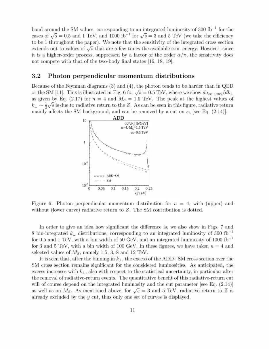
Because of the Feynman diagrams (3) and (4), the photon tends to be harder than in QEDor the SM [11]. This is illustrated in Fig. 6 for
√s = 0.5 TeV, where we show dσee→µµγ/dk⊥
as given by Eq. (2.17) for n = 4 and MS = 1.5 TeV. The peak at the highest values ofk⊥ ∼ 1
2
√s is due to radiative return to the Z. As can be seen in this figure, radiative return
mainly affects the SM background, and can be removed by a cut on s3 [see Eq. (2.14)].
10
1
10-1
10-2
dσ/dk [fb/GeV]⊥
ADD+SM
SM
k [TeV]⊥
0 0.05 0.1 0.15 0.2 0.25
ADD
n=4, MS=1.5 TeVs=0.5 TeV√
Figure 6: Photon perpendicular momentum distribution for n = 4, with (upper) andwithout (lower curve) radiative return to Z. The SM contribution is dotted.
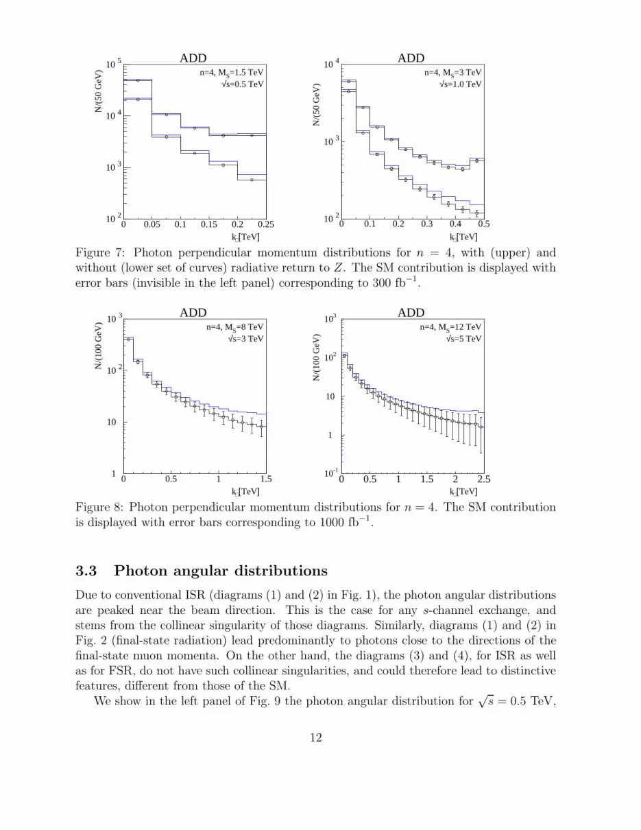
In order to give an idea how significant the difference is, we also show in Figs. 7 and8 bin-integrated k⊥ distributions, corresponding to an integrated luminosity of 300 fb−1
for 0.5 and 1 TeV, with a bin width of 50 GeV, and an integrated luminosity of 1000 fb−1
for 3 and 5 TeV, with a bin width of 100 GeV. In these figures, we have taken n = 4 andselected values of MS, namely 1.5, 3, 8 and 12 TeV.
It is seen that, after the binning in k⊥, the excess of the ADD+SM cross section over theSM cross section remains significant for the considered luminosities. As anticipated, theexcess increases with k⊥, also with respect to the statistical uncertainty, in particular afterthe removal of radiative-return events. The quantitative benefit of this radiative-return cutwill of course depend on the integrated luminosity and the cut parameter [see Eq. (2.14)]as well as on MS. As mentioned above, for
√s = 3 and 5 TeV, radiative return to Z is
already excluded by the y cut, thus only one set of curves is displayed.
11
10 2
10 3
10 4
10 5
0 0.05 0.1 0.15 0.2 0.25
N/(
50 G
eV)
k [TeV]⊥
ADDn=4, MS=1.5 TeV
s=0.5 TeV√
10 2
10 3
10 4
0 0.1 0.2 0.3 0.4 0.5
N/(
50 G
eV)
k [TeV]⊥
ADDn=4, MS=3 TeV
s=1.0 TeV√
Figure 7: Photon perpendicular momentum distributions for n = 4, with (upper) andwithout (lower set of curves) radiative return to Z. The SM contribution is displayed witherror bars (invisible in the left panel) corresponding to 300 fb−1.
1
10
10 2
10 3
0 0.5 1 1.5
N/(
100
GeV
)
k [TeV]⊥
ADDn=4, MS=8 TeV
s=3 TeV√
103
102
10
1
10-1
0 0.5 1 1.5 2 2.5
N/(
100
GeV
)
k [TeV]⊥
ADDn=4, MS=12 TeV
s=5 TeV√
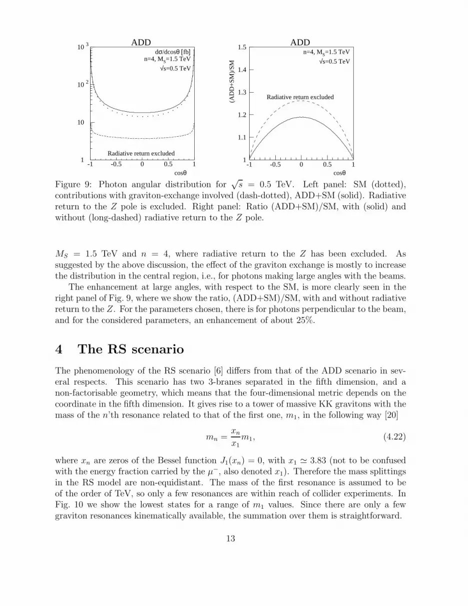
Figure 8: Photon perpendicular momentum distributions for n = 4. The SM contributionis displayed with error bars corresponding to 1000 fb−1.
3.3 Photon angular distributions
Due to conventional ISR (diagrams (1) and (2) in Fig. 1), the photon angular distributionsare peaked near the beam direction. This is the case for any s-channel exchange, andstems from the collinear singularity of those diagrams. Similarly, diagrams (1) and (2) inFig. 2 (final-state radiation) lead predominantly to photons close to the directions of thefinal-state muon momenta. On the other hand, the diagrams (3) and (4), for ISR as wellas for FSR, do not have such collinear singularities, and could therefore lead to distinctivefeatures, different from those of the SM.
We show in the left panel of Fig. 9 the photon angular distribution for√
s = 0.5 TeV,
12
1
10
10 2
10 3
dσ/dcosθ [fb]
Radiative return excluded
cosθ-1 -0.5 0 0.5 1
ADD
n=4, MS=1.5 TeV
s=0.5 TeV√
1
1.1
1.2
1.3
1.4
1.5
(AD
D+
SM)/
SM
Radiative return excluded
cosθ-1 -0.5 0 0.5 1
ADDn=4, MS=1.5 TeV
s=0.5 TeV√
Figure 9: Photon angular distribution for√
s = 0.5 TeV. Left panel: SM (dotted),contributions with graviton-exchange involved (dash-dotted), ADD+SM (solid). Radiativereturn to the Z pole is excluded. Right panel: Ratio (ADD+SM)/SM, with (solid) andwithout (long-dashed) radiative return to the Z pole.
MS = 1.5 TeV and n = 4, where radiative return to the Z has been excluded. Assuggested by the above discussion, the effect of the graviton exchange is mostly to increasethe distribution in the central region, i.e., for photons making large angles with the beams.
The enhancement at large angles, with respect to the SM, is more clearly seen in theright panel of Fig. 9, where we show the ratio, (ADD+SM)/SM, with and without radiativereturn to the Z. For the parameters chosen, there is for photons perpendicular to the beam,and for the considered parameters, an enhancement of about 25%.
4 The RS scenario
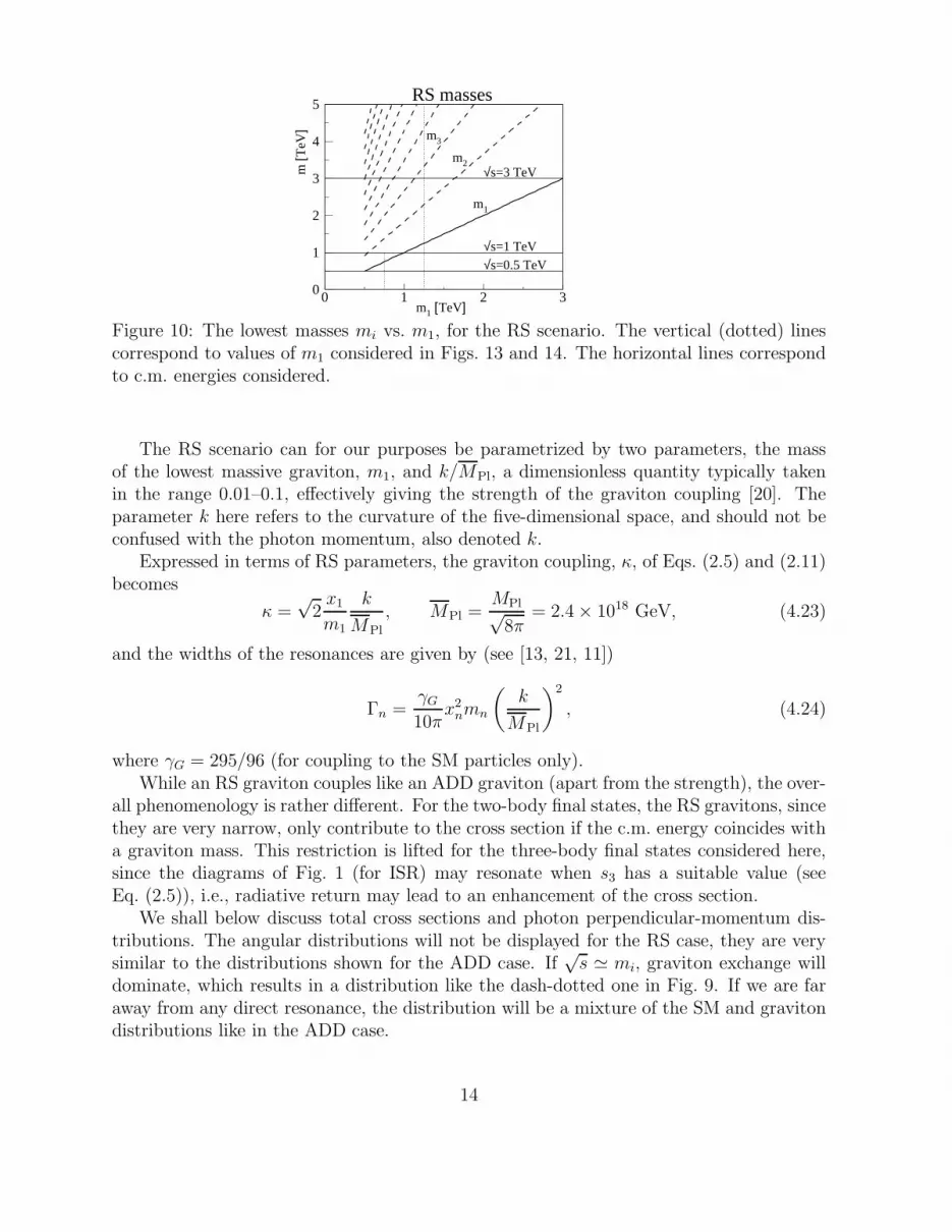
The phenomenology of the RS scenario [6] differs from that of the ADD scenario in sev-eral respects. This scenario has two 3-branes separated in the fifth dimension, and anon-factorisable geometry, which means that the four-dimensional metric depends on thecoordinate in the fifth dimension. It gives rise to a tower of massive KK gravitons with themass of the n’th resonance related to that of the first one, m1, in the following way [20]
mn =xn
x1m1, (4.22)
where xn are zeros of the Bessel function J1(xn) = 0, with x1 ≃ 3.83 (not to be confusedwith the energy fraction carried by the µ−, also denoted x1). Therefore the mass splittingsin the RS model are non-equidistant. The mass of the first resonance is assumed to beof the order of TeV, so only a few resonances are within reach of collider experiments. InFig. 10 we show the lowest states for a range of m1 values. Since there are only a fewgraviton resonances kinematically available, the summation over them is straightforward.
13
0 1 2 30
1
2
3
4
5
m1 [TeV]m
[TeV
]
m1
m2
m3
√s=3 TeV
√s=1 TeV
√s=0.5 TeV
RS masses
Figure 10: The lowest masses mi vs. m1, for the RS scenario. The vertical (dotted) linescorrespond to values of m1 considered in Figs. 13 and 14. The horizontal lines correspondto c.m. energies considered.
The RS scenario can for our purposes be parametrized by two parameters, the massof the lowest massive graviton, m1, and k/MPl, a dimensionless quantity typically takenin the range 0.01–0.1, effectively giving the strength of the graviton coupling [20]. Theparameter k here refers to the curvature of the five-dimensional space, and should not beconfused with the photon momentum, also denoted k.
Expressed in terms of RS parameters, the graviton coupling, κ, of Eqs. (2.5) and (2.11)becomes
κ =√
2x1
m1
k
MPl
, MPl =MPl√
8π= 2.4 × 10¹⁸ GeV, (4.23)
and the widths of the resonances are given by (see [13, 21, 11])
Γn =γG
10πx2
nmn
(
k
MPl
)2
, (4.24)
where γG = 295/96 (for coupling to the SM particles only).While an RS graviton couples like an ADD graviton (apart from the strength), the over-
all phenomenology is rather different. For the two-body final states, the RS gravitons, sincethey are very narrow, only contribute to the cross section if the c.m. energy coincides witha graviton mass. This restriction is lifted for the three-body final states considered here,since the diagrams of Fig. 1 (for ISR) may resonate when s3 has a suitable value (seeEq. (2.5)), i.e., radiative return may lead to an enhancement of the cross section.
We shall below discuss total cross sections and photon perpendicular-momentum dis-tributions. The angular distributions will not be displayed for the RS case, they are verysimilar to the distributions shown for the ADD case. If
√s ≃ mi, graviton exchange will
dominate, which results in a distribution like the dash-dotted one in Fig. 9. If we are faraway from any direct resonance, the distribution will be a mixture of the SM and gravitondistributions like in the ADD case.
14
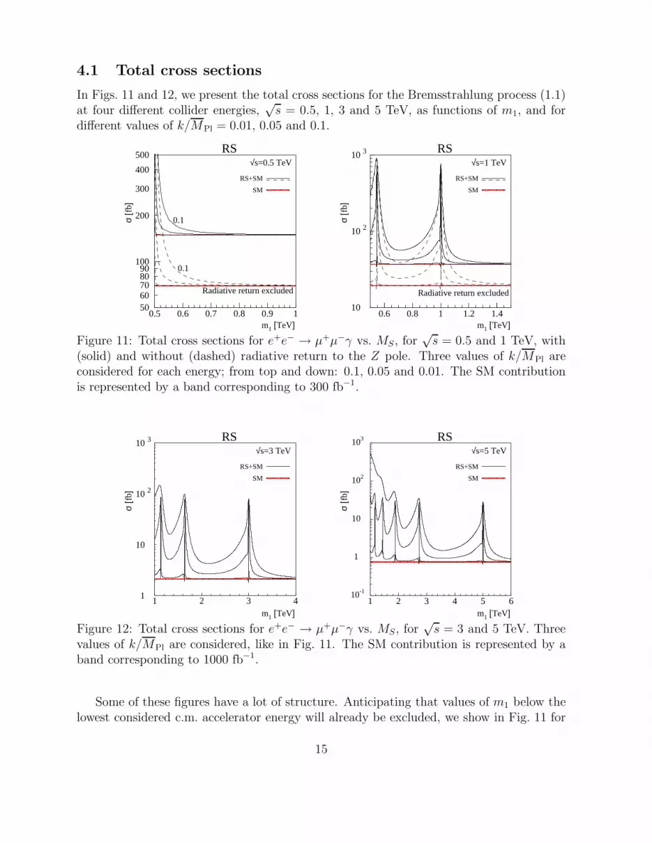
4.1 Total cross sections
In Figs. 11 and 12, we present the total cross sections for the Bremsstrahlung process (1.1)at four different collider energies,
√s = 0.5, 1, 3 and 5 TeV, as functions of m1, and for
different values of k/MPl = 0.01, 0.05 and 0.1.
5060708090
100
200
300
400
500
0.1
0.1
Radiative return excluded
m1 [TeV]
σ [f
b]
RS+SM
SM
0.5 0.6 0.7 0.8 0.9 1
RSs=0.5 TeV√
10
10 2
10 3
Radiative return excluded
m1 [TeV]
σ [f
b]
RS+SM
SM
0.6 0.8 1 1.2 1.4
RSs=1 TeV√
Figure 11: Total cross sections for e+e− → µ+µ−γ vs. MS, for√
s = 0.5 and 1 TeV, with(solid) and without (dashed) radiative return to the Z pole. Three values of k/MPl areconsidered for each energy; from top and down: 0.1, 0.05 and 0.01. The SM contributionis represented by a band corresponding to 300 fb−1.
1
10
10 2
10 3
m1 [TeV]
σ [f
b]
RS+SM
SM
1 2 3 4
RSs=3 TeV√
103
102
10
1
10-1
m1 [TeV]
σ [f
b]
RS+SM
SM
1 2 3 4 5 6
RSs=5 TeV√
Figure 12: Total cross sections for e+e− → µ+µ−γ vs. MS, for√
s = 3 and 5 TeV. Threevalues of k/MPl are considered, like in Fig. 11. The SM contribution is represented by aband corresponding to 1000 fb−1.
Some of these figures have a lot of structure. Anticipating that values of m1 below thelowest considered c.m. accelerator energy will already be excluded, we show in Fig. 11 for
15

√s = 0.5 TeV (left panel) only values of m1 such that m1 >
√s. However, if the resonance
is reasonably broad (high k/MPl), there can be a considerable increase of the cross sectionfor some range of m1 values well above the c.m. energy. Like for the ADD case, exclusionof radiative return to the Z leads to an improvement of the signal.
At the next higher energy studied,√
s = 1 TeV (Fig. 11, right panel), we considera range of m1 values, below the c.m. energy, as well as above. Apart from the obviousresonance peak when m1 ≃
√s, there is also a sharp peak for values of m1 around 0.55 TeV.
From Fig. 10 we see that this corresponds to the second graviton, with mass m2, beingproduced resonantly. We shall refer to both these cases as “direct” resonances, since√
s = mi for some i.In Fig. 12, this phenomenon of producing higher resonances is demonstrated for the
c.m. energies of 3 and 5 TeV. In the right panel of Fig. 12, for√
s = 5 TeV, we see form1 ≃ 1 TeV and large k/MPl an enhancement of the cross section by more than two ordersof magnitude. This is in part caused by the higher resonances being close to each other(and wide), such that several of them can interfere. Also radiative return to lower statescontributes, as discussed below.
In this same panel, we note that there is a significant enhancement of the RS crosssection in the region around m1 = 4 TeV, which is not compatible with any direct resonance(when
√s = 5 TeV). This enhancement is more than what can be attributed to the width
of the nearby resonances, it is caused by diagrams where the s3-channel may resonate, i.e.,where
√s3 ≃ m1 and the remaining energy is carried by the photon.
4.2 Photon perpendicular momentum distributions
In the photon perpendicular-momentum distribution, we expect a harder spectrum thanin the SM case, as was the case for the ADD scenario. Furthermore, resonant productionof either the lowest (m1) or a higher resonance (mi) can lead to a sharp edge for
k⊥ <∼s − m2
i
2√
s, (4.25)
characteristic of radiative return to a lower state, mi <√
s.Fig. 13 is devoted to k⊥ distributions for
√s = 1 TeV, two values of m1, and k/MPl =
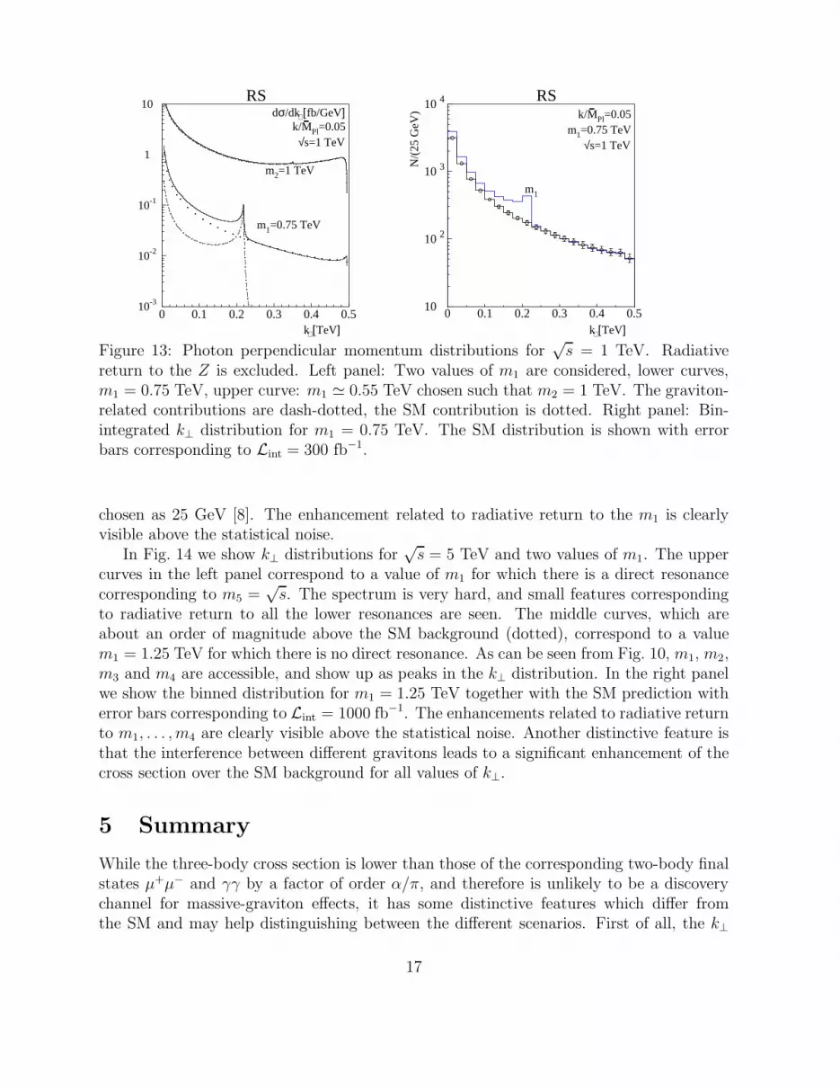
0.05. The higher curves in the left panel show k⊥ distributions for a reasonably low value ofm1, chosen such that the second resonance coincides with the c.m. energy. The distributionis for all k⊥ higher than that of the SM by more than one order of magnitude, the excessincreasing with k⊥. The small structure at k⊥ ∼ 0.35 TeV is due to radiative return tothe lower resonance at m1 ≃ 0.55 TeV, with the “resonant” k⊥ given by Eq. (4.25). Thelower curves in the left panel correspond to a value of m1 = 0.75 TeV for which there is nodirect resonance. Hence, the indirect effect of radiative return becomes more visible, thereis a distinct enhancement at the value of k⊥ corresponding to (4.25).
In the right panel we show the binned distribution for m1 = 0.75 TeV together with theSM prediction with error bars corresponding to Lint = 300 fb−1. The bin width has been
16
10
1
10-1
10-2
10-3
dσ/dk [fb/GeV]⊥
k [TeV]⊥
0 0.1 0.2 0.3 0.4 0.5
RS
k/MPl=0.05
m2=1 TeV
m1=0.75 TeV
s=1 TeV√
-
10
10 2
10 3
10 4
0 0.1 0.2 0.3 0.4 0.5
N/(
25 G
eV)
k [TeV]⊥
RSk/MPl=0.05
m1=0.75 TeV
m1
s=1 TeV√
-
Figure 13: Photon perpendicular momentum distributions for√
s = 1 TeV. Radiativereturn to the Z is excluded. Left panel: Two values of m1 are considered, lower curves,m1 = 0.75 TeV, upper curve: m1 ≃ 0.55 TeV chosen such that m2 = 1 TeV. The graviton-related contributions are dash-dotted, the SM contribution is dotted. Right panel: Bin-integrated k⊥ distribution for m1 = 0.75 TeV. The SM distribution is shown with errorbars corresponding to Lint = 300 fb−1.
chosen as 25 GeV [8]. The enhancement related to radiative return to the m1 is clearlyvisible above the statistical noise.
In Fig. 14 we show k⊥ distributions for√
s = 5 TeV and two values of m1. The uppercurves in the left panel correspond to a value of m1 for which there is a direct resonancecorresponding to m5 =
√s. The spectrum is very hard, and small features corresponding
to radiative return to all the lower resonances are seen. The middle curves, which areabout an order of magnitude above the SM background (dotted), correspond to a valuem1 = 1.25 TeV for which there is no direct resonance. As can be seen from Fig. 10, m1, m2,m3 and m4 are accessible, and show up as peaks in the k⊥ distribution. In the right panelwe show the binned distribution for m1 = 1.25 TeV together with the SM prediction witherror bars corresponding to Lint = 1000 fb−1. The enhancements related to radiative returnto m1, . . . , m4 are clearly visible above the statistical noise. Another distinctive feature isthat the interference between different gravitons leads to a significant enhancement of thecross section over the SM background for all values of k⊥.
5 Summary
While the three-body cross section is lower than those of the corresponding two-body finalstates µ+µ− and γγ by a factor of order α/π, and therefore is unlikely to be a discoverychannel for massive-graviton effects, it has some distinctive features which differ fromthe SM and may help distinguishing between the different scenarios. First of all, the k⊥
17

10-1
10-2
10-3
10-4
dσ/dk [fb/GeV]⊥
k [TeV]⊥
0 0.5 1 1.5 2 2.5
RS
k/MPl=0.05
m5=5 TeV
m1=1.25 TeV
s=5 TeV√
-
1
10
10 2
10 3
10 4
0 0.5 1 1.5 2 2.5
N/(
50 G
eV)
k [TeV]⊥
RSk/MPl=0.05
m1=1.25 TeV
m1m2
m3
m4
s=5 TeV√
-
Figure 14: Photon perpendicular momentum distributions. Radiative return to the Z isexcluded. Left panel: Two values of m1 are considered, lower curves, m1 = 1.25 TeV, uppercurve: m1 ≃ 1.16 TeV is chosen such that m5 = 5 TeV. The graviton-related contributionsare dash-dotted, the SM contribution is dotted. Right panel: Bin-integrated k⊥ distributionfor m1 = 1.25 TeV. The SM distribution is shown with error bars corresponding toLint = 1000 fb−1.
distribution is harder than in the SM. This applies to both the ADD and RS scenarios,and can be particularly important in the RS scenario, if the graviton has a moderatelystrong coupling (determined by k/MPl). Also, the photon angular distribution can have asignificant enhancement at large angles.
In the ADD scenario, where the k⊥ distribution is rather smooth, of the order of oneyear of running would be sufficient to see this hardening of the photon spectrum, for valuesof MS up to about twice the c.m. energy.
In the RS scenario, ISR opens up the possibility of radiative return to the KK gravi-ton resonances within the kinematically accessible range. This can lead to characteristicperpendicular-momentum distributions, and an increase in the cross section even when thec.m. energy is far away from any resonance.
Radiative return to the Z is also possible through ISR, but can be removed by acut. The statistical significance of the signal can improve significantly when such a cut isincluded.
Here we have considered a final state with a lepton pair accompanied by a photon. Itwould also be of interest to consider different final states like qqγ (two jets and a photon)or even gluon Bremsstrahlung, e+e− → qqg (three jets) in future analyses. In the lattercase, the result would however be different from the case considered here (after the trivialsubstitutions for other coupling constants and colour factors). The reason for this differenceis that the gluon can only come from the quark line, the ISR contribution would only yieldphotons, and therefore be of higher order compared to e+e− → three jets.
18
Acknowledgment
This research has been supported in part by the Research Council of Norway.
Appendix A: Angular- and energy-distribution func-
tions
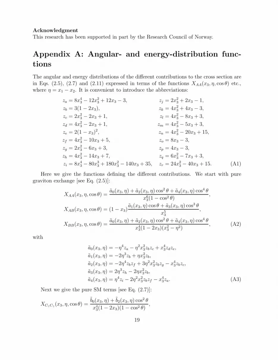
The angular and energy distributions of the different contributions to the cross section arein Eqs. (2.5), (2.7) and (2.11) expressed in terms of the functions XAA(x3, η, cos θ) etc.,where η = x1 − x2. It is convenient to introduce the abbreviations:
za = 8x43 − 12x2
3 + 12x3 − 3, zj = 2x23 + 2x3 − 1,
zb = 3(1 − 2x3), zk = 4x23 + 4x3 − 3,
zc = 2x23 − 2x3 + 1, zl = 4x2
3 − 8x3 + 3,
zd = 4x23 − 2x3 + 1, zm = 4x2
3 − 5x3 + 3,
ze = 2(1 − x3)2, zn = 4x2
3 − 20x3 + 15,
zf = 4x23 − 10x3 + 5, zo = 8x3 − 3,
zg = 2x23 − 6x3 + 3, zp = 4x3 − 3,
zh = 4x23 − 14x3 + 7, zq = 6x2
3 − 7x3 + 3,
zi = 8x43 − 80x3
3 + 180x23 − 140x3 + 35, zr = 24x2
3 − 40x3 + 15. (A1)
Here we give the functions defining the different contributions. We start with puregraviton exchange [see Eq. (2.5)]:
XAA(x3, η, cos θ) =a0(x3, η) + a2(x3, η) cos2 θ + a4(x3, η) cos4 θ
x63(1 − cos2 θ)
,
XAB(x3, η, cos θ) = (1 − x3)a1(x3, η) cos θ + a3(x3, η) cos3 θ
x53
,
XBB(x3, η, cos θ) =a0(x3, η) + a2(x3, η) cos2 θ + a4(x3, η) cos4 θ
x43(1 − 2x3)(x2
3 − η2), (A2)
with
a0(x3, η) = −η4za − η2x23zbzc + x4
3zdze,
a1(x3, η) = −2η3zb + ηx23zb,
a2(x3, η) = −2η4zbzf + 3η2x23zbzg − x4
3zbzc,
a3(x3, η) = 2η3zh − 2ηx23zb,
a4(x3, η) = η4zi − 2η2x23zbzf − x4
3za. (A3)
Next we give the pure SM terms [see Eq. (2.7)]:
XCγCγ (x3, η, cos θ) =b0(x3, η) + b2(x3, η) cos2 θ
x43(1 − 2x3)(1 − cos2 θ)
,
19

XCγCZ(x3, η, cos θ) = XCZCγ (x3, η, cos θ) = vevµXCγCγ + aeaµ
b1(x3, η) cos θ
x43(1 − 2x3)(1 − cos2 θ)
,
XCZCZ(x3, η, cos θ) = (a2
e + v2e)(a
2µ + v2
µ)XCγCγ + 4aeaµvevµb1(x3, η) cos θ
x43(1 − 2x3)(1 − cos2 θ)
,
XCγDγ (x3, η, cos θ) = (1 − x3)η cos θ
x33
,
XCγDZ(x3, η, cos θ) = XCZDγ (x3, η, cos θ) = (1 − x3)
vevµη cos θ − aeaµx3
x33
,
XCZDZ(x3, η, cos θ) = (1 − x3)
(a2e + v2
e)(a2µ + v2
µ)η cos θ − 4aeaµvevµx3
x33
,
XDγDγ (x3, η, cos θ) =b0(x3, η) + b2(x3, η) cos2 θ
x23(x
23 − η2)
,
XDγDZ(x3, η, cos θ) = XDZDγ (x3, η, cos θ) = vevµXDγDγ + aeaµ
b1(x3, η) cos θ
x23(x
23 − η2)
,
XDZDZ(x3, η, cos θ) = (a2
e + v2e)(a
2µ + v2
µ)XDγDγ + 4aeaµvevµb1(x3, η) cos θ
x23(x
23 − η2)
, (A4)
with
b0(x3, η) = η2zj + x23zg,
b1(x3, η) = −4ηx3zc,
b2(x3, η) = η2zg + x23zj . (A5)
Vector and axial couplings are normalized to vf = Tf − 2Qf sin2 θW , af = Tf , with Tf theisospin.
Then we list the graviton-SM interference terms. First we have the pure ISR and FSRterms:
XACγ (x3, η, cos θ) =c1(x3, η) cos θ + c3(x3, η) cos3 θ
x53(1 − cos2 θ)
,
XACZ(x3, η, cos θ) = 2vevµXACγ + aeaµ
c0(x3, η) + c2(x3, η) cos2 θ
x53(1 − cos2 θ)
,
XBDγ (x3, η, cos θ) =c1(x3, η) cos θ + c3(x3, η) cos3 θ
x33(x
23 − η2)
,
XBDZ(x3, η, cos θ) = 2vevµXBDγ + aeaµ
c0(x3, η) + c2(x3, η) cos2 θ
x33(x
23 − η2)
, (A6)
with
c0(x3, η) = −3η2x3zc + x33zc,
c1(x3, η) = η3zb − x23ηzb,
20
c2(x3, η) = 9η2x3zc − 3x33zc,
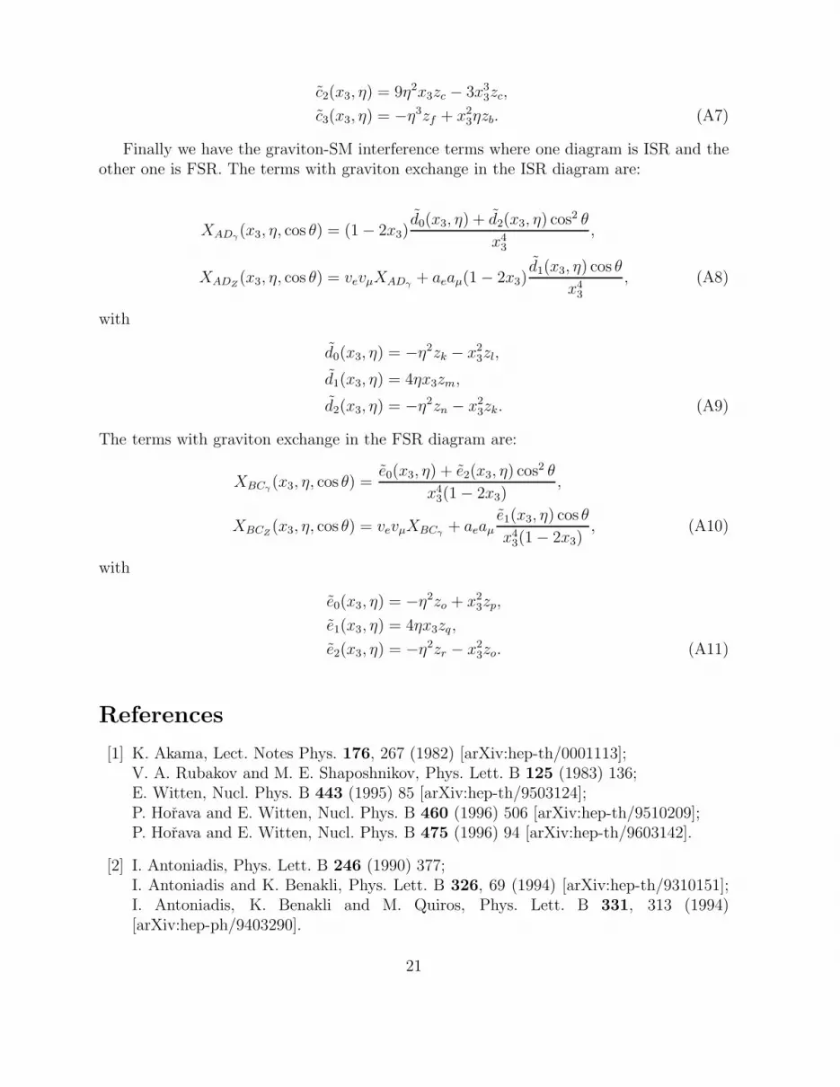
c3(x3, η) = −η3zf + x23ηzb. (A7)
Finally we have the graviton-SM interference terms where one diagram is ISR and theother one is FSR. The terms with graviton exchange in the ISR diagram are:
XADγ(x3, η, cos θ) = (1 − 2x3)d0(x3, η) + d2(x3, η) cos2 θ
x43
,
XADZ(x3, η, cos θ) = vevµXADγ + aeaµ(1 − 2x3)
d1(x3, η) cos θ
x43
, (A8)
with
d0(x3, η) = −η2zk − x23zl,
d1(x3, η) = 4ηx3zm,
d2(x3, η) = −η2zn − x23zk. (A9)
The terms with graviton exchange in the FSR diagram are:
XBCγ (x3, η, cos θ) =e0(x3, η) + e2(x3, η) cos2 θ
x43(1 − 2x3)
,
XBCZ(x3, η, cos θ) = vevµXBCγ + aeaµ
e1(x3, η) cos θ
x43(1 − 2x3)
, (A10)
with
e0(x3, η) = −η2zo + x23zp,
e1(x3, η) = 4ηx3zq,
e2(x3, η) = −η2zr − x23zo. (A11)
References
[1] K. Akama, Lect. Notes Phys. 176, 267 (1982) [arXiv:hep-th/0001113];V. A. Rubakov and M. E. Shaposhnikov, Phys. Lett. B 125 (1983) 136;E. Witten, Nucl. Phys. B 443 (1995) 85 [arXiv:hep-th/9503124];P. Horava and E. Witten, Nucl. Phys. B 460 (1996) 506 [arXiv:hep-th/9510209];P. Horava and E. Witten, Nucl. Phys. B 475 (1996) 94 [arXiv:hep-th/9603142].
[2] I. Antoniadis, Phys. Lett. B 246 (1990) 377;I. Antoniadis and K. Benakli, Phys. Lett. B 326, 69 (1994) [arXiv:hep-th/9310151];I. Antoniadis, K. Benakli and M. Quiros, Phys. Lett. B 331, 313 (1994)[arXiv:hep-ph/9403290].
21

[3] N. Arkani-Hamed, S. Dimopoulos and G. Dvali, Phys. Lett. B 429 (1998) 263[arXiv:hep-ph/9803315].
[4] K. R. Dienes, E. Dudas and T. Gherghetta, Phys. Lett. B 436, 55 (1998)[arXiv:hep-ph/9803466].
[5] N. Arkani-Hamed, S. Dimopoulos and G. Dvali, Phys. Rev. D 59 (1999) 086004[arXiv:hep-ph/9807344].
[6] L. Randall and R. Sundrum, Phys. Rev. Lett. 83 (1999) 3370 [arXiv:hep-ph/9905221].
[7] L. Randall and R. Sundrum, Phys. Rev. Lett. 83 (1999) 4690 [arXiv:hep-th/9906064].
[8] J. A. Aguilar-Saavedra et al. [ECFA/DESY LC Physics Working Group Collabora-tion], “TESLA Technical Design Report Part III: Physics at an e+e- Linear Collider,”DESY-01-011, arXiv:hep-ph/0106315;T. Abe et al. [American Linear Collider Working Group Collaboration], “Linear col-lider physics resource book for Snowmass 2001. 1: Introduction,” in Proc. of theAPS/DPF/DPB Summer Study on the Future of Particle Physics (Snowmass 2001)ed. N. Graf, SLAC-R-570, arXiv:hep-ex/0106055.
[9] R. W. Assmann et al., “A 3-TeV e+ e- linear collider based on CLIC technology,”SLAC-REPRINT-2000-096.
[10] F. A. Berends and R. Kleiss, Nucl. Phys. B 177, 237 (1981);F. A. Berends, R. Kleiss and S. Jadach, Nucl. Phys. B 202, 63 (1982).
[11] E. Dvergsnes, P. Osland and N. Ozturk, Phys. Rev. D 67, 074003 (2003)[arXiv:hep-ph/0207221]; E. Dvergsnes, P. Osland and N. Ozturk, in Proceedings of16th International Workshop on High Energy Physics and Quantum Field Theory(QFTHEP 2001), edited by M.N. Dubinin and V.I. Savrin, Moscow, Russia, Skobelt-syn Inst. Nucl. Phys., 2001, pp. 54-63, arXiv:hep-ph/0108029.
[12] K. m. Cheung and G. Landsberg, Phys. Rev. D 62, 076003 (2000)[arXiv:hep-ph/9909218].
[13] T. Han, J. D. Lykken and R. Zhang, Phys. Rev. D 59 (1999) 105006[arXiv:hep-ph/9811350].
[14] R. Contino, L. Pilo, R. Rattazzi and A. Strumia, JHEP 0106, 005 (2001)[arXiv:hep-ph/0103104].
[15] G. F. Giudice, R. Rattazzi and J. D. Wells, Nucl. Phys. B 544 (1999) 3[arXiv:hep-ph/9811291].
[16] J. L. Hewett, Phys. Rev. Lett. 82 (1999) 4765 [arXiv:hep-ph/9811356].
22
[17] S. Hannestad and G. Raffelt, Phys. Rev. Lett. 87, 051301 (2001) [hep-ph/0103201];S. Hannestad and G. G. Raffelt, Phys. Rev. Lett. 88, 071301 (2002) [hep-ph/0110067].
[18] T. G. Rizzo, JHEP 0210 (2002) 013 [arXiv:hep-ph/0208027]; JHEP 0302, 008 (2003)[arXiv:hep-ph/0211374].
[19] P. Osland, A. A. Pankov and N. Paver, Phys. Rev. D 68, 015007 (2003)[arXiv:hep-ph/0304123].
[20] H. Davoudiasl, J. L. Hewett and T. G. Rizzo, Phys. Rev. Lett. 84 (2000) 2080[arXiv:hep-ph/9909255]; Phys. Rev. D 63 (2001) 075004 [arXiv:hep-ph/0006041].
[21] B. C. Allanach, K. Odagiri, M. A. Parker and B. R. Webber, JHEP 0009, 019 (2000)[arXiv:hep-ph/0006114].
23