Global structure of periodicity hubs in Lyapunov

phase diagrams of dissipative flows

Renato Vitolo, Paul Glendinning and Jason A.C. Gallas

July 2011

MIMS EPrint: 2011.57

Manchester Institute for Mathematical Sciences

School of Mathematics

The University of Manchester

Reports available from: http://www.manchester.ac.uk/mims/eprints

And by contacting: The MIMS Secretary

School of Mathematics

The University of Manchester

Manchester, M13 9PL, UK

ISSN 1749-9097

Global structure of periodicity hubs in Lyapunov phase diagrams of dissipative flows

Renato Vitolo,1 Paul Glendinning,2 and Jason A.C. Gallas1, 3, 4

1School of Engineering, Computing and Mathematics, University of Exeter, Exeter EX4 4QF, UK2School of Mathematics, University of Manchester, Oxford Road, Manchester M13 9PL, UK3Departamento de Fısica, Universidade Federal da Paraıba, 58051-970 Joao Pessoa, Brazil

4Institute for Multiscale Simulation, Friedrich-Alexander Universitat, 91052 Erlangen, Germany(Dated: 29 de Maio de 2011, as 20:35)

Infinite cascades of periodicity hubs were predicted and very recently observed experimentallyto organize stable oscillations of some dissipative flows. Here we describe the global mechanismunderlying the genesis and organization of networks of periodicity hubs in control parameter spaceof a simple prototypical flow. We show that spirals associated with periodicity hubs emerge/accu-mulate at the folding of certain fractal-like sheaves of Shilnikov homoclinic bifurcations of a commonsaddle-focus equilibrium. The specific organization of hub networks is found to depend strongly onthe interaction between the homoclinic orbits and the global structure of the underlying attractor.

I. INTRODUCTION

To study the response of a system with respect tochanges in the processes involved is a basic problem inphysics and the quantitative sciences in general. For dis-sipative systems, the problem is formulated in terms ofthe attractors typically underlying the long-term dynam-ical behavior, see e.g. [1, 2]. Here one aims to understandthe transitions (bifurcations) of the attractors under vari-ation of the system’s control parameters.

Numerical computation of Lyapunov exponents pro-vides a convenient tool to classify attractors and bifurca-tions of dynamical systems. A positive or zero maximalLyapunov exponent usually indicates sensitivity with re-spect to the initial conditions or, respectively, temporallyregular behavior (e.g. periodic or quasi-periodic) [1, 2].With the development of fast throughput numerical ex-periments, it becomes feasible to explore large ranges ofparameter space, classifying the system’s attractors bytheir Lyapunov exponents. Lyapunov phase diagrams aregraphical summaries of these explorations, describing theattractor type as a function of the control parametersthrough color or gray scale codes. Such diagrams havebeen obtained both numerically [3–16] and experimen-tally [17] and may offer a wealth of information on thethe nature of the attractors and their bifurcations. Lya-punov phase diagrams are useful since they code only thestable dynamics and, hence, the dynamics which is likelyto be observable and relevant in any physical system.

A specific class of spiral-like structures has been iden-tified in Lyapunov phase diagrams of dissipative flows asdiverse as piecewise-linear resistive electric circuits, elec-trical circuits with smooth nonlinearities, certain lasers,chemical oscillators and other paradigmatic flows [3–7, 15, 16]. These structures consist of a double alterna-tion of nested spirals converging to a central point: theso-called periodicity hub. Fig. 1 shows a periodicity hubin the (c, a)-parameter plane of Rossler’s oscillator [18]:

x = −y − z, y = x + ay, z = (b + z)x− cz, (1)

where b = 0.3. Two groups of nested spiral-shaped re-

4.0 6.0c

0.3

0.4

a

-2.02 0.240

4.0 6.0c

0.3

0.4

a

h1

H1

H13

H12

H11

FIG. 1. (Color online) Lyapunov phase diagram for Rossler’soscillator, with four dots marking periodicity hubs H1 andH1j , j = 1, 2, 3 and with a curve h1 of Shilnikov homoclinicbifurcations. Grey tones, identifying the periodicity spirals,are proportional to the maximum nonzero Lyapunov expo-nent. Color, identifying the chaoticity spiral, depends on themaximum Lyapunov exponent, which is positive. The dia-gram displays 24002 = 5.76 × 106 parameter points.

gions accumulate in the parameter plane around the pe-riodicity hub H1: periodicity and chaoticity spirals. In-dividual periodicity (chaoticity) spirals are characterizedby a zero (positive) maximum Lyapunov exponent, corre-sponding to periodic (chaotic) stable oscillations in phasespace. Both groups seems to contain infinitely many spi-rals. As parameters approach H1 within a single period-

2

1.0 10.0c

0.2

0.53

a

(a)

H

H

1

2

3.0 5.0c

0.41

0.53

a

h h h h h5 4 3 2 1

H

H

3

2

(b)

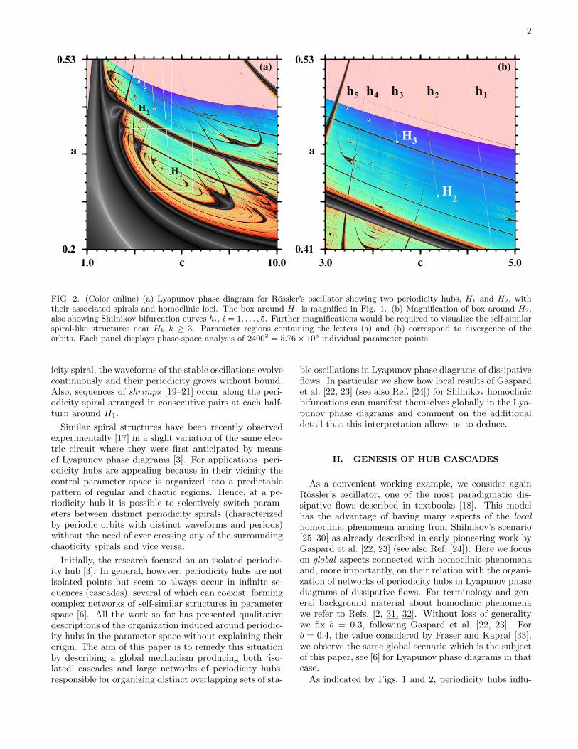
FIG. 2. (Color online) (a) Lyapunov phase diagram for Rossler’s oscillator showing two periodicity hubs, H1 and H2, withtheir associated spirals and homoclinic loci. The box around H1 is magnified in Fig. 1. (b) Magnification of box around H2,also showing Shilnikov bifurcation curves hi, i = 1, . . . , 5. Further magnifications would be required to visualize the self-similarspiral-like structures near Hk, k ≥ 3. Parameter regions containing the letters (a) and (b) correspond to divergence of theorbits. Each panel displays phase-space analysis of 24002 = 5.76 × 106 individual parameter points.

icity spiral, the waveforms of the stable oscillations evolvecontinuously and their periodicity grows without bound.Also, sequences of shrimps [19–21] occur along the peri-odicity spiral arranged in consecutive pairs at each half-turn around H1.

Similar spiral structures have been recently observedexperimentally [17] in a slight variation of the same elec-tric circuit where they were first anticipated by meansof Lyapunov phase diagrams [3]. For applications, peri-odicity hubs are appealing because in their vicinity thecontrol parameter space is organized into a predictablepattern of regular and chaotic regions. Hence, at a pe-riodicity hub it is possible to selectively switch param-eters between distinct periodicity spirals (characterizedby periodic orbits with distinct waveforms and periods)without the need of ever crossing any of the surroundingchaoticity spirals and vice versa.

Initially, the research focused on an isolated periodic-ity hub [3]. In general, however, periodicity hubs are notisolated points but seem to always occur in infinite se-quences (cascades), several of which can coexist, formingcomplex networks of self-similar structures in parameterspace [6]. All the work so far has presented qualitativedescriptions of the organization induced around periodic-ity hubs in the parameter space without explaining theirorigin. The aim of this paper is to remedy this situationby describing a global mechanism producing both ‘iso-lated’ cascades and large networks of periodicity hubs,responsible for organizing distinct overlapping sets of sta-

ble oscillations in Lyapunov phase diagrams of dissipativeflows. In particular we show how local results of Gaspardet al. [22, 23] (see also Ref. [24]) for Shilnikov homoclinicbifurcations can manifest themselves globally in the Lya-punov phase diagrams and comment on the additionaldetail that this interpretation allows us to deduce.

II. GENESIS OF HUB CASCADES

As a convenient working example, we consider againRossler’s oscillator, one of the most paradigmatic dis-sipative flows described in textbooks [18]. This modelhas the advantage of having many aspects of the localhomoclinic phenomena arising from Shilnikov’s scenario[25–30] as already described in early pioneering work byGaspard et al. [22, 23] (see also Ref. [24]). Here we focuson global aspects connected with homoclinic phenomenaand, more importantly, on their relation with the organi-zation of networks of periodicity hubs in Lyapunov phasediagrams of dissipative flows. For terminology and gen-eral background material about homoclinic phenomenawe refer to Refs. [2, 31, 32]. Without loss of generalitywe fix b = 0.3, following Gaspard et al. [22, 23]. Forb = 0.4, the value considered by Fraser and Kapral [33],we observe the same global scenario which is the subjectof this paper, see [6] for Lyapunov phase diagrams in thatcase.

As indicated by Figs. 1 and 2, periodicity hubs influ-

3

-1 0 1 2

0 1 2 3 4

(c)

xy

Ws(O)

-1 0 1 2

(b)

xy

Wu(O)

-1 0 1 2

(a)

xyF1

y

(d)

F1~ 10

-10

y

(e) h1,+

Wu(O)

y

(f)

h1,-

y

x

(g)

Ws(O)

FIG. 3. (Color online) Illustration of homoclinic bifurcationsin Rossler’s oscillator. Left column: primary intersections ofthe manifolds W s(O) (dot) and Wu(O) (curve) with the planeΣ for a = 0.35 fixed and: (a) c = 5.2, (b) c = 4.88722732, (c)c = 4.6, showing the transit of W s(O) across Wu(O) whenthe parameter c is changed. Right column: sketches magni-fying the folding region F1 of the unstable manifold Wu(O).(d) and (g): sketches of (a) and (c), respectively. What lookslike a single curve in the left column panels is a pair of curves,which are narrowly spaced due to strong compression in thenormal direction. Two distinct homoclinic bifurcations h1,+

and h1,− take place for nearby parameter values, due to thefolding and compression (panels (e,f)). These two configura-tions cannot be distinguished from each other at the scale ofpanel (b).

ence extended portions of the parameter space. Figure1 suggests that an infinite sequence of periodicity hubsH1j converges to H1: most of the periodicity spirals at-tached to the H1j can only be seen in magnifications ofthe Lyapunov phase diagram. However, a few shrimpsalong these periodicity spirals are visible at the scale ofFig. 1, where they are highlighted by circles. Additionalhubs Hk are revealed by examining a larger parameterdomain (see Fig. 2(a)). The infinite alternation of spiralsnear H2 is shown magnified in Fig. 2(b). By special-ized numerical methods [32], we find several loci hk ofShilnikov homoclinic bifurcations [22–24] which, at thescale of Fig. 2 (b), seem to terminate at each hub Hk, fork = 1, . . . , 5.

We now address the fundamental question of this pa-per: what is the mechanism responsible for generatinghubs and hub networks in Lyapunov phase diagrams andwhat is its relation with Shilnikov homoclinic bifurca-tions? A key concept here is that the hub network seenin parameter space is intimately related to the interac-tion in phase-space between the homoclinic orbits andthe global structure of the Rossler attractor. Hence thediscussion will now be focused on the structures in phasespace.

To see how hub networks arise, we consider a sub-set of Rossler’s (a, c)-parameter plane where the originO ≡ (0, 0, 0) is a saddle focus with a 1D stable manifold

-4

0

4

8

-8-4 0 4

0

5

10

15

20

25(a)z

x

y-4

0

4

8

-8-4 0 4

0

5

10

15

20

25(b)z

x

y

FIG. 4. (Color online) Homoclinic orbits in Rossler’s oscil-lator, for parameter values at the periodicity hubs H1 andH2 as in Fig. 1. (a) A segment of W s(O) (green, solid)connects to an orbit segment in Wu(O) (red, dashed) at apoint on Σ (green dot), for (c, a) = (4.93029864, 0.3301), cor-responding to H1. (b) A primary intersection point of Wu(O)with Σ (blue triangle) is mapped to the primary intersectionpoint of W s(O) with Σ (green dot) by the Poincare map, for(c, a) = (4.18195201, 0.4436), corresponding to H2.

W s(O) and a 2D unstable manifold Wu(O), see e.g. [22,Figure 1]. In this setting, the structure of the Rosslerstrange attractor is essentially determined by the geome-try of Wu(O). This geometry is analyzed as usual [2], ina Poincare section of Wu(O) by a surface Σ, taken hereas the plane z = 3:

Σ = {(x, y, z) ∈ R3 | z = 3}. (2)

As usual [2, 31, 32], we examine the primary intersec-tions of W s(O) and Wu(O) with Σ: loosely speaking,these consist of the points where orbits starting in thecorresponding local manifolds hit Σ for the first time [35].

The left column of Fig. 3 illustrates the process gen-erating a homoclinic bifurcation, seen from within thePoincare section Σ. The figure shows sections of the sta-ble and unstable manifolds of the origin for three valuesof the parameter c, with a fixed. For c = 5.2 and c = 4.6,the stable manifold WS(O) lies at different sides with re-spect to Wu(O). The intermediate value of c is chosensuch that W s(O) actually enters Wu(O): this conditionidentifies a single point in the parameter plane for whicha homoclinic bifurcation occur. Loosely speaking, to de-crease the parameter c with constant a is equivalent tomove W s(O) across Wu(O). Figure 4 shows the homo-clinic orbits occurring for parameter values (c, a) at H1

and H2 in Fig. 1.The manifold Wu(O) has a region of strong curvature

where it folds onto itself. This region, labeled by F1 inFig. 3, is very hard to visualize in the original (x, y) co-ordinates of Σ. This is due to strong compression in thenormal direction to the unstable manifold Wu(O), whichin turn is due to the dissipativity of the system. To visu-

4

(A)

a

c

(A)

a

c

(A)

a

c

(A)

a

c

(A)

a

c

h11 H11

h12 H12

h13H13

H1h1

<10-8

(B)

x

y

F1

F11

F12

(B)

x

y

F1

F11

F12

(B)

x

y

F1

F11

F12

(B)

x

y

F1

F11

F12

(B)

x

y

F1

F11

F12

(B)

x

y

F1

F11

F12

(B)

x

y

F1

F11

F12

(B)

x

y

F1

F11

F12

(B)

x

y

F1

F11

F12

(B)

x

y

F1

F11

F12

(B)

x

y

F1

F11

F12

FIG. 5. (Color online) (A) Parameter plane sketch of thehomoclinic loci h1, h11, h12, h13 (green, solid lines) with fold-ing points at the hubs H1, H11, H12, H13. (B) Sketch withinthe Poincare section Σ of the primary (red, solid line) andsecondary (green, dashed line) intersection of Wu(O) with Σ,see [35], highlighting regions with strong curvature of Wu(O),namely F1 for the primary intersection and F11, F12 for thesecondary intersection. Such regions of folding of the unstablemanifold correspond to the hubs H1, H11, F12 in panel (A).

alize the folding region we resort to hand-made sketchesin the right panels of Fig. 3. The sketches clarify thata pair of homoclinic bifurcations h1,+ and h1,− actuallytakes place near the folding region F1. Since the widthof the folding region is about 10−10, the two homoclinicbifurcations occur for values of the parameter c which arevery close to each other.

Having described how the homoclinic bifurcations oc-cur for a fixed value of a, we now vary both parameters(c, a) in order to locate the homoclinic loci hi in the pa-rameter plane. These loci are obtained by tuning pa-rameters so that W s(O) (the dot in the left column ofFig. 3) lies along Wu(O) (the curve). We refer again tothe sketches in the right column of Fig. 3: to decreasea corresponds to shifting the pair of points h1,± towardsthe left (decreasing x). Hence, a pair of homoclinic bi-furcation curves will occur in the parameter plane.

Again we see here the idea that structures in phasespace have a close correspondence with structures in theparameter plane: the folding region of the unstable man-ifold Wu(O) corresponds to a folding region for the ho-moclinic locus h1 in Fig. 1. Hence, locus h1 actuallyconsists of a pair of narrowly spaced bifurcation curves,to which bifurcation points h1,+ and h1,− of Fig. 3 (e,f)respectively belong. This pair of curves cannot be re-solved at the scale of Fig. 1: as for Fig. 3, we must turnto a sketch in Fig. 5 (a) to illustrate the configuration ofh1. We now see that the periodicity hub H1 occurs atthe folding region of h1 in Fig. 1.

It is worth to emphasize that, for a concrete system,the periodicity hub H1 is not a single point in parameterspace, rather a small region of strong curvature of thehomoclinic locus h1. Indeed, a single point is obtainedonly in the limit of infinite contraction for a local return

map near the homoclinic orbit, see [23, Sec. 4]. However,contraction (due to dissipation) is usually so large thatthat periodicity hubs can be regarded as points for allpractical purposes in many systems encountered in theapplications.

Local analysis near the homoclinic orbit at the foldingpoints reveals the basic structure of the periodicity spiralsin a neighborhood of the hubs [23]. The standard theoryof simple Shilnikov homoclinic bifurcations without fold-ing points [24] shows that there is an infinite sequenceof subsidiary homoclinic orbits accumulating on a prin-cipal homoclinic orbit. This yields an accumulation ofhomoclinic loci in parameter space from one side of theprincipal homoclinic locus. This theory can be adaptedto the folding points to show that an infinite sequenceof subsidiary folding points accumulates on a principalfolding point with a geometrical rate. The position of thesubsidiary foldings relative to the principal folding (i.e.outside or inside the principal folding point) depends onthe sign of two normal form coefficients [36].

For the Rossler system (1), we find the subsidiary fold-ing points to lie inside the principal folding at F1, seeFig. 5 (b). The fourth largest periodicity hub H11 inFig. 1 is generated by a similar mechanism as H1, withthe difference that a subsidiary branch of Wu(O) is in-volved – namely that giving rise to F11 in Fig. 5 (b) – in-stead of the principal branch of Fig. 4 (a), involved in H1.Accordingly, H11 is the folding region of a homoclinic lo-cus h11, which is nested within the principal folded locush1. Analogous considerations imply that folded homo-clinic loci h1j emerge from hubs H1j , j = 2, 3, . . . and arenested into one another, see the sketch in Fig. 5 (a). Thewhole process repeats ad infinitum: Subsidiaries withinsubsidiaries will also show up nearby, giving rise to asheaf of homoclinic loci nested within h1 in Fig. 1. Thissheaf is tightly packed, due to contraction in phase space:the distance between the two branches of h1 is less than10−8, see the sketch in Fig. 5 (a).

A very similar bifurcation structure was analyzed indetail by de Feo et al. [15, 16] for the Colpitts oscillator,by means of both numerical continuation of bifurcationsof periodic orbits and direct integration. Our analysis inthe next section, however, clarifies the link between themulti-branch structure of the attractor and the globalorganization of the hub network. We also link the normalform coefficients of the return map to the position ofthe subsidiary folding points [36]. More importantly, thearrangement reported in our Fig. 5 is quite different fromwhat is described in Fig. 13 of de Feo et al. [15].

III. LYAPUNOV PHASE DIAGRAMS ANDHOMOCLINIC LOCI

So what can we learn from the Lyapunov phase dia-gram? Is it possible to somehow guess the location ofhomoclinic loci from Lyapunov phase diagrams? Beforeproceeding, we invite the reader to try to use the knowl-

5

0.55 1.05α0.36

0.53

β

-2.37 0.140

0.55 1.05α0.36

0.53

β

(a)

1.0 13.0γ

0.25

0.41

δ

-2.75 0.360

1.0 13.0γ

0.25

0.41

δ

(b)

FIG. 6. (Color online) Two additional examples to illustrate the genericity of the global structure of hub networks. (a) hubnetwork for a chemical oscillator [6, 22]. (b) hub network in a simple electronic circuit with a tunnel diode [7]. White boxesmark the location of the two largest hub networks, many more exist. Lyapunov phase diagrams provide a quick guide aboutwhere to find homoclinic loci in control space of flows. Panels display 24002 = 5.76 × 106 parameter points.

edge won by reading the previous Section to guess wherehomoclinic loci are to be expect in the pair of Lyapunovphase diagrams shown in Fig. 6.

With hindsight, without resorting to computation ofhomoclinic bifurcations, the diagrams indeed show clear-cut signatures which allow us to deduce the existence ofhomoclinic loci and locate their folding points. For ex-ample, the detection of the hub H2 (Fig. 2) led us totry to explain this as part of the evolution of the Rosslerattractor when changing parameters. The result of thisinvestigation is shown in Fig. 7. Depending on the pa-rameters, the intersection of the Rossler attractor (or,equivalently, of Wu(O)) with an appropriately chosen re-turn plane develops well-separated bands. Each band hasa fractal onion-like structure arising from the expanding,folding and return of the manifold Wu(O) to the Poincaresection Σ. Also, each band has a point Fj of strong cur-vature, where Wu(O) is folded onto itself, just like F1 inFig. 3. According to Ref. [23], each folding contributesone periodicity hub through the mechanism illustratedin Figs. 3 and 5. Again, periodicity hubs centered atH2 and H3 in parameter plane (Fig. 2(b)) are inducedby folding regions F2 and F3 of the unstable manifoldin phase space (Fig. 7). Each periodicity hub Hk is thefolding point of a homoclinic locus hk, with an associ-ated sequence of subsidiary homoclinic loci hkj and theirfolding points Hkj . Since homoclinic loci have an infinitenumber of subsidiaries, we see nothing preventing theexistence of an infinite number of such new independenthubs, as anticipated by numerical simulations [6].

-7

-5

-3

-1

1 (a)

xy

F1

(b)

xy

F2

-7

-5

-3

-1

1

0 1 2 3

(c)

x

y

F3

0 1 2 3

(d)

x

y

F5

F4

FIG. 7. (Color online) Intersection of Wu(O) with the planeΣ for c = 4 and: (a) a = 0.4, (b) a = 0.46, (c) a = 0.475, (d)a = 0.485. Folding of Wu(O) occurs near each Fj , comparewith Fig. 3. Periodicity hubs arise at such foldings of themanifold, thus giving origin to an infinite network of hubs incontrol parameter space.

We emphasize that the existence of the extra foldingpoints Fj , with j > 1 is a novel and general feature thatdepends on specific details of the attractor of the systembeing considered: it does not follow from the local un-folding of a higher codimension bifurcation point in anyobvious way (although there may still be a relationshipwith mixed-mode oscillation theory [37], see for exam-

6

ple [38]). Correspondingly, the homoclinic orbits at thevarious hubs have a rather different structure (Fig. 4).

Seen in this light, periodicity hubs become a usefultool for the quick detection and understanding of globalfeatures of the parameter space. Features such as homo-clinic folding points and their subsidiary bifurcations arenormally only found by using specialized numerical meth-ods, whilst a theoretical understanding of the Lyapunovphase diagrams allows the existence of these features tobe deduced from the structure of the diagram itself.

The mechanism described here for the occurrence ofperiodicity hub networks involves Shilnikov homoclinicbifurcations. The latter are codimension-one phenom-ena, meaning that they are stably observed in systemsdepending on one parameter [2]. In the present scenario,individual cascades of periodicity hubs require at leasttwo parameters, since a region of strong curvature is alsoneeded along a curve of Shilnikov bifurcations. Hence,periodicity hubs can be considered as codimension-twophenomena, to be expected in systems with Shilnikov bi-furcations when at least two parameters are varied. Tech-nically speaking, a codimension-two condition is only ob-tained in the idealized situation of infinite contractiondiscussed above, see [23, Sec. 4].

Hub networks are indeed found in several physicalmodels [6]: Fig. 6 shows Lyapunov phase diagrams for achemical oscillator first introduced and analyzed by Gas-pard et al. [6, 23] and for a circuit containing a tunneldiode [7], illustrating the similarity with the hub struc-ture in Fig. 1. Hitherto, most work has concentratedon describing the features of the parameter space nearthe periodicity hubs found in these diagrams. Here wehave complemented such understanding by showing howperiodicity hubs are globally related to folding points ofhomoclinic loci described locally in Ref. [23], and haveexplained further properties of hubs close to a principalhub in terms of homoclinic bifurcation theory.

IV. CONCLUSIONS AND OUTLOOK

In this paper we have described the global mechanismunderlying the genesis and organization of networks ofperiodicity hubs in the control parameter space of a sim-ple prototypical flow. We have clarified the relation be-tween periodicity hubs and the presence of two distincttypes of spiral-like regions, respectively characterized byfamilies of periodic or chaotic oscillations. The link ismade clear by Lyapunov phase diagrams, which give afairly complete view of the dynamics and show the keyrole of periodicity hubs in organizing extended portionsof the parameter space. Periodicity and chaoticity spi-rals in the parameter plane emerge from and accumu-late at periodicity hubs: these are small regions of strongcurvature of homoclinic bifurcation curves of a commonsaddle-focus equilibrium. These homoclinic bifurcationcurves are arranged in fractal-like sheaves in the param-eter plane.

The specific organization of hub networks was shownto depend strongly on the interaction between the ho-moclinic orbits and the global structure of the underly-ing attractor. Based on considerations of genericity indynamical systems [2, 31], we argued that the mecha-nism described here, responsible for hub networks, mightbe found in a wide class of dissipative flows, namely asubset of those where Shilnikov’s homoclinic scenario oc-curs [2, 18, 22–31]. At the same time, we do not excludethe possibility that periodicity hubs occur in systemswith other non-Shilnikov reinjection mechanisms, seee.g. [5]. Furthermore, there exist examples of Shilnikov’sscenario in the literature, without detectable periodicityhubs.

Lyapunov phase diagrams are efficient and useful ex-ploratory tools for applications, to understand global fea-tures of complex attractors. For Rossler’s system, thehomoclinic locus h2 was first computed using specializednumerical methods to detect homoclinic phenomena [22].However, the existence of h2 and the several additionalhomoclinic loci hk with folding points has been read offhere directly from Lyapunov phase diagram like Fig. 2,a fact that greatly simplified their precise numerical cal-culation. This led to the discovery of the global bandedstructure of Rossler’s attractor (Fig. 7) and of the addi-tional hubs related to this structure. We believe that theuse of Lyapunov phase diagrams can significantly aug-ment and speed-up the understanding of physical mod-els: such diagrams, focused on experimentally measur-able features, reveal the occurrence of many global bifur-cations without recourse to more specialized numericaltechniques. They are therefore a very powerful way tobegin the analysis of nonlinear systems and can also beapplied to laboratory experiments which, of course, onlydetect stable structures. A complementary tool that maybe useful in analyzing dynamical systems is the directstudy of the oscillations as parameters are tuned [37].

In conclusion, although our emphasis here was onShilnikov’s homoclinic scenario, periodicity hubs havebeen reported very recently for a semiconductor laserwith optoelectronic feedback [5], which is an excitablesystem with multiple time-scale dynamics [39, 40]. As an-ticipated theoretically by Marino et al. [39], such consid-erably richer scenarios are possible in higher-dimensionalsystems, particularly when period-doubling cascades fol-low a Hopf bifurcation and subsequent canard explosion,producing alternations of periodic and chaotic oscilla-tions. As the amplitude of the chaotic attractors growsone observes a spiking regime consisting of large pulsesseparated by irregular time intervals in which the systemdisplays small-amplitude chaotic oscillations. This sce-nario, reminiscent of Shilnikovs homoclinic chaos despitethe fact that no homoclinic connections are involved, hasalready been observed very recently in ground-breakingexperimental studies of a semiconductor laser [41, 42].An interesting challenge now is to uncover the mecha-nism generating networks of hubs for such non-Shilnikovsystems [5].

7

RV acknowledges support by the Willis Research Net-work. (www.willisresearchnetwork.com). JACG thanksthe Royal Society for a fruitful month spent in Exeter,

in June 2009. He also thanks support from the AFOSRGrant FA9550-07-1-0102, and CNPq, Brazil. Bitmapswere computed in the CESUP-UFRGS clusters.

[1] Y.C. Lai and T. Tel, Transient Chaos, (Springer, NewYork, 2011).

[2] P. Glendinning, Stability, Instability and Chaos, (Cam-bridge University Press, Cambridge, 1994).

[3] C. Bonatto and J.A.C. Gallas, Phys. Rev. Lett. 101,054101 (2008).

[4] G.M. Ramırez-Avila and J.A.C Gallas, Revista Bolivianade Fisica 14, 1-9 (2008); Phys. Lett. A 375, 143 (2010).

[5] J.G. Freire and J.A.C. Gallas, Phys. Rev. E 82, 037202(2010).

[6] J.A.C. Gallas, Int. J. Bif. Chaos 20, 197 (2010).[7] R.E. Francke and J.A.C. Gallas, Observation of spirals

and infinite hub hierarchies in self-excited oscillations ofa tunnel diode, preprint, 2011.

[8] H.W. Broer, C. Simo and R. Vitolo, Phys. D 237(13),1773 (2008).

[9] R. Vitolo, C. Simo and H.W. Broer, Nonlinearity, 23,1919 (2010).

[10] H.W. Broer, C. Simo and R. Vitolo, Discrete Contin.Dyn. Syst. B, 14(3) 871 (2010).

[11] A.E. Sterk, R. Vitolo, H.W. Broer, C. Simo, and H. Di-jkstra. Phys. D, 239(10) 702 (2010).

[12] R. Vitolo, C. Simo and H.W. Broer, Regul. Chaotic Dyn.16(1-2), 154 (2011).

[13] V. Kovanis, A. Gavrielides, and J.A.C. Gallas, Eur. Phys.J. D 58, 181 (2010).

[14] A. Celestino, C. Manchein, H.A. Albuquerque, and M.W.Beims, Phys. Rev. Lett. 106, xxx (2011), in print.

[15] O. de Feo, G.M. Maggio, and M.P. Kennedy, Int. J. Bif.Chaos 10, 935 (2000).

[16] O. de Feo and G.M. Maggio, Int. J. Bif. Chaos 13, 2917(2003).

[17] R. Stoop, P. Benner, and Y. Uwate, Phys Rev. Lett. 105,074102 (2010).

[18] O.E. Rossler, Ann. N.Y. Acad. Sci. 316, 376 (1979).[19] Shrimps are formed by a regular set of adjacent windows

centered around a main pair of intersecting superstableparabolic arcs. A shrimp is a doubly infinite mosaic ofstability domains composed by an innermost main do-main plus all the adjacent stability domains arising fromtwo period-doubling cascades together with their corre-sponding domains of chaos [20]. Shrimps should not beconfused with their innermost main domain of periodic-ity.

[20] J.A.C. Gallas, Phys. Rev. Lett. 70, 2714 (1993); Phys-ica A 202, 196 (1994); Appl. Phys. B 60, S203 (1995);B.R. Hunt, J.A.C. Gallas, C. Grebogi, J.A. Yorke and H.Kocak, Physica D 129, 35 (1999).

[21] E.N. Lorenz, Physica D 237, 1689 (2008).[22] P. Gaspard and G. Nicolis, J. Stat. Phys. 31, 499 (1983).

There is a misprint in Eq. (2) of this paper: in the lastequation the term −cx should be replaced by −cz.

[23] P. Gaspard, R. Kapral, G. Nicolis, J. Stat. Phys. 35, 697(1984).

[24] P. Glendinning and C. Sparrow, J. Stat. Phys. 35, 645

(1984).[25] L.P. Shilnikov, Sov. Math. Dokl. 6, 163 (1965); Sov.

Math. Dokl. 8, 54 (1967); Math. SSSR Sbornik, 10, 91(1970).

[26] N.K. Gavrilov and L.P. Shilnikov, Math SSSR Sbornik19, 139 (1973). L.P. Shilnikov, A. Shilnikov, D. Turaev,and L. Chua, Methods of Qualitative Theory in NonlinearDynamics, (World Scientific, Singapore, 2001).

[27] L.P. Shilnikov and A. Shilnikov, Scholarpedia, 2(8), 1891(2007).

[28] L.A. Belyakov, Math. Notes 15, 336 (1974); Math. Notes28, 910 (1981); Math. Notes 36, 681 (1984).

[29] A. Arneodo, P. Coullet, and C. Tresser, Commun. Math.Phys. 79, 573 (1981); J. Stat. Phys. 27, 171 (1982).

[30] V.V. Bykov, Physica D 62, 290 (1993).[31] M.W. Hirsch, S. Smale, and R.L. Devaney, Differential

Equations, Dynamical Systems and An Introduction toChaos, Chapter 16, (Elsevier, Amsterdam, 2004).

[32] C. Simo, On the analytical and numerical approxima-tion of invariant manifolds. Les Methodes Modernes de laMecanique Celeste, D. Benest and C. Froeschle, editors,(Editions Frontieres, Paris, 1990), 285.

[33] S. Fraser and R. Kapral, Phys. Rev. A 25, 3223 (1982).[34] C. Bonatto, J.C. Garreau, and J.A.C. Gallas, Phys. Rev.

Lett. 95, 143905 (2005).[35] The origin O is always an equilibrium of Eqs. (1). The

local stable and unstable manifold of O are here repre-sented as adapted parametrisations [32] restricted to aneighborhood of O so that their image does not inter-sect Σ. Points on orbits starting in the local manifoldsare naturally ordered by their integration time: primary,secondary and higher-order intersections with Σ are de-fined by this ordering. For definiteness, we restrict tointersections where the flow is downward (upward) withrespect to the z-axis for orbits in Wu(O) (W s(O)).

[36] The position of the subsidiary folding points depends onthe constants c and d of the quadratic map T1 modellingthe global flow near the homoclinic orbit ([23], p. 711). Ifcd > 0 then the subsidiary foldings are within the folding,whilst if cd < 0 then they go around the folding on theoutside. The choice of parameters used to model eqs. (1)has cd > 0 ([23], p. 713).

[37] J.G. Freire and J.A.C. Gallas, Phys. Lett. A 375, 1097(2011); Phys. Chem. Chem. Phys. 13, ??? (2011), inprint.

[38] P. Gaspard and X.-J. Wang, J. Stat. Phys. 48, 151(1987).

[39] F. Marino, F. Marin, S. Balle, and O. Piro, Phys. Rev.Lett. 98, 074104 (2007).

[40] F. Marino and F. Marin, Phys. Rev. E 83, 015202(R)(2011).

[41] K. Al-Naimee, F. Marino, M. Ciszak, R. Meucci and F.T.Arecchi, New J. Phys. 11, 073022 (2009).

[42] K. Al-Naimee, F. Marino, M. Ciszak, S.F. Abdalah, R.Meucci and F.T. Arecchi, Eur. Phys. J. D 58, 187 (2010).